sequential paging for moving mobile users · issn 0280{5316 isrn lutfd2/tfrt--5636--se sequential...

ISSN 0280–5316

ISRN LUTFD2/TFRT--5636--SE

Sequential Paging forMoving Mobile Users

Jonas Levin

Department of Automatic Control

Lund Institute of TechnologyFebruary 2000

Document nameMASTER THESISDate of issueFebruary 2000

Department of Automatic ControlLund Institute of TechnologyBox 118SE-221 00 Lund Sweden Document Number

ISRN LUTFD2/TFRT--5636--SESupervisorBjörn WittenmarkVikram Krishnamurthy

Author(s)Jonas Levin

Sponsoring organization

Title and subtitleSequential Paging for Moving Mobile Users.

AbstractIn this thesis, some methods for efficient paging for mobile systems have been investigated. Compared tothe conventional method, the methods proposed here increase the mobile stations discovery rate whiledecreasing the signaling load between the mobile switching centers and the mobile stations. As the cellsizes shrinks, the probability that the mobile stations moves between the cells during the paging processgets higher. These methods takes this probability into consideration and are based on the case when themovement between the cells are described as a Markov model.One of the algorithms is called the pqup-algorithm. This method works well under both heavy traffic andlight traffic. The main method is the POMDP-algorithm. A POMDP is a generalisation of a Markovdecision process that allows for incomplete information regarding the state of the system. The POMDP-algorithm does not quite work yet and the method is going to be investigated further. The results so far ispresented in this thesis. The methods are fully compatible with current cellular networks and requiressmall amount of computational power in the mobile switching centers.

Keywords

Classification system and/or index terms (if any)

Supplementary bibliographical information

ISSN and key title0280-5316

ISBN

LanguageEnglish

Number of pages43

Security classification

Recipient’s notes

The report may be ordered from the Department of Automatic Control or borrowed through:University Library 2, Box 3, SE-221 00 Lund, SwedenFax +46 46 222 44 22 E-mail [email protected]

Contents

1 Introduction 2

2 Description of the system 42.1 Tracking a mobile user . . . . . . . . . . . . . . . . . . . . . . 42.2 Paging . . . . . . . . . . . . . . . . . . . . . . . . . . . . . . . 5

3 Algorithms 73.1 Model definition . . . . . . . . . . . . . . . . . . . . . . . . . . 73.2 The POMDP-algorithm . . . . . . . . . . . . . . . . . . . . . 7

3.2.1 Rewards . . . . . . . . . . . . . . . . . . . . . . . . . . 93.2.2 Solving POMDP:s . . . . . . . . . . . . . . . . . . . . 10

3.3 The pq-algorithm . . . . . . . . . . . . . . . . . . . . . . . . . 103.4 The pqup-algorithm . . . . . . . . . . . . . . . . . . . . . . . . 123.5 Estimating the q-vector . . . . . . . . . . . . . . . . . . . . . . 14

4 Numerical results 164.1 The stationary case . . . . . . . . . . . . . . . . . . . . . . . . 174.2 The moving case . . . . . . . . . . . . . . . . . . . . . . . . . 18

4.2.1 Small location areas . . . . . . . . . . . . . . . . . . . 204.2.2 Larger location areas . . . . . . . . . . . . . . . . . . . 23

4.3 Conclusions . . . . . . . . . . . . . . . . . . . . . . . . . . . . 28

5 Conclusions 295.1 Future work . . . . . . . . . . . . . . . . . . . . . . . . . . . . 29

A Rewards 30

B The POMDP-file 32B.1 POMDP-file specification . . . . . . . . . . . . . . . . . . . . . 32B.2 A POMDP-file example . . . . . . . . . . . . . . . . . . . . . 36

C The result-files after a POMDP simulation 38C.1 The alpha-file . . . . . . . . . . . . . . . . . . . . . . . . . . . 38C.2 The pg-file . . . . . . . . . . . . . . . . . . . . . . . . . . . . . 38

D Abbreviations 40

References 41

1

1 Introduction

In early mobile radio systems the design objective was to achieve a largecoverage area by using a single, high powered, transmitter with an antennamounted on a tall tower. Although this approach did achieve a very goodcoverage it also meant that it was impossible to reuse the same frequenciesthroughout the system. This was because any attempt to reuse frequencieswould result in interference. Another important issue is the unnecessary hightransmitted power. It was a waste of energy for the system and it also re-sulted in shorter lifelength for the battery of the mobile stations (MS’s).

The cellular concept was a major breakthrough in solving the problem ofspectral congestion and user capacity. This concept is a system level ideawhich calls for replacing a single, high power, transmitter (large cell) withmany, low power, transmitters (small cells). Each base station (BS) is allo-cated only a portion of the total number of channels available to the entiresystem. Neighboring BS’s are assigned different groups of channels so thatthe interference between the BS’s (and between the MS’s) is minimized.

A more efficient use of limited wireless resources requires much smaller cells(microcells and picocells, described in [1]). Tracking the MS’s will becomea challenging task as the cell sizes shrink and the number of cells increases.With the expansion of both the number of MS’s in service and the numberof services available to these users, the radio spectrum increases. In orderto make more bandwidth available for voice and data traffic we want, ofcourse, to reduce the signaling load between the MS’s and the BS’s. Thisthesis describes some methods to reduce the signaling load associated withpaging and location area updating by deploying cellular networks with moreintelligent mobile tracking and location management techniques.

Chapter 2 gives an introduction of how a cellular system keeps tracks of themobile users and how it handles pagings to the mobile stations. In chapter 3the algorithms for more efficient paging, that are investigated in this thesis,are described. Chapter 4 contains some simulations and results from these,when the algorithms are used for the paging process. The conclusions of thisthesis are in chapter 5.

The algorithm called the pqup-algorithm is an algorithm that was developedduring this thesis and it’s a development from the so called pq-algorithmthat R. Rezaiifar and A.M. Makowski presents in [6]. A description of thepq-algorithm is also included in this thesis. The pqup-algorithm improvedthe results significantly, compared to the conventional method. Another al-

2

gorithm is called the POMDP -algorithm. POMDP ′s has been developedby A.R. Cassandra who has done a lot of research in this area. Runninga POMDP gives the optimal solution to the given model. So far there issome problems when running the POMDP on the paging systems. Theseare described in this thesis.

I would like to take this opportunity to say thanks to my supervisor in Mel-bourne, Dr. Vikram Krishnamurty, for helping with the research that I’vebeen doing for this thesis. I would also like to say thanks to my supervisorin Lund, professor Bjorn Wittenmark, for helping me with the contacts withthe ”University of Melbourne” and for helping me writing this thesis.

3

2 Description of the system

2.1 Tracking a mobile user

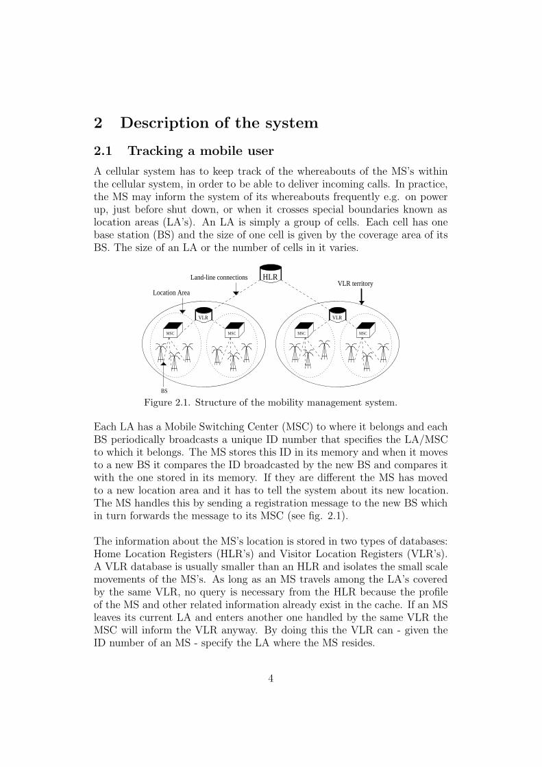
A cellular system has to keep track of the whereabouts of the MS’s withinthe cellular system, in order to be able to deliver incoming calls. In practice,the MS may inform the system of its whereabouts frequently e.g. on powerup, just before shut down, or when it crosses special boundaries known aslocation areas (LA’s). An LA is simply a group of cells. Each cell has onebase station (BS) and the size of one cell is given by the coverage area of itsBS. The size of an LA or the number of cells in it varies.

MSC MSC

VLR

MSC MSC

VLR

HLRLand-line connections

Location AreaVLR territory

BS

Figure 2.1. Structure of the mobility management system.

Each LA has a Mobile Switching Center (MSC) to where it belongs and eachBS periodically broadcasts a unique ID number that specifies the LA/MSCto which it belongs. The MS stores this ID in its memory and when it movesto a new BS it compares the ID broadcasted by the new BS and compares itwith the one stored in its memory. If they are different the MS has movedto a new location area and it has to tell the system about its new location.The MS handles this by sending a registration message to the new BS whichin turn forwards the message to its MSC (see fig. 2.1).

The information about the MS’s location is stored in two types of databases:Home Location Registers (HLR’s) and Visitor Location Registers (VLR’s).A VLR database is usually smaller than an HLR and isolates the small scalemovements of the MS’s. As long as an MS travels among the LA’s coveredby the same VLR, no query is necessary from the HLR because the profileof the MS and other related information already exist in the cache. If an MSleaves its current LA and enters another one handled by the same VLR theMSC will inform the VLR anyway. By doing this the VLR can - given theID number of an MS - specify the LA where the MS resides.

4

2.2 Paging

In current cellular networks - when paging an MS - the final step in the callsetup procedure starts with the MSC sending a page request (PR) to all ofthe BS’s, in the LA where the MS resides, in order to find the MS. However,by monitoring the traffic pattern inside each cell in an LA we can obtaininformation about the system such as probability mass function and move-ment between cells. With this information available it thus seems to be awaste of energy to page all the cells within the LA in order to find the MS.For instance, a sequential search plan that starts with the cells with a higherprobability of discovery should be more efficient.

The PR’s for different MS’s arrives to the MSC in order to be processed in afirst-in first-out (FIFO) matter. Let N be the number of cells, i.e. the num-ber of BS’s, handled by the MSC and let L be the number of paging channelsto each BS. This means that at most L MS’s can be paged simultaneously ineach cell by the MSC. The time epochs at which a PR can be sent to a BSis refered to as a Paging Cycle (PC).

In a first approximation, the paging process is assumed to be perfect in thatif a PR is sent to the BS where the MS resides, and there are available pag-ing channels, it is always paged successfully and discovery takes place withinthat same PC.

Paging with the conventional method goes as follows. First take L PR’s fromthe head of the main queue (if there are L PR’s waiting) in the MSC and sendthese to each the BS’s operating under the MSC. With this method exactlyL MS’s will be discovered per PC and exactly N pagings will be done perMS before discovery. This is a reliable method but it is a waste of systemresources. Why is demonstrated in the following example.

Example 2.1Let say we have a small LA that contains 3 cells and that we have 2 pagingchannels per BS, i.e. N = 3 and L = 2. Say we have 4 PR’s that are waitingat the head of the main queue and denote these A,B,C and D, respectively,and say that MS A and B are in cell 1, C is in cell 2 and D is in cell 3 (seefig 2.2).

5

��

SD Main queueA,B

MSC

D

C

Land-line connections

Incoming PR’s

Figure 2.2. Structure of an MSC with a smart distributor.

Under the conventional algorithm, in the first PC, PR A and B are beingsent to all three cells. In the second PC PR C, and D are being sent to allthe cells.Now let’s have a look at how an “ideal” algorithm would have worked. Insuch a system we would need some kind of distributor that distributes thePR’s among the cells. This distributor will hereafter be refered to as a smartdistributor (SD). The SD buffers the PR’s from the head of the main queueand distributes these among the BS’s. In this case it would buffer all the 4PR’s from the main queue, in the first PC, and send PR A and B to cell 1,PR C to cell 2 and PR D to cell 3.Under the conventional algorithm each MS are paged 3 times (i.e. one timein each cell) as compared to only once in the ideal one and 2 MS’s are beingfound per PC as compared to 4 in the ideal one. Of course, an ideal algorithmwould have to know the exact location of each of the MS’s so the comparisonis therefore not really fair. However, the discussion already points to thepossibility of improving the conventional paging algorithm.

6

3 Algorithms

As the cell sizes shrinks (e.g. microcells and picocells) the probability thatthe MS is moving between the cells during the paging process, gets higher. Agood paging algorithm should take these movement probabilities into consid-eration. This chapter describes some algorithms that can be used for paging.

3.1 Model definition

An MS i placed randomly in one of N cells at time step 1 and then, at eachtime step, it moves between the N cells according to a Markov process.

Let X = {1, 2, ..., N} denote a finite state set and let xk be the state ofthe MS at time step k, i.e. which cell it remains in at time step k. LetA = {1, 2, ..., N} denote a finite action set where action i corresponds to thatcell i is being paged. The decision maker that performs these actions will berefered to as the agent. Further let pk(i) denote the probability of the MSbeing in cell i at time step k. By pk we mean the N -vector with element iequal to pk(i) for 1 ≤ i ≤ N . Let P denote the transition probability matrixi.e. an NxN matrix with element ij equal to

pij = Pr(xk+1 = j|xk = i). (3.1)

Let q(i) denote the probability of being blocked in cell i i.e. the probabilitythat all the paging channels are occupied in cell i when sending a PR to celli. By q we mean the N-vector with element i equal to q(i) for 1 ≤ i ≤ N .Finally, let Θ = {found,missed, blocked} denote a finite observation set andlet θk denote the observation at time step k. The observations are recievedaccording to the known probabilities

rajl = Pr(θk = l|xk = j, ak = a). (3.2)

The observation found corresponds to that the agent is not blocked and theMS is in the cell paged. The observation missed corresponds to that the agentis not blocked but the MS is not in the cell paged. Finally the observationblocked simply means that the agent is blocked in this PC. Consider allvectors to be column vectors.

3.2 The POMDP-algorithm

A partially observable Markov decision process (POMDP) is a generalizationof a Markov decision process (MDP) that allows for incomplete informationregarding the state of the system. The agent must, at each time step, choose

7

an action (i.e. in this case which cell to page), based only on the incompleteinformation at hand. In general, when using POMDP, one of the possibleactions might be to expend resources to gather additional information aboutthe system. Here, we have N actions were each action results in one of threeobservations. Running a POMDP for a specific model gives us the optimalsolution for that model.

The process is initiated with a known probability distribution, p1, among thecells. Let Hk = {p1, a1, θ1, a2, θ2, ..., ak−1, θk−1} denote this initial distributionappended with the history of actions and messages recieved up to time k. Atthe beginning of time step k, Hk contains all the information that the agentcan use to assess the state of the system. If, based on this information, theagent chooses action ak, the following sequence of events is initiated:

1. A real-valued reward g(xk, ak) is recieved for action ak if the state ofthe system is xk.

2. The system transits to a new state xk+1, according to the transitionprobability matrix P .

3. An observation θk is received according to the known probabilities rakxkθk .

4. Time increments by one, Hk+1 = Hk∪{ak, θk}, the agent chooses actionak+1 and the process repeats.

The system evolves, according to the sequence outlined above, through T ≤∞ time epochs, where T is called the horizon. If T <∞ an additional salvagevalue α(i) is received at the beginning of time epoch T + 1 if xT+1 = i. Letα denote the N -vector with components α(i), 1 ≤ i ≤ N . A search policy isan algorithm which specifies the sequence of cells to search. The agent seeksa policy that maximizes the expected net present value of the time stream ofrewards occured during the process:

E{T∑k=1

βk−1g(xk, ak) + βTα(xT+1)}, (3.3)

where 0 ≤ β ≤ 1 is a discount factor. If T = ∞ we require β < 1. When βis large, future rewards play a larger role in the decision process. As β tendsto zero, the agent seeks to maximize the reward for only the next time stepwith no regard for future consequences. Simulations have shown that a β ofabout 0.25! is usually good for our paging models.

Let Ra(θ) denote the NxN diagonal matrix with element (j, j) equal to rajθand let e denote an N -columnvector with a 1 in each component. Define

8

σ(θ|p, a) = p′PRa(θ)e (3.4)

T (θ, p, a) =p′PRa(θ)

σ(θ|p, a). (3.5)

Then σ is the probability of obtaining observation θ given distribution p andaction a and T is, by Baye’s rule, the posterior probability vector pk+1 giventhe prior probability vector pk. Given this, then for T < ∞, the problemof finding a policy that maximizes (3.3) can theoretically be solved (Lovejoy[2]) via the dynamic programming recursion

{V (pT+1) = p′T+1αV (pk) = maxa∈A(p′kg

a + β∑θ∈Θ σ(θ|pk, a)V (T (θ, pk, a))) , k = 1, ..., T,

(3.6)where ga denotes the N-vector with components g(i, a), 1 ≤ i ≤ N . Anypolicy that for each time epoch k maps pk into a maximizing argument in eq.(3.6) will be an optimal policy. V (pk) has the interpretation of the optimalvalue function for the analogous problem with horizon T − k + 1.

3.2.1 Rewards

As mentioned above, the agent seeks a policy that maximizes the stream ofrewards. There are several ways of choosing the reward but not many willgive the optimal policy. We can give the agent a reward every time it findsthe MS, or every time it gets close to the MS. We might also introduce penal-ties by simply put a minus sign in front of the rewards, e.g. give the agent apenalty every time it gets observation missed.

In [3], Eagle gives an account of optimal search in a 2 observation case. Thetwo observations in Eagles paper is found and not found. If the object is inthe searched box i the agent miss it with probability q(i) and gets observationnot found. Eagles reward function is

V (pk, i) = maxa∈Ai

(pk(a)∗(1−q(a))+(1−(1−q(a))∗pk(a))∗V (Ta(pk), a)), (3.7)

where Ta is p updated for an unsuccesful search (i.e. observation not found)in cell a, according to Bayes’s rule (3.5) and Ai ⊆ A. Comparing the firstpart of eq.(3.7) with the first part of eq. (3.6) gives that the rewards ga

should be chosen to

9

ga = (0, 0, ..., 0, 1− q(a), 0, ..., 0, 0)′ (3.8)

i.e. 1−q(a) in the a : th position and 0 elsewhere. If we look at the definitionof ga (eq. (3.6)) this has the interpretation that each time we search the cellwhere the MS resides the agent gets a reward. This reward is equal to theprobability of detecting the MS, given that the MS is in the searched cell.That makes sense because cells with lower q(a), i.e. blocking probability,should be searched more often. This is for the 2 observation case (found andnot found), but ga is independent of the observations. It only depends onthe current state and the current action. This means we should be able touse the same ga in the 3 observation case.

Choosing the reward as above is actually the same as giving the agent a re-ward of 1 each time it finds the MS. The proof of this is available in appendixA.

3.2.2 Solving POMDP’s

When trying to solve eq. (3.6), the fundamental problem is that at each iter-ation of the dynamic programming recursion, Vk must be evaluated for eachpossible pk-vector. This is an infinite set. All feasible numerical methodsinvolve reducing the number of distributions pk considered, for each k, to afinite number.

Tony Cassandra has done a lot of research in POMDP’s and in [4] he de-scribes the POMDP approach to find optimal or near optimal control strate-gies for partially observable stochastic environments, given a complete modelof the environment. On his webpage there are POMPD code available tosolve POMDP’s. These programs are all written in C and the webpage is:http://www.cs.brown.edu/research/ai/pomdp/index.html. Methods that areavailable with these programs includes, among others, the “linear supportalgorithm” (described by Lovejoy in [2]), the “witness algorithm” and “incre-mental pruning” (described in [5]).

How to specify the POMDP-files is described in Appendix B.

3.3 The pq-algorithm

In [6] Rezaiifar and Makowski suggests an algorithm that they call the pq-algorithm. They show that this algorithm is optimal in the 2 observation case(i.e. found and not found) and when the MS doesn’t move between the cellsduring the paging process, and they use this algorithm for the 3 observation

10

case when the MS doesn’t move. The case when the MS doesn’t move willbe refered to as the stationary case.

The pq-algorithm is defined according to a slightly different model. The al-gorithm is then modified to fit to our model.

The MS is placed randomly in one of N cells at time step 1 where it remainsthroghout the paging process. The distribution among the cells is p1(i) fori = 1, ..., N and the observations are found and not found. Let q(i) fori = 1, ..., N be the probability that we get observation not found on a singlePR to cell i, given that the MS is in cell i. This q-vector defined here isidentical to the q-vector defined in chapter 3.1, because the probability thatwe miss the MS, given that we page the cell where the MS resides, is simplythe probability that there are no available paging channels.

The probability of failing to detect the object on the first j − 1 looks in boxi and of succeeding on the j:th, given that the object is in cell i, is

(1− q(i)) ∗ qj−1(i), i = 1, ..., N, j = 1, 2, ... (3.9)

Let r(i, k) denote the number of PR’s out of the k first PR’s that are sent tocell i. Then the pq-algorithm is: choose the (k + 1) : st PR according to

ak+1 = arg maxa∈A

(p1(a) ∗ (1− q(a)) ∗ q(a)r(a,k)), k = 0, 1, 2, 3, ... (3.10)

This is for the 2 observation case. When applying this to the 3 observationcase, Rezaiifaar and Makowski suggest the following in [6]:

• If the agent recieves observation found, then simply stop searching.

• If the agent recieves observation blocked in cell i in the k : th PC, thenincrement r(i, k) by one.

• If the agent recieves observation missed in cell i in the k : th PC, thenset r(i, k) to infinity.

The last point might need some explanation. Setting r(i, k) to infinity hasthe interpretation that the cell has been paged infinite times. Thus it is veryunlikely for the MS to be in that cell. This is for the non-moving case.

Seperate observation not found to the observations blocked and missed ac-tually invalids eq. (3.9) because the probability of being blocked in cell i onone paging attemp now, given that we have been blocked there an arbitrary

11

number of times before is still q(i). This is because we now can observe ifwe get blocked or not in each cell, compared to before when we only knewthe probability that we were blocked. The pq-algorithm still works well, be-cause of the way it spreads out the PR’s among the cells (which leads tomore paging channels available among the cells) and still keeps the numberof PR’s per MS low. However, it’s not optimal anymore when we seperatethe observations.

3.4 The pqup-algorithm

This is an algorithm that was developed during my research and it’s basedon the pq-algorithm. In order to be able to apply the pq-algorithm to themoving case, we have to somehow keep track of the mobile user. One way ofdoing this is to update the p-vector after each time step. We can do this byusing Baye’s rule (eq. (3.5)). However, this equation calculates the p-vectorin the filter case. Filter means that the order of events in one time step isas follows: action→move→observation. For example, if we get observationmissed in cell i, then p(i) = 0 according to eq. (3.5). We can’t use thisp in the pq-algorithm, because the MS moves before next action is taken.The order we really want for this algorithm, in one time step, would be:action→observation→move. This is called the predictor case. This can beobtained by Baye’s rule by simply change the order between P and Ra(θ).Thus,

σp(θ|p, a) = p′Ra(θ)Pe (3.11)

Tp(θ, p, a) =p′Ra(θ)P

σ(θ|p, a), (3.12)

will give us the p-vector that we want.

Now, we can’t set r(i, k) to infinity, when we get observation missed as inthe non-moving case, because then we will never page that cell again. Wemust go back to the original definition of r, i.e. r(i, k) denotes the numberof PR’s out of the k first PR’s that are sent to cell i. The updated p-vectorwill take care of the different observations.

By using eq. (3.11) and eq. (3.12), we can calculate pk+1, given pk, ak andθk. Since we stop searching when we get observation found, we only haveto calculate pk+1 for the observations missed and blocked. The observationmatrix Ra(θ) (defined on page 7) for observation missed and action i is

12

Rak=i(missed) =

1− q(i) · · · 0 0 0 · · · 0...

. . ....

......

. . ....

0 · · · 1− q(i) 0 0 · · · 00 · · · 0 0 0 · · · 00 · · · 0 0 1− q(i) · · · 0...

. . ....

......

. . ....

0 · · · 0 0 0 · · · 1− q(i)

(3.13)

i.e. 0 on the i:th position and 1 − q(i) elsewhere on the diagonal. Insertingthis in eq. (3.11) yields

σp(missed|pk, ak = i) = p′Rak=i(missed)P

1...1

= p′Rak=i(missed)

1...1

= p′

1...101...1

(1− q(i))

= (pk(1) + · · ·+ pk(i− 1) + 0 + pk(i+ 1) + · · ·+ pk(N))(1− q(i))= (1− pk(i))(1− q(i)) (3.14)

Using this σp in eq. (3.12) gives us the posterior p-vector for observationmissed.

p′k+1 = Tp(missed, pk, ak = i) =p′kR

ak=i(missed)P

σp

=(pk(1), . . . , pk(i− 1), 0, pk(i + 1), . . . , pk(N))(1− q(i))P

(1− pk(i))(1− q(i))

=(pk(1), . . . , pk(i− 1), 0, pk(i + 1), . . . , pk(N))P

1− pk(i)(3.15)

For observation blocked the observation matrix is

13

Rak=i(θk = blocked) =

q(i) 0 · · · 0 00 q(i) · · · 0 0...

.... . .

......

0 0 · · · q(i) 00 0 · · · 0 q(i)

(3.16)

Inserting this in eq. (3.11) gives us

σp(blocked|pk, ak = i) = p′Rak=i(blocked)

1...1

= p′

1...1

qk = qk, (3.17)

and finally inserting this in eq. (3.12) gives us the posterior p-vector forobservation blocked

p′k+1 = Tp(blocked, pk, ak = i) =p′kR

ak=i(blocked)P

σp=p′kqkP

qk= p′kP.

(3.18)

3.5 Estimating the q-vector

As mentioned before the probability of being blocked in cell i is the sameas the probability that all the paging channels to cell i are occupied whensending a PR to the cell. The SD-buffer has a size of K and under one PCthe SD distributes the PR’s (maximum K) among the N cells, according tosome algorithm. If more than L PR’s are being sent to a specific cell, inone PC, then some PR’s will be blocked. This means that the true blockingprobabilities, lets call these probabilities qtrue, will depend on the algorithmused, i.e. how it distributes the PR’s among the cells. In turn the algorithmsused here have the q-vector as an in-parameter. The distribution among thecells depends on the choice of this q-vector. This means that the qtrue-vectorwill depend on the choice of q-vector. Of course, we want q to be the sameas qtrue. The question is, how do we choose q to obtain this?

What we can get is an estimate of the qtrue-vector. Let’s call this estimatedvector qtrue and this has the form

qtrue = qtrue + ε, (3.19)

where ε is a random vector representing the estimation error. The qtrue-vector is computed as follows. Fix the p-vector and the q-vector and let the

14

algorithm run for a paging window which consists of W PC’s. Pick W largeenough so that the system reaches steady state. Then, for i = 1, ..., N , letqtrue(i) be the fraction of times that a PR has been denied access to a pagingchannel in cell i within the paging window. It can be shown that this is themaximum likelihood estimation of the qtrue-vector.

The problem is to pick a vector q such that

q(i)− qtrue(i) = 0, i = 1, ..., N. (3.20)

The mapping q → qtrue is virtually impossible to find. There are two manyparameters that affects the mapping, e.g. the number of paging channels,the number of cells, the movement of the MS’s, the size of the SD-buffer,the algorithm used, etc. So when solving eq. (3.20), it calls for some kind ofnumerical approximations.

What we have at our disposal is the input q and the output q − qtrue. Wedon’t have the derivative of the function. This limits the numerical methodswe can use. The method used here is the Robbins-Monro algorithm [7] which,when trying to solve eq. (3.20), yields

qn+1 = qn − bn ∗ (qn − qtrue,n), n = 1, 2, ... (3.21)

and {bn, n = 1, 2, ...} is a sequence of positive numbers. As part of conditionsfor convergence it is required that the gain sequence bn satisfies

∑∞n=1 bn =∞

and∑∞n=1 b

2n < ∞. The usual candidate is bn = n−1. When eq. (3.21) is

defined like this it is required that q(i)−qtrue(i) has a positive derivative. Thisis actually the case, because a higher q(i) means a higher blocking probabilityin cell i and the algorithm used want’s to page cell i less. This leads to thatmore channels will be available in cell i and qtrue will be smaller. Hence,q(i)− q(i)true will be higher and the derivative is positive.

15

4 Numerical results

To be able to compare the different algorithms we introduce two performancemeasures which captures the effiency of the paging. These are

1. F ≡ the expected number of MS’s found per PC.

2. S ≡ the expected number of times that an MS is paged before it isfound.

An efficient algorithm is one that has a higher F and a lower S than theconventional method.

In the simulations the PR’s are generated according to a Poisson processwith rate λ (PR’s/PC). For the conventional method F and S are quitestraightforward to obtain. Each MS is paged exactly N times, since we sendone PR to each of the BS’s for every MS. Therefore

Sconv = N.

Fconv is a bit more difficult to compute. Exactly L MS’s can be paged simul-taneosly with the conventional method. If we assume heavy traffic so thatthere is more than L MS’s to page, then we will discover exactly L MS’sin that PC. Assume that λ is constant long enough for the system to reachsteady state. Then if λ is bigger than L (heavy traffic) the expected numberof MS’s found per PC will be equal to L. However, if λ is smaller than Lthen the expected number of MS’s found per PC will simply be equal to λ,since we can’t discover more MS’s than is coming in. Hence,{

Fconv = λ, λ ≤ LFconv = L, λ ≥ L.

The performances of the different algorithms will be compared with the con-ventional method as the increase in percent in F and the decrease in percentin S.

In all the simulations, the size of the SD buffer (i.e. the maximum numberof PR’s that can be processed per PC) is set to the fixed value K=200. Thisvalue could have been tuned adaptively in response to how many cells beingused, the number of channels per cells, variations in the the input rate λ, etc.This possibility will not be considered further here.

When the agent get the observation blocked, that doesn’t count as a pagingbecause we don’t actually page the MS. With the observation blocked we

16

don’t get any information about the MS location and the PR will remain inthe SD. The higher traffic it is, the higher will the blocking probabilities be.

4.1 The stationary case

Intuitively, in the stationary case (i.e. when the MS doesn’t move), a goodway of paging should be to simply page the cells in decreasing order of theprobabilities p(i), i = 1, ..., N . This is true as long as the traffic isn’t toohigh. The method only minimizes S. With this method, as the traffic getshigher and the main queue starts to grow, the channels to the more attrac-tive cells will be occupied too much and a method that has a higher F ismore attractive. A higher F is exactly what the pq-algorithm gives us. Themethod that pages the cells in decreasing order of p(i) will be referred to asthe p-algorithm.

In the stationary case the performance of the p-algorithm and the pq-algorithmwill be compared.

Simulation I. The stationary caseThis simulation compares the performances as a function of the incomingpaging rate λ. The number of channels L per cell is equal to 9 and the num-ber of cells N is equal to 10. The p1-vector is given in table 4.1.

cell 1 2 3 4 5 6 7 8 9 10p1(i) 0.023 0.12 0.05 0.083 0.21 0.14 0.038 0.095 0.18 0.061

Table 4.1. Listing of the location probabilities among the cells.

In figure 4.1 the increase in discovery rate ((Fseq − Fconv)/Fconv) and thedecrease in signaling load ((Sconv − Sseq)/Sconv) are plotted as a function ofthe incoming paging rate.

17

2 4 6 8 10 12 14 16 18 20−20

0

20

40

60

80

pq

p

PR:s/PC (λ)

Incr

ease

(%)

Increase in discovery rate vs. input rate (λ)

2 4 6 8 10 12 14 16 18 2045

50

55

60

65

pq

p

PR:s/PC (λ)

Dec

reas

e (%

)

Decrease in signaling load vs. input rate (λ)

Figure 4.1. Performance as a function of the incoming paging rate.

The performance of the p-algorithm is independent of the incoming pagingrate. This is because the incoming paging rate change the blocking probabil-ities q and the p-algorithm is independent of these. The p-algorithm alwayshas the minimum possible S. However, when the traffic gets higher and theMQ starts to grow a higher F should be prioritised. When using the p-algorithm the MQ starts to grow when λ ≥ 9. When λ ≤ 9 both algorithmsare able to take care of all the incoming PR’s. For the pq, the MQ starts togrow when λ ≥ 15.5.

A good way to page would be to use the p-algorithm when the traffic isn’theavy, i.e. when the MQ doesn’t grow, because it minimizes S and it takescare of all the incoming PR’s. When the traffic gets higher we should switchto the pq-algorithm, because it’s able to take care of more PR’s per PC.

4.2 The moving case

Running a POMDP for a given model gives us the optimal search policy forthat model. When there is a probability for the MS to move, during the pag-ing process, the best way of paging is not necessarily to page the cell withthe highest pk(i) for k = 1, 2, ..., when the traffic is low as in the stationarycase. This is illustrated in the following example. The example is from [8].

18

Example 4.1Suppose that we have two cells and that q1 = q2 = 0, i.e. we will never beblocked. Also suppose that the transition probability matrix is

P =

(0 1

0.5 0.5

)Now, if p1 = (0.55, 0.45), then an immediate search in cell 1 will lead to dis-covery with probability 0.55 and a search in cell 2 will lead to discovery withprobability 0.45. However, an unsuccessful search in cell 2 will lead to certaindiscovery in the next time step, because it will always move from cell 1 to cell2, whereas an unsuccesful search in cell 1 leads to complete uncertainty asto where it will be in the next time step. Starting to search in cell 2 resultsin an expected cost of 1*0.45+2*0.55=1.55, whereas to start search in cell 1will at best result in an expected cost of 1*0.55+(2*0.5+3*0.5)*0.45=1.675.Hence, starting to search cell 2 is better than to start with cell 1. This isbecause searching cell 2 gives more information about the location.

POMDP solves problems like the one in the example above. There are how-ever, two problems when using POMDP with the paging system. First ofall, the computations becomes very complex and takes a very long time tomake. However, once the computations are made the search policy is givenas a policy graph (described in appendix C) and can easily be applied to thesystem. The second problem - and this is the main problem - is that eq.(3.20) doesn’t seem to have any zeros for the POMDP. The function is bothnegative and positive but it contains discontinuities and it doesn’t seem likethere is any value of q that solves eq. (3.20) for all i. The individual qtrue(i)

′sactually depends on the whole q-vector, so the only case we can plot eq (3.20)is when N = 2. This is done for the pqup in figure 4.2 and for the POMDPin figure 4.3.

19

0

0.5

1

0

0.5

1

−1

−0.5

0

0.5

1

q(1)

q(2)

0

0.5

1

0

0.5

1

−1

−0.5

0

0.5

1

q(1)

q(2)

Figure 4.2. In the left plot, q(1)− qtrue(1) is plotted and in theright plot, q(2)− qtrue(2) is plotted, for the pqup-algorithm.

0

0.5

1

0

0.5

1

−1

−0.5

0

0.5

1

q(1)q(2)

0

0.5

1

0

0.5

1

−1

−0.5

0

0.5

1

q1

q2

Figure 4.3. In the left plot, q(1)− qtrue(1) is plotted and in theright plot, q(2)− qtrue(2) is plotted, for the POMDP.

In figure 4.2 we can find a point where both graphs intersect the zero-plane.The graphs are smooth and the zeros are easy to find. In figure 4.3 we cansee that both graphs contains discontinuities. There is no point where bothgraphs intersect the zeroplane.

4.2.1 Small location areas

In the next two simulations the POMDP is included to check the performance,even though we can’t solve eq. (3.20). For the POMDP the Robbins-Monroehas been running for a longer time (more iterations) and the policy graphthat produced the best performance was saved.

20

Unfortunately, when we’re using POMDP we have to keep the number of cellssmall otherwise the simulations takes to long time to run. In this chapter thenumber of cells in the LA is 4 and the cells are arranged according to figure4.4.

1

2

3

4

Figure 4.4. Structure of the cells in the LA.

The simulations in this chapter compares pqup and POMDP with the conven-tional method and they all have the following transition probability matrixand initial distribution among the cells

P =

0.9 0.05 0.05 0

0.0176 0.9284 0.0206 0.03340.0286 0.0333 0.9047 0.0334

0 0.0344 0.0213 0.9443

p1 = ( 0.12 0.34 0.21 0.33 ).

The MS’s moves roughly one time out of ten between the cells per PC. Thetransition probability matrix is chosen so that pk converge to p1 when we getobservation blocked. To get a P -matrix that makes pk converge like this, theHastings-Metropolis algorithm has been used. This is described in [9].

Simulation II. Light loadAssume a case where L > λ. This means that the conventional method iscapable of discovering all the incoming PR’s. Let the system parameters be{λ = 6 PR’s/PCL = 9

Here, the number of channels per BS is equal to 9 and the conventionalmethod is capable of discovering 9 PR’s per PC. The result is given in table4.2.

21

Fconv 6.0Sconv 4.0

pqup POMDP

Fseq 6.0 6.0Sseq 2.26 2.18Increase in the discovery rate 0 0Decrease in the signaling load 43.6 % 45.5 %

Table 4.2. Results from simulation II.

Even though, q 6= qtrue, for the POMDP, it still has a lower S than the pqupin this case. This is not true for all models, because we can’t solve eq. (3.20)and there doesn’t always exist a good q.

Simulation III. Heavy loadIn this simulation the performances are compared when L < λ. This meansthat the incoming PR’s cannot be taken care of with the conventional method.{λ = 16 PR’s/PCL = 9

Since the system is heavily loaded a higher F should be prioritised before alower S. The result is given in table 4.3.

Fconv 9.0Sconv 4.0

pqup POMDP

Fseq 13.3 11.3Sseq 2.71 2.53Increase in the discovery rate 47.7 % 25.6 %Decrease in the signaling load 32.3 % 36.8 %

Table 4.3. Results from simulation III.

POMDP has a lower F and a lower S than the pqup. When solving POMDPwe only try to minimize S. However, since the MS’s moves among the cells, agood policy graph should spread out the pagings among the cells. This leadsto more available paging channels and a higher F . The F would probably behigher if q = qtrue, for the POMDP.

22

4.2.2 Larger location areas

When the LA’s gets bigger we can’t use POMDP because we would have torun the POMDP for weeks for each model. We would also have to run it formore iterations with the Robbins-Monroe because the more cells we have theharder it is to find a good q. In this chapter the performance of the pqup iscompared with the conventional method in some different situations.

The size of the LA in this chapter is 10 and the cells are arranged as in figure4.5.

1

2

3

4

5

6

7

8

9

10

Figure 4.5. Structure of the cells in the LA.

The model used in the simulations in this chapter is

P =

0.900 0.033 0.000 0.033 0.034 0.000 0.000 0.000 0.000 0.0000.003 0.949 0.019 0.000 0.029 0.000 0.000 0.000 0.000 0.0000.000 0.033 0.900 0.000 0.033 0.034 0.000 0.000 0.000 0.0000.002 0.000 0.000 0.946 0.023 0.000 0.011 0.017 0.000 0.0000.003 0.017 0.011 0.017 0.925 0.017 0.000 0.012 0.000 0.0000.000 0.000 0.017 0.000 0.025 0.919 0.000 0.018 0.021 0.0000.000 0.000 0.000 0.033 0.000 0.000 0.928 0.034 0.000 0.0050.000 0.000 0.000 0.017 0.017 0.017 0.011 0.920 0.016 0.0020.000 0.000 0.000 0.000 0.000 0.033 0.000 0.028 0.936 0.0030.000 0.000 0.000 0.000 0.000 0.000 0.033 0.033 0.034 0.900

p1 = ( 0.011 0.12 0.07 0.15 0.21 0.14 0.051 0.15 0.09 0.008 ).

Once again, the MS’s moves roughly one time out of ten between the cellsper PC and the transition probability matrix is chosen so that pk convergeto p1 when we get observation blocked.

23

Simulation IV. Dependence of the incoming paging rateWe start with the case when L > λ. The system parameters are{λ = 6 PR’s/PCL = 9

The result is given in table 4.4

Fconv 6.0Fseq 6.0Increase in the discovery rate 0

Sconv 10Sseq 4.47Decrease in the signaling load 55.3 %

Table 4.4. Results from simulation IV, light load.

We can see that there is a significant decrease in the signaling load comparedto the conventional method. Let see what happens when the traffic getshigher. The system parameters are given below and the result is given intable 4.5.{λ = 16 PR’s/PCL = 9

Fconv 9.0Fseq 13.8Increase in the discovery rate 52.9 %


Table 4.5. Results from simulation IV, heavy load.

As expected, the two performance measures F and S effects each other. Infigure 4.6 the increase in discovery rate and the decrease in signaling load areplotted as a function of the incoming paging rate, in the case when the MSis moving.

24

2 4 6 8 10 12 14 16 18 20

0

20

40

60

PR:s/PC (λ)

Incr

ease

(%)

Increase in discovery rate vs. input rate (λ)

2 4 6 8 10 12 14 16 18 20

45

50

55

PR:s/PC (λ)

Dec

reas

e (%

)

Decrease in signaling load vs. input rate (λ)

Figure 4.6. Performance as a function of the incoming paging rate

Once again, an increase in F leads to an increase in S and vice versa (com-pare to figure 4.1).

Simulation V. Estimation error in the p-vectorA natural question is how the algorithm works when there is an estimationerror in the model, for example in the p-vector. For a start, let the systemparameters be{λ = 6 PR’s/PCL = 9

Call the estimated p1 for p1. In table 4.6, p1 is listed. The real probabilitydistribution, p1, is repeted for convenience.

p1 0.05 0.16 0.1 0.28 0.15 0.02 0.08 0.12 0.03 0.01p1 0.011 0.12 0.07 0.15 0.21 0.14 0.051 0.15 0.09 0.008

Table 4.6. The estimated and the the real probabilitydistribution vectors used in simulation V.

The result from the simulation is given in table 4.7.

25

Fconv 6.0Fseq 6.0Increase in the discovery rate 0 %


Table 4.7. Results from simulation V,light load and estimated p1.

The fact that the p1-vector may not be estimated precisely didn’t affect theperformance drastically in this case. Let’s see what happens when the trafficgets higher.{λ = 16 PR’s/PCL = 9



Table 4.8. Results from simulation V,heavy load and estimated p1.

Even in this case, the pqup is superior to the conventional method. Thealgorithm may thus be started with a rough estimate of p1.

Simulation VI. Reduced number of paging channelsAn interesting thing to investigate is the performance when fewer channels areallocated for the purpose of paging. Fewer paging channels leaves more radiospectrum available for other transmissions (e.g. voice and data). Therefore,fewer paging channels contributes to the overall improvement of the cellularsystem.

In this simulation the number of paging channels per BS are reduced to 4.We start with an incoming paging rate of 6.

26

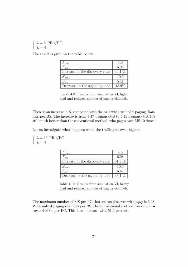
{λ = 6 PR’s/PCL = 4

The result is given in the table below.


Sconv 10.0Sseq 5.41Decrease in the signaling load 45.9%

Table 4.9. Results from simulation VI, lightload and reduced number of paging channels.

There is an increase in S, compared with the case when we had 9 paging chan-nels per BS. The increase is from 4.47 pagings/MS to 5.41 pagings/MS. It’sstill much better than the conventional method, who pages each MS 10 times.

Let us investigate what happens when the traffic gets even higher.{λ = 16 PR’s/PCL = 4


Sconv 10.0Sseq 5.69Decrease in the signaling load 43.1 %

Table 4.10. Results from simulation VI, heavyload and reduced number of paging channels.

The maximum number of MS per PC that we can discover with pqup is 6.08.With only 4 paging channels per BS, the conventional method can only dis-cover 4 MS’s per PC. This is an increase with 51.9 percent.

27

4.3 Conclusions

The simulations showed that both algorithms was superior to the conven-tional method. The pqup proved to be a reliable method and requires littlecomputational power in the MSC’s. The method is robust and works wellboth under low and high traffic, when the number of paging channels is re-duced and when there is an estimation error in the occupancy probabilityvector. Since we couldn’t solve eq. (3.20) for the POMDP , this method isunreliable and doesn’t behave as well as expected. If we somehow could solveeq. (3.20) for the POMDP then this would give us the optimal solution tothe given problem.

28

5 Conclusions

It has been shown that there are several ways of improving the conventionalscheme. The pqup improved the performance significantly. The simulationsshowed that the method

• reduces the signaling load between the MS’s and the MSC’s during thepaging process

• is able to found more MS per PC

• work well both under light and heavy load

• work well with reduced number of paging channels

• is insensitive to the choice of occupancy vector.

The last point has, of course, practical significance since obtaining an occu-pancy probability vector that captures the occupancy probabilities of all theMS’s is a practical impossibility.

The POMDP-algorithm didn’t work as well as expected. Even though itworked better than the pqup in some cases, we can’t use the POMDP as apaging scheme, as long as we can’t solve eq. (3.20). If we could, then thisalgorithm would have been optimal for the given model.

5.1 Future work

The research about using POMDP as a paging scheme is going to be contin-ued. The main research is going to be about how we can specify the modelin a way that we can solve eq. (3.20). Maybe we can use different rewardsor different observations?

29

A Rewards

Here it will be shown that giving the agent a reward that equals the prob-ability of detection, given that the MS resides in the searched cell a, (i.e.1 − q(a)), is equal to give the agent a reward of 1, each time he finds theobject.

To begin with, we write the reward function g as a function of action, stateand observation, i.e. g(ak, xk, θk). This is the reward the agent recieveswhen he searches cell ak, the object is in cell xk and the agent recieves theobservation θk at time step k. We start with the 2 observation case so theobservations are either found or not found. If the agent recieves reward Ri

each time he finds the object in cell i and the penalty for paging cell i is Ci,then the reward functions will be

g(xk = i, ak = i, θk = notfound) = −Cig(xk = i, ak = i, θk = found) = Ri − Cig(xk = i, ak = j, θk = notfound) = −Ci, i 6= jg(xk = i, ak = j, θk = found) = Ri − Ci, i 6= j.

(A.1)

Of course, the last reward will never be obtained, because if the agent pagethe wrong cell it will never find the object, but it’s written here anyway forthe sake of concretness. Now we can write the reward function as a functionof action and state (i.e. as defined on page 7)

g(xk = i, ak = i)

= g(xk = i, ak = i, θk = notfound) ∗ Pr(θk = notfound|xk = i, ak = i)

+g(xk = i, ak = i, θk = found) ∗ Pr(θk = found|xk = i, ak = i)

= −Ci ∗ qi + (Ri − Ci) ∗ (1− qi) = Ri ∗ (1− qi)− Ci

and

g(xk = i, ak = j)

= g(xk = i, ak = j, θk = notfound) ∗ Pr(θk = notfound|xk = i, ak = j)

+g(xk = i, ak = j, θk = found) ∗ Pr(θk = found|xk = i, ak = j)

= −Ci ∗ 1 + (Ri − Ci) ∗ 0 = −Ci.

This gives us ga as defined in eq. (3.6).

ga = (−Ca,−Ca, ...,−Ca, Ra ∗ (1− qa)− Ca,−Ca, ..., Ca, Ca)′. (A.2)

30

Putting this in eq. (3.6) yields,

V (pk) = maxa∈A

(p′kga + β

∑θ∈Θ

σ(θ|pk, a)V (T (θ, pk, a)))

= maxa∈A

(p′k ∗ (−Ca, ...,−Ca, Ra ∗ (1− q(a))− Ca, ..., Ca)′

+β∑θ∈Θ


= maxa∈A

(pk(a) ∗Ra ∗ (1− q(a))− Ca

+β∑θ∈Θ


Comparing this result with Eagle’s (eq. (3.7)) gives that the reward Ri shouldbe chosen to 1 for i = 1, ..., N and the penalty Ci should be choosen to 0 fori = 1, ..., N . However, since Ci is just a constant and it is in a maximisationexpression, we can choose Ci to any constant we want (as long as it the samefor all i). Eagle just chosed it to be 0. As a matter of fact, we can actuallychoose the reward to be any constant ≥ 0 as long as it’s the same for all cells.This is a bit harder to see and it won’t be discussed further here.

31

B The POMDP-file

B.1 POMDP-file specification

POMDP solve version 4.0 written by A. R. Cassandra.

This describes the POMDP file format.

There are some semantics to the format and these are discussed here. Allfloating point number must be specified with at least one digit before andone digit after the decimal point.

Comments: Everything from a ’#’ symbol to the end-of-line is treated as acomment. They can appear anywhere in the file.

The following 5 lines must appear at the beginning of the file. They mayappear in any order as long as they preceed all specifications of transitionprobabilities, observation probabilities and rewards.

discount: %fvalues: [ reward, cost ]states: [ %d, <list of states> ]actions: [ %d, <list of actions> ]observations: [ %d, <list of observations> ]

The definition of states, actions and/or observations can be either a numberindicating how many there are or it can be a list of strings, one for each entry.These mnemonics cannot begin with a digit. For instance, both:

actions: 4actions: north south east west

will result in 4 actions being defined. The only difference is that, in the latter,the actions can then be referenced in this file by the mnemonic name. Evenwhen mnemonic names are used, later references can use a number as well,though it must correspond to the positional numbering starting with 0. Thenumbers are assigned consecutively from left to right in the listing startingwith zero. The mnemonics are discarded once the whole file has been read in.

When listing states, actions or observations one or more whitespace char-acters are the delimiters (space, tab or newline). When a number is giveninstead of an enumeration, the individual elements will be referred to by con-

32

secutive integers starting at 0.

After the preamble, there is the optional specification of the starting state.For the current POMDP-solve code, this is completely ignored. It allows itto parse it to be compatible with newer versions of the specification. Thereare a number of different formats for the starting state, but these won’t bediscussed here. You won’t need them for this program, and if you are runningthem on a file that has them, then you’ll know what they look like.

After the initial five lines and optional starting state, the specifications oftransition probabilities, observation probabilities and rewards appear. Thesespecifications may appear in any order. Any probabilities or rewards notspecified in the file are assumed to be zero.

You may also specify a particular probability or reward more than once. Thedefinition that appears last in the file is the one that will take affect. This isconvenient for specifying exceptions to a more general specification.

To specify an individual transition probability:

T: <action> : <start-state> : <end-state> %f

Anywhere an action, state or observation can appear, you can also put thewildcard character ’∗’ which means that this is true for all possible entriesthat could appear here. For example:

T: 5 : ∗ : 0 1.0

is interpreted as action 5 always moving the system state to state 0, no mat-ter what the starting state was (i.e., for all possible starting states.)

To specify a single row of a particular actions transition matrix:

T: <action> : <start-state>%f %f ... %f

Where there is an entry for each possible next state. This allows defining thespecific transition probabilities for a particular starting state only. Instead ofa list of probabilities the mnemonic word ’uniform’ may appear. In this case,each transition for each next state will be assigned the probability 1/#states.Again, an asterick in either the action or start-state position will indicate allpossible entries that could appear in that position.

33

To specify an entire transition matrix for a particular action:

T: <action>%f %f ... %f%f %f ... %f. . .%f %f ... %f

Where each row corresponds to one of the start states and each column spec-ifies one of the ending states. Each entry must be separated from the nextwith one or more white-space characters. The state numbers goes from leftto right for the ending states and top to bottom for the starting states. Thenew-lines are just for formatting convenience and do not affect final matrixresults. The only restriction is there must be NxN values specified where Nis the number of states.

In addition, there are a few mnemonic conventions that can be used in placeof the explicit matrix:

identityuniform

Note that uniform means that each row of the transition matrix will be setto a uniform distribution. The identity mnemonic will result in a transitionmatrix that leaves the underlying state unchanged for all possible startingstates (i.e., the identity matrix).

The observational probabilities are specified in a manner similiar to the tran-sition probabilities. To specify individual observation probabilities:

O : <action> : <end-state> : <observation> %f

The asterick wildcard is allowed in any of the positions.

34

To specify a row of a particular actions observation probability matrix:

O : <action> : <end-state>%f %f ... %f

This specifies a probability of observing each possible observation for a par-ticular action and ending state. The mnemonic short-cut ’uniform’ may alsoappear in this place.

To specify an entire observation probability matrix for an action:

O: <action>%f %f ... %f%f %f ... %f. . .%f %f ... %f

The format is similiar to the transition matrices except the number of entriesmust be NxO where N is the number of states and O is the number of ob-servations. Again, the ’uniform’ mnemonic can be substituted for an entirematrix. In this case it will assign each entry of each row the probability1/#observations.

To specify individual rewards:

R: <action> : <start-state> : <end-state> : <observation> %f

For any of the entries, an asterick for either <state>, <action>, <observation>indicates a wildcard that will be expanded to all existing entities.

There are two other forms to specify rewards:

R: <action> : <start-state> : <end-state>%f %f ... %f

This specifies a particular row of a reward matrix for a particular action andstart state. The last reward specification form is

35

R: <action> : <start-state>%f %f ... %f%f %f ... %f. . .%f %f ... %f

which lets you specify an entire reward matrix for a particular action andstart-state combination.

B.2 A POMDP-file example

Here is a POMDP-file example running on the paging system. There are 3observations and the reward 1 is obtained when the agent receives observa-tion found. The number of states is 3, the transition probability matrix is

P =

0.9 0.05 0.050.05 0.9 0.050.05 0.05 0.9

and the blocking probabilities are

q = ( 0.25 0.4 0.1 ).

One way to specify the POMDP-file for this model is:

discount: 0.25values: rewardstates: 3actions: 3observations: found missed blocked

T: *0.9 0.05 0.050.05 0.9 0.050.05 0.05 0.9

O: 00.75 0 0.250 0.75 0.250 0.75 0.25

36

O: 10 0.6 0.40.6 0 0.40 0.6 0.4

O: 20 0.9 0.10 0.9 0.10.9 0 0.1

R: * : * : *1 0 0

37

C The result-files after a POMDP simulation

After running a POMDP simulation, the POMDP program will give you thesolution in two files. How to use these files are described here.

C.1 The alpha-file

This file lists the alpha vectors after a POMDP simulation. The vectors fullyspecifies the solution after running a simulation. Each vector has an actionassociated with it and, at time step k, we should pick the vector accordingto eq. (C.1), (compare to eq. (3.6)).

arg maxj

(pkαj), j = 1, ..., J, (C.1)

where J is the number of vectors. After picking an alpha vector we choosethe action associated with it. This is the action for time step k. The formatof the alpha-file is simply:

<action> <list of vector components>

<action> <list of vector components>

etc...

The number of alpha vectors is equal to the number of states in the POMDP.

C.2 The pg-file

Another (and more convenient) way to specify the solution after a POMDPsimulation is to use a policy graph. With a policy graph we don’t have tocalculate pk at each time step. We only have to know the initial locationdistribution probability vector, p1. Each line in the pg-file represents onenode of the policy graph and its contents are:

N A Z1 Z2 Z3 ...

Here ’N’ is a node ID giving the node a unique name. ’A’ is an integer andspecifies the action associated with this node. These are followed by a list ofnode ID’s, one for each observation. Thus the list will have a length equal tothe number of observations in the POMDP. This list specifies the transitionsin the policy graph. If the observation recieved is n, then the n : th element

38

in the list will specify the next node in the policy graph. The start node inthe policy graph is specified (from the alpha-file) by eq. (C.2).

arg maxj

(p1αj), j = 1, ..., J. (C.2)

39

D Abbreviations

This abbreviations are all defined earlier in the paper. They are written herefor convinience.

BS: Base Station, each cell has one base station.

HLR: Home Location Register, contains information about the whereaboutsof the mobile stations but is usually bigger than a visitor location reg-ister and it caches portions of information to these.

LA: Location Area, a geographic area covered by a group of cells.

MS: Mobile Station, a mobile communication device, e.g. a mobile phone.

MSC: Mobile Switching Center, manages the base stations within a locationarea.

PC: Paging Cycle, the time epoch at which a page request can be sent to abase station.

PR: Page Request, a request to page a mobile station in a specific cell.

SD: Smart Distributor, distributes the page requests among the cells.

VLR: Visitor Location Register, contains information about the where-abouts of the mobile stations. It isolates the small-scale movements.

40

References

[1] T.S. Rappaport, Wireless Communications. Prentice Hall, 1996.

[2] W.S. Lovejoy, “A survey of alghorithmic methods for partially observedMarkov decision processes”. Annals of Operations Research 28, pp. 47-65, 1991.

[3] J.N. Eagle, “The optimal search for a moving target when the searchpath is constrained”. Operations Research, vol. 32, pp. 1107-1115, 1984.

[4] A.R. Cassandra, L.P. Kaelbling, M.L. Littman, “Act-ing optimally in partially observable stochastic domains”.http://www.cs.duke.edu/ mlittman/topics/pomdp-page.html, link:“POMDP’s as a model of planning”.

[5] A.R. Cassandra, M.L. Littman, N.L. Zang, “Incremental Prun-ing, a simple, fast, exact method for partially observable Markovdecision processes”. http://www.cs.duke.edu/ mlittman/topics/pomdp-page.html, link: “POMDP algorithms”.

[6] R. Rezaiifar, A.M. Makowski, “From optimal search theory to sequen-tial paging in cellullar networks”. IEEE Journal on Selected Areas inCommunications, vol. 15, no. 17, pp. 1253-1264, september 1997.

[7] M.T. Wasan, Stochastic Approximation. New York: Cambridge Uni-versity, 1969.

[8] S.M. Ross, Introduction to Stochastic Dynamic Programming. Aca-demic press, 1983.

[9] S.M. Ross, Simulation. San Diego: Academic Press, 1997, 2:nd ed.

41

sequential paging for moving mobile users · issn 0280{5316 isrn lutfd2/tfrt--5636--se sequential...

Documents