Smooth Calibration, Leaky Forecasts, Finite Recall and Nash Dynamics

2 November 2017, 11:15-12:30, bld. 72, room 465

Sergiu Hart (HUJI)

Abstract: We propose to smooth out the calibration score, which measures

how good a forecaster, is, by combining nearby forecasts. While regular

calibration can be guaranteed only by randomized forecasting procedures,

we show that smooth calibration can be guaranteed by deterministic

procedures. As a consequence, it does not matter if the forecasts are leaked,

i.e., made known in advance: smooth calibration can nevertheless be guaranteed

(while regular calibration cannot). Moreover, our procedure has finite recall,

is stationary, and all fore-casts lie on a finite grid. To construct it, we deal also

with the related setups of online linear regression and weak calibration.

Finally, we show that smooth calibration yields uncoupled finite-memory

dynamics in n-person games—“smooth calibrated learning”—in which the

players play approximate Nash equilibria in almost all periods.

Smooth Calibration, Leaky Forecasts, Finite

Recall, and Nash Dynamics∗

Dean P. Foster† Sergiu Hart‡

March 30, 2017

Abstract

We propose to smooth out the calibration score, which measures

how good a forecaster is, by combining nearby forecasts. While reg-

ular calibration can be guaranteed only by randomized forecasting

procedures, we show that smooth calibration can be guaranteed by

deterministic procedures. As a consequence, it does not matter if

the forecasts are leaked, i.e., made known in advance: smooth calibra-

tion can nevertheless be guaranteed (while regular calibration cannot).

Moreover, our procedure has finite recall, is stationary, and all fore-

casts lie on a finite grid. To construct it, we deal also with the related

setups of online linear regression and weak calibration. Finally, we

show that smooth calibration yields uncoupled finite-memory dynam-

ics in n-person games—“smooth calibrated learning”—in which the

players play approximate Nash equilibria in almost all periods.

∗Previous versions: July 2012, February 2015. Research of the second author waspartially supported by a European Research Council (ERC) Advanced Investigator grant.The authors thank Yakov Babichenko for useful comments and suggestions.

†Amazon Inc, New York City, and University of Pennsylvania, Philadelphia. e-mail :dean@foster.net web page: http://deanfoster.net/

‡Institute of Mathematics, Department of Economics, and Center for the Study ofRationality, The Hebrew University of Jerusalem. e-mail : hart@huji.ac.il web page:http://www.ma.huji.ac.il/hart

1

Contents

1 Introduction 2

1.1 Literature . . . . . . . . . . . . . . . . . . . . . . . . . . . . . 4

2 Model and Result 5

2.1 The Calibration Game . . . . . . . . . . . . . . . . . . . . . . 5

2.2 Smooth Calibration . . . . . . . . . . . . . . . . . . . . . . . . 6

2.3 Leaky Forecasts . . . . . . . . . . . . . . . . . . . . . . . . . . 8

2.4 Result . . . . . . . . . . . . . . . . . . . . . . . . . . . . . . . 9

3 Online Linear Regression 10

3.1 Forward Algorithm . . . . . . . . . . . . . . . . . . . . . . . . 11

3.2 Discounted Forward Algorithm . . . . . . . . . . . . . . . . . 12

3.3 Windowed Discounted Forward Algorithm . . . . . . . . . . . 16

4 Weak Calibration 20

5 Smooth Calibration 25

6 Nash Equilibrium Dynamics 30

References 39

A Appendix 41

1 Introduction

How good is a forecaster? Assume for concreteness that every day the fore-

caster issues a forecast of the type “the chance of rain tomorrow is 30%.” A

simple test one may conduct is to calculate the proportion of rainy days out

of those days that the forecast was 30%, and compare it to 30%; and do the

same for all other forecasts. A forecaster is said to be calibrated if, in the

long run, the differences between the actual proportions of rainy days and

2

the forecasts are small—no matter what the weather really was (see Dawid

1982).

What if rain is replaced by an event that is under the control of another

agent? If the forecasts are made public before the agent decides on his

action—we refer to this setup as “leaky forecasts”—then calibration cannot

be guaranteed; for example, the agent can make the event happen if and

only if the forecast is less than 50%, and so the forecasting error (that is, the

“calibration score”) is always at least 50%. However, if in each period the

forecast and the agent’s decision are made “simultaneously”—which means

that neither one knows the other’s decision before making his own—then

calibration can be guaranteed; see Foster and Vohra (1998). The procedure

that yields calibration no matter what the agent’s decisions are requires the

use of randomizations (e.g., with probability 1/2 the forecaster announces

30%, and with probability 1/2 he announces 60%). Indeed, as the discussion

at the beginning of this paragraph suggests, one cannot have a deterministic

procedure that is calibrated (see Oakes 1985).

Now the standard calibration score is very sensitive: the days when the

forecast was, say, 30% are considered separately from the days when the

forecast was 29.99% (formally, the calibration score is a highly discontinuous

function of the data, i.e., the forecasts and the actions). This suggests that

one first combine all days when the forecast was close to 30%, and only then

compare the 30% with the appropriate average proportion of rainy days.

Formally, it amounts to a so-called “smoothing” operation.

Perhaps surprisingly, once we consider smooth calibration, there is no

longer a need for randomization when making the forecasts: we will show

that there exist deterministic procedures that guarantee smooth calibration,

no matter what the agent does. In particular, it follows that it does not

matter if the forecasts are made known to the agent before his decision, and

so smooth calibration can be guaranteed also when forecasts may be leaked.1

Moreover, the forecasting procedure that we construct and which guaran-

1Even if the forecast is not leaked, the agent can simulate the deterministic calibrationprocedure and generate the forecast by himself. Our procedure indeed takes this intoaccount.

3

tees smooth calibration has finite recall (i.e., only the forecasts and actions

of the last R periods are taken into account, for some fixed finite R), and

is stationary (i.e., independent of “calendar time”: the forecast is the same

any time that the “window” of the past R periods is the same).2 Finally, we

can have all the forecasts lie on some finite fixed grid.

The construction starts with the “online linear regression” problem, in-

troduced by Foster (1991), where one wants to generate every period a good

linear estimator based only on the data up to that point. We provide a

finite-recall stationary algorithm for this problem; see Section 3. We then

use this algorithm, together with a fixed-point argument, to obtain “weak

calibration,” a concept introduced by Kakade and Foster (2004) and Foster

and Kakade (2006); see Section 4. Section 5 shows that weak and smooth

calibration are essentially equivalent, which yields the existence of smoothly

calibrated procedures. Finally, these procedures are used to obtain dynam-

ics (“smoothly calibrated learning”) that are uncoupled, have finite memory,

and are close to Nash equilibria most of the time.

1.1 Literature

The calibration problem has been extensively studied, starting with Dawid

(1982), Oakes (1985), and Foster and Vohra (1998); see Olszewski (2015)

for a comprehensive survey of the literature. Kakade and Foster (2004) and

Foster and Kakade (2006) introduced the notion of weak calibration, which

shares many properties with smooth calibration. In particular, both can be

guaranteed by deterministic procedures, and both are of the “general fixed

point” variety: they can find fixed points of arbitrary continuous functions

(see for instance the last paragraph in Section 2.3).3 However, while weak

calibration may be at times technically more convenient to work with, smooth

calibration is the more natural concept, easy to interpret and understand; it

2One way to obtain this is by restarting the procedure once in a while; see, e.g., Lehrerand Solan (2009).

3They are thus more “powerful” than the standard calibration procedures, such as thosebased on Blackwell’s approachability, which find linear fixed points, such as eigenvectorsand invariant probabilities.

4

is, after all, just a standard smoothing of regular calibration.

The online regression problem—see Section 3 for details—was introduced

by Foster (1991); for further improvements, see J. Foster (1999), Vovk (2001),

Azoury and Warmuth (2001), and the book of Cesa-Bianchi and Lugosi

(2006).

2 Model and Result

In this section we present the calibration game in its standard and “leaky”

versions, introduce the notion of smooth calibration, and state our main

results.

2.1 The Calibration Game

Let4 C ⊆ Rm be a compact convex set, and let A ⊆ C (for example, C

could be the set of probability distributions ∆(A) over a finite set A, which

is identified with the set of unit vectors in C). The calibration game has two

players: the “action” player—the “A-player” for short—and the “conjecture”

(or “calibrating”) player—the “C-player” for short. At each time period

t = 1, 2, ..., the C-player chooses ct ∈ C and the A-player chooses at ∈ A.

There is full monitoring and perfect recall: at time t both players know the

realized history ht−1 = (c1, a1, ..., ct−1, at−1) ∈ (C × A)t−1.

In the standard calibration game, ct and at are chosen simultaneously

(perhaps in a mixed, i.e., randomized, way). In the leaky calibration game,

at is chosen after ct has been chosen and revealed; thus, ct is a function of

ht−1, whereas at is a function of ht−1 and ct. Formally, a pure strategy of the

C-player is σ : ∪t≥1(C × A)t−1 → C, and a pure strategy of the A-player is

τ : ∪t≥1(C×A)t−1 → A in the standard game, and τ : ∪t≥1(C×A)t−1×C → A

in the leaky game. A pure strategy of the C-player will also be referred to

as deterministic.

The calibration score—which the C-player wants to minimize—is defined

4R

m denotes the m-dimensional Euclidean space, with the usual ℓ2-norm || · ||.

5

at time T = 1, 2, ... as

KT =1

T

T∑

t=1

||at − ct||,

where

at :=

∑Ts=1 1cs=ct

as∑T

s=1 1cs=ct

;

here 1x=y is the indicator that x = y (i.e., 1x=y = 1 when x = y and 1x=y = 0

otherwise). Thus KT is a function of the whole history hT ∈ (C × A)T ; it is

the mean distance between the forecast c and the average a of the actions a

chosen in those periods where the forecast was c.

2.2 Smooth Calibration

We introduce the notion of “smooth calibration.” A smoothing function is a

function Λ : C × C → [0, 1] with Λ(c, c) = 1 for every c. Its interpretation is

that Λ(c′, c) gives the weight that we assign to c′ when we are at c; we will

use Λ(c′, c) instead of the indicator 1c′=c to “smooth” out the forecasts and

the average actions. Specifically, put

aΛt :=

∑Ts=1 Λ(cs, ct) as

∑Ts=1 Λ(cs, ct)

and cΛt :=

∑Ts=1 Λ(cs, ct) cs

∑Ts=1 Λ(cs, ct)

.

The Λ-smoothed calibration score at time T is then defined as

KΛT =

1

T

T∑

t=1

||aΛt − cΛ

t ||. (1)

A standard (and useful) assumption is a Lipschitz condition: there exists

L < ∞ such that |Λ(c′, c) − Λ(c′′, c)| ≤ L||c′ − c′′|| for all c, c′, c′′ ∈ C. Thus,

the functions Λ(·, c) are uniformly Lipschitz: L(Λ(·, c)) ≤ L for every c ∈ C,

where L(f) := sup‖f(x) − f(y)‖ / ‖x − y‖ : x, y ∈ X, x 6= y denotes the

Lipschitz constant of the function f (if f is not a Lipschitz function then

L(f) = +∞; when L(f) ≤ L we say that f is L-Lipschitz ).

Two classical examples of Lipschitz smoothing functions are: (i) Λ(c′, c) =

6

[1 − ||c′ − c||/δ]+ for5 δ > 0: only points within distance δ of c are con-

sidered, and their weight is proportional to the distance from c; and (ii)

Λ(c′, c) = exp(−||c′− c||2/(2σ2)): the weight is given by a Gaussian (normal)

perturbation.

Remarks. (a) The original calibration score KT is obtained when Λ is the

indicator function: Λ(c′, c) = 1c′=c for all c, c′ ∈ C.

(b) The normalization Λ(c, c) = 1 pins down the Lipschitz constant (oth-

erwise one could replace Λ with αΛ for small α > 0, and so lower the Lipschitz

constant without affecting the score).

(c) Smoothing both at and ct and then taking the difference is the same

as smoothing the difference: aΛt − cΛ

t = (at − ct)Λ. Moreover, smoothing at is

the same as smoothing at, i.e., aΛt = aΛ

t .

(d) An alternative score smoothes only the average action at, but not the

forecast ct:

KΛT =

1

T

T∑

t=1

||aΛt − ct||.

If the smoothing function puts positive weight only in small neighborhoods,

i.e., there is δ > 0 such that Λ(c′, c) > 0 only when ||c′ − c|| ≤ δ, then the

difference between KΛT and KΛ

T is at most δ (because in this case ||cΛt −ct|| ≤ δ

for every t). More generally, |KΛT − KΛ

T | ≤ δ when (1/T )∑T

t=1 ||cΛt − ct|| ≤

δ for any collection of points c1, ..., cT ∈ C, which is indeed the case, for

instance, for the Gaussian smoothing with small enough σ2. The reason that

we prefer to use KΛ rather than KΛ is that KΛ vanishes when there is perfect

calibration (i.e., at = ct for all t), whereas KΛ is positive; clean statements

such as KΛT ≤ ε become KΛ

T ≤ ε + δ.

Finally, given ε > 0 and L < ∞, we will say that a strategy of the C-

player—which is also called a “procedure”—is (ε, L)-smoothly calibrated if

there is T0 ≡ T0(ε, L) such that

KΛT =

1

T

T∑

t=1

∥

∥aΛt − cΛ

t

∥

∥ ≤ ε (2)

5Where [z]+ = maxz, 0. These Λ functions are sometimes called “tent functions.”

7

holds almost surely, for every strategy of the A-player, every T > T0, and

every smoothing function Λ : C × C → [0, 1] that is L-Lipschitz in the

first coordinate. Unlike standard calibration, which can be guaranteed only

with high probability, smooth calibration may be obtained by deterministic

procedures—as will be shown below—in which case we may well require (2)

to always hold (rather than just almost surely).

2.3 Leaky Forecasts

We willl say that a procedure (i.e., a strategy of the C-player) is (smoothly)

leaky-calibrated if it is (smoothly) calibrated also in the leaky setup, that

is, against an A-player who may choose his action at at time t depending

on the forecast ct made by the C-player at time t (i.e., the A-player moves

after the C-player). While, as we saw in the Introduction, there are no leaky-

calibrated procedures, we will show that there are smoothly leaky-calibrated

procedures.

Deterministic procedures (i.e., pure strategies of the C-player) are clearly

leaky: the A-player can use the procedure at each period t to compute ct as

a function of the history ht−1, and only then determine his action at. Thus,

in particular, there cannot be deterministic calibrated procedures (because

there no leaky such procedures).

In the case of smooth calibration, the procedure that we construct is

deterministic, and thus smoothly leaky-calibrated. However, there are also

randomized smooothly leaky-calibrated procedures. One example is the sim-

ple calibrated procedure of Foster (1999) in the one-dimensional case (where

A = “rain”, “no rain” and C = [0, 1]): the forecast there is “almost deter-

ministic”, and so can be shown to be smoothly leaky-calibrated. For another

example, see footnote 21 in Section 4 below.

A particular instance of the leaky setup is one where the A-player uses a

fixed reaction function g : C → A that is a continuous mapping of forecasts

to actions; thus, at = g(ct) (independently of time t and history ht−1). In

this case, smooth leaky-calibration implies that most of the forecasts that are

used must be approximate fixed points of g; indeed, in every period in which

8

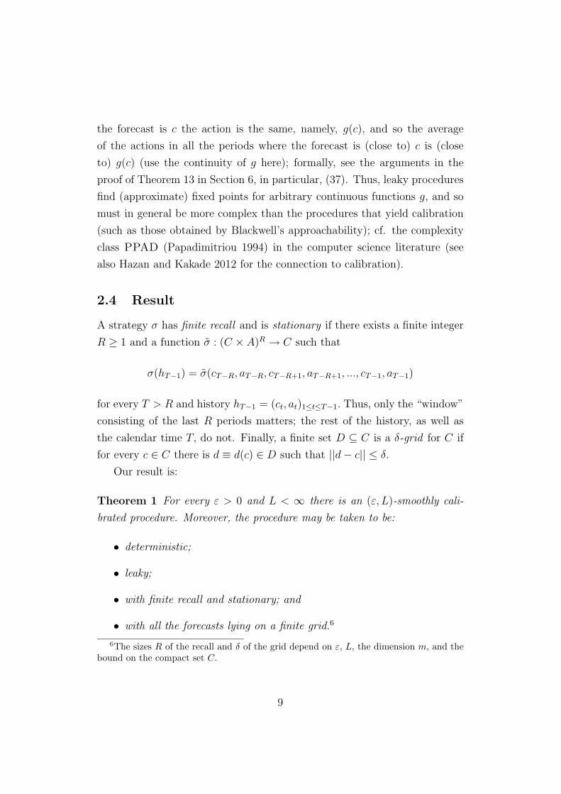
the forecast is c the action is the same, namely, g(c), and so the average

of the actions in all the periods where the forecast is (close to) c is (close

to) g(c) (use the continuity of g here); formally, see the arguments in the

proof of Theorem 13 in Section 6, in particular, (37). Thus, leaky procedures

find (approximate) fixed points for arbitrary continuous functions g, and so

must in general be more complex than the procedures that yield calibration

(such as those obtained by Blackwell’s approachability); cf. the complexity

class PPAD (Papadimitriou 1994) in the computer science literature (see

also Hazan and Kakade 2012 for the connection to calibration).

2.4 Result

A strategy σ has finite recall and is stationary if there exists a finite integer

R ≥ 1 and a function σ : (C × A)R → C such that

σ(hT−1) = σ(cT−R, aT−R, cT−R+1, aT−R+1, ..., cT−1, aT−1)

for every T > R and history hT−1 = (ct, at)1≤t≤T−1. Thus, only the “window”

consisting of the last R periods matters; the rest of the history, as well as

the calendar time T, do not. Finally, a finite set D ⊆ C is a δ-grid for C if

for every c ∈ C there is d ≡ d(c) ∈ D such that ||d − c|| ≤ δ.

Our result is:

Theorem 1 For every ε > 0 and L < ∞ there is an (ε, L)-smoothly cali-

brated procedure. Moreover, the procedure may be taken to be:

• deterministic;

• leaky;

• with finite recall and stationary; and

• with all the forecasts lying on a finite grid.6

6The sizes R of the recall and δ of the grid depend on ε, L, the dimension m, and thebound on the compact set C.

9

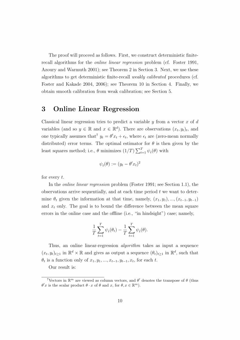
The proof will proceed as follows. First, we construct deterministic finite-

recall algorithms for the online linear regression problem (cf. Foster 1991,

Azoury and Warmuth 2001); see Theorem 2 in Section 3. Next, we use these

algorithms to get deterministic finite-recall weakly calibrated procedures (cf.

Foster and Kakade 2004, 2006); see Theorem 10 in Section 4. Finally, we

obtain smooth calibration from weak calibration; see Section 5.

3 Online Linear Regression

Classical linear regression tries to predict a variable y from a vector x of d

variables (and so y ∈ R and x ∈ Rd). There are observations (xt, yt)t, and

one typically assumes that7 yt = θ′xt + ǫt, where ǫt are (zero-mean normally

distributed) error terms. The optimal estimator for θ is then given by the

least squares method; i.e., θ minimizes (1/T )∑T

t=1 ψt(θ) with

ψt(θ) := (yt − θ′xt)2

for every t.

In the online linear regression problem (Foster 1991; see Section 1.1), the

observations arrive sequentially, and at each time period t we want to deter-

mine θt given the information at that time, namely, (x1, y1), ..., (xt−1, yt−1)

and xt only. The goal is to bound the difference between the mean square

errors in the online case and the offline (i.e., “in hindsight”) case; namely,

1

T

T∑

t=1

ψt(θt) −1

T

T∑

t=1

ψt(θ).

Thus, an online linear-regression algorithm takes as input a sequence

(xt, yt)t≥1 in Rd × R and gives as output a sequence (θt)t≥1 in R

d, such that

θt is a function only of x1, y1, ..., xt−1, yt−1, xt, for each t.

Our result is:

7Vectors in Rm are viewed as column vectors, and θ′ denotes the transpose of θ (thus

θ′x is the scalar product θ · x of θ and x, for θ, x ∈ Rm).

10

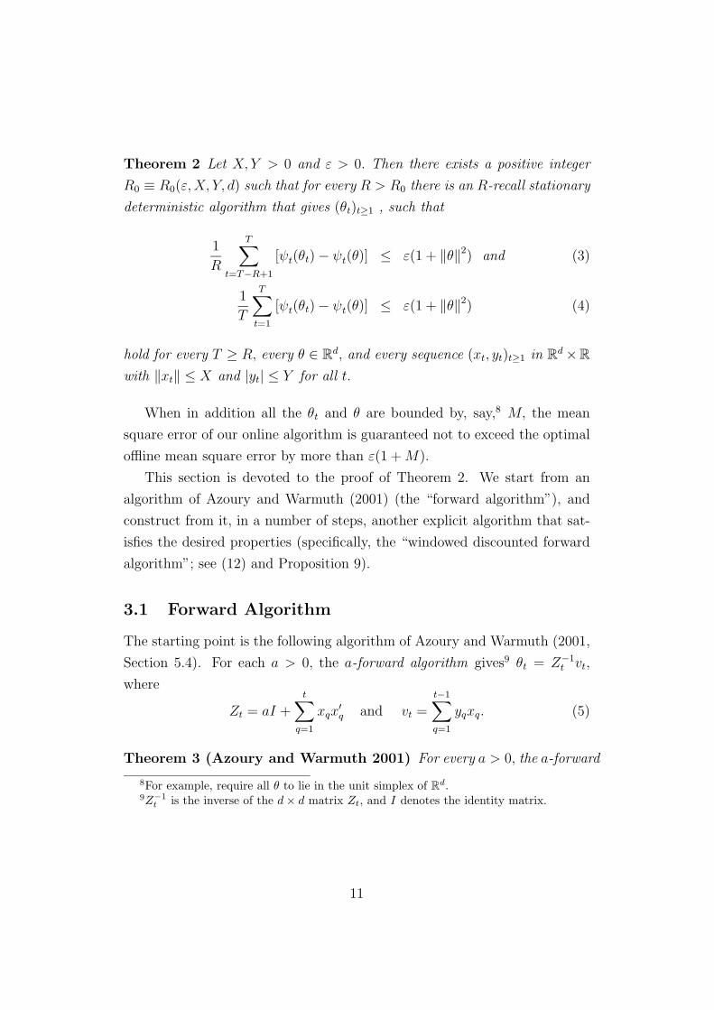
Theorem 2 Let X,Y > 0 and ε > 0. Then there exists a positive integer

R0 ≡ R0(ε,X, Y, d) such that for every R > R0 there is an R-recall stationary

deterministic algorithm that gives (θt)t≥1 , such that

1

R

T∑

t=T−R+1

[ψt(θt) − ψt(θ)] ≤ ε(1 + ‖θ‖2) and (3)

1

T

T∑

t=1

[ψt(θt) − ψt(θ)] ≤ ε(1 + ‖θ‖2) (4)

hold for every T ≥ R, every θ ∈ Rd, and every sequence (xt, yt)t≥1 in R

d ×R

with ‖xt‖ ≤ X and |yt| ≤ Y for all t.

When in addition all the θt and θ are bounded by, say,8 M, the mean

square error of our online algorithm is guaranteed not to exceed the optimal

offline mean square error by more than ε(1 + M).

This section is devoted to the proof of Theorem 2. We start from an

algorithm of Azoury and Warmuth (2001) (the “forward algorithm”), and

construct from it, in a number of steps, another explicit algorithm that sat-

isfies the desired properties (specifically, the “windowed discounted forward

algorithm”; see (12) and Proposition 9).

3.1 Forward Algorithm

The starting point is the following algorithm of Azoury and Warmuth (2001,

Section 5.4). For each a > 0, the a-forward algorithm gives9 θt = Z−1t vt,

where

Zt = aI +t

∑

q=1

xqx′q and vt =

t−1∑

q=1

yqxq. (5)

Theorem 3 (Azoury and Warmuth 2001) For every a > 0, the a-forward

8For example, require all θ to lie in the unit simplex of Rd.

9Z−1t is the inverse of the d × d matrix Zt, and I denotes the identity matrix.

11

algorithm yields

T∑

t=1

ψt(θt) − minθ∈Rd

(

a ‖θ‖2 +T

∑

t=1

ψt(θ)

)

≤T

∑

t=1

y2t

(

1 − det(Zt−1)

det(Zt)

)

(6)

for every T ≥ 1 and every sequence (xt, yt)t≥1 in Rd × R.

Proof. Theorem 5.6 and Lemma A.1 in Azoury and Warmuth (2001), where

Zt denotes their η−1t matrix; the second term in their formula (5.17) is non-

negative since ηt is a positive definite matrix.10 ¤

3.2 Discounted Forward Algorithm

Let a > 0 and 0 < λ < 1. The λ-discounted a-forward algorithm gives

θt = Z−1t vt, where

Zt = aI +t

∑

q=1

λt−qxqx′q and vt =

t−1∑

q=1

λt−qyqxq. (7)

Proposition 4 For every a > 0 and 0 < λ < 1, the λ-discounted a-forward

algorithm yields

T∑

t=1

λT−t [ψt(θt) − ψt(θ)] ≤ a ‖θ‖2 +T

∑

t=1

λT−ty2t

(

1 − λd det(Zt−1)

det(Zt)

)

(8)

for every T ≥ 1, every θ ∈ Rd, and every sequence (xt, yt)t≥1 in R

d × R.

Proof. Let b :=√

a(1 − λ). From the sequence (xt, yt)t≥1 we construct a

sequence (xs, ys)s≥1 in blocks as follows. For every t ≥ 1, the t-th block Bt is

of size d+1 and consists of (λ−t/2be(1), 0), ..., (λ−t/2be(d), 0), (λ−t/2xt, λ−t/2yt),

where e(i) is the i-th unit vector in Rd. The a-forward algorithm applied to

(xs, ys)s≥1 yields the following.

10Our statement is different from theirs because ψt equals twice Lt, and there is amisprinted sign in the first line of their formula (5.17).

12

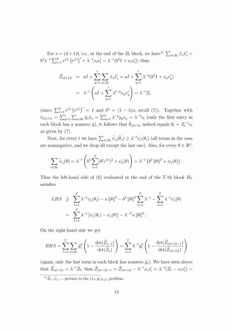
For s = (d + 1)t, i.e., at the end of the Bt block, we have11∑

s∈Btxsx

′s =

b2λ−t ∑di=1 e(i)

(

e(i))′

+ λ−txtx′t = λ−t(b2I + xtx

′t); thus

Z(d+1)t = aI +t

∑

q=1

∑

s∈Bt

xsx′s = aI +

t∑

q=1

λ−q(b2I + xqx′q)

= λ−t

(

aI +t

∑

q=1

λt−qxqx′q

)

= λ−tZt

(since∑d

i=1 e(i)(

e(i))′

= I and b2 = (1 − λ)a; recall (7)). Together with

v(d+1)t =∑t

q=1

∑

s∈Btysxs =

∑tq=1 λ−qyqxq = λ−tvt (only the first entry in

each block has a nonzero y), it follows that θ(d+1)t indeed equals θt = Z−1t vt

as given by (7).

Next, for every t we have∑

s∈Btψs(θs) ≥ λ−tψt(θt) (all terms in the sum

are nonnegative, and we drop all except the last one). Also, for every θ ∈ Rd,

∑

s∈Bt

ψs(θ) = λ−t

(

b2

d∑

i=1

(θ′e(i))2 + ψt(θ)

)

= λ−t(

b2 ‖θ‖2 + ψt(θ))

.

Thus the left-hand side of (6) evaluated at the end of the T -th block BT

satisfies

LHS ≥T

∑

t=1

λ−tψt(θt) − a ‖θ‖2 − b2 ‖θ‖2T

∑

t=1

λ−t −T

∑

t=1

λ−tψt(θ)

=T

∑

t=1

λ−t [ψt(θt) − ψt(θ)] − λ−T a ‖θ‖2 .

On the right-hand side we get

RHS =T

∑

t=1

∑

s∈Bt

y2s

(

1 − det(Zs−1)

det(Zs)

)

=T

∑

t=1

λ−ty2t

(

1 − det(Z(d+1)t−1)

det(Z(d+1)t)

)

(again, only the last term in each block has nonzero ys). We have seen above

that Z(d+1)t = λ−tZt; thus Z(d+1)t−1 = Z(d+1)t − λ−txtx′t = λ−t(Zt − xtx

′t) =

11Zs, ψs, ... pertain to the (xs, ys)s≥1 problem.

13

λ−t+1Zt−1 + (λ−t − λ−t+1)aI. Therefore det(Z(d+1)t−1) ≥ det(λ−t+1Zt−1) (in-

deed, if B is a positive definite matrix and β > 0 then12 det(B + βI) >

det(B)). Therefore we obtain

RHS ≤T

∑

t=1

λ−ty2t

(

1 − det(λ−t+1Zt−1)

det(λ−tZt)

)

=T

∑

t=1

λ−ty2t

(

1 − λd det(Zt−1)

det(Zt)

)

(the matrices Zt are of size d × d, and so det(cZt) = cd det(Zt)). Recalling

that LHS ≤ RHS by (6) and multiplying by λT yields the result. ¤

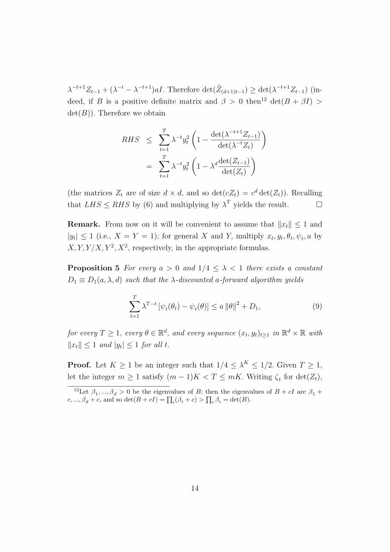
Remark. From now on it will be convenient to assume that ‖xt‖ ≤ 1 and

|yt| ≤ 1 (i.e., X = Y = 1); for general X and Y, multiply xt, yt, θt, ψt, a by

X,Y, Y/X, Y 2, X2, respectively, in the appropriate formulas.

Proposition 5 For every a > 0 and 1/4 ≤ λ < 1 there exists a constant

D1 ≡ D1(a, λ, d) such that the λ-discounted a-forward algorithm yields

T∑

t=1

λT−t [ψt(θt) − ψt(θ)] ≤ a ‖θ‖2 + D1, (9)

for every T ≥ 1, every θ ∈ Rd, and every sequence (xt, yt)t≥1 in R

d × R with

‖xt‖ ≤ 1 and |yt| ≤ 1 for all t.

Proof. Let K ≥ 1 be an integer such that 1/4 ≤ λK ≤ 1/2. Given T ≥ 1,

let the integer m ≥ 1 satisfy (m − 1)K < T ≤ mK. Writing ζt for det(Zt),

12Let β1, ..., βd > 0 be the eigenvalues of B; then the eigenvalues of B + cI are β1 +c, ..., βd + c, and so det(B + cI) =

∏

i(βi + c) >∏

i βi = det(B).

14

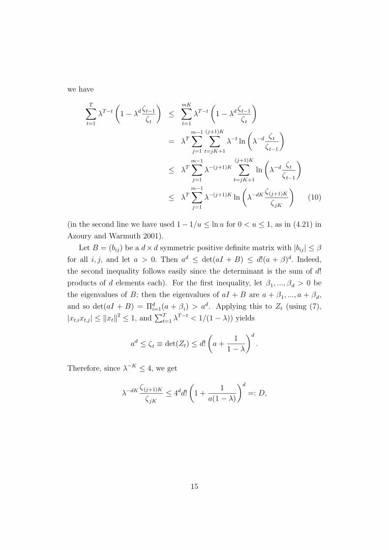
we have

T∑

t=1

λT−t

(

1 − λd ζt−1

ζt

)

≤mK∑

t=1

λT−t

(

1 − λd ζt−1

ζt

)

= λTm−1∑

j=1

(j+1)K∑

t=jK+1

λ−t ln

(

λ−d ζt

ζt−1

)

≤ λTm−1∑

j=1

λ−(j+1)K

(j+1)K∑

t=jK+1

ln

(

λ−d ζt

ζt−1

)

≤ λTm−1∑

j=1

λ−(j+1)K ln

(

λ−dKζ(j+1)K

ζjK

)

(10)

(in the second line we have used 1− 1/u ≤ ln u for 0 < u ≤ 1, as in (4.21) in

Azoury and Warmuth 2001).

Let B = (bij) be a d× d symmetric positive definite matrix with |bij| ≤ β

for all i, j, and let a > 0. Then ad ≤ det(aI + B) ≤ d!(a + β)d. Indeed,

the second inequality follows easily since the determinant is the sum of d!

products of d elements each). For the first inequality, let β1, ..., βd > 0 be

the eigenvalues of B; then the eigenvalues of aI + B are a + β1, ..., a + βd,

and so det(aI + B) = Πdi=1(a + βi) > ad. Applying this to Zt (using (7),

|xt,ixt,j| ≤ ‖xt‖2 ≤ 1, and∑T

t=1 λT−t < 1/(1 − λ)) yields

ad ≤ ζt ≡ det(Zt) ≤ d!

(

a +1

1 − λ

)d

.

Therefore, since λ−K ≤ 4, we get

λ−dKζ(j+1)K

ζjK

≤ 4dd!

(

1 +1

a(1 − λ)

)d

=: D,

15

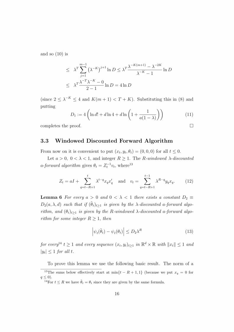
and so (10) is

≤ λTm−1∑

j=1

(

λ−K)j+1

ln D ≤ λT λ−K(m+1) − λ−2K

λ−K − 1ln D

≤ λT λ−T λ−K − 0

2 − 1ln D = 4 ln D

(since 2 ≤ λ−K ≤ 4 and K(m + 1) < T + K). Substituting this in (8) and

putting

D1 := 4

(

ln d! + d ln 4 + d ln

(

1 +1

a(1 − λ)

))

(11)

completes the proof. ¤

3.3 Windowed Discounted Forward Algorithm

From now on it is convenient to put (xt, yt, θt) = (0, 0, 0) for all t ≤ 0.

Let a > 0, 0 < λ < 1, and integer R ≥ 1. The R-windowed λ-discounted

a-forward algorithm gives θt = Z−1t vt, where13

Zt = aI +t

∑

q=t−R+1

λt−qxqx′q and vt =

t−1∑

q=t−R+1

λR−qyqxq. (12)

Lemma 6 For every a > 0 and 0 < λ < 1 there exists a constant D2 ≡D2(a, λ, d) such that if (θt)t≥1 is given by the λ-discounted a-forward algo-

rithm, and (θt)t≥1 is given by the R-windowed λ-discounted a-forward algo-

rithm for some integer R ≥ 1, then

∣

∣

∣ψt(θt) − ψt(θt)

∣

∣

∣≤ D2λ

R (13)

for every14 t ≥ 1 and every sequence (xt, yt)t≥1 in Rd × R with ‖xt‖ ≤ 1 and

|yt| ≤ 1 for all t.

To prove this lemma we use the following basic result. The norm of a

13The sums below effectively start at mint − R + 1, 1 (because we put xq = 0 forq ≤ 0).

14For t ≤ R we have θt = θt since they are given by the same formula.

16

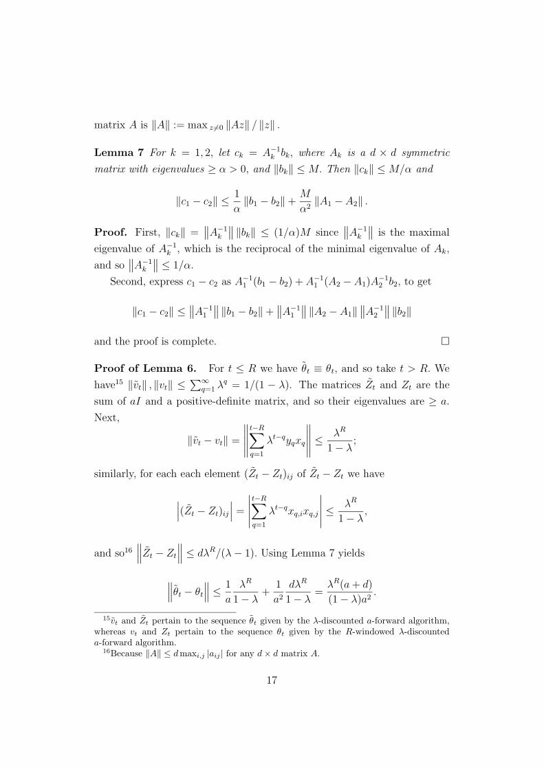
matrix A is ‖A‖ := max z 6=0 ‖Az‖ / ‖z‖ .

Lemma 7 For k = 1, 2, let ck = A−1k bk, where Ak is a d × d symmetric

matrix with eigenvalues ≥ α > 0, and ‖bk‖ ≤ M. Then ‖ck‖ ≤ M/α and

‖c1 − c2‖ ≤ 1

α‖b1 − b2‖ +

M

α2‖A1 − A2‖ .

Proof. First, ‖ck‖ =∥

∥A−1k

∥

∥ ‖bk‖ ≤ (1/α)M since∥

∥A−1k

∥

∥ is the maximal

eigenvalue of A−1k , which is the reciprocal of the minimal eigenvalue of Ak,

and so∥

∥A−1k

∥

∥ ≤ 1/α.

Second, express c1 − c2 as A−11 (b1 − b2) + A−1

1 (A2 − A1)A−12 b2, to get

‖c1 − c2‖ ≤∥

∥A−11

∥

∥ ‖b1 − b2‖ +∥

∥A−11

∥

∥ ‖A2 − A1‖∥

∥A−12

∥

∥ ‖b2‖

and the proof is complete. ¤

Proof of Lemma 6. For t ≤ R we have θt ≡ θt, and so take t > R. We

have15 ‖vt‖ , ‖vt‖ ≤ ∑∞

q=1 λq = 1/(1 − λ). The matrices Zt and Zt are the

sum of aI and a positive-definite matrix, and so their eigenvalues are ≥ a.

Next,

‖vt − vt‖ =

∥

∥

∥

∥

∥

t−R∑

q=1

λt−qyqxq

∥

∥

∥

∥

∥

≤ λR

1 − λ;

similarly, for each each element (Zt − Zt)ij of Zt − Zt we have

∣

∣

∣(Zt − Zt)ij

∣

∣

∣=

∣

∣

∣

∣

∣

t−R∑

q=1

λt−qxq,ixq,j

∣

∣

∣

∣

∣

≤ λR

1 − λ,

and so16∥

∥

∥Zt − Zt

∥

∥

∥≤ dλR/(λ − 1). Using Lemma 7 yields

∥

∥

∥θt − θt

∥

∥

∥≤ 1

a

λR

1 − λ+

1

a2

dλR

1 − λ=

λR(a + d)

(1 − λ)a2.

15vt and Zt pertain to the sequence θt given by the λ-discounted a-forward algorithm,whereas vt and Zt pertain to the sequence θt given by the R-windowed λ-discounteda-forward algorithm.

16Because ‖A‖ ≤ d maxi,j |aij | for any d × d matrix A.

17

Hence

∣

∣

∣ψt(θt) − ψt(θt)

∣

∣

∣=

∣

∣

∣(yt − θ

′

txt)2 − (yt − θ′txt)

2∣

∣

∣

=∣

∣

∣(θ

′

t − θ′t)xt ·(

2yt − (θ′

t + θ′t)xt

)∣

∣

∣

≤∥

∥

∥θt − θt

∥

∥

∥

(

2 +∥

∥

∥θt

∥

∥

∥+ ‖θt‖

)

≤ λR(a + d)

(1 − λ)a2

(

2 +2

(1 − λ)a

)

= D2λR,

where

D2 :=2 (a + d) (a(1 − λ) + 1)

a3(1 − λ)2; (14)

this completes the proof. ¤

Proposition 8 For every a > 0 and 1/4 ≤ λ < 1 there exist constants

D1 ≡ D1(a, λ, d) and D2 ≡ D2(a, λ, d) such that for every integer R ≥ 1 the

R-windowed λ-discounted a-forward algorithm yields

1

R

T∑

t=T−R+1

[ψt(θt) − ψt(θ)] ≤ (a ‖θ‖2 + D1)

(

1 − λ +λ

R

)

(15)

+(‖θ‖ + 1)2

R(1 − λ)+ D2λ

R

for every T ≥ 1, every θ ∈ Rd, and every sequence (xt, yt)t≥1 in R

d × R with

‖xt‖ ≤ 1 and |yt| ≤ 1 for all t.

Proof. Let θt be given by the λ-discounted a-forward algorithm. Put gt :=

ψt(θt)− ψt(θ) (where θt is given by the R-windowed λ-discounted a-forward

algorithm) and gt := ψt(θt) − ψt(θ). Apply (9) at T, and also at each one of

T −R + 1, T −R + 2, ..., T − 1; multiply those by 1− λ and add them all, to

get

T∑

t=1

λT−tgt + (1 − λ)R−1∑

r=1

T−r∑

t=1

λT−r−tgt ≤ (a ‖θ‖2 + D1)(1 + (R − 1)(1 − λ))

= (a ‖θ‖2 + D1)(R − Rλ + λ).

18

For t ≤ T − R, the total coefficient of gt on the left-hand side above is

λT−t + (1 − λ)∑R−1

r=1 λT−r−t = λT−R+1−t; for T − R + 1 ≤ t ≤ T, it is

λT−t + (1 − λ)∑T−t

r=1 λT−r−t = 1. Therefore

T−R∑

t=1

λT−R+1−tgt +T

∑

t=T−R+1

gt ≤ (a ‖θ‖2 + D1)(R − Rλ + λ).

Now gt ≥ −ψt(θ) ≥ −(‖θ‖ ‖xt‖ + |yt|)2 ≥ −(‖θ‖ + 1)2, and so

T∑

t=T−R+1

gt ≤ (a ‖θ‖2 + D1)(R − Rλ + λ) + (‖θ‖ + 1)2

T−R∑

t=1

λT−R+1−t

≤ (a ‖θ‖2 + D1)(R − Rλ + λ) +(‖θ‖ + 1)2

1 − λ.

Divide by R and use gt ≤ gt + D2λR (by Proposition 6). ¤

Choosing appropriate λ and R allows us to bound the right-hand side of

(15).

Proposition 9 For every ε > 0 and a > 0 there is λ0 ≡ λ0(ε, a, d) < 1 such

that for every λ0 < λ < 1 there is R0 ≡ R0(ε, a, d, λ) ≥ 1 such that for every

R ≥ R0 the R-windowed λ-discounted a-forward algorithm yields

1

R

T∑

t=T−R+1

[ψt(θt) − ψt(θ)] ≤ ε(1 + ‖θ‖2), (16)

1

T

T∑

t=1

[ψt(θt) − ψt(θ)] ≤ ε(1 + ‖θ‖2), (17)

for every T ≥ R, every θ ∈ Rd, and every sequence (xt, yt)t≥1 in R

d ×R with

‖xt‖ ≤ 1 and |yt| ≤ 1 for all t.

Proof. The right-hand side of (15) is

≤(

D1(1 − λ) +D1

R+

2

R(1 − λ)+ D2λ

R

)

+‖θ‖2

(

a(1 − λ) +a

R+

2

R(1 − λ)

)

19

(use λ/R ≤ 1/R and (‖θ‖ + 1)2 ≤ 2 ‖θ‖2 + 2). First, take 1/4 ≤ λ0 < 1

close enough to 1 so that a(1 − λ0) ≤ ε/4 and D1(a, λ0, d) · (1 − λ0) ≤ ε/4

(recall formula (11) for D1 and use limx→0+ x ln x = 0). Then, given λ ∈[λ0, 1), take R0 ≥ 1 large enough so that a/R0 ≤ ε/4, D1(a, λ, d)/R0 ≤ ε/4,

2/(R0(1 − λ)) ≤ ε/4, and D2(a, λ, d)λR0 ≤ ε/4. This shows (16) for every

T ≥ 1.

In particular, for T ′ < R we get (1/R)∑T ′

t=1 [ψt(θt) − ψt(θ)] ≤ ε(1+‖θ‖2)

(because (xt, yt, θt) = (0, 0, 0) for all t ≤ 0). For T ≥ R, add inequality

(16) for the disjoint blocks of size R that end at t = T, together with the

above inequality for the initial smaller block of size T ′ < R when T is not

a multiple of R, to get (1/R)∑T

t=1 [ψt(θt) − ψt(θ)] ≤ ⌈T/R⌉ε(1 + ‖θ‖2) ≤2(T/R)ε(1 + ‖θ‖2). Replacing ε with ε/2 yields (17). ¤

Remark. Similar arguments show that, for λ0 ≤ λ < 1, the discounted

average is also small:

1 − λ

1 − λT

T∑

t=1

λT−t [ψt(θt) − ψt(θ)] ≤ ε(1 + ‖θ‖2).

Proposition 9 yields the main result of this section, Theorem 2.

Proof of Theorem 2. Use Proposition 9 (with, say, a = 1), and rescale

everything by X and Y appropriately (see the Remark before Proposition

5). ¤

4 Weak Calibration

The notion of “weak calibration” was introduced by Kakade and Foster

(2004) and Foster and Kakade (2006). The idea is as follows. Given a “test”

function w : C → 0, 1 that indicates which forecasts c to consider, let the

corresponding score be17 SwT := ||(1/T )

∑Tt=1 w(ct)(at − ct)||. It can be shown

17The ST scores are norms of averages, rather than averages of norms like the KT scores.“Windowed” versions of the scores may also be considered (with the average taken overthe last R periods only; cf. (3)).

20

that if SwT is small for every such w, then the calibration score KT is also

small.18

Now instead of the discontinuous indicator functions, weak calibration

requires that SwT be small for continuous “weight” functions w : C → [0, 1].

Specifically, let ε > 0 and L < ∞. A procedure (i.e., a strategy of the C-player

in the calibration game) is (ε, L)-weakly calibrated if there is T0 ≡ T0(ε, L)

such that

SwT =

∥

∥

∥

∥

∥

1

T

T∑

t=1

w(ct)(at − ct)

∥

∥

∥

∥

∥

≤ ε (18)

holds for every strategy of the A-player, every T > T0, and every weight

function w : C → [0, 1] that is L-Lipschitz (i.e., L(w) ≤ L).

The importance of weak calibration is that, unlike regular calibration,

it can be guaranteed by deterministic procedures (which are thus leaky):

Kakade and Foster (2004) and Foster and Kakade (2006) have proven the

existence of deterministic (ε, L)-weakly calibrated procedures. Moreover, as

we will show in the next section, weak calibration is essentially equivalent to

smooth calibration.

We now provide a deterministic (ε, L)-weakly calibrated procedure that

in addition has finite recall and is stationary.

Theorem 10 For every ε > 0 and L < ∞ there exists an (ε, L)-weakly cal-

ibrated deterministic procedure that has finite recall and is stationary; more-

over, all its forecasts may be taken to lie on a finite grid.

Proof. Without loss of generality assume that A ⊆ C ⊆ [0, 1]m (one can

always translate the sets A and C—which does not affect (18)—and rescale

them—which just rescales the Lipschitz constant); assume also that L ≥ 1

(as L increases there are more Lipschitz functions) and ε ≤ 1.

18Specifically, if SwT ≤ ε for all w : C → 0, 1 then KT ≤ 2mε. Indeed, for each

coordinate i = 1, ...,m, let Ci+ be the set of all ct such that at,i > ct,i, and Ci

− the set of all ct

such that at,i < ct,i. Taking w to be the indicator of Ci+ yields Sw

T = (1/T )∑

t[at,i−ct,i]+ ≤ε (where [z]+ := maxz, 0); similarly, the indicator of Ci

− yields (1/T )∑

t[at,i−ct,i]− ≤ ε.Adding the two inequalities gives (1/T )

∑

t |at,i − ct,i| ≤ 2ε. Since this holds for each oneof the m coordinates, it follows that KT ≤ 2mε.

21

For every b ∈ Rm let γ(b) := arg minc∈C ‖c − b‖ be the closest point to b

in C (it is well defined and unique since C is a convex compact set); then

‖c − b‖ ≥ ‖c − γ(b)‖ (19)

for every c ∈ C (because ‖c − b‖2 = ‖c − γ(b)‖2 + ‖b − γ(b)‖2 − 2(b− γ(b)) ·(c − γ(b)) and the third term is ≤ 0).

Let ε1 := ε/(2√

m). Denote by WL the set of weight functions w : C →[0, 1] with L(w) ≤ L. By Lemma 16 in the Appendix, for every w ∈ WL there

is a vector ≡ w ∈ [0, 1]d such that19

maxc∈C

∣

∣

∣

∣

∣

w(c) −d

∑

i=1

ifi(c)

∣

∣

∣

∣

∣

≤ ε1. (20)

Denote F (c) := (f1(c), ..., fd(c)) ∈ [0, 1]d; thus ‖F (c)‖ ≤√

d. Without loss

of generality we assume that the coordinate functions are included in the set

f1, ..., fd, say, fj(c) = cj for j = 1, ...,m (thus d > m, in fact d is much

larger than m).

Let ε2 := ε/(m + m(1 + d)2 + d2) (where d is given above, and depends

on ε,m, and L) and ε3 := (ε2)2.

Let λ and R be given by Theorem 2 and Proposition 9 for a = 1, X =√

d,

Y = 1, and ε = ε3. For each j = 1, ...,m consider the sequence (xt, y(j)t )t≥1 =

(F (ct), at,j)t≥1 in Rd × R, where at ∈ A is determined by the A-player, and

ct ∈ C is constructed inductively as follows.

19Since WL is compact in the sup norm, there are f1, ..., fd ∈ WL such that for everyw ∈ WL there is 1 ≤ i ≤ d with maxc∈C |w(c) − fi(c)| ≤ ε1. Lemma 16 improves this, ingetting a much smaller d by using linear combinations with bounded coefficients.

22

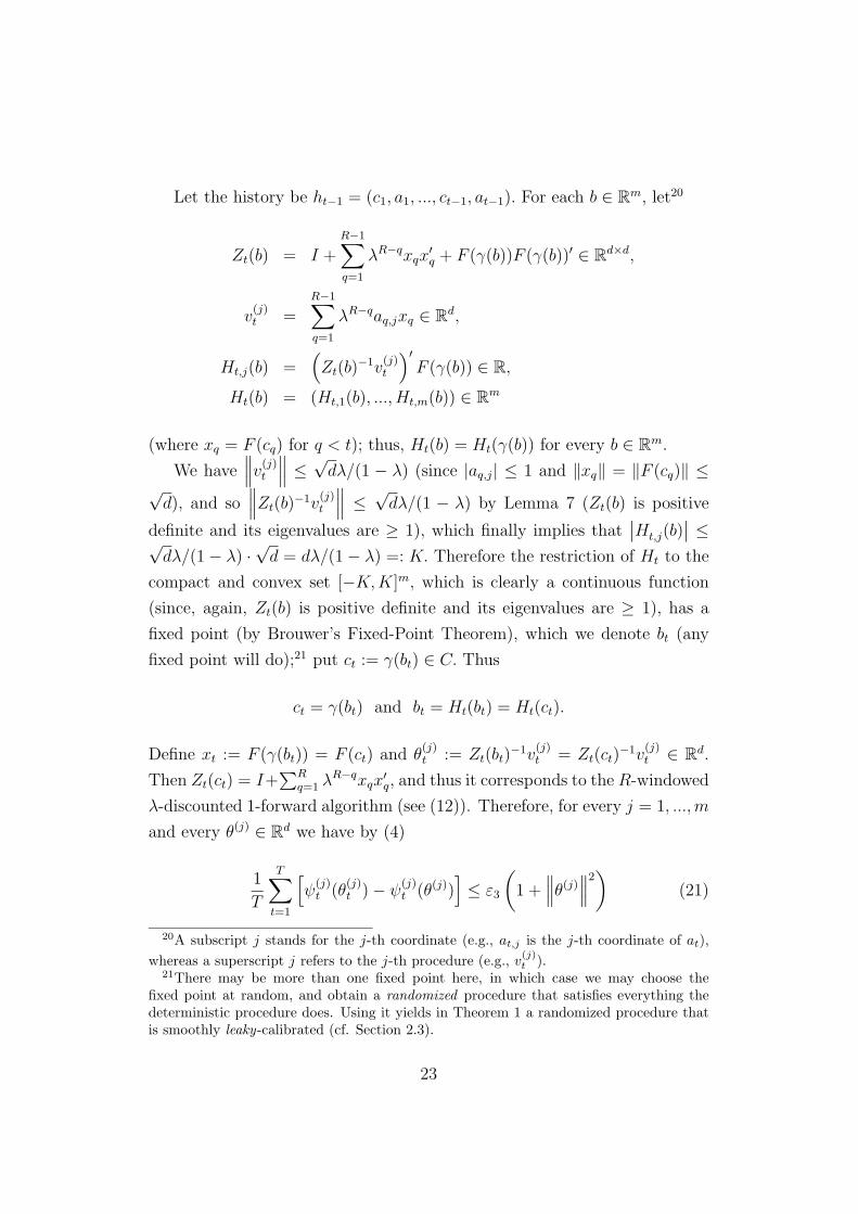
Let the history be ht−1 = (c1, a1, ..., ct−1, at−1). For each b ∈ Rm, let20

Zt(b) = I +R−1∑

q=1

λR−qxqx′q + F (γ(b))F (γ(b))′ ∈ R

d×d,

v(j)t =

R−1∑

q=1

λR−qaq,jxq ∈ Rd,

Ht,j(b) =(

Zt(b)−1v

(j)t

)′

F (γ(b)) ∈ R,

Ht(b) = (Ht,1(b), ..., Ht,m(b)) ∈ Rm

(where xq = F (cq) for q < t); thus, Ht(b) = Ht(γ(b)) for every b ∈ Rm.

We have∥

∥

∥v

(j)t

∥

∥

∥≤

√dλ/(1 − λ) (since |aq,j| ≤ 1 and ‖xq‖ = ‖F (cq)‖ ≤

√d), and so

∥

∥

∥Zt(b)

−1v(j)t

∥

∥

∥≤

√dλ/(1 − λ) by Lemma 7 (Zt(b) is positive

definite and its eigenvalues are ≥ 1), which finally implies that∣

∣Ht,j(b)∣

∣ ≤√dλ/(1 − λ) ·

√d = dλ/(1 − λ) =: K. Therefore the restriction of Ht to the

compact and convex set [−K,K]m, which is clearly a continuous function

(since, again, Zt(b) is positive definite and its eigenvalues are ≥ 1), has a

fixed point (by Brouwer’s Fixed-Point Theorem), which we denote bt (any

fixed point will do);21 put ct := γ(bt) ∈ C. Thus

ct = γ(bt) and bt = Ht(bt) = Ht(ct).

Define xt := F (γ(bt)) = F (ct) and θ(j)t := Zt(bt)

−1v(j)t = Zt(ct)

−1v(j)t ∈ R

d.

Then Zt(ct) = I+∑R

q=1 λR−qxqx′q, and thus it corresponds to the R-windowed

λ-discounted 1-forward algorithm (see (12)). Therefore, for every j = 1, ...,m

and every θ(j) ∈ Rd we have by (4)

1

T

T∑

t=1

[

ψ(j)t (θ

(j)t ) − ψ

(j)t (θ(j))

]

≤ ε3

(

1 +∥

∥

∥θ(j)

∥

∥

∥

2)

(21)

20A subscript j stands for the j-th coordinate (e.g., at,j is the j-th coordinate of at),

whereas a superscript j refers to the j-th procedure (e.g., v(j)t ).

21There may be more than one fixed point here, in which case we may choose thefixed point at random, and obtain a randomized procedure that satisfies everything thedeterministic procedure does. Using it yields in Theorem 1 a randomized procedure thatis smoothly leaky-calibrated (cf. Section 2.3).

23

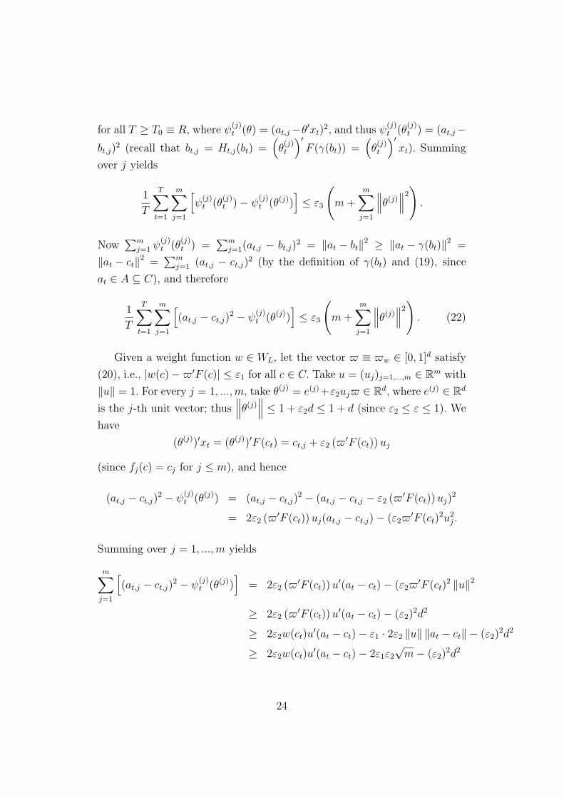
for all T ≥ T0 ≡ R, where ψ(j)t (θ) = (at,j −θ′xt)

2, and thus ψ(j)t (θ

(j)t ) = (at,j −

bt,j)2 (recall that bt,j = Ht,j(bt) =

(

θ(j)t

)′

F (γ(bt)) =(

θ(j)t

)′

xt). Summing

over j yields

1

T

T∑

t=1

m∑

j=1

[

ψ(j)t (θ

(j)t ) − ψ

(j)t (θ(j))

]

≤ ε3

(

m +m

∑

j=1

∥

∥

∥θ(j)

∥

∥

∥

2)

.

Now∑m

j=1 ψ(j)t (θ

(j)t ) =

∑mj=1(at,j − bt,j)

2 = ‖at − bt‖2 ≥ ‖at − γ(bt)‖2 =

‖at − ct‖2 =∑m

j=1 (at,j − ct,j)2 (by the definition of γ(bt) and (19), since

at ∈ A ⊆ C), and therefore

1

T

T∑

t=1

m∑

j=1

[

(at,j − ct,j)2 − ψ

(j)t (θ(j))

]

≤ ε3

(

m +m

∑

j=1

∥

∥

∥θ(j)

∥

∥

∥

2)

. (22)

Given a weight function w ∈ WL, let the vector ≡ w ∈ [0, 1]d satisfy

(20), i.e., |w(c) − ′F (c)| ≤ ε1 for all c ∈ C. Take u = (uj)j=1,...,m ∈ Rm with

‖u‖ = 1. For every j = 1, ...,m, take θ(j) = e(j)+ε2uj ∈ Rd, where e(j) ∈ R

d

is the j-th unit vector; thus∥

∥

∥θ(j)

∥

∥

∥≤ 1 + ε2d ≤ 1 + d (since ε2 ≤ ε ≤ 1). We

have

(θ(j))′xt = (θ(j))′F (ct) = ct,j + ε2 (′F (ct)) uj

(since fj(c) = cj for j ≤ m), and hence

(at,j − ct,j)2 − ψ

(j)t (θ(j)) = (at,j − ct,j)

2 − (at,j − ct,j − ε2 (′F (ct)) uj)2

= 2ε2 (′F (ct)) uj(at,j − ct,j) − (ε2′F (ct)

2u2j .

Summing over j = 1, ...,m yields

m∑

j=1

[

(at,j − ct,j)2 − ψ

(j)t (θ(j))

]

= 2ε2 (′F (ct)) u′(at − ct) − (ε2′F (ct)

2 ‖u‖2

≥ 2ε2 (′F (ct)) u′(at − ct) − (ε2)2d2

≥ 2ε2w(ct)u′(at − ct) − ε1 · 2ε2 ‖u‖ ‖at − ct‖ − (ε2)

2d2

≥ 2ε2w(ct)u′(at − ct) − 2ε1ε2

√m − (ε2)

2d2

24

(since: ‖u‖ = 1, |′F (c)| ≤ d [the coordinates of are between −1 and 1

and those of F (c) between 0 and 1], ‖at − ct‖ ≤ √m (since at, ct ∈ [0, 1]m,

and recall (20)).

Together with (22) we get (recall that ε3 = (ε2)2 and ε1 = ε/(2

√m)):

2ε2 ·1

T

T∑

t=1

w(ct)u′(at − ct) ≤ (ε2)

2(m + m(1 + d)2 + d2) + εε2;

hence, dividing by 2ε2 and recalling that ε2 = ε/(m + m(1 + d)2 + d2)):

u · 1

T

T∑

t=1

w(ct)(at − ct) ≤ε

2+

ε

2= ε.

Since u ∈ Rm with ‖u‖ = 1 was arbitrary, the proof is complete.

For the “moreover” statement, let ε4 := ε/(L√

m + 1), and take D ⊆ C

to be a finite ε4-grid in C; i.e., for every c ∈ C there is d(c) ∈ D with

||d(c) − c|| ≤ ε4. Replace the forecast cT obtained above with cT := d(cT );

then, for every aT ∈ A, we have

||w(cT )(aT − cT ) − w(cT )(aT − cT )|| ≤ Lε4

√m + ε4 = ε.

Therefore the score SwT changes by at most ε, and so it is at most 2ε. ¤

5 Smooth Calibration

In this section we show (Propositions 11 and 12) that weak calibration and

smooth calibration are essentially equivalent (albeit with different constants

ε, L). The existence of weakly calibrated procedures (Theorem 10, proved

in the previous section) then implies the existence of smoothly calibrated

procedures, which proves Theorem 1.

We first show how to go from weak to smooth calibration.

25

Proposition 11 An (ε, L)-weakly calibrated procedure is (ε′, L)-smoothly cal-

ibrated, where22 ε′ = Ω(√

εLm)

.

Proof. Take ε′ :=√

εLm(2√

m)m/2(2 +√

m).

Let (Dj)j=1,...,M be a partition of [0, 1]m ⊇ C into disjoint cubes with side

1/(2L√

m); the diameter of each cube is thus 1/(2L), and the number of

cubes is M = (2L√

m)m.

Fix at, ct ∈ C ⊆ [0, 1]m for t = 1, ..., T, and a smoothing function Λ that is

L-Lipschitz in its first coordinate. Assume that the weak calibaration score

SwT (given by (18)) satisfies Sw

T ≤ ε for every weight function w in WL; we will

show that the smooth calibration score KΛT (given by (1)) satisfies KΛ

T ≤ ε′.

For every t = 1, ..., T, take wt(c) := Λ(c, ct); then wt is a weight function

with L(wt) ≤ L, and so, by our assumption,

∥

∥

∥

∥

∥

T∑

s=1

wt(cs)(as − cs)

∥

∥

∥

∥

∥

≤ Tε. (23)

Now aΛt − cΛ

t =∑T

s=1 wt(cs)(as − cs)/Wt, where Wt :=∑T

s=1 wt(cs), and so

(23) yields∥

∥aΛt − cΛ

t

∥

∥ ≤ Tε1

Wt

. (24)

When Wt is large, (24) provides a good bound; we will show that, for a large

proportion of indices t, this is indeed the case.

Let V ⊆ 1, ..., T be the set of indices t such that the cube Dj that

contains ct includes at least a fraction√

ε1 of c1, ..., cT , i.e., |s ≤ T : cs ∈Dj| ≥ T

√ε1, where ε1 := ε/M. Then wt(cs) ≥ 1/2 for every such cs ∈ Dj

(because ||ct − cs|| ≤ 1/(2L) and so, by the Lipschitz condition, 1−wt(cs) =

wt(ct) − wt(cs) ≤ L||ct − cs|| ≤ 1/2). Therefore Wt ≥ T√

ε1/2 (there are

at least T√

ε such cs, and each one contributes at least 1/2 to the sum

22We have not tried to optimize the estimate of ε′. The notations f(x) = O(g(x)),f(x) = Ω(g(x)), and f(x) = Θ(g(x)) mean, as usual, that there are constants c, c′ > 0 suchthat for all x we have, respectively, f(x) ≤ cg(x), f(x) ≥ c′g(x), and c′g(x) ≤ f(x) ≤ cg(x).In our case x stands for (ε, L); the dimension m is assumed fixed.

26

∑

s wt(cs) = Wt), and so (24) yields

∥

∥aΛt − cΛ

t

∥

∥ ≤ Tε2

T√

ε1

= 2√

Mε (25)

for each t ∈ V. If t /∈ V then ct belongs to one of the cubes Dj that contains

less than T√

ε1 of the c1, ..., cT , and so in total there are no more than M ·T√

ε1 =√

MεT indices t /∈ V. For each one the bound∥

∥aΛt − cΛ

t

∥

∥ ≤ √m

(because both points belong to C ⊆ [0, 1]m) yields

∑

t/∈V

∥

∥aΛt − cΛ

t

∥

∥ ≤√

m√

MεT. (26)

Adding (25) for all t ∈ V together with (26) yields

T∑

t=1

∥

∥aΛt − cΛ

t

∥

∥ ≤ T · 2√

Mε +√

m√

MεT =√

Mε(2 +√

m)T

=√

εLm(2√

m)m/2(2 +√

m)T ≤ ε′T

(because M = (2L√

m)m), and so KΛT ≤ ε′, as claimed. ¤

The existence of smoothly calibrated procedures with the desired prop-

erties follows.

Proof of Theorems 1. Apply Theorem 10 and Proposition 11, and recall

(Section 2.3) that for deterministic procedures leaks do not matter. ¤

Next, we show how to go from smooth to weak calibration.

Proposition 12 An (ε, L)-smoothly calibrated procedure is (ε′, L′)-weakly

calibrated, where23,24 ε′ = Ω(√

εLm)

and L′ = O(√

εLm+2)

.

Proof. Let (Dj)j=1,...,M be a partition of [0, 1]m ⊇ C into disjoint cubes

with side δ := 1/(L√

m); the diameter of each cube is thus δ√

m = 1/L,

and the number of cubes is M = δ−m = Lmmm/2. Let ε1 :=√

εLm and

23Again, we have not tried to optimize the estimates for ε′ and L′.24Thus, given ε′ and L′, one may take L = Θ(L′/ε′) and ε = Θ((ε′)m+2/(L′)m).

27

ε2 := ε1mm/2/M =

√

ε/Lm. Take L′ := Lε1/2 =√

εLm+2/2 and ε′ =

ε1(1 +√

m +√

mm+1) =√

εLm(1 +√

m +√

mm+1).

Fix at, ct ∈ C ⊆ [0, 1]m for t = 1, ..., T, and a weight function w in WL′ .

Assume that KΛT ≤ ε holds for every smoothing function Λ that is L-Lipschitz

in the first coordinate; we will show that SwT ≤ ε′ (where KΛ

T and SwT are given

by (1) and (18), respectively).

Let V ⊆ 1, ..., T be the set of indices t such that the cube Dj that

contains ct includes at least a fraction ε2 of c1, ..., cT , i.e., |s ≤ T : cs ∈Dj| ≥ ε2T. Then

T − |V | = |t ≤ T : t /∈ V | < M · ε2T = ε2MT, (27)

because there are at most M cubes containing less than ε2T points each.

We distinguish two cases.

Case 1 : maxt∈V w(ct) < ε1. Since ||at−ct|| ≤√

m, we have ||∑t∈V w(ct)(at−ct)|| ≤ |V | · ε1 ·

√m ≤ ε1

√mT (use |V | ≤ T ), and ||∑t/∈V w(ct)(at − ct)|| ≤

(T − |V |) · 1 · √m = ε2M√

mT (use (27)). Adding and dividing by T yields

SwT ≤ (ε1 + ε2M)

√m = ε1

√m(1 + mm/2) < Kε1 = ε′.

Case 2 : maxt∈V w(ct) ≥ ε1. Let s ∈ V be such that w(cs) = maxt∈V w(ct) ≥ε1, and let R ⊆ V be the set of indices r such that cr lies in the same cube

Dj as cs.

For each r in R, proceed as follows. First, we have |w(cs) − w(cr)| ≤L′||cs − cr|| ≤ L′ · δ√m = Lε1/2 · (1/L) = ε1/2, and so

w(cr) ≥ w(cs) −ε1

2≥ ε1 −

ε1

2=

ε1

2. (28)

Next, put wr(c) := minw(c), w(cr) and Λ(c, cr) := wr(c)/w(cr) for r ∈R (and, for t /∈ R, put, say, Λ(c, ct) = 1 for all c); then L(Λ(·, cr)) ≤L(w)/w(cr) ≤ L′/(ε1/2) = L, and so, by our assumption

1

T

∑

r∈R

||aΛr − cΛ

r || ≤1

T

∑

t≤T

||aΛt − cΛ

t || ≤ KΛT ≤ ε. (29)

28

We will now show that SwT is close to an appropriate multiple of ||aΛ

r −cΛr ||,

for each r in R. For t in V we have w(ct) ≤ w(cs), and so 0 ≤ w(ct)−wr(ct) ≤w(cs) − w(cr) ≤ ε1/2 (recall (28)), which gives

∥

∥

∥

∥

∥

∑

t∈V

(w(ct) − wr(ct)) (at − ct)

∥

∥

∥

∥

∥

≤ |V | · ε1

2·√

m ≤ 1

2ε1

√mT.

For t /∈ V we have 0 ≤ w(ct) − wr(ct) ≤ 1, and so (recall (27))

∥

∥

∥

∥

∥

∑

t/∈V

(w(ct) − wr(ct)) (at − ct)

∥

∥

∥

∥

∥

≤ (T − |V |) · 1 ·√

m ≤ ε2M√

mT.

Adding the two inequalities and dividing by T yields

SwT =

∥

∥

∥

∥

∥

1

T

T∑

t=1

w(ct)(at − ct)

∥

∥

∥

∥

∥

≤∥

∥

∥

∥

∥

1

T

T∑

t=1

wr(ct)(at − ct)

∥

∥

∥

∥

∥

+√

m(ε1

2+ ε2M

)

≤ ||aΛr − cΛ

r || +√

m(ε1

2+ ε2M

)

,

because∑

t≤T wr(ct)(at−ct) =(∑

t≤T wr(ct))

(aΛr −cΛ

r ) and∑

t≤T wr(ct) ≤ T.

Averaging over all r in the set R, whose size is |R| ≥ ε2T (all points in the

same cube as cs), and then recalling (29), finally gives

SwT ≤ 1

|R|∑

r∈R

||aΛr − cΛ

r || +√

m(ε1

2+ ε2M

)

≤ 1

ε2

1

T

∑

r∈R

||aΛr − cΛ

r || +√

m(ε1

2+ ε2M

)

≤ 1

ε2

ε +√

m(ε1

2+ ε2M

)

=ε√

Lm

√ε

+ ε1

(√m

2+ m(m+1)/2

)

= ε1

(

1 +

√m

2+ m(m+1)/2

)

< Kε1 = ε′,

completing the proof. ¤

29

6 Nash Equilibrium Dynamics

In this section we use our results on smooth calibration to obtain dynamics

in n-person games that are in the long run close to Nash equilibria most of

the time.

A (finite) game is given by a finite set of players N , and, for each player

i ∈ N, a finite set of actions25 Ai and a payoff function ui : A → R, where

A :=∏

i∈N Ai denotes the set of action combinations of all players. The set

of mixed actions of player i is X i := ∆(Ai), which is the unit simplex (i.e.,

the set of probability distributions) on Ai; we identify the pure actions in Ai

with the unit vectors of X i, and so Ai ⊆ X i. Put X :=∏

i∈N X i for the set of

mixed-action combinations. Let C := ∆(A) be the set of joint distributions

on action combinations; thus A ⊆ X ⊆ C ⊆ [0, 1]m, where m =∏

i∈N |Ai|.The payoff functions ui are linearly extended to C, and thus ui : C → R.

For each player i, a combination of mixed actions of the other players

x−i = (xj)j 6=i ∈ ∏

j 6=i Xj =: X−i, and ε ≥ 0, let BRi

ε(x−i) := xi ∈ X i :

ui(xi, x−i) ≥ maxyi∈Xi ui(yi, x−i) − ε denote the set of ε-best replies of i

to x−i. A (mixed) action combination x ∈ X is a Nash ε-equilibrium if

xi ∈ BRiε(x

−i) for every i ∈ N ; let NE(ε) ⊆ X denote the set of Nash

ε-equilibria of the game.

A (discrete-time) dynamic consists of each player i ∈ N playing a pure

action ait ∈ Ai at each time period t = 1, 2, ...; put at = (ai

t)i∈N ∈ A. There

is perfect monitoring: at the end of period t all players observe at. The

dynamic is uncoupled (Hart and Mas-Colell 2003, 2006, 2013) if the play of

every player i may depend only on player i’s payoff function ui (and not on

the other players’ payoff functions). Formally, such a dynamic is given by a

mapping for each player i from the history ht−1 = (a1, ..., at−1) and his own

payoff function ui into X i = ∆(Ai) (player i’s choice may be random); we

will call such mappings uncoupled. Let xit ∈ X i denote the mixed action that

player i plays at time t, and put xt = (xit)i∈N ∈ X.

The dynamics we consider are continuous, smooth variants of the “cali-

25We refer to one-shot choices as “actions” rather than “strategies,” the latter termbeing used for repeated interactions.

30

brated learning” introduced by Foster and Vohra (1997). Calibrated learning

consists of each player best-replying to calibrated forecasts on the other play-

ers’ actions; it results in the joint distribution of play converging in the long

run to the set of correlated equilibria of the game. Kakade and Foster (2004)

defined publicly calibrated learning, where each player approximately best-

replies to a public weakly calibrated forecast on all players’ actions, and

proved that most of the time the play is an approximate Nash equilibrium.

We consider instead smooth calibrated learning, where weak calibration is

replaced with the more natural smooth calibration; it amounts to taking cal-

ibrated learning and smoothing out both the forecasts and the best replies.

Formally, a smooth calibrated learning dynamic is given by:

(D1) An (εc, Lc)-smoothly calibrated deterministic procedure, which yields

at time t a “forecast” ct ∈ C.

(D2) An Lg-Lipschitz εg-approximate best-reply mapping g : C → ∏

i∈N ∆(Ai);

i.e., gi(c) ∈ BRiεg

(c−i) for every i ∈ N and26 c−i ∈ ∆(A−i), g(c) =

(gi(c))i∈N , and L(g) ≤ Lg.

(D3) Each player runs the procedure in (D1), generating at time t a forecast

ct ∈ C; then each player i plays at period t the mixed action27 xit :=

gi(ct) ∈ ∆(Ai), where gi is given by (D2). All players observe the

action combination at = (ait)i∈N ∈ A that has actually been played,

and remember it together with the forecast28 ct ∈ C.

Smooth calibrated learning is a stochastic uncoupled dynamic: stochastic

because the players use mixed actions, and uncoupled because the payoff

26For a joint distribution c ∈ C = ∆(A) on action combinations and a player i, wedenote by c−i ∈ ∆(A−i) the marginal of c on A−i (when x = (xi)i∈N ∈ ∏

i∈N ∆(Ai) is aproduct distribution then x−i = (xj)j 6=i ∈

∏

j 6=i ∆(Aj)). The ε-best-reply correspondence

BRiε is defined also for c−i ∈ ∆(A−i), i.e., BRi

ε(c−i) := xi ∈ ∆(Ai) : ui(xi, c−i) ≥

maxyi∈∆(Ai) ui(yi, c−i) − ε, where (yi, c−i) denotes the product of the two distributions,yi (on Ai) and c−i (on A−i).

27Thus P [at = a | ht−1] =∏

i∈N xit(a

i) for every a = (ai)i∈N ∈ A, where ht−1 is thehistory and xi

t(ai) is the probability that xi

t ∈ ∆(Ai) assigns to the pure action ai ∈ Ai.28As we will see below, it suffices to remember the actions and forecasts of the last R

periods only (for an appropriate finite R).

31

function of player i is used by player i only, in constructing his approximate

best-reply mapping gi.

Our result is:

Theorem 13 Fix the finite set of players N, the finite action spaces Ai for

all i ∈ N, and the payoff bound U < ∞. For every ε > 0 there exist stochas-

tic uncoupled dynamics—e.g., smooth calibrated learning—that have finite

memory and are stationary, such that

lim infT→∞

1

T|t ≤ T : xt ∈ NE(ε)| ≥ 1 − ε (a.s.)

for every finite game with payoff functions (ui)i∈N that are bounded by U

(i.e., |ui(a)| ≤ U for all i ∈ N and a ∈ A).

The idea of the proof is as follows. First, assume that the forecasts ct

are in fact calibrated (rather than just smoothly calibrated) and, moreover,

that they are calibrated with respect to the mixed plays xt (rather than with

respect to the actual plays at). Because xt is given by a fixed function of ct,

namely, xt = g(ct), the sequence of mixed plays in those periods when the

forecast was a certain c is the constant sequence g(c), ..., g(c), whose average

is g(c), and calibration then implies that g(c) must be close to c (most of

the time, i.e., for forecasts that appear with positive frequency). But we

have only smooth calibration; however, because g is a Lipschitz function,

if c and g(c) are far from one another then so are c′ and g(c′) for any c′

close to c, and so the average of such g(c′) is also far from c, contradicting

smooth calibration. Thus, most of the time g(ct) is close to ct, and hence

g(g(ct)) is close to g(ct) (because g is Lipschitz)—which says that g(ct) is close

to an approximate best reply to itself, i.e., g(ct) is an approximate Nash

equilibrium. Finally, an appropriate use of a strong law of large numbers

shows that if the actual plays at are (smoothly) calibrated then so are their

expectations, i.e., the mixed plays xt.

Proof. This proof goes along similar lines to the proof of Kakade and Foster

32

(2004) for publicly calibrated dynamics (which is the only other calibration-

based Nash dynamic to date29).

The existence of a deterministic smoothly calibrated procedure is given

by Theorem 1, and that of a Lipschitz approximate best-reply mapping is

given by Lemma 17 in the Appendix (the function ui is linear in ci, and

|ui(a)| ≤ U for all a ∈ A implies that L(ui) ≤ 2√

mU =: Lu). For each

period t, let ct ∈ C be the forecast, xt = g(ct) ∈∏

i∈N ∆(Ai) the mixed

actions, and at ∈ A the realized pure actions (ct, xt, and at all depend on the

history).

Let W be the set of weight functions w : C → [0, 1] with L(w) ≤ Lc, and

let w1, ..., wK ∈ W be an30 ε1-net of W. From31E [at | ht−1] = xt = g(ct) it

follows that E [wk(ct)at | ht−1] = wk(ct)g(ct) for every k = 1, ..., K, and hence,

by the Strong Law of Large Numbers for Dependent Random Variables (see

Loeve 1978, Theorem 32.1.E: (1/T )∑T

t=1(Xt − E [Xt|ht−1]) → 0 as T → ∞a.s., for random variables Xt that are, in particular, uniformly bounded; note

that there are finitely many k):

limT→∞

1

T

T∑

t=1

wk(ct)(at − g(ct)) = 0 for all 1 ≤ k ≤ K (a.s.). (30)

Thus, for each one of the (almost all) infinite histories h∞ where (30)

holds, there is a finite T1 (depending on h∞) such that∥

∥

∥

∑Tt=1 wk(ct)(at − g(ct))

∥

∥

∥≤

ε1T for all T > T1 and all 1 ≤ k ≤ K; since the wk constitute an ε1-net of

W and ||c|| ≤ √m for every c ∈ C, it follows that

∥

∥

∥

∥

∥

T∑

t=1

w(ct)(at − g(ct))

∥

∥

∥

∥

∥

≤ (1 + 2√

m)ε1T for all T > T1 and all w ∈ W.

29Recall footnote 3.30The relations between the various ε and L appearing in the proof will be given at the

end of the proof.31Recall that ht−1 denotes the history, and we identify the pure actions ai ∈ Ai with

the unit vectors in Ci.

33

Take Λ(x, c) = [1−Lc||x−c||]+, then Λ(·, c) ∈ W, and so, for every t ≤ T,

∥

∥

∥

∥

∥

T∑

s=1

λs(as − g(cs))

∥

∥

∥

∥

∥

≤ (1 + 2√

m)ε1T, (31)

where λs := Λ(cs, ct). Because λs > 0 only when ||cs − ct|| < 1/Lc, and thus

||g(cs) − g(ct)|| < Lg/Lc, it follows that

∥

∥

∥

∥

∥

T∑

s=1

λs(as − g(ct))

∥

∥

∥

∥

∥

≤ (1 + 2√

m)ε1T +T

∑

s=1

λsLg

Lc

.

Recalling that∑

s λsas = (∑

s λs) aΛt then yields

||aΛt − g(ct)|| ≤

T∑T

s=1 λs

(1 + 2√

m)ε1 +Lg

Lc

. (32)

As in the Proof of Proposition 11, let (Dj)j=1,...,M be a partition of

[0, 1]m ⊇ C into disjoint cubes with side 1/(2Lc

√m); the diameter of each

cube is thus 1/(2Lc), and the number of cubes is M = (2Lc

√m)m. For each

infinite history h∞ where (30) holds and every T > T1, let V ⊆ 1, 2, ..., Tbe the set of indices t such that the cube Dj to which ct belongs contains

at least ε2T of c1, ..., cT . If cs and ct belong to the same cube Dj then

||cs − ct|| ≤ diam(Dj) = 1/(2Lc), and so λs = [1 − Lc||cs − ct||]+ ≥ 1/2.

Therefore t ∈ V implies that∑T

s=1 λs ≥ ε2T/2, which, using (32), yields

||aΛt − g(ct)|| ≤

2

ε2

(1 + 2√

m)ε1 +Lg

Lc

. (33)

If t /∈ V then ct belongs to a cube Dj that contains less than ε2T of c1, ..., cT ,

and so there are at most M · ε2T such t (the number of cubes is M). Using

||aΛt − g(ct)|| ≤ 2

√m for t /∈ V and (33) for t ∈ V, we finally get

1

T

T∑

t=1

||aΛt − g(ct)|| ≤

2

ε2

(1 + 2√

m)ε1 +Lg

Lc

+ 2√

mMε2. (34)

Let T0 be such that the smooth calibration score KΛT = (1/T )

∑

t≤T ||aΛt −

34

cΛt || ≤ εc for any T > T0. Because, again, λs > 0 only when ||cs− ct|| < 1/Lc,

and cΛt is a weighted average of such cs, it follows that ||cΛ

t − ct|| < 1/Lc, and

so1

T

T∑

t=1

||aΛt − ct|| ≤ εc +

1

Lc

for every T > T0. Adding this to (34) yields

1

T

T∑

t=1

‖g(ct) − ct‖ ≤ ε3 (35)

for almost every infinite history and T > maxT0, T1, where

ε3 := εc + 2(1 + 2√

m)ε1/ε2 + (Lg + 1)/Lc + 2√

mMε2. (36)

From (35) it immediately follows that, for every ε4 > 0,

1

T|t ≤ T : ‖g(ct) − ct‖ > ε4| ≤

1

ε4

1

T

T∑

t=1

‖(g(ct) − ct)‖ ≤ ε3

ε4

. (37)

If ‖g(ct) − ct‖ ≤ ε4 then xt = g(ct) satisfies

‖g(xt) − xt‖ = ‖g(g(ct)) − g(ct)‖ ≤ Lg ‖g(ct) − ct‖ ≤ Lgε4,

and so

ui(xt) ≥ ui(gi(xt), x−it ) − Lu

∥

∥gi(xt) − xit

∥

∥

≥ maxyi∈∆(Ai)

ui(yi, x−it ) − εg − LuLgε4

(for the second inequality we have used gi(x) ∈ BRiεg

(x−i)). Therefore

‖g(ct) − ct‖ ≤ ε4 implies that xt ∈ NE(ε5), where

ε5 := εg + LuLgε4, (38)

35

and so, from (35) and (37) we get

1

T|t ≤ T : xt /∈ NE(ε5)| ≤

ε3

ε4

for all large enough T , for almost every infinite history.

To make both ε3/ε4 and ε5 equal to ε one may take, for instance (see (36)

and (38)),

εg =ε

2, Lg = O

(

(

2Lu

ε

)m+1)

ε4 =ε

2LuLg

, ε3 = ε4ε =ε2

2LuLg

,

εc =ε3

4=

ε2

8LuLg

, Lc =4(Lg + 1)

ε3

=32LuLg(Lg + 1)

ε2,

ε2 =ε3

8√

mM, ε1 =

(ε3)2

64√

m(1 + 2√

m)M

(recall that Lu = 2√

mU and M = (2√

mLc)m).

Finally, the smoothly calibrated procedure that all the players use has

finite recall and is stationary. However, while in the calibration game of

Sections 4 and 5 both ct and at are monitored and thus become part of the

recall window, in the n-person game only at is monitored (while the forecast

ct is computed by each player separately, but is not played). Therefore,

in order to run the calibrated procedure, in the n-person game each player

needs to remember at time T , in addition to the last R action combinations

aT−R, ..., aT−1, also the last R forecasts cT−R, ..., cT−1. “Finite recall” of size

R in the calibration procedure therefore becomes “finite memory” of size 2R

in the game dynamic (the memory contains 2R elements of32 C). ¤

Remarks. (a) Nash dynamics. Uncoupled dynamics where Nash ε-

equilibria are played 1−ε of the time were first proposed by Foster and Young

(2003), followed by Kakade and Foster (2004), Foster and Young (2006),

Hart and Mas-Colell (2006), Germano and Lugosi (2007), Young (2009),

32For a similar transition from finite recall to finite memory, see Theorem 7 in Hart andMas-Colell (2006).

36

Babichenko (2012), and others (see also Remark (f) below).

(b) Coordination. All players need to coordinate before playing the game

on the smoothly (or weakly) calibrated procedure that they will run; thus, at

every period t they all generate the same forecast t. By contrast, in the origi-

nal calibrated learning of Foster and Vohra (1997)—which leads to correlated

equilibria—every player may use his own calibrated procedure.

This fits the so-called Conservation Coordination Law for game dynamics,

which says that some form of “coordination” must be present, either in the

limit static equilibrium concept (such as correlated equilibrium), or else in

the dynamic leading to it (as in the case of Nash equilibrium). See Hart and

Mas-Colell (2003, footnote 19) and Hart (2005, footnote 19).

(c) Deterministic calibration. In order for all the players to generate the

same forecasts, it is not enough that they all use the same procedure; in

addition, the forecasts must be deterministic (otherwise the randomizations,

which are carried out independently by the players, may lead to different

actual forecasts). This is the reason that we use smoothly calibrated proce-

dures rather than fully calibrated ones (cf. Oakes 1985 and Foster and Vohra

1998).

(d) Leaky calibration. One may use a common randomized smoothly cali-

brated procedure, provided that the randomizations are carried out publicly

(i.e., they must be leaked!). Alternatively, a “central bureau of statistics”

may provide each period the forecast for all players.

(e) Forecasting almost independent play. The proof of Theorem 13 above

shows that most of the time the forecasts ct are close to being independent

across players, i.e., close to X; indeed, g(ct) ∈ X and ct is close to g(ct).

(f) Exhaustive search. Dynamics that perform exhaustive search can also

be used to get the result of Theorem33 13. Take for instance a finite grid on C,

say, D = d1, ..., dM ⊆ C, that is fine enough so that there always is a pure

Nash ε-equilibrium on the grid. Let the dynamic go over the points d1, d2, ...

in sequence until the first time that diT ∈ BRi

ε(d−iT ) for all i, following which dT

is played forever. This is implemented by having for every player i a distinct

action ai0 ∈ Ai that is played at time t only when di

t ∈ BRiε(d

−it ) (otherwise

33We thank Yakov Babichenko for suggesting this.

37

a different action is played); once the action combination a0 = (ai0)i∈N ∈ A

is played, say, at time T, each player i plays diT at all t > T. This dynamic is

uncoupled (each player only considers BRiε) and has memory of size 2 (i.e.,

2 elements of C): for t ≤ T, it consists of dt−1 and at−1 (the last checked

point and the last played action combination); for t > T, it consists of dT

and a0. Of course, all players need to coordinate before playing the game on

the sequence d1, d2, ..., dM and the action combination a0.

(g) Continuous action spaces. The result of Theorem 13 easily extends

to continuous action spaces and approximate pure Nash equilibria. Assume

that for each player i ∈ N the set of actions Ai = Ci is a convex compact

subset of some Euclidean space (such games arise, for instance, from exchange

economies where the actions are net trades; see, e.g., Hart and Mas-Colell

2015). Thus A = C =∏

i∈NCi is a compact convex set in some Euclidean

space, say, Rm.

For every ε ≥ 0, the set of pure ε-best replies of player i to c−i ∈ C−i

is PBRiε(c

−i) := ci ∈ Ci : ui(ci, c−i) ≥ maxbi∈Ci ui(bi, c−i) − ε. An action

combination a ∈ C is a pure Nash ε-equilibrium if ai ∈ PBRiε(a

−i) for every

i ∈ N ; let PNE(ε) ⊆ C denote the set of pure Nash ε-equilibria.

Smooth calibrated learning is defined as above, except that now the ap-

proximate best replies are pure actions (the play is at = g(ct), and it is

monitored by all players). Our result here is:

Theorem 14 Fix the finite set of players N, the convex compact action

spaces Ai for all i ∈ N, and the Lipschitz bound L < ∞. For every ε > 0

there exist stochastic uncoupled dynamics—e.g., smooth calibrated learning—

that have finite memory and are stationary, and a T0 ≡ T0(ε, L) such that

for every T ≥ T0,

1

T|t ≤ T : at ∈ PNE(ε)| ≥ 1 − ε

for every game with payoff functions (ui)i∈N that are L-Lipschitz (i.e., L(ui) ≤L) and quasi-concave in one’s own action (i.e., ui(ci, c−i) is quasi-concave in

ci ∈ Ci for every c−i ∈ C−i), for all i ∈ N.

38

Proof. We now have Ai = Ci and at = g(ct), and everything is deterministic.

Proceed as in the proof of Theorem 13, skipping the use of the Law of Large

Numbers and taking ε1 = 0 in (31) (and T1 = 0). ¤

(h) Additional player. To get finite recall rather than finite memory one

may add an artificial player, say, player 0, with action set A0 := C and

constant payoff function u0 ≡ 0, who plays at each period t the forecast ct,

i.e., a0t = ct; this way the forecasts become part of the recall of all players.

(i) Reaction function and fixed points. The Proof of Theorem 13 shows

that in the leaky calibration game, if the A-player uses a stationary strategy

given by a Lipschitz “reaction” function g (i.e., he plays g(ct) at time t), then

smooth calibration implies that the forecasts ct are close to fixed points of g

most of the time.

References

Azoury, K. S. and M. K. Warmuth (2001), “Relative Loss Bounds for On-Line Density Estimation with the Exponential Family of Distributions,”Machine Learning 43, 211–246.

Babichenko, Y. (2012), “Completely Uncoupled Dynamics and Nash Equi-libria,” Games and Economic Behavior 76, 1–14.

Cesa-Bianchi, N. and G. Lugosi (2006), Prediction, Learning, and Games,Cambridge University Press.

Dawid, A. (1982), “The Well-Calibrated Bayesian,” Journal of the AmericanStatistical Association 77, 605–613.

Foster, J. (1999), “On Relative Loss Bounds in Generalized Linear Regres-sion,” in 12th International Symposium on Fundamentals of ComputationTheory (FCT ’99), 269–280.

Foster, D. P. (1991), “Prediction in the Worst Case,” The Annals of Statistics19, 1084–1090.

Foster, D. P. (1999), “A Proof of Calibration via Blackwell’s ApproachabilityTheorem,” Games and Economic Behavior 29, 73–78.

Foster, D. P. and S. M. Kakade (2006), “Calibration via Regression,” IEEEInformation Theory Workshop 2006.

39

Foster, D. P. and R. V. Vohra (1997), “Calibrated Learning and CorrelatedEquilibrium,” Games and Economic Behavior 21, 40–55.

Foster, D. P. and R. V. Vohra (1998), “Asymptotic Calibration,” Biometrika85, 379–390.

Foster, D. P. and H. P. Young (2003), “Learning, Hypothesis Testing, andNash Equilibrium,” Games and Economic Behavior 45, 73–96.

Foster, D. P. and H. P. Young (2006), “Regret Testing: Learning to PlayNash Equilibrium Without Knowing You Have an Opponent,” Theoret-ical Economics 1, 341–367.

Germano, F. and G. Lugosi (2007), “Global Nash Convergence of Foster andYoung’s Regret Testing,” Games and Economic Behavior 60, 135–154.

Hart, S. (2005), “Adaptive Heuristics,” Econometrica 73, 1401–1430; Chap-ter 11 of Hart and Mas-Colell (2013).

Hart, S. and A. Mas-Colell (2000), “A Simple Adaptive Procedure Leadingto Correlated Equilibrium,” Econometrica 68, 1127–1150; Chapter 2 ofHart and Mas-Colell (2013).

Hart, S. and A. Mas-Colell (2001), “A General Class of Adaptive Strategies,”Journal of Economic Theory 98, 26–54; Chapter 3 of Hart and Mas-Colell(2013).

Hart, S. and A. Mas-Colell (2003), “Uncoupled Dynamics Do Not Lead toNash Equilibrium,” American Economic Review 93, 1830–1836; Chapter7 of Hart and Mas-Colell (2013).

Hart, S. and A. Mas-Colell (2006), “Stochastic Uncoupled Dynamics andNash Equilibrium,” Games and Economic Behavior 57, 286–303; Chap-ter 8 of Hart and Mas-Colell (2013).

Hart, S. and A. Mas-Colell (2013), Simple Adaptive Strategies: From Regret-Matching to Uncoupled Dynamics, World Scientific, 2013.

Hart, S. and A. Mas-Colell (2015), “Markets, Correlation, and Regret-Matching,” Games and Economic Behavior 93, 42–54.

Hazan, E. and S. Kakade (2012), “(Weak) Calibration is ComputationallyHard,” 25th Annual Conference on Learning Theory (COLT ’12); JMLR:Workshop and Conference Proceedings 23 (2012), 3.1–3.10.

40

Kakade, S. M. and D. P. Foster (2004), “Deterministic Calibration and NashEquilibrium,” in 17th Annual Conference on Learning Theory (COLT’04); Journal of Computer and System Sciences 74 (2008), 115–130.

Lehrer, E. and E. Solan (2009), “Approachability with Bounded Memory,”Games and Economic Behavior 66, 995–1004.

Loeve, M. (1978), Probability Theory, Vol. II, 4th edition, Springer.

Oakes, D. (1985), “Self-calibrating Priors Do Not Exist,” Journal of theAmerican Statistical Association 80, 339.

Olszewski, W. (2015), “Calibration and Expert Testing,” in Handbook ofGame Theory, Vol. 4, H. P. Young and S. Zamir (editors), Springer,949–984.

Papadimitriou, C. (1994). “On the Complexity of the Parity Argument andOther Inefficient Proofs of Existence,” Journal of Computer and SystemSciences 48, 498–532.

Vovk, V. (2001), “Competitive On-Line Statistics,” International StatisticalReview 69, 213–248.

Young, H. P. (2009), “Learning by Trial and Error,” Games and EconomicBehavior 65, 626–643.

A Appendix

Let C be a compact subset of Rm and let ε > 0. A maximal 2ε-net in C is

a maximal collection of points z1, ..., zK ∈ C such that ‖zk − zj‖ ≥ 2ε for all

k 6= j; maximality implies ∪Kk=1B(zk, 2ε) ⊇ C. Let αk(x) := [3ε−‖x − zk‖]+,

and put α(x) :=∑K

k=1 αk(x). For every x ∈ C we have 0 ≤ αk(x) ≤ 3ε and

α(x) ≥ ε (since αk(x) ≥ ε when x ∈ B(zk, 2ε), and the union of these balls

covers C). Finally, define βk(x) := αk(x)/α(x).

Lemma 15 The functions (βk)1≤k≤K satisfy the following properties:

(i) βk(x) ≥ 0 for all x ∈ C and all k.

(ii)∑K

k=1 βk(x) = 1 for all x ∈ C.

41

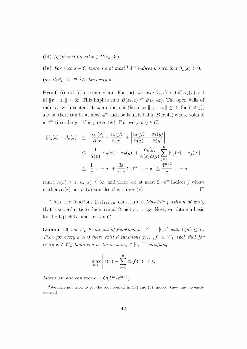
(iii) βk(x) = 0 for all x /∈ B(zk, 3ε).

(iv) For each x ∈ C there are at most34 4m indices k such that βk(x) > 0.

(v) L(βk) ≤ 4m+2/ε for every k.

Proof. (i) and (ii) are immediate. For (iii), we have βk(x) > 0 iff αk(x) > 0

iff ‖x − zk‖ < 3ε. This implies that B(zk, ε) ⊆ B(x, 4ε). The open balls of

radius ε with centers at zk are disjoint (because ‖zk − zj‖ ≥ 2ε for k 6= j),

and so there can be at most 4m such balls included in B(x, 4ε) whose volume

is 4m times larger; this proves (iv). For every x, y ∈ C:

|βk(x) − βk(y)| ≤∣

∣

∣

∣

αk(x)

α(x)− αk(y)

α(x)

∣

∣

∣

∣

+

∣

∣

∣

∣

αk(y)

α(x)− αk(y)

α(y)

∣

∣

∣

∣

≤ 1

α(x)|αk(x) − αk(y)| + αk(y)

α(x)α(y)

K∑

j=1

|αj(x) − αj(y)|

≤ 1

ε‖x − y‖ +

3ε

ε · ε2 · 4m ‖x − y‖ ≤ 4m+2

ε‖x − y‖

(since α(x) ≥ ε, αk(x) ≤ 3ε, and there are at most 2 · 4m indices j where

neither αj(x) nor αj(y) vanish); this proves (v). ¤

Thus, the functions (βk)1≤k≤K constitute a Lipschitz partition of unity

that is subordinate to the maximal 2ε-net z1, ..., zK . Next, we obtain a basis

for the Lipschitz functions on C.

Lemma 16 Let WL be the set of functions w : C → [0, 1] with L(w) ≤ L.

Then for every ε > 0 there exist d functions f1, ..., fd ∈ WL such that for

every w ∈ WL there is a vector ≡ w ∈ [0, 1]d satisfying

maxx∈C

∣

∣

∣

∣

∣

w(x) −d

∑

i=1

ifi(x)

∣

∣

∣

∣

∣

< ε.

Moreover, one can take d = O(Lm/εm+1).

34We have not tried to get the best bounds in (iv) and (v); indeed, they may be easilyreduced.

42

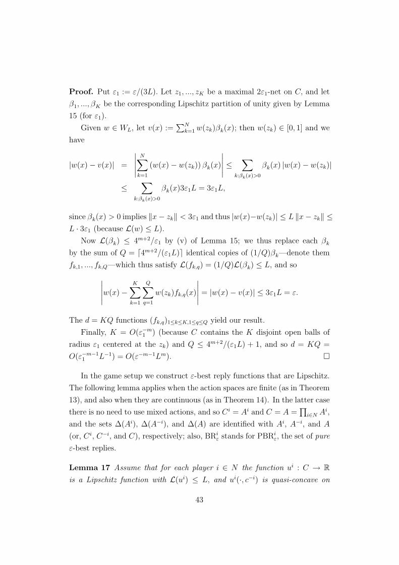
Proof. Put ε1 := ε/(3L). Let z1, ..., zK be a maximal 2ε1-net on C, and let

β1, ..., βK be the corresponding Lipschitz partition of unity given by Lemma

15 (for ε1).

Given w ∈ WL, let v(x) :=∑N

k=1 w(zk)βk(x); then w(zk) ∈ [0, 1] and we

have

|w(x) − v(x)| =

∣

∣

∣

∣

∣

N∑

k=1

(w(x) − w(zk)) βk(x)

∣

∣

∣

∣

∣

≤∑

k:βk(x)>0

βk(x) |w(x) − w(zk)|

≤∑

k:βk(x)>0

βk(x)3ε1L = 3ε1L,

since βk(x) > 0 implies ‖x − zk‖ < 3ε1 and thus |w(x)−w(zk)| ≤ L ‖x − zk‖ ≤L · 3ε1 (because L(w) ≤ L).

Now L(βk) ≤ 4m+2/ε1 by (v) of Lemma 15; we thus replace each βk

by the sum of Q = ⌈4m+2/(ε1L)⌉ identical copies of (1/Q)βk—denote them

fk,1, ..., fk,Q—which thus satisfy L(fk,q) = (1/Q)L(βk) ≤ L, and so

∣

∣

∣

∣

∣

w(x) −K

∑

k=1

Q∑

q=1

w(zk)fk,q(x)

∣

∣

∣

∣

∣

= |w(x) − v(x)| ≤ 3ε1L = ε.

The d = KQ functions (fk,q)1≤k≤K,1≤q≤Q yield our result.

Finally, K = O(ε−m1 ) (because C contains the K disjoint open balls of

radius ε1 centered at the zk) and Q ≤ 4m+2/(ε1L) + 1, and so d = KQ =

O(ε−m−11 L−1) = O(ε−m−1Lm). ¤

In the game setup we construct ε-best reply functions that are Lipschitz.

The following lemma applies when the action spaces are finite (as in Theorem

13), and also when they are continuous (as in Theorem 14). In the latter case

there is no need to use mixed actions, and so Ci = Ai and C = A =∏

i∈N Ai,

and the sets ∆(Ai), ∆(A−i), and ∆(A) are identified with Ai, A−i, and A

(or, Ci, C−i, and C), respectively; also, BRiε stands for PBRi

ε, the set of pure

ε-best replies.

Lemma 17 Assume that for each player i ∈ N the function ui : C → R

is a Lipschitz function with L(ui) ≤ L, and ui(·, c−i) is quasi-concave on

43

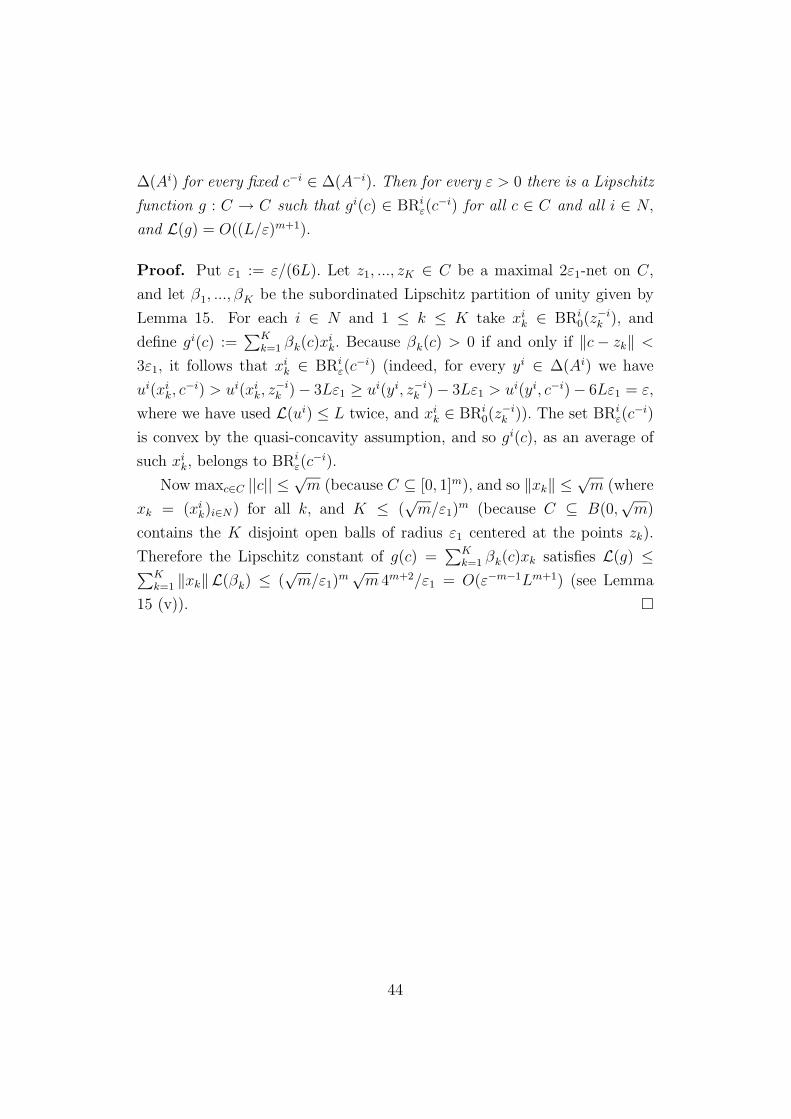
∆(Ai) for every fixed c−i ∈ ∆(A−i). Then for every ε > 0 there is a Lipschitz

function g : C → C such that gi(c) ∈ BRiε(c

−i) for all c ∈ C and all i ∈ N,

and L(g) = O((L/ε)m+1).

Proof. Put ε1 := ε/(6L). Let z1, ..., zK ∈ C be a maximal 2ε1-net on C,

and let β1, ..., βK be the subordinated Lipschitz partition of unity given by

Lemma 15. For each i ∈ N and 1 ≤ k ≤ K take xik ∈ BRi

0(z−ik ), and

define gi(c) :=∑K

k=1 βk(c)xik. Because βk(c) > 0 if and only if ‖c − zk‖ <

3ε1, it follows that xik ∈ BRi

ε(c−i) (indeed, for every yi ∈ ∆(Ai) we have

ui(xik, c

−i) > ui(xik, z

−ik )− 3Lε1 ≥ ui(yi, z−i

k )− 3Lε1 > ui(yi, c−i)− 6Lε1 = ε,

where we have used L(ui) ≤ L twice, and xik ∈ BRi

0(z−ik )). The set BRi

ε(c−i)

is convex by the quasi-concavity assumption, and so gi(c), as an average of

such xik, belongs to BRi

ε(c−i).

Now maxc∈C ||c|| ≤ √m (because C ⊆ [0, 1]m), and so ‖xk‖ ≤ √

m (where

xk = (xik)i∈N) for all k, and K ≤ (

√m/ε1)

m (because C ⊆ B(0,√

m)

contains the K disjoint open balls of radius ε1 centered at the points zk).

Therefore the Lipschitz constant of g(c) =∑K

k=1 βk(c)xk satisfies L(g) ≤∑K

k=1 ‖xk‖L(βk) ≤ (√

m/ε1)m√

m 4m+2/ε1 = O(ε−m−1Lm+1) (see Lemma

15 (v)). ¤

44