serianex teil 393e9dd8c-f2f6-41b7-8c96-ee... · 2014. 4. 30. · induced seismicity ap 3000...
TRANSCRIPT

Induced Seismicity AP 3000
SERIANEX AP 3000
Note
Some data used in this study belongs to Geopower Basel AG. Data and concepts
published in this study may not be further used without written approval of Geopower
Basel AG.

Induced Seismicity AP 3000
SERIANEX AP 3000 - 1/86
AP 3000 Report
Report title: AP3000 Report - Induced Seismicity
Author(s): Stefan Baisch
Robert Vörös
Company: Q-con GmbH Marktstr. 39 76887 Bad Bergzabern Germany
Version: 6
Ref.: KBA001
Report date: 22nd October 2009

Induced Seismicity AP 3000
SERIANEX AP 3000 - 2/86
CONTENTS
1 Overview.............................................................................9
2 Conceptual Model of the Basel Reservoir.....................10
2.1 HYDRAULIC RESERVOIR MODEL .................................................................... 10
2.2 RESERVOIR GEOMETRY ................................................................................ 14
2.2.1 Background...................................................................................................................... 14
2.2.2 Hypocenter Locations ...................................................................................................... 14
2.2.3 Existing Geometrical Models ........................................................................................... 15
2.2.4 Hypothesis Testing: Minimum Complexity Model............................................................ 17
2.3 KAISER EFFECT............................................................................................ 20
2.4 CHARACTERISTICS OF THE LARGEST MAGNITUDE EVENTS............................... 21
2.5 HYDRO-MECHANICAL MODEL ........................................................................ 23
3 Numerical Simulations....................................................24
3.1 STRATEGY ................................................................................................... 24
3.2 MODEL SETUP.............................................................................................. 25
3.3 SIMULATION OF THE DECEMBER 2008 STIMULATION........................................ 26
3.4 CIRCULATION WITHOUT ADDITIONAL STIMULATION........................................... 30
3.5 CIRCULATION AFTER RE-STIMULATING INJECTION WELL ................................... 33
3.6 CIRCULATION AFTER RE-STIMULATING INJECTION & PRODUCTION WELLS .......... 35
3.7 MAXIMUM MAGNITUDE ESTIMATES.................................................................. 36
3.7.1 Reservoir re-stimulation................................................................................................... 36
3.7.2 Circulation ........................................................................................................................ 36
4 Induced Seismicity in EGS Projects ..............................36
4.1 SEISMIC MOMENT VS. INJECTED VOLUME ....................................................... 36
4.2 MAXIMUM MAGNITUDE VS. RESERVOIR SIZE ................................................... 36
4.3 INDUCED SEISMICITY DURING CIRCULATION IN THE SOULTZ RESERVOIR ........... 36
5 Conclusions .....................................................................36
6 References .......................................................................36
7 Appendix 1: Absolute Hypocenter Locations...............36
8 Appendix 2: EGS Parameter Study................................36
8.1 DATA SOURCES ........................................................................................... 36

Induced Seismicity AP 3000
SERIANEX AP 3000 - 3/86
9 Appendix 3: Review and re-evaluation of the hydraulic tests performed in borehole BS-1..................................36
9.1 REVIEW AND RE-EVALUATION OF THE HYDRAULIC TESTS PERFORMED IN BOREHOLE
BS-1............................................................................................................ 36
9.2 THE BOREHOLE BS-1 ................................................................................... 36
9.3 PRE-STIMULATION TESTS .............................................................................. 36
9.3.1 Summary of the pre-stimulation tests .............................................................................. 36
9.4 WATERFRAC-TEST ....................................................................................... 36
9.5 SHUT-IN PERIOD ........................................................................................... 36
9.6 BACK-FLOW-PERIOD .................................................................................... 36
9.7 SUMMARY .................................................................................................... 36
9.7.1 Pre-stimulation tests ........................................................................................................ 36
9.7.2 Stimulation test ................................................................................................................ 36
9.7.3 Post-frac observations ..................................................................................................... 36

Induced Seismicity AP 3000
SERIANEX AP 3000 - 4/86
LIST OF FIGURES
Figure 1: AP3000 workflow.................................................................................................... 9
Figure 2: (Left) Absolute hypocenter locations in map view after Häring et al. (2008).(Right) Relative hypocenter locations in map view after Deichmann and Giardini (2009)..15
Figure 3: Schematic model of reservoir development in an assumed pre-existing cataclastic fracture zone (Figure from Häring et al., 2008)......................................................16
Figure 4: Structural fault model derived in AP2000 (8 faults). ...............................................17
Figure 5: Hypocenter locations (data subset) after collapsing on a 4.2σ confidence level in map view (left) and in side view looking from the East (right). Figure from Asanuma (2006). ..................................................................................................................19
Figure 6: Hypocenter locations after collapsing on a 2σ confidence level (re-processed in the current study) looking from the East (right) and along the dominating planar structure (left). Coordinates are given with respect to the flow exit (611659/270619/4420 m.u.M). ..............................................................................19
Figure 7: Absolute hypocenter locations in perspective view for events occurring prior to shut-in on Dec 8th, 2006 11:30 (left), and for events occurring after shut-in (right). Flow exit is marked in red (right hand panel). Coordinates are given with respect to the flow exit (611659/270619/4420 m.u.M). ..........................................................20
Figure 8: Epicenter map with focal mechanisms for the 28 strongest events. Figure from Deichmann and Ernst (2009). ...............................................................................21
Figure 9: Hypocenter locations of 4 large magnitude events (spheres) in perspective view. Seismic activity that occurred prior to the large magnitude events is indicated by black dots. Note that the largest magnitude events are always located at the outer rim of the region of previous seismic activity. ........................................................22
Figure 10: Temperature drawdown as a function of the separation between injection and production well for a single fracture model. The temperature drawdown is shown after circulating 50 l/s for 30 years. An initial reservoir temperature of 170°C and a re-injection temperature of 90°C have been assumed...........................................25
Figure 11: Observed and modelled wellhead pressures as a function of time (blue). Injection/flow rate is annotated in red. The injection history is divided into 9 different intervals (bottom bar) referred to in subsequent figures. .......................................27
Figure 12: (Top) Moment magnitude of modelled seismicity as a function of time for 20 days. The maximum magnitude event occurred during shut-in (marked by red square). (Bottom) Local magnitude of modelled and observed events as a function of time. Local magnitude of the modelled seismicity has been determined using the formula ML=1.56Mw-1.03 as provided by SED. ..................................................................28
Figure 13: Distribution of hydraulic overpressures inside the fault zone at the time when the largest magnitude event occurred. Grey shading denotes overpressures in MPa according to the grey map. Solid line denotes the location of the injection well. Patches that slipped in the course of the largest magnitude event are marked in black. The largest magnitude event occurred at the outer rim of the previously stimulated region. .................................................................................................29

Induced Seismicity AP 3000
SERIANEX AP 3000 - 5/86
Figure 14: Hydraulic overpressures inside the fault zone as a function of radial distance to the injection well for the time of shut-in (dashed line) and for the time when the largest magnitude event occurred (solid line). The shaded area marks the location of those patches slipping in the course of the largest magnitude event. At these locations, fluid overpressure increased after shut-in..............................................29
Figure 15: Radial distance of seismic events to the injection well plotted against time. Bottom bar indicates the injection history according to Figure 11. .....................................30
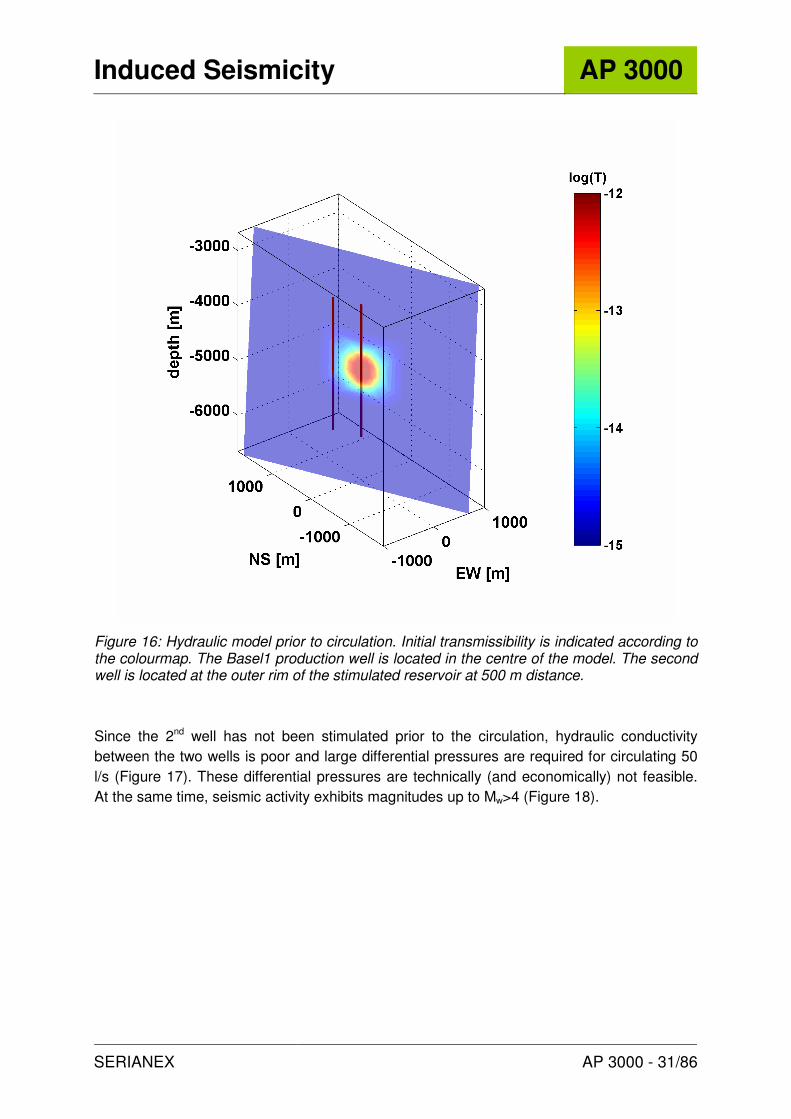
Figure 16: Hydraulic model prior to circulation. Initial transmissibility is indicated according to the colourmap. The Basel1 production well is located in the centre of the model. The second well is located at the outer rim of the stimulated reservoir at 500 m distance. ...............................................................................................................31
Figure 17: Hydraulic pressure at the production well (blue) and the injection well (red) as a function of time during circulation of 50 l/s for 100 days. .......................................32
Figure 18: Magnitude of modelled seismicity as a function of time for a circulation period of 100 days. In this scenario several events with M>4 occurred................................32
Figure 19: Magnitude of modelled seismicity as a function of time for the re-stimulation of the Basel1 well with 60 l/s. Note the Kaiser Effect at an early stage of the re-stimulation. Maximum magnitude is approximately Mw=3.3...................................33
Figure 20: Same as Figure 16 with the Basel1 production well being re-stimulated prior to the circulation. ............................................................................................................34
Figure 21: Magnitude of modelled seismicity as a function of time for a circulation period of 100 days. In this scenario, one event with Mw>4 occurred (indicated by red box)..34
Figure 22: Magnitude of modelled seismicity as a function of time for the stimulation of the production well with 60 l/s. Maximum magnitude is Mw=3.3. .................................35
Figure 23: Same as Figure 16 with both wells being (re-) stimulated prior to the circulation. 36
Figure 24: Magnitude of modelled seismicity as a function of time for a circulation period of 100 days. Maximum event magnitude is Mw=3.1...................................................36
Figure 25: Magnitude-frequency distribution of the modelled seismicity during re-stimulation of the injection well (shown in Figure 19) and stimulation of the production well (shown in Figure 25) over a period of 6 days each. Shaded line indicates data fit with b=1.1. The data fit has been used for estimating a maximum magnitude of Mw=3.7 +/- 0.4 (red circle). ....................................................................................36
Figure 26: Magnitude-frequency distribution of modelled seismicity during the first year of circulating 50 l/s. The blue line indicates a data fit with b=1.7. For comparison, the red line indicates b=1.1 as determined for the stimulation seismicity. Note the lacking of intermediate size events. See text for details. .......................................36
Figure 27: Ratio between the cumulative seismic moment and the cumulative injected volume as a function of time for the injection experiments listed in Table 3. Note that seismic data catalogues are not necessarily complete and the cumulative seismic moment might thus be underestimated (the prominent “kink” at approx. 20 days in the gdy03 data [Cooper Basin, 2003] is caused by a network downtime)..36
Figure 28: Maximum event magnitude (ML) as a function of the logarithm of the reservoir extension A observed during the stimulation of the Cooper Basin reservoir in 2003.
Solid line shows linear fit (with c1=1.4 in (eq 5), dashed lines denote 2σ confidence limits. ....................................................................................................................36

Induced Seismicity AP 3000
SERIANEX AP 3000 - 6/86
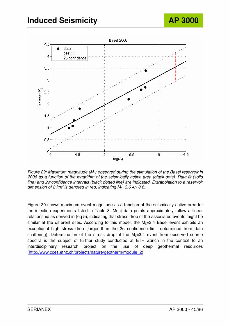
Figure 29: Maximum magnitude (ML) observed during the stimulation of the Basel reservoir in 2006 as a function of the logarithm of the seismically active area (black dots). Data
fit (solid line) and 2σ confidence intervals (black dotted line) are indicated. Extrapolation to a reservoir dimension of 2 km2 is denoted in red, indicating ML=3.6 +/- 0.6. ..................................................................................................................36
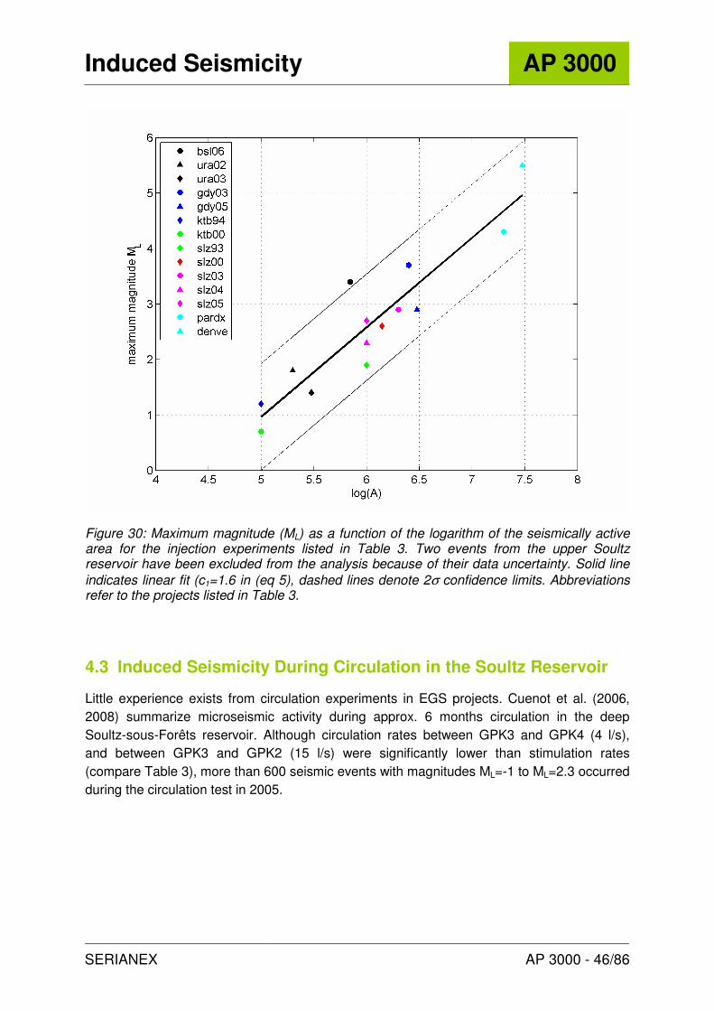
Figure 30: Maximum magnitude (ML) as a function of the logarithm of the seismically active area for the injection experiments listed in Table 3. Two events from the upper Soultz reservoir have been excluded from the analysis because of their data
uncertainty. Solid line indicates linear fit (c1=1.6 in (eq 5), dashed lines denote 2σ confidence limits. Abbreviations refer to the projects listed in Table 3. ..................36
Figure 31: Wadati diagram of a magnitude 2.6 event occurring on December 8th, 2006 03:06:25................................................................................................................36
Figure 32: Histogram of Vp/Vs ratios determined from Wadati diagrams. For compiling Wadati diagrams, only those phase readings have been considered which were used by Geothermal Explorers Ltd. for hypocenter determination. ........................36
Figure 33: (top) Trace normalized, unfiltered waveform section of an M2.2 event occurring on December 8th, 2006 09:04:01. Phase readings used by Geothermal Explorers Ltd. for hypocenter determination are indicated by red/green vertical lines. (bottom) Close up of phase onsets at station Otterbach2 (left) and Riehen (right). Note that phase onsets are not properly assigned................................................................36
Figure 34: Comparison between absolute hypocenter locations determined by Geothermal Explorers (Häring et al., 2008) and determined by Q-con in map view (left) and in perspective view (right). Coordinates are given with respect to the flow exit (611659/270619/4420 m.u.M). ..............................................................................36
Figure 35: Scheme of borehole BS-1 and geologic profile. (Source: Geothermal Explorers) 36
Figure 36: Records of flow rate (top) and wellhead pressure (bottom) of the pre-stimulation tests in borehole BS-1 (source: Ladner & Häring, 2007). ......................................36
Figure 37: Record of the wellhead pressure versus the fourth-root of time of test period 10 (s. Figure 36). (Source: Jung & Ortiz, 2007)...............................................................36
Figure 38: Left: Scheme illustrating bilinear flow. The fluid is leaving the borehole (circle) via an axial fracture. While flowing along the fracture, part of the fluid is permeating into the matrix. Right: Typical pressure field around the fracture for bilinear flow. .36
Figure 39: Top: Log-Log-Plot of the wellhead pressure and of the pressure derivative of test period 10 and fit-curves determined with the well testing program SAPHIR. Bottom: Wellhead pressure record (blue line) and fit curve calculated with the well testing program SAPHIR. Note the discrepancy between record and fit curve when the wellhead pressure exceeded 5000 kPa (5 MPa). (Source: Jung & Ortiz, 2007). ...36
Figure 40: Records of flow (bottom) and wellhead pressure (top) of the waterfrac-test in borehole BS-1. Start of the test was Dezember 1, 2006. The time periods numbered are considered in more detail in the following chapters. (Source: Ladner, F., pers. com.).......................................................................................................36
Figure 41: Record of the wellhead pressure during the starting period (period 1 in Figure 40). The deviation of the recorded pressure from the calculated pressure indicates that fracture stimulation (shearing) started at about 5 MPa. (Source: Ortiz, A., pers. Comm.).................................................................................................................36

Induced Seismicity AP 3000
SERIANEX AP 3000 - 7/86
Figure 42: Transmissibility values calculated for the different flow rate steps of the starting period (period 1 in Figure 36) of the waterfrac-test. (Source: Jung & Ortiz, 2007) .36
Figure 43: Pressure record of the shut-in period following the waterfrac-test. ∆p: friction pressure loss in the fracture, pISI: instantaneous shut-in pressure, p· : initial slope of the pressure decline. The flow rate before shut-in was 0.030 m³/s........................36
Figure 44: Reservoir model used for the evaluation of the pressure decline during the shut-in period. The model consists of a fracture with infinite fracture conductivity and a constant fracture storage coefficient Sf imbedded in a matrix (granite) with permeability k and specific storage coefficient s. The colors of the figure on the right illustrate the pressure field around the fracture. (Source: Ortiz, A., pers. comm.)..................................................................................................................36
Figure 45: Normalized pressure decline during shut-in of the frac-test and type curves for the reservoir model described above. ps= pISI: Instantaneous shut-in pressure (overpressure referred to the formation fluid pressure), p: actual pressure, ts: duration of the frac-test. ........................................................................................36
Figure 46: Record of the water volume produced from borehole BS-1 after the frac-test (top), of the wellhead pressure (bottom, left part) and the pressure measured at 35 m depth (bottom, left part). Note the eruptive production phases starting about 90 days after shut-in. (Data Source: Geothermal Explorers) ......................................36
Figure 47: Plot of the volume produced from borehole BS-1 as a function of the square-root of time. Time zero is the start of venting. (Data source: Geothermal Explorers) ...36
Figure 48: Plots of the fluid level rise in borehole BS-1 after eruption for different eruption periods. The Fluid level is plotted versus a square-root superposition time...........36

Induced Seismicity AP 3000
SERIANEX AP 3000 - 8/86
LIST OF TABLES
Table 1: Hydraulic parameters of the reservoir. ....................................................................13
Table 2: Station dependent seismic velocities obtained by associating early seismicity to the flow exit.................................................................................................................36
Table 3: Key parameters for different injection experiments estimated from published literature. Note: loosely constrained data is given in brackets. Data source column indicates if raw data has been available for the current study. *Aseis is an estimate of the seismically active area determined as the maximum area fitting into the (potentially volumetric) hypocenter distribution. **Magnitude estimates based on the downhole network at Soultz-sous-Forêts might underestimate actual magnitudes by as much as two magnitude units (e.g. compare Jones, 1997 to Baria et al., 1995)..................................................................................................36
Table 4: Range of rock properties determined with the above equations..............................36
Table 5: Range of fracture properties determined with the above equations.........................36
Table 6: Summary of the hydraulic parameters. ...................................................................36

Induced Seismicity AP 3000
SERIANEX AP 3000 - 9/86
1 OVERVIEW
AP3000 is one of seven work packages of the SERIANEX seismic risk analysis for the Basel geothermal system. The focus of AP3000 is on induced seismicity, which comprises seismic events occurring inside the geothermal reservoir. Seismicity that might be triggered further away from the reservoir is addressed in a separate work package (AP4000).
Figure 1 shows the workflow for AP3000. We follow two different lines of investigation; one of them is based on numerical simulations of seismo-hydraulic processes (left hand branch in Figure 1) to estimate the maximum event magnitude and the magnitude-frequency distribution during 30 years of circulation.
The second line of investigation is based on observations made in other EGS projects or during comparable fluid injection experiments, respectively (right hand branch in Figure 1). Empirical relationships between hydraulic parameters and associated seismic activity are used to obtain an estimate for the maximum event magnitude that may occur in the Basel reservoir during stimulation activities.
Figure 1: AP3000 workflow.

Induced Seismicity AP 3000
SERIANEX AP 3000 - 10/86
2 CONCEPTUAL MODEL OF THE BASEL RESERVOIR
2.1 Hydraulic Reservoir Model
A number of hydraulic pre-stimulation tests and a massive waterfrac-test have been performed in borehole BS-1 in October and December 2006 in order to determine the hydraulic properties of the “undisturbed” granite and to create a large fracture system in the granite. The tests were described and analyzed by several groups (Solexperts, Leibniz Institute of Applied Geophysics, and Geothermal Explorer).
As induced seismicity caused serious concerns, no significant post-frac hydraulic tests have been performed. Therefore, the hydraulic properties of the stimulated fracture system can only be determined from observations made during the shut-in and the backflow period following the stimulation test. Due to the limited amount of data (and the general, inherent ambiguity of hydraulic data analysis), no hydraulic reservoir model of the stimulated fracture system at Basel has been determined.
As part of the current study, additional data analysis had to be performed for deriving a reservoir model which is consistent with hydraulic and seismological observations. The guiding questions for the analysis were:
• What are the hydraulic properties of the “undisturbed” granite?
• What are the initial (starting) conditions for the stimulation?
• Is the borehole intersecting (or is located in close proximity to) a permeable fault that might be important for the development of the stimulated fracture system?
• At what pressure level does the “stimulation” start and how is the pressure developing during stimulation?
• What are the hydraulic properties of the fracture or fracture system created or activated during the waterfrac-test?
• Is the created or activated fracture or fracture system hydraulically connected to a major fault at some distance to the borehole?
The data analysis is described in section 9 (Appendix 3). The results can be summarized as follows:
The analysis of pre-stimulation hydraulic tests revealed that the hydraulic response of the (400 m) openhole section in the granite is most likely dominated by an axial fracture. The results are consistent with a fracture of limited height in a narrow fault zone of moderate permeability, or alternatively, with a fracture with larger height in competent granite. Due to this ambiguity it is not possible to determine a single permeability value for the granite. Considerations based on a bilinear flow model, however, revealed a permeability value in the

Induced Seismicity AP 3000
SERIANEX AP 3000 - 11/86
order of 1 to 10 micro-Darcy. For both models, the area of investigation is about 2000 m² to 10000 m² corresponding to either the fault area (model 1) or the fracture area (model 2). Both models require the existence of a planar structure (with relatively large area) prior to stimulation activities. The hydraulic conductivity (i.e. transmissibility of the fault, or fracture conductivity) of this structure, however, is comparably low (in the range between 10-15 and 10-14 m³). The hydraulic formation pressure in the granite creates an artesian wellhead pressure of 1.5 MPa to 2 MPa when the borehole is filled with water and is in thermal equilibrium with the surrounding rock formations.
There is no indication for a constant pressure or a “no-flow boundary” within the area of investigation.
During stimulation, the injectivity index of the borehole increased dramatically. Assuming that flow occurred predominantly into a pre-existing fracture, the hydraulic conductivity of this fracture increased by about three orders of magnitude and reached 10-12 m³ at the end of the test. The post-stimulation conductivity was derived from the instantaneous pressure drop after shut-in. Since this pressure drop is a rapid process, the data does not reveal information on the inflow conditions from the well into the fracture and it is not possible to better constrain the fracture conductivity. A fair assumption is that the post-frac fracture conductivity is in the range of 1·10-12 m³ to 1·10-11 m³. The fracture conductivity did not decrease significantly during pressure decline (Jung & Ortiz, 1987).
The record of the injection pressure showed that the increase in fracture conductivity started at a wellhead pressure of about 5 MPa. The irregular trend of the injection pressure during the test clearly indicates that shearing was the dominant stimulation mechanism. Pressure stabilized only during high flow rates at the end of the test indicating that the elastic response of the fracture became more significant. The pressure observed after the instantaneous pressure drop at shut-in is 26.4 MPa above hydrostatic. This pressure can be regarded as a lower bound for the jacking pressure (pressure in balance with the effective normal stress acting on its surface).
Although no significant hydraulic test could be performed after the stimulation test, valuable information could be derived from the pressure decline during shut-in and backflow. The pressure decline observed during the shut-in period could be simulated by using a simple model consisting of a large single fracture with high storage capacitance and high transmissibility, which is loosing fluid into the surrounding homogenous matrix (granite). Using the fracture size determined from the microseismic cloud, the fracture compliance and the permeability of the granite surrounding the fracture (or fault) was determined. With a similar model, the record of the fluid volume during the backflow period could be evaluated. The fracture storage capacitance obtained from these data is approximately 50 m³/MPa for the shut-in period, and approximately 80 m³/MPa for the backflow period. This implies that 50 m³ or 80 m³ of fluid have to flow from the granite into the fracture in order to increase the pressure within the fracture by 1 MPa. The difference between the two values may be attributed to the fact that fracture size increased significantly during the shut-in and the early part of the backflow period.
Induced Seismicity AP 3000
SERIANEX AP 3000 - 12/86
The fracture storage capacitance can be used to determine the large scale fracture compliance (elastic change of fracture width). Assuming that the fracture size is identical to the area defined by the micro-seismic events we obtain 8· 10-11 m³/Pa for both cases.
The large scale permeability value for the granite derived from the shut-in period is 3·10-18 m2. For the backflow period, however, we obtain a value of only 3·10-20 m2. This discrepancy might reflect that the fracture continued to propagate during shut-in. The fluid volume consumed by this process accelerates the pressure decline thus pretending a higher permeability of the rock. The permeability estimate of 3·10-18 m2 is therefore an upper limit for the large scale permeability of the granite. On the other hand, the artesian pressure of 2 MPa assumed for the evaluation of the back-flow period might be overestimated. A value of 1 MPa, for example, would result in a permeability value close to 1·10-19 m². Since it is unlikely that the artesian pressure under the prevailing conditions is significantly lower than 1 MPa, it is almost certain that the large scale permeability of the granite is substantially smaller than 1 Micro-Darcy and most likely even smaller than 0.1 Micro-Darcy. It should be mentioned that the permeability would be even smaller when the “hydraulic” fracture size is larger than the seismically active fracture area. An assumption that is not unreasonable.
Fluid balance considerations based on the results on a permeability value of 1·10-19 m² show that during the stimulation test the majority of the injected fluid (about 80 %) was used for creating new fracture volume and that a much smaller part permeated into the matrix (granite). The hydraulic parameter values determined by this study are listed in Table 1.
Of primary importance for the current study is the question whether or not the fracture (in its current state) might be connected to a larger scale hydraulic feature (e.g. major fault). Within the radius of investigation (approximately 1500 m) there is no indication for a constant pressure boundary and a connection to a highly conductive larger scale feature can almost certainly be excluded.
Another important question concerning the triggering of post-injection seismicity is, to what extend the reservoir has been over-pressurized in the post-injection period. It had been suspected that the eruptive overflow of the borehole persisting until today might be driven by the relict of the overpressure created during stimulation. Unfortunately, no long term pressure build-up recordings exist for the post-stimulation period and information on hydraulic overpressures can only be obtained indirectly from outflow recordings. Analysis of this data indicates that the overpressure in the bulk of the reservoir might not be higher than the artesian pressure. However, since stimulation is a non-reversible process, it can not be excluded that in parts of the reservoir the pressure decline took much longer than the pressure build-up and that overpressures resulting from the stimulation may persist for a significantly longer period of time. In this case, hydraulic overpressures might also be responsible for the post-injection seismicity observed at the outer rim of the stimulated area.

Induced Seismicity AP 3000
SERIANEX AP 3000 - 13/86
Parameter Unit Range
possible
Range
likely
Large scale permeability of the granite m² 3·10-20 - 1·10-17 3·10-20 - 1·10-19
Storage coefficient of the granite (assumed)
1/Pa 1·10-11 - 1·10-10 1·10-11
Pre-frac artesian pressure MPa 1.5 – 2.5 1.5 – 2
Post-frac artesian pressure MPa 0.2 – 2.5 1 – 2
Pre-frac fracture conductivity m³ 1·10-13 – 3·10-16 1·10-14 – 1·10-15
Pre-frac fault transmissibility m³ 1·10-16 – 1·10-15 1·10-15
Post-frac fracture conductivity m³ 1·10-12 - 1·10-11 1·10-12
Fracture compliance (elastic response) m/Pa 5·10-11 - 1·10-10 8·10-11
Fracture compliance simulating fracture opening during stimulation
m/Pa 5·10-10 -1·10-9 5·10-10 -1·10-9
wellhead pressure for the onset of shearing
MPa 5 5
wellhead jacking pressure MPa ≥ 26.4 ≥ 26.4
Table 1: Hydraulic parameters of the reservoir.

Induced Seismicity AP 3000
SERIANEX AP 3000 - 14/86
2.2 Reservoir Geometry
2.2.1 Background
The maximum magnitude of a seismic event that may occur in a geothermal reservoir is critically depending on the reservoir geometry. In general, the strength (or magnitude) of an earthquake is controlled by the size of the associated shearing plane and the amount of shear slip occurring on the plane.
Simple mechanical considerations reveal that the shear slip cannot become arbitrary large, but is limited by (i) the capacity of the surrounding rock to take up deformation, and (ii) by the amount of shear stress driving the failure process. Therefore, the dominating parameter controlling the magnitude of reservoir events is the area of the associated shearing plane.
The maximum extension of connected shearing planes that may fail in the course of a single earthquake is limited by the reservoir size and the internal fracture complexity (“reservoir geometry”). In the EGS context, the reservoir geometry is commonly determined from the distribution of the induced seismicity. Thereby the “geothermal reservoir” is defined by those regions, where fluid pressure elevation (e.g. during hydraulic stimulations) is sufficient to cause seismic activity.
2.2.2 Hypocenter Locations
Hypocenter locations of the seismicity induced by the Basel 1 stimulation have been determined by different groups:
• Geothermal Explorers Ltd. provides absolute hypocenter locations (Dyer et al., 2008; Häring et al., 2008) using a local seismic velocity model calibrated by events occurring close to the injection well (for details we refer to Schanz et al., 2007). Recordings of 4 downhole instruments have been used for the hypocenter determination. A major drawback of this dataset is the lack of proper confidence estimates for the hypocenter solutions which are stated in terms of RMS (root mean square) values only (i.e. by the misfit in the data space).
• SED (Schweizer Erdbeben Dienst) has determined relative hypocenter locations for the larger magnitude events (i.e. M ≥ 0.7) using a regional seismic velocity model (Deichmann and Giardini, 2009). Besides downhole data, recordings from the SED surface station network have been used for the hypocenter determination.
• For a subset of 2,702 events, Tohoku University has determined absolute hypocenter locations and different types of relative and collapsed hypocenter locations (Asanuma, 2006). Using the phase readings provided by Geothermal Explorers Ltd., these authors were able to reproduce the absolute hypocenter locations of Geothermal Explorers Ltd.
Induced Seismicity AP 3000
SERIANEX AP 3000 - 15/86
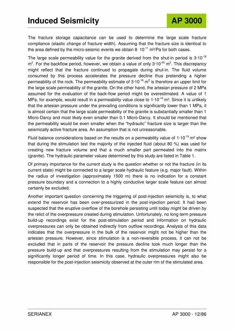
Figure 2: (Left) Absolute hypocenter locations in map view after Häring et al. (2008).(Right) Relative hypocenter locations in map view after Deichmann and Giardini (2009).
2.2.3 Existing Geometrical Models
Hypocenter distributions as determined by the groups listed above consistently indicate one or several subvertical structures of limited width (see Figure 2). These have been interpreted in different ways:
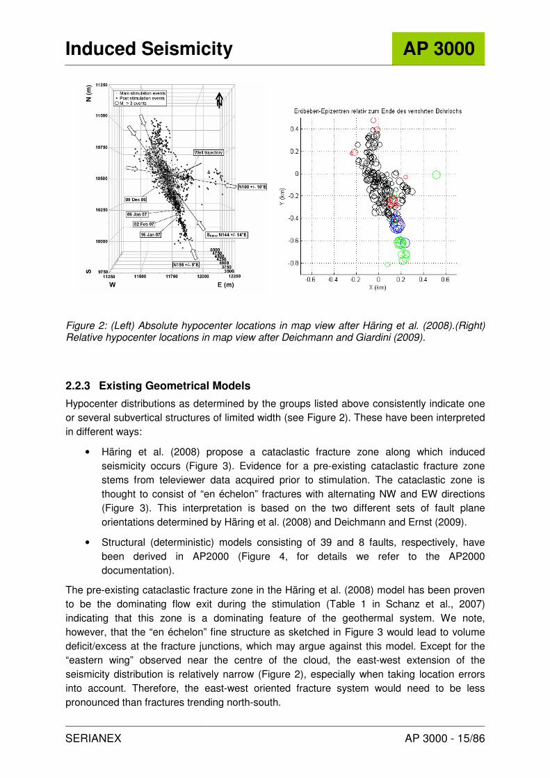
• Häring et al. (2008) propose a cataclastic fracture zone along which induced seismicity occurs (Figure 3). Evidence for a pre-existing cataclastic fracture zone stems from televiewer data acquired prior to stimulation. The cataclastic zone is thought to consist of “en échelon” fractures with alternating NW and EW directions (Figure 3). This interpretation is based on the two different sets of fault plane orientations determined by Häring et al. (2008) and Deichmann and Ernst (2009).
• Structural (deterministic) models consisting of 39 and 8 faults, respectively, have been derived in AP2000 (Figure 4, for details we refer to the AP2000 documentation).
The pre-existing cataclastic fracture zone in the Häring et al. (2008) model has been proven to be the dominating flow exit during the stimulation (Table 1 in Schanz et al., 2007) indicating that this zone is a dominating feature of the geothermal system. We note, however, that the “en échelon” fine structure as sketched in Figure 3 would lead to volume deficit/excess at the fracture junctions, which may argue against this model. Except for the “eastern wing” observed near the centre of the cloud, the east-west extension of the seismicity distribution is relatively narrow (Figure 2), especially when taking location errors into account. Therefore, the east-west oriented fracture system would need to be less pronounced than fractures trending north-south.
Induced Seismicity AP 3000
SERIANEX AP 3000 - 16/86
Figure 3: Schematic model of reservoir development in an assumed pre-existing cataclastic fracture zone (Figure from Häring et al., 2008).

Induced Seismicity AP 3000
SERIANEX AP 3000 - 17/86
Figure 4: Structural fault model derived in AP2000 (8 faults).
2.2.4 Hypothesis Testing: Minimum Complexity Model
One limitation of the geometrical models discussed in the previous section is that hypocenter location errors have not been taken into account. Especially into East-West direction, the true width of the structure is of primary importance for a conceptual model.
A common technique for enhancing structures in hypocenter clouds is the collapsing method (Jones and Stewart, 1997) which implies moving hypocenter locations inside their error ellipsoids towards a common centre of mass. In theory, the distribution of the movement vectors after collapsing – if hypocenters have been moved to their true locations - should
follow a χ2−distribution with three degrees of freedom, assuming that spatial location errors
are normally distributed. Therefore, the χ2−distribution may serve as a ‘a posteriori’
justification that hypocenters have actually been moved to their true locations by the
collapsing process. However, the χ2−distribution fit fails in most cases even for synthetic data
(also for the original data example presented by Jones and Stewart, 1997). Synthetic data

Induced Seismicity AP 3000
SERIANEX AP 3000 - 18/86
tests nevertheless indicate that the collapsing method has the potential to recover true
structures in blurred hypocentral clouds even when the “χ2−criterion” is not fulfilled.
In the current analysis we use the collapsing method for hypothesis testing only. The hypothesis under consideration is whether or not a geometrical model with minimum complexity, i.e. a planar structure, is consistent with the observed data.
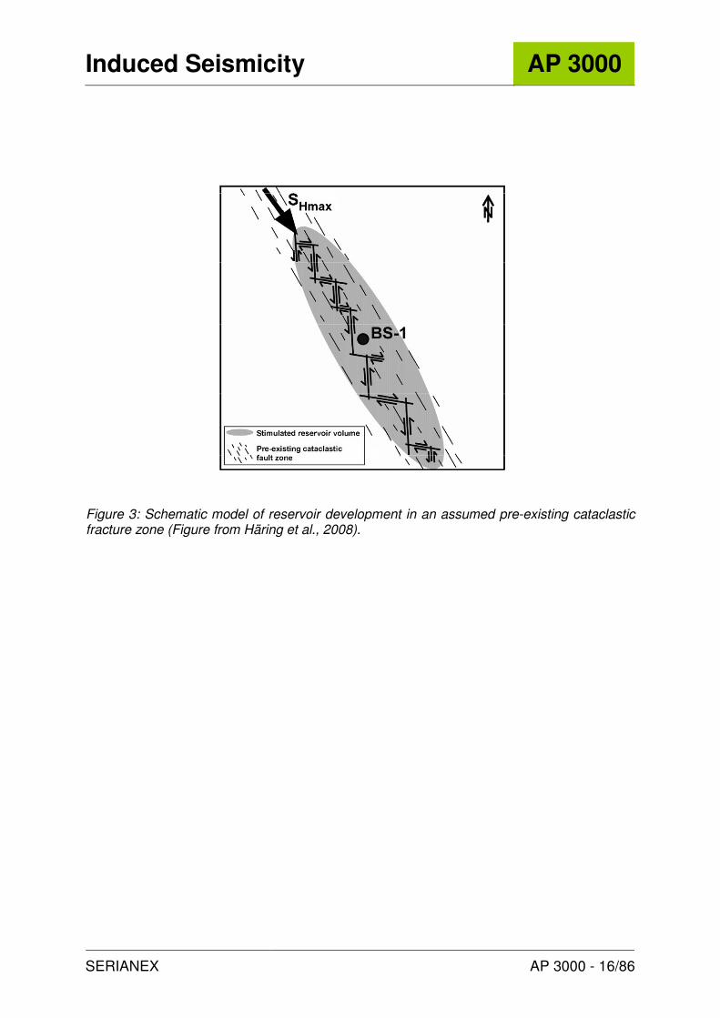
Asanuma (2006) applied the collapsing technique to a data subset and obtained a focussed structure consisting of several streaks (Figure 5). The East-West width of the structure, however, cannot be determined from the display used by Asanuma (collapsed data in digital form was not available for the current study).
To further analyse collapsed hypocenter locations, we have reprocessed the complete
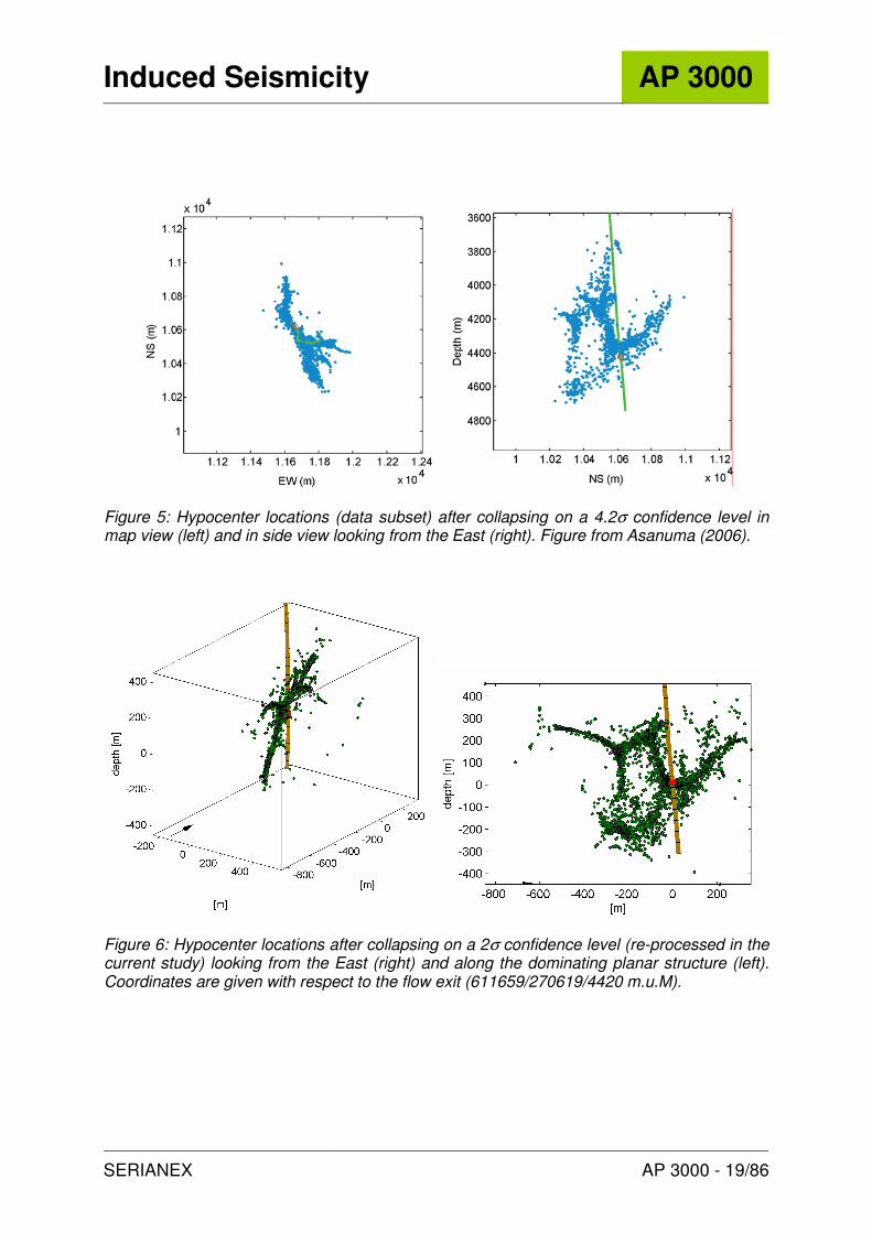
seismic data set (see appendix in section 7) and applied the collapsing method using 2σ confidence ellipsoids. Figure 6 displays the resulting hypocenter distribution. The resulting structure is similar to the one obtained by Asanuma (2006) for a data subset (compare right hand panels in Figure 5 and Figure 6). The distribution is dominated by a curved, planar structure (Figure 6, left) trending NW-SW with a smaller wing into the eastern direction.
Therefore we conclude that the observation data (i.e. hypocenter locations and confidence limits) is consistent with a scenario where most hypocenters are located along a single, planar structure. This implies that minimum complexity models need to be considered where the maximum shearing area is not limited by structural heterogeneity. We note, however, that the impact of such a conservative model assumption (conservative in the sense that maximum magnitudes might be overestimated) on the maximum magnitude estimate is small. Numerical modelling based on the minimum complexity model (section 3) yields maximum earthquake magnitudes1 of Mw=3.7 +/- 0.4. This estimate is in the same order of magnitude that has actually been observed (ML=3.4 corresponding to Mw=3.1).
1 In the context of seismic hazard, the moment magnitude Mw is used instead of the local magnitude ML. In this study, the strength of seismic events will therefore by quantified by Mw whenever possible. Note that for the magnitude range considered here, Mw is slightly smaller than ML.
Induced Seismicity AP 3000
SERIANEX AP 3000 - 19/86
Figure 5: Hypocenter locations (data subset) after collapsing on a 4.2σ confidence level in map view (left) and in side view looking from the East (right). Figure from Asanuma (2006).
Figure 6: Hypocenter locations after collapsing on a 2σ confidence level (re-processed in the current study) looking from the East (right) and along the dominating planar structure (left). Coordinates are given with respect to the flow exit (611659/270619/4420 m.u.M).

Induced Seismicity AP 3000
SERIANEX AP 3000 - 20/86
2.3 Kaiser Effect
Figure 7 compares hypocenter locations of events occurring during the stimulation to hypocenter locations of events occurring post-stimulation. The two distributions are nearly complementary. The region of seismic activity during stimulation remains seismically quiet in the post-stimulation period (except for a few scattered events which might be due to hypocenter location errors).
Similar observations have been made during other fluid injection experiments (Baisch et al., 2002; 2006; 2009; 2009b) and have been interpreted as an expression of the Kaiser Effect (Baisch and Harjes, 2003). In this interpretation, seismicity is induced only at those locations where previously experienced (maximum) fluid overpressures are exceeded. If hydraulic overpressures are controlled by fluid pressure diffusion, then post-injection fluid pressure increase occurs only near the outer boundary of the stimulated reservoir. It should be noted that the characteristic “gap” observed in the centre of the post-injection seismicity distribution (Figure 7, right) is another indicator for the dynamic processes occurring along a planar structure. No such “gap” would have appeared if dynamic processes had induced seismic activity into the normal direction of the plane (i.e. into East-West direction). In that case, the “gap” would have been hidden in the perspective view of Figure 7 (right).
Figure 7: Absolute hypocenter locations in perspective view for events occurring prior to shut-in on Dec 8th, 2006 11:30 (left), and for events occurring after shut-in (right). Flow exit is marked in red (right hand panel). Coordinates are given with respect to the flow exit (611659/270619/4420 m.u.M).

Induced Seismicity AP 3000
SERIANEX AP 3000 - 21/86
2.4 Characteristics of the Largest Magnitude Events
Fault plane solutions have been determined by Deichmann and Ernst (2009) for 28 of the largest magnitude events. Most events exhibit typical strike-slip mechanisms with NS and EW striking nodal planes (Figure 8) which is in agreement with the local stress field around the Basel 1 well. This indicates that the reservoir induced seismicity is driven by the local stress field (Deichmann & Ernst, 2009).
We note, however, that the overall orientation of the seismic cloud (e.g. Figure 2) does not coincide with most of the focal plane orientations shown in Figure 8. In light of the minimum complexity model discussed in section 2.2.4, such a coincidence would be expected if seismic activity had occurred along a single, planar structure, driven by the same stress field. Currently, we do not have an explanation for the observed discrepancy.
Figure 9 compares the hypocenter locations of 4 large magnitude events to the location of the seismic activity occurring prior to the associated large magnitude events. We note that the large magnitude events always occur at the outer rim of the zone of previous seismic activity (we have confirmed this for all events with ML>2.2). The examples shown in Figure 9 have been chosen such that the effect is demonstrated for different positions at the outer rim.
Figure 8: Epicenter map with focal mechanisms for the 28 strongest events. Figure from Deichmann and Ernst (2009).

Induced Seismicity AP 3000
SERIANEX AP 3000 - 22/86
Figure 9: Hypocenter locations of 4 large magnitude events (spheres) in perspective view. Seismic activity that occurred prior to the large magnitude events is indicated by black dots. Note that the largest magnitude events are always located at the outer rim of the region of previous seismic activity.

Induced Seismicity AP 3000
SERIANEX AP 3000 - 23/86
2.5 Hydro-Mechanical Model
Observations discussed in the previous sections indicate that the seismically active region is dominated by one or several subvertical, planar structures. The existence of a larger scale structure is also supported by the fact that an Mw=3.0 event has occurred in the reservoir, which typically requires a shearing plane in the order of several 10,000 m2. Although the seismicity distribution (Figure 2) exhibits an additional wing towards the East (on which no event above magnitude 1.8 occurred), we nevertheless approximate the reservoir geometry by the simplest geometrical model of a single, subvertical plane.
Borehole imaging data obtained prior to the stimulation resolve a cataclastic fracture zone at 4,420 m depth where the near-well seismicity is concentrated. During stimulation, this zone coincides with a prominent flow exit during stimulation, indicating that the reservoir is dominated by a pre-existing fault zone.
The hydraulic response of the reservoir during stimulation does not exhibit pressure-limiting behaviour, indicating that the jacking pressure has not been exceeded (Häring et al., 2008). Below the jacking pressure, the mechanisms causing induced seismicity can be explained by hydraulic overpressures reducing the effective normal stress on existing fractures (Healy et
al. 1970). Let τ and σn denote the shear and normal stresses resolved on a fracture plane, Pfl
the in situ fluid pressure, and µ the coefficient of friction, then slip occurs on the fracture if
(eq 1) τ/(σn−Pfl) > µ
Following Baisch et al. (2009b), we assume that the large-scale fault consists of many smaller fault patches which may slip independently, but are mechanically coupled to their neighbors (so called “block-spring model”, e.g. Bak & Tang, 1989). Slip occurs whenever the resolved shear stress on a patch exceeds the frictional strength. Thereby the shear stress
resolved on the patch is reduced by the amount of stress drop ∆σ and shear stress on the neighbouring patches is increased due to mechanical coupling. Here we assume the same stress transfer pattern as in Baisch et al. (2009b).
Due to stress redistribution, slip on an individual patch may cause overcritical stress conditions on neighbouring patches, thus triggering an “avalanche” of simultaneous slip events. Following previous considerations (section 2.2.1), the number of patches slipping simultaneously (i.e. the shearing area) controls the event magnitude.

Induced Seismicity AP 3000
SERIANEX AP 3000 - 24/86
3 NUMERICAL SIMULATIONS
3.1 Strategy
Based on the conceptual model derived in the previous section, we simulate induced seismicity for different stimulation and circulation scenarios.
Our starting point is the seismic activity observed during the stimulation of the Basel reservoir in 2006. In section 3.3 we use observations from the 2006 stimulation to “calibrate” first order parameters of the numerical model.
The stimulation in 2006 has been aborted early and the current reservoir extension is not sufficient to be economically viable (according to the guidelines presented by Baria & Petty, 2008). Therefore, re-stimulation scenarios are considered in the numerical simulations in sections 3.5 and 3.6.
Additionally, the position of a second wellbore required for the circulation is not determined at this stage. Within the conceptual model derived here (i.e. single fracture model), a comparatively large separation between injection and production well might be required to ensure a sufficient thermal lifetime of the system (say 1 km wellspacing or more, compare Figure 10). However, with the transmissibility determined for the stimulated reservoir (compare section 2.1), a well separation of 1 km would require tremendous differential pressures for the circulation. Therefore we set the well separation to 500 m in our numerical models. Although this value is somewhat arbitrarily chosen (and not based on a proper economic feasibility analysis which would be beyond the scope of the current study), we note that well separations in similar projects (Cooper Basin: 568 m; Soultz: 665 m) are of the same order. We note also, that even for 500 m well spacing, differential pressures of 0.7 MPa/l/s are required in our numerical models when circulating 50 l/s. This value is already beyond the limit of what is considered to be economically feasible by Baria & Petty (2008).

Induced Seismicity AP 3000
SERIANEX AP 3000 - 25/86
Figure 10: Temperature drawdown as a function of the separation between injection and production well for a single fracture model. The temperature drawdown is shown after circulating 50 l/s for 30 years. An initial reservoir temperature of 170°C and a re-injection temperature of 90°C have been assumed.
3.2 Model Setup
We implemented the conceptual model discussed in section 2.5 into a numerical finite-element model. The numerical model consists of a subvertical, rectangular structure, representing a fault zone, which is intersected by a well at a depth of 4,670 m. The fault zone extends over 4,000 m in both, lateral and vertical direction. Effectively, dynamic processes on the fault are not limited by structural boundaries during the simulation runs. To avoid boundary effects for pressure diffusion, the hydraulic model is augmented at the outer rim of the fault zone to a total extension of 20,000 m into horizontal, and 7,000 m into vertical direction. Constant pressure boundaries are implemented in the lateral direction and no-flow boundaries in the vertical direction. The stress field is adopted from Häring et. al. (2008) with maximum and minimum stresses being horizontally oriented and SH striking at N144° +/- 14°.
After initial simulation runs we assume a coefficient of friction of µ=0.64, which is in the range of the frictional limit considered by Häring et al. (2008). The coefficient of friction is a critical parameter determining the productivity of the induced seismicity in the numerical models. With increasing µ, the productivity decreases since criticality on the fracture patches gets lower. The assumed coefficient of friction has been found by approximately matching the modelled productivity with observation data (i.e. observed number of events). We note that µ = 0.64 corresponds to an optimum shearing angle of 29° (with respect to SH). Given the orientation of SH as stated above, the optimum orientation for shear is 173° +/- 14°. The mean orientation of the seismicity distribution (obtained by fitting a plane to the entire seismic cloud) is N158°, which is approximately within the range of optimally oriented faults. It should

Induced Seismicity AP 3000
SERIANEX AP 3000 - 26/86
be noted that uncertainties of the fault zone orientation within the (tectonic) stress field can be translated into uncertainties of the coefficient of friction. The coefficient of friction has been varied in order to match observation data (see above). By this calibration procedure the impact of the uncertainties of the assumed fault zone orientation on the modelling results is minimized.
Based on stress estimates by Häring et al. (2008), the shear stresses resolved prior to
stimulation on our model fault near the injection point are τ = 30.5 MPa. The latter value has been determined by assuming SH=160 MPa which is the lower limit value of Häring et al. (2008). However, the impact of this assumption on the simulation results in section 3 is negligible as long as shear stresses resolved on the fault remain in the same order of magnitude.
We have divided our model fault into quadratic patches of 20 m side length. We assume that slipping of a patch causes an increase of the permeability for the associated patch, thus leading to spatio-temporal changes of the hydraulic parameters. At each time step, the parameter distribution is updated according to our mechanical model and the fluid pressure for the next time sample is computed with respect to the updated distribution. We assume a local permeability enhancement of 25% for each slip and limit the maximum possible enhancement to be 400 fold. With these assumptions we have scaled our model parameters with observed data (compare section 2.1).
Seismic moment is determined from the slipping area (defined by the number of patches
slipping simultaneously) and an assumed (constant) stress drop of ∆σ = 3 MPa. The latter value was determined during the initial simulation runs by approximately matching the maximum magnitude which is most sensitive to the assumed stress drop. Moment magnitudes have been determined using the empirical relationship of Bungum et al. (1982).
3.3 Simulation of the December 2008 stimulation
Figure 11 compares modelled to observed wellhead pressures for the Basel1 stimulation. Modelled peak pressures are in reasonably good agreement with observation data. We notice, however, that the simulated pressure decay in the post-injection period is slower than the observed pressure decay. This difference might be caused by the simplifying model assumption of the rock matrix being hydraulically impermeable. Small leak-off into the matrix, as discussed in section 2.1, could accelerate the pressure decay. Simulating this effect, however, was not possible within the time budget of the current study.
Concerning induced seismicity, the slower (modelled) pressure decay in the post-injection period leads to prolonged seismic activity (as long as overpressures are sufficient to exceed fracture criticality). Therefore, the modelled seismicity tends to overestimate the seismic activity in the post-injection period.

Induced Seismicity AP 3000
SERIANEX AP 3000 - 27/86
Figure 11: Observed and modelled wellhead pressures as a function of time (blue). Injection/flow rate is annotated in red. The injection history is divided into 9 different intervals (bottom bar) referred to in subsequent figures.
Figure 12 shows modelled event magnitudes as a function of time. Consistent with observations (Figure 12, bottom; see also section 2.4), the largest magnitude event occurred post-injection and exhibits a magnitude of Mw=2.8. We also note that modelled seismic activity continues throughout the entire time period of 100 days. Different to observed data, modelled seismicity only consists of the smallest and comparatively large magnitude events after approx. 20 days. This can be explained by the underlying homogeneous fault model without structural heterogeneity (prior to stimulation), e.g. with no variations of the fracture orientation, the stress field, or the coefficient of friction. Due to this assumption, fracture criticality in the post-injection period is usually exceeded approximately simultaneously on many neighbouring patches (because of the small spatial fluid pressure gradients in the post-injection period). Structural complexity introduced into the numerical models would modify the magnitude frequency distribution accordingly. In general, the impact of structural heterogeneities becomes more important when the magnitude of hydraulic overpressures is small and in the same range as the stress heterogeneities. This effect occurs predominantly at a late stage of the numerical simulations.
It should also be noted that the modelled seismic activity extends into all directions along the fault. Observed data (e.g. Figure 6 and Figure 7) indicate that the hypocenter distribution may not be symmetric. If structural variations limit the spatial extension of the seismic activity, then the modelled catalogue overestimates actual seismicity. By comparing the number of modelled Mw≥2 events (32 events) to the number of Mw≥2 events observed during the stimulation period (10 events), we obtain an overestimation factor of approximately 3.

Induced Seismicity AP 3000
SERIANEX AP 3000 - 28/86
Figure 12: (Top) Moment magnitude of modelled seismicity as a function of time for 20 days. The maximum magnitude event occurred during shut-in (marked by red square). (Bottom) Local magnitude of modelled and observed events as a function of time. Local magnitude of the modelled seismicity has been determined using the formula ML=1.56Mw-1.03 as provided by SED.
Figure 13 shows the location of the patches that slipped in the course of the largest magnitude event. Consistent with observations (Figure 9, bottom left), the modelled event occurred at the outer rim of the previously stimulated reservoir (however, the modelled event occurred at the upper reservoir boundary, whereas the actual event occurred at the lower reservoir boundary). At this location, fluid overpressures keep increasing after shut-in, exhibiting relatively shallow spatial gradients (Figure 14). Therefore, many neighbouring patches are on a similar level of stress criticality, thus increasing the likelihood for the occurrence of slip avalanches (i.e. large magnitude events). In this scenario, only a small amount of stress-diffusion is sufficient to cause overcritical conditions over a larger area.

Induced Seismicity AP 3000
SERIANEX AP 3000 - 29/86
Figure 13: Distribution of hydraulic overpressures inside the fault zone at the time when the largest magnitude event occurred. Grey shading denotes overpressures in MPa according to the grey map. Solid line denotes the location of the injection well. Patches that slipped in the course of the largest magnitude event are marked in black. The largest magnitude event occurred at the outer rim of the previously stimulated region.
Figure 14: Hydraulic overpressures inside the fault zone as a function of radial distance to the injection well for the time of shut-in (dashed line) and for the time when the largest magnitude event occurred (solid line). The shaded area marks the location of those patches slipping in the course of the largest magnitude event. At these locations, fluid overpressure increased after shut-in.

Induced Seismicity AP 3000
SERIANEX AP 3000 - 30/86
The spatio-temporal evolution of the modelled seismicity is shown in Figure 15. Seismic activity systematically migrates away from the injection well with increasing time. The region near the injection well starts getting seismically quiet after approximately 1 day and near-well seismicity occurs only when the injection rate (and thus the injection pressure) is increased. Consistent with observations (section 2.3), post-injection seismicity solely occurs at the outer rim of the zone of previous seismic activity (Kaiser Effect).
Figure 15: Radial distance of seismic events to the injection well plotted against time. Bottom bar indicates the injection history according to Figure 11.
3.4 Circulation without additional stimulation
Based on the numerical model developed in the previous section, we have simulated different scenarios for the geothermal system.
In the first model, a second wellbore has been introduced at 500 m inter-well separation to the existing Basel1 well (Figure 16). No additional stimulations have been performed and the Basel1 well has been assumed to be the production well while circulating at 50 l/s.
Induced Seismicity AP 3000
SERIANEX AP 3000 - 31/86
Figure 16: Hydraulic model prior to circulation. Initial transmissibility is indicated according to the colourmap. The Basel1 production well is located in the centre of the model. The second well is located at the outer rim of the stimulated reservoir at 500 m distance.
Since the 2nd well has not been stimulated prior to the circulation, hydraulic conductivity between the two wells is poor and large differential pressures are required for circulating 50 l/s (Figure 17). These differential pressures are technically (and economically) not feasible. At the same time, seismic activity exhibits magnitudes up to Mw>4 (Figure 18).

Induced Seismicity AP 3000
SERIANEX AP 3000 - 32/86
Figure 17: Hydraulic pressure at the production well (blue) and the injection well (red) as a function of time during circulation of 50 l/s for 100 days.
Figure 18: Magnitude of modelled seismicity as a function of time for a circulation period of 100 days. In this scenario several events with M>4 occurred.

Induced Seismicity AP 3000
SERIANEX AP 3000 - 33/86
3.5 Circulation after re-stimulating injection well
This model is identical to the previous model except that the Basel1 production well has been re-stimulated prior to the circulation. Figure 19 shows modelled seismicity during 6 days re-stimulation at 60 l/s. The reservoir has been depressurized before re-stimulating (i.e. assuming hydrostatic conditions). Therefore, seismicity sets in only after 2.2 days (Kaiser Effect) and exhibits a maximum magnitude of approximately Mw=3.3.
Figure 19: Magnitude of modelled seismicity as a function of time for the re-stimulation of the Basel1 well with 60 l/s. Note the Kaiser Effect at an early stage of the re-stimulation. Maximum magnitude is approximately Mw=3.3.
Hydraulic connectivity between the two wells has improved by the re-stimulation (Figure 20); however, differential pressures required for circulating 50 l/s are still not feasible and the model seismicity during circulation exhibits events in the order of Mw=4 (Figure 21).

Induced Seismicity AP 3000
SERIANEX AP 3000 - 34/86
Figure 20: Same as Figure 16 with the Basel1 production well being re-stimulated prior to the circulation.
Figure 21: Magnitude of modelled seismicity as a function of time for a circulation period of 100 days. In this scenario, one event with Mw>4 occurred (indicated by red box).

Induced Seismicity AP 3000
SERIANEX AP 3000 - 35/86
3.6 Circulation after re-stimulating injection & production wells
In addition to re-stimulating the Basel1 well which now served as the injection well, the production well has also been stimulated at 60 l/s over a period of 6 days (Figure 22). Hydraulic connectivity between the wells has improved (Figure 23), but differential pressures are still in the order of 35 MPa. Modelled seismicity during circulation exhibits a maximum event magnitude of Mw=3.1 (Figure 24).
Figure 22: Magnitude of modelled seismicity as a function of time for the stimulation of the production well with 60 l/s. Maximum magnitude is Mw=3.3.

Induced Seismicity AP 3000
SERIANEX AP 3000 - 36/86
Figure 23: Same as Figure 16 with both wells being (re-) stimulated prior to the circulation.
Figure 24: Magnitude of modelled seismicity as a function of time for a circulation period of 100 days. Maximum event magnitude is Mw=3.1.

Induced Seismicity AP 3000
SERIANEX AP 3000 - 37/86
3.7 Maximum magnitude estimates
3.7.1 Reservoir re-stimulation
Figure 25 shows the magnitude-frequency distribution of the modelled seismicity during re-stimulation of the injection well (seismicity shown in Figure 19) and subsequent stimulation of the production well (seismicity shown in Figure 22), respectively. A maximum magnitude of Mw=3.30 occurred during the stimulation activities.
The magnitude-frequency distribution exhibits a linear trend in a relatively small magnitude interval only (say between Mw=1.9 and Mw=3.1). Saturation at the upper end of the magnitude scale may result from (the physical effect of) a finite reservoir size effectively limiting the maximum shearing area. Deviations at the lower end most likely reflect simplifications underlying the numerical model, such as the lacking of fracture, stress, and strength heterogeneities, as well as the discretization of the slipping patch size (also compare the associated discussion in section 3.3). The linear portion of the modelled magnitude frequency distribution indicates a slightly larger b-value than observed. This might be related to the symmetry of the numerical models leading to an overestimation of the seismic activity (compare section 3.3). Due to these limitations of the synthetic data catalogues, we use the simulation results only for an estimate of the maximum magnitude and the seismic productivity during the stimulation activities (a-value). The b-value, required for the probabilistic hazard analysis in AP5000, will be determined from observation data rather than from the synthetic catalogues.
To account for the uncertainty of the maximum magnitude event, we have extrapolated the linear fit in Figure 25 and have chosen the mean value between the maximum magnitude that actually occurred and the maximum magnitude resulting from an un-truncated distribution. The confidence limits are determined such that both of the latter values are included. With this approach we estimate a maximum magnitude of Mw=3.7 +/- 0.4 for the stimulation period.
In addition to the maximum magnitude, an estimate of the number of events occurring with a given magnitude is required for the probabilistic hazard analysis performed in AP5000. From section 3.3 we note that the synthetic data catalogues overestimate the number of events due to their symmetry. Accounting for overestimation by a factor of 3.2 (compare section 3.3), we obtain 86 events with Mw≥2.0 during the 12 days stimulation period.

Induced Seismicity AP 3000
SERIANEX AP 3000 - 38/86
Figure 25: Magnitude-frequency distribution of the modelled seismicity during re-stimulation of the injection well (shown in Figure 19) and stimulation of the production well (shown in Figure 25) over a period of 6 days each. Shaded line indicates data fit with b=1.1. The data fit has been used for estimating a maximum magnitude of Mw=3.7 +/- 0.4 (red circle).

Induced Seismicity AP 3000
SERIANEX AP 3000 - 39/86
3.7.2 Circulation
Figure 26 shows the magnitude-frequency distribution of the modelled seismicity that occurred during the first year of circulating 50 l/s. The maximum event magnitude during this time is Mw=3.34.
We note a systematic deficit of small and intermediate sized events which may result from simplifications underlying the numerical model (compare the discussion in the previous section). Additionally, we note a shift towards a larger b-value in the magnitude frequency distribution as indicated in Figure 26. For EGS projects there exists little observation data for longer circulation periods (compare section 4.3). Therefore it is not clear whether the tendency towards larger b-values in the modelled seismicity will also occur in real data, or whether it merely reflects limitations of the numerical model as discussed previously.
Within the time frame for the current study it was not possible to numerically simulate the circulation scenario over 30 years. The simulations require a considerable amount of computation time, mostly because hydraulic conditions at the reservoir boundaries have not become stationary. This implies that seismic activity can be expected to continue during reservoir circulation even in a mass balanced mode (as indicated in Figure 24).
Following our previous line of argument, we only estimate the maximum magnitude and seismic productivity from the simulation data rather than interpreting the entire data catalogue. Hence we assume one event with Mw≥3.34 per year to occur during the circulation period and determine the b-value from observation data. If the b-value indeed increases during circulation in real data, then this approach may significantly overestimate the maximum magnitude. We assume the same confidence limits of +/- 0.4 units for the maximum magnitude as determined in the previous section.
Estimates of the maximum magnitude event that may occur during 30 years of circulation are subjected to considerable uncertainty and will be assigned a low probability in AP5000.

Induced Seismicity AP 3000
SERIANEX AP 3000 - 40/86
Figure 26: Magnitude-frequency distribution of modelled seismicity during the first year of circulating 50 l/s. The blue line indicates a data fit with b=1.7. For comparison, the red line indicates b=1.1 as determined for the stimulation seismicity. Note the lacking of intermediate size events. See text for details.

Induced Seismicity AP 3000
SERIANEX AP 3000 - 41/86
4 INDUCED SEISMICITY IN EGS PROJECTS
Besides our previous approach of estimating maximum seismic magnitudes by numerically modelling the physical processes in the reservoir, we have investigated systematic characteristics of induced seismicity observed in similar stimulation experiments. Key parameters are summarized in Appendix 2 (section 8).
The focus of our analysis is on a potential relation between maximum magnitude of induced seismicity and the reservoir dimension as outlined by the induced seismicity or by the injected fluid volume, respectively.
4.1 Seismic Moment vs. Injected Volume
McGarr (1976) suggests that the cumulative seismic moment of induced seismicity may scale with the cumulative fluid volume injected. This relationship has been found to be valid for several fluid injection experiments (e.g. Bommer et al., 2006).
A basic assumption in the McGarr model is a hydraulically closed system where no fluid flow occurs without fracture (McGarr, 1976). This becomes immediately clear when considering a very low rate injection into a highly conductive rock formation of infinite extension. In this scenario, arbitrary amounts of fluid volume can be injected (over long periods of time) without significantly increasing the in situ fluid pressure. Assuming that fluid overpressures trigger the induced seismicity (compare (eq 1)), then an arbitrary amount of fluid volume can be injected without seismic energy release and the ratio between seismic moment release and injected fluid volume becomes zero.
Figure 27 shows the ratio between the cumulative seismic moment and the cumulative fluid volume as a function of time for those injection experiments where raw data was available to us (compare Table 3). For most experiments there exist longer time periods where this ratio remains approximately constant. However, we note a tendency of increasing cumulative seismic moment towards the end of the experiment when no further fluid volume is injected. This corresponds to the post-injection seismicity typically observed after stimulation experiments. In many cases, the post-injection seismicity also comprises the largest magnitude events (Baisch et al., 2009b).
For the Denver earthquake series (compare Table 3), McGarr (1976) notes the discrepancy between his proposed relationship and observed post-injection seismicity. He concludes that the large magnitude (post-injection) Denver events must have had a distinctly different cause. In contrast to this interpretation, Hsieh and Bredehoeft (1981) attribute post-injection seismicity at Denver to post-injection pressure diffusion in the reservoir which has to occur whenever stationary conditions have not been reached during the injection (e.g. Baisch et al., 2006b).

Induced Seismicity AP 3000
SERIANEX AP 3000 - 42/86
Based on this discussion, we feel confident that the cumulative injected fluid volume may not be the best parameter for estimating (“predicting”) maximum event magnitudes in future stimulation experiments.
Figure 27: Ratio between the cumulative seismic moment and the cumulative injected volume as a function of time for the injection experiments listed in Table 3. Note that seismic data catalogues are not necessarily complete and the cumulative seismic moment might thus be underestimated (the prominent “kink” at approx. 20 days in the gdy03 data [Cooper Basin, 2003] is caused by a network downtime).

Induced Seismicity AP 3000
SERIANEX AP 3000 - 43/86
4.2 Maximum Magnitude vs. Reservoir Size
From simple mechanical considerations it seems reasonable to assume that the maximum magnitude of a seismic event that may occur in a geothermal reservoir is limited by the spatial reservoir extension.
Within a circular fault model, seismic moment M0 and fault area A of an earthquake are related by (e.g. Lay and Wallace, 1995)
(eq 2) A = π ( M0/∆σ · 7/16) 2/3
where ∆σ denotes the stress drop. Seismic moment can be related to moment magnitude Mw by (Hanks & Kanamori, 1979)
(eq 3) Mw = 2/3 log(M0) – 6
and a general relationship between moment magnitude and local magnitude ML can be formulated as
(eq 4) ML= c1 Mw + c2
with constants c1 and c2. From ((eq 2) – ((eq 4) we find
(eq 5) ML = c1 log(A) + 2/3 c1 log(16/7 ·∆σ/π) – 4 c1 + c2 .
If stress drop is constant for different earthquakes, then ML scales linearly with the logarithm of A.
Interestingly, a similar scaling between ML and the size of the reservoir has been observed during the stimulation of a geothermal reservoir in the Cooper Basin. Figure 28 shows maximum magnitudes (ML) plotted against the seismically active area (at the occurrence time of the respective maximum magnitude event) during stimulation activities in 2003 (see Baisch et al., 2006 for details). The solid line indicates a linear relationship similar to the formulation derived in (eq 5). A physical explanation for such a relationship could be that the maximum slip area of a single reservoir event is (mechanically) limited by the reservoir extension, while the stress drop is approximately constant for all reservoir events. In light of

Induced Seismicity AP 3000
SERIANEX AP 3000 - 44/86
this interpretation, the straight line fit in Figure 28 provides an estimate of the maximum event magnitude as a function of the reservoir size.
Figure 29 shows the same type of analysis for the Basel stimulation. From the straight line fit we estimate ML=3.6 +/- 0.6 for a reservoir area of 2 km2 which we consider to be the minimum size for an economically viable system.
Figure 28: Maximum event magnitude (ML) as a function of the logarithm of the reservoir extension A observed during the stimulation of the Cooper Basin reservoir in 2003. Solid line
shows linear fit (with c1=1.4 in (eq 5), dashed lines denote 2σ confidence limits.
Induced Seismicity AP 3000
SERIANEX AP 3000 - 45/86
Figure 29: Maximum magnitude (ML) observed during the stimulation of the Basel reservoir in 2006 as a function of the logarithm of the seismically active area (black dots). Data fit (solid
line) and 2σ confidence intervals (black dotted line) are indicated. Extrapolation to a reservoir dimension of 2 km2 is denoted in red, indicating ML=3.6 +/- 0.6.
Figure 30 shows maximum event magnitude as a function of the seismically active area for the injection experiments listed in Table 3. Most data points approximately follow a linear relationship as derived in (eq 5), indicating that stress drop of the associated events might be similar at the different sites. According to this model, the ML=3.4 Basel event exhibits an
exceptional high stress drop (larger than the 2σ confidence limit determined from data scattering). Determination of the stress drop of the ML=3.4 event from observed source spectra is the subject of further study conducted at ETH Zürich in the context to an interdisciplinary research project on the use of deep geothermal resources (http://www.cces.ethz.ch/projects/nature/geotherm/module_2).
Induced Seismicity AP 3000
SERIANEX AP 3000 - 46/86
Figure 30: Maximum magnitude (ML) as a function of the logarithm of the seismically active area for the injection experiments listed in Table 3. Two events from the upper Soultz reservoir have been excluded from the analysis because of their data uncertainty. Solid line
indicates linear fit (c1=1.6 in (eq 5), dashed lines denote 2σ confidence limits. Abbreviations refer to the projects listed in Table 3.
4.3 Induced Seismicity During Circulation in the Soultz Reservoir
Little experience exists from circulation experiments in EGS projects. Cuenot et al. (2006, 2008) summarize microseismic activity during approx. 6 months circulation in the deep Soultz-sous-Forêts reservoir. Although circulation rates between GPK3 and GPK4 (4 l/s), and between GPK3 and GPK2 (15 l/s) were significantly lower than stimulation rates (compare Table 3), more than 600 seismic events with magnitudes ML=-1 to ML=2.3 occurred during the circulation test in 2005.

Induced Seismicity AP 3000
SERIANEX AP 3000 - 47/86
5 CONCLUSIONS
We derive a conceptual model of the Basel reservoir where seismic and hydraulic processes are dominated by a single, subvertical structure. This structure is associated with a natural, tectonically formed large scale fracture or fracture zone. The surrounding rock matrix is hydraulically almost tight.
Numerical simulations based on the conceptual model indicate that the existing geothermal reservoir would need to be significantly re-stimulated for enabling circulation rates of 50 l/s or higher if the second borehole is drilled through the rim of the stimulated reservoir. In the course of the associated stimulation activities we expect that the maximum seismic magnitude observed previously will most likely be exceeded.
Scenario modelling yields a maximum magnitude of Mw=3.7 +/- 0.4 during the stimulation activities with a total number of 86 events exhibiting Mw ≥ 2.0. For the seismic activity during circulation, we estimate that one event with Mw ≥3.3 occurs per year. These estimates are subjected to considerable uncertainty (compare section 3.7) and will be assigned a low weight in the probabilistic hazard analysis (AP5000). In the numerical models we treat the rock matrix as being hydraulically (entirely) tight. This implies that no pressure leak-off into the matrix occurs, which corresponds to a conservative model assumption in the sense that seismic activity tends to be overestimated. In this respect, results from the numerical models yield a rather pessimistic estimate of the seismic risk.
Independent of the numerical models, we estimate maximum earthquake magnitudes from observations obtained at different geothermal projects worldwide. The conceptual models derived in the current study imply that a dominating parameter determining maximum seismic magnitudes is the size of the geothermal reservoir. Empirical relations between maximum event magnitude and reservoir size (as observed in other geothermal projects) indicate that increasing the size of the Basel reservoir from currently 0.76 km2 to 2 km2 (which is assumed to be the minimum size required for an economically viable reservoir) could produce an ML=3.6 +/- 0.6 event (which approximately corresponds to Mw=3.3 +/- 0.6, Allmann et al., 2009). The latter estimate is solely based on the reservoir size and does not distinguish between stimulation and circulation periods. For the probabilistic hazard analysis (AP5000) we assume a single event with Mw ≥ 3.3 +/- 0.6 to occur within the entire lifetime (30 years) of the geothermal system. This estimate of the maximum event magnitude will be assigned a high weight in the probabilistic hazard analysis (AP5000). We note that this estimate is based on the assumption that the reservoir size is not further increasing during the circulation period (i.e. the reservoir size remains at 2 km2 during the entire lifetime of the system). In this respect, the empirical data analysis yields an optimistic estimate of the seismic risk.

Induced Seismicity AP 3000
SERIANEX AP 3000 - 48/86
6 REFERENCES
Allmann , B., Edwards, B., Bethmann, F. and N. Deichmann, 2009. Determination of MW and calibration of ML (SED) – MW regression. Appendix to ECOS-09 report, Swiss Seismological Service, Preliminary Version, October 2009.
Asanuma, H., 2006. Coherence analysis of induced microseismic data collected at Deep Heat Mining Project, Basel Switzerland. Internal report to Geothermal Explorers Ltd., Niitsuma Laboratory, Graduate School of Environmental Studies, Tohoku University.
Baisch, S., Bohnhoff, M., Ceranna, L., Tu, Y., and H.-P.Harjes, 2002. Probing the crust to 9 km depth: Fluid injection experiments and induced seismicity at the KTB superdeep drilling hole, Germany. Bull. Seism. Soc. Amer., 92, 2369 – 2380.
Baisch, S., and H.-P.Harjes, 2003. A model for fluid injection induced seismicity at the KTB. Geophys. Jour. Int., 152, 160-170.
Baisch, S., Weidler, R., Vörös, R., Wyborn, D., and L. DeGraaf, 2006. Induced seismicity during the stimulation of a geothermal HFR reservoir in the Cooper Basin (Australia). Bull. Seism. Soc. Amer., 96 (6), 2242-2256.
Baisch, S., Weidler, R., Vörös, R., and R. Jung, 2006b. A conceptual model for post-injection seismicity at Soultz-sous- Forêts. Geothermal Resources Council, Trans., Vol. 30, 601-606.
Baisch, S., Vörös, R., Weidler, R., and D., Wyborn, 2009. Investigation of Fault Mechanisms during Geothermal Reservoir Stimulation Experiments in the Cooper Basin (Australia). Bull. Seism. Soc. Amer., 99 (1), 148-158.
Baisch, S., Vörös, R., Rothert, E., Stang, H., Jung, R.., and R. Schellschmidt, 2009b. A numerical model for fluid injection induced seismicity at Soultz-sous-Forêts. Int. Jour.
Rock Mech. & Min. Sci., doi: 10.1016 / j.ijrmms.2009.10.001.
Bak, P., and C. Tang, 1989. Earthquakes as a self-organized critical phenomenon. J.
Geophys. Res., 94(B11), 15635-15637.
Baria, R. Garnish J., Baumgärtner, J., Gerard, A. and R. Jung, 1995. Recent Developments in the European HDR Research Programme at Soultz-Sous-Forets (France). Proceedings of the World Geothermal Congress, 1995, May 18-31, Firenze, Vol. 3 pp. 2631-2637.
Baria, R., and S. Petty, 2008. Economic and technical case for the commercial exploitation of EGS. Proceedings, 33rd Workshop on Geothermal Reservoir Engineering, Stanford, California, SGP-TR-185.
Induced Seismicity AP 3000
SERIANEX AP 3000 - 49/86
Bommer, J. J., Oates, S., Cepeda, J. M., Lindholm, C., Bird, J., Torres, R., Marroquin, G., and J. Rivas, 2006. Control of hazard due to seismicity induced by a hot fractured rock geothermal project. Eng. Geol., 83, 287-306.
Bungum, H., Vaage, S., and E. S. Husebye, 1982. The Meloy Earthquake Sequence, Northern Norway: Source Parameters and their Scaling Relations. Bull. Seism. Soc.
Amer., 72(1), 197-206.
Carter, R.D., 1957. Derivation of the general equation for estimating the extent of the fractured area. Appendix I of “Optimum fluid characteristics for fracture extension. Drilling and production practice. C.G. Howard and Fast, New York, USA, American Petr. Inst., 261-269.
Cinco-Ley, H., and Samaniego, F., 1981. Transient pressure analysis for fractured wells. J. Petr. Tech., September 1981, 1749-1766.
Cuenot, N., Charlety, J., Dorbath, L., Dorbath, C., and A. Gerard, 2006. 2005 Circulation Experiments: Views of the Microseismic Activity under Production Conditions. EHDRA Scientific Conference, Soultz-sous-Forêts, France.
Cuenot, N., Dorbath, L., Frogneux, M., and H. Jund, 2008. Microseismic activity during circulation in summer 2008 and comparison with 2005 circulation test. EHDRA Scientific Conference, Soultz-sous-Forêts, France.
Deichmann, N., and D. Giardini, 2008. Evaluation of the induced seismicity in Basel 2006/2007: locations, magnitudes, focal mechanisms, statistical forecasts and earthquake scenarios. Report to Geopower AG, Swiss Seismological Service, ETH Zürich.
Deichmann, N., and D. Giardini, 2009. Earthquakes induced by the stimulation of an enhanced geothermal system below Basel (Switzerland). Manuscript submitted to Seism. Res. Let.
Deichmann, N., and J. Ernst, 2009. Earthquake focal mechanisms of the induced seismicity in 2006 and 2007 below Basel (Switzerland). Manuscript submitted to SJG.
Dreesen, D. S., and R. W. Nicholson, 1985. Well completion and operations for MHF of Fenton Hill HDR Well EE-2. Geothermal Resources Council, Trans.
Dyer, B. C., Schanz, U., Ladner, F., Häring, M., and T. Spillman, 2008. Microseismic imaging of a geothermal reservoir stimulation. Leading Edge, July 2008, 856-869.
Hanks, T. C. & Kanamori, H., 1979. A moment magnitude scale. Jour. Geophys. Res., 84, 2348-2350.
Häring, M. O., Schanz, U., Ladner, F., and B. C. Dyer, 2008. Characterisation of the Basel 1 enhanced geothermal system. Geothermics, 37, 5, 469-495.

Induced Seismicity AP 3000
SERIANEX AP 3000 - 50/86
Healy, J. H., Hamilton, R. M., and C. B. Raleigh, 1970. Earthquakes induced by fluid injection and explosion. Tectonophysics, 9, 205-214.
Hsieh, P. A., and J. D. Bredehoeft, 1981. A reservoir analysis of the Denver earthquakes: A case of induced seismicity. Jour. Geophys. Res., 86, 903-920.
Jones, R.H., 1997: Source Parameter Calculations for 1993, 1994, 1995 and 1996 Soultz Microseismic Data – Internal report CSMA IR03/55, February 1997.
Jones, R. H., and R. C. Stewart 1997. A method for determining significant structures in a cloud of earthquakes. J. Geophys. Res., 102(B4), 8245-8254.
Jost, M.L., Büßelberg, T., Jost, Ö., and Harjes, H.-P., 1998. Source parameters of injection-induced microearthquakes at 9 km depth at the KTB deep drilling site, Germany. Bull. Seism. Soc. Amer., 88(3), 815-832.
Jung, R., 1987. Propagation and hydraulic testing of a large unpropped hydraulic fracture in Granite. - In Terrestrial Heat from Impervious Rocks, Kappelmeyer & Rummel ed., Geolog. Jb. E 39, Hannover.
Jung, R., and A. Ortiz, 2007. Analyse eines hydraulischen Injektionstests und eines massiven Wasserfrac-Tests in der Geothermiebohrung Basel-1. Institut für Geowissenschaftliche Gemeinschaftsaufgaben, Report to Geopower, 27.07.2007.
Kaieda, H., Jones, R.H., Moriya, H., Sasaki, S., and K. Ushijima, 2000. Ogachi HDR reservoir evaluation by AE and geophysical methods. Proceedings of the World Geothermal Congress, 2000, May 28 - June 10, Kyushu - Tohoku, Japan, pp. 3577-3760.
Ladner, F., Häring, M.O., 2007. Beurteilung des Reservoirs Basel 1, Teil I, Geologische, felsmechanische und hydrochemische Beurteilung. Geothermal Explorers Ltd, Pratteln, Switzerland.
Lay, T., and T. C. Wallace, 1995. Modern Global Seismology. Academic Press, San Diego, California.
McGarr, A., 1976. Seismic Moment and Volume Change. Jour. Geophys. Res., 81, 1487-1494.
Nicholson, C., and R. L. Wesson, 1992. Triggered Earthquakes and Deep Well Activities. Special Issue on Induced Seismicity, A. McGarr, ed., PAGEOPH, 139, 72-86.
Parker, R.H. (Editor), 1989. Hot dry rock geothermal energy. Phase 2B Final Reports of the Camborne School of Mines Project, Volume 2. Pergamon Press.
Schanz, U., Spillmann, T., and M. Häring, 2007. Beurteilung des Reservoirs Basel 1: Teil II, Mikroseismisches Monitoring. Interner Bericht an Geopower Basel AG, Geothermal Explorers Ltd.

Induced Seismicity AP 3000
SERIANEX AP 3000 - 51/86
Zora, V. D. , Dreesen, D. S., Walter, F., and L. House, 1985. The masssive hydraulic fracture of Fenton Hill HDR Well EE-3. Geothermal Resources Council, Trans..
7 APPENDIX 1: ABSOLUTE HYPOCENTER LOCATIONS
Absolute hypocenter locations provided by Geothermal Explorers Ltd. have been determined with a grid search algorithm without quantifying the hypocenter location accuracy in the model space. To obtain confidence estimates on the hypocenter locations, we have reprocessed the data set provided by Geothermal Explorers Ltd. using their P- and S-phase phase readings.
In a first step we have estimated an equivalent station dependent velocity model by associating early seismicity to the flow exit (for details we refer to Baisch et al., 2006). We tried to determine the ratio between P- and S-wave velocities from Wadati diagrams (see example in Figure 31). The resulting distribution, however, is bi-modal
Figure 32) indicating that either the Vp/Vs ratio is dependent on the travel path, or that a subset of the phase readings is systematically biased, e.g. by misinterpretations of phase onsets (Figure 33). Since absolute and relative hypocenter locations of the stronger events determined by independent analysts (Figure 2) exhibit a similar spatial distribution, we can assume that the hypocenter distribution of the larger events is not systematically biased by potential “mispicks”.
By allowing for a station dependent Vp/Vs ratio, we obtain the velocities listed in Table 2.
station OTT2 OTT1 HALT STJO SMAT RIEH
Vp [m/s] 5940 4923 4780 4667 4879 5445
Vs [m/s] 3466 2615 2691 2615 2719 3019
Table 2: Station dependent seismic velocities obtained by associating early seismicity to the flow exit.
Hypocenter locations determined with these velocities approximately coincide with those determined by Geothermal Explorers Ltd. (Figure 34). Between the two data sets, there exists a systematic offset of approximately 80 m in the vertical direction which most likely reflects the location uncertainty of the underlying “calibration” events. Hypocenter location
errors (i.e. formal inversion errors on a 1σ confidence level) are 48 m, 41 m, and 80 m into the eastern, northern, and vertical direction, respectively.
The hypocenter locations determined here are used only for analysing the (relative) East-West extension of the seismicity distribution by data collapsing. In this context, the observed offset between the two data sets is not critical.

Induced Seismicity AP 3000
SERIANEX AP 3000 - 52/86
Figure 31: Wadati diagram of a magnitude 2.6 event occurring on December 8th, 2006 03:06:25.
Figure 32: Histogram of Vp/Vs ratios determined from Wadati diagrams. For compiling Wadati diagrams, only those phase readings have been considered which were used by Geothermal Explorers Ltd. for hypocenter determination.

Induced Seismicity AP 3000
SERIANEX AP 3000 - 53/86
Figure 33: (top) Trace normalized, unfiltered waveform section of an M2.2 event occurring on December 8th, 2006 09:04:01. Phase readings used by Geothermal Explorers Ltd. for hypocenter determination are indicated by red/green vertical lines. (bottom) Close up of phase onsets at station Otterbach2 (left) and Riehen (right). Note that phase onsets are not properly assigned.

Induced Seismicity AP 3000
SERIANEX AP 3000 - 54/86
Figure 34: Comparison between absolute hypocenter locations determined by Geothermal Explorers (Häring et al., 2008) and determined by Q-con in map view (left) and in perspective view (right). Coordinates are given with respect to the flow exit (611659/270619/4420 m.u.M).

Induced Seismicity AP 3000
SERIANEX AP 3000 - 55/86
8 APPENDIX 2: EGS PARAMETER STUDY
Table 3 summarizes key parameters for different fluid injection experiments. The data set is restricted to deep geothermal projects (EGS) with additional data from waste disposal projects (providing valuable information for long-term, unbalanced injections) and scientific experiments at the KTB (injection into a ultra-deep wellbore). The data set covers those experiments where the largest magnitude events have been induced. However, the data set is not complete for experiments where only minor/moderate seismicity occurred and for which well documented data sets were not available to us, e.g. for the geothermal projects at
• Hijiori (M≤1.6 during 6 months circulation at ≤20 l/s; pers. comm. Matsunaga, 2003),
• Fenton Hill (maximum magnitude around M=1; Zora et al., 1985; Dreesen and Nicholson, 1985),
• Ogachi (magnitude estimates uncertain, approx. 100 events with M≥-0.5; Kaieda et al., 2000),
• Rosemanowes (maximum magnitudes around M=1; Parker, 1989).
We have not considered seismicity induced in hydrothermal projects (e.g. the Geysirs, California; Coso, California; Berlin Field, El Salvador; Olkaria, Kenya) which are difficult to interpret because of multi well activities with a complex injection / production history, and the occurrence of relatively strong natural earthquakes. We note, however, that relatively large magnitude events (above magnitude M=4) may have occurred in or near some of these reservoirs.
For similar reasons we have not considered data from oilfield stimulations (a list of possibly induced earthquakes in the US and Canada is provided by Nicholson and Wesson, 1992).

Induced Seismicity AP 3000
SERIANEX AP 3000 - 56/86
project comments geology stres
s
depth [m]
[sea level]
Aseis[m2]* Qmax [l/s] Pmax [MPa]
@ whd
Vtot [m3] pumping
energy [GJ]
max ML data
sources
Bad Urach
2002
large hydraulic friction losses could be expected due to “fish” in injection well
metamorphic rock
normal faulting / strike slip
open hole: 3,320 – 4,445
flow exit:: unknown
200,000 20
(up to 50 for short period)
34 5,600 166
possibly large friction losses
1.8
[19], [20], [21]
raw data
Bad Urach
2003
large hydraulic friction losses could be expected due to “fish” in injection well
metamorphic rock
normal faulting / strike slip
open hole: 3,320 – 4,445
flow exit:: unknown
estimated after re-stimulation:
300,000
2.1 18
3,160
47
possibly large friction losses
1.4 [21]
raw data
Basel
2006
project stopped due to large magnitude event
granitoid plutonic rocks; active graben
strike slip
high shear stress
open hole: 4,379 – 4,750
flow exit: 4,430
700,000 62
29.6
11,570
289 3.4
[12]
raw data
Cooper Basin
2003
natuarally overpressured reservoir by 35 MPa
fractured granite
thrust faulting
open hole: 4,121 - 4,421
flow exit: 4,254
2,500,000
24
(temporary cycles up to 52)
68
> 20,000
1139 3.7
[3]
raw data
Cooper Basin 2005
naturally over pressured by 35 MPa; restimulation
fractured granite
thrust faulting
open hole: 4,121 - 4,421
flow exit: 4,254
estimated after restimulation:
3,000,000
> 31
62
22,500
1200 2.9
[3], [4]
raw data

Induced Seismicity AP 3000
SERIANEX AP 3000 - 57/86
project comments geology stres
s
depth [m]
[sea level]
Aseis[m2]* Qmax [l/s] Pmax [MPa]
@ whd
Vtot [m3] pumping
energy [GJ]
max ML data
sources
Denver
1962-1966
(Rocky Mountain Arsenal)
waste disposal
fractured Precambrian gneiss
strike slip
3,671
30,000,000 6-25
(7.2)
(+9 MPa sub-hydrostatic compensation)
625,000 (10,000) 5.5
(1 year post-injection)
[13], [24], [25]
GeneSys
2003
Horstberg well
several depth horizons perforated
Detfurth sandstone
unknown main perforation interval:
3,787 – 3.791
not applicable
50 34 20,100 >403 (no hydraulic data for 4th injection phase available)
no significant seismicity
[17]
raw data
KTB
1994
crystalline, fractured
strike slip
open hole: 9,031 - 9,101
flow exit:
~ 9,100
estimated
< 100,000
9
(short pulses up to 10)
53
200 (KBr/KCl brine)
11 1.2
[16]
raw data
KTB
2000
injected through casing leaks
crystalline, fractured
strike slip
dominating flow exit
5,400
< 100,000 1.17 (>1.5 for 1,5 hours)
30 4,000 120 0.7 [2]
raw data
Paradox Valley
1991-2003
waste disposal
fractured limestone / crystalline basement
thrust faulting
4,300 20,000,000 13-22 34.5 4,000,000 144,000 4.3 [1]
raw data

Induced Seismicity AP 3000
SERIANEX AP 3000 - 58/86
project comments geology stres
s
depth [m]
[sea level]
Aseis[m2]* Qmax [l/s] Pmax [MPa]
@ whd
Vtot [m3] pumping
energy [GJ]
max ML data
sources
Soultz
upper reservoir
1993
two stimulations in GPK1
granite; active graben
normal faulting / strike slip
2,850-3,360
1,000,000 1st stimulation:
36
2nd stimulation:
50
1st stimulation:
11.4
2nd stimulation:
10
1st stimulation:
25,300
2nd stimulation:
19,300
1st stimulation:
284
2nd stimulation:
190
1.9
1.6
[5], [11]
Soultz
upper reservoir
1995
stimulation in GPK2
granite;
active graben
normal faulting / strike slip
3,211 - 3,876
600,000 56
12.3
28,000
307 (0.2)
(downhole data only**)
[6], [14]
Soultz
upper reservoir
1996
re-stimulation in GPK2
granite;
active graben
normal faulting / strike slip
3,211 - 3,876 800,000 79
15.3
27,500 351 (0.3)
(downhole data only**)
[10], [14], [15]
Soultz
deep reservoir
2000
stimulation in
GPK2
granite;
active graben
normal faulting / strike slip
4,403 – 5,026 1,400,000 51
15
23,400
302 2.6 [8], [22], [23]
raw data
Soultz
deep reservoir
2003
stimulation in GPK3
(followed by dual injection into GPK2)
granite;
active graben
normal faulting / strike slip
open hole:
4,488 -5,021
flow exit:
4,760
2,000,000 50 @ GPK3 (short pulses up to 93)
25 @ GPK2
16 @ GPK3
8 @ GPK2
34,000
485 @ GPK3
26 @ GPK2
2.9
[18], [22]
raw data

Induced Seismicity AP 3000
SERIANEX AP 3000 - 59/86
project comments geology stres
s
depth [m]
[sea level]
Aseis[m2]* Qmax [l/s] Pmax [MPa]
@ whd
Vtot [m3] pumping
energy [GJ]
max ML data
sources
Soultz
deep reservoir
2004
stimulation in
GPK4
granite;
active graben
normal faulting / strike slip
open hole
4,479 – 4,972
1,000,000 30
(short pulses up to 45)
17
9,300 148 2.3
[7], [22]
raw data
Soultz
deep reservoir
2005
re-stimulation in GPK4
granite;
active graben
normal faulting / strike slip
open hole
4,479 – 4,972
after re-stimulation
1,000,000
45 > 18
12,300
200 2.7
[7], [22]
raw data
Table 3: Key parameters for different injection experiments estimated from published literature. Note: loosely constrained data is given in brackets. Data source column indicates if raw data has been available for the current study. *Aseis is an estimate of the seismically active area determined as the maximum area fitting into the (potentially volumetric) hypocenter distribution. **Magnitude estimates based on the downhole network at Soultz-sous-Forêts might underestimate actual magnitudes by as much as two magnitude units (e.g. compare Jones, 1997 to Baria et al., 1995).

Induced Seismicity AP 3000
SERIANEX AP 3000 - 60/86
8.1 Data Sources
[1] Ake, J. & Mahrer, K. & O’Connell, D. & Block, L., 2005. Deep Injection and Closely-Monitored, Induced Seismicity at Paradox Valley, Colorado. Bull. Seism. Soc. Amer., 95, 664-683.
[2] Baisch, S., Bohnhoff, M., Ceranna, L., Tu, Y., and H.-P. Harjes, 2002. Probing the Crust to 9-km Depth: Fluid-Injection Experiments and Induced Seismicity at the KTB Superdeep Drilling Hole, Germany. Bull. Seism. Soc. Amer, 92 (6), 2369–2380.
[3] Baisch, S., Weidler, R., Vörös, R., Wyborn, D., and L. DeGraaf, 2006. Induced seismicity during the stimulation of a geothermal HFR reservoir in the Cooper Basin (Australia). Bull. Seism. Soc. Amer., 96 (6), 2242-2256.
[4] Baisch, S., Vörös, R., Weidler, R., and D. Wyborn, 2009. Investigation of Fault Mechanisms during Geothermal Reservoir Stimulation Experiments in the Cooper Basin, Australia. Bull. Seism. Soc. Amer., 99 (1), 148–158.
[5] Baria, R., Garnish J., Baumgärtner, J., Gerard, A., and R. Jung, 1995. Recent Developments in the European HDR Research Programme at Soultz-Sous-Forets (France). Proceedings of the World Geothermal Congress, 1995, May 18-31, Firenze, Vol. 3 pp. 2631-2637.
[6] Baumgärtner, J., Jung, R., Gerard, A., Baria, R., and J. Garnish, 1996. The European HDR Project at Soultz Sous Forets: Stimulation of the second deep well and first circulation experiments. Proceedings, Twenty-First Workshop on Geothermal Reservoir Engineering, Stanford University, Stanford, California, January 22-24, 1996.
[7] Charlety, J., Cuenot, N., Dorbath, L., Dorbath, C., Haessler, H., and M. Frogneux, 2007. Large earthquakes during hydraulic stimulations at the geothermal site of Soultz-sous-Forêts. Int. Jour. Rock Mech. Min. Sci., 44 (8), 1091-1105.
[8] Dyer, B. 2001. Soultz GPK2 stimulation June/July 2000. Seismic monitoring report. Report by Semore Seismic prepared for Socomine, France.
[9] Evans, K. F., Moriya, H., Niitsuma, H., Jones, R. H., Phillips, W. S., Genter, A., Sausse, J., Jung, R., and R. Baria, 2005. Microseismicity and permeability enhancement of hydrogeologic structures during massive fluid injections into granite at 3 km depth at the Soultz HDR site. Geophys. J. Int., 160, 389-412.
[10] Evans, K. F., Kohl, T., and L. Rybach, 1998. Analysis of the hydraulic behaviour of the 3.5 km deep reservoir during the 1995-1997 test series, and other contributions to the European Hot Dry Rock Project Soultz-sous-Forêts, France. Final Report - European Hot Dry Rock Geothermal Energy Research Programme 1996-1998: Project No. JOR3-CT95-0054. ETH Zürich.

Induced Seismicity AP 3000
SERIANEX AP 3000 - 61/86
[11] Fabriol, H., Beauce, A., Genter, A., and R. Jones, 1994. Induced microseismicity and its relation with natural fractures: The HDR example of Soultz (France). Geothermal
Resources Council, Trans., Vol. 18, 423-430.
[12] Häring, M. O., Schanz, U., Ladner, F. , and B. C. Dyer, 2008. Characterisation of the Basel 1 enhanced geothermal system. Geothermics, 37, 469-495.
[13] Healy, J. H., Hamilton, R. M., and C. B. Raleigh, 1970. Earthquakes induced by fluid injection and explosion. Tectonophysics, 9, 205-214.
[14] Jones, R.H. 1997. Source Parameter Calculations for 1993, 1994, 1995 and 1996 Soultz Microseismic Data – Internal report CSMA IR03/55, February 1997.
[15] Jones, R. H., and A. J. Jupe, 1997. Microseismic Results from the Soultz 1996 Experimental Programme – Internal report CSMA IR03/54, January 1997.
[16] Jost, M.L., Btigelberg, T., Jost, 0., and H.-P. Harjes, 1998. Source Parameters of Injection-Induced Microearthquakes at 9 km Depth at the KTB Deep Drilling Site, Germany. Bull. Seism. Soc. Amer, 88 (3), 815-832.
[17] Jung, R., Orzol, J., Kehrer, P., and R. Jatho, 2006. Verbundprojekt: GeneSys, Vorstudie – Erprobung der Wasserfractechnik und des Einsonden-Zweischichtverfahrens für die Direktwärmenutzung aus gering permeablen Sedimentgesteinen. Abschlussbericht zum Vorhaben FKZ 0327112 & 0327116. Institut für Geowissenschaftliche Gemeinschaftaufgaben (GGA-Institut), Bundesanstalt für Geowissenschaften und Rohstoffe (BGR).
[18] Michelet, S. and M. N. Toksöz, 2007. Fracture mapping in the Soultz-sous-Forêts geothermal field using microearthquake locations. J. Geophys. Res., 112, B07315, doi:10.1029/2006JB004442.
[19] Schanz, U., Stang, H., Tenzer, H., Homeier, G., Hase, M., Baisch, S., Weidler, R., Macek, A., and S. Uhlig, 2003. Hot Dry Rock Project Urach – A General Overview. Proceedings of the European Geothermal Conference, 25-30 May 2003, Szeged, Hungary.
[20] Tenzer, H., Schanz, U., Stang, H., Baisch, S., and R. Weidler, 2004. Potential for geothermal power production from deep hot crystalline rock at Bad Urach (Southern Germany). Z. Angew. Geol. [2/2004].
[21] Tenzer, H., Schanz, U., Stang, H., Schüle, G., Ruepp, D., Baisch, S., Weidler, R., Macek, A., Uhlig, S., Kolditz, O., Mc Dermott, C. I., Randriamanjatosoa, A. L., Lodemann, M., Ghergut, I., Sauter, M., and M. Herfordt, 2004. Weiterentwicklung, Nachweis und Demonstration standortunabhängiger HDR-Konzeptionen zur Strom- und Wärmegewinnung aus heißen Tiefengesteinen unter Berücksichtigung geologischer, hydraulischer, technischer und wirtschaftlicher Verfahrens- und

Induced Seismicity AP 3000
SERIANEX AP 3000 - 62/86
Anlagenparameter für Basisdaten einer HDR-Pilotanlage. 8. Geothermische Fachtagung, Landau, 2004, Tagungsband, S. 96-119.
[22] Tischner, T., Pfender, M., and D. Teza, 2006. Hot Dry Rock Projekt Soultz: Erste Phase der Erstellung einer wissenschaftlichen Pilotanlage. Abschlussbericht zum Vorhaben 0327097 „Hot Dry Rock Projekt Soultz: Erste Phase der Erstellung einer wissenschaftlichen Pilotanlage“ Gefördert durch das Bundesministerium für Umwelt, Naturschutz und Reaktorsicherheit im Zeitraum: 1.04.2001-31.03.2005.
[23] Weidler, R., Gerard, A., Baria, R., Baumgärtner, J., and R. Jung, 2002. Hydraulic and micro-seismic results of a massive stimulation test at 5 km depth at the European Hot-Dry-Rock Test Site Soultz, France. Proceedings, Twenty-Seventh Workshop on Geothermal Reservoir Engineering, Stanford University, Stanford, California, January 28-30, 2002.
[24] Hsieh, P. A., and J. D. Bredehoeft, 1981. A reservoir analysis of the Denver earthquakes: A case of induced seismicity. Jour. Geophys. Res., 86, 903-920.
[25] Nicholson, C., and R. L. Wesson, 1992. Triggered Earthquakes and Deep Well Activities. Special Issue on Induced Seismicity, A. McGarr, ed., PAGEOPH, 139, 72-86.

Induced Seismicity Appendix 3 - AP 3000
SERIANEX AP 3000 - 63/86
9 APPENDIX 3: REVIEW AND RE-EVALUATION OF THE HYDRAULIC TESTS PERFORMED IN BOREHOLE BS-1
Report title: Review and re-evaluation of the hydraulic tests performed in borehole BS-1
Author(s): Reinhard Jung
Company: JUNG-GEOTHERM
Gottfried-Buhr-Weg 19 30916 Isernhagen Germany
Report date: 22nd October 2009

Induced Seismicity Appendix 3 - AP 3000
SERIANEX AP 3000 - 64/86
9.1 Review and re-evaluation of the hydraulic tests performed in borehole BS-1
Several hydraulic tests and a massive waterfrac-test had been performed in borehole BS-1 in October and December 2006 in order to determine the hydraulic properties of the “undisturbed” granite and to create a large fracture system in the granite in the depth region 4500 – 5000 m (Häring et al., 2008). The tests were described and analyzed by several groups (SOLEXPERT, Leibniz Institute of Applied Geophysics (LIAG), and Geothermal Explorers.
Due to the seismicity induced during the massive waterfrac-test, no significant post-frac hydraulic tests have been allowed until now. Therefore, the hydraulic properties of the stimulated fracture system had to be determined solely from observations made during the shut-in and the backflow period following the stimulation test.
The tests and test results are reviewed in the following chapters in order to derive constrains for the parameter values of the seismological model. The following questions are essential for this purpose:
• What are the hydraulic properties of the “undisturbed granite?
• What are the initial (starting) conditions for the stimulation?
• Is the borehole intersecting or close to a permeable fault that might be important for the development of the stimulated fracture system?
• At what pressure level does the “stimulation” start and how is the pressure developing during stimulation?
• What are the hydraulic properties of the fracture or fracture system created or activated during the waterfrac-test?
• Is the created or activated fracture or fracture system hydraulically connected to a major fault at some distance of the borehole?
9.2 The borehole BS-1
A scheme of the borehole and the borehole completion is shown in Figure 35. The tests were performed in the 371 m long openhole section of borehole BS-1 extending from 3629 m to 5000 m depth. The top of the granite is at around 2500 m some 2000 m above the openhole section. A small section in the top part of the openhole contained relicts of cement that accidently bypassed the packer used during cementing the 7”-casing. It is unlikely that this had any measurable effect on the hydraulic test results (for instance by plugging a fault or fracture in this depth region). During the pre-stimulation test water was injected through the drillstring used for cleaning the borehole and for replacing the drilling mud by water prior to

Induced Seismicity Appendix 3 - AP 3000
SERIANEX AP 3000 - 65/86
the tests. During the waterfrac-test water was injected via the 7” casing in order to minimize the friction losses at high flowrates.
Figure 35: Scheme of borehole BS-1 and geologic profile. (Source: Geothermal Explorers)

Induced Seismicity Appendix 3 - AP 3000
SERIANEX AP 3000 - 66/86
9.3 Pre-stimulation tests
A sequence of venting and injection tests had been performed in October 2006 in borehole Basel BS-1. The main objectives of these tests were to determine the “undisturbed” hydraulic properties of the granite, the reservoir type, the outer boundary conditions, and the formation pressure. The flow- and pressure record of these tests are shown in Figure 36.
Figure 36: Records of flow rate (top) and wellhead pressure (bottom) of the pre-stimulation tests in borehole BS-1 (source: Ladner & Häring, 2007).
As is common practise, the recorded pressure time curves were first diagnosed by using log-log-plots of the pressure and the pressure derivative and by drawing specialized plots like pressure versus log(t) or pressure versus sqrt(t) in order to find the most appropriate reservoir model. The clearest indication for selecting the reservoir model was obtained from a plot of the pressure versus the fourth-root of time for test period 10 (Figure 37).

Induced Seismicity Appendix 3 - AP 3000
SERIANEX AP 3000 - 67/86
Figure 37: Record of the wellhead pressure versus the fourth-root of time of test period 10 (s. Figure 36). (Source: Jung & Ortiz, 2007).
This plot shows that after about 600 s the pressure follows a straight line until the end of the test period (34000 s). This behavior is typical for bilinear flow and indicates that most of the injected fluid is leaving the borehole via an axial fracture of finite hydraulic conductivity, embedded in a permeable rock matrix (Figure 38).
Figure 38: Left: Scheme illustrating bilinear flow. The fluid is leaving the borehole (circle) via an axial fracture. While flowing along the fracture, part of the fluid is permeating into the matrix. Right: Typical pressure field around the fracture for bilinear flow.

Induced Seismicity Appendix 3 - AP 3000
SERIANEX AP 3000 - 68/86
Using this model, the recorded pressure time curve and its derivative were fitted with conventional well testing programs by varying two parameters: the wellbore storage coefficient C and the product:
5.025.0
⋅
⋅
µµ
skTh
f
Where: h: fracture height, Tf : fracture conductivity, µ : viscosity of the fluid, k, s : permeability and specific storage coefficient of the rock.
An example for a good fit obtained with the well testing program Saphir (Kappa Comp.) is shown in Figure 39.
2,5 l/min
6,1 l/min9,95 l/min
Figure 39: Top: Log-Log-Plot of the wellhead pressure and of the pressure derivative of test period 10 and fit-curves determined with the well testing program SAPHIR. Bottom: Wellhead pressure record (blue line) and fit curve calculated with the well testing program SAPHIR. Note the discrepancy between record and fit curve when the wellhead pressure exceeded 5000 kPa (5 MPa). (Source: Jung & Ortiz, 2007).

Induced Seismicity Appendix 3 - AP 3000
SERIANEX AP 3000 - 69/86
The results are non unique since fracture and rock properties can not be separated. But a range can be determined for the fracture and rock parameters of interest. An attempt with this respect was made by Jung & Ortiz (2007) by making use of the following criterions:
bee tt ≤
maxxx fe ≤
With te: test duration, tbe: end of bilinear flow period, xfe: distance between borehole and the pressure front in the fracture, xmax: maximum value for xfe (assumed).
Their assumptions concerning the end of the bilinear flow period tbe were however not well confirmed and their method of defining the range of the hydraulic parameters by forward calculation was not really satisfying. For this reason the equations for bilinear flow developed by Cinco & Samaniego (1981) were reviewed. Based on their results the following formulas were derived:
e
inee
ps
VV
⋅
⋅≅
3
25.02
2
⋅⋅
⋅⋅=
ks
tTx
f
iµ
5.0
2
⋅
⋅⋅=
s
tkyi
µ
3
2
0164.0k
Tst
f
be ⋅⋅⋅= µ
These equations enable to derive formulas for the parameters of interest:
e
ine
ph
Vk
⋅
⋅⋅=µ
134.0max
ee
ine
thsxp
Vk
⋅⋅⋅
⋅⋅
⋅=
2
2
max
min
4
3 µ

Induced Seismicity Appendix 3 - AP 3000
SERIANEX AP 3000 - 70/86
5.0
max
738.0
3
⋅⋅⋅
⋅⋅=
e
inef
psh
VkT
5.04
max
min
16
⋅
⋅⋅⋅=
e
ft
xskT
µ
5.0
min
3
⋅⋅
⋅=
e
inef
psh
Vx
minmin2 ff xhF ⋅⋅=
Ve [m³] : rock volume pressurized during the test (pressure increase > 5 % of pe)
pe [Pa] : wellbore pressure increase at the end of the test
te [s] : end of the test period
h [m] : fracture height
µ [Pa·s] : dynamic fluid viscosity
Vine [m³] : fluid volume injected during the test
s [Pa-1] : storage coefficient of the rock
kmax [m²] : maximum permeability of the rock
kmin [m²] : minimum permeability of the rock
Tfmax [m³] : maximum fracture conductivity (transmissibility)
Tfmin [m³] : minimum fracture conductivity (transmissibility)
Xfmin [m²] : minimum fracture half length
Ffmin [m²] : minimum fracture area
The parameter values determined with these equations are listed in Table 4 and Table 5. The following input parameters were used:
Vine = 1.5 m³
pe = 1.8·106 Pa,
µ = 2.5·10-4 Pa·s
te = 34000 s

Induced Seismicity Appendix 3 - AP 3000
SERIANEX AP 3000 - 71/86
h [m] s [Pa-1] Ve [m²] Tmin [m3] Tmax [m
3] kmin [m²] kmax [m²]
1 3·10-10 8300 1·10-15 8·10-16 1·10-15 8·10-16
10 1·10-10 25000 3·10-16 8·10-16 3·10-17 8·10-17
100 3·10-11 83000 1·10-16 8·10-16 1·10-18 8·10-18
Table 4: Range of rock properties determined with the above equations.
h [m] Tfmin [m³] Tfmax [m³] xfmin [m] Ffmin [m²]
1 1·10-13 1·10-13 108 216
10 4.7·10-15 1.2·10-14 59 1080
100 2.7·10-16 1.2·10-15 34 6800
Table 5: Range of fracture properties determined with the above equations.
Additional parameters derived from the pre-stimulation tests are:
C = 9·10-8 m³/Pa wellbore storage coefficient
pa ≅ 1.5 - 2 MPa artesian wellhead pressure
9.3.1 Summary of the pre-stimulation tests
The most important results of the pre-stimulation tests can be summarized as follows:
• Treating the granite as a homogeneous medium the apparent permeability of the
granite is ka ≅ 2· 10-17 m².
• A more detailed analysis of the tests, however, shows that the hydraulic behavior of the 400 m (approximately) long borehole section in the granite is most likely dominated by an axial fracture. The results are consistent for a fracture with limited height in a narrow fault zone of increased permeability or for a fracture with great height in competent granite. For both possibilities at least one dimension of the fracture (length or height) exceeds 100 m. The lower limit for the fracture height is in the order of one meter. No upper limit of the fracture height can be determined from the test results but it seems reasonable to set it at about 100 m.
• In all cases the area of investigation was between about 2000 and 10000 m². In both models, narrow fault and high fracture in competent rock, the area of the fracture is of

Induced Seismicity Appendix 3 - AP 3000
SERIANEX AP 3000 - 72/86
that order. So in any case there is already a plane with a relatively large area existing prior to the stimulation test. The hydraulic conductivity (transmissibility of the fault or fracture conductivity) of this plane, however, is low. It is in the range between 10-15 and 10-14 m³ (1 to 10 Millidarcy·Meter).
• For the case that the fracture is confined in a fault (fracture height: 1 to 10 m) the fault transmissibility T is between 0.3·10-15 m³ and 1·10-15 m³ (0.3 to 1 Millidarcy·Meter). The fracture conductivity Tf is between 5·10-15 m³ and 1·10-13 m³ (5 to 100 Millidarcy·Meter).
• For a fracture with a height of 100 m in competent granite the permeability k of the granite is between 1· 10-18 m² and 1· 10-17 m² (1 to 10 Mikrodarcy) and the fracture conductivity is between 0.3· 10-15 m³ and 1· 10-15 m³ (0.3 to 1 Millidarcy-Meter). For fractures with greater height (not considered in this study) the permeability of the granite and the fracture conductivity would be lower.
• The hydraulic formation pressure in the granite creates an artesian wellhead pressure of 1.5 to 2 MPa when the borehole is filled with water and is in thermal equilibrium with the surrounding rock formations.
• There is no indication for a constant pressure or a no flow boundary in the hydraulic data.
9.4 Waterfrac-Test
The waterfrac-test was performed between Dec. 1 and Dec. 5, 2006. A total volume of about 11600 m³ of water without additives was injected over a time period of about 5.5 days. The wellhead pressure reached 30 MPa at the end of the test. The flow and wellhead pressure records of the test are shown in Figure 40. The test was started at a very low flow rate of 1.7·10-4 m³/s (10 l/min) and was increased in small steps during the first day in order to allow the pressure to penetrate and to shear as many of the existing fractures as possible.

Induced Seismicity Appendix 3 - AP 3000
SERIANEX AP 3000 - 73/86
0
5
10
15
20
25
30
35
0 2 4 6 8 10 12 14 16 18 20
we
llh
ead
pre
ssu
re [
MP
a]
time [d]
0
10
20
30
40
50
60
70
0 2 4 6 8 10 12 14 16 18 20
flo
w [
l/s]
time [d]
1
2
3
Figure 40: Records of flow (bottom) and wellhead pressure (top) of the waterfrac-test in borehole BS-1. Start of the test was Dezember 1, 2006. The time periods numbered are considered in more detail in the following chapters. (Source: Ladner, F., pers. com.)
The mechanical reaction (shearing) of the fracture(s) started at a wellhead pressure of 5 MPa and resulted in a strong deviation of the measured pressure record from the calculated pressure (Figure 41).

Induced Seismicity Appendix 3 - AP 3000
SERIANEX AP 3000 - 74/86
Measured
calculated
Figure 41: Record of the wellhead pressure during the starting period (period 1 in Figure 40). The deviation of the recorded pressure from the calculated pressure indicates that fracture stimulation (shearing) started at about 5 MPa. (Source: Ortiz, A., pers. Comm.)
The pressure increased not proportional to the flowrate and even declined in the final step of this starting period. A transmissibility increase by a factor of 30 was calculated by Jung & Ortiz (2007) during this stage (Figure 42).
0,0E+00
1,0E-14
2,0E-14
3,0E-14
4,0E-14
5,0E-14
6,0E-14
0 1000 2000 3000 4000 5000 6000 7000 8000 9000 10000 11000 12000
Pressure [kPa]
TF
[m³]
Figure 42: Transmissibility values calculated for the different flow rate steps of the starting period (period 1 in Figure 36) of the waterfrac-test. (Source: Jung & Ortiz, 2007)

Induced Seismicity Appendix 3 - AP 3000
SERIANEX AP 3000 - 75/86
The maximum flow rate of the initial period was 1.5·10-3 m³/s (90 l/min). In order to accelerate the stimulation process, the flow rate was increased in bigger steps afterwards. This changed the pressure behavior dramatically. Instead of declining, the pressure increased significantly during the next flow rate steps. The pressure trend during the steps was irregular with rising and falling trends. Some sharp changes in the pressure correlated with larger seismic events. These are strong indications that shearing is controlling the pressure response. During the last two flow rate steps at a wellhead pressure of about 30 MPa the pressure trend was quite stable. This indicates that the elastic response of the fracture(s) became more significant (Häring et al., 2008). The pressure nevertheless increased with flow rate during these last steps thus indicating that the friction pressure losses within the fracture are still measurable. During shut-in (period 2 in Figure 36) these friction pressure losses declined rapidly and a well defined instantaneous shut-in pressure can be read from the pressure record (despite of the fact that the pumps were not stopped abruptly). The shut-in pressure was 26.4 MPa at the wellhead (or 69.5 MPa at 4600 m). The instantaneous shut-in pressure can be regarded as the average fluid pressure acting over a large part of the stimulated fracture at the end of the stimulation test (Jung, 1987). For a tensile fracture, this pressure is equal to the effective normal stress acting on the fracture surface. This is not allowed here since it is not clear, whether the fracture already opened in a normal mode. The pressure can, however, be regarded as a lower bound for the jacking pressure or the effective normal stress. The friction pressure loss within the fracture was ∆p=1.7 MPa for a flow rate of 0.03 m³/s. This corresponds to an apparent fracture transmissibility of 1·10-11 m³ when laminar flow conditions and radial flow is assumed. For a long axial fracture inlet the fracture conductivity would be lower but should still be in the range of 1·10-12 m³. Since the pressure dropped almost instantaneously after shut-in, the data do not reveal information on the inflow conditions from the well into the fracture. It is therefore not possible to derive a more constraint value for the fracture conductivity. A fair assumption is that the post-frac fracture conductivity is in the range of 1·10-12 m³ to 1·10-11 m³. The fracture transmissibility obviously did not decrease significantly during pressure decline since in the back-flow period similar values of fracture conductivity were observed at much lower pressure values (Jung & Ortiz, 2007).

Induced Seismicity Appendix 3 - AP 3000
SERIANEX AP 3000 - 76/86
64
65
66
67
68
69
70
71
72
5.6 5.65 5.7 5.75 5.8 5.85 5.9 5.95 6
do
wn
ho
le p
ress
ure
[M
Pa
]
time [d]
pISI
∆p
p·
Figure 43: Pressure record of the shut-in period following the waterfrac-test. ∆p: friction pressure loss in the fracture, pISI: instantaneous shut-in pressure, p· : initial slope of the pressure decline. The flow rate before shut-in was 0.030 m³/s.
9.5 Shut-in period
The pressure decline during the shut-in period following the rapid pressure drop is controlled by the fracture compliance and by the hydraulic properties of the granite. Reversely, these quantities can be derived by an evaluation of the pressure decline. There are several methods existing for tensile fractures in oil or gas bearing formations. The pressure decline in these fractures, however, is influenced by the proppant material injected into the fractures during the frac-test and the pressure decline changes significantly when the two fracture surfaces are landing on the proppant layer during deflation. For shear fractures in granite the situation is different. The two fracture surfaces are never loosing contact during the stimulation process and the fracture compliance remains more or less constant during the pressure decline (Jung, 1987). For this reason a much simpler model can be used for the evaluation of the pressure decline. The reservoir (fracture) model underlying this method is shown in Figure 44.

Induced Seismicity Appendix 3 - AP 3000
SERIANEX AP 3000 - 77/86
Figure 44: Reservoir model used for the evaluation of the pressure decline during the shut-in period. The model consists of a fracture with infinite fracture conductivity and a constant fracture storage coefficient Sf imbedded in a matrix (granite) with permeability k and specific storage coefficient s. The colors of the figure on the right illustrate the pressure field around the fracture. (Source: Ortiz, A., pers. comm.)
The evaluation method is similar to the method used for pressure pulse tests in unfractured wells. For evaluation the normalized pressure (p/ps) is plotted over the normalized time (t/ts). With ps being the pressure at shut-in and ts the duration of the hydraulic fracturing test. These curves are than compared with type-curves of the normalized dimensionless pressure (pD/pDs) over normalized dimensionless time (tD/tDs) for different dimensionless fracturing test durations (tDs).
0.7
0.75
0.8
0.85
0.9
0.95
1
0.001 0.01 0.1 1
p/p
s
t/ts
Basel 1 shut-in
tDs = 0.001
tDs = 0.01
tDs = 0.1
tDs = 1
tDs = 10
tDs = 100
P/Ps
Figure 45: Normalized pressure decline during shut-in of the frac-test and type curves for the reservoir model described above. ps= pISI: Instantaneous shut-in pressure (overpressure referred to the formation fluid pressure), p: actual pressure, ts: duration of the frac-test.

Induced Seismicity Appendix 3 - AP 3000
SERIANEX AP 3000 - 78/86
As can be seen in Figure 45, the measured shut-in curve fits almost perfectly with the type-curve for tDs equal to 100. The permeability can then be determined with the following equation:
s
fDs
ts
Stk
⋅⋅
⋅⋅=
4
2µ
The fracture compliance Sf can be determined by:
p
q
Fdp
dV
FS f
&⋅==
11
with:
F = 7·105 m² fracture surface at the end of the frac-test
q = 3·10-2 m³/Pa flowrate at the end of the frac-test
p· = 550 Pa/s slope of the pressure decline after shut-in
ts = 4·105 s duration of the frac-test (without the beginning)
µ = 2.5·10-4 Pa·s viscosity of the fluid
s = 3·10-11 Pa-1 storage coefficient of the competent granite
Using these values the following parameter values are determined:
Pa
m
p
q
FS f
11
5108
550107
03.01 −⋅=⋅⋅
=⋅=&
Pa
m
dp
dV3
5105.5
−⋅=
218
2
1034
mts
Stk
s
fDs −⋅=⋅⋅
⋅⋅=
µ
The method assumes that the fracture surface existing at the end of the waterfrac-test had been exposed to a constant pressure throughout the frac-test. This is obviously not the case since the fracture surface increases during the frac-test so that the fracture elements more distant from the borehole are exposed to the pressure at a later time than those close to the borehole. An equation developed by Carter (1957), which is commonly used for hydraulic tensile fractures, however, states that the fluid losses from the propagating fracture is approximately equal to the fluid losses from a non propagating fracture, whose surface area is 75 % of the final surface area of the propagating fracture. Carters equation is strictly valid

Induced Seismicity Appendix 3 - AP 3000
SERIANEX AP 3000 - 79/86
only if the pressure is constant throughout the frac-test, which is approximately the case for tensile fractures. For the shear fracture this is not the case but the resulting error should be small.
Another complicating fact is that the fracture obviously continued to propagate after shut-in. According to the spatial distribution of seismic events, its size almost doubled during the shut-in and the succeeding back-flow period. The flow rate into the extending part of the fracture is included in the permeation losses. This can have a severe effect. The value of k = 3·10-18 m² (3 Micro-Darcy) is therefore an upper limit for the large scale permeability of the granite.
9.6 Back-flow-Period
After the shut-in period the borehole was ventend for about one month. It was then shut-in for one week during de-installation of the drilling rig. Since then the borehole has been left open. During the first weeks of venting the borehole produced continuously. Later on the continuous outflow ceased and the borehole continued to produce in an eruptive manner.
0
500
1000
1500
2000
2500
3000
3500
4000
4500
0 100 200 300 400 500 600 700 800 900
Ve
x [
m³]
time [d]
0
0.1
0.2
0.3
0.4
0.5
0 100 200 300 400 500 600 700 800 900
pre
ssu
re [
MP
a]
time [d]
Figure 46: Record of the water volume produced from borehole BS-1 after the frac-test (top), of the wellhead pressure (bottom, left part) and the pressure measured at 35 m depth (bottom, left part). Note the eruptive production phases starting about 90 days after shut-in. (Data Source: Geothermal Explorers)

Induced Seismicity Appendix 3 - AP 3000
SERIANEX AP 3000 - 80/86
As can be seen in Figure 46 and even better in Figure 47, the back flow is obviously controlled by two different processes. During the first days about 2000 to 2500 m³ of fluid is flowing back rapidly and it is likely that the borehole would have produced even faster had the outflow not been throttled during this time. This fluid volume is most likely produced due to the decompression of the fluid volume stored in the fracture. With this assumption one can get a fair estimate of the fracture storage capacitance by the following equation:
Pa
m
Pa
m
p
V
dp
dV
ISI
exe
3
5
3
6106.7
104.26
2000 −⋅=⋅
==
With Vexe: Fluid volume produced by the elastic response of the fracture.
This value is close to the fracture storage capacitance determined for the shut-in period (see above).
0
500
1000
1500
2000
2500
3000
3500
4000
0 20 40 60 80 100 120 140 160
Ve
x [
m³]
t´^0.5 [h^0.5]
m
Figure 47: Plot of the volume produced from borehole BS-1 as a function of the square-root of time. Time zero is the start of venting. (Data source: Geothermal Explorers)

Induced Seismicity Appendix 3 - AP 3000
SERIANEX AP 3000 - 81/86
After the pressure depletion the volume follows a square root of time trend. This is typical for linear fluid flow from a permeable matrix into a plane kept at constant (under-)pressure. The volume trend for this case is described by the following equation:
exexaex tmtsk
pFV ⋅=⋅⋅
⋅⋅⋅⋅=
πµ4
With Vex: produced volume, pa: artesian pressure, tex: time since start of production. The parameter m is the slope of the straight line in the volume versus square-root of time plot of Figure 47. Re-arranging this formula, the permeability of the granite can be derived by:
( ) spF
mk
a ⋅⋅⋅
⋅⋅=
2
2
4
µπ
Inserting the corresponding values one gets:
( ) ( )220
11265
24
2
2
103.3
1031021074
158.0104
4m
spF
mk
a
−
−
−
⋅=⋅⋅⋅⋅⋅⋅
⋅⋅⋅=
⋅⋅⋅
⋅⋅=
πµπ
This is two orders of magnitude lower than the value determined for the shut-in period. The discrepancy may to a big part be attributed to the fact that during shut-in period the fracture continued to propagate. The fluid volume consumed by this process accelerates the pressure decline, thus pretending a higher permeability of the rock.
Another uncertain factor is the pressure pa. According to the pre-stimulation measurements, the formation pressure in the granite produces an artesian wellhead pressure of about 2 MPa when the borehole is filled with water and is in thermal equilibrium with the surrounding rock. The latter condition is satisfied due to the long time passed after the frac-test. The first condition is not perfectly fulfilled since the produced water is slightly saline with a density of about 1010 kg/m³. This would reduce the artesian wellhead pressure by about 0.5 MPa. In order to get a better constrain on the artesian pressure, the fluid level increase after the eruptive outflow of water was analyzed in more detail (Figure 48).
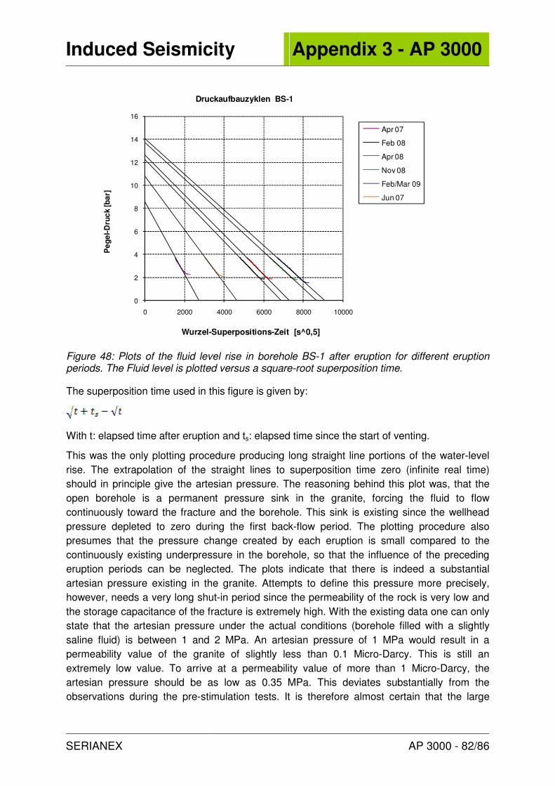
Induced Seismicity Appendix 3 - AP 3000
SERIANEX AP 3000 - 82/86
0
2
4
6
8
10
12
14
16
0 2000 4000 6000 8000 10000
Pe
ge
l-D
ruc
k [b
ar]
Wurzel-Superpositions-Zeit [s^0,5]
Druckaufbauzyklen BS-1
Apr 07
Feb 08
Apr 08
Nov 08
Feb/Mar 09
Jun 07
Figure 48: Plots of the fluid level rise in borehole BS-1 after eruption for different eruption periods. The Fluid level is plotted versus a square-root superposition time.
The superposition time used in this figure is given by:
With t: elapsed time after eruption and ts: elapsed time since the start of venting.
This was the only plotting procedure producing long straight line portions of the water-level rise. The extrapolation of the straight lines to superposition time zero (infinite real time) should in principle give the artesian pressure. The reasoning behind this plot was, that the open borehole is a permanent pressure sink in the granite, forcing the fluid to flow continuously toward the fracture and the borehole. This sink is existing since the wellhead pressure depleted to zero during the first back-flow period. The plotting procedure also presumes that the pressure change created by each eruption is small compared to the continuously existing underpressure in the borehole, so that the influence of the preceding eruption periods can be neglected. The plots indicate that there is indeed a substantial artesian pressure existing in the granite. Attempts to define this pressure more precisely, however, needs a very long shut-in period since the permeability of the rock is very low and the storage capacitance of the fracture is extremely high. With the existing data one can only state that the artesian pressure under the actual conditions (borehole filled with a slightly saline fluid) is between 1 and 2 MPa. An artesian pressure of 1 MPa would result in a permeability value of the granite of slightly less than 0.1 Micro-Darcy. This is still an extremely low value. To arrive at a permeability value of more than 1 Micro-Darcy, the artesian pressure should be as low as 0.35 MPa. This deviates substantially from the observations during the pre-stimulation tests. It is therefore almost certain that the large
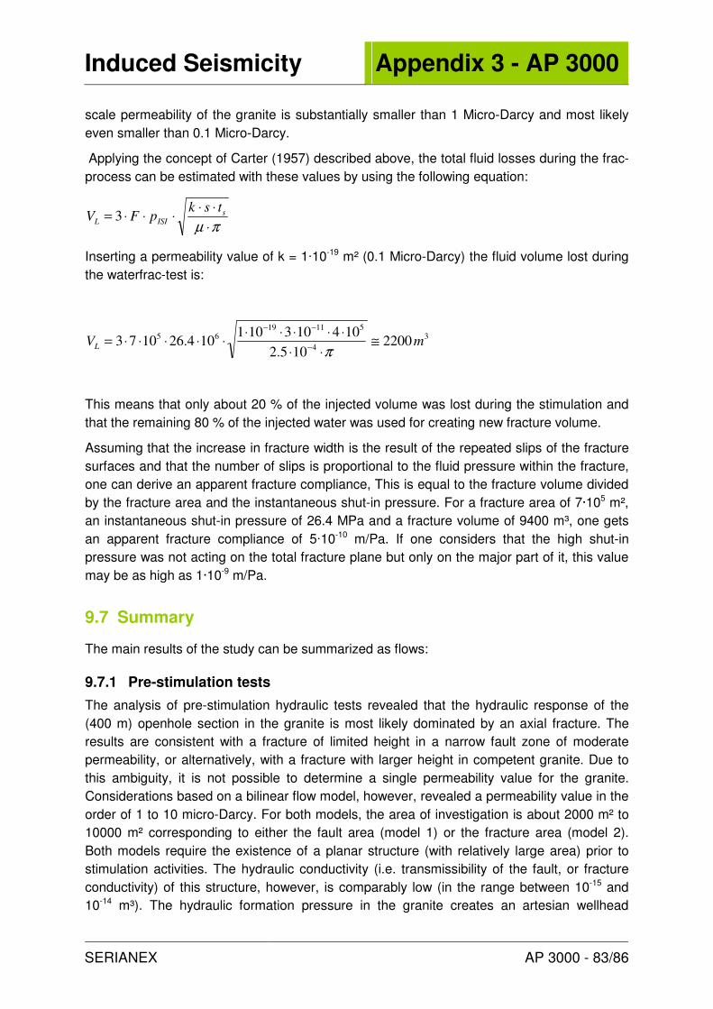
Induced Seismicity Appendix 3 - AP 3000
SERIANEX AP 3000 - 83/86
scale permeability of the granite is substantially smaller than 1 Micro-Darcy and most likely even smaller than 0.1 Micro-Darcy.
Applying the concept of Carter (1957) described above, the total fluid losses during the frac-process can be estimated with these values by using the following equation:
πµ ⋅
⋅⋅⋅⋅⋅= s
ISIL
tskpFV 3
Inserting a permeability value of k = 1·10-19 m² (0.1 Micro-Darcy) the fluid volume lost during the waterfrac-test is:
3
4
51119
652200
105.2
104103101104.261073 mVL ≅
⋅⋅
⋅⋅⋅⋅⋅⋅⋅⋅⋅⋅=
−
−−
π
This means that only about 20 % of the injected volume was lost during the stimulation and that the remaining 80 % of the injected water was used for creating new fracture volume.
Assuming that the increase in fracture width is the result of the repeated slips of the fracture surfaces and that the number of slips is proportional to the fluid pressure within the fracture, one can derive an apparent fracture compliance, This is equal to the fracture volume divided by the fracture area and the instantaneous shut-in pressure. For a fracture area of 7·105 m², an instantaneous shut-in pressure of 26.4 MPa and a fracture volume of 9400 m³, one gets an apparent fracture compliance of 5·10-10 m/Pa. If one considers that the high shut-in pressure was not acting on the total fracture plane but only on the major part of it, this value may be as high as 1·10-9 m/Pa.
9.7 Summary
The main results of the study can be summarized as flows:
9.7.1 Pre-stimulation tests
The analysis of pre-stimulation hydraulic tests revealed that the hydraulic response of the (400 m) openhole section in the granite is most likely dominated by an axial fracture. The results are consistent with a fracture of limited height in a narrow fault zone of moderate permeability, or alternatively, with a fracture with larger height in competent granite. Due to this ambiguity, it is not possible to determine a single permeability value for the granite. Considerations based on a bilinear flow model, however, revealed a permeability value in the order of 1 to 10 micro-Darcy. For both models, the area of investigation is about 2000 m² to 10000 m² corresponding to either the fault area (model 1) or the fracture area (model 2). Both models require the existence of a planar structure (with relatively large area) prior to stimulation activities. The hydraulic conductivity (i.e. transmissibility of the fault, or fracture conductivity) of this structure, however, is comparably low (in the range between 10-15 and 10-14 m³). The hydraulic formation pressure in the granite creates an artesian wellhead

Induced Seismicity Appendix 3 - AP 3000
SERIANEX AP 3000 - 84/86
pressure of 1.5 MPa to 2 MPa when the borehole is filled with water and is in thermal equilibrium with the surrounding rock formations.
There is no indication for a constant pressure or a “no-flow boundary” within the area of investigation.
9.7.2 Stimulation test
During stimulation, the injectivity index of the borehole increased dramatically. Assuming that flow occurred predominantly into a pre-existing fracture, the hydraulic conductivity of this fracture increased by about three orders of magnitude and reached 10-12 m³ at the end of the test. The post-stimulation conductivity was derived from the instantaneous pressure drop after shut-in. Since this pressure drop is a rapid process, the data does not reveal information of the inflow conditions from the well into the fracture and it is not possible to better constrain the fracture conductivity. A fair assumption is that the post-frac fracture conductivity is in the range of 1·10-12 m³ to 1·10-11 m³. The fracture conductivity did not decrease significantly during pressure decline (Jung & Ortiz, 1987).
The record of the injection pressure showed that the increase in fracture conductivity started at a wellhead pressure of about 5 MPa. The irregular trend of the injection pressure during the test clearly indicates that shearing was the dominant stimulation mechanism. Pressure stabilized only during high flow rates at the end of the test, indicating that the elastic response of the fracture became more significant. The pressure observed after the instantaneous pressure drop at shut-in was 26.4 MPa above hydrostatic. This pressure can be regarded as a lower bound for the jacking pressure (pressure in balance with the effective normal stress acting on its surface).
9.7.3 Post-frac observations
Although no significant hydraulic test could be performed after the stimulation test, valuable information could be derived from the pressure decline during shut-in and backflow. The pressure decline observed during the shut-in period could be simulated by using a simple model consisting of a large single fracture with high storage capacitance and high transmissibility, which is loosing fluid into the surrounding homogenous matrix (granite). Using the fracture size determined from the microseismic cloud, the fracture compliance and the permeability of the granite surrounding the fracture (or fault) was determined. With a similar model, the record of the fluid volume during the backflow period could be evaluated. The fracture storage capacitance obtained from these data is approximately 50 m³/MPa for the shut-in period, and approximately 80 m³/MPa for the backflow period. This implies that 50 m³ or 80 m³ of fluid have to flow from the granite into the fracture in order to increase the pressure within the fracture by 1 MPa. The difference between the two values may be attributed to the fact that fracture size increased significantly during the shut-in and the early part of the backflow period.
The fracture storage capacitance can be used to determine the large scale fracture compliance (elastic change of fracture width). Assuming that the fracture size is identical to the area defined by the micro-seismic events, we obtain 8· 10-11 m³/Pa for both cases.

Induced Seismicity Appendix 3 - AP 3000
SERIANEX AP 3000 - 85/86
The large scale permeability value for the granite derived from the shut-in period is 3·10-18 m2. For the backflow period, however, we obtain a value of only 3·10-20 m2. This discrepancy might reflect that the fracture continued to propagate during shut-in. The fluid volume consumed by this process accelerates the pressure decline thus pretending a higher permeability of the rock. The permeability estimate of 3·10-18 m2 is therefore an upper limit for the large scale permeability of the granite. On the other hand, the artesian pressure of 2 MPa assumed for the evaluation of the back-flow period might be overestimated. A value of 1 MPa, for example, would result in a permeability value close to 1·10-19 m². Since it is unlikely that the artesian pressure under the prevailing conditions is significantly lower than 1 MPa, it is almost certain that the large scale permeability of the granite is substantially smaller than 1 Micro-Darcy and most likely even smaller than 0.1 Micro-Darcy. It should be mentioned that the permeability would be even smaller when the “hydraulic” fracture size is larger than the seismically active fracture area. An assumption that is not unreasonable.
Fluid balance considerations based on the results for a permeability value of 1·10-19 m² show that during the stimulation test the majority of the injected fluid (about 80 %) was required for creating new fracture volume and that a much smaller part permeated into the matrix (granite). The hydraulic parameter values determined by this study are listed in the Table 6.
Of primary importance for the current study is the question whether or not the fracture (in its current state) might be connected to a larger scale hydraulic feature (e.g. major fault). Within the radius of investigation (approximately 1500 m) there is no indication for a constant pressure boundary and a connection to a highly conductive larger scale feature can almost certainly be excluded.
Another important question concerning the triggering of post-injection seismicity is, to what extend the reservoir has been over-pressurized in the post-injection period. It had been suspected that the eruptive overflow of the borehole persisting until today might be driven by the relict of the overpressure created during stimulation. Unfortunately, no long term pressure build-up recordings exist for the post-stimulation period and information on hydraulic overpressures can only be obtained indirectly from outflow recordings. Analysis of this data indicates that the overpressure in the bulk of the reservoir might not be higher than the artesian pressure. However, since stimulation is a non-reversible process, it can not be excluded that in parts of the reservoir the pressure decline took much longer than the pressure build-up and that overpressures resulting from the stimulation may persist for a significantly longer period of time. In this case, hydraulic overpressures might also be responsible for the post-injection seismicity observed at the outer rim of the stimulated area.

Induced Seismicity Appendix 3 - AP 3000
SERIANEX AP 3000 - 86/86
Parameter Unit Range
possible
Range
likely
Large scale permeability of the granite m² 3·10-20 - 1·10-17 3·10-20 - 1·10-19
Storage coefficient of the granite (assumed)
1/Pa 1·10-11 - 1·10-10 1·10-11
Pre-frac artesian pressure MPa 1.5 – 2.5 1.5 – 2
Post-frac artesian pressure MPa 0.2 – 2.5 1 – 2
Pre-frac fracture conductivity m³ 1·10-13 – 3·10-16 1·10-14 – 1·10-15
Pre-frac fault transmissibility m³ 1·10-16 – 1·10-15 1·10-15
Post-frac fracture conductivity m³ 1·10-12 - 1·10-11 1·10-12
Fracture compliance (elastic response) m/Pa 5·10-11 - 1·10-10 8·10-11
Fracture compliance simulating fracture opening during stimulation
m/Pa 5·10-10 -1·10-9 5·10-10 -1·10-9
wellhead pressure for the onset of shearing
MPa 5 5
wellhead jacking pressure MPa ≥ 26.4 ≥ 26.4
Table 6: Summary of the hydraulic parameters.