series solutions of partial differential equations using ... · pdf filethe complex integral...

International Mathematical Forum, Vol. 9, 2014, no. 31, 1477 - 1494

HIKARI Ltd, www.m-hikari.com

http://dx.doi.org/10.12988/imf.2014.48145

Series Solutions of Partial Differential Equations

Using the Complex Integral Method

W. Robin

Engineering Mathematics Group

Edinburgh Napier University

10 Colinton Road, EH10 5DT, UK Copyright © 2014 W. Robin. This is an open access article distributed under the Creative

Commons Attribution License, which permits unrestricted use, distribution, and reproduction in

any medium, provided the original work is properly cited.

Abstract

The complex integral method for solving ordinary differential equations in series

[3, 7, 8] is extended to cover the series solution of partial differential equations

also. The means of this extension is straightforward, with both ‘ordinary’ and

‘Frobenius’ multiple variable power series being dealt with. Standard examples of

the application of the extended method(s) to first-order, second-order, third-order

and simultaneous partial differential equations are provided throughout. Examples

also include the series solution of a non-linear partial differential equation and the

consideration of series solutions with negative powers.

Mathematics Subject Classification: 30B10, 30E20, 32A05, 32A30, 35A25,

35C10, 35F10, 35F25, 35G10

Keywords: Partial differential equations, several complex variables, series

solutions, complex integrals

1. Introduction

In this paper we extend the application of the complex integral method for solving

ordinary differential equations (ODE) in series [3, 7, 8] to cover the power series

solution of partial differential equations (PDE) also. The means of this extension,

1478 W. Robin

from the single independent variable to the several independent variables case, is

quite straightforward, as we simply apply the procedure variable by variable to the

particular assumed multiple variable series format in each case, with both the

‘ordinary’ and ‘Frobenius’ multiple variable series being dealt with. The method,

as it is developed, is used to provide series solutions to first-order, second-order

and third-order PDE and, in addition, we consider the solution of simultaneous

PDE. As an added point of interest, we extend the method, when required, to the

consideration of series solutions with negative powers.

There are, of course, certain differences when we enter the realm of PDE. For

a start, it is of the nature of the complex integral method to produce particular

solutions [7, 8]. Also, there is the problem of accounting for boundary or initial

conditions; these must be dealt with in a manner consistent with the complex

integral method itself. In addition to these general points, there is the practical

difficulty that the recurrence relations determining the coefficients of the series

solutions will be multi-variable and multi-term. And, then, if a series solution is

possible, there is the ever-present (multi-variable) convergence problem. These

points aside, the actual ‘mechanics’ of the solution process remains the same as in

the ODE case: the PDE is effectively replaced by a system of (uncoupled) simple

equations in one (discrete) variable, through a purely formal process.

The paper is organized as follows. In section 2 we develop the complex

integral method for the solution in series of PDE in two independent variables

about two ordinary points. This is followed, in section 3, by some standard

examples of first-order PDE, including a nonlinear PDE and simultaneous PDEs

in two independent variables, while, in section 4, we solve some standard

examples of second-order PDE in two independent variables. In section 5 we

develop the complex integral method for the solution of PDE in series with three

independent variables and apply it to obtain a particular solution of Laplace’s

equation. The complex integral method for solution in series of PDE with two

independent variables is itself extended, in section 6, to the case of Frobenius

series in two independent variables, including the case of PDE where a series

solution with negative powers is required, and used in the solution of certain

standard examples. The paper is rounded-off with a short conclusions and

discussion section, section 7.

2. The Basic Formalism for Two Independent variables

When seeking series solutions to ODE, using the complex integral method [3], we

consider that the solution )(zf may be expressed as an infinite series about an

ordinary point, ,0z of the form [4]

Series solutions of PDE using the complex integral method 1479

m

m

m zzazf )()( 0

0

(2.1)

with the coefficients 0}{ mma given by Herrera’s complex integral formula as [3]

Ckm

k

km dz

zz

zf

iπma

1

0

)(

)(

)(

2][

1 (2.2)

with C an appropriate closed contour [3] and where, following Ince [4], we write

)1()2)(1(][ kmmmmm k (2.3)

where ,,3,2,1, kkkkm and .,3,2,1,0 k

When seeking to extend the complex integral method to PDEs, it is necessary

to apply the basic complex integration process, successively, variable by variable.

To see how this works, suppose that we seek a series solutions to a PDE with two

variables, that is, we assume that the solution of our PDE, ),,( 21 zzf may be

expressed as an infinite series about two ordinary points, 01z and ,02z of the form

0 0

022011,21 )()(),(i j

jiji zzzzazzf (2.4)

Then, with

21

2121

),( ),(),(

zz

zzfzzf

k

kk

(2.5)

and ),,(),( 2121)0,0( zzfzzf we can differentiate (2.3) to get

ki j

jkijik

k zzzzajizzf

)()(][][),( 022011,21),(

(2.6a)

Or

nkm

nmkk zzzzanmzzf )()(][][),( 022011,21

),(

mki nj

jkijik zzzzaji

)()(][][ 022011, (2.6b)

Finally, dividing through (2.6b) by 1

0221

011 )()( nkm zzzz and integrating

round appropriate closed contours, 2C and ,1C with respect to 2z and then ,1z we

find that

1480 W. Robin

nmk

C Cn

k

kmanmi

zz

zzfdz

zzdz ,

2

1 2

1022

21),(

21011

1 ][][)ˆ2()(

),(

)(

1

(2.7)

where (2.6) follows from the standard result [7] that, if is an integer and 1ˆ2 i

otherwise ,0

1 ˆ2)( 0

n, iπdzzz

C

(2.8)

where z is a complex variable and 0z a fixed point within the closed contour .C

Looking back, we see that ,,3,2,1, kkkkm .,3,2,1,0 k and

,,3,2,1, n .,3,2,1,0

Apparently, if we have higher-order (than second-order) PDE, the formula

(2.7) expands accordingly, in an obvious manner (see section 5 below).

With PDE, the boundary or initial conditions play an active role in the solution

process and it will prove necessary, following [2, 5, 6], to transform the boundary

or initial conditions along with the PDE. To do this we assume that the boundary

or initial conditions are analytic functions of the variables and use the complex

integral formulas (2.2) or (2.7) or their logical extension (when necessary) to

transform them along with the PDE. As mentioned, this process follows [2, 5, 6]

and becomes more transparent as the examples presented below are worked-

through.

Before we move-on to the next section, it is convenient, at this point, to recall

the definition of the Kronecker delta function, which we write in our notation as

,, ji with

ji if ,1

ji if 0,

, ji (2.9)

The Kronecker delta function plays a not insignificant role in what follows.

3. First-Order PDE with Two Independent Variables

In this and the following section, we present a number of examples, including

some from the literature involving the differential transform method, which acts

as benchmark or comparison for the current method, involving PDE with two

independent variables. We transform the original notations into the standard

notation we have introduced above and assume, henceforth, that .00201 zz

For our first example, we consider the first-order linear PDE [2]


2121)1,0(

21)0,1(

1 ),(),( zzzzfzzfz (3.1)

subject to the conditions

0)0,(0

10,1)0,0(

i

ii zazf and 0),0(

02,02

)0,0(

j

jj zazf (3.2)

We now divide through (3.1) by 1

21

1 ji zz and integrate round appropriate closed

contours, 2C and ,1C with respect to 2z and then ,1z to get (using (2.8))

21,1,

1 2

12

21)1,0(

211

1

1 2

12

21)0,1(

2

1

1 )ˆ2(),(1),(1

iz

zzfdz

zdz

z

zzfdz

zdz ji

C Cji

C Cji

(3.3)

The next step is to compare the integrands of (3.3) with the general result (2.7),

when we find that (3.3) is transformed into

1,1,1,, )1( jijiji ajia (3.4)

We now divide through the conditions (3.2) by 1

1iz or

12j

z and integrate round an

appropriate closed contours, 1C or ,2C with respect to 1z or ,2z to get

0)0,(

1

111

1)0,0(

C

idz

z

zf and 0

),0(

2

212

2)0,0(

C

jdz

z

zf (3.5)

or, from (2.7) and (3.2)

00, ia and 0,0 ja (3.6)

With (3.4) and (3.6) we have effectively recovered the solution of Chen and Ho

[2], and it is a straightforward matter to check that (by mathematical induction)

,4,3,2 ,!

1)1(

,1 j

ja j

j (3.7)

and 0, jia otherwise, so that the solution of (3.1) subject to (3.2) is

2

2121 )1(),(j

jj zzzzf (3.8)

For our next example, we consider the first-order nonlinear PDE [5]

1482 W. Robin

0),(),(),( 21)0,1(

21)0,0(

21)1,0( zzfzzfzzf (3.9)


1

0

10,1)0,0( )0,( zzazf

i

ii

(3.10a)

and

0),0(0

2,02)0,0(

j

jj zazf (3.10b)

We now divide through (3.9) by 1

21

1 ji zz and integrate round appropriate closed

contours, 2C and ,1C with respect to 2z and then ,1z to get (using (2.4))

1 2

12

21)1,0(

211

1

),(1

C Cji

z

zzfdz

zdz

0),(1

0 01 2

12

21)0,1(

211

1,

s r C Csjrisr

z

zzfdz

zdza (3.11)

Comparing the integrands of (3.11) with the general result (2.7), we find that

(3.11) is transformed into

0)1()1(0 0

,1,1,

j

s

i

r

sjrisrji ariaaj (3.12)

Meanwhile, from the conditions (3.10a) we get

10,1 a and 00. ia otherwise (3.13)

and condition (3.10b) is then an identity. Substituting (3.13) into (3.12), we find

that

0)1(0

,1,11,1

j

s

sjsj aaaj (3.14)

so that, on combining (3.13) and (3.14), the solution of our difference problem

(3.12) with (3.13) is

otherwise 0,

1 ,)1(,

iifa

j

ji for ,3,2,1,0j (3.15)

Finally, from (3.15) the solution of (3.9), subject to the conditions (3.10), is


2

1

02121

1)1(),(

z

zzzzzf

j

jj

(3.16)

in agreement with Jang et al [5] (and (3.9) and (3.10)).

The complex integral method may be applied to systems of PDE with equal

facility as its application to individual PDE. Consider the following system of

first-order PDE [6]

0),(),(),(),( 21)0,0(

21)0,0(

21)0,1(

21)1,0( zzgzzfzzgzzf (3.17a)

and

0),(),(),(),( 21)0,0(

21)0,0(

21)0,1(

21)1,0( zzgzzfzzfzzg (3.17a)

where

0 0

21,21 ),(i j

jiji zzazzf and

0 0

21,21 ),(i j

jiji zzbzzg (3.17c)

subject to the conditions that

0

121

11)0,0(

)!12()sinh()0,(

i

i

i

zzzf (3.18a)

and

0

21

11)0,0(

)!2()cosh()0,(

i

i

i

zzzg (3.18b)

The complex integral method is applied as above. Starting with (3.17a) and

(3.17b), we divide through by ,1

21

1 ji zz integrate round appropriate closed

contours, 2C and ,1C with respect to 2z and then ,1z and then compare the

resulting integrands with the general result (2.7), when we find that equations

(3.17a) and (3.17b) are transformed into

0)1()1( ,,,11, jijijiji babiaj (3.19a)

and

0)1()1( ,,,11, jijijiji baaibj (3.19b)

Next, we divide through (3.18a) and (3.18b) by ,11iz integrate round an

appropriate closed contour, ,1C with respect to ,1z and then compare the resulting

1484 W. Robin

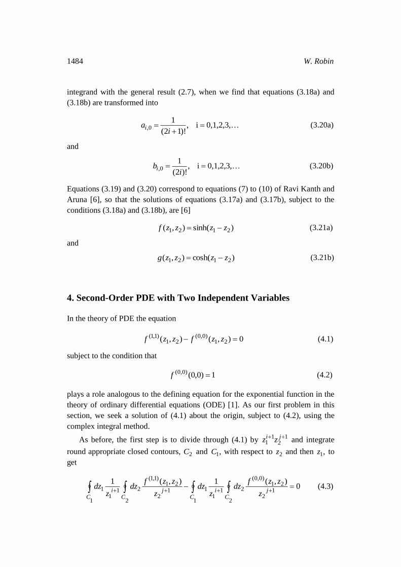
integrand with the general result (2.7), when we find that equations (3.18a) and

(3.18b) are transformed into

0,1,2,3,i ,)!12(

10,

iai (3.20a)

and

0,1,2,3,i ,)!2(

10,

ibi (3.20b)

Equations (3.19) and (3.20) correspond to equations (7) to (10) of Ravi Kanth and

Aruna [6], so that the solutions of equations (3.17a) and (3.17b), subject to the

conditions (3.18a) and (3.18b), are [6]

)sinh(),( 2121 zzzzf (3.21a)

and

)cosh(),( 2121 zzzzg (3.21b)

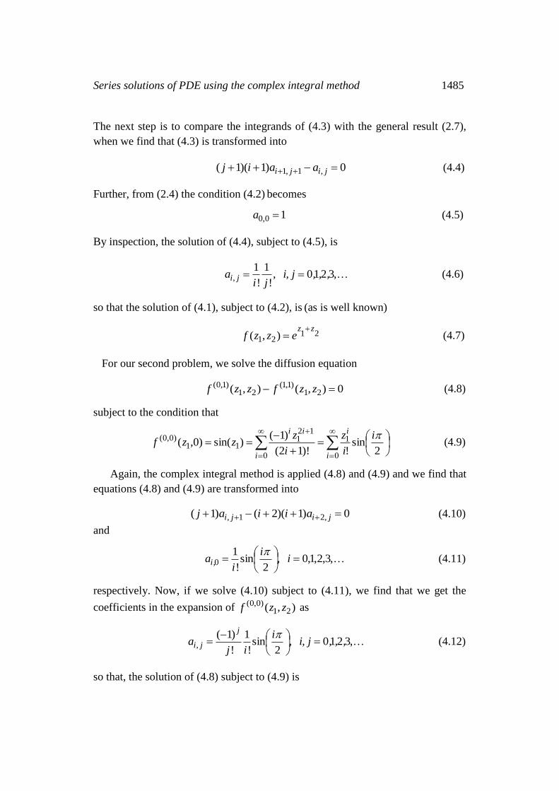
4. Second-Order PDE with Two Independent Variables

In the theory of PDE the equation

0),(),( 21)0,0(

21)1,1( zzfzzf (4.1)

subject to the condition that

1)0,0()0,0( f (4.2)

plays a role analogous to the defining equation for the exponential function in the

theory of ordinary differential equations (ODE) [1]. As our first problem in this

section, we seek a solution of (4.1) about the origin, subject to (4.2), using the

complex integral method.

As before, the first step is to divide through (4.1) by 1

21

1 ji zz and integrate

round appropriate closed contours, 2C and ,1C with respect to 2z and then ,1z to

get

0),(1),(1

1 2

12

21)0,0(

211

1

1 2

12

21)1,1(

211

1 C C

jiC C

jiz

zzfdz

zdz

z

zzfdz

zdz (4.3)


The next step is to compare the integrands of (4.3) with the general result (2.7),

when we find that (4.3) is transformed into

0)1)(1( ,1,1 jiji aaij (4.4)

Further, from (2.4) the condition (4.2) becomes

10,0 a (4.5)

By inspection, the solution of (4.4), subject to (4.5), is

,3210 ,!

1

!

1

, ,,,ji,

jia ji (4.6)

so that the solution of (4.1), subject to (4.2), is (as is well known)

2121 ),(

zzezzf

(4.7)

For our second problem, we solve the diffusion equation

0),(),( 21)1,1(

21)1,0( zzfzzf (4.8)

subject to the condition that

2sin

!)!12(

)1()sin()0,(

0

1

0

121

11)0,0( i

i

z

i

zzzf

i

i

i

ii

(4.9)

Again, the complex integral method is applied (4.8) and (4.9) and we find that

equations (4.8) and (4.9) are transformed into

0)1)(2()1( ,21, jiji aiiaj (4.10)

and

,3,2,1,0 ,2

sin!

1

0

i

i

iai,

(4.11)

respectively. Now, if we solve (4.10) subject to (4.11), we find that we get the

coefficients in the expansion of ),( 21)0,0( zzf as

,3210 ,2

sin!

1

!

)1(

, ,,,ji,

i

ija

j

ji

(4.12)

so that, the solution of (4.8) subject to (4.9) is

1486 W. Robin

)sin(),( 12

21 zz

ezzf

(4.13)

Naturally, we can obtain the solutions of the last two examples by separation of

variables, a much easier proposition in these cases.

Our third example [2] involves the solution of the second-order PDE

0),(),( 21)0,2(2

21)2,0( zzfczzf (4.14)

with c a constant (the wave equation), subject to the conditions

31

0

10,1)0,0( )0,( zzazf

i

ii

and 1

0

11,1)1,0( )0,( zzazf

i

ii

(4.15)

As before, we divide through (4.14) by 1

21

1 ji zz and integrate round appropriate

closed contours, 2C and ,1C with respect to 2z and then ,1z to get

0),(1),(1

1 2

12

21)0,2(

211

12

1 2

12

21)2,0(

211

1 C C

jiC C

jiz

zzfdz

zdzc

z

zzfdz

zdz (4.16)

Once again, the next step is to compare the integrands of (4.16) with the general

result (2.7), when we find that (4.16) is transformed into

0)1)(2()1)(2( 1,2

2, jiji aiicajj (4.17)

Next, we divide through the conditions (4.15) by 1

1iz and integrate round an

appropriate closed contour, ,1C with respect to 1z when we get

1

111

31

1

111

1)0,0( )0,(

Ci

Ci

dzz

zdz

z

zf and

1

111

1

1

212

1)1,0( )0,(

Ci

Ci

dzz

zdz

z

zf (4.18)

or, from (2.8) and (4.15)

3,0, iia and 1,1, iia (4.19)

From (4.17) and (4.19) and mathematical induction we find that the only nonzero

coefficients are ,10,3 a 11,1 a and ,3 22,1 ca in agreement with [2]. This

means that the (non-separable) solution of (4.14) satisfying the conditions (4.15)

is [2]

31

221

22121 3),( zzzczzzzf (4.20)


For our last example in this section, following [2] again, we consider the

second-order PDE

121)0,0(

121)0,2(

21)2,0( ),(),(),( zzzfzzzfzzf (4.21)


0)0,(0

10,1)0,0(

i

ii zazf and 0)0,(

0

11,1)1,0(

i

ii zazf (4.22)

Following the previous procedure, we find that (4.21) and (4.22) transform into

the difference equation

0,1,,21,2, )1)(2()1)(2( jijijiji aaiiajj (4.23)

subject to the conditions that

00, ia and 01, ia (4.24)

It is straightforward to check that the first few nonzero coefficients are

,2

12,1 a

120

16,1 a and

24

14,3 a (4.25)

in agreement with [2] again, so that the first few terms of the solution of the initial

value problem (4.21)/(4.22) are [2]

120242

),(621

42

31

221

21

zzzzzzzzf (4.26)

5. Second-Order PDE with Three Independent Variables

We assume that the solution, ),,,( 321 zzzf of our PDE with three independent

variables may be expressed as an infinite series about three ordinary points, ,01z

02z and ,03z of the form

0 0 0

033022011,,321 )()()(),,(i j l

ljilji zzzzzzazzzf (5.1)

Then, with

321

321321

),,( ),,(),,(

zzz

zzzfzzzf

kh

khkh

(5.2)

1488 W. Robin

and ),,,(),,( 321321)0,0,0( zzzfzzzf we can differentiate (5.1) to get

hi kj l

lkjhijikh

kh zzzzzzaljizzzf

)()()(][][][),,( 033022011,321),,(

---------- (5.3a)

or

pknhm

pnmkhkh zzzzzzapnmzzzf )()()(][][][),,( 033022011,,321

),,(

mhi nkj pl

lkjhijikh zzzzzzalji

)()()(][][][ 033022011, (5.3b)

Finally, dividing through (5.3b) by

1

0331

0221

011 )()()( pknhm zzzzzz

and integrating round appropriate closed contours, ,3C 2C and ,1C with respect to

,3z 2z and then ,1z we find that

1 2 3

1033

321),,(

31022

11011 )(

),,(

)(

1

)(

1

C C Cl

kh

knhm zz

zzzfdz

zzdz

zz

pnmkh apnmi ,,3 ][][][)ˆ2( (5.4)

where (5.4) follows from the standard result (2.8). Equation (5.4) is a straight-

forward generalization of equation (2.7).

We restrict ourselves to the single example of solving a PDE with three

independent variables; we consider Laplace’s equation

0),,(),,(),,( 321)2,0,0(

321)0,2,0(

321)0,0,2( zzzfzzzfzzzf (5.5)

subject to the condition

1)0,0,0()0,0,0( f (5.6)

As before, we now take ,0030201 zzz and following the basic method, we

divide through (5.5) by 13

12

11

lnm zzz , and integrate to get

1 2 3

13

321)0,0,2(

312

111

),,(11

C C Clnm z

zzzfdz

zdz

z


1 2 3

13

321)0,2,0(

312

111

),,(11

C C Clnm z

zzzfdz

zdz

z

0),,(11

1 2 3

13

321)2,0,0(

312

111

C C C

lnm z

zzzfdz

zdz

z (5.7)

which, on comparison with (5.4), reduces to

0)1)(2()1)(2()1)(2( 2,,,2,,,2 ljiljilji allajjaii (5.8)

Now, from (5.1) we see that (5.6) becomes

10,0,0 a (5.9)

and, by inspection, we see that the solution of (5.8), subject to (5.9), is

,3,2,1,0,, ,!

1

!!

1

,, lji

lj

i

ia lji (5.10)

and recognize, via (5.1), that the solution of (5.5), subject to (5.6), is

321321 ),,(

zzzezzzf

(5.11)

As in two previous examples, the solution (5.11) of (5.5), subject to (5.6), is a

variable separable solution.

6. Solution of PDE Using Frobenius Series

In this section we consider the extension of the complex integral method to the

solution of PDE in two independent variables through (initially) the assumption

that the solution of the PDE has the form of a ‘double’ Frobenius series, that is

0 0

022011,21 )()(),(i j

sjriji zzzzazzf (6.1)

where, by an analogous argument to that of section 2, we find that

nmk

C Csn

k

krmasnrmi

zz

zzfdz

zzdz ,

2

1 2

1022

21),(

21011

1 ][][)ˆ2()(

),(

)(

1

(6.2)

1490 W. Robin

As a first example of this approach to the solution of PDE, we consider, again

equation (4.1) [1] (written slightly differently)

),(),( 21)0,0(

21)1,1( zzfzzf (6.3)

Applying the usual integration approach with ,00201 zz but dividing (6.3) by

12

11

sjri zz this time, we integrate through (6.3) to get

1 2

12

21)0,0(

211

1

1 2

12

21)1,1(

211

1 ),(),(

C Csnrm

C Csnrm z

zzfdz

z

dz

z

zzfdz

z

dz (6.4)

which, on comparison with (6.2), reduces to

jiji aasjri ,1,1)1)(1( (6.5a)

or

1,1,))(( jiji aasjri (6.5b)

Equation (6.5b) is the recurrence relation for our assumed Frobenius series

solution (6.1). To get the associated indicial equation, we set 0 ji in (6.5b)

and, with ,00,0 a we see that the indicial equation for (6.3) is

0rs (6.6)

so that either 0 sr (covered already), or 0r while s is arbitrary, or 0s

while r is arbitrary. Following [1], we may take it that the general solution will, in

some way, follow as a linear superposition of all three possible solution types. As

we have considered the 0 sr case already, we look next at the 0s while r is

arbitrary case. From (6.5b) with ,0s we get

jri

aa

jiji

)(

1,1,

(6.7)

so that we get the first few coefficients, recursively, as

,0,0a ,1).1(

0,01,1

r

aa

,

2.1).2)(1(

0,02,2

rr

aa

(6.8)

At this point we are at liberty to choose particular forms for 0,0a and ,r so we

follow Chaundy [1] and choose ,1

0,0

aa

r when (4.8) becomes


,1

a ,

1).1(

11,1

aaa ,

2.1).2)(1(

12,2

aaaa (6.9)

and the first few terms of a particular solution of (6.3) are then

2.1).2)(1(1).1(),(

22

212

111

21aaa

zz

aa

zz

a

zzzf

aaa

a

(6.10)

When we consider the other option, with 0r while s is arbitrary, we get a

(third) series which, on choosing ,1

0,0

ba

s can be written as

)2)(1(.2.1)1(.1),(

22

21

1212

21bbb

zz

bb

zz

b

zzzf

bbb

b (6.11)

It follows that linear superposition of (4.7) ( 0 sr ), (6.10) and (6.11) will

produce a more general solution of the linear PDE (6.3).

Sometimes we require a Frobenius series with decreasing powers [1], for

example

0 0

022011,21 )()(),(i j

sjriji zzzzazzf (6.12)

where, by an analogous argument to that of section 2, we find that

nmk

C Csn

k

krmasnrmi

zz

zzfdz

zzdz ,

2

1 2

1022

21),(

21011

1 ][][)ˆ2()(

),(

)(

1

---------- (6.13)

As an example of the application of (6.12) and (6.13), we consider, again, the

diffusion equation

0),(),( 21)0.2(

21)1,0( zzfzzf (6.14)

Dividing through (6.14) by 1

21

1 sjri zz and integrating through as usual we find

that (6.14) becomes

0),(),(

1 2

12

21)0,2(

211

1

1 2

12

21)1,0(

211

1 C C

sjriC C

sjriz

zzfdz

z

dz

z

zzfdz

z

dz (6.15)

which equation, on comparison with (6.13), reduces to the recurrence relation

1492 W. Robin

1,,2 )1()1)(2( jiji asjariri (6.16a)

or

1,2, )1()1)(( jiji asjariri (6.16b)

Setting 0 ji in (6.16b), we get, with ,00,0 a the indicial equation

0)1( rr (6.17)

so that 0r or ,1r with s arbitrary. To get the first series solution to (6.14), we

set 0r in (6.16b) and, with ,10,0 a we solve (6.16b) recursively find that the

first few terms of the first solution (6.12) to (6.14) are

32

61

22

41

12

21

221

!6

)2)(1)((

!4

)1)((

!2

)()( ssss zz

ssszz

sszz

sz,zzf

---------- (6.18)

with the full series being given by Chaundy [1]. Similarly, to get the second

Frobenius series solution to (6.14), we set 1r in (6.16b) and, with ,10,0 a we

solve (6.16b) recursively find that the first few terms of the second solution (6.12)

to (6.14) are

32

71

22

51

12

31

2121

!7

)2)(1)((

!5

)1)((

!3

)()( ssss zz

ssszz

sszz

szz,zzf

---------- (6.19)

with (again) the full series being given by Chaundy [1], who also exposes the

relationship between the two series (6.18) and (6.19).

7. Discussion and Conclusions

Herrera’s complex integral method appears to have sufficient flexibility to enable

its generalization to the production of (power) series solutions to most types of

differential equation. The extension processes appear ‘natural’ and the overall

(formal) simplicity of the ‘reduction’ of the original equation or equations to a

system of uncoupled simple equations in one variable is maintained throughout

the various types of extension. The three main problems of the method, con-

vergence of the series, solution of the recurrence relation and the provision of

particular solutions only, are endemic to the power series approach anyway, and

are shared by all other power series approaches to the solution of differential

equations, for example, the differential transform method [2, 5, 6].


Many of the examples considered here were taken from papers using the

differential transform method of solution of differential equations [2, 5, 6]. While

both the differential transform method and the complex integral method yield the

same answers in the situations where the differential transform method applies,

the complex integral method is, I feel, easier to use, the methodology springing, as

it does, from the general properties of the (complex) integral, as well as the basic

integral ‘Herrera’ results (2.2), (2.7) and so on. In addition, the complex integral

method generalizes, in an obvious manner, to encompass solutions of PDE

inFrobenius series and series with negative powers. Indeed, Herrera’s complex

integral representation of the derivative of a function [3] seems like a natural

generalization of the basic idea of the differential transform concept also.

Some general remarks on the applications considered above seem appropriate

at this point in the discussion. First, the conditions accompanying the PDE that we

solved in sections three to six were all quite simple, with the problems all being

initial value problems. As shown in Jang et al [5], who apply the differential

transform method, boundary value problems are amenable to the series methods

considered here as well. Secondly, the complex integral method is quite capable

of handling PDE with an arbitrary number of independent variables and general-

order derivatives. The generalization of the formulae presented here is quite

straightforward, as we have already pointed out. Thirdly, when tackling PDE it

may often be the case that a search for similarity variables will prove fruitful. For

example, in solving the diffusion equation, (6.14), in section 6, it is useful to

know of the existence of the similarity variable 12 / zz or, as was actually

assumed, ./ 122 zz

In conclusion, we have extended the complex integral method for solving

ordinary differential equations in series [3, 7, 8] to cover the series solution of

partial differential equations also. We have presented examples of the application

of the extended method(s) to first-order, second-order, third-order, non-linear and

simultaneous partial differential equations. Examples [1] involving the Frobenius’

series solution of PDE, including the consideration of series solutions with

negative powers, were also presented. A brief comparison with the differential

transform method [2, 5, 6] has been given and the possibility of further

applications of the complex integral method mentioned.

1494 W. Robin

References

[1] Chaundy T. W.: A Method of Solving Certain Linear Partial Differential

Equations. Proc. London Math. Soc. Series 2, 21 (1923) 214-234.

[2] Chen K.C. and Ho S.H.: Solving partial differential equations by two-

dimensional differential transform method. App. Math. Comp. 106 (1999)

171-179.

[3] Herrera J. C.: Power series solutions in nonlinear mechanics.

Brookhaven National Laboratory Report 37494. Undated.

[4] Ince E. L.: Ordinary Differential Equations. Dover, New York (1956).

[5] Jang M-J., Chen C-L. and Liu Y-C.: Two-dimensional differential transform

for partial differential equations. App. Math, Comp. 121 (2001) 261-270.

[6] Ravi Kanth A.S.V. and Aruna K.: Differential transform method for solving

linear and non-linear systems of partial differential equations. Phys. Lett. A

372 (2008) 6896–6898.

[7] Robin W.: Series Solution of Second-Order Linear Homogeneous Ordinary

Differential Equations via Complex Integration. International Mathematical

Forum 9 (2014) 967-976.

[8] Robin W.: Frobenius Series Solution of Fuchs Second-Order Ordinary

Differential Equations via Complex Integration. International Mathematical

Forum 9 (2014) 953-965.

Received: August 7, 2014

series solutions of partial differential equations using ... · pdf filethe complex integral...

Documents