One-Sample t-TestExample 1: Mortgage Process TimeProblemA faster loan processing time produces higher productivityand greater customer satisfaction. A financial servicesinstitution wants to establish a baseline for their process by

Data setMortgage.MPJ

DescriptionVariableestimating their mean processing time. They also want to

Loan application numberLoandetermine if their mean time differs from a competitor’s claimof 6 hours. Number of hours until customer receives notificationHours

Data collectionA financial analyst randomly selects 7 loan applications andmanually calculates the time between loan initiation and whenthe customer receives the institution’s decision.

Tools

• Descriptive Statistics

• 1-Sample t

• Normality Test

• Time Series Plot

• Individual Value Plot

Hypothesis Tests: Continuous Data 106

One-Sample t-Test

TRMEM180.SQMEI.1

Displaying descriptive statisticsUse descriptive statistics to summarize important features ofthe data. In particular, descriptive statistics provide usefulinformation about the location and variability of the data.

Display Descriptive Statistics1. Open Mortgage.MPJ.

2. Choose Stat > Basic Statistics > Display DescriptiveStatistics.

3. In Variables, enter Hours.

4. Click OK.

Hypothesis Tests: Continuous Data 107

One-Sample t-Test

TRMEM180.SQMEI.1

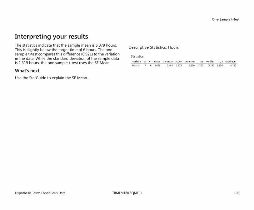
Interpreting your resultsThe statistics indicate that the sample mean is 5.079 hours.This is slightly below the target time of 6 hours. The onesample t-test compares this difference (0.921) to the variationin the data. While the standard deviation of the sample datais 1.319 hours, the one sample t-test uses the SE Mean.

What's nextUse the StatGuide to explain the SE Mean.

Hypothesis Tests: Continuous Data 108

One-Sample t-Test

TRMEM180.SQMEI.1

Standard Error of the MeanWe can see that the SE Mean is simply the standard deviationdivided by the square root of the number of data points andrepresents the dispersion or variation in the distribution ofsample means. The one-sample t-test uses the distribution ofthe sample mean (not the distribution of the data) for theanalysis. Therefore, the standard error of the mean will beused as the estimate of variation for the t-test and confidenceinterval.

Hypothesis Tests: Continuous Data 109

One-Sample t-Test

TRMEM180.SQMEI.1

Hypothesis testingWhat is a hypothesis testA hypothesis test uses sample data to test a hypothesis aboutthe population from which the sample was taken. Theone-sample t-test is one of many procedures available forhypothesis testing in Minitab.

Why use a hypothesis testHypothesis testing can help answer questions such as:

• Are turn-around times meeting or exceeding customerexpectations?

• Is the service at one branch better than the service at another?For example, to test whether the mean duration of atransaction is equal to the desired target, measure the durationof a sample of transactions and use its sample mean to

For example,

• On average, is a call center meeting the target time to answercustomer questions?

estimate the mean for all transactions. Using information froma sample to make a conclusion about a population is knownas statistical inference. • Is the mean billing cycle time shorter at the branch with a new

billing process?When to use a hypothesis testUse a hypothesis test to make inferences about one or morepopulations when sample data are available.

Hypothesis Tests: Continuous Data 110

One-Sample t-Test

TRMEM180.SQMEI.1

One-sample t-testWhat is a one-sample t-testA one-sample t-test helps determine whether μ (thepopulation mean) is equal to a hypothesized value (the testmean).

Why use a one-sample t-testA one-sample t-test can help answer questions such as:

• Is the mean transaction time on target?

• Does customer service meet expectations?The test uses the standard deviation of the sample to estimateσ (the population standard deviation). If the differencebetween the sample mean and the test mean is large relative

For example,

• On average, is a call center meeting the target time to answercustomer questions?

to the variability of the sample mean, then μ is unlikely to beequal to the test mean.

• Is the billing cycle time for a new process shorter than thecurrent cycle time of 20 days?When to use a one-sample t-test

Use a one-sample t-test when continuous data are availablefrom a single random sample.

The test assumes the population is normally distributed.However, it is fairly robust to violations of this assumption forsample sizes equal to or greater than 30, provided theobservations are collected randomly and the data arecontinuous, unimodal, and reasonably symmetric (see [1]).

Hypothesis Tests: Continuous Data 111

One-Sample t-Test

TRMEM180.SQMEI.1

Testing the null hypothesisThe company wants to determine whether the mean time forthe approval process is statistically different from thecompetitor’s claim of 6 hours. In statistical terms, the processmean is the population mean, or μ (mu).

1-Sample t1. Choose Stat > Basic Statistics > 1-Sample t.

2. Complete the dialog box as shown below.Statistical hypothesesEither μ is equal to 6 hours or it is not. You can state thesealternatives with two hypotheses:

The null hypothesis (H0): μ is equal to 6 hours.

The alternative hypothesis (H1): μ is not equal to 6 hours.

Because the analysts will not measure every loan request inthe population, they will not know the true value of μ.However, an appropriate hypothesis test can help them makean informed decision. For these data, the appropriate test isa 1-sample t-test.

3. Click OK.

Hypothesis Tests: Continuous Data 112

One-Sample t-Test

TRMEM180.SQMEI.1

Interpreting your resultsThe logic of hypothesis testingAll hypothesis tests follow the same steps:

1. Assume H0 is true.

2. Determine how different the sample is from what youexpected under the above assumption.

3. If the sample statistic is sufficiently unlikely under theassumption that H0 is true, then reject H0 in favor of H1.

For example, the t-test results indicate that the sample meanis 5.079 hours. The test answers the question, “If μ is equal to6 hours, how likely is it to obtain a sample mean this different(or even more different)?” The answer is given as a probabilityvalue (P), which for this test is equal to 0.114.

Test statisticThe t-statistic (-1.85) is calculated as:

t = (sample mean – test mean) / SE Mean

where SE Mean is the standard error of the mean (a measureof variability). As the absolute value of the t-statistic increases,the p-value becomes smaller.

Hypothesis Tests: Continuous Data 113

One-Sample t-Test

TRMEM180.SQMEI.1

Interpreting your resultsMaking a decisionTo make a decision, choose the significance level, α (alpha),before the test:

• If P is less than or equal to α, reject H0.

• If P is greater than α, fail to reject H0. (Technically, younever accept H0. You simply fail to reject it.)

A typical value for α is 0.05, but you can choose higher orlower values depending on the sensitivity required for the testand the consequences of incorrectly rejecting the nullhypothesis. Assuming an α-level of 0.05 for the mortgagedata, not enough evidence is available to reject H0 becauseP (0.114) is greater than α.

What’s nextCheck the assumption of normality.

Hypothesis Tests: Continuous Data 114

One-Sample t-Test

TRMEM180.SQMEI.1

Testing the assumption of normalityThe 1-sample t-test assumes the data are sampled from anormally distributed population.

Normality Test1. Choose Stat > Basic Statistics > Normality Test.

Use a normality test to determine whether the assumption ofnormality is valid for the data. 2. Complete the dialog box as shown below.

3. Click OK.

Hypothesis Tests: Continuous Data 115

One-Sample t-Test

TRMEM180.SQMEI.1

Interpreting your resultsUse the normal probability plot to verify that the data do notdeviate substantially from what is expected when samplingfrom a normal distribution.

• If the data come from a normal distribution, the points willroughly follow the fitted line.

• If the data do not come from a normal distribution, thepoints will not follow the line.

Anderson-Darling normality testThe hypotheses for the Anderson-Darling normality test are:

H0: Data are from a normally distributed population

H1: Data are not from a normally distributed population

Using an α-level of 0.05, there is insufficient evidence tosuggest the data are not from a normally distributedpopulation. What’s next

Sort the data in time order to check the data for non-randompatterns over time.

ConclusionBased on the plot and the normality test, assume that the dataare from a normally distributed population.

Note When data are not normally distributed, you may be able totransform them using a Box-Cox transformation or use a nonparametricprocedure such as the 1-sample sign test.

Hypothesis Tests: Continuous Data 116

One-Sample t-Test

TRMEM180.SQMEI.1

Sorting dataYou can use Minitab’s Sort command to sort the data inascending or descending order—numerically, alphabetically,or by date. In this example, sort the data by loan application

Sort1. Choose Data > Sort.

number, in ascending, or increasing, order. Sorting the data 2. Under Column in Level 1, enter Loan.by loan application number will put it in time order becausethe loan application numbers are assigned in increasing order 3. In Storage location for the sorted columns, select In the

original columns.by the system. Sorting the data chronologically makes it easyto plot the data over time and evaluate it for patterns ortrends.

Note Include all appropriate columns in the sorting step, to preservethe connection between the columns of data.

4. Click OK.

Hypothesis Tests: Continuous Data 117

One-Sample t-Test

TRMEM180.SQMEI.1

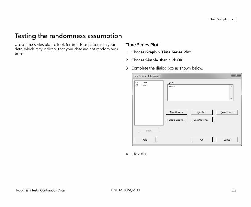
Testing the randomness assumptionUse a time series plot to look for trends or patterns in yourdata, which may indicate that your data are not random overtime.

Time Series Plot1. Choose Graph > Time Series Plot.

2. Choose Simple, then click OK.

3. Complete the dialog box as shown below.

4. Click OK.

Hypothesis Tests: Continuous Data 118

One-Sample t-Test

TRMEM180.SQMEI.1

Interpreting your resultsIf a trend or pattern exists in the data, we would want tounderstand the reasons for them. In this case, the data do notexhibit obvious trends or patterns.

What’s nextCalculate a confidence interval for the true population mean.

Hypothesis Tests: Continuous Data 119

One-Sample t-Test

TRMEM180.SQMEI.1

Confidence intervalsWhat is a confidence intervalA confidence interval is a range of likely values for a populationparameter (such as μ) that is based on sample data. Forexample, with a 95% confidence interval for μ, you can be 95%

Why use a confidence intervalConfidence intervals can help answer many of the same questionsas hypothesis testing:

• Is μ on target?confident that the interval contains μ. In other words, 95 outof 100 intervals will contain μ upon repeated sampling. • How much error exists in an estimate of μ?

• How low or high might μ be?When to use a confidence intervalUse a confidence interval to make inferences about one ormore populations from sample data, or to quantify theprecision of your estimate of a population parameter, such asμ.

For example,

• Is the mean transaction time longer than 30 seconds?

• What is the range of likely values for mean daily revenue?

Hypothesis Tests: Continuous Data 120

One-Sample t-Test

TRMEM180.SQMEI.1

Using the confidence intervalIn the previous analysis, you used a hypothesis test todetermine whether the mean of the mortgage processingtime was different from the target value. You can also use aconfidence interval to evaluate this difference.

1-Sample t1. Choose Stat > Basic Statistics > 1-Sample t.

2. Click Graphs.The Session window results for 1-Sample t include values forthe upper and lower bounds of the 95% confidence interval.Obtain a graphical representation of the interval by selectingIndividual value plot in the Graphs subdialog box.

3. Complete the dialog box as shown below.

4. Click OK in each dialog box.

Hypothesis Tests: Continuous Data 121

One-Sample t-Test

TRMEM180.SQMEI.1

Interpreting your resultsConfidence intervalThe confidence interval is a range of likely values for μ. Minitabdisplays the interval graphically as a blue line on the individualvalue plot.

Under repeated sampling from the same population, theconfidence intervals from about 95% of the samples wouldinclude μ. Thus, for any one sample, you can be 95% confidentthat μ is within the confidence interval.

Note A confidence interval does not represent 95% of the data; this isa common misconception.

Hypothesis Tests: Continuous Data 122

One-Sample t-Test

TRMEM180.SQMEI.1

Interpreting your resultsHypothesis testThe middle tick mark, labeled X, represents the mean of thesample and the red circle, labeled H0, represents thehypothesized population mean (6 hours). You can be 95%confident that the process mean is at least 3.859 hours, andat most 6.298 hours.

Use the confidence interval to test the null hypothesis:

• If H0 is outside the interval, the p-value for the hypothesistest will be less than 0.05. You can reject the null hypothesisat the 0.05 α-level.

• If H0 is inside the interval, the p-value will be greater than0.05. You cannot reject the null hypothesis at the 0.05α-level.

Because H0 falls within the confidence interval, you cannotreject the null hypothesis. Not enough evidence is availableto conclude that μ is different from the target of 6 hours atthe 0.05 significance level.

Hypothesis Tests: Continuous Data 123

One-Sample t-Test

TRMEM180.SQMEI.1

Final considerationsSummary and conclusionsAccording to the t-test and the sample data, you fail to rejectthe null hypothesis at the 0.05 α-level. In other words, thedata do not provide sufficient evidence to conclude the meanprocessing time is significantly different from 6 hours.

The normality test and the time series plot indicate that thedata meet the t-test’s assumptions of normality andrandomness.

The 95% confidence interval indicates the true value of thepopulation mean is between 3.859 hours and 6.298 hours.

Hypothesis Tests: Continuous Data 124

One-Sample t-Test

TRMEM180.SQMEI.1

Final considerationsHypothesesA hypothesis test always starts with two opposing hypotheses.

AssumptionsEach hypothesis test is based on one or more assumptions aboutthe data being analyzed. If these assumptions are not met, theconclusions may not be correct.The null hypothesis (H0):

• Usually states that some property of a population (suchas the mean) is not different from a specified value or froma benchmark.

The assumptions for a one-sample t-test are:

• The sample must be random.

• Sample data must be continuous.• Is assumed to be true until sufficient evidence indicatesthe contrary. • Sample data should be normally distributed (although this

assumption is less critical when the sample size is 30 or more).• Is never proven true; you simply fail to disprove it.

The t-test procedure is fairly robust to violations of the normalityassumption, provided that observations are collected randomlyand the data are continuous, unimodal, and reasonably symmetric(see [1]).

The alternative hypothesis (H1):

• States that the null hypothesis is wrong.

• Can also specify the direction of the difference.Confidence intervalThe confidence interval provides a likely range of values for μ (orother population parameters).

Significance levelChoose the α-level before conducting the test.

• Increasing α increases the chance of detecting a difference,but it also increases the chance of rejecting H0 when it isactually true (a Type I error).

You can conduct a two-tailed hypothesis test (alternativehypothesis of ≠) using a confidence interval. For example, if thetest value is not within a 95% confidence interval, you can rejectH0 at the 0.05 α-level. Likewise, if you construct a 99% confidence

• Decreasing α decreases the chance of making a Type Ierror, but also decreases the chance of correctly detectinga difference.

interval and it does not include the test mean, you can reject H0at the 0.01 α-level.

Hypothesis Tests: Continuous Data 125

One-Sample t-Test

TRMEM180.SQMEI.1