Services Trade Restrictiveness and Manufacturing Productivity:

The Role of Institutions∗

Cosimo Beverelli†† Matteo Fiorini†‡ Bernard Hoekman§

Abstract

We study the effect of services trade restrictiveness on manufacturing productivity for a broad cross-

section of countries at different stages of economic development. Decreasing services trade restric-

tiveness has a positive indirect impact on the manufacturing sectors that use services as intermediate

inputs in production. We identify a critical role of local institutions in shaping this effect: coun-

tries with high institutional capacity benefit the most from services trade policy reforms in terms

of increased productivity in downstream industries. We argue that this reflects the characteristics

of many services and services trade and provide a theoretical framework to formalize our suggested

mechanisms.

Keywords: services trade; institutions; productivity

JEL Classification: F14; F15; F61; F63

∗The opinions expressed in this paper should be attributed to its authors. They are not meant to represent the positionsor opinions of the WTO and its Members and are without prejudice to Members’ rights and obligations under the WTO.Any errors are attributable to the authors. Without implicating them, we thank Andrea Ariu, Mauro Boffa, Ingo Borchert,Antonia Carzaniga, Barbara D’Andrea, Victor Kummritz, Aaditya Mattoo, Andrea Mattozzi, Dominik Menno, SebastienMirodout, Ben Shepherd and participants at the CEPR conference in Modena, the Growth and Development Workshop inRimini, the 4th EU-China trade conference in Florence, the NUPI seminar in Oslo and the 17th ETSG conference in Parisfor useful comments and suggestions. Etienne Michaud provided able research assistance. Cosimo Beverelli and MatteoFiorini thank RECENT and Graziella Bertocchi for the kind hospitality.

†Economic Research Division, World Trade Organization.‡European University Institute. Department of Economics and Robert Schuman Centre for Advanced Studies. E-mail:

Matteo.Fiorini@EUI.eu (corresponding author).§Robert Schuman Centre for Advanced Studies, European University Institute and CEPR.

1 Introduction

Increasing productivity is an essential ingredient of economic growth and development. A large fraction

of such growth originates in the manufacturing sector (Van Ark et al., 2008). The productivity of

manufacturing depends, among others, on the availability of high-quality inputs (Jones, 2011). These

include machinery and intermediate parts and components, as well as a range of services inputs (Johnson,

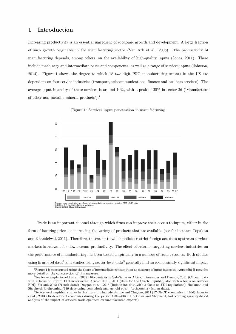
2014). Figure 1 shows the degree to which 18 two-digit ISIC manufacturing sectors in the US are

dependent on four service industries (transport, telecommunications, finance and business services). The

average input intensity of these services is around 10%, with a peak of 25% in sector 26 (‘Manufacture

of other non-metallic mineral products’).1

Figure 1: Services input penetration in manufacturing

0.0

5.1

.15

.2.2

5

15−16 17−19 20 21 22 23 24 25 26 27 28 29 30 31 32 33 34 35 36−37

Services input penetration are shares of intermediate consumption from the 2005 US IO tableISIC Rev. 3 2−digit manufactuing industriesSource: OECD STAN IO Database

Transports Telecom Finance Business

Trade is an important channel through which firms can improve their access to inputs, either in the

form of lowering prices or increasing the variety of products that are available (see for instance Topalova

and Khandelwal, 2011). Therefore, the extent to which policies restrict foreign access to upstream services

markets is relevant for downstream productivity. The effect of reforms targetting services industries on

the performance of manufacturing has been tested empirically in a number of recent studies. Both studies

using firm-level data2 and studies using sector-level data3 generally find an economically significant impact

1Figure 1 is constructed using the share of intermediate consumption as measure of input intensity. Appendix B providesmore detail on the construction of this measure.

2See for example Arnold et al., 2008 (10 countries in Sub-Saharan Africa); Fernandes and Paunov, 2011 (Chilean datawith a focus on inward FDI in services); Arnold et al., 2011 (data for the Czech Republic, also with a focus on servicesFDI); Forlani, 2012 (French data); Duggan et al., 2013 (Indonesian data with a focus on FDI regulations); Hoekman andShepherd, forthcoming (119 developing countries); and Arnold et al., forthcoming (Indian data).

3Sector-level empirical studies in this literature include Barone and Cingano, 2011 (17 OECD economies in 1996); Bourleset al., 2013 (15 developed economies during the period 1984-2007); Hoekman and Shepherd, forthcoming (gravity-basedanalysis of the impact of services trade openness on manufactured exports).

1

of services productivity (or firms’ access to services) on productivity in manufacturing.4

While this literature has established the importance of the indirect linkage between services trade

policy and economic performance of industries that are downstream in the relevant supply chain, less has

been done to account for the specific characteristics of services production and exchange in shaping this

causal relationship. The main contribution of this paper is to identify the role that economic institutions

play as a determinant of the size of this indirect effect. Specifically, we estimate the impact of services

trade restrictiveness on manufacturing productivity and demonstrate that the quality of institutions

shapes the relationship between upstream services openness and downstream manufacturing productivity.

We argue that this is a reflection of the characteristics of services and services trade, which often require

a foreign firm to invest or otherwise establish a physical presence in an importing market to sell services.

To provide a conceptual framework for our empirical findings, we also develop a simple theoretical model.

This embodies key characteristics of services and services trade and identifies why one should expect the

observed moderating effect of institutions.

The paper is organised as follows. Section 2 motivates the analysis and briefly relates our approach

to some of the literature. Section 3 turns to the econometric exercise, and presents the database, the

specifications and the estimation results. In section 4 we develop a simple theoretical framework to

rationalise the empirical finding that institutional capacity is a determinant of the magnitude of the

positive effect of services trade openness on productivity in downstream industries. Section 5 concludes.

2 Motivation and Related Literature

Economic institutions and associated measures of the quality of economic governance such as control

of corruption, rule of law, regulatory quality, contract enforcement, and more generally the investment

and business climate are crucial determinants of economic development.5 In the services literature, some

studies introduce institutional quality as a determinant of the services trade policy stance (van der Marel,

2014a) and of the coverage of services policy commitments made in trade agreements (van der Marel and

Miroudot, 2014). Building on the literature that identifies institutions as a trigger for comparative ad-

vantage in industries that are more sensitive to the institutional environment (notably complex industries

with contract-intensive production processes)6, van der Marel (2014b) argues that the ability of countries

to provide complementary domestic regulatory policies accompanying services liberalization is a source

4Of course, the link between upstream and downstream performance is not limited to services. Blonigen (forthcoming) isa recent cross-country analysis of the impact of upstream policies in a non-services sector (the steel industry) on downstreameconomic outcomes.

5See, among others, Acemoglu et al. (2001; 2005) and Rodrik et al. (2004). In the trade literature, a number of studieshave looked at institutions as determinants of bilateral trade flows as well as offshoring and FDI decisions at the firm level.Anderson and Marcouiller (2002) build a gravity framework where imports depend on the institutional settings affectingthe security of trade and show that weak institutions limit trade as much as tariffs do. Other topics in the institutionsand trade literature are the effect of trade outcomes and policies on (endogenous) institutions and the role of informalinstitutions as social capital and trust. For a general review of the literature we address the reader to WTO (2013).

6See Nunn (2007); Levchenko (2007); Costinot (2009).

2

of comparative advantage in downstream goods trade.

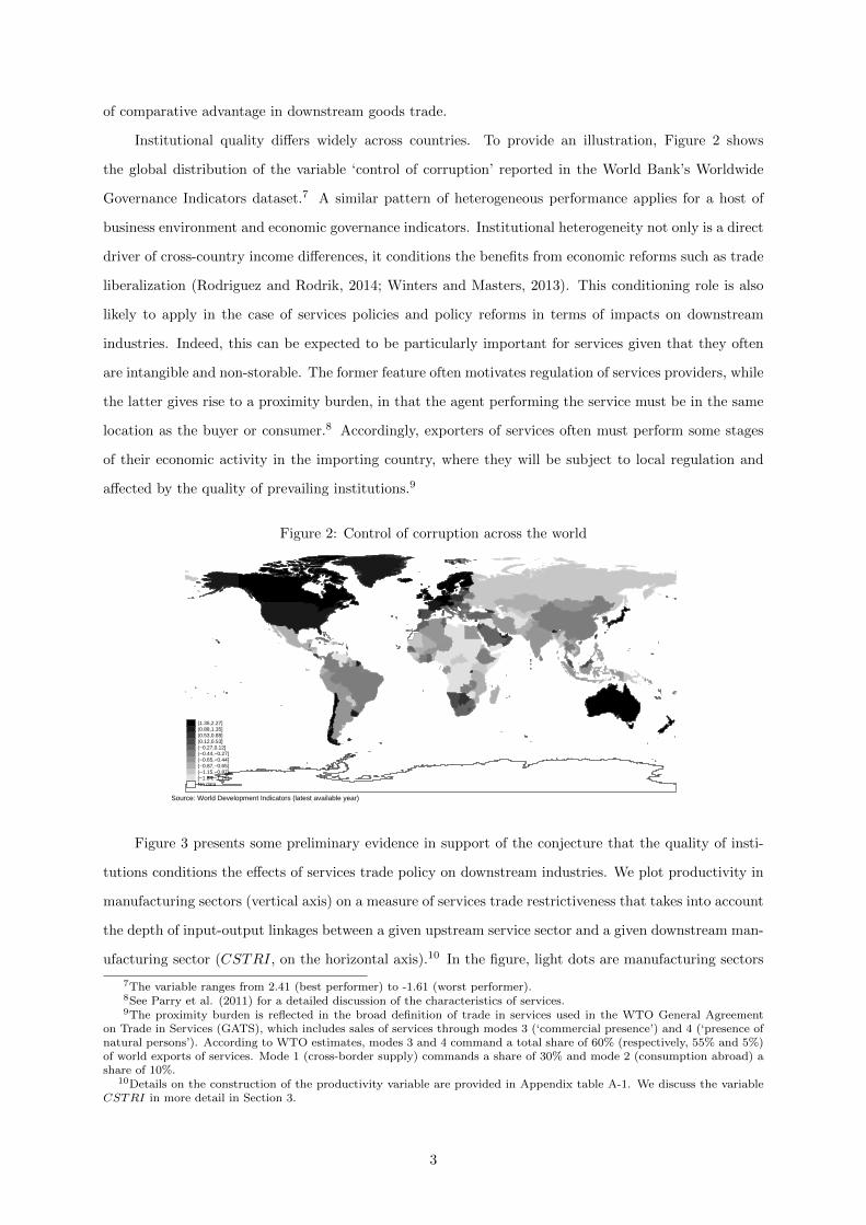
Institutional quality differs widely across countries. To provide an illustration, Figure 2 shows

the global distribution of the variable ‘control of corruption’ reported in the World Bank’s Worldwide

Governance Indicators dataset.7 A similar pattern of heterogeneous performance applies for a host of

business environment and economic governance indicators. Institutional heterogeneity not only is a direct

driver of cross-country income differences, it conditions the benefits from economic reforms such as trade

liberalization (Rodriguez and Rodrik, 2014; Winters and Masters, 2013). This conditioning role is also

likely to apply in the case of services policies and policy reforms in terms of impacts on downstream

industries. Indeed, this can be expected to be particularly important for services given that they often

are intangible and non-storable. The former feature often motivates regulation of services providers, while

the latter gives rise to a proximity burden, in that the agent performing the service must be in the same

location as the buyer or consumer.8 Accordingly, exporters of services often must perform some stages

of their economic activity in the importing country, where they will be subject to local regulation and

affected by the quality of prevailing institutions.9

Figure 2: Control of corruption across the world

(1.35,2.27](0.88,1.35](0.53,0.88](0.12,0.53](−0.27,0.12](−0.44,−0.27](−0.65,−0.44](−0.87,−0.65](−1.15,−0.87][−1.84,−1.15]No data

Source: World Development Indicators (latest available year)

Figure 3 presents some preliminary evidence in support of the conjecture that the quality of insti-

tutions conditions the effects of services trade policy on downstream industries. We plot productivity in

manufacturing sectors (vertical axis) on a measure of services trade restrictiveness that takes into account

the depth of input-output linkages between a given upstream service sector and a given downstream man-

ufacturing sector (CSTRI, on the horizontal axis).10 In the figure, light dots are manufacturing sectors

7The variable ranges from 2.41 (best performer) to -1.61 (worst performer).8See Parry et al. (2011) for a detailed discussion of the characteristics of services.9The proximity burden is reflected in the broad definition of trade in services used in the WTO General Agreement

on Trade in Services (GATS), which includes sales of services through modes 3 (‘commercial presence’) and 4 (‘presence ofnatural persons’). According to WTO estimates, modes 3 and 4 command a total share of 60% (respectively, 55% and 5%)of world exports of services. Mode 1 (cross-border supply) commands a share of 30% and mode 2 (consumption abroad) ashare of 10%.

10Details on the construction of the productivity variable are provided in Appendix table A-1. We discuss the variableCSTRI in more detail in Section 3.

3

in countries lying above the sample median of the variable control of corruption (the main proxy for

institutional quality in the empirical analysis); dark dots are manufacturing sectors in countries lying

below this sample median. In the case of countries with high institutional quality, the (solid) regression

line is negatively sloped, with a statistically significant coefficient of -0.112. Conversely, for countries

with low institutional quality the slope of the (dashed) regression line is not statistically different from

zero. These data suggest that institutional quality is a determinant of the potential gains from services

trade liberalization.

Figure 3: CSTRI and manufacturing productivity across institutional regimes: descriptive evidence

810

1214

16Lo

g of

labo

r pr

oduc

tivity

(Y

/L)

0 5 10 15CSTRI

High control of corruption (CC) Linear fit if High CCLow control of corruption (CC) Linear fit if Low CC

Coeff. if High CC = −0.112 (s.e. = 0.020)Coeff. if High CC = 0.027 (s.e. = 0.021)

We can think of two broad mechanisms through which institutions may condition the downstream

effects of upstream services trade policy, given a presumption that foreign firms must establish some

degree of commercial presence in an importing country to contest the market. First, for a given level

of trade restrictiveness implied by policy, the institutional environment in a country may affect entry

decisions of potential foreign suppliers, giving rise to a selection or ex-ante effect of institutions.11 To

illustrate this channel, consider a global provider of telecommunication services, Vodafone. This firm has

a direct presence in 21 ‘local’ markets, and an indirect presence in 55 ‘partner’ markets.12 Of these 76

markets, 19 (25%) are in countries with relatively low institutional quality (measured by the control of

corruption variable being less than the sample median) while the other 57 (75%) are in countries with

relatively high institutional quality (control of corruption above the sample median). If we consider the

11Theoretical models of multinational firms decisions in an international framework with country-level differences incontract enforcement institutions are developed in Antras and Helpman (2004) and Grossman and Helpman (2005). Bernardet al. (2010) find that better governance in the destination countries is associated with a higher number of affiliatesestablished by foreign multinationals. However, such a relationship is not found to be robust in Blonigen and Piger (2014).

12Vodafone data have been collected by the authors from the official Vodafone web page: http://www.vodafone.com/

content/index/about/about-us/where.html.

4

markets where Vodafone is not present, either directly or in partnership with a local provider, 87 out of

142 (61%) are in countries with relatively low institutional quality and 55 (38%) are in countries with

relatively high institutional quality.13 Regression analysis suggests that even after controlling for country

size (level of GDP) and for the level of services trade restrictiveness in telecommunications, institutional

quality has a positive and statistically significant effect on the probability of Vodafone entering a market

by establishing a direct or indirect commercial presence.14

Second, conditional on entry, the quality of the exporters’ output may depend on the institutional

environment of the country where demand is located and the service is performed. A number of recent

studies linking firm productivity with the institutional environment in which firms operate confirm this

hypothesis.15

Our empirical analysis differs from existing country-sector studies on the link between upstream

restrictions and downstream manufacturing productivity in several respects. Papers such as Barone and

Cingano (2011) and Bourles et al. (2013) focus on OECD countries, a relatively homogenous group

of mostly rich economies. Our sample of countries spans 27 nations classified as ‘high income’ by the

World Bank, 16 upper middle income countries, 10 lower middle income countries and 4 low income

economies. This allows to meaningfully test for heterogeneous effects across countries with very different

institutional capacity. Moreover, both papers cited above measure services restrictions using the OECD

Product Market Regulation (PMR) indicator for non-manufacturing industries. This variable has a strong

focus on domestic policies and therefore does not capture the important dimensions of services trade

outlined above. Using the World Bank Services Trade Restrictiveness index, Hoekman and Shepherd

(forthcoming) focus only on developing countries. Their gravity analysis of the effect of services trade

openness on manufacturing exports does not take into account input-output linkages between services

and manufacturing.

This paper complements van der Marel (2014b), who investigates whether countries with a high

level of regulatory capacity are better able to export in goods produced in industries that make relatively

intensive use of services. While van der Marel uses a world-average STRI for each service sector (as the

sector-level component of the country-sector interaction term representing regulatory capacity, in line

with the methodology proposed by Chor, 2010), we use country-level STRI measures to identify and

quantify the causal impact of services trade reforms on downstream productivity.

13A test of equality of means rejects the null hypothesis that the probability of Vodafone’s commercial presence is thesame in the two groups of countries with low and high institutional quality (106 countries each), in favour of the alternativehypothesis that such probability is higher in the group of countries with high institutional quality.

14Regression results are available from the authors on request.15See for example Gaviria (2002), Dollar et al. (2005), Lensink and Meesters (2014) and Borghi et al. (forthcoming).

5

3 Empirics

3.1 Empirical model and identification strategy

The objective of the empirical analysis is to estimate the impact of service trade restrictiveness on

productivity in downstream manufacturing industries, and how institutional quality affects such impact.

We follow the approach pioneered by Rajan and Zingales (1998), assuming that the effect of up-

stream services trade policy on downstream productivity is a positive function of the intensity of services

use as intermediate inputs into downstream sectors. Therefore, the regressor of interest is constructed by

interacting a country-sector measure of trade restrictiveness in services with a measure of services input

use by downstream industries derived from input-output data. Formally, for any country i and down-

stream manufacturing sector j, we define a composite services trade restrictiveness indicator (CSTRI)

as follows:

CSTRIij =∑s

STRIis ×wijs (3.1)

where STRIis is the level of services trade restrictiveness for country i and services sector s and wijs is a

measure of input penetration of service s into manufacturing sector j of country i. We use for w the shares

of total intermediate consumption: wijs is the share associated to sector s in the total consumption of

intermediate inputs (both domestically produced and imported) of sector j in country i.16 The baseline

productivity regression is then:

yij = α + βCSTRIij + γ′xij + δi + δj + εij (3.2)

where the dependent variable is a measure of productivity of downstream manufacturing sector j in

country i; δi and δj are respectively country and downstream sector individual effects; and xij is the

column vector of relevant regressors varying at the country-sector level. In the baseline regressions, this

vector contains the variable Tariff, the logarithm of the effectively applied tariff by country i in sector

j. In subsequent robustness checks, we add the variable Tariff, the logarithm of the weighted average of

tariffs effectively applied in manufacturing sectors k ≠ j (see Section 3.4 for a details on the construction

of this variable).

The coefficient β in model 3.2 is expected to be negative. A potential mechanism is the following.

Consider a decrease in the variable CSTRI as an inflow of a factor of production, services, from abroad.

The Rybczinski theorem suggests that additional services will be absorbed by service-intensive indus-

tries, which will expand, attracting other factors of production (including domestic services) from less

service-intensive industries. These industries will in turn contract, releasing factors of production to the

expanding ones. At the same time, the average quality of services increases with services trade liberaliza-

16For the derivation of the shares of intermediate consumption from the IO tables, see Appendix B.

6

tion. Even keeping the factor input mix constant, therefore, the productivity of labor in service-intensive

(expanding) industries will increase, because each worker will be endowed with the same amount of better-

performing services than before the liberalization.17 The productivity of labor in less service-intensive

(contracting) industries should in turn not be affected, as they do not absorb more productive services. In

other words, in these industries each worker will be endowed with the same amount of equally-performing

services as before the liberalization. Since β represents the average effect across expanding industries –

where y should be negatively associated with CSTRI – and contracting industries – where the association

should be null – β is expected to be negative.

Following the introductory discussion on the role of institutional variables in moderating the effect

of services trade restrictiveness on downstream productivity, we allow for heterogeneous effects of the

regressor of interest (CSTRI) across country-level institutional capacity. Accordingly, we propose the

following interaction model:

yij = α + βCSTRIij + κ(CSTRIij × ICi) + γ′xij + δi + δj + εij (3.3)

where ICi is a continuous proxy for institutional capacity in country i.18 In this second specification,

the impact of service trade restrictiveness is given by β + κICi and therefore varies at the country level

depending on the institutional framework. In line with the theoretical mechanisms outlined in Section

1 and formalized in Section 4, the coefficient k should be negative (the negative effect of CSTRI on y

should be larger in countries with high institutional capacity).

We now discuss several identification issues which are common to the two specifications (3.2) and

(3.3).

3.1.1 Omitted variables bias

All regressions are estimated including country fixed effects and sector dummies. This neutralizes the risk

of estimation bias coming from omitted variables varying at the country or sectoral level. What remains

is the variability at the country-sector level. In particular we need to control for those variables that,

varying at the country-sector level, are potential determinants of productivity and that can be correlated

with services trade restrictiveness. The most relevant candidate is a measure of restrictiveness for trade

in goods (imports). Accordingly, we always include, as control, the tariff variable(s) described above.

3.1.2 Endogeneity of the input penetration measure

The intensity of services consumption by a downstream manufacturing sector may be affected by the

degree of services trade restrictiveness (less restricted services trade enhancing downstream intermediate

17The same reasoning would also apply to total factor productivity, TFP, because higher-quality services would raise theproductivity of all other factors.

18We do not include the main effect of ICi in equation (3.3) as it is accounted for by the country specific effects.

7

consumption) and the productivity in the manufacturing sector itself (more productive manufacturing

sectors being able to consume more differentiated services). In the first case the number of manufacturing

industries for which the ‘treatment’ (lower trade restrictiveness in the services sector) is likely to have

more bite would be increasing with the treatment itself. In the second case we would have an issue of

reverse causality. Killing two birds with one stone, we measure wijs of any country i with the input

penetration of service s into industry j for country c ≠ i. We follow here the assumption widely adopted

in the literature originating from Rajan and Zingales (1998), taking the United States’ input-output

coefficients as representative of the technological relationships between industries. We therefore set c =

US and remove the US from the sample.

3.1.3 Endogeneity of the services trade restrictiveness measure

Downstream productivity – or lack thereof – could affect the degree of trade liberalization for upstream

industries through lobbying, generating a problem of reverse causation. If low productivity industries

downstream are the ones lobbying for deeper upstream liberalization, our results would have to be in-

terpreted – at worst – as a lower bound for the impact of services trade openness on manufacturing

productivity, conditional on downstream lobbying (this argument is discussed in Bourles et al., 2013).

To account for this and for the more critical case where high productivity manufacturing industries

are the ones with the right incentives and capabilities to exert effective lobbying pressure for services

trade openness19, we propose an instrument for services trade restrictiveness. Section 3.3.1 discusses the

construction of the instrument and the results of IV regressions.

3.2 Data

Given the focus on the role of institutions in shaping the indirect effect of services trade policy, data

comprising the maximum variability in country level institutional capacity is needed. The World Bank’s

Services Trade Restrictiveness Database (STRD) offers a unique country coverage (103 economies) for

services trade policies affecting imports. These include measures on market access; national treatment

provisions; and domestic regulation that have a clear impact on trade. The Services Trade Restrictiveness

Indexes cover five services sectors – financial services (banking and insurance), telecommunications, retail

distribution, transportation and professional services (accounting and legal) – and the most relevant

modes of supplying the respective service. These are commercial presence or FDI (mode 3) in every sub-

sector; in addition, cross-border supply (mode 1) of financial, transportation and professional services;

and the presence of service supplying individuals (mode 4) only for professional services (see Borchert et

al., 2012 for a detailed description of the database). In the empirical analysis, we alternatively use the

STRI aggregated across all available modes or the mode 3 STRI. Since we consider the role of importing

19The latter case is more critical because it would imply an upward bias in the estimated coefficients.

8

countries’ institutions, the absence of information on mode 2 (consumption abroad) in the STRI data is

harmless. STRI data does not vary over time. It captures the prevailing policy regimes in the mid-2000s.

Data on input penetration comes from the mid-2000s OECD STAN IO Tables, where sectors are

mapped to the ISIC Rev. 3 classification and aggregated at the 2 digits level. Productivity measures are

constructed using data from the UNIDO Industrial Statistics Database. The data varies across countries,

years and manufacturing sectors (ISIC Rev. 3). The key feature of the UNIDO database is that it

provides the widest country coverage with respect to possible alternative sources, such as EU KLEMS or

OECD STAN.20 Following Hoekman and Shepherd (forthcoming), we use labor productivity as a proxy

for industry productivity.21

Data on institutional capacity is from the World Bank’s Worldwide Governance Indicators. Tariff

data is from UNCTAD TRAINS.

The estimation sample includes 57 countries and 18 manufacturing sectors (listed in Appendix table

A-2). A description of all the variables used in the estimations, including the data sources, is in Appendix

table A-1. Descriptive statistics are in Table 1.

Table 1: Summary statistics

Variable mean median sd min max

Productivity 11.76 11.72 1.36 7.23 16.26CSTRI 4.35 3.61 2.92 0.00 22.62IC 2.92 2.73 1.01 1.26 5.03Tariff 0.85 0.92 0.38 0.00 1.61

Tariff 0.88 0.95 0.31 0.23 1.54

From estimation sample of column (8) of Table 8

IC = control of corruption

3.3 Results

The main estimation results for the baseline specification (3.2) and the interaction model (3.3) are given

in Table 2. The first two columns use the STRI measure aggregated across all modes of supply, while the

last two columns focus on measures relevant only for trade through commercial presence (Mode 3).

The estimated coefficient of the composite measure of services trade restrictiveness has the expected

negative sign in the baseline specification for both All modes in column (1) and Mode 3 in column (3): less

restrictive policy environments are associated with higher productivity in downstream manufacturing. In

the first case, however, the estimate is not statistically different from 0, while in the second case (mode 3)

it is only weakly statistically significant (0.1 level). Moving to the interaction model, we find a statistically

20The EU KLEMS database covers Australia, Japan, the US and 25 UE countries (O’Mahony and Timmer, 2009). TheOECD STAN database covers 33 OECD countries.

21To the best of our knowledge there exists no dataset providing more refined measures of industry productivity, such asTFP, for a large and heterogeneous cross-section of countries. Therefore we are bound to rely on labor productivity. Thisis common to other studies where the research interest lies in wide country coverage (see for instance Rodrik, 2013).

9

Table 2: Baseline and Interaction Model Estimation

All modes Mode 3

(1) (2) (3) (4)

CSTRI -0.025 0.065 -0.038* 0.052(0.024) (0.038) (0.021) (0.032)

CSTRI × IC -0.041*** -0.039***(0.014) (0.012)

Tariff -0.120 -0.110 -0.323* -0.304(0.084) (0.083) (0.186) (0.185)

Observations 912 912 912 912R-squared 0.522 0.526 0.524 0.528

Robust (country-clustered) standard errors in parentheses

* p<0.10, ** p<0.05, *** p<0.01

Country fixed effects and sector dummies always included

IC = control of corruption

significant, negative coefficient for the interaction term. Lower services trade restrictiveness is associated

with higher downstream manufacturing productivity, with the estimated effect increasing with country-

level institutional capacity. The results of the interaction model suggest that the weak or no significance

at the baseline specification level is driven by a composition effect. The role of institutions based on the

estimation of the Mode 3 case is further illustrated in Figure 4.22

Figure 4: Impact of use unit increase in CSTRI (Mode 3) on the downstream log productivity y

−.3

−.2

−.1

0.1

Effe

ct o

n lo

g pr

oduc

tivity

1.00 2.00 3.00 4.00 5.00

Control of Corruption in year 2007

Estimated Impact 95% CI Mean Moderator

For approximately 95% of our sample the effect of CSTRI has the expected negative sign and,

22The figure reports marginal effects evaluated at 39 values of the control of corruption variable and 95% confidenceintervals. The latter are calculated using the Delta method.

10

for approximately 60% of the observations (those with a level of control of corruption higher that 2.5),

the effect is statistically significant at the 0.05 level. The positive effect of lower trade restrictiveness

in upstream services sectors increases with institutional capacity. The effect is not statistically different

from zero for low levels of institutional capacity (approximately 40% of our sample).

To get a sense of the economic relevance of this result consider the following quantification exercise.

Take four countries with similar mean values of the composite measure of services trade restrictiveness

CSTRI for Mode 3: Austria, Canada, Italy and Tanzania. These countries have very different institu-

tional capacities or performance. Austria and Canada rank respectively 6th and 7th in terms of control

of corruption in the sample, while Italy ranks 25th and Tanzania 43rd. Assuming that the four economies

adopt the less restrictive services trade regime observed in the UK23, productivity in downstream man-

ufacturing increases by 18.2% in Austria, 16.7% in Canada, 7.3% in Italy and only 3.9% in Tanzania.

Finally, the coefficient on Tariff is negative, although not statistically significant, indicating that

more protected sectors are also the least productive ones.24

3.3.1 Instrumenting for the services trade restrictiveness measure

As noted above, there are reasons one might be concerned with endogeneity of the STRI measures. In

the spirit of Arnold et al. (2011; forthcoming), we instrument for STRIi using the weighted average of

STRI in other countries c ≠ i:

STRIIVis ≡∑c

STRIcs × SIci (3.4)

where SIic ≡ 1 − {pcGDPi

pcGDPi+pcGDPc}

2− {

pcGDPc

pcGDPi+pcGDPc}

2is a similarity index in GDP per capita between

the two countries i and c.25 Such weights should reflect similar trade policy motives, assuring the

relevance of the instrument. Moreover, to satisfy the exclusion restriction, the c countries are taken

from geographical regions different from that of country i. This minimises the potential linkages between

services trade regimes in the c countries and the lobbying activity of i’s manufacturing sector (see section

3.1.3).26

The results are presented in Table 3. The instrument passes the standard tests. The results are,

however, quantitatively very similar to the baseline results of Table 2, suggesting we do not need to be

concerned with endogeneity of the services trade restrictiveness measure.

23Such a shift entails a reduction in the CSTRI by approximately 45% of a sample standard deviation for each of the 4selected countries.

24We make no attempt to claim a causal link between tariff protection and sectoral productivity, as this would be beyondthe scope of this paper.

25We take the definition of the similarity index from Helpman (1987).26We thank Ben Shepherd for suggesting using countries c from different regions than i, rather than the same region as

i.

11

Table 3: Instrumental variable regressions

All modes Mode 3

(1) (2) (3) (4)

CSTRI -0.124* 0.028 -0.027 0.048(0.072) (0.061) (0.052) (0.058)

CSTRI × IC -0.053*** -0.044***(0.019) (0.017)

Tariff -0.114 -0.103 -0.120 -0.109(0.075) (0.073) (0.075) (0.073)

Observations 912 912 912 912R-squared 0.515 0.523 0.522 0.526First-stage F statisticsCSTRI 44.56 55.17 68.59 34.53(p-value) 0.00 0.00 0.00 0.00CSTRI × IC 39.13 46.68(p-value) 0.00 0.00

Underid SW Chi-sq statisticsCSTRI 45.58 219.92 70.15 145.24(p-value) 0.00 0.00 0.00 0.00CSTRI × IC 186.81 244.07(p-value) 0.00 0.00

Weak id SW F statisticsCSTRI 44.56 214.78 68.59 141.85CSTRI × IC 182.44 238.36

Stock-Wright LM S statisticsChi-sq 3.87 9.01 0.33 8.21(p-value) 0.049 0.011 0.566 0.016

Robust (country-clustered) standard errors in parentheses

* p<0.10, ** p<0.05, *** p<0.01

Country fixed effects and sector dummies always included

“SW” refers to Sanderson and Windmeijer (forthcoming)

Instrument for CSTRIi: weighted average of CSTRIk (see Section 3.1.3)

IC = control of corruption

3.3.2 Random services trade restrictiveness

To ensure that our results can be given a clear economic interpretation, we perform a Placebo experiment

in which the ‘treatment’ (services trade restrictiveness), rather than being constructed from real data, is

randomly assigned. We construct the variable CSTRIij = ∑s STRIis ×wijs, where STRIis is a random

draw from a uniform distribution with support [0,100]. We then perform 100,000 regressions of model

(3.3), each with a different, randomly constructed CSTRIij , and we estimate the marginal effects. As

in the baseline case, we evaluate the marginal effects at 39 values of the control of corruption variable.

The resulting dataset, therefore, contains 3,900,000 estimated marginal effects. Out of those, 83% are

not statistically different from zero.

Figure 5 graphically represents the marginal effects with the confidence intervals – averaged across all

the 100,000 regressions. It is apparent that the marginal effects are never statistically different from zero.

12

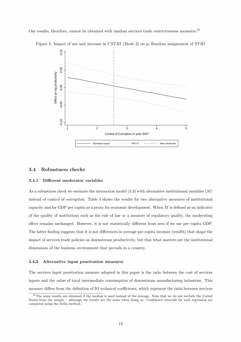
Our results, therefore, cannot be obtained with random services trade restrictiveness measures.27

Figure 5: Impact of use unit increase in CSTRI (Mode 3) on y: Random assignement of STRI

−0.

10−

0.05

0.00

0.05

0.10

Effe

ct o

n lo

g pr

oduc

tivity

1 2 3 4 5

Control of Corruption in year 2007

Estimated Impact 95% CI Mean Moderator

3.4 Robustness checks

3.4.1 Different moderator variables

As a robustness check we estimate the interaction model (3.3) with alternative institutional variables (M)

instead of control of corruption. Table 4 shows the results for two alternative measures of institutional

capacity and for GDP per capita as a proxy for economic development. When M is defined as an indicator

of the quality of institutions such as the rule of law or a measure of regulatory quality, the moderating

effect remains unchanged. However, it is not statistically different from zero if we use per capita GDP.

The latter finding suggests that it is not differences in average per capita incomes (wealth) that shape the

impact of services trade policies on downstream productivity, but that what matters are the institutional

dimensions of the business environment that prevails in a country.

3.4.2 Alternative input penetration measures

The services input penetration measure adopted in this paper is the ratio between the cost of services

inputs and the value of total intermediate consumption of downstream manufacturing industries. This

measure differs from the definition of IO technical coefficients, which represent the ratio between services

27The same results are obtained if the median is used instead of the average. Note that we do not exclude the UnitedStates from the sample – although the results are the same when doing so. Confidence intervals for each regression arecomputed using the Delta method.

13

Table 4: Interaction model estimation with alternative moderator variables

Moderator (M) Rule of Law Reg. Quality GDP per capita

All Modes Mode 3 All Modes Mode 3 All Modes Mode 3

(1) (2) (3) (4) (5) (6)

CSTRI -0.032 -0.039* -0.034 -0.040* -0.015 -0.027(0.024) (0.021) (0.025) (0.021) (0.024) (0.020)

CSTRI ×M -0.046*** -0.046*** -0.044*** -0.045*** -0.000 -0.000(0.014) (0.012) (0.014) (0.012) (0.000) (0.000)

Tariff -0.532* -1.498** -0.303 -1.252** -0.800** -1.826**(0.287) (0.733) (0.184) (0.619) (0.399) (0.860)

Observations 912 912 912 912 912 912R-squared 0.527 0.530 0.525 0.529 0.525 0.526

Robust (country-clustered) standard errors in parentheses

* p<0.10, ** p<0.05, *** p<0.01

Country fixed effects and sector dummies always included

inputs and total output of a downstream sector.28 Our definition does not embed differences in value

added across manufacturing sectors, representing therefore a better proxy for technological differences in

intermediate input consumption. To test the robustness of our preferred measure of input penetration,

we replicate the estimation using both US technical coefficients and the coefficients derived from the

US Leontief inverse matrix, which captures also the indirect linkages between upstream and downstream

industries.29 Estimation results are given in Table 5.

Table 5: Estimation with Technical and Leontief IO coefficients

IO weights Technical Leontief

All modes Mode 3 All modes Mode 3

(1) (2) (3) (4) (5) (6) (7) (8)

CSTRI -0.068 0.131 -0.087** 0.111 -0.080 0.172 -0.103 0.176(0.052) (0.081) (0.043) (0.075) (0.082) (0.133) (0.062) (0.144)

CSTRI × IC -0.093*** -0.085*** -0.116*** -0.119**(0.027) (0.026) (0.042) (0.049)

Tariff -0.122 -0.085 -0.330* -0.260 -0.126 -0.078 -0.344* -0.241(0.084) (0.084) (0.186) (0.186) (0.085) (0.087) (0.187) (0.197)

Observations 912 912 912 912 912 912 912 912R-squared 0.523 0.529 0.525 0.531 0.522 0.527 0.525 0.529

Robust (country-clustered) standard errors in parentheses

* p<0.10, ** p<0.05, *** p<0.01

Country fixed effects and sector dummies always included

IC = control of corruption

28The ratio between the cost of services inputs and the value of the downstream industry output is the proxy for directinput penetration usually adopted in the empirical literature on the indirect effect of services policies on manufacturing (seefor example Barone and Cingano, 2011).

29For a derivation of those alternative input penetration measures from the IO Table, see Appendix B.

14

The sign and statistical significance of the estimated coefficients is robust across all measures of

input penetration. Given the smaller size of technical and Leontief IO weights with respect to the shares

of total intermediate consumption, the higher coefficient estimates in Table 5 generate economic effects

that are similar in magnitude.

Given the heterogeneity of the countries in our sample, one can question the representativeness of

the US as the baseline country for the IO linkages. In Table 6 we present results using the services shares

of manufacturing intermediate consumption derived from China’s 2005 IO accounting matrix. China was

classified as lower middle income country by the World Bank in 2006.30 Therefore it represents a more

representative baseline for our estimation sample which includes both middle and low income countries.

The sign and statistical significance of the coefficient estimates are not affected by the use of China’s

data. The higher values of the coefficients using Chinese IO data suggests that the use of US data is a

conservative choice for the economic quantification of the results.

Table 6: Estimation with Chinese input penetration measures

All modes Mode 3

(1) (2) (3) (4)

CSTRI -0.081 0.135 -0.099** 0.083(0.050) (0.090) (0.043) (0.083)

CSTRI × IC -0.094*** -0.078**(0.032) (0.030)

Tariff -0.085 -0.084 -0.277 -0.270(0.086) (0.084) (0.188) (0.187)

Observations 912 912 912 912R-squared 0.526 0.529 0.528 0.531

Robust (country-clustered) standard errors in parentheses

* p<0.10, ** p<0.05, *** p<0.01

Country fixed effects and sector dummies always included

China excluded from the estimation sample

IC = control of corruption

Barone and Cingano (2011) argue that country-specific measures of input intensity carry an id-

iosyncratic component which is likely to be related to the trade restrictiveness regime. In that case the

sign of the estimation bias would be ambiguous, requiring a robustness check which does not rely on

country-specific weights (Ciccone and Papaioannou, 2006). We follow the approach adopted by Barone

and Cingano (2011) and instrument the US shares of services s in total intermediate consumption with:

wIVjs ≡ δj + γjSTRIcs ∀s (3.5)

where δj and γj are estimates from the following sector s-specific regression in which country c has been

30In 2006 China had a per capita GNI (Atlas method) of 2,050 US dollars. For that year the GNI per capita interval forlower middle income countries was fixed by the World Bank at 906-3,595 US dollars.

15

excluded from the sample:31

wijs = δi + δj + γjSTRIis + εij ∀s (3.6)

The input intensity measures derived in (3.6) minimise by construction the idiosyncratic component

present in any country-specific proxy. Consistently with the literature, we chose country c to be equal

to the US.32 We also perform this IV exercise by setting c equal to Sweden, the country with the lowest

average STRI values across services sectors (both for Mode 3 and for All modes) of the countries in the

sample used for equations (3.6).33 The results are presented in Table 7.

Although the statistical significance of the estimated coefficients is reduced (especially in the case

where c is set equal to Sweden), their signs and magnitudes are in line with the baseline results.

Finally, to show how important input-output relationships between upstream services and down-

stream manufacturing are, we have performed a counterfactual Placebo analysis with randomly gener-

ated input penetration coefficients. The procedure is similar to the one adopted by Keller (1998). In a

regression in which a country’s R&D is affected by a weighted average of foreign countries’ R&D – with

weights given by bilateral import shares – the author replaces bilateral import shares from trade data with

random shares, drawn from a uniform distribution with support [0,1]. Likewise, we create the variable

CSTRIij = ∑s STRIis × wijs, where wijs are random draws from a uniform distribution with support

[0,100]. As in Section 3.3.2, we perform 100,000 regressions and estimate 3,900,000 marginal effects,

with a 95% confidence interval. Out of the estimated marginal effects, 79% are not statistically different

from zero. Marginal effects with the confidence intervals – averaged across all the 100,000 regressions –

are presented in Figure 6. They are never statistically different from zero. Our results, therefore, cannot

be obtained with random input penetration measures.

3.4.3 Additional tariff controls

Import protection for other manufacturing sectors k ≠ j should also matter – as shown, among others, by

Goldberg et al. (2010). To control for this, we augment model (3.3) with the variable Tariff, constructed

as:

Tariff =∑k

τik ×wjk (3.7)

31This methodology was introduced by Ciccone and Papaioannou (2006) to instrument US industry capital growth. Ourestimates are obtained accounting for the fact that the dependent variable in (3.6) is fractional, applying the specificationsuggested in Papke and Wooldridge (1996).

32A rationale for this is that the US is one of the least regulated countries in a historical perspective (Barone and Cingano,2011).

33Estimation of the models (3.6) requires country specific input intensity measures (wijs) and services trade restrictivenessmeasures (STRIis). The sample size therefore is determined by the intersection of the country coverage of the OECD STANIO Database and that of the World Bank STR Database. This intersection includes 32 countries: Australia, Austria, Brazil,Bulgaria, Canada, Chile, China, Czech Republic, Denmark, Finland, France, Germany, Greece, Hungary, India, Indonesia,Ireland, Italy, Japan, South Korea, Lithuania, Mexico, Netherlands, Poland, Portugal, Romania, South Africa, Spain,Sweden, Turkey, United Kingdom and United States. This limited intersection in the country coverage of the two databasesdoes not allow to perform a robustness check that makes use of the shares of intermediate consumption specific to eachcountry (the baseline estimation sample counts 57 countries plus the US). In any event, the endogeneity issues associatedwith country-specific input intensity measures would have made this particular robustness check quite problematic (seeSection 3.1.2).

16

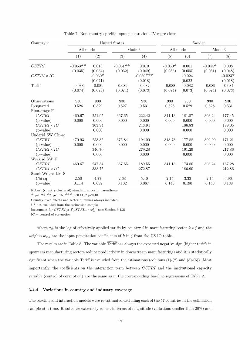
Table 7: Non country-specific input penetration: IV regressions

Country c United States Sweden

All modes Mode 3 All modes Mode 3

(1) (2) (3) (4) (5) (6) (7) (8)

CSTRI -0.053## 0.013 -0.051## 0.019 -0.050# 0.001 -0.044# 0.008(0.035) (0.054) (0.032) (0.049) (0.035) (0.055) (0.031) (0.048)

CSTRI × IC -0.030# -0.030### -0.024 -0.023#

(0.021) (0.018) (0.022) (0.018)Tariff -0.088 -0.081 -0.089 -0.082 -0.088 -0.082 -0.089 -0.084

(0.074) (0.073) (0.074) (0.073) (0.074) (0.073) (0.074) (0.073)

Observations 930 930 930 930 930 930 930 930R-squared 0.526 0.529 0.527 0.531 0.526 0.529 0.528 0.531First-stage FCSTRI 460.67 251.95 367.65 222.42 341.13 181.57 303.24 177.45(p-value) 0.000 0.000 0.000 0.000 0.000 0.000 0.000 0.000CSTRI × IC 303.94 243.94 186.83 189.05(p-value) 0.000 0.000 0.000 0.000

Underid SW Chi-sqCSTRI 470.93 253.35 375.84 194.00 348.73 177.88 309.99 171.21(p-value) 0.000 0.000 0.000 0.000 0.000 0.000 0.000 0.000CSTRI × IC 346.70 279.28 191.29 217.86(p-value) 0.000 0.000 0.000 0.000

Weak id SW FCSTRI 460.67 247.54 367.65 189.55 341.13 173.80 303.24 167.28CSTRI × IC 338.75 272.87 186.90 212.86

Stock-Wright LM SChi-sq 2.50 4.77 2.68 5.40 2.14 3.33 2.14 3.96(p-value) 0.114 0.092 0.102 0.067 0.143 0.190 0.143 0.138

Robust (country-clustered) standard errors in parentheses# p<0.20, ## p<0.15, ### p<0.11, * p<0.10

Country fixed effects and sector dummies always included

US not excluded from the estimation sample

Instrument for CSTRIij : ∑s STRIis ×wIVjs (see Section 3.4.2)

IC = control of corruption

where τik is the log of effectively applied tariffs by country i in manufacturing sector k ≠ j and the

weights wijk are the input penetration coefficients of k in j from the US IO table.

The results are in Table 8. The variable Tariff has always the expected negative sign (higher tariffs in

upstream manufacturing sectors reduce productivity in downstream manufacturing) and it is statistically

significant when the variable Tariff is excluded from the estimations (columns (1)-(2) and (5)-(6)). Most

importantly, the coefficients on the interaction term between CSTRI and the institutional capacity

variable (control of corruption) are the same as in the corresponding baseline regressions of Table 2.

3.4.4 Variations in country and industry coverage

The baseline and interaction models were re-estimated excluding each of the 57 countries in the estimation

sample at a time. Results are extremely robust in terms of magnitude (variations smaller than 20%) and

17

Figure 6: Impact of use unit increase in CSTRI (Mode 3) on y: Random assignement of w

−0.

010.

000.

01

Effe

ct o

n lo

g pr

oduc

tivity

1 2 3 4 5

Control of Corruption in year 2007

Estimated Impact 95% CI Mean Moderator

Table 8: Estimation with tariffs in other manufacturing sectors

All modes Mode 3

(1) (2) (3) (4) (5) (6) (7) (8)

CSTRI -0.024 0.063* -0.024 0.063 -0.038* 0.053 -0.038* 0.052(0.024) (0.038) (0.024) (0.038) (0.021) (0.032) (0.021) (0.032)

CSTRI × IC -0.041*** -0.041*** -0.039*** -0.039***(0.014) (0.014) (0.012) (0.012)

Tariff 0.002 0.013 -0.220 -0.204(0.139) (0.140) (0.371) (0.377)

Tariff -0.246* -0.232* -0.248 -0.252 -0.565* -0.534* -0.223 -0.217(0.136) (0.133) (0.216) (0.214) (0.297) (0.289) (0.599) (0.601)

Observations 912 912 912 912 912 912 912 912R-squared 0.523 0.526 0.523 0.526 0.524 0.528 0.524 0.528

Robust (country-clustered) standard errors in parentheses

* p<0.10, ** p<0.05, *** p<0.01

Country fixed effects and sector dummies always included

IC = control of corruption

statistical significance of the coefficients. Results remain quite robust when dropping each of the 18

manufacturing sectors at a time: the signs of the key coefficients are unchanged, although in a few cases

the coefficient of the interaction term varies more than 20% (never more than 50%). Results of these

300 regressions (57 plus 18 for Mode 3 and All modes, both with the baseline specification and the

specification with interaction) are available upon request.

18

4 Theory

In this section we propose a theoretical framework that provides some insights into the empirical finding

that institutional capacity is an important moderator variable for the positive effect of services trade

openness on productivity in downstream industries. The framework proposes two different channels

through which institutions can have an impact. The first channel centers on the trade decision (ex ante).

The second channel operates conditional on engaging in exports. A key feature of the framework is to

recognize that the proximity burden means that foreign suppliers must perform some part of the service

in the destination (importing) country. As a result, the institutional environment in the destination

country is a determinant of an exporter’s payoff. If institutions are not perfectly observable for firms that

are located abroad, the ability to identify countries with higher quality institutions will be one parameter

differentiating firms: only the best firms, those providing higher quality services, will have the capacity to

detect the best countries. Countries with high quality institutions will attract foreign firms that provide

on average better services than foreign firms in countries with weaker institutions. As a consequence, the

downstream industries in countries with high institutional capacity will benefit more from services trade

openness. This ‘selection effect’ is complemented by a second channel which is active given an export

decision (ex post). Both the exporters’ payoff and the quality of their services performance is sensitive

to the institutional environment in which they have decided to operate. Thus, for any level of exporters’

productivity, the average quality of foreign services performance in an institutionally weak environment

will be less than in countries with robust institutions.

4.1 The setup

The economy consists of two countries indexed by i ∈ {1,2}. The two countries have an identical economic

structure while they differ in terms of institutional setting, which we define as the capacity of a country to

minimise the exposure of the economic agents active within its territory to harmful unexpected changes

in the operating environment. This definition captures the different dimensions of institutional capacity

explored in our empirical exercise: from control of corruption, to rule of law, to regulatory quality.34

Each country is characterised by an industry Y using intermediate input x. We take a reduced form

approach assuming that the average productivity y in the downstream industry of country i is a function

of the average quality q of the intermediate input x available in the country. Formally,

yi = f(qi) ∀i (4.1)

with f strictly positive, increasing and concave and qi ∈ [0,1] ∀i. We assume that each country has a

minimum-quality domestic supply of x, such that, if the countries are closed to international transactions

34Examples include unexpected corruption episodes, restrictions on key complementary investments or movement ofpersonnel, sudden changes in the authorizing regulatory framework.

19

in x the productivity of the downstream sector is yi = f(0) ∀i.

The international supply of x consists of a continuum of heterogeneous exporters located outside the

two-country system described above and indexed by ϕ, which corresponds to a productivity parameter

varying on the support [0,1] such that exporter ϕ = 0 has a minimum productivity while exporter ϕ = 1

is the most productive. Exporters have to choose where to export x among the potential destination

countries. Once the destination country is chosen, trade takes place. However, because of the promity

burden, this often will involve a stage in which the foreign firm must undertake activities in the territory

of the selected destination country. To capture this, we introduce an intangibility parameter τ ∈ [0,1]

that determines the relative importance of this ‘performance stage’. This allows x to range from being

fully tangible (all production occurs in the exporting country) to fully intangible (all activities must be

performed in the importing nation). If it is fully tangible the product is called a ‘good’. In all other cases

it is a ‘service’. In the latter case, during the stage of services performance in the importing country i,

the foreign firm confronts unexpected shocks in the operating environment that follow a homogeneous

Poisson process with rate parameter θi. For each unexpected event the foreign firm incurs a unitary

cost which does not vary across destination countries. The expected payoff of exporting the intermediate

service input x with intangibility τ to country i is given by:

E[πi(ϕ)] = g(ϕ) − θiτ (4.2)

with g positive, increasing and concave. Toto restrict the analysis to exporters – i.e. to firms that get

non negative payoffs by exporting – we assume that g(0) > 1. θ captures the institutional setting in

country i with high values of θ being associated with fragile institutions. For simplicity we restrict35 the

support of θ to the interval (0,1]. Similarly, we assume that the quality of exporters’ output depends

positively on their productivity and negatively on the θ parameter of the selected destination country

in instances where x possesses some degree of intangibility: unexpected negative events not only affect

exporters’ payoffs but also the quality of their output x. Formally,

E[qi(ϕ)] = k(ϕ) − θiτ (4.3)

with k positive, increasing and concave. We assume that k(0) > 1 to focus on foreign firms that produce

higher quality than domestically supplied intermediate inputs. This assumption reflects the usual new

trade theory implication that exporting firms have superior properties than non-exporting ones. This

framework makes the exporter’s payoff as well as the quality of the exported output a function of the

institutional quality of the selected destination country in all cases where a product has some degree of

35This restriction makes the number of unexpected shocks a fraction instead of an integer without modifying the economicmeaning of the payoff function.

20

intangibility.36

Finally, we assume that the institutional capacity of potential destination countries is not perfectly

observable and that the productivity ϕ determines the precision with which an exporter can estimate the

true value of θ. For each potential destination country i, exporters observe a signal ϑi instead of θi. The

signals are independently distributed according to non-standard uniform probability density functions:

ϑi ∼ U[q1(θi, ϕ), q2(θi, ϕ)] ∀i (4.4)

where q1 = θiϕ and q2 = (θi − 1)ϕ + 1. This specification implies that an exporter with maximum

productivity (ϕ = 1) observes - for each potential destination country - a signal which is equal to the

true institutional capacity with probability 1. In contrast, the signal observed by an exporter with

0 productivity can take any value in the support of the institutional capacity parameter with equal

probability. In between those two extrema, the size of the interval upon which the signal is uniformly

distributed is a decreasing function of the exporter’s productivity type.37

4.2 Closed and open regimes: the role of institutions

We can now study - under two different institutional environments - the effect of upstream trade openness

on downstream productivity. We assume without loss of generality that country 1 has a higher institu-

tional capacity than country 2, i.e. θ1 < θ2. We denote with δ the difference θ2 − θ1. If the two countries

are closed to international transactions in x the productivity of the downstream sector is yi = f(0) ∀i.

We consider now the case where the two countries open their economies, creating a pool of potential des-

tinations for international exporters. Given ϕ and τ , each exporter has to decide its destination country

based on the realization of the signals ϑ1 and ϑ2. If x is fully tangible (τ = 0), institutional capacities do

not affect by construction the payoffs and the exporters choose each country with equal probability. If

instead τ > 0, an exporter with productivity ϕ chooses country 1 if and only if:38

g(ϕ) − ϑ1τ ≥ g(ϕ) − ϑ2τ ⇐⇒ ϑ1 ≤ ϑ2 (4.5)

Denote with Π(i∣ϕ, δ) or simply Π(i) the probability of choosing country i given productivity ϕ and

institutional difference δ. The properties of the probabilistic structure embedded in the exporters’ decision

36The type of activity associated with intangibility, mode 3 / FDI, also is used to produce tangible items (goods). Asimilar framework may well apply to FDI more generally but the mechanism modelled here is qualitatively different becausefirms producing goods have a choice between exporting and FDI. In the services context the proximity burden requiresFDI and / or mode 4 cross-border movement, whereas in the case of goods the export versus FDI decision will take intoaccount the institutional environment and result in more exports relative to FDI than what would be optimal absent theinstitutional factors. In the case of services it is not feasible to produce in the exporting country and thus the process ofperforming a service is more sensitive to the institutional environment in the importing country.

37A more parsimonious specification for an equivalent signalling technology is given by q1 and q2 satisfying the followingproperties: q1 ∶ (0,1]× [0,1]→ [0, θi] with q1(θi,0) = 0, q1(θi,1) = θi, ∂q1/∂θi ≥ 0, ∂q1/∂ϕ ≥ 0 and q2 ∶ (0,1]× [0,1]→ [θi, θ]with q2(θi,0) = 1, q2(θi,1) = θi, ∂q2/∂θi ≤ 0, ∂q2/∂ϕ ≤ 0.

38Having a weak inequality in the choice condition reflects our implicit assumption that, when the exporter receives twoidentical signals, it is ‘lucky’ and chooses the best country.

21

problem are given in the following Lemma.

Lemma 1 If x possesses some degree of intangibility (τ > 0),

(i) ∀δ > 0 and ϕ > 0, Π(1) > Π(2). If ϕ = 0, then Π(1) = Π(2);

(ii) the probability of choosing the best (worst) country is a non-decreasing (non-increasing) function of

both the exporters’ productivity ϕ and the difference in institutional capacity δ.

Proof. See Appendix C.

Lemma 1 point (i) states that, if the two countries are not identical, at any non-zero level of produc-

tivity the probability of choosing the best country is higher than the probability of choosing the worst

country. Moreover, Lemma 1, point (ii) formally restates the selection mechanism of our framework:

better exporters gets more precise signals about the institutional capacity of potential destination coun-

tries and therefore choose to export to the best country with a higher probability. Furthermore, given

our specification, the institutional difference between the two countries positively affects the precision of

the signal at any level of productivity. The probabilistic structure described in Lemma 1 determines the

expected average quality of the intermediate input available in each country, which corresponds to the

weighted average of the output’s expected quality across exporters, with weights given by the probability

of exporting to country i. Formally,

qi = ∫1

0E[qi(ϕ)] ×Π(i)dϕ (4.6)

An immediate corollary of Lemma 1 is given by the following

Corollary 1 If x possesses some degree of intangibility (τ > 0), then y1 > y2 > f(0).

Proof. See Appendix C.

Openness to trade in the non-fully-tangible intermediate input x increases downstream productivity

above its closed economy benchmark everywhere. This effect is higher in the country with a better

institutional framework. When comparing the weighted average of the expected quality qi of output in

the two countries, we can identify the two impact channels discussed at the beginning of this section.

The difference between the probability of choosing the best country and the probability of choosing

the worst, reflects the ex-ante impact channel of institutional capacity. This difference is a function of

exporters productivity. The difference between E[q1(ϕ)] and E[q2(ϕ)] is constant for any given level of

productivity and reflects the ex-post impact channel of institutions.

22

5 Conclusions

Services trade policy reform is an important ingredient for economic development, because services are

essential inputs into modern manufacturing. Due to the specificities of services and services trade,

however, reducing the restrictiveness of services trade policy may not be a sufficient condition for the

expected positive effect of liberalised service trade on downstream industries.

Using an empirical model that identifies the causal link between services liberalisation and down-

stream manufacturing productivity, this paper has shown that this conjecture is confirmed by the data.

Our estimates imply that the same reduction in services trade restrictiveness would increase manufactur-

ing productivity by 16.7% in a country with high institutional capacity such as Canada, as compared to

only 3.9% in a country with low institutional capacity such as Tanzania. Analogous differences hold for

countries at equivalent stages of economic development and with similar per capita incomes, like Austria

and Italy.

We have formalized these empirical results with a theoretical framework that incorporates the specific

characteristics of services and services trade – namely, exporting services firms must to a greater or lesser

extent engage in economic activity within importing countries. When international services transactions

are liberalised, cross-country differences in institutional capacity generates both a selection effect at the

level of the decision whether to engage in trade, and a performance effect that operates once trade

decisions have been taken. The interaction of the two factors allows manufacturing firms in countries

with good institutions to source higher quality services inputs. Our empirical exercise captures both of

these effects at the same time. An empirical quantification of the two effects requires firm-level data for

a broad cross-section of countries and is left for future research.

23

References

Acemoglu, D., S. Johnson, and J. Robinson, 2001, “The Colonial Origins of Comparative Development:

An Empirical Investigation,” American Economic Review, 91, 1369–1401.

Acemoglu, D., S. Johnson, and J. A. Robinson, 2005, “Institutions as a fundamental cause of long-run

growth,” in Philippe Aghion, and Steven N. Durlauf (ed.), Handbook of economic growth, Elsevier,

385-472.

Anderson, J. E., and D. Marcouiller, 2002, “Insecurity and the Pattern of Trade: an Empirical Investi-

gation,” Review of Economics and Statistics, 84, 342–352.

Antras, P., and E. Helpman, 2004, “Global Sourcing,” Journal of Political Economy, 112, 552–580.

Arnold, J. M., B. Javorcik, and A. Mattoo, 2011, “Does Services Liberalization Benefit Manufacturing

Firms? Evidence from the Czech Republic,” Journal of International Economics, 85, 136–146.

Arnold, J. M., B. Javorcik, and A. Mattoo, forthcoming, “Services Reform and Manufacturing Perfor-

mance. Evidence from India,” Economic Journal.

Arnold, J. M., A. Mattoo, and G. Narciso, 2008, “Services Inputs and Firm Productivity in Sub-Saharan

Africa: Evidence from Firm-Level Data,” Journal of African Economies, 17, 578–599.

Barone, G., and F. Cingano, 2011, “Service Regulation and Growth: Evidence from OECD Countries,”

Economic Journal, 121, 931–957.

Bernard, A., B. Jensen, S. Redding, and P. Schott, 2010, “Intrafirm Trade and Product Contractibility,”

American Economic Review Papers and Proceedings, 100, 444–448.

Blonigen, B. A., forthcoming, “Industrial Policy and Downstream Export Performance,” Economic Jour-

nal.

Blonigen, B. A., and J. Piger, 2014, “Determinants of foreign direct investment,” Canadian Journal of

Economics, 47, 775–812.

Borchert, I., B. Gootiiz, and A. Mattoo, 2012, “Guide to the Services Trade Restrictions Database,”

World Bank Policy Research Working Paper No. 6108.

Borghi, E., C. Del Bo, and M. Florio, forthcoming, “Institutions and Firms’ Productivity: Evidence from

Electricity Distribution in the EU,” Oxford Bulletin of Economics and Statistics.

Bourles, R., G. Cette, J. Lopez, J. Mairesse, and G. Nicoletti, 2013, “Do Product Market Regulations in

Upstream Sectors Curb Productivity Growth? Panel Data Evidence for OECD Countries,” Review of

Economics and Statistics, 95, 1750–1768.

24

Chor, D., 2010, “Unpacking sources of comparative advantage: A quantitative approach,” Journal of

International Economics, 82, 152–167.

Ciccone, A., and E. Papaioannou, 2006, “Adjustment to Target Capital, Finance and Growth,” CEPR

Discussion Paper No. 5969.

Costinot, A., 2009, “On the origins of comparative advantage,” Journal of International Economics, 77,

255–264.

Dollar, D., M. Hallward-Driemeier, and T. Mengistae, 2005, “Investment Climate and Firm Performance

in Developing Economies,” Economic Development and Cultural Change, 54, 1–31.

Duggan, V., S. Rahardja, and G. Varela, 2013, “Service Sector Reform and Manufacturing Productivity.

Evidence from Indonesia,” World Bank Policy Research Working Paper No. 6349.

Fernandes, A., and C. Paunov, 2011, “Foreign Direct Investment in Services and Manufacturing Produc-

tivity: Evidence for Chile,” Journal of Development Economics, 97, 305–321.

Forlani, E., 2012, “Competition in the service sector and the performances of manufacturing firms: does

liberalization matter?,” CESifo Working Paper No. 2942.

Gaviria, A., 2002, “Assessing the effects of corruption and crime on firm performance: evidence from

Latin America,” Emerging Markets Review, 3, 245–268.

Goldberg, P. K., A. K. Khandelwal, N. Pavcnik, and P. Topalova, 2010, “Imported Intermediate Inputs

and Domestic Product Growth: Evidence from India,” Quarterly Journal of Economics, 125, 1727–

1767.

Grossman, G., and E. Helpman, 2005, “Outsourcing in a Global Economy,” Review of Economic Studies,

72, 135.

Helpman, E., 1987, “Imperfect competition and international trade: Evidence from fourteen industrial

countries,” Journal of the Japanese and International Economies, 1, 62–81.

Hoekman, B., and B. Shepherd, forthcoming, “Services Productivity, Trade Policy, and Manufacturing

Exports,” The World Economy.

Johnson, R. C., 2014, “Five Facts about Value-Added Exports and Implications for Macroeconomics and

Trade Research,” Journal of Economic Perspectives, 28, 119–42.

Jones, C. I., 2011, “Intermediate Goods and Weak Links in the Theory of Economic Development,”

American Economic Journal: Macroeconomics, 3, 1–28.

25

Keller, W., 1998, “Are international R&D spillovers trade-related? Analyzing spillovers among randomly

matched trade partners,” European Economic Review, 42, 469–481.

Lensink, R., and A. Meesters, 2014, “Institutions and Bank Performance: A Stochastic Frontier Analysis,”

Oxford Bulletin of Economics and Statistics, 76, 67–92.

Levchenko, A., 2007, “Institutional Quality and International Trade,” Review of Economic Studies, 74,

791–819.

Nunn, N., 2007, “Relationship-Specificity, Incomplete Contracts, and the Patterns of Trade,” Quarterly

Journal of Economics, 122, 569–600.

O’Mahony, M., and M. P. Timmer, 2009, “Output, Input and Productivity Measures at the Industry

Level: The EU KLEMS Database,” Economic Journal, 119, F374–F403.

Papke, L., and J. Wooldridge, 1996, “Econometric methods for fractional response variables with an

application to 401(k) plan participation rates,” Journal of Applied Econometrics, 11, 619–632.

Parry, G., L. Newnes, and X. Huang, 2011, “Goods, Products and Services,” in Mairi Macintyre, Glenn

Parry, and Jannis Angelis (ed.), Services Design and Delivery: Research and Innovations in the Service

Economy, Springer Science and Business Media, 19-29.

Rajan, R. G., and L. Zingales, 1998, “Financial Dependence and Growth,” American Economic Review,

88, 559–586.

Rodriguez, F., and D. Rodrik, 2014, “Trade policy and economic growth: a skeptic’s guide to the cross-

national evidence,” in Ben S. Bernanke, and Kenneth Rogoff (ed.), NBER Macroeconomics Annual,

MIT Press.

Rodrik, D., 2013, “Unconditional Convergence in Manufacturing,” Quarterly Journal of Economics, 128,

165–204.

Rodrik, D., A. Subramanian, and F. Trebbi, 2004, “Institutions Rule: The Primacy of Institutions Over

Geography and Integration in Economic Development,” Journal of Economic Growth, 9, 131–165.

Sanderson, E., and F. Windmeijer, forthcoming, “A Weak Instrument F-Test in Linear IV Models with

Multiple Endogenous Variables,” Journal of Econometrics.

Topalova, P., and A. Khandelwal, 2011, “Trade Liberalization and Firm Productivity: The Case of India,”

Review of Economics and Statistics, 93, 995–1009.

Van Ark, B., M. O’Mahony, and M. P. Timmer, 2008, “The productivity gap between Europe and the

united States: trends and causes,” Journal of Economic Perspectives, 22, 25–44.

26

van der Marel, E., 2014a, “Does Comparative Advantage Induce Autonomous Liberalization? The

Case of Services,” unpublished manuscript. Available at www.freit.org/WorkingPapers/Papers/

TradePolicyGeneral/FREIT720.pdf.

van der Marel, E., 2014b, “New sources of comparative advantage in services trade,” presented at the

conference “New Horizons in Services Trade Governance” (Geneva, 25-26 November 2014).

van der Marel, E., and S. Miroudot, 2014, “The Economics and Political Economy of Going Beyond the

GATS,” Review of International Organizations, 9, 205–239.

Winters, L. A., and A. Masters, 2013, “Openness and Growth: Still an Open Question?,” Journal of

International Development, 25, 1061–1070.

World Trade Organization (WTO), 2013, World Trade Report 2013. Factors shaping the future of world

trade, World Trade Organization, Geneva.

27

Appendices

A Appendix tables

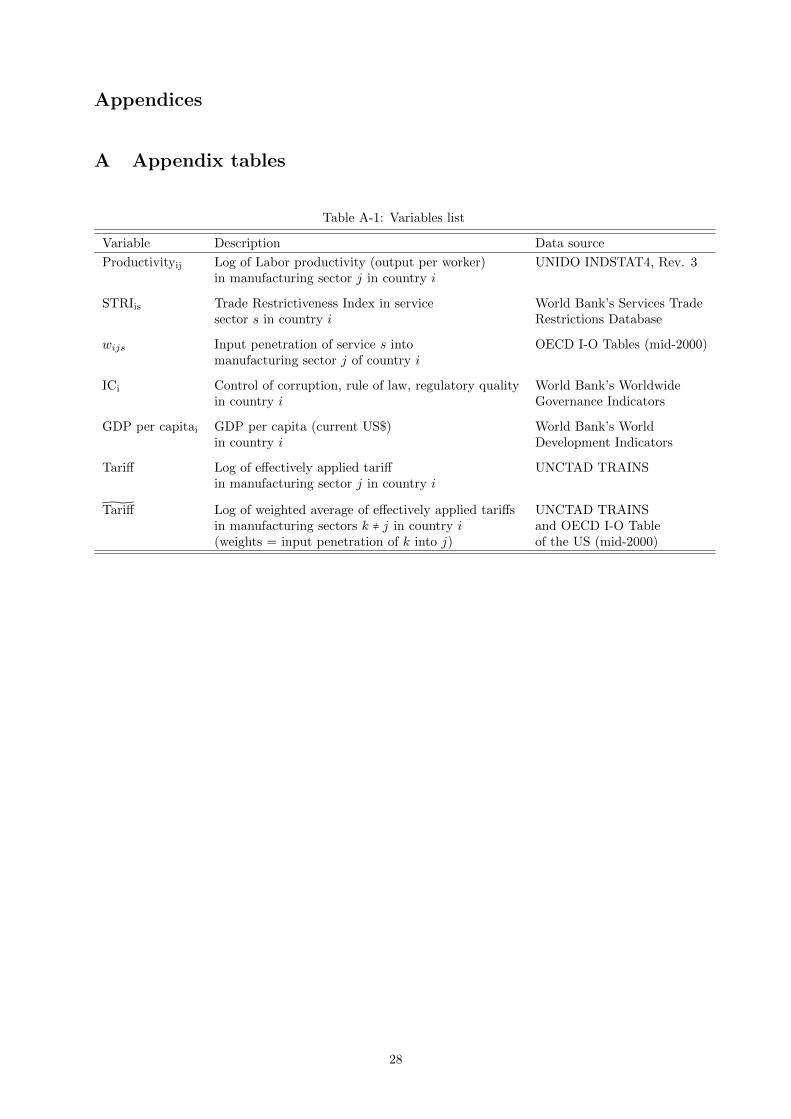
Table A-1: Variables list

Variable Description Data source

Productivityij Log of Labor productivity (output per worker) UNIDO INDSTAT4, Rev. 3in manufacturing sector j in country i

STRIis Trade Restrictiveness Index in service World Bank’s Services Tradesector s in country i Restrictions Database

wijs Input penetration of service s into OECD I-O Tables (mid-2000)manufacturing sector j of country i

ICi Control of corruption, rule of law, regulatory quality World Bank’s Worldwidein country i Governance Indicators

GDP per capitai GDP per capita (current US$) World Bank’s Worldin country i Development Indicators

Tariff Log of effectively applied tariff UNCTAD TRAINSin manufacturing sector j in country i

Tariff Log of weighted average of effectively applied tariffs UNCTAD TRAINSin manufacturing sectors k ≠ j in country i and OECD I-O Table(weights = input penetration of k into j) of the US (mid-2000)

28

Table A-2: List of countries and sectors in the estimations

Country Sector

Albania Kyrgyz Rep. 15-16Austria Lebanese Rep. 17-19Belgium Lithuania 20Botswana Malawi 21-22Brazil Malaysia 23Bulgaria Mauritius 24Burundi Mongolia 25Canada Morocco 26Chile Netherlands 27China New Zealand 28Colombia Oman 29Czech Republic Peru 30Denmark Poland 31Ecuador Portugal 32Ethiopia Qatar 33Finland Romania 34France Saudi Arabia 35Georgia South Africa 36-37Germany SpainGreece Sri LankaHungary SwedenIndia TanzaniaIndonesia TurkeyIreland UkraineItaly United KingdomJapan UruguayJordan Viet NamKorea, Rep. YemenKuwait

Sectors are ISIC Rev. 3 manufacturing industries

29

B Input Penetration Measures

Shares of intermediate consumption

Shares of intermediate consumption are derived from the first quadrant of the Input-Output (IO) matrix,

i.e. the intermediate demand matrix M . M is a square matrix of dimension n where rows – indexed by

r – are the supplying industries (domestic and international) and the columns – c – the using (domestic)

industries. The number of industries in the IO table is equal to n. A generic element mrc of the matrix

M is the cost borne by sector c for the output produced by sector j (domestic production plus imported

foreign production) and used as intermediate input into c. For each services-manufacturing sector pair

(s, j), s’ share of j’s total intermediate consumption is equal to:

wjs ≡msj

∑nr=1mrj

(B-1)

IO technical coefficients

IO technical coefficients are the elements of the square matrix A, defined as:

A ≡ YM (B-2)

where Y is a dimension n square matrix of zeros, except along the main diagonal, that includes the inverse

output of each industry. For each services-manufacturing sector pair (s, j), the IO technical coefficient

is the element asj of matrix A and it gives the cost of the intermediate inputs from services sector s for

one dollar of total production of manufacturing sector j.

Leontief coefficients

The third input penetration measure used in the paper consists of the coefficients derived from the

Leontief inverse matrix. The input penetration of services sector s into manufacturing sector j that takes

into account the indirect linkages between the supplying and the using sectors is given by the element lsj

of matrix L, defined as:

L ≡ V B (B-3)

where V is a dimension n square matrix of zeros, except along the main diagonal, that includes the value

added-output ratios of each industry. B is the Leontief inverse (I − A)−1, with A defined in equation

(B-2) above.

30

C Proofs

Proof of Lemma 1. We assume WLOG that θ1 < θ2. The probability of choosing the best country

Π(1) is given by:

Π(1) = Pr(ϑ1 ≤ ϑ2) = Pr(ϑ1 − ϑ2 ≤ 0) = FZ(0) (C-1)

where Z is the random variable function of the two signals, Z ≡ ϑ1 − ϑ2, and FZ is its cumulative

distribution function. In order to derive the analytical expression for FZ(0) we need to integrate the

joint distribution of the two independent random variables ϑ1 and ϑ2 over the area in the joint support

on the (ϑ1, ϑ2)-plane where ϑ2 ≥ ϑ1. The joint pdf p(⋅, ⋅) of two independent random variables is the

product of their distributions, therefore:

p(ϑ1, ϑ2) =1

q2(θ1, ϕ) − q1(θ1, ϕ)×

1

q2(θ2, ϕ) − q1(θ2, ϕ)(C-2)

and, given our specification of the functions q1(θi, ϕ) and q2(θi, ϕ):

p(ϑ1, ϑ2) =1

(1 − ϕ)2(C-3)

Notice that the condition θ1 < θ2 plus our specification of q1(θi, ϕ) and q2(θi, ϕ) imply the following two

inequalities:

q1(θ1, ϕ) = θ1ϕ < θ2ϕ = q1(θ2, ϕ) ∀ϕ > 0 (C-4)

q2(θ1, ϕ) = (θ1 − 1)ϕ + 1 < (θ2 − 1)ϕ + 1 = q2(θ2, ϕ) ∀ϕ > 0 (C-5)

that become identities for ϕ = 0. (C-4) and (C-5) imply that the two points (q1(θ1, ϕ), q1(θ2, ϕ)) and

(q2(θ1, ϕ), q2(θ2, ϕ)) lie always above the 45 degree line in the (ϑ1, ϑ2)-plane. In order to identify the

area in the joint support of ϑ2 and ϑ1 where ϑ2 ≥ ϑ1 we just have to distinguish the following two cases:

1. if q2(θ1, ϕ) > q1(θ2, ϕ) which, given our specifications is equivalent to the condition ϕ < 1/(1 + δ),

the area where the joint pdf has to be integrated is given in Figure C-1;

2. if instead q2(θ1, ϕ) ≤ q1(θ2, ϕ), which means ϕ ≥ 1/(1 + δ), we have that the area where the joint

pdf has to be integrated is given in Figure C-2.

We have now all the ingredients to write the following expression for FZ(0):

FZ(0) =

⎧⎪⎪⎨⎪⎪⎩

∫q1(θ2,ϕ)q1(θ1,ϕ) ∫

q2(θ2,ϕ)q1(θ2,ϕ) p(ϑ1, ϑ2)dϑ2dϑ1 + ∫

q2(θ1,ϕ)q1(θ2,ϕ) ∫

q2(θ2,ϕ)ϑ1

p(ϑ1, ϑ2)dϑ2dϑ1 if 0 ≤ ϕ < 11+δ

∫q2(θ2,ϕ)q1(θ1,ϕ) ∫

q2(θ2,ϕ)q1(θ2,ϕ) p(ϑ1, ϑ2)dϑ2dϑ1 if 1

1+δ ≤ ϕ ≤ 1

(C-6)

Plugging the expressions for the joint distribution p(ϑ1, ϑ2), for q1(θ2, ϕ), for q2(θ2, ϕ) and rearranging

we get:

Π(1) = FZ(0) =

⎧⎪⎪⎨⎪⎪⎩

12+

δϕ1−ϕ[1 −

12δϕ

1−ϕ] if 0 ≤ ϕ < 11+δ

1 if 11+δ ≤ ϕ ≤ 1

(C-7)

The probability of choosing country 2 is then:

Π(2) = 1 − FZ(0) =

⎧⎪⎪⎨⎪⎪⎩

12[ϕ(1+δ)−1(1−ϕ)2 ]

2if 0 ≤ ϕ < 1

1+δ0 if 1

1+δ ≤ ϕ ≤ 1(C-8)

Point (i) and (ii) easily follow from the study of Π(1) and Π(2).

Proof of Corollary 1. if τ > 0, by construction we have that E[q1(ϕ)] > E[q2(ϕ)] > 0 ∀ϕ > 0 and

31

E[q1(ϕ)] = E[q2(ϕ)] > 0 for ϕ = 0. Moreover, from point (ii) of Lemma 1 we know that Π(1) > Π(2) ∀ϕ > 0

and Π(1) = Π(2) for ϕ = 0. Finally, again from Lemma 1 we know that there are many values of ϕ and δ

for which both Π(1) and Π(2) are strictly positive. It follows that:

q1 = ∫

1

0E[q1(ϕ)] ×Π(1)dϕ > ∫

1

0E[q2(ϕ)] ×Π(2)dϕ = q2 > 0 (C-9)

The result follows by construction given that yi = f(qi) with f strictly positive and increasing.

Figure C-1: area in the joint support where ϑ2 ≥ ϑ1 (case 1)

ϑ10

ϑ2

q1(θ1, ϕ) q2(θ1, ϕ)

ϑ1 = q1(θ2, ϕ)

q1(θ2, ϕ)

q2(θ2, ϕ)

ϑ2 = ϑ1

32

Figure C-2: area in the joint support where ϑ2 ≥ ϑ1 (case 2)

ϑ10

ϑ2

q1(θ1, ϕ) q2(θ1, ϕ)

q1(θ2, ϕ)

q2(θ2, ϕ)

ϑ2 = ϑ1

33