session 2. applied regression -- prof. juran2 outline for session 2 more simple regression –bottom...
TRANSCRIPT

Session 2

Applied Regression -- Prof. Juran 2
Outline for Session 2• More Simple Regression
– Bottom Part of the Output • Hypothesis Testing
– Significance of the slope and intercept parameters
• Interval Estimation– Confidence intervals for the slope and
intercept parameters
Applied Regression -- Prof. Juran 3
Computer Repair Example
123456789
101112131415161718
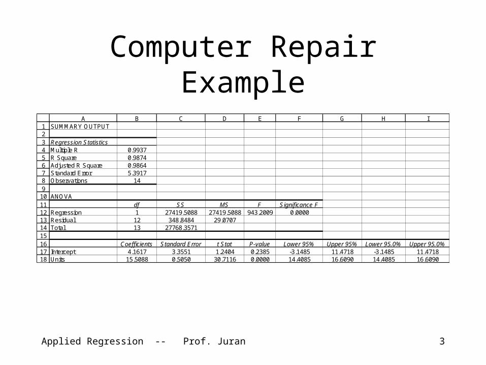
A B C D E F G H ISUMMARY OUTPUT
Regression StatisticsMultiple R 0.9937R Square 0.9874Adjusted R Square 0.9864Standard Error 5.3917Observations 14
ANOVAdf SS MS F Significance F
Regression 1 27419.5088 27419.5088 943.2009 0.0000Residual 12 348.8484 29.0707Total 13 27768.3571
Coefficients Standard Error t Stat P-value Lower 95% Upper 95% Lower 95.0% Upper 95.0%Intercept 4.1617 3.3551 1.2404 0.2385 -3.1485 11.4718 -3.1485 11.4718Units 15.5088 0.5050 30.7116 0.0000 14.4085 16.6090 14.4085 16.6090
Applied Regression -- Prof. Juran 4
Interpreting the Coefficients
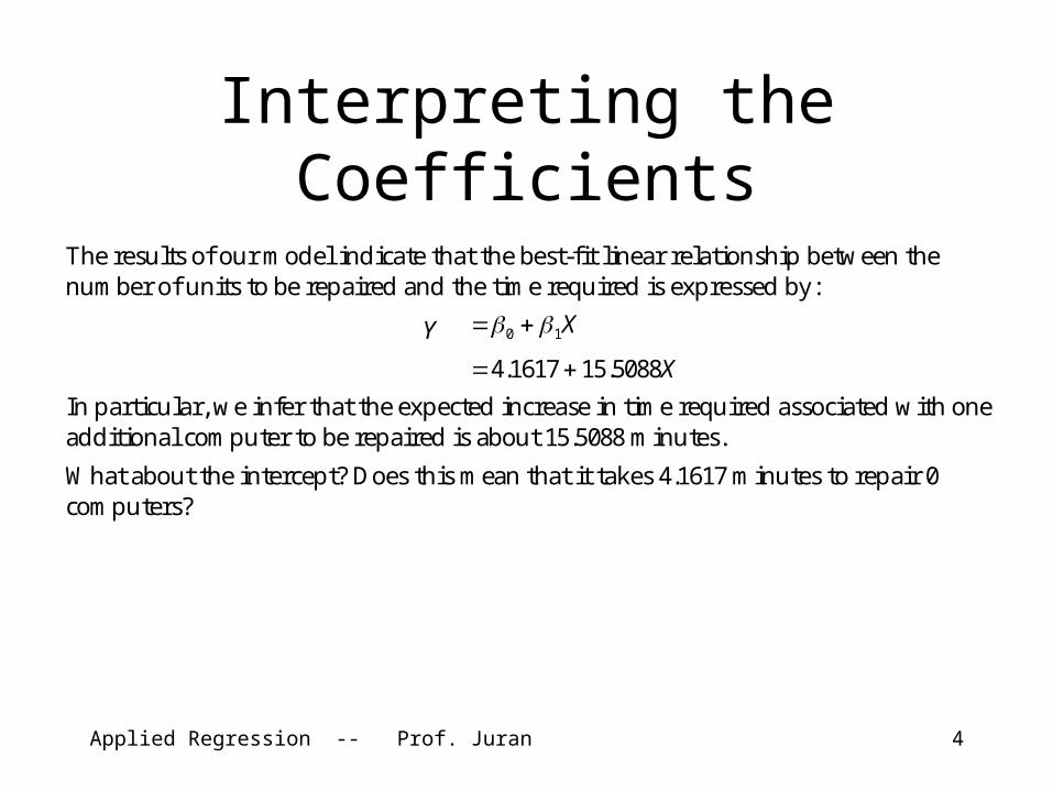
The results of our model indicate that the best-fit linear relationship between the number of units to be repaired and the time required is expressed by:
Y X10
X5088.151617.4
In particular, we infer that the expected increase in time required associated with one additional computer to be repaired is about 15.5088 minutes.
What about the intercept? Does this mean that it takes 4.1617 minutes to repair 0 computers?
Applied Regression -- Prof. Juran 5
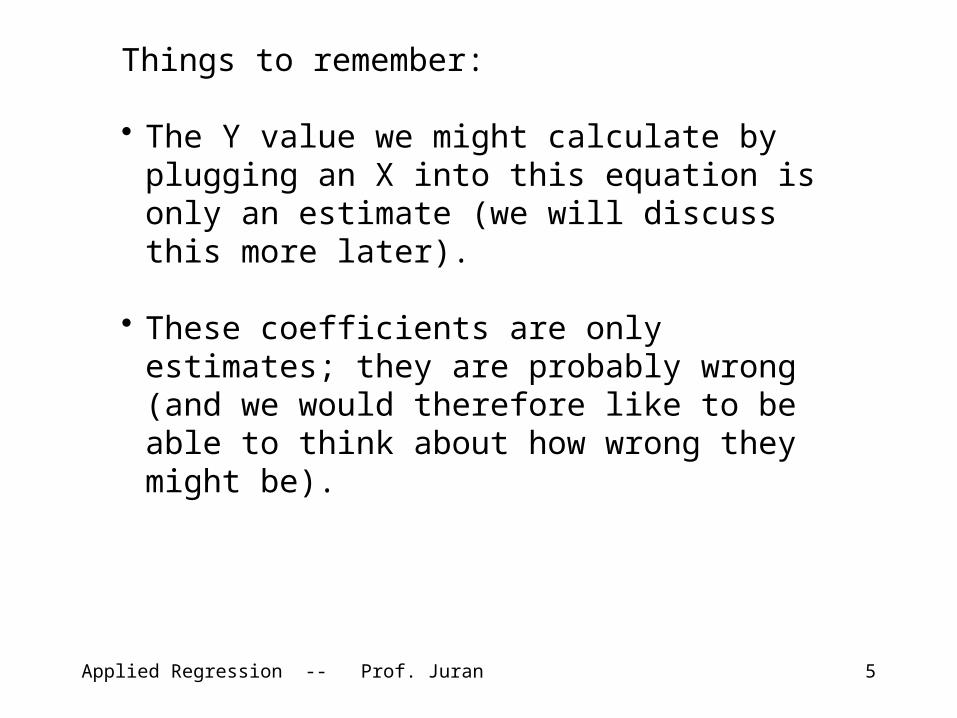
Things to remember:
• The Y value we might calculate by plugging an X into this equation is only an estimate (we will discuss this more later).
• These coefficients are only estimates; they are probably wrong (and we would therefore like to be able to think about how wrong they might be).

Applied Regression -- Prof. Juran 6
Significance of the Coefficients
• Are the slope and intercept significantly different from zero?
• Can we construct a confidence interval around these coefficients?
• We need measures of dispersion for the estimated parameters.

Applied Regression -- Prof. Juran 7
Statistics of the Regression Estimates
• If the true model is linear, the regression estimates are unbiased (correct expected value).
• If the true model is linear, the errors are uncorrelated, and the residual variance is constant in X, the regression estimates are also efficient (low variance relative to other estimators).
Applied Regression -- Prof. Juran 8
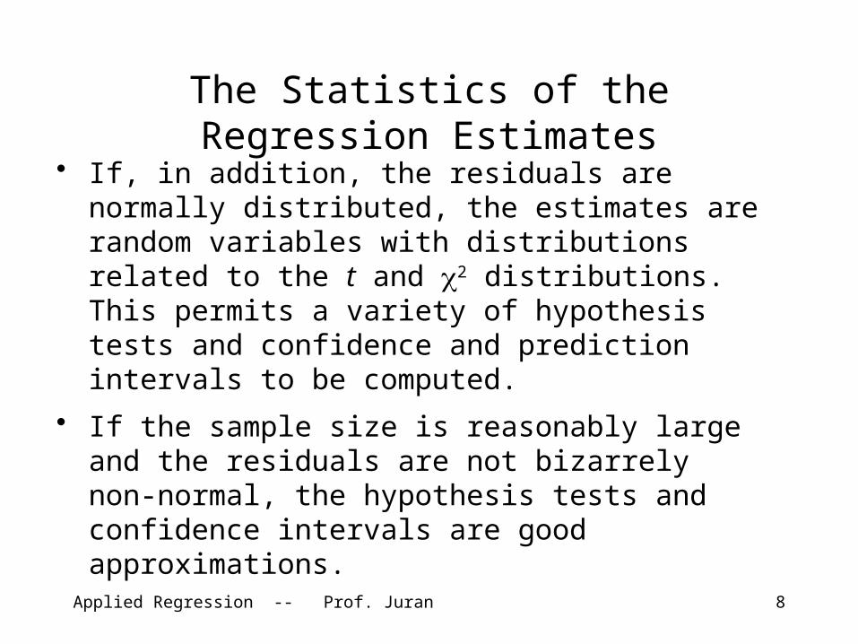
The Statistics of the Regression Estimates
• If, in addition, the residuals are normally distributed, the estimates are random variables with distributions related to the t and 2 distributions. This permits a variety of hypothesis tests and confidence and prediction intervals to be computed.
• If the sample size is reasonably large and the residuals are not bizarrely non-normal, the hypothesis tests and confidence intervals are good approximations.
Applied Regression -- Prof. Juran 9
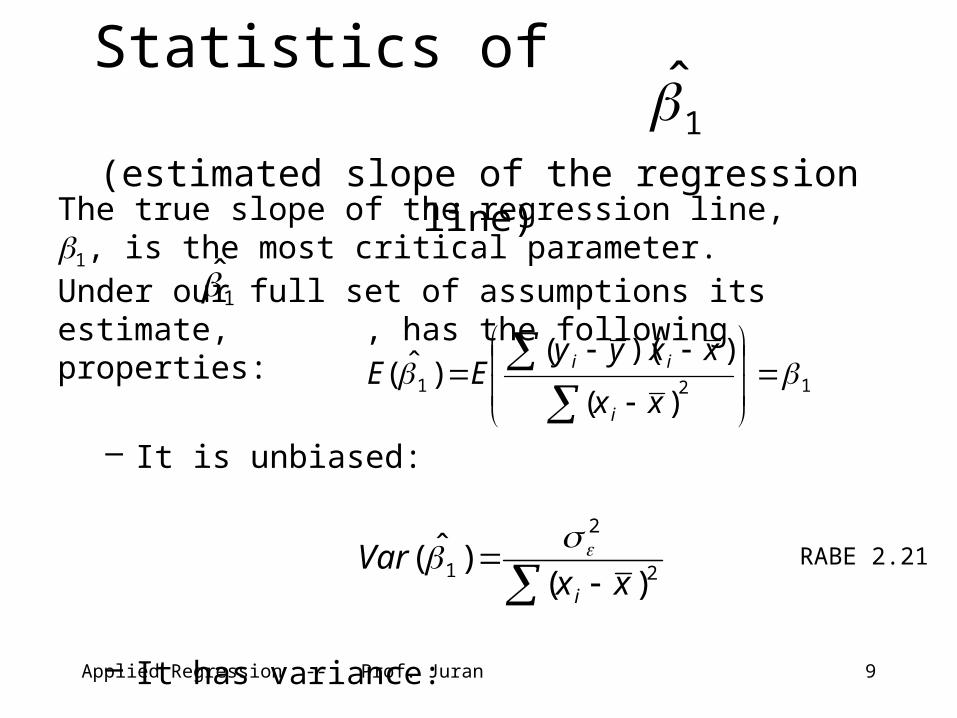
Statistics of (estimated slope of the regression line)
The true slope of the regression line, 1, is the most critical parameter. Under our full set of assumptions its estimate, , has the following properties:
– It is unbiased:
– It has variance:
121)(
))(()ˆ(
xx
xxyyEE
i
ii
1̂
1̂
2
2
1 )()ˆ(
xxVar
i
RABE 2.21
Applied Regression -- Prof. Juran 10
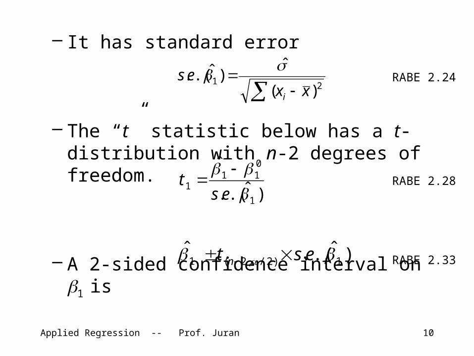
– It has standard error
– The “t” statistic below has a t-distribution with n-2 degrees of freedom.
– A 2-sided confidence interval on 1 is
)ˆ.(.
ˆ
1
011
1
est
)ˆ.(.ˆ1)2/,2(1 est n
RABE 2.24
RABE 2.28
RABE 2.33
21)(
ˆ)ˆ.(.
xxes
i
Applied Regression -- Prof. Juran 11
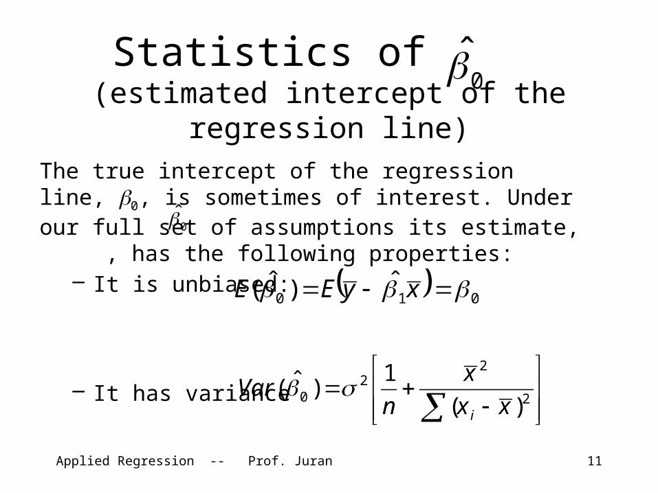
Statistics of (estimated intercept of the
regression line)The true intercept of the regression line, 0, is sometimes of interest. Under our full set of assumptions its estimate, , has the following properties:
– It is unbiased:
– It has variance
0̂
0̂
010ˆ)ˆ( xyEE
2
22
0 )(1
)ˆ(xx
xn
Vari
Applied Regression -- Prof. Juran 12
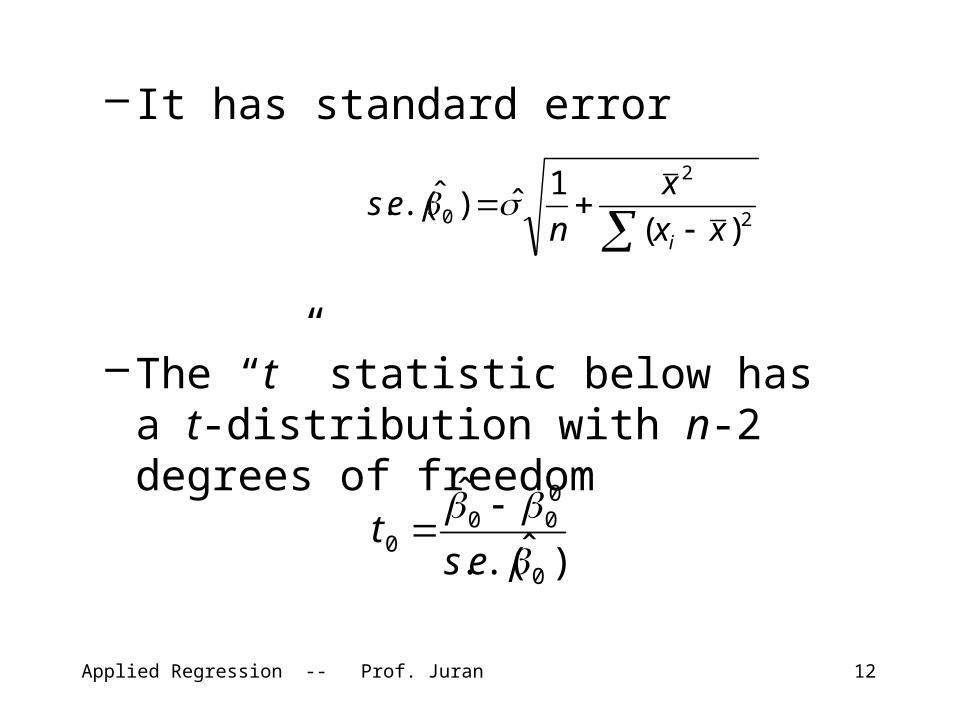
– It has standard error
–The “t” statistic below has a t-distribution with n-2 degrees of freedom
)ˆ.(.
ˆ
0
000
0
est
2
2
0 )(
1ˆ)ˆ.(.
xx
x
nes
i

Applied Regression -- Prof. Juran 13
4-Step Hypothesis Testing Procedure
1. Formulate Two Hypotheses
2. Select a Test Statistic
3. Derive a Decision Rule
4. Calculate the Value of the Test Statistic; Invoke the Decision Rule in light of the Test Statistic
Applied Regression -- Prof. Juran 14
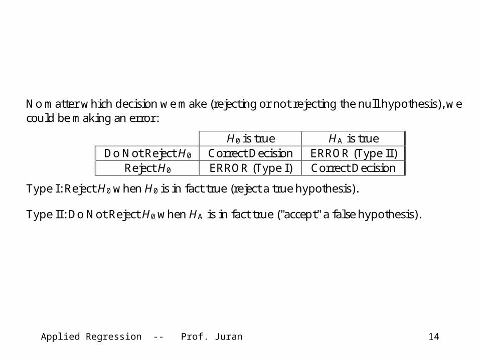
No matter which decision we make (rejecting or not rejecting the null hypothesis), we could be making an error:
H0 is true HA is true Do Not Reject H0 Correct Decision ERROR (Type II)
Reject H0 ERROR (Type I) Correct Decision
Type I: Reject H0 when H0 is in fact true (reject a true hypothesis).
Type II: Do Not Reject H0 when HA is in fact true ("accept" a false hypothesis).

Applied Regression -- Prof. Juran 15
Let = probability of a Type I Error = P(reject H0 | H0 is true),
= probability of a Type II Error = P("accept" H0 | HA is true).
The best we can do is to try to minimize these probabilities of error. As we will see, alpha is entirely under our control. Beta is not directly controllable in practical situations, but can be reduced with larger sample size.

Applied Regression -- Prof. Juran 16
Testing the significance of a simple linear regression ( 1 =
0? )
If the slope is zero (or, equivalently, if the correlation is zero) we do not have a relationship. Thus, a fundamental test is:
H0: 1 = 0
versus
HA: 1 0
Applied Regression -- Prof. Juran 17
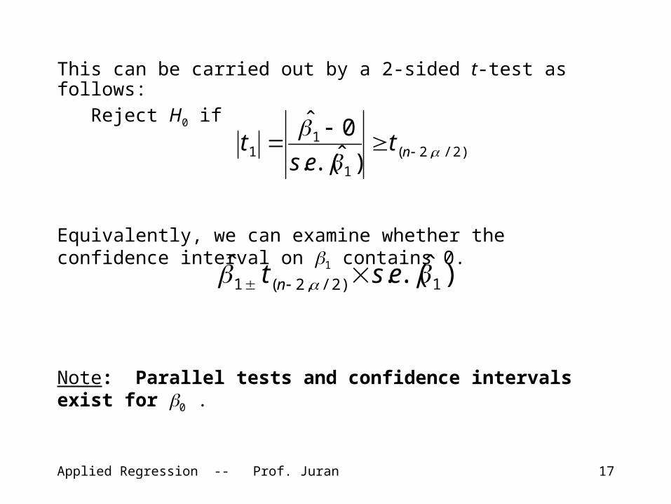
This can be carried out by a 2-sided t-test as follows:Reject H0 if
Equivalently, we can examine whether the confidence interval on 1 contains 0.
Note: Parallel tests and confidence intervals exist for 0 .
)2/,2(1
11
)ˆ.(.
0ˆ
nt
est
)ˆ.(.ˆ1)2/,2(1 est n
Applied Regression -- Prof. Juran 18
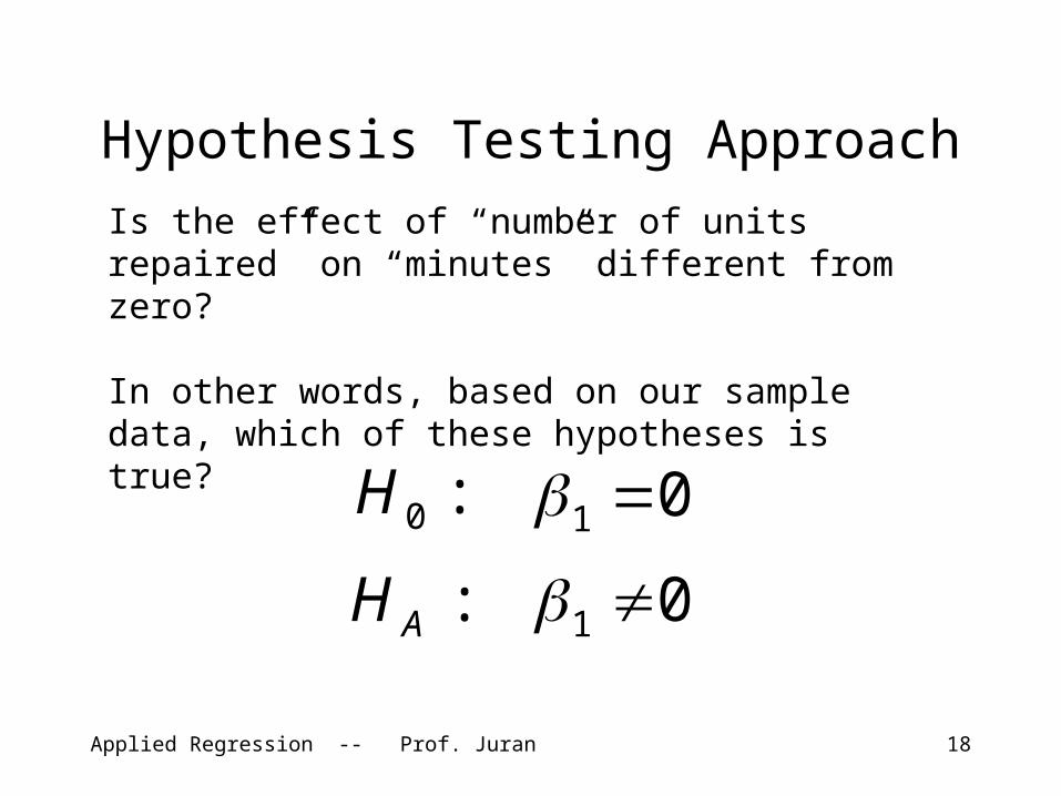
Is the effect of “number of units repaired” on “minutes” different from zero?
In other words, based on our sample data, which of these hypotheses is true?
:0H 01
:AH 01
Hypothesis Testing Approach
Applied Regression -- Prof. Juran 19
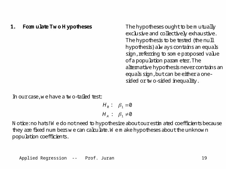
1. Formulate Two Hypotheses The hypotheses ought to be mutually exclusive and collectively exhaustive. The hypothesis to be tested (the null hypothesis) always contains an equals sign, referring to some proposed value of a population parameter. The alternative hypothesis never contains an equals sign, but can be either a one-sided or two-sided inequality.
In our case, we have a two-tailed test:
:0H 01
:AH 01
Notice: no hats! We do not need to hypothesize about our estimated coefficients because they are fixed numbers we can calculate. We make hypotheses about the unknown population coefficients.

Applied Regression -- Prof. Juran 20
2. Select a Test Statistic The test statistic is a standardized estimate of the difference between our sample and some hypothesized population parameter. It answers the question: “If the null hypothesis were true, how many standard deviations is our sample away from where we expected it to be?”
In our case, and assuming the null hypothesis is true, the sample slope coefficient will be t-distributed with a mean of zero and an estimated standard error from our regression output. We will use the t-statistic, measuring the number of standard errors our estimated slope is away from the hypothesized zero:
)ˆ.(.
0ˆ
1
11
es
t
Applied Regression -- Prof. Juran 21
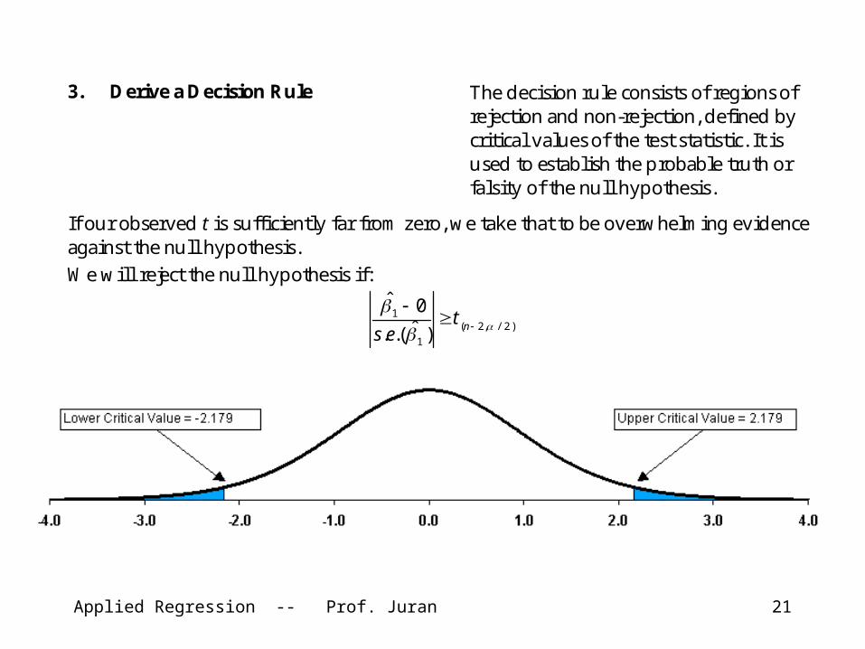
3. Derive a Decision Rule The decision rule consists of regions of rejection and non-rejection, defined by critical values of the test statistic. It is used to establish the probable truth or falsity of the null hypothesis.
If our observed t is sufficiently far from zero, we take that to be overwhelming evidence against the null hypothesis. We will reject the null hypothesis if:
)2/,2(1
1
)ˆ.(.
0ˆ
nt
es
Applied Regression -- Prof. Juran 22
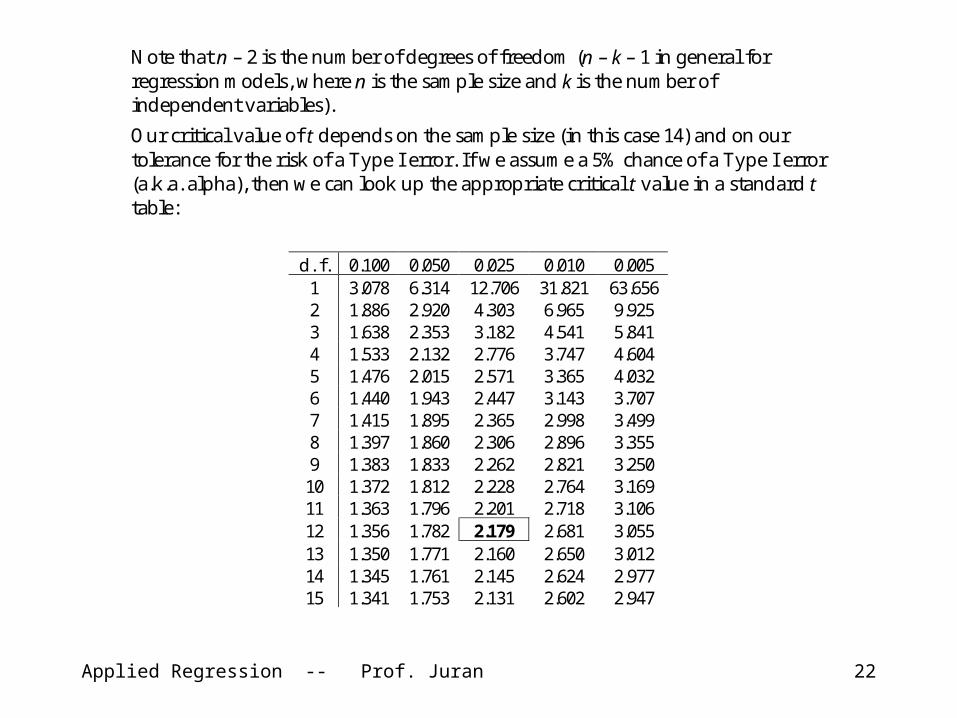
Note that n – 2 is the number of degrees of freedom (n – k – 1 in general for regression models, where n is the sample size and k is the number of independent variables).
Our critical value of t depends on the sample size (in this case 14) and on our tolerance for the risk of a Type I error. If we assume a 5% chance of a Type I error (a.k.a. alpha), then we can look up the appropriate critical t value in a standard t table:
d. f. 0.100 0.050 0.025 0.010 0.005 1 3.078 6.314 12.706 31.821 63.656 2 1.886 2.920 4.303 6.965 9.925 3 1.638 2.353 3.182 4.541 5.841 4 1.533 2.132 2.776 3.747 4.604 5 1.476 2.015 2.571 3.365 4.032 6 1.440 1.943 2.447 3.143 3.707 7 1.415 1.895 2.365 2.998 3.499 8 1.397 1.860 2.306 2.896 3.355 9 1.383 1.833 2.262 2.821 3.250 10 1.372 1.812 2.228 2.764 3.169 11 1.363 1.796 2.201 2.718 3.106 12 1.356 1.782 2.179 2.681 3.055 13 1.350 1.771 2.160 2.650 3.012 14 1.345 1.761 2.145 2.624 2.977 15 1.341 1.753 2.131 2.602 2.947
Applied Regression -- Prof. Juran 23
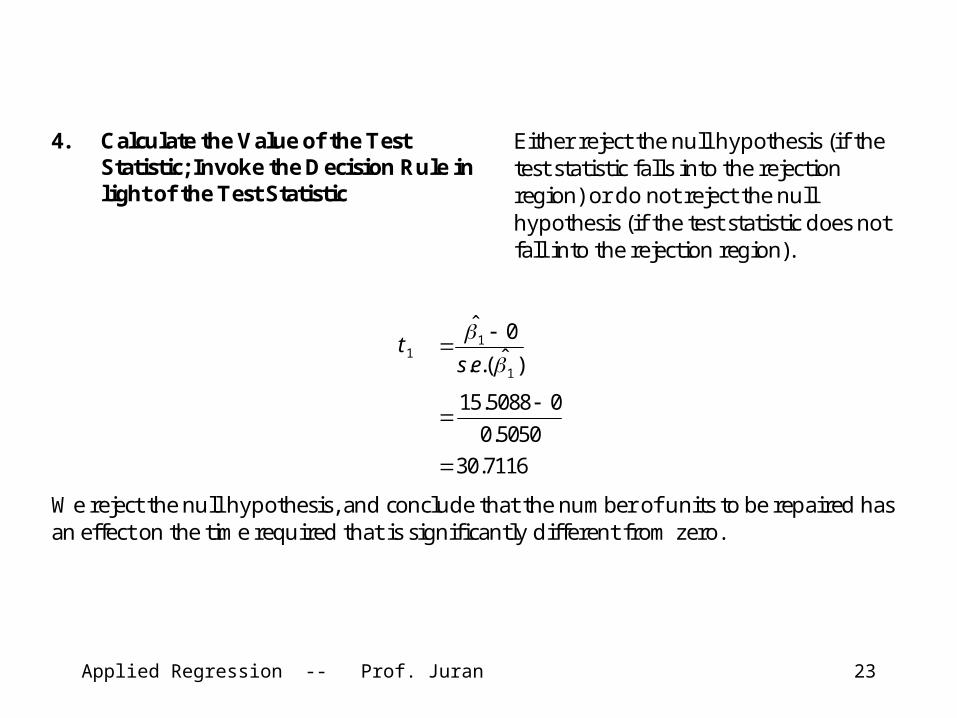
4. Calculate the Value of the Test Statistic; Invoke the Decision Rule in light of the Test Statistic
Either reject the null hypothesis (if the test statistic falls into the rejection region) or do not reject the null hypothesis (if the test statistic does not fall into the rejection region).
1t )ˆ.(.
0ˆ
1
1
es
5050.0
05088.15
7116.30
We reject the null hypothesis, and conclude that the number of units to be repaired has an effect on the time required that is significantly different from zero.
Applied Regression -- Prof. Juran 24
The p-value
The classical hypothesis testing method gives only a “reject” or “do not reject” answer; it doesn’t reveal all of the quantitative information inherent in the calculations we just performed. We might also want to know “How likely is it, under the assumption that the null hypothesis is true, that we would have a sample coefficient as far away as this from the null-hypothesized value?” In other words, “We observe an estimated slope of 15.5088. How likely would that be if the true population slope were really zero?” This probability is given by the p-value, which in this example is astronomically small. Our observed value is more than 30 standard errors away from its expected value under the null hypothesis.

Applied Regression -- Prof. Juran 25
What about the intercept?
It would appear that our estimated intercept here is not significantly different from zero (see the p-value of 0.2385).
It is not uncommon in practical situations to ignore a lack of significance in the intercept — the intercept is held to a lower standard of significance than the slope (or slopes).
Applied Regression -- Prof. Juran 26
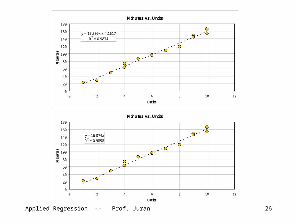
Minutes vs. Units
y = 15.509x + 4.1617
R2 = 0.9874
0
20
40
60
80
100
120
140
160
180
0 2 4 6 8 10 12
Units
Min
ute
s
Minutes vs. Units
y = 16.074x
R2 = 0.9858
0
20
40
60
80
100
120
140
160
180
0 2 4 6 8 10 12
Units
Min
ute
s
Applied Regression -- Prof. Juran 27
Note that:
• the zero-intercept line is not much different from the best-fit line
• The best- fit line fits our data best (duh!)• We seem to be able to make better predictions in our practical range of data using the best-fit model

Applied Regression -- Prof. Juran 28
Confidence Interval Approach
Our sample slope coefficient is only an estimate, and it is very useful to have lower and upper limits for an interval that contains the true population slope with some high probability. A confidence interval for the effect of each additional unit on the time required can be found using
)ˆ.(.ˆ1)2/,2(1 est n 5050.0179.25088.15
1003.15088.15
(14.4085, 16.6091)
Applied Regression -- Prof. Juran 29
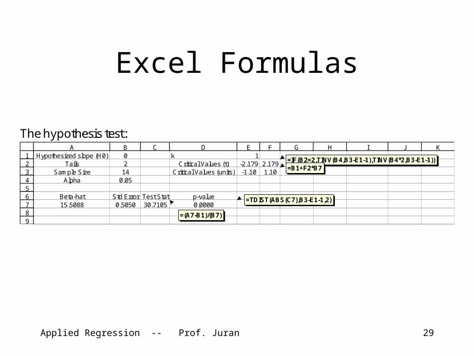
Excel Formulas
The hypothesis test:
123456789
A B C D E F G H I J KH ypothes ized s lope (H 0) 0 k 1
T a ils 2 C ritica l V a lues (t) -2 .179 2 .179S am ple S ize 14 C ritica l V a lues (un its ) -1 .10 1 .10
A lpha 0 .05
B eta -ha t S td E rro r T es t S ta t p -va lue15 .5088 0 .5050 30 .7105 0 .0000
=(A7-B 1)/(B 7)
= IF (B 2=2,T IN V (B 4,B 3-E 1-1),T IN V (B 4*2 ,B 3-E 1-1 ))=B 1+F 2*B 7
=T D IS T (AB S (C 7),B 3-E 1-1 ,2 )
Applied Regression -- Prof. Juran 30
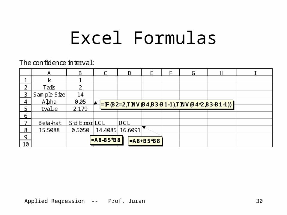
Excel FormulasThe confidence interval:
123456789
10
A B C D E F G H Ik 1
Tails 2Sample Size 14
Alpha 0.05t value 2.179
Beta-hat Std Error LCL UCL15.5088 0.5050 14.4085 16.6091
=A8-B5*B8 =A8+B5*B8
=IF(B2=2,TINV(B4,B3-B1-1),TINV(B4*2,B3-B1-1))
Applied Regression -- Prof. Juran 31
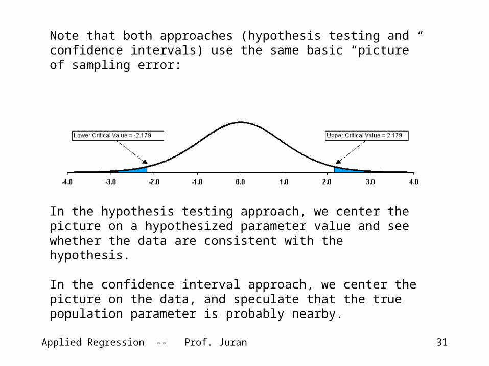
Note that both approaches (hypothesis testing and confidence intervals) use the same basic “picture” of sampling error:
In the hypothesis testing approach, we center the picture on a hypothesized parameter value and see whether the data are consistent with the hypothesis.
In the confidence interval approach, we center the picture on the data, and speculate that the true population parameter is probably nearby.
Applied Regression -- Prof. Juran 32
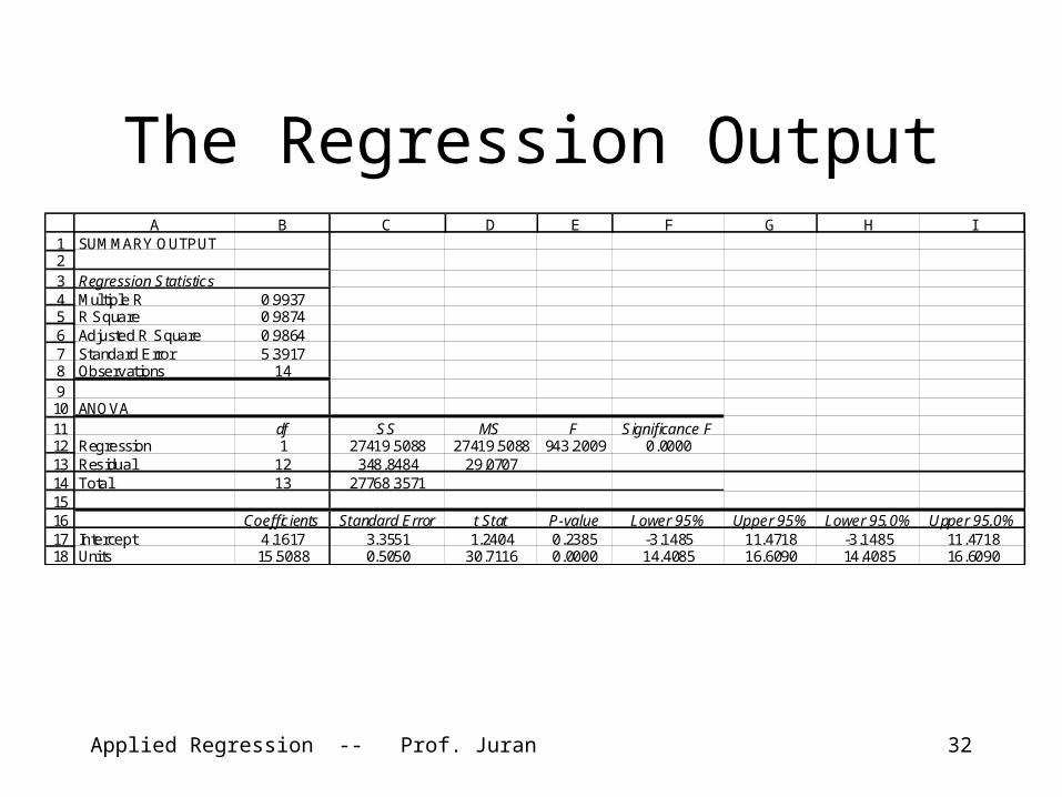
The Regression Output
123456789101112131415161718
A B C D E F G H ISUMMARY OUTPUT
Regression StatisticsMultiple R 0.9937R Square 0.9874Adjusted R Square 0.9864Standard Error 5.3917Observations 14
ANOVAdf SS MS F Significance F
Regression 1 27419.5088 27419.5088 943.2009 0.0000Residual 12 348.8484 29.0707Total 13 27768.3571
Coefficients Standard Error t Stat P-value Lower 95% Upper 95% Lower 95.0% Upper 95.0%Intercept 4.1617 3.3551 1.2404 0.2385 -3.1485 11.4718 -3.1485 11.4718Uni ts 15.5088 0.5050 30.7116 0.0000 14.4085 16.6090 14.4085 16.6090

Applied Regression -- Prof. Juran 33
Hypothesis Testing: Gardening Analogy
Rocks Dirt

Applied Regression -- Prof. Juran 34
Hypothesis Testing: Gardening Analogy

Applied Regression -- Prof. Juran 35
Hypothesis Testing: Gardening Analogy

Applied Regression -- Prof. Juran 36
Hypothesis Testing: Gardening Analogy
Applied Regression -- Prof. Juran 37
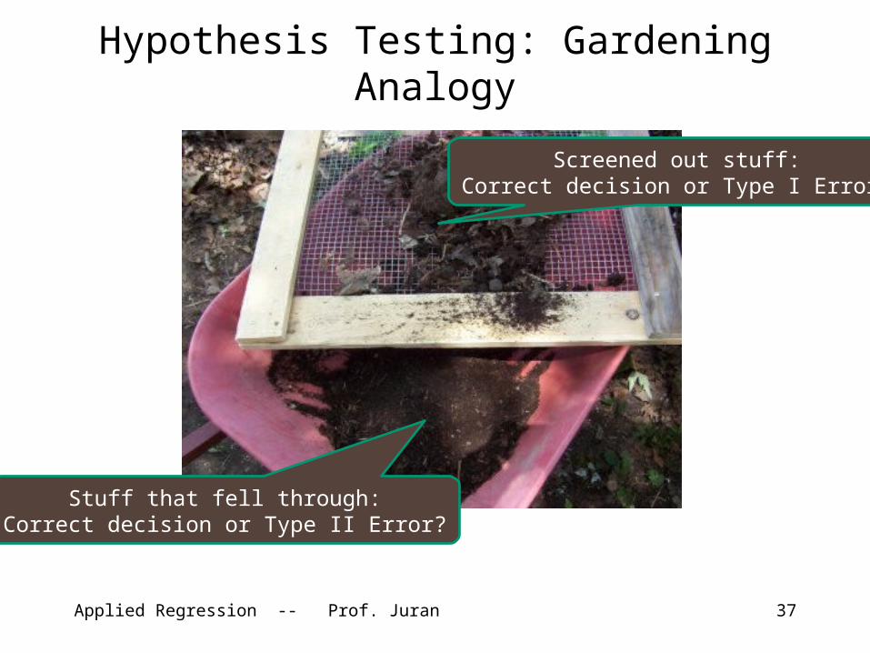
Hypothesis Testing: Gardening Analogy
Screened out stuff:Correct decision or Type I
Error?
Stuff that fell through:Correct decision or Type II
Error?

Applied Regression -- Prof. Juran 38
Stock BetasValue of $100 Invested Dec. 1, 1999
$-
$20
$40
$60
$80
$100
$120
$140
$160
$180
Nov-99 Feb-00 May-00 Aug-00 Nov-00 Feb-01 May-01 Aug-01 Nov-01 Feb-02 May-02 Aug-02 Nov-02 Feb-03 May-03 Aug-03 Nov-03 Feb-04 May-04
XOM
HPQ
AXP
GM
BEL
SPY
Applied Regression -- Prof. Juran 39
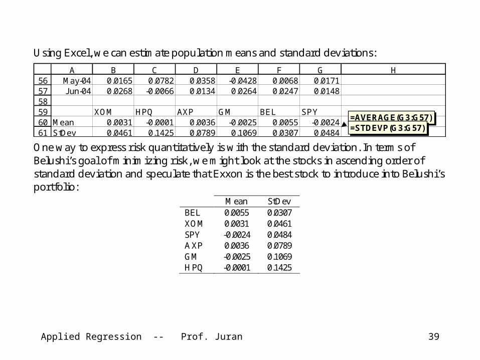
Using Excel, we can estimate population means and standard deviations:
565758596061
A B C D E F G HMay-04 0.0165 0.0782 0.0358 -0.0428 0.0068 0.0171Jun-04 0.0268 -0.0066 0.0134 0.0264 0.0247 0.0148
XOM HPQ AXP GM BEL SPYMean 0.0031 -0.0001 0.0036 -0.0025 0.0055 -0.0024StDev 0.0461 0.1425 0.0789 0.1069 0.0307 0.0484
=AVERAGE(G3:G57)=STDEVP(G3:G57)
One way to express risk quantitatively is with the standard deviation. In terms of Belushi’s goal of minimizing risk, we might look at the stocks in ascending order of standard deviation and speculate that Exxon is the best stock to introduce into Belushi’s portfolio:
Mean StDev BEL 0.0055 0.0307 XOM 0.0031 0.0461 SPY -0.0024 0.0484 AXP 0.0036 0.0789 GM -0.0025 0.1069 HPQ -0.0001 0.1425

Applied Regression -- Prof. Juran 40
ExxonMobil
0
5
10
15
20
25
30
35
40
-30% -25% -20% -15% -10% -5% 0% 5% 10% 15% 20% 25% 30% 35%
Monthly Returns
Freq
uen
cy
Hewlett-Packard
0
5
10
15
20
25
30
35
40
-30% -25% -20% -15% -10% -5% 0% 5% 10% 15% 20% 25% 30% 35%
Monthly Returns
Freq
uen
cy
American Express
0
5
10
15
20
25
30
35
40
-30% -25% -20% -15% -10% -5% 0% 5% 10% 15% 20% 25% 30% 35%
Monthly Returns
Freq
uen
cy
General Motors
0
5
10
15
20
25
30
35
40
-30% -25% -20% -15% -10% -5% 0% 5% 10% 15% 20% 25% 30% 35%
Monthly Returns
Freq
uen
cy
Belushi Portfolio
0
5
10
15
20
25
30
35
40
-30% -25% -20% -15% -10% -5% 0% 5% 10% 15% 20% 25% 30% 35%
Monthly Returns
Freq
uen
cy
S&P Exchange-Traded Fund
0
5
10
15
20
25
30
35
40
-30% -25% -20% -15% -10% -5% 0% 5% 10% 15% 20% 25% 30% 35%
Monthly Returns
Freq
uen
cy

Applied Regression -- Prof. Juran 41
We might also look at relationships between the stocks, looking for ones with a low correlation with Belushi’s portfolio.
XOM HPQ AXP GM BEL SPY XOM 1 HPQ -0.0856 1 AXP 0.4770 0.3589 1 GM 0.2677 0.3006 0.3862 1 BEL 0.4871 0.2697 0.5018 0.2253 1 SPY 0.3987 0.6520 0.6973 0.5190 0.6857 1
Correlations with Belushi portfolio, in ascending order: GM 0.2253 HPQ 0.2697 XOM 0.4871 AXP 0.5018
From these statistics, one might infer that Belushi’s best option is General Motors, or maybe Hewlett-Packard. This is in contrast to the inference we might have made from looking at standard deviations (where Exxon looked least risky).
Applied Regression -- Prof. Juran 42
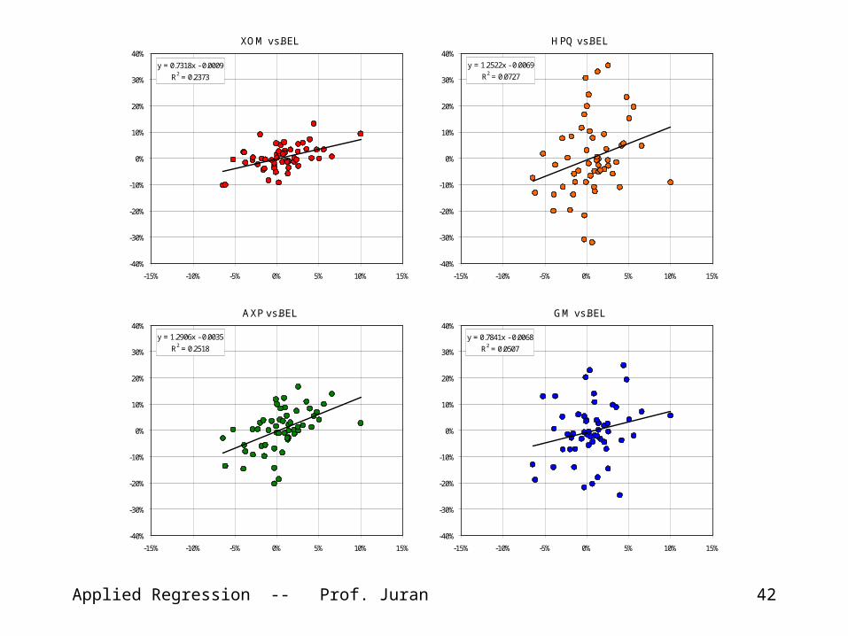
XOM vs.BEL
y = 0.7318x - 0.0009
R2 = 0.2373
-40%
-30%
-20%
-10%
0%
10%
20%
30%
40%
-15% -10% -5% 0% 5% 10% 15%
HPQ vs.BEL
y = 1.2522x - 0.0069
R2 = 0.0727
-40%
-30%
-20%
-10%
0%
10%
20%
30%
40%
-15% -10% -5% 0% 5% 10% 15%
AXP vs.BEL
y = 1.2906x - 0.0035
R2 = 0.2518
-40%
-30%
-20%
-10%
0%
10%
20%
30%
40%
-15% -10% -5% 0% 5% 10% 15%
GM vs.BEL
y = 0.7841x - 0.0068
R2 = 0.0507
-40%
-30%
-20%
-10%
0%
10%
20%
30%
40%
-15% -10% -5% 0% 5% 10% 15%

Applied Regression -- Prof. Juran 43
The relationship between beta and the other descriptive statistics (standard deviation and correlation) can seem counter-intuitive, as shown by these scatter diagrams using Belushi’s data:
Beta vs. StDev
0.0
0.2
0.4
0.6
0.8
1.0
1.2
1.4
0 0.02 0.04 0.06 0.08 0.1 0.12 0.14 0.16Standard Deviation
Bet
a (B
EL)
XOM
HPQ
AXP
GM
Beta vs. Correl
0.0
0.2
0.4
0.6
0.8
1.0
1.2
1.4
0.00 0.10 0.20 0.30 0.40 0.50 0.60Correlation (BEL)
Bet
a (B
EL)
XOM
HPQ
AXP
GM
Applied Regression -- Prof. Juran 44
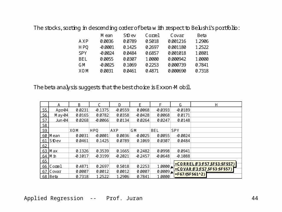
The stocks, sorting in descending order of beta with respect to Belushi’s portfolio: Mean StDev Correl Covar Beta AXP 0.0036 0.0789 0.5018 0.001216 1.2906 HPQ -0.0001 0.1425 0.2697 0.001180 1.2522 SPY -0.0024 0.0484 0.6857 0.001018 1.0801 BEL 0.0055 0.0307 1.0000 0.000942 1.0000 GM -0.0025 0.1069 0.2253 0.000739 0.7841 XOM 0.0031 0.0461 0.4871 0.000690 0.7318
The beta analysis suggests that the best choice is Exxon-Mobil.
5556575859606162636465666768
A B C D E F G HApr-04 0.0231 -0.1375 -0.0559 0.0068 -0.0393 -0.0189
May-04 0.0165 0.0782 0.0358 -0.0428 0.0068 0.0171Jun-04 0.0268 -0.0066 0.0134 0.0264 0.0247 0.0148
XOM HPQ AXP GM BEL SPYMean 0.0031 -0.0001 0.0036 -0.0025 0.0055 -0.0024StDev 0.0461 0.1425 0.0789 0.1069 0.0307 0.0484
Max 0.1326 0.3539 0.1665 0.2482 0.0998 0.0941Min -0.1017 -0.3199 -0.2021 -0.2457 -0.0648 -0.1088
Correl 0.4871 0.2697 0.5018 0.2253 1.0000Covar 0.0007 0.0012 0.0012 0.0007 0.0009Beta 0.7318 1.2522 1.2906 0.7841 1.0000
=CORREL(F3:F57,$F$3:$F$57)=COVAR(F3:F57,$F$3:$F$57)=F67/($F$61^2)
Applied Regression -- Prof. Juran 45
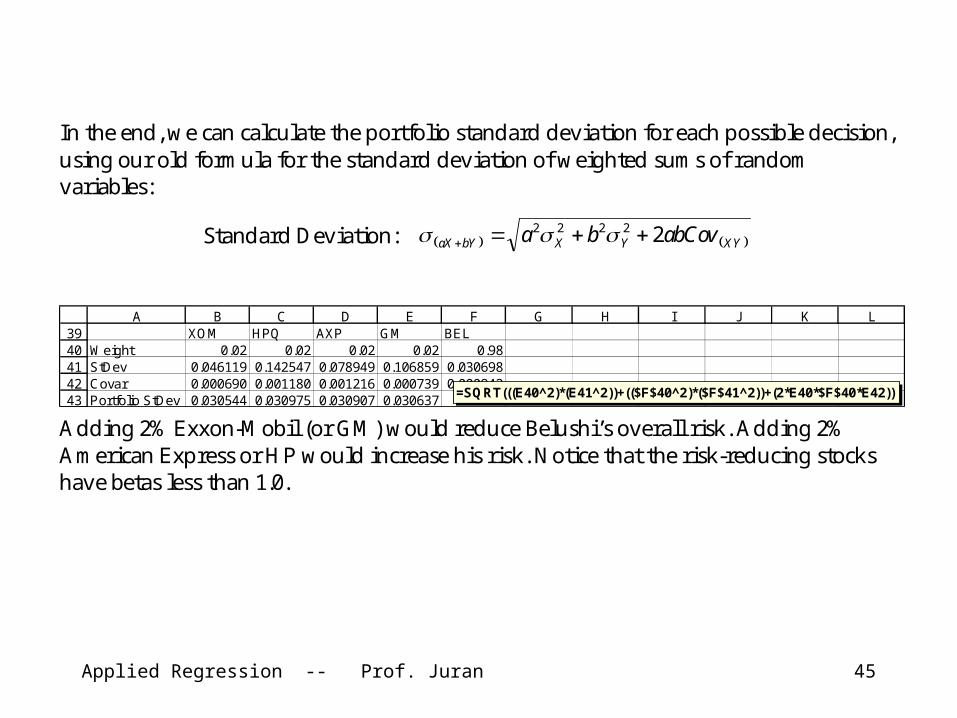
In the end, we can calculate the portfolio standard deviation for each possible decision, using our old formula for the standard deviation of weighted sums of random variables:
Standard Deviation: XYYXbYaX abCovba 22222
3940414243
A B C D E F G H I J K LXOM HPQ AXP GM BEL
Weight 0.02 0.02 0.02 0.02 0.98StDev 0.046119 0.142547 0.078949 0.106859 0.030698Covar 0.000690 0.001180 0.001216 0.000739 0.000942Portfolio StDev 0.030544 0.030975 0.030907 0.030637
=SQRT(((E40^2)*(E41^2))+(($F$40^2)*($F$41^2))+(2*E40*$F$40*E42)) Adding 2% Exxon-Mobil (or GM) would reduce Belushi’s overall risk. Adding 2% American Express or HP would increase his risk. Notice that the risk-reducing stocks have betas less than 1.0.
Applied Regression -- Prof. Juran 46
• More Simple Regression– Bottom Part of the Output
• Hypothesis Testing– Significance of the slope and
intercept parameters • Interval Estimation
– Confidence intervals for the slope and intercept parameters
Summary
Applied Regression -- Prof. Juran 47
For Sessions 3 & 4• Organize a Project Team • Review your regression notes from core
stats• Two cases:
– All-Around Movers– Manley’s Insurance