set 2: state-spaces and uninformed searchkkask/fall-2014 cs271/slides/02-state-space and... · set...

Set 2: State-spaces and Uninformed Search

ICS 271 Fall 2014

Kalev Kask

271-fall 2014

Problem-Solving Agents• Intelligent agents can solve problems by searching a state-space

• State-space Model– the agent’s model of the world – usually a set of discrete states– e.g., in driving, the states in the model could be towns/cities

• Goal State(s)– a goal is defined as a desirable state for an agent– there may be many states which satisfy the goal

• e.g., drive to a town with a ski-resort

– or just one state which satisfies the goal• e.g., drive to Mammoth

• Operators– operators are legal actions which the agent can take to move from

one state to another

271-fall 2014

Example: Romania

271-fall 2014

Example: Romania

• On holiday in Romania; currently in Arad.

• Flight leaves tomorrow from Bucharest

• Formulate goal:– be in Bucharest

• Formulate problem:– states: various cities

– actions: drive between cities

• Find solution:– sequence of actions (cities), e.g., Arad, Sibiu, Fagaras, Bucharest

271-fall 2014

Problem Types

• Static / Dynamic

Previous problem was static: no attention to changes in environment

• Observable / Partially Observable / Unobservable

Previous problem was observable: it knew its initial state.

• Deterministic / Stochastic

Previous problem was deterministic: no new percepts

were necessary, we can predict the future perfectly

• Discrete / continuous

Previous problem was discrete: we can enumerate all possibilities

271-fall 2014

A problem is defined by five items:

initial state e.g., "at Arad“

actions or successor function S(x) = set of action–state pairs – e.g., S(Arad) = {<Arad Zerind, Zerind>, … }

transition function – maps action X state state

goal test, (or goal state)e.g., x = "at Bucharest”, Checkmate(x)

path cost (additive)– e.g., sum of distances, number of actions executed, etc.– c(x,a,y) is the step cost, assumed to be ≥ 0

A solution is a sequence of actions leading from the initial state to a goal state

271-fall 2014

State-Space Problem Formulation

State-Space Problem Formulation

• A statement of a Search problem has 5 components

– 1. A start state S

– 2. A set of operators/actions which allow one to get from one state to another

– 3. transition function

– 4. A set of possible goal states G, or ways to test for goal states

– 5. Cost path

• A solution consists of

– a sequence of operators which transform S into a goal state G

• Representing real problems in a State-Space search framework

– may be many ways to represent states and operators

– key idea: represent only the relevant aspects of the problem (abstraction)

271-fall 2014

Abstraction/Modeling

• Definition of Abstraction:

• Navigation Example: how do we define states and operators?

– First step is to abstract “the big picture”

• i.e., solve a map problem

• nodes = cities, links = freeways/roads (a high-level description)

• this description is an abstraction of the real problem

– Can later worry about details like freeway onramps, refueling, etc

• Abstraction is critical for automated problem solving

– must create an approximate, simplified, model of the world for the computer to deal with: real-world is too detailed to model exactly

– good abstractions retain all important details

Process of removing irrelevant detail to create an abstract

representation: ``high-level”, ignores irrelevant details

271-fall 2014

Robot block world

• Given a set of blocks in a certain configuration,

• Move the blocks into a goal configuration.

• Example :

– (c,b,a) (b,c,a)

A

B

C

A

C

B

Move (x,y)

271-fall 2014

Operator Description

271-fall 2014

The State-Space Graph

• Problem formulation:

– Give an abstract description of states,

operators, initial state and goal state.

• Graphs:

– vertices, edges(arcs), directed arcs, paths

• State-space graphs:

– States are vertices

– operators are directed arcs

– solution is a path from start to goal

• Problem solving activity:

– Generate a part of the search space that contains a solution

State-space:

1. A set of states

2. A set of “operators”/transitions

3. A start state S

4. A set of possible goal states

5. Cost path

271-fall 2014

The Traveling Salesperson Problem• Find the shortest tour that visits all cities without

visiting any city twice and return to starting point.• State:

– sequence of cities visited

• S0 = AC

DA

E

F

B

271-fall 2014

The Traveling Salesperson Problem• Find the shortest tour that visits all cities without

visiting any city twice and return to starting point.

• State: sequence of cities visited

• S0 = A

},,{ dca },,|),,,{( dcaXxdca

• Solution = a complete tour

C

DA

E

F

B

Transition model

271-fall 2014

Example: 8-queen problem

271-fall 2014

Example: 8-Queens

• states? -any arrangement of n<=8 queens

-or arrangements of n<=8 queens in leftmost n columns, 1 per column, such that no queen attacks any other.

• initial state? no queens on the board

• actions? -add queen to any empty column

-or add queen to leftmost empty column such that it is not attacked by other queens.

• goal test? 8 queens on the board, none attacked.

• path cost? 1 per move

271-fall 2014

The Sliding Tile Problem

),,( zlocylocxmove Up

Down

Left

Right

271-fall 2014

The “8-Puzzle” Problem

1 2 3

4

8

6

7 5

1 2 3

4 5 6

7 8

Goal State

Start State

1 2 3

4

8

6

7

5

Example: robotic assembly

• states?: real-valued coordinates of robot joint angles parts of the object to be assembled

• actions?: continuous motions of robot joints• goal test?: complete assembly• path cost?: time to execute

new271-fall 2014

Formulating Problems;Another Angle

• Problem types

– Satisfying: 8-queen

– Optimizing: Traveling salesperson

• Goal types

– board configuration

– sequence of moves

– A strategy (contingency plan)

• Satisfying leads to optimizing since “small is quick”

• For traveling salesperson

– satisfying easy, optimizing hard

• Semi-optimizing:

– Find a good solution

• In Russel and Norvig:

– single-state, multiple states, contingency plans, exploration problems

271-fall 2014

Searching the State Space

• States, operators, control strategies

• The search space graph is implicit

• The control strategy generates a small search tree.

• Systematic search

– Do not leave any stone unturned

• Efficiency

– Do not turn any stone more than once

271-fall 2014

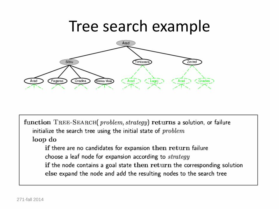
Tree search example

271-fall 2014

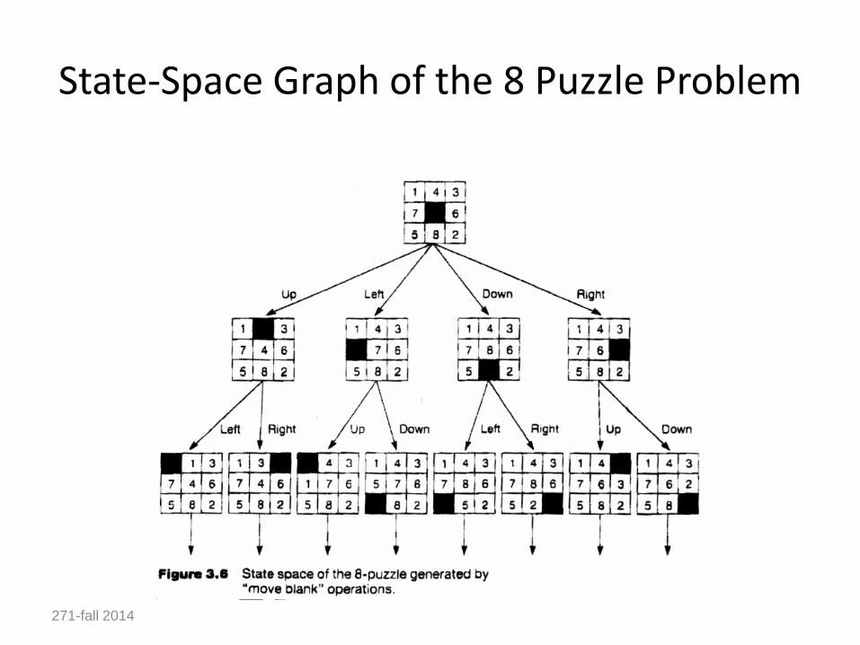
State-Space Graph of the 8 Puzzle Problem

271-fall 2014

Implementation

• States vs Nodes– A state is a (representation of) a physical configuration– A node is a data structure constituting part of a search tree contains info

such as: state, parent node, action, path cost g(x), depth

• The Expand function creates new nodes, filling in the various fields and using the SuccessorFn of the problem to create the corresponding states.

• Queue managing frontier :– FIFO– LIFO– priority

271-fall 2014

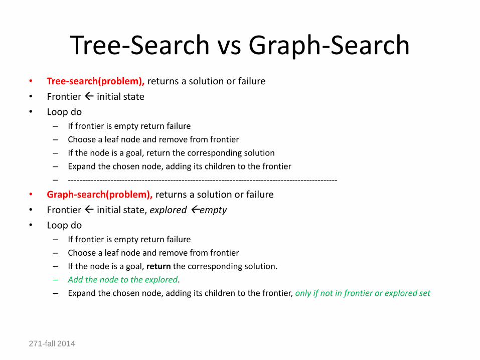
Tree-Search vs Graph-Search• Tree-search(problem), returns a solution or failure

• Frontier initial state

• Loop do

– If frontier is empty return failure

– Choose a leaf node and remove from frontier

– If the node is a goal, return the corresponding solution

– Expand the chosen node, adding its children to the frontier

– -----------------------------------------------------------------------------------------------

• Graph-search(problem), returns a solution or failure

• Frontier initial state, explored empty

• Loop do

– If frontier is empty return failure

– Choose a leaf node and remove from frontier

– If the node is a goal, return the corresponding solution.

– Add the node to the explored.

– Expand the chosen node, adding its children to the frontier, only if not in frontier or explored set

271-fall 2014

Tree-Search vs. Graph-Search• Example : Assemble 5 objects {a, b, c, d, e}

• A state is a bit-vector (length 5), 1=object in assembly

• 11010 = a, b, d in assembly, c, e not

• State space

– number of states 25 = 32

– number of edges (25)∙5∙½ = 80

• Tree-search space

– number of nodes 5! = 120

• State can be reached in multiple ways

– 11010 can be reached a+b+d or a+d+b etc.

• Graph-search :

– three kinds of nodes : unexplored, frontier, explored

– before adding a node, check if a state is in frontier or explored set

271-fall 2014

Graph-Search

271-fall 2014

Why Search Can be Difficult

• At the start of the search, the search algorithm does not know

– the size of the tree

– the shape of the tree

– the depth of the goal states

• How big can a search tree be?

– say there is a constant branching factor b

– and one goal exists at depth d

– search tree which includes a goal can havebd different branches in the tree (worst case)

• Examples:

– b = 2, d = 10: bd = 210= 1024

– b = 10, d = 10: bd = 1010= 10,000,000,000

271-fall 2014

Searching the Search Space

• Uninformed (Blind) search– Breadth-first– Uniform-Cost first– Depth-first– Iterative deepening depth-first– Bidirectional– Depth-First Branch and Bound

• Informed Heuristic search – Greedy search, hill climbing, Heuristics

• Important concepts:– Completeness– Time complexity– Space complexity– Quality of solution

271-fall 2014

Breadth-First Search• Expand shallowest unexpanded node

• Frontier: nodes waiting in a queue to be explored, also called OPEN

• Implementation:

– frontier is a first-in-first-out (FIFO) queue, i.e., new successors go at end of the queue.

Is A a goal state?

271-fall 2014

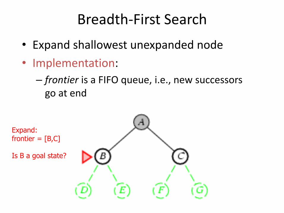
Breadth-First Search

• Expand shallowest unexpanded node

• Implementation:

– frontier is a FIFO queue, i.e., new successors go at end

Expand:frontier = [B,C]

Is B a goal state?



• Implementation:


Expand:frontier=[C,D,E]

Is C a goal state?

271-fall 2014



• Implementation:


Expand:frontier=[D,E,F,G]

Is D a goal state?

271-fall 2014


271-fall 2014

Actually, in BFS we

can check if a node

is a goal node when it is

generated (rather than expanded)

Breadth-First-Search (*)

• 1. Put the start node s on OPEN

• 2. If OPEN is empty exit with failure.

• 3. Remove the first node n from OPEN and place it on CLOSED.

• 4. Expand n, generating all its successors.

– If child is not in CLOSED or OPEN, then

– If child is not a goal, then put them at the end of OPEN in some order.

• 5. If n is a goal node, exit successfully with the solution obtained by tracing back pointers

from n to s.

• Go to step 2.

* This is graph-search

OPEN = frontier, CLOSED = explored

271-fall 2014

Example: Map Navigation

S G

A B

D E

C

F

S = start, G = goal, other nodes = intermediate states, links = legal transitions

271-fall 2014

Initial BFS Search TreeS

A D

B D

C E

Note: this is the search tree at some particular point in

in the search.

S G

A B

D E

C

F

E

Not expanded

By graph-search

271-fall 2014

A

Complexity of Breadth-First Search

• Time Complexity

– assume (worst case) that there is 1

goal leaf at the RHS

– so BFS will expand all nodes

= 1 + b + b2+ ......... + bd

= O (bd)

• Space Complexity

– how many nodes can be in the queue

(worst-case)?

– at depth d there are bd unexpanded

nodes in the Q = O (bd)

d=0

d=1

d=2

d=0

d=1

d=2

G

G

271-fall 2014

Examples of Time and Memory Requirements for Breadth-First Search

Depth of Nodes

Solution Expanded Time Memory

0 1 1 millisecond 100 bytes

2 111 0.1 seconds 11 kbytes

4 11,111 11 seconds 1 megabyte

8 108 31 hours 11 giabytes

12 1012 35 years 111 terabytes

Assuming b=10, 1000 nodes/sec, 100 bytes/node

271-fall 2014

Breadth-First Search (BFS) Properties• Solution Length: optimal• Expand each node once (can check for duplicates,

performs graph-search)• Search Time: O(bd)• Memory Required: O(bd)• Drawback: requires exponential space

1

3

7

15141312111098

4 5 6

2

271-fall 2014

Uniform Cost Search• Expand lowest-cost OPEN node (g(n))

• In BFS g(n) = depth(n)

Requirement

g(successor)(n)) g(n)271-fall 2014

Uniform cost search 1. Put the start node s on OPEN

2. If OPEN is empty exit with failure.

3. Remove the first node n from OPEN and place it on CLOSED.

4. If n is a goal node, exit successfully with the solution obtained by tracing back pointers from n to s.

5. Otherwise, expand n, generating all its successors attach to them pointers back to n, and put them in OPEN in order of shortest cost

6. Go to step 2.

DFS Branch and Bound

At step 4: compute the cost of the solution found and update the upper bound U.

at step 5: expand n, generating all its successors attach to them

pointers back to n, and put on top of OPEN.

Compute cost of partial path to node and prune if larger than U.

.271-fall 2014

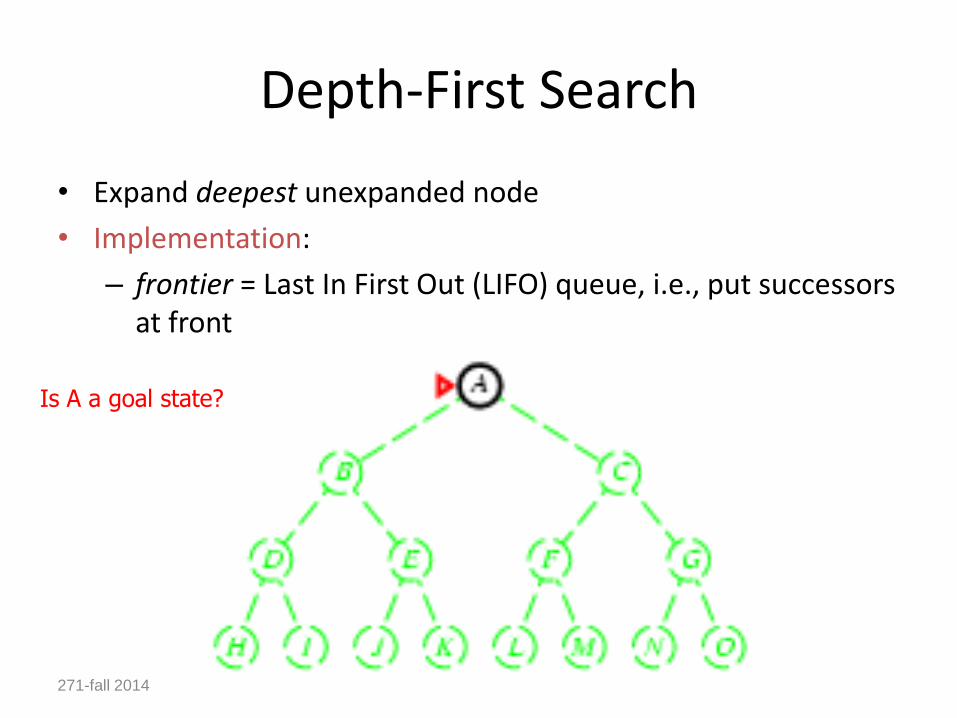
Depth-First Search

• Expand deepest unexpanded node

• Implementation:

– frontier = Last In First Out (LIFO) queue, i.e., put successors at front

Is A a goal state?

271-fall 2014

Depth-first search


• Implementation:

– frontier = LIFO queue, i.e., put successors at front

queue=[B,C]

Is B a goal state?

271-fall 2014

Depth-first search


• Implementation:


queue=[D,E,C]

Is D = goal state?

271-fall 2014

Depth-first search


• Implementation:


queue=[H,I,E,C]

Is H = goal state?

271-fall 2014

Depth-first search


• Implementation:


queue=[I,E,C]

Is I = goal state?

271-fall 2014

Depth-first search


• Implementation:


queue=[E,C]

Is E = goal state?

271-fall 2014

Depth-first search


• Implementation:


queue=[J,K,C]

Is J = goal state?

271-fall 2014

Depth-first search


• Implementation:


queue=[K,C]

Is K = goal state?

271-fall 2014

Depth-first search


• Implementation:


queue=[C]

Is C = goal state?

271-fall 2014

Depth-first search


• Implementation:


queue=[F,G]

Is F = goal state?

271-fall 2014

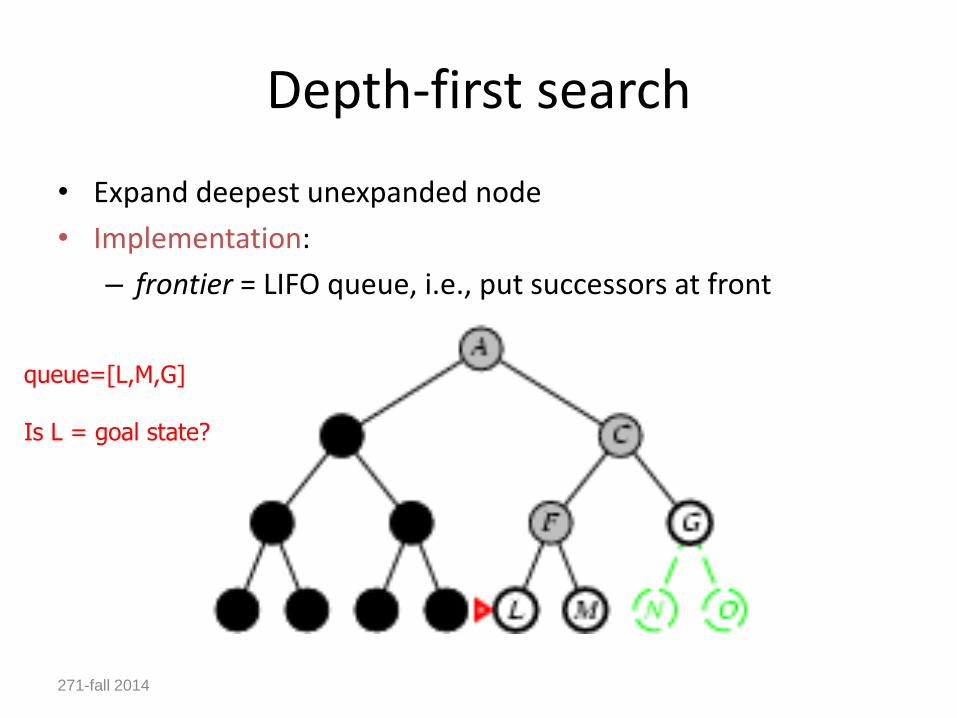
Depth-first search


• Implementation:


queue=[L,M,G]

Is L = goal state?

271-fall 2014

Depth-first search


• Implementation:


queue=[M,G]

Is M = goal state?

271-fall 2014

Depth-First Search (DFS)

S

A

B

D

C E

D

D

F

G

Here, (if tree-search) then to avoid

infinite depth (in case of finite

state-space graph) assume we

don’t expand any child node which

appears already in the path from

the root S to the parent. (Again,

one could use other strategies)

S G

A B

D E

C

F

271-fall 2014

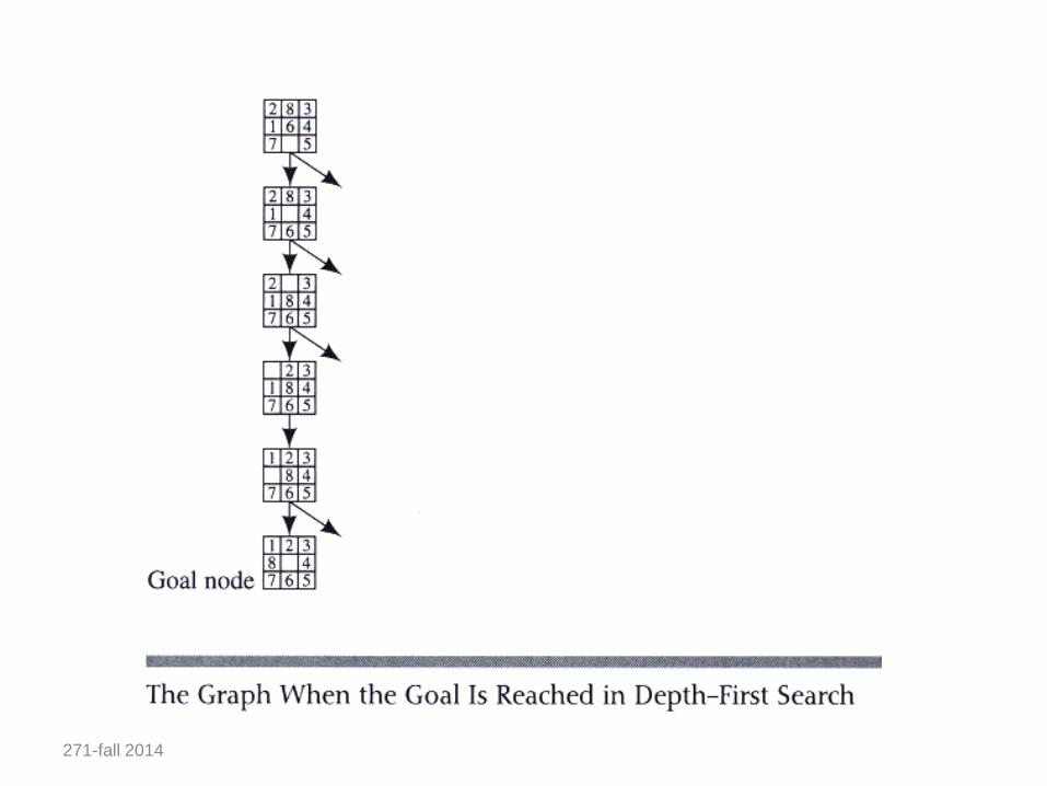
Depth-First Search

271-fall 2014

271-fall 2014

Depth-First-Search (*)

1. Put the start node s on OPEN

2. If OPEN is empty exit with failure.

3. Remove the first node n from OPEN.

4. If n is a goal node, exit successfully with the solution obtained by tracing back pointers from n to s.

5. Otherwise, expand n, generating all its successors (check for self-loops)attach to them pointers back to n,

and put them at the top of OPEN in some order.

6. Go to step 2.

*search the tree search-space (but avoid self-loops)

** the default assumption is that DFS searches the underlying search-tree

271-fall 2014

Complexity of Depth-First Search?• Time Complexity

– assume d is deepest path in the search space

– assume (worst case) that there is 1 goal leaf at the RHS

– so DFS will expand all nodes

=1 + b + b2+ ......... + bd

= O (bd)

• Space Complexity (for tree-search)– how many nodes can be in the

queue (worst-case)?– O(bd) if deepest node at

depth d

d=0

d=1

d=2

G

d=0

d=1

d=2

d=3

d=4

271-fall 2014

Example, Diamond Networksgraph-search vs tree-search (BFS vs DFS)

271-fall 2014

• Graph-search & BFS

• Tree-search & DFS

Depth-First tree-search Properties

• Non-optimal solution path

• Incomplete unless there is a depth bound

• (we will assume depth-limited DF-search)

• Re-expansion of nodes (when the state-space is a graph)

• Exponential time

• Linear space (for tree-search)

271-fall 2014

Comparing DFS and BFS

• BFS optimal, DFS is not• Time Complexity worse-case is the same, but

– In the worst-case BFS is always better than DFS– Sometime, on the average DFS is better if:

• many goals, no loops and no infinite paths

• BFS is much worse memory-wise• DFS can be linear space• BFS may store the whole search space.

• In general• BFS is better if goal is not deep, if long paths, if many loops, if

small search space• DFS is better if many goals, not many loops• DFS is much better in terms of memory

271-fall 2014

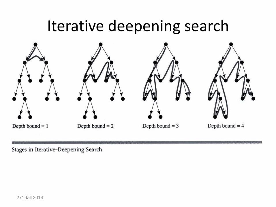
Iterative-Deepening Search (DFS)

• Every iteration is a DFS with a depth cutoff.

Iterative deepening (ID)1. i = 1

2. While no solution, do

3. DFS from initial state S0 with cutoff i

4. If found goal, stop and return solution, else, increment cutoff

Comments:

• IDS implements BFS with DFS

• Only one path in memory

• BFS at step i may need to keep 2i nodes in OPEN

271-fall 2014

Iterative deepening search L=0

271-fall 2014


271-fall 2014

Iterative Deepening Search L=3

271-fall 2014

Iterative deepening search

271-fall 2014

Iterative Deepening (DFS)• Time:

)(2)1(

2

11

11

)( nbO

b

nbn

jb

jbnT

BFS time is O(bn), b is the branching degree

IDS is asymptotically like BFS,

For b=10 d=5 d=cut-off

DFS = 1+10+100,…,=111,111

IDS = 123,456

Ratio is1b

b

271-fall 2014

Summary on IDS

• A useful practical method

– combines

• guarantee of finding an optimal solution if one exists (as in BFS)

• space efficiency, O(bd) of DFS

• But still has problems with loops like DFS

271-fall 2014

Bidirectional Search

• Idea– simultaneously search forward from S and backwards from G– stop when both “meet in the middle”– need to keep track of the intersection of 2 open sets of nodes

• What does searching backwards from G mean– need a way to specify the predecessors of G

• this can be difficult, • e.g., predecessors of checkmate in chess?

– what if there are multiple goal states?– what if there is only a goal test, no explicit list?

• Complexity– time complexity is best: O(2 b(d/2)) = O(b (d/2))– memory complexity is the same

271-fall 2014

Bi-Directional Search

271-fall 2014

Comparison of Algorithms

271-fall 2014

Summary• A review of search

– a search space consists of nodes and operators: it is a tree/graph

• There are various strategies for “uninformed search”

– breadth-first

– depth-first

– iterative deepening

– bidirectional search

– Uniform cost search

– Depth-first branch and bound

• Repeated states can lead to infinitely large search trees

– we looked at methods for detecting repeated states

• All of the search techniques so far are “blind” in that they do not look at how far away the goal may be: next we will look at informed or heuristic search, which directly tries to minimize the distance to the goal.

271-fall 2014

set 2: state-spaces and uninformed searchkkask/fall-2014 cs271/slides/02-state-space and... · set...

Documents