sex and credit: is there a gender bias in...
TRANSCRIPT

Sex and Credit: Is There a Gender Bias in Lending?
Thorsten Beck♣ CentER, Dept. of Economics, Tilburg University and CEPR
Patrick Behr#
EBAPE, Fundacao Getulio Vargas
Andreas Madestam∗ IGIER and Department of economics, Bocconi University
This version: January 2012
Abstract This paper examines the effects of group identity in the credit market. Exploiting the quasi-random assignment of first-time borrowers to loan officers of a large Albanian lender, we test for own-gender bias in the loan officer-borrower match. We find that borrowers pay, on average, 28 basis points higher interest rates when paired with a loan officer of the other sex. The results indicate the presence of a taste-based rather than a statistical bias, as borrowers’ likelihood of going into arrears is independent of loan officer gender. Ending up with an opposite-sex loan officer also affects demand for credit, with borrowers being 11 percent less likely to return for a second loan. The evidence further suggests that the bias originates with both female and male loan officers. The bias is more pronounced when the social distance, as proxied by difference in age between the loan officer and the borrower, increases and when financial market competition declines. This is consistent with theories that predict a taste-based bias to be stronger when the psychological costs of being biased are lower and the discretion in setting interest rates is higher. Together our results show that own-gender preferences can have substantial welfare effects.
JEL Classification: G21, G32, J16. Keywords: Identity, interest rates, gender, loan officers, microfinance.
♣ Department of Economics and European Banking Center, Tilburg University, P.O. Box 90153, 5000 LE Tilburg, The Netherlands, and CEPR, Email: [email protected]. # Brazilian School of Public and Business Administration, Fundacao Getulio Vargas, Praia de Botafogo 190, 22253-900 Rio de Janeiro, Brazil, [email protected] (corresponding author). ∗ IGIER and Department of Economics, Bocconi University, Via Roentgen 1, 20136 Milan, Italy, Email: [email protected]. We are grateful to Santosh Anagol, Tore Ellingsen, Marcel Fafchamps, Steven Poelhekke, Raghuram Rajan, David Yanagizawa-Drott, and seminar participants at Goethe University Frankfurt, the NEUDC 2011 at Yale, Stockholm School of Economics, Tilburg University, the Development Economics Workshop in Bergen 2010, and University of Göttingen. This paper was previously circulated under the title ” Sex and Credit: Is There a Gender Bias in Microfinance?”

2
1 Introduction
Group identity in the form of family, ethnicity, and gender is a powerful predictor of social
preferences (Akerlof and Kranton, 2000; Chen and Li, 2009; Benjamin et al., 2010). In
particular, people generally favor in-group over out-group members. Favoritism based on, for
example, gender identity can lead to inefficient transactions and/or lost opportunities.
However, gender similarity may also entail trust, reciprocity, and efficiency due to shared
norms and understandings. In this paper, we examine one important form of group identity,
gender, and the consequences of own-gender preferences for outcomes in the credit market.
Credit transactions rely heavily on the interaction between loan officers and
borrowers. Microcredit is a case in point, with most clients being small and opaque, leaving
the lending decision at the discretion of the loan officer. If bank officers and borrowers share
gender identity, this could improve efficiency through a better understanding of the clients’
particular circumstances. For example, female loan officers may better appreciate the ability
of female entrepreneurs in terms of completing their project and/or repaying the debt.
Conversely, a gender bias can also generate unfair pricing. While access to formal sources of
credit is often described as the main obstacle for the poor, the typically high interest rates for
microloans can be a deterrence factor too. Recent work shows that poor borrowers are very
sensitive to small changes in interest rates (Karlan and Zinman, 2008). If a gender bias in the
relationship between loan officers and borrowers results in higher interest rates, this may have
negative repercussions not only for the cost of credit, but also for take up of loans by poor
borrowers.
Using a large dataset of loan transactions from a microcredit lender in Albania, we
study if there is a bias against borrowers of the opposite gender by their respective loan
officer and the consequences of this bias for take up of loans. In particular, we assess if
borrowers pay higher interest rates when matched with an opposite-sex loan officer and

3
whether the bias has an effect on the take up of additional loans from the same lender. As our
data include information on both the price and the loan performance in terms of arrears, we
are able to distinguish between statistical bias (Phelps, 1972; Arrow, 1973), which implies
higher interest rates for riskier borrowers, and taste-based bias or prejudice (Becker, 1957),
which implies higher interest rates independent of the level of riskiness. A better
understanding of which type of bias is operative has important implications for policy.
Prejudice, being inconsistent with profit maximization, should motivate policymakers to
promote competition-enhancing strategies as well as anti-discrimination literacy programs.
Statistical bias, often consistent with profit maximization, should motivate policymakers to
consider other policies to support disadvantaged minorities.
Estimating the effect of own-gender preferences presents two main challenges. First, if
male or female borrowers with certain characteristics are more likely to be assigned the same
or opposite-sex loan officers, the true effect of loan officer gender would be biased. Second, if
unobserved borrower traits are correlated with borrower gender, and if these can be observed
by the loan officers but not by the researchers, it is not clear whether a significant coefficient
on gender is due to a loan officer bias or the unobservable traits.
We address these issues by exploiting a random component of the institutional setting:
the fact that first-time borrowers are arbitrarily assigned to their respective loan officer, with
the sector of activity being the only factor driving assignment to a specific officer.
Conditional on sector, the random assignment of borrowers to loan officers ensures that the
unobservable borrower characteristics are the same across all loan officers, regardless of loan
officer gender. In particular, we employ a difference-in-differences strategy and compare the
difference in outcomes (for example, the interest rate) for male and female borrowers

4
obtaining a loan from a male loan officer to the difference between male and female
borrowers obtaining a loan from a female loan officer.1
Our estimates provide convincing evidence of an own-gender preference, with
important repercussions for subsequent loan demand.2 Specifically, borrowers assigned to
loan officers of the opposite rather than their own sex pay on average 28 basis points higher
interest rates. In addition, there is no evidence that the loan officer-borrower gender match
predicts the likelihood of falling into arrears, allowing us to distinguish between taste-based
and statistical bias. If borrowers paying a higher interest rate were more likely to fall into
arrears, this would indicate a statistical bias. As this is not the case, our results imply a loan
officer-specific taste for gender bias: loan officers charge higher interest rates to borrowers of
the other gender although there is no difference in ex-post riskiness (or arrear probability).
Ending up with an opposite-sex loan officer also has a significant impact on take up of
loans. First-time borrowers matched with a loan officer of the opposite gender and who,
consequently, had to pay higher interest rates, are 6.4 percentage points less likely to return
for a second loan. Given that 60 percent of the borrowers return to the same lender for a
second loan, this is equivalent of a 10.6 percent decrease, a substantial economic effect. On
top of paying higher interest rates on their first loans, there is thus a negative impact on the
demand for credit. In addition, the negative effect of being matched with an opposite-sex loan
officer is stronger in smaller branches, as measured by the number of loan officers employed
per branch office, for borrowers with no personal guarantee, and for borrowers of small loan
amounts. A possible interpretation is that smaller branches leave borrowers fewer options to
find alternative loan officers, as the likelihood of being matched with the same opposite-sex
loan officer is higher when returning for a second loan. Similarly, borrowers without personal 1 The identifying assumption of the difference-in-differences estimator requires that the unobservable characteristics are the same in the two differences. 2 While this may be due to either male or female (or both) favoring borrowers of their own gender, or disfavoring those of the other gender, we provide suggestive evidence that the bias stems from own-gender preferences for both female and male loan officers.

5
guarantees from another client of the financial institution have less personal connection to the
lender. Finally, borrowers of small amounts are more likely to satisfy their lending needs from
another financial institution.
To better understand some of the possible mechanisms driving the taste-based bias, we
examine heterogeneous outcomes related to our findings. We show that the effect on the
interest rate partially can be explained by loan officer and borrower age. In particular, loan
officers younger than the median (loan officer age) charge higher interest rates when matched
with an opposite-sex borrower. Meanwhile, above median-aged borrowers pay higher interest
rates when interacting with a loan officer of the opposite gender. One interpretation of these
results is the concept of social distance. Consistent with studies of cognitive behavior, there is
a psychological cost involved in being biased that increases in cases where it is easier for the
biased party to relate to the individual being biased against (Goodwin et al., 2000; Blair,
2002). For example, a male loan officer may have stereotype beliefs about women. However,
if he interacts with a female borrower of similar age, he is more likely to identify with her
and, hence, experience a higher cost coming from the bias. Meanwhile, mistreating someone
of the opposite sex that is older (and, hence, quite different) could be associated with a
smaller loss of utility.
A second, complementary, mechanism is that the bias is more pronounced in
situations when loan officers have additional discretion in setting interest rates. Specifically,
we measure discretion in terms of competition from other financial institutions. While low
competition per se has a statistically insignificant (although positive) effect on the bias, it has
a substantial impact once we focus on below-median aged loan officers. The bias is stronger
for this category of loan officers when there is less competition. This is consistent with

6
theories predicting that competition can erode a taste-based bias. For instance, Becker (1957)
argues that discrimination is costly and harder to sustain in competitive environments.3
Taken together, the results indicate that loan officers’ own-gender preferences have
non-trivial welfare effects for opposite-sex consumers (higher interest rates and lower take
up) and providers of credit (lower long-run profits through diminished demand in the
opposite-gender matches).4 When exploring whether the bias stems from male loan officers
taking action toward female borrowers or from female loan officers toward male borrowers,
we find that officers of both gender engage in interest setting biases. Similarly, female and
male loan officers are equally likely to have an adverse effect on take-up rates of opposite-sex
borrowers.
This paper speaks to several literatures. First, while there is no research explicitly
examining the existence of a gender bias in microfinance, Karlan and Zinman’s (2008) study
is especially relevant for the present analysis. Using experimental field data from a South
African lender, where the interest rate offers were randomized, Karlan and Zinman show that
clients were sensitive to interest rate changes, in particular to increases in price above the
lender’s standard rates. In light of the interest rate differential identified in our paper, Karlan
and Zinman’s finding suggests that a gender bias-induced price gap may have important
effects on credit take up. This is indeed what we find.
Second, our paper also contributes to the empirical literature examining poor peoples’
barriers to credit by identifying the existence of asymmetric information in the credit market
(Karlan and Zinman, 2009). It further links to the work looking at mechanisms that can
3 In a developed-country setting, Black and Strahan (2001) and Levine et al. (2010) also find that discrimination against female and minority-race employees fell in the U.S. after a branch deregulation resulted in higher competition. 4 Unfortunately, our data do not allow us to construct precise measures of short-term profits because the bank does not collect the necessary information on actual repayments, the exact cost per loan, or the loan recoveries in case a loan defaults. Also, we would not be able to trace any recovered amounts back to the loan officers in our dataset, since the loan responsibility switches to a special loan recovery department once a loan is in arrears for more than 60 days. In addition, we do not have information about the gender of the individuals working in the loan recovery department.
7
improve access to finance, such as social capital (Karlan, 2007; Feigenberg et al., 2011) and
joint liability (Giné and Karlan, 2011). The setting of the current study, a for-profit lender in
Albania, extending credit under individual liability also fits the pattern of the second
generation of microcredit (Armendáriz and Morduch, 2005; Karlan and Morduch, 2009)
which has evolved in the direction of more traditional retail and small business lending.
Third, while there are studies looking at own-race preferences in police behavior
(Donohue and Levitt, 2001), in judicial sentencing (Welch et al., 1988) in the workplace
(Stoll et al., 2004), and in sports (Price and Wolfers, 2010; Parsons et al., 2011), our paper is
the first that seeks to account for an own-gender bias in lending. More generally, there is a
literature documenting biases in credit markets, predominately using U.S. data on either
mortgage (Munnell et al., 1996; Berkovec et al., 1998; Ladd, 1998; Ross and Yinger, 2002;
Han, 2004) or small business lending (Cavalluzzo and Cavalluzzo, 1998; Blanchflower et al.,
2003, Blanchard et al., 2008; Bellucci et al., 2010).5 While these studies on minority or
gender bias have their merit, they suffer from two main shortcomings. First, as both statistical
and taste-based bias can imply higher rejection rates for minority clients, it is often not clear
what type of bias is being identified (see Berkovec et al., 1998 and Han, 2004 for exceptions
though).6 Second, and more importantly, existing work does not contain all the characteristics
that lenders observe when approving the loans and setting the contract terms. Hence, one can
never be sure that the loan applicants being compared are truly similar from the loan officers’
perspective. As a consequence, any measured differences in outcomes could be attributed to
these factors unobserved by the researcher. Using the quasi-random assignment of borrowers
to loan officers in our sample allows us to address these shortcomings. Our dataset also
permits for a cleaner test of an interest rate gap across borrower gender as we have
5 For a survey of this literature, see Bellucci et al. (2010). 6 Becker (1993) writes (referring to influential work by the Federal Reserve Bank of Boston [Munnell et al., 1996]) that studies trying to identify a gender bias require examining not only credit denial, but also the default, interest charges, late payments, and other determinants of the loans profitability.

8
information on loan performance.7 Moreover, previous work does not combine supply and
demand-side analysis, that is, the effect of the gender bias on take up of financial services.
Finally, this paper fits into a small but growing literature examining the importance of
loan officers in lending stressing long-term relationships, compensation schemes, loan officer
rotation, and loan officer gender for loan performance (Agarwal and Wang, 2009; Hertzberg
et al., 2010; Beck et al., 2011; Drexler and Schoar, 2011).
In the next section we provide institutional background information about our lender
and the loan process, outline our methodology, and describe the data. Section three presents
the main empirical results, while section four explores different mechanisms that help
interpret our results. Section five concludes.
2 Data and identification strategy
This section provides background information about the lender, our identification strategy, as
well as a first look at the data, including descriptive statistics.
2.1 Institutional background information
We use loan-level data from a large for-profit commercial lender serving individuals and
small- and medium-sized enterprises in Albania. The dataset includes nearly 8,000 loans
given by the lender over the period January 1996 to December 2006. In addition, our data
contains information on 279 loan officers and covers 21 branches of the bank.8 While the
lender clearly focuses on the low-income and microenterprise segment, financial
sustainability and therefore profitability is its primary goal. 7 This is of particular importance as variation in interest rates may simply be driven by different degrees of risk associated with loans given to borrowers of the same or opposite gender that materialize ex-post. Though we are able to measure only ex-post risk, and borrowers’ risk behavior can be influenced by the interest rate, this would actually bias our estimations towards finding a higher arrear probability among borrowers matched to loan officers of the other gender. 8 For most loan officers, this is the first formal job after college. Male loan officers are, on average, two years older at entry since they have to undergo military service of two years.

9
Loan officers working for this lender have discretion on the rejection and approval of
a loan application as well as setting the interest rate. The loan officer that originates a certain
loan is also in charge of monitoring the repayment behavior of the borrower. If a loan is in
arrears for more than 30 days, the loan officer intensifies monitoring, for instance, by calling
or visiting the borrower to inquire about the reasons for repayment delay. When a loan is in
arrears for more than 60 days, it is transferred to a special loan recovery department and, thus,
a new loan officer. We can therefore follow the relationship between a borrower and loan
officer from approval over loan condition setting to its performance in terms of arrears up to
60 days, but not beyond that point in time as we lack information about the gender of the loan
officers working in the loan recovery department.
Assignment of borrowers to loan officers is based on the availability of loan officers in
the respective branch when the borrower arrives.9 Specifically, first-time borrowers cannot
freely choose a loan officer, barring an assignment based on any observable (for example,
gender) or unobservable characteristic (for example, ability). Loan officers, however, may
specialize in certain business sectors. For instance, it is more likely that a borrower working
in the transportation business ends up with a loan officer with previous experience in handling
borrowers from this business sector. Since male and female loan officers or borrowers
potentially specialize in certain sectors, this needs to be accounted for. The next subsection
outlines our identification strategy and how we account for the potential loan officer and
borrower specialization in certain business sectors.
2.2 Identification strategy
To study the impact of the interaction between loan officer and borrower gender on borrower
outcomes, we exploit the essentially random assignment of first-time borrowers to loan
9 All loan officers work full-time, so that it does not matter which day of the week a borrower arrives.
10
officers. In a framework analogous to a difference-in-differences estimation, we compare the
difference in outcomes (interest rate, arrear probability, and take up of a second loan) for male
and female borrowers obtaining a loan from a male loan officer to the difference between
male and female borrowers obtaining a loan from a female loan officer.
The identifying assumption is that the difference between male and female borrowers
screened and monitored by male loan officers is similar to the difference between male and
female borrowers screened and monitored by female loan officers, controlling for the
respective sector of activity of the borrower. Hence, while male and female borrowers may
differ systematically due to any number of unobservable factors, identification of the gender
effect will be robust as long as this difference is constant across male and female loan
officers.10 To address the possibility that it is not, we take two additional steps. First, we
control for loan officer fixed effects, allowing us to compare male and female borrowers
independent of the specific characteristics of any given loan officer (besides gender). Second,
we also include a large number of observable contract-related, borrower, bank branch, and
(time-varying) loan officer characteristics.
To formally test whether borrower assignment is random with respect to loan officer
gender, we proceed in two complementary ways. First, we regress loan officer gender on
borrower gender. This check shows whether female borrowers are more likely to be matched
to a male loan officer conditioning on sector and time fixed effects. We also interact the
female (borrower) gender dummy with the sector dummies to test for the matching within
sectors, taking into account that loan officers of a certain gender might specialize in some
sectors. Specifically, we estimate
(1) ,φ φ µ ε= + + + +j i s i s t ijtsgl gb gb
10 That is, we only require that the unobservable characteristics are the same in the two differences. As an indirect test of this assumption, we also show that the difference-in-differences in the observable traits are not significant.

11
where glj is a gender dummy taking the value one for male loan officers, gbi is a gender
dummy taking the value one for female borrowers, sφ is sector dummy, and tµ is a year
dummy. The assumption is that ( , ) 0=j iCov gl gb z , where z is a vector of the relevant fixed
effects. We cluster the standard errors ε ijts at the branch-by-sector-by-year level, as borrowers
in a given year in the same sector and branch are likely to share background characteristics as
well as be exposed to the same loan officer and branch environment.
The results in Table 1 show that within each business sector, borrower gender cannot
predict loan officer gender. In the first column, we estimate regression (1) not including any
fixed effects. We then gradually add time, sector, and sector-by-borrower-gender fixed
effects. As column (4) of Table 1 reveals, once we account for specialization by gender,
borrower gender cannot explain loan officer gender. The point estimate, 0.001, is positive,
insignificant, and close to zero. This suggests that the assignment of borrowers to loan
officers is as good as random within the sectors.
While we believe that this is the most stringent randomization test, we perform a
second check where we verify if male relative to female borrowers vary in their
characteristics depending on whether they are matched with a loan officer of their own or the
opposite gender. If the identifying assumption is correct, there should be no statistically
significant difference-in-differences observed between male and female borrowers ending up
with a male or female loan officer. We utilize the following regression:
(2) ,β φ φ φ µ ε= + + + + + + +ijts i j s i s j s i j t ijtsy gb gl gb gl gb gl
where ijtsy is one of the relevant characteristics of borrower i contracting with loan officer j in
year t in sector s, with the other variables being the same as in specification (1). The
coefficient β indicates whether there is a difference between male and female borrowers
screened and monitored by male relative to female loan officers. The assumption is that

12
( , ) 0=%i jCov gb gl u z , where u is any other determinant of the outcome of interest ijtsy and %z
is the vector of the relevant fixed effects. Specifically, we have socio-demographic borrower
information (civil status, employment status: that is, self-employed or – at least partly –
employed wage earner, age, phone availability). The data also include information on the loan
terms apart from the interest rate (applied loan size in U.S. Dollars [USD], applied loan
maturity in days, availability of a personal guarantee or of mortgage or chattel collateral), the
loan usage (working capital, fixed assets, a combination of the two, housing improvement,
consumption, and “other”), and information on the financial status of the borrower’s business
(total assets in USD, leverage).
The differences in Table 2 suggest that the assignment of borrowers to loan officers of
the same or opposite gender is as good as random. Specifically, columns (3) and (6) display
the t-statistic of the relative difference across male and female borrowers for male and female
loan officers, respectively. Finally, column (7) reports the t-statistic of the difference-in-
differences estimate. While we find significant differences between male and female
borrowers within the sub-groups of female and male loan officers, only civil status enters
(weakly) significant once we compare borrower-loan officer pairs conditional on sector,
sector-borrower gender, and time fixed effects. The data show that male borrowers are more
often married, though the economic effect is small. None of the other observable differences
are significant. Together, the results in Tables 1 and 2 lend credibility to our identification
strategy.
2.3 Sample composition and descriptive statistics
When analyzing treatment differences we focus on three outcomes: annual interest rate
charged, the likelihood of going into arrears, and the likelihood of applying for a second loan
with the lender.

13
In order to examine potential interest rate differentials across borrower and loan
officer gender, we also analyze loan performance because differences in ex-post loan risk may
explain why borrowers of different gender are charged different rates. Specifically, we define
loan performance as the probability that a loan is in arrears for more than 30 days at any time
over the life of the loan (hereafter arrear probability). The 30 day arrear threshold is an
important variable and its use as a risk/performance measure is quite common in
microlending (the portfolio at risk of a microcredit lender is usually reported using this risk
definition). Also, the lender increases the monitoring intensity once a loan is in arrears for
more than 30 days, for example by contacting the borrower more often on the phone or even
visiting her. As a robustness check, we run all the arrear regressions using the 60 days in
arrears definition with unchanged results (not shown). Using the internationally recognized
definition of a default (90 days in arrears threshold), is not feasible in our case since, as
mentioned above, the loan responsibility changes after 60 days and rests with a special loan
recovery department.
While the default probability could be endogenous to the interest rate, with higher
interest rates pushing the borrower toward riskier behavior thus undermining repayment
probability, this would bias our estimations toward finding a statistical rather than a taste-
based bias. Specifically, if we find that borrowers matched to loan officers of the opposite
gender are given higher interest rates, this could induce a higher arrear probability.11
For our regression analysis, we restrict the data in several ways. First, we focus on
first-time borrowers. By studying the first loan application submitted by each borrower, we
assume that borrowers and loan officers had neither a previous business relationship nor any
knowledge of each other. The use of repeat loans is more problematic because borrowers 11 It is possible, however, that loan officers of a certain gender exert different monitoring efforts across borrower gender. Hence, an increase in the arrear probability induced by an interest rate hike could be traded off against a higher monitoring effort on part of the loan officer charging the higher interest rate. This would not invalidate any results with regard to the own gender bias, but might explain why ex post arrear probabilities do not differ between the loan officer-borrower gender pairs.

14
already have experience with the lender and may select a certain loan officer type, inducing a
systematic bias. In addition, the effect of the gender bias on take up of a repeat loan
introduces a selection bias in the sample of repeat borrowers. Also, in the case of repeat
borrowers, loan officers have historic information, which they can use when granting and
monitoring the loan and deciding on loan conditionality. Focusing on the first loan by each
loan applicant yields the cleanest test of possible gender-specific interest rate and
performance differentials.
Second, we drop loans with missing gender information on the borrower. For that
purpose, we exclude loans by borrowers classified as legal entities in the database as we lack
information on borrower gender. Third, we drop loans with amounts of less than 100 and
more than 20,000 USD. While low values may be the result of miscoded entries we want to
exclude large loans that do not fit the definition of small individual and microloans. In
addition, we exclude loans with an unreasonable borrower age (younger than 18 or older than
75 years). This reduces our sample to 7,885 loans for the baseline regression analysis.
The descriptive statistics in Table 3 shows that 17 percent of the loans in the sample
are given to female borrowers, while 55 percent are managed by female loan officers.12
Around 50 percent in our sample are loans managed by an opposite-sex loan officer. The
average interest rate is 14 percent and the interest rate is 30 basis points higher for male
borrowers and 40 basis points higher for male loan officers. Five percent of the loans go into
arrears, with a lower likelihood for female borrowers (3.7 percent) and female loan officers
(4.9 percent).
12 The relatively high share of female loan officers working for the bank is in line with recent labor market statistics published by the Statistical Institute of Albania (2007) and the recent census, both showing that females are slightly overrepresented in financial institutions and in jobs similar to the job of a loan officer.

15
3 Main findings
This section first presents our baseline findings for the interest rates and the arrear
probability.13 We then examine the effect of own-gender preference on take up of further
loans with the lender.
3.1 Baseline result
To investigate whether there is an own-gender bias in lending, we use OLS to estimate the
following specification
(3) 0 ,α β ρ φ φ φ µ η κ ε= + + + + + + + + + + +ijts i j i j s s i s j t c k ijt ijtsO gb gl gb gb gl x
where O is the outcome of interest (annual interest charged, likelihood of going into arrears,
and likelihood of applying for a second loan), , , , ,ρ φ µ η and κ are loan officer, sector, time,
cohort, and branch fixed effects, respectively. The parameter x is a vector of loan officer,
borrower, and loan characteristics, though as shown above, i jgb gl is orthogonal to x , and the
consistency of β does not depend on the inclusion of the covariates in the model. The
subscripts i, j, k, s, and t denote borrower, loan officer, branch, sector, and year, respectively.
We first examine the effect on interest rates and arrears. Interest Rate is the annual
interest rate charged on the loan and Arrear is a dummy variable taking on the value of one if
the loan has been in arrears for more than 30 days at any point during the loan. We use OLS
for all outcome variables, despite of Arrear being a binary variable because when using a
non-linear model, we lose loan officers that have not experienced any arrears on their loans,
respectively, those who have only experienced arrears on their loans. Our findings, however,
are confirmed when considering the coefficient estimates of probit models. As before, we
cluster the standard errors at the branch-sector-year level.
13 While we have information on rejected loan applications, more than 95 percent of first-time applicants are granted a loan, yielding little variation to be exploited. When estimating cross-gender differences in an approval regression, however, we cannot find any evidence for the gender bias.

16
The coefficient β estimates the impact of opposite-sex loan officers on a borrower’s
interest rate (relative to own-gender loan officers). Put differently, it measures the differential
effect of a female (male) borrower paired with a male (female) loan officer compared to a
female (male) borrower matched with a female (male) loan officer. Table 4 presents the
findings using interest rates (Panel A) and arrear probability (Panel B) as dependent variables.
The results in Panel A of Table 4 show a significant difference in interest rates paid by
borrowers assigned to loan officers of their own gender compared to borrowers assigned to
loan officers of the opposite sex. In column (1) of Panel A, we report the estimated coefficient
without controls and fixed effects. The point estimate of 0.0026 is significant at the five
percent level. In columns (2) through (4) we add (i) loan officer (time-variant) specific
variables, (ii) borrower specific variables, and (iii) branch fixed effects. In column (5) of
Panel A, we also include the loan characteristics (approved loan amount, approved maturity).
These are arguably endogenous to the outcome of interest. However, the point estimate and
the standard error stay the same. The coefficient on the gender-gender interaction is
significant at the 5 percent level in all the specifications. It implies that borrowers assigned to
opposite-sex loan officers pay on average a 28 basis points higher interest rate compared to
borrowers who are matched with loan officers of the same gender.
Panel B of Table 4 shows that the identified interest rate differential is unjustified with
respect to the arrear probability. The higher interest rates that borrowers pay when matched
with a loan officer of the opposite gender could potentially be explained by the fact that they
are riskier customers, which would indicate a statistical bias. The consistently insignificant
coefficient estimate on i jgb gl clearly indicates that there is no difference between female
(male) borrowers’ likelihood of falling into arrears, depending on whether they are screened
and monitored by a male (female) as opposed to a female (male) loan officer. Note that
borrowers’ ex post risk behavior potentially could be influenced by the interest rate through a

17
changed repayment burden. Since borrowers ending up with opposite-sex loan officers on
average pay higher interest rates, this should actually bias our estimates toward finding a
higher arrear probability in these instances. However, the arrears are not affected by the loan
officer-borrower gender match.
In sum, the results support the existence of a taste-based, rather than a statistical bias,
as the higher interest rates paid by borrowers when matched with a loan officer of the
opposite gender do not seem to be driven by a higher level of riskiness.14 In the Appendix, we
show the tests for an own-gender bias in the loan amount, the repayment burden and the
approved maturity. In no case do we find evidence of an own-gender bias. Loan officers do
not give larger loans to borrowers of their own gender or at a longer maturity. Further, the
higher interest rate charged to borrowers of the other gender does not result in a higher
repayment burden.
3.2 Taste-based bias and loan take up
Next we explore the consequences of the taste-based bias identified in the previous section on
loan demand. This is an issue of great importance given the recent finding that poor borrowers
are sensitive to increases in interest rates (Karlan and Zinman, 2008). In line with these
results, we expect that borrowers that are matched with an opposite sex loan officer and, thus,
pay higher interest rates, will react by demanding less credit, that is, applying less often for a
repeat loan with the same lender.
Specifically, we examine the relationship between the likelihood of applying for a
second loan and the loan officer matching. Overall, 60 percent of all first-time borrowers
came back to the institution for a second loan during our sample period. While a large number
of these non-returning customers might be due to the usual attrition and the lack of further
14 We further tested for variation in the own-gender bias across the different business sectors but do not find any significant difference.

18
liquidity needs, we investigate whether part of it can be explained by the loan-officer match in
the first loan. We define a dummy variable that takes on value one if the borrower returned to
the bank for at least one more time and zero otherwise. We account for the fact that borrowers
might not come back to the bank because the maturity of their first loan lies beyond the end of
our sample period (the problem of right censoring). Hence, we compute the average maturity
of all loans, which is 563 days, and end our sample period on December 31, 2006, less 563
days for the test. This reduces the sample size from 7,885 to 5,445 observations.15 We then
run specification (3) with a dummy indicating whether a borrower returned to the bank as the
dependent variable.
The results in Table 5 show that borrowers that were matched with a loan officer of
the other gender are less likely to apply for a second loan. We build the specification in a
similar way to the one presented in Table 4 by adding loan officer, borrower, and branch
controls step by step. The coefficient is significant and stable across the specifications. We
find substantial economic effects: being matched with a male (female) loan officer results in a
6.1 to 6.6 percentage points lower likelihood of female (male) borrowers applying for a
second loan. The impact of the gender mismatch on take-up is large given that only 60.3
percent of all first-time borrowers apply for a second loan. It implies that the fraction of
borrowers paired with an opposite-sex officer that do not return for a second loan is between
10 and 11 percent. In unreported regressions, we confirm our findings for a sample of
borrowers that did not fall into arrears on their first loan, with coefficient estimates of almost
the same size.
Overall, this shows that beyond the cost impact that higher interest rates have for
borrowers matched to a loan officer from the other gender, there is a negative effect of the
own-gender bias on take-up rates. While we cannot be certain that the lower take up stems
15 The results do not change if we use the median maturity instead of the mean maturity. We also ran the regressions of Table 4 and obtain the same results for this smaller sample.

19
from higher interest rates caused by interacting with opposite-sex loan officers, the evidence
in Tables 4 and 5 suggests that this may be the case. This supports findings by Karlan and
Zinman (2008) on the interest rate sensitivity of loan take up and shows that the own-gender
bias can have a significant impact on demand for credit by borrowers.
Table 6 provides additional evidence for the effect of the own-gender bias on take up,
by exploring differences in the relationship between gender mismatch and take-up across
branches of different sizes, loans with and without personal guarantees, and loans of small
and large size. Also, we confirm that our first randomization test [specification (1)] holds for
these different subsamples.16
First, we conjecture that borrowers that were subject to the taste-based bias are less
likely to return for a second loan in branches where the probability of being matched with the
same (opposite-sex) loan officer is higher. In larger branches with many loan officers, there is
a reasonable chance that borrowers might be paired with a different loan officer (due to
rotation or work load distribution) and hopefully of the same gender, so borrowers might be
more enticed to return. In small branches, this is less likely. Specifically, for each year we
divide the sample into bank branches with above or below the median number of loan officers
(our size measure). This implies that we explore variation in terms of employees across
branches and time (allowing us to keep the branch fixed effects).
Column (1) shows a significant and negative effect of the gender mismatch on take up
of a second loan for branches with below median number of loan officers, while column (2)
shows a negative but insignificant coefficient for branches with above median number of loan
officers. The size of the coefficient in column (1) is more than three times the size of the
regression for the full sample, suggesting a large economic effect for small branches. A Wald
test confirms that the coefficient estimates across the two regressions in columns (1) and (2)
16 Results for this and all other randomization tests for the subsamples are available on request from the authors.

20
are significantly different from each other. When testing for an interest rate differential across
branches of different size, we find a higher interest rate for borrowers matched with loan
officers of the opposite gender for both small and large branches (not shown). Hence, while
borrowers suffer from own-gender bias across branches of all sizes, the repercussions of this
bias for take-up of future loans can only be observed in small branches. We see this as
additional evidence for our hypothesis of a negative impact of own-gender preference on take
up, as borrowers are less likely to be matched with a different loan officer for the second loan
in smaller branches with fewer loan officers.
Second, we conjecture that borrowers with no personal guarantee are less likely to
return as they have fewer personal links with the respective branch. Personal guarantees are
often given by other borrowers in the same branch, which ties borrowers to the lender and the
respective branch and we should therefore see less of an attrition effect on borrowers subject
to gender mis-match if they have a personal guarantee for the loan. We therefore split our
sample into 1,243 first loans with a personal guarantee and 4, 202 loans without personal
guarantee.
The results in columns (3) and (4) show that the negative effect of gender-mismatch
only holds for borrowers without personal guarantee, while the effect is actually positive,
though insignificant for borrowers with personal guarantee. The negative effect on take-up for
borrowers without personal guarantee is with 9.2 percentage points also somewhat higher as
in the overall sample. A Wald test confirms that the coefficient estimates across the two
regressions in columns (3) and (4) are significantly different from each other. As in the case
of large and small branches, there is no significant difference in coefficient size between the
sample with and the sample without personal guarantee in the interest rate regressions.
Finally, we also conjecture that borrowers with smaller loan needs are less likely to
return if confronted with own-gender bias than borrowers with larger loan needs. Borrowers

21
of small loan amounts are more likely to be able to shift their business to other lenders than
borrowers of large amounts. We therefore expect a differential effect of own-gender bias on
borrowers that borrowed small amounts in the first round than borrowers that borrowed large
amounts in the first round. We therefore split the sample into borrowers above and below the
median amount of first loans and re-run the take-up regression.
The results in columns (5) and (6) show a negative effect of gender mismatch for
small but not for large loans. In the case of small loans, we find a negative and significant
effect of gender mismatch of 11.2 percentage points, almost twice the effect in the overall
sample. In the case of large loans, we find a negative but insignificant effect. A Wald test
confirms that the coefficient estimates across the two regressions in columns (5) and (6) are
significantly different from each other. In the interest rate regressions, on the other hand, we
find a significant effect for both sub-samples.
4 Mechanisms and channels of the taste-based bias
The previous sections showed a significant own-gender bias in loan officers’ setting of the
interest rate and the consequences of this bias for borrowers’ take up of additional loans with
the lender. In what follows, we investigate two specific mechanisms and channels through
which the own-gender bias may work. Finally, we explore the possible direction of the bias,
i.e. the evidence of male loan officers being biased against female borrowers or female loan
officers being biased against male borrowers.
4.1 Social distance and the own-gender bias
The first hypothesis that we explore is the idea that the bias varies with the social distance
between the loan officer and the borrower. While loan officers may have stereotype beliefs
about the opposite gender, consistent with studies of cognitive behavior, the bias can involve

22
psychological costs that increase when the biased party is faced with counter-examples that
are conflicting with the gender stereotype (Goodwin et al., 2000; Blair, 2002). This cost
arguably rises in cases where it is easier for the biased party to relate to the individual being
biased against. For example, a male loan officer may have stereotype beliefs about women.
However, if he interacts with a female borrower of the same age, he is more likely to identify
with her and, hence, experience a higher psychological cost coming from the bias.
Meanwhile, stereotyping someone of the opposite sex that is older (and, hence, quite
different) can be felt as less costly. Therefore, the bias is more pronounced when the social
distance between the loan officer and the borrower increases. The concept of social distance
as a driver of the bias also implies that experience on the job per se should not matter, that is,
the bias should be independent of the specific job experience.
Consistent with our hypothesis, we anticipate that it is more difficult for young loan
officers to relate to old borrowers as the social distance in this case is expected to increase.17
We test for this by dividing the sample according to the median loan officer age (24 years)
and to the median borrower age (41 years).18 We then run the baseline regression using
interest rate and arrears as dependent variables separately for the resulting subsamples and test
for significant difference across the samples.19
The results in columns (1) and (2) of Table 7 show that the own-gender bias is present
in the case of older borrowers (above 41 years), with a statistically significant difference
between the two regression coefficients at the 9 percent level according to the Wald test. The
point estimate for the differential interest rate charged for older borrowers interacting with an
17 We also split the sample according to other borrower and loan officer characteristics, but do not find any significant difference across groups. 18 While we expect the effect to exist also in the case of older (above the median age) loan officers matched with younger (below the median age) borrowers, our sample does not permit us to test for this because the loan officers are on average much younger than the borrowers. Above median-aged loan officers are 28 years old while below-median aged borrowers are almost 33. This can be compared to the polar case reported above, where below median aged loan officers are 23 years old while above-median aged borrowers are about 50. 19 As above, the identifying assumption for the two subsamples holds because the female gender dummy is insignificant when implementing the first randomization test [equation (1)].

23
opposite-sex loan officer is 0.0041. As the loan officers in the sample are considerably
younger than the borrowers, this is in line with the prediction that the bias should be more
pronounced if the social distance is bigger. Similarly, the results in columns (3) and (4) show
that the bias is larger in the case of younger loan officers (below 24 years), who charge
considerably higher interest rates if matched with borrowers of the opposite gender, while
older loan officers do not: the interest rate coefficient for young loan officers, 0.0052, is
significant at the one percent level, whereas the point estimate for older loan officers is
insignificant, positive, and close to zero (the Wald test of difference across the two
coefficients confirm that they are significantly different at the five percent level). In addition,
the differential behavior of loan officers across age groups is not related to their work
experience, as defined by the number of loan transactions handled at the time of each new
loan contract. Specifically, columns (5) and (6) show no significant difference below and
above the median experience (121 loans handled), though the gender interaction enters
significantly only in the subsample above median loan officer experience. These results
demonstrate that work experience does not change loan officers’ taste for stereotyping, while
closeness in age does. This provides further support to the conclusion that the bias is
intrinsically motivated, rather than based on other considerations, such as profit.
The Panel B regressions do not show any significant differences in arrear probability
across borrowers or loan officers of different age or experience. Thus, the bias that we
identify cannot be justified in terms of a higher level of borrower riskiness.
4.2 Competition and the own-gender bias
We also conjecture that the bias varies with financial market competition. Becker (1957)
argues that a gender bias should be more pronounced when the degree of competition is low.
Specifically, when there is little competition, loan officers have more discretion in expressing

24
the taste-based bias since the borrowers have fewer outside options and, hence, less
bargaining power. We therefore expect the bias to be more pronounced when competition
decreases.20
To explore the role of competition, we map additional competition data to our dataset.
Specifically, we retrieved information on the universe of registered bank branches and the
population in Albania by region and time, and merged this with our loan-level data. The data
(provided by the Albanian central bank) are available for the years 2004-2006, thus covering
roughly 75 percent of the loan transactions, reducing the sample size to 5,704 observations.
We then construct a competition proxy, defined as the number of bank branches per capita by
region and year, and divide the sample according to the observations from regions with a
branch-ratio below and above the median (as defined by the regions covered by the 21
branches in our data). The regions below (above) the median are the regions where we expect
that competition from other financial institutions is low (high). We also include the absolute
number of bank institutions in a specific region and year as an additional control. These sub-
sample regressions can only be run for the interest rate and arrears variables, but not to test
differences in take up as the sample size becomes too small.21
Table 8 shows that the own-gender bias varies as theory would predict. In order to
identify our effects, we explore time variation in the ratio of branches per capita. First, we test
for differences across branches in regions with different degrees of competition. While
columns (1) and (2) show that less competition increases the size of the taste-based bias, the
difference is not statistically significant across branches in areas with high and low
competition. However, when we focus on the sample of young loan officers (that is, below the
20 The reasoning is analogous to the argument developed in Parsons et al. (2011), who show that an own-race bias associated with baseball referees is stronger in situations where it is less likely that the bias is discovered, in their context, in baseball arenas with cameras that document the decisions taken by the referees. 21 In the case of take up, our sample is restricted by the sample period – because we are unable to observe the second loan take up for first-time borrower in 2006 and late 2005, while the competition data only includes 2004 through 2006.

25
median age of 24), we find evidence of a taste-based bias in branches that face low
competition from other banks [columns (3) and (4)]. The coefficient in the regression for
branches in high-competition areas is not only insignificant (which might be due to the small
number of observations) but also smaller in magnitude than in the regressions for branches in
low-competition areas.22 The last two columns in Table 8 show a similar difference when we
focus on small branches as defined by the number of loan officers employed per branch. We
find that loan officers are more likely to exercise the taste-based bias in small branches with
little competition, with the effect being three times as large in these cases, as compared to
smaller branches that face above median competition. The point estimate in the former case is
0.010 and significant at the one percent level, while it drops to 0.0030 in the case of above
median competition. The regressions in Panel B show, as before, that there are no differences
in arrears across borrower-loan officer matches, regardless of the sample split.
Together, these results confirm that competition or the lack thereof is one of the
drivers of the own-gender bias, though only in conjunction with social distance as proxied by
age. Young loan officers are more likely to charge higher interest rates to borrowers of the
opposite gender in branches that face little competition from other financial institutions.
4.3 The source of the bias
In our regression analysis, we relied on the quasi-random assignment of borrowers to
loan officers controlling for sector and time fixed effects as documented in Tables 1 and 2.
While this ensures that our results are not driven by unobserved borrower characteristics
correlated with the assignment of borrowers of one gender to loan officers of the other, it bars
us from making inferences about the direction of the bias, that is, whether it is due to either
male or female loan officers or both favoring borrowers of their own gender, or disfavoring
22 Focusing on above-median age borrowers and splitting the sample according to competition does not yield any significant differences; results are available on request.

26
those of the other gender. In this final section, we offer some suggestive evidence that the bias
comes from both sides.23
For each loan officer, we regress the interest rate on a female borrower dummy for
loan officers with at least 45 observations, controlling for sector, sector-by-borrower-gender,
time, branch, cohort fixed effects and loan officer and borrower characteristics. (Because the
regressions are estimated separately for each loan officer, they control for loan officer specific
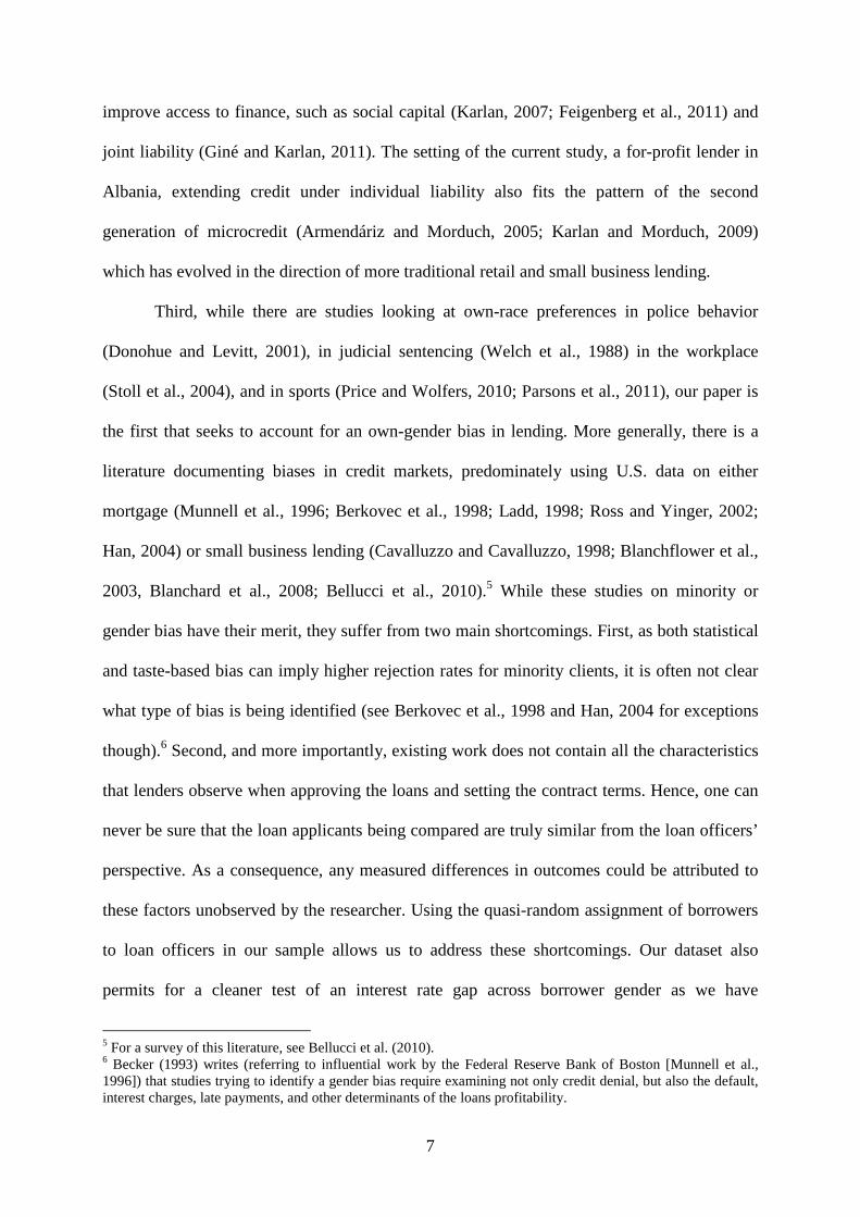
differences in interest rate setting and propensity to monitor.) Figure 1 plots the coefficient
estimate for the female borrower dummy for each loan officer, with the bars representing the
95% confidence interval around the estimates. We find that the median interest rate
differential for female (as opposed to male) borrowers is 21 basis points in the case of male
loan officers and minus 18 basis points in the case of female loan officers.24 While many of
the coefficients are imprecisely estimated, quite a few yield point estimates that are
statistically significantly different from zero. The figure suggests that the bias against the
other gender is prevalent for loan officers of both genders. That is, the majority of male loan
officers have a greater propensity to charge higher interest rates when lending to female
borrowers than the majority of female loan officers. We also note, however, that the
distribution of the own-gender bias is more dispersed in the case of female loan officers, with
the highest three point estimates on the female borrower dummy actually coming from female
loan officers.
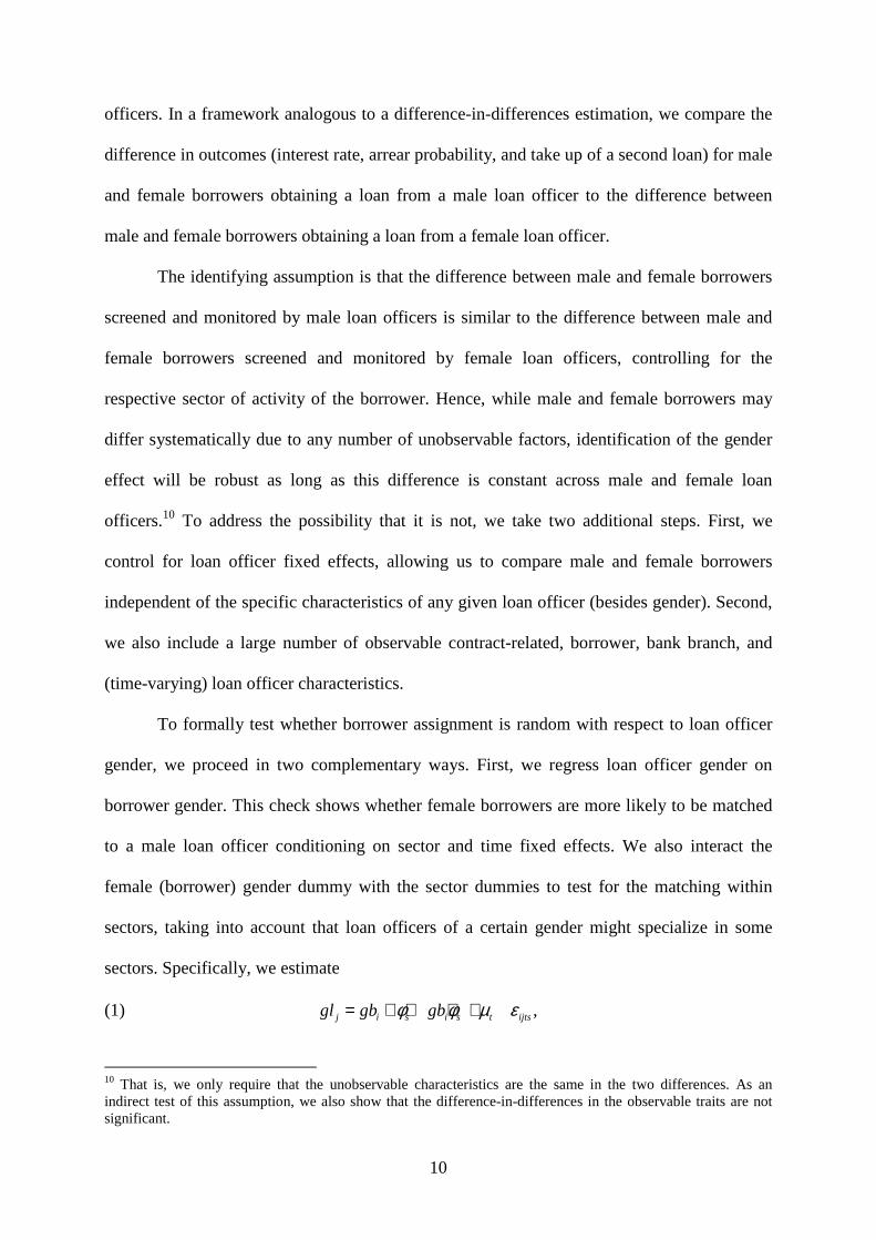
Figure 2 shows a qualitatively similar effect of the own-gender bias from both male
and female loan officers on borrowers’ take-up rates. Here we regress the probability of
returning for a second loan on a female borrower dummy for each loan officer with at least 45
observations, including the same controls as listed above in connection to Figure 1. The
23 Our analysis is similar in spirit to Price and Wolfers (2010). 24 Note that these economic effects differ from the ones reported in Table 4, as we are working with a smaller sample and look at an un-weighted moment.

27
median coefficient estimate of the female borrower dummy is -4.8 percent for male loan
officers and 3.9 percent for female loan officers, thus of similar economic magnitude. The
interpretation is again that there is pro-male bias among male loan officers and a pro-female
bias among female loan officers leading borrowers of the opposite sex to exit at a greater
degree. As before, the dispersion of the coefficient estimates is larger for female than for male
loan officers.
5 Conclusion
Our results suggest that own-gender preferences affect credit market outcomes. In particular,
using a rich loan-level dataset from an Albanian microcredit lender, this paper has three main
findings. First, we identify an own-gender bias in the setting of interest rates. Specifically,
borrowers matched with a loan officer of the other gender pay, on average, 26 to 28 basis
points higher interest rates than if matched with a loan officer of the same sex. Second, the
bias is taste based rather than statistical, as there is no ex-post difference in riskiness across
borrowers matched to a loan officer of the same or the opposite gender. Third, the own-
gender bias has negative repercussions for take up of further loans. Borrowers matched to
loan officers of the opposite sex are between 6.1 and 6.7 percentage points less likely to return
for another loan from the same lender.
We also investigate the sources of the taste-based own-gender bias. We argue and
show that the bias is more pronounced when the social distance between the loan officer in
charge of the loan and the borrower is larger. In addition, the bias increases when loan
officers have more discretion (as measured by financial market competition) in setting interest
rates, that is, applying the bias. Finally, we provide suggestive evidence that the bias stems
from both male loan officers taking action against female borrowers and from female loan
officers acting against male borrowers.

28
Understanding in-group identity, in the form of own-gender preferences, has at least
two implications for the functioning of the credit market. First, identity may affect the
organizational design of financial institutions. Specifically, matching loan officers to
borrowers of the same gender can have repercussions by reducing taste-based biases.
Similarly, the pairing of loan officers and borrowers according to proxies such as age may
also help eliminate existing biases. Second, from a policy perspective, our findings point to
the possibility that financial market competition can be a powerful tool in dampening the
biases of loan officers, and, ultimately, banks, against borrowers of a certain gender.

29
References
Agarwal, S., Wang, F.H., 2009, Perverse Incentives at the Banks? Evidence from a Natural
Experiment, Working Paper, Federal Reserve Bank of Chicago.
Akerlof, G.A., Kranton, R. E., 2000, Economics and Identity, Quarterly Journal of Economics
115(3), 715-753.
Armendariz de Aghion, B., Morduch, J., 2005, The Economics of Microfinance, MIT Press.
Arrow, K. J. 1973. The Theory of Discrimination. In Orley Ashenfelter and Albert Rees, eds.
Discrimination in Labor Markets. Princeton, N.J.: Princeton University Press, 1973. 3-33.
Beck, T., Behr, P., Güttler, A., 2011, Gender and Banking: Are Women better Loan Officers?,
Working Paper.
Becker, G., 1957. The Economics of Discrimination. The University of Chicago Press,
Chicago.
Becker, G., 1993, The Evidence Against Banks Doesn’t Prove Bias, Business Week.
Bellucci, A., Borisov, A.V., Zazzaro, A., 2010, Does Gender Matter in Bank-Firm
Relationships? Evidence from Small Business Lending, Journal of Banking and Finance 34,
2968-2984.
Benjamin, D.J., Choi, J.J., Strickland, A. J., 2010, Social Identity and Preferences, American
Economic Review 100(4), 1913-1928.
Berkovec, J., Canner, G., Gabriel, S., and Hannan T., 1998, Discrimination, competition, and
loan performance in FHA mortgage lending, Review of Economics and Statistics, 80, 241-
250.
Black, S.E., Strahan, P., 2001, The Division of Spoils: Rent Sharing and Discrimination in a
Regulated Industry, American Economic Review 91(4), 814-831.
Blair, I. 2002. The malleability of automatic stereotypes and prejudice. Personality and Social
Psychology Review 6, 242-61.
Blanchard, L., Zhao, B., Yinger, J., 2008, Do lenders discriminate against minority and
woman entrepreneurs?, Journal of Urban Economics, 63(2), 467-497.

30
Blanchflower, D.G., Levine, P.B., Zimmerman, D.J., 2003, Discrimination in the Small
Business Credit Market, Review of Economics and Statistics 85(4), 930-943.
Cavalluzzo, K. S and L. Cavalluzzo, L. C, 1998. Market Structure and Discrimination: The
Case of Small Businesses, Journal of Money, Credit and Banking 30, 771-92.
Chen, Y., Li, S.X., 2009, Group Identity and Social Preferences, American Economic Review
99(1), 431-457
Donohue, J. and S. Levitt, 2001. The impact of race on policing and arrests, Journal of Law &
Economics 44, 367-9.
Drexler, A. and Schoar, A., 2011, Does Soft Information Matter? Evidence From Loan
Officer Absenteeism, Working Paper, MIT.
Feigenberg, B., Field, E., Pande, R., 2011, The Economic Returns to Social Interaction:
Experimental Evidence from Microfinance, Working Paper, Harvard.
Giné, X., and Karlan, D., 2011, Group versus Individual Liability: Short and Long Term
Evidence from Philippine Microcredit Lending Groups, Working Paper, Yale.
Goodwin, S., A. Gubin, S. Fiske, and V. Yzerbyt. 2000. Power can bias impression processes:
stereotyping subordinates by default and by design. Group Processes & Intergroup relations 3,
227-256.
Han, S. 2004. Discrimination in lending: theory and evidence, The Journal of Real Estate
Finance and Economics 29, 5-46.
Hertzberg, A., Liberti, J.M., Paravisini, D., 2010, Information and Incentives Inside the Firm:
Evidence from Loan Officer Rotation, Journal of Finance 65, 795-828.
Karlan D., 2007, Social Connections and Group Banking. Economic Journal 117, F52-F84.
Karlan, D. and J. Morduch. 2009. Access to finance. In: Handbook of Development
Economics 5. Elsevier.
Karlan D. and J. Zinman. 2008. Credit elasticities in less-developed economies: implications
for microfinance. American Economic Review 98, 1040-68.

31
Karlan D. and J. Zinman. 2009. Observing unobservables: identifying information
asymmetries with a consumer credit field experiment. Econometrica 77, 1963-2008.
Ladd, H. 1998. Evidence on discrimination in mortgage lending. Journal of Economic
Perspectives 12, 41-62.
Levine, R., Levkov A., and Rubinstein Y., 2010, Racial Discrimination and Competition,
Working Paper, Brown University.
Munnell, A.H., G.M.B. Tootell, L.E. Browne, J. McEneaney. 1996. Mortgage lending in
Boston: interpreting HMDA data, American Economic Review, 86, 25–53.
Parsons, C.A., Sulaeman, J., Yates, M.C., Hamermesh, D.S., 2011, Strike Three:
Discrimination, Incentives, and Evaluation, American Economic Review 101 (3), 1410-1435.
Phelps, E. 1972. The statistical theory of racism and sexism. American Economic Review 62,
659-61.
Price, J. and J. Wolfers, 2010, Racial discrimination among NBA referees. Quarterly Journal
of Economics 125, 1859-87.
Ross, S.L. and J. Yinger. 2002. The Color of Credit: Mortgage Lending Discrimination,
Research Methodology and Fair-Lending Enforcement. Cambridge, MA: MIT Press.
Statistical Institute of Albania, 2007, Women and Men in Albania 2006, downloadable at
www.instat.gov.al.
Stoll, M. A., S. Raphael, and H. J. Holzer. 2004. "Black Job Applicants and the Hiring
Officer's Race." Industrial and Labor Relations Review, 57, 267-287.
Welch, S., M. Combs and J. Gruhl. 1988. Do black judges make a difference? American
Journal of Political Science 32, 125-36.

32

33

34
Table 1: Test of random assignment (1) (2) (3) (4) Borrower gender -0.1103*** -0.0877*** -0.0306 0.0011 (0.0364) (0.0275) (0.0188) (0.0492) Time FE No Yes Yes Yes Sector FE No No Yes Yes Sector-by-borrower-gender FE No No No Yes Observations 7,891 7,891 7,891 7,891 In this table we regress the loan officer gender on the borrower gender. The dependent variable is a dummy variable that takes on value one if the loan officer is male. The main dependent variable is a dummy variable that takes on value one if the borrower is female. In column (1) we do not include any further control variable. The column (2) regression adds time fixed effects, the column (3) regression further adds sector fixed effects, and the column (4) regressions adds sector-by-borrower-gender fixed effects. Standard errors that are clustered at the branch-sector-year level are shown in parentheses. ***, **, * indicate significance at the 1, 5, and 10 percent level, respectively.

35
Table 2: Test for differences in borrower characteristics Male loan officers Female loan officers Male borrowers Female borrowers t-statistic Male borrowers Female borrowers t-statistic t-statistic Variable (1) (2) (3) = (1) - (2) (4) (5) (6) = (4) - (5) (7) = (3) - (6) Age applicant 41,30 41,99 0,34 40,88 41,46 1,50 0,81
Wage earner 0,46 0,76 2.74** 0,75 0,91 0,40 1,60
Civil status 0,91 0,77 -3.33*** 0,89 0,73 -2.06** 1.92*
Phone availability 0,95 0,92 0,19 0,93 0,91 0,72 -0,32
Applied amount 2.990 2.675 -1,03 3.193 2.769 0,03 -0,80
Applied maturity 585 580 -1,54 625 613 -0,01 0,04
Total assets 26.516 27.577 -1,48 28.204 25.688 -0,65 1,10
Leverage 0,02 0,02 2.20** 0,02 0,02 -1.81* -0,18
Personal guarantee 0,11 0,16 0,69 0,19 0,18 -0,09 0,40
Mortgage guarantee 0,08 0,10 2.25** 0,15 0,13 -0,44 0,03
Chattel guarantee 0,98 0,96 -1,62 0,95 0,94 -0,22 0,47
Working capital 0,10 0,08 0,76 0,08 0,03 -0,98 1,26
Fixed assets 0,48 0,27 -2.59** 0,27 0,12 -0,19 -1,14
Mixed 0,15 0,10 1,26 0,03 0,02 1,12 -0,22
Housing improvement 0,16 0,29 0,36 0,38 0,46 -1,40 0,08
Consumption 0,11 0,26 2.05* 0,24 0,35 1,28 0,54
Others 0,00 0,00 n.a. 0,00 0,00 -1,02 -1,06
Observations 3,057 464 3,521 3,524 846 4,370 7,891 This table contains a test of difference in observable borrower characteristics using a difference-in-difference approach. Columns (1) and (2) show raw means for a set of borrower characteristics of male and female borrowers that are matched with male loan officers. Column (3) shows the t-statistic of a test of difference of the respective borrower characteristic between male and female borrowers with male loan officers. Columns (4) and (5) show raw means of male and female borrowers that are matched with female loan officers. Column (6) shows the t-statistic of a test of difference of the respective borrower characteristic between male and female borrowers with female loan officers. Column (7) shows the t-statistic of a test of differences-in-differences for the respective borrower characteristic. The t-statistics in columns (3) and (6) are estimated conditioned on time, sector, and sector-borrower fixed effects. The t-statistics in column (7) are estimated additionally conditioning on sector-loan officer fixed effects. Standard errors are clustered at the branch-sector-year level. ***, **, * indicate significance at the 1, 5, and 10 percent level, respectively.

36
Table 3: Descriptive statistics (1) (2) (3) (4) (5) (6) (7)
Variable Mean SD Median Male borrower Female borrower Male LO Female LO
Interest rate 0.14 0.02 0.14 0.14 0.14 0.14 0.14 Arrears 0.05 0.23 0.00 0.06 0.04 0.06 0.05 Female 0.17 0.37 0.00 n.a. n.a. 0.13 0.19 Civil status 0.87 0.33 1.00 0.90 0.75 0.89 0.86 Age applicant 41.17 10.29 41.13 41.07 41.65 41.39 40.99 Wage earner 0.65 0.48 1.00 0.61 0.86 0.50 0.78 Total assets 27,244 82,355 16,367 27,420 26,359 26,656 27,718 Leverage 0.02 0.07 0.00 0.02 0.02 0.02 0.02 Applied amount 3,038 2,955 2,086 3,099 2,736 2,948 3,111 Approved amount 2,727 2,861 1,961 2,780 2,458 2,641 2,796 Approved maturity 563 288 540 564 559 542 581 Phone availability 0.94 0.25 1.00 0.94 0.92 0.94 0.93 Personal guarantee 0.16 0.36 0.00 0.16 0.17 0.12 0.19 Mortgage guarantee 0.11 0.32 0.00 0.11 0.12 0.08 0.14 Chattel guarantee 0.96 0.19 1.00 0.97 0.95 0.98 0.95 Destination working capital 0.08 0.28 0.00 0.09 0.05 0.10 0.07 Destination fixed assets 0.33 0.47 0.00 0.37 0.17 0.45 0.24 Destination mixed 0.08 0.27 0.00 0.08 0.05 0.14 0.03 Destination housing improvement 0.30 0.46 0.00 0.28 0.40 0.18 0.40 Destination consumption 0.20 0.40 0.00 0.18 0.32 0.13 0.26 Destination others 0.00 0.02 0.00 0.00 0.00 0.00 0.00 Production 0.18 0.38 0.00 0.20 0.07 0.31 0.07 Transport 0.15 0.36 0.00 0.17 0.05 0.17 0.13 Construction 0.67 0.47 1.00 0.63 0.88 0.52 0.80 Female LO 0.55 0.50 1.00 0.54 0.65 n.a. n.a. Age LO 25.54 4.53 23.89 25.62 25.13 26.74 24.58 Applications per LO 165.49 159.16 121.00 165.64 164.76 159.94 169.97 This table shows descriptive statistics (mean, standard deviation (SD), median) for the main dependent variables interest rate and arrears and the main control variables used in the regression analyses. The columns (1)-(3) show the values for the entire sample, columns (4) and (5) the means for male and female borrowers, and columns (6) and (7) the means for male and female loan officers.

37
Table 4: Own-gender bias and interest rates (1) (2) (3) (4) (5) Panel A: Interest rate Gender*Gender 0.0026** 0.0026** 0.0028** 0.0028** 0.0028**
(0.0011) (0.0011) (0.0011) (0.0011) (0.0011)
Adjusted R-squared 0,4407 0,4435 0,5306 0,5313 0,5395
Observations 7.891 7.885 7.885 7.885 7.885 Panel B: Arrears Gender*Gender 0,0080 0,0105 0,0106 0,0105 0,0106
(0.0137) (0.0148) (0.0146) (0.0146) (0.0147)
Adjusted R-squared 0,0718 0,0764 0,0826 0,0836 0,0834
Observations 7.891 7.885 7.885 7.885 7.885 Loan officer fixed effects Yes Yes Yes Yes Yes Loan officer-specific variables No Yes Yes Yes Yes Borrower-specific variables No No Yes Yes Yes Branch fixed effects No No No Yes Yes Loan characteristics No No No No Yes This table shows regression results with interest rate (Panel A) and arrear occurrence (Panel B) as dependent variables. The table only shows the coefficient for the gender-gender interaction, all further control variables are as indicated in the table, but omitted to save space. Each regression also includes time, sector, sector-borrower, and sector-loan officer fixed effects. Standard errors that are clustered at the branch-sector-year level are shown in parentheses. ***, **, * indicate significance at the 1, 5, and 10 percent level, respectively.

38
Table 5: Own-gender bias and take up of a second loan (1) (2) (3) (4) (5)
Gender*Gender -0.0608** -0.0631** -0.0658** -0.0639** -0.0664**
(0.0304) (0.0309) (0.0282) (0.0300) (0.0279)
Adjusted R-squared 0,0929 0,1944 0,1943 0,2129 0,1833 Observations 5.451 5.445 5.445 2.184 3.261
Loan officer fixed effects Yes Yes Yes Yes Yes Loan officer-specific variables No Yes Yes Yes Yes Borrower-specific variables No No Yes Yes Yes Branch fixed effects No No No Yes Yes Loan characteristics No No No No Yes This table shows regression results with loan take-up as dependent variable. Loan take-up is a dummy variable that takes on value one if borrowers returned to the bank for an additional loan application in case they had been granted a first loan. For this test, the sample period ends on December 31, 2006, less the mean maturity, which is 563 days for all approved loans in the baseline sample. Each regression also includes time, sector, sector-borrower gender, and sector-loan officer fixed effects. Standard errors that are clustered at the branch-sector-year level are shown in parentheses. ***, **, * indicate significance at the 1, 5, and 10 percent level, respectively.

39
Table 6: Heterogeneous effects for take up Small Large No personal Personal Small Big branches branches guarantee guarantee loans loans Gender*Gender -0.2230*** -0,0136 -0.0925*** 0,0481 -0.1115*** -0,0011 (0.0659) (0.0329) (0.0289) (0.0761) (0.0363) (0.0490) P-value of Wald test 0,0026 0,0375 0,0262 Adjusted R-squared 0,2129 0,1833 0,1831 0,2199 0,1760 0,2097 Observations 2.184 3.261 4.202 1.243 2.725 2.720 This table shows regression results with loan take-up as dependent variable. Loan take-up is a dummy variable that takes on the value of one if borrowers returned to the bank for an additional loan application in case they had been granted a first loan. For this test, the sample period ends on December 31, 2006, less the mean maturity, which is 563 days for all approved loans in the baseline sample. All regressions include the control variables that are included in column (4) of Table 4, the results for these are omitted to save space. In columns (1) and (2), we split the sample according to the median number of loan officers by branch and year (12 loan officers). In columns (3) and (4), the sample is split according to whether the borrower had a personal guarantee or not. In columns (5) and (6), the sample is split according to the median loan size (2,191 USD). Standard errors that are clustered at the branch-sector-year level are shown in parentheses. ***, **, * indicate significance at the 1, 5, and 10 percent level, respectively.

40
Table 7: Own-gender bias and social distance Young Old Young Old Low High borrowers borrowers loan officers loan officers experience experience Panel A: Interest rate Gender*Gender 0,0007 0.0041** 0.0052*** 0,0006 0,0031 0.0033**
(0.0013) (0.0016) (0.0018) (0.0015) (0.0024) (0.0015)
P-value of Wald test 0,0949 0,0308 0,9567
Adjusted R-squared 0,5369 0,5335 0,5146 0,5706 0,5514 0,6162
Observations 3.940 3.945 4.045 3.840 4.153 3.732
Panel B: Arrears
Gender*Gender 0,0080 0,0226 0,0001 0,0224 0,0230 -0,0095
(0.0296) (0.0157) (0.0202) (0.0177) (0.0164) (0.0179)
P-value of Wald test 0,6467 0,3447 0,1298
Adjusted R-squared 0,0742 0,0944 0,0716 0,0898 0,0900 0,0766
Observations 3.940 3.945 4.045 3.840 4.153 3.732 This table shows regression results with interest rate (Panel A) and arrear occurrence (Panel B) as dependent variables. All regressions include the control variables that are included in column (4) of Table 4, the results for these are omitted to save space. In columns (1) and (2), the sample is split according to the median borrower age (41 years). In columns (3) and (4), the sample is split according to the median loan officer age (24 years). In columns (5) and (6), the sample is split according to the median loan officer experience measured as the number of loan applications handled by the respective loan officer (121 loan applications handled). Each regression also includes time, sector, sector-borrower, and sector-loan officer fixed effects. Standard errors that are clustered at the branch-sector-year level are shown in parentheses. ***, **, * indicate significance at the 1, 5, and 10 percent level, respectively.

41
Table 8: Own-gender bias and competition Competition Young loan officers Small branches Low High Low competition High competition Low competition High competition Panel A: Interest rate Gender*Gender 0.0039*** 0.0032** 0.0080*** 0,0008 0.0100*** 0,0030
(0.0013) (0.0016) (0.0025) (0.0025) (0.0024) (0.0023)
P-value of Wald test 0,7136 0,0307 0,0225
Adjusted R-squared 0,4278 0,5489 0,4477 0,5269 0,3648 0,5687
Observations 3.557 2.147 1.846 1.010 1.533 1.129
Panel B: Arrears
Gender*Gender -0,0006 0,0412 -0,0035 0,0485 -0,0014 0,0365
(0.0208) (0.0412) (0.0273) (0.1043) (0.0297) (0.0455)
P-value of Wald test 0,3376 0,6007 0,4498
Adjusted R-squared 0,0872 0,0887 0,0595 0,1050 0,0952 0,0379
Observations 3.557 2.147 1.846 1.010 1.533 1.129 This table shows regression results with interest rate (Panel A) and arrear occurrence (Panel B) as dependent variables. All regressions include the control variables that are included in column (4) of Table 4, the results for these are omitted to save space. Further, branch and sector trends are included where possible. In columns (1) and (2), the sample is split according to the median competition measured as the ratio of branches over population in a specific region and year for the time period 2004-2006. Columns (3) and (4) show regression results for below median age loan officers and for low and high competition. Columns (5) and (6) show regression results for below median size branches and for low and high competition. Each regression also includes time, sector, sector-borrower, and sector-loan officer fixed effects. Standard errors that are clustered at the branch-sector-year level are shown in parentheses. ***, **, * indicate significance at the 1, 5, and 10 percent level respectively.

42
Appendix Table A1: Own-gender bias and loan size, repayment burden, and maturity Loan size Repayment burden
(interest rate*loan size)
Maturity
Gender*Gender -46,640 -1,739 -0,2994 (94.220) (9.820) (10.585) Adjusted R-squared 0,6489 0,6418 0,7059 Observations 7.885 7.885 7.885 This table shows regression results with the loan size, repayment burden, and maturity as dependent variables. All regressions include the control variables that are included in column (4) of Table 4, the results for these are omitted to save space. Standard errors that are clustered at the branch-sector-year level are shown in parentheses. ***, **, * indicate significance at the 1, 5, and 10 percent level, respectively.