sgi-v500

STATENS GEOTEKNISKA INSTITUTSWEDISH GEOTECHNICAL INSTITUTE

Varia

500

PÄR-ERIK BACK

Sampling Strategies and Data WorthAnalysis for Contaminated Land� A literature review

LINKÖPING 2001

Varia

Beställning

ISSNISRN

Projektnummer SGIDnr SGI

Statens geotekniska institut (SGI)581 93 Linköping

SGILitteraturtjänstenTel: 013�20 18 04Fax: 013�20 19 09E-post: [email protected]: www.swedgeo.se

1100-6692SGI-VARIA--01/500--SE

100681-9912-718

Swedish Geotechnical institute, SGIChalmers university of technology, CTH

SGI Varia 500

6DPSOLQJ�VWUDWHJLHV�DQG�GDWD�ZRUWKDQDO\VLV�IRU�FRQWDPLQDWHG�ODQG

A literature review

Pär-Erik Back

6*, 2001-01-10 Varia 500 2 (96)

)25(:25'

Contaminated land and groundwater is a problem of growing concern in our society. An in-creased environmental awareness, addressed in Sweden’s new environmental legislation(0LOM|EDONHQ, 1999-01-01), has resulted in land and water contamination now being a majorfactor in land use planning and management, real estate assessment, and property selling. In-vestigation and remediation of contaminated areas are often associated with high costs. TheSwedish EPA currently estimates that there are 22 000 contaminated sites in Sweden, ofwhich approximately 4000 are in need for remediation.

The high costs and large number of contaminated sites are strong incentives for cost-efficientinvestigation and remediation strategies. 0LOM|EDONHQ states that the environmental value ofthe remediation process must be higher than the investment costs. Critical issues to be ad-dressed in order to meet the intentions of 0LOM|EDONHQ and to provide cost-efficient handlingof contaminated sites to landowners, operators, and the society are:

• What level of certainty is required to make sound decisions at a specific site, i.e. where,how and to what extent should sampling be performed?

• What remediation strategy is the most favorable with respect to investment costs and effi-ciency to meet specific clean-up goals?

Risk-based decision analysis is a theoretical approach to handle benefits, investment costs,and risk costs in a structured way to identify cost-efficient alternatives. Today, decisions re-garding investigation strategies and remediation alternatives are in Sweden most often takenwithout completely or openly evaluating the cost-efficiency of alternatives.

The present report is one of two literature reviews prepared within the project 5LVN�EDVHG�GH�FLVLRQ�DQDO\VLV�IRU�LQYHVWLJDWLRQV�DQG�UHPHGLDO�DFWLRQV�RI�FRQWDPLQDWHG�ODQG��5LVNEDVHUDGEHVOXWVDQDO\V�I|U�XQGHUV|NQLQJDU�RFK�nWJlUGHU�YLG�PDUN��RFK�JUXQGYDWWHQI|URUHQDGH�RP�UnGHQ��The project is sponsored by the Swedish Geotechnical Institute (SGI) and carried outin co-operation between SGI and the Department of Geology at Chalmers University. Themain purpose of the project is to evaluate and describe risk-based methods for cost-effectiveinvestigation and remediation strategies with respect to Swedish conditions.�The two reportsare:

• 6DPSOLQJ�VWUDWHJLHV�DQG�GDWD�ZRUWK�DQDO\VLV�IRU�FRQWDPLQDWHG�ODQG, by Pär-Erik Back(Department of Geology, Publ. B 486 and SGI, report Varia 500).

• 'HFLVLRQ�DQDO\VLV�XQGHU�XQFHUWDLQW\, by Jenny Norrman (Department of Geology, Publ. B485 and SGI, report Varia 501).

The main purpose of the reports is to provide comprehensive descriptions of the state of theart of decision analysis and sampling strategies for contaminated land. The reports form animportant basis for future work, not only in the specific project, but also in the wide topic ofrisk-based decision analysis.

Göteborg 2000-12-20

Lars Rosén, Ph.DSupervisor

6*, 2001-01-10 Varia 500 3 (96)

$%675$&7

A literature review of sampling strategies for contaminated soil and groundwater is presented.The different types of uncertainties associated with a site-investigation are reviewed. The un-certainties are classified as pre-sampling, sampling, and post-sampling uncertainties. Theoriesto quantify different types of uncertainties are reviewed, especially the different samplinguncertainties. The particulate sampling theory was found to be of interest because it identifiesall the relevant sampling uncertainties and presents them in a structured way. The question onhow many samples to collect under different conditions is addressed. A conclusion is that thesampling objective must be clearly stated prior to the development of any sampling plan. Twoof the most common sampling objectives are to detect hot spots and to estimate mean con-centrations.

Methods to determine the economic worth of sampling are reviewed. Traditionally, samplinghas been performed with the objective to either (1) minimize uncertainty for a fixed samplingbudget, or to (2) reach a prespecified accuracy at lowest possible cost. However, in recentyears data worth analysis has been used increasingly. The valuable feature of data worthanalysis is the ability to assess the worth of a proposed site-investigation program prior toperforming any sampling or measurements. Data worth analysis is performed in a risk-baseddecision framework by combining decision theory with e.g. geological, geochemical, hydro-geological, and economic information. A conclusion is that the use of data worth analysis forcontaminated land problems has a potential but the complexity of existing methods has lim-ited its use. To be used on a more regular basis, data worth methods need to be further devel-oped.

A review of more than 30 related software packages is presented in an appendix. It was foundthat public domain or low cost commercial software packages exist for a number applicationsrelated to site-investigations, e.g. sampling design, data evaluation, geostatistical techniques,stochastic simulation, data worth analysis, and decision analysis.

.H\ZRUGV� sampling, uncertainty, risk, data worth, contamination, soil, groundwater

&217(176

)25(:25'

$%675$&7

� ,1752'8&7,21��

1.1 BACKGROUND................................................................................................................................ 61.2 THE PROBLEM: DECISION UNDER UNCERTAINTY............................................................................ 71.3 PURPOSE ........................................................................................................................................ 81.4 LIMITATIONS.................................................................................................................................. 8

� 81&(57$,17<�,1�*(1(5$/��

2.1 QUANTITIES, PARAMETERS, CONSTANTS AND VARIABLES.............................................................. 92.2 ERROR VS. UNCERTAINTY, PROBABILITY AND RISK...................................................................... 102.3 TYPES AND SOURCES OF UNCERTAINTY........................................................................................ 102.4 QUANTIFICATION OF UNCERTAINTY ............................................................................................. 14�� &ODVVLFDO�VWDWLVWLFV�� %D\HVLDQ�VWDWLVWLFV �� 6SDWLDO�VWDWLVWLFV ��

2.5 MODELLING UNCERTAINTY.......................................................................................................... 20�� 7KH�GHWHUPLQLVWLF�DSSURDFK �� 7KH�SUREDELOLVWLF�DSSURDFK�� 7KH�SRVVLELOLW\�DSSURDFK��

� 35(�6$03/,1*�81&(57$,17< ��

3.1 INTRODUCTION............................................................................................................................. 223.2 UNCERTAINTY IN Á-PRIORI KNOWLEDGE...................................................................................... 223.3 UNCERTAINTY IN CONCEPTUAL MODELS...................................................................................... 223.4 COMBINING HARD AND SOFT INFORMATION................................................................................. 243.5 UNCERTAINTY IN QUANTITATIVE MODELS ................................................................................... 26

� 6$03/,1*�81&(57$,17<��

4.1 INTRODUCTION............................................................................................................................. 284.2 SAMPLING KEY TERMS ................................................................................................................. 284.3 SAMPLING OBJECTIVES................................................................................................................. 294.4 PLANNING PHASE (DQOS AND QA/QC)....................................................................................... 304.5 SAMPLING PATTERN DESIGN......................................................................................................... 314.6 SAMPLING THEORIES.................................................................................................................... 354.7 PARTICULATE SAMPLING THEORY................................................................................................ 35�� ,QWURGXFWLRQ �� 6DPSOLQJ�HUURUV �� +HWHURJHQHLW\�� 5HSUHVHQWDWLYHQHVV �� 6DPSOH�6XSSRUW �� 'LPHQVLRQ�RI�ORWV �� $SSOLFDWLRQ�WR�HQYLURQPHQWDO�SUREOHPV ��

4.8 COMPOSITE SAMPLING................................................................................................................. 434.9 MEAN CONCENTRATION – CLASSICAL APPROACHES..................................................................... 44�� 5DQGRP�VDPSOLQJ�XQFHUWDLQW\ �� 6\VWHPDWLF�VDPSOLQJ�XQFHUWDLQW\�� *HRFKHPLFDO�YDULDELOLW\��SRSXODWLRQ�YDULDELOLW\�� 0RGHOV�RI�WRWDO�UDQGRP�XQFHUWDLQW\�� 0RGHOV�RI�WRWDO�V\VWHPDWLF�XQFHUWDLQW\�� 5HTXLUHG�QXPEHU�RI�VDPSOHV��

4.10 DETECTION OF HOT SPOTS ....................................................................................................... 524.11 DELINEATION OF CONTAMINATED AREAS................................................................................ 54

6*, 2001-01-10 Varia 500 5 (96)

� 3267�6$03/,1*�81&(57$,17<��

5.1 ERRONEOUS SAMPLES .................................................................................................................. 555.2 UNCERTAINTY IN LABORATORY ANALYSES PLANS....................................................................... 555.3 FIELD AND LABORATORY ANALYSES............................................................................................ 565.4 DATA EVALUATION ...................................................................................................................... 57

� '$7$�:257+�$1$/<6,6�$1'�&267�())(&7,9(1(66��

6.1 INTRODUCTION............................................................................................................................. 596.2 DECISION THEORY........................................................................................................................ 596.3 TOOLS FOR DATA WORTH ANALYSIS............................................................................................. 60�� 3D\RII�WDEOHV �� 'HFLVLRQ�WUHHV�DQG�HYHQW�WUHHV�� ,QIOXHQFH�GLDJUDPV�� ([SHUW�V\VWHPV��

6.4 STRATEGIES FOR DATA WORTH ANALYSIS.................................................................................... 62�� 7UDGLWLRQDO�DSSURDFK��)L[HG�FRVW�RU�IL[HG�XQFHUWDLQW\ �� 0LVFODVVLILFDWLRQ�FRVW�DQG�ORVV�IXQFWLRQV �� 8QFHUWDLQW\�EDVHG�VWRSSLQJ�UXOHV �� %D\HVLDQ�GHFLVLRQ�DQDO\VLV�� 2SWLPLVDWLRQ�DSSURDFKHV �� 5XOH�EDVHG�DGDSWLYH�VDPSOLQJ �� 6DPSOLQJ�IRU�PRGHO�GLVFULPLQDWLRQ��

� ',6&866,21 ��

7.1 GENERAL............................................................................................................................... ....... 757.2 PRIOR INFORMATION AND EXPERT KNOWLEDGE........................................................................... 757.3 MODELS ....................................................................................................................................... 757.4 PARTICULATE SAMPLING THEORY ................................................................................................ 757.5 SAMPLING ERRORS ....................................................................................................................... 767.6 SAMPLING STRATEGIES ................................................................................................................ 767.7 DATA WORTH ............................................................................................................................... 76

5()(5(1&(6��

$33(1',;��62)7:$5(�3$&.$*(6

6*, 2001-01-10 Varia 500 6 (96)

�� ,1752'8&7,21

�� %DFNJURXQG

Contaminated soil and groundwater is a problem that has received increased attention inthe last decade. The risk of exposure to contaminants for humans and the environmentmakes it necessary to investigate the degree of contamination at a site. Usually the in-vestigation of a contaminated site results in a risk assessment, where the risk for humansand the environment is assessed. Sometimes, a preliminary assessment of the site is per-formed before any samples or measurements have been taken. This preliminary assess-ment is based on á-priori knowledge about the site, such as the type of contaminants thathas been used at the site, the geologic conditions, spill events etc.

When a site with contaminated soil or groundwater is investigated, a number of deci-sions have to be made. They are of different nature but typically include which sam-pling strategy to use (how many samples to take, where to take them, which media tosample, control and duplicate samples etc.) and if remediation of the site is necessary.Usually, many of these, and similar questions, have no easy answer, mainly due to un-certainties in the site-investigation.

All stages of a site-investigation involve uncertainties. These include uncertainties in:- á-priori knowledge about the site,- conceptual models of the site,- sampling, handling, field measurements and laboratory analyses,- data handling and prediction of contaminant transport, and- risk assessment

This can be summarised as uncertainties in (1) contaminant characterisation and (2)geological characterisation. The site-investigation results in an estimate of the extent ofthe contamination at the site. The level of contamination is uncertain but will influencethe remediation costs. If there is a large uncertainty in the estimate of contamination, theremediation costs will also be uncertain. Often, the remediation cost will be muchhigher than anticipated. Therefore, it would be preferable if the uncertainties in a site-investigation could be estimated.

Because of stiff competition on the market the consultant with the cheapest site-investigation (smalles number of samples) often gets the job (Bosman, 1993). A conse-quence is that it will be difficult to discriminate between “nothing found” because therewas nothing there or “nothing found” because of a poor site-investigation (Bosman,1993). The latter may well be regarded as a success by the involved parties but may infact lead to long term human health or environmental effects. It is obvious that the un-certainties are large in many site-investigations of contaminated soil and groundwater.Often, the overall uncertainty is underestimated, especially in cases where only a fewfield samples has been collected, and data analysis cannot recover more informationthan the samples contain (Flatman and Yfantis, 1996). Collecting only a few samplescan therefore result in poor site characterisation, which in turn can result in poor andexpensive remediation decisions (James and Gorelick, 1994).

Today, laboratory methodology has reached a point where analytical error contributesonly a very small portion of the total variance seen in data (Mason, 1992; Shefsky,1997). Typically, errors in the taking of field samples are much greater than preparation,

6*, 2001-01-10 Varia 500 7 (96)

handling, analytical, and data analysis errors (van Ee et al., 1990). Unfortunately, manydecisions are made in ignorance or contempt of the uncertainty of the sample data(Taylor, 1996). However, neglecting uncertainties does not mean that they do not exist(Lacasse and Nadim, 1996). Instead, uncertainties need to be considered and if possiblebe reduced.

There are several ways to reduce the overall uncertainty, but the most effective one isoften to increase the number of samples taken, provided that the samples are represen-tative of the sample location. This will usually reduce the uncertainty but increase thecosts of sampling and analyses. Also, in many cases the uncertainty can be economi-cally reduced by going from a random to a spatial variable sampling design (Flatmanand Yfantis, 1996).

�� 7KH�SUREOHP��'HFLVLRQ�XQGHU�XQFHUWDLQW\

The main problems that will be addressed in this report is:

1. how to quantify the uncertainties that exist in a site-investigation, and2. how to find an “optimal” level of uncertainty (i.e. optimal to make the proper deci-

sion), with respect to sampling.

These problems are a part of the main problem at a contaminated site, namely how tomake GHFLVLRQV�XQGHU�XQFHUWDLQW\. Therefore, these questions should be handled in aframework based on GHFLVLRQ�DQDO\VLV. The principle of decision analysis is how tomake well-founded, defensible decisions under uncertainty. Typically, a reduction inuncertainty has a cost, which can be weighed against the benefit of making a more well-founded decision. It is practical to use monetary terms to quantify the costs and benefits,as described in chapter 6, but there are several other methods.

The optimal level of uncertainty in a site-investigation is reached when the cost for ad-ditional information (from additional sampling etc.) is equal to the expected benefitsassociated with the new information. Additional information is only cost-efficient up tothat point. If the cost for additional information exceeds the benefit, sampling is nolonger cost-efficient. 'DWD�ZRUWK�DQDO\VLV is thus the key to a cost-efficient site-investigation. In a decision analysis framework the data worth analysis sets the stoppingrule when no additional collection of information should be made. More informationwill have a cost but the decision will not be sufficiently more well-founded to justifythat cost. Decision analysis can also be used to compare alternative data-collection pro-grammes, such as different sampling strategies.

All relevant uncertainties in the pre-sampling, sampling and post-sampling phases of theinvestigation have to be handled to make the data worth analysis complete. Optimally, itshould be possible to quantify all uncertainties involved. Taking all uncertainties intoconsideration will make it possible to demonstrate the overall uncertainty of a site-investigation, especially the uncertainty associated with the sampling process.

6*, 2001-01-10 Varia 500 8 (96)

�� 3XUSRVH

The purpose of the literature review is to present the state-of-the-art regarding uncer-tainties and data worth analysis in site-investigations. The focus is on sampling and dataworth analysis. Both contaminated soil and groundwater are addressed. The literaturereview covers several related topics, primarily the following:

- Uncertainty in general- Uncertainty in geologic and conceptual models (e.g. geologic interpretation and de-

scription)- Sampling uncertainty and sampling strategies- Data worth analysis

A review of relevant software packages is also presented in an appendix.

�� /LPLWDWLRQV

In the literature review, the focus of uncertainty in site-investigations is on geochemicalproperties, but geologic and hydraulic properties are also considered. The two latter areassociated with the important concepts of SDUDPHWHU�XQFHUWDLQW\ and PRGHO�XQFHUWDLQW\.

Methods to estimate the uncertainty in field and laboratory analyses are only addressedin short. These methods have been described thoroughly in the chemical analysis lit-erature. Also, uncertainty in human health and ecological risk assessments is importantto be aware of but is not addressed in the report. This question is more related to reme-diation decision problems.

In the literature there is an abundance of qualitative routines for sampling but they areof minor concern in this report. The reason is that they rarely support any quantitativeestimation of uncertainty.

6*, 2001-01-10 Varia 500 9 (96)

�� 81&(57$,17<�,1�*(1(5$/

�� 4XDQWLWLHV��SDUDPHWHUV��FRQVWDQWV�DQG�YDULDEOHV

A quantity is something that can be quantified in some way. Parameter is a similar term(note that the term parameter has a more specific definition in statistics). Quantities andparameters can be classified into a number of groups. Morgan and Henrion (1990) dis-tinguish at least 7 different types of quantity:

✓ Empirical quantities✓ Defined constants✓ Decision variables✓ Value parameters✓ Index variables✓ Model domain parameters✓ Outcome criteria

These quantities can be explained in the following way, primarily as described byMorgan and Henrion (1990):

(PSLULFDO�TXDQWLWLHV represent measurable properties of the real world, such as hydrau-lic conductivity. The uncertainty of an empirical quantity can be expressed in the formof a probability density function (PDF). Often, the empirical quantities constitute themajority of quantities in models and they are often uncertain. The commonly used term“parameter uncertainty” refers to uncertainty in empirical quantities.

'HILQHG�FRQVWDQWV are by definition certain, such as the mathematical constant π or thenumber of days in December. Many physical constants, such as the gravitational con-stant, are actually empirical quantities but with only a small degree of uncertainty.

A GHFLVLRQ�YDULDEOH (or control variable) is a quantity for which it is up to the risk ana-lyst or the decision-maker to select a value. Examples of decision variables at a site-investigation are the number of sampling points and the sampling depth. A decisionvariable has no inherent uncertainty but the difficulty is to find its “best” value.

9DOXH�SDUDPHWHUV�represent values or preferences of the decision-maker. Examples ofvalue parameters are the discount rate in cost-benefit analysis, parameters of risk toler-ance or risk aversion, and “value of life”. It is debatable if value parameters can betreated as probabilistic. Usually it is a serious mistake to treat value parameters in thesame way as empirical quantities. However, the difference between a value parameterand an empirical quantity is not always clear. It is also a matter of intent and perspec-tive.

,QGH[�YDULDEOHV�are used to identify a location in the spatial or temporal domain of amodel. Examples include x and y co-ordinates in a 2-dimensional model. Index-variables are certain by definition.

0RGHO�GRPDLQ�SDUDPHWHUV specify the domain of the modelled system, generally byspecifying the range and increments for index variables. Domain parameters define thelevel of detail of a model, both spatially and temporally. Examples of domain parame-ters are grid spacing in a model, time increment in transient simulations etc. Usually,

6*, 2001-01-10 Varia 500 10 (96)

there is uncertainty about the appropriate values for domain parameters but it is inap-propriate and impractical to represent the uncertainty with a probability distribution.The choice of value is up to the modeller.

2XWFRPH�FULWHULD are variables used to measure the desirability of possible outcomes ofa model. Examples include the calculated measure of risk in a risk model. Outcome cri-teria will be deterministic or probabilistic depending on whether any of the input quan-tities on which they depend are probabilistic.

Gorelick et al. (1993) make a distinction between parameters and variables in ground-water problems. They use the term parameter for time-independent properties such ashydraulic conductivity, while the term variable is used for time-dependent indicatorssuch as hydraulic head and contaminant concentration.

�� (UURU�YV��XQFHUWDLQW\��SUREDELOLW\�DQG�ULVN

It is important to notice the difference between terms like error and uncertainty, al-though they often are used as synonyms. Terms like uncertainty, reliability, confidenceand risk are probability-related and refer to á priori conditions, i.e. before an event.Probability is related to a statistical confidence before an event (Myers, 1997). Thus, anestimate is only a rational “guess” of the outcome. Error, on the other hand, can only bemeasured á posteriori, i.e. after an event has occurred. It is not possible to know whatthe errors will be before the event has occurred. Error relates to a known outcome orvalue and is therefore a more concrete item than the probability-related terms (Myers,1997). However, uncertainty may be present even after an event has occurred if the er-ror is not completely known.

As the reader will soon be aware of the distinction between error and uncertainty hasnot been maintained in the rest of this report. The main reason is that the two conceptsoften are used more or less synonymous by many authors. Therefore, the concept cho-sen by the author has been kept. The mixed use of uncertainty and error in practical ap-plications can be explained in the following way: Prior to an investigation it is usuallyknown that activities, such as sampling, will result in some error but the magnitude ofthe error is uncertain. Therefore, trying to estimate the error prior to investigation is away of handling the uncertainty. This explains way the two terms often are used assynonyms.

Risk is often defined as a combination of the probability of a harmful event to occur andthe loss (consequences) of the outcome of this event. However, there are numerousother definitions, which makes it necessary to clearly define the term “risk” in each ap-plication it is used to avoid misinterpretation.

�� 7\SHV�DQG�VRXUFHV�RI�XQFHUWDLQW\

It is not an easy task to define what uncertainty really is. The variety of types andsources of uncertainty, along with the lack of agreed terminology, can generate consid-erable confusion (Morgan and Henrion, 1990). Rowe (1994) defines uncertainty as ab-sence of information, information that may or may not be obtainable. Taylor (1993)defines uncertainty as a measure of the incompleteness of one´s knowledge or informa-

6*, 2001-01-10 Varia 500 11 (96)

tion about a quantity whose true value could be established with a perfect measuringdevice. Though not easily defined, it is important to distinguish between the differenttypes and sources of uncertainty. Morgan and Henrion (1990) argue that probability isan appropriate way to express some of these kinds of uncertainty, but not all of them. Intheir view, the uncertainties should be handled differently depending on what type ofquantity they refer to (see section 2.1).

Rowe (1994) distinguishes four classes of uncertainty:1. Temporal, i.e. uncertainty in future and past states2. Structural, i.e. uncertainty due to complexity3. Metrical, i.e. uncertainty in measurements4. Translational, i.e. uncertainty in explaining uncertain results.

All four classes occur at the same time but for a specific problem one or more domi-nates.

For human health risk assessments Hoffman and Hammonds (1994) refer to the Inter-national Atomic Energy Agency, who distinguishes between Type A and Type B un-certainty. Uncertainty about a deterministic quantity with respect to the assessment endpoint is called Type B uncertainty (example: specific individual). When the assessmentend point is a distribution of actual exposures or risks, the uncertainty is of Type A (ex-ample: a group of individuals). To separate these uncertainties in a model, it is neces-sary to perform stochastic simulation in two dimensions.

Lacasse and Nadim (1996) divide uncertainties associated with geotechnical problemsinto two categories:1. aleatory (inherent or natural) uncertainties, i.e. uncertainty that cannot be reduced2. epistemic (due to lack of knowledge) uncertainties, i.e. uncertainty that can be re-

ducedThis grouping excludes human error, which would fall into a third category.

It is quite common to distinguish between uncertainty in quantity (SDUDPHWHU�XQFHU�WDLQW\) and uncertainty about model structure (PRGHO�XQFHUWDLQW\). Morgan and Henrion(1990) classify uncertainty in empirical quantities (se above) in terms of the sourcesfrom which it can arise:

� Random error and statistical variation (precision)� Systematic error and subjective judgement (bias)� Linguistic imprecision� Variability� Inherent randomness� Disagreement� Approximations

5DQGRP�HUURU�DQG�VWDWLVWLFDO�YDULDWLRQ is the kind of uncertainty that has been studiedthe most. No measurement of an empirical quantity can be absolutely exact; there willalways be some uncertainty. This is especially true in site-investigations of contami-nated land. There are a variety of well-known statistical techniques for quantifying thisuncertainty. Random error can be reduced by taking sufficient number of measurements(Morgan and Henrion, 1990). Random error is often expressed as SUHFLVLRQ (Figure 1).

6*, 2001-01-10 Varia 500 12 (96)

Precision is defined as “>W@KH�FORVHQHVV�RI�DJUHHPHQW�EHWZHHQ�LQGHSHQGHQW�WHVW�UHVXOWVREWDLQHG�XQGHU�VWLSXODWHG�FRQGLWLRQV” (International Organization for Standardization,1994). Another name for random uncertainty is VWRFKDVWLF�XQFHUWDLQW\ (U.S. EPA,1997c).

6\VWHPDWLF�HUURU is defined as the difference between the true value of a quantity and thevalue to which the mean of the measurements converge as more measurements aretaken. It cannot be reduced by more measurements. Systematic error often comes todominate the overall error and it has been found that it is almost always underestimated.This should not be surprising, since systematic errors often are unknown at the time,which calls for subjective estimates of this error. Systematic error is often expressed asELDV (Figure 1). A positive counterpart to bias has been presented by the InternationalOrganization for Standardization (1994) by inventing the term WUXHQHVV. Trueness isdefined as “>W@KH�FORVHQHVV�RI�DJUHHPHQW�EHWZHHQ�WKH�DYHUDJH�YDOXH�REWDLQHG�IURP�DODUJH�VHULHV�RI�WHVW�UHVXOWV�DQG�DQ�DFFHSWHG�UHIHUHQFH�YDOXH”. Another name for system-atic uncertainty is PHWKRGLFDO�XQFHUWDLQW\ (U.S. EPA, 1997c).

Together, random errors and systematic errors constitute the DFFXUDF\ of a measure-ment. Accuracy is a measure of the closeness of a measurement to the true value(Gilbert, 1987), i.e. the absence of error. The International Organization for Standardi-zation (1994) defines accuracy as “>W@KH�FORVHQHVV�RI�DJUHHPHQW�EHWZHHQ�D�WHVW�UHVXOWDQG�WKH�DFFHSWHG�UHIHUHQFH�YDOXH” and includes trueness and precision. The definition ofaccuracy is controversial; several definitions exist and they are not in agreement witheach other (Pitard, 1993). Pitard (1993) argues that it is incorrect to include the notionof precision in the definition of accuracy since accuracy is independent of precision.U.S. EPA has recommended eliminating the use of the term accuracy because of lack ofstandard to determine it (Mason, 1992).

)LJXUH�� 3DWWHUQV�RI�VKRWV�DW�D�WDUJHW��DIWHU�*LOEHUW��D��KLJK�ELDV��ORZ�SUHFLVLRQ� �ORZ�DFFXUDF\�E��ORZ�ELDV��ORZ�SUHFLVLRQ� �ORZ�DFFXUDF\�F��KLJK�ELDV��KLJK�SUHFLVLRQ� �ORZ�DFFXUDF\�G��ORZ�ELDV��KLJK�SUHFLVLRQ� �KLJK�DFFXUDF\

a) b)

c) d)

6*, 2001-01-10 Varia 500 13 (96)

/LQJXLVWLF�LPSUHFLVLRQ is best illustrated by an example. Consider a site where the levelof the groundwater table should be determined. The statement “the groundwater level islow” is an example of linguistic imprecision. In a site-investigation linguistic impreci-sion should be minimised and preferably eliminated.

9DULDELOLW\ is the uncertainty due to a quantity that varies over space or time. One ex-ample is when the groundwater level in a monitoring well varies over time. Anotherexample is when the concentration of a contaminant varies over space at a contaminatedsite. Similar terms are SRSXODWLRQ�YDULDELOLW\, JHRFKHPLFDO�YDULDELOLW\ or HQYLURQPHQWDOYDULDELOLW\. Taking more samples cannot reduce variability but our knowledge of thevariability can be increased (Morgan and Henrion, 1990). Variability relates to randomerror and statistical variation in spatial statistical problems. Often, the real variation ofcontaminant concentration is expressed as a variance.

,QKHUHQW�UDQGRPQHVV is sometimes distinguished from other types of uncertainty. Itcontains randomness that is impossible to reduce by further investigation, in principle orin practice. An example is the inherent randomness in meteorological systems that makeit impossible to correctly make long-range weather predictions (Morgan and Henrion,1990).

'LVDJUHHPHQW is a kind of uncertainty, especially in risk and policy analysis. A typicalexample is the disagreement among experts about a quantity. This type of uncertainty isimportant in situations where a decision must be made before further investigation aboutthe quantity can be carried out. In risk-based decision analysis there may also be dis-agreement about how the failure criterion should be defined (see chapter 6) and aboutacceptable risks.

$SSUR[LPDWLRQ�uncertainty arises because of the simplifications that are unavoidablewhen real-world situations are modelled. In many site-investigations the hydraulic con-ductivity is assumed to be constant in space, which is an approximation. It is often diffi-cult to know how much uncertainty is introduced by a given approximation (Morganand Henrion, 1990).

Usually, XQFHUWDLQW\�DERXW�PRGHO�VWUXFWXUH is more important than uncertainty about thevalue of a parameter. In fact, the distinction between model uncertainty and parameteruncertainty can be rather slippery (Morgan and Henrion, 1990). Model uncertainty isdue to idealisations made in the physical formulation of a problem (Lacasse and Nadim,1996). Model uncertainty is further discussed in section 3.5. Sturk (1998) distinguishesbetween three types of parameter uncertainty; (1) statistical uncertainty, (2) measure-ment errors, and (3) gross errors.

In site-investigations of contaminated land Ramsey and Argyraki (1997) uses the termPHDVXUHPHQW�XQFHUWDLQW\ as a way of characterising uncertainty in site-investigations. Inthis concept field sampling and chemical analysis are just two parts of the same meas-urement process. Measurement uncertainty is the total uncertainty of the whole meas-urement process and it has four potential components:

6*, 2001-01-10 Varia 500 14 (96)

1. Sampling precision (random error)2. Sampling bias (systematic error)3. Analytical precision (random error)4. Analytical bias (systematic error)

Ramsey et al. (1995) applied this view when estimating the uncertainty of the meanconcentration of lead and copper at a site, as described in section 4.9.4. Note that otherauthors may refer to measurement uncertainty as the analytical uncertainty, for exampleTaylor (1996).

Christian et al. (1994) have categorised uncertainty in soil properties according toFigure 2. These uncertainties can be compared to random error, systematic error, andvariability as described above.

Uncertainty in Soil Properties

Data Scatter Systematic Error

Real SpatialVariation

RandomTesting Errors

Statistical Errorin the Mean

Bias in MeasurementProcedures

)LJXUH�� &DWHJRULHV�RI�XQFHUWDLQW\�LQ�VRLO�SURSHUWLHV��DIWHU�&KULVWLDQ�HW�DO��

Sturk (1998) classifies uncertainty in geological engineering problems into threeclasses; (1) inherent variability, (2) modelling uncertainty, and (3) parameter uncer-tainty. Inherent variability arises because the subsurface is composed of different mate-rials. Modelling and parameter uncertainty is described in chapter 3.

�� 4XDQWLILFDWLRQ�RI�XQFHUWDLQW\

�� &ODVVLFDO�VWDWLVWLFV

In classical statistics a frequentistic view is applied. This implies that a probability dis-tribution can only be created by the collection of data. If no data exists there will be noway of quantifying the uncertainty (the uncertainty is infinite), and it will make no sensedefining a probability distribution. As more and more data are collected, the confidencein calculated distribution parameters increases. Two of the most important probabilitydistributions are the 1RUPDO and the /RJQRUPDO distribution.

Many of the tools used in classical statistics assume normally distributed data, whichmakes calculations relatively simple compared to if this assumption is not employed.This can be a problem, since contaminant concentrations in soil are inherently lognor-mally distributed (Ball and Hahn, 1998). The methods of classical statistics will not be

6*, 2001-01-10 Varia 500 15 (96)

discussed further since they can be found in any textbook on the subject. An excellentpresentation of classical statistical methods for environmental sampling problems can befound in Gilbert (1987). U.S. EPA (2000b) describes a large number of statistical meas-ures, plots and statistical tests for environmental sampling.

Thompson and Ramsey (1995) note that uncertainty can be expressed as a standard de-viation (the standard uncertainty) or as a half-range (the expanded uncertainty). Thelatter is obtained by multiplying the standard uncertainty by a coverage factor, normallybetween 2 and 3.

If few data exist it may be problematic to use classical statistics to estimate the uncer-tainty.Lacasse and Nadim (1996) mention that VKRUW�FXW�HVWLPDWHV can be used in these cases.This is a method to estimate the standard deviation for limited data sets of symmetricaldata. Ball and Hahn (1998) also address the issue of small data sets, but for environ-mental problems, and a small literature review on the subject is presented. They con-clude that the issue of small data sets is not addressed directly in current textbooks onstatistics for environmental problems.

Myers (1997) concludes that care should be used when applying classical statisticalmodels to spatial data since classical statistics assumes uncorrelated data while spatialdata often is correlated.

�� %D\HVLDQ�VWDWLVWLFV%D\HV�WKHRUHPThe base for Bayesian statistics is Bayes´ theorem. It is a logical extension of the basicrules of probability. Bayes´ theorem can be formulated as a conditional probability(Alén, 1998; Vose, 1996):

( ) ( )( )

( ) ( )( ) ( )∑

=

⋅

⋅==

Q

L

LL

LLL

L

$3$%3

$3$%3

%3

%$3%$3

1

I

where 3($L%) represents the probability of event $L given that event % has occurred.An advantage of Bayesian statistics compared to classical statistics is that all sources ofinformation can be considered. This includes direct evidence from statistical samplingas well as indirect evidence of whatever kind available from past experience of theanalyst or other experts (Hoffman and Kaplan, 1999).

%D\HVLDQ�XSGDWLQJIn Bayesian statistics Bayes´ theorem is employed to determine SRVWHULRU probabilitydistributions of a variable by combining SULRUL information with observed data (Vose,1996) (a more formally correct term for probability distributions is probability densityfunctions, PDFs). In other words, the prior information is updated with additional data,e.g. from sampling, to reduce the uncertainty. Sometimes an analysis is performed whenprior information is available but before additional information has been collected. Thisstage is called SUHSRVWHULRU analysis (Freeze et al., 1992). To further reduce the uncer-tainty another sampling round can be performed. The posterior estimate now becomes

6*, 2001-01-10 Varia 500 16 (96)

the prior estimate, which can be used together with the new data to produce anotherposterior estimate with less uncertainty. This step can be repeated several times.McLaughlin et al. (1993) calls this procedure “sequential updating”.

As formulated above, Bayes´ theorem is relatively simple but when applied to continu-ously distribution functions the mathematics can become laborious. Therefore, riskanalysts appear to split into two camps: those who use Bayes´ theorem extensively andthose who do not (Vose, 1996).

3ULRU�3')VThere is an important aspect of Bayesian statistics that often is used even if calculationwith Bayes´ theorem is not performed. In contrary to classical statistics it is possible todefine probability density functions (PDFs) although no “hard data” exists. SubjectivePDFs can be used to characterise an individual’s belief about the value of a parameter(Hammitt, 1995). Such SULRU�GLVWULEXWLRQV should reflect the prior knowledge beforemeasurements have been made, something that is not possible in classical statistics.Therefore, the difference between classical and Bayesian statistics is more or less philo-sophical since the mathematics are the same. However, some authors, e.g. Rowe (1994),argue that probability distributions should only be used to address future temporal un-certainty since probability does not exist in the past, and that they are improperly usedotherwise.

Prior distributions are defined at early stages in a project when measurements arescarce. If sufficient KDUG�GDWD is available it is relatively easy to define a probabilitydistribution by classical statistical methods. +DUG�GDWD are direct measurements or ob-servations (Koltermann and Gorelick, 1996). If measurements or similar hard data is notavailable, so called VRIW�GDWD can be used to define a prior distribution. The soft data areindirect information such as historical information, expert opinions, professional experi-ence and all other information that may be difficult to quantify. Freeze et al. (1992) andJohnson (1996) also refer to indirect measurements as soft data, such as geophysicalmeasurements.

A distribution based on soft data is to some extent subjective or judgmental but shouldcontain the uncertainty associated with the information. Judgmental approaches to gen-erate probability distributions can be formal or informal in nature (Taylor, 1993). For-mal methods are to be preferred. Several formal methods to assign subjective probabili-ties and construct subjective probability distributions exist. A review of these methodsis given by Olsson (2000). Vose (1996) also discusses how distributions are definedfrom expert opinion and the sources of error in subjective estimation. Many proceduresfor combining information from multiple sources to construct prior distributions havebeen proposed but none are clearly superior (Hammitt and Shlyakhter, 1999). It is bene-ficial if objective and subjective information can be considered together when distribu-tions are developed (Taylor, 1993).

Examples of probability distributions can be found in many textbooks on probabilitytheory. Typical examples of distributions constructed from soft data are the QRQ�SDUDPHWULF�GLVWULEXWLRQV, which include the Cumulative, Discrete, Histogram, General,Triangular, and Uniform (Rectangular) distributions (Vose, 1996). Common SDUDPHWULFGLVWULEXWLRQV include the Exponential, Normal (Gaussian) and Lognormal distributions.

6*, 2001-01-10 Varia 500 17 (96)

Vose (1996) argues that parametric distributions based on subjective information shouldbe used with caution.

The shape of the prior distribution is very important since it reflects the current infor-mation. However, there is a well-documented tendency of both experts and lay peopleto underestimate uncertainty in their knowledge of quantitative information (Hammitt,1995; Hammitt and Shlyakhter, 1999). This will often result in a prior distribution thatis too narrow (Taylor, 1993). It has been concluded that empirical distributions ofmeasurement and forecast errors have much longer tails than can be described by aNormal distribution (Hammitt and Shlyakhter, 1999). Hammitt (1995) suggests that thetendency for overconfidence most be taken into account when the prior distribution isestimated. Some researchers recommend that the uncertainty should be increased delib-erately to combat this bias (Taylor, 1993).

In Bayesian statistics all uncertain quantities are often assigned probability distributions.This makes analytical calculations troublesome, and often even impossible. Therefore,different types of techniques for propagation and simulation of uncertainty has beendeveloped. Morgan and Henrion (1990) provide an introduction and review of the prin-cipal techniques. A common name for many of these techniques is VWRFKDVWLF�VLPXODWLRQ(Koltermann and Gorelick, 1996). Some of these include Monte Carlo simulation (U.S.EPA, 1997b; Vose, 1996), Monte Carlo simulation with Latin Hypercube sampling(Vose, 1996) and first-order second-moment (FOSM) (James and Oldenburg, 1997).The latter is less computationally intensive than Monte Carlo simulation. A simplersimulation technique that requires even less computational capacity is the Point Esti-mate Method (Alén, 1998; Harr, 1987).

Hoffman and Hammonds (1994) and Taylor (1993) argue that it under certain circum-stances may be useful to separate uncertainty (due to incomplete knowledge) and vari-ability (due to natural variation) when Monte Carlo simulation is performed. One suchexample can be simulations in human health risk assessments.

�� 6SDWLDO�VWDWLVWLFV

The most well known field of spatial statistics is geostatistics. Originally, geostatisticsdeveloped as a tool to estimate ore reserves. The geostatistical methods have been de-rived from existing classical statistical theory and methods (Myers, 1997). In the past 20years, the geostatistical literature has grown enormously and many developments havebeen made (Flatman and Yfantis, 1996). Here, only a few fundamental concepts will bedescribed briefly. An excellent introduction to geostatistics is given by Isaaks and Sri-vastava (1989). The basic concepts of geostatistics are described and provided with ex-amples by Englund and Sparks (1991) as well as by Deutsch and Journel (1998). Amore advanced presentation is given by for example Cressie (1993).

9DULRJUDPThe YDULRJUDP, or VHPLYDULRJUDP, is often used to analyse the spatial or temporal cor-relations (Figure 3). The computation, interpretation and modelling of variograms is the“heart” of a geostatistical study (Englund and Sparks, 1991). The horizontal axis of thevariogram is called the ODJ axis and the vertical axis JDPPD axis (Flatman and Yfantis,1996). The experimental points are computed by averaging data grouped in distanceclass intervals (lags on the horizontal axis). The variance is displayed on the vertical

6*, 2001-01-10 Varia 500 18 (96)

axis. The result is a graph displaying variance as a function of separation distance be-tween samples. The variance in Figure 3 is a measure of the structural variation (in-creasing variance with increase in separation distance between sample locations). Avariogram model can be fitted to the experimental data. A recommendation is that aminimum of 30 data pairs should be used in each lag (Chang et al., 1998).

As illustrated in Figure 3 the rise in variance has an upper bound known as the VLOO. Thevalue on the lag axis corresponding to the sill is called the UDQJH of correlation or cor-relation distance. When the separation distance is smaller than the range the variancewill increase with the distance. In this case there is a spatial correlation between sam-pling points. For distances greater than the range the variance will be constant, i.e. thereis no longer a correlation between points at this separation distance. The correlationdistance at soil-contaminated sites is usually small because of heterogeneities and non-uniform contamination release.

)LJXUH�� ([DPSOH�RI�D�YDULRJUDP�ZLWK�VLOO��UDQJH�DQG�QXJJHW�GHILQHG�

At a separation distance of zero one would assume that the variance also would be zero.However, in practice this is often not the case (Figure 3). The intersection of the vario-gram model on the gamma axis is called QXJJHW. The nugget represents the experimentalerror and field variation within the minimum sampling spacing (Chang et al., 1998). It isconstant for all lags (Flatman and Yfantis, 1996). In many cases the nugget effect is theresult of sampling errors, i.e. the fundamental error ()() and the grouping and segrega-tion error (*() (Myers, 1997), see section 4.7.2. The nugget effect is reduced if theseerrors are minimised.

Chang et al. (1998) cites Y.J. Chien et al. who suggest that the ratio of nugget varianceto sill variance can be used as a criterion to classify the spatial dependence of soil prop-erties:<25 % = strong spatial dependence25-75 % = moderate spatial dependence>75 % = weak spatial dependence

Nugget

Lag axis (distance)Range

Variance

VariogrammodelSill

6*, 2001-01-10 Varia 500 19 (96)

Myers (1997) exemplifies how the variogram can be used to quantify the uncertainty inestimated concentration values at unsampled locations.

.ULJLQJKriging is a linear-weighted average interpolation technique used in geostatistics to es-timate unknown points or blocks from surrounding sample data. Traditionally, kriginghas been used for mapping purposes. By using a spatial correlation function derivedfrom the variogram the kriging algorithm computes the set of sample weights thatminimise the interpolation error (Flatman and Yfantis, 1996). Several different types ofkriging can be performed and the literature about kriging techniques is extensive.Deutsch and Journel (1998) shortly describe several kriging techniques, such as simplekriging, ordinary kriging, kriging with a trend model, kriging the trend, kriging with anexternal drift, factorial kriging, cokriging, nonlinear kriging, indicator kriging, indicatorcokriging, probability kriging, soft kriging by the Markov-Bayes model, block kriging,and cross validation. Freeze et al. (1990) distinguish between three types of kriging; (1)VLPSOH�NULJLQJ in which the mean is stationary and known, (2) ordinary kriging in whichthe mean is stationary but unknown, and (3) universal kriging in which the mean mayinhibit a drift or trend.

As a mapping tool, kriging is not significantly better than other interpolation techniquesthat can account for anisotropy, data clustering etc. (Deutsch and Journel, 1998). How-ever, in contrary to other techniques, the kriging algorithm provides an error variance.Unfortunately this variance cannot generally be used as a measure of estimation accu-racy.

Geostatistics can be used for estimation of ORFDO�XQFHUWDLQW\, such as uncertainty re-garding delineation of contaminated areas where remedial measures should be taken.Goovaerts (1997) presents two models of local uncertainty; the multi-Gaussian and theindicator-based algorithms. These tools can be used to classify test locations as “clean”or “contaminated”. The local uncertainty approach may not be appropriate for certainapplications. For example, the probability of occurrence of a string of low or high val-ues requires modelling of spatial uncertainty (Goovaerts, 1997). This may requiresimulation.

&RQGLWLRQDO�VLPXODWLRQIn recent years the application of kriging has shifted from mapping to conditionalsimulation, also called VWRFKDVWLF�LPDJLQJ. Conditional simulation enables modelling ofspatial uncertainty. The theory behind a number of such simulation techniques is pre-sented by for example Cressie (1993), Goovaerts (1997), and Deutsch and Journel(1998).

2WKHU�JHRVWDWLVWLFDO�WHFKQLTXHVNumerous additional geostatistical considerations affect uncertainty in environmentalapplications, for example anisotropy, spatial drift or trend, multivariate analysis, mixedor overlapping populations, concentration-dependant variances, and specification ofconfidence limits (Flatman and Yfantis, 1996). There are also methods for correction ofsample data from badly designed sampling plans, such as preferential sampling (judge-ment sampling), where sample locations are more clustered in certain areas. Techniquesto correct for this include SRO\JRQDO�GHFOXVWHULQJ and FHOO�GHFOXVWHULQJ (Goovaerts,1997; Isaaks and Srivastava, 1989).

6*, 2001-01-10 Varia 500 20 (96)

0DUNRY�FKDLQVIn addition to geostatistics, Markov chains can be used as a spatial statistic tool. It is anon-parametric technique that can be used for spatial probability estimation. The prop-erties at unknown points are estimated from properties of surrounding known points.The property of interest is divided into a number of states. The probability for a specificstate can be calculated at unknown points. The methodology can be combined withBayesian statistics, as demonstrated by for example Rosén (1995) and Rosén andGustafson (1996).

�� 0RGHOOLQJ�XQFHUWDLQW\

�� 7KH�GHWHUPLQLVWLF�DSSURDFK

Sturk (1998) points out that in the traditional deterministic approach a lot of trust is putin engineering judgement for the assessment of uncertainty. Often, a hedge against un-certainty is built-in in predictions and deterministic models. In the field of geotechnicsthis is performed by using safety factors, which may result in building things too strong(Alén, 1998).

A common way to evaluate the uncertainty associated with deterministic models is byVHQVLWLYLW\�DQDO\VLV. The values of the input parameters are varied in a systematic wayand the change in model result is studied. A review of these techniques is beyond thescope of this report.

�� 7KH�SUREDELOLVWLF�DSSURDFK

Probability is often used as the measure of uncertain belief (Morgan and Henrion,1990). The probabilistic approach is getting more and more common in risk assessmentof contaminated land. For hydrogeological decision analysis, Freeze et al. (1990) pro-vide a detailed discussion of how uncertainty is handled in a probabilistic approach. Theuncertainty in empirical quantities is expressed by means of stochastic variables. Thestochastic variables are assigned as probability density functions (PDFs) that describethe uncertainty of the quantity. The problem then becomes how to select the appropriatePDF for a stochastic variable. The probabilistic approach is often based on Bayesianstatistics (section 2.4.2).

For spatial contamination problems, the heterogeneity is described by VWRFKDVWLF�SURFHVVWKHRU\. Important keywords are e.g. autocorrelation function, correlation length, station-arity, and ergodicity. The acceptance of the ergodic hypothesis is a required step if sto-chastic process theory is to be used (Freeze et al., 1990). Stochastic process theory iscomplex and a description is outside the scope of this report. Presentations can be foundin e.g. Freeze et al. (1990) and Gorelick et al. (1993).

An important difference between a probabilistic model and a deterministic algorithm isthat the statistic model provides an error of estimation, which the deterministic approachdoes not (Myers, 1997).

6*, 2001-01-10 Varia 500 21 (96)

�� 7KH�SRVVLELOLW\�DSSURDFK

The possibility approach, also called the fuzzy approach (Guyonnet et al., 1999), isbased on fuzzy set theory and fuzzy logic, which are a generalisations of classical settheory and Boolean logic (Mohamed and Côte, 1999). In fuzzy set theory the parameteruncertainty is incorporated by assigned a degree of membership to each element of aset. A specific type of fuzzy set is the fuzzy numbers. An example of a fuzzy number is(Mohamed and Côte, 1999):

approximately 5 = {2/0, 3/0.33, 4/0.67, 5/1, 6/0,5, 7/0}

The numbers on the right hand side of the slashes indicate the degree of membership tothe set, where 1 indicates total membership and 0 non-membership (Mohamed andCôte, 1999). Fuzzy numbers can also be illustrated graphically as symmetric or asym-metric triangular or trapezoidal possibility functions similar to, but not equal to, prob-ability functions. Calculations like addition, subtraction, multiplication and division canbe performed with the possibility functions.

Fuzzy set theory has been used to capture the uncertainty in transport parameters, al-though its use has been restricted to analytical solutions or simple 2-d and steady stateproblems (James and Oldenburg, 1997). Mohamed and Côte (1999) developed a riskassessment model for human health based on fuzzy set theory. The model includes fourtransport models; (1) groundwater transport, (2) run-off erosion for contaminated soils,(3) soil-air diffusion and air dispersion, and (4) sediment diffusion-resuspension.

Guyonnet et al. (1999) compared the possibility approach to the probabilistic approachfor addressing the uncertainty in risk assessments. A conclusion was that the possibilityapproach is of more conservative nature than the probabilistic approach. Guyonnet et al.(1999) argue that the possibility approach may be better in some circumstances, sincePDFs are difficult to develop when data are sparse, and environmental hazards are oftenperceived by the general public in terms of possibilities rather than probabilities.

Kumar et al. (2000) used fuzzy set theory in combination with neural networks (seesection 6.3.4) for subsurface soil geology interpolation. The possibility of occurrence ofdifferent geologic classes was calculated.

6*, 2001-01-10 Varia 500 22 (96)

�� 35(�6$03/,1*�81&(57$,17<

�� ,QWURGXFWLRQ

Pre-sampling uncertainty is considered to be uncertainty that evolves before any sam-pling takes place. Uncertainty is introduced by á-priori knowledge, during developmentof conceptual models, when the conceptual models are transformed into some kind ofquantitative or predictive model, and when the quantitative model are used for predic-tion. It is important to note that the model used for prediction does not always have tobe very complicated. However, it is important to consider that even if very simple tech-niques are used for predicting the future, the predictions are still based on a model (theperson making the prediction may not even be aware of this fact).

Model uncertainty is included in this chapter because models are often used prior tosampling when data are scarce. However, they are also used in post-sampling activities.Therefore, the section on model uncertainty in this chapter could as well have beenplaced in chapter 5.

�� 8QFHUWDLQW\�LQ�i�SULRUL�NQRZOHGJH

Á-priori knowledge is information that is known prior to the field investigation, i.e. be-fore any samples have been taken. This information may include both “hard” and “soft”data (see section 2.4.2). At the early stages of a project information is sparse and thesoft data may be the most important information.

To make use of the soft information it is often necessary to quantify it in some way. Acommon method to make quantitative use of prior soft information is to use it for esti-mating the value of some kind of parameter, for example the thickness of the soil layerat a contaminated site. In this process it is inevitable that the estimated parameter will beassociated with some uncertainty. The higher quality of the prior information, the lessuncertain will the parameter value be (provided that the person performing the estimat-ing has the professional skill). Koltermann and Gorelick (1996) put it this way: ³«DQHVWLPDWLRQ�RI�DQ\�SDUDPHWHU�ZLOO�DOZD\V�FDUU\�XQFHUWDLQW\�ZLWK�LW��DQG�WKH�HVWLPDWHV�RIXQFHUWDLQW\�ZLOO�WKHPVHOYHV�EH�XQFHUWDLQ´. This expression pinpoints the important con-cept of SDUDPHWHU�XQFHUWDLQW\ mentioned in section 2.3.

A common way of including á-priori knowledge is to define prior distributions accord-ing to section 2.4.2. A less stringent methodology is presented by Bosman (1993), whosuggests defining JXHVV�ILHOGV of estimated contaminant concentrations. The guess-fieldshould be based on historical information but the reliability of such information is oftenpoor (Bosman, 1993). Therefore, an estimate of the reliability of each guess-field pointmust be given. Ferguson (1993) recommended a similar approach, which Ferguson andAbbachi (1993) used for hot spot detection, as described in section 4.10.

�� 8QFHUWDLQW\�LQ�FRQFHSWXDO�PRGHOV

Gustafson and Olsson (1993) define a model as an application of a theory to a specificproblem (Figure 4). A model can be conceptual or mathematical. In this section uncer-

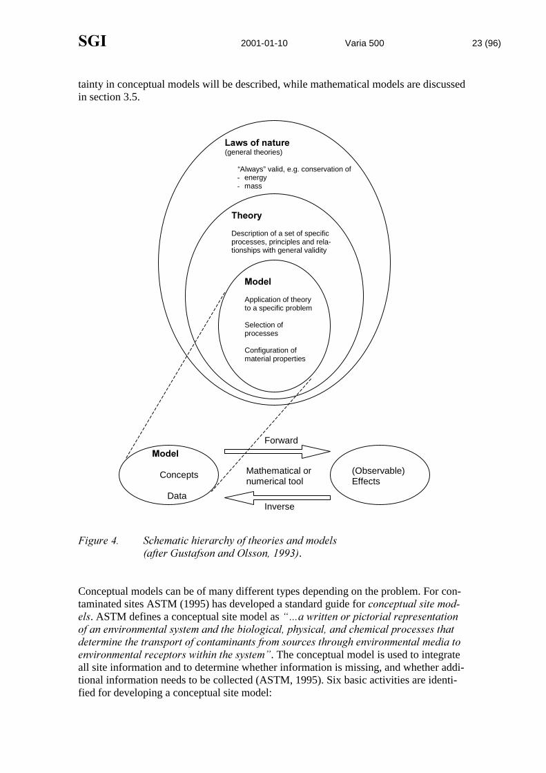
6*, 2001-01-10 Varia 500 23 (96)

tainty in conceptual models will be described, while mathematical models are discussedin section 3.5.

)LJXUH�� 6FKHPDWLF�KLHUDUFK\�RI�WKHRULHV�DQG�PRGHOV�DIWHU�*XVWDIVRQ�DQG�2OVVRQ��.

Conceptual models can be of many different types depending on the problem. For con-taminated sites ASTM (1995) has developed a standard guide for FRQFHSWXDO�VLWH�PRG�HOV. ASTM defines a conceptual site model as ³«D�ZULWWHQ�RU�SLFWRULDO�UHSUHVHQWDWLRQRI�DQ�HQYLURQPHQWDO�V\VWHP�DQG�WKH�ELRORJLFDO��SK\VLFDO��DQG�FKHPLFDO�SURFHVVHV�WKDWGHWHUPLQH�WKH�WUDQVSRUW�RI�FRQWDPLQDQWV�IURP�VRXUFHV�WKURXJK�HQYLURQPHQWDO�PHGLD�WRHQYLURQPHQWDO�UHFHSWRUV�ZLWKLQ�WKH�V\VWHP´. The conceptual model is used to integrateall site information and to determine whether information is missing, and whether addi-tional information needs to be collected (ASTM, 1995). Six basic activities are identi-fied for developing a conceptual site model:

/DZV�RI�QDWXUH(general theories)

“Always” valid, e.g. conservation of- energy- mass

7KHRU\

Description of a set of specificprocesses, principles and rela-tionships with general validity

0RGHO

Application of theoryto a specific problem

Selection ofprocesses

Configuration ofmaterial properties

0RGHO

Concepts

Data

(Observable)Effects

Mathematical ornumerical tool

Inverse

Forward

6*, 2001-01-10 Varia 500 24 (96)

1. identification of potential contaminants2. identification and characterisation of the sources of contaminants3. delineation of potential migration pathways through environmental media4. establishment of background areas of contaminants for each contaminated medium5. identification and characterisation of human and ecological receptors6. determination of the limits of the study area or system boundaries

Uncertainties in the conceptual site model need to be identified so that efforts can betaken to reduce them. This is especially important for early versions of conceptual mod-els based on limited and incomplete information (ASTM, 1995). However, ASTM donot mention how this should be achieved in practice.

To perform some of the activities listed above, especially activity 3 and 6, it is neces-sary to take the geologic and hydrogeological conditions into account. A common wayto do this is to develop conceptual geologic or hydrogeologic models. A conceptual hy-drogeological model describes qualitatively how a groundwater system functions(Koltermann and Gorelick, 1996). Poeter and McKenna (1995) emphasise the impor-tance to work with a range of different interpretations of the subsurface to take the un-certainty into account. Similarly, a set of different conceptual models is often consid-ered when uncertainty are handled for radioactive waste disposal studies (Äikäs, 1993).Yuhr et al. (1996) points out the importance of considering geologic uncertainty in sitecharacterisation and ways to reduce it.

Uncertainty arises from the choice of conceptual model, including the assumptionsabout relevant physical processes (James and Oldenburg, 1997). These uncertainties canbe as important as the estimates of contaminant levels themselves. Whenever a modelbased on limited data is used, model assumptions take the place of data. This can in-creases the subjectivity at the loss of objectivity (Borgman et al., 1996a).

James and Oldenburg (1997) have investigated the uncertainty in transport parametervariance and site conceptual model variations for a large-scale 3-D finite differencetransport simulation of trichloroethylene concentrations using FOSM and Monte Carlomethods. To transform the actual site history and conditions into a numerical simulationsystem a conceptual model was defined. A set of four conceptual models was definedwith the purpose to take the FRQFHSWXDO�PRGHO�XQFHUWDLQW\ into account; one base caseand three variations of the base case. For each of the four conceptual models the sameset of parameter uncertainties (variances) were used for uncertainty analysis. The resultshows that large uncertainties in calculated contaminant concentrations arise from bothparameter uncertainty and choice of conceptual model. Especially important was un-certainty about the subsurface heterogeneity. Because of the large uncertainties, a con-clusion is that predicted contaminant concentrations should always include estimates ofuncertainty. James and Oldenburg (1997) point out that uncertainty in the numericalsimulation model was not considered in the study, only parameter uncertainty and con-ceptual model uncertainty.

�� &RPELQLQJ�KDUG�DQG�VRIW�LQIRUPDWLRQ

A conceptual model are qualitative in nature but can be developed into some kind ofquantitative model by combining hard and soft information. Depending on the problem

6*, 2001-01-10 Varia 500 25 (96)

many different types of quantitative models are used, e.g. for hydrogeological simula-tions or contaminant transport simulations.

Koltermann and Gorelick (1996) reviewed techniques for incorporating geological in-formation in models for generating maps of hydraulic properties in sedimentary depos-its. They distinguish three different classes of models for this purpose: (1) structure-imitating methods, (2) process-imitating methods, and (3) descriptive methods. 6WUXF�WXUH�LPLWDWLQJ�PHWKRGV try to imitate the geometry of spatial patterns in the geologicmedia by techniques like spatial statistics, correlated random fields, probabilistic rulesetc. 3URFHVV�LPLWDWLQJ�PHWKRGV try to model the important processes. This can beachieved by using aquifer models and geologic process models. 'HVFULSWLYH�PHWKRGVcombine site-specific data and regional data with a conceptual geologic model. The aq-uifer is divided into zones and parameter values are assigned to each zone depending onthe conceptual geologic model and available measurements. A consequence of this isthat some of the descriptive methods are GDWD�GULYHQ, i.e. they are heavily based on site-specific measurement. Others are LQWHUSUHWDWLRQ�GULYHQ, i.e. they are primarily based onqualitative geologic information (Koltermann and Gorelick, 1996). Some models canincorporate soft information fairly well, while others are unable of doing that. As anexample, indicator-based methods allow great flexibility to include hard and soft data.Including soft information is often critical because hard data are often sparse(Koltermann and Gorelick, 1996).

Bayesian methods have been increasingly used for site characterisation during the lastdecade. McLaughlin et al. (1993) applied these techniques to characterise a coal tar dis-posal site. The strategy they used consists of four steps. First, a probabilistic descriptionof the natural heterogeneity in the subsurface is made. Second, prior statistics describingthe geological properties, hydraulic variables, and contaminant concentrations are de-rived. The prior statistics are used in a solute transport model to make a prior estimate.Third, a procedure is developed to update the prior statistics with field data. Finally, asequential program of data collection and updating is carried out, resulting in better andbetter characterisation of the subsurface.

Freeze et al. (1990) transform a conceptual model into a JHRORJLFDO�XQFHUWDLQW\�PRGHOand a SDUDPHWHU�XQFHUWDLQW\�PRGHO by incorporating the uncertainties. These models areused together with a�K\GURJHRORJLFDO�VLPXODWLRQ�PRGHO to take the uncertainties in geol-ogy and in parameter values into account by Bayesian updating.

Johnson (1996) used a similar approach and used Bayesian methodology to integratesoft information with hard data. Soft information of where contamination is likely to be,is used to develop a conceptual model. This image is updated with new sample data byindicator kriging.

Rosenbaum et al. (1997) discuss different probabilistic models for estimating lithology.They include geostatistics (indicator kriging and indicator cokriging), conditionalsimulation, and Bayes-Markov simulation.

6*, 2001-01-10 Varia 500 26 (96)

�� 8QFHUWDLQW\�LQ�TXDQWLWDWLYH�PRGHOV

A type of uncertainty that may be very important but often is overlooked is the uncer-tainty in the model itself, i.e. the model structure is the source of the uncertainty (seesection 2.3). As a typical example, this type of uncertainty could be the inherent uncer-tainty in the hydrogeological simulation model due to the fact that the model is a simpli-fication of reality. This uncertainty may be very difficult to quantify or separate fromother sources of uncertainty. A common name for it is PRGHO�XQFHUWDLQW\ (Morgan andHenrion, 1990) and this is also the name used in this report. Both qualitative and quan-titative models are affected by model uncertainty. Qualitative models are often equiva-lent to conceptual models and the uncertainty associated with these models has alreadybeen discussed. The quantitative models, on the other hand, can be of different nature.Typical examples include PDWKHPDWLFDO�PRGHOV, QXPHULFDO�PRGHOV, and VSDWLDO�VWDWLVWL�FDO�PRGHOV.

However, some authors define model uncertainty in other ways. Wagner (1999) andLacasse and Nadim (1996) use model uncertainty in the context of uncertainty in modelpredictions. The latter define model uncertainty as ³«WKH�UDWLR�RI�WKH�DFWXDO�TXDQWLW\�WRWKH�TXDQWLW\�SUHGLFWHG�E\�D�PRGHO´. This is an important difference in definition sincethe uncertainty in model predictions also includes all introduced uncertainty in data in-put (an ideal model that models reality correctly may still give imprecise predictions ifdata are uncertain). With the definition according to Lacasse and Nadim (1996) themodel uncertainty can be expressed with the concepts of bias and precision by calcu-lating the ratio of the actual quantity to the quantity predicted by the model. A meanvalue different from 1.0 expresses bias in the model, while the precision can be ex-pressed by the standard deviation of the model predictions.

Lacasse and Nadim (1996) argue that it is absolute more rational to include model un-certainty than to ignore it. Model uncertainty is generally large but it can be reduced.They describe how model uncertainty can be included in a geotechnical calculationmodel. Examples of how to evaluated model uncertainty is to compare model tests withdeterministic calculations, pooling of expert opinions, results from literature, and engi-neering judgement. For a qualitative understanding of model uncertainty they identifyand list factors of influence on model uncertainty.

Sturk (1998) recognises three causes for modelling uncertainty; (1) SURIHVVLRQDO�XQFHU�WDLQW\, (2) VLPSOLILFDWLRQV, and (3) JURVV�HUURUV. Professional uncertainty arises becauseof lack of knowledge of the studied phenomenon. Simplifications are introduced inmodels to make them less complex. Gross errors result because of omissions or lack ofcompetence.

Russell and Rabideau (2000) evaluated the importance of e.g. model complexity in arisk-based decision analysis framework, see section 6.4.4

In practice, model uncertainty and parameter uncertainty often overlap (Taylor, 1993).Sometimes, it is possible to construct a model in such a way that model uncertainty isconverted to uncertainty about parameter values. Such an approach often simplifies theanalysis. In situations when a phenomenon is modelled by different models, Morganand Henrion (1990) argue that it is inappropriate to assign probabilities to the differentmodels. Rowe (1994) comes to the same conclusion and states that probability has nomeaning here.

6*, 2001-01-10 Varia 500 27 (96)

Knopman and Voss (1988) developed a methodology for comparing different models(PRGHO�GLVFULPLQDWLRQ) based on error in contaminant transport model predictions. Theerror is quantified by regression analysis. They define a model error vector as:

56((( +=

where (6 is systematic error and (5 is random error. The systematic error is introducedwhen the physical system is described with an incorrect mathematical description. Thesource of random errors is measurement errors and inability of the model to capturestochasticity in the physical system. The model error may be in three forms; (1) over-specification, (2) underspecification, and (3) misspecification of the mathematicalstructure approximating the true system.

*HRVWDWLVWLFDO�PRGHOOLQJ includes several techniques, such as variogram analysis and anumber of different kriging methods. Estimation errors may be introduced in differentways such as; insufficient number of samples, sample data of poor quality that do notrepresent the actual concentrations, and poor estimation procedures (Myers, 1997). Ki-tanidis, as referred by Koltermann and Gorelick (1996), notes that YDULRJUDPV are oftencalculated and used without regard for the uncertainty in their parameters, i.e. the vario-grams are considered deterministic. To take the uncertainty of a variogram into accounta single, deterministic variogram should not be used; instead a set of variogram modelsthat fit the experimental data should be used.

Deutsch and Journel (1998) discuss the uncertainty about uncertainty models used instochastic simulation. They recommend sensitivity analysis to be used for model pa-rameters, especially decision variables, but also parameters such as the variogram range.

Dagdelen and Turner (1996) conclude that NULJLQJ is likely to lead to misinterpretationof the extent and degree of contamination at a site when it is applied without considera-tion of geological complexity. They discuss some aspects of this problem.

6*, 2001-01-10 Varia 500 28 (96)

�� 6$03/,1*�81&(57$,17<

�� ,QWURGXFWLRQ

The result of a site-investigation depends on samples of good quality. However, it isoften extremely difficult to obtain quality and reproducible samples and the require-ments to achieve sampling correctness are not widely known (Myers, 1997). Therefore,major sampling errors often occur. Maps of spatial contamination are often based on theassumption that the available data are reliable, which is often not the case, so one issimply mapping an illusion provided by the available data (Myers, 1997). This may, ofcause, affect the remedial decision and have a negative impact on both the economicsand the quality of the site cleanup. There are different ways of approaching this prob-lem. One is by using sampling theory developed by Pierre Gy to assist in the search andextraction of mineral resources. This theory, and other ways of handling sampling un-certainty for environmental applications, will be described in this chapter.

Typically, the error arising from field sampling is much larger than that associated withpost-sampling activities, such as sample preparation and chemical analysis (Crépin andJohnson, 1993). Sampling is an integral part of the measurement process that is oftenneglected in terms of the errors it generates (Ramsey et al., 1995). In practice there aretwo questions that generally arise:

1. How many samples should be taken?2. Where should the samples be located?

Uncertainties related to these and other sampling questions are addressed in this chapter.

�� 6DPSOLQJ�NH\�WHUPV

When the sampling literature is reviewed it becomes clear that an agreed terminology islacking. An author may use the word “sample” in one context, while other authors mayhave a different definition. As an example, the soil volume analysed at a laboratory mayhave at least the following different names: VDPSOH, DQDO\VLV�VDPSOH, VXEVDPSOH, WHVWSRUWLRQ, DOLTXRW� or VSOLW. Pitard (1993) and Myers (1997) present extensive lists of keyword explanations related to sampling. These are based on the particulate sampling the-ory presented in section 4.7. Other important sampling terms can be found elsewhere,e.g. in Keith (1996). The European Committee for Standardization (CEN) also definesseveral sampling key terms during its present standardisation work.

It is very important to understand the concepts of WDUJHW�SRSXODWLRQ, VDPSOHG�SRSXODWLRQ�VDPSOH�GRPDLQ�� and�VDPSOH. If they are not clearly defined and related to the objectiveof the investigation, the data collection may contain little useful information (Myers,1997). The target population is the real population of interest. When the target and sam-pled populations are not the same, there is a potential for biased results (Chai, 1996), i.e.sampling from mixed domains must be avoided.

Myers (1997) makes a distinction between VDPSOLQJ�VWUDWHJ\ and VDPSOLQJ�SODQ. Sam-pling strategy is a standardised set of goals and conditions that provide for correct sam-ple design, correct sample collection, and correct spatial assessment. A sampling planon the other hand, is a unique set of goals and conditions developed for a particular site.Therefore, a sampling plan can never be standardised, in contrast to a sampling strategy.

6*, 2001-01-10 Varia 500 29 (96)

�� 6DPSOLQJ�REMHFWLYHV

The literature about soil sampling is extensive but Huesemann (1994) identifies at leasttwo major limitations regarding it. Either the sampling publication is to statistically so-phisticated to be understood by an average scientist or engineer, or the document is tooconcerned with generalities such as QA/QC procedures (see section 4.4). Another limi-tation that is addressed is the difficulty to find a sampling publication that matches one´sVDPSOLQJ�REMHFWLYH and specific needs. In the literature it is relatively rare to find discus-sions about different sampling objectives. However, before measurements can be made,the concept of the problem to be solved and the model to be followed for its solutionmust be reasonably clear (Taylor, 1996). Koerner (1996) states that to collect a repre-sentative sample successfully, one must first clearly define the objectives of the sam-pling exercise. The most commonly mentioned sampling objectives appear to be:

1. to determine the average site contamination level (mean concentration)2. to classify the soil in different concentration classes during, or prior to, remediation3. to locate “hot spots”4. to delineate the contaminated area/plume5. to create a contour map (isopleth) over contaminant concentrations6. to forecast the contamination level during excavation (i.e. the concentration that can

be expected as excavation proceeds)7. to determine which chemical substances are present8. to monitor concentration changes over time

Scientific or statistically sound methods to reach several of these, and similar samplingobjectives, are described in the environmental literature. In practice, several other, andsometimes less stringent, sampling objectives exist. One is to get a rough estimate aboutthe concentration level at a site (Huesemann, 1994). This objective is a rather subjectiveone, but in practice it is used quite commonly. Such vague sampling objectives makedata evaluation problematic. Taylor (1996) mentions a question that is commonly askedbut cannot be answered by sampling: $UH�DOO�PHPEHUV�RI�WKH�SRSXODWLRQ�ZLWKLQ�DFFHSW�DEOH�OLPLWV" To answer this and similar questions the whole population has to be ana-lysed.

Several authors, e.g. Shefsky (1997), emphasise the importance of clearly stating thesampling objective in quantitative terms. Action or decision concentrations should bespecified with demands on the level of precision that is required.

In the following sections (4.4-4.8) some aspects that are common to several samplingobjectives will be described. They include; quality aspects and uncertainties in the plan-ning phase, which sampling pattern to use, sampling theories, especially the particulatesampling theory of Pierre Gy, and composite sampling. After that, uncertainty associ-ated with some of the eight sampling objectives listed above will be described (section4.9-4.11). These include:

� Sampling to estimate mean concentrations. This is relevant for sampling objectivenumber 1 and 2 above.

� Sampling to detect hot spots (sampling objective 3).

6*, 2001-01-10 Varia 500 30 (96)

� Sampling to delineate contaminated areas. This is relevant for sampling objective 4and 5.

Sampling objective 6-8 will not be addressed further. Sampling objective 2 (classifica-tion of soil in concentration classes) will not be discussed explicitly. Such methods aredescribed by for example Naturvårdsverket (1997).

�� 3ODQQLQJ�SKDVH��'42V�DQG�4$�4&�

'DWD�4XDOLW\�2EMHFWLYHV (DQOs) and 4XDOLW\�$VVXUDQFH�4XDOLW\�&RQWURO (QA/QC)systems consist of protocols and procedures for sampling and analysis that should befollowed to keep the uncertainty at acceptable level. Many of the procedures in DQOsand QA/QC are qualitative in nature, although quantitative advice sometimes is pre-sented. These concepts and procedures are developed by U.S. EPA and are presented ina number of guidelines and reports. A thorough discussion of QA/QC samples is givenby for example van Ee et al. (1990), who also provide QA methods and equations forquantification of total measurement error.

TotalStudy Error

SamplingDesign Error

MeasurementError

Inherentvariability

SamplingDesign

Sampling Frame Selection

Sampling Unit Definition

Selection Probabilities

Number of Samples

Physical SampleCollection

SampleHandling

Analysis

Support Volume/mass

Sample Delineation

Sample Extraction

Preservation

Packing

Labeling

Storage

Transport

Preparation

Subsampling

Extraction

Analytical Determination

Data Reduction

)LJXUH�� $Q�H[DPSOH�RI�KRZ�7RWDO�6WXG\�(UURU�FDQ�EH�EURNHQ�GRZQ�E\�FRPSR�QHQWV��DIWHU�8�6��(3$��

6*, 2001-01-10 Varia 500 31 (96)

The DQO process (U.S. EPA, 1994) is a planning approach to develop sampling de-signs for data collection activities that supports decision-making. The system should beused on a project level but it is not mandatory to follow the DQO in the U.S. EPA qual-ity system. The process is iterative. The DQO enables evaluation of two opposing con-ditions, such as if a site should be regarded as contaminated or not. The outcome of theDQO process is a sampling design for collecting data, including the number of samplesto collect, where and how to collect them, and acceptable limits on the probability ofdecision errors. The DQO process can be summarised as (Robbat, 1996):

1. State the problem2. Identify the decision to be made3. Identify the inputs to the decision4. Define the boundaries of the study5. Develop decision rules6. Specify tolerable limits on decision errors7. Optimise the conceptual model

In step 5, the choice of a statistical decision rule is encouraged. Two types of decisionerrors are considered in step 6; false acceptance and false rejection. In this step the TotalStudy Error is broken down into sampling design errors and measurement errors ac-cording toFigure 5.

Computer software related to the DQO process is presented in the appendix. A frame-work for integration of the DQO process with SDUWLFXODWH�VDPSOLQJ�WKHRU\ (section 4.7)and geostatistics is presented by Myers (1997).

�� 6DPSOLQJ�SDWWHUQ�GHVLJQ

A great number of different sampling designs (sampling patterns) are described in theliterature. Here, the most common ones will be described briefly, mainly organised ac-cording to Gilbert (1987) (other authors uses a somewhat different classification). Adetailed presentation of sampling designs is also given by U.S. EPA (2000a). In thissection, our emphasis is on spatial sampling, although many of the described strategiescan also be applied on temporal sampling. Four basic ways of selecting sampling loca-tions can be distinguished:

1. Haphazard sampling2. Judgement sampling3. Search sampling4. Probability (statistical) sampling

In addition, K\EULG�VDPSOLQJ�SODQV (Taylor, 1996) is sometimes used, i.e. combinationsof the ones listed above. Taylor (1996) identifies a fifth type of sampling design that iscommonly used: SURWRFRO�VDPSOLQJ. This type of sampling follows specified legal orcontractually mandated plans. A common feature of the mentioned sampling strategiesis that they use a fixed sampling pattern. A different approach is the DGDSWLYH�VDPSOLQJstrategy (e.g. Cox, 1999; Johnson, 1996; Robbat, 1996), where the sampling is per-formed in stages and the information from one stage is used to locate the sampling

6*, 2001-01-10 Varia 500 32 (96)

points for the next stage. This approach usually accounts for patterns of variability bygeostatistics. Examples of adaptive sampling are presented in chapter 6. An innovativeand relatively unknown sampling design is the UDQNHG�VHW�VDPSOLQJ (U.S. EPA, 2000a).It combines simple random sampling with the field investigators professional judge-ment. The advantages are cost-efficiency and better estimates of mean concentrations.

In on-going work on sampling techniques for waste, the European Committee for Stan-dardization (CEN) uses a somewhat different classification of sampling designs. CENdifferentiate between SUREDELOLVWLF�VDPSOLQJ and PHWKRGRORJLFDO�VDPSOLQJ. Probabilisticsampling is statistically based, while methodological sampling is not. Two types ofmethodological sampling can be distinguished, LQIRUPDWLYH and QRQ�LQIRUPDWLYH. Infor-mative methodological sampling is probabilistic sampling from a subpopulation, re-sulting in partial representative samples. With non-informative sampling there is no wayof judging how representative a sample is.

During KDSKD]DUG�VDPSOLQJ the samples are taken with no systematic method in mindand the method should not be used (Huesemann, 1994). The philosophy behind haphaz-ard sampling is that “any sampling location will do”, but this assumption is highly sus-pect in environmental pollution studies (Gilbert, 1987). Thompson and Ramsey (1995)use the term FRQYHQLHQFH�VDPSOH�for a sample taken with no regard to representative-ness. Several authors have pointed out the uselessness of haphazardly taken soil sam-ples.

-XGJHPHQW�VDPSOLQJ is subjective sampling of population units selected by an individual(Gilbert, 1987). Taylor (1996) calls this strategy LQWXLWLYH�VDPSOLQJ while U.S. EPA(2000b) uses the term DXWKRULWDWLYH�VDPSOLQJ. If the individual is skilful this strategycan be successful but the result depends heavily on the personal judgement of the sur-veyor. However, there is no way to verify the result, except through additional randomsampling, and no estimation of error is possible (Crépin and Johnson, 1993; U.S. EPA,2000b). Therefore, judgement sampling should not be used to characterise the averagecontamination level at a site (Huesemann, 1994). Despite its drawbacks judgementsampling is often used in practice. Often, judgement sampling does not refer to usingprior information to design a sampling strategy. The use of prior information and expertopinion is clearly needed in many situations (Gilbert, 1987).

One type of sampling that often can be regarded as judgmental is SUHIHUHQWLDO�VDPSOLQJ.Goovaerts (1997) defines preferential sampling as when sampling locations³«DUH�QHL�WKHU�UHJXODUO\�QRU�UDQGRPO\�GLVWULEXWHG�RYHU�WKH�VWXG\�DUHD´. Some reasons for prefer-ential sampling may be; (1) restrictions in accessibility, (2) denser sampling in criticalareas, or (3) clustered samples to characterise short-range variability. Any preferentialsampling is likely to impact sample statistics (Goovaerts, 1997).

6HDUFK�VDPSOLQJ is a sampling strategy that is used to locate “hot spots”, plumes, orpollution sources. A sampling pattern is designed to find an object, of defined size andshape, with a specified probability of a hit. The method is based on search theory, whichcan be used to find the optimum spacing between sampling points and to minimise thenumber of samples. Often, prior information and expert judgement are used to designthe search-sampling plan. The validity of such a procedure depends on the accuracy ofprior information and on accurate measurements (Gilbert, 1987). A simplification in

6*, 2001-01-10 Varia 500 33 (96)

search theory is that the search objects is approximated as having simple shapes, oftencircular or ellipsoid shapes.

3UREDELOLW\�VDPSOLQJ refers to the use of a specific method of random selection (Gilbert,1987) and is based on probability theory. It can be used to estimate the average con-tamination level at a site. Another common name for this type of strategy is VWDWLVWLFDOVDPSOLQJ. In practice, random sampling is achieved only by following strict rules so thatall individual samples in a population are selected without bias. The most commonlyused probability sampling designs include:

� Simple random sampling� Stratified random sampling� Multistage sampling� Cluster sampling� Systematic sampling� Systematic random sampling� Double sampling

Four of these sampling designs are illustrated in Figure 6.

)LJXUH�� ,OOXVWUDWLRQ�RI�VRPH�SUREDELOLW\�VDPSOLQJ�GHVLJQV��DSSOLHG�WR�VSDWLDOVDPSOLQJ�

In VLPSOH�UDQGRP�VDPSOLQJ (or strict random sampling) the sample position is locatedrandomly, i.e. all personal bias relating to landscape position is avoided and each loca-tion has an equal probability of selection (Figure 6a). Simple random sampling is ap-propriate for estimating means and totals for the entire population, but only if the popu-lation does not contain major trends (Gilbert, 1987). For small (< 0.5 ha) and uniformlyaffected sites, as few as five to ten samples may be sufficient, while larger sites mayneed up to 25 samples. If a sufficient confidence level cannot be achieved with 25 sam-ples, the site should be divided into less variable units (Crépin and Johnson, 1993). It isimportant to note that random sampling is not equivalent to picking sampling locationshaphazardly (Gilbert, 1987). A major problem with simple random sampling is thatclusters tend to arise, which can lead to non-representative sampling (Myers, 1997).This can be avoided if systematic random sampling is used (see below).

a) Simple random sampling

b) Stratified random sampling

c) Systematic sampling

d) Systematic random sampling

6*, 2001-01-10 Varia 500 34 (96)

In VWUDWLILHG�UDQGRP�VDPSOLQJ the site is divided into a number of non-overlapping partsor subareas called strata, and within each strata sampling positions are located randomly(Figure 6b). The site can be divided into different strata based on expected differencesin contamination levels (Huesemann, 1994) or on geological grounds. The method ofstratified sampling can be used to (1) make statements about each strata separately, or(2) to increase the precision of population estimates by distributing the samples over theentire area. An advantage of the stratified random sampling is that the increased homo-geneity in each strata, increases sampling precision. Stratified sampling also makes itpossible to apply a number of statistical techniques (Crépin and Johnson, 1993).

In PXOWLVWDJH�VDPSOLQJ the population is divided into primary units and a set of primaryunits is selected by simple random sampling (Gilbert, 1987). Then, each sample is ran-domly subsampled (two-stage sampling). An example of two-stage sampling in con-taminated land investigations is the random collection of soil samples, followed by ran-dom selection of aliquots (test portions) from each soil sample.

Another definition of multistage sampling is when an area is sampled several times withdata evaluation performed between each stage. This strategy is similar to the adaptivesampling strategy. It results in better spatial definition of contaminants for a given sam-ple size (Ferguson, 1993). If two-stage sampling is performed, about half of the totalnumber of samples should be assigned to each stage, as a rule of thumb (Ferguson,1993). A more formal solution can be derived by Bayesian statistics.

&OXVWHU�VDPSOLQJ is where a cluster of individual units are chosen at random, and allunits in the cluster are measured (Gilbert, 1987). This sampling design is of little inter-est at contaminated sites and will not be discussed further.

In V\VWHPDWLF�VDPSOLQJ (or grid sampling)�the sampling points follow a simple patternand are separated by a fixed distance, usually in a regular grid (Figure 6c). Locatingsampling points in the field is easier with systematic sampling than with simple randomsampling. The first sampling point has to be located randomly and the rest of the gridshould be laid out according to that point. Random sampling can always be replaced bysystematic sampling and tools like geostatistics can be applied (Crépin and Johnson,1993). Statistical studies indicate that systematic sampling may be preferred over othersampling plans for estimating means, totals and patterns of contamination (Gilbert,1987). Systematic sampling can also be used with a temporal pattern, i.e. samples canbe taken at specified time intervals.

One drawback of the systematic sampling is the loss in precision when the populationhas a periodic trend that corresponds to the sampling interval. One such example iswhen the contaminant has been transported along a drain parallel to the sampling grid.Also, the variance of estimated means and other quantities are more complicated to cal-culate than for simple random sampling (Gilbert, 1987).

6\VWHPDWLF�UDQGRP�VDPSOLQJ (or random sampling within blocks or segments) is a com-bination of random sampling and systematic sampling. It has the advantage of bothmethods and in many cases it is the method of choice (Huesemann, 1994). Randomsamples are taken within a systematic rectangular or square grid area (Figure 6d), i.e.the study area is better covered compared to simple random sampling. Systematic ran-

6*, 2001-01-10 Varia 500 35 (96)

dom sampling also has advantages over systematic sampling if systematic contamina-tion patterns are present at the site.

�� 6DPSOLQJ�WKHRULHV

Borgman et al. (1996b) distinguishes between two types of sampling theories:

1. design-based sampling (classical finite sampling theory), and2. model-based sampling

The main distinction between the two is that in model-based sampling a model is usedto account for patterns of variability within the population. One example of the model-based approach is when a geostatistical model is used to design the sampling. Model-based sampling is usually more effective than design-based sampling because it makesmore complete use of information about the population. In design-based (classical)sampling no assumption of the underlying population is made, which makes it funda-mentally objective (Borgman et al., 1996b). The theories to determine mean concentra-tions (section 4.9) and to detect hot spots (section 4.10) are examples of design-basedsampling.

A third sampling theory is available, except from the two mentioned: The particulatesampling theory of Pierre Gy. This theory will be described below.

�� 3DUWLFXODWH�VDPSOLQJ�WKHRU\

�� ,QWURGXFWLRQ

Although several articles and books about sampling have been written there is only onesampling theory that can be regarded as general and comprehensive. This sampling the-ory was developed by the French mining-engineer Pierre Gy in the 1960s, 1970s and1980s for the mining industry. The theory is applicable to the sampling of particulatematerials and fluids (Borgman et al., 1996b). Other theories only cover small parts ofthe sampling problem but Gy´s theory is the only theory of sampling of particulate ma-terial that is accepted and undisputed world-wide (Pitard, 1993). However, it is not evi-dent that the theory is applicable to all aspects of environmental sampling, for examplesampling of volatile organic compounds (VOC) (see section 4.7.7).

The theory has connections with both classical statistics and geostatistics (Borgman etal., 1996b). Geostatistical aspects of Gy´s theory are addressed by Flatman and Yfantis(1996) and Myers (1997). A improvement upon classical statistics is that the variouserror sources are directly addressed. The separation of error sources is an important as-pect because some errors may represent bias, not simple random variation (Borgman etal., 1996b). The various components of variance of this sampling theory sound triviallyobvious when pointed out, but they are easily overlooked (Flatman and Yfantis, 1996).Also, sampling theory shows that seemingly harmless assumptions may result in sub-stantial sampling errors (Myers, 1997).

Gy has presented his work in a number of French and English publications but the highcomplexity has restricted the use of his sampling theory by engineers and scientists. Amore accessible presentation of the theory is presented by Pitard (1993). Shorter pres-

6*, 2001-01-10 Varia 500 36 (96)

entations of the theory, with the focus on environmental sampling, are available in forexample Myers (1997), Shefsky (1997), Borgman et al. (1996b), Flatman and Yfantis(1996), and Mason (1992).

�� 6DPSOLQJ�HUURUV

According to the sampling theory by Pierre Gy there are seven basic sampling errors:

1. The Fundamental Error ()()2. The Grouping and Segregation Error (*()3. The Long-Range Heterogeneity Fluctuation Error (&(�)4. The Periodic Heterogeneity Fluctuation Error (&(�)5. The Increment Delimitation Error ('()6. The Increment Extraction Error ((()7. The Preparation Error (3()

These errors, together with the DQDO\WLFDO�HUURU $(, are components of the RYHUDOO�HVWL�PDWLRQ�HUURU 2(. For convenience the first six errors can be combined to shortenmathematical formulas; the VKRUW�UDQJH�KHWHURJHQHLW\�HUURU &(� (=)(�*(), the FRQ�WLQXRXV�VHOHFWLRQ�HUURU &( (=&(��&(��&(�), and the PDWHULDOLVDWLRQ�HUURU 0((='(�((). The following error sum relationships can be formulated:

Sampling Selection Error, 6(: 6(� �&(��0(Total Sampling Error, 7(: 7(� �6(��3(Overall Estimation Error, 2(: 2(� �7(��$(

TE AE

OE

PE SE

ME

EEDE

CE

CE2CE1 CE3

FE GEFundamentalError

Grouping andSegregation Error

PreparationError

Analytical Error

IncrementDelimitationError

IncrementExtractionError

Long RangeHeterogeneityFluctuation Error

PeriodicHeterogeneityFluctuation Error

Overall Estimation Error

Total Sampling Error

Sampling Selection Error

ContinuousSelection Error

MaterialisationError

)LJXUH�� ,OOXVWUDWLRQ�RI�WKH�UHODWLRQVKLSV�EHWZHHQ�GLIIHUHQW�W\SHV�RI�HUURUV��DF�FRUGLQJ�WR�3LHUUH�*\�V�VDPSOLQJ�WKHRU\�

6*, 2001-01-10 Varia 500 37 (96)

The relationship between the different errors is illustrated in Figure 7. The meaning ofthe basic sampling errors is not self-evident and is therefore explained below.

A key word in the sampling theory is sampling�FRUUHFWQHVV. A sample methodology isconsidered unbiased and correct if all of the particles in the sampling unit have exactlythe same probability of being included in the sample (Shefsky, 1997).

7KH�)XQGDPHQWDO�(UURU��)(�The fundamental error is an important error because it still remains when a samplingoperation is perfect. Since the fundamental error affects the measured concentration it iscritical to manage this error, and it is the only error that never cancels out. It is also theonly error that can be assessed independently of the sampling method (Borgman et al.,1996b).

The fundamental error is a statistical consequence of the particulate nature of geologicsamples (Shefsky, 1997), see also the Representative Elementary Volume in Figure 8.As defined by Gy, the fundamental error is the relative error in estimating the grade(grade of ore may be analogous to the percentage of some chemical present) (Borgmanet al., 1996b). It is caused by the range of particle sizes in the medium and the fact thatoften only certain sized particles contain the pollutant of interest (Flatman and Yfantis,1996). Also, the contaminant itself can exist as particles such as lead shots or paintchips, which may result in large fundamental errors as illustrated by Shefsky (1997). Onthe other hand, if all the contaminant particles are very small, the fundamental error willalso be small. Pitard (1993) provides equations and sampling nomographs for quantifi-cation of the fundamental error as a function of some physical properties. The most im-portant of these properties is the maximum particle size. Mason (1992) provides a prac-tical guide for determining the maximum and minimum variance of the fundamentalerror. A statistical basis of the fundamental error, with illustrative explanations, is pre-sented by Shefsky (1997). He also provides practical advice on how to avoid or reducefundamental error and bias in soil sampling.

It is important to note that a fundamental error is introduced at each stage of sampling.Therefore, repeated subsampling leads to accumulation of fundamental errors, whichquickly can exceed 50-100 % (Myers, 1997). Because only a small mass of soil usuallyis used in laboratory analysis, the stage of subsampling for the analytical sample is thestage most apt to unacceptable magnitude of the fundamental error (Flatman and Yfan-tis, 1996). Shefsky (1997) states that if ³«ZH�VXEVDPSOH�ZLWKRXW�DQ\�UHJDUG�WR�KRPRJ�HQLVDWLRQ�RU�SDUWLFOH�SURSHUWLHV��WKH�UHVXOW�ZLOO�EH�DQDO\WLFDO�GLVDVWHU´.

If a large fundamental error is present, the sample will not represent what is in the fieldand it may be a waste of time to spend money to make other errors small (Borgman etal., 1996a). The magnitude of the fundamental error increases when the constitutionheterogeneity (see section 4.7.3) increases (Flatman and Yfantis, 1996).

7KH�*URXSLQJ�DQG�6HJUHJDWLRQ�(UURU��*(�The grouping and segregation error results from the distribution heterogeneity (see sec-tion 4.7.3). The heterogeneity may be in density, particle size, shape, adhesion, cohe-sion, magnetism, affinity for moisture etc. so that the particles come together by groupsduring movement or vibration (Flatman and Yfantis, 1996). Under normal conditions

6*, 2001-01-10 Varia 500 38 (96)

this error has a non-zero mean. The variance of the grouping and segregation error canbe written as:

( ) ( ) ( ) ( ))(V)(V&(V*(VV

221

22 ξγ=−=

where γV is the grouping factor and ξ is the segregation factor. In practice there are threeways of minimising V��*(�:

1. To minimise the variance of the fundamental error V��)(�.2. To minimise the grouping factor γV. In practice, this may be the most effective way

to minimise the variance V��*(�.3. To minimise the segregation factorξ by homogenisation techniques. However,

Myers (1997) warns that homogenisation of heterogeneous material is often wishfulthinking and may instead promote segregation, e.g. by the gravity force. To avoidsuch errors, mechanical sampling splitting devices could be used (Shefsky, 1997).

Theoretically, this error grows larger without bounds if the size of the analytical sampleapproaches the size of the grains in the sample. The consequence of this is that whensubsampling is performed in the laboratory, the chemist can turn the analytic equipmentinto a random number generator if the sample material has not been prepared correctly(required fineness and correct subsampling procedure) (Flatman and Yfantis, 1996).

7KH�/RQJ�5DQJH�+HWHURJHQHLW\�)OXFWXDWLRQ�(UURU��&(��This error is due to the long-range heterogeneity K� described in section 4.7.3. It is gen-erated by local trends. The variance of this error, V��&(��, can be quantified by thevariogram of geostatistics.

7KH�3HULRGLF�+HWHURJHQHLW\�)OXFWXDWLRQ�(UURU��&(��This error is introduced by cyclic phenomena. It is a non-random error generated byheterogeneity K� (see section 4.7.3).

7KH�&RQWLQXRXV�6HOHFWLRQ�(UURU��&(�The continuous selection error is the sum of the four errors above ()(�*(�&(��&(�).It is regarded as the result of the total heterogeneity contribution K (see section 4.7.3)and is the sum of errors generated by the process of material selection during sampling.

7KH�0DWHULDOLVDWLRQ�(UURU��0(�Many of the errors introduced by heterogeneity are typically random errors. Materiali-sation errors, on the other hand, are almost always biased and are probably the majorcause of all biases in sampling (Myers, 1997). The materialisation error is the sum ofthe LQFUHPHQW�GHOLPLWDWLRQ�HUURU ('() and the LQFUHPHQW�H[WUDFWLRQ�HUURU ((().

The LQFUHPHQW�GHOLPLWDWLRQ�HUURU results from an incorrect shape of the volume delim-iting the increment (in soil sampling an increment is the physical piece of soil removedfrom the ground and from which the sample is taken). Incorrect shape of the delimita-tion tool (sampling device) can lead to unequal probability for material to be part of theincrement, i.e. the concept of equiprobability in all directions is violated. A shovel witha round shape is an example of a sampling device that causes a delimitation error. Theshovel will preferentially collect material from the top of the lot, with less material ex-tracted from the bottom. This introduces a delimitation error and a bias.

6*, 2001-01-10 Varia 500 39 (96)

The LQFUHPHQW�H[WUDFWLRQ�HUURU results from an incorrect extraction of the increment.The extraction is said to be correct if all particles with their centre of gravity within theboundaries of the increment will belong to the increment. Depending on the construc-tion of the sampling device and how the sampling is performed, these particles may notbe extracted as a part of the increment, or particles outside the domain of the incrementmay be collected. This increment extraction error is often different from zero and istherefore an important source of sampling bias.

Myers (1997) points out that most of the sampling devices available for environmentalsampling are incorrect. Examples of such devices are augers, thiefs, and triers. If a cyl-inder could be cut out exactly in the material by a laser and then taken out intact bylevitation as in science fiction, these two errors could be avoided (Flatman and Yfantis,1996).

7KH�6DPSOLQJ�6HOHFWLRQ�(UURU��6(�The sum of &( and 0( is the VDPSOLQJ�VHOHFWLRQ�HUURU. The mean of 6( is what usuallyis called sampling bias. If the mean of 6( is zero the sample is said to be unbiased, al-though this case is never encountered in practice (Pitard, 1993). A sample is said to beaccurate when the mean of 6( is smaller than a certain standard of accuracy.

7KH�3UHSDUDWLRQ�(UURU��3(�All the previously described errors are selective while the preparation error is non-selective. The preparation can consist of a number of stages, such as comminution(grinding, crushing and pulverising), screening, mixing, drying, filtration, weighing,packing etc. (Pitard, 1993). Different types of errors can be introduced during prepara-tion:

� &RQWDPLQDWLRQ�HUURUV, due to improper procedures, contaminated equipment, dustproblems etc.

� /RVV�HUURUV, especially for volatile organic compounds if improper sampling, stor-age, and handling procedures are employed.

� $OWHUDWLRQ�RI�FKHPLFDO�FRPSRVLWLRQ. This error is related to loss errors and includesfor example degradation of chemical substances in the sample.

� 8QLQWHQWLRQDO�PLVWDNHV. Common examples of unintentional mistakes include drop-ping samples, mixing labels, mixing fractions from different samples, contaminationetc. This error can be reduced if the personnel are skilled.

� 6DERWDJH�DQG�IUDXG. This type of error may be rare but the possibility for it still ex-ists.

7KH�$QDO\WLFDO�(UURU��$(�This error is not part of the sampling error and is described in section 5.3. It does notinclude the selection of the subsample to be analysed. The error in subsampling shouldbe a part of the total sampling error 7(.

7KH�2YHUDOO�(VWLPDWLRQ�(UURU��2(�The overall estimation error can be quantified as the sum of the variances of all sam-pling and analytical errors:

22222$(3(0(&(2(

σσσσσ +++=

6*, 2001-01-10 Varia 500 40 (96)

Usually, several stages of sampling (subsampling) and preparation are performed priorto analysis. If all types of errors are taken into account the overall estimation error canbe expressed as (Pitard, 1993):

( )∑=

+++++++=1

Q

QQQQQQQ(('(&(&(*()(3($(2(

132

where N is the number of sampling or preparation stages. There are some importantaspects of this expression; (1) there are many different types of errors to consider, (2)errors are introduced in all stages of sampling, preparation and analysis, and (3) the er-rors are additive. Because sampling is performed in stages, most of the errors can enterthe problem many times and the stage with the greatest error will form the lower boundon the overall estimation error (Borgman et al., 1996b).

�� +HWHURJHQHLW\

Myers (1997) and Pitard (1993) comment that homogeneity is in fact an illusion. In-stead, heterogeneity constitutes a fundamental part of sampling theory. Two basic typesof heterogeneity can be distinguished: &RQVWLWXWLRQ�+HWHURJHQHLW\ and 'LVWULEXWLRQ�+HW�HURJHQHLW\. The constitution heterogeneity is caused by the fundamental properties ofthe particles, i.e. the inherent variability in composition of each particle. This type ofheterogeneity is fixed and homogenisation has no effect on it. The only way to reducethe constitution heterogeneity is by comminution where the properties of the particlesare changed. Constitution heterogeneity is the cause of the fundamental error FE.

A lot, such as a soil volume, can be visualised as separate groups of particles making upthe lot. Each group is composed of a certain number of particles with certain character-istics. The 'LVWULEXWLRQ�+HWHURJHQHLW\ is related to how the individual particles are rep-resented within the groups. It depends on three factors: (1) the constitution heterogene-ity, (2) the spatial distribution of particles, and (3) the shape of the lot. The distributionheterogeneity is responsible for the grouping and segregation error GE. It is also closelyrelated to the VXSSRUW�described in section 4.7.5. The distribution heterogeneity getssmaller when the support volume is increased and it is always smaller or equal to theconstitution heterogeneity (Pitard, 1993).

For practical applications, a model of heterogeneity K with three different kinds of het-erogeneity is suggested by Pitard (1993):

321 KKKK ++=

where:K� = the VKRUW�UDQJH�KHWHURJHQHLW\, typically random and discontinuous. It is influenced

by the constitution heterogeneity and the distribution heterogeneity. The short-range heterogeneity h1 is responsible for the sampling errors FE and GE. The vari-ance of the short-range heterogeneity is equal to σ��&(��.

K� = the ORQJ�UDQJH�KHWHURJHQHLW\ (or ODUJH�VFDOH�VHJUHJDWLRQ) reflects local trends, usu-ally non-random and non-cyclic. Its variance is equal to σ��&(��.

6*, 2001-01-10 Varia 500 41 (96)

K� = the SHULRGLF�KHWHURJHQHLW\ reflects cyclic phenomena. This heterogeneity is mostcommon in flowing streams of material, such as water. Its variance is equal toσ��&(��.

The effect of short-range and long-range heterogeneity is illustrated in Figure 8. Myers(1997) presents methods to characterise the heterogeneity K and to estimate optimumsample weights.

A concept closely related to heterogeneity, but not addressed in particulate samplingtheory, is DQLVRWURS\. A medium is said to be anisotropic with respect to a certain prop-erty if that property varies with direction (Bear, 1988). This concept is very importantfor a property like hydraulic conductivity, but also for contaminant concentrations insoil or groundwater. Anisotropic contamination at a site can be handled by geostatistics,which are not included in the particulate sampling theory. However, Myers (1997) inte-grates sampling theory and geostatistics into the concept of Geostatistical Error Man-agement (GEM).

�� 5HSUHVHQWDWLYHQHVV

One objective in a typical site-investigation is to collect “representative” samples. How-ever, the term UHSUHVHQWDWLYH is always loosely defined in qualitative terms, i.e. it is aqualitative parameter (Myers, 1997). Several definitions of representativeness exist.Koerner (1996) gives the following definition: ³$�UHSUHVHQWDWLYH�HQYLURQPHQWDO�VDPSOHLV�RQH�WKDW�LV�FROOHFWHG�DQG�KDQGOHG�LQ�D�PDQQHU�WKDW�SUHVHUYHV�LWV�RULJLQDO�SK\VLFDOIRUP�DQG�FKHPLFDO�FRPSRVLWLRQ�DQG�WKDW�SUHYHQWV�FKDQJHV�LQ�WKH�FRQFHQWUDWLRQ�RI�WKHPDWHULDOV�WR�EH�DQDO\VHG�RU�WKH�LQWURGXFWLRQ�RI�RXWVLGH�FRQWDPLQDWLRQ´. Chai (1996)defines representative sampling as ³«D�SURFHVV�E\�ZKLFK�D�VHW�RI�VDPSOHV�LV�REWDLQHGIURP�D�WDUJHW�SRSXODWLRQ�WR�FROOHFWLYHO\�PLUURU�RU�UHIOHFW�FHUWDLQ�SURSHUWLHV�RI�WKHSRSXODWLRQ´. Taylor (1996) states that it is virtually impossible to demonstrate repre-sentativeness. In fact, “representative samples” are often used to make decisions eventhough no real evidence is presented to verify that the sample represents anything butitself.

Sampling theory goes one step further and provides a quantitative definition of the rep-resentativeness of a sample. A sample is regarded as representative when the meansquare error of the sample selection error, U�(6(�, is smaller than a specified standard U�

�

(Myers, 1997):

( ) ( ) ( ) 20

222 U6(6(P6(U ≤+= σ

�� 6DPSOH�6XSSRUW

When characterising a geologic or environmental area the physical size of the samplingunit is very important and must be specified. This concept is known as VXSSRUW(Koltermann and Gorelick, 1996; Myers, 1997). The support in soil sampling is definedas the size, shape, and orientation of the physical sample taken at a sample point. Theconcept is closely related to the nugget effect in geostatistics (Starks, 1986). Flatmanand Yfantis (1996) define support as a larger volume that the sample is supposed to rep-resent, often the remediation unit. The support can be illustrated with the concept of5HSUHVHQWDWLYH�(OHPHQWDU\�9ROXPH (REV) used in the field of hydrogeology (Figure 8).

6*, 2001-01-10 Varia 500 42 (96)

The change in measured value when the volume increases is a result of heterogeneity atdifferent scales (see section 4.7.3), and the REV is the volume where the large fluctua-tions cease (Bear, 1979).

Microscopic Macroscopic

Heterogeneous

Homogeneous

V5V4V3V2V100

1

n

Volume

)LJXUH�� ,OOXVWUDWLRQ�RI�WKH�5HSUHVHQWDWLYH�(OHPHQWDU\�9ROXPH��5(9��DSSOLHG�WRSRURVLW\�DW�WKH�PLFURVFRSLF�DQG�PDFURVFRSLF�VFDOH��DIWHU�+XEEHUW�LQ)UHH]H�DQG�&KHUU\��7KH�5(9�LV�HTXDO�WR�WKH�YROXPH�9��

If the support is not specified, a statement of a population of measured concentrationshas no meaning. Myers (1997) gives the following example of a statement that ismeaningless unless the support is specified: ³7KH�FRQFHQWUDWLRQV�RI�OHDG�DW�WKH�VLWH�IRO�ORZ�D�ORJQRUPDO�GLVWULEXWLRQ��ZLWK�D�PHDQ�RI��SSP�DQG�D�VWDQGDUG�GHYLDWLRQ�RI��SSP�´ This statement is only valid for one specific sample support. If the support ischanged the statement will most probably be incorrect.

Another way of describing to concept of support is as follows: A sample point is seldomlocated exactly. Often, the sampling team may miss the point by several meters. Thesupport should be chosen in such a way that error variance due to misses will be small(Starks, 1986). Samples with smaller support volumes have higher variances and to re-duce the variance the support can be increased. One way of increasing the support is toincrease the diameter of the sample (core), but this is often impractical. A better methodis to take several samples in the vicinity of the designed sample point. Starks (1986)suggests taking the samples in a square grid around the sampling point, while Jenkins etal. (1996) used a 20 cm wide “sampling path” of circular shape. Each sample is thenanalysed, or compositing (see section 4.8) of all samples could be performed to savecost.

The support volume has important implications for estimation of the volume of con-taminated material for remediation. It is tempting to estimate the volume based on thesampling distribution of concentrations but such an approach can lead to serious esti-mation errors and high unexpected cost. Myers (1997) describes how the support vol-

6*, 2001-01-10 Varia 500 43 (96)

ume influences the variance of the sampling distribution curve. Any change in supportmust be checked using a nomogram made up for the specific site (Flatman and Yfantis,1996). If the support volume increases the variance decreases. Myers (1997) presentstwo methods to correct for small sample support; the�DIILQH�FRUUHFWLRQ and the�LQGLUHFWORJQRUPDO�FRUUHFWLRQ.

�� 'LPHQVLRQ�RI�ORWV

An important concept in the particulate sampling theory is the dimension of the lot to besampled. Lots can be classified as zero-, one-, two- or three-dimensional lots (Pitard,1993). One example of a ]HUR�GLPHQVLRQDO�ORW is randomly distributed coloured balls ina jar, i.e. a lot that is considered a statistical population. A RQH�GLPHQVLRQDO�ORW could bea stream of water or material on a conveyor belt. The one-dimensional lot always has alinear or chronological behaviour (Pitard, 1993). An example of a WZR�GLPHQVLRQDO�ORW isa piece of flat contaminated land where the depth of the lot is small compared to theareal extent. 7KUHH�GLPHQVLRQDO�ORWV�are for example piles of material, truckloads, or soilunits where the thickness is not negligible.

It is possible to perform statistically correct sampling only from zero- and one-dimensional lots. Acceptable sampling is possible for two-dimensional lots under fa-vourable conditions but it is practically impossible to collect correct samples for three-dimensional lots, except in liquids (Myers, 1997). However, it is always possible to di-vide a three-dimensional lot into a series of two-dimensional strata.

Derived equations in the sampling theory (Myers, 1997; Pitard, 1993) are primarily ap-plicable to zero- and one-dimensional lots. Two- and three-dimensional lots requiregeostatistical techniques.

�� $SSOLFDWLRQ�WR�HQYLURQPHQWDO�SUREOHPV

One of the key concepts of Gy´s theory is that one can work with the particle size (bygrinding) and the sample weight in order to reduce the variance to an acceptable level(Mason, 1992).The theory was not developed for environmental problems but many aspects of the the-ory are still relevant for such problems. However, for certain environmental problemsthe theory may still be incomplete. For quantification of the fundamental error one im-portant parameter is the maximum particle size of the medium. If the pollutants areheavy metals grinding will (probably) not alter the chemical composition but for volatileor semi-volatile chemicals this technique is inappropriate. However, most soils do notrequire grinding unless gravel, cobbles, or other large components are present (Mason,1992).

The extension of the theory to volatile or semi-volatile chemicals is an undeveloped partof environmental sampling (Flatman and Yfantis, 1996). Further discussion on thismatter can be found in Mason (1992).

�� &RPSRVLWH�VDPSOLQJ

The process of compositing is a physical averaging of the material used to form thecomposite sample. Samples are taken from different locations and then mixed to in-

6*, 2001-01-10 Varia 500 44 (96)

crease sample support (Shefsky, 1997). The measured value for a composite sampleshould be similar to the arithmetic mean of the measured values from the individualsamples forming the composite sample (Fabrizio et al., 1995). For bulk populations,such as soil and water, Gilbert (1987) provides statistical methods for composite sam-pling. Fabrizio et al. (1995) describe procedures for formation of composite samplesfrom segmented populations, i.e. populations with identifiable units such as fish etc.

G. Lovision et al. identified five stages of composite sampling (Fabrizio et al., 1995):1. identification of the target population2. statistical sampling3. compositing (the actual formation of composite samples)4. subsampling5. measurement

Compositing is an effective way to reduce intersample variance caused by the heteroge-neous distribution of contaminants (Jenkins et al., 1996). Another advantage of compo-siting is the cost-savings since only the composite sample need to be analysed. Myers(1997) points out that composite samples may save money but that they effectively wipeout any understanding of the long-range heterogeneity. They may be useful for calcu-lating average concentrations but not for spatial mapping of contaminants. Gilbert(1987) and Garner et al. (1996) provide equations for cost-effective strategies of de-tecting hot spots using composite sampling. U.S. EPA (2000a) provides practical infor-mation about composite sampling, as well as equations.

A problem when composite samples are used to estimate the mean concentration is thata certain amount of homogeneity must be assumed, otherwise the result cannot betrusted. Naturvårdsverket (1997) present a rule of thumb of when homogeneity in thesoil can be assumed (regarding contaminant concentrations). If the coefficient of varia-tion (CV = standard deviation/mean) is less than 1, composite samples can generally beused.

�� 0HDQ�FRQFHQWUDWLRQ�±�FODVVLFDO�DSSURDFKHV

�� 5DQGRP�VDPSOLQJ�XQFHUWDLQW\

The spatial heterogeneity at the sampling location is often quantified as�VDPSOLQJ�SUHFL�VLRQ� although this may not be in accordance with the sampling theory in section 4.7. Itcan be quantified by taking duplicate samples at some proportion of the sampling loca-tions, typically 10 % (Ramsey and Argyraki, 1997). This increases the sampling cost butenables quantification of sampling precision (but not sampling bias). Ramsey et al.(1995) found duplicate sampling to be a useful method for estimation of sampling preci-sion.

The random components of sampling uncertainty, expressed as variances, are additive(Taylor, 1996):

222

21

2QVDPSOLQJ VVVV K++=

where V�VDPSOLQJ�denotes the total random components of sampling variance, and V�� …V�Q are the components from sources � … Q, respectively. Taylor (1996) suggests that it

6*, 2001-01-10 Varia 500 45 (96)

may be difficult and time-consuming to quantify all random components of samplinguncertainty but that the overall value could be quantified by suitable experiments. Hesuggests taking at least seven replicate samples in a narrowly defined sampling areawhere the population variability is expected to be negligible. The equation above doesnot take population variability into account. To do this, Taylor (1996) suggests the fol-lowing relationship:

222SRSXODWLRQVDPSOLQJVDPSOH VVV +=

Jenkins et al. (1996) studied the short-range variability of contaminants at a samplinglocation. The site was contaminated by explosives. Seven discrete samples were col-lected at each sample location according to Figure 9. The sampling precision was de-scribed by classical statistic methods and the heterogeneity was found to be enormous atthe site. The conclusion was that random grab sampling without consideration of un-certainty may be totally inadequate for remedial decisions, although this strategy maybe appealing for its low cost (Jenkins et al., 1996). Composite samples on the other handresulted in good estimates with low standard deviation (see section 4.8).

2

1 36

5 4

7

1

d iameter 1 22 cm

)LJXUH�� ,OOXVWUDWLRQ�RI�VDPSOLQJ�VFKHPH�IRU�D�VKRUW�UDQJH�KHWHURJHQHLW\�VWXG\SHUIRUPHG�E\�-HQNLQV�HW�DO��6HYHQ�GLVFUHWH�VDPSOHV�ZHUH�FRO�OHFWHG�DW�HDFK�VDPSOH�ORFDWLRQ�

Most studies of spatial variability are performed at scales with sampling points rangingfrom meters to hundreds of meters apart. In contrast, Schumacher and Minnich (2000)studied the extreme short-range variability in VOC-contaminated soil. They found thatsoil properties (TCO, sand content and clay content) and contaminant concentrationsgenerally varied between 1 and 4 times at a distance of 15 cm (vertical direction). How-ever, extreme cases with concentration differences up to 43 times were noted. Theirfindings are closely related to the concept of sample support, as described in section4.7.5.

�� 6\VWHPDWLF�VDPSOLQJ�XQFHUWDLQW\

Systematic uncertainty, or bias, can be defined as the difference between the expectedvalue of a statistic and a population parameter. The following relationship can be for-mulated to illustrate bias (U.S. EPA, 2000b):

6*, 2001-01-10 Varia 500 46 (96)

E( += µ

where ( denotes the expected value of a sample average [, � denotes the true value ofinterest, and�E is the bias. Similar formulations of bias are given by Chai (1996). Hedistinguishes between three types of bias: (1) sampling bias, (2) measurement bias, and(3) statistical bias. The statistical bias is further divided into selection bias, statisticalbias in estimators, and bias in distribution assumptions.

Biased samples result from non-random sampling and from discriminatory sampling(Taylor, 1996). This happens if certain individuals in the sampled population are ex-cluded, i.e. the rule of equiprobability is violated. Mason (1992) divides factors thatcause sampling bias into two categories: LQWHQWLRQDO influences and DFFLGHQWDO influ-ences. One problem is that the bias may change over time. In sampling there is no suchthing as a constant bias (Pitard, 1993). Even when sampling is carried out in an idealway there will always be some sampling bias due to the particulate structure of mostmaterial. The bias may be negligible or very small but it is never strictly zero (Pitard,1993). Chai (1996) notes that sampling bias often cannot be measured because the truevalue � is typically not known.

Ramsey and Argyraki (1997) present four methods of estimating the PHDVXUHPHQW�XQ�FHUWDLQW\ at a contaminated site:

1. Single sampler/single protocol2. Single sampler/multiple protocol3. Multiple sampler/single protocol4. Multiple sampler/multiple protocol

In each method the uncertainty of the estimated mean concentration at the site is calcu-lated. In the multiple sampler methods (3 and 4), several different persons/organisationssample the site independently of each other and the variation in result is analysed. In themultiple protocol methods (2 and 4), different sampling plans (sampling pattern, num-ber of samples etc.) are used at the site. In Methods 2-4, the VDPSOLQJ�ELDV is estimatedto varying extent, but these methods demand extensive sampling. With method 2 thebias between different sampling protocols can be estimated. In method 3 the bias intro-duced by the sampler is estimated. Method 4 combines method 2 and 3. Squire et al.(2000) applied the multiple sampler/single protocol approach to estimate sampling biasat a synthetic reference sampling target.

The detection limit for sampling bias varies according to the JHRFKHPLFDO�YDULDELOLW\(see section 4.9.3) of the contaminant at the site (Ramsey et al., 1995). The greater thereal variation in concentration, the higher the detection limit of sampling bias.

Ramsey et al. (1999) demonstrated how sampling bias can be estimated by using a ref-erence sampling target, analogous to the use of a reference material for the estimation ofanalytical bias. However, it appears that their approach to sampling bias excludes biasintroduced by the sampling equipment and bias inherent in the sample according to Pi-erre Gy´s sampling theory.

6*, 2001-01-10 Varia 500 47 (96)

Van Ee et al. (1990) present a methodology to quantify sampling bias by quality as-sessment (QA) samples (see section 4.9.5).

Chang et al. (1998) demonstrates how sampling bias can be included in the estimationof total sampling uncertainty through the use of kriging and co-kriging techniques at asite where anisotropy exists. However, it appears that sampling bias introduced by thesampling technique is not considered in their work.

Barcelona (1996) points out that elements of the sampling operation may cause seriouserrors which cannot be treated strictly by statistics. Sources of such systematic errorsmay be sampling devices and handling operations. To identify and control such errors,documentation of sampling procedures in protocols is suggested. Koerner (1996) pro-vides a discussion of the effect of the sampling equipment.

Usually, the effort of reducing uncertainty in sampling is aimed at reducing the randomerrors. Therefore, the systematic errors in sampling are not widely known. Pitard (1993)emphasises this with the following words: ³7KH�GHVLUH�RI�FRQWUROOLQJ�DFFXUDF\�ZLWKRXWFRQWUROOLQJ�VDPSOLQJ�FRUUHFWQHVV�LV�FHUWDLQO\�WKH�ZRUVW�MXGJHPHQW�HUURU�WKDW�D�SHUVRQFDQ�PDNH��,W�LV�D�GLUHFW�GHSDUWXUH�IURP�ORJLF�´ He also points out that it can be mean-ingless to put much effort in estimation of sampling accuracy if there is a large bias.This is illustrated by the following words: ³0DQ\�DUH�WKRVH�ZKR�DUH�WHPSWHG�WR�WHVW�DQLQFRUUHFW�VDPSOLQJ�V\VWHP�IRU�LWV�DFFXUDF\´.

�� *HRFKHPLFDO�YDULDELOLW\��SRSXODWLRQ�YDULDELOLW\�

A type of uncertainty that is closely related to sampling uncertainty is the large scalevariability, also called JHRFKHPLFDO�YDULDELOLW\ (Ramsey and Argyraki, 1997), HQYLURQ�PHQWDO�YDULDELOLW\ (Clark et al., 1996), or the more statistically sound term SRSXODWLRQYDULDELOLW\ (Crépin and Johnson, 1993) (see also section 2.3). As is often the case withempirical quantities in the geologic environment, a scale problem is present. A contami-nant is never evenly distributed on a site, especially in soil. In the next section somemodels are presented where this type of uncertainty is one separable part of the totaluncertainty.

�� 0RGHOV�RI�WRWDO�UDQGRP�XQFHUWDLQW\

The total uncertainty is the sum of the contributions from random uncertainty and sys-tematic uncertainty (Taylor, 1996). Taking more samples, i.e. replicates, can reduce therandom uncertainty. The systematic component of uncertainty on the other hand (seesection 4.9.5), is independent of the number of replicates (Taylor, 1996). The total un-certainty includes not only sampling uncertainty but also other types of uncertainty, e.g.uncertainty in laboratory analysis (see chapter 5).

Ramsey and Argyraki (1997) use the term PHDVXUHPHQW�HUURU for the combined error ofsampling and analyses, including both random and systematic errors (note that meas-urement error sometimes refers only to analytical error). Crépin and Johnson (1993) usethe term PHDVXUH�YDULDELOLW\, in which they include sampling uncertainty, handling,transport and preparation uncertainty, subsampling uncertainty, lab uncertainty andbetween-batch uncertainty.

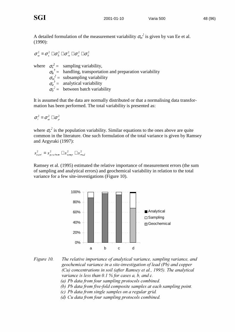
6*, 2001-01-10 Varia 500 48 (96)

A detailed formulation of the measurement variability σP� is given by van Ee et al.

(1990):

222222EDVVKVP

σσσσσσ ++++=

where σV� = sampling variability,

σK� = handling, transportation and preparation variability

σVV� = subsampling variability

σD� = analytical variability

σE� = between batch variability

It is assumed that the data are normally distributed or that a normalising data transfor-mation has been performed. The total variability is presented as:

222SPW

σσσ +=

where σS� is the population variability. Similar equations to the ones above are quite

common in the literature. One such formulation of the total variance is given by Ramseyand Argyraki (1997):

2222DQDOVDPSJHRFKHPWRWDO VVVV ++=

Ramsey et al. (1995) estimated the relative importance of measurement errors (the sumof sampling and analytical errors) and geochemical variability in relation to the totalvariance for a few site-investigations (Figure 10).

0%

20%

40%

60%

80%

100%

a b c d

Analytical

Sampling

Geochemical

)LJXUH�� 7KH�UHODWLYH�LPSRUWDQFH�RI�DQDO\WLFDO�YDULDQFH��VDPSOLQJ�YDULDQFH��DQGJHRFKHPLFDO�YDULDQFH�LQ�D�VLWH�LQYHVWLJDWLRQ�RI�OHDG��3E��DQG�FRSSHU�&X��FRQFHQWUDWLRQV�LQ�VRLO��DIWHU�5DPVH\�HW�DO��7KH�DQDO\WLFDOYDULDQFH�LV�OHVV�WKDQ��IRU�FDVHV�D��E��DQG�F��D��3E�GDWD�IURP�IRXU�VDPSOLQJ�SURWRFROV�FRPELQHG��E��3E�GDWD�IURP�ILYH�IROG�FRPSRVLWH�VDPSOHV�DW�HDFK�VDPSOLQJ�SRLQW��F��3E�GDWD�IURP�VLQJOH�VDPSOHV�RQ�D�UHJXODU�JULG��G��&X�GDWD�IURP�IRXU�VDPSOLQJ�SURWRFROV�FRPELQHG�

6*, 2001-01-10 Varia 500 49 (96)

The geochemical variance constitutes the major part of the total variance. The relativeimportance of the sampling variance varies considerably whereas the analytical uncer-tainty constitutes a minor part of the total variance. For characterisation of contaminatedsoil, several other authors have come to the same conclusion, see for example Jenkins etal. (1996).

The classical statistic method ANOVA (analysis of variance) can be used to separate thesampling uncertainty, analytical uncertainty and geochemical variability, e.g. as demon-strated by Jenkins et al. (1996). ANOVA is rather sensitive to outliers in the data set.Therefore, a method less sensitive to outliers has been developed, called RobustANOVA. The classical ANOVA method is available in statistical software packages,while Robust ANOVA is not (Ramsey, 1998).

A similar model to the one by Ramsey and Argyraki (1997) is presented by Huesemann(1994) and Barnard (1996):

NPQPQQDVF

[ ⋅⋅+

⋅+=

2222 σσσσ

where σ[� is the variance of the mean concentration, σF

� corresponds to the geochemicalvariance (including sampling variance), σV

� is the subsampling variance within a singlesampling core, σD

� is the analytical variance, Q is the number of sampling cores, P is thenumber of subsamples within a core, and N is the number of subsample analyses. Theequation shows that if the number of analyses is large the analytical variance can beneglected. Also, if the number of subsamples is large the subsample variance can beignored. It is most likely that the largest source of sampling uncertainty is the large-scale soil contaminant heterogeneity σF

� (Huesemann, 1994).

There is an important difference between the models by Ramsey and Argyraki (1997)and Huesemann (1994). In the previous model V�VDPS represents small scale heterogenei-ties at the sampling location while σ�

V in Huesemann´s model represents small scaleheterogeneities in the sample core.

If the sample is homogenised properly prior to analysis, the subsampling uncertaintycan generally be neglected and the equation reduces to (Huesemann, 1994):

NQQDF

[ ⋅+=

222 σσσ

In many cases σD is much smaller than σF. In these cases the equation reduces to thissimple model (Huesemann, 1994):

QF

[

22 σσ =

6*, 2001-01-10 Varia 500 50 (96)

�� 0RGHOV�RI�WRWDO�V\VWHPDWLF�XQFHUWDLQW\

Systematic components of uncertainty from various sources are algebraically additive(Taylor, 1996):

QWRWDO%%%% K++= 21

where %WRWDO is the total systematic uncertainty, and %� … %Q are the components of un-certainty from sources � … Q. Conceptually, sources of bias can be identified but quan-tifying their contribution may be difficult. Taylor (1996) suggests that a bias “budget” isdeveloped and the bounds of each component are estimated. If possible, corrections forbias should be made.

In soil sampling studies, van Ee et al. (1990) distinguish between bias introduced in; (1)sample collection, (2) handling and preparation, (3) subsampling, and (4) the laboratoryanalytical process. Each of these biases can be derived from either (a) contamination or(b) some other source. The WRWDO�PHDVXUHPHQW�ELDV is defined as the sum of these eight(4×2) different components of bias, similar to %WRWDO in the equation above. Van Ee et al.(1990) present equations and methods to quantify the different components of bias byquality assessment (QA) samples.

�� 5HTXLUHG�QXPEHU�RI�VDPSOHV

In every site-investigation the question arises of how many samples to collect and howcertain the result will be. The answer to these questions depends on the objectives of theinvestigation, the criteria that must be met (confidence levels etc.) and how the sam-pling strategy is designed. Here, the question of the required number of samples will beaddressed for the objective to calculate mean concentration.

For economic reasons it is often necessary to limit the number of collected samples.However, there is no empirical procedure to decide the minimum sampling effort thatshould be performed in advance, at least not in waste material (Pitard, 1993). To deter-mine the required number of samples a decision must be made whether or not the sam-ples should be regarded as spatially correlated or not, i.e. if the variables are UDQGRP orVSDWLDO variables. Correlation is a statistical measurement of the fact that samples takenclose together are more similar in value than samples taken further apart (Flatman andYfantis, 1996). Random variables are field samples that are further apart than the rangeof correlation, and spatial variables are field samples closer together than the range ofcorrelation (Flatman and Yfantis, 1996).

8QFRUUHODWHG�GDWDClassical statistics can be used to estimate the required number of samples if spatialcorrelation is ignored. The number of samples required for a given level of accuracy ofthe mean concentration can be expressed as (Crépin and Johnson, 1993):

2

⋅='VW

Q

whereQ = the number of needed samples.

6*, 2001-01-10 Varia 500 51 (96)

W = the Student´s t-value for a chosen level of precision, for example a confidence level of95 % (α=0.05).

V = the standard deviation. It can be known from previous investigations or, for example,estimated as V = 5/4, where 5 is the estimated range of concentration likely to be en-countered in sampling (approximately ±2 standard deviations at the 95 % confidencelevel).

' = the variability in mean estimation we are willing to accept (given in the same unit as V).

The equation is based on the assumption of random sampling from a normal distribution(Box et al., 1978). Crépin and Johnson (1993) give the following example of the use ofthe equation: A site is contaminated with PCB, with a concentration ranging from 0 to13 ppb. A confidence level of 95 % is chosen for the estimated mean to be within 1.5ppb of the true mean. The number of sampling points is initially assumed to be 10 andthe corresponding t-value is 2.262. This gives:

235.1

25.3228.22

=

⋅=Q

A new t-value is derived, based on Q = 23 and the calculation is repeated. The result is Q= 21. The calculations must be repeated (iteration) until Q corresponds to the t-valueused in the calculation.

Keith et al. (1996) describe a similar approach for calculating the required number ofsamples based on mean concentration. They also provide equations to calculate the re-quired number of samples to reach a specified confidence level of success, where thesuccess depends on some kind of decision rule.

Gilbert (1987) presents three approaches to determine the number of samples; (1) pre-specified variance, (2) prespecified margin of error, and (3) prespecified relative error.Calculation examples for each case are also given.

U.S. EPA (1994) presents equations for calculation of the required sample size for test-ing mean concentration versus an action level. Two cases are considered; (1) standarddeviation is known, and (2) standard deviation is unknown. The approach is based onrandom samples taken from a normal distribution.

Some authors, for example Huesemann (1994), emphasise the importance of performinga small field study prior to determining the necessary number of field samples. The pur-pose of such a study is to roughly estimate the geochemical and analytical variance sothat the necessary number of samples, and the number of analysis per sample to meetthe specified sampling objectives, can be calculated. From equations the necessarynumber of soil samples can be calculated by solving for Q. If only the large scale het-erogeneity is considered (σF) the simple model presented in the previous section can beused (coefficients of variation can be used instead of standard deviations in the equa-tions):

2

=

[

F

6

6Q

6*, 2001-01-10 Varia 500 52 (96)

where 6F and 6[ are coefficients of variation (relative standard deviations). From theequation follows that if the sampling objective is 6[ ≤ 10 % and a preliminary fieldstudy has given 6F = 40 %, the approximate number of required samples are 16. Furtheriterations may be required since the value 6F may change when additional samples aretaken (Huesemann, 1994).

&RUUHODWHG�GDWDSome authors have studied how correlated data affect the required number of samples.Gilbert (1987) provides equations and examples on how time and space correlated dataaffect the required number of samples. A conclusion is that if sample units are posi-tively correlated, and this correlation is not taken into account, the required number ofsamples will be greater than if no correlation exists (the opposite is true for negativecorrelation). The reason for this is that each sample unit contains less information whensample units are correlated (Gilbert, 1987). On the other hand, when Webster and Bur-gess (1983) took the correlation into account with geostatistical techniques they foundthat the required number of samples was much smaller than if correlation was ignored.This is because the correlation contains information that can be handled by geostatistics.

Myers (1997) presents the concept of decline curves to determine the number of sam-ples at a site. A decline curve is a graph showing how the statistical error (mean estima-tion) declines when the number of sample increases. The statistical error is plotted onthe y-axis and the number of samples on the x-axis. Each sampling program has its owndecline curve. Kriging can be used to develop a decline curve for a particular site andsampling program.

Chang et al. (1998) have demonstrated the use of semivariograms, kriging and cokrigingtechniques to determine the minimum number of samples for reliable concentration es-timates. In a case study, 28 samples where determined to be a minimum. They con-ducted duplicate analyses on 10 % of the samples and used certified reference materialsto verify the analytical procedure. The kriging/cokriging approach was compared to therobust ANOVA technique (see section 4.9.4) and the conclusion was that the latter re-quires more sample duplicates to achieve a reliable measure of the sampling precision ifspatial anisotropy exists.

��'HWHFWLRQ�RI�KRW�VSRWV

6HDUFK�WKHRU\, also called SUREDELOLVWLF�WDUJHWLQJ or JHRPHWULF�SUREDELOLW\, has beendeveloped in the effort to discover geologic ore deposits. J.D. Savinskii, D.A. Singer,F.E. Wickman, and L.J. Drew made great contributions in the 1960-70s. Today, the lit-erature is quite extensive. Here, only a few papers and books with relevance for detec-tion of hot spots at contaminated sites will be mentioned.

A hot spot can be defined as ³«D�ORFDO�DUHD�ZKHUH�WKH�FRQFHQWUDWLRQ�RI�RQH�RU�PRUHFRQWDPLQDQWV�FRXOG�OHDG�WR�XQDFFHSWDEOH�ULVNV�WR�KXPDQ�KHDOWK�RU�WR�WKH�HQYLURQPHQW´(Ferguson, 1993). Frequently asked questions when searching for hot spots are (Myers,1997):

� What grid spacing is needed to locate a hot spot with a specified confidence?

6*, 2001-01-10 Varia 500 53 (96)

� For a given grid spacing, what is the probability of hitting a hot spot of a specifiedsize?

� What is the probability that a hot spot exists when no hot spots were found?

Gilbert (1987) addresses these questions. He presents procedures to determine gridspacing, the size of a hot spot likely to be hit, the probability of not hitting a hot spot,how prior information can be taken into account, and the probability that a hot spot ex-ists when none has been found. A number of nomographs for different cases are pre-sented. An important design parameter for the sampling plan is the critical hot spot size,i.e. the largest hot spot that may go undetected.

Drew (1979) evaluated different drilling patterns when searching for elliptical shapedtargets. Rhombic, rectangular, triangular, and square patterns were evaluated. Situationswhen particular patterns are more efficient than others were identified. It was found thatthe optimum hole spacing is a function of (1) drilling cost, (2) the value of a target, (3)the target shape, and (4) the target occurrence probability. The optimum hole spacingcorresponds to the maximum of a gross drilling return (GDR) function. Different casesare considered; single target, multiple targets, and the case when target occurrence isuncertain. Also, a multistage pattern-drilling scheme was proposed, where prior targetoccurrence probabilities are updated using Bayes´ rule.

Ferguson (1992) presents a sampling grid, the herringbone, that is demonstrated to bebetter than the square grid in detecting hot spots, especially elongated hot spots. He alsodemonstrates the effect of target shape, target size, target orientation, and the number ofexisting targets, on the required number of samples to locate targets. Equations and no-mographs are provided for several cases. In his presentation it is assumed that all partsof a site have equal probability of containing a hot spot, i.e. prior information is nottaken into account. The drawback of this assumption is that the required number ofsamples may become very large.

In addition to the equiprobable sampling design discussed above, Ferguson and Abbachi(1993) demonstrates how expert judgement about likely hot spot locations can be incor-porated in the sampling design. One approach is to partition the site into subareas andthen assign scores to each subarea, reflecting the strength of belief as to where the targetis likely to be. Fewer samples is required from subareas with lower scores (lower ex-pectation that a hot spot exist in the area) to achieve a given success probability. By aprovided nomograph it is possible to determine the probability that a hot spot does notexist when no hot spot was located, given specified priori probabilities that a hot spotexists. In this way it is possible to determine if the sampling was successful or not.Ferguson and Abbachi (1993) recommend multistage sampling so that geostatisticaltechniques can be used to estimate contaminant concentrations at unsampled locations.In a first stage the sampling objective is to locate hot spots but a second stage aims atestimation of contaminant concentrations by kriging. A method is described to deter-mine the required number of samples for specified estimation error.

The methodology described above has been further developed into a software(Nathanail et al., 1998; Tucker et al., 1996) described in the appendix.

6*, 2001-01-10 Varia 500 54 (96)

UK Department of the Environment (1994) has presented a practical guide for samplingstrategies, aiming at detection of hot spots. Simple equations and nomographs for esti-mating the required number of samples to detect a hot spot are provided.

Warrick et al. (1998) presented a probabilistic method for evaluating whether a moni-toring system is capable of detecting a subsurface contaminant plume. In contrast toDrew (1979) and Gilbert (1987), prior information of contaminant release is taken intoaccount. Warrick et al. (1998) provide a discussion on how to expand the theory to ac-count for varying degrees of hit reliability (not simply “hit “ or “no hit”), probability ofmultiple hits, and how the algorithm can be incorporated in flow and transport simula-tion packages for calculation of detection probabilities.

Ross and Vieux (2000) developed a probabilistic methodology for determining theminimum number of monitoring points necessary to detect subsurface leakage throughvertical barriers. Their method combines hydraulic signature (head distribution) assess-ment and search theory as presented by Singer and Wickman in 1969 and Gilbert(1987).

A similar concept to hot spot detection is anomaly characterisation in the field of geo-technics, as described by Halim and Tang (1993). They applied search theory and Baye-sian updating to the problem of finding a geologic anomaly.

��'HOLQHDWLRQ�RI�FRQWDPLQDWHG�DUHDV

Delineation of contaminated areas, e.g. hot spots or areas with concentration exceedinga threshold level, is basically the same as creating a simple contour map. A practicalrule for such a case is that geostatistical methods should be considered. Flatman andYfantis (1996) discuss different aspects of this situation such as sampling grids, gridorientation etc. Several authors have applied kriging techniques to delineate a contami-nated area. One such example is presented by Juang and Lee (1998), who applied sim-ple indicator kriging to delineate metal contaminated areas of a paddy field. Probabili-ties of false positive and false negative classification (see section 5.4) were obtained.

Squire et al. (2000) used some very simple methods for delineation of a hot spot; trian-gulation and linear interpolation.

6*, 2001-01-10 Varia 500 55 (96)

�� 3267�6$03/,1*�81&(57$,17<

�� (UURQHRXV�VDPSOHV

Crépin and Johnson (1993) list a number of post-sampling activities that can introduceerrors. Other authors also mention the following error sources:

� handling� transport� preparation� subsampling� lab analysis� human error

Several of these types of errors are generally systematic in nature (see section 4.9.2).Often, the errors can be assessed by use of different types of quality assessment (QA)and quality control (QC) samples. They include sample duplicates, replicates, spikes,blanks, and splits (Shefsky, 1997). Lewis (1996) identifies two major groups of blanks;ILHOG�EODQNV and ODERUDWRU\�EODQNV. Field blanks are used to assess the errors (contami-nation) introduced during sample collection, storage, and transport (other definitionsexist). Laboratory blanks are used to provide information of contamination occurring inthe laboratory. Van Ee et al. (1990), Lewis (1996), and Black (1996) describe differenttypes of blanks and their use. Lewis (1996) also provides some equations for assessingthe effectiveness of blanks. Van Ee et al. (1990) present systematic ways for quantifyingbias in handling, transport etc. by using QA samples.

�� 8QFHUWDLQW\�LQ�ODERUDWRU\�DQDO\VHV�SODQV

A number of uncertainties are involved when a sampling activity is planned. Most ofthese uncertainties are discussed elsewhere in this chapter. Here, two important uncer-tainties related to the planning of laboratory analyses will be described briefly. The firstone is whether or not the relevant chemical substances are analysed at all. The risk as-sessment of a site is restricted to the substances that has been analysed, but there maywell be other substances of great concern present. Few authors have addressed this un-certainty specifically. This question, and the one mentioned below, is closely related tothe uncertainty in risk assessment. However, the risk assessment issue is not addressedin this report.

A second uncertainty associated with laboratory analyses can be illustrated by the fol-lowing question: Is the selected analysis method the right type of analysis for the con-taminant? Even if a standardised analysis method is used, the result may not be applica-ble, e.g. for risk assessment purposes, because guideline values may have been devel-oped based on a different analysis method. An example of this uncertainty is whether ornot the result from a certain leaching test is applicable on a particular contaminated soilproblem.

6*, 2001-01-10 Varia 500 56 (96)

�� )LHOG�DQG�ODERUDWRU\�DQDO\VHV

Traditionally, the uncertainty in analytical techniques has been the focus of research.However, as have been previously described, the analytical error constitutes only onepart of the overall error.

Ramsey and Argyraki (1997) distinguish two ways of estimating the uncertainty inchemical analysis: The “bottom up” approach and the “top down” approach. Both ap-proaches have their advantages and drawbacks. In the “bottom up” approach the randomerror from each procedural step of a laboratory method is quantified separately as astandard deviation (VL), and the corresponding variance (VL

�) is calculated. The overallanalytical uncertainty (VD

�) is quantified by summing the variances for all proceduralsteps of the method (Huesemann, 1994):

∑=

=Q

L

LDVV

1

22

where Q is the number of procedures in the analysis method. Generally, the analyticalprocedures is weighing, extraction, instrumental analysis etc. For most environmentalanalyses the analytic uncertainty is around or less than 10 % (coefficient of variation)but analytical methods with numerous procedural steps results in larger values of VD(Huesemann, 1994). Generally, the standard deviation increases drastically when theconcentration approaches the detection limit.

There are developed methods for estimating analytical precision (random error) and bias(systematic error). The precision is estimated with duplicate analyses of a sample andthe bias by use of certified reference materials (Ramsey et al., 1995).

The “bottom up” approach is used by individual laboratories to estimate the uncertaintyof a laboratory method but it tends to give over-optimistic estimates of the uncertainty(Ramsey and Argyraki, 1997).

The “top down” approach uses inter laboratory trials to estimate the uncertainty of ameasurement. The same field sample is analysed by a number of selected laboratories(n>8) by the same analytical method. The scatter results from all the laboratories areused as an estimate of the overall analytical uncertainty (Ramsey and Argyraki, 1997).

As an alternative, one can use the Horwitz equation to estimate the analytical variance,which is an empirically given equation (Albert and Horwitz, 1996; Clark et al., 1996):

&9 &&(%) (1 . log ) ( . )= »

- -2 20 5 0 1505

where CV(%) is the among laboratory coefficient of variation in percent and & is theconcentration (mass/mass). The intention of the Horwitz equation is to estimate theamong laboratory variance for multi-laboratory studies. However, it can be expectedthat within laboratory variance usually is smaller than among-laboratory variance.Therefore, the Horwitz equation offers a high-end estimate of within laboratory variancefor a particular analytical method (after conversion from coefficient of variation to vari-ance). The Horwitz equation is particularly valuable in early stages of a project, before

6*, 2001-01-10 Varia 500 57 (96)

sampling has been conducted, since it offers an estimate of analytical variance when nodata exists (Clark et al., 1996).

In contrast to sampling uncertainty, analytical uncertainty is not site specific, i.e. ana-lytical uncertainty estimates can be applied to any site where that particular analyticalmethod is being used. A special problem of analytical uncertainty evolves when themeasured value is close to the detection limit of the analysis method. Taylor (1996)states that the limit of quantification is about 3 times the limit of detection, which makesdecision-making foolish if it is based on data obtained at the limits of capability of themethodology.

�� 'DWD�HYDOXDWLRQ

Additional errors can be introduced when data are analysed and evaluated. Van Ee et al.(1990) identify a problem when data are analysed: whether a transformation of data isneeded to stabilise the variance or not. The dependence of measurement error varianceson sample concentration is frequently encountered (van Ee et al., 1990).

Myers (1997) describes two types of errors in data evaluation; HVWLPDWLRQ�HUURU and PLV�FODVVLILFDWLRQ�HUURU. He illustrates the errors with a simple example: Consider a blockarea where the true concentration is 22 ppm and where a threshold for remediation of 25ppm has been determined. If the concentration is estimated to be 29 ppm the HVWLPDWLRQHUURU equals 7 ppm. In this case there is also a PLVFODVVLILFDWLRQ�HUURU since the esti-mated concentration exceeds the threshold concentration while the true concentration isbelow the threshold. With the baseline condition as a null hypothesis, two types of mis-classification errors can occur (Myers, 1997; U.S. EPA, 1994):

1. Type I Error: False rejection decision error (false positive or overestimation)2. Type II Error: False acceptance decision error (false negative or underestimation)

In the example above there is a Type I Error because the concentration is falsely esti-mated to exceed the threshold. If the true concentration is above the threshold while theestimated concentration is below there would be a Type II Error. Type I Errors lead toexcessive remediation costs while Type II Errors can bring human health and ecologicalrisks. Therefore, Type II Errors are sometimes called &RQVXPHU¶V�5LVN (Gilbert, 1987).The different decision errors can be illustrated by the GHFLVLRQ�VSDFH in Figure 11.

Of course, other uncertainties exist when data are evaluated and decisions are made.However, it is beyond the scope of this report to discuss them all. On example of suchuncertainties is the uncertainty associated with guideline values used for risk assess-ment.

In cases where a strict threshold level is used for classification purposes, a small esti-mation error can lead to misclassification (Myers, 1997), resulting in increased reme-diation cost or environmental risk.

6*, 2001-01-10 Varia 500 58 (96)

True concentration (y)

Estimated concentration(y*)

&RUUHFW�'HFLVLRQ

p1 = P(y*>aly>al)c1 = cost of remediationl1 = 0

&RUUHFW�'HFLVLRQ

p3 = P(y*<aly<al)c3 = no costl3 = 0

:URQJ�'HFLVLRQ)DOVH�3RVLWLYH��7\SH�,�

p2 = P(y*>aly<al)c2 = 0l2 = cost of remediation

:URQJ�'HFLVLRQ)DOVH�1HJDWLYH��7\SH�,,�

p4 = P(y*<aly>al)c4 = 0l4 = cost of public health &

environment

/HJHQG�ci = costli = losspi = probability of occuranceal = action level

(al, al)

)LJXUH�� 7KH�GHFLVLRQ�VSDFH�IRU�FODVVLILFDWLRQ�RI�FRQWDPLQDWHG�ODQG��DIWHU�)ODWPDQDQG�(QJOXQG��

6*, 2001-01-10 Varia 500 59 (96)

�� '$7$�:257+�$1$/<6,6�$1'�&267�())(&7,9(1(66

�� ,QWURGXFWLRQ

During a data collection program there are two primary issues of concern (James andGorelick, 1994):1. where to take the next sample, and2. when to cease sampling (a stopping rule).

Closely connected to the latter question is the concept of GDWD�ZRUWK, i.e. the worth ofadditional information. How the concept of data worth is defined depends on the phi-losophy of the decision-maker. In a decision analysis framework, the purpose is often tofind a cost-efficient solution to a problem (e.g. to maximise an objective function). In aremediation project, data collection such as sampling, will continue until a VWRSSLQJ�UXOHterminates the sampling. Different decision frameworks will have different stoppingrules, and therefore the worth of data can be defined differently. One common definitionof data worth is that it equals the reduction in project cost (or risk) that the new data willresult in. Another definition is that additional data only has value if it can alter thechoice of decision to make (Hammitt, 1995).

In section 6.4 some of the most common or most interesting frameworks will be pre-sented. Many are based on sequential sampling or adaptive sampling, i.e. the samplingis performed in stages. This may require several visits to the contaminated site for thesampling team.

�� 'HFLVLRQ�WKHRU\

In GHFLVLRQ�WKHRU\ there is a key term for the worth of additional data: the ([SHFWHG9DOXH�RI�,QIRUPDWLRQ (EVI). The value of information is an integral part of any study ofdecision-making (Heger and White, 1997). Another term for EVI in sampling problemsis EVSI, the expected value of sample information (Dakins et al., 1995). The EVI de-pends on the set of alternative decisions that are considered, and how the payoff de-pends on the decision and the uncertain parameters. EVI can be described as the differ-ence between the expected payoff if one selects the optimal decision based on posteriorinformation, and the expected payoff for the optimal decision based on prior informa-tion (Hammitt and Shlyakhter, 1999). In many situations the EVI is an increasing func-tion of prior uncertainty, i.e. additional data are worth more at the early stages of a proj-ect when uncertainty is large. This may be intuitively suspected but because of the com-plexity of the dependence of EVI by several factors, there is no general relationshipbetween uncertainty and EVI (Hammitt and Shlyakhter, 1999). However, Hammitt(1995) emphasises that an overly narrow prior distribution (overconfidence) may reducethe assessed value of information.

Of importance in environmental risk assessments is the probability of a surprise, e.g.that an unsuspected chemical at a site is the most important from a risk perspective.Hammitt and Shlyakhter (1999) states that the EVI is likely to be more sensitive to theprobability of surprising outcomes than is the optimal decision under uncertainty. Thissuggests that thoughtful analysis of potential surprises is beneficial. Hammitt andShlyakhter (1999) discuss how the prior probability distributions influence EVI. Theyconclude that the probability for surprise is often underestimated.

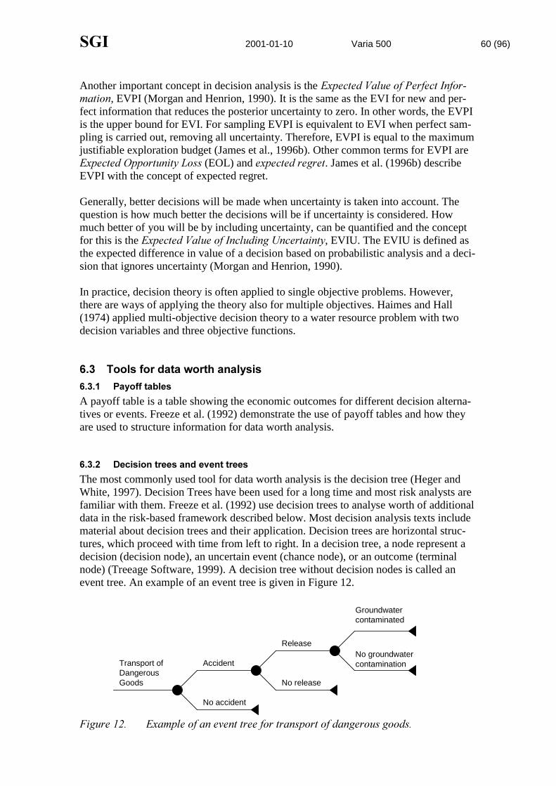
6*, 2001-01-10 Varia 500 60 (96)

Another important concept in decision analysis is the ([SHFWHG�9DOXH�RI�3HUIHFW�,QIRU�PDWLRQ, EVPI (Morgan and Henrion, 1990). It is the same as the EVI for new and per-fect information that reduces the posterior uncertainty to zero. In other words, the EVPIis the upper bound for EVI. For sampling EVPI is equivalent to EVI when perfect sam-pling is carried out, removing all uncertainty. Therefore, EVPI is equal to the maximumjustifiable exploration budget (James et al., 1996b). Other common terms for EVPI are([SHFWHG�2SSRUWXQLW\�/RVV (EOL) and H[SHFWHG�UHJUHW. James et al. (1996b) describeEVPI with the concept of expected regret.

Generally, better decisions will be made when uncertainty is taken into account. Thequestion is how much better the decisions will be if uncertainty is considered. Howmuch better of you will be by including uncertainty, can be quantified and the conceptfor this is the ([SHFWHG�9DOXH�RI�,QFOXGLQJ�8QFHUWDLQW\, EVIU. The EVIU is defined asthe expected difference in value of a decision based on probabilistic analysis and a deci-sion that ignores uncertainty (Morgan and Henrion, 1990).

In practice, decision theory is often applied to single objective problems. However,there are ways of applying the theory also for multiple objectives. Haimes and Hall(1974) applied multi-objective decision theory to a water resource problem with twodecision variables and three objective functions.

�� 7RROV�IRU�GDWD�ZRUWK�DQDO\VLV

�� 3D\RII�WDEOHV

A payoff table is a table showing the economic outcomes for different decision alterna-tives or events. Freeze et al. (1992) demonstrate the use of payoff tables and how theyare used to structure information for data worth analysis.

�� 'HFLVLRQ�WUHHV�DQG�HYHQW�WUHHV

The most commonly used tool for data worth analysis is the decision tree (Heger andWhite, 1997). Decision Trees have been used for a long time and most risk analysts arefamiliar with them. Freeze et al. (1992) use decision trees to analyse worth of additionaldata in the risk-based framework described below. Most decision analysis texts includematerial about decision trees and their application. Decision trees are horizontal struc-tures, which proceed with time from left to right. In a decision tree, a node represent adecision (decision node), an uncertain event (chance node), or an outcome (terminalnode) (Treeage Software, 1999). A decision tree without decision nodes is called anevent tree. An example of an event tree is given in Figure 12.

Transport ofDangerousGoods

Accident

No accident

Release

No release

Groundwatercontaminated

No groundwatercontamination

)LJXUH�� ([DPSOH�RI�DQ�HYHQW�WUHH�IRU�WUDQVSRUW�RI�GDQJHURXV�JRRGV�

6*, 2001-01-10 Varia 500 61 (96)

�� ,QIOXHQFH�GLDJUDPV

A tool with growing applications in decision analysis is the influence diagram, alsocalled relevance diagram. Heger and White (1997) argue that influence diagrams aremore effective than decision trees for data worth analysis. There are two main advan-tages of influence diagrams compared to decision trees:

1. The size of the influence diagram is a linear function of the number of variables,whereas the size of the decision tree is an exponential function.

2. Influence diagrams provide a better visual representation of the relationship amongvariables.

Another advantage is the ease of understanding for the decision-maker even for prob-lems with many variables, in contrast to decision trees that easily become difficult tounderstand. Other authors have also compared decision trees and influence diagrams,for example Call and Miller (Heger and White, 1997). They also describe the DecisionProgramming Language (DPL) as a tool that captures the useful features of both deci-sion trees and influence diagrams.

An influence diagram consists of chance nodes (ovals), decision nodes (rectangles),value nodes (diamonds), and sometimes deterministic nodes. Typical functions assignedto value nodes include cost-benefit-risk or simple cost functions (Heger and White,1997). The nodes of the influence diagram are inter-connected by arcs. Two types ofarcs exist; information arcs and conditional arcs. Together they show the flow of infor-mation and uncertainty through the decision-making process. Figure 13 shows an exam-ple of an influence diagram.

Treatment

DownstreamSampling

UpstreamSampling

WaterQuality

UpstreamData

DownstreamData

Violation ofStandard

Cost to theCity

)LJXUH�� ([DPSOH�RI�DQ�LQIOXHQFH�GLDJUDP�LOOXVWUDWLQJ�WKH�PRQLWRU�DQG�WUHDW�GHFL�VLRQ�SUREOHP��6DPSOLQJ�LV�SHUIRUPHG�XSVWUHDP�DQG�GRZQVWUHDP�RI�D�GLV�FKDUJH�SRLQW�LQ�D�ULYHU�WR�VWXG\�DUVHQLF�FRQFHQWUDWLRQV�UHJDUGLQJ�VDP�SOLQJ�RI�ULYHU�ZDWHU��DIWHU�+HJHU�DQG�:KLWH��

6*, 2001-01-10 Varia 500 62 (96)

Attoh-Okine (1998) explains the influence diagram tool for application on contaminatedland problems. Heger and White (1997) used an influence diagram to calculate theworth of historical data of water quality in a river (Figure 13). However, no calculationof the worth of additional, uncollected data was performed.

�� ([SHUW�V\VWHPV

Expert systems have only been used to a limited extent for data worth and decisionanalysis in problems related to contaminated land. The three main paradigms for expertsystems are; rule-based systems, neural networks, and Bayesian networks (Jensen,1998). A short presentation of these will be given based on Jensen (1998).

5XOH�EDVHG�V\VWHPV try to model the expert´s way of reasoning by means of a set ofrules. In rule-based systems the uncertainty is often treated by fuzzy logic (see section2.5.3), certainty factors etc.

A QHXUDO�QHWZRUN consists of one layer of input nodes, one layer of output nodes, andnormally 1-2 hidden layers. The network performs pattern recognition based on trainingresults from known input and output values. It is not possible to read the uncertainty inthe conclusion from a neural network. As an example, neural networks have been usedfor soil geology interpolation (Kumar et al., 2000) and estimation of hydrogeologicalparameters (Mukhopadhyay, 1999).

A %D\HVLDQ�QHWZRUN consists of nodes and arcs connecting the nodes. The arcs reflectcause-effect relationship and the strength of an effect is given as a probability. Bayesiannetworks can be updated when additional information becomes available. Other namesfor Bayesian networks are Bayes nets, belief networks, Bayesian belief networks(BBNs), causal probabilistic networks (CPNs), or causal networks. Similar to influencediagrams, they are useful in showing the structure of a decision problem. In fact, a Bay-esian network is equivalent to an influence diagram consisting of only chance nodes. Sofar, Bayesian networks have not been much applied to contaminated land problems.Software for Bayesian networks is presented in the appendix.

�� 6WUDWHJLHV�IRU�GDWD�ZRUWK�DQDO\VLV

�� 7UDGLWLRQDO�DSSURDFK��)L[HG�FRVW�RU�IL[HG�XQFHUWDLQW\

Two strategies have traditionally been used for sampling; (1) to minimise the samplingcost for a specified level of accuracy (usually variance), or (2) to minimise uncertaintyfor a given sampling budget. These are also the strategies that Gilbert (1987) and Hue-semann (1994) mention as the most commonly used in practice. In these strategies ad-ditional sampling have worth until uncertainty has been reduced to a specified level, oruntil there is no more money available for sampling. The first strategy often originatesfrom some kind of regulatory framework where the cost-efficiency is not the primarygoal.

Gilbert (1987) and Borgman et al. (1996a) provide cost functions that can be applied forboth strategies when the population mean should be determined. Cost functions are pre-sented for a number of sampling methods described below.

6*, 2001-01-10 Varia 500 63 (96)

6WUDWLILHG�UDQGRP�VDPSOLQJThe cost function presented is applicable when the main objective is to estimate theoverall population mean (all strata included), or population total (such as total amountof a contaminant). With the cost function the optimum number of samples in each stratacan be calculated. Equations for calculating the total number of samples are presentedfor (1) prespecified fixed cost, (2) prespecified variance, and (3) prespecified margin oferror (Gilbert, 1987). Both Gilbert (1987) and Borgman et al. (1996a) provide examplesof the calculations.

7ZR�VWDJH�VDPSOLQJIn two-stage sampling the target population is divided into primary units (first stage)and the primary units into sub-units (second stage). An example of two-stage samplingis when soil samples are divided into subsamples (aliquots) chosen for measurement.Gilbert (1987) provides a cost function and equations to calculate the optimal number ofsubsamples.

&RPSRVLWH�VDPSOLQJGilbert (1987) presents a cost function for composite sampling. The number of batches,composites in each batch, and subsamples from each composite has to be selected (abatch is a group of population units). The idea is to select values for the number ofbatches, composites and subsamples that will minimise the variance (or the cost if thevariance is prespecified).

Garner et al. (1996) present a number of models for cost-effective composite samplingusing the concept of relative cost factors. One of the models is a multivariate modelwhere more than one contaminant can be detected.

'RXEOH�VDPSOLQJDouble sampling can be used when two different techniques are available for measuringthe contaminant concentration. An example is when one field screening technique andone laboratory analysis method is used in combination. For a cost-efficient solution onlya small number of samples are analysed with both techniques but many samples areanalysed with the cheaper of the two methods (note that this cost-efficiency is differentfrom the cost-efficiency concept in a decision analysis framework). Gilbert (1987) pres-ents a cost function and some equations to determine the optimum number of samplesfor each of the two measurement techniques. He also presents a case study.

�� 0LVFODVVLILFDWLRQ�FRVW�DQG�ORVV�IXQFWLRQV

To classify and area as “contaminated” when it in reality is not, is a PLVFODVVLILFDWLRQ.The opposite situation is also a misclassification, i.e. a “clean” area is classified as“contaminated”. As described in section 5.4 these errors are generally called IDOVH�SRVL�WLYH (overestimation or overclassification) and IDOVH�QHJDWLYH (underestimation or under-classification) respectively. Each misclassification that is made leads to some kind ofcost. Aspie and Barnes (1990) present a simple cost function for the total cost of mis-classification (�F):

XXRRF$$ ⋅+⋅= $$$

6*, 2001-01-10 Varia 500 64 (96)

where �R and �X are the costs of overclassification and underclassification respectively(per unit area). $R and $X represent the total area that is overclassified and underclassi-fied respectively.

Myers (1997) presents a cost optimisation graph (Figure 14) for optimising the numberof samples to be taken. A large error in estimated concentration leads to a large misclas-sification cost. This often occurs when only few samples are taken, i.e. the samplingcost is low. When more samples are taken the sampling cost increases but the misclassi-fication cost decreases. The cost of false positive classification can quite precisely beestimated in terms of engineering cost (Myers, 1997). An investment in sampling willprobably reduce this cost. The optimum number of samples occurs where the total costis at a minimum, i.e. at the cost optimum. At the cost optimum, marginal cost equalsmarginal benefit.

The loss function in Figure 14 is a simple and symmetric one. It only considers falsepositive decision errors (overestimation). Flatman and Englund (1991) present thesymmetrical least-squares loss function, which incorporates both false positive and falsenegative classification errors. With this function the loss (cost) increases with the squareof the size of the error. Usually, asymmetric loss functions are more realistic than sym-metrical ones. Flatman and Englund (1991) as well as Myers (1997) present asymmetricloss functions that also incorporate false negative errors (underestimation). One is theVWHS�IXQFWLRQ. If there is a false positive decision there will be a fixed cost of remedia-tion and if there is a false negative error a fixed estimated cost due to health effects willappear.

)LJXUH�� $�FRVW�RSWLPLVDWLRQ�JUDSK�IRU�VDPSOLQJ��$IWHU�-�0�5HQGX�LQ�0\HUV��

An improvement of the step function is the 9�FXUYH�ORVV�IXQFWLRQ (Figure 15). In thisloss function the costs are not fixed, instead they increase when the decision error in-creases. The positive portion of the graph reflects false negative errors, bringing healtheffect costs. The negative part of the graph corresponds to remediation costs due to falsepositive errors. Myers (1997) also presents a K\EULG�VWHS�9�FXUYH, where the false posi-tive errors result in a fixed remediation cost, while the right hand side of the graph isidentical with Figure 15.

Misclassification Cost

Sampling Cost

Total Cost

Number of Samples

Err

or (

Cos

t)

OptimumCost

6*, 2001-01-10 Varia 500 65 (96)

)LJXUH�� 7KH�9�FXUYH�ORVV�IXQFWLRQ��(UURU�LV�GHILQHG�DV�WKH�GLIIHUHQFH�EHWZHHQ�WKHWUXH�FRQFHQWUDWLRQ�DQG�WKH�DFWLRQ�OHYHO��$/��IRU�DOO�LQFRUUHFW�GHFLVLRQV�7KH�H[SHFWHG�ORVV�LV�D�IXQFWLRQ�RI�FRQFHQWUDWLRQ��DIWHU�)ODWPDQ�DQG(QJOXQG��

Flatman and Englund (1991) argue that the loss function must be defined along withother goals and objectives before a sampling design is determined.

Thompson and Fearn (1996) present cost and loss functions similar to the ones above.The loss function expresses the expected loss (cost) as a function of uncertainty (vari-ance), and cost of sampling and analysis. It expresses how the loss to an end-user in-creases with the magnitude of the measurement error in some way (the error is definedas the difference between the estimated and the true concentration). The true concentra-tion is usually not known but the optimal division of resources between sampling andanalysis can still be found by minimising the loss function. For simple loss functionsminimisation can be made algebraically but this may not be possible for more compli-cated functions. Thompson and Fearn (1996) present solutions for some simple sym-metrical loss functions as the quadratic loss function, the V curve loss function, and anempirical asymmetrical step function. For practical use the cost function must be de-signed for the particular problem and for example penalty costs could be incorporated.

The described loss functions consider misclassification of the whole area and do notaddress local misclassification. A SUREDELOLW\�EDVHG�FRVW�IXQFWLRQ proposed by Aspieand Barnes (1990) manages this. It can be derived from the simple cost function pre-sented in the beginning of this section, based on concept of H[SHFWHG�FRVW�RI�HUURUV.Aspie and Barnes (1990) present an infill-sampling strategy for situations when a set ofsamples has been taken (known location and known value) and another sampling roundis planned. The optimal locations are determined out of a set of possible new samplelocations. The procedure is based on the H[SHFWHG�FRVW�RI�HUURUV criterion using simplekriging. The probabilities of a false positive or false negative can be obtained for eachpoint in a block model by using ordinary, simple, indicator, or probability kriging(Myers, 1997).

3AL 4AL-AL-2ALError axis

Cost

AL 2AL

e2 = y-AL

6*, 2001-01-10 Varia 500 66 (96)

�� 8QFHUWDLQW\�EDVHG�VWRSSLQJ�UXOHV

In this section a selection of sampling approaches with uncertainty-based stopping ruleswill be presented. These stopping rules do not take sampling cost, other costs or bene-fits, or the economical worth of data into account specifically. However, it appears thatthese approaches can be slightly modified to incorporate the aspects of cost and dataworth.

Johnson (1996) has demonstrated an DGDSWLYH�VDPSOLQJ strategy, i.e. the sampling isperformed in subsequent stages. It is based on the objective to minimise uncertaintyabout the extension of contamination and uses a Bayesian/geostatistical methodology.An initial conceptual model based on soft information is used when sampling begins.Hard and soft data are combined and updating is performed by indicator kriging. Newsample locations are selected from a set of potential sampling points based on the ob-jective of maximising the area classified as clean at the 80 % certainty level. Data worthare not considered in the approach but could probably be incorporated relatively easy.Johnson (1996) states that his method for handling uncertainty ³«OHDGV�QDWXUDOO\�WRPHDVXUHV�RI�EHQHILW�RQH�PLJKW�H[SHFW�IURP�DGGLWLRQDO�GDWD�FROOHFWLRQ´.

Chiueh et al. (1997) present a decision support system for probability analysis in soilcontamination. It is based on a database, a model with an indicator kriging algorithmand a Geographic Information System (GIS). The whole study site is divided intoblocks in a square grid. The user must specify a threshold level of contaminant concen-tration. Also, probabilistic criteria must be specified for when to remediate and when totake additional samples. These are based on the probability of exceeding the thresholdlevel, and the probability of a false positive or negative classification. If the criteria arenot fulfilled, additional sampling may have to be performed. The system has no costfunction integrated, so cost calculations have to be made by the user.

Robbat (1996) has developed a strategy for adaptive sampling based on the DQO proc-ess. Field analysis techniques are proposed for cost-effectiveness. Several samplingrounds are made until confidence in the conceptual model is obtained. An illustrativeflow chart of the process is presented. However, the stopping rule for sampling is ex-pressed rather vague: ³'RHV�TXDQWLWDWLYH�DQDO\VLV�YHULI\�VLWH�VFUHHQLQJ"´ It is proposedthat sampling should be directed by geostatistical techniques. Costs for different fieldanalysis techniques are presented in an appendix.

Stenback and Kjartanson (2000) present another geostatistical approach for adaptivesampling. Samples are located to regions where there is high uncertainty regarding if theconcentration exceeds a specified threshold level. Samples are spaced according to theUDQJH of a variogram calculated from sample data. A probability contour bounds thecontaminated area and the sample collection ceases when there is low probability for thearea outside the boundary to exceed the threshold. The probability map could be devel-oped by indicator kriging, ordinary kriging, or a less well-known third method(Stenback and Kjartanson, 2000).

�� %D\HVLDQ�GHFLVLRQ�DQDO\VLV

(DUO\�IUDPHZRUNVSeveral early frameworks for evaluation of data worth were reported during the 1970´s.Davis and Dvoranchik (1971) demonstrated a framework to determine the value of ad-

6*, 2001-01-10 Varia 500 67 (96)

ditional information about annual peak flow in a stream for a bridge construction prob-lem. They applied the concept of expected opportunity loss (EOL) to calculate the worthof data. Gates and Kisiel (1974) applied the EOL concept on a groundwater model. Er-ror in model prediction was coupled to a loss function and reduced by more informa-tion.

Maddock (1973) presented a management model for an irrigated farm with the purposeto maximise the expected profit of the farm. The analysis results in a decision on crop-ping and water pumping patterns over a design period, a choice of groundwater model,the ranking of data worth for different types of data, and the ranking of priority of fur-ther data collection. The concept of H[SHFWHG�UHJUHW is used to measure the profit lossdue to non-optimal parameter values in the model. Only direct monetary costs are con-sidered in the model, not cost of failure since no failure criterion is defined.

Grosser and Goodman (1985) used loss functions and Bayesian decision theory to de-termine the optimal sampling frequency for chloride in a public water supply well.Three different loss functions were used for different chloride concentrations. The opti-mum number of samples was based on calculations of expected loss.

Ben-Zvi et al. (1988) demonstrated how preposterior analysis in a risk-based Bayesianframework can be used as a tool to assess the value of data before they become avail-able. The methodology was applied to a problem of aquifer contamination. Three differ-ent states of contaminant intrusion into the aquifer were assumed to be possible andthree different courses of action (decisions) was considered. Since decisions taken underuncertainty may lead to losses, loss functions are discussed. They define risk as“H[SHFWHG�ORVV” or as “WKH�DYHUDJH�ORVV�RI�D�FRQVLVWHQW�GHFLVLRQ�PDNHU”. The value ofadditional information (data worth) is defined as the expected reduction in risk, which isequal to the difference between the prior risk and the preposterior risk. The preposteriorrisk is calculated as a weight average of the minimal posterior risks, where the weightsare the prior probabilities for the different states.

The value of hydrogeological information for risk-based remedial action decisions wasstudied by Reichard and Evans (1989). They defined the total social cost (76&L) of anaction DL as:

( )XLULL5H&&76& −+= 1

where&L = economic cost of remedial action�DL&U = cost per unit risk (assumed constant)HL = efficiency of action DL in reducing risk (0 ≤ HL ≤ 1)5X = uncontrolled risk level (5X ≥ 0)

The concept of expected opportunity loss (EOL) is used to calculate the value ofgroundwater monitoring. The computation is performed in a general three-step frame-work.

)UHH]H�HW�DO�The framework presented by Freeze et al. (1992; 1990) is a framework for decisionanalysis. It is based on an objective function Φ of the form (Freeze et al., 1990):

6*, 2001-01-10 Varia 500 68 (96)

( ) ( ) ( )[ ]W5W&W%L

7

W

−−+

=Φ ∑=0 1

1

where %�W� = the EHQHILWV in year W, &�W� = the FRVW in year W, and 5�7� = the ULVN in year W.All of these parameters are expressed in monetary terms. The optimal decision from arisk perspective is achieved when the objective function is maximised. At this optimumthe risk level is called optimal risk. The risk is defined as the SUREDELOLW\�RI�IDLOXUH mul-tiplied with the FRVW�RI�IDLOXUH. The IDLOXUH�FULWHULRQ has to be defined in the individualcase. Note that benefits, cost, and cost of failure, are all economic terms. All other in-formation, such as sample data, geological information, engineering considerations etc.,are combined into one single term: the probability of failure.

In this framework, an additional measurement has worth only if the risk reduction itprovides exceeds the cost of obtaining it. Each new sample or measurement brings anadditional cost to the site-investigation, but it also provides additional information sothat the probability of failure is reduced. The question is how much new information anadditional measurement provides in relation to the additional cost. Freeze et al. (1992)define data worth in a precise way as ³«WKH�LQFUHDVH�LQ�WKH�H[SHFWHG�YDOXH�RI�WKH�RE�MHFWLYH�IXQFWLRQ�EHWZHHQ�WKH�SULRU�DQDO\VLV�DQG�WKH�SUHSRVWHULRU�DQDO\VLV�GXH�WR�WKHDYDLODELOLW\�RI�WKH�SURSRVHG�DGGLWLRQDO�PHDVXUHPHQWV´. The prior and preposterioranalyses refer to the different stages of Bayesian updating (see section 2.4.2).

In the framework, data worth analysis is a tool for the rational design of a field investi-gation program. Its purpose is to reduce (1) the uncertainty about the natural system, (2)the cost of the site-investigation programme and (3) the associated risks. According toFreeze et al. (1992) data worth analysis can be used in two ways: (a) to compare alter-native data-collection programmes, or (b) to be used as a stopping rule to decide whenno further measurements should be made.

Freeze et al.(1992) applied the concept of data worth on a hypothetical hydrogeologicalproblem. Some of the methods they propose to determine the probability of failure in-cludes search theory, stochastic simulation, and indicator kriging. They also demon-strate the concept of UHJUHW. Regret is defined as the price that must be paid for selectingthe non-optimal alternative given perfect knowledge.

-DPHV�DQG�)UHH]HJames and Freeze (1993) developed a Bayesian decision framework for addressingquestions of hydrogeological data worth. The framework has much in common with theframeworks based on optimisation (see section 6.4.5) but uses an objective functionidentical to the one presented by Freeze et al. (1990). An indicator simulation algorithmincorporates hard and soft data regarding the continuity of an aquitard. In a preposterioranalysis the H[SHFWHG�YDOXH�RI�VDPSOH�LQIRUPDWLRQ (EVSI) and the H[SHFWHG�YDOXH�RISHUIHFW�LQIRUPDWLRQ (EVPI) is evaluated. James and Freeze (1993) suggest that the bestsample location is not necessary the point of greatest uncertainty. The best sample loca-tion may also depend on both uncertainty and on the decision being made.

'DNLQV�HW�DO�Dakins et al. (1994) presented a decision framework for remediation of PCB-contaminated sediments. Instead of a fixed failure cost they use a loss function, where

6*, 2001-01-10 Varia 500 69 (96)

the loss (cost) is a function of the difference between the true contaminated area and theremediated area. Their analysis includes the H[SHFWHG�YDOXH�RI�LQFOXGLQJ�XQFHUWDLQW\(EVIU) and EVPI. In a later paper Dakins et al. (1995) extended their analysis to in-clude EVSI. They utilised Bayesian Monte Carlo methods to calculated EVSI in a pre-posterior analysis. A conclusion was that the calculated EVSI should be regarded as anupper bound due to a number of simplifying assumptions in the analysis.

-DPHV�DQG�*RUHOLFNJames and Gorelick (1994) presented a Bayesian data worth framework for aquifer re-mediation programs. Bayesian decision analysis is used to handle contaminant transportin a spatially heterogeneous environment. The framework consists of three modules: (1)A module with numerical modelling and 0RQWH�&DUOR�VLPXODWLRQ to predict the probablelocation of the contaminant plume, (2) a module for estimation of remediation costbased on FDSWXUH�]RQH�WKHRU\, and (3) a geostatistical module with LQGLFDWRU�NULJLQJ tocombine prior information with sample information. The framework evaluates themonetary worth of spatially correlated samples (at observation wells) when delineatinga contaminant plume. Measurements are made one by one in a stepwise manner and theoptimal number of measurements is estimated, as well as the best location for the nextsample. Prior, preposterior and posterior analyses are performed (Figure 16). Collectionof data ceases when the cost of acquisition is greater that the reduction in remediationcost the next measurement would bring. The evaluation of data worth is performedduring the preposterior analysis.

)LJXUH�� 2XWOLQH�RI�WKH�VWHSV�LQ�WKH�GDWD�ZRUWK�IUDPHZRUN�XVLQJ�SULRU��SUHSRVWH�ULRU��DQG�SRVWHULRU�DQDO\VHV��DIWHU�-DPHV�DQG�*RUHOLFN��

3ULRU�$QDO\VLVEstimate remediation costusing known information

3UHSRVWHULRU�$QDO\VLVFind best location for new sample where

expected sample worth is a maximum

Is sample likely to becost-effective?

Collect sample

3RVWHULRU�$QDO\VLVUpdate estimate of remediation

cost using new sample information

Yes

NoStop

6*, 2001-01-10 Varia 500 70 (96)

An interesting conclusion made by�James and Gorelick (1994) is that even if the worthof a single sample is less than its unit cost (which would indicate that the sample shouldnot be taken), it may still be worthwhile to collect it. The information in the single sam-ple may not be enough but combined with additional samples it may still be cost-effective to collect the sample.

-DPHV�HW�DO�James et al. (1996a; 1996b) present risk-based decision analysis frameworks for reme-diation decisions of contaminated soil and groundwater. These are stripped-down ap-proaches of the framework presented by Freeze et al. (1992; 1990). They illustrate howEVPI can be calculated based on the concept of expected regret. The quality of a sam-pling program is described by the VDPSOH�UHOLDELOLW\. The reliability ranges from 0 formeasurements of no value to 1 for perfect sampling. The sample worth is calculated bya simplified data worth equation (assuming no false detections of failure):

6DPSOH�ZRUWK� �6DPSOH�UHOLDELOLW\�î�(93,

It is pointed out that there will be significant uncertainty in the calculated sample worthbut that good estimates of the cost-effectiveness of a sampling program still can bemade.

%8'$Abbaspour et al. (1996) present a data worth model under the acronym BUDA, Baye-sian Uncertainty Development Algorithm. The purpose of the data worth model is toanalyse alternative sampling schemes in projects where decisions are made under un-certainty. The procedure in BUDA begins with problem definition, conceptualisation,definition of a goal function, definition of spaces etc. Four different problem spaces areidentified: (1) the space of alternative decisions, (2) the space of states of nature, (3) thespace of potential experiments to be performed, and (4) the space of samples (numberand location). Uncertainty is divided into natural and informational uncertainty. Propa-gation of uncertainty is performed by Latin Hypercube and Monte Carlo methods. Thefailure criterion must be defined individually for each project. The EVSI is evaluated foreach sampling scheme. In addition to EVSI, “the highest return value” of additionalsamples is analysed, i.e. the number of samples that maximises the return is identified.This number of samples should be collected in the first sample round. The data worthmodel has been applied to a landfill leachate plume (Abbaspour et al., 1998).

6PDUW�6DPSOLQJThe Smart Sampling approach is based on the risk-based decision framework presentedby Freeze et al. (1990). The basis is an economic objective function (Kaplan, 1998):

7RWDO�&RVW� �&KDUDFWHULVDWLRQ�&RVW��7UHDWPHQW�&RVW��)DLOXUH�&RVW

In principle, this function is identical to the objective function presented by Freeze et al.(1990). The expected failure cost is the probability of failure multiplied by the cost offailure. The Smart Sampling approach requires explicit decision rules, such as whetheror not a piece of ground is contaminated or uncontaminated. In this example the failuresare identical to the type I and type II errors described in section 5.4:

6*, 2001-01-10 Varia 500 71 (96)

Type I error: Removal of uncontaminated soil, if not required.Type II error: Failure to remove contaminated soil, if required.

Both types of failures involve a cost that is taken into account by the objective function.

The Smart Sampling process is designed to be iterative. This means that samples aretaken few at a time, the information is analysed, the objective function updated, and adecision to take more samples is based on predictions of the worth of additional samplestowards minimising the total cost of the remediation (Kaplan, 1998). Since spatial cor-relation of contaminant concentrations usually exists between sample locations at a site(Flatman and Yfantis, 1996), geostatistics is used as a tool. The distribution of contami-nant concentrations is studied in a histogram and the spatial correlations in a variogram.Before additional samples are taken a SUHSRVWHULRU�DQDO\VLV is performed. This is carriedout by geostatistical simulation, typically kriging. The purpose of the simulation is tocalculate how much the probability of failure will decrease when the additional infor-mation from sampling will be supplied. Since the probability of failure will change, sowill the value of the objective function. This makes it possible to calculate the worth ofadditional sampling before it has been undertaken. When additional sampling has beenperformed a new analysis will be carried out. This iterative procedure continues untiladditional samples will no longer reduce the objective function.

The Smart Sampling approach, as presented by Kaplan (1998), develops graphical rep-resentations for decision makers, site owners, and the general public so that they maybetter understand the costs and consequences of achieving varying levels of cleanup at acontaminated site. Smart Sampling is developed at Sandia National Laboratories inUSA. The purpose is to automate the decision framework into a user-friendly softwaretool.

A bibliography of projects where the Smart Sampling approach has been used is avail-able at the internet link http://www.nwer.sandia.gov/sample/bibliography.html.

5XVVHOO�DQG�5DELGHDXRussell and Rabideau (2000) evaluated the uncertainty in a risk-based decision analysisframework for Pump-and-Treat design. In total, 27 different remediation design alterna-tives were studied and for each alternative 36 calculations of the net present value (theobjective function) were made, with the following variations in the framework:

� Two degrees of aquifer heterogeneity� Two definitions of system failure� Three definitions of cleanup standard� Three failure costs

Based on these calculations, decision histograms were created, showing how manytimes each design alternative was favourable. It was found that the failure cost was themost important source of uncertainty in the analysis. Also, the need of a clear definitionof failure was identified.

6*, 2001-01-10 Varia 500 72 (96)

�� 2SWLPLVDWLRQ�DSSURDFKHV

The goal of frameworks based on optimisation has often been to minimise samplingcosts while estimating some quantity (James and Gorelick, 1994). Here, a few worksbased on optimisation approaches will be described in short.

Tucciarelli and Pinder (1991) presented an optimal data acquisition strategy forgroundwater remediation. The algorithm finds the total minimum for measurement costand pumping cost. They use a deterministic simulation model but a stochastic optimisa-tion approach. It was found that the optimisation algorithm was computationally inten-sive.

Wagner et al. (1992) used a stochastic optimisation model with the purpose to minimisetotal cost of installation and operation of pumping wells for containment of a contami-nated groundwater plume. The value of information about hydraulic conductivity is cal-culated for different cases. It depends on when in the decision-making process the in-formation is obtained and to what extent this information can affect further decisions.

Wagner (1999) presents a methodology for evaluation of data worth for groundwatermanagement. The methodology consists of four steps: (1) The optimal groundwatermanagement strategy is determined by a PDQDJHPHQW�PRGHO. The goal is to identify theleast-cost remediation strategy (optimal pumping rates) that ensures water quality stan-dards are met at a specified reliability level. This is performed by QRQ�OLQHDU�PD[LPXPOLNHOLKRRG�HVWLPDWLRQ�WKHRU\. (2) A monitoring�QHWZRUN�GHVLJQ�PRGHO is used to identifythe sampling strategy that will minimise uncertainty in model predictions for a specifieddata collection budget. The network design model is formulated as an LQWHJHU�SURJUDPPLQJ�RSWLPLVDWLRQ problem. (3) The management model is resolved based onthe updated model prediction uncertainty from the network design model. The purposeis to determine the reduction in management cost if the optimal sampling strategy wasimplemented. (4) The worth of the sampling strategy is determined by comparing thereduction in management cost (worth of sample information) with the cost of data col-lection. The strategy is justified only if the worth of sample information exceeds sam-pling cost. Steps 2-4 can be repeated for a series of data collection budgets to identifythe least-cost alternative.

Freeze and Gorelick (1999) compare the two approaches decision analysis and stochas-tic optimisation for aquifer remediation. A conclusion is that both strategies are wellsuited to assess the worth of additional data. A literature review is provided of researchin optimisation and decision analysis for aquifer restoration. It was found that dataworth within an optimisation framework has only been addressed in a few papers.

�� 5XOH�EDVHG�DGDSWLYH�VDPSOLQJ

An interesting but very different approach to sampling is the adaptive sampling�ap-proach as described by Cox (1999). It does not require any specific statistical model forthe spatial distribution of contaminants, but instead constructs an increasingly accuratenon-parametric approximation to it as sampling proceeds (Cox, 1999). In other words,the system “learns” from data as sampling goes on. 'HFLVLRQ�UXOHV must first be devel-oped and a vector of decision parameters describes them. The decision rules are createdfor the specific problem at hand, but are typically rules that promote cost-effective sam-pling and cleanup. When the decision parameters have been determined the adaptive

6*, 2001-01-10 Varia 500 73 (96)

sampling strategy can be optimised by VLPXODWLRQ�RSWLPLVDWLRQ for identifying approxi-mately optimal adaptive sampling decision rules. The simulation is performed usingexisting sample data. In the simulation, different combinations of values for the decisionparameters are used and the combinations of parameter values that meet the perform-ance criteria best are considered optimal.

Cox (1999) provides the following example of the adaptive sampling approach appliedto contaminated land. Four decision parameters are used:

N = initial number of random samples to be taken from the area of concern. These sam-ples are in addition to already collected samples.

S = number of soil samples to take from each newly sampled property (the area of con-cern is divided into a number of properties; in the example, each property is eitherto be remediated in its entirety or not at all).

K = maximum allowed length of a “search list”. This is a list of properties with thehighest average sample concentration seen so far.

T = action threshold. A property is to be remediated if, and only if, the mean concentra-tion of its S sample values exceeds T.

The decision parameter vector (N, S, K, T) is used in the simulation-optimisation to findthe optimal combination of values. Then, the procedure of the adaptive sampling fol-lows (a property is called IDWKRPHG when S samples have been taken from it and fromeach of its immediate neighbours):

1. Randomly sample N previously unsampled locations in the area of concern.2. Place the K properties with the highest mean concentrations so far on the search list.3. Fathom each property on the search list by taking S samples at the property and its

neighbours, and remove the property from the list when it has been fathomed.4. Whenever a property is found with a mean concentration greater than the values for

properties not included on the initial search list (step 2), place that property on thesearch list.

5. Continue steps 3 and 4 until the search list is empty, i.e. until both the initial proper-ties on the list and the ones added later has been removed. This terminates the adap-tive sampling phase.

6. Remediate those properties with a mean concentration exceeding T.

Cox (1999) calls this procedure ZRUVW�ILUVW�DGDSWLYH�VHDUFK, in that the search concen-trates on properties with high soil contamination levels. He also presents a strategy forthe simulation-optimisation of the decision parameter vector.

The technique of adaptive sampling provides a practical approach to decide where tosample next, when to stop, and what to do to optimise an overall performance objective(Cox, 1999). The performance objective can be of different types, such as to minimisethe number of misclassification errors, or expected utility. It can also be applied withrisk-cost-benefit criteria.

One drawback in the example presented above is that the sampling may require manyvisits to the area of concern due to the multi-stage nature of adaptive sampling. How-ever, it is possible to use only a few stages (e.g. a two stage sampling procedure) if theset of decision parameters is modified.

6*, 2001-01-10 Varia 500 74 (96)

Note that the term adaptive sampling can be used for sampling approaches that are verydifferent from the one presented here, e.g. those described in section 6.4.3.

�� 6DPSOLQJ�IRU�PRGHO�GLVFULPLQDWLRQ

Another different approach to the worth of sample information is presented by Knop-man and Voss (1988). The purpose of their study was to develop a methodology forchoosing between different contaminant transport models based on errors in model pre-dictions. They presented a methodology to compare different sampling designs in theirefficiency of acquiring information for discrimination among models. Better samplingdesigns maximise the difference in predictions between models. The model predictionsare compared by a defined objective function (a sum of squares objective function). Theobjective function is calculated for each sampling design. A sampling design with alarger value of the objective function supplies more information than a design with asmaller objective function value.

6*, 2001-01-10 Varia 500 75 (96)

�� ',6&866,21

�� *HQHUDO

This literature review covers several topics related to sampling. As shown, the literatureon the subject is quite extensive and covers much more than is presented in this report.There is a number of aspects about the material that is worth some comments. In thischapter a discussion is given with the purpose to identify research needs and areas of thesampling problem that could be developed further.

�� 3ULRU�LQIRUPDWLRQ�DQG�H[SHUW�NQRZOHGJH

Many of the techniques and methodologies for sampling strategies are based on the as-sumption that no prior information about a site is available. Examples of such methodsinclude classical sampling statistics, search theory etc. Some work has been done toinclude prior information like site history, geological conditions etc. in a quantitativeanalysis but in practice prior information is often included only in a qualitative way.More and better methods to include prior information quantitatively are needed. This isfundamental because prior information can be as important as the sampling information.

�� 0RGHOV

The amount of data needed to understand the behaviour of a physical system may ex-ceed the amount of data needed to make a good decision (Maddock, 1973). The physicalmodel that uses the data may be far more complex than can be handled by the decisionprocess. This may lead to collection of excessive data and overly sophisticated models(Maddock, 1973). Some of the models that have been encountered in this literature re-view have been quite complex, while some have been fairly simple. In many cases asimple model will supply sufficient information at a low cost. In other situations moreadvanced models will be needed. A conclusion is that there is a need for a methodologyhow to select a model of optimal complexity level. The methodology should be risk-based, taking the model uncertainty and the cost of application into account.

�� 3DUWLFXODWH�VDPSOLQJ�WKHRU\

The presentation of the particulate sampling theory is described relatively detailed inthis report compared to other topics presented. The reason is that the sampling theory isrelatively unknown among practitioners, at least in Sweden. As mentioned previously,the theory was developed to promote mineral extraction but has also been applied toenvironmental problems. However, it is not evident that all aspects of the theory areapplicable in all situations. For example, in the theory the SDUWLFOH�PDVV is importantbecause it relates to the grade in mineral exploration. In some contamination problems itmay instead be the VXUIDFH�DUHD of particles that is of primary concern, since the con-taminant may cover the particle surface, not the particle volume. Probably, some aspectsof the theory could be modified to include such aspects for environmental problems.

6*, 2001-01-10 Varia 500 76 (96)

�� 6DPSOLQJ�HUURUV

Several of the different types of sampling errors presented in this report can be difficultto quantify. Practical experience of the size of each error can rarely be found in the lit-erature. Information on how to quantify these errors is appreciated. As an example, thevariability of contaminant concentrations in soil around a sampling point (short range),has only been addressed in a small number of papers but the conclusions have been thatthis type of uncertainty can be very large. However, these conclusions are only valid forthese specific studies. The short-range variability will most likely depend on the sitehistory, the geology, and the type of contaminant present. In situations where the vari-ability is large, a single sample may randomly indicate “small contamination” or “largecontamination”. In this case, there will be a potential for making wrong decisions if thistype of sampling error is not taken into account. Another example of sampling error isthe bias that can be introduced by the sampling equipment. Generally, a methodology tohandle systematic sampling errors would be appreciated.

�� 6DPSOLQJ�VWUDWHJLHV

The question on how many samples to collect is always encountered in practice. Oneanswer is to use data worth analysis as discussed below. Today, other methods are beingused based on limited economic budgets or a desired accuracy of estimated properties.The literature on this matter is often restricted to certain types of problems, often sam-pling to estimate mean concentrations. Normally distributed data without any spatialcorrelation is often assumed. There is definitely a need for a review article or a publica-tion on how to determine the necessary number of samples in a structured way underdifferent assumptions, taking for example different sampling objectives, non-normallydistributed data, spatial correlation, prior knowledge, and sampling with multiple objec-tives into account. No such well-structured presentation has been found in the literature.The perfect guide to sampling is yet to be published.

A common misunderstanding regarding the systematic sampling pattern requires acomment. The misunderstanding can be found among consultants and in rare cases evenin the literature. Contrary to what many believe, sampling according to a systematic griddoes not imply that randomness therefore is missing and that statistical or geostatisticaltechniques cannot be used. As long as all sampling locations have the same probabilityof selection (as is the case for systematic sampling if the first sampling point is selectedrandomly) the sampling can be regarded as random. Therefore, samples collected ac-cording to a systematic sampling pattern can very well be analysed statistically or withgeostatistical techniques (provided that the grid itself is laid out randomly).

�� 'DWD�ZRUWK

The literature review has shown that data worth approaches have been used infrequentlyfor three decades. There are probably a number of reasons why the concept has not beenapplied to real world problems more often. One reason is that the concept is relativelyunknown. Another is that some methods are very computational intensive. The mainreason is however that much of the previous work on data worth analysis has been quitecomplicated and difficult to grasp for an average consultant or researcher working in thefield of contaminated land. This is especially true for the combination of data worthanalysis and optimisation techniques. The complexity has restricted the practical use of

6*, 2001-01-10 Varia 500 77 (96)

the data worth approach although the potential for its application is huge. Data worthanalysis could for example be applied not only contamination problems, but also toclassical geotechnical problems.

An exception to the complex papers discussed above is the work by James et al. (1996b)who present a stripped-down approach to data worth analysis. For broad picture analysisthis kind of approach could be sufficient, for example to determine whether a samplingprogram is cost-effective or not. The methodology could be developed further to handlecommon problems encountered in contamination problems in an effective but under-standable way. For in-depth analysis more sophisticated methods will probably beneeded. Here, the Bayesian-Markov chain analysis is such a method that could be ap-plied to data worth analysis of contaminated land on a relatively detailed level. Ofcourse, more traditional geostatistic tools can also be applied, such as kriging tech-niques.

Preferable, a range of methods of different complexity should be available for dataworth analysis. This will make it possible to select a simple approach when needed, forexample in early stages of a project. If such an analysis turns out to be insufficient, morecomplex methodologies could be applied.

In cases when data worth analysis has been applied to sampling problems, the samplinguncertainties have often been neglected. Some of the uncertainties may have been con-sidered, such as natural variability, while others have been ignored. If a practical dataworth methodology is developed, it must be able to handle the different types of uncer-tainty that evolve in a site-investigation.

In the risk-based decision analysis approach a cost arises when failure occurs, i.e. whenthe failure criterion is met. The importance of the choice of failure criterion needs to beevaluated. How will the result of the analysis change if a different failure criterion isused? Also, the criterion for when to start remediation must be chosen properly (this isidentical or closely related to the failure criterion). To begin remediation if the meanconcentration exceeds an action level may not be an appropriate approach in all situa-tions. The choice to start remediation must also be coupled to the different exposureroutes for humans and how the contaminants affect the environment. A basis for thechoice of failure and remediation criterion should be the source-path-target concept.Therefore, the data worth analysis will also have connections with the risk assessmentmethodology.

6*, 2001-01-10 Varia 500 78 (96)

5()(5(1&(6

Abbaspour, K.C., Schulin, R., Schläppi, E. and Flühler, H., 1996. A Bayesian approachfor incorporating uncertainty and data worth in environmental projects. Envi-ronmental Modeling and Assessment, 1996(1): 151-158.

Abbaspour, K.C., Schulin, R., van Genuchten, M.T. and Schläppi, E., 1998. Proceduresfor Uncertainty Analyses Applied to a Landfill Leachate Plume. Ground Water,36(6): 874-883.

Albert, R. and Horwitz, W., 1996. Coping with Sampling Variability in Biota: Percen-tiles and Other Strategies. In: L.H. Keith (Editor), Principles of EnvironmentalSampling. American Chemical Society, Washington, DC, pp. 653-669.

Alén, C., 1998. On Probability in Geotechnics. Random Calculation Models Exempli-fied on Slope Stability Analysis and Ground-Superstructure Interaction, Volume1. Dissertation Thesis, Chalmers University of Technology, Göteborg, 242 pp.

Aspie, D. and Barnes, R.J., 1990. Infill-Sampling Design and the Cost of ClassificationErrors. Mathematical Geology, 22(8): 915-932.

ASTM, 1995. Standard Guide for Developing Conceptual Site Models for Contami-nated Sites, ASTM Standards on Environmental Sampling. American Society forTesting and Materials, pp. E 1689-95, 1-8.

Attoh-Okine, N.O., 1998. Potential Application of Influence Diagram as a Risk As-sessment Tool in Brownfields Sites. In: K.B. Hoddinott (Editor), Superfund RiskAssessment in Soil Contamination Studies: Third Volume, ASTM STP 1338.American Society for Testing and Materials, West Conshohocken, pp. 148-159.

Ball, R.O. and Hahn, M.W., 1998. The Statistics of Small Data Sets. In: K.B. Hoddinott(Editor), Superfund Risk Assessment in Soil Contamination Studies: Third Vol-ume, ASTM STP 1338. American Society for Testing and Materials, West Con-shohocken, pp. 23-36.

Barcelona, M.J., 1996. Overview of the Sampling Process. In: L.H. Keith (Editor), Prin-ciples of Environmental Sampling. American Chemical Society, Washington,DC, pp. 41-61.

Barnard, T.E., 1996. Extending the Concept of Data Quality Objectives To Account forTotal Sample Variance. In: L.H. Keith (Editor), Principles of EnvironmentalSampling. American Chemical Society, Washington, DC, pp. 169-184.

Bear, J., 1979. Hydraulics of Groundwater. McGraw-Hill, New York, 569 pp.

Bear, J., 1988. Dynamics of Fluids in Porous Media. Dover Publications, New York,764 pp.

6*, 2001-01-10 Varia 500 79 (96)

Ben-Zvi, M., Berkowitz, B. and Kesler, S., 1988. Pre-Posterior Analysis as a Tool forData Evaluation: Application to Aquifer Conatmination. Water Resources Man-agement, 1988(2): 11-20.

Black, S.C., 1996. Defining Control Site and Blank Sample Needs. In: L.H. Keith(Editor), Principles of Environmental Sampling. American Chemical Society,Washington, DC, pp. 139-154.

Borgman, L.E., Gerow, K. and Flatman, G.T., 1996a. Cost-Effective Sampling for Spa-tially Distributed Phenomena. In: L.H. Keith (Editor), Principles of Environ-mental Sampling. American Chemical Society, Washington, DC, pp. 753-778.

Borgman, L.E., Kern, J.W., Anderson-Sprecher, R. and Flatman, G.T., 1996b. TheSampling Theory of Pierre Gy: Comparisons, Implementation, and Applicationsfor Environmental Sampling. In: L.H. Keith (Editor), Principles of Environ-mental Sampling. American Chemical Society, Washington, DC, pp. 203-221.

Bosman, R., 1993. Sampling Strategies and the Role of Geostatistics in the Investiga-tion of Soil Contamination. In: F. Arendt, G.J. Annokkée, R. Bosman and W.J.van den Brink (Editors), Contaminated Soil ´93, Fourth International KfK/TNOConference on Contaminated Soil. Kluwer Academic Publishers, Berlin, pp.587-597.

Box, G.E.P., Hunter, W.G. and Hunter, J.S., 1978. Statistics for Experimenters. An In-troduction to Design, Data Analysis and Model Buildning. John Wiley & Sons,New York, 653 pp.

Chai, E.Y., 1996. A Systematic Approach to Representative Sampling in the Environ-ment. In: J.H. Morgan (Editor), Sampling Environmental Media. American So-ciety for Testing and Materials, ASTM, West Conchohocken, pp. 33-44.

Chang, Y.H., Scrimshaw, M.D., Emmerson, R.H.C. and Lester, J.N., 1998. Geostatisti-cal analysis of sampling uncertainty at the Tollesbury Managed Retreat site inBlackwater Estuary, Essex, UK: Kriging and cokriging approach to minimisesampling density. The Science of the Total Environment, 1998(221): 43-57.

Chiueh, P.-T., Lo, S.-L. and Lee, C.-D., 1997. Prototype SDSS for Using ProbabilityAnalysis in Soil Contamination. Journal of Environmental Engineer, 123(5):514-520.

Christian, J.T., Ladd, C.C. and Baecher, G.B., 1994. Reliability Applied to Slope Sta-bility Analysis. ASCE, Journal of Geotechnical Engineering, 120(12): 2180-2207.

Clark, M.J.R., Laidlaw, M.C.A., Ryneveld, S.C. and Ward, M.I., 1996. EstimatingSampling Variance and Local Environmental Heterogeneity for both Known andEstimated Analytical Variance. Chemosphere, 32(6): 1133-1151.

Cox, L.A., 1999. Adaptive Spatial Sampling of Contaminated Soil. Risk Analysis,19(6): 1059-1069.

6*, 2001-01-10 Varia 500 80 (96)

Crépin, J. and Johnson, R.L., 1993. Soil Sampling for Environmental Assessment. In:M.R. Carter (Editor), Soil Sampling and Methods of Analysis. Canadian Societyof Soil Science/Lewish Publishers, pp. 5-18.

Cressie, N.A.C., 1993. Statistics for Spatial Data. John Wiley & Sons, New York, 900pp.

Dagdelen, K. and Turner, A.K., 1996. Importance of stationarity for geostatistical as-sessment of environmental contamination. In: S. Rouhani, R.M. Srivastava, A.J.Desbarats, M.V. Cromer and A.I. Johnson (Editors), Geostatistics for Environ-mental and Geotechnical Applications. ASTM, West Conshohocken, PA, pp.117-132.

Dakins, M.E., Toll, J.E. and Small, M.J., 1994. Risk-Based Environmental Remedia-tion: Decision Framework an Role of Uncertainty. Environmental Toxicologyand Chemistry, 13(12): 1907-1915.

Dakins, M.E., Toll, J.E., Small, M.J. and Brand, K.P., 1995. Risk-Based EnvironmentalRemediation: Bayesian Monte Carlo Analysis and the Expected Value of Sam-ple Information. Risk Analysis, 16(1): 67-79.

Davis, D.R. and Dvoranchik, W.M., 1971. Evaluation of the Worth of Additional Data.Water Resources Bulletin, 7(4): 700-707.

Decisioneering, 1996. Crystal Ball version 4.0, users manual, Denver.

Deutsch, C.V. and Journel, A.G., 1998. GSLIB, Geostatistcal Software Library andUser´s Guide. Oxford University Press, New York, 369 pp.

Drew, L.J., 1979. Pattern Drilling Exploration: Optimum Pattern Types and HoleSpacings When Searching for Elliptical Shaped Targets. Mathematical Geology,11(2): 223-254.

Englund, E.J. and Sparks, A.R., 1991. GEO-EAS 1.2.1 Geostatistical EnvironmentalAssessment Software User´s Guide. EPA 600/4-88/033, U.S. EnvironmentalProtection Agency, Las Vegas.

Fabrizio, M.C., Frank, A.M. and Savino, J.F., 1995. Procedures for Formation of Com-posite Samples from Segmented Populations. Environmental Science & Tech-nology, 29(5): 1137-1144.

Ferguson, C.C., 1992. The Statistical Basis for Sampling of Contaminated Land.Ground Engineering(June 1992): 34-38.

Ferguson, C.C., 1993. Sampling Strategy Guidelines for Contaminated Land. In: F.Arendt, G.J. Annokkée, R. Bosman and W.J. van den Brink (Editors), Contami-nated Soil ´93, Fourth International KfK/TNO Conference on ContaminatedSoil. Kluwer Academic Publishers, Bering, pp. 599-608.

6*, 2001-01-10 Varia 500 81 (96)

Ferguson, C.C. and Abbachi, A., 1993. Incorporating Expert Judgement into StatisticalSampling Designs for Contaminated Sites. Land Contamination and Reclama-tion, 1: 135-142.

Flatman, G.T. and Englund, E.J., 1991. Asymmetric loss functions for Superfund reme-diation decisions, Proceedings of the Business and Economic Statistics Sectionof the American Statistical Association, pp. 204-209.

Flatman, G.T. and Yfantis, A.A., 1996. Geostatistical Sampling Designs for HazardousWaste Sites. In: L.H. Keith (Editor), Principles for Environmental Sampling.American Chemical Society, Washington, DC, pp. 779-801.

Freeze, R.A., Bruce, J., Massman, J., Sperling, T. and Smith, L., 1992. HydrogeologicalDecision Analysis: 4. The Concept of Data Worth and Its Use in the Develop-ment of Site Investigation Startegies. Ground Water, 30(4): 574-588.

Freeze, R.A. and Cherry, J.A., 1979. Groundwater. Prentice-Hall, Englewood Cliffs,604 pp.

Freeze, R.A. and Gorelick, S.M., 1999. Convergence of Stochastic Optimization andDecision Analysis in the Engineering Design of Aquifer Remediation. GroundWater, 37(6): 934-954.

Freeze, R.A., Massman, J., Smith, L., Sperling, T. and James, B., 1990. Hydrogeologi-cal Decision Analysis: 1. A Framework. Ground Water, 28(5): 738-766.

Garner, F.C., Stapanian, M.A. and Williams, L.R., 1996. Composite Sampling for Envi-ronmental Monitoring. In: L.H. Keith (Editor), Principles of EnvironmentalSampling. American Chemical Society, Washington, DC, pp. 680-689.

Gates, J.S. and Kisiel, C.C., 1974. Worth of Additional Data to a Digital ComputerModel of a Groundwater Basin. Water Resources Research, 10(5): 1031-1038.

Gilbert, R.O., 1987. Statistical Methods for Environmental Pollution Monitoring. VanNostrand Reinhold, New York, 320 pp.

Goovaerts, P., 1997. Geostatistics for Natural Resources Evaluation. Applied Geostatis-tics Series. Oxford University Press, New York, 483 pp.

Gorelick, S.M., Freeze, R.A., Donohue, D. and Keely, J.F., 1993. Groundwater Con-tamination, Optimal Capture and Containment. Lewis Publishers, Boca Raton,385 pp.

Grosser, P.W. and Goodman, A.S., 1985. Determination of groundwater samplingfrquencies through Bayesian decision theory. Civ. Engng Syst., 2(December):186-194.

6*, 2001-01-10 Varia 500 82 (96)

Gustafson, G. and Olsson, O., 1993. The development of Conceptual Models For Re-pository Site Assessment, The Role of Conceptual Models in Demonstarting Re-pository Post-Closure Safety: Proceedings of an NEA Workshop. Nuclear En-ergy Agency, Organisation for Economic Co-operation and Development, Paris,pp. 145-158.

Guyonnet, D., Côme, B., Perrochet, P. and Parriaux, A., 1999. Comparing Two Meth-ods for Addressing Uncertainty in Risk Assessment. Journal of EnvironmentalEngineer, 1999(July): 660-666.

Haimes, Y.Y. and Hall, W., 1974. Multiobjectives in Water Resource Systems Analy-sis: The Surrogate Worth Trade Off Method. Water Resources Research, 10(4):615-624.

Halim, I.S. and Tang, W.H., 1993. Site Exploration Strategy for Geological AnomalyCharacterization. ASCE, Journal of Geotechnical Engineering, 119(2): 195-213.

Hammitt, J.K., 1995. Can More Information Increase Uncertainty? Chance, 8(3): 15-17,36.

Hammitt, J.K. and Shlyakhter, A.I., 1999. The Expected Value of Information and theProbability of Surprise. Risk Analysis, 19(1): 135-152.

Harr, M.E., 1987. Reliability-Based Design in Civil Engineering. Dover Publications,New York, 291 pp.

Heger, A.S. and White, J.E., 1997. Using influence diagrams for data worth analysis.Reliability Engineering ans System Safety, 1997(55): 195-202.

Hoffman, F.O. and Hammonds, J.S., 1994. Propagation of Uncertainty in Risk Assess-ments: The Need to Distinguish Between Uncertainty Due to Lack of Knowl-edge and Uncertainty Due to Variability. Risk Analysis, 14(5): 707-712.

Hoffman, F.O. and Kaplan, S., 1999. Beyond the Domain of Direct Observation: Howto Specify a Probability Distribution that Represents the "State of Knowledge"About Uncertain Inputs. Risk Analysis, 19(1): 131-134.

Huesemann, M.H., 1994. Guidelines for the Development of Effective Statistical SoilSampling Strategies for Environmental Applications. In: E.J. Calabrese and P.T.Kostecki (Editors), Hydrocarbon Contaminated Soils and Groundwater. LewisPublishers, Boca Raton, pp. 47-96.

International Organization for Standardization, 1994. Accuracy (trueness and precision)of measurement methods and results - Part 1: General principles and definitions.ISO 5725-1.

Isaaks, E.H. and Srivastava, R.M., 1989. An Introduction to Applied Geostatistics. Ox-ford University Press, New York, 561 pp.

6*, 2001-01-10 Varia 500 83 (96)

James, A.L. and Oldenburg, C.M., 1997. Linear and Monte Carlo uncertainty analysisfor subsurface contamination transport simulation. Water Resources Research,33(11): 2495-2508.

James, B.R. and Freeze, R.A., 1993. The Worth of Data in Predicting Aquitard Conti-nuity in Hydrogeological Design. Water Resources Research, 29(7): 2049-2065.

James, B.R. and Gorelick, S.M., 1994. When Enough is Enough: The Worth of Moni-toring Data in Aquifer Remediation Design. Water Resources Research, 30(12):3499-3513.

James, B.R., Gwo, J.-P. and Toran, L., 1996a. Risk-Cost Decision Framework for Aqui-fer Remediation Design. Journal of Water Resources Planning and Management,122(6): 414-420.

James, B.R., Huff, D.D., Trabalka, J.R., Ketelle, R.H. and Rightmire, C.T., 1996b. Al-location of Environmental Remediation Funds Using Economic Risk-Cost-Benefit Analysis: A Case Study. Groundwater Monitoring & Remediation,(Fall1996): 95-105.

Jenkins, T.F. et al., 1996. Assessment of Sampling Error Associated with Collection andAnalysis of Soil Samples at Explosive-Contaminated Sites. Special report 96-15,US Army Corps of Engineers, Cold Regions Research & Engineering Labora-tory.

Jensen, F.V., 1998. A Brief Overview of the Three Main Paradigms of Expert Systems,(lecture notes). Dept. of Computer Science, Aalborg University. December 1,2000, http://www.hugin.dk/hugintro/paradigms_pane.html.

Johnson, R.L., 1996. A Bayesian/Geostatistical Approach to the Design of AdaptiveSampling Programs. In: S. Rouhani, R.M. Srivastava, A.J. Desbarats, M.V.Cromer and A.I. Johnson (Editors), Geostatistics for Environmental and Geo-technical Applications. ASTM, West Conshohocken, PA, pp. 102-116.

Juang, K.-W. and Lee, D.-Y., 1998. Simple Indicator Kriging for Estimating the Prob-ability of Incorrectly delineating Hazardous Areas in a Contaminated Sit. Envi-ronmental Science & Technology, 32(17): 2487-2493.

Kaplan, P.G., 1998. A Tutorial: A real-life adventure in environmental decision making.August 21, 2000, http://www.doe.gov/riskcenter/, U.S. Department of Energy,The Center for Risk Excellence.

Keith, L.H. (Editor), 1996. Principles of Environmental Sampling. American ChemicalSociety, Washington, DC, 848 pp.

Keith, L.H., Patton, G.L., Lewis, D.L. and P.G., E., 1996. Determining What Kinds ofSamples and How Many Samples to Analyze. In: L.H. Keith (Editor), Principlesof Environmental Sampling. American Chemical Society, Washington, DC, pp.3-40.

6*, 2001-01-10 Varia 500 84 (96)

Knopman, D.S. and Voss, C.I., 1988. Discrimination Among One-Dimensional Modelsof Solute Transport in Porous Media: Implications for Sampling Design. WaterResources Research, 24(11): 1859-1876.

Koerner, C.E., 1996. Effect of Equipment on Sample Representativeness. In: L.H. Keith(Editor), Principles of Environmental Sampling. American Chemical Society,Washington, DC, pp. 155-168.

Koltermann, C.E. and Gorelick, S.M., 1996. Heterogeneity in sedimentary deposits: Areview of structure-imitating, process-imitating, and descriptive approaches.Water Resources Research, 32(9): 2617-2658.

Kumar, J.K., Konno, M. and Yasuda, N., 2000. Subsurface Soil-Geology InterpolationUsing Fuzzy Neural Network. Journal of Geotechnical and GeoenvironmentalEngineering, 126(7): 632-639.

Lacasse, S. and Nadim, F., 1996. Uncertainties in charcterising soil properties. In: C.D.Schackelford, P.P. Nelson and M.J.S. Roth (Editors), Uncertainty in the Geo-logic Environment: From Theory to Practice. American Society of Civil Engi-neers, Madison, WI, pp. 49-75.

Lewis, D.L., 1996. Assessing and Controlling Sample Contamination. In: L.H. Keith(Editor), Principles of Environmental Sampling. American Chemical Society,Washington, DC, pp. 85-110.

Maddock, T., 1973. Management Model as a Tool for Studying the Worth of Data.Water Resources Research, 9(2): 270-280.

Mason, B.J., 1992. Preparation of Soil Sampling Protocols: Sampling Techniques andStrategies. EPA/600/R-92/128, U.S. EPA, Center for Environmental ResearchInformation, Cincinnati, OH.

McLaughlin, D., Reid, L.B., Li, S.-G. and Hyman, J., 1993. A Stochastic Method forCharacterizing Ground-Water Contamination. Ground Water, 31(2): 237-249.

Mohamed, A.M.O. and Côte, K., 1999. Decision analysis of polluted sites - a fuzzy setapproach. Waste Management(19): 519-533.

Morgan, M.G. and Henrion, M., 1990. Uncertainty, A Guide to Dealing with Uncer-tainty in Quantitative Risk and Policy Analysis. Cambridge University Press,332 pp.

Mukhopadhyay, A., 1999. Spatial Estimation of Transmissivity Using Artificial NeuralNetwork. Ground Water, 37(3): 458-464.

Myers, J.C., 1997. Geostatistical Error Management. Quantifying Uncertainty for Envi-ronmental Sampling and Mapping. Van Nostrand Reinhold, New York, 571 pp.

6*, 2001-01-10 Varia 500 85 (96)

Nathanail, C.P., Ferguson, C.C. and Tucker, P., 1998. The Use of Bayesian Statisticsand Prior Information to Design Sampling Strategies. In: D. Moore and O.Hungr (Editors), Eight International Congress, International Association for En-gineering Geology and the Environment. Balkema, Rotterdam, Vancouver, pp.369-376.

Naturvårdsverket, 1997. Åtgärdskrav vid efterbehandling, Vägledning för säkerställandeav att acceptabla resthalter och restmängder uppnås - metoder och säkerhet.Rapport 4807, Stockholm.

Olsson, L., 2000. Att bestämma subjektiva sannolikheter. Varia 488, Statens Geotek-niska Institut, Linköping.

Pitard, F.F., 1993. Pierre Gy´s Sampling Theory and Sampling Practice. CRC Press,Boca Raton, 488 pp.

Poeter, E.P. and McKenna, S.A., 1995. Reducing Uncertainty Associated with Ground-Water Flow and Transport Predictions. Ground Water, 33(6): 899-904.

Ramsey, M.H., 1998. Sampling as a Source of Measurement Uncertainty: Techniquesfor Quantification and Comparision with Analytical Sources. Journal of Analyti-cal Spectrometry, 13(February 1998): 97-104.

Ramsey, M.H. and Argyraki, A., 1997. Estimation of Measurement Uncertainty fromField Sampling: Implications for the Classification of Contaminated Land. TheScience of the Total Environment, 198(1997): 243-257.

Ramsey, M.H., Argyraki, A. and Thompson, M., 1995. Estimation of sampling biasbetween different sampling protocols on contaminated land. Analyst, 120: 1353-1356.

Ramsey, M.H., Squire, S. and Gardner, M.J., 1999. Synthetic reference sampling targetfor the estimation of measurement uncertainty. Analyst, 124: 1701-1706.

Reichard, E.G. and Evans, J.S., 1989. Assessing the Value of Hydrogeological Infor-mation for Risk-Based Remedial Action Decisions. Water Resources Research,25(7): 1451-1460.

Robbat, A., 1996. A Guideline for Dynamic Workplans and Field Analytics: The Keysto Cost-Effective Site Characterization and Cleanup, U.S. EPA, Office of SiteRemediation and Restoration and Office of Environmental Measurement andEvaluation, Medford, Massachusetts.

Rosén, L., 1995. Estimation of Hydrogeological Properties in Vulnerability and RiskAssessments. Dissertation Thesis, Chalmers University of Technology, Göte-borg.

Rosén, L. and Gustafson, G., 1996. A Bayesian Markov Geostatistical Model for Esti-mation of Hydrogeological Properties. Ground Water, 34(5): 865-875.

6*, 2001-01-10 Varia 500 86 (96)

Rosenbaum, M.S., Rosén, L. and Gustafson, G., 1997. Probabilistic models for esti-mating lithology. Engineering Geology, 47(1997): 43-55.

Ross, R.R. and Vieux, B.E., 2000. A Probabilistic Method for Estimating MonitoringPoint Density for Containment System Leak Detection. Ground Water, 38(4):533-540.

Rowe, W.D., 1994. Understanding Uncertainty. Risk Analysis, 14(5): 743-750.

Russell, K.T. and Rabideau, A.J., 2000. Decision Analysis for Pump-and-Treat Design.Groundwater Monitoring & Remediation,(Summer 2000): 159-168.

Schumacher, B.A. and Minnich, M.M., 2000. Extreme Short-Range Variability inVOC-Contaminated Soils. Environmental Science & Technology, 34(17): 3611-3616.

Shefsky, S., 1997. Sample Handling Strategies for Accurate Lead-in-Soil Measurementsin the Field and Laboratory, International Symposium of Field Screening Meth-ods for Hazardous Wastes and Toxic Chemicals. December 1, 2000,http://www.niton.com/shef01.html, Las Vegas, Nevada.

Squire, S., Ramsey, M.H. and Gardner, M.J., 2000. Collaborative trial in sampling forspatial delineation of contamination and the estimation of uncertainty. Analyst,125: 139-145.

Starks, T.H., 1986. Determination of Support in Soil Sampling. Mathematical Geology,18(6): 529-537.

Stenback, G.A. and Kjartanson, B.H., 2000. Geostatistical Sample Location Selection inExpedited Hazardous Waste Site Characterization. In: P.W. Mayne and R. Hry-ciw (Editors), Innovations and Applications in Geotechnical Site Characteriza-tion. Geotechnical Special Publication. American Society of Civil Engineers,Denver, CO, pp. 155-168.

Sturk, R., 1998. Engineering Geological Information - Its Value and Impact on Tunnel-ling. Dissertation Thesis, Royal Institute of Technology, Stockholm, 191 pp.

Sullivan, T.M., Gitten, M. and Moskowitz, P.D., 1997. Evaluation of selected environ-mental decision support software, U.S. Department of Energy, Office of Envi-ronmental Mangement.

Taylor, A.C., 1993. Using objective and subjective information to develop distributionsfor probabilistic exposure assessment. Jounal of Exposure Analysis and Envi-ronmental Epidemiology, 3(3): 285-298.

Taylor, J.K., 1996. Defining the Accuracy, Precision, and Confidence Limits of SampleData. In: L.H. Keith (Editor), Principles of Environmental Sampling. AmericanChemical Society, Washington, DC, pp. 77-83.

6*, 2001-01-10 Varia 500 87 (96)

Thompson, M. and Fearn, T., 1996. What Exactly is Fitness for Purpose in AnalyticalMeasurements? Analyst, 121(March 1996): 275-278.

Thompson, M. and Ramsey, M.H., 1995. Quality Concepts and Practices Applied toSampling - An Exploratory Study. Analyst: 261-270.

Treeage Software, 1999. Decision analysis. Data 3.5 user´s manual, Williamstown.

Tucciarelli, T. and Pinder, G., 1991. Optimal Data Acquisition Strategy for the Devel-opment of a Transport Model for Groundwater Remediation. Water ResourcesResearch, 27(4): 577-588.

Tucker, P., Ferguson, C.C., Abbachi, A. and Nathanail, P., 1996. A decision supportsystem for designing sampling strategies for potentially contaminated sites. In:M.-J. Kraak, M. Molenaar and E.M. Fendel (Editors), International Symposiumon Spatial Data Handling - Advances in GIS research. London Taylor & Fracop., Delft, Netherland, pp. 65-76.

U.S. EPA, 1994. Guidance for Data Quality Objectives Process. EPA QA/G-4.EPA/600/R-96/055, Office of Research and Development, Washington, D.C.

U.S. EPA, 1997a. Data Quality Evaluation Statistical Toolbox (DataQUEST) User´sGuide. EPA/600/R-96/085, Office of Research and Development, Washington,DC.

U.S. EPA, 1997b. Guiding Principles for Monte Carlo Analysis. EPA/630/R-97/001,Risk Assessment Forum, Washington, D.C.

U.S. EPA, 1997c. Multi-Agency Radiation Survey and Site Investigation Manual(MARSSIM). NUREG 1575, EPA 402-R-97-016.

U.S. EPA, 2000a. Guidance for Choosing a Sampling Design for Environmental DataCollection, EPA QA/G-5S. Peer review draft, Office of Environmental Informa-tion, Washington, DC.

U.S. EPA, 2000b. Guidance for Data Quality Assessment, Practical Methods for DataAnalysis, EPA QA/G-9. EPA/600/R-96/084, Office of Environmental Informa-tion, Washington, DC.

U.S. EPA, 2000c. User´s Guide for the Data Quality Objectives Decision Error Feasi-bility Trials (DQO/DEFT) Software. EPA QA/G-4D, Washington, DC.

UK Department of the Environment, 1994. Sampling Strategies for Contaminated Land.CLR 4, The Centre for Research into the Built Environment/The NottinghamTrent University, Nottingham.

Wagner, B.J., 1999. Evaluating Data Worth for Ground-Water Management under Un-certainty. Journal of Water Resources Planning and Management, 125(5): 281-288.

6*, 2001-01-10 Varia 500 88 (96)

Wagner, J.M., Shamir, U. and Nemati, H.R., 1992. Groundwater Quality ManagementUnder Uncertainty: Stochastic Programming Approaches and the Value of In-formation. Water Resources Research, 28(5): 1233-1246.

van Ee, J.J., Blume, L.J. and Starks, T.H., 1990. A Rationale for the Assessment of Er-rors in the Sampling of Soils. EPA/600/4-90/013, U.S. Environmental ProtectionAgency / Environmental Research Center, Las Vegas.

Warrick, A.W., Young, M.H. and Wierenga, P.J., 1998. Probabilistic Analysis ofMonitoring Systems for Detecting Subsurface Contaminant Plumes. GroundWater, 36(6): 894-900.

Webster, R. and Burgess, T.M., 1983. Spatial Variation in Soil and the Role of Kriging.Agricultural Water Management, 1983(6): 111-122.

Vose, D., 1996. Quantitative Risk Analysis. A Guide to Monte Carlo Simulation Mod-elling. John Wiley & Sons, Chichester, 328 pp.

Yates, S.R. and Yates, M.V., 1990. Geostatistics for Waste Management: Users Manualfor the GEOPACK (Version 1.0) Geostatistical Software System. EPA/600/8-90/0004, Robert S. Kerr Environmental Research Laboratory / U.S. Environ-mental Protection Agency, Ada.

Younes, H.L., 1998. Current Tools for Assessing Intelligent Agents in Real-time Deci-sion Making. Master Thesis, Royal Institute of Technology, Stockholm, 45 pp.

Yuhr, L., Benson, R.C. and Sharma, D., 1996. Achieving a Reasonable Level of Accu-racy in Site Chracterization in the Presence of Geologic Uncertainty. In: C.D.Schackelford, P.P. Nelson and M.J.S. Roth (Editors), Uncertainty in the Geo-logic Environment: From Theory to Practice. American Society of Civil Engi-neers, Madison, WI, pp. 195-209.

Äikäs, T., 1993. Conceptual Models: The Site Characterization Point of View, The Roleof Conceptual Models in Demonstarting Repository Post-Closure Safety: Pro-ceedings of an NEA Workshop. Nuclear Energy Agency, Organisation for Eco-nomic Co-operation and Development, Paris, pp. 17-26.

6*, 2001-01-10 Varia 500 89 (96)

$33(1',;��62)7:$5(�3$&.$*(6

$� ,1752'8&7,21

Using computer software can facilitate the practical application of several methods andtechniques described in the literature review. Here, some of the most common softwarepackages will be presented in short and the focus is on public domain software or rela-tively cheap packages, although some more expensive ones have been included. Thepresentation shows only a selection of available programs and it is by no means com-plete. The author has used only a few of the programs and no guarantee of the capabili-ties of the different software packages can be given. Further information about the soft-ware may be found at the listed web pages. A selection of other environmental decisionsupport software can be found in Sullivan et al. (1997).

$� 6$03/,1*�'(6,*1�$1'�'$7$�(9$/8$7,21�62)7:$5(

$�� $66(66

$66(66 is a public domain quality assessment program from U.S. EPA. It is based onthe principles described by van Ee et al. (1990) and is a tool for statistically assessingmeasurement errors in the collection of soil samples. The $66(66 software is availablefrom U.S. EPA on a CD (http://www.epa.gov/crdlvweb/databases/datahome.htm).

$�� 'DWD48(67

Data Quality Evaluation Statistical Toolbox ('DWD48(67� is a public domain DOSsoftware developed by U.S. EPA for data quality assessment purposes. The program isdesigned to provide a quick and easy way to review data and analyse assumptions evenfor those not familiar with standard statistical packages (U.S. EPA, 1997a). The soft-ware and manual (U.S. EPA, 1997a) can be downloaded from U.S. EPA(http://www.epa.gov/quality/tools-prj.html).

$�� '()7

The Decision Error Feasibility Trials ('()7) software is public domain software devel-oped by U.S. EPA for use in the DQO process. '()7 was originally written for DOSbut a beta version for Windows is now available (U.S. EPA, 2000c). The program useshypothesis testing to calculate the required number of samples for not exceeding speci-fied probabilities for decision errors (false positive and false negative) regarding a givenaction level (mean concentration). No account is made for spatial correlation betweensamples and normally distributed data values are assumed. Three different samplingdesigns can be handled: simple random sampling, stratified sampling, and compositesampling. The program also calculates sampling cost. The DEFT software and manual(U.S. EPA, 2000c) can be downloaded from U.S. EPA(http://www.epa.gov/quality/tools-prj.html).

6*, 2001-01-10 Varia 500 90 (96)

$�� '42�352

'42�352 is a public domain Windows-based software in the form of a calculator in-terface. It has three different functions: (1) to calculate the required number of samplesfor a specified confidence level (Success-Calc), (2) to calculate the number samplesnecessary to estimate an average concentration within a specified error (Enviro-Calc),and (3) to calculate the number of samples necessary to detect a hot spot (HotSpot-Calc)when no prior information is considered (Keith et al., 1996). The purpose of the soft-ware is to be a tool in data quality objectives (DQOs) and for quality control (QC). Itcan be used in conjunction with the commercial program 3UDFWLFDO�(QYLURQPHQWDO�4&6DPSOHV (Keith et al., 1996) described below. The two programs are part of the com-mercial software package for environmental sampling and analysis, sold under the nameof 3UDFWLFDO�4& (Keith et al., 1996). '42�352 is available from an internet link at theAmerican Chemical Society (http://www.instantref.com/dqopro1.htm).

There appears to be a problem with the decimal point in the program, complicating itsuse on some computers.

$�� (/,3*5,'�3&

(/3*5,'�3& is a public domain DOS-program originally developed by D. A. Singerfor locating geological deposits (Gilbert, 1987). The purpose of the current version is tosearch for hot spots of contaminants. The program calculates the probability of detect-ing a hot spot, sampling cost and the required size of the sampling grid. The theoreticalbasis for ELPGRID is summarised in Gilbert (1987). (/3*5,'�3& can be downloadedfrom Oak Ridge National Laboratory (http://homer.hsr.ornl.gov/ets/elipgrid.html).

$�� 3UDFWLFDO�(QYLURQPHQWDO�4&�6DPSOHV

3UDFWLFDO�(QYLURQPHQWDO�4&�6DPSOHV (Keith et al., 1996) is a low cost expert systemthat provides answers, explanations, and definitions for selecting quality control (QC)samples. It covers 15 types of QC samples, such as field blanks, trip blanks, equipmentblanks, local control site background samples, replicate analyses, replicate samples etc.The software is available from Instant Reference Resources, Inc.(http://www2.outer.net/iref/pracqc.htm).

$�� 5REXVW�$129$

Ramsey (1998) describes a simple, non-comercial DOS-software for the statisticalmethod Robust ANOVA. It can be used to separate different types of variability in themeasurement process. The DOS executable file is called ROBCOOP4 and is availableat the Journal of Analytical Atomic Spectrometry website(http://www.rsc.org/suppdata/ja/1998/97/).

$�� 6LP6LWH

6LP6LWH is a public domain software for Windows 95. The software simulates a site-investigation to evaluate the need for remediation. The purpose of the software is edu-cational and to develop site characterisation strategies. The program was developed by

6*, 2001-01-10 Varia 500 91 (96)

the University of Texas at Austin(http://www.ce.utexas.edu/prof/gilbert/public_html/SimSite.html).

$�� 6LWH�$66(66

6LWH�$66(66 (Assessment of Sampling Strategies Expert Support System) (Nathanail etal., 1998; Tucker et al., 1996) is a computer decision support system developed undercontract for the UK Department of the Environment. Its purpose is to optimise samplingstrategies for locating contamination hot spots and is centred on expert knowledge. Itallows soft information such as prior knowledge acquired during a desk study to be in-corporated by Bayesian statistics.

Prior information from maps, archive data on previous site use, interviews with formerworkers or residents, visible evidence of contamination, geophysical measurements etc.are incorporated in the analysis by a scoring system. The cells in an information gridcovering the site are assigned scores depending on the prior information. The scores areconverted to D�SULRUL probabilities. The number of samples required is expressed as afunction of hot spot size and the area of the site. The sampling locations are generatedby an optimisation technique, taking the prior information into account.

Site-ASSESS also allows the number of samples to be expressed as a function of hotspot size. The program makes it possible to compare sampling strategies designed onthe basis of prior information with strategies based on the assumption of equiprobabil-ity. Unfortunately, Site-ASSESS is not available on a commercial basis (year 1999).

$�� 9LVXDO�6DPSOH�3ODQ

9LVXDO�6DPSOH�3ODQ (VSP) is a new software for the planning of sampling activities.VSP has a graphic environment and calculates the number of samples to be collected,their location, and total sampling cost for a given sampling objective. The algorithmsfor detection of hot spots are the same as in ELIPGRID-PC. A free beta version of VSPis available from Oak Ridge National Laboratory(http://etd.pnl.gov:2080/DQO/software/vsp/vspbeta.html).

$� *(267$7,67,&$/�62)7:$5(

$�� ,QWURGXFWLRQ

A multitude of different geostatistical software packages exists on the market. The onespresented here is only a subjective selection. A number of other geostatistical programscan be found at The Central Server for GIS & Spatial Statistics on the Internet (www.ai-geostats.org).

$�� '5,//�*8,'(

'5,//�*8,'( is a commercial software for geostatistical analysis by kriging. Thesoftware differs from many other geostatistical packages in that the variogram analysisis performed in the form of expert system algorithms. The variogram is multi-dimensional, taking the trends in data in different directions into account. '5,//

6*, 2001-01-10 Varia 500 92 (96)

*8,'( is part of the Environmental Visualization System (EVS) and is sold by C TechDevelopment Corporation (http://www.ctech.com).

$�� (&266(

(&266( (Ecological Spatial Statistical Evaluation) is a Windows 95 product with 2Dtools such as basic statistic analysis, variogram analysis, kriging and conditional simu-lation. It is available from Geostokos (Ecosse) Limited in Scotland(http://www.geoecosse.com).

$�� *(2($6

In 1987, U.S. EPA released the public domain software *(2($6 (Geostatistical Envi-ronmental Assessment Software) for geostatistical analysis of spatially correlated data(Englund and Sparks, 1991). It is probably the most widely used geostatistical softwarefor environmental applications, despite its limitations. It is DOS-based (UNIX and Li-nux-versions also exist) and offers many useful geostatistical features such as basic sta-tistics, scatter plots/linear regression, variogram computation and different options forkriging. Unfortunately, *(2($6 has not been upgraded since 1991. There are somepeculiar errors in the program which may complicate the use at times. *(2($6 isavailable from U.S. EPA (http://www.epa.gov/ada/geoeas.html).

$�� *(23$&.

Another public domain software from U.S. EPA is *(23$&. (Yates and Yates, 1990).It is a geostatistical software system written for users with little experience in geostatis-tical techniques but with the requirements to also satisfy more advanced users. It is amenu-driven DOS-program with tools for basic statistics, variogram analysis, linearestimation (different kriging options) and nonlinear estimation. GEOPACK can bedownloaded from U.S. EPA (http://www.epa.gov/ada/geopack.html).

$�� *HRVWDWLVWLFDO�7RROER[

The *HRVWDWLVWLFDO�7RROER[ is a public domain DOS package from 1990 developed byRoland Froidevaux. It is one of the few geostatistical freewares with 1D, 2D and 3Dtools and it contains several modules, e.g. univariate and bivariate statistics, variogramanalysis and kriging. *HRVWDWLVWLFDO�7RROER[ is available from the same resource as9DULR:LQ (manual included).

$�� *6/,%

Another public domain geostatistical software package is *6/,% (Geostatistical Soft-ware Library). It is a collection of geostatistical programs developed at Stanford Uni-versity (Deutsch and Journel, 1998). *6/,% is a 3D package geared to professional us-ers and runs under DOS (Linux-versions are also available). *6/,% offers advancedtypes of geostatistical analysis, such as cokriging, universal kriging, and conditionalsimulation. No manual is included in the public domain version of *6/,%. The softwareis available at the *6/,% web-site (http://www.gslib.com).

6*, 2001-01-10 Varia 500 93 (96)

The original *6/,% inspired the writing of the well-known geostatistic book *6/,%�*HRVWDWLVWLFDO�6RIWZDUH�/LEUDU\�DQG�8VHUV�*XLGH by Clayton and Journel (1998). Thebook is delivered with a CD-ROM with *6/,% source code.

A commercial supplement to the *6/,% package is available at a relatively low costunder the name :LQ*VOLE. It is a Windows 95/98/NT interface to *6/,% and relatedprograms. :LQ*VOLE includes all tools in the *6/,% and some additional ones. :LQ*VOLEcan be obtained from Statios (www.statios.com).

$�� 6XUIHU

6XUIHU is a 3D and 2D surface modelling package for interpolation and with some geo-statistical features. The 7.0 version of 6XUIHU offers e.g. variogram analysis and krigingoptions. 6XUIHU is commercial available from Golden Software(www.goldensoftware.com).

$�� 81&(57

A more recent public domain package is 81&(57, developed under contract to the U.S.Bureau of Reclamation (Myers, 1997). It was developed for evaluating uncertainty insubsurface geology, hydraulic properties, and the migration of hazardous contaminantsin groundwater flow systems. 81&(57 runs under UNIX operating system, but workare in progress rewriting 81&(57 into Java, making the software platform independ-ent. The software contains a broad range of geostatistical tools, such as:� modules to visualise 3D data� 2D contouring and gradient analysis module� 2D and 3D gridding module, using Inverse-Distance, Simple and Ordinary Kriging,

and Trend-Surface Analysis� semivariogram analysis in1D and 2D

81&(57 and user´s manual can be obtained from the Colorado Schools of Mines(http://uncert.mines.edu/).

$�� 9DULR:LQ

9DULR:LQ is a software for spatial data analysis in 2D. It includes a number of graphicaltools for variogram modelling and analysis. 9DULR:LQ was originally sold together withthe book "VARIOWIN: Software for Spatial Data Analysis in 2D" by Yvan Pannatier(Springer-Verlag). However, the first edition of the book is out of print and the authorhas now made the program available free of charge. 9DULR:LQ can be obtained from theUniversity of Lausanne (http://www-sst.unil.ch/research/variowin/index.html).

$� 352%$%,/,7<�(67,0$7,21�62)7:$5(

A number of spreadsheets and software programs for assigning subjective probabilitiesor probability density functions (PDFs) are included as appendices in Olsson (2000).They include:

6*, 2001-01-10 Varia 500 94 (96)

� a spreadsheet for assigning probabilities according to the eigenvector method (inSwedish)

� a spreadsheet for assigning probabilities according to a method by A. O´Hagen (inSwedish)

� a spreadsheet for assigning PDFs (in Swedish)� the public domain software 63$7 for assessing probability distributions. The pro-

gram runs under DOS and was released in 1989 by P. Terlouw, RijksuniversiteitGroningen, Netherlands.

$� 672&+$67,&�6,08/$7,21�62)7:$5(

$�� &U\VWDO�EDOO

&U\VWDO�%DOO is a commercial software from Denver, Colorado. It is a graphically ori-ented forecasting and risk analysis program (Decisioneering, 1996), designed for sub-jective selection of probability distributions. The program is an add-in to Microsoft Ex-cel or Lotus and has a wide range of built-in probability distributions. Monte Carlosimulation and Latin Hypercube sampling can be performed. The program is availablefrom Decisioneering (http://www.cbpro.com).

$�� #5LVN

As Crystal Ball, #5LVN is a commercial software. It is an add-in program to MicrosoftExcel or Lotus and has similar functions to Crystal Ball. The software is available fromPalisade (http://www.palisade.com).

$�� 5LVN6LP

5LVN6LP�is a low-cost software for Monte Carlo simulation. It is an add-in program toMicrosoft Excel. The simulation results are presented in histogram and cumulative dis-tribution charts. RiskSim is available from Decision Support Services(http://www.treeplan.com).

$� '$7$�:257+�$1'�'(&,6,21�$1$/<6,6�62)7:$5(

$�� *HQHUDO

A list of more than 20 Bayesian network software packages (most of them public do-main) is available at http://http.cs.berkeley.edu/~murphyk/Bayes/bnsoft.html. Links toother decision analysis software is also provided at this web site. A discussion of someof these software packages for decision analysis in real-time environment is available inYounes (1998).

$�� %D\0DU

The %D\0DU Windows software uses Markov-chain analysis for estimating probabilitiesof indicators for mutually exclusive states in 2D and 3D (Rosén, 1995). Probability es-

6*, 2001-01-10 Varia 500 95 (96)

timates are updated using Bayesian statistics. Although no pre-programmed function fordata worth analysis is available in the software, such analysis can still be performedwith a simple sequence of functions in the program. The BayMar software is not com-mercially available but a demo version of the software is available in Rosén (1995).

$�� '$7$

'$7$��'HFLVLRQ�$QDO\VLV�7UHH$JH� is a commercial software for decision analysis. Itstwo main features are decision trees and influence diagrams. The trees and diagrams canbe easily drawn and calculations can be performed. Other capabilities include MonteCarlo simulations and sensitivity analysis (Treeage Software, 1999). The software isavailable from Treeage Software (http://www.treeage.com/products.htm).

$�� 'HFLVLRQ3UR

'HFLVLRQ3UR is a commercial decision analysis software with the capabilities to builddecision trees and to perform Monte Carlo simulations. The software is available fromVanguard, where a demo version can be downloaded (http://www.vanguardsw.com).

$�� '3/

'3/ (Decision Programming Language) is a commercial software offering two majordecision-making tools; influence diagrams and decision trees. Other features includespreadsheet linking and sensitivity analysis. The software is available from AppliedDecision Analysis, USA (http://www.adainc.com).

$�� ([SHUW�&KRLFH

([SHUW�&KRLFH is a commercial decision support software based on the Analytic Hierar-chy Process (AHP) methodology for decision making. The program allows building amodel of the decision problem. The best decision is identified by via pair-wise compari-sons of the relative importance of the variables. The program is available from Palisade(http://www.palisade.com).

$�� *H1,H

*H1,H is a decision analysis software for Windows, available at no cost for non-commercial research and education. A graphical interface allows the user to build Baye-sian networks and influence diagrams by “drag-and-drop”. Functions include calcula-tion of data worth (EVI and EVPI, see chapter 6). The program can be downloadedfrom the University of Pittsburgh (http://www2.sis.pitt.edu/~genie).

$�� +8*,1

The�+8*,1 system is a commercial software for decision analysis based on Bayesiannetworks. The software supports construction of graphical networks for the modellingof uncertainty and decision problems. Influence diagrams can be handled by the system.A demo-version of the software (HUGIN Lite) with limited capacity is available at no

6*, 2001-01-10 Varia 500 96 (96)

cost from http://hugin.dk/tryit.html. Examples of networks for different problems areavailable, for example whether to make seismic soundings or drilling to determine thegeological structure at a site.

$�� 3UHFLVLRQ7UHH

3UHFLVLRQ7UHH is a commercial software for decision analysis. It is an add-in program toMicrosoft Excel. The two main features are decision trees and influence diagrams. Thesoftware is available from Palisade (http://www.palisade.com).

$�� 6PDUW6DPSOLQJ

6PDUW6DPSOLQJ performs economic risk-based decision analysis. It can estimate theprobability that contamination exceeds a certain value, and use this information tochoose between sampling strategies (Sullivan et al., 1997). The SmartSampling ap-proach is described in more detail in chapter 6.

$�� 7UHH3ODQ

7UHH3ODQ is a low-cost software for building decision trees in spreadsheets. It is an add-in program to Microsoft Excel. 7UHH3ODQ is available from Decision Support Services(http://www.treeplan.com).

sgi-v500

Documents