Shadow Detection with Conditional Generative Adversarial Networks

Vu Nguyen, Tomas F. Yago Vicente, Maozheng Zhao, Minh Hoai, Dimitris Samaras

Stony Brook University, Stony Brook, NY 11794, USA

{vhnguyen, tyagovicente, mazhao, minhhoai, samaras}@cs.stonybrook.edu

Abstract

We introduce scGAN, a novel extension of conditional

Generative Adversarial Networks (GAN) tailored for the

challenging problem of shadow detection in images. Pre-

vious methods for shadow detection focus on learning the

local appearance of shadow regions, while using limited lo-

cal context reasoning in the form of pairwise potentials in a

Conditional Random Field. In contrast, the proposed adver-

sarial approach is able to model higher level relationships

and global scene characteristics. We train a shadow detec-

tor that corresponds to the generator of a conditional GAN,

and augment its shadow accuracy by combining the typi-

cal GAN loss with a data loss term. Due to the unbalanced

distribution of the shadow labels, we use weighted cross en-

tropy. With the standard GAN architecture, properly setting

the weight for the cross entropy would require training mul-

tiple GANs, a computationally expensive grid procedure.

In scGAN, we introduce an additional sensitivity parame-

ter w to the generator. The proposed approach effectively

parameterizes the loss of the trained detector. The result-

ing shadow detector is a single network that can generate

shadow maps corresponding to different sensitivity levels,

obviating the need for multiple models and a costly training

procedure. We evaluate our method on the large-scale SBU

and UCF shadow datasets, and observe up to 17% error re-

duction with respect to the previous state-of-the-art method.

1. Introduction

Images contain shadows and shadows provide useful

cues about the depicted scenes, from light sources [12,

22, 23, 24], object shapes [21], camera parameters and

geo-location [7], and geometry [8]. Shadow detection is

therefore a fundamental component of scene understand-

ing. However, automatic shadow detection is challenging

because it requires both local and global reasoning—the ap-

pearance of a shadow area depends on the material of a local

surface and the global scene structure and illumination con-

dition. Unfortunately, most existing methods for shadow

detection are based on local region classification, failing to

Generator

wInputimage

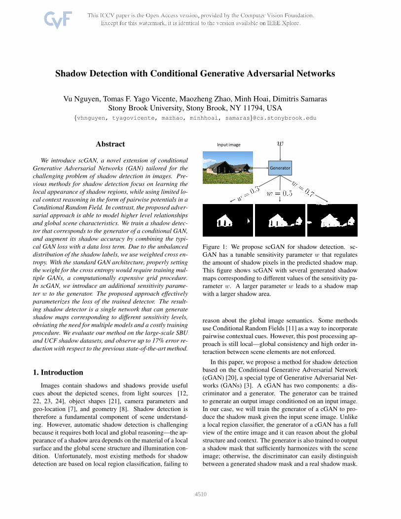
Figure 1: We propose scGAN for shadow detection. sc-

GAN has a tunable sensitivity parameter w that regulates

the amount of shadow pixels in the predicted shadow map.

This figure shows scGAN with several generated shadow

maps corresponding to different values of the sensitivity pa-

rameter w. A larger parameter w leads to a shadow map

with a larger shadow area.

reason about the global image semantics. Some methods

use Conditional Random Fields [11] as a way to incorporate

pairwise contextual cues. However, this post processing ap-

proach is still local—global consistency and high order in-

teraction between scene elements are not enforced.

In this paper, we propose a method for shadow detection

based on the Conditional Generative Adversarial Network

(cGAN) [20], a special type of Generative Adversarial Net-

works (GANs) [3]. A cGAN has two components: a dis-

criminator and a generator. The generator can be trained

to generate an output image conditioned on an input image.

In our case, we will train the generator of a cGAN to pro-

duce the shadow mask given the input scene image. Unlike

a local region classifier, the generator of a cGAN has a full

view of the entire image and it can reason about the global

structure and context. The generator is also trained to output

a shadow mask that sufficiently harmonizes with the scene

image; otherwise, the discriminator can easily distinguish

between a generated shadow mask and a real shadow mask.

4510

It is worth mentioning that cGANs have been successfully

applied to other image-to-image translation problems, in-

cluding image superresolution [15], image inpainting [25],

style transfer [16], video frame prediction [19], and future

prediction [31].

However, one drawback of cGANs is their inflexibility.

Once a cGAN has been trained, it cannot be easily adapted

to satisfy any new requirements. Particularly for shadow

detection, it will be impossible to tune the sensitivity of the

detector because there is no sensitivity parameter. For cer-

tain images and domains, this can be frustrating because

we cannot ask the detector to output fewer or more shadow

pixels. The reader might wonder whether we can simply

train a cGAN to output a continuous shadow probability

map instead of a binary mask. However the generator of

a cGAN will always generate images that are close to bi-

nary images even though we do not enforce binary output.

This is because the generator is trained to fool the discrim-

inator, and a non-binary image can be easily classified as

a fake shadow mask. The only solution would be to train

multiple cGANs for different sensitivity levels and pick the

best, at huge computational cost.

In this paper, we propose scGAN, a novel cGAN archi-

tecture with a tunable sensitivity parameter. An scGAN dif-

fers from a cGAN in multiple aspects: the network archi-

tecture, the loss function, and the training procedure. i) The

generator of an scGAN has an additional input, which is the

sensitivity parameter, as illustrated in Figure 1. ii) The train-

ing loss of the generator is augmented to include a loss term

that encourages agreement between the generator’s output

and the corresponding ground truth target image. This loss

term is based on weighted cross entropy, where the weight

corresponds to the sensitivity parameter. iii) We propose an

efficient training procedure to train the generator to respond

appropriately to different sensitivity parameter values.

To evaluate our shadow detection method we perform ex-

periments on the SBU dataset [30] which is the largest pub-

licly available shadow dataset and on the UCF dataset [32]

and observe that our proposed approach outperforms the

previous state of the art [30]. In terms of balanced error

rate we obtain a significant 17% and 12% error reduction

on SBU and UCF respectively. Moreover, we reduce the er-

ror in shadow pixels by almost 20% (SBU) and 15% (UCF)

while correctly detecting 17% (SBU) and 11 %(UCF) more

non-shadow pixels with respect to [30]. This work contains

the following contributions:

• We present the first application of adversarial training

for shadow detection.

• We develop scGAN, a novel conditional GAN archi-

tecture with a tunable sensitivity parameter that can be

efficiently trained.

• The proposed method outperforms the state-of-the-art

by a wide margin for shadow detection in the challeng-

ing SBU [30] and UCF [32] datasets.

2. Previous Work

2.1. Single image shadow detection

Single image shadow detection has been widely stud-

ied. Early work used physical models of illumination and

color. These methods, such as the illumination invari-

ant approaches of Finlayson et al. [1, 2], only work well

on high quality images [13]. For consumer photographs

and web quality images, data-driven statistical learning ap-

proaches [4, 5, 13, 28, 32] are more effective, as shown

in the two benchmark shadow datasets: UCF [32] and

UIUC [4]. These methods learn the appearance of shadow

areas from images with annotated ground truth.

There have been great advances in shadow detection in

the recent years. Khan et al. [9] were the first to use deep

learning to automatically learn features for shadow detec-

tion that significantly improved the state of the art. First,

they trained two Convolutional Neural Networks (CNNs):

one CNN is trained to label shadow regions, the other CNN

was trained to label shadow boundaries. Then, the pre-

dictions from both CNNs were combined into a unary po-

tential for a CRF that labels image pixels as shadow/non-

shadow. They also added to the CRF a pairwise poten-

tial with an Ising prior that penalizes different label assign-

ments for adjacent pixels with similar intensities. Vicente

et al. [27, 29] proposed a multikernel model for shadow re-

gion classification. The parameters and hyperparameters of

the model were efficiently optimized based on least-squares

SVM leave-one-out estimates. They also embedded the

multikernel region classifier into a CRF with added context

based pairwise potentials. Their pairwise potentials intro-

duced more contextual cues than the simple Ising prior of

Khan et al. [9]. However, these only model local interac-

tions between neighboring regions of an image. More re-

cent work of Vicente et al. [30] used a stacked CNN for

large scale shadow detection. The stacked architecture re-

fines the image level predictions of a FCN [17], pretrained

for semantic labeling, with a patch-based CNN tuned on

shadow data. This architecture achieved state-of-the-art re-

sults on several datasets. However, this approach is not

end-to-end and it requires a cumbersome two step train-

ing: firstly an FCN is trained to generate the image level

shadow-prior. The image level prior is then combined with

RGB local patches for the later training of the patch-based

CNN which produces shadow masks for the local patches.

In this approach, some more global context is considered as

the FCN makes image level predictions. However, the fi-

nal shadow predictions are made by the patch-based CNN,

which does not take into account pixels further than the

width of the patch.

4511

3. scGAN for Shadow Detection

We propose scGAN, a novel architecture that addresses

the limitations of the standard cGAN approach for shadow

detection, as explained in Section 3.1. This section de-

scribes the architecture, the training loss, and the training

procedure of scGAN.

3.1. Conditional Generative Adversarial Networks

Generative Adversarial Networks (GANs) [3], are re-

cently proposed generative models for images. A GAN con-

sists of two adversarial networks: a generator G, and a dis-

criminator D. The generator G aims to generate a realistic

image, having been given as input z, a latent random vector

sampled from some noise distribution. The discriminator

D learns to classify if a given image was generated by G(fake sample) or it is indeed a real image from the training

set. Hence, the two models compete against each other. Gaims to generate images that will be hard for D to discern

as fake, thus learning the data distribution from the training

set. Meanwhile D aims to avoid being deceived by G.

Conditional Generative Adversarial Networks

(cGANs) [20] are an extension of GANs that allows

the introduction of additional observed information (con-

ditioning variable) to both the generator (G) and the

discriminator (D). For instance, a cGAN can be applied to

the shadow detection task by using as conditioning variable

an input RGB scene image x. The generator G is trained to

output a shadow mask G(z,x) (z is an random variable for

GAN) that can realistically correspond to y, the shadows

depicted in the input image x. G learns to model the

distribution pdata(x,y) of the training data which consists

of pairs of input image x and ground-truth shadow mask y.

Then D is presented with either (x,y) or (x,G(z,x)) and

has to decide if the pair truly comes from the training data.

The objective function for the cGAN is:

LcGAN (G,D) = Ex,y∼pdata(x,y)[logD(x,y)] +

Ex∼pdata(x),z∼pz(z)[log(1−D(x, G(z,x)))]. (1)

It is possible to have a deterministic generator G. This can

be achieved by eliminating the random variable z. In this

case, the objective function of a cGAN can be simplified to:

LcGAN (G,D) = Ex,y∼pdata(x,y)[logD(x,y)] +

Ex∼pdata(x)[log(1−D(x, G(x)))]. (2)

Previous works [6, 18, 25] using cGANs often introduce

a data loss term to encourage the generated image G(x) to

be close to the ground truth image y, e.g.,

Ldata(G) = Ex,y∼pdata(x,y)||y −G(x)||2. (3)

The generator is encouraged to both fool the discrimina-

tor and produce an output that is close to the ground-truth.

Training a cGAN equates to the generator and the discrimi-

nator playing a min-max game:

minG

maxD

LcGAN (G,D) + λLdata(G). (4)

Conditional GANs provide an elegant framework for

shadow detection. A cGAN is able to effectively enforce

higher order consistencies, that cannot be modeled with

CRF pairwise terms or per pixel data loss. This is thanks

to the adversarial model’s ability to asses the joint config-

uration of input image and output mask [18]. This confers

an advantage to our method, compared to previous shadow

detection approaches.

Shadow detection is a binary classification problem with

highly unbalanced classes: typically there are significantly

fewer shadow pixels than non shadow pixels in natural im-

ages. However, good performance for both classes is de-

sired. This is often addressed by adjusting the classification

threshold accordingly, and/or setting different misclassifica-

tion costs for each class. Unfortunately, neither approaches

can be easily applied to the standard cGAN formulation.

First, because of the adversarial training, G will learn to out-

put binary values in the shadow masks, otherwise it would

be easy for the discriminator D to detect fakes (ground-

truth masks are binary). Second, although Ldata(G) can

take the form of a per class weighted loss, properly tuning

these class weights would require a grid search with mod-

els retrained over all possible weight values, potentially an

extremely computational cost.

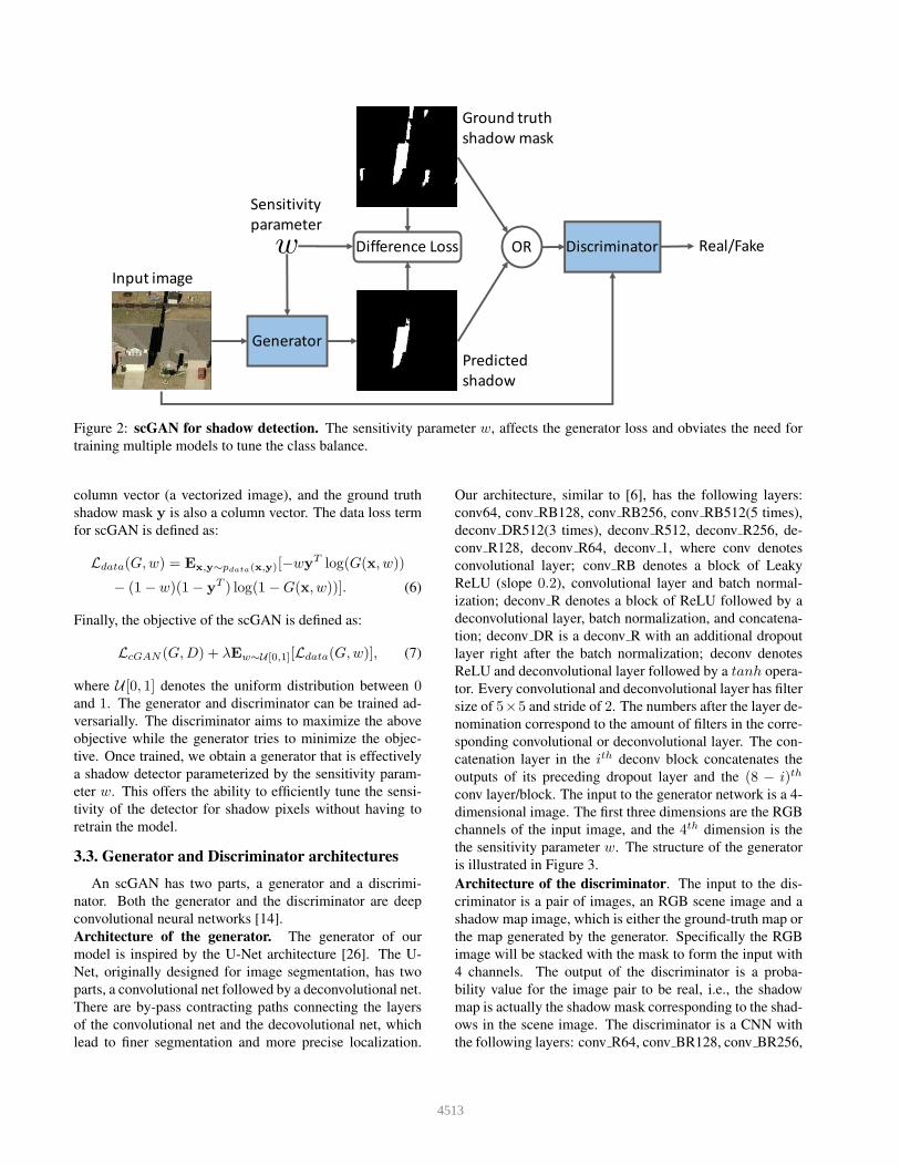
3.2. Sensitivity parameter

Compared to cGAN, scGAN has an additional sensitivity

parameter w that serves two purposes, see Figure 2. First, it

is an input of the generator G and it controls the sensitivity

of the generator. The generator G is still conditioned on the

input scene image, but a larger w will generate a predicted

shadow mask with more shadow pixels and vise versa. Sec-

ond, the parameter w is also a parameter of the loss func-

tion, weighting the relative importance of shadow and non-

shadow classes. Formally, consider a particular pixel and

suppose the ground truth value is y (y = 1 if this is a shadow

pixel and y = 0 for non-shadow pixel). Suppose the gener-

ator outputs a probability value g for this pixel (0 ≤ g ≤ 1)

being a shadow. The data loss for this pixel is defined as the

weighted cross entropy loss:

−(

wy log(g) + (1− w)(1− y) log(1− g))

. (5)

This loss is −w log(g) if y is a shadow pixel and (w −1) log(1−g) if y is a non-shadow pixel. Thus, if w ≫ 1−w,

we will penalize a wrongly classified shadow pixel much

more than a wrongly classified non-shadow pixel.

Let G(x, w) denote the predicted shadow probability

map for input image x at sensitivity level w. For mathe-

matical convenience, assume G(x, w) is represented as a

4512

Generator

DiscriminatorORDifferenceLossw

Sensitivity

parameter

Inputimage

Groundtruth

shadowmask

Predicted

shadow

Real/Fake

Figure 2: scGAN for shadow detection. The sensitivity parameter w, affects the generator loss and obviates the need for

training multiple models to tune the class balance.

column vector (a vectorized image), and the ground truth

shadow mask y is also a column vector. The data loss term

for scGAN is defined as:

Ldata(G,w) = Ex,y∼pdata(x,y)[−wyT log(G(x, w))

− (1− w)(1− yT ) log(1−G(x, w))]. (6)

Finally, the objective of the scGAN is defined as:

LcGAN (G,D) + λEw∼U [0,1][Ldata(G,w)], (7)

where U [0, 1] denotes the uniform distribution between 0and 1. The generator and discriminator can be trained ad-

versarially. The discriminator aims to maximize the above

objective while the generator tries to minimize the objec-

tive. Once trained, we obtain a generator that is effectively

a shadow detector parameterized by the sensitivity param-

eter w. This offers the ability to efficiently tune the sensi-

tivity of the detector for shadow pixels without having to

retrain the model.

3.3. Generator and Discriminator architectures

An scGAN has two parts, a generator and a discrimi-

nator. Both the generator and the discriminator are deep

convolutional neural networks [14].

Architecture of the generator. The generator of our

model is inspired by the U-Net architecture [26]. The U-

Net, originally designed for image segmentation, has two

parts, a convolutional net followed by a deconvolutional net.

There are by-pass contracting paths connecting the layers

of the convolutional net and the decovolutional net, which

lead to finer segmentation and more precise localization.

Our architecture, similar to [6], has the following layers:

conv64, conv RB128, conv RB256, conv RB512(5 times),

deconv DR512(3 times), deconv R512, deconv R256, de-

conv R128, deconv R64, deconv 1, where conv denotes

convolutional layer; conv RB denotes a block of Leaky

ReLU (slope 0.2), convolutional layer and batch normal-

ization; deconv R denotes a block of ReLU followed by a

deconvolutional layer, batch normalization, and concatena-

tion; deconv DR is a deconv R with an additional dropout

layer right after the batch normalization; deconv denotes

ReLU and deconvolutional layer followed by a tanh opera-

tor. Every convolutional and deconvolutional layer has filter

size of 5×5 and stride of 2. The numbers after the layer de-

nomination correspond to the amount of filters in the corre-

sponding convolutional or deconvolutional layer. The con-

catenation layer in the ith deconv block concatenates the

outputs of its preceding dropout layer and the (8 − i)th

conv layer/block. The input to the generator network is a 4-

dimensional image. The first three dimensions are the RGB

channels of the input image, and the 4th dimension is the

the sensitivity parameter w. The structure of the generator

is illustrated in Figure 3.

Architecture of the discriminator. The input to the dis-

criminator is a pair of images, an RGB scene image and a

shadow map image, which is either the ground-truth map or

the map generated by the generator. Specifically the RGB

image will be stacked with the mask to form the input with

4 channels. The output of the discriminator is a proba-

bility value for the image pair to be real, i.e., the shadow

map is actually the shadow mask corresponding to the shad-

ows in the scene image. The discriminator is a CNN with

the following layers: conv R64, conv BR128, conv BR256,

4513

... ...

Sensitive

ParameterGeneratedMaskInput

Image

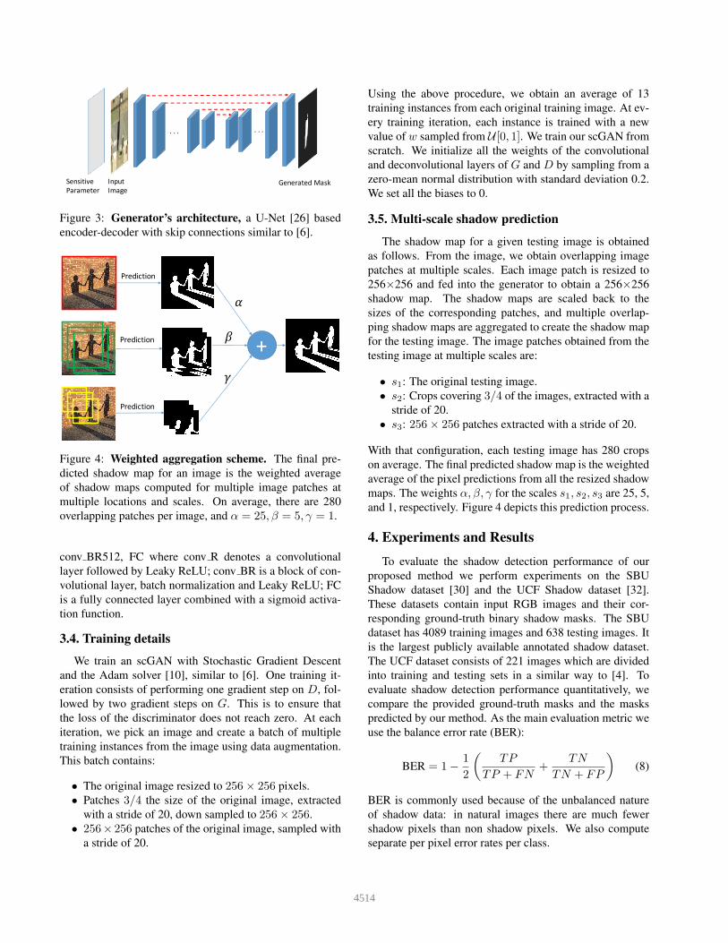
Figure 3: Generator’s architecture, a U-Net [26] based

encoder-decoder with skip connections similar to [6].

Prediction

Prediction

Prediction

+

!

"

#

Figure 4: Weighted aggregation scheme. The final pre-

dicted shadow map for an image is the weighted average

of shadow maps computed for multiple image patches at

multiple locations and scales. On average, there are 280

overlapping patches per image, and α = 25, β = 5, γ = 1.

conv BR512, FC where conv R denotes a convolutional

layer followed by Leaky ReLU; conv BR is a block of con-

volutional layer, batch normalization and Leaky ReLU; FC

is a fully connected layer combined with a sigmoid activa-

tion function.

3.4. Training details

We train an scGAN with Stochastic Gradient Descent

and the Adam solver [10], similar to [6]. One training it-

eration consists of performing one gradient step on D, fol-

lowed by two gradient steps on G. This is to ensure that

the loss of the discriminator does not reach zero. At each

iteration, we pick an image and create a batch of multiple

training instances from the image using data augmentation.

This batch contains:

• The original image resized to 256× 256 pixels.

• Patches 3/4 the size of the original image, extracted

with a stride of 20, down sampled to 256× 256.

• 256× 256 patches of the original image, sampled with

a stride of 20.

Using the above procedure, we obtain an average of 13

training instances from each original training image. At ev-

ery training iteration, each instance is trained with a new

value of w sampled from U [0, 1]. We train our scGAN from

scratch. We initialize all the weights of the convolutional

and deconvolutional layers of G and D by sampling from a

zero-mean normal distribution with standard deviation 0.2.

We set all the biases to 0.

3.5. Multi­scale shadow prediction

The shadow map for a given testing image is obtained

as follows. From the image, we obtain overlapping image

patches at multiple scales. Each image patch is resized to

256×256 and fed into the generator to obtain a 256×256

shadow map. The shadow maps are scaled back to the

sizes of the corresponding patches, and multiple overlap-

ping shadow maps are aggregated to create the shadow map

for the testing image. The image patches obtained from the

testing image at multiple scales are:

• s1: The original testing image.

• s2: Crops covering 3/4 of the images, extracted with a

stride of 20.

• s3: 256× 256 patches extracted with a stride of 20.

With that configuration, each testing image has 280 crops

on average. The final predicted shadow map is the weighted

average of the pixel predictions from all the resized shadow

maps. The weights α, β, γ for the scales s1, s2, s3 are 25, 5,

and 1, respectively. Figure 4 depicts this prediction process.

4. Experiments and Results

To evaluate the shadow detection performance of our

proposed method we perform experiments on the SBU

Shadow dataset [30] and the UCF Shadow dataset [32].

These datasets contain input RGB images and their cor-

responding ground-truth binary shadow masks. The SBU

dataset has 4089 training images and 638 testing images. It

is the largest publicly available annotated shadow dataset.

The UCF dataset consists of 221 images which are divided

into training and testing sets in a similar way to [4]. To

evaluate shadow detection performance quantitatively, we

compare the provided ground-truth masks and the masks

predicted by our method. As the main evaluation metric we

use the balance error rate (BER):

BER = 1−1

2

(

TP

TP + FN+

TN

TN + FP

)

(8)

BER is commonly used because of the unbalanced nature

of shadow data: in natural images there are much fewer

shadow pixels than non shadow pixels. We also compute

separate per pixel error rates per class.

4514

4.1. Shadow detection evaluation on SBU

We train our proposed scGAN on the SBU training

set. We evaluate the shadow detection performance of the

trained model on the SBU testing set. In Table 1, we com-

pare our results with the stackedCNN, the state-of-the-art

method on this dataset [30]. As can be seen, scGAN out-

performs stackedCNN by a wide margin; in terms of BER

we obtain a significant 17% error reduction. Moreover, sc-

GAN effectively reduces the error in shadow pixels by 19%

while also correctly detecting 17% more non shadow pixels

than the stackedCNN. These are significant improvements

over a datataset of almost 700 images depicting a wide va-

riety of scene types.

Methods BER Shadow Non Shad.

StackedCNN [30] 11.0 9.6 12.5

cGAN 13.6 20.5 6.9

scGAN (this paper) 9.1 7.8 10.4

Table 1: Evaluation of shadow detection on SBU Shadow

dataset [30]. Testing results on SBU test subset for meth-

ods training on SBU train subset. Performance measured by

Balance Error Rate(BER) and per class error rate. Our pro-

posed method achieves around 17% error reduction across

metrics with respect to the previous state of the art Stacked-

CNN [30]. Best results printed in bold.

In Fig. 5, we contrast qualitatively the performance of

scGAN and stackedCNN [30]. Compared to stackedCNN

we can observe how scGAN is not as easily fooled by the

local appearance of the dark albedo surfaces such as the

bolt, the tombstone, the blackboard and the clothing from

the scenes depicted in the first four rows. Our proposed

method is also more precise in detecting shadows cast on

brighter materials such as the snow scene in the fifth row.

We show additional qualitative examples for challenging

scenes in Figure 7. These images present some filter/lens

effects, locally ambiguous appearance, and poor illumina-

tion conditions, respectively.

4.2. Shadow detection evaluation on UCF

We also evaluate our method for the cross-dataset

shadow detection task. In this experiment, we evaluate the

proposed scGAN model trained on the SBU training set

for shadow detection, on the UCF testing set [32]. This

a very challenging task as the SBU training set does not

overlap with the UCF data sets. In Table 2, we compare to

stackedCNN [30], the state of the art method for the cross

dataset task on UCF. We conducted two experiments, one

with the model trained from UCF-Training, the other from

SBU-Training. In both experiments, we achieved better re-

sults with 6% decrease of BER in the UCF-trained model

and 12% decrease of BER in the SBU-trained model. Re-

markably, the scGAN trained on SBU obtains better testing

performance in UCF, compared to the stackedCNN method

actually trained on the UCF training set itself.

Method Training Set BER Shadow Non Shad.

stackedCNN [30] UCF-Train 11.6 10.4 12.6

scGAN (proposed) UCF-Train 10.9 10.4 11.4

stackedCNN [30] SBU-Train 13.0 9.0 17.1

scGAN (proposed) SBU-Train 11.5 7.7 15.3

Table 2: Comparison of shadow detection results on

UCF testing set. In terms of BER, our proposed method

outperforms state of the art stackedCNN[30] by 6% and

12%, when training with UCF-Training and SBU-Training

respectively.

4.3. Effects of Sensitivity Parameters

To illustrate the effects of the sensitivity parameter w in

the proposed scGAN method, we evaluate shadow detec-

tion performance on the SBU testing set [30] for different

values of w. As shown in Table 3, testing with higher val-

ues of w effectively increases the sensitivity of the trained

models towards shadow pixels (minority class). In terms of

Balance Error Rate (BER), the scGAN model achieves best

performance for w = 0.7.

w BER Shadow Non Shad.

0.3 10.6 15.4 5.8

0.5 9.7 12.4 7.0

0.7 9.0 8.7 9.4

0.8 9.1 7.8 10.4

0.9 10.6 4.7 16.5

Table 3: Influence of the sensitivity parameter in shadow

detection. The proposed scGAN model is trained on SBU

Shadow dataset [30], testing with different values of sensi-

tivity parameter w. Performance measured by BER and per

class error rate on SBU testing set. Shadow error rate de-

creases when the sensitivity parameter increases. The best

overall performance is achieved for 0.7.

4.4. scGAN vs cGAN

We compare the proposed scGAN with a cGAN model

of our architecture on the SBU dataset. The cGAN version

is obtained by setting λ as zero in the objective function,

hence training without any data loss term. Shadow detec-

tion results with the cGAN deteriorate considerably when

testing in SBU. The BER drops to 13.6 which is a 49% de-

crease compared to scGAN. This demonstrates the benefits

4515

(a) Input Image (b) Ground-truth Mask (c) stackedCNN [30] (d) scGAN(ours)

Figure 5: Comparison of shadow detection on SBU dataset. (a) Input image. (b) Shadow ground-truth mask. (c) Predicted mask by the

stackedCNN[30]. (d) Predicted mask by our proposed method scGAN.

of our proposed approach. In Figure 6, we show qualitative

comparisons of scGAN and cGAN. In the 2nd row of Ta-

ble 1,we can see that, unsurprisingly, cGAN prefers to clas-

sify more non-shadow pixels correctly than shadow pixels

(which is by far the smallest class).

5. Conclusions

In this paper, we have formulated the shadow detec-

tion problem in a generative adversarial framework. We

have shown how to parameterize the loss function to handle

severely unbalanced training sets without needing to train

multiple models for tuning. Our method significantly re-

duced errors when tested on the most challenging available

shadow datasets. The proposed method can also be applied

on other classification problems with unbalanced classes

such as infrastructure inspection problems (e.g., road sur-

face condition datasets).

Acknowledgements This work was supported by the Stony

Brook University SensorCAT, a gift from Adobe, the Part-

ner University Fund 4DVision project, and the SUNY 2020-

Infrastructure, Transportation and Security Center.

References

[1] G. Finlayson, M. Drew, and C. Lu. Entropy minimization for

shadow removal. International Journal of Computer Vision,

2009.[2] G. Finlayson, S. Hordley, C. Lu, and M. Drew. On the re-

moval of shadows from images. IEEE Transactions on Pat-

tern Analysis and Machine Intelligence, 2006.

(a) Input Image (b) cGAN (c) scGAN

Figure 6: Detection results scGAN vs cGAN. (a) Input

image. (b) cGAN prediction. (c) scGAN prediction.

[3] I. J. Goodfellow, J. Pouget-Abadie, M. Mirza, B. Xu,

4516

(a) Input Image (b) Ground-truth Mask (c) Predicted Mask

Figure 7: Shadow detection examples on the SBU dataset. (a) Input image. (b) Shadow ground-truth mask. (c) Predicted

mask by our proposed method scGAN.

4517

D. Warde-Farley, S. Ozair, A. C. Courville, and Y. Bengio.

Generative adversarial networks. In Advances in Neural In-

formation Processing Systems, 2014.[4] R. Guo, Q. Dai, and D. Hoiem. Single-image shadow detec-

tion and removal using paired regions. In Proceedings of the

IEEE Conference on Computer Vision and Pattern Recogni-

tion, 2011.[5] X. Huang, G. Hua, J. Tumblin, and L. Williams. What char-

acterizes a shadow boundary under the sun and sky? In

Proceedings of the International Conference on Computer

Vision, 2011.[6] P. Isola, J. Zhu, T. Zhou, and A. A. Efros. Image-to-image

translation with conditional adversarial networks. In Pro-

ceedings of the IEEE Conference on Computer Vision and

Pattern Recognition, 2017.[7] I. Junejo and H. Foroosh. Estimating geo-temporal location

of stationary cameras using shadow trajectories. In Proceed-

ings of the European Conference on Computer Vision, 2008.[8] K. Karsch, V. Hedau, D. Forsyth, and D. Hoiem. Rendering

synthetic objects into legacy photographs. ACM Transac-

tions on Graphics, 2011.[9] H. Khan, M. Bennamoun, F. Sohel, and R. Togneri. Auto-

matic feature learning for robust shadow detection. In Pro-

ceedings of the IEEE Conference on Computer Vision and

Pattern Recognition, 2014.[10] D. P. Kingma and J. Ba. Adam: A method for stochastic

optimization. In Proceedings of the International Conference

on Learning Representations, 2015.[11] J. D. Lafferty, A. McCallum, and F. C. N. Pereira. Con-

ditional random fields: Probabilistic models for segmenting

and labeling sequence data. In Proceedings of the Interna-

tional Conference on Machine Learning, 2001.[12] J.-F. Lalonde, A. Efros, and S. Narasimhan. Estimating natu-

ral illumination from a single outdoor image. In Proceedings

of the European Conference on Computer Vision, 2009.[13] J.-F. Lalonde, A. A. Efros, and S. G. Narasimhan. Detecting

ground shadows in outdoor consumer photographs. In Pro-

ceedings of the European Conference on Computer Vision,

2010.[14] Y. LeCun, B. Boser, J. S. Denker, and D. Henderson. Back-

propagation applied to handwritten zip code recognition.

Neural Computation, 1(4):541–551, 1989.[15] C. Ledig, L. Theis, F. Huszr, J. Caballero, A. Cunning-

ham, A. Acosta, A. Aitken, A. Tejani, J. Totz, Z. Wang,

and W. Shi. Photo-realistic single image super-resolution us-

ing a generative adversarial network. In Proceedings of the

IEEE Conference on Computer Vision and Pattern Recogni-

tion, 2017.[16] C. Li and M. Wand. Precomputed real-time texture synthesis

with markovian generative adversarial networks. In Proceed-

ings of the European Conference on Computer Vision, 2016.[17] J. Long, E. Shelhamer, and T. Darrell. Fully convolutional

networks for semantic segmentation. In Proceedings of the

IEEE Conference on Computer Vision and Pattern Recogni-

tion, 2015.[18] P. Luc, C. Couprie, S. Chintala, and J. Verbeek. Semantic

segmentation using adversarial networks. In NIPS Workshop

on Adversarial Training, 2016.[19] C. C. M. Mathieu and Y. LeCun. Deep multi-scale video pre-

diction beyond mean square error. In Proceedings of the In-

ternational Conference on Learning Representations, 2016.[20] M. Mirza and S. Osindero. Conditional generative adversar-

ial nets. In NIPS Deep Learning and Representation Learn-

ing Workshop, 2014.[21] S. I. Okabe, T and Y. Sato. Attached shadow coding: es-

timating surface normals from shadows under unknown re-

flectance and lighting conditions. In Proceedings of the Eu-

ropean Conference on Computer Vision, 2009.[22] A. Panagopoulos, D. Samaras, and N. Paragios. Robust

shadow and illumination estimation using a mixture model.

In Proceedings of the IEEE Conference on Computer Vision

and Pattern Recognition, 2009.[23] A. Panagopoulos, C. Wang, D. Samaras, and N. Paragios. Il-

lumination estimation and cast shadow detection through a

higher-order graphical model. In Proceedings of the IEEE

Conference on Computer Vision and Pattern Recognition,

2011.[24] A. Panagopoulos, C. Wang, D. Samaras, and N. Paragios.

Simultaneous cast shadows, illumination and geometry in-

ference using hypergraphs. IEEE Transactions on Pattern

Analysis and Machine Intelligence, 2013.[25] D. Pathak, P. Krahenbuhl, J. Donahue, T. Darrell, and

A. Efros. Context encoders: Feature learning by inpainting.

In Proceedings of the IEEE Conference on Computer Vision

and Pattern Recognition, 2016.[26] O. Ronneberger, P.Fischer, and T. Brox. U-net: Convolu-

tional networks for biomedical image segmentation. In Med-

ical Image Computing and Computer-Assisted Intervention

(MICCAI), 2015.[27] T. F. Y. Vicente, M. Hoai, and D. Samaras. Leave-one-out

kernel optimization for shadow detection. In Proceedings of

the International Conference on Computer Vision, 2015.[28] T. F. Y. Vicente, M. Hoai, and D. Samaras. Noisy label recov-

ery for shadow detection in unfamiliar domains. In Proceed-

ings of IEEE Conference on Computer Vision and Pattern

Recognition, 2016.[29] T. F. Y. Vicente, M. Hoai, and D. Samaras. Leave-one-out

kernel optimization for shadow detection and removal. IEEE

Transactions on Pattern Analysis and Machine Intelligence,

2017.[30] T. F. Y. Vicente, L. Hou, C.-P. Yu, M. Hoai, and D. Sama-

ras. Large-scale training of shadow detectors with noisily-

annotated shadow examples. In Proceedings of the European

Conference on Computer Vision, 2016.[31] Y. Zhou and T. L. Berg. Learning temporal transformations

from time-lapse videos. In Proceedings of the European

Conference on Computer Vision, 2016.[32] J. Zhu, K. Samuel, S. Masood, and M. Tappen. Learning

to recognize shadows in monochromatic natural images. In

Proceedings of the IEEE Conference on Computer Vision

and Pattern Recognition, 2010.

4518