shape coding for arbitrarily shaped object€¦ · · 2009-03-19shape coding for arbitrarily...
TRANSCRIPT

Shape Coding For Arbitrarily Shaped Object
By
Heechan Park
Supervised By
Dr. Graham Martin
A Final Year Project Report
in Partial Fulfillment of the
Requirements for the Degree of
BACHELOR OF SCIENCE
Department of Computer Science
University of Warwick
Coventry,CV4 7AL, United Kingdom
April 2004

2

3
Abstract
New functionalities in digital communication are demanded in multimedia applications such
as content-based storage and retrieval, studio and television postproduction, and mobile
multimedia. The functionalities enable to handle individual objects separately, thus allowing
scalable transmission as well as interactive scene re-composition by the receiver. Unlike
existing frame-based standards, the corresponding coding schemes need to encode shape
information explicitly.
In this report, the existing shape intra- / inter-coding schemes are reviewed. A highly
efficient contour-based coding scheme employing directionality and anisotropy is proposed
offering at most 20% gain over the most efficient lossless shape coding scheme. Also,
various suggestions are presented regarding pre-processing, block-based compatibility,
rate-distortion control capability and progressive transmission.
Keywords: Object oriented video coding, MPEG-4, Contour based Shape Coding, Multiple
Grid Chain Coding, Radon Transform, Quadtree, Hybrid Coding, Scalable coding

4

5
Acknowledgement
The author wishes to express sincere thanks to supervisor, Dr. Graham Martin for his
valuable guidance and advices, to Eunjung and my parents for enormous supports, and also
to PhD student Nick and Vincent for valuable suggestions.
The author acknowledges that software, JMatLink, that enables to use Matlab’s
computational engine in Java application is used in an implementation of Radon / Quadtree
hybrid coding scheme. A full distribution of the software can be found at :
http://www.held-mueller.de/JMatLink/

6

7
CONTENTS
LIST OF FIGURES ................................................................................................................... 10
LIST OF TABLES ..................................................................................................................... 12
1 INTRODUCTION ...................................................................................................14
1.1 Compression as Key Technology............................................................................. 14
1.2 Interactivity and Object-Based Coding .................................................................... 15
1.3 Shape Coding and Project Scope ............................................................................. 16
1.4 Report Organisation................................................................................................. 17
2 SOURCE CODING PRINCIPLES ............................................................................20
2.1 Shannon’s Source Coding Theorem......................................................................... 20
2.2 Redundancy.............................................................................................................. 23
2.3 Compression Algorithm ........................................................................................... 25
2.3.1 Run Length Coding............................................................................................ 25
2.3.2 Statistical Coding .............................................................................................. 26
2.3.3 Dictionary-Based Coding................................................................................... 29
3 VIDEO CODING.....................................................................................................32
3.1 Waveform-Based Techniques ................................................................................... 32
3.1.1 Image Coding .................................................................................................... 32
3.1.2 Video Coding ..................................................................................................... 34
3.2 Object-Based Coding Techniques ............................................................................ 35
3.2.1 Image Coding .................................................................................................... 35
3.2.2 Video Coding ..................................................................................................... 36
3.3 Fractal-Based Techniques........................................................................................ 38
3.3.1 Image Coding .................................................................................................... 38
3.3.2 Video Coding ..................................................................................................... 39
3.4 Model-Based Coding ................................................................................................ 40

8
4 MPEG-4 STANDARD: natural video ......................................................................42
4.1 Structure and syntax................................................................................................ 43
4.2 Shape coding............................................................................................................ 45
4.3 Motion coding .......................................................................................................... 49
4.4 Texture coding ......................................................................................................... 53
4.5 H.264 and MPEG-2, -47 ........................................................................................... 54
5 SHAPE CODING ....................................................................................................58
5.1 Literature Review .................................................................................................... 58
5.1.1 Bitmap-BasedCoding ......................................................................................... 59
5.1.2 Intrinsic Shape Coding...................................................................................... 61
5.1.3 Contour-Based Coding ...................................................................................... 64
5.1.3.1 Chain Coding ............................................................................................ 64
5.1.3.1.1 Lossless Coding...................................................................... 64
5.1.3.1.2 Lossy Coding .......................................................................... 68
5.1.3.2 Geometrical Representation..................................................................... 69
5.1.3.2.1 Polygonal Approximation ....................................................... 70
5.1.3.2.2 Higher Order Approximation ................................................. 71
5.2 Multiple Grid Chain Code ........................................................................................ 73
5.2.1 Quasi-lossless Shape Coding ............................................................................. 74
5.2.2 Improvement ..................................................................................................... 77
5.2.2.1 Approach1: Improve 3x3 Cell ................................................................... 77
5.2.2.2 Approach2: Polygonal Chain Code ........................................................... 79
5.2.2.3 Approach3: Directionality and Anisotropy ............................................... 81
5.2.2.4 Approach4: Flexible Directionality........................................................... 86
5.2.2.5 Evaluation................................................................................................. 89
5.2.3 Pre-Processing................................................................................................... 94
5.3 Hybrid Coding.......................................................................................................... 96
5.3.1 Radon Transform / Quadtree Hybrid Coding .................................................... 96
5.3.2 Chain Code / Quadtree Hybrid Coding............................................................ 102
5.4 Inter-Frame Coding................................................................................................ 104
5.4.1 Motion-Based Prediction Schemes.................................................................. 105
5.4.2 Entropy-Based Prediction Schemes ................................................................ 107
5.4.3 Chain-Based Contour Compensation Schemes ............................................... 107

9
6 COMMUNICATION SYSTEM ISSUES..................................................................109
6.1 Scalable Coding ..................................................................................................... 110
6.2 Progressive Transmission ...................................................................................... 111
6.3 Bit-Rate Estimation ................................................................................................ 112
7 SUMMARY AND CONCLUSION ..................................................................................114
7.1 Summary of Shape Coding Methods and Discussion............................................. 114
7.2 Topics for Future Research.................................................................................... 117
7.3 Contributions and Author’s Assessment ................................................................ 119
APPENDIX.................................................................................................................122
A. Software Documentation........................................................................................... 122
A.1 Coder Implementation....................................................................................... 122
A.2 Organisation and Compilation........................................................................... 124
B. Graphical Experimental Results................................................................................ 126
C. Probability of Symbols and Codewords..................................................................... 130
D. Bibliography .............................................................................................................. 134

10
LIST OF FIGURES
Figure 2.1 Five different representations of the same information........................... 21
Figure 2.2 An example of Huffman coding tree......................................................... 27
Figure 2.3 An example of Arithmetic coding process ................................................ 28
Figure 3.1 General block diagram of predictive coding ............................................ 33
Figure 3.2 General block diagram of a transform-based scheme.............................. 33
Figure 3.3 Example of Object-based decoding in MPEG-4 ........................................ 36
Figure 3.4 Object composition................................................................................... 37
Figure 3.5 Koch curve................................................................................................ 38
Figure 3.6 Overview of model-based coder structure ............................................... 40
Figure 4.1 Hierarchical description of a visual scene ............................................... 44
Figure 4.2 Alpha plane and corresponding bounding box......................................... 46
Figure 4.3 CAE templates.......................................................................................... 46
Figure 4.4 Three modes of VOP coding ..................................................................... 50
Figure 4.5 Motion vector prediction.......................................................................... 51
Figure 4.6 Texture coding ......................................................................................... 53
Figure 5.1 Skeleton decomposition ........................................................................... 62
Figure 5.2 Hybrid macroblock / Quadtree structure ................................................. 63
Figure 5.3 Contour representation and chain code................................................... 65
Figure 5.4 MGCC, Hexagonal grid and 6 connectivity chain .................................... 69
Figure 5.5 Polygonal approximation.......................................................................... 70
Figure 5.6 Type of MGCC cells .................................................................................. 74
Figure 5.7 Ambiguities introduced by MGCC............................................................ 75
Figure 5.8 Example of the MGCC coding scheme ..................................................... 76
Figure 5.9 Vertex -based cell ..................................................................................... 78
Figure 5.10 Diagonally halved cell and coding process .............................................. 78
Figure 5.11 Polygonal Approximation and Chain codes .............................................. 80
Figure 5.12 Simplified cells ......................................................................................... 80
Figure 5.13 New cell types .......................................................................................... 83
Figure 5.14 Example of the proposed coding scheme................................................. 85
Figure 5.15 Further ambiguity introduced by elongation ........................................... 86
Figure 5.16 Diagonal direction .................................................................................... 87
Figure 5.17 Diagonally-directed cells .......................................................................... 87
Figure 5.18 2x3 cell as a basic structure..................................................................... 88

11
Figure 5.19 Template for approach 4 .......................................................................... 88
Figure 5.20 Coding Scheme Screenshot...................................................................... 89
Figure 5.21 Auxiliary codewords ................................................................................. 91
Figure 5.22 2 x 3 cell types.......................................................................................... 92
Figure 5.23 Contour reconstruction of 10th frame of children sequence ................... 94
Figure 5.24 Illustration of pre-processing ................................................................... 95
Figure 5.25 Radon transform....................................................................................... 97
Figure 5.26 Smallest sub block.................................................................................... 99
Figure 5.27 Macroblock/Quadtree structure example ................................................ 99
Figure 5.28 Radon/Quadtree hybrid coding and reconstructed image ..................... 101
Figure 5.29 Various size of MGCC cell ...................................................................... 102
Figure 5.30 Chain code / Quadtree hybrid coding..................................................... 103
Figure 5.31 Prune tree segmentation and Prune-Join tree segmentation ................. 103
Figure 5.32 Overlapped contour image ..................................................................... 104
Figure 5.33 Chain -based contour compensation scheme ......................................... 108
Figure 6.1 Scalable coding based on MGCC ........................................................... 111
Figure 6.2 Progressive transmission based on chain code...................................... 112
Figure 6.3 Correlation between Eccentricity and Bit rate ...................................... 113
Figure A.1 Static Modelling ..................................................................................... 123
Figure A.2 Unnaturally Reconstructed Contour ...................................................... 123

12
LIST OF TABLES Table 4.1 BAB coding modes.................................................................................... 47
Table 4.2 List of BAB sizes for CAE ......................................................................... 49
Table 4.3 Summary of present standards for video compression ............................ 56
Table 5.1 Description of cells in Figure 5.8 ............................................................. 77
Table 5.2 Selection rules.......................................................................................... 84
Table 5.3 Description of cells in Figure 5.14 ........................................................... 85
Table 5.4 Experimental results ................................................................................ 90
Table 5.5 Selection rules adapted for 2 x 3 cell structure ....................................... 92
Table 5.6 Threshold values for each block size...................................................... 100
Table 5.7 Experimental result for Radon / Quadtree hybrid coding ...................... 100

13

14
Chapter 1
Introduction
1.1 Compression as Key Technology
A new era of digital communication has been opened with the success in micro-electronics
and computer technology coupled with the creation of networks operating with various
channel capacities. Visual information is becoming a ubiquitous part of such communication
that is proved by a huge increase in the exchange of images via networks and also by
applications such as video conferencing and mobile videophone. However, the storage and
communication requirements for visual data can be excessive, particularly if true colour
and a high perceived image quality are desired. For instance, storage problems are
particularly acute in remote sensing applications; the scenes imaged by Earth-orbiting
satellites typically have widths and heights of several thousand pixels, and there may be
several bands representing the different wavelengths in which images are acquired. The
raw data for a single scene therefore requires several hundred megabytes of storage space.
A sequence of such images presents perhaps the most serious storage problems of all. A
one minute sequence of full colour video data occupies over 1.5 gigabytes when in digital
form. Obviously, transmitting such data over network is one of most bandwidth-consuming
modes of communication.

15
The availability and demand for visual communication continue to outpace increases in
channel capacity and storage. Hence, highly efficient compression technique to reduce the
global bit rate drastically, even in the presence of growing communications channels
offering increased bandwidth, is a key requirement due to the vast amount of data
associated with visual information and its importance is not likely to diminish. A typical
video compression standard like MPEG-1, MPEG2, and H.261 uses transform-
based/predictive coding method to serve the requirement; to reduce the amount of bits
required to represent the images while preserving the visual quality to the extent that
losses are not noticeable to the human visual perception. However, those coding methods
do not offer any interactivity, which is requited by emerging applications, Section 1.2, with
users.
1.2 Interactivity and Object-Based Coding
New functionality, interactive contents with users, in addition to the conventional frame-
based compression provided by the standards are required for new applications.
Applications like content -based storage and retrieval, composition of video objects into
augmented reality, mobile multimedia share one common requirement: video content has to
be easily accessible on an object basis.
Given the application requirements, video objects have to be described not only by
texture but also by shape. The importance of shape for video objects has been realized early
on by the broadcast and movie industry by employing the so-called chroma-keying
technique. Coding algorithms like object-based analysis-synthesis coding [1] use shape as a
parameter in addition to texture and motion for describing moving video objects. Second
generation coding segments an image into regions and describes each region by texture

16
and shape [2]. The purpose of using shape was to achieve high fidelity of the reconstructed
image and to increase coding efficiency both by reducing pixels to be considered for texture
and motion coding, as well as to provide an object-based video representation by which new
functionality may be incorporated naturally. Therefore, object-based coding is a viable
alternative to the traditional coding scheme in terms of both object-based representation
and compression efficiency. The imminent video coding standards such as MPEG-4 and
H.263 adopted object-based coding. However, efficient encoding of shape, (Section 1.3) is
becoming increasingly important, since the shape information occupies a large portion of
the total bit rate [3].
1.3 Shape Coding and Project Scope
Shape Coding Techniques
There exist two main classes of shape coding techniques, namely bitmap-based and
contour-based coding. Each class of the techniques has different characteristics. The
Context-based Arithmetic Encoding (CAE), one of the bitmap-based coding techniques, was
adopted by MPEG-4 standards [3]. However, its efficiency exploiting spatial redundancy of
a frame is sub-optimal while it offers high efficiency for inter-frame coding. On the other
hands, contour-based coding methods provide highly efficient representation for contour
shape of object, but it is not adequate for temporal coherence exploitation between frames.
The contour-based coding methods consist of chain codes, representing contours by
chain of adjacent boundary pixels, and geometrical approximation, using a set of
representative vertices that are then used to reconstruct the contour via line or spline
segments. Among such methods, so-called Multiple Grid Chain Code (MGCC) offers the best

17
lossless coding efficiency by relaxing lossless constraint and minimising distortions [45].
However, inter-cell coherence is not fully exploited in the scheme.
Project Scope
The initial goal of this project was improving the MGCC by reflecting the un-captured
coherence. We have taken various approaches to improve the MGCC, which are described
in Section 5.2.3.We propose an improved version of MGCC, outperforming the MGCC by
20% in terms of bit rate while offering even lower distortion rate. The goal was extended to
investigate into further efficiency improvement as well as communication issues.
As extended part of the project, first of all, we explore a few contour-based hybrid
schemes utilising a Quadtree structure, Radon transform and the MGCC to facilitate better
compatibility with the conventional block-based motion and texture coding scheme.
Secondly, as mentioned the contour-based methods suffer from sub-optimality of inter-
frame coding efficiency, we suggest a research direction exploiting temporal redundancy
based on entropy and contour compensation preserving contour-based coding structure.
Finally, reliable transmission with limited delay constraints is an essential part in
digital communication. We discuss problems of robust communication when errors do
occur. We suggest a research direction for scalability and progressive transmission of
chain-based shape coding as well as bit rate estimation.
1.4 Report Organisation
In this report, we discuss major shape coding techniques described in literature and review
their coding efficiency and related communication issues. The structure of the paper is as
follows.

18
Chapter 2 start by reviewing source coding principles which are not specific to
image coding, but fundamentally important.
Chapter 3 outlines the major classes of video coding techniques. Object-based
coding is briefly overviewed in light of interactivity with object feature. The
problems tackled are also described in this chapter.
Chapter 4 introduces recent advance and direction in block-based coding, also
illustrates the structure of MPEG-4 standard : natural video coding
Chapter 5 reviews shape coding techniques and presents MGCC improvement and
various suggestions
Section 5.1 describes the main classes of intra mode shape coding methods;
bitmap-based coding methods, implicit shape coding principle, and contour-
based coding techniques with detailed descriptions of chain code, variants of
the same techniques and Geometrical lossy representation methods.
Section 5.2 presents Multiple Grid Chain Code (MGCC) relaxing lossless
constraint in details. An improved MGCC employing the directionality and the
anisotropy is described presented. A pre-processing technique based on
Modified Differential Chain Code (MDCC) is also suggested in this section.
Section 5.3, extended parts of the project onward this section, suggests a
hybrid coding scheme based on Radon Transform and Quadtree structure as
well as Chain and Quadtree integrated method.
Section 5.4 discusses exploiting the temporal correlation between successive
instances of the same object in order to enhance compression efficiency. A
scheme using contour compensation is suggested.
Chapter 6 examines communication issues in connection with Joint source /
channel coding principle and suggests techniques for scalable coding of contour
object, for progressive transmission and finally for bit estimation using
Eccentricity.

19
Chapter 7 concludes the report with brief summary of the content and discussions
of the contribution of this project. The topics for possible direction of future
research and development are presented. Finally, a brief self-assessment
remarking the project is followed.

20
Chapter 2
Source Coding Principles
This chapter is dedicated to source coding principles which are not specific to visual data
coding, but fundamentally important nevertheless. We review Shannon’s source coding
theorem, then discuss various kinds of redundancy resides on image and video and finally
introduce compression algorithm exploiting such redundancy.
2.1 Shannon’s Source Coding Theorem
Data and Information
Data compression addresses the problem of reducing the amount of data required to
represent a source, so that it can be stored or transmitted more efficiently. First of all, we
must make a clear distinction between data and information. Data are the means by which
information is conveyed. Various amounts of data can be used to convey the same amount
of information. Consider, for example, Figure 2.1. This shows ways of representing the
meaning of number ‘five’ using different amounts of data. Clearly, the binary integer
representation is vastly more efficient than the pictorial representation.

21
Figure 2.1Five different representations of the same information meaning five. From left to
right and top to bottom: English word using ASCII character set (32 bits); a single ASCII
digit(8 bits); a picture of dice(101,632 bits); Korean word using ISO-2022-KR (16bits);
binary integer (3 bits)
Entropy
In 1948, Claude E. Shannon introduced, in his source coding theorem [4],Entropy, or
average self-information, measures the uncertainty of a source and hence provides a
measure of the information it could reveal.
Consider, information source, X which emits, at time , a symbol from
with symbol probability, which satisfies expression below
(1.1)
The entropy of X can be defined as below
(1.2)
and it satisfies following properties :
I. A source whose output is known produces no information

22
(1.3)
II. The maximum information a source can produce is just logarithm of the alphabet size.
(1.4)
If the symbols are all equiprobable, , then the inequality becomes
equality in (1.4).
III. Entropy, considered as a function of the probability distribution, is convex.
Source Coding Theorem
Shannon relates entropy, to the minimum number of bits required to represent a
source without much loss as stated in the box below. Hence, if more data are used than is
strictly necessary, , then we say that there is redundancy in the dataset. The source
redundancy is given by
(1.5)
If the source is not independent and identically distributed, but it is stationary with
memory, then a similar theorem applies with the entropy replaced with the entropy
rate,
Shannon’s Source coding theorem A source that produced independent and identically distributed random variables with entropy, can be encoded with arbitrarily small error probability at any rate R in bits per source output if . Conversely, if , the error probability will be bounded away from zero, independent of the complexity of coder and decoder.

23
(1.6)
where the conditional entropy is defined as
(1.7)
The more the source produces outputs the more one knows about the source and the more
one can compress.
The source coding theorem proves existence of source coding techniques that achieve rates
close to the entropy but does not provide any algorithms or ways to construct such codes.
There are a number of source coding algorithms for discrete valued sources that come close
to Shannon's bound. In the next section, we shall focus on redundancies found in visual
data and the algorithms with respect to such redundancies.
2.2 Redundancy in Visual Data and Compression
Redundancy
In a visual data, four basic types of redundancy can be identified. Coding redundancy arises
when the representation chosen for the pixel values of an image is not the most efficient
that is possible. For instance, an 8-bit coding scheme has the capacity to represent 256
distinct levels of intensity in an image. However, if there are only 16 different grey levels in
a particular image, such an image exhibits coding redundancy because it could be
represented using a 4-bit coding scheme.
A second type of redundancy often present in images in interpixel redundancy. This
arises because the values of a pixel and its immediate neighbours are often strongly

24
correlated. This means that the value at a pixel can be predicted with a reasonable degree
of accuracy from values of its neighbours. Consequently, the amount of information
conveyed by a n individual pixel is relatively small, and the amount of data that is needed to
represent that pixel is correspondingly small.
The third type of redundancy is psychovisual redundancy. This arises because not all
the information present in an image is of equal importance to the human visual system. For
example, there are upper limits on the number of quantization levels that can be easily
distinguished by eye, and on the spatial frequencies that can be detected by the eye.
There is a fourth type of redundancy, when video data are available, interframe
redundancy. This is the temporal equivalent of interpixel redundancy. Video frame rates are
sufficiently high that the change in a pixel’s value from frame to frame is typically very
small over the majority of the frame. Data compression can be achieved by encoding the
relatively small number of changes that occur from frame to frame, rather than each frame
in its entirety.
Lossless and Lossy Compression
We have discussed kinds of redundancy which could reside in visual data. Compression
algorithms exploiting such redundancy fall into two groups, namely, lossless and lossy.
Lossless compression techniques are designed to remove redundancy when data are stored
or transmitted. The reconstruction from the compressed dataset is identical to the original,
i.e., all of the information originally present in the source has been preserved by
compression. Higher compression is possible using lossy compression techniques, which
normally are applied to image dataset. The lossy image compression schemes discard some
of the meaningless information, such as psychovisual redundancy presented in the image.
The reconstructed image will not be identical to the original image, although the difference
need not be clearly visible to the human eye.

25
2.3 Compression Algorithm
We shall concentrate on general algorithms that remove redundancy with lossless
constraint. Firstly, Run length Coding (RLC) which is very useful for binary data,
particularly binary image containing long runs of ones of zeros will be introduced. Two
popular statistical coding methods will be covered, namely Huffman coding and Arithmetic
coding. Huffman Coding is one of the simplest variable length coding schemes. Arithmetic
Coding is a relatively new variable length coding scheme that can combine the best
features of Huffman and run-length coding, and also adapt to data with non-stationary
statistics. Lastly, dictionary-based coding methods that have been widely used in many text
compression applications are discussed.
2.3.1 Run Length Coding
The technique of run length coding (RLC) exploits the high interpixel redundancy that
exists in relatively simple images. In RLC, we look for grey levels that repeat along ach row
of the image. A run of consecutive pixels whose grey levels are identical is replaced with
two values: the length of the run and the grey level of all pixels in the run. Hence, the
sequence {1, 1, 1, 1} becomes {4, 1}.
Note that, if the run is of length 1, RLE replaces one value with a pair of values. It is
therefore possible for RLC to increase the size of the dataset in images where runs of
length 1 are numerous. This might be the case in noisy or highly textured images. For this
reason, RLC is most useful for the compression of binary images or very simple greyscale
image

26
2.3.2 Statistical coding
Statistical coding techniques remove the coding redundancy in an image. This redundancy
exists because fixed-length (typically 8 bits) codewords are used to represent pixel values.
As stated earlier, according to the Shannon’s information theory, codewords that occur
rarely convey more information than codewords that occur frequently in the data. An
optimal coding scheme will use more bits for the rare codewords and fewer bits for the
frequent codewords. Compression scheme assuming a certain model on the statistics of
pixels in image will be covered in Section 3.1.
Huffman Coding
Huffman coding is simply a particular way of choosing the codewords, such that the
average bit length of the codewords is as close as possible to the entropy of the image. We
start by ranking pixel values in decreasing order of their probability. We then pair the two
values with the lowest probabilities, labelling one of them with 0 and the other with 1. Their
probabilities are summed to give the probability of either value from the pair occurring in
the image. We then identify the next two lowest probabilities from the current set of
individual values or paired values. These are then paired, with one member of the pair
labelled 0 and 1, and so on. The process continues, building up a tree-like structure of
paired values as depicted in Figure 2.2.

27
Figure 2.2An example of Huffman tree for 8-bit greyscale image where digits in bold and
italic represents intensity of a pixel and codeword respectively.
Following this tree from each leaf node to the root gives a sequence of bits that, when
reversed, represent the codeword for the value at the leaf node. Since the length of the bits
are always integers, up to 1 bit per symbol can be redundant. It is only optimal when all
symbols’ probabilities are the power of two. However, Huffman coding is very near to
optimal in practice.
Arithmetic Coding
Arithmetic coding [31] is a scheme approaching Shannon’s bound nearest. The encoding
process is as follows. The output from an arithmetic coding process is a single number less
than 1 and greater than or equal to 0. This single number can be uniquely decoded to
create the exact stream of symbols that went into its construction. The coding process is as
follows. Once the symbol probabilities are known, the individual symbols need to be
assigned a range along a ‘probability line’, which is nominally 0 to 1. Each symbol is
assigned the portion of the 0-1 range that corresponds to its probability of occurrence.
0
1
0
1
1
0
1
0
1
0
1
0
1
0
.147
.042
.076
.034
.015
.003
4 .853
2 .071
5 .023
3 .019
6 .019
1 .012
7 .003
0 .000
Probability Codeword Message

28
Figure 2.3An example of Arithmetic coding process where the probability of symbol X and
Y is and respectively.
As illustrated in Figure 2.3, the most significant portion of an arithmetic coded message
belongs to the first symbol to be encoded. After the first character is encoded, we know that
our range for our output number is now bounded by the low number and the high number.
During the rest of the encoding process, each new symbol to be encoded will further
restrict the possible range of the output number.
The encoding process is simply one of narrowing down the range of possible numbers
with every new symbol. The new range is proportional to the predefined probability
attached to that symbol. Decoding is the inverse procedure, where the range is expanded in
proportion to the probability of each symbol as it is extracted. The length of the final range
is equal to the product of the probabilities of all symbols encoded. Therefore, arithmetic
coding is optimal in theory and nearly optimal in practice.
X
8/9
XX
YY
XY
YX
1
6/9
4/9
0
Message
Y
.01
.10
.110
.1111
1/4
2/4
3/4
15/16
Probability Codeword

29
2.3.3 Dictionary-Based Coding
Statistical coding techniques such as Huffman coding represent individual symbols in a
data stream using codewords of variable length. Dictionary-based compression adopts a
completely different approach, encoding variable-length strings of symbols as single
codewords. Compression occurs because these codewords are shorter than the strings of
symbols that they replace.
Most dictionary-based techniques have their origins in work by Ziv and Lempel in the
late 1970s [5, 6]. Two techniques have been known as LZ77 AND LZ78. The deflation
algorithm used by Zip archiving tools and by the gzip compression is based on LZ77. A
variant of LZ78 known as the LZW algorithm forms the basis of compression techniques
used by modems and in the GIF image format.
Sliding Window Compression
LZ77 is what is known as a sliding window compression technique. The dictionary is a
window of previously seen data that slides along the data stream. At the leading end of the
window is a look-ahead buffer, typically a few hundred bytes long. The algorithm tries to
match strings of bytes in the look-ahead buffer with strings of bytes in the dictionary. When
a match is found, the algorithm replaces the string of bytes with the distance to the match
and its length. Sliding window compression exploits recency in the input data. When a
string of bytes has been seen recently enough to still be within the window, it can be
compressed by the algorithm
30
LZW
LZW is the most popular variation of LZ78. As the compression algorithm runs, a dynamic
dictionary of strings that have appeared in the message is maintained. The coding process
is as follows. The dictionary is initialised with the alphabet set. A phase in the dictionary is
searched throughout the input. The phase index in the dictionary is output and then, the
new phase is added by concatenating the current matching phase with the first unmatched
symbol in the message following the phase into the dictionary. This procedure is repeated.
Theoretically, both coding algorithm can perform as efficiently as any other compression
schemes. However, in practice, they become less efficient due to the limited memory
constraints.

31

32
Chapter 3
Video Coding
Previously we have discussed general lossless compression algorithms approaching
Shannon’s bound. In this chapter, four major classes of video coding techniques taking
advantage of lossy image compression as well as temporal coherence are described briefly.
They are waveform-based, object-based, model-based and fractal-based coding.
3.1 Waveform-Based Technique
3.1.1 Image Coding
These techniques refer to methods that assume a certain model on the statistics of pixels in
an image. The primitives of these techniques are either individual pixels or a block of pixels
(or a transformed version from their values) and constitute the message to be encoded.
These techniques can be roughly divided into two major classes, namely, predictive coding
and transform-based coding.
Predictive Coding
In predictive coding, the spatial correlation between pixels in an image is reduced by
predicting the value of every pixel and by encoding the error of this prediction only. Figure
3.1 gives the general block diagram of this class of coding techniques.

33
Figure 3.1General block diagram of predictive coding
Transform-Based Coding
A transform-based coding system can be divided into the following steps:
decomposition/transform (also referred to as energy compaction) of the image, quantization
of the resulting coefficients, ordering of quantized coefficients, and bit assignment. Figure
3.2 depicts these steps in a general block diagram.
Figure 3.2General block diagram of a transform-based scheme
The first step transforms the image into another representation, where most of the energy
of the signal is compacted in a few coefficients. The most popular transforms are linear,
among which the most popular block-based transform is discrete cosine transform (DCT)
coding.
Quantization is one of the most important steps in any compression scheme. The aim
of such a process is to project the continuous values of resulting transformed coefficients
into a finite set of symbols, each representing a good approximation of the coefficients’
Quantisation
Bit Assignment
Transform/ decomposition
Coefficient Re-ordering
Quantisation
Bit Assignment
Predictor
+
+

34
values. On the other hand, vector quantization (VQ) is the process of mapping sets of values
in the form of vectors into a predefined set of patterns.
Reordering of nonzero coefficients is performed to better exploit the statistical
occurrence of zero-valued coefficients in an energy-compacting transform. This process will
reduce the number of codewords needed to code nonzero coefficients.
The coefficient reordering is followed by bit assignment. For block-based DCT, the
transform coefficients are run-level encoded, this is, successive zeros along a zigzag path
are grouped with the first nonzero amplitude to a joint symbol which is then entropy coded
using Huffman code.
3.1.2 Video Coding
Viewing the temporal axis as a third dimension, all the waveform-coding techniques
developed for image compression can be generalized to the compression of video signals.
Three-dimensional subband coding of video was first introduced by Karlsson et al. [7]. In
this work, standard subband filters are used for the spatial directions while a DCT-derived
filter bank is applied to the temporal dimension. The drawback of 3-D subband coding is
that the temporal filtering is not performed along the direction of motion. The most popular
as well as efficient approach to reduce the temporal correlation between consecutive
frames of a video signal is that of motion compensation. Motion compensation makes use of
the motion field of a video signal at a given instance to predict its following instance. This
process is known as motion estimation and is similar in principle to that of predictive
coding, discussed earlier.

35
Variants such as a combination of the temporal subband coding component with
motion compensation have been proposed in [8]. The problem of coding the resulting
prediction error images, also called displaced frame differences (DFD’s), have been
addressed by using linear transforms such as the DCT [9] and by using the wavelet
transform [10]. Most video-coding standards, such as Moving Picture Experts Group
(MPEG)- 1, MPEG-2, MPEG-4, and recommendations H.261, H.263, and H.264, suggest the
use of DCT-based algorithms for coding the DFD’s.
3.2 Object-Based Technique
3.2.1 Image Coding
The second group of methods is based on second generation techniques [11]. They attempt
to decompose the data into visual primitives such as contours and textures. Segmentation-
based coding techniques [12] extract regions from the image data, which are represented
by their shape and textural content. Following similar ideas, sketch-based image coding
[13] is based on extracting the contours of an image, namely, their geometric and intensity
information, resulting in the so-called sketch picture. The texture is then defined by the
difference between the original and the sketch image and is coded using waveform-coding
techniques (See Section 3.1). In general, second-generation techniques become efficient at
higher compression ratios (about 50) when compared to other methods as shown in [14].

36
Figure3.3Example of object-based decoding in MPEG-4
3.2.2 Image Sequence Coding
The promising results obtained with second-generation techniques for still images
motivated its extension to image sequence compression. A straightforward solution is to
extend the 2-D techniques used previously in a 3-D context. One approach has been
introduced by Salembier et al. [15] based on mathematical morphology allowing coding of
arbitrary region shapes.
Along the same lines, an object-oriented scheme in which objects are defined as
regions with three associated parameters— shape, textural content, and motion as shown in
Figure 3.3 —was proposed in [1]. The parameters are obtained by image analysis based on
source models of either moving 2-D or 3-D objects [16]. All these approaches require the
transmission of the objects created at the encoder side. The textural content of the objects
can be coded efficiently using transform-based techniques similar to those used in block-
based method [17]. Typically, the shape information is represented by bitmap coding, chain
coding of the contour information, quad-tree shape representation, or the medial axis
Shape Decoding
Motion
Decoding
Texture Decoding
Bitstream
De-M
ult
iple
xer
Com
posi
tor
Video out
Motion Compen -sation

37
transform. As shown in [3], simulation results show that shape coding requires an
important portion of the global bit rate. One solution to reduce this cost is to perform a
simplification of the contours by appropriate pre-processing operations prior to their
encoding. Another solution is to avoid frequent transmission of contour information by
object tracking [18].
Two imminent standards use the principle behind object-based coding in their design,
namely, MPEG-4 and H.263. The major reason for the use of object-based coding in both
standards is to allow some sort of interactivity with objects rather than to achieve high
compression ratios. Figure 3.4 illustrates composition based on object representation. The
methods used for motion estimation as well as texture coding in both techniques are
extensions of their block-based counterparts.
(a) (b) (c)
Figure 3.4Object composition example : (a) and (b) are used to compose (c)

38
3.3 Fractal-Based Techniques
3.3.1 Image Compression
Iterated functions systems (IFS) theory, closely related to fractal geometry, has recently
found an interesting application in image compression. Barnsley [19] and Jacquin [20]
pioneered the field, followed by numerous contributions. The approach consists of
expressing an image as the attractor of a contractive functions system, which can be
retrieved simply by iterating the set of functions starting from any initial arbitrary image.
An example is shown in Figure 3.5. We start with a straight line and divide it into three
segments of equal size. The middle segment is then replaced with two sides of an outward-
facing equilateral triangle. This procedure is then repeated for each line segment.
Figure 3.5First four iterations in the generation of the Koch curve

39
The form of redundancy exploited is named piece-wise self-transformability. This term
refers to a property that each segment of an image can be properly expressed as a simple
transformation of another part of higher resolution. IFS-based still-image compression
techniques have very good performance at high compression ratios (about 70–80), as shown
in [21]. The major problem with fractal-based coding techniques is that of high complexity
at the encoding stage. Fractal-based techniques produce outstanding results in terms of
compression in images, retaining a high degree of self-similarity. Another interesting
feature of fractal-based techniques is their ability to produce a good-quality rendered image
for an arbitrary scaling factor.
3.3.2 Video Coding
The promising performance provided by fractal-based still-image compression techniques
led to its application to video compression. Different approaches have been proposed.
Beaumont suggested a straightforward extension of the 2-D approach to 3-D data volumes
[22]. To reduce the computational burden, Li et al. proposed a 3-D approach without
domain block search but increasing contractive transformation complexity [23]. In order to
improve convergence Yao proposed a scheme using neighbourhood vector quantisation
[24]. Reusens worked on a scheme where sequence volume is adaptively segmented along
an octree structure and 3-D blocks coded either by contractive transformation or 3-D
temporal block matching [25].

40
3.4 Model-Based Techniques
It is obvious that all techniques developed for compression rely on a certain model. The
term model-based coding, however, refers to an approach seeking to represent the
projected 2-D image of a 3-D scene by a 2-D or 3-D predefined model. The goal consists of
finding an appropriate model with its corresponding parameters in order to make it as
similar as possible to the desired objects in the scene to be coded. This technique can be
divided into two main steps, namely, analysis and synthesis as depicted in Figure 3.6.
Figure 3.6Overview of model-based coder structure
The analysis block is the most difficult task due to the complexity of the natural scenes. So
far, the main effort has been concentrated on simple scenes such as head-and-shoulder
sequences [26]. The synthesis block, however, is easier because the techniques developed
for image synthesis in the field of computer graphics have already addressed this problem.
It is important to mention that the MPEG-4 standard will include technology for face
(version 1) and body (version 2) animation, developed in the context of the MPEG-4
Face
Detection
FacialFeature
Extraction
Model Adaptation
Motion Estimation
Datat Coding
Data Decoding
Model Rendering
Image
Reconstruction 3D Model

41
Synthetic Natural Hybrid Coding subgroup. This technology is described in “MPEG- 4 Part
2: Visual,” devoted to the coding of visual data.

42
Chapter 4
MPEG-4 Standard
The MPEG-4 visual standard, as defined in ISO/IEC 14496-2, is a digital bit stream format
and associated protocols for representing multimedia content consisting of natural and
synthetic audio, visual, and object data. It is the third in a series of MPEG specifications
that have a history of wide acceptance and use in the marketplace. It provides
coding/compression capability for a rich set of functionalities, including the manipulation of
audio and video data, as well as the synthesis of audio, two- and three-dimensional
graphics, sophisticated scripting, interactivity, face and body animation, and texture and
geometric coding. It provides a basis for a wide variety of uses, such as digital television,
streaming video, television production, mobile multimedia and games, etc. Here we will
limit ourselves to mainly natural video objects. However, the discussion remains quite valid
for other types of audio-visual objects.
We shall focus on MPEG-4 natural video coding with following topics briefly due to
their relevance in this project, Structure and syntax of the object-based scheme, shape
coding, motion coding and texture coding. After that, a summary of present video
compression standards is presented briefly with comparison of H.264 and MPEG-4.

43
4.1 Structure and Syntax
An MPEG-4 visual scene may consist of one or more video objects. Each video object is
characterized by temporal and spatial information in the form of shape, motion and texture.
For certain applications video objects may not be desirable, because of either the
associated overhead or the difficulty of generating video objects. For those applications,
MPEG-4 video allows coding of rectangular frames which represent a degenerate case of an
arbitrarily shaped object. An MPEG-4 visual bitstream provides a hierarchical description of
a visual scene. Figure 4.1 is a brief illustration of the hierarchy. The hierarchical levels that
describe the scene are:
Visual Object Sequence (VS): The complete MPEG-4 scene which may contain any 2-D
or 3-D natural or synthetic objects and their enhancement layers.
Video Object (VO): A video object corresponds to a particular (2-D) object in the scene.
In the simplest case this can be a rectangular frame, or it can be an arbitrarily shaped
object corresponding to an object or background of the scene.
Video Object Layer (VOL): Each video object can be encoded in scalable (multi-layer) or
non-scalable form (single layer), depending on the application, represented by the video
object layer.
Group of Video Object Planes (GOV): The GOV groups together video object planes.
GOVs can provide points in the bitstream where video object planes are encoded
independently from each other, and can thus provide random access points into the
bitstream. GOVs are optional.
Video Object Plane (VOP): A VOP is a time sample of a video object. VOPs can be
encoded independently of each other, or dependent on each other by using motion
compensation. A conventional video frame can be represented by a VOP with
rectangular shape.

44
(a) (b)
(c) (d)
Figure 4.1 Hierarchical description of a visual scene: (a) video object sequence, (b) video
object, (c) video object plane (background of (b)), (d) video object plane (object of (b))

45
4.2 Shape Coding
Previously, we have looked at structure and syntax of the object oriented video coding
scheme. In this section, we discuss the tools offered by the MPEG-4 standard for explicit
coding of shape information for arbitrarily shaped VOs. Besides the shape information
available for the VOP in question, the shape coding scheme also relies on motion estimation
to compress the shape information even further. A general description of shape coding
techniques will be discussed in Chapter 6. Therefore, in this section, we will only describe
the scheme adopted by MPEG-4 standard. Since its beginning, MPEG adopted a bitmap-
based compression technique for the shape information. This is mainly due to the relative
simplicity and higher maturity of such techniques. Experiments have shown that bitmap-
based techniques offer good compression efficiency with relatively low computational
complexity[3].
In MPEG-4 video compression algorithm, the shape of every VOP is coded along with its
other properties (texture and motion). To this end, the shape of a VOP is bounded by a
rectangular window with a size of multiples of 16 pixels in horizontal and vertical
directions. The position of the bounding rectangle could be chosen such that it contains the
minimum number of blocks of size 16x16 with non-transparent pixels. The samples in the
bounding box and outside of the VOP are set to 0 (transparent). The rectangular bounding
box is then partitioned into blocks of 16x16 samples and the encoding process is performed
block by block.
46
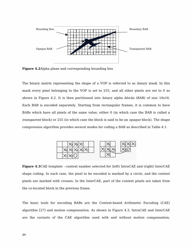
Figure 4.2Alpha plane and corresponding bounding box
The binary matrix representing the shape of a VOP is referred to as binary mask. In this
mask every pixel belonging to the VOP is set to 255, and all other pixels are set to 0 as
shown in Figure 4.2. It is then partitioned into binary alpha blocks (BAB) of size 16x16.
Each BAB is encoded separately. Starting from rectangular frames, it is common to have
BABs which have all pixels of the same value, either 0 (in which case the BAB is called a
transparent block) or 255 (in which case the block is said to be an opaque block). The shape
compression algorithm provides several modes for coding a BAB as described in Table 4.1.
Figure 4.3CAE template : context number selected for (left) IntraCAE and (right) InterCAE
shape coding. In each case, the pixel to be encoded is marked by a circle, and the context
pixels are marked with crosses. In the InterCAE, part of the context pixels are taken from
the co-located block in the previous frame.
The basic tools for encoding BABs are the Context-based Arithmetic Encoding (CAE)
algorithm [27] and motion compensation. As shown in Figure 4.3, IntraCAE and InterCAE
are the variants of the CAE algorithm used with and without motion compensation,
Bounding Box
Opaque BAB
Boundary BAB
Transparent BAB

47
respectively. Each shape coding mode supported by the standard is a combination of these
basic tools.
BAB Type
Type Used in Description
0 No update, without MVD
P-, B-VOP The decoded block is obtained through motion compensation without correction. No motion vector difference is give, i.e. it is set to zero
1 No update, with MVD
P-, B-VOP The decoded block is obtained through motion compensation without correction. A motion vector difference is given.
2 Transparent I-, P-, B-VOP The decoded block is completely transparent. Texture information is not coded for such block either.
3 Opaque I-, P-, B-VOP The decoded block is completely opaque. Texture information needs to be coded.
4 Intra CAE I-, P-, B-VOP The decoded block is obtained through intra CAE decoding.
5 Inter CAE without MVD
P-, B-VOP The decoded block is obtained through inter CAE decoding. No motion vector difference is given i.e. it is set to zero
6 Inter CAE with MVD
P-, B-VOP The decoded block is obtained through inter CAE decoding. A motion vector difference is given.
Table 4.1BAB coding modes (See Figure 4.4 for VOP coding types)
Intra/Inter VOPs Coding
For intra coded VOPs, the BAB types allowed is restricted to 2, 3, and 4 in Table 4.2.1. The
BAB type is encoded using a VLC table indexed by a BAB type context C computed using
Equation (5.1) and IntraCAE template (N=9) in Figure 4.3.
(4.1)
48
where Xk equals 0 for transparent pixels and 1 for opaque. In the case of inter coded VOPs,
all BAB types listed in Table 4.1 are allowed and the BAB type information is encoded using
a different VLC table indexed by context C computed using Equation (4.1) and InterCAE
template (N=8) in Figure 4.3.
BAB motion compensation
Besides the type information, motion information can also be used to encode the BAB data.
In this case the BAB is encoded in intermode and one motion vector for shape (MVs) for
each BAB is used. The motion vectors can be computed by searching for a best match
position (given by the minimum sum of absolute difference). The motion vectors themselves
are differentially coded, which means that for each motion vector a predictor is built from
neighbouring shape motion vector already encoded and the difference between this
predictor and the actual motion vector for shape, MVDs is VLC encoded.
BAB size conversion
The compression ratio of the CAE technique can be increased by allowing the shape to be
encoded in a lossy mode. This can be achieved by encoding a down-sampled version of the
BAB. In this case the BAB can be down-sampled by factor of 2 or 4 before context encoding
and up-sampled by the same factor after context decoding. The relation between the
original and the down-sampled BAB sizes is called conversion ratio. Table 4.2 presents the
different BAB sizes allowed, depending on the value of the conversion ratio parameter.

49
Conversion Ratio BAB size in pixels
1 16 x 16
2 8 x 8
4 4 x 4
Table 4.2List of BAB sizes for CAE
4.3 Motion Coding
Motion coding is used to compress video sequences by exploiting temporal redundancies
between frames and consists of two parts; motion estimation and motion compensation.The
MPEG-4 standard provides three following modes for encoding a VOP as depicted in Figure
4.4.
I-VOP, a VOP may be encoded independently of any other VOP.
P-VOP, a VOP may be predicted using motion compensation based on another
previously decoded VOP.
B-VOP, a VOP may be predicted based on past as well as future VOPs.

50
Figure 4.4The three modes of VOP coding, I-VOPs are coded without any information from
other VOPs. P- and B-VOPs are predicted based on I- or other P-VOPs.
Clearly, the motion estimation is necessary only for coding P- and B-VOPs
andperforms a delta analysis between two consecutive VOPs in question and determines
whether areas of the image have changed or moved between the frames. In many cases an
area stays exactly as it was in the previous frame in case of P-VOP and therefore it is
sufficient for the encoder to inform the decoder to display this area as it was in the previous
frame. If the area moves in a certain direction, the motion estimation algorithm directsthe
decoder to use the same piece of image as inthe previous frame, but to move it a certain
amountin a defined direction. In practice this will be accomplishedby sending motion
vectors within thebit stream. These vectors will guide thedecoder in choosing the
appropriate portions ofthe previously decoded frame to be used in thereconstruction of the
current frame.
As one may expect, the motion estimation is a verycomputationally intensive function.
Searchingthrough an image for all the possible objects (areas)that could change place for
every potentiallocationrequires a lot of calculations.Basically, the MEneeds to take each of
the 16 x 16 MBor 8 x 8 for half-sample precision (or BAB for shape) one at a time and
I-VOP B-VOP P-VOP
TIME

51
'place'it on top of the previous VOP to determine if thereis a match. The matching may be
done by calculatingthe difference between each pixel in the blockand matching the position
in the previous frame.As a result, a number (summation of absolute difference, SAD value)
is obtained whichdenotes whether that particular block fits thatcertain position in the
previous frame. If the SADvalue is zero it means that each of the pixels are inexactly the
same position as in the previous frame and therefore the new position for that block
hasbeen found. If none of the positions match perfectly,the algorithm has two choices:
firstly, it eitherconcludes that all the differences are too greatwhich must mean that the
block in questionis a new entity that did not exist in the previousframe or it has moved too
far from it's previousposition or secondly, in the case of a smaller nonzeroSAD value, it
accepts the best match eventhough this match is not perfect.Typically,the search area is +/-
16 pixels.
As the second part, motion compensation is performed which refers to differential
coding of motion vectors, (x, y) obtained in ME. The motion vector components (horizontal
and vertical) are differentially coded by using a spatial neighbourhood of three motion
vectors already transmitted as shown in Figure 4.5.
Figure 4.5 Motion vector prediction, MVSx is a shape motion vector associated with the
BABx. MVx is a texture motion vector in half-sample precision associated with the 8 x 8
texture block x.

52
The motion vector coding is performed separately on the horizontal and vertical
components. The motion vector predictor candidates, MVPCs are set to the first three
defined motion vector residing in the VOP scanning block on left, above, and right above in
this order. The motion vector predictor is defined as below. If no motion vector is available,
then MVP is set to zero.
The motion vector differences, MVD, given by the following expressions for each
component, are then VLC encoded:
where is the x coordinate for the motion vector and similar for and
The decoder computes the current motion vector in the inverse way using the motion
vectors from the previous decoded MBs and adding the current decoded motion vector
difference, MVD as follows:

53
4.4 Texture Coding
This section merely highlights the main aspects of the texture coding, which are modified
and need further specification when dealing with arbitrarily shaped object.
The texture information of a video object plane is present in the luminance, Y, and two
chrominance components, Cb, Cr, of the video signal. In the case of an I-VOP, the texture
information resides directly in the luminance and chrominance components, In the case of
motion compensated VOPs the texture information represents the residual error remaining
after motion compensation. For encoding the texture information, as described in Section
3.1.2, it follows the same procedure.
The standard 8 x 8 block-based DCT is used. To encode an arbitrarily shaped VOP, an 8 x 8
grid is super-imposed on the VOP as shown in Figure 4.6. Using this grid, 8 x 8 blocks that
are internal to VOP are encoded without modifications. Blocks that straddle the VO are
called boundary blocks, and are treated differently from internal blocks.
Figure 4.6 Texture coding : 8x8 grid is super-imposed (right) on the texture data (left).
Macroblocks that straddle VOP boundaries, boundary macroblocks, contain arbitrarily
shaped texture information. A padding process is used to extend these shapes into
rectangular macroblocks. The luminance component is padded on 16 x 16 basis, while the
chrominance block are padded on 8 x 8 basis. Repetitive padding consists in assigning a

54
value to the pixels of the macroblock that lie outside of the VOP. When the texture data is
the residual error after motion compensation, the blocks are padded with zero values.
The transformed blocks are quantised, and individual coefficient prediction can be
used from neighbouring blocks to further reduce the entropy value of the coefficients as
follows. The DC coefficient of the current 8 x 8 block may be predictively coded. The DC
coefficient is predicted form the DC coefficient in the block directly above it or the block
directly to the let of it.
This is followed by a scanning of the coefficients, to reduce to average run length
between to coded coefficients. Then, the coefficients are encoded by variable length
encoding.
4.5 H.264 and MPEG Standards
A number of standards have been defined for video compression. Table 4.3 summarises the
major ones. H.264 employs the same general approach as MPEG 1 & 2 as well as the H.261
and H.263 standards, but adds many incremental improvements to obtain coding efficiency
improvement of about a factor-of-3. MPEG-2 was optimized with specific focus on Standard
and High Definition digital television services, which are delivered via circuit-switched
head-end networks to dedicated satellite uplinks, cable infrastructure or terrestrial
facilities. MPEG2's ability to cope is being strained as the range of delivery media expands
to include heterogeneous mobile networks, packet-switched IP networks, and multiple
storage formats, and as the variety of services grows to include multimedia messaging,
increased use of HDTV, and others. Thus, a second goal for H.264 was to accommodate a
wider variety of bandwidth requirements, picture formats, and unfriendly network
environments that throw high jitter, packet loss, and bandwidth instability into the mix.

55
H.264 is completely focused on efficient coding of natural video without shape coding and
therefore does not directly address the object-oriented functionality, synthetic video, and
other systems functionality in MPEG-4, which carries a very complex structure of over 50
profiles. MPEG-4 is a family of standards whose overall theme is object-oriented multimedia
applications. It thus has much broader scope than H.264, which is strictly focused on more
efficient and robust video coding. The comparable part of MPEG-4 is Part 2 Visual, called
"Natural Video". Other parts of MPEG address scene composition, object description and
java representation of behaviour, animation of human body and facial movements, audio
and systems.
During 2002, the H.264 Video Coding Experts Group combined forces with MPEG4 experts
to form the Joint Video Team (JVT), so H.264 is being published as MPEG-4 Part 10
(Advanced Video Coding) and will in essence become part of future releases of MPEG-4.

56
Standard Target bit rate
Compression technologies Target application
ISO/IEC MPEG-1
Up to 1.5
Mb/s
-DCT -Perceptual quantization
-Adaptive quantization -Zig-zag reorder
-Predictive MC -Bi-directional MC -1/2 sample accuracy ME
-Huffman coding -Arithmetic coding
-Storage (CD-Rom) -Consumer Video
ISO/IEC MPEG-2
1.5 to 35 Mb/s
-Frame/field-based MC -Spatial scalability
-Temporal scalability
-Quality scalability -Error resilient coding
-Digital TV -Digital HDTV -High quality video -Satellite TV -Cable TV -Terrestrial broadcast
ISO/IEC MPEG-4 (up to part 9)
8 kb/s to
35 Mb/s
-Wavelet -Zero tree reorder -Advanced ME -Overlapping MC -View dependent scalability
-Bitmap shape coding -Sprite coding -Face animation -Dynamic mesh coding
-Internet -Interactive video -Visual editing -Content manipulation -Professional video -2D/3D computer graphics -Mobile
ITU-T H.261
64kb/s to
2Mb/s
-DCT -Adaptive quantization -Zig-zag reorder -Predictive MC
-Integer sample accurary ME -Huffman coding -Error resilient coding
-ISDN video conferencing
ITU-T H.263
8kb/s to 1.5Mb/s
-Bi-direction MC -Advance ME -Arithmetic coding
-1/2 sample accuracy ME -Overlapping MC
-POTS video telephony -Desktop video telephony -Mobile video telephony
ITU-T H.264 /
ISO/IEC MPEG-4 part 10
8kb/s to 1.5Mb/s
-Multi reference MC -1/4 accuracy ME -B frame prediction weighting
-Flexible MB ordering
-Variable size MC -Deblocking filter -4x4 interger transform
-Multi intra prediction - UVLC / CABAC
-Entertainment video -Mobile video streaming -MMS
Table 4.3Summary of present standards for video compression (each standard omits the
same technologies included in its prior standard)

57
58
Chapter 5
Shape Coding
Binary objects form the simplest class of object. They are represented by a sequence of
binary alpha maps, i.e., 2D images where each pixel is either black or white. A shape
represented in a binary alpha plane has the same values for all the pixels that are inside the
shape. As described in Chapter 4, MPEG-4 provides a binary shape only mode for
compressing these objects.
The compression process is defined exclusively by a binary shape encoder for coding the
sequence of alpha maps. However, the compression of arbitrarily shaped object is a major
problem in object-oriented video coding [2B.8,16]. Efficient shape coding schemes are
needed in encoding the shape information of VO in the MPEG-4 standard but also in which
shape coding algorithms is an important problem such as CAD, object recognition and
image description in video databases.
Firstly, we review various intra-frame shape coding technique. The next section details
multiple grid chain code in depth, presents various approaches taken in order to improve
MGCC and experimental results. Following section deals with pre-processing. Hybrid shape
coding is suggested. Finally, inter-frame coding schemes are covered.
5.1 Literature Overview
The problem of region shape representation has been investigated in the past for arbitrary
and constrained regions [28]. The different representations are closely linked to three
major classes of shape representation techniques, namely bitmap, intrinsic and contour-

59
based ones designed only for compression, bitmap-based techniques apply binary image
coding methods, such as those developed for facsimile transmission, to shape images.
Intrinsic shape representation methods either decompose the shape into smaller, simpler
elements (Quadtree-based techniques[33], fractal representation[19], etc), or represent it
by its skeleton. As opposed to the latter region-based methods, contour-based techniques
use a transform to convert the object mask into contours, like in the human visual system.
This representation is desirable in application where a semantic or geometrical description
of the shape is used, such as in database application [29]. In this section, shape coding
schemes exploiting spatial redundancy will be examined.
5.1.1 Bitmap Coding
Bitmap coding techniques operate on the raw data, without performing any prior
transformation. Two such techniques are presented in this section. Both are based on
paradigms that have been successfully applied to black and white image coding, and for
facsimile application in particular. The first one is based on run-length encoding and the
second on arithmetic coding with conditional probabilities.
Modified Modified Read (MMR)
The Modified Modified Read method is based on run-length encoding of a binary image. The
image is scanned line by line and the lengths of each black and each white segment are
encoded. To improve the efficiency of the method the encoding of the length is optimised by
taking into account segment boundaries in the previous line. This algorithm has been
successfully applied in the facsimile group 4 standard. An adaptation of this method to
shape coding is proposed in [30]. Macroblock partitioning is introduced for compatibility

60
with DCT-based texture coding. Furthermore a size conversion procedure is proposed to
achieve lossy shape coding.
Context-Based Arithmetic Encoding (CAE)
As a detailed description of CAE [27] has been introduced Section 4.4, underlying principle
of this scheme will be pointed out. Arithmetic coding [31], mentioned in Section 2.3.2, is a
very efficient entropy coding scheme. Given the probability distribution of symbols in a
string, arithmetic encoding can compress the string to a length close to its entropy. The
standard application of arithmetic encoding to a binary image is as follows. Pixels of the
image are encoded in a predefined scan order, typically raster scan. At each pixel to be
coded, the arithmetic encoder is fed the value of the pixel plus a probability distribution. In
the case of a binary image, this probability distribution reduces to a single number, p0
which gives the probabilities of any pixel being black. The probability of any pixel being
white is simply given by 1-p0.
The efficiency of such a representation depends upon the suitability of the probability
distribution that is used. CAE assumes that a high degree of local correlation exists in the
image. Hence, conditional probabilities are introduced. For a given pixel, the probability
distribution is conditioned upon the values of the pixels in a local neighbourhood. The shape
and size of the neighbourhood is represented by a template as shown in Figure 4.2.2. The
size of the template is typically 10 pixels leading to 1024 different contexts[32]. A context is
an integer specifying the value of each pixel within the template. The context is used to
access a table containing probability distributions. This table is created by a training
procedure prior to coding, or in the case of adaptive CAE, it is adapted during the coding
procedure as in JBIG.
The efficiency of CAE schemes largely depends on the choice of the template. In
general the larger the template, the better the performance. However, the memory for
storage of the probability tables increases exponentially with the size of the template. There

61
is also the risk of over-generalisation when using large templates. In a block-based texture
coding environment, the CAE method can be adapted to proceed in a block-based
fashion[27]
5.1.2 Intrinsic Shape Coding
Intrinsic shape representation considers the region rather than its boundaries. Such
representation methods, also called internal representation methods, were among the first
methods to be investigated in the fields of computer vision and pattern recognition [28]. In
this section, two techniques are presented. They are based on two different approaches to
the problem: the first one consists in representing a shape by its skeleton, and the second
one is a hybrid block/Quadtree decomposition which has been investigated in the
framework of the MPEG-4 video compression standardisation process [34]
Skeleton Decomposition
Skeleton decomposing, also referred to as medial axis transformation (MAT) or symmetric
axis transformation (SAT), has been widely investigated. It consists in describing a full
Figure by its skeleton. Basically the skeleton of a shape can be extracted by taking the
centres of all maximally inscribed disks as shown in Figure 5.1. The shape description
consists of two parts: the symmetric axis or locus of centres of these disk and their
corresponding radius towards the shape boundary. Mathematical morphology operator can
be used to extract the skeleton and corresponding quench values for any pixel-quantised
structural element [35]. Since different structural elements result in different shape
representation, the element used must be either implicitly known by the decoder or
transmitted together with the skeleton and quench values. Shape representation
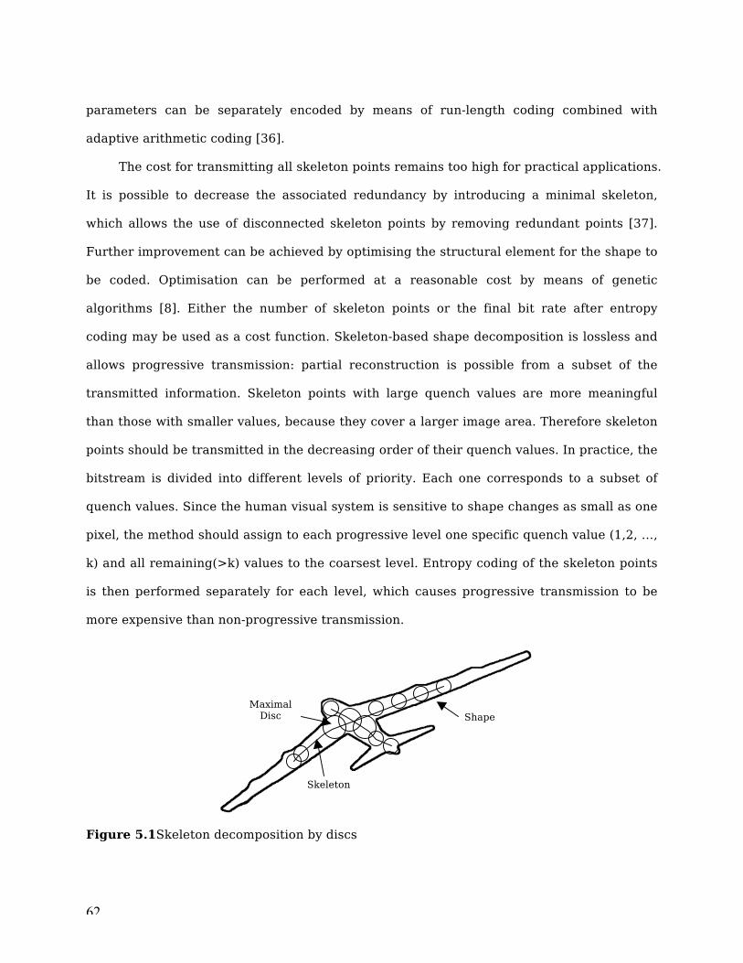
62
parameters can be separately encoded by means of run-length coding combined with
adaptive arithmetic coding [36].
The cost for transmitting all skeleton points remains too high for practical applications.
It is possible to decrease the associated redundancy by introducing a minimal skeleton,
which allows the use of disconnected skeleton points by removing redundant points [37].
Further improvement can be achieved by optimising the structural element for the shape to
be coded. Optimisation can be performed at a reasonable cost by means of genetic
algorithms [8]. Either the number of skeleton points or the final bit rate after entropy
coding may be used as a cost function. Skeleton-based shape decomposition is lossless and
allows progressive transmission: partial reconstruction is possible from a subset of the
transmitted information. Skeleton points with large quench values are more meaningful
than those with smaller values, because they cover a larger image area. Therefore skeleton
points should be transmitted in the decreasing order of their quench values. In practice, the
bitstream is divided into different levels of priority. Each one corresponds to a subset of
quench values. Since the human visual system is sensitive to shape changes as small as one
pixel, the method should assign to each progressive level one specific quench value (1,2, …,
k) and all remaining(>k) values to the coarsest level. Entropy coding of the skeleton points
is then performed separately for each level, which causes progressive transmission to be
more expensive than non-progressive transmission.
Figure 5.1Skeleton decomposition by discs
Shape Maximal
Disc
Skeleton

63
Hybrid Macroblock / Quadtree for Binary Shape Representation
The shape coding method described in [34] is based on a 16 x 16 pixel macroblock partition
to facilitate its integration in existing block-based video coding schemes. A block is said to
be uniform inside if all the pixels in it belong to the region being coded and uniform outside
if all do not. These blocks are simply indicated to decoder through a simple flag. Each non-
uniform block is further recursively split into four square subblocks as illustrated in Figure
5.2 The resulting block hierarchy is represented in a Quadtree. Uniform outside and
uniform inside subblocks are tagged as leaves, while non-uniform subblocks are further
split. The resulting combination of outside leaves, inside leave and split subblock are
described by indices that are entropy coded with Huffman code. In addition, index
swapping procedures have been introduces to increase coding efficiency [34].
Although this technique is intrinsically lossless, filtering the shape before coding can
increase compression performance and facilitate rate control. A pre-processing stage is
applied to increase the proportion of large uniform block which require less bits for coding.
One drawback of this approach is the introduction of blocking artefacts along the shape
contours. However, these may be reduced by appropriate post-filtering.
Figure 5.2Hybrid macroblock / Quadtree structure

64
5.1.3 Contour-Based Coding
A region may also be represented by their contours. In chain code algorithms, the contour
of a region is connected chain of pixels. On the other hands, methods such as polygonal
approximation and higher order approximation make use ofgeometrical representation.
5.1.3.1 Chain Coding
In this section, we discuss methods for representing contours by chains of adjacent
boundary pixels. Both lossless and lossy representations are discussed.
5.1.3.1.1 Lossless Coding
Freeman’s chain code [38] may be used to represent contours of regions efficiently. Chain
coding is based on the observation that the relative positions of any two adjacent points on
a line in a digital images, are restricted to on of eight configurations (four possible
configurations if 4-connectivity is considered) as shown in Figure 5.3. Thus, from a given
point on the line, the transition to the next point can occur in one of eight directions. Each
transition from one point to the next is called a link. The chain code for a line is formed by a
sequence of links. The chain code representation of a contour is constructed as follows.
Firstly, select a staring point on the contour. Represent this point by its absolute
coordinates in the image. Secondly, represent every consecutive point by a link showing the
transition needed to go from the current point to the next point on the contour. Lastly, stop
if the next point is the initial point, or the end of an open contour. In the case of open
contours, either a special and symbol may be encoded or the total number of chain symbols
may be transmitted prior to symbols.

65
Such a chain code is referred to as Freeman code. Since every pixel in the contour is
represented in the chain code, this method is lossless for encoding contours. Below, we
discuss the basic Freeman code and some other schemes derived from it.
Figure 5.3Contour representation and 8-connectivity chain, 4-connectivity chain
Freeman Codes
Freeman codes have been widely accepted as the preferred method for representing
contours, as they are highly efficient compared to the naïve representation where each
point on the contour is represented by a pair of absolute coordinates. Since a link in a
Freeman code represents one of only eight possible directions, a set of eight symbols is
sufficient to represent a Freeman-coded contour. Each of the eight directions may be
represented by a string of 3 bits. Thus, the contour may be encoded in binary bit-string with
3 bits/link.
The above Freeman coding scheme is based on the 8-connectivity of contour points.
Alternatively, we may choose to represent a contour using 4-connectivity, where only
transitions in four directions are allowed. Thus, a set of four symbols is sufficient to
represent contours based on 4-connectivity. This results in a Freeman code costing only 2
bits per link. Ostensibly, this gives us an improvement of 33% longer than the
corresponding 8 –connected chain[39]. In fact, 4-connected chains are not efficient to

66
represent diagonal moves, requiring two link where 8-connected chains only us one link. As
the geometric resolution of the image increases, 8-connectivity becomes more and more
efficient compared to 4-connectivity. Hence, 4-connectivity is not commonly used for
constructing Freeman codes for contours.
Differential Codes
Differential chain codes, also proposed by Freeman [40], can offer substantial improvement
in encoding efficiency, compared to Freeman codes, Our discussion of differential chain
codes is based on 8-connectivity. The differential chain code representation for a contour
may be constructed based on its Freeman code. Here, each link is replaced by its difference
from the preceding link. Mathematically the Freeman code C of a contour may be
considered as an ordered-set of links.
(5.1)
where linkirepresent the i th link in the chain of length N. let , for
We can define
(5.2)
where di is the i th link in the differential chain code.
Entropy coding may be applied to encode differential chain codes efficiently. The number of
symbols required to represent a differentially coded chain is the same as that required for
the corresponding Freeman code. However, unlike in the case of Freeman coding, the
distribution of the symbols in the differential chain code is not uniform. We can expect the
directions represented by two consecutive links in the Freeman code to be similar.

67
Therefore the difference between the links is generally small. For images with sufficiently
fine resolution, most links in the differential chain code have values of -1,0, or 1. A suitable
entropy -based encoding scheme may be developed to exploit this knowledge. A simple
Huffman coding scheme can be used, associating a variable length code to the different
possible symbols. The most likely differential values, 0, will be assigned a single bit code
word and so on [41]. In general, a rate of about 2bits per link may be expected, using
Huffman encoding of differential chain coded contours.
Improved Entropy Coding
Several attempts to improve the efficiency of differential chain codes have been reported in
the relevant literature. These methods usually relay on specific knowledge about the
characteristics of the contours or lines in question, in order to establish tighter upper-
bound on the entropy of the corresponding differential chain codes. This leads to improved
efficiency in entropy-based encoding.
Kaneko and Okudaira [42] proposed an algorithm for coding smooth contours, in
which the contour is first divided in to a sequence of segments. Within a segment, each link
must be in one of two adjacent directions, thus only requiring one bit per link. The length
and the dominant direction of the segment must also be transmitted. The smoother the
contour, the longer the segments, and hence the higher the encoding efficiency. For the
case of rough contours, the average length of each segment is small. In such cases this
method offers about the same efficiency as the differential code.
Eden and Kocher [43] have proposed an encoding scheme in the context of 4-
connected Freeman coded contours. Their method is based on a first-order analysis of 4-
connected contours. They introduce three symbols to represent different combinations of
pairs of adjacent links: left, right, and ahead. These three symbols deal with representing
the 4-connected contour. The resulting entropy for a contour with N points is .

68
Note that, except the case of very short contours, a right turn I never followed immediately
by another right turn. The same can be said for left turns. Using the constraint that
consecutive turns of the same type should never occur, Eden and Kocher reduce the bit rate
per link from down to .
Lu and Dunham [44] used Markov models to describe the structure of the chains. The
differential chain code is considered as a Markov source, and is encoded using an entropy -
based encoding scheme. The transition probabilities related to the chosen Markov model
are computed experimentally. These probability values are used to construct appropriate
entropy -based encoder. Using a Huffman encoding scheme based on a second order
Markov process, they achieve encoding rates similar to those obtained using the method of
Kaneko and Okudaira, described above. However, the Markov model-based scheme is
simpler to implement. They show that significantly better encoding rates can be obtained by
using an arithmetic encoding scheme [31]based on a second order Markov model. On
average, this method performs about 25% better than the simple Huffman encoding scheme
for differential chain codes.However, the additional cost of storing, and eventually
maintaining, the transition tables must be taken into account.
The schemes mentioned above are restricted within lossless compression that is not
flexible to allow the control of shape bit rate. The flexible bit rate control capability is
essential in communication where channel capacity is variable. (See Chapter 6 for details).
5.1.3.1.2 Lossy Schemes
The chain coding methods discussed in the previous section are lossless, as the encoded
contour can be reconstructed exactly. At the expense of accuracy, some encoding efficiency
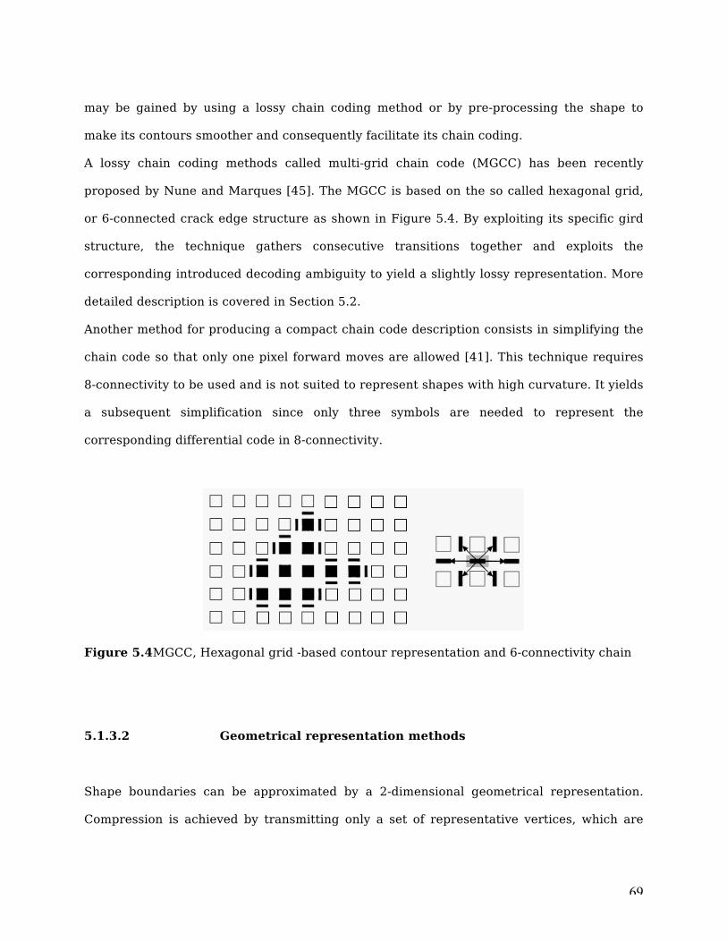
69
may be gained by using a lossy chain coding method or by pre-processing the shape to
make its contours smoother and consequently facilitate its chain coding.
A lossy chain coding methods called multi-grid chain code (MGCC) has been recently
proposed by Nune and Marques [45]. The MGCC is based on the so called hexagonal grid,
or 6-connected crack edge structure as shown in Figure 5.4. By exploiting its specific gird
structure, the technique gathers consecutive transitions together and exploits the
corresponding introduced decoding ambiguity to yield a slightly lossy representation. More
detailed description is covered in Section 5.2.
Another method for producing a compact chain code description consists in simplifying the
chain code so that only one pixel forward moves are allowed [41]. This technique requires
8-connectivity to be used and is not suited to represent shapes with high curvature. It yields
a subsequent simplification since only three symbols are needed to represent the
corresponding differential code in 8-connectivity.
Figure 5.4MGCC, Hexagonal grid -based contour representation and 6-connectivity chain
5.1.3.2 Geometrical representation methods
Shape boundaries can be approximated by a 2-dimensional geometrical representation.
Compression is achieved by transmitting only a set of representative vertices, which are

70
then used to reconstruct the contour via line or spline segments. Geometrical
approximation methods are usually lossy, and allow simple distortion control by
constraining the geometrical representation accuracy to a maximum allowed error. Several
geometrical representation methods exist based in different vertex selection, curve
reconstruction and entropy coding approaches. Whereas entropy coding constitutes a
relatively independent problem, vertex selection and curve reconstruction are closely
linked, vertices being optimally selected with regard to a specific geometrical
reconstruction model.
Figure 5.5 Polygonal approximation
5.1.3.2.1 Polygonal Approximation
Polygonal approximation is the simplest geometrical approximation, where only the
positions of the vertices need to be encoded as depicted in Figure 5.5. Since digital images
are sampled on a finite grid, a lossless representation can be achieved for any shape,
corresponding to the removal of intermediate contour pixels in contour straight lines: in the
worst case where no straight lines exist in the shape boundaries, all contour pixels are
polygon vertices. The polygonal approximation encoding process consists of contour

71
extraction, vertex selection and vertex coding. The decoding process requires vertex
decoding followed by a polygon filling procedure [46].
In the context of data compression, the polygonal approximation which has the least
number of vertices, and which confirms to a predefined error criterion, is generally
considered as the optimum. Different error criteria may be used to measure the
approximation quality [47]. A simple, sub-optimal, vertex selection algorithm based on
interactive refinement was originally proposed in [48]. The first approximation is
recursively refined by inserting a new vertex on the contour point which is furthest away
from the current approximation. This vertex insertion procedure stops when the distance
between the approximated contour and any contour pixel is smaller than a given threshold
as illustrated in Figure 6.1.3.1. More sophisticated algorithms, which do not only split but
also merge segments, have been developed [49]. A review of polygonal approximation
methods is given in [50].
Efficient schemes encode only the position of the first vertex in absolute coordinates.
The subsequent vertices are differentially coded, relative to the previous vertex. To actually
improve compression, entropy coding is used. When the maximum allowed error is large,
only a few vertices are needed. Their positions are usually not highly correlated, and
entropy coding does not improve compression performance. When the maximum error is
small, the vertices are numerous, and close to their neighbours. Entropy coding then
becomes more efficient. In the limit, when the error is set to zero, polygonal approximation
becomes very much like chain coding, and corresponding entropy coding schemes may be
used.
5.1.3.2.2 Higher Order Approximations

72
A higher order geometrical representation can be provided by cubic curve interpolation. To
reconstruct the approximated curve between two vertices, two constraints, such as
derivatives or control points, are considered in addition to the coordinates of each endpoint.
The resulting approximation is smoother and is visually more pleasing. However, it is not
well suited to represent sharp angles.
Higher Order Approximation Schemes
A contour coding method based on approximation by blending curves was proposed in [51]
to achieve rate-distortion optimization for a region-based coding scheme. The number of
vertices is constrained by the available rate budget. Vertex positions are calculated in order
to minimize the approximation distortion. Any distortion measure may be used. A popular
one is the maximum local error defined as the distance between the original contour and
the spline. Initially, the corresponding vertices are equidistantly distributed along the
contour to be approximated. A steepest descent optimisation technique, consisting in
successively perturbing each vertex along the eight possible directions, is then applied. For
each possible move, the four splines affected by the perturbed vertex are updated, and the
corresponding error is computed. The position minimizing this error is retained. The
algorithm is iterated until the error drops below a predefined threshold.
The algorithm minimises the error for only one vertex at a time and the final solution
is generally suboptimal. Moreover, whereas the algorithm requires a predefined number of
vertices, no method is proposed to adapt the number of vertices to shape features. In [51]
the contour optimization is carried out for different numbers of vertices and the solution
minimizing the rate-distortion criterion is chosen (rate and distortion being defined in that
case with regards to the whole region-based coding scheme, not only the shape coding
module).

73
Another method uses Hermite curves [46] to approximate the contours [52]. At each
vertex the tangent of the reconstructed curve is constrained by the tangent of the original
contour. Vertices are recursively selected according to a scheme similar to the ones used
for polygonal approximation. As opposed to the former method that constrains the rate, this
method constrains the distortion.
Hybrid Polygonal/ Cubic Curve Representation
Polygonal approximation is not suitable for smooth shapes, whereas cubic curve
approximation cannot represent sharp edges. Therefore, a hybrid polygonal/cubic curve
approximation is expected to be more efficient [53]. Basically, two approaches are possible:
either the polygon/curve switch and the encoding of the corresponding one bit flag are done
at vertex level, or at region level, relying on the assumption that object shapes are likely to
be best described either by smooth curves only or distinct angles only, not by a combination
of the two. With regard to the curve or polygon only approximations, the latter scheme
requires only one additional bit for each region while exploiting the advantages of both
techniques. Moreover, both schemes require the implementation of a decision scheme,
either at a global or at a local level. In practice, both approximations are considered and
the better one is used. However, this raises dependency problems when a local switch is to
be applied, since spline and polygonal approximation methods do not share the same vertex
selection procedure.
5.2 Multiple Grid Chain Coding

74
In this section, we will identifydeficiency of the shape coding method developed by Nunes
and Marques, i.e. Multiple Grid Chain Code (MGCC) [45] and attempt for improvement. The
technique is an essentially lossy compression scheme.However,visual losses are hardly
noticeable to the Human Visual System. A 3 x 3 cell structure offers an efficient contour
representation by simplification and prediction of contours while inter-relation between
cells can be further optimised with anisotropy and directionality. We will review overall
MGCC scheme and then, consider various approaches for improvement of the
scheme.Author like to state that a lossless approach using 2 x 3 cell(Section 5.2.2.3)iswill
be presented inEUSIPCO 2005
5.2.1 Quasi-Lossless Shape Coding
The scheme offers a highly efficient quasi-lossless contour-based coding. As introduced in
the Section 5.1.3.1.2, the MGCC utilizes the hexagonal grid where the boundary of a shape
is represented by edge sites located between two adjacent pixels as shown in Figure 5.4.
The scheme uses a square cell of an area of 3 x 3 pixels of the hexagonal grid as depicted in
Figure 5.6.
Figure 5.6 Type of MGCC cells: (left) clockwise (right) counter-clockwise
Any path starting from the entry, denoted 0, to the exits within cell can be encoded by the
exits {1,2,…, 7}. This is where the contour simplification is used which allows reducing bit

75
rate. However, this introduces ambiguities in decoding process as certain exits can
corresponds to more than one contour configurations as shown in Figure 5.7, thereby
contour is predicted before encoding by means of cell type selection.
Figure 5.7Ambiguities introduced by MGCC
The MGCC maintains another horizontally flipped cell in order to improve the prediction of
contour. In other words, following contour is predicted based on the current contour and
the type of the subsequent cell, Celltype(n+1), which would encode the contour efficiently, is
chosen accordingly using a function below.
(5.3)
where function Select is defined as follows
(5.4)
where implies the other type of cell
The scheme keeps the track of the absolute direction that the last edge of cell is pointing in
order to apply the subsequent cell relative to the direction. Figure 5.8 is an illustration of
the coding example where coding progresses from the top left cell. The description of the
used cells is given in Table 5.1. As objects are in closed, a termination of encoding process
is determined when aninitialedge is reached back.Then, resulted chain symbols (exits) are
Huffman coded. (See Appendix for codewords)

76
Figure 5.8Example of the MGCC coding scheme (number denotes exit taken)

77
Table 5.1 Description of cells in Figure 5.8
5.2.2 Improvement
This section describes the attempted approaches to improve the MGCC scheme. The first
sub-section presents an attempt to improve efficiency within a cell, utilising the structure of
a cell. The second part addresses an attempt combining polygonal shape coding and chain
code. The third approach discusses employing two new properties, the directionality and
the anisotropy, which improved bit rate efficiency by 20% at most.The next
approachdiscusses flexible directionality. Finally,last section covers the evaluation of all
approaches above.
5.2.2.1 Approach 1 : Efficient Cell
The first approach taken was maximising the coding efficiency of the MGCC cell itself. A
vertex is assigned between every two consecutive edges in the existing cell except the four
corners as shown in Figure 5.9. Any contour can be configured using three basic
movements (straight ahead, right turn, and left turn) as depicted in Figure 5.9 (right) in a
similar way to the differential code described previously in Section 5.1.3.1.1. This requires
three distinguishable codewords to represent the basic movements. However, this process
can be simplified using a diagonally halved cell utilising the vertex -based structure.

78
Figure 5.9Vertex -based cell:(left) vertex -based MGCC cell, (right) basic movement which
can describe any shape of contour (ahead, right, left).
Figure 5.10Diagonally halved cell (left) diagonally halved cell: basic movement (bold) at
left bottom, (right) illustrateencoding procedure.
The square cell is halved diagonally as depicted in Figure 5.10. Therefore, the basic
movements are reduced to two, which can be found in the left bottom corner of the halved
cell. The basic movements can be extended as follows in order to encode contours. From
level A to C choose either 0 or 1 at each level to match the contour i.e. with the contour
shown in a square cell in Figure 5.9 (left) can be coded by 1 at level A and 0 at level B.
Hence, cells encode contour at a rate ofmost 3 bits per cell, which is similar bit rate as
MGCC (see Appendix for codewords) while perfect reconstruction is achievable.
However, the consideration above is limited within cell. Problems arise when cells are
connected each other. For every two consecutive cells, it needs additional bits indicating
flipping of cell and the direction of next cell also must be sent to the decoder when next cell

79
is flipped. Besides, a codeword for this indication must be distinguishable from any other
codewords. This approach is only focused on cell efficiency without consideration of
overhead it requires with respect to inter-cell relation.
Note that the MGCC cell, locally, is an optimized contour representation tool for flexible
movements with negligible losses by encoding the final edge relative to the previous cell
and predicting intermediate edges. With respect to the manner that exits of cell represent
movements, the hexagonal grid also offers basis for non-redundant description of contour.
5.2.2.2 Approach 2 : Polygon Based Chain Coding
In the second approach, we concentrated on the efficiency of structure between cells. As
shown in Figure 5.11, the shape is approximated using polygon, and then chain coding is
applied between two consecutive vertices.
(a) (b) (c)
(d) (e) (f)

80
Figure 5.11Polygonal Approximation and Chain codes: (a)source binary image, (b)vertices
are marked in red dot on (a), (c)the contour shape is approximated by polygonal edge,
(d)red box in (c) is magnified, (e)MGCC is applied on the(d), (f)depicts cells used in
(e)(only exits on cell boundary ‘C’ and ’D’ are used).
There is a point to stress from the approach that combining chain code with polygonal
approximation. With careful look at cells that used in two consecutive vertices, for example
in Figure 5.11(e),(f),we notice that only exits residing at the right(D) and the
bottom(C)boundary are used while the rest of exits requires no codeword. We can usethe
codewords for those exits on further defining specific movements instead toward bottom
and right border, which reduces ambiguity in decodingprocess. Under this strategy, two
kinds of simplified cell are devised as depicted in the Figure 5.12. It is obvious that this new
scheme can encode contour with less distortion as path information is encoded, however it
is yet redundant to encode the same contour data twice by polygon approximation and
byMGCC. Instead of polygonal vertex, a MGCC cell that connectsthe simplified cells
smoothly can be substituted.
Figure 5.12 Simplified cells required for polygon -based chain coding
Again we encounter the same problem as one in the previousapproach. We need additional
bitsindicating change between two cell types, the ordinary MGCC cell and the simplified
MGCC cell. It is not clear if overall performance can be enhanced with theoverhead
information.

81
5.2.2.3 Approach 3 : Directionality and Anisotropy
Previously, we have looked at the coherence of type of cell between successive vertices. The
approach exploiting such coherence was limited by the hidden overhead. In this section, we
attempt to find strong coherence of every successive cell in general aspect. We first revisit
the MGCC and analyse the inter-cell relation before further attempts.
For MGCC scheme, globally, the correlation between consecutive cells is reflected in the
scheme less-effectively. Simply, the selection rule and types of cell are devised to place the
subsequent cell on which it would embrace as many contour edges as possible, resulting the
higher efficiency. However, as only two types of cell are available, the selected cell is
inevitably not always optimal. On the other hand, the coding based on the two types
provides robustness in coding sense. In most case, either of types will not be ideal, but will
be tolerable at a certain extent and offer reasonable efficiency. The issue is the
directionality concerning which direction the subsequent cell should be placed in to encode
more edges. Intuitively, there exists trade-off between the robust coding by less
directionality and reliable selection ruleand the efficient coding by flexible directionality
and less reliable selection rule. In order to keep both characteristics, a selection rules are
required to better predict adequate directional cell type for following contour. Under
reliable selection rules, the emphasis on the directionality with the square cell might be
pointless as it barely changes order of exits. Hence, we propose a scheme thatcell to cell
relation is captured effectively into selection rules and cell efficiency is enhanced by
employing the directionality and the anisotropy.
Directionality
As mentioned, the conventional scheme offers two types of cell which generally leads to the
robust coding to a wide range of contour variation. The idea of the new scheme is
increasing coding efficient by the directionality while the robustness is maintained by the

82
reliable selection rules. The strategy assumes that a cell facing a direction always offers
efficient representations for movements in the direction ({4, 5}) mainly and its
neighbouring direction ({2, 3}). We can apply new idea on existing cells encoding a smooth
curve in Figure 5.8. Instead of rotating the current cell for subsequent contour, the
directional information and the type of the cells are kept consistent as those of the first cell
for all the cells shown. Then, the entry position of each cell is changed accordingly. This
produces that all the exits are among likely exits, {2, 3, 4, 5}. The additional entry is
introduced on the same corner of the cell (exit={7}). Of course, the both entries ({0,7})
cannot be present simultaneously in the same cell. This creates extra cell types depending
on where the entry is for each type of the cell. Therefore, four type of cell is available. We
define a term fragment for such contour which can be encoded by only likely exits and by a
single cell type. Encoding the fragment can be expressed as direction of the first cell exit
and a sequence of likely exits as below.
(5.5)
An object can be decomposed into a sequence of fragments. The dynamic cell type change
is applied between fragments. Obviously, the unlikely exit ({1,6,7}) means that the
beginning of another fragment at the subsequent cell and the directional information should
be updated accordingly. In sum, the directionality involves additional entry on the side of a
cell and produces two additional cell types. Each cell type is pointing at four different
directions. Yet, it is too early to mention efficiency by the directionality. Besides,
appropriate selection rules should be provided to apply adequate type at right time.
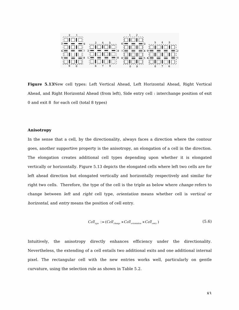
83
Figure 5.13New cell types: Left Vertical Ahead, Left Horizontal Ahead, Right Vertical
Ahead, and Right Horizontal Ahead (from left), Side entry cell : interchange position of exit
0 and exit 8 for each cell (total 8 types)
Anisotropy
In the sense that a cell, by the directionality, always faces a direction where the contour
goes, another supportive property is the anisotropy, an elongation of a cell in the direction.
The elongation creates additional cell types depending upon whether it is elongated
vertically or horizontally. Figure 5.13 depicts the elongated cells where left two cells are for
left ahead direction but elongated vertically and horizontally respectively and similar for
right two cells. Therefore, the type of the cell is the triple as below where change refers to
change between left and right cell type, orientation means whether cell is vertical or
horizontal, and entry means the position of cell entry.
(5.6)
Intuitively, the anisotropy directly enhances efficiency under the directionality.
Nevertheless, the extending of a cell entails two additional exits and one additional internal
pixel. The rectangular cell with the new entries works well, particularly on gentle
curvature, using the selection rule as shown in Table 5.2.

84
Table 5.2 Selection rules: determine subsequent cell type (where Change column indicates
change left cell type to right cell type or vice versa and change of directional information).
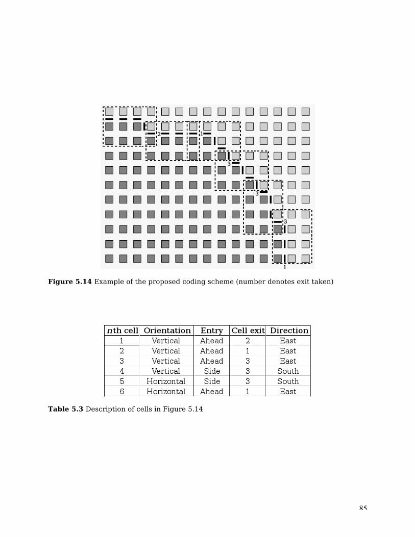
85
Figure 5.14 Example of the proposed coding scheme (number denotes exit taken)
Table 5.3 Description of cells in Figure 5.14

86
Figure 5.14 briefly depicts the coding process based on the both properties on the same
contour as Figure 5.8. However, the additional internal pixel causes worse mismatches of
decoded paths and actual contour configurations as depicted in Figure 5.15. This issue will
be discussed in the Section 5.2.2.5 Evaluation
Figure 5.15Further ambiguity introduced by elongation.
To summarise, the new approach is based on the interaction of the both properties and
theoretically it offers further enhanced bit rate by the improved efficiency at the level of cell
to cell relation using flexible direction and adaptability to contour by reliable selection rules
and elongating cells. Also, the complexity of computation remains same as O(n) where n is
the number of edges wrapping object. On the other hand, the provision for more distortions
by further ambiguities exists.
5.2.2.4 Approach 4 : Flexible Directionality
In the fourth approach, we attempted to improve the directionality which was limited to
either horizontal or vertical by introducing a diagonal direction as shown in Figure 5.16. As
mentioned in the previous section, more directionality may increase coding efficiency under
a reliable cell selection rules.

87
Figure 5.16Diagonal direction
However, introducing additional direction to the existing scheme without much overhead is
not a trivial task because not only a diagonally-directed cell as depicted in Figure 5.17 has
more exits requiring longer codewords, but also it is rather risky and ambiguous to predict
subsequent contour by choose one among three cell types; vertical, horizontal and diagonal.
Figure 5.17Diagonally-directed cells
Therefore, new strategy is adopted as follows. As opposed to the existing scheme encoding
contours within a cell by storing the exit edge and predicting intermediate edges,
intermediate edges are encoded and entry and exit are predicted. We use 2 x 3 cell as a
basic structure as shown in Figure 5.18. There exist only one intermediate edge and three
possible entries and exits respectively.

88
Figure 5.182x3 cell as a basic structure (entry: light shaded edges, intermediate: block
edge, exit: dark shaded edge)
Thirteen 2 x 3 cells including the initial cell are composed together to create a template as
shown in Figure 5.19. Hence, there are twelve possible outputs representing a cell that
contour ends. The template is applied in the same way as the MGCC cell is used to encode
contour, but without selection rules as there is only one template.
Figure 5.19Template composed of thirteen 2 x 3 cells: (left) layout of 2x3 cells (right)
template where black edge represent an intermediate edge for each cell.

89
Figure 5.20Coding Scheme Screenshot : (from left) MGCC (red: counter-clockwise type,
blue: clockwise type), NEW1(yellow: right type, red: left type), NEW2 (same as NEW1),
LOSSLESS 2X3, NEW3
5.2.2.5 Evaluation
For the purpose of evaluation, the MGCC scheme and the proposed schemes were examined
on efficiency with respect to bit rate and distortion rate by coding CIF format binary
segmented image sequence (300 frames) including ‘Children’, ‘Weather’ and ‘Stefan’. The
distortion, Dn is measured for each frame as below. Figure 5.20 presents screenshots of
coding schemes.
(5.7)

90
(i) Approach 3 (NEW1): The proposed approach based on the directionality and the
anisotropy outperformed the conventional scheme in terms of bit rate as shown in Table
5.4. Compared with Freeman’s chain code, it is more than 50% gain. However, the
distortion rate increased though losses are still negligible. The rise of the distortion rate is
mostly due to further ambiguities brought in by the anisotropy property as mentioned
earlier. Intuitively, the fewer bits are used for compression, the more distortions are
resulted in decoder side. Therefore, further evaluation is required. (See Appendix for
codewords)
Table 5.4Experimental results: average for 300 frames for each sequence of CIF format.
(where value in percentage in bracket indicates gain over MGCC, i.e. (12%) )
(ii) Approach 3 with less distortion (NEW2): To inspect whether the gains outweigh the
losses, further analyses were conducted. For every frame of the sequence, the distortion
rate was examined with respect to the number of each exit. Based on the statistical result,
particular movements turning to the side direction (i.e. exit 3, 4 and 5) were less involved in
Weather than in the other sequences. It was discovered that statistically the more those

91
exits are used, the higher distortion rate is as the distortion rate result on Weather is as low
as that of the MGCC in Table 5.4
To reduce the distortion rate, the movements to exit 3 and 4 were further specified
depending upon their paths within the cell and additional chain code symbols were assigned
to each path as shown in Figure 5.21. As a result, the distortion rate dropped off below that
of the MGCC in most frames of all sequences while still 5-16% of bit saving was achieved as
shown in the third row (NEW2) of Table 5.4. (See Appendix for codewords)
Figure 5.21Auxiliary codewords are defined for above each specific movement in order to
improve the quality of reconstruction (from left to right , top to bottom, each movement is
denoted as 4,4a,3b,3,3a) Note that any movement to exit4 is regarded as 4 except for 4a,
similarly any movement to exit3 is regarded as 3 except for 3a,3b.
(iii)Approach 3 using 2 x 3 cell(LOSSLESS 2X3): With the successful result by the previous
approaches, the same scheme based on 2 x 3 cell is tested. Figure 5.22 shows 2 x 3 cells
and Table 5.5 presents the selection rules adapted to 2 x 3 cell structure. As 2 x 3 cell has
only one intermediate edge, compression is lossless. As shown in Table 5.4, the result of
this approach outperforms the MGCC lossless scheme in all test sequence. In particular, in

92
Weather sequence, the bit rate of this lossless scheme is even lower than that of MGCC
lossy compression (See Appendix for codewords)
Figure 5.222 x 3 cell types: (from left) Left Horizontal Ahead, Left Vertical Ahead, Right
Vertical Ahead, and Right Horizontal Ahead (Side entry cell : interchange position of exit 0
and exit 5 for each cell (total 8 types))
Table 5.5 Selection rules adapted for 2 x 3 cell structure

93
(iv)Approach 4(NEW3) : In this approach, in order to provide more flexible directionality
new strategy to encode contour is attempted which intermediate edge is determined and
entry and exit are predicted. Only one kind of template is used so no selection rule to
predict subsequent contour is required. As one might expect, higher coding efficiency was
achieved than the previous approach as shown in Table 5.4, however distortion rate is
relatively high compared with the distortion rate of the previous approach. This is due to
more contour mismatches during determining exit of the initial cell and entry of the final
cell when decoded. (See Appendix for codewords)
(v)Conclusion:It was concluded that, for approach 3, the reduction of bit rate outweighs any
additional losses introduced. Yet the overall distortion of the initial approach is still
negligible. The efficiency of the proposed scheme in terms of bit rate and distortion rate
was dependent on roughness of contour (the smoother contour is, the more predictable by
selection rules) but higher efficiency was achieved over the conventional scheme in all of
the test sequences. However, there is a limit on flexibility of the directionality by this
approach as more directed cell type will cost additional bit rate for indicating change of cell
type, even with selection rule there is risk of contour mismatch resulting increase in
distortion rate.
One template emphasizing directionality can increase bit rate as there are more directions
to represent by codewords. Attempt to reduce the increased bit rates by contour prediction
and simplification increase distortion rate. Therefore, it is important to find a good average
rate between degree of directionality and bit rate. Similar discussion can be made with the
anisotropy. Figure 5.23 presents reconstructed contour shape for approaches above.

94
Figure 5.23 Contour reconstruction of 10th frame of children sequence: (from left) original,
reconstruction by MGCC, NEW1, NEW2, NEW3
5.2.3 Pre-Processing
One way to improve the performance of chain coding schemes without adapting the
corresponding algorithms consists in pre-processing the shape.Rough contour with abrupt
curvature, also regarded as noise generated in object segmentation, is indeed expensive to
encode as such contour is difficult to predict by the selection rules.Figure 5.24 is a brief
illustration of pre-processing procedure.
Contrarily, smooth contours are indeed cheaper to encode. Moreover, a pre-filtering step is
particularly relevant for noisy masks obtained from an imperfect former segmentation stage.
Various filters may be used, such as a median filter, a morphological open-close-close-open
filter, or the majority filter introduced in [54].
A shape coding scheme titled ‘Modified Differential Chain Code (MDCC)’ is developed by
Graham and Chen [55]. The underlying principle of the scheme is to replace unusual
contour with usual one so as to increase occurrence of corresponding chain codes, hence

95
reduces length of codeword and increases coding efficiency. Such contour substitution
mechanism is melded into the differential chain coding. According to their experimental
result, it outperforms differential chain coding with very low distortions but does not
MGCC. However, the scheme is very effective in smoothing the expensive coding contour
without affecting the way the reconstructed contour is perceived by human visual system.
The scheme can be substituted into any coder described above as a pre-processing
procedure filtering out noise. Besides, the improved MGCC coding was based on
exploitation of contour coherence. Therefore, the greater coherence by the pre-processing
will enhance coding efficiency further.
Figure 5.24 Illustration of pre-processing

96
5.3 Hybrid Coding
Previously we discussed the contour-based shape coding technique, multiple grid chain
coding in particular. The method utilising the hexagonal grid encodes the simplified
contours using 3 x 3 cell structure. Its variant employing the directionality and the
anisotropy achieves higher efficiency with the even lower distortion. However,
fundamentally, the efficiency of such technique is limited by the trade-off between a degree
of directionality and the distortion rate even though its is highly efficient. For example, the
more flexible direction is provided, the less unreliably the next cell type is predicted by the
selection rules, hence results the more distortion.
In this section, we attempts to adopt new algorithm, so called Radon transform in order to
approach the shape coding at different angle. Radon transform is a very compact line
representation of which any shape contour is decomposed. In fact, lines constituting a
shape have variable lengths and orientations whichQuadtree structure may be utilised to
represent.
A hybrid shape coding by Radon transform and Quadtree structure is examined and then,
we propose another hybrid scheme based on chain coding and Quadtree structure.
5.3.1 Radon Transform / Quadtree Hybrid Coding
As mentioned, shape can be decomposed into a variable length of lines rotated by angles up
to 180 degree. Quadtree structure provides variable size of block which facilitates variable
length of line while Radon transform can represent a line with various angles. In this
section we seek a way to encode contour using such transform and a variant of the
structure introduced in Section 5.1.2.2.

97
Radon Transform
The transforms are able to transform two dimensional images with lines into a domain of
possible line parameters, where each line in the image will give a peak positioned at the
corresponding line parameters. Firstly, let us take a look at a compact line representation.
Figure 5.25Radon transform (left) binary image with line (right) Radon transformed image
where peak is coloured as red.
There exist several forms expressing lines. A most common form expresses lines in the form
as below.
(5.8)
where is gradient of the line and is distance from the x-axis. However, this simple form
has disadvantage when a line becomes vertical as the gradient parameter, increase
exponentially. Hence, the expression is not suitable for a compact line representation. The
alternative line expression is as follows.
(5.9)

98
where is the angle and is the smallest distance to the origin of the coordinate system.
This form offers consistently compact representation for any angle of line.
The Radon transform is based on this compact line representation. In order to transform an
image f(x,y), The image is rotated by angle, ranging 0 up to 180 degree with x- and y-
axes and for each angle line integrals, from multiple sources, x’ along parallel paths
in a direction parallel to rotated y-axis, y’ are computed using expression as shown below.
where (5.10)
As shown in Figure 5.25, computation on an image with a line produces high energy
compaction at a position representing angle and distance from the centre for the line. This
recently has led to many line detection applications within image processing, computer
vision, and seismics.
Macroblock/Quadtree Structure
As described in Section 5.1.2.2, a block is said to be uniform inside if all the pixels in it
belong to the region being coded and uniform outside if all do not. Each non-uniform block
is further recursively split into four square subblocks. However, the structure is modified as
follows. The contour is represented by crack edge in the hexagonal grid. The bounding box
is partitioned into 64 x 64 blocks whose effect is same as partitioning into 32 x 32 blocks
without the hexagonal grid. As this is based on the hexagonal grid, the smallest sub block is
not a pixel, but two possible 2 x 2 blocks as shown in Figure 5.26. Figure 5.27 is an
illustration of such Quadtree structure.

99
Figure 5.26 Smallest sub block (left)2x2L (right)2x2R (non edge pixelsarecoloured grey)
Figure 5.27 Macroblock/Quadtree structure example
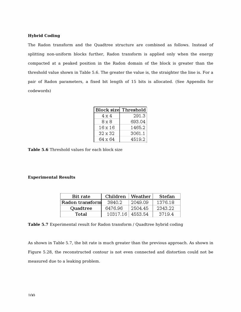
100
Hybrid Coding
The Radon transform and the Quadtree structure are combined as follows. Instead of
splitting non-uniform blocks further, Radon transform is applied only when the energy
compacted at a peaked position in the Radon domain of the block is greater than the
threshold value shown in Table 5.6. The greater the value is, the straighter the line is. For a
pair of Radon parameters, a fixed bit length of 15 bits is allocated. (See Appendix for
codewords)
Table 5.6 Threshold values for each block size
Experimental Results
Table 5.7 Experimental result for Radon transform / Quadtree hybrid coding
As shown in Table 5.7, the bit rate is much greater than the previous approach. As shown in
Figure 5.28, the reconstructed contour is not even connected and distortion could not be
measured due to a leaking problem.

101
Figure 5.28 Radon transform/Quadtree hybrid coding and reconstructed image(right)
Conclusion
The bit rate of the Quadtree structure occupies a large portion of bit rate. The reason is as
follows. The Quadtree does not split blocks in a way that a block has a perfectly straight
line. Hence, most blocks are not qualified to be encoded by Radon transform and rely on the
conventional Quadtree coding. On the other hand, applying Radon transform to a block with
even line-like curve causes disconnected contour.
Secondly, the bit rate of Radon transform is still high. The fixed bit rate allocation for
Radon transform parameter could be quantized depending on block’s size as small block
does not require a fine angle interval. In next section, we attempt to fix such drawbacks.

102
5.3.2 Chain Code / Quadtree Hybrid Coding
As mentioned in the previous section, Radon transform has led to low quality and high bit
rate compression scheme. We propose a conceptual scheme that reduces the Radon
parameters to one as well as facilitates a quantisation of the angle resolution according to
block size.
Instead of Radon transform, chain coding scheme can be substituted. A great
advantage of chain coding is high coding efficiency as each chain code is relatively encoded
to its previous chain code. The Quadtree structure is adopted to control the size of MGCC
cell, as mentioned, MGCC scheme needs variable cell size structure for further
improvement.
Figure 5.29 Various size of MGCC cell
The proposed scheme can be described as follows. The bounding box is partitioned
using the same principle as in the previous approach. Each block is treated as a MGCC cell
and blocks are inter-connected as chain. Various cell sizesare applied to corresponding
block size as shown in Figure 5.29. In this way, by relativity of the chain code, each block
can be encoded by only one parameter representing an angle of the line because line begin
where the line ended in the previous block. Figure 5.30 is an illustration of Chain /
Quadtree hybrid coding scheme.

103
Figure 5.30 Chain code / Quadtree hybrid coding
In theory, it provides better efficiency than the previous method in addition to promising
feature, the block-based compatibility. This is the important issue because the most contour
coding suffers from incompatibility with the conventional block-based motion coding and
texture coding.
Figure 5.31 Prune tree segmentation and Prune-Join tree segmentation
However, still a few of drawbacks found in the previous approach remains. Firstly,
efficient compression of Quadtree structure is required as it occupies a huge portion of the
resulting bit rate. Improvement can be made by joining sub-blocks as shown in Figure 5.31

104
so that each block contains a line from vertex to vertex of polygon. Secondly, reliable rules
to decide whether to split block further or apply chain structure on the block is not defined
in this approach.
5.4 Temporal Prediction
Shape coding techniques presented so far do not take advantage of temporal redundancies
in the scene. In the framework of video sequence coding, it is important to also reduce
temporal redundancy in the bitstream, shapes remaining very similar from frame to frame
as shown in Figure 5.32.
Figure 5.32 Overlapped contour image of 10th and 11th frame of test sequence children

105
5.4.1 Motion Based Prediction Schemes
Shape prediction from frame to frame can be achieved by means of motion estimation and
compensation techniques as described in Section 4.3. A general motion model would handle
shape rotation, scaling and projection. Several shape representation methods invariants to
scaling and rotation have already been investigated [49]. If such a method is applied for
intra-frame shape coding, only motion model parameters need to be transmitted to predict
the shape in the next frame.
In practice however, when shape coding is performed in a complete shape-motion-
texture coder, a scheme consistent with that of texture coding may be used to simplify the
overall algorithm. The main difficulty lies in the dependency between shape, motion and
texture coding. Motion and texture coding are expected to be more efficient when using
shape data. This is the idea behind second generation coding techniques [56]. Temporal
shape coding has been investigated mainly in the framework of region-based coders, where
a spatio-temporal segmentation and tracking algorithm extracts a set of regions coherent
both spatially and temporally [57]. In this case, each region is tracked along the sequence,
and can therefore be temporally predicted from its previous instance. Shape prediction
error results in a set of error regions for which shape or contours can be encoded by one of
several methods, for instance chain codes or skeletons [36].
In block-based coders adapted to perform object scalability, the environment is quite
different. The shape to be coded does not necessarily correspond to a uniform region, but
rather to a preselected object from the scene, possibly including several subregions.
Segmentation is performed semi-automatically based on semantic information (for instance
the number of expected objects), or is available from the image composition stage (blue
screening technique). Motion coding and texture coding remain block-based, but use shape
masking to improve their performance on object boundaries. In this case, when lossy shape

106
coding is performed, the reconstructed shape must be available to perform motion
estimation (only pixels within the shape in the block will be considered). Shape temporal
prediction must then use either former texture-based motion information, or specific motion
vectors that need to be transmitted.
The CAE technique can be straightforwardly extended [27] to the inter mode case to
take advantage of the high correlation between two successive masks. Given a motion
compensated version of the previous mask, a modified template may include pixels from it,
as shown in Section 4.4.Similar steps have been applied to improve the MMR method as
well [30].
Vertex-based methods can be adapted to provide inter-frame coding without too much
effort. In a block-based coder, prediction can be performed from the previous shape, by
exploiting available motion information. This motion can be either specifically computed for
shape information, thus requiring the corresponding parameters to be encoded, or
extrapolated from the texture motion vectors form the previous frame. Each vertex is then
motion compensated and the corresponding error with regard to the contour to
approximate is computed. If the error is lower than the predefined threshold, the vertex is
retained, otherwise it is rejected. The retained vertices constitute a rough polygon to which
the iterative refinement technique presented in Section 5.1.3.2 is applied. The vertex
positions in the old and new lists of vertices are then encoded, for instance by means of a
run-length coding method. Inserted vertices may also be encoded using adaptive arithmetic
coding [53].
Another possibility consists in coding the shape prediction error as a shape image.
However, since the corresponding regions are expected to be small, the corresponding cost
may be higher. Thresholding may be used to eliminate meaningless regions. The tolerance
error should also be adapted to a value different form that used in intra-coding. Similarly to
motion/texture coding schemes, in case no matching is possible, for instance when no
107
motion vector resulting in an acceptable prediction error can be found, the shape is coded
in intra mode.
5.4.2 Entropy Based Prediction Schemes
An alternative temporal prediction technique which does not use any motion information
while it remains lossless may be used at the entropy coding stage. When sophisticated
statistical models are used to code the chain code symbols describing the shape, it is
possible to exploit the experience gained from a previous frame to entropy code the current
frame by maintaining the model from frame to frame, instead of resetting it after each
frame. As an illustration, in the context of chain coding using fixed-order, finite-context
Markov models for arithmetic coding, there exists a simple solution to exploit temporal
redundancies to increase compression ratios. Instead of resetting the probability tables
before each frame, the same tables can be used throughout the sequence. The cost of the
first frame is the same as without exploiting temporal redundancies, but the cost of the
subsequent frames is expected to decreases rapidly.
5.4.3 Chain Based Contour Compensation Scheme
This approach takes advantage of the sequential property of chain code. Once shape
contour is encoded, a certain region of contour may be indexed by order of the
corresponding chain code. For instance, in Figure 5.33 (c), assume A is the kth chain code,
then contour region under chain A can be accessed by referring to A.
The contour motion is usually assumed as translational motion. Using sophisticated

108
contour matching algorithm, choose a best matching contour object in subsequent frame, of
which displacement with the current frame object may be encoded by a global motion
vector. Secondly, the contours are segmented into two regions of matched and mismatched
contour. For mismatched contour, it is needed to decide whether the contour has to be
encoded by new chain codes or split further in order to obtain local motion vectors. In case
that new chain codes are required, chain codes of current object are just removed or new
chain codes are inserted in order to maximizing match using the sequential property
mentioned above. Figure 5.33 is an illustration of such scheme. However, when there is
zooming and/or rotation motion, the translational contour motion may not suit well. In this
case, affine transform may be used [16].
Figure 5.33 Chain -based contour compensation scheme : (a)kth frame (b) k+1th frame (c)
contour overlapped view of the object

109
Chapter 6
Communication Issues
Although the compression efficiency is the most important feature in any compression
scheme, other functionalities and parameters related to reliable network communication,
such as scalability, error resilience, complexity, and delay, to mention a few, should be
taken into account. First, for historical and theoretical reasons, let us look at an abstraction
of the communications problem which leads to the famous separation principle of source
and channel coding [58].
In Shannon’s groundbreaking 1948 paper that laid the foundations of information
theory, he shows that for point-to-point communication over a well-defined channel, a
separate optimisation of source coding and channel coding can lead to a performance
arbitrarily close to the information theoretic bound for the entire system. Therefore,
traditionally, the coding problem has been split into two independent sub-problems, source
compression and channel coding. This has resulted in largely independent research in the
two areas. However, many practical situations do not satisfy the assumption required for
the separation principle to hold. For example, most communication is done with a finite-
delay constraint, which leads to finite block sizes. Under such delay constraints, error
probabilities can be non-negligible, and thus the separation principle has to be revisited.
In such cases, practical schemes using unequal error protection of different parts of
the coded stream are used. For example, in video coding for noisy channels, the motion
vectors are highly protected, since their loss would be catastrophic. Motion residuals,
errors after motion compensation, are much less protected than the motion vectors. In
multiresolution source coders, it is natural to protect more the coarse resolutions, which

110
are absolutely necessary, than the fine details, and this is another instance of unequal error
protection. An interesting application of multiresolution coding is the progressive
transmission of images. Instead of coding at a fixed rate, one has to accommodate diverse
rates, depending on the resolution desired by the particular user accessing the image.
Given a source and a channel, we have to allocate resources to source and channel
coding. The solution turns to be more complicated than expected, and is only partly known
[59]. The question becomes even more intricate when protocol issues are included as in
channels with feedback. However, the protocol issues are out of the scope of this project.
All methods that allow some interaction of the source and the channel coders go under
the name of joint source/channel coding systems. They do not fit the classic separation
principle; rather they solve the practical problem of robust communication when errors do
occur. An instance where the separation principle cannot be used is in the case of multiple
channels, as in broadcast or multicast scenario. Then, users with very different channels
have to be accommodated, which leads to schemes that adapt to the particular channels
they face.
In this section, we propose methods for rate distortion control capability such as
scalable coding and progressive transmission, both based on chain coding, and finally for
bit rate estimation of a given shape object.
6.1 Scalable Coding
As stated above, the rate distortion control is the important feature in visual communication
system. Although chain coding is highly efficient compression, its quality scalability has not
been realized. We propose a conceptual scheme facilitated with rate distortion control
using MGCC.

111
As shown in Figure 6.1, it is possible to use variable sizes of cell depending on condition of
channel. For instance, high speed broadband suits 2x3 or 3x3 cell, hardly producing any
ambiguities in decoding process, hence, resulting the high fidelity of reconstructed contour.
On the other hand, the bigger cells, 4 x 4 cell or larger ones, can be used for low bit rate
connection such as mobile and modem. Furthermore, if one can apply different resolution of
cells to regions according to the human perceptual system effectively without much
overhead bits, then such scheme would be more efficient.
Figure 6.1Scalable coding based on multiple grid chain code
6.2 Progressive Transmission
Secondly, progressive transmission takes advantage of 1/30th of a second to improve
quality of reconstruction, in case of 30 frames per second, before the next frame arrives for
processing. With a few bits transmitted, decoder should be able to reconstruct a coarse
quality contour shape by the scalability (Section 6.1) and as more bits are received the
reconstruction quality becomes better. As an extension to the scheme above, when coarse
shape is reconstructed by large cells, shape quality can be improved. During encoding, for
each cell we can determine whether the reconstructed contour will be different from the
original contour (see Section 5.2.1). Firstly, choose a cell that is already transmitted and

112
represents different contour from the source, and then encode further using smaller cells. If
a relatively small cell such as 3x4 cell is used, a few flag indicating which path the actual
contour take can be transmitted. Figure 6.2 is an illustration of such scheme.
Figure 6.2 Progressive transmission based on chain code
6.3 Bit-Rate Estimation
Thirdly, estimating bit rate of a shape given the limited bandwidth is essential in order to
determine adequate cell size. We introduce Eccentricity as shape bit rate estimation.
Eccentricity is calculated using equations below[60].
(6.1)
where , ,
is the centre of mass.

113
Eccentricity reveals that roughness of contour of shape, closely related to bit rate as
described Section 5.2.3. Figure 6.3 shows correlation of actual bit rate and Eccentricity.
Figure 6.3 Correlation between Eccentricity and Bit rate : (top)Eccentricity and (bottom)
Bit rate of test sequence Children

114
Chapter 7
Conclusion
Object-based representation has been an important paradigm in still as well as moving
images due to its capability to mimic human perceptual system. Shape coding enables
object-based interactivity. Efficiency of shape information compression is of prime
importance. Even interactivity is a demanded feature in various parts of modern
communication, incorporating such functionality could affect overall efficiency of
compression system built upby sophisticated motion and texture algorithms. This project
investigated into shape coding techniques, possible improvement of the MGCC, hybrid
coding and communication related issues.
First of all, various shape coding methods are summarised. Contribution of this project
is described with possible direction of future research. Finally, author’s assessment is
included.
7.1 Summary of Shape Coding Methods and Discussion
In this report, compression of visual data is overviewed beginning with Shannon’s source
coding theorem and simple entropy coding technique. Four classes of major video coding
are reviewed in light of the object-based coding scheme and related video coding standards
such as MPEG and H.264 and the recent trend is addressed. The object-based
representation is addressed in details in terms of inter-operability and problems of shape
coding are discussed. After that, various shape coding approaches are covered. They can be
summarised as follows.

115
Bitmap-Based Coding
In the framework of MPEG-4, the bitmap-based method turns out to be the most efficient in
terms of compression. This superiority is mainly due to the predictive coding, which takes
advantage of the temporal redundancy. These methods are generally quite versatile and can
be adapted to either frame-based or block-based coding environments. (See Section 4.4 and
5.1.1)
Skeleton Decomposition
Skeleton decomposition is a well-known way to intrinsically represent shapes, and has
recently been applied to lossless shape coding. However, the corresponding performance
remains lower than that of chain code-based methods as shown in [36], especially when the
shape can be described by a few long contours. On the other hand, the skeleton
decomposition allows scalable transmission and can offer a graceful degradation when
transmission errors occur by allowing at least a partial reconstruction of the shape. (See
Section 5.1.2.1)
Macro / Quadtree Hybrid Coding
A hybrid Macro/Quadtree representation is well suited for low-delay applications since each
macroblock is coded independently. This also facilitates error resilience. Progressive
transmission can be obtained by exploiting the Quadtree hierarchical representation.
However, the corresponding compression performance remains poor. A simple rate-
distortion control based on a specific pre-processing step can be used, but the resulting
image degradation is not graceful. (See Section 5.1.2.2)

116
General Contour Based Coding
Contour oriented coding schemes provide a semantic representation suitable for some
applications such as indexing and retrieval. However, their efficiency decreases when the
shape is a collection of small disjoint regions, and their integration in a block -based coder
is not straightforward. (See Section 5.1.3)
Chain Coding
The chain coding method provides the most efficient contour-based lossless compression
scheme. Current schemes have poor rate distortion control, poor scalability, and poor error
robustness. Further research is needed in order to make the chain coding method more
versatile, possibly by combining it with geometrical contour approximation. (See Section
5.1.3.1 and Section 5.2.2)
Among the highly efficient chain codes, the MGCC shows great potentials in intra-,
inter- frame coding as well as scalable coding. For intra-coding, its efficiency is improved by
the proposed scheme and further improvement is also possible. For inter-coding, using
entropy coding model, or chain based contour compensation is expected to perform well.
Based on contour simplification mechanism of the scheme, rate-distortion control is also
feasible. These topics are summarised in Section 7.2
Geometrical Representation
The main strength of geometrical approximation methods lies in their capability to
gracefully degrade the shape quality as the maximum allowable error constraint is relaxed,
thus easily providing a rate-distortion control. Lossless coding may be achieved by setting
this error to zero, however, most shapes are not simple enough for this technique to
outperform the chain coding methods in that case. On the other hand, such methods may be
very useful for representing noisy masks, since they naturally filter the shape. Progressive

117
transmission can also be achieved by transmitting vertices in a specific order allowing
shape reconstruction from the coarsest to the finest description. The error resilience is
slightly better than for chain coding, depending on whether absolute or differential coding
of the vertices is performed. (See Section 5.1.3.2)
7.2 Topics for Future Research
In this section, we suggests interesting topics, extended parts of the project, to pursue
which could not be completed due to insufficient time. The detailed description of
conceptual design of each topic is described in main text and we here review such topics
briefly.
Interaction with Block-Based Coding
As mentioned previously, compatibility with texture and motion coding is important. Since
shape information narrows down a range of pixels that texture and motion coding algorithm
need to consider, it enhances efficiency. For that reason, it is more efficient to inter-
perform those coding algorithms for a pixel or a group of pixels. As shown in Section 5.3.2,
theoretically chain / Quadtree hybrid coding provides interesting features. Since it take
advantage of Quadtree structure to vary cell dimension at the expense of additional bit rate.
The scheme is indeed block-based with respect to the Quadtree, contrarily, is contour-
based scheme with respect to use of chain code. It may not outperform pure contour-based
methods, instead, does provide compatibility with block -based scheme.(See Section 5.3.2)

118
Entropy Based Prediction / Contour Compensation
In the framework of video communication, the performance of shape coding schemes can
be improved by taking temporal redundancies into account as well. One approach,
specifically suitable for lossless chain code methods, consists in exploiting temporal
redundancy at the entropy coding level. Another approach, expected to be more efficient
uses motion estimation and compensation to predict shape changes from frame to frame.
Lastly, contour compensation takes advantage of sequential property of chain code. Rather
than partitioning VOP into sub blocks and encoding by motion vector, a specific region of
contour is accessible by the order of the corresponding chain code. This also preserves
contour-based structure. (See Section 5.4.2 and Section 5.4.3)
Scalability /Progressive Transmission
For most applications, high compression rates are desirable, since storage space and
bandwidth are often at a premium. For low bandwidth applications, such as video
telephony, the goal is to utilise as much as possible of the available bandwidth. Rate-
distortion control schemes are thus needed to get the lowest distortion for a given rate. For
multimedia client-server applications, scalability is desirable. After a few bits have been
transmitted, the receiver should be able to render a coarse approximation of the shape,
which is then refined as more bits are received. For networking applications, error
resilience is desirable. The loss or damaging of a packet should not completely ruin the
reconstruction of the shape.
The chain coding is lossless compression method with poor rate-distortion control, etc.
as described in Section 7.1. Scalable coding based on the MGCC has not been realised in
any literature. However, the scalability can be achieved by relaxing a fixed cell dimension
constraint. (See Chapter 6)

119
Conclusion
In conclusion, a lot of research still needs to be done in the field of coding the shape of
video objects. Future possible solutions may lie in hybrid coding schemes mixing different
shape representation methods, such as a scalable chain coding method as extension of
polygonal approximation (based on flexible directionality and anisotropy), or the use of a
semantic shape representation in intra-frames for high-level random access combined with
an efficient block-based temporal coding method. Moreover, when designing any shape
coding algorithm, attention should be paid not only to compression efficiency, but also to
interaction with texture coding, to rate-distortion control capability and additional
functionalities such as error robustness and scalability. Error resilience for chain coding
still remains to solved.
7.3 Contributions and Author’s Assessment
At the beginning, the goal of this project was developing an efficient shape coding
algorithm named Multiple Grid Chain Codes (MGCC). The MGCC, which evolved from the
differential chain code by exploiting psychovisual redundancy, has been investigated in
details and improvement over the scheme has been attempted at various angles.
Based upon the directionality and the anisotropy exploiting contour coherence, the
efficiency of the MGCC has been greatly improved at most 20% gain while the resulted
distortion is even lower besides its low computational complexity remains same. This
improvement equals more than 50% gain over the original Freeman code. This has led to a
publication titled as “Lossless shape representation using Multiple Grid Chain Code”.

120
Then a goal of the project was extended to investigate various aspects of shape coding
related to communication such as scalable coding, progressive transmission, rate-distortion
capability as well as further possible improvement using hybrid coding. Particularly, the
proposed Chain / Quadtree hybrid scheme has shown theoretic interests. Namely high
intra-frame coding efficiency based on integration of the contour based structure of the
MGCC with block-based scheme that may offer great advantage of compatibility with
other block-based scheme such as block-based motion and texture coding. Also, the
proposed chain based contour compensation, which exploits inter-frame redundancy while
preserving chain code structure as most contour-based approach suffers from sub-
optimal inter-frame coding efficiency.
Other valuable findings are as follows. A ways to facilitate scalability to chain code
structure which enables chain codes to control shape bit rates, which is essential in
communication system and a method to estimate bit rate of object using eccentricity. The
result of those schemes is likely to be used to produce two more potential publications.
Finally, based on such findings above I would describe the project as a success.

121
122
Appendix
A. Software Documentation
A.1 Coder Implementation
The coder is implemented using Java 1.4.2 and its static model is illustrated in Figure A.1.
The implementation works as follows. First of all, FileLoader class extracts bitstream for a
designated frame. The extracted bitstream is passed to Encoder. Secondly, a BinaryImage
is created by parsing the bitstream. The hexagonal grid is super-imposed on the image by
spacing one pixel between every two adjacent pixels vertically and horizontally. Then, an
active edge, an edge between black and white pixels, are searched from left to right and
from top to bottom order. Once an active edge is met during the raster scan, an instance of
ShapeObject class is created and the coordinates of the edge are recorded in that object as
the starting point and contour encoding process begins using Cell. During encoding, the
boundary information is also stored in that object by which we can distinguish objects. The
encoded contour information, namely exits of each cell, is stored in java.util.Vector object
and Huffman coded. Then scan continues up to the final pixel. The decoding process is
exactly the reversed process. Note that it is not guaranteed that the last active edge in a
contour coincides with the initial active edge. This might produce unnaturally reconstructed
contour as shown in FigureA.2 and also cause problems when reconstructed contour is
filled. Hence, a adequate post-processing is required. The boundary information is also
stored when objects are reconstructed and is used when filling the reconstructed object.
For hybrid coding scheme are designed similarly, but quadtree is used instead of cell.
Substituting the Quadtree class for the Cell class in Figure A.1 shows its static model.

123
Figure A.1 Static modelling of MGCC coder (NewCell : provision for improved MGCC cell)
Figure A.2 Unnaturally reconstructed contour (light shaded pixel: outside the object, dark
shaded pixel: inside the object, shaded edge: starting edge)

124
A.2 Organisation and Compilation
Source contents distributed with this report is organised by six directories. Each directory
contains coders which are based on approaches mentioned in Section 5.2.2. Each coder can
be compiled independently, executed by java Encoder, and ported to any platform as it is
written in Java.
/source includes test sequence used in this project; children, weather and stefan
/mgcc contains MGCC coder (See Section 5.2.1)
/new contains a coder based on the proposed scheme using directionality and
anisotropy (See Section 5.2.2.5 (i))
/new2 contains a coder based on the same scheme but producing less distortion.
(See Section 5.2.2.5 (ii))
/new2x3 contains a coder based on the same scheme but using 2x3 cell
(See Section 5.2.2.5 (iii)
/new3 contains a coder based on another proposed scheme using a template.
(See Section 5.2.2.5 (iv))
/block contains a block-based coder using Radon transform and Quadtree
(See Section 5.3.1)
However, the coder under block directory requires Matlab and a toolkit, JMatLink, whick
allows interaction between Matlab and Java, is available only on Windows platform.
JMatLInk is available at ‘http://www.held-mueller.de/JMatLink/’

125

126
B. Graphical Experimental Result
<Bit Rate of children>
<Distortion Rate of children>

127
<Bit Rate of Weather>
<Distortion Rate of Weather>
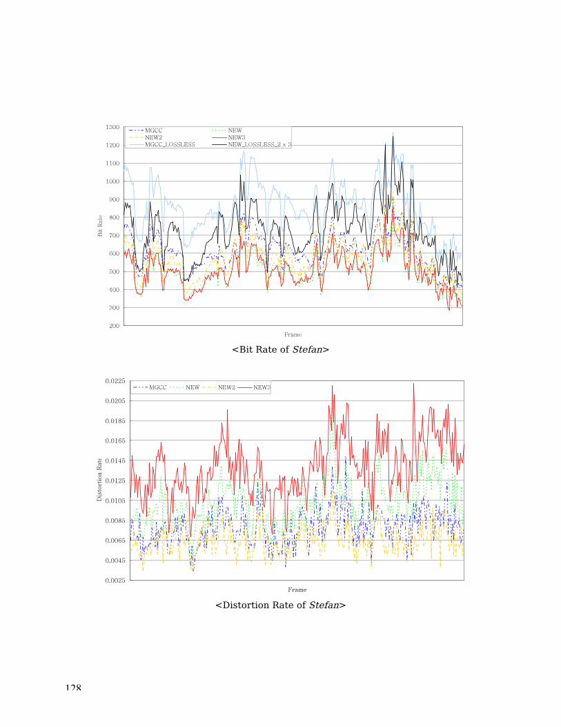
128
<Bit Rate of Stefan>
<Distortion Rate of Stefan>

129

130
C. Probability of Symbols and Corresponding Codewords
<MGCC>
<NEW1Approach>
0 5
10 15 20 25 30 35
1 2 3 4 5 6 7 Exit
%
0
5
10
15
20
25
1 2 3 4 5 6 7 8 9 Exit
%

131
<NEW2 Approach, more codewords are defined for specific path>
< NEW 1 APPROACH, 2 x 3 Cell for Lossless compression>
0
5
10
15
20
25
1. 2. 3. 3A. 3B. 4. 4A. 5. 6. 7. 8. 9. Exit
%
0
5
10
15
20
25
30
1 2 3 4 5 Exit
%

132
<NEW 3 Approach>
<NEW 4 Approach>
Black, White, Split, and Radon represent uniformly black block, uniformly white block,
indication for splitting block and indication for Radon parameters respectively
0 5
10 15 20 25 30 35
1 2 3 4 5 6 7 8 9 10 11 12 Cell
%
0
10
20
30
40
50
60
Black White Split 2x2L 2x2R Radon
%

133

134
D. Bibliography
[1] H. Musmann, M. Hötter, and J. Ostermann, “Object-oriented analysis-synthesis
coding of moving images”, Signal Process., Vol. 1, pp. 117-138, Oct 1989
[2] M. Kunt, “Second-generation image coding techniques”, Proc. IEEE, Vol. 73, pp.
549-574, Apr. 1985
[3] N. Brady, “MPEG-4 Standardized Methods for the Compression of Arbitrarily Shaped
Video Objects”, IEEE Trans. CSVT., Vol. 9, pp. 1170-1189, Dec. 1999
[4] C. E. Shannon, “A mathematical theory of communication”, Bell Systems Technical
Jounal, Vol. 27, pp. 379-423, 623-656, 1948
[5] Jacob Ziv and Abraham Lempel, “A universal algorithm for sequential data
compression”, IEEE Trans. IT., Vol.23, pp.337-343, May 1977
[6] Jacob Ziv and Abraham Lempel, “Compression of individual sequences via variable-
rate coding”, IEEE Trans. IT., Vol. 24, pp. 530-536, Sep 1978
[7] G. Karlsson and M. Vetterli, “Three dimensional subband coding of video”, Proc.
IEEE ICASSP, Vol. 2, pp. 1100-1103, Apr 1988
[8] J. R. Ohm, “Temporal domain subband video coding with motion compensation”,
Proc. IEEE ICASSP, Vol. 3, pp. 229-232, Mar 1992
[9] M. Gilge, “A high quality videophone coder using hierarchical motion estimation and
structure coding of the prediction error”, Proc. SPIE Conf. VCIP, Vol. 1001, pp. 864-
874, Nov 1988
[10] Y. –Q. Zhang and S. Zafar, “Motion-compensated wavelet transform coding for color
video compression”, Proc. SPIE Conf. VCIP, Vol. 1605, pp. 301-316, Nov 1991
[11] M. Kunt, A. Ikonomopoulos, and M.Kocher, “Second-generation image coding
techniques”, Proc. IEEE, Vol. 73, pp. 549-574, Apr 1985

135
[12] M. Kocher and M. Kunt, “Image data compression by contour texture modeling”,
Proc. SPIE Int. Conf. Application of Digital Image Processing, Geneva, Switzerland,
pp.131-139, Apr 1983
[13] S. Carlsson, “Sketch-based coding of grey level images”, Signal Proc., Vol. 15, No. 1,
pp. 57-83, Jul 1988
[14] M. Kunt, M. Benard, and R. Leonardi, “Recent results in high compression image
coding”, IEEE Trans. Circuits Syst., Vol CAS-34, pp. 1306-1336, Nov 1987
[15] P. Salembier, L. Torres, F. Meyer, and C. Gu, “Region-based coding using
mathematical morphology”, Proc. IEEE, Vol. 83, pp. 843-857, Jun 1995
[16] H. Jozawa and H. Watanabe, “Video coding using segment based affine motion
comprensation” Proc. Picture Coding Symposium, Sacramento, CA, pp. 238-241 Sep
1994
[17] H. H. Chen, M. R. Civanlar, and B. G. Haskell, “ A block transform coder for
arbitrarily shaped image segments”, Proc. IEEE ICIP, Vol. 1, pp. 85-89, Nov 1994
[18] Y.Yokohama, Y. Miyamoto, and M. Ohta, “very low bit-rate video coding with object-
based motion compensation and orthogonal transform,” in Proc.SPIE Conf. VCIP,
Nov.1993, vol. 2049, pp. 12-23.
[19] M. F. Barnsley, “Fractals Everywhere”, San Diego, CA: Academic, 1988
[20] A. E. Jacquin, “Image coding based on a fractal theory of iterated contractive image
transformation,” IEEE Trans. Image Processing, vol. 1, pp. 18-30, Jan. 1992.
[21] K. Barthel, T. Voy’e, and P. Noll, “Improved fractal image coding,” Proc. Picture
Coding Symp. (PCS), Lausanne, Switzerland, Mar. 1993, no. 1.5.
[22] J. M. Beaumont, “Image data compression using fractal techniques,” Br.
Telecommun. Technol. J., Vol. 9, no. 4, pp. 93-109, Oct. 1991
[23] H. Li, M. Novak, and R. Forchheimer, “fractal-based image sequence compression
scheme,” Opt. Eng., vol. 32, no. 7, pp. 1588-1595, July 1993

136
[24] Zhen Yao, “Fractal Coding and Its Applications” BSc Thesis, Dept. of Computer
Science, Univ. of Warwick, Sep 2003
[25] E. Reusens, “Sequence coding based on the fractal theory of iterated transformation
systems,” Proc. SPIE Conf. VCIP., Nov. 1993, vol. 1, pp. 132-140
[26] K. Aizawa, H. Harashima, and T. Saito, “model-based analysis synthesis image
coding (MBASIC) system for a person’s face,” Signal Process., Vol. 1, no. 2, pp. 139-
152, Oct. 1989
[27] Noel Brady and Frank Bossen, “Shape compression of moving objects using context-
based arithmetic encoding”, Signal Proc. Image Comm. Vol. 15, pp. 601-617, 2000
[28] D. Ballard and C. Brown, “Computer Vision”, Prentice Hall, 1982
[29] R. Mehrotra and J.E. Gary. “Similar shape retrieval in shape data management”,
Computer, Vol. 28, pp. 57. 57-62
[30] N. Yamaguchi, T. Ida, and T. Watanabe, “A binary shape coding method using
modified MMR”, ICIP, Oct 1997
[31] I. Witten, R. Neal, and J. Cleary, “Arithmetic coding for data compression”, Commun.
ACM, Vol. 30, pp. 520-540, Jun 1987
[32] F. Bosson and T. Ebrahimi, “A simple and efficient binary shape coding technique
based on bitmap representation”, ICASSP, 1997
[33] C. R. Dyer, A. Rosonfeld, and H. Samet, “Region representation: boundary codes
from quadtree”, Commun. ACM, Vol. 23, No. 3, pp. 171-179, Mar 1980
[34] M. Etoh, C.S. Boon, and S. Kadono, “Template-based video coding with Opacity
representation”, IEEE, Trans. on Circuits, Systems and Video Tech., Vol. 7, pp. 172-
180, Feb 1997
[35] L. Shapiro, R. MacDonald, and S. Sternberg, “Ordered structural shape matching
with primitive extraction by mathematical morphology”, Pattern Recognition, Vol.
20, pp. 75-90, 1987

137
[36] P. Brigger, “Morphological shape representation using the skeleton decomposition:
application to image coding”, PhD thesis, EPFL, Lausanne, Switzerland, 1995
[37] P. A. Margos and R. W. Schafer, “Morphological skeleton representation and coding
of binary images”, IEEE Trans. on Acoustics, Speech and Signal Proc., Vol. 34, pp.
1228-1244, Oct 1986
[38] H. Freeman, “On the encoding of arbitrary geometric configurations”, IRE Trans.
Electronics Computers, EC-10, pp. 260-268, Jun 1961
[39] A. Rosenfeld and A. C. Kak, “Digital Picture Processing”, Vol. 2, Academic Press,
New York, USA, 2nd edition, 1982
[40] H. Freeman, “Computer Processing of Line Drawing Images”, Computing Surveys,
Vol. 6, pp. 57-97, Mar 1974
[41] Ad hoc group on Shape Coding, Description of core experiments on shape coding.
Technical Report JTC1/SC29/WG11/M0889, ISO/IEC, May 1996
[42] T. Kaneko and M. Okudaira, “Encoding of arbitrary curves based on chain code
representation”, IEEE Trans. Commun., Vol. 33, pp. 697-707, Jul 1985
[43] M. Eden and M. Kocher, “On the performance of a contour coding algorithm in the
context of image coding Part 1: Contour Segment Coding”, Signal Proc., Vol. 8, pp.
381-386, 1985
[44] C. Lu and J. Dunham, “Highly efficient coding schemes for contour line based on
chain code representations”, IEEE Trans. Commun., Vol. 39, pp. 1511-1514, Oct
1991
[45] P. Nunes, F. Marques, “A contour based approach to binary shape coding using a
multiple grid chain code”, Signal Processing : Image Commun. Vol. 15, pp. 585-599
[46] J.D. Foley, A. van Dam, .K. Feiner, and J.F. Hughes, “Computer graphics: principles
and practice”, Addison-Wesley, 2nd edition, 1990
[47] B. Ray and K. Ray, “An optimal algorithm for polygonal approximation of digitized
curves using l1 norm”, Pattern Recognition, Vol. 26, pp .505-509

138
[48] U. Ramer, “An iterative procedure for polygonal approximation of plane curves”,
Computer Graphics and Image Processing, Vol. 1, pp. 244-256, 1972
[49] B. Ray and K. Ray. “A new split-and-merge technique for polygonal approximation of
chain coded curves”, Pattern Recognition Letter, Vol.16, pp. 161-169, Feb 1995
[50] J. Dunham, “Optimum uniform piecewise linear approximation of planar curves”,
IEEE Trans., PAMI., Vol. 8, pp. 57-75, Jan 1986
[51] K.W. Stuhlmuller, A. Salai, and B. Girod, “Rate-constrained contour representation
for region-based motion compensation” Proc. Symp. on Visual Commun. and Image
Process., SPIE, Vol. 2727, Mar 1996
[52] C. Gu, “Multivalued morphology and segmenteation-based coding”, PhD thesis,
EPFL, Lausanne, Switzerland
[53] P. Gerken, “Object-based analysis-synthesis coding of image sequences at very low
bit rates”, IEEE Trans. on Circuits, Systems and Video Tech., Vol. 4, pp. 228-235,
1994
[54] C. Gu and M. Kunt, “Contour Simplification by a New Nonlinear Filter for Region-
based Coding”, IEEE ICIP., Vol. 3, pp. 751-755, 1994
[55] Ning Chen, “Shape Coding For Arbitrarily Shaped Object”, MSc Thesis, Dept. of
Computer Science, Univ. of Warwick, Sep 2002
[56] M. Kunt, A. Ikonomopoulos, and M. Kocher, “Second generation image coding
techniques”, Proc. IEEE, Vol. 73, pp. 549-575, 1985
[57] S. Ayer, “Sequential and Competitive Methods for Estimation of Multiple Motions”,
PhD thesis, EPFL, Lausanne, Switzerland, 1995
[58] T. M. Cover and J. A. Thomas, “Elements of Information Theory”, Wiley Interscience,
New York, NY, 1991
[59] B. Hochwowald and K. Zeger, “ Trade-odd between source and channel coding,”
IEEE Trans. On Inform. Th., Vol. 43, No. 5, pp. 1412-1424, Sep 1997

139
[60] ISO/IEC JTC 1/SC 29 M4242, Text of 15938-5 FDIS Information Technology --
Multimedia Content Description Interface -- Part 5 Multimedia Description Schemes,
pp. 70-71, Oct 2001