Shape-from-Polarimetry:A New Tool for Studying the Air-Sea Interface

Shape-from-Polarimetry:A New Tool for Studying the Air-Sea Interface

Howard Schultz, UMass Amherst, Dept of Computer ScienceChris J. Zappa, Michael L. Banner, Russel Morison, Larry Pezzaniti

Howard Schultz, UMass Amherst, Dept of Computer ScienceChris J. Zappa, Michael L. Banner, Russel Morison, Larry Pezzaniti

Introduction

• What is Polarimetry– Light has 3 basic qualities– Color, intensity and polarization– Humans do not see polarization

Introduction

Linear Polarization

http://www.enzim.hu/~szia/cddemo/edemo0.htm

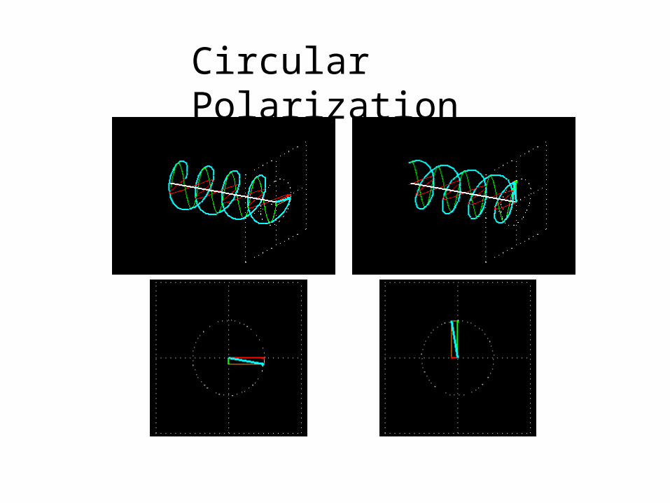
Circular Polarization

• A bundle of light rays is characterized by intensity, a frequency distribution (color), and a polarization distribution

• Polarization distribution is characterized by Stokes parametersS = (S0, S1, S2, S3)

• The change in polarization on scattering is described by Muller Calculus SOUT = M SIN

• Where M contains information about the shape and material properties of the scattering media

• The goal: Measure SOUT and SIN and infer the parameters of M

Muller Calculus

Amount of circular polarizationOrientation and degree of linear polarizationIntensity

Incident LightMuller MatrixScattered Light

Shape-from-Polarimetry (SFP)

• Use the change in polarization of reflected or refracted skylight to infer the 2D surface slope, , for every pixel in the imaging polarimeter’s field-of-view

€

∂z /∂x and ∂z /∂y

Shape-from-Polarimetry

€

RAW =

α +η α −η 0 0

α −η α +η 0 0

0 0 γ Re 0

0 0 0 γ Re

⎡

⎣

⎢ ⎢ ⎢ ⎢

⎤

⎦

⎥ ⎥ ⎥ ⎥

and TWA =

′ α + ′ η ′ α − ′ η 0 0

′ α − ′ η ′ α + ′ η 0 0

0 0 ′ γ Re 0

0 0 0 ′ γ Re

⎡

⎣

⎢ ⎢ ⎢ ⎢

⎤

⎦

⎥ ⎥ ⎥ ⎥

€

α =1

2

tan θ i −θ t( )

tan θ i +θ t( )

⎡

⎣ ⎢

⎤

⎦ ⎥

2

η =1

2

sin θ i −θ t( )

sin θ i +θ t( )

⎡

⎣ ⎢

⎤

⎦ ⎥

2

γRe =tan θ i −θ t( ) sin θ i −θ t( )

tan θ i +θ t( ) sin θ i +θ t( )

€

′ α =1

2

2sin ′ θ i( ) sin ′ θ t( )

sin ′ θ i + ′ θ t( ) cos ′ θ i + ′ θ t( )

⎡

⎣ ⎢

⎤

⎦ ⎥

2

′ η =1

2

2sin ′ θ i( ) sin ′ θ t( )

sin ′ θ i + ′ θ t( )

⎡

⎣ ⎢

⎤

⎦ ⎥

2

′ γ Re =4 sin2 ′ θ i( ) sin2 ′ θ t( )

sin2 ′ θ i + ′ θ t( ) cos2 ′ θ i + ′ θ t( )

S = SAW + SWA

SAW = RAWSSKY and SWA = TAWSUP

€

sin θ i( ) = n sin θ t( ) and sin ′ θ i( ) =1

nsin ′ θ t( )

Kattawar, G. W., and C. N. Adams (1989), “Stokes vector calculations of the submarine light-field in an atmosphere-ocean with scattering according to a Rayleigh phase matrix - Effect of interface refractive-index on radiance and polarization,” Limnol. Oceanogr., 34(8),1453-1472.

Shape-from-Polarimetry

• For simplicity we incorporated 3 simplifying assumptions– Skylight is unpolarized SSKY = SSKY(1,0,0,0)

good for overcast days– In deep, clear water upwelling light can be neglected SWA =

(0,0,0,0). – The surface is smooth within the pixel field-of-view

€

DOLP θ( ) =S1

2 + S22

S02 and φ =

1

2tan−1 S2

S1

⎛

⎝ ⎜

⎞

⎠ ⎟+ 90°

Shape-from-Polarimetry

Sensitivity = (DOLP) / θ

Experiments

• Conduct a feasibility study– Rented a linear imaging polarimeter– Laboratory experiment

• setup a small 1m x 1m wavetank• Used unpolarized light• Used wire gauge to simultaneously measure wave profile

– Field experiment• Collected data from a boat dock• Overcast sky (unpolarized)• Used a laser slope gauge

Looking at 90 to the wavesLooking at 45 to the wavesLooking at 0 to the waves

Slope in Degrees

X-Component

Y-Component

X-Component Y-Component

Slope in Degrees

Build an Imaging Polarimeter for Oceanographic Applications – Polaris Sensor Technologies

– Funded by an ONR DURIP– Frame rate 60 Hz– Shutter speed as short as 10 μsec–Measure all Stokes parameters–Rugged and light weight–Deploy in the Radiance in a Dynamic Ocean

(RaDyO) research initiativehttp://www.opl.ucsb.edu/radyo/

Motorized Stage12mm travel5mm/sec max speed

ObjectiveAssembly

Polarizing beamsplitterassembly

Camera 1(fixed)

Camera 2

Camera 3Camera 4

Air-Sea Flux Package

Imaging Polarimeter

Scanning Altimeters and Visible Camera

~36°

Deployed during the ONR experimentRadiance in a Dynamic Ocean (RaDyO)

Analysis & Conclusion

• A sample dataset from the Santa Barbara Channel experiment was analyzed

• Video 1 shows the x- and y-slope arrays for 1100 frames• Video 2 shows the recovered surface (made by integrating the

slopes) for the first 500 frames

Time series comparison

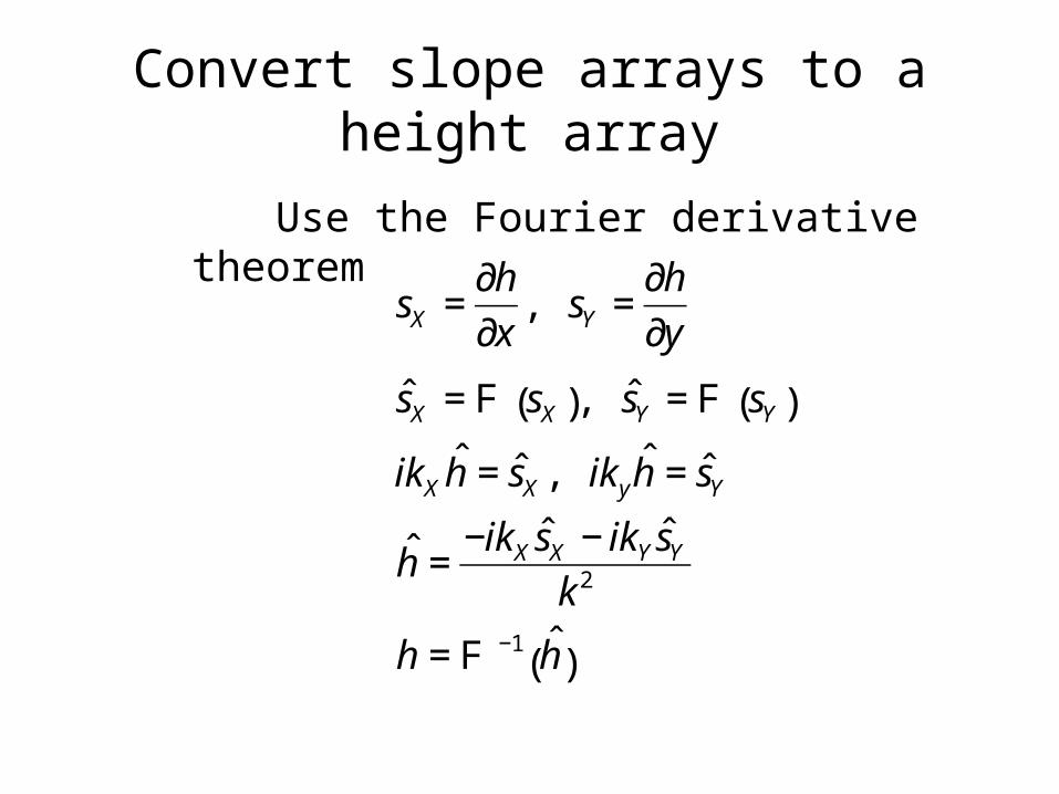
Convert slope arrays to a height array

Convert slope arrays to a height array (Integration)

Convert slope arrays to a height array

Use the Fourier derivative theorem

€

sX =∂h

∂x, sY =

∂h

∂y

ˆ s X = F sX( ), ˆ s Y = F sY( )

ikXˆ h = ˆ s X , iky

ˆ h = ˆ s Y

ˆ h =−ikX

ˆ s X − ikYˆ s Y

k 2

h = F −1 ˆ h ( )

Reconstructed Surface Video

Analysis & Conclusion

• The shape-from-polarimetry method works well for small waves in the 1mm to 10cm range.

• Need to improve the theory by removing the three simplifying assumptions– Skylight is unpolarized SSKY = SSKY(1,0,0,0)

– Upwelling light can be neglected SWA = (0,0,0,0). – The surface is smooth within the pixel field-of-view

• Needs to have an independent estimate of lower frequency waves.

Seeing Through Waves

• Sub-surface to surface imaging• Surface to sub-surface imaging

Optical Flattening

Optical Flattening

• Remove the optic distortion caused by surface waves to make it appear as if the ocean surface was flat– Use the 2D surface slope field to find the refracted

direction for each image pixel– Refraction provides sufficient information to

compensate for surface wave distortion– Real-time processing

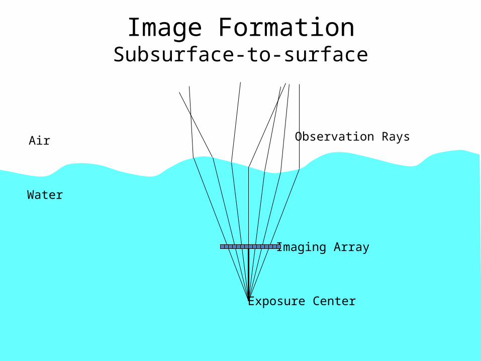
Image FormationSubsurface-to-surface

Imaging Array

Exposure Center

Observation RaysAir

Water

Image Formationsurface-to-subsurface

Imaging Array

Exposure Center

Air

Water

Imaging Array

Exposure Center

Seeing Through Waves

0 20 40 60 80 0 10 20 30 40

Seeing Through Waves

Optical Flattening

• Remove the optic distortion caused by surface waves to make it appear as if the ocean surface was flat– Use the 2D surface slope field to find the refracted

direction for each image pixel– Refraction provides sufficient information to

compensate for surface wave distortion– Real-time processing

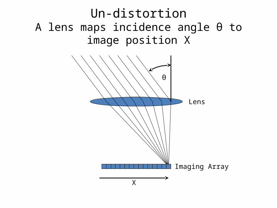
Un-distortionA lens maps incidence angle θ to image position X

Lens

Imaging Array

X

θ

X

θ

Lens

Imaging Array

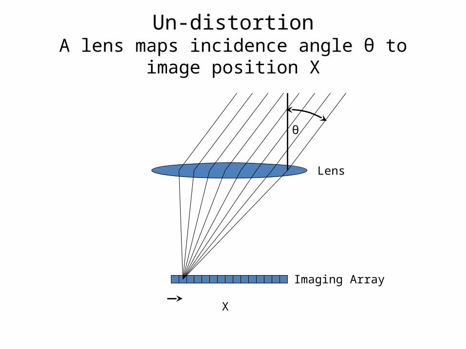
Un-distortionA lens maps incidence angle θ to image position X

X

Lens

Imaging Array

Un-distortionA lens maps incidence angle θ to image position X

X

θ

Lens

Imaging Array

Un-distortionA lens maps incidence angle θ to image position X

X

θ

Lens

Imaging Array

Un-distortionA lens maps incidence angle θ to image position X

Distorted Image Point

Image array

Un-distortionUse the refraction angle to “straighten out” light rays

Air

Water

Un-distorted Image Point

Image array

Un-distortionUse the refraction angle to “straighten out” light rays

Air

Water

Real-time Un-Distortion

• The following steps are taken Real-time Capable– Collect Polarimetric Images ✔– Convert to Stokes Parameters ✔– Compute Slopes (Muller Calculus) ✔– Refract Rays (Lookup Table) ✔– Remap Rays to Correct Pixel ✔

Image Formationsurface-to-subsurface

Imaging Array

Exposure Center

Air

Water

Imaging Array

Exposure Center

Detecting Submerged Objects“Lucky Imaging”

• Use refraction information to keep track of where each pixel (in each video frame) was looking in the water column

• Build up a unified view of the underwater environment over several video frames

• Save rays that refract toward the target area• Reject rays that refract away from the target area

For more information contactHoward SchultzUniversity of MassachusettsDepartment of Computer Science140 Governors DriveAmherst, MA 01003Phone: 413-545-3482Email: hschultz@cs.umass.edu