sharif university of technologyce.sharif.edu/courses/91-92/1/ce717-2/resources/root/lectures... ·...

Gradient Descent CE-717: Machine Learning Sharif University of Technology

M. Soleymani

Fall 2012

Some slides have been adapted from: Prof. Ng (Machine Learning, Online Course, Stanford)

Iterative optimization

2

Cost function: 𝐽(𝒘)

Optimization problem: 𝒘 = argm𝑖𝑛𝒘

𝐽(𝒘)

Steps:

Start from 𝒘0

Repeat

Update 𝒘𝑡 to 𝒘𝑡+1 in order to reduce 𝐽

𝑡 ← 𝑡 + 1

until we hopefully end up at a minimum

Gradient descent

3

Minimize 𝐽(𝒘)

𝒘𝑡+1 = 𝒘𝑡 − 𝜂𝛻𝒘𝐽(𝒘

𝑡)

𝛻𝒘𝐽 𝒘 = [𝜕𝐽 𝒘

𝜕𝑤1,𝜕𝐽 𝒘

𝜕𝑤2, … ,

𝜕𝐽 𝒘

𝜕𝑤𝑑]

Learning rate

parameter

Gradient descent

Cost function: Sum of squares error

4

Minimize 𝐽(𝒘)

𝒘𝑡+1 = 𝒘𝑡 − 𝜂𝛻𝒘𝐽(𝒘

𝑡)

𝐽(𝒘): Sum of squares error

𝐽 𝒘 = 𝑦 𝑖 − 𝑓 𝒙 𝑖 ; 𝒘2𝑛

𝑖=1

Gradient descent:

Cost function: Sum of squares error

5

Weight update rule: linear assumption 𝑓 𝒙;𝒘 = 𝒘𝑇𝒙

𝒘𝑡+1 = 𝒘𝑡 + 𝜂 𝑦 𝑖 −𝒘𝑇𝒙 𝑖 𝒙(𝑖)𝑛

𝑖=1

𝜂: too small → gradient descent can be slow.

𝜂 : too large → gradient descent can overshoot the

minimum. It may fail to converge, or even diverge.

Batch mode: each step

considering all training data

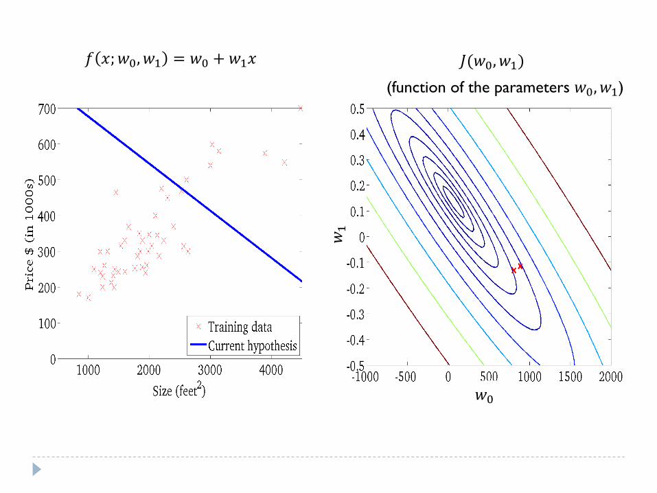
(function of the parameters 𝑤0, 𝑤1)

𝑓 𝑥;𝑤0, 𝑤1 = 𝑤0 + 𝑤1𝑥 𝐽(𝑤0, 𝑤1)

𝑤0

𝑤1

Gradient descent:

Sequential or online learning

15

Sequential (stochastic) gradient descent: When cost

function comprises a sum over data points

𝐽 = 𝐽(𝑖)𝑛

𝑖=1

Update after presentation of (𝒙(𝑖), 𝑦(𝑖)):

𝒘𝑡+1 = 𝒘𝑡 − 𝜂𝛻𝒘𝐽(𝑖)

Gradient descent:


16

Linear regression, squared error

𝐽(𝑖) = 𝑦 𝑖 −𝒘𝑇𝒙 𝑖 2

𝒘𝑡+1 = 𝒘𝑡 − 𝜂𝛻𝒘𝐽

(𝑖)

𝒘𝑡+1 = 𝒘𝑡 + 𝜂 𝑦 𝑖 −𝒘𝑇𝒙 𝑖 𝒙(𝑖)

Least Mean Squared (LMS) rule

Gradient descent:


17

Generalized linear, squared error

𝐽(𝑖) = 𝑦 𝑖 −𝒘𝑇𝝓(𝒙 𝑖 )2

𝒘𝑡+1 = 𝒘𝑡 − 𝜂𝛻𝒘𝐽

(𝑖)

𝒘𝑡+1 = 𝒘𝑡 + 𝜂 𝑦 𝑖 −𝒘𝑇𝝓(𝒙 𝑖 ) 𝝓(𝒙(𝑖))

Least Mean Squared (LMS) rule

w1

w0

J(w0,w1)

Problem: non-convex cost functions

sharif university of technologyce.sharif.edu/courses/91-92/1/ce717-2/resources/root/lectures... ·...

Documents