sharp interpolation inequalities for discrete operators ...alaptev/papers/ilz.pdf · sharp...

SHARP INTERPOLATION INEQUALITIES FORDISCRETE OPERATORS AND APPLICATIONS

ALEXEI ILYIN, ARI LAPTEV, SERGEY ZELIK

Abstract. We consider interpolation inequalities for imbeddings of the

l2-sequence spaces over d-dimensional lattices into the l∞0 spaces written as

interpolation inequality between the l2-norm of a sequence and its difference.

A general method is developed for finding sharp constants, extremal elements

and correction terms in this type of inequalities. Applications to Carlson’s

inequalities and spectral theory of discrete operators are given.

1. Introduction

In this paper we study imbeddings of the sequence space l2(Zd) intol∞0 (Zd) written in terms of a interpolation inequality involving the l2-norms both of the sequence u ∈ l2(Zd), and the sequence of differences∇u, where for u ∈ l2(Z) and n ∈ Z

Du(n) = u(n+ 1)− u(n),

and for u ∈ l2(Zd) and n ∈ Zd

∇u(n) = D1u(n), . . . ,Ddu(n), ∥Du∥2 = ∥∇u∥2 =d∑

i=1

∥Diu∥2.

Before we describe the content of the paper in greater detail wegive a simple but important example [16], namely, let us prove theone-dimensional inequality

supn

u(n)2 ≤ ∥u∥∥Du∥. (1.1)

Key words and phrases. Discrete operators, Sobolev inequality, interpolationinequalities, Green’s function, sharp constants, Lieb–Thirrng inequalities, Carlsoninequality.

1

2 ALEXEI ILYIN, ARI LAPTEV, SERGEY ZELIK

The proof repeats that in the continuous case. For an arbitrary γ ∈ Z

we have

2u2(γ) =

( γ−1∑

n=−∞

−∞∑

n=γ

)Du2(n) =

=

( γ−1∑

n=−∞

−∞∑

n=γ

)(u(n+ 1)Du(n) + u(n)Du(n)

)≤

≤∞∑

n=−∞

(|u(n+ 1)Du(n)|+ |u(n)Du(n)|) ≤ 2∥u∥∥Du∥.

Below we consider separately interpolation inequalities of the form

supn∈Zd

u(n)2 ≤ Kd(θ)∥u∥2θ∥∇u∥2(1−θ), 0 ≤ θ ≤ 1 (1.2)

in dimension d = 1, 2 and d ≥ 3. By notational definition Kd(θ) isthe sharp constant in this inequality. This inequality clearly holds forθ = 1 (with Kd(1) = 1), and if it holds for a θ = θ∗ ∈ [0, 1), thenit holds for θ ∈ [θ∗, 1], when the ‘weight’ of the stronger norm ∥u∥ isgetting larger (see (1.11)).For d = 1 we show that (1.2) holds for 1/2 ≤ θ ≤ 1 and find

explicitly the corresponding sharp constant:

K1(θ) =1

2

(2

θ

)θ

(2θ − 1)θ−1/2. (1.3)

In the limiting case θ = 1/2 we have K1(1/2) = 1, and we supplementinequality (1.1) (which is, in fact, sharp) with a refined inequality

u(0)2 ≤1

2

√

4−∥Du∥2∥u∥2

∥u∥∥Du∥, (1.4)

which for any d ∈ (0, 4) has a unique extremal sequence u∗ with∥Du∗∥2/∥u∗∥2 = d.In the 2D case (1.2) holds for 0 < θ ≤ 1 and the sharp constant is

given by

K2(θ) =2

π

1

θθ(1− θ)1−θ·max

λ>0

λθK(

44+λ

)

4 + λ, (1.5)

where K is the complete elliptic integral of the first kind, see (3.8).The constant K2(θ) logarithmically tends to ∞ as θ → 0+, and for

INTERPOLATION INEQUALITIES FOR DISCRETE OPERATORS 3

θ = 0 we have the following limiting logarithmic inequality of Brezis–Galluet type:

u(0, 0)2 ≤1

4π

∥∇u∥2

∥u∥2

(1−

∥∇u∥2

8∥u∥2

)⎛

⎝ln16

∥∇u∥2

∥u∥2

(8− ∥∇u∥2

∥u∥2

)+

+ ln

⎛

⎝1 + ln16

∥∇u∥2

∥u∥2

(8− ∥∇u∥2

∥u∥2

)

⎞

⎠ + 2π

⎞

⎠ ,

(1.6)

where the constants in front of logarithms and 2π are sharp. Theinequality saturates for u = δ, otherwise the inequality is strict.Finally, in dimension three and higher the inequality holds for the

limiting exponent θ = 0:

u(0)2 ≤ Kd∥∇u∥2, (1.7)

where the sharp constant is given by

Kd =1

4(2π)d

∫ 2π

0

. . .

∫ 2π

0

dx1 . . . dxd

sin2 x12 + · · ·+ sin2 xd

2

. (1.8)

In the three dimensional case the constant K3 can be evaluated inclosed form since it is expressed in terms of the so-called third Watson’striple integral:

K3 =1

2WS = 0.2527 . . . , (1.9)

where (see [3] and the references therein)

WS :=1

π3

∫ π

0

∫ π

0

∫ π

0

dxdydz

3− cos x− cos y − cos z=

=

√6

12(2π)3Γ( 1

24)Γ(524)Γ(

724)Γ(

1124).

(1.10)

It is natural to compare interpolation inequalities for differencesand inequalities for derivatives in the continuous case. While in thecontinuous case the L∞-norm is the strongest (at least locally), in thediscrete case the l1-norm is the strongest. Obviously, ∥u∥l∞ ≤ ∥u∥lpfor p ≥ 1, and therefore ∥u∥lp ≤ ∥u∥lq for q ≤ p:

∥u∥plp ≤ ∥u∥p−ql∞ ∥u∥qlq ≤ ∥u∥p−q

lp ∥u∥qlq .

Also, unlike the continuous case, the difference operator is bounded :

∥Du∥2l2(Zd) ≤ 4d∥u∥2l2(Zd). (1.11)


Roughly speaking, the situation (at least in the one-dimensionalcase) is as follows. The discrete inequality (1.2) for d = 1 holds forθ ∈ [1/2, 1], while the corresponding continuous inequality

∥f∥2∞ ≤ C1(θ)∥f∥2θ∥f ′∥2(1−θ), f ∈ H1(Q)

holds only for θ = 1/2 in case when Q = R, and for θ ∈ [0, 1/2] forperiodic function with zero mean, Q = T1. Hence, it makes senseto compare the constants at a unique common point θ∗ = 1/2 whereboth constants are equal to 1. For n-order derivatives and differences,n > 1, the constants in the discrete inequalities are strictly greaterthan those in the continuous case, the corresponding θ∗ = 1− 1/(2n).For example, the second-order inequality on the line R and the

corresponding discrete inequality are as follows

∥f∥2L∞(R) ≤√2

4√27

∥f∥3/2∥f ′′∥1/2, f ∈ H2(R),

∥u∥2l∞(Z) ≤√2

2∥u∥3/2∥∆u∥1/2, u ∈ l2(Z).

Both constants are sharp, the second one is strictly greater than thefirst. Up to a constant factor (and shift of the origin) the familyof extremal functions in the first inequality is produced by scalingx → λx, λ > 0 of the extremal f∗(x), where∫ ∞

−∞

e−ixy dx

x4 + 1=

π√2

2f∗

(y√2

), f∗(x) = e−|x|(cosx+ sin |x|),

In the discrete inequality the unique extremal sequence is u∗(n)∞n=−∞,

u∗(n) =

∫ π

0

cosnx dx

λ∗ + 16 sin4 x2

, where λ∗ =16

3;

see (5.7) for the explicit formula for u∗(n).In two dimensions in the continuous case the imbedding H1 ⊂ L∞

holds only with a logarithmic correction term involving higher Sobolevnorms (and θ = 0), which is the well-known Brezis–Gallouet inequal-ity. On the contrary, in the 2D discrete case inequality (1.2) holdsfor θ ∈ (0, 1] and also requires a logarithmic correction for θ = 0,see (1.6).In higher dimensional case d ≥ 3 the imbedding H1 ⊂ L∞ fails at

all, while inequality (1.2) holds for all θ ∈ [0, 1].Next, we consider applications of discrete interpolation inequalities.

Using the discrete Fourier transform and Parseval’s identities we show


that each discrete interpolation inequality is equivalent to an integralCarslon-type inequality. For example, in the 1D case, setting for afunction g ∈ L2(0, 2π)

I1 :=

∫ 2π

0

g(x)dx, I22 :=

∫ 2π

0

g(x)2dx, I22 :=

∫ 2π

0

4 sin2 x2 g(x)

2dx,

we obtain that inequality (1.1) is equivalent to the sharp inequality

I21 ≤ 2πI2I2,

with no extremal functions, while the refined inequality (1.4) is equiv-alent to the inequality

I21 ≤ π

√

4−I22I22

I2I2,

saturating for each λ ∈ (−∞,−4) ∪ (0,∞) at

gλ(x) =1

λ + 4 sin2 x2

.

Developing further this approach we prove a Sobolev lq-type discreteinequality for a non-limiting exponent

∥u∥lq(Zd) ≤ C(q, d)∥∇u∥ for q > 2d/(d− 2). (1.12)

Our explicit estimate for the constant C(q, d) is non-sharp, moreover,it blows up as q → 2d/(d−2) however, it is sharp in the limit q → ∞.Finally, we apply the results on discrete inequalities to the estimates

of negative eigenvalues of discrete Schrodinder operators

−∆− V (1.13)

acting in l2(Zd). Here −∆ := D∗D and V (n) ≥ 0. Each discreteinterpolation inequality for the imbedding into l∞(Zd) produces bythe method of [7] a collective inequality for families of orthonormalsequences, which, in turn, is equivalent to a Lieb-Thirring estimate forthe negative trace. For example, we deduce from (1.7) the estimate

∑

λj<0

|λj | ≤Kd

4

∑

α∈Zd

V 2(α),

which holds for d ≥ 3.


We finally point out that in the continuous case the classical Lieb–Thirring inequality for the negative trace of operator (1.13) in L2(Rd)is as follows (see [14], [13], [6])

∑

λj<0

|λj| ≤ L1,d

∫

Rd

V 1+d/2(x)dx.

2. 1D case

Since un → 0 as |n| → ∞, without loss of generality we can assumethat supn u(n)

2 = u(0)2.We consider a more general problem of finding sharp constants,

existence of extremals and possibly correction terms in the inequalitiesof the type

u(0)2 ≤ K1(θ)∥u∥2θ∥Du∥2(1−θ), 0 ≤ θ ≤ 1, (2.1)

including, to begin with, the problem of finding those θ for which (2.1)holds at all. Here

∥u∥2 =∞∑

k=−∞

u(k)2, ∥Du∥2 =∞∑

k=−∞

Du(k)2.

Since |a− b| ≥ ||a|− |b||, we have

∥D|u|∥ ≤ ∥Du∥, where |u| := |u(n)|∞n=−∞, (2.2)

and we could have further reduced our treatment to the case whenu(n) ≥ 0. However, we shall be dealing below with a more generalproblem (2.4) which has both sing-definite and non-sign-definite ex-tremals. We have the following ‘reverse’ Poincare inequality:

∥Du∥2 ≤

2∥u∥2, u is sign definite;4∥u∥2, otherwise.

(2.3)

The adjoint to D is the operator:

D∗u(n) = −(u(n)− u(n− 1)),

and

D∗Du(n) = DD∗u(n) = −(u(n+ 1)− 2u(n) + u(n− 1)

).

To find the sharp constant K1(θ) in (2.1) we consider a more gen-eral problem: find V(d), where V(d) is the solution of the followingmaximization problem:

V(d) := supu(0)2 : u ∈ l2(Z), ∥u∥2 = 1, ∥Du∥2 = d

, (2.4)


where 0 < d < 4.Its solution is found in terms of the Green’s function of the corre-

sponding second-order self-adjoint positive operator, see [18], [1]. Thespectrum of the operator −∆ = D∗D is the closed interval [0, 4], andwe set

A(λ) =

D∗D + λ, for λ > 0;

−D∗D− λ, for λ < −4.(2.5)

Then A(λ) is positive definite

(A(λ)u, u) =

∥Du∥2 + λ∥u∥2 > λ∥u∥2, for λ > 0;

−∥Du∥2 − λ∥u∥2 > (−λ− 4)∥u∥2, for λ < −4.

Let δ be the delta-sequence: δ(0) = 1, δ(n) = 0 for n = 0, and letGλ = Gλ(n)∞n=−∞ ∈ l2(Z) be the Green’s function of operator (2.5),that is, the solution of the equation:

A(λ)Gλ = δ. (2.6)

Then we have by the Cauchy–Schwartz inequality

u(0)2 = (δ, u)2 = (A(λ)Gλ, u)2 =

= (A(λ)1/2Gλ,A(λ)1/2u)2 ≤ (A(λ)Gλ, Gλ)(A(λ)u, u) =

= Gλ(0)(A(λ)u, u).

(2.7)

Furthermore, this inequality is sharp and turns into equality if andonly if u = const ·Gλ.We find in Lemma 2.2 explicit formulas for V(d) and Gλ(n). Nev-

ertheless, we now independently prove the following two symmetryproperties of V(d) and Gλ(n), especially since their counterparts willbe useful in the two-dimensional case below.

Proposition 2.1. For d ∈ (0, 4)

V(d) = V(4− d). (2.8)

For λ > 0 and n ∈ Z

0 < Gλ(n) = (−1)|n|G−4−λ(n). (2.9)

Proof. For u ∈ l2(Z) we define the orthogonal operator T

Tu = u⋆ := (−1)|n|u(n)∞n=−∞.

Then clearly ∥u∥2 = ∥u⋆∥2 and, in addition,

∥Du⋆∥2 = 4∥u∥2 − ∥Du∥2. (2.10)


Therefore if for a fixed d and u = ud we have

V(d) = u(0)2, ∥u∥2 = 1 and ∥Du∥2 = d,

then for u∗ = Tu it holds

u⋆(0)2 = u(0)2 = V(d), ∥u⋆∥2 = 1 and ∥Du⋆∥2 = 4− d,

which gives that V(4− d) ≥ V(d). However, the strict inequality hereis impossible, since otherwise by repeating this procedure we wouldhave found that V(d) > V(d). This proves (2.8).Turning to (2.9) we note that T−1 = T ∗ = T and we see from (2.10)

that(D∗Du, u) = (T (−D∗D + 4)Tu, u),

and, consequently,D∗D = T (−D∗D + 4)T.

Therefore, if for λ > 0, Gλ solves

A(λ)Gλ = (D∗D + λ)Gλ = δ,

thenT (−D∗D + 4 + λ)TGλ = δ.

Since T−1δ = δ, using definition (2.5) we obtain

(−D∗D+ 4 + λ)TGλ = A(−4− λ)TGλ = δ,

which givesTGλ = G−4−λ,

and proves the equality in (2.9).It remains to show that for λ > 0 Gλ(n) > 0 for all n. Since A(λ)

is positive definite, it follows that Gλ(0) = (A(λ)Gλ, Gλ) > 0. We usethe maximum principle and suppose that for some n = 1, Gλ(n) < 0.Since Gλ(n) → 0 as n → ∞ and Gλ(0) > 0, it follows that Gλ attainsa global strictly negative minimum at some point n > 1 (the casen < −1 is similar). Then the sum of the first three terms in (2.20) isnon-positive and the fourth term is strictly negative, which contradictsδ(n) = 0. This proves that Gλ(n) ≥ 0 for all n. Finally, to prove strictpositivity, we suppose that Gλ(n) = 0 for some n > 1. Then we seefrom (2.20) that Gλ(n − 1) + Gλ(n + 1) = 0, and what has alreadybeen proved gives Gλ(n−1) = Gλ(n+1) = 0. Repeating this we reachn = 1 giving that Gλ(0) = 0, which is a contradiction. !

To denote the three norms of Gλ we set

f(λ) := Gλ(0), g(λ) := ∥Gλ∥2, h(λ) := ∥DGλ∥2. (2.11)


Lemma 2.1. The functions f , g and h satisfy

g(λ) = −sign(λ)f ′(λ), h(λ) = sign(λ)(f(λ) + λf ′(λ)). (2.12)

Proof. Let λ > 0. Then A(λ) = D∗D + λ. Taking the scalar productof (2.6) with Gλ we have

f(λ) = Gλ(0) = ∥DGλ∥2 + λ∥Gλ∥2 = h(λ) + λg(λ). (2.13)

Differentiating this formula with respect to λ we obtain

f ′(λ) = 2(A(λ)G′λ, Gλ) + g(λ) =

= −2(Gλ, Gλ) + g(λ) = −g(λ), (2.14)

where we used thatGλ+A(λ)G′λ = 0, which, in turn, follows from (2.6).

The case λ < −4 is treated similarly taking into account that nowA(λ) = −D∗D− λ. !

Corollary 2.1. The function d(λ) defined as follows

d(λ) :=∥DGλ∥2

∥Gλ∥2=

h(λ)

g(λ)(2.15)

satisfies the functional equation

d(−4− λ) = 4− d(λ). (2.16)

Proof. It follows from (2.9) and (2.11) that

f(−4− λ) = f(λ).

Hence, f ′(λ) = −f ′(−4− λ) and we obtain from (2.12)

d(−4 − λ) =h(−4 − λ)

g(−4− λ)=

f(−4− λ) + (−4− λ)f ′(−4− λ)

−f ′(−4 − λ)=

=f(λ) + (4 + λ)f ′(λ)

f ′(λ)=

f(λ) + λf ′(λ)

f ′(λ)+ 4 = 4− d(λ).

!

Next, we find explicit formulas for f , g and h.

Lemma 2.2. The Green’s function Gλ belongs to l2(Z), and both forλ ∈ (−∞,−4) and λ ∈ (0,∞)

f(λ) =1√

λ(λ+ 4), g(λ) =

λ+ 2

(λ+ 4)√

λ3(λ+ 4), h(λ) =

2√λ(λ+ 4)3

.

(2.17)


Furthermore, the elements Gλ(n) can be found explicitly: for λ > 0

Gλ(n) =1

π

∫ π

0

cosnx dx

λ+ 4 sin2 x2

=1√

λ(λ+ 4)

(λ+ 2−

√λ(λ+ 4)

2

)|n|

,

(2.18)for λ < −4

Gλ(n) = −1

π

∫ π

0

cos nx dx

λ+ 4 sin2 x2

=1√

λ(λ+ 4)

(λ+ 2 +

√λ(λ+ 4)

2

)|n|

.

(2.19)

Proof. In view of (2.12), for the proof of (2.17) it suffices to find onlyf(λ) = Gλ(0). We consider two cases: λ > 0 and λ < −4. For λ > 0the sequence Gλ solves (2.6), which takes the form (D∗D+ λ)Gλ = δ,or component-wise

−Gλ(n + 1) + 2Gλ(n)−Gλ(n− 1) + λGλ(n) = δ(n). (2.20)

We multiply each equation by einx and sum the results from n = −∞to ∞. Setting

gλ(x) :=∞∑

n=−∞

Gλ(n)einx,

we obtain

−∞∑

n=−∞

einxGλ(n+1)+(2+λ)∞∑

n=−∞

einxGλ(n)−∞∑

n=−∞

einxGλ(n−1) = 1

or1 = gλ(x)(λ− e−ix + 2− eix)) =

= gλ(x)(λ− (eix/2 − e−ix/2)2

)= gλ(x)

(λ+ 4 sin2 x

2

),

which gives gλ(x) = 1/(λ+ 4 sin2 x2 ).

In the case when λ < −4 equation (2.6) becomes (D∗D+λ)Gλ = −δand we merely have to change the sign of gλ(x) and we obtain:

gλ(x) =

1

λ+4 sin2 x2, λ > 0;

− 1λ+4 sin2 x

2, λ < −4,

(2.21)

and

Gλ(n) =1

2π

∫ π

−π

gλ(x) cosnx dx. (2.22)

Since gλ ∈ L2(0, 2π), it follows that Gλ ∈ l2(Z).


Using the integral

∫ π

−π

dx

b+ sin2 x2

=

⎧⎨

⎩

2π√b(b+1)

, b > 0;

− 2π√b(b+1)

, b < −1.(2.23)

we finally obtain both for λ > 0, and λ < −4

f(λ) = Gλ(0) =1

2π

∫ π

−π

gλ(x)dx =1√

λ(λ+ 4). (2.24)

Finally, to obtain the explicit formula (2.18) (which will not beused below) we observe that the equation (2.20) for positive (andnegative) n is a homogeneous linear recurrence relation with constantcoefficients. The characteristic equation is

q2 − (2 + λ)q + 1 = 0

with roots

q1(λ) =λ+ 2−

√λ(λ+ 4)

2, 0 < q1(λ) < 1 for λ > 0,

q2(λ) =λ+ 2 +

√λ(λ+ 4)

2, −1 < q2(λ) < 0 for λ < −4.

For λ > 0 the general l2-solution of (2.20) is Gλ(n) = c1(λ)q1(λ)n

for n > 0 and Gλ(n) = c2(λ)q1(λ)|n| for n < 0. Since we alreadyknow that Gλ(n) = Gλ(−n), it follows that c1(λ) = c2(λ) =: a(λ).Substituting Gλ(n) = a(λ)q1(λ)|n| into (2.20) with n = 0 we obtain−2a(λ)q1(λ) + (2 + λ)a(λ) = 1, which gives

a(λ) =1

2 + λ− 2q1(λ)=

1√λ(λ+ 4)

and proves (2.18). The proof of (2.19) in the case λ < −4 is totallysimilar, we only have to use the second root q2(λ) with |q2(λ)| < 1.We finally point out that the equality (2.9) can now be also verified

by a direct calculation: q2(−4− λ) = −q1(λ). !

We can now give the solution to the problem (2.4).

Theorem 2.1. For any 0 < d < 4 the solution of the maximizationproblem (2.4) is given by

V(d) =1

2

√d(4− d). (2.25)


The supremum in (2.4) is the maximum that is attained at a uniquesequence u∗

λ(d) = ∥Gλ(d)∥−1Gλ(d), where

λ(d) =2d

2− d(2.26)

for d = 2; for d = 2, u∗ = δ.

Proof. It follows from (2.7) that for any u ∈ l2(Z)

u(0)2 ≤ Gλ(0)(A(λ)u, u),

and, furthermore, for

u∗λ :=

1

∥Gλ∥·Gλ

with ∥u∗λ∥2 = 1 the above inequality turns into equality.

Next, using (2.17) we find the formula for the function d(λ) definedin (2.15)

d(λ) =∥DGλ∥2

∥Gλ∥2=

h(λ)

g(λ)=

2λ

2 + λ, d :

(0,∞) → (0, 2),(−∞,−4) → (2, 4).

The inverse function λ(d) is given by (2.26) and with this λ(d) we have

∥Du∗λ(d)∥2

∥u∗λ(d)∥2

=h(λ(d))

g(λ(d))=

2λ(d)

2 + λ(d)= d .

Therefore u∗λ(d) is the extremal sequence in (2.4) and its solution is

V(d) = u∗λ(d)(0)

2 =f(λ(d))2

g(λ(d))=

1

2

√d(4− d).

!

Remark 2.1. It is worth pointing out that in accordance with Propo-sition 2.1 and Corollary 2.1 we directly see here that V(d) = V(4− d)and d(−4− λ) = 4− d(λ). For the inverse function λ(d) we have thefunctional equation λ(4− d) = −4 − λ(d).

Corollary 2.2. For any u ∈ l2(Z) inequality (1.1) holds, the con-stant 1 is sharp and no extremals exist. The following refined inequal-ity holds:

u(0)2 ≤1

2

√

4−∥Du∥2∥u∥2

∥u∥∥Du∥. (2.27)


For any 0 < d < 4 the inequality saturates for u∗λ(d) = Gλ(d), where

λ(d) = 2d2−d (see (2.26)) with ∥Du∗

λ(d)∥2/∥u∗λ(d)∥2 = d. For d = 2,

u∗ = δ.

Proof. Inequality (2.27) follows from (2.25) by homogeneity.Since V(d) <

√d, we obtain inequality (1.1), and since V(d)/

√d →

1 as d → 0 the constant 1 is sharp. In view of the refined inequality(2.27) there can be no extremals in the original inequality (1.1). !

We now consider (2.1) for θ = 1/2.

Theorem 2.2. Inequality (2.1) holds only for 1/2 ≤ θ ≤ 1. The sharpconstant K1(θ) is

K1(θ) =1

2

(2

θ

)θ

(2θ − 1)θ−1/2. (2.28)

For each 1/2 < θ ≤ 1 there exists a unique extremal sequence.

Proof. The proof is similar to the proof of Theorem 2.5 in [18] wherethe classical Sobolev spaces were considered. For convenience we in-clude some details.We first observe that inequality (2.1) cannot hold for θ < 1/2, since

otherwise we would have found that V(d) ≤ cdη, η = 1 − θ > 1/2, acontradiction with (2.25): V(d) ∼ d1/2 as d → 0.The case θ = 1/2 was treated above and we assume in what follows

that θ > 1/2. We set

λ :=θ

1− θ

∥Du∥2

∥u∥2. (2.29)

Then, using (2.7), we have

u(0)2 ≤ Gλ(0)∥u∥2(∥Du∥2

∥u∥2+ λ

)=

1

θGλ(0)λ

θλ1−θ∥u∥2 =

=1

θλθGλ(0)

(θ

1− θ

∥Du∥2

∥u∥2

)1−θ

∥u∥2 =

=1

θθ(1− θ)1−θ· λθGλ(0)∥u∥2θ∥Du∥2(1−θ) ≤

≤1

θθ(1− θ)1−θ· supλ>0

λθGλ(0)

∥u∥2θ∥Du∥2(1−θ) =

= K1(θ)∥u∥2θ∥Du∥2(1−θ).

(2.30)


We have taken into account in the last equality that

Gλ(0) = f(λ) =1√

λ(λ+ 4).

Hence, the supremum in the above formula is a (unique) maximum onλ ∈ R+ of the function

λθf(λ) =λθ−1/2

√λ+ 4

attained at λ∗ = (4θ − 2)/(1 − θ), which gives (2.28). To see thatthe constant K1(θ) is sharp we use that d

dλ(λθf(λ))|λ=λ∗

= 0, andλ∗f ′(λ∗) + θf(λ∗) = 0. In view of (2.12) this gives

d∗ := d(λ∗) =∥DGλ∗

∥2

∥Gλ∗∥2

=h(λ∗)

g(λ∗)= −

f(λ∗) + λ∗f ′(λ∗)

f ′(λ∗)=

1− θ

θλ∗.

Hence (2.29) is satisfied for u∗ = Gλ∗the two inequalities in (2.30)

become equalities, and u∗ is the unique extremal. !

Figure 1. Graphs of sharp constants in one-dimensional first-order inequalities on complementaryintervals: periodic functions (left) (5.18), discrete case(right) (2.28).

The graph of the function K1(θ) is shown in Fig.1 on the right. HereK1(1/2) = 1 corresponds to (1.1), and K1(1) = 1 corresponds to thetrivial inequality u(0)2 ≤ ∥u∥2 with extremal u = δ.

Remark 2.2. In this theorem we do not use the formula (2.25) forV(d). However, if we do, then finding K1(θ) for θ ∈ [1/2, 1] becomesvery easy. In fact, by the definition of V(d) and homogeneity, K1(θ)


is the smallest constant for which V(d) ≤ K1(θ)d1−θ for all d ∈ [0, 4].Therefore

K1(θ) = maxd∈[0,4]

V(d)/d1−θ = maxd∈[0,4]

1

2dθ−1/2(4− d)1/2 = r.h.s.(2.28).

The corresponding d∗ = (4θ − 2)/θ ≤ 2 and λ(d∗) > 0, see (2.26).This also explains why the region of negative λ does not play a rolein Theorem 2.2.

3. 2D case

In this section we consider the two-dimensional inequalities

u(0, 0)2 ≤ K2(θ)∥u∥2θ∥∇u∥2(1−θ), 0 ≤ θ ≤ 1, (3.1)

and address the same problems as in the previous section.We set

∆ = −D∗1D1 −D∗

2D2.

Then (−∆u, u) = ∥∇u∥2 ≤ 8∥u∥2 for u ∈ l2(Z2). As in the 1D casewe shall be dealing with the following extremal problem:

V(d) := supu(0, 0)2 : u ∈ l2(Z2), ∥u∥2 = 1, ∥Du∥2 = d

, (3.2)

where 0 < d < 8.The resolvent set of −∆+ λ is (−∞,−8)∪ (0,∞) and as before we

consider the positive self-adjoint operator operator

A(λ) =

−∆ + λ, for λ > 0;∆− λ, for λ < −8.

Our main goal is to find the Green’s function of it:

A(λ)Gλ = δ, (3.3)

more precisely, Gλ(0, 0).

Proposition 3.1. For d ∈ (0, 8)

V(d) = V(8− d). (3.4)

For λ > 0 and (n,m) ∈ Z2

0 < Gλ(n,m) = (−1)|n+m|G−8−λ(n,m). (3.5)

Finally, the function d(λ) = ∥∇Gλ∥2

∥Gλ∥2satisfies

d(−8− λ) = 8− d(λ). (3.6)


Proof. The proof is completely analogous to that of Proposition 2.1and Corollary 2.1, where the functions f(λ), g(λ) and h(λ) have thesame meaning as in (2.11) and satisfy (2.12). The operator T is asfollows

Tu(n,m) = (−1)|n+m|u(n,m).

!

Lemma 3.1. For λ ∈ (−∞,−8) ∪ (0,∞) the Green’s function Gλ ∈l2(Z2) and

Gλ(0, 0) =2

π

K(

44+λ

)

|4 + λ|, (3.7)

where K(k) is the complete elliptic integral of the first kind:

K(k) =

∫ 1

0

dt√(1− t2)(1− k2t2)

. (3.8)

Proof. Setting

gλ(x, y) :=∞∑

k,l=−∞

Gλ(k, l)eikx+ily,

and acting as in Lemma 2.2 we find that

gλ(x, y) =sign(λ)

λ+ 4(sin2 x2 + sin2 y

2 )

and

Gλ(n,m) =sign(λ)

4π2

∫ 2π

0

∫ 2π

0

cos(nx+my)dxdy

λ+ 4(sin2 x2 + sin2 y

2). (3.9)


Therefore for λ > 0, using (2.23)

Gλ(0, 0) =1

4

1

4π2

∫ 2π

0

dx

∫ 2π

0

dy

(λ4 + sin2 x2 ) + sin2 y

2

=

=1

16π2

∫ 2π

0

2πdx√(λ4 + sin2 x

2 )(λ4 + 1 + sin2 x

2 )=

=1

4π

∫ π

0

dx√(λ4 + sin2 x

2 )(λ4 + 1 + sin2 x

2 )=

=1

4π

∫ 1

0

dt√t(1− t)(λ4 + t)(λ4 + 1 + t)

=

=1

4π·2K(

1λ4+1

)

λ4 + 1

,

(3.10)

where the last integral was calculated by transforming general ellipticintegrals to the standard form (see formula 3.147.7 in [8]).Since K(k) is even, we see from (3.5) that formula (3.7) works both

for λ > 0 and λ < −8. !

Remark 3.1. The equality in (3.5) also follows from (3.9) by changingthe variables (x, y) → (x′ + π, y′ + π) and using the fact that theintegrand is even.

Theorem 3.1. The inequality

u(0, 0)2 ≤ K2(θ)∥u∥2θ∥∇u∥2(1−θ)

holds for θ ∈ (0, 1]. For θ ∈ (0, 1) the sharp constant K2(θ) is

K2(θ) =1

θθ(1− θ)1−θ·max

λ>0(λθGλ(0, 0)), (3.11)

and for each 0 < θ < 1 there exists a unique extremal sequence

uλ∗= Gλ∗

, where λ∗ = argmax(λθGλ(0, 0)). (3.12)

Finally, K2(1) = 1 with u∗ = δ, and

K2(θ) =1

4πeθ+ o

(1

θ

)as θ → 0+. (3.13)

The graph of the function K2(θ) is shown in Fig 2.


Figure 2. Graph of K2(θ) on θ ∈ (0, 1].

Proof. Similarly to Theorem 2.2, we have

K2(θ) =1


(λθGλ(0, 0)), (3.14)

where, of course, Gλ(0, 0) is given by (3.7). We have the followingasymptotic expansions

Gλ(0, 0) =1

4π(2 log(4

√2) + log( 1λ)) +O(λ log( 1λ)), as λ → 0,

Gλ(0, 0) =1

λ−

4

λ2+O( 1

λ3 ), as λ → ∞.

(3.15)Hence, for 0 < θ < 1 we see that λθGλ(0, 0) = 0 both at λ = 0 andλ = ∞, and the supremum in (3.14) is the maximum, which proves(3.11) and (3.12).We also see from the first formula that for small positive θ the

leading term in the second factor in (3.14) is

max0<λ<1

1

4πλθ log( 1λ) =

1

4πeθ,

while the first factor tends to 1. This proves (3.13). For example,

K2(0.01) = 3.205 . . . , while1

0.990.990.010.011

4πe · 0.01= 3.096 . . . .

!

In the limiting case θ = 0 inequality (3.1) holds with a logarithmiccorrection term of Brezis–Galouet type [4],[1].


The solution of the extremal problem (3.2) is given in terms of thefunctions f(λ), g(λ) and h(λ):

f(λ) = Gλ(0, 0) =2

π

K(

44+λ

)

|4 + λ|,

g(λ) = ∥Gλ∥2 = −sign(λ)f ′(λ) =2E( 4

4+λ)

πλ(λ+ 8),

h(λ) = ∥∇Gλ∥2 = sign(λ)(f(λ) + λf ′(λ)

)=

2

π

K( 44+λ)

4 + λ−

2E( 44+λ)

π(λ+ 8),

(3.16)where E(k) is the complete elliptic integral of the second kind:

E(k) =

∫ 1

0

√1− k2t2√1− t2

dt,

and where we used dK(k)dk = E(k)

k(1−k2) −K(k)k .

Theorem 3.2. The solution V(d) of problem (3.2) is

V(d) = u∗λ(d)(0)

2 =f 2(λ(d))

g(λ(d))=

2K( 44+λ(d) )

2λ(d)(λ(d) + 8)

π(4 + λ(d))2E( 44+λ(d))

, (3.17)

where λ(d) is the inverse function of the function d(λ):

d(λ) =h(λ)

g(λ)=

λ(λ+ 8)

(λ+ 4)

K( 4λ+4)

E( 4λ+4)

− λ, (3.18)

and where u∗λ(d) = Gλ/∥Gλ∥. Here d(λ) is defined on (−∞,−8) ∪

(0,∞), satisfies (3.6) and monotonically increases from d(−∞) = 4to d(−8) = 8 and then from d(0) = 0 to d(∞) = 4. The inversefunction λ(d) is defined on d ∈ [0, 8] \ 0 and satisfies

λ(8− d) = −8 − λ(d).

Their graphs are shown in Fig. 3. Finally, V(4) = 1 and u∗ = δ.

Proof. We act as in Theorem 2.1, the essential difference being thatwe now do not have a formula for the inverse function λ(d), by meansof which we construct the extremal element for each d. Although d(λ)is given explicitly, the monotonicity of it required for the existence ofthe inverse function is a rather general fact and can be verified as in[18, Theorem 2.1], where the continuous case was considered. !


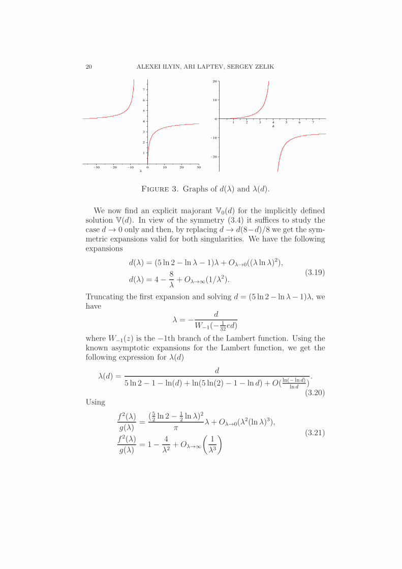
Figure 3. Graphs of d(λ) and λ(d).

We now find an explicit majorant V0(d) for the implicitly definedsolution V(d). In view of the symmetry (3.4) it suffices to study thecase d → 0 only and then, by replacing d → d(8−d)/8 we get the sym-metric expansions valid for both singularities. We have the followingexpansions

d(λ) = (5 ln 2− lnλ− 1)λ+Oλ→0((λ lnλ)2),

d(λ) = 4−8

λ+Oλ→∞(1/λ2).

(3.19)

Truncating the first expansion and solving d = (5 ln 2− lnλ− 1)λ, wehave

λ = −d

W−1(− 132ed)

where W−1(z) is the −1th branch of the Lambert function. Using theknown asymptotic expansions for the Lambert function, we get thefollowing expression for λ(d)

λ(d) =d

5 ln 2− 1− ln(d) + ln(5 ln(2)− 1− ln d) +O( ln(− lnd)lnd )

.

(3.20)Using

f 2(λ)

g(λ)=

(52 ln 2−12 lnλ)

2

πλ+Oλ→0(λ

2(lnλ)3),

f 2(λ)

g(λ)= 1−

4

λ2+Oλ→∞

(1

λ3

) (3.21)


and substituting (3.20) into the first expansion we get

V(d) =1

4πd(− ln d+ ln(1− ln d) + γ + od→0(1))

where γ = 5 ln(2) + 1 < 2π. This justifies our choice of the approxi-mation to V(d):

V0(d) =1

4π

d(8− d)

8

(ln

16

d(8− d)+ ln

(1 + ln

16

d(8− d)

)+ 2π

)

The constant 2π instead of γ (and the numerator 16) are chosen sothat for d = 4 we have V(4) = V0(4) = 1.The asymptotic expansion of V0(d) at d = 0 shows that V(d) <

V0(d) for 0 < d ≤ d0, where d0 is sufficiently small.Using the expansions at λ = ∞ in (3.19) and (3.21) we find that

V(d) = 1−(4− d)2

16+Od→4((4− d)3).

Since

V0(d) = 1−(1−

1

π

)(4− d)2

16+Od→4((4− d)3),

it follows that V(d) ≤ V0(d) for d ∈ [4 − d1, 4] for a small d1 >0. Corresponding to [d0, d1] is the finite interval [λ0,λ1] on whichcomputer calculations show that the inequality V(d) ≤ V0(d) stillholds. This gives that

V(d) ≤ V0(d)

for all d ∈ [0, 4] and hence, by symmetry, for d ∈ [0, 8].Thus, we have proved the following inequality.

Theorem 3.3. For u ∈ l2(Z2)

u(0, 0)2 ≤1

4π

∥∇u∥2

∥u∥2

(1−

∥∇u∥2

8∥u∥2

)⎛

⎝ln16

∥∇u∥2

∥u∥2

(8− ∥∇u∥2

∥u∥2

)+

+ ln

⎛

⎝1 + ln16

∥∇u∥2

∥u∥2

(8− ∥∇u∥2

∥u∥2

)

⎞

⎠+ 2π

⎞

⎠ , (3.22)

where the constants in front of logarithms and 2π are sharp. Theinequality saturates for u = δ, otherwise the inequality is strict.


4. 3D case

In the three-dimensional case the following result holds which issomewhat similar to the classical Sobolev inequality for the limitingexponent.

Theorem 4.1. Let u ∈ l2(Z3). Then for any θ ∈ [0, 1]

u(0, 0, 0)2 ≤ K3(θ)∥u∥2θ∥∇u∥2(1−θ), (4.1)

where K3(θ) < ∞ for θ ∈ [0, 1], and its sharp value for θ ∈ (0, 1) isgiven by

K3(θ) =1

2π2

1

θθ(1− θ)1−θmaxλ>0

λθ

∫ π

0

K(

1λ4+1+sin2 x

2

)

λ4 + 1 + sin2 x

2

dx, (4.2)

and there exists a unique extremal element, which belongs to l2(Z3).In the limiting case θ = 0 inequality (4.1) still holds:

u(0, 0, 0)2 ≤ K3(0)∥∇u∥2, (4.3)

where

K3(0) =1

(2π)3

∫

T3

dx

4(sin2 x12 + sin2 x2

2 + sin2 x32 )

=

=1

2π2·∫ π

0

K(

11+sin2 x

2

)

1 + sin2 x2

dx =4.9887 . . .

2π2= 0.2527 . . . .

(4.4)

The constant is sharp and there exists a unique extremal element,which does not lie in l2(Z3), but rather in l∞0 (Z3), but whose gradientdoes belong to l2(Z3). Furthermore, as we already mentioned in §1,we have the closed form formula for K3(0) (see [3])

K3(0) =

√6

24(2π)3Γ( 1

24)Γ(524)Γ(

724)Γ(

1124).

Proof. We have to find the fundamental solution Gλ(k, l,m) of theequation

A(λ)Gλ = (D∗1D1 +D∗

2D2 +D∗3D3 + λ)Gλ = δ. (4.5)

Similarly to the 1D and 2D cases we find that the function

gλ(x, y, z) :=∞∑

k,l,m=−∞

Gλ(k, l,m)eikx+ily+imz,


0 0.2 0.4 0.6 0.8 10.2

0.3

0.4

0.5

0.6

0.7

0.8

0.9

1

0 0.02 0.04 0.06 0.08 0.1 0.12 0.14 0.16

0.23

0.235

0.24

0.245

0.25

0.255

0.26

0.265

0.27

Figure 4. Graph of K3(θ) on the interval θ ∈ [0, 1](left)with a closer look at its behavior near θ = 0 (right).

satisfies

gλ(x, y, z) =14

λ4 + sin2 x

2 + sin2 y2 + sin2 z

2

.

As before we have the inequality

u(0, 0, 0)2 ≤ Gλ(0, 0, 0)(∥∇u∥2 + λ∥u∥2), (4.6)

which saturates for u = const ·Gλ.For λ > 0 as in the 1D and 2D cases we have gλ ∈ L2(T3), and,

hence, Gλ ∈ l2(Z3) for λ > 0. In particular, using (3.10) we find

Gλ(0, 0, 0) =1

8π3

∫ π

−π

∫ π

−π

∫ π

−π

gλ(x, y, z)dxdydz =

=1

2π2

∫ π

0

K(

1λ4+1+sin2 x

2

)

λ4 + 1 + sin2 x

2

dx.

(4.7)

However, unlike the previous two cases, now gλ is integrable for allλ ≥ 0 including λ = 0: gλ ∈ L1(T3) for λ ≥ 0. Therefore the Green’sfunction G0 is well defined and belongs to l∞0 (Z3). We point out,however, that since g0 /∈ L2(T3), it follows that G0 /∈ l2(Z3).For λ = 0, the integrand has only a logarithmic singularity at x = 0

and we obtain

G0(0, 0, 0) =1

2π2

∫ π

0

K(

11+sin2 x

2

)

1 + sin2 x2

dx.


We now see that f(λ) := Gλ(0, 0, 0) is continuous on λ ∈ [0,∞) and isof the order 1/λ at infinity. This gives that for θ ∈ (0, 1) the functionλθf(λ) vanishes both at the origin and at infinity. Hence, it attainsits maximum at a (generically) unique point λ∗(θ), and the claim ofthe theorem concerning the case θ ∈ (0, 1) follows in exactly the sameway as in Theorem 2.2.Setting λ = 0 in (4.6) we obtain (4.3) with (4.4). It remains to

verify that ∇G0 ∈ l2(Z3). To see this we use notation (2.11) andLemma 2.1. We obtain

∥∇Gλ∥2 = h(λ) = f(λ) + λf ′(λ) =

=1

8π3

∫ π

−π

∫ π

−π

∫ π

−π

(gλ(x, y, z) + λgλ(x, y, z)′λ)dxdydz =

=1

8π3

∫ π

−π

∫ π

−π

∫ π

−π

14(sin

2 x2 + sin2 y

2 + sin2 z2)

(λ4 + sin2 x2 + sin2 y

2 + sin2 z2)

2dxdydz.

Since the integral on right-hand side is bounded for λ = 0 we have∥∇G0∥2 < ∞. Finally, Gλ has strictly positive elements for λ ≥ 0,since we have as before the maximum principle. In the case when λ = 0we use, in addition, the fact that G0 ∈ l∞0 . The proof is complete. !

The graph of K3(θ) is shown in Fig. 4.

Remark 4.1. Higher dimensional cases are treated similarly, in par-ticular, for d ≥ 3 and θ = 0

u(0)2 ≤ Kd(0)∥∇u∥2, Kd(0) =1

(2π)d

∫

Td

dx

4(sin2 x12 + · · ·+ sin2 xd

2 ).

(4.8)In §6 we give an independent elementary proof of this inequality.

5. Higher order difference operators

The method developed above admits a straight forward generaliza-tion to higher order difference operators. We consider the second-orderoperator in the one dimensional case:

u(0)2 ≤ K1,2(θ)∥u∥2θ∥∆u∥2(1−θ), (5.1)

where

−∆u(n) := D∗Du(n) = −(u(n+ 1)− 2u(n) + u(n− 1)

).


Accordingly, the operator A(λ) is

A(λ) =

∆2 + λ, for λ > 0;

−∆2 − λ, for λ < −16.(5.2)

Here

∆2u(n) = u(n+ 2)− 4u(n+ 1) + 6u(n)− 4u(n− 1) + u(n− 2).

As before, we have to find the Green’s functionGλ solving A(λ)Gλ = δ.Furthermore, for finding K1,2(θ) it suffices to solve this equation forλ > 0. Setting

gλ(x) :=∞∑

n=−∞

Gλ(n)einx,

and arguing as in Lemma 2.2 we get from (5.2)

1 = gλ(x)(λ+ e−i2x − 4e−ix + 6− 4eix + ei2x) =

= gλ(x)(λ+ (eix/2 − e−ix/2)4

)= gλ(x)

(λ+ 16 sin4 x

2

),

(5.3)

so that

Gλ(0) =1

2π

∫ π

−π

dx

λ+ 16 sin4 x2

=

√2

2

1

λ3/4

√√λ+ 16 +

√λ

λ+ 16. (5.4)

Now a word for word repetition of the argument in Theorem 2.2 givesthat

K1,2(θ) =1


λθGλ(0).

Therefore we see from (5.4) that K1,2(θ) < ∞ if and only if

3

4≤ θ ≤ 1.

For example, for θ = 3/4 supremum is the maximum attained atλ∗(3/4) = 16/3, giving

K1,2(3/4) =4

33/4· λ3/4Gλ(0)|λ∗(3/4)= 16

3=

√2

2.

We only mention that in the general case

λ∗(θ) = argmaxλ>0 λθ−3/4

√√λ+ 16 +

√λ

λ+ 16=

=64θ − 32θ2 − 29 +

√32θ − 23

2θ2 − 5θ + 3,

(5.5)


however, the corresponding substitution produces a long (but explicit)formula for K1,2(θ), and instead we present in Fig.5 the graph of thesharp constant K1,2(θ), where K1,2(3/4) =

√2/2 and K1,2(1) = 1.

Figure 5. Graph of K1,2(θ) on θ ∈ [3/4, 1].

Finally, it is possible to find Gλ(n) explicitly. In fact, the freerecurrence relation ∆2Gλ + λGλ = 0 has the characteristic equation

q2 − 4q + (6 + λ)− 4q−1 + q−2 = 0,

or (q1/2 − q−1/2)4 = −λ, which decomposes into two quadratic equa-tions

q +1

q− 2 = i

√λ and q +

1

q− 2 = −i

√λ,

with four roots q1, q2, q3, q4, where q2 = 1/q1, q3 = q2, q4 = q1, where

q1 = q(λ) = 1−λ1/4

√√λ+ 16−

√λ

2√2

+i

(√λ

2−

λ1/4√√

λ+ 16 +√λ

2√2

)

.

(5.6)Since |q(λ)| < 1 for λ > 0, it follows that any symmetric l2-solutionof (5.2) is of the form a(λ)q(λ)|n| + b(λ)q(λ)|n|, and since, in additionGλ(n) is real, we have

Gλ(n) = a(λ)q(λ)|n| + a(λ)q(λ)|n|.

Setting n = 0 and n = 1 we obtain a linear system for a(λ)

Gλ(0) = 2Re a(λ)

Gλ(1) = a(λ)q(λ) + a(λ)q(λ),


where Gλ(0) is given in (5.4) and

Gλ(1) =1

π

∫ π

0

cosx dx

λ+ 16 sin4 x2

=

√2

2

1

λ3/4

√λ+ 16−

√λ√√

λ+ 16 +√λ√λ+ 16

.

Solving this system we find a(λ):

a(λ) =

√2

4

1

λ3/4√λ+ 16

√√λ+ 16 +

√λ

(√λ+ 16 +

√λ+ 4i

),

and, consequently, the formula for Gλ(n) with λ > 0:

Gλ(n) =1

π

∫ π

0

cosnx dx

λ+ 16 sin4 x2

=Re[(√

λ+ 16 +√λ+ 4i

)· q(λ)|n|

]

√2λ3/4

√λ+ 16

√√λ+ 16 +

√λ

,

(5.7)where q(λ) is given in (5.6).

Figure 6. Graph of the maximizer G 163(n) for n ∈ [0, 6]

(left) and n ∈ [6, 12] (right)

Thus, we obtain the following result.

Theorem 5.1. Inequality (5.1) holds for θ ∈ [3/4, 1]. In particular,in the limiting case θ = 3/4

u(0)2 ≤√2

2∥u∥3/2∥∆u∥1/2. (5.8)

In the general case,

K1,2(θ) =1

θθ(1− θ)1−θ· λ∗(θ)

θGλ∗(θ)(0),


where λ∗(θ) is given in (5.5) and Gλ(0) in (5.4) (see also (5.7)). Forθ ∈ [3/4, 1) the unique extremal is uλ∗(θ) = Gλ∗(θ). For θ = 1, λ∗(1) =∞ and u∗ = δ.

Remark 5.1. It is not difficult to find the function V(d), that is, thesolution of the maximization problem

V(d) := supu(0)2 : u ∈ l2(Z), ∥u∥2 = 1, ∥∆u∥2 = d

, (5.9)

where d ∈ [0, 16]. For this purpose we also need the expression for theGreen’s function Gλ(0) in the region λ ≤ −16, which is as follows

Gλ(0) = −1

2π

∫ π

−π

dx

λ+ 16 sin4 x2

=1

2(−λ)3/4

√√−λ+ 4 +

√√−λ− 4√

−λ− 16.

(5.10)Using (5.4), (5.10) we can write down a parametric representation ofV(d) as in Theorem 3.2, but instead we merely show its graph in Fig.7.

Figure 7. Graph of V(d) defined in (5.9).

This time we do not have the maximum principle, and the Green’sfunction Gλ(n) is not positive for all n, but is rather oscillating withexponentially decaying amplitude, see Fig. 6. Nor do we have thesymmetry V(d) = V(16 − d) in Fig. 7 that we have seen in the first-order inequalities in the one- and two-dimensional cases, see (2.8) and(3.4). The maximum is attained at d = 6 corresponding to u = δ. Thecomponent λ ∈ (0,∞) of the resolvent set corresponds to d ∈ (0, 6)and λ ∈ (−∞,−16) corresponds to d ∈ (6, 16).

It is worth to compare the results so obtained in the discrete casewith the corresponding interpolation inequalities for Sobolev spaces in


the continuous case. It is well known that the interpolation inequalityon the whole line R

∥f∥2L∞≤ C1,n(θ)∥f∥2θ∥f (n)∥2(1−θ), (5.11)

where f ∈ Hn(R), holds only for θ = 1− 12n . The sharp constant was

found in [17]:

C1,n(θ) =1

θθ(1− θ)1−θ

1

π

∫ ∞

0

dx

1 + x2n=

1

θθ(1− θ)1−θ

1

2n

1

sin π2n

.

(5.12)Thus, for first-order inequalities both in the discrete and contin-

uous cases the constants are equal to 1, while for the second-orderinequalities we see from (5.8) and (5.12) that

C1,2(3/4) =

(4

27

)1/4

<

√2

2= K1,2(3/4).

The next theorem states that for higher order inequalities the con-stants in the discrete case are always strictly greater than those in thecontinuous case.

Theorem 5.2. Let n ≥ 1 and let u ∈ l2(Z). The inequality

u(0)2 ≤ K1,n(θ)∥u∥2θ∥Dnu∥2(1−θ), (5.13)

where

Dn :=

∆n/2, for n even,∇∆(n−1)/2, for n odd,

(5.14)

holds for θ ∈ [1− 1/(2n), 1] and

K1,n(θ) =1

θθ(1− θ)1−θ

1

πsupλ>0

λθ

∫ π

0

dx

λ+ 22n sin2n x2

. (5.15)

For all θ ∈ [1− 1/(2n), 1] supremum is the maximum. If n ≥ 2, thenfor θ = θ∗ := 1 − 1/(2n) the constants in the continuous and discreteinequalities satisfy

C1,n(θ∗) < K1,n(θ∗). (5.16)

Proof. Following the scheme developed above we look for the solutionof the equation

(−1)n∆nGλ + λGλ = δ,

and as in (5.3) find that

Gλ(0) =1

π

∫ π

0

dx

λ+ 22n sin2n x2

,


which proves (5.15) (whenever the supremum is finite). Using sin2 x2 =

tan2 x2/(1 + tan2 x

2 ) and changing the variable tan x2 =

√µt, where

µ = λ1/n we have

λθ∗

∫ π

0

dx

λ+ 22n sin2n x2

=

∫ ∞

0

2dt

(1 + µt2)(1 + 22nt2n

(1+µt2)n )=: S(µ).

Clearly S(∞) = 0, and we have to study S(µ) as µ → 0. The integralconverges uniformly for µ ∈ [0, 1], since the denominator is greaterthen 1 for t ∈ [0, 1] and is greater then 1 + c(n)t2 for t ≥ 1 observingthat t2n/(1 + µt2)n−1 ≥ c1(n)t2 uniformly for µ ∈ [0, 1]. Therefore

limµ→0

S(µ) = S(0) =

∫ ∞

0

2dt

1 + 22nt2n=

∫ ∞

0

dx

1 + x2n,

which proves, in the first place, that the right-hand side in (5.15) isfinite if and only if θ ∈ [θ∗, 1] and, secondly, that non-strict inequality(5.16) holds. Finally, for n ≥ 2 we have strict inequality since

S ′µ(0) = 2

∫ ∞

0

[n22nt2n+2

(1 + 22nt2n)2−

t2

1 + 22nt2n

]dt =

1

16n

π

sin 3π2n

> 0.

For n = 1 we have λ = µ, S ′µ(0) < 0 and

S(µ) =π√µ+ 4

is strictly decreasing not only at µ = 0 but for all µ ≥ 0, the fact thatwe have already seen in (2.24). !

Remark 5.2. Inequality (5.13) holds for θ ∈ [1 − 1/(2n), 1], that is,when the weight of the stronger norm, which is the l2-norm, increases.Accordingly, inequality (5.11) for periodic functions with mean valuezero holds for θ in the complementary interval θ ∈ [0, 1 − 1/(2n)],when the weight of the stronger norm, which is the L2-norm of then-th derivative, increases:

∥f∥2L∞≤ Cper

1,n(θ)∥f∥2θ∥f (n)∥2(1−θ), θ ∈ [0, 1− 12n ], (5.17)

where

f ∈ Hnper(S

1),

∫ 2π

0

f(x)dx = 0.

A general method for finding sharp constants in interpolation inequal-ities of L∞-L2-L2-type was developed in [11], [1], [18], which was also


used in the discrete case in the present paper. For example, for n = 1

Cper1,1 (θ) =

1

θθ(1− θ)1−θsupλ≥0

λθG(λ), θ ∈ [0, 1/2], (5.18)

where Gλ(x, ξ) = 12π

∑x∈Z\0

eik(x−ξ)

k2+λ is the Green’s function of theequation

−Gλ(x, ξ)′′ + λGλ(x, ξ) = δ(x− ξ), x, ξ ∈ [0, 2π]per,

and

G(λ) := Gλ(ξ, ξ) =1

π

∞∑

k=1

1

k2 + λ=

1

2π

π√λ coth(π

√λ)− 1

λ.

For the limiting θ = θ∗=1/2 the constant is the same as on R:Cper

1,1 (θ∗) = C1,1(θ∗) = 1. The graph of Cper1,1 (θ) on the interval θ ∈

[0, 1/2] is shown in Fig.1 on the left. Observe that C1,1(0) = π/6.

6. Applications

Discrete and integral Carlson inequalities. We now discuss ap-plications of the inequalities for the discrete operators, and our firstgroup of results concerns Carlson inequalities. The original Carlsoninequality [5] is as follows:

(∞∑

k=1

ak

)2

≤ π

(∞∑

k=1

a2k

)1/2( ∞∑

k=1

k2a2k

)1/2

, (6.1)

where the constant π is sharp and cannot be attained at a non iden-tically zero sequence ak∞k=1. This inequality has attracted a lot ofinterest and has been a source of generalizations and improvements(see, for example, [10], [12] and the references therein, and also [18]for the most recent strengthening of (6.1)). Inequality (6.1) has anintegral analog (with the same sharp constant)

(∫ ∞

0

g(t)dt

)2

≤ π

(∫ ∞

0

g(t)2dt

)1/2(∫ ∞

0

t2g(t)2dt

)1/2

. (6.2)

As was first observed in [9], inequality (6.1) is equivalent to the in-equality

∥f∥2∞ ≤ 1 · ∥f∥∥f ′∥, (6.3)


for periodic functions f ∈ H1per(0, 2π),

∫ 2π0 f(x)dx = 0, by setting for

a sequence ak∞k=1

f(x) =∞∑

k=−∞

a|k|eikx, a0 = 0.

Accordingly, inequality (6.3) for f ∈ H1(R) is equivalent (as wasfirst probably observed in [15]) to (6.2) by setting g = Ff and furtherrestricting g (and f) to even functions. Furthermore, the unique (upto scaling) extremal function f∗(x) = e−|x| in (6.3) on the whole axisproduces the extremal function g∗(t) = 1/(1 + t2) in (6.2).In the similar way, discrete inequalities have equivalent integral

analogs. Let F be the discrete Fourier transform F : a(n) → a(x),where

a(x) =∑

n∈Zd

a(n)einx, a(n) = (2π)−d

∫

Td

a(x)e−inxdx.

Then for ej = (0, . . . , 0, 1, 0, . . . , 0) with 1 on the jth place

Dja(n) = a(n + ej)− a(n) = (2π)−d

∫

Td

a(x)(e−i(n+ej)x − e−inx)dx =

= (2π)−d

∫

Td

a(x)e−ix/2(−2i) sin xj

2 e−inxdx.

Therefore

∥Dja∥2 = (2π)−d

∫

Td

|a(x)|24 sin2 xj

2 dx. (6.4)

and, finally,

∥a∥2 = (2π)−d∥a∥2, ∥∇a∥2 = (2π)−d

∫

Td

|a(x)|24∑d

j=1sin2 xj

2 dx.

(6.5)Thus, we have proved the following result.

Theorem 6.1. Let 1/2 < θ ≤ 1. The inequality

u(0)2 ≤ K1(θ)∥u∥2θ∥Du∥2(1−θ), u ∈ l2(Z)

established in Theorem 2.2 is equivalent to the inequality(∫ 2π

0

g(x)dx

)2

≤ 2πK1(θ)

(∫ 2π

0

g(x)2dx

)θ (∫ 2π

0

4 sin2 x2 g(x)

2dx

)1−θ

,

(6.6)


for g ∈ L2(0, 2π). Here K1(θ) =12 (2/θ)

θ (2θ− 1)θ−1/2 (see (2.28)). Inthe limiting case inequality (2.27) is equivalent to

(∫ 2π

0

g(x)dx

)2

≤

π

√√√√4−∫ 2π0 4 sin2 x

2 g(x)2dx

∫ 2π

0 g(x)2dx

(∫ 2π

0

g(x)2dx

)1/2(∫ 2π

0

4 sin2 x2 g(x)

2dx

)1/2

(6.7)

Proof. The proof follows from Theorem 2.2 and (6.4). We also pointout that for θ ∈ (1/2, 1) inequality (6.6) saturates for

gλ∗(x) =

1

λ∗ + 4 sin2 x2

, λ∗ = λ∗(θ) =4θ − 2

1− θ.

for θ = 1/2 no extremals exist and maximizing sequence is obtainedby letting λ∗ → 0; finally for θ = 1, (6.6) saturates at constants.For each d, 0 < d < 4 and λ(d) = 2d

2−d inequality (6.7) saturates at

gλ(d)(x) =1

λ(d) + 4 sin2 x2

, with

∫ 2π

0 4 sin2 x2 gλ(d)(x)

2dx∫ 2π0 gλ(d)(x)2dx

= d.

For d = 2, g = const. !

Remark 6.1. Corresponding to (5.8) is the integral inequality(∫ 2π

0

g(x)dx

)2

≤ π√2

(∫ 2π

0

g(x)2dx

)3/4(∫ 2π

0

16 sin4 x2 g(x)

2dx

)1/4

,

(6.8)which turns into equality for

g∗(x) =1

163 + 16 sin4 x

2

.

Remark 6.2. The integral analog of the two dimensional discreteinequality is

(∫

T2

g(x, y)dxdy

)2

≤

(2π)2K2(θ)

(∫

T2

g(x, y)2dxdy

)θ (∫

T2

4(sin2 x2 + sin2 y

2) g(x, y)2dxdy

)1−θ

,

(6.9)where θ ∈ (0, 1], and K2(θ) is defined in (3.11).


Remark 6.3. In the d-dimensional case, d ≥ 3, for the exponent θ = 0the Parceval’s identities (6.5) provide an independent elementary proofof (4.8). In fact, setting g0(x) = 4

∑dj=1 sin

2 xj

2 we have

(2π)2d|a(0)|2 =∣∣∣∣

∫

Td

a(x)dx

∣∣∣∣2

≤

≤(∫

Td

|a(x)|g0(x)1/2g0(x)−1/2dx

)2

≤

≤∫

Td

|a(x)|2g0(x)dx∫

Td

g0(x)−1dx = (2π)2dKd(0)∥∇a∥2,

(6.10)

which proves (4.8).

This approach can be generalized to the lp-case for the proof of thediscrete Sobolev type inequality in the non-limiting case (1.12). Herein addition to the Parseval’s identity we also use the Hausdorff-Younginequality (see, for instance, [2]):

∥a∥Lp(Td) ≤ (2π)d/p∥a∥lp′(Zd), (6.11)

where p ≥ 2 and p′ = p/(p− 1).In fact, we have ∥F∥l2→L2 = (2π)d/2 and ∥F∥l1→L∞

= 1 and by theRiesz–Thorin interpolation theorem

∥F∥lp′→Lp≤ (2π)dθ/2 = (2π)d/p,

where 1p′ =

θ2 +

1−θ1 , 1

p = θ2 +

1−θ∞ . We also observe that (6.11) becomes

an equality for a(x) = 1 and a = δ.Setting q = 2p in (1.12), v(n) := u(n)pu(n)p−1, and using the aux-

iliary inequality (6.12), (6.13) below, we obtain

∥u∥2pl2p =∑

n∈Zd

v(n)u(n) =∑

n∈Zd

(D∗D∆−1v(n))u(n) =

=∑

n∈Zd

D∆−1v(n)Du(n) ≤

(∑

n∈Zd

|D∆−1v(n)|2)1/2

∥Du∥ ≤

≤(1

4(2π)d/p

′

Ip′,d

)1/2

∥v∥l(2p)′∥Du∥ =

(1

4(2π)d/p

′

Ip′,d

)1/2

∥u∥2p−1l2p ∥Du∥.


It remains to prove (6.12). By Holder’s inequality and (6.11) we have

∑

n∈Zd

|D∆−1v(n)|2 =(2π)d

4

∫

Td

|v(x)|2dx∑d

j=1 sin2 xj

2

≤

≤(2π)d

4Ip′,d

(∫

Td

|v(x)|2pdx)1/p

≤

≤(2π)d

4Ip′,d(2π)

d/p∥v∥2l(2p)′

=1

4(2π)d(p+1)/pIp′,d∥v∥2l(2p)′

(6.12)

where

Ip′,d =

(∫

Td

dx

(∑d

j=1 sin2 xj

2 )p′

)1/p′

< ∞ for p′ < d/2 ⇔ p > d/(d− 2).

(6.13)Thus we obtain the following result.

Theorem 6.2. Let d ≥ 3 and 2p > 2d/(d− 2). Then

∥u∥2l2p(Z)d =

(∑

n∈Zd

|u(n)|2p)1/p

≤1

4(2π)d(p+1)/pIp′,d∥Du∥2,

where Ip′,d is defined in (6.13).

Remark 6.4. We do not claim that the constant here is sharp. More-over, it blows up for 2p = 2d/(d− 2), while it can be shown that theinequality still holds. However, the constant is sharp in the oppositelimit p = ∞, see (4.8).

Spectral inequalities for discrete operators. Interpolation in-equalities characterizing imbeddings of Sobolev spaces into the spaceof bounded continuous functions have important applications in spec-tral theory. The original fruitful idea in [7] has been generalized in [6]to give best-known estimates for the Lieb–Thirring constants in esti-mates for the negative trace of Schrodinger operators.In this section we apply our sharp interpolation inequalities with

the method of [7] for estimates of the negative trace of the discreteoperators [16].We write the inequalities obtained above in the unform way

supk∈Zd

u(k)2 ≤ K(θ)∥u∥2θ∥Dnu∥2(1−θ), (6.14)


where Dn is as in (5.14) and θ belongs to a certain subinterval of [0, 1]uniquely defined in the corresponding theorem:

θ ∈

⎧⎨

⎩

[1-1/(2n),1], d = 1, n ≥ 1;(0, 1], d = 2, n = 1;[0, 1], d ≥ 3, n = 1.

(6.15)

Theorem 6.3. Let u(j)Nj=1 ∈ l2(Zd) be a family of N sequences thatare orthonormal with respect to the natural scalar product in l2(Zd).We set

ρ(k) :=N∑

j=1

u(j)(k)2, k ∈ Zd. (6.16)

Then for θ as in (6.15) and θ < 1

∥ρ∥2−θ1−θ

l2−θ1−θ

=∑

k∈Zd

ρ(k)2−θ1−θ ≤ K(θ)

11−θ

N∑

j=1

∥Dnu(j)∥2. (6.17)

Proof. For arbitrary ξ1, . . . , ξN ∈ R we construct a sequence f ∈ l2(Zd)

f(k) :=N∑

j=1

ξju(j)(k), k ∈ Z

d.

Applying (6.14) and using orthonormality we obtain for a fixed k

f(k)2 ≤ K(θ)

(N∑

j=1

ξ2j

)θ( N∑

i,j=1

ξiξj(Dnu(i),Dnu(j)

))1−θ

.

We now set ξj := u(j)(k):

ρ(k)2 ≤ K(θ)ρ(k)θ(

N∑

i,j=1

u(i)(k)u(j)(k)(Dnu(i),Dnu(j)

))1−θ

,

or

ρ(k)2−θ1−θ ≤ K(θ)

11−θ

N∑

i,j=1

u(i)(k)u(j)(k)(Dnu(i),Dnu(j)

).

Summing over k ∈ Zd and using orthonormality we obtain (6.17). !

Corollary 6.1. Setting N = 1 in Theorem 6.3 we obtain a family ofinterpolation inequalities for u ∈ l2(Zd)

∥u∥l2(2−θ)1−θ (Zd)

≤ K(θ)1

2(2−θ) ∥u∥1

2−θ ∥Dnu∥1−θ2−θ . (6.18)


In particular, to mention a few examples with limiting θ

∥u∥l6(Z) ≤ 1 · ∥u∥2/3∥Du∥1/3, θ = 1/2,

∥u∥l10(Z) ≤ 2−1/5 ∥u∥4/5∥∆u∥1/5, θ = 3/4,

in dimension d ≥ 3

∥u∥l4(Zd) ≤ Kd(0)1/4∥u∥1/2∥∇u∥1/2, θ = 0.

Remark 6.5. The last inequality holding in dimesion three and highercuriously resembles the celebrated Ladyzhenskaya inequality that isvital for the uniqueness of the weak solutions of the two-dimensionalNavier–Stokes system:

∥f∥L4(Ω) ≤ cL∥f∥1/2∥∇f∥1/2, f ∈ H10 (Ω), Ω ⊆ R

2.

We now exploit the equivalence between the inequalities for or-thonormal families and spectral estimates for the negative trace ofthe Schrodinger operators [14].We consider the discrete Schrodinger operator

H := (−1)n∆n − V, (6.19)

acting on u ∈ l2(Zd) as follows

Hu(k) = (−1)n∆nu(k)− V (k)u(k).

Theorem 6.4. Let V (k) ≥ 0 and let V (k) → 0 as |k| → ∞, then thenegative spectrum of H is discrete and satisfies the estimate

∑|λj| ≤ K(θ)

(1− θ)1−θ

(2− θ)2−θ

∑

k∈Zd

V (k)2−θ. (6.20)

Proof. Suppose that there exists N negative eigenvalues −λj < 0,j = 1, . . . , N with corresponding N orthonormal eigenfunctions u(j):

(−1)n∆nu(j)(k)− V (k)u(j)(k) = −λju(j)(k).


Taking the scalar product with u(j), summing the the results withrespect to j, and using (6.16), Holder inequality and (6.17), we obtain

N∑

j=1

λj = (V, ρ)−N∑

j=1

∥Dnu(j)∥2 ≤

∥V ∥l2−θ∥ρ∥l 2−θ

1−θ

−K(θ)−1

1−θ ∥ρ∥2−θ1−θ

l 2−θ1−θ

≤

maxy>0

(∥V ∥l2−θ

y −K(θ)−1

1−θ y2−θ1−θ

)=

K(θ)(1− θ)1−θ

(2− θ)2−θ

∑

k∈Zd

V (k)2−θ.

!

Examples.d = 1, n = 1, θ = 1/2. Then K = 1 and the negative trace of theoperator

−∆− V in l2(Z)

satisfies∑

|λj| ≤2

3√3

∞∑

α=−∞

V 3/2(α).

d = 1, n = 2, θ = 3/4. Then K =√2/2 and the negative trace of the

operator∆2 − V in l2(Z)

satisfies∑

|λj| ≤2√2

55/4

∞∑

α=−∞

V 5/4(α).

d ≥ 3, n = 1, θ = 0. Then K = Kd(0) and the negative trace of theoperator

−∆− V in l2(Zd)

satisfies∑

|λj| ≤Kd(0)

4

∑

α∈Zd

V 2(α).

In particular, in three dimensions

K3(0)

4= 0.0631 . . . .


Acknowledgements. Funding for this research was provided by thegrant of the Russian Federation Government to support scientific re-search under the supervision of leading scientist at Siberian FederalUniversity, 14.Y26.31.0006, and from the Russian Foundation for Ba-sic Research (grant no. 12-01-00203).

References

1. M.V. Bartuccelli, J. Deane, and S.V. Zelik, Asymptotic expansions and ex-tremals for the critical Sobolev and Gagliardo-Nirenberg inequalities on atorus. Proceedings of the Royal Society of Edinburgh 143A (2013), 445–482.

2. J. Bergh, J. Lofstrom. Interpolation spaces. An introduction. Grundlehren derMathematischen Wissenschaften, No. 223. Springer–Verlag, Berlin–New York,1976.

3. J. M. Borwein, M. L. Glasser, R. C. McPhedran, J. G. Wan, and I. J. Zucker.Lattice Sums Then and Now. Encyclopedia of mathematics and its applications150. Cambridge University Press, Cambridge, 2013.

4. H. Brezis and T. Gallouet. Nonlinear Schrodinger evolution equations. Non-linear Anal. 4 (1980), 677-681.

5. F. Carlson, Une inegalite, Ark. Mat. Astr. Fysik 25B (1934), No. 1.6. J. Dolbeault, A. Laptev, and M.Loss, Lieb–Thirring inequalities with im-

proved constants. J. European Math. Soc. 10:4 (2008), 1121–1126.7. A. Eden and C. Foias, A simple proof of the generalized Lieb–Thirring in-

equalities in one space dimension. J. Math. Anal. Appl. 162 (1991), 250–254.8. I.S.Gradshteyn and I.M.Ryzhik, Table of Integrals, Series and Products. Aca-

demic Press, London, 2007.9. G.H. Hardy, A note on two inequalities. J. London Math. Soc. 11 (1936), 167–

170.10. G.H. Hardy, J.E. Littlewood, and G.Polya. Inequalities, Cambridge Univ.

Press, Cambridge 1934; Addendum by V.I. Levin and S.B. Stechkin to theRussian translation, GIIL, Moscow 1948; English transl. in V.I. Levin andS.B. Stechkin, Inequalities, Amer. Math. Soc. Transl., 14 (1960), 1-22.

11. A.A. Ilyin, Best constants in multiplicative inequalities for sup-norms. J. Lon-don Math. Soc.(2) 58, 84–96 (1998).

12. L. Larsson, L.Maligranda, J.Pecaric, L.–E.Persson, Multiplicative inequalitiesof Carlson type and intepolation. World Scientific, Singapore, 2006.

13. A. Laptev and T.Weidl, Sharp Lieb–Thirring inequalities in high dimensions.Acta Math. 184 (2000), 87–111.

14. E. Lieb and W.Thirring, Inequalities for the moments of the eigenvalues ofthe Schrodinger Hamiltonian and their relation to Sobolev inequalities, Studiesin Mathematical Physics. Essays in honor of Valentine Bargmann, PrincetonUniversity Press, Princeton NJ, 269–303 (1976).

15. B. Sz.-Nagy, Uber integralungleichungen zwischen einer funktion und ihrerableitung. Acta Univ. Szeged, Sect. Sci. Math. 10 (1941), 64–74.


16. A. Sahovic, New constants in discrete Lieb-Thirring inequalities for Jacobimatrices. Problems in mathematical analysis. No. 45. J. Math. Sci. (N. Y.)166:3 (2010), 319-327.

17. L.V.Taikov, Kolmogorov-type inequalities and the best formulas for numericaldifferentiation. Mat. Zametki 4, 233–238 (1968); English transl. Math. Notes4 (1968), 631–634.

18. S.V. Zelik, A.A.Ilyin. Green’s function asymptotics and sharp interpolationinequalities. Uspekhi Mat. Nauk 69:2 (2014), 23–76; English transl. in RussianMath. Surveys 69:2 (2014).

Keldysh Institute of Applied Mathematics and Institute for Infor-mation Transmission Problems;Imperial College London and Institute Mittag–Leffler;University of Surrey, Department of Mathematics and Keldysh In-stitute of Applied Mathematics

E-mail address : [email protected]; [email protected];

[email protected]

sharp interpolation inequalities for discrete operators ...alaptev/papers/ilz.pdf · sharp...

Documents