Shear-Sensitive Polymer Dispersed Liquid Crystal

Guo Shi Li

A thesis

Submitted in partial fulfillment of the

requirements for the degree of

Master of Science in Aeronautics and Astronautics

University of Washington

2012

Committee:

Dana Dabiri, Chair

Gamal Khalil

Program Authorized to Offer Degree:

Aeronautics and Astronautics

II

University of Washington

Abstract

Shear-Sensitive Polymer Dispersed Liquid Crystal

Guo Shi Li

Chair of the Supervisory Committee:

Dana Dabiri

Department of Aeronautics and Astronautics

Polymer dispersed liquid crystal has been developed as a shear stress sensor, showing a

great signal-to-noise ratio with a high temporal bandwidth. Traditional shear sensing

liquid crystal techniques are known to be irreversible processes under practical test

conditions. The introduction of polymer into the liquid crystal gives the shear-sensor an

additional temporal bandwidth that can be utilized for detecting unsteady flow

phenomena. Exploiting a revolutionary dynamic birefringence detecting system known

as “Milliview”, a series of liquid crystal polymer combinations were tested in a wind

tunnel apparatus. The signal strength and the reversibility of the tested combinations are

summarized in this paper. The preliminary results showed promising potential in this

new sensor system. It demonstrated the capability of the sensor in commercial wind

tunnel applications. The dynamic range and the bandwidth of the sensor can be adjusted

to fit different application needs. Few combinations presented qualities both in high

dynamic range and in broad bandwidth, making them ideal broad purpose sensors.

Table of Contents List of Figures ................................................................................................................................. iii

Acknowledgements ......................................................................................................................... iv

Chapter 1. Introduction ............................................................................................................. 1

1.1 Shear stress measurement ...................................................................................................... 1

1.1.1 MEMS based technologies ............................................................................................. 1

1.1.2 Thin oil film .................................................................................................................... 6

1.1.3 Liquid crystal .................................................................................................................. 8

1.2 Shear-Sensitive Polymer Dispersed Liquid Crystal .............................................................. 9

1.3 Imaging polarimetry system ................................................................................................ 11

1.4 Objectives ............................................................................................................................ 15

1.4.1 Wind tunnel applicable ................................................................................................. 15

1.4.2 Uniform and high signal-to-noise ratio ........................................................................ 15

1.4.3 Macro scale imaging with high resolution ................................................................... 15

Chapter 2. Experimental facilities, instrumentation and set up ............................................... 17

2.1 Calibration facilities ............................................................................................................ 17

2.2 Calibration set up and technique ......................................................................................... 19

2.3 Data analysis ........................................................................................................................ 21

Chapter 3. Results ................................................................................................................... 24

3.1 Initial assessment ................................................................................................................. 24

3.2 Air brushing study ............................................................................................................... 27

3.3 Poly(methyl methacrylate) study ......................................................................................... 30

3.4 Application methods study with PMMA ............................................................................. 32

3.5 Direct deposition study ........................................................................................................ 33

3.6 E7 study ............................................................................................................................... 34

3.7 Reproducibility test ............................................................................................................. 36

Chapter 4. Future works .......................................................................................................... 37

4.1 Uniformity improvement ..................................................................................................... 37

4.2 Response time study ............................................................................................................ 37

4.3 Liquid crystal alignment ...................................................................................................... 37

4.4 Reflective method ................................................................................................................ 38

4.5 Curved surface measurement .............................................................................................. 38

ii

4.6 Calibration against analytical solution ................................................................................ 38

4.7 Adding pressure sensitive paint (PSP) ................................................................................ 39

Chapter 5. Conclusion ............................................................................................................. 40

Chapter 6. References ............................................................................................................. 41

Appendix A ...................................................................................................................................... I

Appendix B...................................................................................................................................... V

Appendix C..................................................................................................................................... VI

iii

List of Figures

Figure 1.1 Schematic of a typical floating point. ............................................................................ 2

Figure 1.2 Schematic of the optical shutter design. ......................................................................... 3

Figure 1.3 Interference pattern produced by Fizeau Interferomery. ................................................ 6

Figure 1.4 Sub-states of liquid crystal. ............................................................................................ 8

Figure 1.5 PDLC under shear stress. ............................................................................................. 10

Figure 1.6 Elliptically polarized light. ........................................................................................... 11

Figure 1.7 Functional Groups of Quad-View. ............................................................................... 14

Figure 1.8 Optical components of “MilliView”. ........................................................................... 14

Figure 2.1 Experimental Apparatus. .............................................................................................. 17

Figure 2.2 Calibration facilities. .................................................................................................... 18

Figure 2.3 Calibration facilities: testing chamber. ........................................................................ 19

Figure 2.4 MilliView interface. ..................................................................................................... 20

Figure 2.5 MilliView interface (2).. .............................................................................................. 20

Figure 2.6 Shear stress versus distance at 13 MPH. ...................................................................... 22

Figure 2.7 Signal Velocity Profile. ................................................................................................ 23

Figure 3.1 Polycarbonate-Silicone Copolymer 1-1 NCU 192. ...................................................... 24

Figure 3.2 Polycarbonate-Silicone Copolymer 1-1 E7. ................................................................. 25

Figure 3.3 PBA 1-1 E7. ................................................................................................................. 25

Figure 3.4 PBMA 1-1 NCU 192. ................................................................................................... 26

Figure 3.5 PBA 1-1 NCU 192. ...................................................................................................... 26

Figure 3.6 PBMA 1-1 E7............................................................................................................... 27

Figure 3.7 PBA NCU-192 Non-revived ........................................................................................ 28

Figure 3.8 PBA NCU-192 Revived ............................................................................................... 29

Figure 3.9 MAX NCU-192 Non-revived ...................................................................................... 29

Figure 3.10 MAX NCU-192 Revived ........................................................................................... 30

Figure 3.11 PMMA 1-1 E7. ........................................................................................................... 31

Figure 3.12 Application methods study. ........................................................................................ 33

Figure 3.13 Direct deposit study. .................................................................................................. 34

Figure 3.14 E7 Study. .................................................................................................................... 35

Figure 3.15 Reproducibility test. ................................................................................................... 36

iv

Acknowledgements

First and foremost, the author wishes to express his deepest gratitude to his family

for their love and support. The author would like to express his most sincere appreciation

to Professor Dana Dabiri, Professor Gamal Khalil and Professor Werner Kaminsky for

their guidance and support throughout the course of his Master of Science degree. The

author also thanks Dr John West of Kent State University for his advice on the project.

A special thank also gives to Kenneth Low for his dedicated assistance on the

project. The author wishes to thank Viggo Hansen for his help on the project and the

equipment donated. Thanks are also given to Alex Perez, Wei-Hsin Tien, Kristina Wang

and Trenton West for their friendship and daily support. The author also wishes to thank

for the technical support received from Aeronautics & Astronautics Engineering as well

as Mechanical Engineering machine shops, namely, Dzung Tran, Dennis Peterson,

Eamon McQuaide and Kevin Soderlund. The same kind of gratitude goes towards Robert

Gordon.

,

1

Chapter 1. Introduction

Friction induced by air flowing over aerodynamic surfaces is a fundamental force

that theoretical and experimental aerodynamicists aim to calculate and measure. This

force, also known as shear stress, has traditionally been measured point-by-point across

surfaces, a process that can be both expensive and time consuming. The resolution of the

shear stress maps is dependent upon the number of points taken across the surface. To

improve upon this technology, a novel method for obtaining high-resolution, 2-

dimensional shear stress measurements over aerodynamic surfaces is proposed. The

method is based upon dynamic birefringence measurements of a shear sensitive, liquid

crystal coating. Promising to produce a robust, non-intrusive, and real-time shear stress

measuring technique, this method can be utilized on any aerodynamic surface. In this

chapter we will review some of the current methods for measuring shear stress and will

provide a brief description for the proposed technique.

1.1 Shear stress measurement Shear stress and pressure are the two predominant sources of force that act on any

aerodynamic surface. While pressure acts normal to the surface, shear stress acts

tangential to the surface and is a significant contributing factor to the drag force.

Shear stress measurements can be utilized as a means of studying and

understanding skin friction. The development of a technique to measure shear stress is

difficult due to the demanding requirements imposed upon the bandwidth and spatial

resolution needed to measure the smallest eddy size present in the flow. Three

technologies are available to accomplish the proposed tasks: microelectromechanical

systems (MEMS), thin oil films, and liquid crystal coatings. A comprehensive review of

shear stress measurement technologies developed is given in [5].

1.1.1 MEMS based technologies

Microelectromechanical system (MEMS) is a field that extends silicon-based

integrated circuit (IC) microfabrication to the construction of miniature engineering

systems [1]. These sensors can be categorized into two main groups: direct sensors and

indirect sensors. Direct sensors include the typical flush mounted floating elements that

2

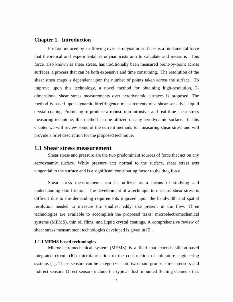
Figure 1.1 Schematic of a typical floating

point. Subscript t indicates tether dimension.

Subscript e indicates element dimension. g is

the height of the gap between the floating

element and the substrate. t is the thickness

of the element and the tether. The figure is

adapted from Naughton and Sheplak [5].

integrate force produced by the wall

shear stresses. Direct sensors using

floating element on a macro-scale

have been extensively developed;

however, due to constraints on

dimensions, it is almost impossible for

macro-scaled floating element sensor

to achieve the dynamic bandwidth and

spatial resolution that are needed to

measure the shear stress in a turbulent

boundary layer. This is because the

dynamic bandwidth of the floating

element is directly proportional to its

natural frequency. A schematic of

typical floating element design is

shown in Fig. 1.1 [5]. The

displacement Δ can be correlated to

shear stress τw through Euler-Bernoulli

beam theory as shown in Eq. (1)

(

) , (1)

where A is the area of the element exposed to the shear stress and E is the elastic

modulus of the tether material. Assume the tether to element area ratio is close to zero,

the spring constant of the tether can be estimated using Eq. (2)

. (2)

The dynamic bandwidth of the floating element can be estimated using the natural

frequency of the device as shown in Eq. (3).

√

√

. (3)

3

Figure 1.2 Schematic of the optical shutter

design. Integrated photodiodes are under

different areas of exposure. This figure is

adapted from Padmanabhan [6].

Simple dimensional analysis using Eq.

(3) can show that by reducing the size

of a 1cm x 1 cm x 1mm floating

element to 100 µm x 100 µm x 1 µm,

the dynamic bandwidth can be

improved at least five-orders of

magnitude [5]. Realizing such benefits,

Schmidt et al. [2], first exploited the

micromachining technology by

developing a polyimide/aluminum

surface, and a differential capacitive

technique to measure the movement of

the floating element. It demonstrated the huge potential of MEMS, including a high

dynamic bandwidth up to 10 kHz, large dynamic range of 0.01-1Pa, etc. However it has

also shown to be problematic. Moisture variations changed the mechanical properties of

the polyimide which led to mechanical sensitivity drift [5]. The technique is also prone

to electromagnetic noise interference (EMI). Other methods, including piezoresistive

based [3, 4], force-feedback capacitive based [7, 8], and optical shutter-based [9, 6, 10,

11], have then emerged to perfect this technology. Among these, the optical shutter-based

sensors stand out as a new potential candidate for MEMS. Figure 1.2 illustrates the

schematic of this design. It has a demonstrated maximum nonlinearity of 1% over a

dynamic range spanning from 1.4mPa to 10Pa. It also possesses a verified bandwidth of

up to 4 kHz, which has been qualitatively shown to exceed 10 kHz [11, 12]. Unlike the

differential capacitive technique, it is also insensitive to environmental effects such as

moisture and EMI. It is, however, sensitive to the position variation of the light source

which is mounted separately. Though the advantages of direct MEMS compared to their

macro scale counterparts are significant, they are not without limitations. Winter [13]

summarizes these limitations as follows:

(1) The spatial resolution is constrained by the dynamic range of the sensor.

(2) Sensor packaging and installation caused errors.

(3) Pressure gradients caused measurement errors.

4

(4) Cross-axis sensitivity due to thermal expansion, vibration, and acceleration.

Indirect MEMS rely on empirical or theoretical correlations to relate the measured

quantity to shear stress. Examples include thermal films [14, 15, 16] and laser Doppler

measurement [17, 18] as well as the recently developed micro-pillars [19, 20]. Thermal

films have recently surpassed the near-wall hot-wire method as they are guaranteed to be

within the boundary layer and they are insensitive to the pitch angle of the flow. Thermal

films operate on the similar principle to the near-wall hot-wire anemometer. As heat

transfers away from the hot-film sensor, the resistance of hot-film changes according to

the temperature variation. Since the variation of the heat transfer rate is mainly due to the

convective heat transfer within the fluid, the signal caused by this resistance variation can

be used to measure the wall shear stress. A widely used general scaling approximation of

the relationship is that the Nusselt number of the sensor is proportional to the wall shear

stress to the third power. This relationship has been used with the assumption that the

thermal boundary layer generated by the hot-film is fully submerged under the boundary

layer. In the review paper written by Haritonidis[21], this scaling relationship was shown

to be valid only when the Peclet number is above 100. As one of the most developed

shear stress measuring techniques, hot-films have shown promising results at various

situations such as during transition, local separation, or shock oscillation [15]. One of the

drawbacks of the hot-film sensors is the difficulty of obtaining a unique relationship

between the heat transfer and the wall shear stress. This is due to the heat transfer being

a function of a multitude of parameters such as substrate heat conduction and yaw angle

of the flow. Haselbach et al. [15] have pointed out a trade-off relationship between the

dynamic bandwidth and the sensitivity of the sensor based on the choice of substrate

material. Higher thermal conductivity and diffusivity of the substrate material leads to an

increase in the dynamic bandwidth of the sensor at the cost of reduced sensitivity of

sensor. Elvery and Bremhost [14] did a detailed analysis of how the yaw angle of the

flow affects the hot-film signal. Though they demonstrated a relationship between the

yaw angle of the flow and the hot-film signal at a given speed, such a relationship would

be only useful if the streamline information is known. Such parameter dependency

results in the hot-film technology being useful only if it is calibrated ahead of time to the

experimental conditions with a reference method and used in situations where the

5

streamline information is already known. Realizing this need for calibration,

Chandrasekaran et al. [16] have developed a calibration technique that uses a known

super-imposed sinusoidal shear stress over an established mean flow to calibrate the

sensor. Acoustic plane wave excitation of a shear stress sensor allows for calibration up

to a dynamic bandwidth of 20 kHz. The main source of error is caused by the temperature

drift in the mean flow. Another noteworthy limitation of the technique is the spatial

resolution of the sensors. In their analysis of in-line hot-film arrays, Haselbach et al. [15]

have also pointed out that the measurement error increases asymptotically with decreased

spacing of the sensors.

MEMS based on Laser Doppler Effect have also been developed recently and

have shown promising results, such as a 99% accuracy up to Rex = 106 [18]. However its

main limitation at this time is the low near-wall seeding density, since only the seeds

within the sub-viscous layer can be used to estimate wall shear stress. This limits the

technology to measuring the unsteady behavior of the flow.

Micropillars are an emerging technology that has shown a huge potential. This

technology optically measures the tip movement of micro-scale pillars that protrude into

the viscous sub-layer of the flow. Große et al. [19, 20] have done extensive work deriving

a correlation between the tip movement of the pillars due to the fluid bending force and

the wall shear stress. In their derivation, a linear velocity profile within the sub-layer of

the fluid is assumed. Based on this correlation, Micropillars can give a detailed shear-

stress measurement of both magnitude and direction over a large area with sufficient

spatial resolution. With current technology, Micropillars can be manufactured from a

height range of 80 to 1000 µm and an aspect ratio of 15-25. This physical limitation sets

the upper limit of the dynamic bandwidth of the sensors, which currently has been only

measured up to 2050 Hz [19]. A 10-15% gain yield bandwidth is predicted due to

improvements of the manufacturing technology. The lowest dynamic range limit is set by

the noise level of measurement, which makes the current smallest detectable wall shear-

stress to be about 10mPa [19]. Micropillars emerge as a promising technology because of

their ability to measure both the magnitude as well as direction with a much better spatial

resolution than other aforementioned MEMS based technologies. It does have a few

6

Figure 1.3 Interference pattern produced by

Fizeau Interferomery. (a) Fringe pattern at

time t = t1. (b) Fringe pattern at t = t2. Light

either constructively or destructively

recombines to form the fringe pattern which

changes according to the shear stress. The

figure is adapted from Naughton and Sheplak

[5].

drawbacks, including a limited

temporal resolution as well as the

intrusive nature of the method. Even

with a predicted 10-15% increase of

dynamic bandwidth, a 2 kHz

dynamic range cannot allow this

technology to be competitive with

other high temporal resolution

technologies such as the optical

shutter based MEMS. Since the

current technology requires the

sensors to be illuminated from

underneath, models being measured

have to be made of a transparent

material; this leads to greater design

and construction complexity. These

disadvantages are likely to be

improved with further work and

development. They have also been developing a reflective illumination technique to

improve the invasive nature of the method. Another disadvantage is due its small size and

the optical measurement nature. In order to be able to see the individual pillar, the field of

view must limited within a 6 cm x 6 cm area. This drawback limits its capability of being

used on a bigger scale, such as wind tunnel applications.

1.1.2 Thin oil film

Squire [22] first derived the thin-oil-film equation to prove that the oil-film

technique that often is used in wind tunnels as a streamline visualization method actually

indicates the streamline pattern. Squire found that oil followed surface streamlines

except when separation happened; he also proved that oil film has little effect on the

boundary layer. Tanner and Blows [23] first realized the potential of this theory to be

utilized as a surface shear stress measurement technique. They simplified Squire’s thin-

oil-film equations to present a simpler correlation between thinning rate to surface shear

7

stress. They also decided to use interferometry as their method to measure the thickness

of the oil film. This became the predominant technique for all oil film shear stress sensors.

The principal of interferometry is illustrated in Fig. 1.3. When the incident light hits the

thin oil film, part of the light reflects off the surface of the film while the rest of it is

reflected from the substrate. The thickness of the film decides the phase delay between

the two reflected light beams. This phase delay causes the reflected lights to either

constructively or destructively combine together. This induces a fringe pattern that can be

seen from the interferometry: the destructive part darkens while the constructive part

lights up. This fringe pattern can be correlated back to the thickness of the film which in

turn can be correlated back to shear stress based on Squire’s thin-oil-film equation.

Another major advancement of the technique occurred a decade later when Monson et al.

[24, 25] at NASA Ames recognized that the thin-oil-film equation can be integrated, thus

only one image by the end of the test would be sufficient to derive the mean shear stress.

They also introduced a few surface techniques that can be used on normal wind tunnel

data that will give a good fringe pattern. This along with Tanner and Kulkarni’s [26]

suggestion of using oil drops instead of a continuous oil-film have pushed thin-oil-film

technology to where it is today. The current thin-oil-film technologies can be categorized

into two groups: 1-D and 2-D. The 1-D technologies are based on the aforementioned

techniques, using oil drops over a large area with only one image being taken after the

test, are sufficient to determine both mean shear stress magnitude as well as direction.

The simplicity of the technique, however, leads not only to a significant advantage but

also to a considerable drawback. The single image by the end of test method basically

neglected any transient behavior of the flow. This results in the technique being useful

only for steady-state shear stress measurement. The 2-D technology is based on a

discretized version of Squire’s thin-oil-firm equation. It links the 2-D shear stress to the

location and height of the oil-film. Unlike the 1-D method, this technique requires two

images to be taken in order to calculate the mean shear stress in between the two

instances. Since shear stress is only averaged between the two frames, temporal

resolution is dramatically improved. The spatial resolution of the method, however,

remains fairly low, since oil drops have to be separated by their streak distances. Thin oil

films are also sensitive to environmental conditions such as temperature of the flow

8

Figure 1.4 Sub-states of liquid crystal. [5]

which affects the viscosity of the oil. Dust and humidity of the flow can also destroy the

fringe pattern.

1.1.3 Liquid crystal

Liquid crystal is a state of

matter that is between solid and liquid.

It behaves like liquid on macroscopic

scale; however, it shows order in

molecular arrangement on a

microscopic scale. Normally liquid

crystal molecules have a long rod

shape, which gives them two unique

refractive indices, one measured along

the long axis of the rod and one

measured perpendicular to it. The

direction where the long axis points to

is called director. Figure 1.4 shows some of the normal molecular arrangements that most

liquid crystals can take at different temperatures. Due to the unique property of dynamic

birefringence, liquid crystals are ideally suited to be utilized as a means of measuring

shear stress. There are two major techniques in shear-sensitive liquid crystal: color based

and intensity based. Chiral nematic liquid crystals are normally chosen in color based

technique. In this state, liquid crystals form a helix structure where all liquid crystals in

each layer share a common director that is parallel to the layer. These directors twist at

different angles across different layers to form the helix pattern. If the vertical axis of the

helix structure is parallel to the normal of the substrate then it is called the Grandjean

state; otherwise it is called Focal Conic state. A change in selective reflection in light can

happen either when liquid crystal changes from Focal Conic state to Grandjean state or

when the pitch of the helix pattern changes. Both of these motions can be induced by

shear stress. The change in selective reflection results in a change of color that is also

dependent on viewing angle. Reda, et al. [27, 28, 29] at NASA Ames research center

capitalized on this concept and demonstrated a shear stress measurement technique based

on the color observation of the sample. Since color is a function of viewing angle,

9

multiple images at different viewing angles have to be used in order to establish a

Gaussian distribution and find the true hue of the color. This limitation not only places a

stringent requirement on the mounting angle of the cameras but also makes

measurements on any curvilinear surface difficult to calibrate. Recently, however,

Fujisawa et al. [30] demonstrated that by using only two cameras, they can acquire the

shear stress measurement over a NACA 0018 airfoil. Another disadvantage of this

technique is the complex data analysis. The biggest advantage of the liquid crystal

technique is near infinite spatial resolution. Reda, et al. [32] also studied the temporal

resolution of the liquid crystal, which they concluded to be on the order of 1 kHz. Unlike

color based technique, intensity based technique normally uses nematic liquid crystal. In

this state, order only presents in a common director in liquid crystal direction. No

positional order exists in this state. This means it is more flexible then the chiral nematic

state. Shorter response time, therefore, can be expected comparing to the chiral nematic

state. When subjected to shear stress, the director of the liquid crystals aligns according to

the magnitude and direction of the shear stress. This motion causes a corresponding

change of birefringence value of liquid crystals. This change in birefringence value can

be simply detected by placing the sample in between a pair of crossed linear polarizers.

When the birefringence value is low, the crossed linear polarizers let a very small amount

of light through. The intensity of the light passing through this sandwiched set starts

increasing as the birefringence value increases. Buttsworth et al. [31] did a full-field-

shear-stress-measurement based on this theory. However, a major disadvantage of both of

these techniques is the temporal resolution. Even though the liquid crystal has a relatively

small response time, the motion of the liquid crystal is irreversible. Theoretically, the

resolution can be improved by comparing frame-to-frame changes of the sensor.

However, since both techniques can only be calibrated under a steady flow, it is almost

impossible at this stage to resolve the frame-to-frame change of shear stress.

1.2 Shear-Sensitive Polymer Dispersed Liquid Crystal Shear-sensitive polymer dispersed liquid crystal (PDLC) was developed to

overcome the aforementioned disadvantages of shear-sensitive liquid crystal techniques.

First introduced by Parmar and Singh [33], shear-sensitive PDLC utilizes the structure

rigidity provided by the polymer film to improve the temporal resolution of the sensor.

10

However, he didn’t relate the signal

to shear stress, nor did he study the

reversibility of the PDLC. When

the proper polymer is mixed with

liquid crystals, liquid crystals form

droplets within the polymer film.

Nematic liquid crystal was

normally chosen to make the PDLC

sensor. As the second most

disordered liquid crystal state next to the isotropic state, nematic liquid crystal, therefore,

inherently has a low viscosity and a fast response time. All liquid crystals within one

droplet share a common director. If there was no external aligning field when the film

was cured, these directors across different droplets will point at random directions. As

shown in Fig. 1.5 when subjected to a shear stress, these liquid crystal droplets elongate

according to the shear stress. This motion causes the directors to align. The alignment of

the nematic liquid crystal gives a coherent change in PDLC’s birefringent value, which

can be correlated back to the shear stress. If the polymer was chosen in such a way that

the refractive index of the polymer matches the one of the refractive index of the liquid

crystal, the birefringent value change from each droplet in the PDLC sensor is similar to

that of the intensity based shear stress sensor. However, adding polymer into the film is

not without complications. If the droplets’ size is around one order of magnitude bigger

than the visible light, the randomly initial alignment of the droplets induces a strong

scattering effect. Since the birefringent value can only be optically determined, light

transmission is critical for the birefringence measurement. This scattering effect can be

improved through an initial alignment of the droplets’ directors. Though it has not been

tested within this study, the theoretical benefits of the initial alignment will be elaborated

later in this paper. Another complication is the added temporal resolution dependency on

the PDLC film’s response time. The response time of the liquid crystal is no longer the

sole determinant factor of the temporal resolution of the sensor. Instead it is dependent on

the smallest response time between the liquid crystal and the PDLC film. The response

time of the PDLC film can be estimated using the shear wave velocity of the PDLC film

Figure 1.5 PDLC under shear stress. Yellow

arrows represent the directors of liquid crystals

inside a droplet. The black lines inside circles

represent the liquid crystal molecules. These

directors align according to the shear stress.

11

and the thickness of the film. The shear velocity defined in Eq. (4) describes how fast

shear waves travels in the elastic material.

√

, (4)

where G and are the shear modulus and the density of the material respectively. The

response time of the PDLC film can then be estimated using the thickness of the film

divided the shear velocity. Since the normal thickness of the PDLC film is on the order of

10 µm, this estimation shows that the PDLC film’s response time is at least two orders of

magnitude smaller than that of the response time of the liquid crystal. Therefore the

temporal resolution of the PDLC sensor is determined by the liquid crystal’s response

time.

1.3 Imaging polarimetry system As mentioned before, color based liquid crystals have to face the challenge of

complex data analysis. Though

intensity based liquid crystal’s

signal can be measured simply

using a pair of crossed linear

polarizers, this method doesn’t take

the full advantage of liquid crystal

sensor, this because it can’t obtain

directional information. In an effort

to improve upon this method, a

better acquisition system that is

easy to use and can provide

detailed birefringent value and direction is in need. Glazer, Lewis and Kaminsky [34]

first laid the foundation for the possibility of such a system. They presented a method

utilizing circular polarized light as the light source. When circular polarized light passes

through a birefringent media, each of the two refractive indices gives different phase

retardations to the light. This phenomenon changes circular polarized light into

elliptically polarized light, with the long and short axis proportional to the two distinct

Figure 1.6 Elliptically polarized light. ϕ is the

extinction angle measured from the slow axis

(larger refractive index) to the horizontal (with

respect to the linear polarizer.)

12

refractive indices. Thus, the birefringence can be determined by measuring the properties

of the elliptically polarized light. This elliptically polarized light also contains directional

information. Birefringent material inherently contains an extinction angle. If the material

placed at the extinction angle no light would be able to pass through, since the two

reflected lights lines up with the angles of the two crossed linear polarizers. This

phenomenon occurs four times every rotation placed π/2 apart. In elliptically polarized

light, this extinction angle is shown in Fig. 1.6. It can be used to relate back to the

direction of the shear stress, since this extinction angle describes the direction the ellipse

is pointing to. Glazer, Lewis and Kaminsky [34] in their paper demonstrated a system

using a rotating linear polarizer to detect the elliptically polarized light passed from the

birefringent media sample. The key concept behind this technique is listed in Eq. (5) [34].

[ ]. (5)

I0 is the initial intensity of the circular polarized light and I is the intensity measured

behind the rotating linear polarizer. The frequency of the rotating polarizer is ω and t is

time. The phase shift δ is a value that can be used to correlate to the birefringence as

shown in Eq. (6) [34].

. (6)

λ is the wavelength of the light. is the birefringence value and L is the thickness of the

birefringent material. In the PDLC film the birefringence is only a function of the angle

between the director of the droplet and the substrate normal as shown in Eq. (7) [36], if

the polymer’s refractive index is close to the refractive index of the liquid crystal

measured along the long axis.

, (7)

where ne and no are the extraordinary and the ordinary refractive indices of the liquid

crystal respectively. The angle between the liquid crystal director and the substrate

normal is θ.

As can be seen by measuring the intensity of the elliptically polarized light

passing through the rotating linear polarizer, both the birefringence and the direction can

13

be calculated. Kaminsky et al. [35] later improved this method by realizing that only four

intensity values are enough to determine the birefringence and the extinction angle, if

they can be taken simultaneously behind four differently aligned linear polarizers. This

can be seen through changing the time dependent term in Eq. (5) with a set of angles

αi at which the linear polarizers are placed at as shown in Eq. (8) [35].

[ ]. (8)

Since are the only variables, Eq. (7) can be linearized and expressed in form of

Eq. (9) [35].

, (9)

where a0, a1, and a2 are coefficients that can be linked back to , ϕ, and δ through the set

of equations shown in Eq. (10) [35].

,

,

. (10)

They also can be calculated using the intensity values measured as shown in Eq. (11) [35].

∑

, ∑

, ∑

. (11)

If these linear polarizers are set at angles 0o, 45

o, 90

o and 135

o, Eq. (11) can be taken in

forms of Eq. (12) [35].

∑

, ∑

,

. (12)

The term which is a function of the birefringence only and can be calculated

using Eq. (13) [35].

√

. (13)

The extinction angle, which contains the shear stress directional information, can

be expressed as in Eq. (14) [35].

14

(

√

). (14)

Based on this algorithm, Kaminsky et al. [35]

then developed a real time birefringence and

extinction angle measurement system called

“MilliView”. It utilizes an image-multiplexing

device that has been developed by Optical Insights,

LLC (Santa Fe, NM) that makes real-time

birefringence and extinction measurements a reality.

The device, known as Quad-View, is essentially a

camera lens fitted with a 4-sided prism. This prism

splits the sample image into four reflections that are

mirrored back to a CCD camera. The resulting four

simultaneous images are then focused on the surface

of the camera as an array. The Quad- View is fitted

with four linear polarizers set at the aforementioned

angles thus eliminating the need for mechanical

rotation. Figure 1.8 demonstrates the functional

groups of the Quad-View system. This system, “MilliView”, revolutionized intensity

Figure 1.8 Optical components of

“MilliView”. 1. Light source; 2.

Bandpass filter; 3. Circular

polarizer; 4. Sample; 5. Quad View;

6. Color CCD camera.

Figure 1.7 Functional Groups of Quad-View. Light from the sample enters the prism

and splits into four beams bouncing back from the mirrors before it goes through four

differently aligned linear polarizers. Then the four intensity images go in to the CCD

chip. Note: The linear polarizers must be adjusted such that the mirror effects are

accounted for.

15

based shear sensitive liquid crystal by producing real-time images that generate

quantitative maps of sin (δ) and θ. The optical components of “MilliView” are shown in

Fig. 1.7.

1.4 Objectives The objectives of the current project comprise of the following points listed below.

1.4.1 Wind tunnel applicable

As most of the current shear-sensitive liquid crystal applications stay in the

experimental stage, the object of this project is to push this technology one step closer to

being utilized in a commercial set up. In order to achieve this object, a series of obstacles

must be overcome. The light source and imaging system should stay outside the wind

tunnel and must not move with respect to each other and to the tested model. This means

the system must be able to overcome the vibrations of the wind tunnel and still capable of

accurately measuring shear stress. It also must be insensitive to other parameters such as

temperature, humidity, expansion of the window when the wind tunnel is running, and

fine particulate matters.

1.4.2 Uniform and high signal-to-noise ratio

The PDLC sensor must not change the nature of the flow over the tested surface.

This requires the PDLC film to be smooth. It also needs to be able to provide uniform

results across the entire testing surface. Thus, the sensor will not need to be calibrated

locally. In order to provide useful results, it also must have a sufficient signal-to-noise

ratio. Only proper polymer and liquid crystal combinations can form good PDLC film.

However, this process is complicated and depends on various variables. This means only

through testing different combinations, the performance of the PDLC can be concluded.

There is no existing theory to predict which combination would work well. Various

application methods need to be tested as well, such as airbrushing, direct deposit, and

spin coating.

1.4.3 Macro scale imaging with high resolution

In order to become feasible in wind tunnel application, the optical system needs to

be able to provide a detailed 2-D shear stress map over a large testing surface. This puts

16

stringent requirements on the optical system. The light source must be strong enough to

provide sufficient and uniform lighting across the testing surface. The imaging system

must be able to zoom in a relatively large area with enough resolution to provide detailed

information. Since the aforementioned Quad-view system spilts the incoming image into

four identical images, each of these four images can only obtain at maximum one quarter

of the intensity of the original image. The CCD chip’s field of view is also reduced to one

quarter of the original area at maximum. This puts even higher restrictions on the light

source and the optical system.

17

Chapter 2. Experimental facilities, instrumentation and set up

2.1 Calibration facilities

Figure 2.1 illustrates the schematic of the experimental apparatus. The key

component is a Jet Stream 500 wind tunnel. Using the measured wind speed from a Pitot

tube inside the test chamber as feedback signal, Jet Stream 500 utilizes a proportional-

integral-derivative (PID) controller to adjust the input power to the 1 hp AC motor

providing user designated wind speed from 0 to 80 MPH. To avoid birefringence effect,

all the transparent sides of the test chamber were sealed using annealed thick glass. The

cross section of the test chamber is 5.25 inches by 5.25 inches square. The Pitot tube was

adjusted to the side of the chamber to avoid the sample affected by the flow disturbance

induced by the Pitot tube. A precision rotational stage was constructed to position the test

plate inside the test chamber such that the tested aerodynamic surface can be set to an

angle of attack ranging from -17o to + 17

o in one degree steps. Detailed drawings of the

test chamber can be found in Appendix A.

Light is provided by a Lumitex, Inc 2-Port Source powered by a 21V, 150W

halogen lamp. The 150W halogen lamp provides more than sufficient lighting required

for the back lighting scheme where the sample is in between the light source and the

imaging system. Light coming from the light source first encounters a diffuser plate to

Figure 2.1 Experimental Apparatus. Light from the light source passing through the

diffuser and the circular polarizer becomes circular polarized. Then it passes though the

sample enters the Quad-View system before it is captured by the CCD camera. CCD

camera sends the collected image to be analyzed in the Milliview.

18

make the illumination more uniform across the testing area. A circular polarizer set is

placed immediately after the diffuser. It consists of a linear polarizer and a quarter wave

plate laminated together at an angle that is optimized for 570nm wavelength. The diffuser

plate and the circular polarizer set is laminated together and placed on the side of the

wind tunnel test chamber.

Current PDLC films are tested on 25 mm x 75 mm glass micro-slide substrate that

is placed in the middle of the test chamber. On the other side of the wind tunnel, the

imaging system consists of an adjustable lens, the Quad-View system, and a CCD camera

that are secured together on the same frame structure which is also supporting the light

source. This frame structure is also clamped on the test chamber using 6 C-Clamps. This

set up makes sure that the light source, test sample, and the imaging system will have

minimum movement relative to each other, despite the vibration caused by the running

wind tunnel. The lens used in the imaging system is a Computar 1/2” 4-8mm Megapixel

Lens with manual iris. The specification sheet of the lens is provided in Appendix B. The

CCD camera used in this set up is a 3.0 mega pixel Am Scope MD 800 E color CCD

camera. The “MilliView” software is installed on a computer that is connected to the

CCD camera using a USB 2.0 cable.

Figure 2.2 Calibration facilities. Omitted details can be found in Fig. 2.3.

19

Figure 2.2 and 2.3 are images of the testing facilities with detailed description of

each component.

2.2 Calibration set up and technique The calibration tests are conducted in the following way. The sample was first

secured inside the test chamber and then tested at a series of speed points. Typical tests

consist of speed points at 13, 26, 39, 52, 65 and 80 MPH. In each test, after the sample

was secured, an initial birefringence map was taken and set as the background of

the map. Any new map collected after this point, therefor would be the

result of the real map subtracting this original map. As previously

mentioned, the non-aligned PDLC films have liquid crystal directors pointing at random

directions. By subtracting the initial map, only the change in would show

up as signal, this improves the signal coherency. After this process is finished the data

were collected while the wind tunnel was running at the first speed point. Then the wind

tunnel shuts down and another set of data was collected to compare with the initial

background to see if any changes occurred. This method tests the repeatability of the

PDLC film. Unless otherwise noticed in the description of the test, this process repeats

five times before moving on to the next speed point. The overall the experimental inquiry

is complete after all five speed points are tested.

Figure 2.3 Calibration facilities: testing chamber.

20

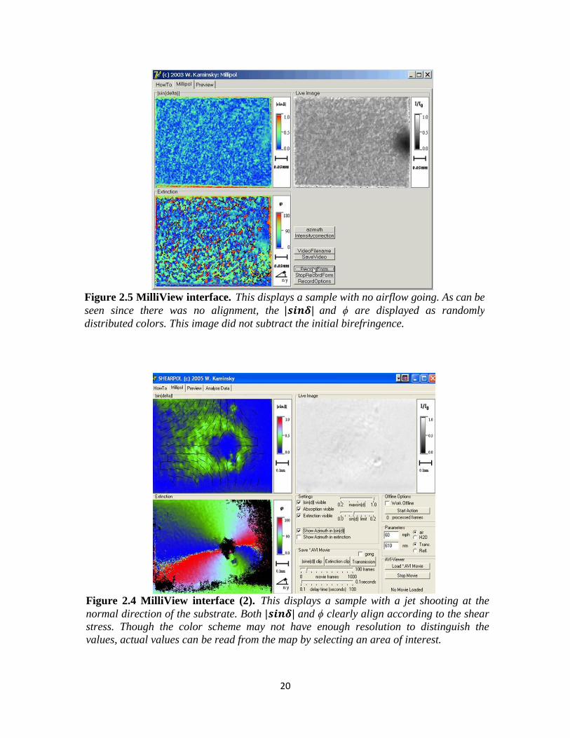
Figure 2.4 MilliView interface (2). This displays a sample with a jet shooting at the

normal direction of the substrate. Both 𝒔𝒊𝒏𝜹 and ϕ clearly align according to the shear

stress. Though the color scheme may not have enough resolution to distinguish the

values, actual values can be read from the map by selecting an area of interest.

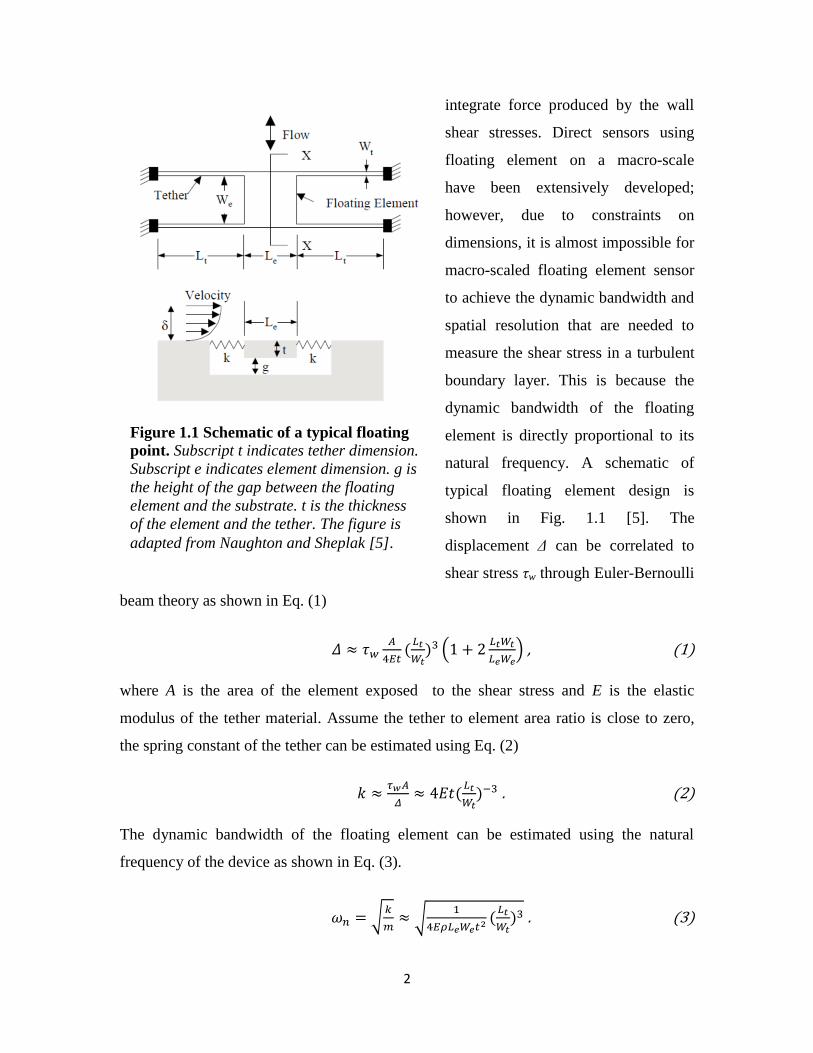
Figure 2.5 MilliView interface. This displays a sample with no airflow going. As can be

seen since there was no alignment, the 𝒔𝒊𝒏𝜹 and ϕ are displayed as randomly

distributed colors. This image did not subtract the initial birefringence.

21

2.3 Data analysis

Data was collected in the “MilliView” system. It displays the map using a

color bar scheme. The value increases from 0 to 1as the wavelength of the color

increase from blue to red. The extinction angle ϕ is displayed in a similar fashion. It

increases from 0o to 180

o as the wavelength of the color increases from blue to red. The

“MilliView” interface is illustrated in Fig. 2.4 and Fig. 2.5. Since and ϕ are

displayed at per pixel resolution, data can acquired at same resolution level. Normally an

area of interest is selected, instead of analyzing the whole map. “MilliView” displays the

average value of the over the selected area, which was then recorded and plotted

for results. Since the tests performed were unidirectional, the extinction angle was not

recorded.

The shear stress at each of the speed points was estimated using 1/7 power law

derived by Theodore von Kármán as shown in Eq. (15), since the thickness of the micro-

slide would trip the flow into turbulence boundary layer even at 13 MPH.

, (15)

where Cf is the skin friction coefficient defined in Eq. (16) and Rex is the Reynolds

number based of distance measured from leading edge as defined in Eq. (17).

, (16)

where is the wall shear stress, ρ is the air density here, and U∞ is the free stream

velocity.

, (17)

where x is the distance measured from leading edge and µ is the dynamic viscosity of the

air here. A plot of the shear stress at 13 MPH is given in Fig. 2.6.

The shear stress correlates to a shear strain according to Eq. 18 as shown

below.[37]

22

. (18)

The change of the director angle Δθ for an initially aligned PDLC film relates to the shear

strain by Eq. 19 as listed below.

Δθ

. (19)

The signal measured by “MilliView” can be related to shear stress using Eq.

6,7,18, 19, as expressed below.

[

(

) ] . (20)

The shear stress can be then related back to velocity using Eq. 15 and 16 as shown below.

. (21)

Figure 2.6 Shear stress versus distance at 13 MPH. The shear stress is plotted over the

micro-slide estimated using the 1/7 power law versus distance from leading edge.

23

At the same location, neglecting the change in the thickness of the film, the signal

relates to free stream velocity U by Eq. 22,

[

] , (22)

where C1 and C2 are defined in the following equations respectively.

, (23)

. (24)

For films around 15µm thick, C1 is on the order of 102. However the shear-modulus of

the PDLC films is hard to determine, since the structure of PDLC makes it a composite

material with liquid-crystal-solid properties. A value of C2 on the order of 10-4

is

chosen as shown in Fig. 2.7 to demonstrate how the velocity, signal relationship would

look like without any particular meaning. This relationship is confirmed in “Results”

section through a number of plots.

Figure 2.7 Signal Velocity Profile. A plot of signal versus velocity profile with C1 equals

to102 and C2 equals to 10

-4.

24

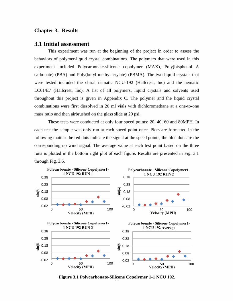
Figure 3.1 Polycarbonate-Silicone Copolymer 1-1 NCU 192.

Chapter 3. Results

3.1 Initial assessment This experiment was run at the beginning of the project in order to assess the

behaviors of polymer-liquid crystal combinations. The polymers that were used in this

experiment included Polycarbonate-silicone copolymer (MAX), Poly(bisphenol A

carbonate) (PBA) and Poly(butyl methylacrylate) (PBMA). The two liquid crystals that

were tested included the chiral nematic NCU-192 (Hallcrest, Inc) and the nematic

LC61/E7 (Hallcrest, Inc). A list of all polymers, liquid crystals and solvents used

throughout this project is given in Appendix C. The polymer and the liquid crystal

combinations were first dissolved in 20 ml vials with dichloromethane at a one-to-one

mass ratio and then airbrushed on the glass slide at 20 psi.

These tests were conducted at only four speed points: 20, 40, 60 and 80MPH. In

each test the sample was only run at each speed point once. Plots are formatted in the

following matter: the red dots indicate the signal at the speed points, the blue dots are the

corresponding no wind signal. The average value at each test point based on the three

runs is plotted in the bottom right plot of each figure. Results are presented in Fig. 3.1

through Fig. 3.6.

25

Figure 3.2 Polycarbonate-Silicone Copolymer 1-1 E7.

Figure 3.3 PBA 1-1 E7.

26

Figure 3.4 PBMA 1-1 NCU 192.

Figure 3.5 PBA 1-1 NCU 192.

27

Figure 3.6 PBMA 1-1 E7.

As can been seen in this study, PBA was the most flexible polymer among the

three polymers that were tested, since it gave the best signal-to-noise ratio. The E-7 liquid

crystal generally had a higher signal strength compared to NCU 192. This initial

assessment demonstrated the feasibility and the potential of this project. The PBA and E-

7 combination particularly showed a good signal-to-noise ratio and high reversibility.

This study also helped us to discover some problems that the system had at the time, such

as the reversibility change between the first run and later run. This problem was

concluded to have been caused by the vibration movement when the wind tunnel was

running. It was later fixed by adding additional C-Clamps to improve the rigidity of the

supporting structures.

3.2 Air brushing study A series of tests were done with all the test samples airbrushed onto the substrates.

Airbrushing is one of the few ways that can be tested in a controlled manner. It gives a

rather uniform surface finish as compared to other methods. The thickness of the film can

be controlled by changing the amount of the solution to be airbrushed onto the substrate.

28

Figure 3.7 PBA NCU-192 Non-revived

In this study, the polymer alone was first airbrushed onto the substrate. Then the

liquid crystal was sprayed on top of the polymer in two different fashions: revived and

non-revived initialed R and N respectively in the figures. In revived fashion, after a

specified time from when the polymer was airbrushed, pure solvent was airbrushed onto

the polymer substrate. The liquid crystal dissolved in solvent was then airbrushed onto

the substrate. In the non-revived fashion, liquid crystal dissolved in the solvent was

directly airbrushed onto the polymer substrate at the specified time. The number in the

figure title after the initial N or R indicates how many minutes after when the polymer

was airbrushed was the solvent or the liquid crystal-solvent mixture airbrushed.

Poly(bisphenol A carbonate) (PBA) and Dimethylsiloxane-bisphenol A-polycarbonate

block co-polymer (MAX) were the two polymers used in this experiment. The liquid

crystal that was used in this experiment is LCR-NCU192. Dichloromethane was used as

the common solvent. The tests were done in a typical fashion of having six speed points

at 13, 26, 39, 52, 65 and 80MPH and repeating five times at each point. Unless otherwise

noted all tests were done in this fashion. The results are shown in Fig. 3.7 to Fig. 3.10.

29

Figure 3.9 MAX NCU-192 Non-revived

Figure 3.8 PBA NCU-192 Revived

30

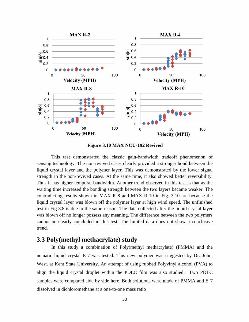
Figure 3.10 MAX NCU-192 Revived

This test demonstrated the classic gain-bandwidth tradeoff phenomenon of

sensing technology. The non-revived cases clearly provided a stronger bond between the

liquid crystal layer and the polymer layer. This was demonstrated by the lower signal

strength in the non-revived cases. At the same time, it also showed better reversibility.

Thus it has higher temporal bandwidth. Another trend observed in this test is that as the

waiting time increased the bonding strength between the two layers became weaker. The

contradicting results shown in MAX R-8 and MAX R-10 in Fig. 3.10 are because the

liquid crystal layer was blown off the polymer layer at high wind speed. The unfinished

test in Fig 3.8 is due to the same reason. The data collected after the liquid crystal layer

was blown off no longer possess any meaning. The difference between the two polymers

cannot be clearly concluded in this test. The limited data does not show a conclusive

trend.

3.3 Poly(methyl methacrylate) study In this study a combination of Poly(methyl methacrylate) (PMMA) and the

nematic liquid crystal E-7 was tested. This new polymer was suggested by Dr. John,

West. at Kent State University. An attempt of using rubbed Polyvinyl alcohol (PVA) to

align the liquid crystal droplet within the PDLC film was also studied. Two PDLC

samples were compared side by side here. Both solutions were made of PMMA and E-7

dissolved in dichloromethane at a one-to-one mass ratio

31

by weight. The PVA was dissolved in hot water and then deposited on top of one of the

micro-slides. The PVA film was a clear and uniform film after it was completely cured. It

was then mechanically rubbed with a velvet cloth in a unidirectional fashion. This is a

well-known technique to align nematic liquid crystals. The theory is that the

microgrooves formed on top of the polymer film due to this mechanical rubbing will

align the liquid crystal directors along the direction of the grooves. Based on this theory,

the assumption in this study was that the liquid crystal droplets would behave similarly to

liquid crystal in these microgrooves. After the rubbed PVA substrate was prepared, the

solution of PMMA and E-7 combination was directly deposited on top of this substrate as

well as a regular glass substrate. The results of this test are shown in Fig. 3.11.

Both of the samples presented better characteristics including high signal-to-noise

ratio and high reversibility over the previously studied samples. However the attempt of

using a rubbed PVA substrate to align the PDLC film failed. Both films presented strong

scattering effects and a rough surface. They both formed goose-bump like structures on

the surface; each bump had very strong scattering effect. This suggested the liquid

crystal directors were not aligned across different droplets. This hypothesis was

confirmed when the birefringence of the samples were visualized in the “MilliView”

software. The inconsistent result at 65MPH was theorized to be due to how the sensor

responds with respect to time. It has been observed that at this wind speed, the sensor had

a fast initial response to the shear stress, however, with relatively lower signal strength.

As the shear stress was sustained, the signal increased gradually. After this there was a

sudden jump in signal strength. Then the signal remained at that value. Thus signal level

Figure 3.11 PMMA 1-1 E7.

32

would vary according to what time relative to the experiment the data was collected. This

phenomenon also presented at 80MPH, however the sudden jump happened almost

immediately as the wind tunnel turned on. Thus, the results at 80MPH show more

consistency. The gradual increase was theorized as being part of the strain stress

relationship of the PDLC films. The sudden jump was theorized as being due to the

sample slightly tipped over at high wind speed, due to a failure of structure support. This

was improved by adding more structure supports.

3.4 Application methods study with PMMA Continuing the successful results found with the PMMA and E-7 combination, a

series of samples using the same combination were tested in this study. However this test

was focused on the application methods such as airbrushing, direct depositing and spin-

coating. In the airbrushing method, toluene was added to the solution to control the

curing rate. With pure dichloromethane the solution tends to cure before it even reaches

the substrate. This resulted in the films to have an undesirable surface finish. The added

toluene helped the solution to cure at a slower rate. In spin coating, the solution was first

poured on top of a glass micro-slide. It was then put in a Clay Adams Readacrit

Centrifuge. A TDGC - 3KM metered variable autotransformer was connected to the

centrifuge to control the spin rate. An airbrushed PMMA and NCU 192 sample was also

tested in this study. Results are presented in Fig. 3.12.

The spin coated sample gave a clear film with a smooth and uniform surface. The

clearness in the film indicated the droplet size of the liquid crystal was smaller than the

wavelength of the visible light. The only other explanation would be that the spinning

motion aligned the directors of liquid crystal droplets. This was highly unlikely to happen

and was confirmed by the birefringence-map taken by the “MilliView”. The spin coated

sample, therefore, had almost no signal over the majority of the film are with the

exception happened on the edge of the film. Data was taken over a small area on the edge

of the film. In the airbrushed sample, the sample presented a smooth and uniform surface

with an opaque film. This is similar in both of the airbrushed samples. The NCU 192

combination showed a colorful opaque film compared to the white opaque film of the E7

combination. The difference is due to the nature of the chiral nematic liquid crystal.

33

The directly deposited sample used a heated solution of PMMA and E7. This gave

the sample a more uniform and smooth surface compared to the previous study. It also

retained its strong scattering effect. The overall results of this study are unsatisfying

compared to the previously study of the PMMA and E7 combination. This study showed

the importance of the application methods. Both the thickness of the film and the curing

rate of the film significantly affected the performance of the sensor.

3.5 Direct deposition study In the previous two studies, the directly deposit method showed more promising

results. Despite its disadvantages such as a non-uniform surface and thickness, it was

used again in this study. A new polymer, polystyrene was introduced in this study. This is

the polymer used by Parmer [33] et al. in their study of PDLC film. Polycarbonate and

PMMA were also used in this study. Both the NCU 192 and E7 were tested with all

polymers. Results are presented in Fig. 3.13.

Figure 3.12 Application methods study.

34

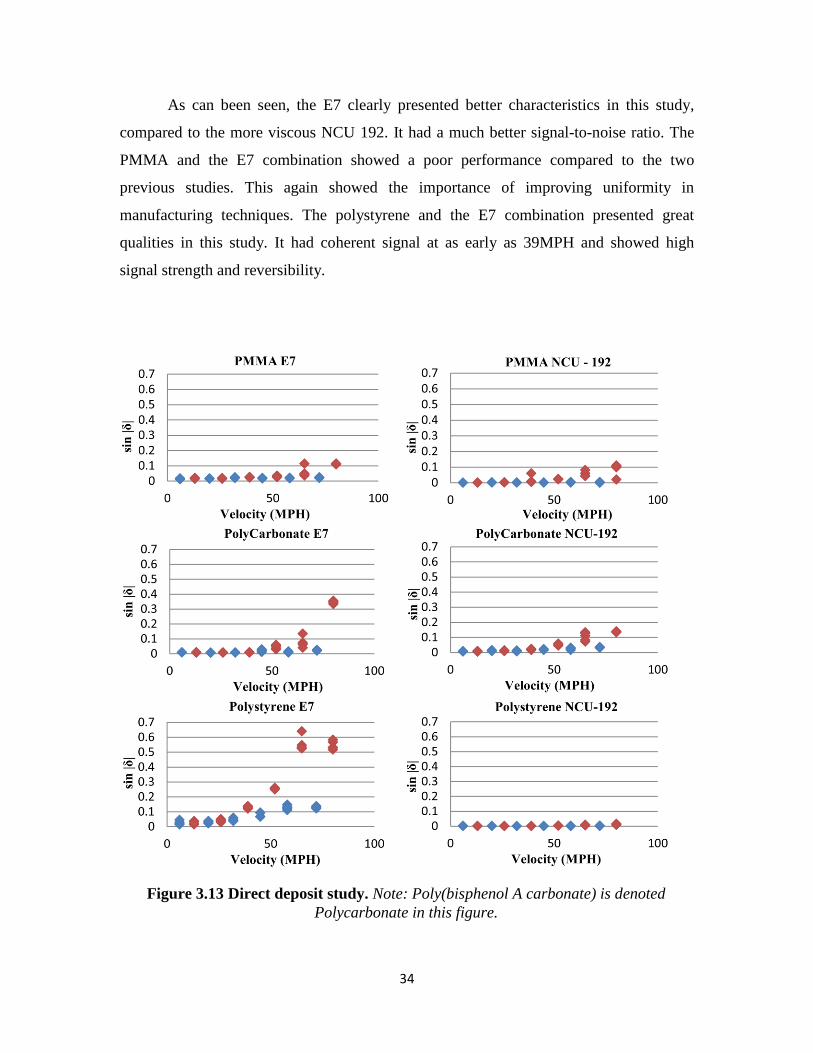
As can been seen, the E7 clearly presented better characteristics in this study,

compared to the more viscous NCU 192. It had a much better signal-to-noise ratio. The

PMMA and the E7 combination showed a poor performance compared to the two

previous studies. This again showed the importance of improving uniformity in

manufacturing techniques. The polystyrene and the E7 combination presented great

qualities in this study. It had coherent signal at as early as 39MPH and showed high

signal strength and reversibility.

Figure 3.13 Direct deposit study. Note: Poly(bisphenol A carbonate) is denoted

Polycarbonate in this figure.

35

3.6 E7 study As was learned from the previous study, the E7 liquid crystal clearly presented a

better signal-to-noise ratio. Thus, in this study only E7 was tested with various polymers

using a direct deposition method. Two new polymers were introduced here: Fluorinated

Acrylic (FIB) and Polysilicone. Compared to other polymers, FIB needs a special solvent,

trifluorotoluene to dissolve. The Polysilicone used in this test on the other hand would

only cure after hardener was mixed in. Two Polysilicone E7 samples were made. In

sample A, the liquid crystal was directly mixed with Polysilicone and hardener, before

being deposited on top of the glass micro-slide substrate. In sample B, the mixture of E7,

Polysilicone and hardener was dissolved in toluene, before being applied on the substrate.

Results are given in Fig. 3.14.

The Dimethylsiloxane-bisphenol A-polycarbonate block co-polymer (MAX) and

E7 combination showed the best results obtained thus far. Though the signal strength is

not as high as a few other combinations such as FIB and E7 as well as PMMA and E7, it

showed a coherent signal at as early as 13MPH. It also had a linear response to the

velocity, is highly consistent over each test points, and is highly reversible. The FIB and

E7 combination showed similar desirable characteristics.

Figure 3.14 E7 Study.

36

3.7 Reproducibility test In this test the reproducibility of the sensor was studied. The previously used

MAX and E7 combination sample was tested in this study after two weeks of room

storage. This test was done in a different manner. The results are shown in Figure 3.15. It

was plotted in the following fashion, from left to right, the sample was tested at 0, 13, 0,

26, 0, 39, 0, 52, 0, 65, 0, 80, 0, 65, 0, 52, 0, 39, 0, 26, 0, 13, 0MPH. Each speed point was

only tested once. The blue dots are at 0MPH and the red dots are at the speed points. The

overall result of this study was satisfying. Except of the results at 65MPH, it was highly

consistent and highly reversible.

Figure 3.15 Reproducibility test.

37

Chapter 4. Future works

For PDLC to become a practical solution to provide 2-D shear stress map, there

remains a significant amount of works needed to be done on this project.

4.1 Uniformity improvement The uniformity of the PDLC samples must be improved. Fabrication techniques

must be improved in such a way that the film can be reproduced using the same technique.

Details such as surface smoothness, droplet size, and film thickness, especially the latter

two cases, need to be controlled through proper fabrication techniques. This would

provide the capability of analyzing how these details affect the performance of the PDLC

films thoroughly.

4.2 Response time study As in all sensing technologies, the temporal resolution of the sensor determines

the capability of it. Therefore it is very important to characterize the temporal resolution

of the PDLC films. The Am Scope MD 800 E color CCD camera can only record videos

at 30 fps. Thus the temporal bandwidth of the PDLC films can only be studied at this

resolution at the best. Equipment has higher temporal resolution is required to determine

the temporal characters of the PDLC films properly. A simple set up with a photodiode

and high speed data acquisition (DAQ) card can achieve this goal.

4.3 Liquid crystal alignment As previously mentioned, the randomly aligned liquid crystal droplets cause a

strong scattering effect in the PDLC film. This limits the thickness of the PDLC film that

can be used. If the films are too thick this scattering effect would not be able to provide

enough light passing through the film for the birefringence to be studied. Another

importance of this technique is that the aligned liquid crystal droplets would theoretically

improve the signal-to-noise ratio of the PDLC film. The alignment would allow all the

droplets inside the PDLC film to respond to the shear stress uniformly, therefore,

improve the signal coherency. These improvements are especially important if a

reflective method to be developed. One of the feasible alignment techniques at current is

38

to impose an electric field while the PDLC is curing. The liquid crystals used in PDLC,

therefore, must be ferroelectric for this to happen. The nematic liquid crystal E-7 that was

used in this study is an example of a ferroelectric liquid crystal.

4.4 Reflective method The development of a reflective method is a key step for the PDLC sensors to

become practical. The current backlight technique would require the substrate to be

transparent. This sets a stringent limit to what kind of surface the sensors can be tested on.

Since the majority of the wind tunnel models are not transparent, a reflective lighting

method becomes the clear solution to this problem. The aforementioned light scattering

effect imposes a challenge on this development. In a reflective lighting method, light

needs to pass through the film at least twice to be detected. This increases the scattering

effect dramatically. Thus, liquid crystal alignment is critical to this development.

4.5 Curved surface measurement Measuring on curved surfaces presents challenges such as curvature-induced

birefringence, making calibration difficult. Without a proper aligning technique, the

curvature of the substrate can induce a strong birefringence. Though initial birefringence

subtraction can help this problem, it also limits the “MilliView” capability such as

direction detection. Another problem arises when using the reflective lighting method,

the elliptically polarized light reflecting off the curved substrate may induce changes in

the extinction angle. This poses great challenges for calibration, perhaps even limiting the

technique to in-situ calibrations on different surfaces.

4.6 Calibration against analytical solution The current shear stress model used in this study is based on the 1/7 power law.

This is an empirical model that is based on a lot of assumptions. Calibration against an

analytical solution would gain a better understanding of how the PDLC behaves. Proper

setups are needed for this to be achieved. On a flat substrate, this can be accomplished by

a simple model such as channel flow. On the curved surface, this can be done through

using a 2-D NACA 0015 airfoil. In both cases analytical solutions at low Reynolds

number are well studied and can be used to calibrate the PDLC sensor.

39

4.7 Adding pressure sensitive paint (PSP) As mentioned in the introduction, shear stress and pressure are the two sources of

all fluid mechanical forces. Unlike shear stress measurement, 2-D pressure measurement

has long been achieved accurately with high spatial and temporal resolution through the

use of pressure sensitive paint (PSP) techniques. If the PDLC sensor can have PSP added

into the film then, this sensory system would be able to provide 2-D shear stress as well

as pressure measurement. This will significantly improve the capacity of this technology.

40

Chapter 5. Conclusion

This paper demonstrated the feasibility and the potential of using the PDLC film

as a shear stress sensor. It is one of the most promising technologies in the field to

provide 2-D shear stress measurement. There are a few samples studied in this paper have

shown high signal-to-noise ratio and high repeatability. Its non-intrusive nature, high

spatial resolution, and high reusability make it a practical solution for use in commercial

wind tunnel setups. Though only measuring in two dimensions it still can help gain

insight into 3-D phenomena such as the turbulence boundary layer, making the

technology valuable in the academic field as well. Another academic and commercial

purpose for this sensor is to confirm computational fluids dynamics (CFD) results. Direct

numerical simulation (DNS) cannot yet be done on a large scale such as a transport jet.

Results from CFD still need calibration and PDLC films provide the capability for this

purpose. Drag reduction studies can also be benefited from the PDLC films. It might

even be used as a source of a feedback signal for an active drag reduction scheme.

41

Chapter 6. References

[1] MadouM. Fundamentals of microfabrication.New York: CRC Press, 1997.

[2] Schmidt MA, Howe RT, Senturia SD, Haritonidis JH. Design and calibration of a

microfabricatedfloatingelementshear-stress sensor. Trans Electron Dev1988;ED-35:750–

7.

[3]Goldberg HD, Breuer KS, Schmidt MA. A silicon waferbondingtechnology for

microfabricated shear-stress sensors with backside contacts. In: Technical Digest,

Solid-State Sensor and Actuator Workshop, 1994.p. 111–5.

[4] Ng K, Shajii J, Schmidt MA. A liquid shear-stress sensor using wafer-bonding

technology. J MicroelectricalmechanicalSyst 1992;1(2):89–94.

[5] Naughoton J and Sheplak M 2002 Modern developments in shear-stress measurement.

Prog.Aerosp.Sci 38 515-570

[6] Padmanabhan A. Silicon micromachined sensors and sensor arrays for shear-stress

measurements in aerodynamic flows. PhD thesis, Mechanical Engineering Department,

Massachusetts Institute of Technology,Cambridge, MA, USA 1997.

[7] Pan T, Hyman D, Mehregany M, Reshotko E, GarverickS. Microfabricated shear-

stress sensors, part 1: design and fabrication. AIAA J 1999;37(1):66–72.

[8] Hyman D, Pan T, ReshotkoE, Mehregany M. Microfabricated shear-stress sensors,

part 2: testing and calibration. AIAA J 1999;37(1):73–8.

[9] Padmanabhan A, Goldberg HD, Schmidt MA, Breuer KS. A wafer-bonded floating-

element shear-stress microsensor with optical position sensing by photodiodes. J

MicroelectricalmechanicalSyst 1996;5(4):307–15.

[10] Padmanabhan A, Sheplak M, Breuer KS, Schmidt MA.Micromachined sensors for

static and dynamic shear-stress measurements in aerodynamic flows. In: Technical Digest,

Transducers ’97, Chicago, IL, 1997. p. 137–40.

[11] Padmanabhan A, Schmidt MA, Breuer KS. A silicon micromachined sensor for

shear-stress measurements in aerodynamic flows.AIAA Paper 96-0422, 1996.

[12] Sheplak M, Padmanabhan A, Schmidt MA, Breuer KS. Dynamic calibration of a

shear-stress sensor using stokes layer excitation. AIAA J 2001;39(5):819–23.

[13] Winter KG. An outline of the techniques available for the measurement of skin-

friction in turbulent boundary layers.ProgAerospSci 1977;18:1–57.

[14] Elvery D, Brehorst K. Directional sensitivity of wall mounted hot-film gauges. Meas

Sci. Technol. 7 1996.p 1410-1417.

[15] Haselbach F and Nitsche W. Calibration of single-surface hot films and in-line hot

films array in laminar or turbulent flows. Meas Sci. Technol. 7 1996.p 1428-1438.

[16] Chandrasekaran V, Cain A, Nishida T and Sheplak M. Dynamic calibration

technique for thermal shear stress sensors with variable mean flow. AIAA 2000-0508.

[17] Naqwi AA, Reynolds WC. Dual cylindrical wave laser-Doppler method for

measurement of skin-friction in fluid flow.Tech. Rep. Report No. TF-28, Stanford

University,1987.

[18] Fourguette D, Modarress D, Taugwalder F, Wilson D, Koochesfahani M, Gharib M.

Miniature and MOEMS flow sensors. AIAA Paper 2001-2982, 2001.

[19] Große S and Schröder W. Mean wall-shear stress measurements using the micro-

pillar shear-stress sensor MPS3. Meas. Sci. Technol. 19 2008 015403

42

[20] Große S and Schröder W. Two-Dimensional Visualization of Turbulent Wall Shear

Stress Using Micropillars. AIAA Journal Val. 47, No. 2, February 2009

[21] Haritonidis JH. The measurement of wall shear-stress. In: Gad-el-Hak M, editor.

Advances in fluid mechanics.Berlin: Springer, 1989. p. 229–61.

[22] Squire LC. The motion of a thin oil sheet under the steady boundary layer on a body.

In: Maltby RL, editor. Flow visualization in wind tunnels using indicators.

AGARDograph

70, 1962. p. 7–23.

[23] Tanner LH, Blows LG. A study of the motion of oil films on surfaces in air flow,

with application to the measurement of skin-friction. J Phys E 1976;9(3): 194–202.

[24] Monson DJ, Mateer GG, Menter FR. Boundary-layer transition and global skin-

friction measurement with an oil-fringe imaging technique. SAE Paper No. 932550,1993.

[25] Mateer GG, Monson DJ, Menter FR. Skin-friction measurements and calculations on

a lifting airfoil. AIAA J 1996;34(2):231–6.

[26] Tanner LH, Kulkarni VG. Viscosity balance method of skin-friction measurement:

further developments including applications to three-dimensional flow. J PhysE

1976;9:1114–21.

[27] Reda DC. Liquid crystals indicate directions of surface shear-stresses. NASA Tech

Briefs 1996;20(5):89.

[28] Reda DC, Wilder MC, Farina DJ, Zilliac G. New methodology for the measurement

of surface shear-stress vector distributions. AIAA J 1997;35(4):608–14.

[29] Reda DC, Wilder MC.Shear-Sensitive Liquid Crystal Coating Method Applied

Through Transparent Test Surfaces. AIAA J 2001;39 p 195-197

[30] Fujisawa N, Oguma Y and Nakano T. Measurement of wall-shear-stress distribution

on NACA 0018 airfoil by liquid-crystal coating and near-wall particle image velocimetry

(PIV). Meas. Sci. Technol 20.2009

[31] Buttsworth DR, Elston SJ, Jones TV. Directional sensitivity of skin-friction

measurements using nematic liquid crystal. Meas Sci Technol 1998;9(11):1856–65.

[32] Reda, D.C., Murature, J.J., and Heineck, J.T., “Time and flow-direction response of

shear-stress-sensitive liquid crystal,” AIAA Journal, Vol. 39, Issue 4, APR 1994, pp. 195-

197.

[33] Parmar, D.S. and Singh, J.J., “Partially exposed polymer dispersed liquid crystals for

boundary layer investigations,” Applied Physics Letters, 61, 2039(1992).

[34] Glazer, A.M., Kaminsky, W., and Zysset, P.K., “An automatic optical imaging

system for birefringent media,” Proceedings of the Royal Society of London Series A-

Mathematical Physical and Engineering Sciences, Vol. 452, Issue 1955, Dec 8 1996, pp.

2751-2765.

[35] Kaminsky, W., Gunn, E., Sours, R., and Kahr, B., “Simultaneous false-colour

imaging of birefringence, extinction and transmittance at camera speed,” Journal of

Microscopy-Oxford, Vol. 228, Issue, NOV 2007, pp. 153-164.

[36] Spiese, E.M., Kaminsky, W., and Zysset, P.K., “A quantitative collagen fibers

orientation assessment using birefringence measurements: Calibration and application to

human osteons,” Journal of Structural Biology, Vol. 176, Issue 3, DEC 2011, pp. 302-306

[37] Richard G. Budynas “Advanced Strength and Applied Stress Analysis” Second

Edition WCB/McGraw-Hill, 1999, ISBN007008985X, 9780070089853

I

Appendix A

II

III

IV

V

Appendix B

VI

Appendix C

Name: Dimethylsiloxane-bisphenol A-polycarbonate block co-polymer (MAX)

Purchased from: General Electric LR 3320, New Jersey, USA.

Solvent: Dichloromethane

Name: Poly(bisphenol A carbonate) (PBA) (Polycarbonate) Average Mw 64000 (GPC)

Purchased from: Aldrich Chemical Company, Inc. Milwaukee, WI 53233, USA.

Solvent: Dichloromethane

Name: Poly(butyl methacrylate-co-isobutyl methacrylate) (PBMA)

Purchased from: Aldrich Chemical Company, Inc. Milwaukee, WI 53233, USA.

Solvent: Dichloromethane

Name: Poly(methyl methacrylate) (PMMA)

Purchased from: Aldrich Chemical Company, Inc. Milwaukee, WI 53233, USA.

Solvent: Dichloromethane

Name: Poly(vinyl alcohol) (PVA) Mw: 31000-50000

Purchased from: Sigma-Aldrich Co., St. Louis, MO 63103, USA

Solvent: Water (around 40-50 oC)

Name: Polystyrene Average Mw 45000

Purchased from: Aldrich Chemical Company, Inc. Milwaukee, WI 53233, USA.

Solvent: Dichloromethane

Name: Fluoroacrylic polymer (FIB)

Purchased from: ISSI, Dayton, OH, USA.

Solvent: Trifuorotoluene

Name: GP-533 silicone wax (Polysilicone)

Purchased from: Genesee Polymers Corporation, Burton, MI, USA

Solvent: Toluene

VII

Solvent Name: Dichloromethane

Purchased from: EMD Chemicals Inc.

Solvent Name: Toluene

Purchased from: Fisher Scientific, Fair Lawn, NJ 07410, USA

Solvent Name: alpha,alpha,alpha-Trifluorotoluene (Trifluorotoluene)

Purchased from: ACROS Organics, NJ , USA

(Note: Toluene sometimes is added in Dichloromethane based solvent to slow the

vaporization rate.)

Liquid Crystal Name: E-7

Purchased from: LCR HallCrest Inc

Liquid Crystal Name: NCU-192

Purchased from: LCR HallCrest Inc