sheer el-showk- d-branes and string topology
TRANSCRIPT

D-branes and String Topology
Classifying D-brane RR-Charge at Low-Energies using K-theory
Sheer El-Showk
Supervisor: Prof.dr. R.H. Dijkgraaf
University of AmsterdamInstitute for Theoretical Physics
Valckenierstraat 651018 XE Amsterdam
The Netherlands
August 2005

Abstract
In this master’s thesis we review recent developments in our understanding of the topologicalcharacter of D-branes. As suggested in the title this is to be viewed as a starting point for thestudy of more sophisticated aspects of what has become referred to as String Topology. Startingfrom the notion that D-branes act as sources for the RR-fields in Supergravity we argue, using theanomaly canceling argument of [CY] [GHM] [MM], that their charges take values in the K-groupsof spacetime. This argument is refined and reformulated, following [Wit2], by incorporating Sen’swork on tachyon condensation and brane/anti-brane annihilation to argue that all lower dimensionalbranes can be seen as the decay product of a stack of N D9 and N D9-branes. As a consequence wearrive at a direct geometric interpretation of the notion that the RR-charge of a D-brane, and henceits topological stability, is given by a class in the relative group K(X, Y ) where X is the spacetimemanifold and Y is the complement, in X, of a tubular neighborhood of the D-brane world-volume.These arguments only hold in the case when the cohomology class of the three-form field-strength, H,is trivial. In the final section of this thesis we review modifications of this argument required in orderto incorporate non-trivial field-strengths, H, and we will say something about their consequences.The focus will mostly be on the torsion case following [Kap].
There are several other review papers available in this area [OS][Wit4]. This review differs fromthese mostly in its level and its scope. It is intended to be relatively pedagogical (as its length willattest to) aiming at graduate students with a basic knowledge of string theory. It also attempts tocover the major developments in the early part of this field which are often neglected in other reviews.

CONTENTS CONTENTS
Contents
1 Introduction 41.1 How to Read this Paper . . . . . . . . . . . . . . . . . . . . . . . . . . . . . . . . . . . . . 41.2 Overview and Introduction . . . . . . . . . . . . . . . . . . . . . . . . . . . . . . . . . . . 41.3 Physical Motivation . . . . . . . . . . . . . . . . . . . . . . . . . . . . . . . . . . . . . . . 61.4 Further Reading (the literature) . . . . . . . . . . . . . . . . . . . . . . . . . . . . . . . . 71.5 Updates and Corrections . . . . . . . . . . . . . . . . . . . . . . . . . . . . . . . . . . . . . 81.6 Acknowledgments . . . . . . . . . . . . . . . . . . . . . . . . . . . . . . . . . . . . . . . . . 91.7 Notation and Conventions . . . . . . . . . . . . . . . . . . . . . . . . . . . . . . . . . . . . 10
2 RR-Charge and K-theory 112.1 Overview . . . . . . . . . . . . . . . . . . . . . . . . . . . . . . . . . . . . . . . . . . . . . 112.2 The Physical Theory . . . . . . . . . . . . . . . . . . . . . . . . . . . . . . . . . . . . . . . 12
2.2.1 Perturbative String Theory . . . . . . . . . . . . . . . . . . . . . . . . . . . . . . . 122.2.2 Low-Energy Effective Field Theories . . . . . . . . . . . . . . . . . . . . . . . . . . 14
2.3 RR Field Strengths . . . . . . . . . . . . . . . . . . . . . . . . . . . . . . . . . . . . . . . . 162.3.1 Generalized Electromagnetism . . . . . . . . . . . . . . . . . . . . . . . . . . . . . 162.3.2 Poincare Duality and the (Co)homological Classification of Sources . . . . . . . . . 18
2.4 The D-brane World-volume Theory . . . . . . . . . . . . . . . . . . . . . . . . . . . . . . . 192.4.1 D-branes as Supersymmetric Excitations . . . . . . . . . . . . . . . . . . . . . . . 202.4.2 D-brane Actions . . . . . . . . . . . . . . . . . . . . . . . . . . . . . . . . . . . . . 222.4.3 Chan-Paton Factors and Adjoint Bundles . . . . . . . . . . . . . . . . . . . . . . . 232.4.4 The Spin-Bundle and Chiral R-Symmetry . . . . . . . . . . . . . . . . . . . . . . . 252.4.5 The World-Volume Dirac Operator . . . . . . . . . . . . . . . . . . . . . . . . . . . 282.4.6 I-Branes and Chiral Fermions . . . . . . . . . . . . . . . . . . . . . . . . . . . . . . 292.4.7 I-brane Spin Bundle . . . . . . . . . . . . . . . . . . . . . . . . . . . . . . . . . . . 32
2.5 The D-brane Anomaly . . . . . . . . . . . . . . . . . . . . . . . . . . . . . . . . . . . . . . 352.5.1 Gauge Anomalies and the Descent Procedure . . . . . . . . . . . . . . . . . . . . . 352.5.2 Index of the D-brane Dirac Operator . . . . . . . . . . . . . . . . . . . . . . . . . . 372.5.3 Index of the I-brane Dirac Operator . . . . . . . . . . . . . . . . . . . . . . . . . . 402.5.4 Anomaly Factorization and the Euler Class . . . . . . . . . . . . . . . . . . . . . . 42
2.6 Canceling the D-brane Anomalies: Anomaly Inflow . . . . . . . . . . . . . . . . . . . . . . 432.6.1 IIB with D-brane Sources . . . . . . . . . . . . . . . . . . . . . . . . . . . . . . . . 442.6.2 RR Equations of Motion . . . . . . . . . . . . . . . . . . . . . . . . . . . . . . . . . 452.6.3 The Thom Isomorphism and the Euler Class . . . . . . . . . . . . . . . . . . . . . 48
2.7 Normal Bundles with Spinc Structures . . . . . . . . . . . . . . . . . . . . . . . . . . . . . 512.7.1 Fermions and Spin(c)-structures . . . . . . . . . . . . . . . . . . . . . . . . . . . . 512.7.2 I-branes and Spinc-structures . . . . . . . . . . . . . . . . . . . . . . . . . . . . . . 532.7.3 Spinc and Anomaly Factorization . . . . . . . . . . . . . . . . . . . . . . . . . . . . 56
2.8 The RR-Charge of a D-brane . . . . . . . . . . . . . . . . . . . . . . . . . . . . . . . . . . 572.9 Remarks . . . . . . . . . . . . . . . . . . . . . . . . . . . . . . . . . . . . . . . . . . . . . . 61
3 D-branes and K-theory 623.1 Overview . . . . . . . . . . . . . . . . . . . . . . . . . . . . . . . . . . . . . . . . . . . . . 623.2 Topological Defects, Chern Classes, andLower Dimensional Brane Charge . . . . . . . . . 63
3.2.1 RR Equations of Motion and Lower-Dimensional Brane Charge . . . . . . . . . . . 643.2.2 The First Chern Classes of a Line Bundle . . . . . . . . . . . . . . . . . . . . . . . 653.2.3 Poincare Dual of Zero Loci . . . . . . . . . . . . . . . . . . . . . . . . . . . . . . . 683.2.4 Higher Chern Classes and Generalized Winding . . . . . . . . . . . . . . . . . . . . 71
3.3 Tachyon Condensation: Brane-Anti-brane Annihilation . . . . . . . . . . . . . . . . . . . . 733.3.1 RR-Charge and the Brane-Anti-Brane System . . . . . . . . . . . . . . . . . . . . . 743.3.2 SYM on a D9-D9 System . . . . . . . . . . . . . . . . . . . . . . . . . . . . . . . . 753.3.3 Spontaneous Symmetry Breaking and the Closed String Vacuum . . . . . . . . . . 763.3.4 Topologically Stable Vortices in Flat Spacetime . . . . . . . . . . . . . . . . . . . . 783.3.5 Topologically Stable Vortices in Non-trivial Backgrounds . . . . . . . . . . . . . . 81
2

CONTENTS CONTENTS
3.3.6 Topological Defects in Higher Rank Bundles . . . . . . . . . . . . . . . . . . . . . . 823.4 D-branes as K-theory Classes . . . . . . . . . . . . . . . . . . . . . . . . . . . . . . . . . . 85
3.4.1 K-theory Basics . . . . . . . . . . . . . . . . . . . . . . . . . . . . . . . . . . . . . 853.4.2 Some Aspects of K-theory . . . . . . . . . . . . . . . . . . . . . . . . . . . . . . . . 873.4.3 Some Concrete Examples . . . . . . . . . . . . . . . . . . . . . . . . . . . . . . . . 893.4.4 Higher K-groups and Bott Periodicity . . . . . . . . . . . . . . . . . . . . . . . . . 903.4.5 D-branes in Flat Spacetimes . . . . . . . . . . . . . . . . . . . . . . . . . . . . . . 92
3.5 D-branes in General Space-Times . . . . . . . . . . . . . . . . . . . . . . . . . . . . . . . . 933.5.1 Overview . . . . . . . . . . . . . . . . . . . . . . . . . . . . . . . . . . . . . . . . . 933.5.2 Line Bundles and Codimension Two . . . . . . . . . . . . . . . . . . . . . . . . . . 943.5.3 Incorporating CP-Bundles and Lower-Dimensional Brane Charge . . . . . . . . . . 963.5.4 The Thom Isomorphism in K-Theory . . . . . . . . . . . . . . . . . . . . . . . . . 973.5.5 Examples and Remarks . . . . . . . . . . . . . . . . . . . . . . . . . . . . . . . . . 993.5.6 RR Field Equations and the Thom Isomorphism . . . . . . . . . . . . . . . . . . . 1003.5.7 Lower Dimensional Branes and the Thom Isomorphism . . . . . . . . . . . . . . . 1013.5.8 Normal Bundles with Spinc Structure . . . . . . . . . . . . . . . . . . . . . . . . . 103
3.6 Conclusions . . . . . . . . . . . . . . . . . . . . . . . . . . . . . . . . . . . . . . . . . . . . 104
4 The B-field and Twisted Vector Bundles 1064.1 Overview . . . . . . . . . . . . . . . . . . . . . . . . . . . . . . . . . . . . . . . . . . . . . 1064.2 The Freed-Witten Anomaly and Holonomy . . . . . . . . . . . . . . . . . . . . . . . . . . 108
4.2.1 The B-field . . . . . . . . . . . . . . . . . . . . . . . . . . . . . . . . . . . . . . . . 1084.2.2 Geometry of A and B for Torsion H . . . . . . . . . . . . . . . . . . . . . . . . . . 1094.2.3 The Global Freed-Witten Anomaly . . . . . . . . . . . . . . . . . . . . . . . . . . . 1124.2.4 Holonomies and Line Bundles onM . . . . . . . . . . . . . . . . . . . . . . . . . . 1144.2.5 Surface Holonomy and Line Bundles onM . . . . . . . . . . . . . . . . . . . . . . 116
4.3 Twisted CP Bundles . . . . . . . . . . . . . . . . . . . . . . . . . . . . . . . . . . . . . . . 1204.3.1 Obstruction to Defining U(N)-bundles . . . . . . . . . . . . . . . . . . . . . . . . . 1204.3.2 Spinc and pfaff(iD) . . . . . . . . . . . . . . . . . . . . . . . . . . . . . . . . . . . . 1214.3.3 Some Basic Notions of Twisted K-Theory . . . . . . . . . . . . . . . . . . . . . . . 122
4.4 Outlook and Current Research . . . . . . . . . . . . . . . . . . . . . . . . . . . . . . . . . 122
A Spin- and Spinc-Structures 123A.1 Spin-lifts of Principle SO(n)-bundles . . . . . . . . . . . . . . . . . . . . . . . . . . . . . . 123A.2 Spinc-lifts of Principle SO(n)-bundles . . . . . . . . . . . . . . . . . . . . . . . . . . . . . 125
B Some K-theory Technicalities 129B.1 Constructing the K-theoretic Thom Class . . . . . . . . . . . . . . . . . . . . . . . . . . . 129B.2 The Thom Isomorphism in Codimension Two . . . . . . . . . . . . . . . . . . . . . . . . . 130
C Anomalies and the Index Theorem 132C.1 Abelian Anomaly . . . . . . . . . . . . . . . . . . . . . . . . . . . . . . . . . . . . . . . . . 132
3

1 INTRODUCTION
1 Introduction
1.1 How to Read this Paper
The level of exposition in this paper is perhaps best suited for an entry/intermediate level graduatestudent (i.e. someone who has completed a master’s degree) who has had at least a basic course onstring theory and is also comfortable with quantum field theory. A knowledge of differential geometry isalso assumed as well as some basic algebraic topology. For the latter a working knowledge of de Rhamcohomology is essential as well as a general idea of how Cech cohomology is defined. No familiarity withK-theory is required.
A reader with this background should benefit from the level of detail presented in the text and thebackground material introduced along the way. Several sections, such as Section 2.7 and parts of Section4, require some more advanced knowledge of some concepts and the reader should feel free to skip these(this will be discussed in the introduction to these sections).
A more advanced reader may still benefit from this text but might wish to skip some of the backgroundmaterial, either on string theory (Sec. 2.2 to Sec. 2.4.3), or on characteristic classes and K-theory (Sec.3.2 and Sec 3.4.1-3.4.4).
1.2 Overview and Introduction
This thesis is intended as a pedagogical introduction to a central topic in string topology namely thetopological character of D-branes. The term string topology is being used here (somewhat loosely) todenote a large body of work concerned with interesting topological properties of spaces that occur instring theory. This idea is discussed nicely in [Seg] and it is this usage of the term that we wish to imply(rather than the more technical usage found in [CV]). The basic K-theoretic classification is, in somesense, not particularly interesting, either from a mathematical or a physical perspective, because it doesnot introduce any new mathematical structures and, on the physical side, is a technicality which canoften times be ignored. However, in a general setting, when various background fields are turned on theK-theoretic classification has to be modified or may even break down. It is in this setting that bothnew mathematics and new physics starts to emerge. We will have occasion to discuss this somewhat inSection 4 but we should forewarn the reader that the majority of the text is concerned with the rathermore trivial setting when K-theory can be applied and results in a straightforward classification. Eventhough this is well-understood it involves many different aspects of string theory and mathematics andthe purpose of this text is to bring these together and present them in a manner that is accessible toentry level graduate students.
Along the way we will attempt to bolster the arguments found in the extant reviews [OS] [CY] [MM][Wit2] and original papers to make the exposition as rigorous and transparent as possible. The last sectionshould also serve as an introduction to the more interesting and open questions of how to understandD-branes in a more general background. Having said all this let us briefly discuss the results reviewed inthis thesis while being as non-technical as possible.
At low-energies (compared to the string scale) string theory can be approximated by a field-theoryin ten dimensions. If only closed strings are considered then this field theory is a supersymmetric theorycontaining gravity and is referred to as supergravity. It contains, amongst other things, a series ofeven or odd rank (depending on the particular string theory being approximated) antisymmetric tensorswhich act as higher-rank analogs of electromagnetism. These are referred to as the RR field-strengths.Open strings can be incorporated by defining D-branes, submanifolds of the full spacetime on which theend-points of the open strings are “stuck”. If the open strings are allowed to propagate anywhere inspacetime then it is assumed that there is a spacetime filling D-brane, referred to as a D9-brane. Itcan be shown that the D-branes carry charge with respect to the RR fields and, as such, act as sourcesfor the latter. This coincides well with the fact that the RR field strengths are higher rank tensors sotheir potentials, rather than being one-forms, will also be of higher rank and so must couple minimallyto higher dimensional objects, namely the D-branes. So far this has the character of a higher rankgeneralization of electromagnetism with the RR field strengths playing the role of the electromagnetictwo-form field strength and the D-branes acting as generalized higher dimensional sources. As withregular electromagnetism, this theory admits a description via cohomology with the generalized current
4
1.2 Overview and Introduction 1 INTRODUCTION
defining an element of compact cohomology. Thus, naively, one might imagine that D-brane charge canbe classified by cohomology alone (as is the case with say magnetic charge).
A complication arises, however, if one recalls that the D-branes are defined as the spaces on whichopen string endpoints may propagate. This is because the open strings also can be approximated, at lowenergy, by a field theory which will be defined only on the D-brane where the strings can propagate. Thiswill be a supersymmetric Yang-Mills theory with gauge-fields and charged fermions. In some particularinstances these fermions will either be chiral or will couple chirally to the gauge fields and this has thepotential to generate gauge anomalies which are well known to make a theory inconsistent. In particular,such anomalies lead to a lack of charge conservation. In order to cancel these anomalies and make theoverall theory consistent we must couple topological gauge defects of the gauge field on theD-brane, whichare the source of such anomalies, to the RR fields in the bulk, thus making the former charged underthe latter. This cancels the anomaly by allowing charge to flow from the bulk theory (the supergravitytheory) into or out of the defects on the D-brane, thus countering the loss of charge due to the anomaly.
Implicit in this cancellation argument, however, is that the D-brane charge or current is a morecomplex mathematical object than that of an electron. The charge of a D-brane is not only related tothe support of the D-brane as a submanifold of spacetime but also to the topological character of itsgauge bundles. The exact form of this relationship is very suggestive of the fact that the charge, ratherthan being viewed as an element of cohomology, should be viewed as an element of K-theory. At thislevel, however, the only motivation we have is that the actual cohomological form of the D-brane charge,after incorporating anomaly canceling terms, looks like the image of a K-theory class under a well-knownmap, the Chern homomorphism, from K-theory to cohomology.
To make this argument more intuitive and also to establish it more firmly we can take another approachto studying D-branes. Namely, there is a body of work suggesting that D-branes can, themselves, bedefined as gauge defects on D9-branes. Recall, we have already suggested that D-branes are higherdimensional analogs of charged particles so, in particular, there are corresponding anti-branes. Thus toa D9-brane (that fills spacetime) there is a corresponding anti-brane which we denote D9. Since theycoincide (because they both fill all of space time) and they have opposite charge they can annihilate(because they have a higher energy density than the vacuum and the net charge of the two is zero so theirannihilation would not violate charge conservation). However, we have already mentioned that the chargeof a D-brane has a complex dependence, not only on the support of the brane (which is identical for D9and D9), but also on the topology of the gauge bundles on the brane. If the bundles on the D9 and theD9 have different topology then there is a net charge in the system so the pair cannot uniformly annihilateeverywhere in spacetime. Rather, on the support of the gauge defects, there will remain RR charge andthis can be associated with the existence of lower-dimensional branes (the full argument is more involvedand will be presented in detail in the thesis). Thus lower-dimensional branes can be described by anannihilation process of pairs of D9 and D9 and, in particular, by the gauge bundles associated with suchpairs.
This turns out to lead very naturally to K-theory since the latter is defined in terms of pairs vectorbundles (related to the aforementioned gauge bundles) on a space. Hence it is possible to identifyconfigurations of D9/D9 pairs with classes in the K-theory of the spacetime manifold. Since suchconfigurations decay to define stable configurations of lower-dimensional branes one can identify the latterwith the K-theory class of the former. This identification leads to precisely the correct RR charge for thelower-dimensional branes if theirK-theory class is mapped into cohomology via the Chern homomorphismmentioned above. This description also correctly reproduces the energy density associated with the lower-dimensional branes. This argument suggests that the K-theoretic classification is in fact the correctone and the cohomological form of the charge is simply an approximation viewed through the Chernhomomorphism. The difference between the two is generally due to torsion subgroups in K-theory whichare eliminated when mapped into cohomology.
All the discussion above has taken place against a particular backdrop where certain background fieldsin the supergravity theory described above have been turned off. This is because when one of these fields,the anti-symmetric rank two tensor known as the B-field, is turned on and has a topologically non-trivialfield strength associated with it certain parts of the previous analysis break down. The B-field couplesminimally to the fundamental string in string theory and, in the presence of open strings, this couplingleads to an anomaly in the two-dimensional world-sheet theory on the string itself. This anomaly wouldimply an inconsistency in the formulation of the string theory and so must be canceled. This can be
5
1.3 Physical Motivation 1 INTRODUCTION
done by modifying the gauge fields on the D-branes, which couple to the boundary of the open-strings(recall that D-branes are defined as submanifolds on which open strings can end), in such as way as tocancel the anomaly induced by the coupling of the B-field. In so doing, however, the gauge fields becomeconnections on ill-defined twisted vector bundles. This requires a reformulation of the previous argumentsin terms of twisted K-theory but we will not have time to develop this in this thesis.
The thesis is organized as follows. We first introduce some background material on string theoryand its low-energy approximations, which furnish the backdrop for the rest of the discussion, in Section2.2. We then discuss some general notions of how electromagnetism can be described in the languageof cohomology in Section 2.3. We then introduce D-branes, the field theories living on them and thecauses of potential anomalies for these theories in Section 2.4. The actually anomaly calculation and itscancellation are the subject of Sections 2.5 and 2.6. A technical subtlety as well as a minor new resultregarding Spinc structures on D-brane intersections is discussed in Section 2.7. Finally, the connectionbetween D-brane charges and K-theory via the Chern homomorphism is made in Section 2.8. In Section3 we start by introducing characteristic classes and their relationship to topological defects in Section3.2. We then discuss Sen’s construction for brane/anti-brane annihilation in Section 3.3 and relate itto the previous discussion on topological defects. This leads finally to a more direct classification ofD-brane charges as K-theory classes in Section 3.4 where the discussion is limited to a topologicallysimple setting. This analysis is generalized in Section 3.5 with the use of the Thom isomorphism inK-theory. The last Section, 4, is rather shorter than the first two and is provided primarily to suggestwhy the arguments given in Sections 2 and 3 must be modified if the B-field has non-trivial topology.A discussion of some further reading is provided in the conclusions to the various sections as well as inSection 1.4 below. Two technical appendices on Spinc and on some technical K-theoretic constructions(App. A and B, respectively) are provided for readers who wish to understand some of these subtleties.Finally, a pedagogical introduction to anomalies and their relationship to index theorems is provided inAppendix C.
1.3 Physical Motivation
In this thesis we will review the earliest part of a growing body of literature pertaining to the topologicalproperties of D-branes. These objects emerge naturally as higher-dimensional degrees of freedom in thevarious incarnations of string theory and have played an important role in the continued developmentand coherence of the theory. They admit many descriptions ranging from a characterization as boundarystates in a world-sheet theory to a acting as extended “generalized” electromagnetic sources in an effectivespacetime field theory approximating string theory at low energies. Our focus here will be predominantlyon the spacetime perspective as this was the approach taken in much of the earlier literature (for notabledepartures see [Moo2] [Moo1] and references therein).
The main aim of this review will be to demonstrate how, in certain spacetime backgrounds, X , thecharges of a D-brane will take values in a certain Abelian group, K0(X), determined by the exoticcohomology theory K-theory. One may wonder at the relevance, particularly the physical relevance, ofthis undertaking and if it warrants a text as long as this thesis. A further concern might be that thiswork, even if valid, is rather unrewarding as it is often difficult to calculate the K-groups of a spaceand they often may not differ significantly from the ordinary cohomology groups. Let us address theseconcerns in turn by first motivating an interest in studying purely topological aspects of a theory andthen discussing the relevance of K-theory (or some more exotic variant) over the approximation providedby (Cech) cohomology.
K-theory, as any other cohomology theory, concerns topological invariants of spaces and is, as such,a source of rather coarse information. Physics has traditionally been far more concerned with moredifficult questions such as the exact geometry of a space or the dynamics of certain fields on it. Allthese questions, however, have always been posed, implicitly, against a backdrop of topology. That isto say that, although it is not always appreciated, a proper understanding of dynamics or geometry isoften sensitive to topological issues. In many physical scenarios, however, the relevant topologies wereuninteresting so have been ignored or dealt with rather simplistically. There are several areas, however,where it is clear that global topological issues can be very important. For instance, in the study ofanomalies in gauge field theories or topological defects in condensed matter systems. In string theory,moreover, where the topology of spacetime itself may be highly non-trivial, it is clear that one cannot
6

1.4 Further Reading (the literature) 1 INTRODUCTION
always neglect topological considerations in favor of local physics alone.It is in this vain that the author first wishes to suggest the relevance of K-theory in classifying D-
branes. The K-theoretic invariant associated with a D-brane is a topological invariant meaning it shouldnot be altered by any reversible adiabatic process. This alone makes it interesting to study but, of evenmore relevance, this invariant is related to the charge of the D-brane under a generalized electromagneticfield much as the charge of a magnetic monopole is related to a topological invariant of the gauge bundleit is associated to. In the case of D-branes, in particular, the K-theoretic characterization provides anelegant explanation for certain facts such as the stability of only certain types of branes in certain theories.Moreover, this description is very closely tied to a description of D-branes in terms of topological defectsin higher dimensional branes and hence provides an elegant synthesis of two different lines of research.
Of course these arguments, based on elegance, may still not seem to warrant the attention thathas been focused on this area in the literature or the rather laborious extent of this document. Toaddress the second issue let us note that the bulk of this thesis is not immediately related to the K-theoretic classification of D-branes. Rather, large parts of the paper are spent developing the necessarybackground material. This includes deriving the exact form of the coupling of D-branes to the bulk fieldsin supergravity. While this is of central importance to the argument for K-theory it is also obviouslyof great importance in any study of D-branes in low-energy string theory. A lot of time is also spentdiscussing the theory of tachyon condensation and brane/anti-brane annihilation which has been a subjectof considerable interest in string theory. Finally, as a master’s thesis that is intended to be mostlyself-contained and pedagogical, a large amount of this presentation has been dedicated to furnishing theappropriate background knowledge in string theory and basic algebraic topology. In fact, as a consequenceof this pedagogical approach, this document only reviews the earliest and most basic developments inthis field.
This brings us to the final point, namely, that there is still a continued and perhaps growing interestin this subject or its spin-offs. Although the notion that D-branes are classified by K-theory has beenmostly settled in a certain case, where the background B-field is topologically trivial or has a torsioncohomology class, there is still a body of research on the topic. This research is not motivated purelyby the desire to catalog the possible D-brane charges in various backgrounds or theories since such atask is not likely to generate the kind of interest that does seem to exist in the field. Rather, there area number of problems raised by the basic classification of D-branes as K-theory classes and it is hopedthat their resolution might provide a deeper insight into the nature of string theory. For instance, whenthe background B-field has a non-torsion class it would seem like one must introduce an infinite numberof D-branes and the physical interpretation in this case is not entirely clear. Witten [Wit2] [Wit4] hassuggested that this might be related to going off-shell and, as such, a clearer physical understanding ofthis might suggest something about the off-shell nature of string theory. Moreover, understanding andproperly formulating the self-duality of the RR-fields, for which the D-branes are a source and which arethemselves classified by a K-theory, has motivated a deeper study of quantum theories with self-dual fieldstrengths which has benefited from a formulation using K-theory [FH] [MW]. Understanding how theK-theoretic description of D-branes lifts to objects in M -theory is also an area of active interest as it ispossible that this might provide a source of insight into the latter. Other interesting avenues of researchinitiated by the K-theoretic classification of D-branes are mentioned through-out the thesis (see Sections2.9, 3.6, and 4.4) and also in Section 1.4 below.
1.4 Further Reading (the literature)
The reader wishing to learn more about the basic classification of D-branes can consult the originalreferences, [CY] [GHM] [MM] [Wit2], or some reviews [Wit4] [OS] [Man]. Witten’s analysis in IIB wasextended to IIA in [Hor]. There is also some work extending the anomaly cancellation arguments tothe brane/anti-brane case [SW] and to non-BPS systems [Sza2]. The original paper on extending theclassification to non-trivial B-fields was done, for the torsion case, in [Kap].
Work on the non-torsion case has been pursued in a large body of work [BM] [BCM+] [GR] [CJM]and is still ongoing. There are many other papers by the same authors on this subject that have notbeen listed here. One of the most recent is [CW]. A related line of research is the existence of highergauge theories in string/M-theory and the exact topological character of these theories. A general themeoccurring in the more mathematical descriptions is that string theory requires lifting standard geometric
7
1.5 Updates and Corrections 1 INTRODUCTION
constructions to the loop space of a manifold and this has developed into an industry of its own. See[Seg] [CV] [TS] [Sch].
Another interesting line of research that has developed out of the earliest analysis reviewed in thispaper is that of quantizing theories with self-dual field strengths [Wit3] [MW] [FH]. Mathematically thishas led to attempting to define cohomology theories that can adequately incorporate both magnetic andelectric sources [Fre1] [HS].
Finally the study of D-branes and K-theory has been conducted in the controlled setting of WZWmodels in a series of papers [GGR] [FS]. See also other papers by the same authors.
As the reader can see there are many directions in which the work reviewed in this thesis has beenextended and neither the list provided above nor the bibliography should be considered comprehensive.
1.5 Updates and Corrections
The most recent version of this thesis can be found at:
http://www.netherrealm.net/∼sheer/
The author would be grateful for any corrections or suggestions. These can be emailed to him at theaddress found on the website above.
8

1.6 Acknowledgments 1 INTRODUCTION
1.6 Acknowledgments
I would like to take this opportunity to thank the various individuals to whom I am indebted, not onlyfor their help in preparing this thesis, but also for their support and guidance through-out my master’sstudies. The particular choice of topic for this master’s thesis proved to be very rewarding as it allowedme to explore many interrelated areas of physics and mathematics that are of great interest to me. ThusI would first like to extend my thanks to my supervisor, Robbert Dijkgraaf, for encouraging me to pursuethis topic and for providing me with very friendly and insightful guidance when it was needed. I wouldalso like to thank Robbert for clarifying many mathematical subtleties that I missed as I slowly triedto absorb the background material necessary to tackle this subject. I am also very grateful to N.P.Landsman for initially suggesting this thesis topic and for spawning within me an appreciation for thebeauty and elegance of formal mathematics. He has been a constant source of support as well as a trulyinspirational lecturer.
I have also been fortunate enough to benefit from the general atmosphere of camaraderie and intel-lectual stimulation fostered at the Institute for Theoretical Physics (ITFA) in Amsterdam and wish toextend my gratitude to all the people who have nurtured this environment. Several names, in particular,come to mind as people have been very helpful, both in guiding me and providing me with support (oftenin the form of numerous of letters of recommendation). For this I would like to once again thank RobbertDijkgraaf and N.P. Landsman as well as Jan de Boer and Jan Smit. I am also very grateful to Jan Smit forintroducing me to field theory and for inciting my interest in the subject. To Jan de Boer I would like tooffer my thanks, not only for various letters of recommendation, but also for fielding innumerable queriesboth technical and bureaucratic. It is very nice to have someone who is as intimidatingly knowledgeableas Jan but who is, at the same time, very friendly and personable and I look forward to his supervisionof my PhD thesis.
An inestimable debt of gratitude is owed by myself to Vyacheslav Rychkov (Slava) for being bothan excellent mentor and a good friend. I can only hope that I have been able to absorb something ofthe physical intuition you tried to convey to us in your AQFT course. With your support this becameone of the best courses I have ever had. I would also like to thank Ioannis Papadimitriou for our manylong and challenging discussions over so many excellent Greek dinners and for clarifying many aspectsof string theory for me. In him, also, I have found that most wonderful combination of a friend and acolleague. In addition to Ioannis and Slava I would like to thank the other postdocs and PhD studentsat the institute who have often been available for useful and interesting discussions, both academic andotherwise. I would, in particular, like to mention Ben Craps for several illuminating discussions duringthe early phase of writing this thesis.
To the other master’s students who have spent this year with me writing our thesis’ and commiseratingon shared hardships I would like to extend fond thanks. It has been very pleasant spending my timewith you and I’m sure we’ll be seeing more of each other. I would also like to particularly thank CharlesMathy, Marc Emanuel, and Balt Rees for our often irresponsible but always educational discussions. Youknow how much of a pleasure it has been. A special debt of gratitude is owed to Maxim Henry Lagrillierewho, as well as being a constant and amusing distraction through-out the writing of this thesis, played avital role in its final moments. Many thanks Maxim. I would also like to thank Hendrik van Eerten forbeing such a fun office mate.
Finally, I would like to thank those who have not directly been part of my academic life yet have beenof central importance in the rest of my life. First, and foremost, my parents, Nabil and Luna El-Showk,for their unrelenting support and for teaching me the the value of things (other than brevity). Also, to mybrothers and sister, Sedeer, Hedeer and Shiraz El-Showk, who have had to deal with my unending rantsand other oddities. I also offer my thanks and apologies to my girlfriend, Hanna Valdis Thorsteinsdottir,for putting up with weekends of me working on my thesis and with my endless, uninteresting updates onthe latest traumatic turn of events. You are as kind as you are beautiful.
I would like to dedicate this thesis to my parents.
9

1.7 Notation and Conventions 1 INTRODUCTION
1.7 Notation and Conventions
Through-out the text both coordinate and index-free (where differential geometric objects will be repre-sented abstractly) notation will be used. In general the latter will be favored as it is less cluttered, tendsto be more convenient and high-lights the mathematical nature of the object under discussion. Whencalculations are undertaken, however, coordinate notation will often be favored.
Through-out the text an attempt will be made to use certain symbols consistently to enhance read-ability. The following table is provided for reference.
Symbol MeaningX The spacetime manifold. This may be flat R10 in some cases but not always.
More often it will be a general 10-dimensional spin manifold.M A Riemann surface giving the string worldsheet.Σ, Σp The manifold representing a Dp-brane world-volume that is immersed in space-
time.TΣ, NΣ or N The tangent bundle and normal bundle of a Dp-brane.N(Σ) A tubular neighborhood of the Dp-brane world-volume Σ diffeomorphic to NΣ
or N when Σ is a submanifold.S(N), S±(N) The spin-bundle defined as a lift from the (usually even real dimensional) bun-
dle N and its decomposition into positive and negative chirality components(when applicable).
C, C(i) The formal sum of Ramond-Ramond potentials or a particular degree i RRpotential
G, G(i) The formal sum of Ramond-Ramond field-strengths or a particular degree iRR field strength
B, B(2), or Bµν The NS-NS antisymmetric tensor potential which is a 2-form.H , H(3), or Hµνρ The 3-form field strength associated with the potential B as H = dB.A, Aµ, Aa The open string NS-sector gauge field potential (a 1-form) in geometric, space-
time coordinate and world-volume coordinate form respectively.F , Fµν The 2-form field strength associated with the potential A.µ, ν, ρ Greek indices will denote full spacetime indices ranging from 0 to 9 unless
specifically noted otherwise.a, b, c Lower case letters from the beginning of the alphabet denote D-brane indices
unless otherwise noted (range 0, . . . , p).m,n, o Lower case letters from the later part of the alphabet denote indices transverse
to the D-brane unless otherwise noted (range p+ 1, . . . , 9)ι, ι1, ι2 Unless otherwise specified these maps will be consistently for the following
sequence of inclusions: ι1 : N(Σ)→ X , ι2 : Σ→ NΣ, and ι : Σ→ X .H•(X), H•
dR(X) de Rham cohomology. Subscript c or cv indicates de Rham cohomology withcompact support, or compact support in the vertical direction (for a vectorbundle).
H•(X,G) Cech cohomology with coefficients in the group G.
10

2 RR-CHARGE AND K-THEORY
2 RR-Charge and K-theory
In this section we will present the arguments that initially led to the modern understanding of D-branecharges as being classified by the K-theory of the ambient spacetime in which they exist. The relevantoriginal literature is [CY], [GHM], and [MM] wherein the coupling of the D-branes to the RR-formpotentials is determined on the basis of an anomaly cancellation argument. As a consequence, it is foundthat the associated RR-field strength source is an element of the even cohomology ring that is verysuggestive of K-theory. When it was later suggested that D-branes can be understood as topologicaldefects on the world-volumes of higher-dimensional branes ([Sen3], [Sen4], [Sen5]) a more geometricunderstanding of the K-theoretic classification of D-branes emerged [Wit2] which is developed in Section3.
For simplicity and consistency we will generally restrict the discussion here to Type IIB string theoryin 10 uncompactified spacetime dimensions though all the arguments given in this section can be modifiedfor the type I and type IIA theories [Wit2] [Hor]. Moreover through-out Sections 2 and 3 the topologicalclass of the field-strength, H3, of the B-field will be trivial; non-trivial cases will be discussed in Section4.
2.1 Overview
In the closed string sector of superstring theory the massless excitations of the Ramond-Ramond sectorcan be decomposed into antisymmetric spacetime fields (n-form fields). Type IIA and IIB string theoriesare characterized by different relative signs of the GSO projection on left-moving and right-moving closedstring modes which results in a different decomposition of the RR-spectrum into spacetime n-forms. Inthe IIA theories the RR-sector decomposes into even dimensional fields strengths with correspondingodd-dimensional RR potentials while for IIB the situation is reversed. It is natural, therefore, to searchfor degrees of freedom which couple to the RR-potentials and provide a source for the associated fieldstrengths. Fundamental strings do not directly couple to the RR-potentials but rather to the fieldstrengths and therefore do not provide an appropriate candidate. D-branes, special subspaces on whichopen-strings can end, are a natural candidate and in fact their introduction can be motivated as sourcesfor the RR-field strengths (alternately they can be seen as required by T-duality since open strings withNeumann boundary conditions in one direction will have Dirichlet boundary conditions when T-dualizingthat direction).
Naively, it would appear that D-brane charges are classified by the homology class (or the Poincaredual cohomology class) of the cycle they wrap in a manner analogous to electromagnetism. In particularwe can add a term to the low-energy effective action of the type II string theories of the form
SRR = µ
∫
Σ
C = µ
∫
X
ηΣ ∧ C (1)
Where we integrate the formal sum of all the RR potentials C =∑
i C(i) (i, the degree of the potential, isodd for type IIA and even for type IIB) over the D-brane world-volume, Σ, with the integration selectingout only the appropriate degree form. In the last term we have used a “current” localized on the D-braneto represent integration over the worldvolume by integration over the spacetime manifold X (if C were aclosed form, ηΣ would be the Poincare dual of Σ; as it is it can be seen an the analog of a delta-function fora point source). This latter form makes manifest the analogy with electromagnetism with C a generalizedelectromagnetic potential and ηΣ representing a current source localized on Σ. Naively then ηΣ would bea cohomology class representing the D-brane RR-charge.
A more careful analysis ([MM], [CY], [GHM]) reveals that there are additional terms in the low-energyaction arising from the need to cancel anomalies generated on the intersection of D-brane worldvolumes.The open string spectrum on the D-brane worldvolume contains fermions from the Ramond sector. Theseare sections of the spacetime spin bundle lifted from the space-time tangent bundle. The GSO projectioneliminates one chirality of the spinor representation of the structure group of the space-time tangent,SO(1, 9). Although the remaining spinors are chiral with respect to the 10-dimensional chiral gradingmatrix, Γ11, their decomposition into spinors lifted from the D-brane tangent and normal bundles is nolonger generically chiral. None-the-less, it may contain chiral gauge couplings due to an R-symmetryassociated with normal bundle rotations which couple differently to left and right moving spinors (when
11
2.2 The Physical Theory 2 RR-CHARGE AND K-THEORY
the normal bundle is topologically non-trivial). Moreover, when two D-branes intersect, the spectrumchanges and the result is that open strings with one end on either brane can become chiral. As inany quantum field theory the presence of charged chiral fermions generates an anomaly in the actionthat can be calculated from the index of the appropriate Dirac operator (via the descent procedure).The anomaly on the worldvolume implies that the charge associated with the anomalous current is notconserved. This can be rectified using a standard mechanism by allowing charge to flow in or out froma higher dimensional theory within which the anomalous theory is embedded and thereby resulting inoverall charge conservation [CH]. In order to do this it is necessary to add additional terms to the bulkaction which are localized on the D-brane worldvolume. These terms take the form of additional RR-potential couplings to the brane with the interpretation that the anomaly on the D-brane is canceled byan anomalous variation of the RR-potentials. As a consequence (1) is modified so that the charge takesvalues in the even cohomology ring in a very particular way1
SRR = µ
∫
Σ
C ∧ ch(W) ∧ e 12d ∧
√A(TΣ)
A(NΣ)(2)
It is not hard to see that the values the charges are in the image of the group K0(Σ) under a modifiedversion of the Chern homomorphism: ch : K0(X) → H2n(X,Q). This suggests that K-theory mightmore adequately classify the charge of D-branes than cohomology. This can also be seen in other waysand is suggested by the fact that K-theory, due to Bott periodicity, is cyclic with period two (i.e. thehigher K-groups which can be defined iteratively, are cyclic) as is the D-brane spectrum of IIA and IIBstring theories.
The form of the bulk RR-coupling (2) implies that RR-fields also couple to topological defects on thebrane world-volume theory. This is because the various terms in the integrand in (2) are cohomologyclasses whose integral defines winding numbers of gauge configurations in various co-dimensions (moreprecisely they are characteristic classes measuring non-triviality of vector bundles). Witten, in [Wit2],combined this observation with earlier work by Sen ([Sen3], [Sen4], [Sen5]) to generate a more explicit(topological) construction of D-brane charge via K-theory. This construction will be the subject ofSection 3.
2.2 The Physical Theory
In order to orient the unfamiliar reader this section, and the next, outline the structure of the physicaltheory under discussion. This theory is a non-renormalizable quantum field theory that is none-the-lesspresumed to be well defined because it can be shown to be the low-energy limit of certain string theories(as will be made more precise shortly). The exposition will not be particularly detailed as the exact formof the theory (in a Lagrangian formulation) is rather complicated and is mostly irrelevant for the rest ofthe thesis. Rather, this introduction is intended to outline, schematically, how the field theories discussedin much of the rest of the thesis emerge from a perturbative description of string theory as a low-energyapproximation and how string theoretic calculations can be used to fix the nature of this approximation.The presentation will summarize discussions in [Pol2, ch. 10, 12-13], [Sza1], [Cra], and [Bac]. Thesereferences can be consulted for more particulars. In general we will avoid constant normalization factorsunless they become relevant to the discussion at some point (such as the Regge slope, α′, below).
2.2.1 Perturbative String Theory
As mentioned above the setting of much of this thesis will be the low-energy effective theories derivedfrom superstring theory. Perturbative string theory is described in terms of a map from a 2-dimensional“worldsheet” into a target space, x : M → X , which maps the worldsheet coordinates (σ, τ) to spacetimecoordinates, xµ(σ, τ).2 This map is constrained to be independent of the parameterization of the manifoldM . This has the interpretation of describing the 2-dimensional worldsheet of a string propagating throughthe spacetime manifold X . Classically, the dynamics of this theory are given by extremizing the properarea of the image of M in X . This is analogous to the statement, familiar from general relativity, that
1In (2) it has been assumed that the B-field has a topologically trivial field strength; this assumption is maintainedthroughout Sections 2 and 3.
2One can also formulate this in a more geometric manner without reference to coordinates.
12

2.2 The Physical Theory 2 RR-CHARGE AND K-THEORY
particles proceed along trajectories that extremize the proper length of their worldline. Quantization ofthis theory is given by integration over inequivalent maps, x, with a weight factor proportional to theproper area of the embedded worldsheet (actually the Polyakov action given below is only classicallyequivalent to the area of the embedded worldsheet but one can use this as an ansatz and simply definethe string action to be given by (3) below). Thus the quantized theory is given by the Polyakov pathintegral which is essentially a path integral for the 2-dimensional theory on the manifold M . From the“worldsheet”, M , perspective this is a 2-dimensional quantum field theory with fields given by xµ andaction (the Polyakov action) given by the area of the image:
Spolyakov =1
4πα′
∫d2σ√g gab∂
axµ∂bxµ (3)
From the spacetime, X , perspective this is a “first quantized” theory in the sense that it provides adescription of a single string propagating rather than a field of string excitations (as required for a fullstring field theory). Perturbative amplitudes in this theory can be calculated by summing up contributionsfrom different Riemann surfaces, M . Since the Riemann surfaces correspond to the path of the string,higher genus surfaces calculate loop amplitudes (and one must sum over all possible inequivalent “loops”given by Riemann surfaces with different moduli). The fields in this world-sheet theory, xµ, satisfycertain boundary conditions depending on whether the string is closed or open. Their energy eigenstatescorrespond to oscillatory modes of a (classical) string and hence can be partitioned into right- or left-moving components (these are also referred to as holomorphic and anti-holomorphic for reasons that willnot be discussed here) with a given frequency. More details about the basic formulation of string theorycan be found in the appendices and the references mentioned above.
Phenomenological constraints, as well as certain pathologies in the purely bosonic theory, require thepresence of fermions in the spectrum. The basic Polyakov string action above can be augmented to givea supersymmetric worldsheet theory by adding worldsheet superpartners, ψµ(σ, τ), for each xµ in thetheory above and defining a supersymmetric version of the Polyakov action. This introduces several newchoices of boundary conditions for the fermionic fields referred to as Ramond (R) and Neveu-Schwarz(NS) which correspond to the freedom to make the fermions periodic or anti-periodic, respectively. Forclosed strings two such choices must be made resulting in four sectors of the theory: RR, R-NS, NS-R,and NS-NS. The two choices correspond to separate choices of boundary conditions for left and rightmoving oscillators and the various sectors are given by different combinations of choices. In the openstring only one such choice is possible resulting in two sectors: R and NS. This is because the open stringend-points interchange left and right moving oscillators so the two must have the same fermionic boundaryconditions. The spectrum in all these sectors will look different and gives the wealth of particle statesassociated with the massless modes. In particular these particle states will include spacetime fermionsand can be arranged into spacetime supersymmetric multiplets.
In the closed string, for instance, the first excited state in the NS-NS sector implies that a single stringin this sector is a massless object transforming as a spacetime two-tensor. Its symmetric, anti-symmetricand trace components are associated with the graviton, Gµν , the anti-symmetric tensor, Bµν , and theDilaton, Φ. The modes from the R-NS and the NS-R sector, on the other hand, transform as space-time fermions and provide the fermionic components in the supersymmetric multiplets. An NS-sectoropen string in its first excited state is also massless but transforms under a vector representation of thespacetime Lorentz group. It can thus be associated with a spacetime gauge field, Aµ.
3 It is non-trivial,but it can be shown, that the spectrum thus generated implies that the resulting spacetime theories,which will be discussed below, are also supersymmetric, assuming that certain topological conditions4 onX are satisfied. Perturbative worldsheet anomalies imply that the quantized, supersymmetric worldsheettheory is only a consistent quantum theory when the target spacetime is 10 dimensional. Hence, fromnow on, we shall always assume the spacetime manifold, X , to be 10 dimensional.
3In Minkoswki spacetime it can be argued, on quite general grounds, that a massless vector particle must always havegauge degrees of freedom in order to eliminate its temporal component. If this were not the case then the kinetic term ina Lagrangian formulation would be unbounded from below (because of the opposite sign of the temporal derivatives). In ahamiltonian formulation this pathology is manifest as states with negative norms that must be eliminated.
4Spectrum calculations and equations of motion provide only local information but global supersymmetry and even thepresence of certain fields, such as fermions, provides certain topological constrains such as the existence of a spin-structureon X. Some of these will be discussed in later sections.
13

2.2 The Physical Theory 2 RR-CHARGE AND K-THEORY
It is also possible to model a string embedded in a gravitationally non-trivial background by “turningon” a coherent state of gravitons. That is, we define a state which corresponds to creating an infinitenumber of gravitons associated to a gravitational field, and then include it as an additional insertion inevery correlation function we wish to calculate. Assume the target space metric is approximately flat andcan hence be decomposed as Gµν(x) = ηµν +hµν(x). Then, in the path integral on the string worldsheet,we can add an insertion5
exp
[∫d10k
∫d2σ hµν(k)e
ik·x∂σxµ∂σxν
]= exp
[∫d2σ hµν(x)∂
σxµ∂σxν
](4)
to any correlation function calculated implying that all such functions must allow for interactions withthis background. The LHS of this expression, interpreting in a correlation function, looks like a vertexoperator corresponding to a coherent state of gravitons while on the RHS it is evident that it can beincorporated as a simple modification of the original Polyakov action, (3). Specifically, the form ofthe coherent state allows us to incorporated it into the Polyakov action by replacing ∂σxµ∂σxµ withGµν(x)∂
σxµ∂σxν . Similarly we can introduce backgrounds for any of the other NS-NS fields such as
the anti-symmetric tensor field, Bµν , and the Dilaton, Φ, resulting in a modified Polyakov action [Pol2](omitting the fermionic components)
S =1
4πα′
∫d2σ√g
[(gabGµν(x) + iεabBµν(x)
)∂ax
µ∂bxν + α′RΦ(x)
](5)
Here, Gµν , Bµν , and Φ correspond to the decomposition of the massless NS-NS sector modes into a sym-metric, anti-symmetric and trace component (R is the Ricci curvature of X). εab is the two-dimensionalanti-symmetric tensor. The RR sector modes are not so easily incorporated in this formulation. Notethat the action given above applies for closed strings only since we have not allowed for interactions withopen string modes such as Aµ. More details can be found in the references.
2.2.2 Low-Energy Effective Field Theories
The essential point about (5) is that it can be used to constrain the nature of the low-energy quantum fieldtheory that corresponds to the limit of superstring theory when massive, stringy modes are integratedout. As described the references [Pol1] the string scale is set by (α′)−1 which appears as a prefactor in theenergy scale associated with string excitations. In the limit α′ → 0 only the lowest energy string modes,corresponding to massless excitations, are expected to survive (since all other modes become infinitelymassive and their contribution to the path integral is correspondingly damped). α′ is related to the stringlength so this is essentially a statement about an effective field theory probed at a distance much largerthan the string scale.
For generic values of the coupling constants, Gµν and Bµν , the quantum theory corresponding to (5)is no longer Weyl-invariant. This is undesirable since a Weyl rescaling of the worldsheet metric gab 7→eω(σ,τ)gab corresponds to a change of worldsheet scales rather than a change in the string embedding6 andshould have no observable consequences. As such, (5) should be constrained to be Weyl-invariant whichcan be done by calculating the beta-function for the various coupling constants in the 2-dimensionalfield theory and requiring them to disappear [For]. The resulting equations relating the various couplingconstants can be interpreted as space-time equations of motions for massless fields transforming underthe same Lorentz representation as the coupling constant. This constrains the form of the “background”fields interacting with the string and hence provides a way to derive an associated low-energy effectiveaction. This is perhaps somewhat unfamiliar so we will re-phrase it another way. The constraint ofscale-invariance (or, in fact, conformal invariance) in the 2-dimensional world-sheet theory implies thatits coupling constants obey certain equations. These coupling constants can be interpreted as fields (ormore properly the pull-backs of fields) on the spacetime X and the equations they must satisfy can bethought of as equations of motions for these fields. It is then possible to derive a Lagrangian associated
5Without delving greatly into the details let us remind the reader that in the string world-sheet theory there is a mapbetween operators and states under which the operator ∂σxµ∂σxν creates a massless state with two spacetime indicescorresponding to a massless two-tensor in spacetime.
6The string map, xµ, is not necessarily an embedding but we will often be sloppy and refer to it this way for want of abetter term.
14

2.2 The Physical Theory 2 RR-CHARGE AND K-THEORY
with these equations of motion and consequently derive a (generally non-renormalizable) quantum fieldtheory. It should be noted that the constraints on the fields so derived take the form of an expansion inα′, of which, generally, on the lowest order terms are known.
The fact that superstring theory results in a spacetime theory with such a high-degree of supersymme-try strongly constrains the associated spacetime action in 10-dimensions (up to two derivative couplings[Cra]). The fields in these theories will depend on the coupling constants that appear in (5) and hencewill be sensitive to the choices made in defining the string theory itself such as (for closed strings) the rel-ative sign of the GSO projection in the left- and right-moving sector, the orientability of the fundamentalstring, and the character of worldsheet supersymmetry. The first field theories of relevance in this thesisarise from the closed string sector. Both these theories have two gravitinos from the R-NS sector andthe NS-R sectors which implies that they posses N = 2 spacetime supersymmetry and are hence labeledtype II theories. In fact, they correspond to the two possible 10-dimensional N = 2 supersymmetric fieldtheories incorporating gravity, otherwise known as supergravity theories. The two supergravity theoriesin 10-dimensions are type IIA and IIB and they are the low-energy limits of type IIA and IIB superstringtheory. The difference between them arises (in the string theory context) from the relative choice of signbetween the GSO projections in left- and right-moving excitations. The GSO projection is a consistenttruncation of the spectrum that, from the spacetime point of view, is required to make the spectrumsupersymmetric and to eliminate tachyonic states with negative mass squared. It is also required from aworld-sheet perspective to make the spectrum invariant under modular transformations which are sym-metries of the worldsheet theory [Sza1]. In IIA the opposite sign projection is taken in the two directionsand results in a non-chiral spectrum while in IIB the inverse is true.
It is non-trivial to generate an action corresponding to the equations of motion described above (whicharise from requiring the beta-functions of the 2-dimensional field theory to disappear) in the case of typeIIA and IIB string theory, particularly as the latter has a self-dual field strength (as will be discussedbelow) which does not admit Lorentz-invariant descriptions. None-the-less a form of the action does existand is presented below for the bosonic fields only [Pol2]
Type IIA:
SIIA = SNS + SR + SCS (6)
SNS = 2
∫d10x√−g e−2Φ
(R+ 4∂µΦ∂
µΦ− 1
2|H3|2
)(7)
SR = −∫d10x
(G2 ∧ ∗G2 + G4 ∧ ∗G4
)(8)
SCS = −∫
X
B2 ∧G4 ∧G4 (9)
Type IIB:
SIIB = SNS + SR + SCS (10)
SNS = 2
∫d10x√−g e−2Φ
(R+ 4∂µΦ∂
µΦ− 1
2|H3|2
)(11)
SR = −∫d10x
(G1 ∧ ∗G1 + G3 ∧ ∗G3 +
1
2G5 ∧ ∗G5
)(12)
SCS = −∫
X
C4 ∧H3 ∧G3 (13)
As only a few terms in the above actions will play any role in this thesis the others will not be discussedextensively. They are provided mostly to give a schematic sense of the background to the discussion thatwill follow. As these actions are generated by coherent excitations of massless modes (as seen above) thefields are all roughly in correspondence with the various massless excitations of closed type IIA or IIBstring theory. The actions above have both been decomposed into terms containing NS-NS fields only,RR fields only, and terms containing a mixture of both (the Chern-Simons terms). The R-NS and NS-Rmodes are fermionic and have not been included. The integral measure has been explicitly denoted in
15

2.3 RR Field Strengths 2 RR-CHARGE AND K-THEORY
the above to distinguish between cases where a metric is required and where it is not (the Chern-Simonsterms are top-forms and hence can be integrated without the need for a metric). In the future we willgenerally avoid denoting the measure explicitly.
Both actions contain a spacetime metric7, gµν , the 3-form field strength of the anti-symmetric tensor,H3 ≡ Hµνρ = ∂[µBνρ] = dB2, the Dilaton, Φ, and the Ricci curvature R. They also contain a host ofRR-field strengths, Gi, which are i-form field-strengths (anti-symmetric tensors) arising from strings inthe Ramond-Ramond sector. They will be the subject of the next section.
2.3 RR Field Strengths
As this thesis concerns sources for RR fields strengths, Gi we will restrict our attention to these. The RRfield strengths in the supergravity equations above are bispinors. The zero modes of a Ramond oscillatorsatisfy the defining relation of a Clifford algebra v · v = −Q(v) where v ∈ V for some vector space Vand quadratic form Q. In this case the vector space is TpX ∼= R1,9, the tangent space at a point p ∈ X ,the vectors are the world-sheet spinors ψµr whose spacetime indices identify them as elements of (thepull-back of) TX and the quadratic form is ηµν . The world-sheet anticommutator relations for ψµr are
ψµr , ψνs = ηµνδr,−s (14)
Only for r = s = 0 does a single set of modes define a Clifford Algebra associated with the quadraticform ηµν . One can check that it is possible to construct a representation of this algebra with basis states8
[Pol2, App. B]
|±,±,±,±,±〉 =4∏
k=0
(ψ2k0 ± iψ2k+1
0 ) |pµ, 0〉R(R) (15)
Where the action of ψµ0 on this basis is just given by Clifford multiplication. Here |pµ, 0〉R(R) is the
ground-state of the Ramond (R) or Ramond-Ramond (RR) Hilbert space with momentum pµ. Thestates |±,±,±,±,±〉 form the 25 basis elements for a 10-dimensional spacetime spinor representationgiven by the 5 choices of ± (though many of these are eliminated by a world-sheet theory constraint andby the GSO projection). These states are also eigenstates of the 10-dimensional chirality operator, Γ(11),with eigenvalues +1 or −1 according to whether the number of pluses in (15) are even or odd, respectively.Since each Ramond oscillator defines a Clifford algebra as above closed Ramond-Ramond string states,with both a left- and a right-moving oscillator, are a tensor product of two such representations. Ageneral result of Clifford algebra representation theory tells us that such a product decomposes into anti-symmetric tensors of various ranks. In the IIA theory the rank of the tensors is always even while in IIBthey are odd.
IIA : 16⊗ 16′ = [0]⊕ [2]⊕ [4]
IIB : 16⊗ 16 = [1]⊕ [3]⊕ [5]
Here [n] denotes a rank n anti-symmetric tensor or an n-form and 16 or 16′ are the irreducible positive andnegative chirality representations of Spin(1, 9). See [Pol2, App. B], [Arg, Lect. 3] and [LM, Cor. 5.19]for more details. Note the for a general X with a general metric on its tangent bundle this constructionmust be undertaken using orthonormal frames [Nak], [LM].
2.3.1 Generalized Electromagnetism
In [Pol2, Ch. 10] it is shown that the physical state condition on the supersymmetric worldsheet currentis equivalent to a massless Dirac equation on the ground state spinors of the R sector. When this isapplied to the above construction for producing anti-symmetric tensors from products of two copies ofthis sector it turns out that the antisymmetric tensors are not merely n-forms but are closed n-forms as
7We have switched to a lower-case g to avoid confusion with the RR-field strengths, Gi, which we are about to introduce.8SO(1,p) spinors actually have to be formed somewhat differently and have ±ψ0
0 + ψ10 rather than ψ0
0 ± iψ10 but this
is inconsequential for the discussion and complicates the notation so in this section and in general later, when explicitlywriting out spinor states, SO(p+ 1) spinors will normally be described.
16

2.3 RR Field Strengths 2 RR-CHARGE AND K-THEORY
they adhere to dGi = 0 and d ∗ Gi = 0 [Pol2, Ch. 12]. In general the decomposition of bispinors intoantisymmetric tensors would generate tensors of each degree up to the dimension of the space but thefact that the right and left moving spinors in the RR ground states are always chiral implies that in thedecomposition of their product tensors of rank [n] and [10-n] are Hodge duals so that Gi = ± ∗ G10−i.This is evident in (9) and (12) since only forms of rank 5 or less appear. Moreover, this produces a subtleproblem for degree 5 field strengths since they are self-dual, G5 = ± ∗ G5. This self-duality cannot beenforced at the level of the action (12) since then it would imply
G5 ∧ ∗G5 = ±G5 ∧G5 = 0 (16)
This would generate no equations of motion for G5. It is not possible to construct a Lorentz-invariantaction for a self-dual field so instead an action such as (12) can be used and self-duality enforced on theequations of motion rather than the action [Pol2]. While this prescription suffices for the classical theoryit does not work for the full quantized theory (the reader interested in learning more about this mayconsult [MW] [Wit3] and references therein).
Since the Gi are closed they can be expressed locally as an exact form, Gi = dCi−1. More precisely,we employ a good open cover, U = Uα, of X for which all open sets, Uα, and their n-fold intersectionsare contractable for all n; such a cover is available for any manifold. Then, on each Uα there are closedi-forms, Gα(i), and, because Uα is contractable and hence has trivial cohomology, they are also exact soGα(i) = dCα(i−1). On intersections of two open sets, Uα ∩Uβ, the Gi must match, Gα(i) = Gβ(i), to givea globally well-defined i-form but this need not hold for the Cα(i−1). This is a higher degree analog ofelectromagnetism with the Cα(i−1) acting as potentials for the field strengths. As with electromagnetism,Cα(i−1) is only a local choice of representative of a class in Ωi−1(Uα)/dΩi−2(Uα), the degree i−1 forms onUα modulo the image of the degree i− 2 under the exterior derivative, since a different choice, C ′
α(i−1) =
Cα(i−1) + dλα(i−2), of representatives still gives the same field strength Gα(i) = dCα(i−1) = dC ′α(i−1).
In the supergravity actions above, however, there are additional subtleties. The relation dGi = 0 wasderived for a string embedded in a trivial background (and without magnetic sources). In the case thatthe target space has a background H3 flux or non-trivial Dilaton Φ there can be additional complicationsand the physical, invariant field-strength might have non-standard Bianchi identities.9 This is the reasonwhy in some cases Gi instead of Gi appear in equations (9) and (12). In the IIB theory these are [Pol2]
G3 = G3 − C0 ∧H3 (17)
G5 = G5 −1
2C2 ∧H3 +
1
2B2 ∧G3 (18)
For the IIB theory we can neglect this complication by setting H3 = B2 = 0. As mentioned in theintroduction this will be assumed to hold throughout this section. The complications that arise whenthis is not the case will be the subject of later sections. Thus far the RR fields have been seen to satisfya generalized version (for higher degree forms) of the sourceless Maxwell equations. A natural extensionis to introduce an electric source for these equations which would be of the form
d ∗Gi = j
dGi = 0(19)
Here j is an electric source for the field Gi (eqn. (19) can easily be seen to be the analog of maxwell’sequations with an electric source if written out in index notation in four dimensions and if j is replaced by∗j) however making the substitution Gi = ∗G10−i and using the fact that Hodge duality is an isomorphismso ∗∗ = ±1 (depending on the degree of the form and the dimension) shows
d ∗ (∗G10−i) = ±dG10−i = j (20)
d ∗G10−i = 0 (21)
9 See [Pol2, ch. 12] for an example with a non-trivial Dilaton background.
17

2.3 RR Field Strengths 2 RR-CHARGE AND K-THEORY
Thus an electric source for Gi is also a magnetic source for G10−i implying that the latter no longersatisfies the Bianchi identity (dG10−i = 0) and hence is not closed (near the magnetic source). The RRzero-mode spectrum has an obvious electric-magnetic duality given by interchanging an [n] form with a[10-n] form. Since the two are isomorphic and both appear in the spectrum it often suffices (as above)to deal with only one of them but it then becomes inconsistent to introduce only electric sources sincethis would break the duality. One way to deal with magnetic sources is to consider the fieldstrength onlyon the complement of the source where it is closed; this is the approach generally taken with magneticmonopoles, for instances. Alternatively one may resort to the language of gerbes. For a discussion of thesubtleties involved in defining the field-strength globally in the presence of a magnetic source see [MW][FH].
2.3.2 Poincare Duality and the (Co)homological Classification of Sources
If one considers only electric sources then the discussion simplifies somewhat. To generate a field equationlike (19) requires coupling the potential Ci−1 to some closed form in the action10
Sj =
∫
X
j ∧ Ci−1 (23)
From eqn. (19) it follows that j = d ∗Gi is clearly an (11− i)-degree form and is, moreover, closed sincedj = d2 ∗ Gi = 0, hence an element of H11−i(X). Since j is exact it is trivial in H11−i(X) but it canstill have topological significance. Recall that, in general, a source has support only in some compactregion whereas the field strength has support that extends well beyond this region. This is true, forinstance, for an electron or an electric charge distribution, whose charge can be measured by integratingthe electric flux through a sphere enclosing the source (where, on the surface of the sphere, there is nocharge density). Thus if we consider the class of j in compact cohomology, H11−i
c (X), it need not be zerosince ∗G is not compactly supported.11 This is also relevant for magnetic sources where, as describedabove, the field-strength is well-defined on the complement of the support of the magnetic charge and canbe integrated along a sphere surrounding the magnetic source to calculate its charge. A nice discussionof this can be found in [MW, §2].
The topological significance of the class [j] ∈ H11−ic (X) is that it is the Poincare dual of a compact
submanifold, Σ, which is the support of the charge density generating Gi. Let us develop this notionbriefly. Given a compact (and hence closed), oriented d-dimensional submanifold Σ ⊂ X , its compactnessallows us to integrate any closed form, ω ∈ Hd(X), over it
∫
Σ
ι∗ω (24)
where ι∗ denotes the pullback of the inclusion ι : Σ→ X (see [BT, §5]). Σ, as a compact submanifold ofX , is an element of (Hc)d(X), the compact homology of X , and the integration can be shown to definea duality (in the sense of vector spaces) Hd(X) ∼= ((Hc)d(X))∗. Another duality exists between Hd(X)and H10−d
c (X) given by taking the wedge product of representative forms, (ω, η) ∈ Hd(X)×H10−dc (X)
and then integrating over X , since the resultant form is a top form with compact support, and can beintegrated to give a number
∫
X
ω ∧ η (25)
10 Note that in standard electromagnetism the coupling is
Zddx
p(|g|) jµAµ =
Z
X∗j ∧ A (22)
but this is somewhat misleading since it is not necessary to use a metric to formulate this coupling. Rather, as will bediscussed later, there is a closed form, η, called the Poincare dual (or a “current” that represents it; see end of section),which can be used to integrate A over X without using a metric. In the standard physics literature the hodge dual of thisform rather than the form itself is used so j in (22) is equal to ∗η so ∗j = ∗ ∗ η = ±η. For the purpose of our exposition itdoes not make sense to do this so we will always use j = η as in eqn. (19) and (23) rather than j = ∗η as in (22).
11The notion of compact support here depends on the particular situation. In general one might consider cohomologywith compact support in the spatial direction.
18

2.4 The D-brane World-volume Theory 2 RR-CHARGE AND K-THEORY
In [BT, §5] it is shown that these dualities imply (with some other hypothesis) that (Hc)d(X) ∼= H10−dc (X)
so, for any Σ ∈ Hd(X), there is a fixed class, j = ηΣ ∈ H10−dc (X), referred to as the Poincare dual of Σ.
The class, ηΣ, has the property that, for any ω ∈ Hd(X)
∫
X
ηΣ ∧ ω =
∫
Σ
ι∗ω (26)
In general we will denote the Poincare dual of Σ via ηΣ. Poincare duality will be use frequently through-outthis thesis to shift integration from X to a submanifold Σ and to classify such submanifolds. Althoughwe have stated it here only for Σ a submanifold the actual duality is between homology classes andcohomology classes (for various kinds of homologies and cohomologies) with arbitrary coefficients. Thuseven if Σ is not a proper submanifold but is a cohomology cycle then it will have a Poincare dual. Moreproperties of this class will be developed in later sections as they become relevant. A reader unfamiliarwith Poincare duality can think of it as a non-singular version of a delta-function (with support centeredon Σ in X).
From the discussion above it is easy to see that the dimension of Σ in the case of eqn. (23) must bei−1 (this also follows easily since it is only meaningful to integrate a top form on a manifold). This meansthat the candidate sources should be odd dimensional in the type IIA theories and even dimensional intype IIB (recall the potentials are one degree lower than the field strengths). The natural choice for thesesources are D-branes which can already be seen to exist as objects in open string theory in other ways.The notion that D-branes are classified, naively, by cohomology is essentially the statement that they areclassified by the cohomology class of the Poincare dual of their world-volume. This is because this classis a topological invariant and hence presumed invariant under reversible continuous deformations of theworld-volume.
In this case Ci is not a closed form so eqn. (26) does not apply directly. It is however possible toregard j as “current” in the mathematical sense. Such an object is an element of de Rham cohomologywith distribution valued coefficients. A distribution is essentially a linear functional T : C∞
c (M) → R
which maps (infinitely differentiable) compactly supported functions to real numbers continuously (ina particular topology defined on C∞
c (M)). As an example, for any element φ ∈ L1(R) the functionaltaking ψ ∈ C∞
c (R) to∫dxφ(x)ψ(x) is a distribution. Distributions also include delta-functions which
take ψ(x) to ψ(0). If we consider the space of n-forms on M with coefficients in C∞c (M) its topological
dual (analogous to the distributions just described) is the space of currents. Constructing a cochain fromthese spaces (for different values of n) and defining its cohomology as the cohomology with distributionvalued coefficients it is possible to show that this space is isomorphic to the normal de Rham cohomologyof a manifold. Hence we can replace j by the appropriate “current” given under this isomorphism. Thereason for this construction was to establish that even for a regular form Ci (as opposed to a closed formω satisfying dω = 0)
∫
X
j ∧ Ci =
∫
Σ
ι∗(Ci) (27)
for some cycle Σ. This means that potential coupling to a current term can be interpreted as integratingthe potential over a submanifold which is the world-volume of the “source” for the associated fieldstrength. In the case of regular electromagnetism this submanifold would be the worldline of an electronor another charged particle. More details of the formalism of “currents” can be found in [GH, ch. 3][dR]and their application in this situation is discussed somewhat in [CY].
2.4 The D-brane World-volume Theory
In the last section we saw that in order to incorporate sources into the low-energy effective theory it isnecessary to include subspaces, Σ (cycles in the language of homology), over which the RR-potentialsare integrated. Although these may often be submanifolds and in general we will restrict the actualworld-volume, Σ, to being a manifold, we do not wish to restrict Σ to be a submanifold of X . This istoo restrictive as it would not allow for self-intersections of Σ in X while the latter is not forbidden byany physical consideration. In general the map ι : Σ→ X will be an immersion meaning that, any pointp ∈ Σ has a neighborhood V ⊂ Σ such that ι(V ) is a submanifold of X [Lan3] (i.e. the self-intersectionsare not pathological).
19

2.4 The D-brane World-volume Theory 2 RR-CHARGE AND K-THEORY
From a string-theory perspective these are subspaces defined by open string boundary conditionswhich break some of the translational and rotation invariance of space-time. Normal (covariant) openstring boundary conditions do not constrain the location of the string ends. However, it can be shownthat a theory with covariant boundary conditions is actually T-dual (see below) to another theory wherethe boundaries are constrained to a specific coordinate value in a one direction. This defines hyperplaneswhich open strings are restricted to propagate on. Their properties are developed more in [Pol1, Ch. 8]but for the current exposition it suffices to know that they are in fact dynamical objects as can be seen byvarious dualities relating D-branes in different backgrounds (of other open and closed string excitations).They also couple to the fields in the NS-NS sector and to the RR-potentials. Moreover the open stringmodes propagating on a D-brane admit an effective, low-energy description as a field theory (which maybe non-renormalizable if the brane is high dimensional) restricted to the worldvolume of the D-brane.The nature of this theory will be the topic of this section and will have important consequences for therest of this thesis. It is this, from a low-energy description, that will invalidate the naive reasoning abovewhich described RR-sources as nothing more than cycles, such as Σ, in X .
Here we provide a brief introduction to the worldvolume theory of aD-brane. In general, such a theorywill correspond to a dimensionally reduced Super Yang-Mills theory with the NS-sector producing thebosonic part of the supersymmetric multiplet and the R-sector zero-modes acting as the correspondingsuperpartners. Once again, the exposition here will be schematic with more detail available in thereferences.
2.4.1 D-branes as Supersymmetric Excitations
The first issue to note is that D-branes are in some sense excitations of the theory and thus are notexpected to preserve the full symmetry of the ground state. If they are considered as subspaces (inthe case of a flat R1,9 spacetime) they break translational invariance and also reduce the rotationalsymmetry from SO(1, 9) to SO(1, p) × SO(p) (this is the simplest case when a D-brane lies on a p + 1dimensional hyperplane with one direction along the time axis). Recall from the previous section that thetwo string theories under consideration have N = 2 supersymmetry corresponding to the two spacetimesupersymmetry generators which will be denoted Qα and Qα (α is a spinor index). These two generatorsderive, in the same sense that other low-energy currents and fields do, from specific string states. Inparticular, from the worldsheet currents associated to two gravitinos [Pol2]
∑
µ,s
ψµ−1/2 |0; s; k〉NS−R uµ,s (28)
∑
µ,s
ψµ−1/2 |0; s; k〉R−NS uµ,es (29)
The objects above are simply states in the worldsheet theory quantum Hilbert space corresponding toa linear superposition of basis states, each of which has one NS creation operator (ψ−1/2 or ψ−1/2) anda set of R creation operators decomposed in a basis of eigenvectors of a spin representation. Here senumerates the spin states and is of the form (15) and uµ,s is a coefficient. As these states contain Rand NS oscillators they are from the NS-R or R-NS sector. The tildes above are used to differentiate theright moving oscillations from the left moving ones. The important point is to note that the spacetimechiralities of the two supersymmetry charges are given by the spacetime chiralities of the Ramond groundstates in the left and right moving sectors. These are fixed by the GSO projection (or the relativesign of the GSO projection on the left and right moving oscillators) which in type IIA is taken to havethe opposite sign in the two directions while in type IIB it has the same sign. As a consequence thesupersymmetry generators have opposite or equal chiralities in IIA or IIB respectively.
As mentioned above, one way to introduce D-branes is as a subspace that open strings can propagateon. In open string theory, however, the boundary conditions intermix the left and right moving oscillatorsso they are no longer independent. Whereas in the closed string theories above we have two separate(spacetime) supersymmetries generated by the right and left moving worldsheet Ramond zero modes, inopen string theory it is clear that there can be at most one supersymmetry since there is only one set ofRamond oscillators. In this sense D-branes also break spacetime supersymmetry from N = 2 to N = 1(or in some casesN = 0). This can be understood intuitively by noting that, in the presence of aD-brane,
20

2.4 The D-brane World-volume Theory 2 RR-CHARGE AND K-THEORY
a closed string can break into an open one (on the brane) which would mix the two supersymmetries onit into one.
This point is relevant as it will allow us to determine the possible dimensionality of the D-branesin a theory. Type IIA and IIB string theory, as defined above, involve only closed strings but there isa consistent supersymmetric string theory containing open and closed strings. These strings, however,must be unoriented meaning that their worldsheet is an unoriented manifold. This is type I stringtheory, so-called because it has only one spacetime supersymmetry generator. Type I theory withoutD-brane sources is related to type IIA and IIB theories with D-brane sources via T-duality. T-dualityis a ubiquitous tool in determining properties of D-branes and will be used frequently in the sequel.Essentially, a given string theory can considered with one dimension, x9 for definiteness, compactified toa circle of radius R and shown to be related to a T-dual theory compactified along the same dimensionbut with radius 1/R. The two theories can be shown to be equivalent in that, after proper identificationshave been made, they have the same spectrum and correlation functions and hence represent the sametheory described in terms of different variables.12 The necessary identification (i.e. change of variablesneeded to switch between descriptions) is given by splitting the string modes associated with x9 intotheir right- and left-moving parts (including the zero modes which include spacetime momenta) andthen performing a spacetime parity transformation on only one side. In the open string case this resultsin changing the normal, covariant open string boundary conditions on x9, which do not fix the stringendpoints but conserve momenta on the end of the string, in such a manner that the open string endpointsin the dual theory are fixed at a particular value of x9. The standard, covariant boundary conditions arereferred to as Neumann boundary conditions while the boundary conditions which imply the strings areat fixed coordinate values are Dirichlet. Thus T-duality interchanges Neumann and Dirichlet boundaryconditions. A reader unfamiliar with this duality should consult [Pol1, Ch. 8].
Starting with type I string theory with freely propagating open strings will result in a T-dual theorywhere the open strings are restricted to lie on a fixed hyperplane (with a fixed coordinate value in thecompact direction). For the closed unoriented strings of type I, T-duality combines with the orientationprojection13 to restrict the closed string spectrum but in a non-local way. Rather than relating the right-and left-moving modes of a single string, the orientation projection instead relates the modes of stringsat opposite spacetime points (e.g. x9 and −x9). Hence the local physics in the T-dual theory (away froma D-brane) is that of oriented, closed strings. Since type I theory has equal chirality in both left- andright-movers its T-dual theory has opposite chirality in both directions. This follows because T-dualityis given by taking a spacetime parity transformation on only one-half of the worldsheet oscillators. Forthe Ramond modes this means that, if the T-duality acts in the x9 direction that the oscillator ψ9
0 is
related to −ψ90 in the T-dual theory while the operator ψ9
0 is unaffected. Recall, from the Section 2.3,that the spinor states are of the form
∏k(ψ
2k0 ± iψ2k+1
0 ) and that the chirality operator has eigenvalues±1 according to whether the number of pluses is even or odd. A parity transformation on just on onecoordinate would change the number of pluses by one so results in a change of chirality (on whichever setof left or right moving oscillators T-duality acts on). Hence the T-dual of type I string theory is locally(away from a brane) type II with opposite chiralities on both sides; this is just type IIA.
From T-duality on the open string sector, which fixes all open string endpoints to a particular coor-dinate value of x9, we see that this theory contains D8-branes, 9 dimensional hyperplanes on which openstrings can propagate. If two directions rather than one are T-dualized on then the relative chirality isnot changed and the result is type IIB theory in the bulk with D7-branes. The terminology Dp-braneimplies a p + 1-dimensional subspace of spacetime (the time direction always being included implicitlybecause the D-branes propagate in time).14 T-dualizing more dimensions shows that the bulk physicsis IIA for an odd number of (T-dualized) dimensions and IIB for an even number implying that IIAhas only odd-dimensional branes (like the D8-brane given above which is 8+1 dimensional) while IIBhas only even-dimensional branes. This shows that the dimensionality of the branes corresponds to thedegree of the RR-form potentials which is necessary for the D-branes to be sources for the associated
12In string theory the world-sheet theory is considered the fundamental description of the theory so if two target spaces,X and Y , generate the same world-sheet theory then they are assumed to describe the same string theory and are thoughtof as being “dual” to one another; T-duality is an instance of this.
13This is an operator on the closed string Hilbert space which allows one to describe unoriented strings starting fromoriented ones.
14We are ignoring the obvious exceptions of D-instantons for pedagogical reasons.
21

2.4 The D-brane World-volume Theory 2 RR-CHARGE AND K-THEORY
field strengths. 15 It should be noted that this approach is somewhat incomplete; we generate theorieswith D-branes and N = 1 supersymmetry by starting with a string theory without D-branes but withN = 1 and then T-dualizing. Because T-duality is an exact symmetry in this case it cannot changethe amount of supersymmetry in the theory so the dual theory must also be N = 1. A more completeapproach would be to actually calculate the spectrum of open strings ending on D-branes and then seeif this spectrum is supersymmetric.
2.4.2 D-brane Actions
Having fixed the dimension of the D-branes, the next issue is to determine the kind of theories that“live” on the branes. As open strings are restricted to propagate on D-branes (theories with open stringspropagating throughout spacetime can be described as having spacetime-filling D9-branes) there is alow-energy theory localized on the D-branes corresponding to integrating out the massive modes. This isanalogous to the supergravity theories given in Section 2.2 as the low-energy descriptions of closed typeIIA and IIB string theory. In the present discussion the detailed form of the world-volume theory will notbe relevant. Rather it will be important to understand the kinds of field that exist on the D-brane andtheir geometric character. This is because we are trying to derive the coupling of the D-brane to the bulkstring action and this will be constrained by the existence of an anomaly in the D-brane world-volumetheory (which is given from the topology of certain bundles defined on the D-brane). The bulk couplingwill have to be determined in such a way as to cancel any anomaly emerging on the D-brane theory orelse the theory will not be consistent. The reader unfamiliar with gauge or chiral anomalies is urged toconsult Appendix C and references cited therein.
As shown in Appendix C, in a theory with chiral fermions that couple to a gauge field the classicalconservation of the current coupling to the gauge field may become anomalous. That is, the classicalequation dJ = 0 where J is the current coupling to a particular gauge field may no longer hold as anoperator equation indicating that the associated gauge symmetry is no longer present in the quantumtheory. As this is a gauge symmetry its absence implies the introduction of extra local degrees of freedomin the quantum theory that were considered “unphysical” in the classical theory. If the quantum theorywas renormalizable to begin with then, as discussed in the appendix, this would render the theory non-renormalizable and inconsistent. As the theories under discussion are often already non-renormalizable(for dimensional reasons) the argument here against anomalies in the low-energy effective action is thatthey would introduce additional local degrees of freedom that we know are unphysical in the originalhigh-energy description (string theory).
Thus it will be important to consider what kind of fermions exist in the world-volume theory and howthey couple to various gauge fields in that theory. Note that it is important to separate, conceptually,fermions as seen by the D-brane world-volume theory from fermions transforming in a Spin representationof the bulk spacetime Lorentz group. This is because the above mentioned anomaly is given in termsof the Dirac operator on the world-volume (see below) and this operator only contains world-volumeLorentz indices. We will make this more precise momentarily.
The field content of the world-volume theory can be deduced, to some extent, merely by examiningthe massless excitations of the open string spectrum as these are the only modes that will be present atlow-energies (relative to the string scale). The bosonic part can be calculated, much as for the closedstrings by a beta-function calculation [For] or by consider a tree-level open string amplitude (a disk)coupled to a background open string gauge field (i.e. a background generated by a coherent state of openstring massless modes which are massless gauge particles, Aµ, as mentioned above). The latter is donein [Sza1, Sec. 7, 8] and can be used to derive the D-brane worldvolume action
SDBI =
∫dp+1ξe−Φ
√−det
((gµν(x) +Bµν + 2πα′Fµν)
∂xµ
∂ξa∂xν
∂ξb
)(30)
where the ξ are worldvolume coordinates and the open strings have also been coupled to closed string
15Actually the discussion here actually applies if we require the branes to preserve some of the vacuum supersymmetry.In that case the branes are BPS states and hence stable. This is directly related to their being charged under the RR-fieldbecause the RR-repulsion between such branes cancels the gravitational attraction and implies that parallel configurationsof such branes are stable. It also implies that they carry conserved quantum numbers associated with their RR-charge andhence must be stable.
22

2.4 The D-brane World-volume Theory 2 RR-CHARGE AND K-THEORY
background fields (gµν , Bµν , and Φ). Here Fµν is the worldvolume fieldstrength associated with the gaugefield coming from the open-string NS zero mode, Aµ (this should not be confused with Gi which is afield-strength in the bulk theory coming from the closed string RR sector). This is the Dirac-Born-Infeldaction (DBI). The first thing to note is that this action contains a factor of α′ so it can be expanded andconsidered in the regime where α′ → 0 as a low-energy approximation. In the case where the D-brane is10 dimensional (only p < 9 dimensional branes were described above but D9-branes with 9+1 dimensionsalso exist) and the background is trivial the zeroth order action in α′ is N = 1 supersymmetric Yang-Mills
SDBI =
∫d10x
[Tr(F ∧ ∗F ) + 2iT r(ψiDψ)
](31)
The full version of the above action, in a more general setting, where the dimension of the brane can be lessthan 10 and where multiple branes are allowed to overlap, is harder to derive as it must be generalizedto accommodate Aµ becoming a U(N) gauge field for N the number of D-branes and also includesfermionic modes and non-commutative scalar modes. The trace in the action above is to accommodateAµ becoming a U(N) gauge field as discussed below.
2.4.3 Chan-Paton Factors and Adjoint Bundles
Without worrying about the action let us try to understand what happens to the field content of thetheory if we allow N D-branes to wrap the same submanifold of spacetime, Σ ⊂ X . If each D-braneis labeled by an integer from 1 to N then any string state must be labeled by a pair |m〉 ⊗ |n〉 where1 ≤ n,m ≤ N corresponding to the labels of the D-branes on which each end of the string is fixed (recallD-branes are defined as subspaces on which open string endpoints are forced to reside). These labels arereferred to as Chan-Paton (CP) factors [Pol1, Ch. 6,8]. If the N D-branes all wrap the same submanifold,Σ, then the string states |m〉⊗|n〉 are all degenerate; if however the D-branes wrap different submanifoldsthen strings between spatially separated D-branes would have a finite minimum length which would raisethe energy associated with their oscillator modes and lift the degeneracy. Let us assume that the branesall wrap the same submanifold. A general open string state will be given by a linear superposition of thesedegenerate N ×N states which can be arranged into a matrix, which will be referred to as a Chan-Patonmatrix,
(Amn)µdxµ
(ψmn)
Tmn
=
c11 |1〉 ⊗ |1〉 c12 |1〉 ⊗ |2〉 c13 |1〉 ⊗ |3〉c21 |2〉 ⊗ |1〉 c22 |2〉 ⊗ |2〉 c23 |2〉 ⊗ |3〉c31 |3〉 ⊗ |1〉 c32 |3〉 ⊗ |2〉 c33 |3〉 ⊗ |3〉
(µ)(s)
⊗
ψµ−1/2 |0; k〉NS|0; s; k〉R|0; k〉
(32)
where the cmn are normalized phase factors associated to each state. The CP matrices also carry sub-scripts µ or s depending on whether the state is in the NS or R sector. If each cmn is assumed to comefrom the product of two phase factors associated to the two states |m〉 and |n〉 so cmn = ei(θm−θn) thenit is clear that the above matrix is anti-hermitian16 and hence takes values in the Lie algebra of U(N),which we will denote u(N). The column on the LHS indicates a field in the low-energy effective actionwhile the column on the RHS is the corresponding (massless) string state that generates it. Generallythe low-energy actions of such fields must be determined using the calculations outlined above (e.g. bytaking α′ → 0 limit of string amplitudes) but the tensor structure, as well as the mass of each state,makes it clear what kind of fields such states correspond to. The first field, Aµmn, is locally, at each point,a massless vector particle taking values in anti-hermitian N × N matrices. Constraints on the stringspectrum imply that each component of the CP matrix Aµmn is invariant under Aµmn → Aµmn+∂µρmn forany local, Lie-algebra valued function ρ. The second field, ψmn, comes from open strings in the Ramondsector. Recall that the ground oscillators in this sector form a representation for the Clifford algebraassociated to the tangent bundle of spacetime and the quadratic form ηµν and so this field is locally amassless spinor taking values u(N). The third field, T , has no spacetime indices and so is, locally, aspacetime scalar taking values in u(N). This field has negative mass squared and is normally projected
16The conventions in the physics literature differ from those in the mathematical literature by using e.g. iT a as aLie-algebra element for a unitary group so Lie-algebra elements for such groups are considered hermitian rather than anti-hermitian in the physics literature. In this thesis we adopt the mathematical convention (T a)† = −Ta as it simplifies thenotation.
23

2.4 The D-brane World-volume Theory 2 RR-CHARGE AND K-THEORY
out of the spectrum by the GSO projection but there are instances when this will not occur and theywill be very important later in this thesis so it is presented here for completeness.
The local character of the fields above was determined by examining their tensor structure and in-variances. Before using this information to determine the global geometric character of these fields thereis an additional local symmetry that must be noted. Namely, that the low-energy fields defined by statessuch as (32) are invariant under conjugation of their Chan-Paton matrices by an element of U(N). Thereason for this is that in any string amplitude involving Chan-Paton matrices there must always be atrace over the product of these matrices. The states |m〉 are invariant under the string hamiltonian andso do not change in the course of an interaction. So, in a string interaction, such as Figure 1 connectedend-points must always carry the same CP label (another way to say this is that the lines connecting theend-points carry kroeneker delta factors). Summing over all degenerate in- and out-going CP factors oneach end-point ultimately results in a trace over the product of the matrices associated with each state.For more details we refer the reader to [Pol1, ch. 6.5]. Recall that terms in the low-energy effective actionwill arise as an α′ → 0 limit of such amplitudes (in Figure 1 one can imagine, in the field theory limit,that the incoming string is a gauge field Aµ while the outgoing ones are spinors ψ and ψ so that thiswould be a standard photon decay vertex, Aµψγ
µψ) so they will also contain a trace over the productof all the relevant CP matrices. Letting (λ1)ij , (λ2)kl and (λ3)mn label the CP matrices associated withthe strings at each end of the interaction in Figure 1 the associated field theory vertex will contain afactor Tr(λ1λ2λ3). Thus the field theory will be invariant under conjugation of each of the λi by thesame U(N) valued function λi(p) 7→ g(p)λi(p)g
†(p) where g(p) ∈ U(N) and p ∈ Σ. The fact that thissymmetry is local, as suggest by the U(N)-valued functions g(p), rather than global can be deduced bystudying string amplitudes [Pol1, Ch. 6].
i
j
k
l
m
n
PSfrag replacements
δik
δjn
δlm
Figure 1: A string interaction with one in-going open string with CP-label |i〉 ⊗ |j〉 and two out-goingopen strings with CP-labels |k〉 ⊗ |j〉 and |m〉 ⊗ |n〉. Because CP-labels do not evolve the lines betweenthe endpoints come with factors δik, δlm and δjn.
Let us use this information to determine the geometric nature of these fields. Consider a good opencover of Σ given by contractable open sets Uα (whose intersections are all also contractable) and notethat on each Uα the considerations outlined above indicate that there is a Lie-algebra valued field, Aα.On the intersections of two elements of this cover Uαβ ≡ Uα ∩ Uβ these local fields are related as
Aα = gαβAβg−1αβ + dραβ (33)
The last factor, dραβ , is to account for the fact that, on each Uα, the field Aα is defined only up to alocal choice of a gauge. Here gαβ is a U(N) valued function on Uαβ and ραβ is valued in u(N). Likewise,
24

2.4 The D-brane World-volume Theory 2 RR-CHARGE AND K-THEORY
the fields ψα and Tα will be related between elements of the cover by conjugation by U(N)
ψα = gαβψβg−1αβ
Tα = gαβTβg−1αβ
(34)
Note that the origin of this U(N) symmetry, namely the trace in the string amplitude, implies that thematrices gαβ must be the same in all three cases. Consistency on triple overlaps, Uαβγ ≡ Uαβ∩Uβγ∩Uγα,of (34) implies that on Uαβγ the gαβ satisfy the cocycle condition in the adjoint representation
Ad(gαβ)Ad(gβγ)Ad(gγα) = 1 (35)
and since the center, U(1), of U(N) is in the kernel of the adjoint representation this implies that theactual matrices gαβ (in the defining representation) only satisfy
gαβgβγgγα = ναβγ · IN×N (36)
for some U(1)-valued function, ναβγ . From (34) it follows that ψ and T are sections of a vector bundle withfiber u(N) and structure groupAut(u(N)). The relation (33) forA suggests that it is a local representativefor a connection on a principle bundle associated with the CP-bundle so long as ραβ = gαβdg
−1αβ . We will
proceed under this assumption and describe the principle bundle below.Thus, in the presence of N branes wrapping a submanifold, Σ, there is a vector bundle Vadj with
base-space Σ in an adjoint representation of U(N), Ad(U(N)) ⊂ Aut(u(N)), and the fields in the low-energy effective action are sections of this bundle. Given such a bundle, it may be possible to defineit as the tensor product of two vector bundles with structure group U(N) in the fundamental and theconjugate representations. That is, we may define W to be the vector bundle whose transition functionsare given by the same U(N)-valued matrices, gαβ above, but which act on the fiber CN of W via thefundamental representation. We can then try to show that Vadj ∼= W ⊗W where W is the bundle withconjugate transition functions g†αβ. However, for W to be a well-defined vector bundle, the twistedcocycle condition (36) must actually be
gαβgβγgγα = 1 (37)
It will be shown in Section 4 that this condition is satisfied17 when the fieldstrength, H3, has trivialtopology. Since we are assuming Bµν = 0 this condition is satisfied so W is well defined and Vadj ∼=W⊗W. It should be pointed out that when one considers D-branes in a spacetime, X , where the bulk18
antisymmetric tensor field, Bµν , is non-zero then the gauge transformation rules for Bµν couple to thoseof Aµ so the latter can no longer be interpreted as a connection on a principle bundle. This will be thestarting point for Section 4. When Bµν is fixed at zero, however, the field Aµ is a well defined connectionon a principle U(N)-bundle, PU(N), which is the principle bundle to which W is associated.19 Through-out the text we will use the superscript “adj” to explicitly denote adjoint vector bundles while bundlesin the fundamental representation will carry no superscript.
The fields Aµ and ψ also have additional local symmetries, such as Lorentz symmetries in the funda-mental representation of the Lorentz group, for the former, and in a spin-lift of the same representation,for the latter. Thus these fields are also sections of the space-time cotangent bundle T ∗X and the spin-liftof the spacetime tangent bundle S(TX) (see below) respectively.
2.4.4 The Spin-Bundle and Chiral R-Symmetry
The actions of relevance throughout this part of the thesis will be variations of (31) dimensionally reduced(to the dimension of the relevant brane) and with added couplings to the closed string sector. The exact
17More precisely, it will be shown that a consistent choice of phase can be made on each double intersection, Uαβ , such
that (37) is satisfied. Readers familiar with Cech cohomology can see that this relates to the cohomology class of ναβγ in
H2(Σ,Cont(U(1))). See Section 4.18Bulk refers to the “bulk” of the spacetime manifold X rather than just the world-volume Σ. This language is standard
and will be used throughout the text.19PU(N) is fixed up to isomorphism by the set of transition function gαβ defined on a fixed cover.
25

2.4 The D-brane World-volume Theory 2 RR-CHARGE AND K-THEORY
form of such an action is not needed as the focus will be on perturbative gauge anomalies which willbe fixed by the form of the Dirac operator, iD. This operator acts on the fermions of the D-braneworld-volume theory which come from the Ramond sector. As described above, the massless excitationsof the Ramond sector are the zero modes which form a Clifford Algebra associated to the quadratic formηµν and hence can be used to build a representation of Spin(1, 9). There are some subtleties here relatedto certain constraints on the worldsheet that reduce the dimensionality of this representation (see [Pol2,Ch. 10]) but these are not relevant here. It is relevant that the GSO projection acts on this reduciblerepresentation by eliminating one chirality so, as a Spin(1, 9), representation the associated fermionsare chiral. For spacetime manifold X these fermions will be sections of a spinor bundle S(TX) whichis the spin-bundle associated to the tangent space TX of X . This can be done precisely by taking aframe bundle over X such that the coordinates given with respect to this bundle are orthonormal andthe transition functions are then SO(N) valued rather than GL(R, N) (assuming that X is orientable).The associated spin bundle S(TX) can be constructed assuming X is a spin-manifold (the second Stiefel-Whitney class vanishes [LM] [Nak]) which has already been assumed since we assume spacetime admitsfermions. A more detailed discussion of the topological obstruction to defining spinors (fermions) is givenin Appendix A.1. Thus the fermionic fields on a 10-dimensional brane (a D9-brane) will be sections ofthe tensor bundle S(TX)⊗ Vadj.
Consider now the case when this theory is restricted to a Dp-brane with p < 9 and let us restrict thediscussion to IIB so p will be odd (and the p + 1 dimensional branes will always be even dimensional).The open string fermions are now restricted to lie on a Dp-brane and hence must transform under thedecomposed representation Spin(1, 9) = Spin(1, p)⊗ Spin(p). This is not hard to see directly from thestates corresponding to the fermion zero modes. Consider the spinor basis defined in eqn. (15)
4∏
k=0
(ψ2k0 ± iψ2k+1
0 ) |pµ, 0〉R (38)
In 10-dimensions the above state carries a spinor representation of the Lorentz20 algebra with generatorsSµν ∝ [ψµ, ψν ]. Under the full algebra where 0 ≤ µ, ν ≤ 9 the above state forms a single (albeit reduciblevia the chirality grading) representation. On a Dp-brane the oscillators in tangential directions havedifferent boundary conditions than those in normal directions so the local symmetry group is reduced toSO(1, p) × SO(9 − p). If we consider only elements of the reduced algebra so(1, p) ⊕ so(9 − p) (so(N)denotes the lie algebra of SO(N)) then either 0 ≤ µ, ν ≤ p or p + 1 ≤ µ, ν ≤ 9 but the indices cannotmix these different values which implies that we can split (38) into
(p+1)/2−1∏
k=0
(ψ2k0 ± iψ2k+1
0 )
4∏
l=(p+1)/2
(ψ2l0 ± iψ2l+1
0 ) |p, 0〉R (39)
It is not hard to see that the two parts of this product transform independently as separate spinors ofSpin(1, p) and Spin(p) and so form a (graded) tensor product. A reader familiar with Clifford Algebrasmay recognize this as an instance of a general theorem[ABS], [LM, Prop. 1.5] in the representation theoryof Clifford Algebras (and hence of Spin-groups which are subgroups of the latter and have closely relatedrepresentation theory). Namely, that if V , W , and U are vector spaces and V = W ⊕ U , where thedecomposition is with respect to the quadratic form Q, then the Clifford algebra associated to V andQ is given by C(V ) ∼= C(W )⊗C(U). Here ⊗ is a graded tensor product [LM] and C(W ) and C(U) areconstructed with the restriction of Q to these spaces. As a consequence, a representation of C(V ) (or itsspin subgroup) gives a representation of C(W )⊗C(U). The result above is an application of this theoremto the decomposition R1,9 ∼= R1,p ⊕R9−p of the fibers of the tangent bundle TX into the transverse andnormal components.
Denoting the tangent bundle of the D-brane, Σ, as TΣ and its normal bundle as NΣ, this decompo-sition can be see as S(TX) = S(TΣ⊕NΣ) = S(TΣ)⊗S(NΣ) in the notation fixed above where S(TX)denotes the spin-bundle lifted from the frame-bundle of the tangent space of X . Letting S+(TX) andS−(TX) denote the positive and negative chirality bundles21 one finds
20As mentioned before the spinor basis shown above is actually for a Euclidean SO(10) spinor simply because it isnotationally simpler. This will not be relevant for the discussion here.
21Recall we have restricted to IIB and even dimensional branes here so TΣ and NΣ are both even dimensional.
26

2.4 The D-brane World-volume Theory 2 RR-CHARGE AND K-THEORY
S(TX) =S+(TX)⊕ S−(TX) = [S+(TΣ)⊕ S−(TΣ)]⊗ [S+(NΣ)⊕ S−(NΣ)] (40)
=[S+(TΣ)⊗ S+(NΣ)⊕ S−(TΣ)⊗ S−(NΣ)] (41)
⊕ [S+(TΣ)⊗ S−(NΣ)⊕ S−(TΣ)⊗ S+(NΣ)] (42)
The positive and negative chirality components of S(TX) decompose as
S±(TX) = [S+(TΣ)⊗ S±(NΣ)]⊕ [S−(TΣ)⊗ S∓(NΣ)] (43)
Note that the chirality grading on the various spaces is with respect to their own, different, chiralitymatrices. It is not hard to see that acting with Γ11 = i−n
∏9µ=0 ψ
µ0 (here d = 2n+ 2) decomposes into
the correct chirality grading on the two separate representations.
(i−n
9∏
µ=0
ψµ0
) (p+1)/2−1∏
k=0
(ψ2k0 ± iψ2k+1
0 )
4∏
l=(p+1)/2
(ψ2l0 ± iψ2l+1
0 ) |p, 0〉R =
(i−(p−1)/2
p∏
µ=0
ψµ0
) (p+1)/2−1∏
k=0
(ψ2k0 ± iψ2k+1
0 )
(i−(9−p)/2
9∏
µ=p+1
ψµ0
) 4∏
l=(p+1)/2
(ψ2l0 ± iψ2l+1
0 ) |p, 0〉R (44)
The equations above imply the decomposition (43) since the eigenvalue of Γ11 will be the product of theeigenvalue of the two other chirality matrices. We have assumed even co-dimension here so that p+ 1 isalways even dimensional (this is necessary for the equality (44) to hold). The chirality grading is onlydefined on even dimension. A spin representation of SO(N) with N odd includes the chiral matrix in itsalgebra and hence is irreducible and has no chirality grading so we need only consider even codimensionwhich is why we have restricted the discussion to type IIB theory. The anomalies we will consider in thenext sections are chiral anomalies that only occur when the fermions can be decomposed into differentchiralities and so will not occur in odd dimensional theories (there are anomalies in IIA string theory butonly on the intersection of two D-branes which can be even dimensional).
Thus under dimensional reduction the spinors of the worldvolume theory are sections of a tensorbundle S(TΣ) ⊗ S(NΣ). They must also be in the adjoint of U(N) with dimensionally reduced gaugefield, Aa, where a = 0, . . . , p is a world-volume index. The original gauge field Aµ decomposes underdimensional reduction to world-volume gauge field, Aa, and scalars, φm, where m = p + 1, . . . , 9. Thescalars φm are simply the components of the original gauge field Aµ with indices in directions transverseto the brane. For this reason φm transforms as a vector under the SO(9 − p) symmetry group of theD-brane normal bundle. On the field theory defined on the brane, however, this looks like an internalsymmetry group. Supersymmetry transforms both Aa and φm into a fermion with elements from theaforementioned tensor product (this theory has the same number of states as the non-compactified oneso this is not hard to see). Hence the fermions are actually sections of S(TΣ) ⊗ S(NΣ) ⊗ Vadj whereonce more Vadj is an associated vector bundle (in the adjoint representation) for the principle bundlefor which Aa is a connection. Moreover S(NΣ), being the spin-lift of the normal bundle, is chargedunder the same “internal” SO(9− p) symmetry as the scalars. We briefly mention that these scalar canbe interpreted as D-brane coordinates in the transverse directions [Pol1]. When there are N D-braneswrapping a submanifold Σ then these coordinates become matrix valued.
The spectrum must still be truncated using the GSO projection22 so what remains is (if we projectonto the positive chirality modes)
S+(TX) = [S+(TΣ)⊗ S+(NΣ)]⊕ [S−(TΣ)⊗ S−(NΣ)] (45)
Note these spinors, seen as world-volume fermions, do not have definite chirality with respect to theworld-volume grading. Hence they do not couple chirally to the gauge fields Aa. However they have anadditional, internal, symmetry given by Lorentz transformation in the directions transverse to the brane
22This is always defined on the full 10 dimensional theory so acts as a 10-dimensional chirality projection on the spinorsirrespective of the D-brane dimension.
27

2.4 The D-brane World-volume Theory 2 RR-CHARGE AND K-THEORY
(this is evident from the coupling of the normal bundle above). Moreover this symmetry is chiral sincethe positive chirality world-volume bundle, S+(TΣ), is charged differently under these transformationthan the negative chirality bundle, S−(TΣ). This is because S+(TΣ) is charged under a positive chiralityspin representation of SO(9− p) while S−(TΣ) is charged under a negative chirality representation andthese may differ if the SO(9 − p)-bundle (the normal bundle NΣ) has non-trivial topology. This is apotential source of gauge anomalies and will be explored in the next section. The additional internalLorentz symmetry is an R-symmetry meaning it does not commute with the supersymmetry since thefermion and scalar fields are charged under this symmetry (recall that the φm transform as componentsof a vector under transverse rotations; this is obvious from the decomposition of Aµ and also followsbecause they represent the location of the D-brane in the transverse coordinates) but the gauge field isnot even though it is in the same supersymmetric multiplet. Another way to think of this is that the singleten dimensional spinor (a section of S±(TX)) looks, under dimensional reduction to n dimensions, like2(10−n)/2−1 different n-dimensional spinors (sections of S±(TΣ)) that transform into each other under aSpin(10−n) R-symmetry, where the latter is the spin-lift of SO(10−n). This is essentially the statementthat S(TX) ∼= S(TΣ)⊗ S(NΣ).
2.4.5 The World-Volume Dirac Operator
For completeness, and to make contact with more familiar anomaly arguments, we present below the Diracoperator for the worldvolume theory which can be fixed by noting the gauge symmetries of the fermions.As shown above, these are the internal adjoint U(N) gauge symmetry of the gauge fields Aa as well as theinternal symmetry associated with transverse rotations; the latter is simply rotational symmetry in aninternal coordinate. Moreover the fermions are charged under gravity on the world-volume which is alsoa gauge symmetry. The Dirac operator is then the standard operator for a theory with gauge symmetries(no attempt will be made to justify this form though it follows as the only gauge invariant kinetic termfor fermions fields coupled to gauge fields which, as suggested above, is expected to be the nature of theworldvolume theory)
iD = iΓfe af
(∂a + [Aa,−] + ωbca Sbc + ωmna Smn
)
= iΓfe af
(∂a + [Aa,−] + ωbca [Γd e
db,Γe e
ec] + ωmna [Γp e
pm,Γq e
qn]
) (46)
Note that the gamma matrices (which are represented as part of the world-volume theory not as actualstring oscillator modes ψµ0 ) must be defined with respect to an orthonormal frame bundle defined eb asmentioned previously (see [Nak] for more on this) resulting in the rather complex expression above. Also,the gauge fields are non-Abelian and act in the adjoint representation on the spinors from the right andthe left which is denoted in (46) via [Aa,−]. Recall the conventions given in Section 1.7: letters from thebeginning of the alphabet are world-volume indices, those from the later part are transverse indices, and abar over the index indicates it represents a frame-index. The Sab and Smn are generators of world-volumeand transverse Lorentz transformations, respectively. Viewed as a differential operator on the space ofsections, (46) acts as follows
iD : S+(TΣ)⊗ S+(NΣ)⊗ Vadj → S−(TΣ)⊗ S+(NΣ)⊗ Vadj
iD : S−(TΣ)⊗ S−(NΣ)⊗ Vadj → S+(TΣ)⊗ S−(NΣ)⊗ Vadj(47)
This follows most easily by noting that it acts on the spinors as a world-volume gamma matrix which anti-commutes with the worldvolume chirality operator Γa,Γ(p+2) = 0 (where Γ(p+2) is the world-volumechirality matrix in p+1 dimensions). Equation (46) will not be used to calculate any anomalies explicitly(though this can be done [SS]). It is provided only to give a concrete sense, from a physical perspective,of what the theory looks like. Potential anomalies associated to fermion zero modes on the world-volumetheory due to chiral coupling of the fermions to the R-symmetry of transverse rotations (generated bySmn) will be calculated in a later section by appealing to a more geometric formulation.
28

2.4 The D-brane World-volume Theory 2 RR-CHARGE AND K-THEORY
2.4.6 I-Branes and Chiral Fermions
Before turning to the calculation of the R-symmetry anomaly it is important to investigate another sourceof potential anomalies, namely D-brane intersections. When two D-branes intersect, their intersection,which will be referred to as an I-brane, may have a different spectrum than the two branes themselves(the spectrum will not be equivalent to the spectrum of a D-brane of the same dimension as the I-brane).The reason for this is that near, or on, the intersection open strings can have one end-point on eachbrane. Strings not restricted to the I-brane but near it will have some directions in which their boundaryconditions are Dirichlet (D) on one end and Neumann (N) on the other. This could not happen for stringsfixed to a single brane. Some illustrative examples are shown in the simplified 3-dimensional setting inFigure 2 below.
(N, D, N)
(D, N, N)
(N, D, N)
(N, D, N)
(D, N, N)(D, N, N)
PSfrag replacements
X1
X2
X3
D-brane 1
D-brane 2
(X1, X2, X3)
Figure 2: A depiction of strings (in R3) with ND, DN, NN, and DD endpoints. The figure shows twoD2-branes (2+1 dimensional but only spatial dimensions are shown above) in R3 (or R1,3 but the figureonly depicts the spatial dimensions x1, x2, x3) one wrapping the x1−x3 plane and the other on the x2−x3
plane. The coordinates of the string endpoints are labeled by a triple (x1, x2, x3) where, in the place ofeach coordinate, an N indicates Neumann boundary conditions along that direction and a D indicatesDirichlet. Note that the string with ends on different D-branes has mixed boundary conditions in the x1
and x2 coordinates (for its different ends).
It is possible to see that such strings can be chiral directly by considering the string mode expansionwith mixed DN or ND boundary conditions but a simpler approach will be taken here. Recall thatDp-branes can be obtained from type I string theory by T-dualizing 9− p directions. The type I theorypossess only N = 1 supersymmetry. To see this most clearly represent the two generators of the typeIIA/B N = 2 supersymmetry, Qα and Qα, in a new basis, Qα + Qα and Qα − Qα. In standard IIA orIIB these would be linearly independent, 10-dimensional chiral spinors however, in type I string theory orits T-dual, type II A/B with D-branes, the open string and unoriented close string boundary conditions
imply Qα = Qα (as these generators derive from left- and right-moving worldsheet oscillators respectively)
so only one linearly independent generator, Qα + Qα, actually remains giving an N = 1 theory [Pol2]. Ifthe supersymmetry generators in the theory are chiral then the resultant fermion spectrum must itself be
29

2.4 The D-brane World-volume Theory 2 RR-CHARGE AND K-THEORY
chiral (since its fermion spinorial indices come from a supersymmetric variation of a bosonic field). In the10-dimensional open string theory the generators are chiral because of the GSO projection. The questionthat will be addressed below is whether these generators, which are chiral with respect to Γ(11), are chiralwith respect to the grading matrix of a particular D-brane worldvolume theory (or the theory on theintersection of two worldvolumes). If so, then the resultant fermions are chiral and might be anomalous.To study this we will, once more, resort to T-duality to understand the supersymmetry on the D-branes.
Recall that T-duality acts as a one-sided parity transformation on the worldsheet taking ψ90 to −ψ9
0
and leaving ψ90 invariant (for T-duality in x9). This can be implemented on the spectrum by acting
with Γ9Γ(11) which commutes with all the oscillator modes except Γ9 with which it anti-commutes.23 LetΓ(d+1) denote the grading matrix of Spin(d); we will adopt this convention consistently in the sequel. If weT-dualize on multiple coordinates we must modify this operator to incorporate each dualized (transverse)coordinate resulting in the product
∏m ΓmΓ(11). From the explicit Hilbert-space states corresponding to
Qα and Qα given in (28) and (29) it follows that the two spacetime generators have spinor indices comingfrom different sides of the string worldsheet and hence will be transformed differently by T-duality. Fordefiniteness assume Qα is unaffected while Qα must be transformed by
∏m ΓmΓ(11).
Let us start by considering what the N = 1 supersymmetry in the type I theory, given by thelinear state Qα + Qα, implies for D-branes in the T-dual theory. We have already suggested that D-branes break the bulk N = 2 to N = 1 but let us see how this emerges. Consider a Dp-brane withworldvolume coordinates S1 = 0, . . . , p and let S⊥
1 = p + 1, . . . , 9 denote its transverse coordinatesand let β⊥
1 =∏m∈S⊥
1ΓmΓ(11) be the associated transformation accounting for the T-duality. Then a
Dp-brane dual to type I string theory has one N = 1 supersymmetry given by
Qα + (β⊥1 )αβQβ (48)
In words, eqn. (48) means that the single supersymmetry generator of type I string theory, Qα+ Qα, getstranslated, under T-duality, which relates type I string theory to type II A/B string theory withD-branes,
into (48) on the D-brane world-volume. The pair, Qα and Qα, look, locally, away from the D-brane,like the two independent generators of type II string theories (which is why we have distinguished themrather than using into a single variable for the N = 1 generator, (48)). This local independence is illusoryhowever (as discussed earlier) because these generators are related to each other, even in the dual theory,
but in a non-local way; that is Qα(x9) is related to Qα(−x9) in the dual theory (assuming T-duality inthe x9 coordinate as discussed previously). At the D-brane this relationship becomes local (in this simple
setup the D-bane is fixed at x9 = 0). Alternatively one can phrase this condition24 as Q = β⊥1 Q, which
implies that strings ending on the D-brane require this matching between their right- and left-movingRamond modes and hence break one of the bulk supersymmetries (i.e. the normal condition that rightand left-moving modes must be equal is twisted by the T-duality). For more background consult [Pol2,Ch. 13].
If one now considers intersections of two branes and in particular strings with endpoints on bothbranes then they must satisfy this condition for both branes [Pol2][PCJ]. This implies
Qα = (β⊥1 )αβQβ (49)
Qα = (β⊥2 )αβQβ (50)
⇒ Qα = (β⊥2 )−1
αβ(β⊥1 )βγQγ (51)
If (51) is not satisfied then the spectrum of strings stretching between the two branes will not be supersym-metric. This is because the first brane is only supersymmetric under components of the supersymmetrygenerators satisfying (49) while the second is only supersymmetric under components satisfying (50) sothe intersection will only have a supersymmetric spectrum if these components overlap (recall Qα and
23The gamma-matrices Γµ are being used abstractly here as operators on the zero-mode spinors. They normally arejust given by the ψµ
0 themselves but there may be normalization factors. In the case of product representations the Γµ
sometimes represent tensor products of ψµ0 and eψµ
0 so for simplicity we just denote them abstractly.24This discussion can also be used to show that supersymmetric branes (preserving at least have the supersymmetries)
exist in odd/even dimension for IIA/B theories as Qα = β⊥1
eQα implies opposite/equal chirality of the two sides in odd/evencodimension.
30

2.4 The D-brane World-volume Theory 2 RR-CHARGE AND K-THEORY
Qα are generators with many components). For any two branes it is possible (assuming the spacetimegeometry admits T-duality in the appropriate directions) to T-dualize enough directions that one of thembecomes a spacetime filling D9-brane in the dual theory and this is the case that will be considered first(it will then be shown that the result is independent of T-duality). Thus the transverse coordinates areS⊥
1 = p + 1, . . . , 9 and S⊥2 = ∅ so the condition for strings on the intersection to be supersymmetric,
eqn. (51), reduces to
Qα = (β⊥1 )αβQβ (52)
For (52) to hold it is necessary that the matrix (β⊥1 )αβ have some +1 eigenvalues. This can be checked
by squaring the matrix
(β⊥1 )2 =
( ∏
m∈S⊥1
ΓmΓ(11)
)2
=
( ∏
m∈S⊥1
Γm)2
= (Γp+1 . . .Γ8Γ9)(Γp+1 . . .Γ8Γ9) = (Γp+1 . . .Γ7)(Γp+1 . . .Γ8Γ9Γ8Γ9)
= −(Γp+1 . . .Γ7)(Γp+1 . . .Γ8Γ8Γ9Γ9) = (−1)|S⊥
1 |
2
It has been assumed that |S⊥1 |, the number of transverse dimensions, is even which indeed must be the
case if there is a spacetime filling D9-brane (since the theory is then IIB).25 If (β⊥1 )2 = −1 then its
eigenvalues will all be ±i and (52) will have no solutions. Hence |S⊥1 | must be a multiple of 4 which
implies that the possible values of p are 1, 5, and 9. It is shown in [Pol2, Ch. 12] that the generalrequirement for chiral fermions is that the number of ND (or DN) directions be a multiple of 4. The casep = 9 is somewhat uninteresting at this point so the other two will be considered instead. Recall thatthe GSO projection implies that the supersymmetry generators are each chiral with respect to Γ(11) so,in addition to (52), the condition (Γ(11))αβQα = ±Qα holds. Together these imply
Q = (β⊥1 )Q =
( ∏
m∈S⊥1
ΓmΓ(11)
)Q = (Γp+1 . . .Γ9)Q (53)
and
Q = ±Γ(11)Q = ±(Γ0 . . .Γ9)Q
which gives
Q = ±(Γ0 . . .Γ9)Q = ±(Γ0 . . .Γp)(Γp+1 . . .Γ9)Q = ±(Γ0 . . .Γp)Q = ±Γ(p+1)Q (54)
So the supersymmetry on the Dp-brane (which, in this case, is the intersection because the other braneis a D9-brane) is chiral and there are chiral fermions in the spectrum. Note that (53) only holds for
some of the Qα, namely those in eigenspaces of β⊥1 with a +1 rather than −1 eigenvalue. This has
no effect on the discussion above since it is only those spinors with +1 eigenvalue that continue togenerate supersymmetry and hence fermions on the intersection but it is worthwhile to note that it is notnecessarily all the components of the original 10-dimensional N = 1 supersymmetry which are preservedhere.
The discussion has so far been restricted to the case where one brane is a spacetime filling D9-brane.To see that this effect is more generic one must consider the effect of T-duality on the relations above(to return to the original configuration of a Dp-Dp′-brane that existed before T-dualizing). Consider theDp-D9 brane system discussed above. There are two ways of applying T-duality to this system. If theT-dual is considered with respect to a common dimension of the D-branes (i.e. an element of S1) thenthe result is that both branes lose a dimension to give a D(p− 1)-D8 brane. Alternatively, a dimensiontransverse to the Dp-brane can be dualized to give a D(p+ 1)-D8 system. Consider the latter case andtake, for definiteness, p = 5 (the discussion will be independent of this value but the exposition will
25We will see how this carries through to IIA by T-duality momentarily.
31

2.4 The D-brane World-volume Theory 2 RR-CHARGE AND K-THEORY
be simplified by the use of a definite value). Then, after T-dualizing (on x9) to a D6-D8 system thetransverse coordinates are S⊥
1 = 6, 7, 8 and S⊥2 = 9. As a consequence (52) becomes
Qα = ((β⊥2 )−1)αβ(β
⊥1 )βγQγ (55)
By noting that, for any β⊥, (β⊥)2 = ±1 it is easy to see that (β⊥2 )−1 = ±β⊥
2 . Also note that the sets S⊥1
and S⊥2 sum to S⊥
1 so (55) becomes (note, this depends on S⊥1 ∩ S⊥
2 = 0)
Qα = ±(β⊥2 )αβ(β
⊥1 )βγQγ = ±(β⊥
1 )αβQβ (56)
Thus (52) still holds up to a plus or minus which is irrelevant since the analysis only required the squareof β⊥
1 to have eigenvalues +1 (so is insensitive to the difference between ±β⊥1 ). Also note that the
intersection of the two branes has not changed and is still S1 ∩ S2 = 0, . . . , 5 so the rest of the analysisapplies. Continuing to T-dualize on elements of S⊥
1 gives the same results so leads to D7-D7 systems.Likewise it is possible to start from p = 1, which is also chiral (as noted above), and apply the sameanalysis resulting in a D2-D8, D3-D7, D4-D6, and D5-D5 system, all intersecting on a 1-brane witha chiral world-volume spectrum. Thus in all these cases there will (potentially) be an anomaly on thebranes, localized on their intersection, resulting from the chiral gauge coupling (because there are onlychiral fermions, see Appendix C). This is in addition to the other source of anomalies described aboveon individual branes in IIB. In order for the whole theory to be consistent the bulk theory must also beanomalous in such a way as to cancel the two anomalies discussed so far to give a consistent theory. Tomake this more precise first requires a calculation of the value of the anomaly.
T-duality on tangential coordinates (common dimensions of the branes) will not generate chiralfermions on the intersection as can easily be checked using the methods above. The fermions gener-ated, however, will have chiral coupling, similar to the R-symmetry coupling, as will be discussed inSection 2.4.6 below.
Note that we have taken the D-branes to lie on coordinate axis so that they always intersect at rightangles. More generally, this could be done using orthonormal frames (which are, in any case, requiredto introduce spinors). On the intersection the separate D-branes are then each assumed to coincide withlocal coordinate directions in the veilbein basis. It is possible to consider D-branes that intersect atnon-orthogonal angles and still preserve some supersymmetry but this will not be done here [Pol2].
The use of T-duality in the discussion above limits its applicability as it requires a suitable set ofisometries26 in a compact direction and requires the branes to be oriented along these. The discussioncan be made more general by calculating the local string spectrum (as will be done below) near thebrane intersection and then checking if any local spinors patch to form a global spinor (using topologicalarguments similar to those found in Appendix A.1). The T-duality argument given above has beenfavored, pedagogically, for its simplicity. See also [Pol2, Ch. 13.4-5].
2.4.7 I-brane Spin Bundle
In order to calculate the anomaly, which is done in the next section, it will be necessary to have anunderstanding of the geometrical nature of the spinors of the I-brane world-volume theory. The anomalyis related to the analytic index of the Dirac operator on the I-brane worldvolume which can be calculatedusing an expression similar to (47). The latter was derived by noting that the fermions on a D-braneworldvolume are sections of the spin bundle lifted from the space-time tangent bundle decomposed intotangential and normal components: S(TΣ)⊗S(NΣ). As already mentioned, the spectrum of an I-branediffers from that of a D-brane of equal dimension and so the analysis given for a single D-brane cannotsimply be applied. Rather, it will be found that the fermions on the I-brane world-volume are spinorslifted from the bundle
TΣ1 ∩ TΣ2 ⊕NΣ1 ∩NΣ2 (57)
To see where (57) comes from requires a closer examination of the string spectrum for strings on theI-brane. This is discussed in [Pol2, ch. 13.4-5] and [PCJ]. Consider a local coordinate chart nearthe intersection of two branes such that the branes are defined to extend over particular coordinate
26To T-dualize on a particular coordinate requires a killing vector in a compact direction that will define that coordinateand along which all the relevant background fields, not just the metric, are invariant.
32

2.4 The D-brane World-volume Theory 2 RR-CHARGE AND K-THEORY
(or veilbein) directions (recall that we are considering branes intersecting at right angles). Let S1 =0, µ1, . . . , µp be the coordinates of one brane and S2 = 0, ν1, . . . , νp′ the coordinates of the other. LetS12 = S1 ∩ S2 and S1 = S1 − S12 and S2 = S2 − S12 and T be the complement of S1 + S2 (in 0, . . . , 9).
Consider the bosonic fields, xµ, on the string worldsheet corresponding to its spacetime coordinatesand consider a string with one end on either brane. Both ends of such a string can propagate freelyalong coordinate axis tangential to both branes (i.e. S12) while for axis tangential to one brane butperpendicular to the other only one end of the string is free to move. Both ends of the string are at fixedlocations for axis perpendicular to both branes. This is depicted pictorially in Figure 3.
N
N
D
N
N
DX
Y
Z
PSfrag replacements
Dp-brane
Dp′-brane
Figure 3: An I-brane string stretched between a Dp-brane and a Dp′-brane. The label N or D on thearrow in each direction indicates the type of boundary condition on xµ in that direction. Here S1 = x, y,S2 = x, z, S12 = x, S1 = z, S2 = y, and T = ∅.
Recall that Neumann boundary conditions in xµ imply that the string ends (σ = 0, π) are free topropagate along the µ coordinate-axis while Dirichlet boundary conditions imply that the ends are fixedalong that coordinate axis (i.e. they assume some constant value).
∂σxµ(τ, σ)|σ=0,π = 0 (Neuman) (58)
∂τxµ(τ, σ)|σ=0,π = 0 (Direchlet) (59)
From the description of string propagation in the last paragraph it follows that if µ ∈ S12 then Neumannboundary conditions should be applied to both ends of the xµ(τ, σ) world-sheet field (such a field will bereferred to as NN). If however, µ ∈ S1 then one string end, σ = 0 for definiteness, is fixed while the othercan propagate so xµ(τ, σ) should have mixed boundary conditions: Dirichlet at σ = 0 and Neumann atσ = π (such a field will be referred to as DN). Likewise it follows that µ ∈ S2 gives an ND field (wherethe first boundary condition applies to σ = 0 and the second to σ = π) and if µ ∈ T then that field hasDD boundary conditions.
33

2.4 The D-brane World-volume Theory 2 RR-CHARGE AND K-THEORY
If one considers the decomposition of xµ into oscillator modes (and ignores the zero-mode oscillators)
xµ(τ, σ) = i∑
r
αrr
(eir(τ+σ) ± eir(τ−σ)
)(60)
it is easy to see (by checking the boundary conditions) that if xµ is NN or DD then r ∈ Z and the ± mustbe a + and −, respectively. If xµ is ND or DN then r ∈ Z+ 1
2 and ± is + and −, respectively. Because ofthe way the worldsheet supercurrents are defined and the associated definition of the Ramond and Neveu-Schwarz sectors the Ramond sector must always have the same modding (e.g. integer or half-integer) asthe bosonic fields while the NS sector has the opposite modding (or is off-set by a half-integer).
Recall that worldsheet modes only transform as spacetime fermions if they form a Clifford algebraassociated with the quadratic form ηµν and this happens when, in the worldsheet anticommutator re-lationship, ψµr , ψνs = ηµνδr,−s, the kronecker delta reduces to unity (i.e. when r = s = 0). To seewhen this is the case we consider first the Ramond sector and restrict the discussion to massless states.Because the worldsheet fermions in the Ramond sector have the same periodicity as the bosons theground state energy in this sector is always zero. Any bosonic oscillators would raise the energy to somepositive value and are hence not considered. Consider a single (worldsheet) fermionic oscillator, ψµr . Ifµ ∈ S12 or µ ∈ T then r ∈ Z so r = 0 modes exist that do not raise the energy of the ground state and,moreover, form a Clifford algebra. If µ ∈ S1 or µ ∈ S2 however then r ∈ Z + 1
2 so r = − 12 is the lowest
energy excitation but still raises the ground state energy and hence, in the massless spectrum, should beneglected. The massless spectrum therefore consists of spacetime fermions with indices from S12 + T .Note that µ ∈ S12 or equivalently xµ being NN implies that µ is a direction tangential to both branesand consequently associated with TΣ1 ∩ TΣ2. Likewise µ ∈ T implies µ is perpendicular to both branesso it is a coordinate in NΣ1 ∩NΣ2. The same reasoning implies that ND and DN modes corresponds tocoordinates in TΣ1 ∩NΣ2 and NΣ1 ∩ TΣ2. With this correspondence it is easy to see that the fermionscoming from the Ramond sector with indices in S12 +T must be sections of the spinor bundle lifted fromTΣ1 ∩ TΣ2 ⊕NΣ1 ∩NΣ2 which is just (57).
As to the NS sector, because they are half-integer modded in the NN directions they cannot be world-volume fermions since their (worldsheet) fermion components in S12 do not form a Clifford algebra. Eventhough their DN and ND excitations make them “internal” spinors they do not contribute to the fermionicfield-content of the I-brane worldvolume theory and, hence, can be neglected for the purpose of anomalycalculation. A complete analysis of the spectrum along the lines already began can also be used as analternative method to detect when the spectrum on the D-brane is chiral but this will not be pursuedhere [Pol2].
One final point is worth mentioning here. The fermions on a single D-brane were shown above to belifted from the spin-bundle associated to TΣ⊕NΣ. This spin-bundle must exist because TX = TΣ⊕NΣis assumed to admit a spin-lift. Hence, even though S(TΣ) and S(NΣ) may not be well defined bundlestheir tensor product, S(TΣ) ⊗ S(NΣ) ∼= S(TX), must be. The same, however, cannot be said ofS(TΣ1 ∩ TΣ2)⊗ S(NΣ1 ∩NΣ2) since the relevant bundles do not sum up to TX . Rather
TX = TX ∩ TX = [TΣ1 ⊕NΣ1] ∩ [TΣ2 ⊕NΣ2]
= [TΣ1 ∩ TΣ2]⊕ [NΣ1 ∩NΣ2]⊕ [TΣ1 ∩NΣ2]⊕ [NΣ1 ∩ TΣ2](61)
This issue was pointed out in [FW] and its resolution is related to a constraint placed on the D-braneworldvolume by a global27 or non-perturbative anomaly in the string worldsheet theory. In order tocancel the Freed-Witten anomaly, as it is known, the manifold Σ on which a D-brane is wrapped mustbe a Spinc-manifold28 which means that, even if S(TΣ) is not a well-defined bundle, there exists someline bundle over Σ whose transition functions are undefined in the same way as S(TΣ) so that the tensorproduct of both is a well-defined bundle (see Appendix A.2 for more details). This will be of importancelater and will be discussed in more depth in Section 2.7.
27The term “global anomaly” here does not refer to an anomaly in a global symmetry but rather an anomaly associatedwith disconnected components of a symmetry group (such as a gauge group). This is discussed in [Nas].
28When H is topologically trivial; see Section 4.
34

2.5 The D-brane Anomaly 2 RR-CHARGE AND K-THEORY
2.5 The D-brane Anomaly
The results of the previous section will now be used to calculate the anomalous gauge variation of the D-brane world-volume theory. It is shown in Appendix C that when gauge fields are coupled to fermions inchiral manner in an even dimensional field theory the associated fermion determinant, which is a factor inthe quantum effective action, is no longer gauge invariant. As gauge degrees of freedom are unmeasurableand hence unphysical29 this implies that the theory is inconsistent. Such anomalies are generally givenin terms of topological invariants which are integrals of geometric quantities such as curvature forms;this relates to the fact that anomalies emerge from the non-triviality of certain bundles defined eitheron spacetime or on some configuration space [AGG1], [Ber], [dAI]. Specifically, the anomalies will begiven by polynomials in the gauge field-strength and Riemannian curvature tensor on the D-branes;such polynomials are known as characteristic classes. For anomalies on intersecting D-branes it will beimportant that the form of these polynomials allows them to be “factored”. That is to say, the anomalypolynomial associated with intersecting D-branes can be split in such a way that the two separate factorsdepend only on one of the two branes each. This will allow the anomalies to be canceled by modifying thebulk coupling to the individualD-branes. Otherwise, if the cancellation were to depend on the intersectionworld-volume, then the action would have to be modified any time two D-branes intersected and thiswould be very unnatural. The anomalies below were first calculated in [GHM] and then refined in [MM]and [CY]. The exposition follows [CY] most closely though more detailed calculations are presented andsome additional points deriving from [MM] and [FW] are brought up in the calculation of the anomalyon the intersection.
2.5.1 Gauge Anomalies and the Descent Procedure
Recall from the previous section that there are two sources of anomalies associated with D-brane world-volume theories: chirally coupled R-symmetry on individual branes and fully chiral theories on theintersection of two D-branes. The former will only be an issue in the IIB theory where the brane world-volumes are even dimensional since chiral anomalies only occur in even dimensional theories. The latteroccurs in both flavors (IIA and IIB) since I-brane volumes can be even dimensional even if the individualbranes are not. The anomalies can be calculated explicitly using Feynman diagrams but we eschew thistechnique as the high-dimensionality of the theory makes it cumbersome. Moreover, we are ultimatelygoing to be interested in the geometric character of the anomaly polynomials and these are somewhatobscured in the explicit diagrammatic calculation. Rather we will use a technique described in AppendixC wherein the gauge anomaly in dimension d can be calculated using the Dirac operator on a d+2 dimen-sional manifold. We review and motivate this very briefly here. The un-familiar reader is urged to consultthe references given below as it is unlikely that this exposition will provide a sufficient introduction.
Start by considering the quantum effective action which is assumed, for simplicity, to be the functionalof a single gauge field, A.
eiW [A] ≡ Z[ψ, ψ] ≡∫DψDψ eiS[ψ,ψ,A] (62)
W [A] is a formal quantity called the quantum effective action which defines the quantum theory in termsof something that resembles a classical action with an infinite number of terms. It is useful in instancessuch as this when one is interested in the presence of a symmetry in the quantum theory. Note thatin expression above we are not integrating over A but rather treating it as a fixed background field.W [A] can be seen as a functional on the infinite-dimensional space, U, of gauge connections. We will notattempt to make this mathematically precise. If W [A] is gauge invariant it should really be considered afunctional not on U itself, since many of the individual points in U are related by a gauge transformation,but on U/G which is the quotient of U under the action of all gauge transformation, G. If W [A] is notgauge invariant then it looks more like a section of a non-trivial bundle on U/G because its value at afixed reference connection, A1 ∈ U/G, will depend on a choice of gauge (so, in some imprecise sense itis associated to the bundle U → U/G). If this is the case then it is not possible to define the full path
29This is similar to phase in quantum mechanics. Phase difference can be measured but the actual value of a phase isnot a physical quantity.
35

2.5 The D-brane Anomaly 2 RR-CHARGE AND K-THEORY
integral
∫DψDψDA eiS[ψ,ψ,A] =
∫
U/G
eiW [A] (63)
because the integrand in the last expression is not a well-defined functional on the space, U/G. Areader unfamiliar with this perspective on anomalies can consult Section 4 for a similar discussion of theFreed-Witten anomaly or see [Fre2].
The purpose of introducing these spaces is to formally define a differential, S, on the total space U.This differential is defined to adhere to S2 = 0 and can be used to define a cohomology on this space. If weconsider the space U→ U/G as a bundle with base space, U/G, given by gauge inequivalent connectionsand typical fiber G corresponding to gauge transformations then we can define δ = S|fibre which givesthe component of the differential acting along the fiber. This is an infinitesimal gauge transformationand, moreover, is nil-potent δ2 = 0. The details of this construction can be found in [AGG1], [AGG2],[Ber], [Nak], [dAI] and [HT]. On the physical manifold on which the theory is defined there is already adifferential operator d, defined on differential forms on this space; δ commutes with this form since theyact on different spaces [dAI].
The differential δ can now be used to calculate the anomaly as follows. The anomaly is given by thenon-triviality of the quantum effective action under a gauge transformation
(I + δ)W [A] = W [A] + δW [A] (64)
As the anomaly is given by δW [A] it is clear that it must be in the kernel of the differential generatingsuch infinitesimal transformations since δ(δW [A]) = δ2W [A] = 0 which is, it turns out, a sufficientconstraint to fix it up to a normalization. The condition δG[A] = 0, where G[A] = δW [A] is the anomalypolynomial, is referred to as the Wess-Zumino consistency condition.
There is a procedure to find such a G[A] starting with P(d+2)(A), the degree d + 2 part of thecurvature polynomial associated with an Abelian anomaly in d+2 dimensions (see Appendix C). This isa somewhat subtle point and is reviewed more in Appendix C and the references but we are essentiallyformally calculating the Abelian, global anomaly associated with the same Dirac operator (extended tod + 2 dimensions) assuming it was not chirally coupled (so given iDP+ we take just iD) but we areconsidering the terms of degree d+2 which are only defined formally in dimension d (since they normallyvanish). It is not obvious why this is the correct procedure but there is a geometrical interpretation ofthis given in [AGG1], [AGG2] and [dAI]. The exact form of P(d+2)(A) will be discussed below but it isessentially a polynomial in the various relevant curvatures. For instance in the case when there is onlya gauge coupling (such as A here) then it is a polynomial in the associated curvature, F = dA+ A ∧ A,which is, moreover, gauge invariant so P (gFg−1) = P (F ) (where g is a gauge transformation). Suchinvariant polynomials can be used to build characteristic classes which are topological invariants of amanifold associated to vector bundles [MS] [LM] [Nak]. Their geometric significance is discussed inSection 3.2. These are closed forms, dP = 0, (defining elements of cohomology) and hence locally exact
so they can be represented, locally, as the differential of a lower degree form: P(d+2) = dP(0)(d+1) + N .
There is then a procedure to generate a “chain of descent” on this equation determining secondary andother characteristics
δP(0)(d+1) = dP
(1)(d) (65)
δP(1)(d) = dP
(2)(d−1) (66)
δP(2)(d−1) = dP
(3)(d−2) (67)
. . .
The upper indices give an enumeration of this chain (they also have another meaning which will not be
discussed here). It is through this chain that a candidate for G[A] can be found. Note that P(1)(d) in (66)
is a top-form (on a d-dimensional manifold) whose gauge-variation is a closed form. Assuming that the
36

2.5 The D-brane Anomaly 2 RR-CHARGE AND K-THEORY
theory is defined on a space X without boundary one can define
G[A] =
∫
X
P(1)(d) (68)
which implies
δG[A] =
∫
X
δP(1)(d) =
∫
X
dP(2)(d−1) =
∫
∂X
P(2)(d−1) = 0 (69)
The procedure for calculating P(1)(d) from P(d+2) is referred to as the descent procedure and will be used
to calculate the gauge anomalies on D-branes and I-branes starting from the index of the Dirac operatordefined on their world-volume theories.
2.5.2 Index of the D-brane Dirac Operator
Consider first the anomaly associated with the R-symmetry on a single d-dimensional D-brane. TheDirac operator on the brane, iD, can be represented in the basis where Γ(11) is diagonal as
iD = iDP+ + iDP− =
(0 i∇/−i∇/+ 0
)(70)
The above form follows easily if one recalls that iD always acts on a chiral spinor to change its chiralitysince Γµ,Γ(11) = 0. In a non-chiral theory iD would be hermitian (see footnote 78), (i∇/+)† = i∇/−.The Dirac operator on the D-brane world-volume theory is not however since the latter involves gaugefields that couple chirally to the fermions which means that the operators iDP± are not equal and iD isnot actually hermitian. However, as mentioned above, the correct procedure to calculate an anomaly forsuch a theory is to consider a version of this Dirac operator with the gauge fields extended, in a particularway, over d+ 2 dimensions and calculate the index of this operator to determine a degree d+ 2 productof characteristic classes on which we can perform the descent procedure.
To calculate this index requires the Atiyah-Singer index formula [LM][Nak] [AS1], a version of which isgiven in Theorem C.1. The index is usually calculated with respect to an elliptic complex, the definitionof which can be found in [Nak] and Appendix C, but is simply a cyclic (in this case) sequence of maps
S+ i∇/+−−→ S− i∇/−−−→ S+ (71)
where S± are the spin-bundles on which the Dirac operator acts and the index is defined as
ind iD ≡ dim ker i∇/+ − dim ker i∇/− (72)
The sequence (71) is schematic, suggesting that the operator maps the positive chirality bundle to thenegative one and the index of such an operator over a manifold, X , is then given by the Atiyah-Singerindex formula as
ind iD =
∫
X
(ch(S+)− ch(S−))Td(TXC)
e(TX)(73)
The integrand in the above expression is a sum of invariant polynomials, the characteristic classes, of theform described in Section 2.5.1. The d+ 2 degree part of the integrand in expression above will providethe Pd+2(A) used as the starting point in the descent procedure.
The characteristic classes that appear above are the Chern character, ch(−), the Todd class, Td(−),and the Euler class, e(−). They all have topological significance and are cohomology classes associated tovector bundles on a manifold. They are given above with respect to particular bundles which means theyare polynomials in some curvature form or cohomology class associated with that bundle. Furthermore,the Chern character and the Todd class are essential in defining the relationship between K-theory andordinary cohomology. The former defines a homomorphism between the K-groups and the cohomologyring while the latter emerges in defining the relationship between the K-theoretic and the cohomologicalThom class. All of these notions will be discussed in greater detail later. These topological invariants will
37

2.5 The D-brane Anomaly 2 RR-CHARGE AND K-THEORY
occur frequently through-out this thesis and will be essential in understanding the topological characterof D-branes. The explicit form of the Chern character in terms of a two-form curvature will be given laterand some geometric intuition for the Chern character (and the related Chern class) will be developed.The reader unfamiliar with these objects, however, is urged to consult the literature [BT], [Kar], [MS],[LM],[Nak], or the appendices since we will often use these classes without a detailed exposition.
In the specific case of the D-brane worldvolume theory in type IIB string theory the complex is givenby (47)
iD :([S+(TΣ)⊗ S+(NΣ)]⊕ [S−(TΣ)⊗ S−(NΣ)]
)⊗ Vadj
−→([S−(TΣ)⊗ S+(NΣ)]⊕ [S+(TΣ)⊗ S−(NΣ)]
)⊗ Vadj
(74)
If one considers what this map actually does one finds that iD maps S+(TX) to S−(TX) even if thephysical theory does not contain fermions in the latter bundle. It is clear from the derivation in AppendixC that the relationship between the anomaly and Dirac index zero modes is simply a consequence ofcalculating a formal Jacobian. At one stage this requires expanding in a complete basis of eigenstates ofthe Dirac operator and hence should include modes of both chirality regardless of whether certain modesare projected out of the physical theory.
The index of (74) is given by
ind iD =
∫
Σ
(ch([S+(TΣ)⊗ S+(NΣ)]⊕ [S−(TΣ)⊗ S−(NΣ)]⊗ Vadj)−
ch([S−(TΣ)⊗ S+(NΣ)]⊕ [S+(TΣ)⊗ S−(NΣ)]⊗ Vadj)
)Td(TΣC)
e(TΣ)
(75)
Several identities that are easy calculations simplify this expression. First ch(W⊕W ′) = ch(W)+ch(W ′)and ch(W ⊗W ′) = ch(W) ∧ ch(W ′) so the expression above factors to
ind iD =
∫
Σ
[ch(S+(TΣ))− ch(S−(TΣ))] ∧ [ch(S+(NΣ)]− ch(S−(NΣ))] ∧ ch(Vadj) ∧ Td(TΣC)
e(TΣ)(76)
The wedge product of forms is somewhat unnecessary as the relevant forms are all even degree and hencecommute. Furthermore, part of this expression reduces to the Dirac or roof genus A(TΣ) given by
A(TΣ) = [ch(S+(TΣ))− ch(S−(TΣ))]Td(TΣC)
e(TΣ)(77)
and also (since NΣ is orientable and assumed, for now, to be a spin-bundle [CY])
ch(S+(NΣ))− ch(S−(NΣ)) =e(NΣ)
A(NΣ)(78)
so finally (75) simplifies to
ind iD =
∫
Σ
ch(Vadj) ∧ A(TΣ)
A(NΣ)∧ e(NΣ) (79)
All of the relations above are a simple consequence of the definitions of the characteristic classes and canbe derived using the explicit form of these classes given in [Nak] in terms of curvature 2-forms.
Recall from Section 2.4.3 that when the B-field is fixed at zero on the D-brane then the Chan-Paton bundle in the adjoint, Vadj, can be factored into the tensor product of two bundles bundles in thefundamental and the conjugate of U(N), Vadj ∼=W⊗W . Thus the term in (79) associated with the gaugecoupling, ch(Vadj), decomposes into two terms, ch(Vadj) = ch(W) ∧ ch(W) and (79) can be re-expressed
ind iD =
∫
Σ
e(NΣ) ∧(ch(W) ∧
√A(TΣ)
A(NΣ)
)∧(ch(W) ∧
√A(TΣ)
A(NΣ)
)=
∫
Σ
e(NΣ) ∧ Y ∧ Y (80)
38

2.5 The D-brane Anomaly 2 RR-CHARGE AND K-THEORY
Where for convenience the following notation has been introduced
Y = ch(W) ∧√A(TΣ)
A(NΣ)Y = ch(W) ∧
√A(TΣ)
A(NΣ)(81)
For complex vector bundles over a manifolds with a connection there is a particularly convenient repre-sentation of the Chern character in terms of the local curvature 2-form of the associated vector bundle,namely ch(W) = Tr(exp( iF2π )). Here F = dA+A∧A is the local form of the curvature associated with theconnection A (locally) onW and the trace is over the Lie-algebra indices (recall A is a Lie-algebra valuedone-form and F is a Lie-algebra valued two-form [Nak]). Using this formula it is easy to see how ch(W)and ch(W) are related. The conjugate representation is given by the right action of g† = (eα
aTa
)† whereαa is a real-parameter and T a is an anti-hermitian generator of the associated unitary group U(N). It isnot hard to see that, as a consequence, the curvature of W is given by F † = (F aT a)† = −F aT a = −Fwhere F is the curvature associated with W . Hence ch(W) = Tr(exp(−F
2π )) which can be expanded in aseries of even-degree forms.
Denoting the k’th term in this series ch2k(W) we find that ch2k(W) = (−1)kch2k(W). The squareroot given in (81) is the formal square root of a series, in a curvature two-form, which defines the roofgenus A; the curvature, in this case, is the Riemannian curvature of TΣ or NΣ. Likewise the denominatoris defined formally as the inverse of the series. The series giving A has only four-form terms which meansthat, since (−1)(k+2j+2l) = (−1)k for all j, l ∈ Z, the sign in front of
(−1)kch2k(W)A4j(TΣ)A4l(NΣ) = (−1)(k+2j+2l)ch2k(W)A4j(TΣ)A4l(NΣ) (82)
can be written to depend only on the total degree 2k + 4j + 4l (rather than on the degree of ch2k(W)only) so Y and Y can be compared degree by degree
Y(2k+4j+4l) = (−1)kY(2k+4j+4l) = (−1)(2k+4j+4l)/2Y(2k+4j+4l) (83)
so
Y(j) = ±(−1)j/2Y(j) (84)
In (84) an overall relative sign between Y and Y has been introduced and left undetermined as it willdepend on the choice of orientation [CY] (see equation (122)) . That is to say that the sign of the anomalydepends on the choice of orientation of the brane and, as such, is a convention. The proper choice ofconvention will emerge from the requirement that the anomaly be canceled and will be fixed in the nextsection.
Eqn. (80) gives the index of the Dirac operator associated to the manifold Σ or equivalently theAbelian anomaly associated with this theory but, as discussed in Section 2.5.1, what is actually needed inorder to calculate the non-Abelian gauge anomaly is the secondary characteristic of the integrand of (80)which is an invariant polynomial. Recall that what is needed is the d + 2-form part of this expression,
P(d+2), from which we can determine a d-form, P(1)(d) , whose integral calculates the non-Abelian anomaly.
In this case, we can begin with the d + 2-form part of e(NΣ) ∧ Y ∧ Y and calculate its descendent,(e(NΣ)∧Y ∧Y)(1), where the subscripts indicating the degree of the form have been omitted. The gaugeanomaly resulting from chiral R-symmetry coupling on a single even-dimensional brane, Σi, is then givenby
∫
Σi
(e(NΣi) ∧ Yi ∧ Yi)(1) (85)
where Yi and Yi are defined above (i is an index indicating the particular brane in question) and theambiguity regarding choice of orientation has been absorbed into the definition of Y in (84). It may notbe clear, at this stage, why the expression for the anomaly has been factored into the two components Yiand Yi in (85) or in (80). The reason has to do with cancellation of the anomaly which will be addressedin the next section. Moreover, the need for this factorization is most obvious in the case of the I-braneanomaly associated with intersecting branes (that will be treated presently) rather than the R-symmetry
39

2.5 The D-brane Anomaly 2 RR-CHARGE AND K-THEORY
anomaly for a single brane. For now it suffices to note that the anomaly can be written in the form (85).This expression is not actually the most convenient form to deal with in order to cancel the anomaly andso it will be modified one more time before the end of this section. In order to understand why this isnecessary however it is useful to first consider the second type of anomaly that must be canceled, namelythe anomaly on intersecting branes.
2.5.3 Index of the I-brane Dirac Operator
To calculate the anomaly on an intersection recall from Section 2.4 that the appropriate spin complex isthe spinor bundle lifted from (57) tensored with a vector bundle, which we will denote V , which carriesa representation of the Chan-Paton gauge groups associated to both D-branes (Σ1 and Σ2). This isbecause the strings which generate chiral fermions on the I-brane world-volume are those with one endon either D-brane so they are charged under both gauge groups. Unlike the case of a single brane thisvector bundle is not in the adjoint of U(N). Rather a CP-matrix associated with an open string stretchedbetween two world-volumes, Σ1 and Σ2, supporting N and M branes, respectively, is an N ×M matrix,λ. From the considerations discussed in Section 2.4.3 this matrix has a U(N) × U(M) symmetry whichtranslates into the following transition functions on intersections of an open cover, Uαβ ≡ Uα ∩ Uβ ,
λα = gαβλβhαβ (86)
with (gαβ , hαβ) ∈ U(N)×U(M) (consider Figure 1 with the end-points of the incoming strings on differentworld-volumes, not just different branes). The two factors, gαβ and hαβ , are the same as those that occurin (34) but from two different brane world-volumes (recall, e.g., that gαβ is not associated with a givenbrane but with N branes wrapping Σ1). If Bµν = 0 so that there are well-defined Chan-Paton bundles,W1 and W2, in the fundamental represtation on the world-volumes Σ1 and Σ2, respectively, then
V ∼=W1 ⊗W2 ⊕W1 ⊗W2 (87)
The direct sum above reflects the fact that there are two types of strings with different ends on differentbranes.
The anomaly associated with the fermions on the I-brane can be calculated using the same methodsas above (for the R-symmetry anomaly) by starting with the d + 2-form (here d is the dimension of theI-brane) of the integrand of the abelian anomaly associated with the I-brane world-volume theory. Notethat the analysis of Section 2.4.6 implies that the I-brane fermions are chiral with respect to the I-branegrading, Γ(p+2), and the ten-dimensional grading, Γ(11), so long as NΣ1 ∩NΣ2 = 0. If NΣ1 ∩NΣ2 6= 0then one checks that the GSO projection, combined with the analysis of Section 2.4.6, implies that thefermions on the I-brane are chiral with respect to the grading of the full bundle
TΣ1 ∩ TΣ2 ⊕NΣ1 ∩NΣ2 (88)
so they are not chiral with respect to the I-brane grading matrix. However, as with the R-symmetryanomaly on individual branes, the two I-brane chiralities couple differently to the chiralities30 of NΣ1 ∩NΣ2 and, as such, generate an anomaly if the latter is not trivial. Consider the case NΣ1 ∩NΣ2 6= 0 sothat the spin complex is (assuming the GSO projection is onto positive chiralities, for definiteness)
iD :([S+(TΣ1 ∩ TΣ2)⊗ S+(NΣ1 ∩NΣ2)]⊕ [S−(TΣ1 ∩ TΣ2)⊗ S−(NΣ1 ∩NΣ2)]
)⊗ V
−→([S−(TΣ1 ∩ TΣ2)⊗ S+(NΣ1 ∩NΣ2)]⊕ [S+(TΣ1 ∩ TΣ2)⊗ S−(NΣ1 ∩NΣ2)]
)⊗ V
(89)
Recall that iD has only I-brane indexed (i.e. TΣ1 ∩ TΣ2) gamma-matrices so it will only change thechirality of the spinor bundle lifted from the I-brane tangent bundle. To unburden the notation somewhat
30NΣ1 ∩NΣ2 is even dimensional when TΣ1 ∩ TΣ2 is because of the ND=4 condition for supersymmetry on the inter-sections.
40

2.5 The D-brane Anomaly 2 RR-CHARGE AND K-THEORY
let T = TΣ1∩TΣ2 and N = NΣ1 ∩NΣ2. The analytic index of the complex, given by the Atiyah-Singerindex formula applied to the complex (89), is
ind iD =
∫
Σ1∩Σ2
(ch([S+(T )⊗ S+(N)]⊕ [S−(T )⊗ S−(N)]⊗ V)−
ch([S−(T )⊗ S+(N)]⊕ [S+(T )⊗ S−(N)]⊗ V)
)Td(TC)
e(T )
(90)
This has the same form as (75) and can be simplified in a similar way
indiD =
∫
Σ1∩Σ2
([ch(S+(T ))− ch(S−(T ))] ∧ Td(T
C)
e(T )
)
︸ ︷︷ ︸A(T )
∧(
[ch(S+(N))− ch(S−(N))]
)
︸ ︷︷ ︸e(N)
A(N)
∧ch(V) (91)
which gives
indiD =
∫
Σ1∩Σ2
e(NΣ1 ∩NΣ2) ∧A(TΣ1 ∩ TΣ2)
A(NΣ1 ∩NΣ2)∧ ch(V) (92)
Note that although we derived this for NΣ1 ∩NΣ2 6= 0 it also applies when NΣ1 ∩NΣ2 = 0 since thenthe I-brane fermions are fully chiral (not just chirally coupled) and the anomaly can be calculated byjust neglecting the S±(N) terms in eqn. (91); thus, although these are very different types of anomaliesthey can be canceled the same way. We now expand ch(V) using (87)
indiD =
∫
Σ1∩Σ2
e(NΣ1 ∩NΣ2) ∧A(TΣ1 ∩ TΣ2)
A(NΣ1 ∩NΣ2)∧ [ch(W1) ∧ ch(W2) + ch(W1) ∧ ch(W2)] (93)
Using the Whitney sum rule for the roof-genus [Nak], A(E⊕F ) = A(E)∧ A(F ), it is easy to show that31
A(TΣ1)A(TΣ2)
A(NΣ1)A(NΣ2)=
(A(TΣ1 ∩ TΣ2)
A(NΣ1 ∩NΣ2)
)2
(94)
so (93) can be re-written
indiD =
∫
Σ1∩Σ2
e(NΣ1 ∩NΣ2) ∧[√
A(TΣ1)A(TΣ2)
A(NΣ1)A(NΣ2)∧ ch(W1) ∧ ch(W2)+
√A(TΣ1)A(TΣ2)
A(NΣ1)A(NΣ2)∧ ch(W1) ∧ ch(W2)
] (95)
Recalling the definitions of Yi and Yj it follows that (95) can be written in a semi-factored form
indiD =
∫
Σ1∩Σ2
e(NΣ1 ∩NΣ2) ∧(Y1 ∧ Y2 + Y1 ∧ Y2
)(96)
As with the R-symmetry anomaly the index of the Dirac operator provides a means of calculating thegauge anomaly via the descent procedure so the anomaly is actually given by the secondary characteristicof the integrand of (96)
∫
Σ1∩Σ2
(e(NΣ1 ∩NΣ2) ∧
(Y1 ∧ Y2 + Y1 ∧ Y2
))(1)
(97)
31Write A(TΣi) = A(TΣi ∩ TΣj ⊕ TΣi ∩ NΣj) = A(TΣi ∩ TΣj) ∧ A(TΣi ∩ NΣj) and likewise for NΣi and the resultwill follow.
41

2.5 The D-brane Anomaly 2 RR-CHARGE AND K-THEORY
2.5.4 Anomaly Factorization and the Euler Class
It is perhaps now more evident why the singleD-brane anomaly associated to chiralR-symmetry couplingswas written in the factored form (85). In the introduction to this section it was noted that the anomalyassociated with an intersection must be canceled by contributions from both branes separately and cannotdepend on the intersection itself. This observation was made in [CY] and much of the exposition in thisand the next section is based on it. In the next section it will be shown that by modifying the RR-potential, C, coupling to the D-brane to include a coupling to the anomaly terms, C ∧ Yi, it will bepossible to cancel the anomalies due both to R-symmetry on a given brane and to chiral fermions on theI-branes. For this to work however the anomalies need to be in a factored form. That is, the associatedinvariant polynomials must be factorizable into separate factors, each of which depends only on bundlesassociated to one particular brane. At this point eqn. (85) and (97) are not properly factored in this wayas the Euler class in each case cannot be separated into two contributions (in the case of (85) where it isthe Euler class of the normal bundle of a single brane this may seem like an unnecessary constraint butsince the anomaly cancellation mechanism for a single brane and for brane intersections will be the sameit is important that (85) can also be factored into the same factors that occur in (97); this will be mademore clear in the next section).
The solution to this problem is pointed out in [CY] and has to do with a certain topological propertiesof the Euler class. It also provides more insight as to the meaning of the anomaly term for the case ofa single D-brane. This will be discussed once the actual mechanism for anomaly cancellation has beenintroduced but in the meantime an important modification to (85) and (97) will be proposed.
Consider the integrand of (85)
(e(NΣi) ∧ Yi ∧ Yi)(1) (98)
and note that it is composed of a product of invariant polynomials. We will show that this actuallyequivalent to
e(NΣi) ∧ (Yi ∧ Yi)(1) (99)
and similar reasoning can be applied to the two terms in the integrand of (97). This reformulation willbe relevant in the next section as it is possible to generate a term such as (99) by modifying the couplingto the D-brane to be C ∧ Yi. The factor Y will be seen to follow from the bulk equations of motion andthe Euler factor will be related to the topology of the brane (but will not occur as an explicit couplingterm). To see how (99) is equivalent to (98) one starts by noting that Y ∧ Y (dropping subscripts forconvenience) is also an invariant polynomial which we define as Z = Y ∧Y . Recalling, from Section 2.5.1,that for such polynomials there is a local expression as an exact form, Y = dY (0), shows that
Z = Y ∧ Y = dY(0) ∧ dY(0) = d(Y(0) ∧ dY(0)) = dZ(0) (100)
and for the purposes of the descent procedure Z can replace Y ∧ Y with its secondary characteristic Z (1)
given by
δZ(0) = δ(Y(0) ∧ dY(0)) = δY(0) ∧ dY(0) + Y(0) ∧ dδY(0)
= dY(1) ∧ dY(0) + Y(0) ∧ d2Y(1) = dY(1) ∧ dY(0) = d(Y(1) ∧ dY(0)) = dZ(1)(101)
where use has been made of eqns (65) and (66) and the commutativity of the δ and d operators. Notealso that δ is defined to be a derivative and hence obey a Leibnitz identity [HT][Nak]. Hence (98) can bewritten (with e = e(NΣ)) as
(e ∧ Z)(1) (102)
This can be calculated using the descent procedure once again
e ∧ Z = de(0) ∧ dZ(0) = d(de(0) ∧ Z(0)) = d(e ∧ Z)(0) (103)
42

2.6 Canceling the D-brane Anomalies: Anomaly Inflow 2 RR-CHARGE AND K-THEORY
where (e ∧ Z)(0) is just a label for the first descendent of e ∧ Z so to calculate the second we take itsgauge variation
δ(e ∧ Z)(0) = δ(de(0) ∧ Z(0)) = dδe(0) ∧ Z(0) + de(0) ∧ δZ(0) = d2e(1) ∧ Z(0) + de(0) ∧ dZ(1)
= de(0) ∧ dZ(1) = d(de(0) ∧ Z(1)) = d(e ∧ Z)(1)(104)
Hence (e ∧ Z)(1) is given by de(0) ∧ Z(1) = e ∧ Z(1) showing that (98) is indeed equivalent to (99). Thissimply reflects a general ambiguity in defining descendents which we have exploited in order to keep theEuler class unaltered in the final expression. The same argument shows that the integrand of (97) canbe rewritten as
e(NΣ1 ∩NΣ2) ∧(Y1 ∧ Y2 + Y1 ∧ Y2
)(1)(105)
In the next section it is shown how this form (derived in [CY]) allows the anomaly to be canceled bymodifying the bulk coupling of D-branes to the RR-form potentials.
2.6 Canceling the D-brane Anomalies: Anomaly Inflow
In this section it will be shown how a modification of the naive D-brane coupling term in the bulk theory
∫
X
ηΣi∧ C =
∫
Σ
ι∗(C) (106)
can be used to cancel the anomalies on the D-brane given by integrating (105) and (99) over the D-braneand I-brane worldvolume, respectively. To do so requires considering the classical equations of motionassociated with the bulk theory (which is supergravity) and introducing an anomalous gauge variation forthe RR-form potential, C. This anomalous variation is seen as a consequence of the equations of motionsand Bianchi identity (which are essentially fixed by each other since the total RR-form field strength, G, isself-dual). This anomalous gauge variation will be localized on the D-brane and will cancel the variationfrom the “quantum” anomaly on the brane and render the overall theory consistent. The expositionbelow is essentially inspired by [CY] but differs from it in the use of different bulk equations. In [CY]a non-covariant form of the RR kinetic terms is introduced in order to address the self-dual nature ofthe RR-form field-strengths whereas here the standard covariant kinetic term will be used and the self-duality will be imposed on the equations of motions rather than the action (as suggested in Section 2.3).The calculations that follow are also considerably more detailed than [CY] and we attempt a rigoroustreatment of some of the cohomological subtleties involved.
The calculations in this section will involve many subtle signs arising from commuting forms ofvarious degrees and these will be sensitive to the signature of the metric and the degree of the forms. Tosimplify the exposition the discussion is limited to type IIB theory (in which things are generally moretransparent in any case) and a Minkoswki metric. Thus the field strengths G(i) will have odd degree whilethe potentials C(i−1) will have even degree and the D-brane currents, ηΣ, will also be of even degree. Gwill denote the sum of all field strengths and C the sum of potentials which will be respectively of oddand even degrees. It will be important to recall that the exterior derivative on differential forms obeys agraded Leibnitz identity
d(α ∧ β) = dα ∧ β + (−1)|α|α ∧ dβ (107)
where |α| is the degree of α. This means that even degree forms can be partially integrated the same wayas functions whereas for odd-degree forms an additional minus sign is picked up. It is also important tonote that the self-duality of G(i) is given by
G(i) = (−1)(i−1)/2 ∗G(10−i) (108)
43

2.6 Canceling the D-brane Anomalies: Anomaly Inflow 2 RR-CHARGE AND K-THEORY
2.6.1 IIB with D-brane Sources
Consider the modified D-brane RR-coupling [CY] [MM]
SsrcRR = −µ2
∑
i
∫
Σi
Niι∗(C) − ι∗(G) ∧ Y(0)
i (109)
This modifies the RR-sector supergravity action, (12), in the presence of D-brane sources much as thenaive equation (27) originally did. Note that the bulk forms C and G have been pulled back to theD-brane by the inclusion ι : Σi → X . Ni is an unspecified integer which will be seen to give the numberof branes wrapping the manifold Σi. In what follows it will be shown that SsrcRR is not invariant under agauge transformation of the D-brane worldvolume gauge fields given by the differential δ. In fact, δSsrcRR
will be shown to be exactly cancel the anomalous gauge variation (of the D-brane world-volume action)that was described schematically as δW [A] in the last section (given by (85) and (97)). To see howthis works we must first derive the equations of motion associated with (12) in the presence of sourcescoupling via (109). To this end (12) will be modified to include all the RR-form field strengths and thesource term while the self-duality constraint will only be applied once the equations of motion have beenderived.
The full RR-form action is then
SfullRR = −1
2
∫
X
G ∧ ∗G− µ
2
∑
i
∫
Σi
Niι∗(C)− ι∗(G) ∧ Y(0)
i (110)
where the factor of 12 accounts for the fact that we’ve formulated (12) in terms of fields and their dual.
This can be written more uniformly using D-brane “currents” discussed in Section 2.3.2
SfullRR = −1
2
∫
X
G ∧ ∗G+ µ∑
i
ηΣi∧(NiC −G ∧ π∗(Y(0)
i ))
(111)
where ηΣiis the Poincare dual to Σi. In (111) a standard cohomological construction has been used to
push Y(0)i forward (even though Y(0)
i is not closed and hence not an element of cohomology). For clarity,let us quote the necessary result [BT, Prop. 6.15]
Proposition 2.1 (Projection Formula). Let π : W → Σ by an oriented rank n (real) vector bundle,τ a form on Σ and ω a form on W with compact support along the fiber. Then
π∗((π∗τ) ∧ ω) = τ ∧ π∗ω
Proposition 2.2. With the same hypothesis as Prop. 2.1 suppose that Σ is oriented and of dimensiond, ω ∈ Ωqcv(W), and τ ∈ Ωd+n−qc (Σ). Then with the local product orientation on W
∫
W
(π∗τ ∧ ω) =
∫
Σ
τ ∧ π∗ω
The map π∗ is given, with respect to some cover, Σ = ∪Uα, that trivializes W , so W|Uα∼= Uα × Rn,
by integrating the components of the form along the fibers, Rn. This local map from Ω•cv(W)|Uα
toΩ•−n(Σ)|Uα
can be shown, [BT, §6], to patch to a globally well-defined map. Here Ω•(W) is the spaceof forms of arbitrary degree and cv indicates compact-vertical support; this notation follows [BT]. Thechange of degree n, where n is the dimension of the fiber, is due to the integration.
Applying this result to the normal bundle, π : NΣi → Σi and Y(0)i gives32
∫
NΣ
(π∗Y(0)i ) ∧ ω =
∫
Σ
Y(0)i ∧ π∗ω (112)
where ω is a form on NΣ with compact support in the vertical direction. Essentially because ω has
compact support so does the product π∗(Y(0)i ) ∧ ω and hence it can be integrated.
32The compactness of Y(0)i as in Proposition 2.2 is required for its integration over Σ to be well-defined. We will assume
this is the case.
44

2.6 Canceling the D-brane Anomalies: Anomaly Inflow 2 RR-CHARGE AND K-THEORY
The normal-bundle π : NΣi → Σi can now be identified, via a diffeomorphism, with an infinitesimaltubular neighborhood33 of Σ, N(Σ). This identification is only possible when Σ is a submanifold in Xso ι : Σ → X is an embedding, not just an immersion. In such cases we will often use NΣ and N(Σ)interchangeably, as convenience dictates. This diffeomorphism is described in [BT, §6] and referencesmentioned therein. Note that, up until now, it was sufficient to work with an ι an immersion. Asmentioned in the beginning of Section 2.4 there is no physical reason to restrict ι to be an embedding butmathematically it will make things simpler. We will not deal with the more general case in cohomologybut in K-theory we will find there are some results [Kar] which generalize the constructions we need (theGysin map and its relation to the Thom isomorphism; see Section 3.5.7) to more general ι. Thus for nowwe require ι to be an embedding under the assumption that there are results which can be used to extendour constructions to a more general setting.
As NΣ is diffeomorphic to a tubular neighborhood of Σ and π∗(Y(0)i ) ∧ ω tends to zero near the
boundary of this neighborhood it can be extended to a form on all of X and34
∫
X
(π∗Y(0)i ) ∧ ω =
∫
NΣ
(π∗Y(0)i ) ∧ ω =
∫
Σ
Y(0)i ∧ π∗ω (113)
since the support of π∗(Y(0)i ) ∧ ω is contained in NΣ. In this case ω = ηΣ ∧ ι∗1(G) where ι1 : NΣ → X
is the inclusion of the tubular neighborhood into X and let ι2 : Σ→ NΣ be the inclusion of Σ in NΣ asthe zero section so ι : Σ→ X is given by ι = ι1 ι2 and ι∗ = ι∗2 ι∗1. Applying this to (113) gives
∫
X
ηΣ ∧G ∧ (π∗Y(0)i ) =
∫
Σ
π∗(ηΣ ∧ ι∗1(G)) ∧ Y(0)i
=
∫
Σ
π∗(ηΣ ∧ π∗(ι∗(G))
)∧ Y(0)
i =
∫
Σ
π∗(ηΣ) ∧ ι∗(G) ∧ Y(0)i
(114)
where Proposition 2.1
π∗(ηΣ ∧ π∗(ι∗(G))
)= π∗(ηΣ) ∧ ι∗(G) (115)
has been used as well as the fact that π∗ ι∗ = (π∗ ι∗2) ι∗1 = ι∗1.35
Throughout the argument it has been assumed that ω = ηΣ∧ι∗1(G) has compact vertical support. Thereason for this is that ηΣ is a representative of the Poincare dual of Σ which is also the Thom class of itsnormal bundle [BT, §6, §12] [Kar], [OS, Sec. 7.2]. The Thom class and the Thom isomorphism, as well astheir relationship to Poincare duality, will be discussed below in Section 2.6.3 but one important propertythat relates (114) to (110) is that π∗(ηΣ) = 1. This means that the class ηΣ is a “bump” function withcompact support in the vertical direction that integrates to 1 along the fibers of the normal bundle. Thisis the standard definition of the Thom class. Once again, the reader unfamiliar with Poincare dualitycan think of ηΣ as a δ-function with support on Σ.
2.6.2 RR Equations of Motion
Although the equations of motion in the presence of a source (which will be electric with respect to someRR-fields and magnetic with respect to their duals) and Bianchi identities will imply G 6= dC but ratherG = dC + . . . this does effect the derivation of the equations themselves. The equations of motion are
33This is an open neighborhood in X consisting of all points less than ε > 0 distance from Σ with respect to some metricon X.
34The notation here is somewhat imprecise as π∗(Y(0)) ∧ ω, which is in Ωcv(NΣ), is being identified with its image inΩ(X) under the map which simply extends it by zero off the tubular neighborhood defined by N(Σ).
35The argument for π∗ ι∗2 = (ι2 π)∗ = 1 comes from the homotopy equivalence ι2 π ∼ 1 and the homotopy invarianceof cohomology. In subsequent sections, however, we will see that G is not always closed and hence not an element ofcohomology. In the absence of closed string backgrounds, such as the B-field and the Dilaton, G is closed in the bulk, awayfrom the brane and we can then try and use these cohomology arguments to pull its class back to a neighborhood of thebrane.
45

2.6 Canceling the D-brane Anomalies: Anomaly Inflow 2 RR-CHARGE AND K-THEORY
derived by considering a variation of C by C + α where α is necessarily an even degree form with aninfinitesimal coefficient.
SfullRR + ∆S = −1
2
∫
X
(dC + dα+ . . . )∧ ∗G+µ∑
i
ηΣi∧(Ni(C +α)− (dC + dα+ . . . )∧ π∗(Y(0)
i ))
(116)
The variation is given by (note the exterior derivative commutes with the pullback)
∆S =1
2
∫
X
α ∧[d ∗G− µ
∑
i
ηΣi∧(Ni + π∗(dY(0)
i ))]
=1
2
∫
X
α ∧[d ∗G− µ
∑
i
ηΣi∧(π∗(Ni + dY(0)
i ))]
=1
2
∫
X
α ∧[d ∗G− µ
∑
i
ηΣi∧(π∗(Yi)
)]
(117)
which gives (when required to vanish for all α) equations of motion
d ∗G = µ∑
i
ηΣi∧ π∗(Yi) (118)
The Bianchi identities for the field can now be determined by imposing the self-duality relation (108)which shows, for a fixed term in the expansion, of degree 11− j,
d ∗G(j) = (−1)(j−1)/2dG(10−j) = µ∑
i
(ηΣi∧ π∗(Yi)
)
(11−j)
(119)
so the Bianchi identity becomes, in degree j + 1,
dG(j) = (−1)(9−j)/2µ∑
i
(ηΣi∧ π∗(Yi)
)
(j+1)
(120)
where the notation indicates that only the (j + 1) degree terms in the sum appear on the RHS (recall Yiis a polynomial with terms of varying degree and ηΣ has degree of codim(Σ)). Consider an expansion ofY in terms of various degrees Y =
∑k Y(k) and recall that ηΣ is always of even degree as is dG(j) so k will
always be even. Since ηΣiis of degree 10− dim(Σi) the relationship between k and j can be determined
by 10− dim(Σi) + k = j + 1 so j = 9− dim(Σi) + k which implies (using that k is even)
dG(j) = µ∑
i
(ηΣi∧∑
k
(−1)(dim(Σi)−k)/2π∗(Yi)(k))
(j+1)
= µ∑
i
(ηΣi∧ (−1)(dim(Σi)/2)
∑
k
π∗((−1)k/2Yi)(k))
(j+1)
= −µ∑
i
(ηΣi∧ π∗(Yi)
)
(j+1)
(121)
In the final equality above the factor (−1)(dim(Σi)/2), which is independent of the degree of Y(j) is usedto fix the sign ambiguity in (84) which also fixes a convention for the orientation of the branes
(Yi)(j) = −(−1)(dim(Σi)/2)(−1)j/2(Yi)(j) (122)
From the modified Bianchi identity (121) it is clear that the relationship G = dC no longer holds. Asuitable modification of this consistent with (121) is
G = dC − µ∑
i
ηΣi∧ π∗(Y(0)
i ) (123)
46

2.6 Canceling the D-brane Anomalies: Anomaly Inflow 2 RR-CHARGE AND K-THEORY
which works because ηΣiis closed. However, from this equation it would appear that G is no longer
gauge invariant under a gauge transformation of the world-volume theory generated by the operator δ
(described in the last section) since δY(0)i = dY(1)
i . As field-strengths are physical observables they mustbe gauge invariant. To rectify this it is necessary to modify the RR-form potential C so that it transformsunder gauge transformation on the D-brane but in such a way that the variation is localized on the brane.To see how this works consider the consequences of requiring δG = 0
0 = δG = δ(dC − µ∑
i
ηΣi∧ π∗(Y(0)
i )) = dδC − µ∑
i
ηΣi∧ π∗(δY(0)
i ))
= dδC − µ∑
i
ηΣi∧ π∗(dY(1)
i )) = dδC − d(µ∑
i
ηΣi∧ π∗(Y(1)
i ))
) (124)
which, when considered locally (for which cohomology is trivial so closed forms must be exact), gives
δC = dα+ µ∑
i
ηΣi∧ π∗(Y(1)
i ) (125)
where dα is a closed, exact form that can be absorbed into C by a gauge transformation and is of noconsequence.
Thus the modified Bianchi identity, arising from the coupling of the RR-form fields to gauge fields onthe brane (and, in particular, topological invariants of gauge fields on the branes) require that the bulkRR-form potential, C, transforms non-trivially under a gauge transformation of the D-brane worldvolumefields. This will be referred to as an anomalous gauge transformation though this is not intended to suggesta quantum anomaly. It is also important to note that this non-trivial transformation is localized to thepart of C on the D-brane since ηΣi
is a codim(Σi)-form with a support localized on Σi. Although it mayseem strange that a bulk field transforms under a gauge group localized on the D-brane (at least fromthe point of view of the low-energy action) this might well be expected from string-scale considerations.The RR-form field strengths are closed strings in the RR-sector. It was already mentioned that D-branescan emit and absorb closed strings (which can be seen as a closed string splitting open on a D-brane oropen string endpoints meeting to form a closed string that can leave the D-brane) so it is not surprisingthat closed strings near the brane or on the brane become charged under the Chan-Paton groups of thebrane. This is the sense in which the anomaly cancellation, which will be described presently, can beconsidered an “inflow” from the bulk.
To see exactly how the anomalous gauge transformation rule of the bulk RR-form potentials cancelthe quantum anomaly on the D-brane and I-brane world volumes consider the gauge variation of theD-brane to bulk couplings, (111), and note that the latter can also be seen as a term on the D-braneworldvolume theory (the kinetic terms have been omitted as they are, in any case, gauge invariant)
δSRR = −µ2
∫
X
∑
i
ηΣi∧(NiδC −G ∧ π∗(δY(0)
i ))
= −µ2
∫
X
∑
i
ηΣi∧(Ni
[µ∑
j
ηΣj∧ π∗(Y(1)
j )
]−G ∧ π∗(dY(1)
i )
)
= −µ2
∫
X
∑
i
ηΣi∧(Ni
[µ∑
j
ηΣj∧ π∗(Y(1)
j )
]− dG ∧ π∗(Y(1)
i )
)
= −µ2
∫
X
∑
i
ηΣi∧(Ni
[µ∑
j
ηΣj∧ π∗(Y(1)
j )
]+
[µ∑
j
ηΣj∧ π∗(Yj)
]∧ π∗(Y(1)
i )
)
= −µ2
2
∑
i,j
∫
X
ηΣi∧ ηΣj
∧(Niπ
∗(Y(1)j ) + π∗(Yj) ∧ π∗(Y(1)
i )
)
= −µ2
2
∑
i,j
∫
X
ηΣi∧ ηΣj
∧ π∗
((Yi ∧ Yj
)(1))
(126)
47

2.6 Canceling the D-brane Anomalies: Anomaly Inflow 2 RR-CHARGE AND K-THEORY
The last equality follows from considering
Y ∧ Y =(N + dY(0)) ∧ (N + dY(0)
)= NN +NdY(0) + NdY(0) + dY(0) ∧ dY(0)
= NN + d(N Y(0) + NY(0) + Y(0) ∧ dY(0)
) (127)
so the first descendent, (Y ∧ Y)(0), is given by N Y(0) + NY(0) + Y(0) ∧ dY(0) and the gauge variation ofthis defines the exterior derivative of the second descendent, d(Y ∧ Y)(1) (see (65)), as
δ(Y ∧ Y)(0) = NδY(0) + NδY(0) + δ(Y(0) ∧ dY(0)
)
= NdY(1) + NdY(1) + δY(0) ∧ dY(0) + Y(0) ∧ dδY(0)
= NdY(1) + NdY(1) + dY(1) ∧ dY(0) + Y(0) ∧ d2Y(1)
= d(N Y(1) + NY(1) + Y(1) ∧ dY(0)
)
= d(N Y(1) + Y(1) ∧ Y
)≡ d(Y ∧ Y)(1)
(128)
which shows that that last two lines of (126) are in fact equal.
2.6.3 The Thom Isomorphism and the Euler Class
Eqn. (126) almost has the same form as (85) and (97) when the modifications coming from (99) and(105) are taken into account. There remain normalization factors to be fixed but note that the relativesign is fixed since the orientation of the world-volumes has been absorbed into the definition of Y (so(85) and (97) will only have a positive coefficient and it is clear that (126) will have a negative one).In fact, given the normalization for (85) and (97) it is then possible to calculate the D-brane couplingconstant, µ (or “charge” in the sense of fundamental charge like “e” in electromagnetism), by requiringthe normalizations to match up. Before discussing this it remains to show that the integrals in (126) andthose from (85) and (97) actually have exactly the same form. To do so both sets of integrals must first beexpressed as integrals over the same manifold. This will involve the introduction of some cohomologicalmachinery that has only been briefly mentioned until now.
In Section 2.3.2 the Poincare dual, ηΣ, of a d-dimensional submanifold ι : Σ → X was introduced andrelated to integrating an element of ω ∈ Hd(X) over Σ via
∫
X
ηΣ ∧ ω =
∫
Σ
ι∗ω (129)
At the end of Section 2.6.1 the Projection formula, Proposition 2.1, was used with ηΣ∧ ι∗1(G) by claimingthat ηΣ could be seen as an element of Ωqcv(NΣ), the q-forms of the normal bundle with compact supportalong the fibers. The relationship between the Poincare dual and the normal bundle cohomology arisesfrom the Thom isomorphism which we discuss presently.
Let π :W → Σ be a rank n vector-bundle and ι : Σ→W the diffeomorphic embedding of Σ into thezero section. Then [BT, §6, §12], [Kar], [OS, Sec. 7.2]
Theorem 2.3 (Thom Isomorphism). For any p ≤ d there is an isomorphism
π! : Hp+ncv (W)
∼−→ Hp(Σ) (130)
ι! : Hp(Σ)∼−→ Hp+k
cv (W) (131)
Here π! is just the restriction to cohomology of the map π∗ that was previously described as integrationover the fibers in the vertical direction. There is a particular cohomology class, Φ[W ], the Thom Classwhich is uniquely characterized by the fact that it restricts, on each fiber of W , to the generator of thefiber cohomology [BT, Prop. 6.18]. This means that it integrates to one along the vertical direction
π!(Φ[W ]) = π∗(Φ[W ]) = 1 (132)
48

2.6 Canceling the D-brane Anomalies: Anomaly Inflow 2 RR-CHARGE AND K-THEORY
The inverse of π!, ι!, is given by the pull-back by π∗ following by multiplication by Φ[W ]. This followseasily from Proposition 2.1; let ω ∈ Hp(Σ)
ι!(ω) ≡ π∗ω ∧ Φ[W ] (133)
π!(π∗ω ∧ Φ[W ]) = ω ∧ π∗(Φ[W ]) = ω ∧ 1 (134)
From this it is easy to see that Φ[W ] = ι!(1).To understand the relationship between the Thom isomorphism and Poincare duality, recall the def-
initions of ι2 : Σ → NΣ, ι1 : NΣ → X and ι : Σ → X from Section 2.6.1. Let π : NΣ → Σ be theprojection where NΣ is seen as the normal bundle (diffeomorphic to a tubular neighborhood N(Σ)).Then there are some useful propositions [BT, Prop. 6.24-6.25]
Proposition 2.4. The Poincare dual, ηΣ, of a closed, oriented submanifold Σ in an oriented manifoldX and the Thom class of the normal bundle, Φ[NΣ], of Σ can be represented by the same form.
Proposition 2.5 (Localization Principle). The support of the Poincare dual of a submanifold Σ canbe shrunk to any given tubular neighborhood of Σ.
By construction elements of Hp+ncv (NΣ) have compact support in the vertical direction (meaning that
within each fiber of NΣ the form is compactly supported) so they can be extended by 0 to elements ofHp+n(X). Recall that the cohomology class Φ[NΣ] was described as a “bump” function integrating to 1in the vertical direction. To see, roughly, why Proposition 2.4 holds consider ω ∈ Hd(X) so ι∗ω ∈ Hd(Σ),
∫
Σ
ι∗ω =
∫
NΣ
π∗ι∗ω ∧ Φ[NΣ] =
∫
X
ω ∧ Φ[NΣ] (135)
where the first equality follows from Proposition 2.2 and the fact that π∗(Φ[NΣ]) = 1 and the secondfollows because the support of Φ[NΣ] is, by definition, restricted to NΣ ⊂ X . A comparison betweeneqn. (135) and eqn. (26) should motivate Proposition 2.4. Proposition 2.5 follows because the normalbundle is diffeomorphic to an arbitrary tubular neighborhood of Σ.
Two results related to the Thom class that we will need are given below [BT, Prop. 6.41, 6.19]
Theorem 2.6. The pull-back of the Thom class to Σ by the zero section, ι2 : Σ→ NΣ, is the Euler class
e(NΣ) = ι∗2((ι2)!(1))
Since the Thom class of the normal bundle is also the Poincare dual this implies that
e(NΣ) = ι∗(ηΣ) (136)
Theorem 2.7. If V and W are two oriented vector bundles over a manifold Σ, and π1 and π2 are theprojections
V π1←− V ⊕W π2−→Wthen the Thom class of V ⊕W is Φ[V ⊕W ] = π∗
1Φ[V ] ∧ π∗2Φ[W ].
In the discussion above, and also that in Section 2.6.1, it is important to consider when certainidentities apply only at the level of cohomology (such as Poincare duality and the Thom isomorphism)or when they hold more generally (such as the Projection Formula, prop. 2.1). In particular, in thisdiscussion ηΣ, Y , and Y are closed but the secondary characteristics such as Y (0) are not.
All these results can now be applied to represent (126) as an integral over Σ. First however it isnecessary to note that even though π∗ ι∗2 = (ι π2)
∗ is not equal to the identity (on forms in general) itis an isomorphism on the level of cohomology because ι2 splits π (i.e. ι2 π is homotopic to the identitymap [BT]). On cohomology with compact vertical support (in the fiber direction) the proper isomorphismis given by π! (ι2)! = id. Now consider the image of e(NΣ) = ι∗2(ηΣ) under this isomorphism
e(NΣ) = π! (ι2)!(e(NΣ)
)= π!
(ηΣ ∧ π∗ι∗2(ηΣ)
)= π!
(ηΣ ∧ ηΣ
)(137)
49

2.6 Canceling the D-brane Anomalies: Anomaly Inflow 2 RR-CHARGE AND K-THEORY
The last equality follows as an equality in cohomology with compact vertical support because the totalclass already has compact support due to the wedge product with ηΣ (i.e. even though π∗ι∗2(ηΣ) itselfmay not have compact support). Now consider the integral in (126) schematically for the case when i = j(the integral has been shifted from X to NΣ since all the terms in the integrand have support only inNΣ) and recall that π! is given by integration along the fiber directions
∫
NΣi
ηΣi∧ ηΣi
∧ π∗
((Yi ∧ Yi
)(1))
=
∫
Σi
[e(NΣi)] ∧(Yi ∧ Yi
)(1)(138)
where the dependence on the Euler class has been made explicit. Now (138) is of the same form as (99)but (bearing in mind that (138) has a prefactor −µ2/2) of the opposite sign and so cancels the anomaliesarising on a single brane (when the value of µ is set to match any normalization terms of (99) which havegenerally been neglected in this exposition).
To show that a similar form holds for i 6= j requires using Theorem 2.7. In this case the relevantbundles will be TΣi and NΣi restricted to the I-brane world-volume Σi ∩ Σj . Then we calculate [CY](recall the intersections are assumed to be perpendicular)
ηΣi∧ ηΣj
= Φ[NΣi] ∧ Φ[NΣj ] = Φ[NΣi ∩ TΣj ⊕NΣi ∩NΣj ] ∧ Φ[TΣi ∩NΣj ⊕NΣi ∩NΣj ]
= Φ[NΣi ∩ TΣj ⊕ TΣi ∩NΣj ⊕NΣi ∩NΣj ] ∧ Φ[NΣi ∩NΣj ]
= ηΣi∩Σj∧ Φ[NΣi ∩NΣj ] = ηΣi∩Σj
∧ ι!(1)
(139)
In the calculation above all bundles and cohomology classes have been pulled back to Σi ∩ Σj via theinclusions into Σi or Σj . The second-to-last equality follows because the normal bundle to Σi ∩ Σj isthe complement of TΣi ∩ TΣj in TX which is just NΣi ∩ TΣj ⊕ TΣi ∩NΣj ⊕NΣi ∩NΣj and the lastequality follows by defining
ι : Σi ∩ Σj → NΣi ∩NΣj (140)
as the zero section of the bundle π : NΣi ∩ NΣj → Σi ∩ Σj and from the remarks in the last fewparagraphs on the Thom class. The same reasoning as (138) now shows for i 6= j
∫
N(Σi∩Σj)
ηΣi∧ ηΣj
∧ π∗
((Yi ∧ Yj
)(1)+(Yj ∧ Yi
)(1))
=
∫
Σi∩Σj
[e(NΣi ∩NΣj)] ∧(Yi ∧ Yj + Yj ∧ Yi
)(1) (141)
which is of the exact same form as the I-brane anomaly and hence cancels it (once normalization factorshave been matched).
A few remarks are in order before proceeding. The first regards the exact method of anomaly cancella-tion above. Throughout this discussion there have been two low-energy theories: the classical supergravityin the bulk (given in Section 2.2) and the Super Yang-Mills theories “living” on the D-branes, which isanomalous. Even though, in higher dimension, neither theory can be consistently quantized we can studythe anomalous gauge variation of the “quantum effective action”, W [A], associated to the Super Yang-Mills theory. In a standard perturbative calculation the anomaly would occur at the one-loop level andso can be calculated even though the full theory cannot be quantized (without going to a string theory).Hence, in order to see how the gauge anomaly cancels, one can consider the supergravity RR-action withonly the field-strength kinetic terms, (12), and add to it the brane-bulk coupling, SsrcRR, given in (109) aswell as the quantum effective action of the brane SYM theory, denoted schematically as W [A] above todefine a total Lagrangian for the full theory with D-brane sources (enumerated by i)
Stotal = SNS + SCS + SR + SsrcRR +∑
i
Wi[A]
︸ ︷︷ ︸D-brane terms
(142)
50

2.7 Normal Bundles with Spinc Structures 2 RR-CHARGE AND K-THEORY
Under a gauge variation of the above, given by the action of the operator δ, all terms but the last twoare invariant. The variation of SsrcRR is given by (138) and (141) while the variation of the Wi[A] isgiven by (99) and (105). These two come with opposite relative signs and cancel each other once theD-brane charge, µ, that appears in SsrcRR is tuned appropriately. The tuned value of µ is shown, in [CY],to correspond to the value for D-brane charge originally calculated in [Pol3].
2.7 Normal Bundles with Spinc Structures
In the next section we will study the consequences of the modified D-brane coupling (109) but beforedoing so it is necessary to address an issue raised at the end of Section 2.4, namely the spin-structure ofthe D-brane. Throughout the exposition we have made the tacit assumption that the D-brane admitsspinors transforming under a spinorial representation of both its tangent and its normal bundle. Thisis not true for a general manifold, Σ, and a general embedding ι : Σ → X even if X itself admits aspin-structure (which we will assume is the case). In the literature this was first discussed in [FW] whereit was shown that a single D-brane can only wrap a submanifold, Σ, if the latter admits a Spinc-structure(again only when B is topologically trivial). This was later incorporated in [MM] to justify a necessaryfactor in the anomaly polynomials. Specifically, we will argue in this section that it is necessary to modifyeqn. (81) as follows
Y = ch(W) ∧ ed/2 ∧√A(TΣ)
A(NΣ)Y = ch(W) ∧ e−d/2 ∧
√A(TΣ)
A(NΣ)(143)
Where d = c1(Z) is a Chern class with odd integral value corresponding to a particular (choice of) linebundle, Z , associated to the normal bundle of the D-brane world-volume, Σ, embedded in X .
The discussion in [FW] was extended to multiple branes in [Kap] and will be reviewed in Section 4when non-trivial B-field backgrounds are incorporated. Although the issue of Spinc structures has beendiscussed frequently in the literature it does not seem to have ever been treated carefully in the contextof I-brane anomaly cancellation36 so we will attempt to do so here. Specifically we will use the resultof [FW] to show that I-brane world-volumes must also admit Spinc structures and that these structureare related to that of the branes they are part of in such a way that (143) results in the proper anomalycancellation.
The discussion in this section will be rather technical. It is also somewhat outside the main streamof the exposition so a reader lacking the appropriate background should feel free to skip this section andsimply accept that eqn. (143) is a necessary modification of (81) when some topological criteria are notsatisfied (when the worldvolumes, Σ, are not Spin-manifolds). For this reason we will assume, in theexposition below, that the reader is already familiar with the notion of Spin- and Spinc-structures andsome other cohomological constructions. A reader wishing to learn about these may consult Appendix Aand [LM] for some background on Spin- and Spinc-lifts of SO(n) bundles and [BT] for an introductionto some of the cohomological arguments that occur below.
2.7.1 Fermions and Spin(c)-structures
The notion of a Spin- or a Spinc-lift is relevant to the physics of fermions for the following reasons. Locally,in any field theory, fermions are defined to be fields that transform under a spinorial representation ofthe Lorentz group. More precisely, let Σ be a Lorentzian manifold on which the theory is defined andlet TΣ be its p + 1 dimensional tangent bundle which has structure group SO(1, p) (recall that it isalways possible to work in a frame such that the local basis vectors are orthonormal with respect tothe metric; see [Nak] for details). Under a local Lorentz transformation fermions must, by definition,transform under a spinorial representation so that a rotation by 2π about a fixed axis is not equivalent tothe identity but rather to −1. Mathematically what this means is that fermions must locally be vectors in
36In Section 3 we will see that the direct use of K-theory to classify D-branes incorporates the results of this section quitenaturally.
51

2.7 Normal Bundles with Spinc Structures 2 RR-CHARGE AND K-THEORY
a representation, S, of Spin(1, p) which is compatible with the action of SO(1, p) on the tangent bundle.By virtue of the sequence
0→ Z2ι−→ Spin(1, p)
ξ−→ SO(1, p)→ 0 (144)
any representation of SO(1, p) is also a representation of its double cover, Spin(1, p). The compatibilityalluded to above implies that a local Lorentz rotation by an element g ∈ SO(1, p) must lift to a rotationof the spinors by g ∈ Spin(1, p) for some g such that ξ(g) = g. Since ξ is a double cover there is afreedom to lift either to g or −g. As a consequence not every principle SO(1, p)-bundle, PSO(1,p), liftsto (defines) a principle Spin(1, p)-bundle, PSpin(1,n). There is a topological obstruction generated by theneed to lift ξ consistently on different elements of a cover in order to satisfy the cocycle condition. Forthe vector bundle, TΣ, associated with a principle SO(1, p)-bundle via the fundamental representationthis obstruction is measured by the second Stiefel-Whitney class of TΣ, w2(TΣ), which is discussed indepth in Appendix A.1.
Thus to determine whether it is possible to have fermions on a manifold, Σ, it is necessary to determinewhether the bundle TΣ is a Spin-bundle in the sense defined above. If this is not the case then there isno bundle of which the spinors can be a section and so the manifold Σ will not admit fermions (even iflocal considerations, such as a spectrum calculation, suggest that they exist). As discussed in previoussections, in the case of D-branes, we will often also need to know whether it is possible to define spinorstransforming under the local Lorentz symmetry associated with the normal bundle; that is, whether NΣadmits a spin-lift. Although it is true that for S(TΣ) and S(NΣ) to be well-defined bundles requiresthat w2(TΣ) = 0 or w2(NΣ) = 0, it turns out that this is not so relevant for the physics of fermionson a single D-brane. The reason is that it has been shown, in Section 2.4.4, that the spinors on Σ aresections of S(TΣ)⊗ S(NΣ) which is always a well-defined bundle even if the individual bundles makingit up are not well defined.37 This follows since w2(TX) = 0 by assumption and TX = TΣ ⊕ NΣ soS(TX) ∼= S(TΣ)⊗S(NΣ) is a well-defined bundle. None-the-less, it will be useful for us to continue andaddress the issue of whether it is possible to define some kind of global spinor related to any given realvector bundle, such as TΣ or NΣ, on a general (sub)manifold, Σ.
Even if TΣ or NΣ do not admit Spin-lifts it is still possible to define spinors associated to thesebundles if they are Spinc. In this case the spinors must be charged under some gauge group (which isU(1) in the simplest case) but with half-integer charges (in the appropriate units) in such a way that theline-bundle associated with the gauge group is an ill-defined square root, L1/2, of an actual line-bundle,L, as described in Appendix A.2. There it is shown that such a bundle, with the appropriate properties,exists if and only if the third Stiefel-Whitney class, w3(TΣ), vanishes. In this case the fermions will besections of the Spinc-bundle S(TΣ) ⊗ L1/2, which is well-defined. Locally, in a trivialization U = Uα,the sections will look like functions ψα : Uα → S⊗C which is exactly what charged fermions are expectedto look like locally. The use of a Spinc-bundle rather than a Spin-bundle does not conflict with localconstraints such as spectrum calculations of open-strings ending on a D-brane. Most of the constructsand theorems that are in place for Spin-bundles also work for Spinc-bundles so defining the fermion field,ψ, as a section of S(TΣ)⊗L1/2 will not introduce significant complications.
Thus if either w2(TΣ) = 0 or w3(TΣ) = 0 it is possible to define a bundle with Spin(1, p) structuregroup lifting TΣ (and likewise for the normal bundle). It is not obvious that these topological constraintsare satisfied for any D-brane worldvolume, Σ, but Freed and Witten [FW] have shown that for any Σ onwhich open-string can end (i.e. a D-brane) the tangent and normal bundle must satisfy w3(TΣ) = 0 andw3(NΣ) = 0 so long as the pull-back of the field-strength, H = dB, onto Σ is topologically trivial. Thatis, so long as ι∗([H ]) = 0 where ι : Σ→ X . More generally [FW] showed that38
w3(TΣ) = w3(NΣ) = ι∗([H ]) (145)
This condition was derived in [FW] by considering a global (non-perturbative) anomaly, known as theFreed-Witten anomaly (see footnote 27), in the string worldsheet theory. Equation (145) is to be under-stood as a relation between Z or Z2 valued Cech cohomology classes.
37In Appendix A.2 we explain how two putative bundles may not be well defined while their tensor product is a well-definedbundle.
38In the case where more than one D-brane wraps the same submanifold Σ this condition is modified [Kap] as will bediscussed in Section 4.
52

2.7 Normal Bundles with Spinc Structures 2 RR-CHARGE AND K-THEORY
The rigorous derivation of this condition is quite involved mathematically and will not be presentedhere. As it is essential for understanding how the B-field modifies the geometric character of the world-volume fields (and the bundles they are sections of) we will discuss it in some detail in Section 4. Eventhere, however, we will restrict our attention mostly to those aspects of the argument that are relevant tothe exposition. Readers interested in the full derivation of (145) are referred to the original paper [FW].For now the reader may either simply accept (145) or may turn to Section 4 to learn something more ofits origin.
2.7.2 I-branes and Spinc-structures
Above we have argued that the existence of fermions on a general manifold, Σ, associated to some realbundle (usually TΣ) requires that this bundle admits either a Spin- or a Spinc-lift. In the case of D-branes, cancellation of the Freed-Witten anomaly implies that this condition is always fulfilled for thetangent and normal bundle of a world-volume supporting a single D-brane and a topologically trivialB-field (though we should emphasize again that, for a single D-brane, this is irrelevant since the fermionsare sections of S(TΣ) ⊗ S(NΣ) which is always well-defined). In Section 2.5, however, anomalies werealso considered deriving from spinors on the world-volume theory of an I-brane, the intersection of twoD-branes. In this case a Spin- or Spinc-structure is necessary for the existence of fermions in the low-energy action since, unlike the D-brane world-volume theory, the spinors of the I-brane derive from (area lift of) a bundle that is not equivalent to the spacetime tangent bundle, TX (see the end of Section2.4.7).
In this section we will show that the relevant bundle on the I-brane (see (57)),
π : (TΣi ∩ TΣj)⊕ (NΣi ∩NΣj)→ Σi ∩ Σj (146)
is a Spinc-bundle under some mild hypothesis which will be outlined below.Recall that spacetime, X , is assumed to be an oriented spin-manifold so that w1(TX) = w2(TX) = 0
(we have not discussed this but the first Stiefel-Whitney class is the obstruction to orientability so nec-essarily vanishes for orientable bundles [LM] [Nak]). Moreover, the D-brane world-volumes are assumedto be orientable (because they are sources of RR-flux and string worldsheets are orientable in the IIBtheory) so w1(TΣ1) = w1(TΣ2) = 0. Although the Stiefel-Whitney classes, as they have been introducedso far, seem to be independent they can, in fact, be defined as a single characteristic class (the totalStiefel-Whitney class) associated to a real vector bundles π :W → X so that [Nak], [LM]
w(W) ≡ 1 + w1(W) + w2(W) + w3(W) + . . . (147)
where wk(W) ∈ Hk(X,Z2). This class is multiplicative so W = W1 ⊕ W2 implies that w(W) ∼=w(W1)w(W2). Thus, in degree k
wk(W) ∼=k∑
i=0
wi(W1)wk−i(W2) (148)
Note that, on Σ1 ∩Σ2, TΣ1 can be decomposed into T1⊕T12 where T12 ≡ T (Σ1 ∩Σ2) = TΣ1 ∩ TΣ2 andT1 ≡ T⊥
12 is its orthogonal complement in TΣ1. Likewise TΣ2 = T2 ⊕ T12 so it is possible to decomposeTX into TX = T1 ⊕ T2 ⊕ T12 ⊕ N12 where N12 ≡ NΣ1 ∩ NΣ2. Although we are being somewhatcareless notationally we intend that all these bundles should be pulled back to Σ1 ∩ Σ2. Recall that thebundle intersections shown above (and also used below) are well-defined because we take the D-branesto intersect at right angles (relative to the metric) and so their tangent bundles are spanned by a choiceof veilbeins on an orthonormal frame for the spacetime tangent bundle. This constitutes one of our mildhypothesis.Let us now state a lemma we will need.
Lemma 2.8. Let Σ1 and Σ2 be orientable submanifolds of an oriented, spin-manifold X (as above) andlet Σ1 ∩ Σ2 be their oriented perpendicular intersection (see above). The second Stiefel-Whitney class ofthe restricted bundle
π : (TΣ1 ∩ TΣ2)⊕ (NΣ1 ∩NΣ2)→ Σ1 ∩ Σ2 (149)
53

2.7 Normal Bundles with Spinc Structures 2 RR-CHARGE AND K-THEORY
satisfies
w2(TΣ1 ∩ TΣ2 ⊕NΣ1 ∩NΣ2) = w2(TΣ1)− w2(TΣ2) (150)
where all bundles are implicitly pulled back to Σ1 ∩ Σ2.
Proof. The multiplicative nature of the Stiefel-Whitney class implies (in the notation introduced aboveand with all bundles pulled back to Σ1 ∩ Σ2) that
w(TX) = w(T1 ⊕ T2 ⊕ T12 ⊕N12) = w(T1) · w(T2) · w(T12) · w(N12) (151)
In degree one the fact that TX is orientable implies
0 = w1(TX) = w1(T1) + w1(T12)︸ ︷︷ ︸w1(TΣ1)=0
+w1(T2) + w1(N12) (152)
Combining this with the degree one part of w(TΣ2) = w(T2)w(T12)
0 = w1(TΣ2) = w1(T2) + w1(T12) (153)
and the orientability of TΣ1, TΣ2 and TX (the tangent bundles of oriented manifolds are necessaryoriented [BT, §6]) gives
0 = −w1(T12) + w1(N12) (154)
which implies w1(N12) = 0 since Σ1 ∩ Σ2 is assumed to be orientable. This simplifies the degree twoexpansion of (151) (because all products of degree one contributions vanish) so that it becomes
0 = w2(TX) = w2(T1) + w2(T2) + w2(T12) + w2(N12) (155)
⇒ w2(T12) + w2(N12) = −w2(T1)− w2(T2) (156)
This result can now be applied to show
w2(TΣ1) + w2(TΣ2) = w2(T1) + w2(T2)︸ ︷︷ ︸−w2(T12)−w2(N12)
+2w2(T12) = (157)
w2(T12)− w2(N12) = w2(T12) + w2(N12) = w2(TΣ1 ∩ TΣ2 ⊕NΣ1 ∩NΣ2) (158)
In the second line we have used the fact that, since the Stiefel-Whitney classes are Z2-valued, additionand subtraction are equivalent implying that wk(W) = −wk(W). Applying this reasoning to w2(TΣ2) =−w2(TΣ2) completes the proof.
It is now easy to calculate w3(TΣ1 ∩ TΣ2⊕NΣ1 ∩NΣ2) by applying the connecting homomorphism∂∗ (see Appendix A.2)
w3(TΣ1 ∩ TΣ2 ⊕NΣ1 ∩NΣ2) ≡ ∂∗(w2(TΣ1 ∩ TΣ2 ⊕NΣ1 ∩NΣ2)) (159)
This can be shown to be given by ∂∗(w2(TΣ1)) − ∂∗(w2(TΣ2)) using a Mayer-Vietoris argument [BT]applied to the exact sequence of topological spaces. In the following sequence ι1 and ι2 are two maps ofΣ1 ∩ Σ2 into each factor of the disjoint union and p is a projection (see [BT] for more details)
0 −−−−→ Σ1 ∩ Σ2ι1−−−−→ι2
Σ1 q Σ2p−−−−→ Σ1 ∪ Σ2 −−−−→ 0
Because cohomology theories are defined via contravariant functors, Hk, this sequence induces the fol-lowing long exact sequence in Cech cohomology with coefficients in F
∂∗
−−−−→ Hk(Σ1 ∪ Σ2,F)p∗−−−−→ Hk(Σ1,F)⊕ Hk(Σ2,F)
ι∗1−ι∗2−−−−→ Hk(Σ1 ∩ Σ2,F)
∂∗
−−−−→
54

2.7 Normal Bundles with Spinc Structures 2 RR-CHARGE AND K-THEORY
On each side the sequence is connected to the next Cech group via the connecting homomorphism ∂∗.The sequence is exact because p∗ maps an element ω ∈ Hk(Σ1 ∪ Σ2,F) to its restrictions (ω|Σ1 , ω|Σ2) ∈Hk(Σ1,F)⊕ Hk(Σ2,F) while ι∗1 − ι∗2 maps an element (η, σ) ∈ Hk(Σ1,F)⊕ Hk(Σ2,F) to the differenceof their restrictions η|Σ12 − σ|Σ12 ∈ Hk(Σ1 ∩ Σ2,F). Here we have let Σ12 = Σ1 ∩ Σ2. The defini-tion of ∂∗ and a demonstration of its exactness are given in [BT] and are standard constructions incohomology/homology theories. Combining this sequence with the sequence
0 −−−−→ Z×2−−−−→ Z
mod 2−−−−→ Z2 −−−−→ 0
and using F = Z or F = Z2 gives the double complex
H2(Σ1,Z)⊕ H2(Σ2,Z)mod 2−−−−→ H2(Σ1,Z2)⊕ H2(Σ2,Z2)
∂∗
−−−−→ H3(Σ1,Z)⊕ H3(Σ2,Z)
ι∗1−ι∗2
y ι∗1−ι∗2
y ι∗1−ι∗2
y
H2(Σ1 ∩ Σ2,Z)mod 2−−−−→ H2(Σ1 ∩ Σ2,Z2)
∂∗
−−−−→ H3(Σ1 ∩ Σ2,Z)
(160)
We now demonstrate the two main results
Proposition 2.9. Under the same hypothesis as Lemma 2.8 the following two identities hold.
a. w3(TΣ1 ∩ TΣ2 ⊕NΣ1 ∩NΣ2) = 0
b. There exist two classes, d1 ∈ H2(Σ1,Z) and d2 ∈ H2(Σ2,Z), such that
w2(TΣ1) = d1 mod 2 (161)
w2(TΣ2) = d2 mod 2 (162)
w2(TΣ1 ∩ TΣ2 ⊕NΣ1 ∩NΣ2) = [ι∗1(d1)− ι∗2(d2)] mod 2 (163)
Proof. The proof of Proposition 2.9 is a direct application of the commutativity of (160) to the results ofLemma 2.8. From the double complex (160) it follows that if a class, w2(T12 +N12) ∈ H2(Σ1∩Σ2,Z2), isgiven by the difference of (the restriction of) two classes (w2(TΣ1), w2(TΣ2)) ∈ H2(Σ1,Z2)⊕H2(Σ2,Z2),as was in Lemma 2.8, then the commutativity of the right-hand square in (160) implies that
w3(T12 +N12) ≡ ∂∗(w2(T12 +N12)) = ∂∗(w2(TΣ1)|Σ12 − w2(TΣ2)|Σ12)
= ∂∗ (ι∗1 − ι∗2)(w2(TΣ1), w2(TΣ2)) = (ι∗1 − ι∗2) ∂∗(w2(TΣ1), w2(TΣ2))
= (ι∗1 − ι∗2)(w3(TΣ1), w3(TΣ2)) = w3(TΣ1)− w3(TΣ2) = 0
(164)
since w3(TΣ1) = w3(TΣ2) = 0. This completes the demonstration of (a). The fact that
∂∗((w2(TΣ1), w2(TΣ2))) = w3(TΣ1)− w3(TΣ2) = 0 (165)
implies that there is a class, (d1, d2) ∈ H2(Σ1,Z)⊕ H2(Σ2,Z) such that
(w2(TΣ1), w2(TΣ2)) = (d1 mod 2, d2 mod 2) (166)
which implies (161) and (162).Now Lemma 2.8, along with the commutativity of the left-hand square of (160), implies that
[ι∗1(d1)− ι∗2(d2)] mod 2 = [(ι∗1 − ι∗2)(d1, d2)] mod 2 = (ι∗1 − ι∗2)[(d1 mod 2, d2 mod 2)] (167)
= (ι∗1 − ι∗2)(w2(TΣ1), w2(TΣ2)) = w3(T12 +N12) (168)
This completes the proof of (163).
55

2.7 Normal Bundles with Spinc Structures 2 RR-CHARGE AND K-THEORY
Recall from the results in Appendix A.2 that a real vector bundle for which the third Stiefel-Whitneyclass vanishes admits a Spinc-structure. Thus Proposition 2.9 implies that for any D-brane intersectionthe bundle (146) on the I-brane world-volume is Spinc. Recall also that the data involved in specifyinga Spinc-structure associated to a principle SO(n)-bundle is a (non-unique) choice of line bundle, L12. InAppendix A.2 it is shown that the Chern class of this line bundle, c1(L12) ∈ H2(Σ,Z), which specifies itup to isomorphism, must be in the preimage of the second Stiefel-Whitney class of the bundle
c1(L12) mod 2 = w2(T12 +N12) (169)
Thus Proposition 2.9 (b) implies that
w2(T12 +N12) = ι∗1(c1(L1)) mod 2− ι∗2(c1(L2)) mod 2 (170)
where L1 and L2 are the choice of line bundle associated with the Spinc-structures on TΣ1 and TΣ2.As discussed in previous sections, factorization of characteristic classes involved in anomalies on D-
brane intersections is important. The spinors on the I-brane are expected to be sections of a Spin-bundlelifted from
TΣ1 ∩ TΣ2 ⊕NΣ1 ∩NΣ2 (171)
However, as TΣ1 ∩ TΣ2 ⊕NΣ1 ∩NΣ2 6= TX there is no guarantee that S(TΣ1 ∩ TΣ2 ⊕NΣ1 ∩NΣ2) ∼=S(TΣ1 ∩ TΣ2) ⊗ S(NΣ1 ∩ NΣ2) is a well-defined bundle. Because w3(TΣ1 ∩ TΣ2 ⊕ NΣ1 ∩ NΣ2) = 0implying that TΣ1 ∩ TΣ2 ⊕NΣ1 ∩NΣ2 is a Spinc-bundle the line bundle L12 on Σ12 has an ill-defined“square root” bundle that makes the following bundle well-defined
S(TΣ1 ∩ TΣ2 ⊕NΣ1 ∩NΣ2)⊗L1/212 (172)
Moreover, from the discussion above, it is evident that this bundle can be factorized into the product oftwo bundles defined on Σ1 and Σ2 so that (172) is equivalent to
S(TΣ1 ∩ TΣ2 ⊕NΣ1 ∩NΣ2)⊗L1/21 ⊗L1/2
2 (173)
This will be used below to modify the anomaly polynomials Y and Y in the case where TΣ1 ∩ TΣ2 ⊕NΣ1 ∩NΣ2 is Spinc but not Spin.
2.7.3 Spinc and Anomaly Factorization
It is possible to modify the anomaly calculation given in Section 2.5 to account for (173) relatively easily.Recall that, in that section, the anomaly was factorized using the following polynomials
Y = ch(W) ∧√A(TΣ)
A(NΣ)Y = ch(W) ∧
√A(TΣ)
A(NΣ)(174)
To understand how (173) effects the definition of these polynomials requires first interpreting the physical
meaning of L1/21 and L1/2
2 . It was argued in Section 2.7.1 that these ill-defined bundles are the gaugebundles, with connections, under which the fermions in the theory have “half-integral charge” so theyshould replace the CP bundle W in (174). However, many of the results that will be applied to thepolynomials in (174) will assume that W is a well-defined bundle. For that reason it makes more sense
to split L1/2i (for i = 1, 2) into two separate bundles Zi and Zi so that L1/2
i∼= Zi ⊗ Zi and c1(L1/2
i ) =
c1(Zi)+ c1(Zi) in such a way that c1(Zi) is an integral class while c1(Zi) is half-integral. This is possible
since c1(L1/2i ) itself is a half-integral class. Thus Zi will be a well-defined line bundle while Zi will be
a “square-root” bundle that can serve to make (173) well-defined. Of course there is a great ambiguityin how this is done corresponding to the freedom in splitting any half-integral quantity into an integraland a half-integral component. It will turn out, in later sections, that this ambiguity is not meaningfulin any way since the K-theoretic interpretation will be insensitive to this choice. With this splitting onecan define anomaly polynomials for (173) via
56

2.8 The RR-Charge of a D-brane 2 RR-CHARGE AND K-THEORY
Yi = ch(Zi) ∧ edi/2 ∧√A(TΣi)
A(NΣi)Yj = ch(Zj) ∧ e−dj/2 ∧
√A(TΣj)
A(NΣj)(175)
where di = c1(Z2i ) is the well-defined Chern class of the proper line bundle Z2
i . It is not hard to seethat this does not effect the analysis of Section 2.5 at all since it involves nothing more than splitting
the contribution of the Chern character of L1/2i , treated as the gauge bundle on Σi, into two parts in the
anomaly polynomial (recall that for a line bundle ch(L) = ec1(L)). This splitting is there only to make
manifest the difference between the well defined parts of L1/2i and the parts that does not correspond to
a proper line bundle. The reason that this has been emphasized is that it will play an important role inthe relation to K-theory in the next section and also in Section 3.
To see that the modifications above do in fact yield the correct anomaly structure recall from (85)that the R-symmetry anomaly is
∫
Σi
(e(NΣi) ∧ Yi ∧ Yi)(1) (176)
and from (97) that the I-brane anomaly is
∫
Σ1∩Σ2
(e(NΣ1 ∩NΣ2) ∧
(Y1 ∧ Y2 + Y1 ∧ Y2
))(1)
(177)
Plugging in (175) gives integrand (neglecting the Euler class) for the D-brane anomaly
ch(Zi) ∧ ch(Zi) ∧A(TΣi)
A(NΣi)(178)
and for the I-brane
ch(Zi) ∧ ch(Zj) ∧ edi/2−dj/2 ∧ A(TΣi ∩ TΣj)
A(NΣi ∩NΣj)(179)
It is not hard to check that these are the correct polynomial expressions expected for the anomaly (see(79) and (92)) with additional contribution of a Spinc-factor only in the case of I-brane intersections.39
Before proceeding let us clarify an issue that has been glossed over. The treatment in this sectiononly applies strictly to Abelian bundles corresponding to single branes wrapping a world-volume, Σ. Thenon-Abelian generalization of these arguments is more involved and will be discussed in conjunction withthe case of a non-trivial B-field in Section 4. Essentially, comparing the analysis of Section 4 on theFreed-Witten anomaly and its effect on W and the arguments of Appendix A.2 on transition functionsfor Spinc bundles suggests that the correct generalization is to make the rank N CP bundle, W , be atwisted vector bundle (see Section 4) that fails to satisfy the cocycle condition by a Z2 factor; that is, itstwisting is related to the Spinc structure of NΣ. See also [DK] for a discussion of K-theory and twistings.
2.8 The RR-Charge of a D-brane
The requirement for overall consistency of the low-energy effective action has generated a very specificform of the coupling of the D-brane to the bulk theory
−µ2
∑
i
∫
Σi
Niι∗(C)− ι∗(G) ∧ Y(0)
i (180)
These coupling could have been derived in other ways but the method treated in this section is ratherefficient in generating the many different terms implicit in (180) and also highlighting their geometrical
39As noted earlier this is not really an additional contribution so much as a re-formulation of the same expression. TheChern class c1(L1/2) is not the class of a real bundle whereas all the terms that appear (175) are proper characteristic
classes associated with well-defined bundles, though in the case of eZ this involved squaring it to get a proper bundle.
57

2.8 The RR-Charge of a D-brane 2 RR-CHARGE AND K-THEORY
significance. In this thesis, however, we are concerned not so much with the exact form of the low-energyactions but rather the geometric character of the objects that occur in that action, namely the RR-formfields, the NS-NS-form fields, and the associated charged objects. In this section, by considering thefield-equations for the RR-form field strengths, which are n-form generalizations of Maxwell’s equationswith a source, it will be possible to characterize D-branes topologically. It will turn out [MM] thatalthough the D-brane, which plays the role of a source in the equations of motion, seem, naively, tobe characterized by even cohomology classes the exact form of the latter will be very suggestive of K-theory. In particular the source term in the RR equation of motion can be seen as the image, under ahomomorphism between K-theory and even cohomology, of a K-theory class of the Chan-Paton bundle ofthe D-brane pushed forward into the K-theory of spacetime using a K-theoretic construction analogousto the Thom isomorphism already encountered in cohomology. This observation was first made in [MM]and provides quantitative evidence for the interpretation of D-brane charges as K-theory classes. Thiswill be the starting point, in Section 3, for a construction which more naturally incorporatesK-theory andwithin which many of the strange cohomological constructions through-out this section have a naturalinterpretation.
From the expression (180) it is easy to extract the actual coupling of the brane to the RR-formpotential
−µ2
∑
i
∫
Σi
ι∗(C) ∧ Yi (181)
which gives the associated equation of motion
d ∗G = µ∑
i
ηΣi∧ π∗(Yi) (182)
This equation can be expressed another way by noting that Yi is a closed form on Σi and ηΣiis a
representative of the cohomology class of the Poincare dual to Σi in its normal bundle. Recall fromSection 2.6.3 that, for ι2 : Σ → NΣ the inclusion of the zero section, the Thom isomorphism gives[(ι2)!(1)] = [ηΣi
] and for any closed ω ∈ H∗(Σi)
(ι2)!(ω) = π∗(ω) ∧ (ι2)!(1) = π∗(ω) ∧ [ηΣi] (183)
Hence, on the level of cohomology (i.e. up to an exact form),
d ∗G = µ∑
i
ηΣi∧ π∗(Yi) = µ
∑
i
ι!(Yi) (184)
To simplify the exposition consider the presence of only a single world-volume, Σ (possibly with multiplebranes wrapping it), and apply (175) to expand Y in terms of characteristic classes of a bundle on Σ
d ∗G = µ ι!
(ch(W) ∧ ed/2 ∧
√A(TΣ)
A(NΣ)
)(185)
Recall that the normal bundle NΣ is defined using the following exact sequence
0 −−−−→ TΣ −−−−→ ι∗(TX) −−−−→ NΣ −−−−→ 0 (186)
so that NΣ ≡ ι∗(TX)TΣ or equivalently ι∗(TX) ∼= TΣ⊕NΣ. Here ι : Σ → X is the embedding of Σ into
X . Thus the factors of the roof genus in (185) can be re-written as
√A(TΣ)
A(NΣ)=
√A(TΣ)
A(NΣ)
√A(NΣ)
A(NΣ)=
√A(TΣ⊕NΣ)
(A(NΣ))2=
√A(ι∗(TX))
A(NΣ)=
ι∗(√
A(TX)
)
A(NΣ)(187)
58

2.8 The RR-Charge of a D-brane 2 RR-CHARGE AND K-THEORY
Note that the last equality follows from naturality of characteristic classes. Also, recall that ι = ι1 ι2where ι2 : Σ→ NΣ and ι1 : NΣ→ X then ι∗ = ι∗2 ι∗1 and so (185) becomes
d ∗G = µ (ι2)!
(ch(W) ∧ ed/2 ∧ 1
A(NΣ)∧ ι∗2
(√ι∗1(A(TX))
))
(188)
Consider now the expression in the argument of the Thom isomorphism ι! in the equation above andrecall (183)
(ι2)!
(ch(W) ∧ ed/2 ∧ 1
A(NΣ)∧ ι∗2
(√ι∗1(A(TX))
))
= π∗
(ch(W) ∧ ed/2 ∧ 1
A(NΣ)∧ ι∗2
(√ι∗1(A(TX))
))∧ [ηΣ]
= π∗
(ch(W) ∧ ed/2 ∧ 1
A(NΣ)
)∧ π∗ ι∗2
(√ι∗1(A(TX))
)∧ [ηΣ]
= π∗
(ch(W) ∧ ed/2 ∧ 1
A(NΣ)
)∧√ι∗1(A(TX)) ∧ [ηΣ]
= π∗
(ch(W) ∧ ed/2 ∧ 1
A(NΣ)
)∧ [ηΣ] ∧
√ι∗1(A(TX))
= (ι2)!
(ch(W) ∧ ed/2 ∧ 1
A(NΣ)
)∧√ι∗1(A(TX))
(189)
The reason for manipulating (185) to get it in this particular is because the first factor in (189), while seem-ing rather involved and unnatural in cohomology, has a particularly natural interpretation in K-theory.This provides the first quantitative connection between D-brane charges and K-theory. Specifically wewill use a theorem of Atiyah-Hirzebruch in [Kar, Theorom V.4.11]. Let ι : Σ → V be the zero-sectionembedding of a (real) 2n-dimensional vector bundle that has a Spinc-structure with d the Chern class ofthe associated line bundle. The statement of the theorem is 40
Theorem 2.10 (Atiyah-Hirzebruch). For each element x in K0(Σ) we have the relation
ch(ιK! (x)) = ι!(ch(x) ∧ ed/2 ∧ A−1(V)
)(190)
Here x is an element of the complex K-theory of the base manifold Σ given by the formal difference oftwo complex vector bundles, [W1] − [W2]. The homomorphism ιK! : K0(Σ) → K0(V) is the K-theoreticThom isomorphism that is in many ways analogous to its cohomological counterpart (it will be developedin detail in Section 3.5.4). The use of x in (190) is somewhat ambiguous (as an element of K(Σ) normallyentails two vector bundles). In the formula above it can be interpreted as x ∈ V ect(Σ) ⊂ K0(Σ) for someembedding of V ect(Σ), the abelian semi-group of vector bundles over Σ, into K0(Σ), its Grothendieckgroup. These definitions will be introduced properly in Section 3; for now it suffices to think of x as aK-theory class associated with a given vector bundle.
In this case the real, 2n-dimensional vector bundle is the normal bundleNΣ (which is even dimensionalbecause the discussion has been restricted to type IIB string theory) and x = [W ] is a K-theory classassociated with the complex Chan-Paton bundle, W . Thus (190) becomes
ch((ι2)K! ([W ])) = (ι2)!
(ch(W) ∧ ed/2 ∧ A−1(NΣ)
)(191)
A proof of the identity (190) can be found in [Kar] but it is not hard to see why it follows once an explicitform of the map ιK! is known; see Section 3.5.4.
40Warning: the theorem in [Kar] seems to have a factor of A(NΣ) rather than A−1(NΣ) but this is because Karoubi’sdefinition of the roof genus is the inverse of ours (see [Kar, p. 288] versus [Nak, p.442]).
59

2.8 The RR-Charge of a D-brane 2 RR-CHARGE AND K-THEORY
As a consequence of (189) and (191) the RR-field equations with D-brane source terms can be writtenin terms of D-branes as K-theory classes associated with their Chan-Paton bundles [MM].
d ∗G = µ ch((ι2)
K! ([W ])
)√ι∗1(A(TX)) (192)
Equation (192) is suggestive because it implies that the RR-forms are “sourced” by the D-branes but withthe latter appearing as elements of a K-theory. Of course (192) relates cohomology classes in X since theanomaly cancellation argument was phrased in this language. In Section 3 an alternative argument willbe presented with a greater emphasis on the topology of the Chan-Paton bundles and, in this context, itwill be clear that (192) is a cohomological approximation to a K-theoretic identity.
To make this more precise, and suggestive, it is possible to note that (192) is in fact the image of theisometric isomorphism between “rational” K-theory (K0(X)⊗Q, which eliminates torsion subgroups inK0(X)) and rational Cech cohomology
ch : K0(X)⊗Q→ Heven(X,Q)
ch([W ,V ]) 7→ (ch(W)− ch(V)) ∧√A(TX)
(193)
A discussion of the exact way in which (193) is an isometry and of why (191) is very natural in K-theorywill be postponed until Section 3.5.6 when enough machinery will have been developed to understandthese formulas.
Jumping somewhat ahead of ourselves we will briefly suggest the origin of (191); the reader shouldnot, at this point, expect to understand this explanation in its entirety but should, none-the-less, use it totry and get a sense for how things fit together. At a heuristic level these constructions can be understoodas follows. In arriving at (184) we are attempting to “push-forward” characteristic cohomology classesin H•
dR(Σ), associated with a complex vector bundle π1 : W → Σ, to elements of H•dR(X) where X is
the ambient spacetime containing Σ, the D-brane world-volume. In cohomology there is a well-definedpull-back of the map ι : Σ → X but to push-forward it is necessary to resort to the Thom isomorphismor, its generalization, the Gysin map. The latter uses Poincare duality to map a class in H•
dR(Σ) toan element of the dual homology, H•(Σ), then use the push-forward (which is natural in homology) tomap this to a class in H•(X), and finally map this back to H•
dR(X) via Poincare duality once more.This is known as the Gysin homomorphism and is equivalent to using the Thom isomorphism to mapH•dR(Σ) → H•
dR(NΣ) → H•dR(X). The need for this construction is because RR-charges should be
interpreted within the context of some cohomology theory on X such as H•dR(X) whereas the charge
formula derived via anomaly cancellation is in terms of cohomology class in H•dR(Σ).
More fundamentally, however, the arguments of this section have suggested that the D-brane shouldbe regarded as a vector bundle rather than just a submanifold. If this is the case then the cohomologicalarguments given above amount to measuring the class of a vector bundle using its characteristic cohomol-ogy classes. A more natural approach would be to classify D-brane charges using the Chan-Paton bundlesdirectly rather than their cohomology classes. Translating the construction of the previous paragraphinto the language of vector bundles one can ask how to represent an element of V ect(Σ) as an elementof V ect(X) where V ect(X) is essentially the semi-group of vector bundles with base-space X (under theoperator of Whitney sums). Like cohomology classes vector bundles admit natural pull-backs but notpush-forwards. Thus a construction similar to the Thom isomorphism must be used. In this case thevector bundle is first pulled back to a tubular neighborhood N(Σ) of Σ. Recall that this neighborhoodis constructed to be diffeomorphic to the normal bundle, π2 : NΣ→ Σ. If this vector bundle, π∗
2(W) forsome bundle π1 : W → Σ, were trivial on the boundary of N(Σ) it would then be possible to extend itto a trivial bundle all over X by just extending trivially. This is not generally the case; a rather moreelaborate construction ensures that the bundle constructed on N(Σ) has a trivial K-theory class at theboundary of N(Σ) and so can be extended to an element of K(X). The details will be presented in theSection 3.5.4 but this essentially involves tensoring π∗
2(W) with spinors lifted from the normal bundle.These spinor bundles are used to trivialize π∗
2(W) at the boundary of N(Σ). The reason we mentionthis here is that it already suggests somewhat the origin of (191) if one recalls that the factor ed/2 isassociated to a Spinc-structure on the normal bundle and also that for positive and negative chirality
60

2.9 Remarks 2 RR-CHARGE AND K-THEORY
spin-bundles, S±(NΣ), lifted from NΣ the following relation holds
[ch(S+(NΣ)]− ch(S−(NΣ))] =e(NΣ)
A(NΣ)(194)
This is the origin of the factor A−1(NΣ) in (191) (the Euler class would also appear in (191) if it werepulled back to Σ as the pull-back of the Thom class, ηΣ, that appears in the image of (ι2)!, is just theEuler class).
2.9 Remarks
Let us pause and make some remarks before moving on to the more geometrical derivation in the nextsection. We have, rather laboriously, derived the D-brane bulk couplings (often referred to as Wess-Zumino coupling) by resorting to an anomaly cancellation argument. This is an important result thathas applications well beyond the K-theoretic nature of D-branes and is hence well worth the effort. Infact, the anomaly canceling arguments above do not correctly determine all the D-brane bulk couplingswhich is evident in the fact that the terms given in (181) are not T-duality invariant. A discussion ofthe additional terms required to make the overall coupling T-duality invariant can be found in [HM] andreferences therein. An interesting application of the chiral anomalies associated with D-brane intersectionand their relation to D-brane production can be found in [BDG].
Although we have developed a lot of mathematical and physical machinery to calculate the D-branecoupling there are heuristic arguments that can be used to fix several terms in the coupling (181) such asthe dependence on the Chern class of the CP-bundles. It is also possible to calculate, term by term, theroof genus contribution by considering string amplitudes. The derivation presented above is somewherebetween these two extremes of effort and, moreover, high-lights the geometric origin of the terms whichwill be essential in establishing the fact that D-brane charges are valued in K-theory. In fact, thenormal bundle contribution will be a very important part of the argument in favor of K-theory givenin Section 3.5.4. As mentioned in the introduction, Section 1.3, our motivation is not merely to catalogthe possible values that D-brane charges can assume but to better understand the topological characterof D-branes. A deeper knowledge of the latter can, perhaps, provide a (non-perturbative?) probe intostring or M-theory.
61

3 D-BRANES AND K-THEORY
3 D-branes and K-theory
In this section we will re-examine the results of Section 2 from a different perspective, namely that ofD-branes as topological gauge defects on the world-volume theory of higher-dimensional branes [Sen1],[Sen3], [Sen4], [Sen5]. This will provide a geometrical interpretation [Wit2] ofD-brane charges as elementsof K0(X) which allows the discussion to be extended to more general settings such as orbifold/orientifoldspacetimes and also the case of a non-zero B-field.
To fully develop these ideas it will first be necessary to say something about characteristic classes andtheir relationship to vector bundle topology. We will also spend a considerable amount of time introducingK-theory and some of its important properties. Finally, in order to relate these ideas to physics we willreview the arguments of Sen regarding brane/anti-brane annihilation and topological defects.
3.1 Overview
In the last section it was shown that the equations of motion for the generalized Maxwell action of theRR-form field strengths is
d ∗G = µ∑
i
ηΣi∧ π∗(Yi) = µ
∑
i
ηΣi∧ π∗
(ch(W) ∧ ed/2 ∧
√A(TΣ)
A(NΣ)
)(195)
and it was suggested that this expression implies that, in fact, the current on the RHS of (195) shouldbe regarding as an element of the K-theory of spacetime, K0(X).
The arguments leading to this are rather technical, however, and obscure the natural geometricinterpretation of (195). In retrospect, it is not surprising that the RR-charge should be sensitive to morethan the homology (or the dual cohomology) class of the world-volume, Σ, since Σ can carry arbitraryChan-Paton bundles. As the Chan-Paton bundles derive from open-string end-points on Σ and carry aconnection given by massless NS-sector modes one can argue, at a purely heuristic level, that the RR-formpotential coupling to Σ should be sensitive to the CP-bundles.41 While consistency requirements, in theform of anomaly cancellation, proved to be an efficient way to determine this coupling they do not shedmuch light on its geometric character.
In this section a different approach, due mostly to Witten [Wit2] building on earlier work by Sen[Sen1][Sen3] will be presented. In essence, Witten combined the observation that (195) implies thatRR-fields couple, not only to D-branes, but to topological defects on the Chan-Paton bundles with aconjecture of Sen’s which suggested that D-branes could be constructed from topological defects on theunstable world-volume theory of pairs of higher-dimensional branes. This leads to a characterizationof all D-branes as elements of K0(X), the generalized cohomology group classifying the CP-bundles ofspacetime-filling D9-branes. Witten’s construction realizes all lower-dimensional branes as topologicaldefect on these CP-bundles.42
In the simplest case, with flat spacetime and world-volume topology, the Dp-brane is constructedfrom a brane/antibrane pair of p + 2 dimensional branes. The brane and the anti-brane wrap a R1,p+2
submanifold of spacetime, R1,9, in such a way that their CP-bundles are conjugate and carry no conservedRR (p + 4)-form charge43 but rather only G(p+2) charge. This implies that their conserved quantumnumbers are associated with a Dp-brane, R1,p ⊂ R1,p+2, rather than D(p + 2)-branes. To understandwhy the brane and the anti-brane carry no G(p+4) charge we consider both the field theory on the branesand string spectrum, both of which contain a tachyonic, Higgs-like scalar field of negative mass squared.The presence of a tachyon signals an instability in both theories which is conjectured to result in theannihilation of the brane-anti-brane pair. This is analogous to annihilation of particles and anti-particlesbecause, in both cases, the lack of conserved charge implies the total state is not protected from decayingto a lower-energy state by any symmetry.
41Consider the standard string cylinder diagram which, by a modular transform, can be interpreted either as openstrings stretched between two branes or closed strings exchanged between two branes; in this amplitude the existence of atopologically non-trivial A-field background on one of the branes would effect the closed string amplitude as well.
42Here the term topological defect is being used in a very general sense to suggest zero-loci of generic sections of vectorbundle.
43Recall that a (p+ 3)-dimensional D(p+ 2)-brane is normally a source for the (p+ 4)-form field strength, G(p+4).
62

3.2 Topological Defects, Chern Classes, andLower Dimensional Brane Charge 3 D-BRANES AND K-THEORY
In the field theory on the brane-antibrane world-volume, R1,p+2, this is explicitly realized by allowingthe tachyon field, T , which is a section of the CP-bundle, to assume its vacuum expectation value (VEV)everywhere except on the R1,p submanifold, on which it vanishes. Moreover, the tachyon is a complexscalar field that supports winding configurations about this codimension two zero-locus. This winding isrelated to the topology of the Chan-Paton bundle44 and is encoded in the characteristic classes appearingon the RHS of (195). It implies that the zero-locus of T , which is a generic section of the CP-bundle,is Poincare dual to certain characteristic classes appearing on the RHS of (195) and suggests that thistopological “vortex” on the CP-bundle should somehow be thought of as a Dp-brane in its own right.
In order to make this correspondence precise we can examine the local energy density in the regionR1,p+2−R1,p, where the tachyon has assumed its VEV, and note, using some results in [Sen1] and [Sen3],that the local energy density in this region is that of the closed string vacuum rather than of a pair ofD(p + 2)-branes. Combining these two observations it is plausible to suppose that the brane and anti-brane on R1,p+2 have annihilation but the solitonic configuration of their CP-bundles, which supporteda codimension two vortex centered on R1,p, has resulted in the latter becoming a genuine Dp-brane. Theevidence for this supposition lies in the fact the final state has the correct conserved charges (both interms of RR-charge and energy-density) to correspond to a Dp-brane wrapping R1,p. This constructionwill be developed in more detail below.
This approach rectifies several shortcomings in the anomaly calculation given in Section 2. First,it provides an intuitive picture of why K-theory (and the particular kind of K-theory) is the rightframework for classifyingD-branes and specifically howK-theory with different compactness requirementscorrespond to different branes. In combining the notion of D-brane charge with the new perspective ofD-branes as generalized topological defects (instantons, solitons, monopoles, . . . ) it also provides a verynatural interpretation of the non-constant45 terms in the expansion (195) as lower-dimensional branes“spread-out” over the higher-dimensional brane. Mathematically this treatment shows that the naturalframework is actually K-theory with cohomology making an appearance only via its relation to the latter.Finally, this approach will make it possible to generalize to the setting with non-trivial B-field which willbe discussed in Section 4. Note that, throughout, the discussion will generally be restricted to type IIBstring theory where the constructions will be most transparent. Similar constructions exist in type IIA(where the appropriate K-theory is actually K1(X)) and the other string theories such as type I (wherereal KO-theory must be used) but the focus in this section will be on the type IIB case.
The relevant literature is primarily [Wit2] with a brief review in [Wit4] and a much more detailed onegiven in [OS]. It was already noticed earlier, in [Dou] and [Wit1], that RR-forms couple to topologicaldefects on D-branes and that this might somehow be lifted to a lower-dimensional brane. The notionof tachyon condensation was developed by Sen in a series of papers [Sen1], [Sen3], [Sen4], [Sen5]. Thisbuilt on observations in [BS] and other references in [Sen1], [Sen3], [Sen4], [Sen5]. Witten’s paper [Wit2],which is the focus of this section, is already reviewed in some depth in [OS]. Rather than regurgitate[OS] we attempt to give give a complementary perspective here by focusing more on the relationship with(195), which is not very prominent in [OS], and attempting to formulate Witten’s construction in slightlymore technical detail.
3.2 Topological Defects, Chern Classes, andLower Dimensional Brane Charge
In order to understand topics such as brane-anti-brane annihilation and conserved charge associated withtopological defects it will be useful to first introduce the relevant mathematical formalism and show howit is related to some simple examples. Below, it will be shown that the equations of motion derived inthe first part of this thesis imply that RR-forms are sensitive to the isomorphism classes of various vectorbundles on a D-brane as well as its actual world-volume. Then, a simple example of a line bundle on atwo-sphere will be used to illustrate the mathematical theory of characteristic classes and their relationto zero-loci of vector bundles. While rather specific (and highly overused) this example does demonstratethe qualitatively relevant points (and their relation to homotopy theory) without invoking too muchsophisticated machinery. We will suggest that some of these characteristic classes (elements of evencohomology) are Poincare dual to the zero-locus of generic global section of a non-trivial vector bundle
44To support non-trivial bundles we actually consider the compactification of the base-space Rn.45Recall that locally Y = N + dY(0) where N is constant.
63

3.2 Topological Defects, Chern Classes, andLower Dimensional Brane Charge 3 D-BRANES AND K-THEORY
(from which it can be seen that they measure the twisting of the vector bundle since a trivial bundleadmits one or more independent global non-zero section). This will be important in the next sectionwhen, for instance, Dp-branes will be realized as the zero-locus of a particular section corresponding toa charged, tachyonic scalar particle in the world-volume theory of a higher dimensional D(p+ 2)-brane.
3.2.1 RR Equations of Motion and Lower-Dimensional Brane Charge
Recall from Section 2 that the source, or current density, associated to the RR-form field strength, G, isgiven by the field equation (195). Let us consider this equation in the presence of N Dp-brane wrappingthe world-volume, Σ. If the simplifying assumptions are made that the normal and tangent bundles of Σhave trivial topology (so that the roof genera, A(NΣ) and A(TΣ), are both equal to one) and that thenormal bundle is a Spin-bundle (so the Spinc-factor, d/2, is trivial) then (195) can be expanded as
d ∗G = µ ηΣi∧ π∗(ch(W)) = µ ηΣi
∧ π∗(Tr[e
iF2π
])
∑
n odd
d ∗G(n) = µ ηΣi∧ π∗(N + Tr
[iF
2π
]+ Tr
[(iF
2π
)2]+ . . . )
(196)
Where we have used the differential geometric representation of the Chern character in terms the curva-ture, F , of a connection on the bundle seen as an element of H2
dR(Σ) with integer periods. The trace isover the Lie-algebra indices; recall that F is a Lie-algebra valued two-forms so Tr[F ] is just a two-form.This is more familiar to physicists but another representation can be given in terms of the Chern classes,ck(W) ∈ H2k(Σ,Z), of W and this will sometimes be more convenient (see Section 3.2.2 or [BT], [LM]and references cited therein)
∑
n odd
d ∗G(n) = µ ηΣi∧ π∗(N + c1(W) +
1
2[c1(W)2 − 2c2(W)] + . . . ) (197)
The relation between these two representations comes from the isomorphism between de Rham coho-mology and Cech cohomology with real (constant) coefficients, H•
dR(Σ) ∼= H•(Σ,R). The Chern classesare actually elements of H•(Σ,Z) which can be mapped into H•(Σ,R) and the curvature forms, F , areassumed to be normalized to have integer periods. We will have occasion to discuss this further belowbut a reader wishing to learn more should consult [BT] and [Alv].
Recall that ηΣ is a k-form Poincare dual to a Dp-brane with p = 9− k and that Tr[F n] or cn(W) are2n-form so we can re-write (197) degree by degree
d ∗G(p+2) = µ ηΣN (198)
d ∗G(p) = µ ηΣ ∧ c1(W) (199)
d ∗G(p−2) = µ ηΣ ∧ ch2(W) = µ ηΣ ∧1
2[c1(W)2 − 2c2(W)] (200)
. . . (201)
Eqn. (198) is nothing more than the standard Maxwell equation for the RR-form field strength G(p+2)
with a source extended over a submanifold, Σ, with a Poincare dual ηΣ. The factor of N comes fromthe rank of the Chan-Paton bundle on Σ and is consistent with the notion that, when N D-branes wrapa submanifold Σ, the Chan-Paton bundle changes from U(1) to U(N). Thus, as indicated in earliersections, the constant part of Y corresponds to the number of branes wrapping Σ.
Favoring a naive analogy with electromagnetism the current associated with G(p+2) (i.e. which couplesto C(p+1)) will generally be referred to as Dp-brane current (or charge) even though, as we will see, thecurrent may not be associated with an actual Dp-brane. For example, with respect to this terminology(199) implies that the Dp-brane, Σ, actually carries D(p− 2)-brane charge (i.e. is a source for the field-strength G(p)). This is because it couples to C(p−1) which can be seen by returning to (181), expandingYi, and recalling that the integral over Σi picks out forms whose total degree is p + 1 = dim(Σi). Yicontains a constant (degree 0) part, N , which will couple to C(p+1) but it also contains other forms of
64

3.2 Topological Defects, Chern Classes, andLower Dimensional Brane Charge 3 D-BRANES AND K-THEORY
even degree, such as c1(W) or c2(W) (of degree 2 and 4 respectively), and these will couple to the lowerdegree RR potentials via terms such as C(p−1) ∧ c1(W) and C(p−3) ∧ c2(W).
Thus terms like (199) and (200) imply that Dp-branes also carry D(p− 2) and D(p− 4)-brane chargebut that this charge is not given simply by the topology of Σ (i.e. by the homology class of Σ as a closedsubmanifold of spacetime X) but also by characteristic classes associated with the Chan-Paton bundle,W , on Σ. It is this statement that leads to the K-theoretic interpretation ofD-brane charge. For example,it will be suggested shortly that, when W is a line bundle, terms such as c1(W) should be interpreted asthe Poincare dual (in Σ) to a D(p − 2)-brane world-volume, Σp−2, “smeared” out on the world-volumeof Σ. This interpretation rests, largely, on the fact that Σp−2 can be seen to carry the correct RR-chargebecause of equation (199). Note that, by the localization principle, Proposition 2.5, the support of (199)is localized to a neighborhood of Σp−2. Then, if there is no conserved higher-dimensional brane charge,we can interpret Σp−2 as an independent brane. This notion was suggested as early as [Dou] but itwas only with Sen’s conjecture relating to tachyon condensation that a good mechanism for annihilatinghigher brane RR charge, as well as the energy density on Σ, associated with its tension, emerged.
Although, through-out this section the discussion will be limited to the case where the roof-genusdisappears this merely simplifies the exposition but does not alter its qualitative features. The roof-genus is related to the topological twisting of the tangent or normal bundles which are real bundles. As aconsequence, the associated characteristic classes come in degrees that are integer multiples of four ratherthan two. They also can be seen to represent vortex-like, or other topologically non-trivial configurations,of sections of the normal or tangent bundle in the same way the the Chern classes of the CP bundles dofor the latter (see Section 3.2.3 below). As these bundles are associated with gravity these can be seenas solitonic configurations in some gravitational tensor or spinor fields (such as spinors on the D-braneworld-volume). As with the case of CP bundles these vortices are sensitive only to the cohomology classof the gravitational curvature rather than to its actual value as a 2-form.
3.2.2 The First Chern Classes of a Line Bundle
Before proceeding it will be useful to extract some intuition for the couplings (199) and (200) and otherslike them. To do so requires a better understanding of the meaning of the classes ci(W). This is mosttractable when W is a line bundle in which case only c1(W) may be non-trivial and, in fact, completelydetermines W up to isomorphism. The case where W is not a line-bundle can be related to the simplercase when it is and, using some results from cohomology, one can extract a similar understanding. If Wis not a line-bundle then the various classes ci(W) need to all be considered and it is much harder todo things explicitly. In all cases, the non-vanishing of these classes can interpreted as some topologicalnon-triviality of the bundle which is stable in the sense that it is a homotopy invariant of the base-spaceX . The arguments in this section will require a level of proficiency with Cech cohomology and long-exactsequences in cohomology. Rather than develop this here the reader is referred to [BT] or to the moreconcise exposition in [Alv].
Fixing a good open cover, U = Uα, of Σ, a line bundle, π : L → Σ, is completely determined byspecifying its U(1)-valued transition functions, gαβ, where
gαβ : Uα ∩ Uβ → U(1) (202)
This is actually a Cech co-chain with values in the sheaf, Cont(U(1)), of continuous U(1)-valued functions,C1(U ,Cont(U(1))). This cochain must be closed because transition functions of vector bundles must sat-isfy the cocycle condition (δg) = id; hence, it defines an element in H1(Σ,Cont(U(1))).46 It is not hardto see that the isomorphism class of L actually depends only on the class of gαβ in H1(Σ,Cont(U(1)))(this is discussed for SO(N)-bundles in Appendix A.1 but a similar argument holds for complex bun-dles). The first Chern class of the line bundle L is the image of this cocycle under the isomorphismH1(Σ,Cont(U(1))) ∼= H1(Σ,Z). Consider the following exact sequence of Abelian groups
0 −−−−→ Zi−−−−→ R
ei(−)
−−−−→ U(1) −−−−→ 0 (203)
46We have dropped the explicit dependence on the choice of open cover because U is a good open cover and hence definesthe same Cech cohomology group as any other good open cover.
65

3.2 Topological Defects, Chern Classes, andLower Dimensional Brane Charge 3 D-BRANES AND K-THEORY
which induces the following long-exact sequence in Cech cohomology
. . . −−−−→ H1(X,Cont(R))ei(−)
−−−−→ H1(X,Cont(U(1))))
∂∗
−−−−→ H2(X,Z)i−−−−→ H2(X,Cont(R)) −−−−→ . . .
(204)
The construction of the boundary map, ∂∗ for a representative, g = gαβ ∈ C1(U ,Cont(U(1))), ofthe class, [g], is as follows. Select an f ∈ C1(U ,Cont(R)) in the preimage of g (so g = eif ) then takeits image in C2(U ,Cont(R)) under the differential δ and define ∂∗([g]) = [(i∗)−1(δ(f))] where (i∗)−1 :C2(U ,Cont(R)) → C2(U ,Z) is the inverse of the injective map i∗ (defined only on its image). This is astandard construction in defining long-exact sequences in cohomology ([BT, §1]) and can be shown to beindependent of the choices made (such as the element f). The map ∂∗ is an isomorphism because thegroups Hk(Σ,Cont(R)) are trivial47 for k > 0 and the sequence is exact.
Using the construction above we can give the first Chern class of a line bundle, L, explicitly. Considera section, s ∈ Γ(L), which is given on U by specifying local functions sα : Uα → C such that
sα = gαβsβ = eifαβsβ (205)
Where fαβ are Cont(R) valued cochains. Let us normalize s to |sα| = 1 so it is given by sα = eiΩα whereΩα ∈ C0(U ,Cont(R)). These must satisfy
exp(iΩα) = exp(iΩβ + ifαβ) (206)
and, in the case where there are multiple charts, this relation can be applied multiple times to derivesomething similar to the cocycle condition on fαβ
exp(iΩα) = exp(iΩα + ifαβ + ifβγ − ifαγ) (207)
However this does not imply the cocycle condition δf ≡ fαβ+fβγ−fαγ = 0 but rather, since the equationabove only needs to holds in an exponential, δf need only be an integral multiple of 2π
ωαβγ =1
2π(fαβ + fβγ − fαγ) ∈ Z (208)
It follows that ωαβγ , so defined, as (δf)αβγ where δ is the differential map in Cech cohomology, is closedunder δ because δ2 = 0. Although it is exact as an element of the trivial group H2(Σ,Cont(R)), ifconsidered as an element of H2(X,Z) it is not exact unless 1
2πfαβ is integer valued. That is to sayωαβγ is trivial only when L is a trivial bundle since if 1
2πfαβ ∈ Z then gαβ = id for all intersections.
Hence ω ∈ H2(Σ,Z) measures the twisting of the vector bundle and is indeed the first Chern class,c1(W) ∈ H2(X,Z) (or equivalently the Euler class of the line bundle [BT]).
It can easily be checked that ω, defined this way, coincides with the construction above so that∂∗(g) = ω ∈ H2(X,Z). Thus (208) gives an explicit representation of c1(W) in terms of the transitionfunctions of L and by the sequence (204) can be seen to depend only on the cohomology class of thetransition functions gαβ .
Let us now briefly relate this to the differential geometric representation of the Chern class. Let F bethe curvature of any connection on L. Then, because each Uα is contractable, the connection has a localrepresentative, Aα, such that
Fα = dAα (209)
(δA)αβ ≡ Aα −Aβ = i dfαβ (210)
(δf)αβγ ≡ fαβ + fβγ − fαγ = 2π ωαβγ (211)
where the fαβ are the same cochains as given in (205). Eqn. (210) is the standard relation between thelocal form of a connection on different elements of a cover (see [Nak]). That is, the local forms of A arerelated by a gauge transformation.
Now consider the following double exact sequence, known as the Cech-de Rham complex,
47This follows because any cocycle in this group is also a coboundary. It is easy to show this explicitly using a partitionof unity subordinate to U .
66

3.2 Topological Defects, Chern Classes, andLower Dimensional Brane Charge 3 D-BRANES AND K-THEORY
ker δr−−−−→ C0(U ,Ω2)
δ−−−−→ C1(U ,Ω2)δ−−−−→ C2(U ,Ω2)
δ−−−−→
d
x d
x d
x
ker δr−−−−→ C0(U ,Ω1)
δ−−−−→ C1(U ,Ω1)δ−−−−→ C2(U ,Ω1)
δ−−−−→
d
x d
x d
x
ker δr−−−−→ C0(U ,Ω0)
δ−−−−→ C1(U ,Ω0)δ−−−−→ C2(U ,Ω0)
δ−−−−→ι
x ι
x ι
x
ker d ker d ker d
The Cech-de Rham complex given above is a double complex where the object in each cell is an elementof Cp(U ,Ωq), a p-cochain with values in the q-forms. Note that δ r = 0 and d ι = 0. Thus, thebottom row correspond to constant, R-valued functions and hence are elements of Cp(U ,R) while theleft-most column corresponds to globally well-defined forms and hence to Ωq(Σ). The map r is therestriction map taking a global two-form, λ, to its restriction λα ≡ λ|Uα
and ι is the embedding mapι : C•(U ,R) → C•(U ,Cont(R)) ∼= C•(U ,Ω0). It can be shown [BT] that the cohomology of the bottommost row and the left-most columns of (3.2.2) are isomorphic and this is essentially the statement thatH•dR(Σ) ∼= H•(Σ,R).The Cech-de Rham complex can be used to represented eqns. (209)-(211) in order to show that ω is
the image of F under the aforementioned isomorphism
Ω2(Σ) Fr−−−−→ Fα
d
x
Ω1(Σ) Aα δ−−−−→ (δA)αβ − idfαβ = 0
d
x
Ω0(Σ) ifαβ δ−−−−→ (δf)αβγ = ωαβγι
x
ω
C0(U ,R) C1(U ,R) C2(U ,R)
The explicit form of the isomorphism,H•dR(Σ) ∼= H•(Σ,R), is given by working from de Rham cohomology
to Cech cohomology by zig-zagging down the complex as done for F above. This does not depend onthe fact that the class F is the curvature of a connection. For any λ ∈ H2
dR(Σ), one can find localone-forms, ρα ∈ C0(U ,Ω1) such that λα ≡ λ|Uα
= dρα because each Uα is contractable and hence allclosed forms are also exact. Because λ is a global closed two-form it satisfies λα = λβ on overlaps whichimplies ρα = ρβ + dξαβ for some ξαβ ∈ C1(U ,Ω0). Because the operators d and δ commute (which iseasy to check explicitly) d(δξ) = δ(dξ) = δ(δρ) = 0 so φαβγ ≡ (δξ)αβγ is constant and hence an elementof C2(U ,R). Also, δφ = δ2ξ = 0 so φ ∈ H2(Σ,R) and is the image of λ under the isomorphism (onecan also go from H2(Σ,R) to H2
dR(Σ) using this sort of logic). What is special in the case when F isthe curvature of a connection is that the ωαβγ ∈ H2(Σ,R) must actually be integer valued as shown in(208). This implies that F has to have integer periods (must integrate to an integer on any element inH2(Σ)). Please note that through-out this section the term integer is being used loosely to refer eitherto Z or to an isomorphic group like 2πZ. The difference between these two is obviously just a questionof normalization. See [Alv] for more details.
67

3.2 Topological Defects, Chern Classes, andLower Dimensional Brane Charge 3 D-BRANES AND K-THEORY
3.2.3 Poincare Dual of Zero Loci
An essential characteristic of topologically non-trivial vector bundles, π : W → Σ, (i.e. vector bundleswhich are not isomorphic to the direct product Σ×Cn) is that they may not admit global, non-vanishingsections. Rather, generic sections, seen as an embedding s : Σ→W , may necessarily vanish on a certainsubmanifold, Z ⊂ Σ, which we will refer to as a zero locus. More precisely Z ≡ s(Σ) ∩ s0(Σ) wheres0 : Σ→W is the inclusion of Σ in W as the zero section (the origin in each fiber, Cn). We will refer tothe section, s, as transverse if its intersection with s0(Σ) is transverse in W , meaning that, at each pointin Z the tangent space of s(Σ) and s0(Σ) span the tangent space of W (i.e. the total space of W). Forsuch sections we have the following theorem [BT, Prop. 12.8]
Proposition 3.1. For an oriented vector bundle π :W → Σ over an oriented manifold Σ the Euler classe(W) is Poincare dual to the zero locus, Z ⊂ Σ, of a transversal section.
Note also that for complex vector bundles the Euler class is equivalent to the top Chern class, cn(W),where n is the rank of the bundle [BT, §21]. What this means is that, when this class is non-vanishing,generic sections must vanish on a codimension 2n submanifold of Σ given by Z which is Poincare dualto cn(W) = ηZ . Of course for this to be the case the section must be transversal. Note that s(Σ)and s0(Σ) will have the same dimension as Σ and so if n, the rank of W , is less than dim(Σ) then anon-transversal intersection will necessary have tangent vectors parallel to Σ and this will simply increasethe dimensionality of Z . We will not prove Proposition 3.1 but refer the reader to [BT]; rather we willconsider some explicit examples when n = 1 so W is a line bundle and we can work things out explicitly.
We first consider the rather well known example of a line-bundle, L, on S2. Ordinarily all our covers,U , above have been good open covers meaning that all of their intersections are contractable but in thisexample we will start by considering a cover of S2 that does not satisfy this requirement. The reason forthis is that it is more straight-forward; we will switch to a good open cover afterwords to connect withthe discussion in the previous section. Let U consist of two contractable charts, one to cover the northernhemisphere, one to cover the southern. For definiteness let the charts be (see Fig. 4 (a))
UN = 0 ≤ θ ≤ π/2 + ε, 0 ≤ φ ≤ 2πUS = π/2− ε ≤ θ ≤ π, 0 ≤ φ ≤ 2π
These charts are contractable and so the restriction of L to either chart must be a trivial bundle. Hence,any topological non-triviality of the bundle L will derive entirely from its transition function on UN ∩US .A single transition function is defined on this intersection which is an infinitesimal neighborhood of theequator
gNS : UN ∩ US → U(1) (212)
As UN ∩ US is homotopic to S1 and U(1) is topologically S1 the function gNS defines an element ofπ1(S
1). Such elements are classified by their winding number m ∈ Z. If L is the trivial bundle, S2 × C,then gNS = id is a representative of a the trivial element in π1(S
1) with winding number 0. If, however,gNS represents a non-trivial element in π1(S
1) with winding number m > 0 then it clearly cannot becontinuously deformed to the trivial element with m = 0 and so corresponds to a non-trivial line bundleas we will see in more detail below. It is not hard to show that equivalence classes of gNS in π1(S
1)correspond to isomorphism classes of bundles so line bundles on S2 are classified by π1(S
1).Let us now consider whether it is possible to define a non-vanishing global section of L. To define L
we must specify gNS as a function from UN ∩ US to U(1)
gNS(φ) = eifNS(φ) (213)
where φ is the angular coordinate along the equator, θ = π/2; it is the angle parameterizing the S1 ∼UN ∩ US . We will define a section by specifying its local representatives, sα = |sα|eiΩα on each elementof the cover. We first attempt to construct a non-vanishing section by extending one of the charts, UNor US , as far as possible. Consider the new charts (see Fig. 4 (b))
68

3.2 Topological Defects, Chern Classes, andLower Dimensional Brane Charge 3 D-BRANES AND K-THEORY
PSfrag replacements
UN
UN
US
US
UN ∩ US
UN ∩ US
(a) (b)
Figure 4: Two charts, UN and US covering S2 (a). These can be contracted to an arbitrarily smallneighborhood of the north pole (b).
UN = 0 ≤ θ ≤ ε, 0 ≤ φ ≤ 2πUS = ε ≤ θ ≤ π, 0 ≤ φ ≤ 2π
so the northern hemisphere has been contracted to an infinitesimal neighborhood of the north pole. OnUS, which is contractable and hence topologically trivial, this allows us to define non-vanishing sectionsS = 1 with its U(1) phase fixed at ΩS = 0. Specifying sS completely fixes sN on the overlap, UN ∩ US ,as
sN = gNS · sS = eifNS (214)
Now if gNS represents a non-trivial element in π1(S1) then it must have some winding number, m, and
we can let fNS = mφ.Hence sN has winding at the boundary of UN . On the circle, UN ∩US, bounding UN , given by θ = ε,
the section is given by
sN (ε, φ) ≡ |sN |eiΩN (ε,φ) = eifNS(φ) (215)
so its phase eiΩN (ε,φ) defines a map from S1 to U(1) that winds m times since ΩN (ε, φ) = fNS(φ) = mφ.The winding number of this map is invariant under continuous deformations. To define ΩN (θ, φ) in theinterior of UN we must extend the map ΩN (ε, φ) continuously over the region 0 ≤ θ ≤ ε. This defines acontinuous, one-parameter family of maps.
βθ(φ) ≡ ΩN (θ, φ) : S1 → U(1) (216)
All the members of this family βθ must be homotopic as it is parameterized continuously by θ but thisis problematic at θ = 0 which is topologically a point. Maps from a point to S1 can never have windingso it is impossible to continuously vary from βθ with winding number m to β0 with winding number 0.The resolution to this problem lies in the fact that ΩN , and hence βθ, are only well-defined if |sN | 6= 0.Hence at some point (which has been labeled θ = 0 here) |sN | = 0 implying that the section s vanishesat at least one point.
One might try to redefine sS in such a way as to avoid this but it would not be possible. Intuitivelythis follows because the transition function fNS introduces winding in the phase of any section which
69

3.2 Topological Defects, Chern Classes, andLower Dimensional Brane Charge 3 D-BRANES AND K-THEORY
can be absorbed either by the northern or the southern hemisphere or by both (in the case of m > 1)but in any case it will result in a “vortex” configuration on one of the two hemispheres which impliesthe section must vanish at some point (another way to see this is that the hemispheres are homotopicto a point so cannot support winding maps to S1 unless a point is removed somewhere to make themnon-contractable).
This example is intended to illustrate Proposition 3.1. Although we have not specified the Chernclass of L (and indeed it is not evident how to do so since we are not working on a good open cover)we expect it will be non-trivial since the bundle L cannot be isomorphic to the trivial bundle (due tothe non-triviality of gNS in π1(S
1)). If c1(L) is a non-trivial element of H2(S2,Z) then its inclusion inH2(S2,R) ∼= H2
dR(S2) defines a closed two-form (with integer periods) which, by Proposition 3.1, will bePoincare dual to the zero locus of a generic transversal section. In the example the base space, S2, istwo-dimensional so the relevant zero-locus must be zero-dimensional (a point) which was shown to be thecase for the section s above. The construction of the previous paragraph already provided an intuitivesense of how, in this particular example, the Euler class was “localized” around the north pole. Thisessentially means contracting all the curvature of the connection to an infinitesimal neighborhood of thenorth pole.
We have presented the above using a cover of S2 which contains non-contractable intersections becauseit allowed us to arrive at the desired results quite quickly. We will not spend much time discussing howto rephrase this using a good open cover wherein the role of the Chern class will be more transparent.We will introduce this briefly and leave it to the motivated reader to work it out for themselves. To coverS2 with a good open cover let us divide US down the middle into UR and UL so now all charts and theirintersections are contractable (see Fig 5). On UL ∩ UR the transition function gLR is just defined to bethe identity; even if we started with some other transition function we could always choose coordinateson UL ∪UR so that gLR is trivial since the union UL ∪UR is contractable. Once again all the winding isabout the equator in the double intersections UN ∩ UL and UN ∩ UR (as well as the triple intersectionsUN ∩ UL ∩ UR).
PSfrag replacements
UN
UL UR
UN ∩ URUN ∩ UL
UL ∩ UR
UN ∩ UL ∩ UR
UN ∩ UL ∩ UR
p1
p2
Figure 5: A good open cover of S2 given by three charts, UN , UL, and UR. Note that all intersectionsare contractable.
The new transition functions gNR and gNL are simply given by restricting the old transition functiongNS to these regions. We can determine the Chern class ω = δf by comparing the winding of a sections ∝ eiΩ about the equator. This can be done first entirely in UN using sN(π/2, φ) = eiΩN (π/2,φ) which
70

3.2 Topological Defects, Chern Classes, andLower Dimensional Brane Charge 3 D-BRANES AND K-THEORY
gives (for some m ∈ Z)
ΩN (π/2, 2π)− ΩN (π/2, 0) =
∫
∂UN
dΩN (π/2, φ) = 2πm (217)
To derive a condition on ω = δf let us re-write the above. Let SL ⊂ UN ∩UL and SR ⊂ UN ∩UR be twosemi-circles partitioning the equator and meeting at the points φ = p1, p2 ∈ UN ∩ UL ∩ UR (see Figure5). Eqn. (217) should be equivalent to
2πm =
∫
∂UN
dΩN (π/2, φ) =
∫
SR
dΩN (π/2, φ) +
∫
SL
dΩN (π/2, φ)
=
∫ p2
p1
d(ΩR(π/2, φ) + fNR(φ)
)+
∫ p1
p2
d(ΩL(π/2, φ) + fNL(φ)
)
=[ΩR(p2) + fNR(p2)− ΩL(p2)− fNL(p2)
]+[ΩL(p1) + fNL(p1)− ΩR(p1)− fNR(p1)
]
=[fRL(p2) + fNR(p2) + fLN(p2)
]+[fLR(p1) + fNL(p1) + fRN (p1)
]
= ωRLN(p2) + ωLRN (p1)
(218)
So the first Chern class, ω, summed over S2 (recall it is only defined on UN ∩UL ∩UR) gives the windingnumber of the bundle.
One also checks that the curvature, F , of any connection on L must satisfy
∫
S2
F =
∫
UN
FN +
∫
US
FS =
∫
∂UN
AN +
∫
∂US
AS
=
∫
∂UN
AN −AS = i
∫
∂UN
dfNS = i 2πm
(219)
where eqns. (209)-(211) have been used as well as the different relative orientations of ∂UN and ∂US.This is what is meant by the statement that F has integer periods.
Recalling that S2 is a deformation retraction of R3 − 0 one can glean some intuition as to howthis works in the higher dimensional setting. As the radial coordinate r in R3 − 0 can be used toparameterize the retraction, one can imagine a one-parameter family of two-spheres S2
r , each describedas above with the sections sr varying continuously between the spheres. Hence the zero-locus at θ = 0in the example above becomes a continuous line through the one-parameter family of spheres. Thisillustrates the fact that the Poincare dual of e(L) in R3 − 0 is actually a 1-cycle rather than a 0-cycle.
3.2.4 Higher Chern Classes and Generalized Winding
Having spent so much time on the simplest case of a line bundle one might wonder how this extends tobundles of higher-rank, W . For a bundle of arbitrary rank the Euler class coincides with the top Chernclass, cn(W) for n = rank(W) and is Poincare dual to the zero-locus of any global transversal section.For rank n > 1 bundles, however, there are many more Chern classes that come into play and the simpledescription that existed for line bundles is (generally) no longer present.
There are instances, though they are not at all generic, when the simple logic applies to a line bundlecan be extended to a general rank n bundle and this is when the bundle W splits. That is, suppose thebundle W is of the form
W = L1 ⊕L2 ⊕ . . .⊕Ln (220)
where the Li are line bundles. In this case the following relations hold
c(W) = c(L1 ⊕L2 ⊕ . . .⊕Ln) = c(L1)c(L2) . . . c(Ln)
= (1 + c1(L1))(1 + c1(L2)) . . . (1 + c1(Ln))
ch(W) = ch(L1 ⊕L2 ⊕ . . .⊕Ln) = ch(L1) + ch(L2) + · · ·+ ch(Ln)
= ec1(L1) + ec1(L2) + · · ·+ ec1(Ln)
(221)
71

3.2 Topological Defects, Chern Classes, andLower Dimensional Brane Charge 3 D-BRANES AND K-THEORY
In this case we can actually work with the separate line bundles that make up W and just apply theanalysis of the previous section. However, it must be emphasize that this is generally not true. Rather,in the more general case we must consider the higher Chern classes. It is possible to relate these Chernclasses directly to the topology of the bundle (in terms of transition functions) but it is much less trivialthan for line bundles and we will only discuss it briefly below. Let us first consider another case wherewe have some explicit control of the situation and which will be relevant later on. This is the case of rankn > 1 complex vector bundles on a 2k sphere, S2k generalizing the discussion in the last section.
Let W → S2k be a rank n vector bundle. We cover S2k with two charts, UN and US , as in Section3.2.3 and apply the same analysis to show that they cannot support any non-trivial bundle topology so
W|UN∼= UN × Cn W|US
∼= US × Cn (222)
The analysis proceeds in direct analogy with the S2 case. The equator of S2k is homotopic to S2k−1 andthe structure group of W is U(n) so isomorphism classes of rank n vector bundles on S2k are given byπ2k−1(U(n)). If the transition function
gNS : S2k−1 → U(n) (223)
is not homotopic to the identity in U(n) then the same analysis as in Section 3.2.3 implies that any globalsection must vanish on one or the charts since we can fix one of the charts to have a locally constantfunction and then the section on the boundary of the other chart will have a U(n) phase associated withgNS which continuously extended to the origin (via a foliation of the chart by copies of S2k−1). We willnot attempt to construct the relevant Chern class here as it is much more difficult.
Thus in the cases of rank n > 1 it is much more difficult to work explicitly in terms of cohomology,excepting the two rather special cases mentioned above (both of which will occur again below whendiscussing the physics of Chan-Paton bundles). When we switch to the language of K-theory we will finda rather explicit construction, the Thom isomorphism in K-theory, which allows us to construct vectorbundles whose sections vanish on any given submanifold Σ of spacetime X .
Although we will not have to work with higher Chern classes explicitly in the rest of this thesis wewould like to at least suggest to the reader how the intuition gleaned from the first Chern class of aline bundle on a two-sphere can be generalized to understand what the Chern classes measure for higherrank bundles on arbitrary spaces. We will briefly summarize a nice discussion found in [Hat1, Ch. 3]without making any pretense at rigor or formality. The point of view we will take is that the argumentgiven in Section 3.2.2 for the vanishing of a section of a line bundle in some chart on a two-sphere canbe generalized by approximating spaces by something called a CW-complex. The main idea behind thisis that, for the purposes of homotopy or even cohomology, it is possible to approximate a large class ofspaces as being constructed by gluing together higher dimensional discs or balls along their boundaries.
Recall that Dn = |x| ≤ 1|x ∈ Rn and ∂Dn = Sn−1. We can imagine starting from a number ofpoints (recall S0 is the disjoint union of two points) and gluing them together by connecting them viacopies of D1 (a line segment) by mapping ∂D1 into two points. This is defined a 1-skeleton. We cannow attach copies of D2 by mapping their boundary ∂D2 = S1 into any circles in the 1-skeleton. Thisprocedure can be used inductively to build a CW-complex and there are theorems to the effect thatmany spaces we are familiar with, such as smooth finite dimensional manifolds, can be approximated(homeomorphically or homotopically) by CW-complexes. This is somewhat similar to triangulating amanifold by mapping simplices into it. A full definition of CW-complexes can be found in [Hat2]. Usingthe approximation of a space by its CW-complex (and recalling the homotopy invariance of vector bundles)one can study if it is possible to define vector bundles on a manifold by considering the question on itsCW complex.
One can imagine how this will allow us to extend the notions already developed to study vectorbundles on spheres to study vector bundles on more general spaces. For instance, if a vector bundle,W → X , restricted to the one-skeleton, X (1), of a manifold X , is trivial then one can ask if it is possibleto extend this vector bundle as a trivial bundle over the two skeleton, X (2). Assume a rank N for thevector bundle and since it is trivial on the restriction to the one-skeleton we can define N orthogonalglobal (non-vanishing) sections, si, over this space. We can now pull W and si back from X to D2 viathe map D2 → X(2) which maps the boundary into the one-skeleton, ∂D2 = S1 → X(1). The pull-backsof si on the boundary S1 define a map from S1 to U(N) and hence an element of π1(U(N)). If this
72

3.3 Tachyon Condensation: Brane-Anti-brane Annihilation 3 D-BRANES AND K-THEORY
map is not homotopic to the trivial map then, as discussed for line bundles in Section 3.2.2, we will findan obstruction to extending the N sections over D2 (in Section 3.2.2 we had only one section and soconsidered elements of π1(U(1))). This obstruction can be related to an element of H2(X, π1(U(N)))though indirectly by relating it to cellular cohomology [Hat1]. Since πk(U(N)) = Z for high enough Nand k this suggests the origin of the Chern classes as elements of H•(X,Z) that measure the obstructionto extending N orthogonal sections onto higher dimensional cells. It is also possible to measure theobstruction to extending N ′ < N orthogonal sections though this is slightly more complicated.
Although we have skirted many details we would like to high-light the essential point that the analysisof bundles on spheres (which, for line bundles on two-spheres, we were able to relate explicitly to Chernclasses via winding numbers) can be generalized to any manifold by using CW-complexes. A readerinterested in more of the details of this argument should consult [Hat1] and [Hat2].
In the next section the various constructions given above will be related to the specific case of gauge-fields on D-branes. It will then become clear why so much time was spent developing an intuitive sensefor what the Chern classes are and how they relate to topological defects and zero-locus of sections.Namely, when a D(p + 2)-brane and a D(p + 2)-anti-brane wrap the same p + 3 dimensional world-volume it can be seen, in various ways, that there is no D(p + 2)-brane charge. Anti-branes will bediscussed presently; intuitively they can be thought of as the brane analog of anti-particles (i.e. identicalto regular branes but with opposite charges). If the Chan-Paton bundles on the D(p + 2)-brane differsfrom those of the D(p + 2)-antibrane (henceforth referred to as a D(p+ 2)-brane) then there may stillbe conserved quantities in the system associated with generalized solitons on either brane (if their CP-bundles are identical then the defects would cancel). Terms in the equations of motion such as (199)and (200) imply that these defects are sources of RR-charge and hence must be conserved. Hence, eventhough the D(p+ 2)-D(p+ 2) system might annihilate something must remain to carry this RR-chargeand, from the arguments suggested above and elaborated on below, this must be the world-volume ofa lower-dimensional Dp-brane which coincides with the defects. This process is somewhat similar toelectron-positron annihilation. In that process when the world-lines of an electron and an anti-electronintersect they can potentially annihilate as the total system has no conserved electric charge. However,the electron and positron world-volumes also have additional charges associated with their spin. This ischarged with respect with local Lorentz symmetry and the electron-positron system carries a net chargewith respect to this symmetry. As a consequence, even after the annihilation of the electron and thepositron, there must remain a photon to carry the net charge associated with this symmetry.
3.3 Tachyon Condensation: Brane-Anti-brane Annihilation
To develop a more complete understanding of how K-theory can be applied to classify brane charges itwill first be important to realize Dp-branes for p < 9 as topological defects in the world-volume of higherdimensional branes. To understand how this works it is necessary to consider the notion of an anti-brane,analogous to that of an anti-particle such as a positron. An anti-brane differs from a brane only in the signof its RR-charge (corresponding to a different choice of orientation) and as a consequence the combinedsystem has no conserved RR-charge and hence can decay. This is signaled, at the string scale, by theemergence of a negative mass-squared tachyon in the spectrum which can be interpreted, in the effectiveworld-volume field theory, as a Higgs-like potential for a charged scalar field implying that perturbationtheory about the zero-point of the tachyon field is unreliable. The “spontaneously-broken” theory in thissituation will be identified with the system state after brane and anti-brane have annihilated.
As has been emphasized before, however, a D-brane carries additional charge associated with itsChan-Paton bundles and these may be conserved even after annihilation. This can be understood fromthe field theory on the brane as a consequence of topological defects that prevent the tachyonic fieldfrom realizing its vacuum expectation value (VEV) everywhere. The subspace on which the tachyon doesnot realize its VEV is to be identified with the worldvolume of the lower-dimensional brane that is thesource of the lower-dimensional brane charge carried by the CP bundles of the original brane/anti-branepair. This is an explicit realization of the idea that somehow lower dimensional brane charge should beinterpreted as a lower-dimensional brane spread out on the world-volume of a higher-dimensional one[Dou] [Wit1]. Once this notion has been developed it will be possible to gain a more direct understandingof the role of K-theory in classifying D-brane charge. The ideas discussed here are due primarily to Sen([Sen1], [Sen3]) but some discussion can also be found in [Wit2] and [OS]. Further discussion can be
73

3.3 Tachyon Condensation: Brane-Anti-brane Annihilation 3 D-BRANES AND K-THEORY
found in [Sen3] [Sen1] [Sen4] [Sen5] [Ues] and references therein.It should be emphasized that the central idea of this section, namely the identification of the tachyon
condensate with the closed string vacuum, is still a conjecture. Although this idea has been studiedextensively and there is considerable evidence to support the conjecture it is still not entirely understood.Much of the more credible evidence involves rather sophisticated machinery [Ues] which we make noattempt to develop here. As a consequence the introduction below will be rather heuristic; we will simplyderive certain assumptions which we will use later to show that D-branes can be classified by K-theoryclasses. The fact that the tachyon condensation arguments lead us to K-theory provides, in some sense,re-enforcement for both conjectures (by way of a non-trivial consistency check for both ideas).
3.3.1 RR-Charge and the Brane-Anti-Brane System
In Section 2.6.2 it was noted that the sign of the charge,48 µ, that multiplies the D-brane current is fixedby a choice of orientation of the D-brane world-volume and is in this sense arbitrary (much as the sign ofthe charge of an electron is an arbitrary convention). However, one can consider two Dp-branes wrappinga q = p + 1-dimensional cycle, Σq ⊂ X , and select different combinations of relative orientations on thebranes. A single brane wrapping Σq generates a line bundle L → Σq with an associated charge (again,we assume the tangent and normal bundle are trivial merely to simplify the exposition)
d ∗G = µ ηΣq∧ π∗(ch(L)) (224)
Adding a second D-brane with the same orientation expands the gauge group from U(1) to U(2) asmassless NS modes with ends on different branes are now possible. If, however, this second brane ischosen with the opposite relative orientation then the analysis changes somewhat. To understand fullywhat happens it is necessary to return to the original calculation of the string spectrum and note thatthe strings with ends on different branes are no longer indistinguishable from those with ends on thesame brane. Hence, rather than changing from a U(1)- to U(2)-bundle, there are actually two separateU(1) bundles on Σq, one associated to the brane and one to the anti-brane. Likewise if there are N pairsof branes and N pairs of anti-branes (we assume the numbers to be equal for now though we need notin general) there will be two Chan-Paton bundles on Σq, W1 and W2, one from the brane and one fromthe anti-brane. Strings with both ends on the brane or anti-brane will generate fields that are sectionsof Wi⊗Wi (or its conjugate) while those with one end on the brane and the other end on the anti-branewill generate fields which are sections of Wi ⊗Wj (or its conjugate) with i 6= j. Note that here, as inSection 2.4.3, we have relied on the fact that there are well defined vector bundles,W , in the fundamentalof U(N) on the branes because B = 0.
Deferring for now a more detailed discussion of the string spectrum let us consider what kind offermions there are in this theory and how they might effect the anomaly cancellation argument of Section2. As in Section 2, the situation here involves intersecting D-branes and it is necessary to account for newfermion species in the field theory deriving from Ramond strings stretched between the branes. As in theprevious analysis, anomaly cancellation will only be possible if these contributions factor to componentsfrom the separate branes. In this case, as the branes wrap the same world-volume, the analysis is mucheasier. Ramond strings both between the brane and the anti-brane and on only one of them will generatefermions but, as mentioned above, these will be sections of different CP-bundles. Thus ch(Vadj) or ch(V)in the previous section will be replaced by
∑
i,j
(−1)(1−δij)ch(Wi) ∧ ch(Wj) (225)
where the factors of −1 are necessary to account for the relative orientations of the branes when integratedover Σq . It is not hard to see that this factors gives
Y = [ch(W1)− ch(W2)] (226)
48µ can be seen as a constant function on Σ, the D-brane worldvolume hence an element of H0(Σ) that gets pushed, viathe Thom isomorphism, to µ ηΣ in Hk
cv(NΣ) which can be extended to an element to Hkc (X) where k is the codimension
of Σ. This justifies the terminology of µ or e (for an electron) as “charge”.
74
3.3 Tachyon Condensation: Brane-Anti-brane Annihilation 3 D-BRANES AND K-THEORY
as the anomalous RR-coupling (we have neglected the normal and tangent bundle contribution sincethese do not change). We have been very brief because this argument is not significantly different fromthat of Section 2. A somewhat more detailed discussion can be found in [SW].
Let us return to the case N = 1 so we replace Wi with Li to indicate a line bundle. The chargeformula associated with eqn. (226) is
d ∗G = µ ηΣq∧ π∗(ch(L1))− µ ηΣq
∧ π∗(ch(L2))
= µ ηΣq∧[(
1 + c1(L1) +1
2
(c1(L1)
)2+ . . .
)−(
1 + c1(L2) +1
2
(c1(L2)
)2+ . . .
)](227)
Now considering the different kind of D-brane charge associated with this configuration one finds
d ∗G(p+2) = 0 (228)
d ∗G(p) = µ ηΣ ∧ (c1(L1)− c1(L2)) (229)
So this system carries noDp-brane charge (associated with the world-volume, Σq) but does carryD(p−2)-brane charge. If D-branes are considered as higher dimensional generalizations of particles in the bulksupergravity action (12) then (229) is an indication that there is no conserved charge associated with theAbelian gauge field G(p+2) and hence the decay of the brane/anti-brane system into a system with noG(p+2) sources is not prohibited by any symmetry of the system. However, as with particles, there maystill be other conserved charges, associated to different symmetries, that must be preserved in the decay.By analyzing the relevant conserved charges it should be possible to determine what the possible outputof the decay process is. It should be understood that this argument is merely a useful analogy as thissituation is different in several fundamental ways from particle scattering.
3.3.2 SYM on a D9-D9 System
One essential difference is that the D-branes support a field theory described by a Super Yang-Millsaction similar to (31) and one must understand what the brane/anti-brane annihilation means in termsof this theory. To do so requires first determining what the open string-spectrum looks like when stringsare able to stretch between a brane and an anti-brane and what the resultant low-energy action will be(it will not be given completely by (31)).
We will not attempt to give a derivation of the tachyonic mode that emerges in the open stringspectrum of strings with one end on the brane and one on the anti-brane because this would involvedeveloping more details of string perturbation theory than we have thus far in this thesis. For suchopen strings what happens is essentially that the NS sector GSO projection is inverted and no longerannihilates the tachyonic ground state but rather the excited state that would normally generate thegauge field (see [Wit2] and references mentioned there). There are several ways that one can see this.It is possible to study a closed string exchange between D-branes and consider the effects of reversingthe sign of the RR-sector contribution (so the relative RR-charge of the D-branes are different) whenthis exchange is mapped, via a modular transformation, to an open string vacuum diagram. One canalso study the potential associated with a brane/anti-brane pair using such a diagram and note that itsuggests the lowest energy string mode has negative mass squared at small separations [BS]. Anotherapproach is to study the spectrum explicitly by repeating the analysis of the string mode expansion inSection 2.4.7 and extending it to branes intersecting at arbitrary angles [BDL]. One can then vary theintersection angle continuously from 0 to π (so the branes are anti-aligned) and see how the spectrum iseffected. In all cases one would find that the NS modes are tachyonic scalars with negative mass squaredwhile the Ramond modes are fermions.
Using this information on the spectrum of the open strings in the brane/anti-brane system it is possibleto consider the corresponding low-energy effective action. As in Section 2 the detailed structure of theaction will not be as important as the geometrical character of the fields that occur in it. In order toprovide a concrete working example, however, we will first consider a specific action for a single pair ofD9-D9-branes wrapping R1,9. As this example uses D9-branes it obviously applies only to type IIB string
75

3.3 Tachyon Condensation: Brane-Anti-brane Annihilation 3 D-BRANES AND K-THEORY
theory wherein stable branes must be even dimensional. For a D9-D9-brane system in flat spacetime theaction has a relatively simple form (this is a modification of an action given in [Pes])
SDBI =
∫d10x
[F1 ∧ ∗F1 + F2 ∧ ∗F2 + 2iψ1iD1ψ1 + 2iψ2iD2ψ2+
2iψ12iD12ψ12 + 2iψ21iD21ψ21 +D12TD12T −m2TT + V (TT )
] (230)
The subscripts above indicate the nature of the field: subscript 1 or 2 indicate fields generated by openstrings with both on the brane or anti-brane, respectively, while 12 indicates fields from open stringsstretched between the branes. Note, as mentioned above, that there are fermions in all these sectors. Thestrings on a given brane transform under the adjoint of the branes gauge-group (which would be trivialfor a single brane with a U(1) group) whereas strings stretched between two branes transform in a mixedrepresentation. Thus the covariant derivative has the form Dij = d+ Ai ∧ (−) + (−) ∧ (Aj)
† though in(230) above, where only a pair of branes is considered, the Lie algebra action on itself is simply given bymultiplication. The field T is the field associated to the tachyonic open string mode stretched betweenthe brane and anti-brane so T ∈ Γ(L1 ⊗ L2). In the non-Abelian generalization of (230) all the fieldsbecome matrix valued and the action will involve traces over the terms (recall the discussion in Section2.4.3). V (TT ) is a polynomial expression in TT representing the tachyon potential. More generally therewill be couplings to other fields in this expression (for instance, on lower dimensional branes, there will bescalar fields associated with transverse components of the gauge field under dimensional reduction whichwill still couple to TT because they are T-dual to the gauge field kinetic terms). These will be neglectedin this discussion but are discussed in more detail in [Pes].
The non-derivative terms in V (TT ) depend on T only via TT . In the Abelian case (i.e. the case whenT and T have one component each) this follows from the requirement that all terms in the Lagrangianbe real and gauge invariant. When there are more than one pair of D9 and D9 branes, even though theexact form of V (TT ) is not known, several qualitative features can be determined. Let there be M branesand N anti-branes. In this case T is the matrix-valued scalar field generated by all strings with one endon the brane and the other end of the anti-brane; likewise T is the complex conjugate of T correspondingto strings with the opposite orientation (recall that the CP-matrix (32) is anti-hermitian). Consider thestring amplitude in Fig 1 and note that each T string takes a brane CP label to an anti-brane CP labeland each T string takes an anti-brane CP label to a brane CP label. Thus to have an amplitude with anon-vanishing CP trace requires an equal number of T and T . This can also be seen directly by lookingat the CP-matrices of T and T
T =
(0N×N 0N×M
TM×N 0M×M
)T =
(0N×N TN×M
0M×N 0M×M
)(231)
Note that neither matrix can have diagonal entries since strings with both ends on the same brane arenever tachyonic. Since all string amplitudes will come with a trace over the CP factors and the tachyonpotential, V , is a α′ → 0 limit of such amplitudes we argue that it must be of the form Tr(V (TT )).
3.3.3 Spontaneous Symmetry Breaking and the Closed String Vacuum
From the string spectrum we know that the mass of the tachyon is imaginary so its quadratic term willhave the wrong sign. It is assumed that some higher order term in V (TT ) will provide a correctivecontribution so that the potential for this field is bounded from below. V (TT ) is not as easily determinedas the terms given in (230) which are mostly constrained by symmetry. It is possible to calculate its formby calculating the relevant string amplitudes and then taking the point-like limit (α′ → 0); this can alsodetermine the dependence of V on other fields (such as the transverse scalars in the case of Dp-branesfor p < 9). Such calculations are undertaken in [Pes] but will not be reviewed here. Not only does thisrequire a considerable amount of work but it is not very rewarding as the entire field-theoretic discussionis, at best, somewhat naive. The reason for this is that we have calculated the string spectrum in a fixedbackground and used it to determine a low-energy effective theory. It does not then follow that modifyingthis theory by giving one of its fields a VEV corresponds to the same string theory. It is not clear, fromthis perspective, what it even means to modify the background theory. Rather, this situation should be
76

3.3 Tachyon Condensation: Brane-Anti-brane Annihilation 3 D-BRANES AND K-THEORY
treated using considerably more sophisticated machinery such as boundary conformal string field theory[Ues] or by considering deformations of the CFT defined by the original background corresponding tothe tachyon rolling down its potential [Sen1]. A discussion of the different approaches to interpreting thetachyon VEV is given in [Ues] where the validity of these approaches is also reviewed.
It was shown in [Pes] that, in the Abelian case, the potential V (TT ) gives a Higgs-like Mexican hatfunction (see Fig. 6 below) for the tachyon potential so that there is some Tvev 6= 0 for which V (Tvev) isa minimum. The quantum theory associated with (230) is given, perturbatively, by considering quantumfluctuations around some a classical configuration which is a solution to the equations of motion associatedwith (230). These equations of motion must hold at extremum of the action (230); that is, configurationsof T for which δS/δT = 0 (and likewise for other fields).
Such configurations however need not correspond to minima of the action or the energy but maycorrespond to maxima. In the latter case the classical solutions to the equations of motion for T will beplane-waves with space-like momenta. This pathology can be associated to the fact that the minimum ofthe potential is not at T = 0. Although the configuration T = 0 does extremize the action, any excitedconfiguration automatically has a lower energy because the energy of a plane wave is given by k2 wherekµ is the associated Fourier mode and, because of its space-like momenta, any excited state will havenegative energy k2 = −m2 < 0 (here the potential energy has been normalized so that V (0) = 0).
T
PSfrag replacements
V (|T |)
|T | = Tvev|T | = Tvev
Figure 6: Mexican hat potential for the tachyon field on a single D9-D9-pair. The z-axis is potential andx-y plane is tachyon’s complex value as T = |T |eiφ ∈ C.
In passing to a quantum theory associated with a given action one normally solves the free theory (i.e.the quadratic parts) and then derives the full interacting quantum theory by treating it as a perturbationof the free theory given by a small parameter. However, in the case where the action is not at a minimumbut a maximum this perturbative approach can no longer be considered reliable. This theory will havepathologies like negative mass states (such as the tachyon). Rather, the quantum theory should beexpanded around the stable classical solutions corresponding, in the diagram above, to configurationswith |T | = Tvev . Of course, one must check that the quantum effective potential has the same form asthe classical one. This potential is given in terms of expectation values of the fields 〈T 〉 rather than Titself. In the absence of anomalies the symmetries of the classical ground state will also be present in thequantum theory so the quantum effective potential will have the same form as the classical one and itwill suffice to work with the latter; this is discussed in [PS, ch. 11].
Sen [Sen1], [Sen3] has argued that the value of V (TT ) for T = Tvev is equivalent to twice the tensionof a D-brane so that one can associate the elevated energy of the T = 0 configuration with the energy of
77
3.3 Tachyon Condensation: Brane-Anti-brane Annihilation 3 D-BRANES AND K-THEORY
the brane/anti-brane system, which is unstable.
g−1V (Tvev) + 2τ9 = 0 (232)
Here g is the string coupling constant and τ9 is the tension associated with a D9-brane (it is the pre-factor in the D9-brane action). This equation does not follow from a direct examination of the fieldtheory defined by (230) but rather, as mentioned earlier, requires a more careful analysis that will notbe reviewed here. This suggests an interpretation of the tachyon rolling down its potential as somehowmodeling brane/anti-brane annihilation so that, wherever |T | = Tvev, there are no branes and hence noopen strings and only the closed string vacuum remains. Essentially the overall system has no conservedcharges that can differentiate it from the closed string vacuum: the net D9-brane charge is zero andthe energy associated with the D9-D9-brane pair is canceled by the tachyon VEV [Sen3]. Later we willargue that this reasoning applies locally as well so that, in any region of spacetime where (232) holds wewill assume that the brane and anti-brane have annihilated locally there (assuming the region does notsupport any net D9-brane RR charge).
For the discussion that is to follow it will only be necessary to extract certain qualitative featuresfrom the works cited above and to proceed on relatively naive assumptions. Certain problems will resultbut they will not be impede the analysis and, in some cases, their resolution is still an open problem.The most pressing example of this, that will occur below, is that proceeding under the naive assumptionthat the “spontaneous-breaking” of symmetry in the field theory models brane/anti-brane annihilationwill suggest that there is always an additional U(N) symmetry remaining in the closed string vacuumthat emerges after the annihilation. How to address this issue is still an open problem.
3.3.4 Topologically Stable Vortices in Flat Spacetime
Consider the tachyonic field theory given by (230) for a single pair of D9-D9-branes with a U(1)×U(1)gauge group. From the form of V (TT ) it is clear that, in the U(1) case, V (TT ) will only depend on themodulus of T rather than its phase (since TT = |T |2). This implies that even if the tachyon field has“rolled-down” its potential to assume its minimal value it may still have winding. The tachyon, at itsVEV, is of the form
T (x) = |Tvev |eiθ(x) (233)
Note that, assuming the tachyon has attained its VEV everywhere, the modulus must be constant andcan have no spatial dependence. The phase, however, is some (smooth) function of spacetime which canbe selected arbitrarily but which, once fixed, will break some of the initial U(1)×U(1) symmetry (sincerotations will only be allowed which preserve the choice of VEV). Normally one would then quantizethis theory by expanding the path integral around this stable minimal configuration. Implicit in theform of (233) is the assumption that the modulus of the tachyon field can be made to assume a constantvalue everywhere. Following the arguments in Section 3.3.3, this has the interpretation that the braneand anti-brane have annihilated everywhere leaving only the closed string vacuum. Recall, however thatT ∈ Γ(L1 ⊗ L2). It is not always the case that such bundles admit global non-vanishing sections (aswas seen in Section 3.2); rather this is only the case when c1(L1 ⊗ L2) = 0. As a tensor product of linebundles L ≡ L1 ⊗L2 is, itself, a line bundle with first Chern class
c1(L) = c1(L1 ⊗L2) = c1(L1) + c1(L2) = c1(L1)− c1(L2) (234)
When this class is non-trivial T must vanish on some co-dimension two subspace by Proposition 3.1.Let us work out an explicit example on the worldvolume of a single D9-D9 pair. The world-volume
here is R1,9 which we will consider as a normal bundle, R1,7 × R2, for the embedding R1,7 → R1,9.Consider a particular configuration of the tachyon field where the phase θ in (233) has a dependence onlyon the fiber coordinates of the R2. In general, for the action or the energy to be well defined in a theoryit is necessary for the various terms in the action to have compact support (for a non-compact manifold)otherwise they cannot be integrated. As such, the various terms in (230) must vanish outside of somecompact subspace Y ⊂ R1,9. Restricting to the fiber, R2, and switching to radial coordinates r, φ thisimplies that for some positive real number, R, (here the i and j are once again brane or anti-brane labels)
Fi(r, φ) = Dijµ T (r, φ) = V (|T (r, φ)|) = 0 for r > R (235)
78
3.3 Tachyon Condensation: Brane-Anti-brane Annihilation 3 D-BRANES AND K-THEORY
The same must hold true for the fermion kinetic terms and all other terms in the action but these areirrelevant to the discussion. In fact what is really meant by (235) is V (|T (r)|)−Vmin = 0 since potentialenergy is only defined up to an additive constant. Hence what is really required is that, in the regionr > R, the potential is minimized so that T (r, φ) = Tvev(r, φ) = |Tvev |eiθ(r,φ).
This compactness requirement will allow us to compactify the R2 associated with the fiber to a sphereS2. More precisely, such compact configurations will be physically equivalent to configurations definedon S2. This is because the various constraints (235) already imply that, for r > R, the field-strength Fmust be zero and only the phase of T may vary. Moreover this phase must satisfy Dij
µ T = 0 (for i 6= j)and hence
Dijµ T = (∂µ +Aiµ −Ajµ)|Tvev |eiθ(r,φ) = (i∂µθ(r, φ) +Aiµ −Ajµ)|Tvev |eiθ(r,φ) = 0 (236)
The anti-hermiticity of unitary Lie-algebras has already been used to give A†j = −Aj . Thus the phase for
r > R must satisfy i∂µθ(r, φ) + Aiµ − Ajµ = 0. Using Fi(r, φ) = 0 which implies that Aiµ = ∂µf for some
function f it is possible to make a physical choice of gauge such that Aiµ = 0 (since, for r > R, A is puregauge). This implies that for r > R the phase satisfies ∂µθ(r, φ) = 0 so the tachyon’s configuration isphysically equivalent to a configuration with a fixed value T = |Tvev |eiθ where θ has no spatial dependencefor r > R. As all fields are now constant on r > R on each fiber, R2, the physical theory is unaffectedby changing to the fiber S2 by compactifying the region r > R to a point. This is important becausethe compactness requirement allows for the construction of non-trivial vector bundles on this space (asshown in Section 3.2 the contractable spaces Rn cannot support non-trivializable vector bundles).
We have only discussed compactness in the fiber directions but we also need to require it along theR1,7 directions. The relevant point is that, in these directions, there is no winding of the phase since θonly depends on the fiber coordinates. On the R1,7 we simply require that all fields vanish at infinity.
The compactness requirement (in all directions) makes the base space topologically non-trivial (abetter way to say this would be that we consider the compact cohomology of the base space and thatmay be non-trivial even for a contractable space). Hence the setting is topologically S2 (or a continuouseight-parameter family of such) and the tachyon is a section of the bundle L1 ⊗L2 on this space.
In such a setting it possible to construct a finite energy “vortex” configuration of the tachyon fieldthat is none-the-less stable due to its topology [Sen1]. That is to say it is possible to define configurationsof the tachyon field which are not uniformly T (x) = Tvev for all x ∈ R1,9 yet which are still associatedto a stable field theory because they are finite energy solutions to the equations of motion (and henceextremize the action) and are also stable for topological reasons. Such configurations are often referredto as solitons or vortices. In such a configuration it will be shown that there must be some space ofcodimension two for which T = 0 implying that open strings can still propagate in this space.
We can show this explicitly for the configuration defined above on R1,7 × R2. Let the two chartscovering the compactified fiber, S2, correspond to the disc in R2 with r < R (so on this chart the fieldsneed not vanish) and the complement of the closed disc r > R − ε compactified with a point at infinity(where the compact support condition on the fields discussed above implies they satisfy (235) on thispatch). Denote these UN and US respectively and note that UN ∩ US is homotopic to S1. Then it ispossible to consider configurations with winding at the boundary of UN so that for r ≈ R the tachyonVEV phase is given by θ(r, φ) = mφ for some m ∈ Z. In Section 3.2.3 we showed that a section such as Twith TS constant (= Tvev) and TN having winding at the boundary (TN (R, φ) = Tveve
mφ) correspond toa non-trivial line bundles, L, with non-vanishing first Chern class. In this case T is playing the same roleas s in Section 3.2 so its phase is correlated with the transition functions on UN ∩US via an equation like(206). Thus the sum of the c1(L) ∈ H2(X,Z) will be given by the winding number m (see eqn. (218)).The phase associated with such a configuration is depicted below in Fig. 7.
The importance of the above construction is that, as T is a section of such a non-trivial line bundle itcannot have a globally non-vanishing section. Irrespective of its phase, the requirement that |T | = |Tvev |everywhere would constitute a global non-vanishing section so somewhere this must be relaxed. As inthe case of the section s (in Section 3.2.3), it is possible to minimize the number of points where Tvanishes to a single point at the center of the northern chart UN which corresponds to the origin of R2
in the initial configuration. Physically this would mean that the tachyon has not assumed its vacuumexpectation value at this point. This is the zero section, R1,7, of the bundle R1,7 × R2 and corresponds
79

3.3 Tachyon Condensation: Brane-Anti-brane Annihilation 3 D-BRANES AND K-THEORY
Y
Brane
Y
Brane
PSfrag replacements x9x9
x10x10
Figure 7: Left: winding of tachyon phase with m = 1; Right: winding with m = 2. Arrows representcomplex phase of tachyon field T at fixed radius. In the diagram Y has been shrunken to a smaller radiusbut the winding can be considered at the boundary of the compact support of Fi (namely r < R).
to a codimension two subspace of R1,9. Although, for simplicity, we have restricted the dependence ofθ(r, φ) to the fiber coordinates only, we can consider an 8-parameter family of such functions, θ~x(r, φ)where ~x is an 8-vector, so long as we require they all have the same winding about the equator in S2.
Let us now say something about the physics of this configuration. Previously it had been argued thata system with a classical field theory with a field of imaginary mass would not be stable at the naivesolution T (x) = 0 for all x ∈ R1,9. This is because such a configuration is at a much higher energy than aconfiguration with T (x) = Tvev . In the case we discussed above, however, even though the configurationwith T (x) = Tvev everywhere is energetically favored over the configuration with T (~x, r, θ) = Tvev onlyfor r > R, the latter is stable for topological reasons. To decay from the latter to the former would requirecontinuously unwinding the phase of the tachyon field at the circle r = R and, as has been suggestedin examples in the previous section, this is not possible. It is topologically possible to reduce the valueof R to some infinitesimal value and, moreover, it is energetically favorable to do so, hence, one wouldimagine that such a configuration would decay until T is approximated by T (r) ≈ (1− e−br2)Tvev for avery large, positive b, so that the tachyon assumes its VEV everywhere except near the origin.
The localization of the zeros of T to the origin in the fiber S2 is related, via the Localization Principleand Proposition 3.1, to the localization of the Euler class of L (or first Chern class, since L is a linebundle) to an infinitesimal neighborhood of the zero section of the bundle, namely R1,7. Sen’s conjecturewould then suggest that outside of this core, where the tachyon field has attained its VEV, the D9 andD9-branes have annihilated to leave only the closed string vacuum. The energy density and the RR-formcharge in this region are equivalent to the closed string vacuum so there is nothing to distinguish it fromthe latter. Presumably another supersymmetry is also restored locally in this region49 so here only closedIIB strings propagate.
One of the unresolved problems50 with the conjecture is that in the region r > R, where we expect tofind only the closed string vacuum, there is a left-over U(1)-gauge symmetry. The original configurationof D9-D9-branes had a U(1) × U(1) gauge symmetry which we can see is broken, in the region outsidethe vortex, to a U(1) symmetry. What is meant, exactly, by this is that fixing a particular a non-zeroclassical field configuration to expand around, T (x) = Tveve
iθ(x), still leaves an invariance under a diagonalsymmetry subgroup of U(1) × U(1). Any pair (eif1(x), e−if2(x)) act trivially on such a configuration solong as f1(x) = f2(x). Recall, from the discussion below (236) that in the region r > R the value ofAiµ − Ajµ is fixed by i∂µθ(r, φ); this corresponds to breaking the anti-diagonal subgroup of U(1) × U(1)
but the diagonal subgroup remains as suggested by the fact that Aiµ +Ajµ is unconstrained. As remarked
49See footnote 3 in [Sen2] and the references cited there.50As far as the author is aware.
80
3.3 Tachyon Condensation: Brane-Anti-brane Annihilation 3 D-BRANES AND K-THEORY
in [Pes] no open string modes can couple to this linear combination of gauge connections since any suchmodes must be oppositely charged with respect to the gauge groups of either ends of the strings. This isproblematic outside the vortex as there is no U(1) symmetry associated with the closed string vacuum.
At the vortex core the tachyon has not attained its VEV so (232) cannot be applied to suggest thatthe energy density is the same as the closed string vacuum. Moreover, the fact that F is non-zero insome tubular neighborhood of this region and that it has non-trivial cohomology implies, via (229), thatthe vortex has D7-brane charge. The vortex is a configuration of the tachyon field, T ∈ Γ(L1 ⊗ L2) andby construction the latter bundle has a non-trivial first Chern class associated with the winding numberof θ(r, φ) along the equator. The RR equations of motion in the presence of such a vortex are given by(note that ηΣ = 1 for a spacetime filling D9-brane worldvolume)
d ∗G = µ ch(L1)− ch(L2) (237)
⇒ d ∗G(p+2) = µ− µ = 0 (238)
⇒ d ∗G(p) = µ (c1(L1)− c1(L2)) = µ
([F1]
2π− [F2]
2π
)(239)
The most natural interpretation is then that the vortex is somehow an actual D7-brane as it has boththe energy density and the RR-charge of a D7-brane. Note that the “vortex” is not a vortex of theChan-Paton bundle on either brane but rather a “relative vortex” associated with their difference. Thatis, it is given by ch(L1)− ch(L2). Thus the charge of the resultant D7-brane will depend on the sign ofthis difference.
3.3.5 Topologically Stable Vortices in Non-trivial Backgrounds
Let us now re-phrase this construction more mathematically so that it can be generalized to less trivialspaces. To do this we will abandon our explicit construction and simply apply Proposition 3.1 to theChern class of L. Consider a general cycle q-cycle Σq ⊂ X and wrap a brane and an anti-brane (at thisstage the discussion is still limited to a single pair). This defines a pair, L1 and L2, of vector bundles onΣn. The tachyon field is a section of L1 ⊗L2 and its conjugate is a section of L1 ⊗L2.
Proposition 3.1 implies that the Euler class of this complex line bundle (given by the Euler class ofthe underlying real bundle) is Poincare dual to the zero locus of a generic transversal section. For a linebundle the Euler class coincides with the first Chern class and, as they are both of degree 2, they arePoincare dual to a codimension two cycle embedded in Σq . Hence there is some (q−2)-cycle, Σq−2 ⊂ Σn,on which a generic section of L1 ⊗ L2 must vanish. Of course only the homology class of Σq−2 is fixedso it is possible to move it around by selecting another homologous representative of the same class(this corresponds in the concrete example above to the freedom to move the “core” of the vortex aroundin a continuous manner in every element of the eight-parameter family of configurations). The samephysical analysis as above holds: this sub-cycle looks like the world-volume of a Dp-brane for p = q − 3.Specifically, the Dp-brane charge of this configuration is given by the formula (this holds even in thecase when the normal or tangent bundle of Σq are non-trivial because all terms in the Roof-genus are ofdegree four or eight)
⇒ d ∗G(p) = µ ηΣq∧ (c1(L1)− c1(L2)) (240)
Since ηΣq−2 ≡ c1(L1) − c1(L2) is Poincare dual to Σq−2 in Σq , eqn. (240) can be recast in a formreminiscent of (198), namely
⇒ d ∗G(p) = µ ηΣq∧ ηΣq−2 = µ ηΣq−2 (241)
where ηΣq−2 ≡ ηΣq∧ ηΣq−2 is obviously the Poincare dual of Σq−2 in X since Σq−2 is a proper subspace
of Σq .The construction of the previous paragraph showed how to generate Dp-branes from a D(p + 2)-
D(p+ 2)-brane pair. In doing so, it is necessary to define a pair of vector bundles on the cycle, Σp+3,
81
3.3 Tachyon Condensation: Brane-Anti-brane Annihilation 3 D-BRANES AND K-THEORY
corresponding to a single brane/anti-brane pair. We would like to modify this so that the vector bundlesneed only be defined on all of spacetime, X , rather than on some specific cycle. This would reduce theproblem of classifying Dp-branes to that of classifying bundles on X (though this has not been madeprecise yet). One might imagine doing this iteratively using the construction above by embedding a chainof cycles in X via Σq ⊂ Σq+2 ⊂ . . . ⊂ Σ10 ≡ X where q = p+1. Thus a Dp-brane can be defined as somegeneralized vortex in on multiple pairs of D9-D9-branes. One immediate problem with this constructionis that it is not evident that such a chain of embeddings exists (though in topologically trivial settingsthey do). Also, a CP-bundle on X will not, in general, factor into a sum of line bundles that can betreated separately as such a construction would require. This is only the case for bundles that split asdiscussed in Section 3.2.4.
Another approach would be to consider Σq as a closed submanifold of X and determine its Poincaredual, ηΣq
. Inspired by the construction above one may try to construct a pair of vector bundles on Xwith Euler class ηΣq
. Proposition 3.1 applies for a bundle of any rank but only for rank one (complex)bundles does the Euler class correspond to the first Chern class. For a general rank n bundle the Eulerclass coincides with the (top) n’th Chern class, e(W) = cn(W). Since Σq has codimension 10−q it followsthat this construction would require a rank n = (10− q)/2 vector bundle which would have a top Chernclass of degree 10− q.
However, as remarked in Section 3.2.4, the case of rank n > 1 bundles is considerably more complicatedthan rank one bundles. There are several reasons for this. First, it is not clear that it will be possibleto construct a pair of rank n bundles in such a way that all the lower-degree Chern classes will cancel(so there will be no higher dimensional branes charge associated to branes of lower codimension). Thatis to say, it is not clear that there exist two rank n bundles, W1 and W2, which can be used to define npairs of D9-D9-branes wrapping X in such a way that all the (lower-degree) classes that appear in “. . . ”below will vanish
d ∗G = µ (ch(W1)− ch(W2))
= µ[· · ·+ cn(W1)− cn(W2)
] (242)
This is because there are relations amongst the Chern classes and the lower Chern classes cannot alwaysbe arbitrarily chosen so that (242) holds. If such bundles could be constructed then they would carryno Dp-brane charge for p = 9 − (2n − 2), 9 − (2n − 4), . . . , 9 but would only carry Dp-brane chargefor p = 9 − 2n and also would have a tachyon field that vanished on a (p + 1)-cycle Poincare dual tocn(W1)−cn(W2); thus a Dp-brane could be realized as a configuration of multiple pairs of D9-D9-branes.For a general (p+ 1)-cycle in a general spacetime manifold X it is not clear, however, how to define suchconfigurations. Moreover, the relation cn(W1 ⊗W2) = cn(W1) − cn(W2) no longer holds for n > 1 so,even if we could achieve (242), the LHS of this equation would not be Poincare dual to a generic sectionof W1 ⊗W2.
A full topological invariant of rank n > 1 bundles is given by H2(X,G) whereG = U(n) is the structuregroup of the bundle51 but for non-Abelian G this does not carry a group structure so is not a well-definedelement of a cohomology theory (see [Bry] and Appendix A). The more natural (generalized) cohomologytheory appropriate for classifying vector bundles is K-theory and it is within this framework that theconstruction of higher-codimension D-branes will be addressed in the next section. One immediate pointis that K-theory classifies vector bundles of all ranks on a given space rather than classifying them rankby rank (as was attempted with cohomology above); it will be shown in the next section that this is in facta useful and necessary feature. Before proceeding to this, however, some time will be spent generalizingthe discussion above to higher rank bundles which, at least for topologically simple enough spaces, canbe done explicitly.
3.3.6 Topological Defects in Higher Rank Bundles
For more than one brane/anti-brane pair we know, from the discussion at the end of Section 3.3.2, thatthe the tachyon potential will be of the form Tr(V (TT )); it will depend on the trace of a polynomialin TT . We restrict to an equal number, N , of branes and anti-branes and work on R1,9 (or R10). The
51For a line bundle this is just H2(X,U(1)) as was already shown in the previous section.
82

3.3 Tachyon Condensation: Brane-Anti-brane Annihilation 3 D-BRANES AND K-THEORY
coupling to the quadratic term, Tr(TT ), in the non-Abelian generalization of (230) will have a negativesign as it will correspond to the negative mass squared of the tachyonic states state (this value is the samefor all CP-states with on end on either brane) [BS] [Sre]. We expect that, as in the case with a single pairof branes, there will be a corrective contribution from higher order terms in Tr(V (TT )), otherwise thetheory will have no ground state. Thus the stability condition on the tachyon VEV would be of the formTr(V (TT †)) = C for some constant C. The solutions to this equation would yield a possible vacuumexpectation values for the tachyon.
Let us consider the diagonalized value of this solution. Recall that, outside of some compact region(i.e. towards infinity) all field configurations must become trivial, the tachyon must assume its VEV,and even the CP bundles are supposed to be trivial when restricted to this region. Hence it is possibleto globally diagonalize the tachyon section in this region (where it assumes its VEV). One might thusimagine possible VEV’s with non-equal eigenvalues such as the following traceless matrix (this is obviouslynot in the basis indexed by individual branes since then there could be no diagonal entries)
T (1)(x) = Tvev
eiθ(x) 0 . . . 0
0 −eiθ(x) . . . 0. . . . . . . . . . . . . . . . . . .. . . . . . . . . . . . . . . . . . .
0 . . . . . . . . . . 0
(243)
where Tvev is just some constant numerical pre-factor. The VEV in eqn. (243) would only break a smallsubgroup of UL(N) × UR(N), the structure group of W1 ⊗ W2. Condensing a single eigenvalue in amatrix-valued scalar theory is quite standard in spontaneous symmetry breaking and is often used as anillustrative example [PS, Ch. 11]. In this case, however, it can be argued, heuristically, that the potentialV should be minimized by some value of T with eigenvalues of equal modulus [Wit2].
To argue this imagine separating the N pairs of D9-D9-branes into N spatially separated pairs whichwould reduce the structure group from UL(N)×UR(N) to [UL(1)×UR(1)]N (at least in the region wherethe bundle is trivial there should be no obstruction to doing this). The tachyonic fields on each of thesepairs will have identical potentials and so will condense to a VEV that has the same modulus but possiblydifferent phases (the phase will be selected due to some quantum fluctuation or other external selectionfactor but will not respect the full UL(1) × UR(1) symmetry of the Lagrangian). Thus the separatetachyon fields on each of these branes would condense to a VEV of the form (233). When the brane pairsare brought back together additional modes enter the spectrum corresponding to off diagonal CP factors(i.e. strings stretching between a brane from one pair and an anti-brane from another). However, becausethe tachyons on a single pair have assumed a VEV they are no longer degenerate with the off-diagonalstrings and the resulting tachyon field does not have the full UL(N)×UR(N) symmetry but rather onlythe symmetry associated with the stabilizer of (the traceless matrix)
T (2)(x) = Tvev
eiθ1(x) 0 . . . 00 eiθ2(x) . . . 0
. . . . . . . . . . . . . . . . . . . . . . .
. . . . . . . . . . . . . . . . . . . . . . .
0 . . . . . . . . . eiθn(x)
(244)
Thus we will assume that the tachyon field, where it assumes its VEV, has this form, though it neednot be globally diagonalizable. Unfortunately, it is not possible to make this very heuristic argumentmore rigorous because the relation between the theory before and after the tachyon has assumed its VEVis hard to capture purely in field theoretic terms; none-the-less qualitatively one imagines that all theseparate pairs must annihilate separately in order to result in the stable closed string vacuum.52
To see that this stabilizer of (244) is a U(N) subgroup53 of UL(N)×UR(N) note that the requirementthat UTV † = T for (U, V ) ∈ UL(N) × UR(N) fixes U with respect to V as U = TV T † so the subgroup
52Of course it is possible for individual pairs to annihilate separately via a configuration like (243) where the prefactorTvev is associated, via (232), not to the tension of all the combined D-branes but only of a single pair. This would still leavebehind an unstable configuration of N − 1-brane pairs however. This will be exploited later as the basis of the “step-wise”construction of lower dimensional branes.
53Ref. [Wit2] seems to suggest that not only the modulus of the eigenvalues of Tvev but also the phase must also be equalbut it is not clear to the author how this can be argued. In either case the remaining subgroup is U(N) though in [Wit2]
the subgroup ends up being the diagonal subgroup of UL(N) × UR(N) as Tvev is then a central element.
83

3.3 Tachyon Condensation: Brane-Anti-brane Annihilation 3 D-BRANES AND K-THEORY
stabilizing (244) at a point is isomorphic to one copy of U(N). Thus, even after tachyon condensation,there is an unexplained U(N) gauge symmetry in what we presume to be the closed string vacuum(analogous to the U(1) symmetry found in the case of a single pair of branes).
The rest of the construction in the non-Abelian case is qualitatively similar to the Abelian one. Ratherthan R2 one fixes a higher dimensional normal space, R2k, and defines a configuration of the tachyon fieldwhich only depends on these 2k fiber coordinates. The same compactness arguments follow as before butnow the kinetic term for the tachyon must account for the non-Abelian action of the gauge group so hasthe form (where i 6= j)
DijTac = ∂Tac +AiabTbc + Tab(Ajbc)
† (245)
Outside of a compact region the requirement that F i = F j = 0 allows us to make a gauge choiceAi = Aj = 0 so the phases of all the diagonal elements of (244) must be constant and, in the complementof the compact region in R2k, all the fields have a fixed value so that region can be compactified to apoint giving a fiber topology of S2k.
Even though generally T is a section of W1 ⊗ W2 (implying its transition functions are valued inUL(N)⊗UR(N)) the requirement that T assumes it VEV with all its eigenvalues having equal modulusimplies that T is an element of U(N) (see (244)), after a trivial rescaling of Tvev to 1. Hence T , atits VEV, is just a map from the base space to U(N). Topologically non-trivial tachyon configurations,corresponding to sections of the non-trivial vector bundle W1 ⊗W2 can be defined by covering S2k withtwo charts which overlap on the equator which is homotopic to S2k−1. If there are maps from S2k−1
into U(N) with “winding” then it is possible for T to assume its VEV at the boundary of the northernhemisphere in such a way that its has winding at the equator. The same arguments as given for the S2
case then imply that at some point in the northern hemisphere the tachyon field has to have modulus zero.These arguments will hold so long as the tachyon field at the equator, seen as a map T : S2k−1 → U(N),represents an element of the group π2k−1(U(N)) which is non-trivial.
Note that this construction is slightly different than the one used in Section 3.2.4 to classify rankN bundles on S2k. There we consider vector bundles in the fundamental representation of U(N) andclassified them by the winding number of their U(N) valued transition functions on the equator. In thiscase, T is a section of W1 ⊗ W2, hence is not in the fundamental representation. However, we haverestricted T to be of the form (244) which means T ∈ U(N) and we restrict to elements in the structuregroup, UL(N) × UR(N), that preserve this form. Thus we have, in effect, a principle bundle with U(N)valued transition functions. This results in the same classification even though the bundles look verydifferent.
In general, for large enough N , the group π2k−1(U(N)) = Z but there is a natural value of N that issuggested by the fact that this same construction could be undertaken stepwise. Recall from an earlierpart of this section that one can attempt to construct a Dp-brane from successive annihilations of branepairs in such a way that theDp-brane is seen as the decay product ofN D9-D9-brane pairs. As mentionedbefore this construction may be subject to topological obstructions but if these are neglected one canfind a suggested value for the number of D9-D9-pairs. Namely, starting from N pairs of D9-D9-branesit would have been possible to condense them pairwise by allowing the tachyons between each brane pairto condense separately (by separating the pairs). It is possible to arrange a configuration such that thedecay products are N/2 pairs of D7-D7-branes. These could then be arranged to decay pairwise oncemore to give N/4 pairs of D5-D5-brane pairs and so on until the final pair decays into a single Dp-brane.This suggests a value of N = 2k−1 where p = 9− 2k.
Although this construction has demonstrated how to generate topologically stable “vortex” solutionsof the tachyon field which one would like to identify with lower dimensional branes, it is not clear, from thepoint of view of cohomology exactly how to calculate the charges of these solutions. Moreover, the elegantconstruction of the tachyon field’s zero locus as Poincare dual to the Euler class or first Chern class of aline bundle does not hold for the non-Abelian case. Although the top Chern class is Poincare dual to thezero locus, even for a higher-rank bundle, it does not appear naturally in the RR field equations, (195),as a source term (i.e. it only appears via its non-trivial relationship to the Chern character). As suchit is not clear, from this perspective, that the vortex really carries localized RR-charge. These “vortex”like solutions can be studied in the context of K-theory where, moreover, they will be completely fixedby the K-theory class of the relative CP-bundle configurations. In this setting it will be evident that theconfiguration carries the correct charge and it will also be possible to localize it via a K-theoretic version
84

3.4 D-branes as K-theory Classes 3 D-BRANES AND K-THEORY
of the Thom isomorphism. An important consideration in guiding us towards the K-theory picture isthat (195) suggests that D-brane charges respect the algebraic structure on the category, V ect(X), of allvector bundles on X . This follows because ch(W⊕V) = ch(W)+ch(V) and ch(W⊗V) = ch(W)∧ch(V).K-theory naturally incorporates this algebraic structure whereas studying vector bundles via their Chernclasses, as we have been doing, does not.
3.4 D-branes as K-theory Classes
In this section it will be argued that D-branes are most naturally regarded as classes in the relative K-theory of the spacetime manifold with compact support. This argument, first presented in [Wit2], hingeson the observation that Dp-branes can be realized, even in a topologically non-trivial settings, as unstableconfigurations of D9-D9-brane pairs. Moreover a particular configurations of such pairs corresponding toa given Dp-brane is not unique but is rather a representative of a large number of physical configurationswhich will still ultimately decay to leave behind the same Dp-brane. Subsuming all such configurationsinto a single equivalence class and studying the set of such classes precisely reproduces the K-theory ofthe spacetime manifold. Moreover, the image of this equivalence class under the Chern homomorphism54
from K-theory to even cohomology gives the Dp-brane RR-charge as calculated in Section 2. Fromthis perspective K-theory is much more natural than cohomology where these equivalence classes donot appear naturally and which does not naturally55 respect the semi-group structure on V ect(X), thecategory of vector bundles with base-space X . The explicit construction of a Dp-brane in terms ofa relative K-theory of X will be given first for some topologically simple cases and then it will begeneralized to X an arbitrary manifold.
3.4.1 K-theory Basics
We start by considering a D7-brane and assuming that it can be generated by a pair of D9-D9-branes(as in some of the examples given in the last section). That is, there exist Chan-Paton bundles L1 andK1 over X corresponding to the D9 and the D9 such that they carry only net D7-brane charge (recalleqn. (240)). This configuration is not unique however. Another configuration, given by n pairs of D9-D9-branes can also give the same D7-brane charge. Specifically, consider adding to the original pair n−1pairs of D9-D9 branes but with the brane and anti-brane in each pair carrying isomorphic Chan-Patonbundles. As each of these new pairs carry no net charge the total net charge of the configuration of npairs should be the same as that of the original. That is, the RR field equations with D-brane sourcesshould be unaffected because
ch(L1)− ch(K2) = ch(W1)− ch(V1) (246)
where W1 and V1 are the new CP-bundles on X associated with the combined branes and anti-branes,respectively. This is obvious physically and follows mathematically from the fact that bundlesW1 and V1
are constructed as the direct sums of the separate line bundles associated with each additional D9-braneand D9-brane, respectively. Note that here we have defined W1 and V1 to split by construction. Thus,
ch(W1)− ch(V1) = ch(L1 ⊕L2 ⊕ . . .⊕Ln)− ch(K1 ⊕L2 ⊕ . . .⊕Ln) = ch(L1)− ch(K2) (247)
where each Li, i > 1, is the bundle associated with the i’th D9-D9-pair (the same abstract bundleis used in both cases because the bundles of both are isomorphic by construction). Thus the sameD7-brane can be defined by the configuration (L1,K1) but also by any other configuration of the form(L1 ⊕W ,K1 ⊕W) (for W an arbitrary rank bundle) and thus in, classifying D-branes, one would like toidentify these configurations.
54In fact one must consider not the Chern homomorphism but a modified version, ch(−)
qA(TX).
55What is intended by this somewhat loose statement is that the Chern classes, which to some degree classify the vectorbundle do not respect the multiplicative and additive structure on V ect(X); rather one has to pass to the Chern characterwhich is what appears in the RR equations of motion.
85
3.4 D-branes as K-theory Classes 3 D-BRANES AND K-THEORY
Consider the category56 V ect(X) of complex vector bundles on X and define an equivalence relationon ordered pairs of objects from this category (vector bundles) via (L1,K1) ∼ (L2,K2) if and only if thereexists another bundle, W , such that
L1 ⊕K2 ⊕W ∼= L2 ⊕K1 ⊕W (248)
Note that this equivalence implies (L1,K1) ∼ (L1 ⊕ V ,K1 ⊕ V) for any bundle V . Let [−,−] denoteequivalence classes under this relation so the equivalence class [L1,K1] corresponds both to (L1,K1) andto (L1 ⊕ V ,K1 ⊕ V) for any V .
Definition 3.2 (K-theory). Let X be a compact topological space (in fact we will generally take Xto be a manifold). Equivalence classes of pairs of complex vector bundles (W ,V), under the equivalencerelation defined above, define an Abelian group, K0(X), known as the K0-group of the space X. This isa group under the operation of addition
[W1,V1] + [W2,V2] ≡ [W1 ⊕W2,V1 ⊕ V2] (249)
The zero element in K0(X) is given by [W ,W ] for any W ∈ V ect(X) and the inverse of an element isgiven by changing the order
[W ,V ] + [V ,W ] = [W ⊕V ,V ⊕W ] = 0 (250)
The fact that [W ,W ] ≡ 0 follows from (L1,K1) ∼ (L1 ⊕W ,K1 ⊕W) because adding the same bundleto both elements of an ordered pair does not change its equivalence class. This construction of a group,K0(X), from a semi-group V ect(X) has certain universal properties, which we need not develop here,and K0(X) is known as the Grothendieck group of V ect(X). A suggestive notation for the equivalenceclasses in this group is [W ,V ] = [W ]− [V ] implying that these ordered pairs represent formal differences.A more detailed discussion of the Grothendieck construction can be found in [Kar].
The definition above normally requires thatX be a compact space as some of the relevant properties forK-theory can only be demonstrated if this is the case. It is possible, however, to weaken this requirementto local compactness and then use the one point compactification, X+, of X to define the K-theory ofa locally compact space X . This will be discussed below. Note that we have restricted the discussionto complex vector bundles. There are a variety of K-theories for different kinds of vector bundles (real,complex, etc. . . ) but here we are only concerned with the complex case. Hence, the group K0(X) (andthe higher K-groups defined below) should be understood to always refer to the complex K-groups,K0
C(X). Likewise, unless otherwise stated, all vector bundles should be assumed to be complex.A pair such as [W1,V1] is called a “virtual bundle” because it encodes the difference between two
bundles rather than anything about them (this is evident from the definition of the equivalence relationabove). Clearly this is important when considering lower-dimensional branes as “relative” vortices on theworld-volume of higher-dimensional branes and follows quite naturally from eqn. (242) for the chargeof such lower dimensional branes where it is evident that only the difference between these two bundlesis relevant. It would even be possible to consider defining a D9-brane with Chan-Paton bundle W as apair [W ⊕V ,V ] (for an arbitrary V) but it turns out that this is not physically relevant because tadpolecancellation in IIB requires that the number of D9- and D9-branes be equal so it is possible to restrictthe construction above to pairs of equal rank bundles [Wit2].
The construction has thus far been motivated by an example of a D7-brane but it was alreadysuggested in the last section that lower-dimensional branes can also be defined as configurations ofhigher-rank bundles associated to multiple pairs of D9-D9-branes. This will be developed below but itcertainly fits well into the construction so far described. K0(X) was defined using ordered pairs such as(L1,K1) but these were not restricted to be of rank one and indeed such a restriction would not worksince then one could not define the equivalence relation given in the previous paragraph.
56The language of Category theory is natural in many areas of mathematics and so will be used when convenient. A deepunderstanding of category theory will not be necessary in any part of this thesis. The unfamiliar reader can consult [Lan1,§6] or references therein.
86
3.4 D-branes as K-theory Classes 3 D-BRANES AND K-THEORY
3.4.2 Some Aspects of K-theory
It will be relevant, for applications to D-branes, to refine the definition of K-theory given above. Theexposition here will be very brief with more details available in references such as [Kar], [Ati], and [LM].K-theory, as defined above, is an un-reduced generalized cohomology theory because it does not satisfy allof the axioms of Eilenberg and Steenrod [Lan2]; in particularK0(pt) = Z 6= 0 which follows since vectorbundles over a point are easily seen to be classified by their dimension (the possibility for negative integerscomes from the Grothendieck group construction of a group K0(pt) from the semi-group V ect(pt)given above). To rectify this one can define the reduced K-theory of a space once we have selected abase-point pt ∈ XDefinition 3.3 (Reduced K-theory). The reduced K-group, K0(X), of a compact topological space,X, with base-point, is defined as the kernel of the map, ι∗,
0→ K0(X)→ K0(X)ι∗−→ K0(pt)→ 0 (251)
where ι : pt → X is the inclusion of the base-point in X and ι∗ is the induced map in K-theory.
Thus the reduced K-theory is a generalized cohomology theory and for a connected space, X , we willshow below that it is actually the correct K-theory to consider when classifying D-branes.
The physical reasons for this will be developed below but it is not hard to understand why this is thecase. Recall, in the Definition 3.2, that K-theory is defined via pairs of vector bundles (W ,V) with norestrictions on the rank of the vector bundle. When considering the physics of our situation we will find,however, that this is too general. Loosely speaking, the condition that the tachyon field assume its VEVat infinity (or outside of some compact region) can be translated into an isomorphism of W and V in theneighborhood of infinity (this will be made more precise below).
Since X is a connected space two vector bundles isomorphic in any region must be of equal rankon the entire space hence we are interested only in configurations where rk(W) = rk(V). This can beencoded mathematically by defining the rank function rk : K0(X)→ H0(X,Z) given by
rk([W ,V ]) = rk(W) − rk(V) (252)
That the image of this map is in H0(X,Z) follows quite easily from the fact that the difference in rankof two vector bundles is a constant Z valued function on X (which are exactly classified by H0(X,Z)).Thus the K-theory of relevance in physical cases is the kernel of the function rk defined above which wecan see fits into the exact sequence
0→ ker(rk)→ K0(X)rk−→ H0(X,Z)→ 0 (253)
Surjectivity in this case is not hard to see since for any k ∈ H0(X,Z) with the ki denoting the valueon a connected component, Xi, we can always define elements of K0(X) via pairs of rank ni and rankmi trivial bundles on each connected component, Xi, in such a way as to satisfy ki = ni −mi. For aconnected space H0(X,Z) = Z so (253) is exactly the same as (251) after recalling that K0(pt) = Z.Both these sequences also split since it is possible to define right inverses for the maps rk and ι (whichis also a necessary condition to get exactness of the two sequences (253) and (251)) which implies that
K0(X) ∼= ker(rk) ⊕ Z ∼= K0(X)⊕ Z (254)
Thus for a connected space, X , which is always the physically relevant case, K0(X) ∼= ker(rk) and so weare interested in the reduced K-group.
Definition 3.2 only holds when the base space, X , is compact as this condition is necessary in severalessential results in defining K-theory. For a space that is not compact but is locally compact it is possibleto extend the definition to give K-theory with compact support, Kcpt.
Definition 3.4 (Compact K-theory). Let X be a locally compact space and define X+ to the theone-point compactification of X. This is the space X ∪ pt with open sets given by the open sets ofX plus subsets in X ∪ pt whose complement is compact in X (see [Lan1, §5]). The compact K-theoryof X is defined as
K0cpt(X) ≡ K0(X+) (255)
87

3.4 D-branes as K-theory Classes 3 D-BRANES AND K-THEORY
The point pt is then the base point of X+.
Intuitively, the one point compactification means adding a boundary to the space to make it compact andthen identifying the boundary to a point (this is just an intuitive description not an exact formulation).This construction will occur frequently because we will often be working with non-compact spaces suchas Rn. For compact spaces this definition coincides with the regular definition of K-theory so K0
cpt(X) ∼=K0(X) for X compact.
Another construction that will be useful is the relative K-theory of two spaces, denoted K0(X,Y ) forY a closed subspace of the compact space X . This can be defined in various ways. One useful descriptionis in terms of triples (W ,V ;α) where W and V are vector bundles over X which are isomorphic over Yvia α : W|Y → V|Y . Two such triples, (W1,V1;α1) and (W2,V2;α2), are considered isomorphic if thereare isomorphisms β :W1 →W2 and γ : V1 → V2 which commute with the isomorphisms over Y
W1|Y α1−−−−→ V1|Yβ|Y
y γ|Y
y
W2|Y α2−−−−→ V2|Y
(256)
The space of such triples defines a semi-group, Γ(X,Y ), under the action
(W1,V1;α1) + (W2,V2;α2) ≡ (W1 ⊕W2,V1 ⊕ V2;α1 ⊕ α2) (257)
In the same spirit as the Grothendieck construction it is possible to define an equivalence relation on thissemi-group that will make it a group. First define the notion of an elementary triple, (W ,V ;α), to be atriple where W ∼= V everywhere and α is homotopic to the identity over Y .
Definition 3.5 (RelativeK-theory). Let ∼ be an equivalence on Γ(X,Y ) defined by setting (W1,V1;α1) ∼(W2,V2;α2) if there exist elementary triples, (Z1,Z2;β) and (Z ′
1,Z ′2;β
′), such that
(W1,V1;α1) + (Z1,Z2;β) ∼= (W2,V2;α2) + (Z ′1,Z ′
2;β′) (258)
The quotient Γ(X,Y )/ ∼ defines the reduced K-group, K0(X,Y ).
The inverse in this reduced K-group is given by [Kar]
−[W ,V ;α] = [V ,W ;α−1] (259)
A result in [Kar] provides another formulation of relative K-theory
K0(X,Y ) ∼= K0(X/Y ) (260)
So the group K0(X,Y ) is the reduced K0-group of the quotient space X/Y . This space is defined asthe space X with the closed subspace Y reduced to a point, y, and treated as the base point of X/Y .This is essentially the one-point compactification of X − Y [Kar]. To understand how this connects withthe earlier description note that the image of Y in this space is the distinguished base point of X/Y . Bydefinition, the reduced K-theory of X/Y is given by K-theory classes, [W ,V ] in K0(X/Y ), which areisomorphic when restricted to the base point, y → X/Y . Since this point corresponds to the image ofY under the projection, W|pt ∼= V|pt implies that, if such bundles came from bundles on X then theymust have been isomorphic on the restriction to Y which is the pre-image of y under the quotient.
The group K0(X,Y ) fits into the exact sequence [Kar]
K0(X,Y )→ K0(X)r−→ K0(Y ) (261)
The map r : K0(X) → K0(Y ) is defined via the natural restriction map r : V ect(X) → V ect(Y ) thattakes the bundle W → X to its restriction over Y denoted W|Y → Y . This map is clearly well definedwith respect to formal pairs of bundles (W ,V). Since trivial elements of K0(Y ) correspond to pairs(W ,V) which are isomorphic (recall this from the discussion of the additive zero in the K-groups) it isclear that the kernel of this map is given by bundles on X that restrict to isomorphic bundles on Y . Thatis, pairs (W ,V) such that W|Y ∼= V|Y . The reason that the group K0(X,Y ) will be relevant is that we
88

3.4 D-branes as K-theory Classes 3 D-BRANES AND K-THEORY
will often want to consider bundles that are equivalent away from a certain cycle Σ ⊂ X corresponding tothe world-volume of a D-brane as we often have done in the previous section. In such cases we will defineY = X − N(Σ), where N(Σ) is some tubular neighborhood of Σ (diffeomorphic to its normal bundle)and then consider K0(X,Y ).
3.4.3 Some Concrete Examples
At this point it is useful to consider a concrete example of K0(X,Y ) that might help elucidate exactlywhat these groups are and also show their relevance in some of the physical cases considered below.Specifically, consider X = Bn and Y = Sn−1 = ∂Bn so we are considering vector bundles over the closedunit ball, Bn = x ∈ Rn| |x| ≤ 1, which must be isomorphic on their restriction to the boundary, Sn−1.Since Bn is contractable all vector bundles on it are trivializable so there is only one isomorphism class ofbundles in any given dimension. However, in the group K0(Bn, Sn−1) we identify two vector bundles, Wand V , over Bn according to the homotopy class of the isomorphism that relates them over Sn−1. Henceeven though W ∼= V on Bn the fact that this isomorphism, restricted to Sn−1, may not be homotopic tothe identity means that the pairs (W ,V ;α) and (W ,W ; id) can define different classes in K0(X,Y ).
As a specific example consider two trivial line bundles B2×C and define an bundle morphism betweenthem as follows. Let α : B2 × C → B2 × C take the form α(x, z) = (x, r · eimθz) where we have passedto radial coordinates, r and θ, to parameterize B2 and fixed some arbitrary m ∈ Z (see Fig. 8 below).Although, over B2, these vector bundles are isomorphic and hence define a trivial element in K-theory,their image under the quotient X → X/Y will not be trivial because the isomorphism eimθ : C → C isnot homotopic to the identity isomorphism over S1. Note also that B2/S1 is topologically S2 and moregenerally we have the homeomorphism Bn/Sn−1 ∼= Sn so it is not surprising that there are suddenlynon-trivial elements in the reduced K-group K0(Sn) = K0(Bn, Sn−1) since Sn support non-trivial vectorbundles. In fact, as has been shown before, such vector bundles are classified by homotopy classes ofmaps from the equator, Sn−1, to the group of isometries of the fibers, namely U(k) (for k the rank ofthe bundle). From this description it should be clear why the relative K-groups are important sincethey have exactly captured the arguments given in Section 3.3.4 for the treatment of bundles on Rn withcompact support as bundles over Sn (here Bn defines the compact support of the bundles in Rn).
PSfrag replacements
r = 12r = 1
2r = 1r = 1
(a) (b)
Figure 8: The map α(x, z) = (x, r · eimθz) sends a flat section on B2, (a) above, to the section withwinding at S1 = ∂B2 and which vanishes at the origin of B2, (b) above. Note that in (b) the modulus ofthe section is reduced at the radius r = 1/2.
89

3.4 D-branes as K-theory Classes 3 D-BRANES AND K-THEORY
3.4.4 Higher K-groups and Bott Periodicity
Besides K0 it is possible to construct additional K-groups, labelled57 K−n(X). The higher K-groups canalso be introduced via the notion of reduced suspension which is useful since it relates Bott Periodicityto the periodicity of the K-theory of spheres. This is defined in terms of the smash product of twotopological spaces
X ∧ Y ≡ X × Y/X ∨ Y (262)
where X ∨ Y = (X × ptY ) q (ptX × Y ) and ptX and ptY are distinguished base-points of thepointed spaces X and Y . This operation is best illustrated by the case of S1 ∧ S1. Here each S1 ismodeled by a line with the end-points identified and its distinguished point is given by the (identified)endpoints of the line (see Fig. 9). From the figure one can see that, after quotienting by X × ptY ,the left and right sides of the square must be identified with the end-points of the top and bottom sides(Fig 9 (b)). If one then quotients out ptX × Y then the top and bottom of the square are likewiseidentified with the endpoints of the right and left sides (which have now become points). What is left isa two-sphere, S2, so S1 ∧ S1 = S2 and more generally Sn ∧ Sm = Sn+m.
PSfrag replacements
X XXX
Y
Y
Y
Y
ptX
ptXptX
ptX
ptXptX
ptY
ptYptY
ptY
ptYptY
(a)(b)
Figure 9: Let X = Y = S1 be two copies of S1 with base points given by ptX and ptY respectively. EachS1 is modeled by a line with the base-point at each of its ends which must be identified. Figure (a) isthe product X × Y . In Figure (b) the space X × ptY has been quotiented out. A further quotientingby ptX × Y will result in an identification of all the boundaries in (b) resulting in S2.
Definition 3.6 (K−n-groups). The higher K-groups for a compact space can be defined as
K−n(X) ≡ K0(Sn ∧X) (263)
The smash product with S1 is referred to as the reduced suspension.For non-compact, but locally compact spaces there is a definition of the higher compact K-groups
K−ncpt (X) = K0
cpt(X × Rn) ≡ K0((X × Rn)+) (264)
We have defined this using compact K-theory but it is also possible to do directly using the K-theorydefined earlier for compact spaces as is done in the last equality above. Recall that the compactificationrepresented by the last equality is a one point compactification so the compactification of the space (forexample by taking the closure) must be augmented by identifying all the additional compactificationpoints, including those from both factors of in the topological product. This means that the product
57The reason for the negative integer is that K-theory is a cohomology theory so is contravariant with respect to maps(i.e. inverts directions of arrows) which becomes relevant when constructing long-exact sequences. This is, in any case, aconvention.
90

3.4 D-branes as K-theory Classes 3 D-BRANES AND K-THEORY
above is not a trivial product of spaces because the compactification combines the two spaces. Anillustrative example would be R1×R1 which has as its one point compactification S2 rather than T2, thetwo torus. This is consistent with the earlier definition because the one point compactification of X ×R
is equivalent to the reduced suspension X ∧ S1 since in both cases it is necessary to identify base-pointsin the two spaces.
All the constructions defined above for K0 can be extended to K−n. An essential property of thesegroups, however, is that there are only two unique K-groups, which we will label K0(X) and K−1(X).That all higher groups are isomorphic to one of these follows from the property known as Bott Periodicity[Ati] [Kar].
Theorem 3.7 (Bott Periodicity). For any compact space X the following periodicity holds
K−n(X) ∼= K−n−2(X) (265)
This theorem is a very difficult and important result inK-theory. It connects nicely with the periodicity ofthe D-brane spectrum seen in R10. At this point the necessary understanding to make this identificationhas not been developed but one may note that both in IIA and IIB string theories on trivial spaces Dp-branes only exist with p having periodic values with period 2. Bott periodicity is intricately connectedwith the periodicity of theK-theory of spheres (this is also linked with the periodicity of the representationring of Clifford modules but we do not develop this here) and (265) can be read
K−n(S2 ∧X) ∼= K−n(X) (266)
which for n-spheres implies
K−m(Sn+2) ∼= K−m(Sn) (267)
For S2n enough machinery has already been developed to determine K0(S2n). One can start withS0 ≡ pt q pt and use the fact that K-theory is additive under disjoint unions to calculate
K0(S2n) ∼= K0(S0) = K0(pt)⊕K0(pt) ∼= Z⊕ Z (268)
This also gives, using eqn. (254), K0(S2n) = Z. Another way to calculate this that is not quite so trivialis to calculate K0(S2). The arguments for this are somewhat more involved but it has already beenshown in previous sections that non-trivial line bundles on S2 are entirely classified by winding numbersaround the equator, S1, and some more technical arguments can be used to show that one needs onlyconsider line bundles so the semi-group V ect(X) is given by Z+ which implies that the full K-group isthe associated Grothendieck group, namely Z.
To calculate the group K0(S2n+1) or equivalently K−1(S2n) requires some machinery from the rep-resentation theory of Clifford modules that we do not wish to develop here so we will simply cite theresult
K0(S2n+1) = K0(S2n+1) = 0 (269)
and leave the details to the references [OS], [ABS], [LM], [Kar]. It is worth noting that the groupK−1(X) = K−1(X) for any X because
K−1(X) ≡ K−1(X)⊕K−1(pt) = K−1(X)⊕K0(S1) = K−1(X) (270)
At this point enough formalism has been developed to allow us to consider the problem of classifying D-branes within the framework ofK-theory, at least in the topologically simple cases. After addressing thesecases it will be necessary to extend some other notions from cohomology, such as the Thom isomorphismand Chern character, to K-theory in order to treat the problem in greater generality.
91

3.4 D-branes as K-theory Classes 3 D-BRANES AND K-THEORY
3.4.5 D-branes in Flat Spacetimes
It remains to see how Dp-branes can be realized as configurations of D9-D9-brane pairs in the contextof K-theory. This will first be discussed for D7-branes in trivial (Euclidean) spacetime, R10, with com-pact support and then extended to lower-dimensional brane configurations. In the next section, theseconstructions will be generalized to topologically non-trivial settings where some complications will arise.
For the case of a D7-brane in R10 most of the construction has already been introduced. One considersa pair of D9-D9-branes with line bundles L and K. The compactness requirement on the field theorymeans that the space transverse to a point on the D7-brane is effectively S2 rather than R2 and sincethe D7-brane has world-volume R8 the tachyon field is effectively defined on the space R8 × S2. Moreexactly, from the discussion of tachyon condensation in Section 3.3 it is expected that a D7-brane canbe regarded as the decay product of a D9-D9-pair with Chan-Paton bundles that have a relative vortexlocalized on the putative world-volume of the D7-brane, Σ. The tachyon field is a section of L ⊗K and,for reasons explained in the previous section, it is assumed to have a constant value outside the closureof some compact tubular neighborhood of Σ which will be denoted N(Σ).58 Physical arguments werealready given indicating why this neighborhood should be minimized in size (to minimize the overallenergy of the configuration) to some infinitesimal tubular neighborhood of Σ. As the tachyon field, T , isa section of L ⊗ K it is also59 a section of L ⊗ K∗. Any non-vanishing section of such a bundle can beused to define an isomorphism from K to L simply by contracting the second factor in the tensor productwith an element of K (on each fiber). Hence in the region Y = X − N(Σ) where a constant non-zerosection of T exists (because the tachyon assumes its VEV in this region) these bundles are isomorphicL|Y ∼= K|Y .
In sum, it is expected that D7-branes with eight-dimensional worldvolumes, Σ ⊂ X , are going to beclassified by pairs of vector bundles, (L,K), such that L|Y ∼= K|Y for Y = X−N(Σ). Combining this withearlier observations regarding equivalence classes of these configurations (by supplementing both vectorbundles with additional isomorphic bundles) leads to the conclusion that this classification is given byK0cpt(X,Y ) where the compactness requirement (in the R8 directions) follows from standard finite-energy
arguments. Below we will see that it is actually not necessary to consider X = R10 but rather to shrinkit to R8 ×B2 and to shrink Y to the boundary of N(Σ) given by R8 × S1.
Consider the case of X = R10 and Σ = R8 so that N(Σ) = R8 × B2 where B2 is as defined above.We will be interested in bundles on this space which are isomorphic at the boundary R8 × S2. Thus therelevant K-theory to classify D7 branes in R10 is given by
K0cpt(R
8 ×B2,R8 × S1) = K0((R8 ×B2)/(R8 × S1)) = K0(S2) = Z (271)
Where we have applied the definition of relative K-theory and noted that the quotient space is homotopicto S2.
This result has already been derived several times in previous sections so it should come as no surprise.Although, in this case, considerably more machinery has been introduced to arrive at the same result itis none-the-less satisfactory for several reasons. First, these results can be extended to cases where therelevant normal bundle of the Dp-brane is non-trivial (i.e. not Σ×Bm) and where the spacetime itself isnon-trivial so it is not obvious that one can work purely in the normal bundle of the Dp-brane and extendthings to all of spacetime. Extending the constructions introduced thus far to the non-trivial setting willbe the subject of the next section but let us first treat the higher-codimensional branes in R10.
It is not very difficult to generalize the trivial normal bundle case to R10−n ⊂ R10 for arbitrarycodimension n = 9− p
K0cpt(R
10−n×Bn,R10−n×Sn−1) = K0((R10−n×Bn)/(R10−n×Sn−1)) = K0(Sn) =
Z n even
0 n odd(272)
58 This notation follows as this neighborhood is, by construction, diffeomorphic to the normal bundle of Σ [BT, §6] and
N(Σ) is its closure.59Because, for a unitary group, an associated vector bundle via the conjugate representation is isomorphic to the dual of a
bundle associated via the fundamental representation. To see this note that for a Lie group G and a representation V actingas g · v = gv where g ∈ G and v ∈ V there is an induced representation on V ∗ given, for f ∈ V ∗, by (g · f)(v) ≡ f(g−1 · v).The need to use g−1 instead of g follows from the definition of a representation and the non-commutativity of G (considerthe action of g followed by h versus the action of gh and it will be clear why g−1 is used). For a unitary group this is givenby f(g† · v).
92

3.5 D-branes in General Space-Times 3 D-BRANES AND K-THEORY
In this form the spectrum of Dp-branes in IIB string theory emerges as a consequence of Bott periodicityas has been suggested earlier.
Several points should be addressed here to relate this description to the more explicit description inSection 3.3 of D-branes as “relative vortices” in pairs (or multiple pairs) of associated UL(n) × UR(n)-bundles. Clearly when the reduced K-group is non-zero the space admits non-trivial bundle configura-tions. Recall, for instance, the case of a D7-brane defined as a K-theory class [L,K]. Although thesebundles where defined on R8 ×B2 ⊂ R10 as bundles that are isomorphic on Y = R8 × S1 they actuallyshould be considered bundles on the whole space X = R10. It is, in fact, always possible to define ele-ments of K0(R10) that correspond to these bundles. A simple prescription is given in [Wit2] that appliesin cases of both trivial and non-trivial topology. Since L|Y ∼= K|Y , if L extends from the boundary, Y ,of R8 × B2 to a bundle on all of R10 then we can just extend K in the same way and hence define anelement [L,K] in K0(X). This element is necessarily trivial since R10 is contractable but, as an elementof K0(R8 × B2,R8 × S1), it is non-trivial. Hence its not sufficient to simply consider K0(X) to classifyDp-branes in X but the necessary compactness conditions (corresponding to finite energy requirements)must be enforced; otherwise, for instance, K-theory would predict no stable Dp-branes in R10 for any pwhich is clearly incorrect. The reader should compare this with the discussion of compact cohomologyand sources for generalized electromagnetism in Section 2.3.2.
In the above formulation it may occur that the bundle L cannot be extended to all of R10. It is possibleto overcome this obstruction, however, by applying the following very useful theorem [LM, Corollary 9.9].
Theorem 3.8. For any vector bundle W on a compact space, X, there exists a complementary vectorbundle W⊥ such that W ⊕W⊥ is a trivializable bundle.
It follows that L ⊕ L⊥ is trivial and can be extended over all of R10 (as any space admits a trivialbundle) and furthermore the class, [L ⊕ L⊥,K ⊕ L⊥] = [K,L] by construction (and so represents thesame D-brane). This shows that such Dp-branes can always be defined using bundles on all of Xand also highlights the relationship between the compact K-theory of the Dp-brane normal bundleK0cpt(N(Σ)) ≡ K0(R8 × B2,R8 × S1) and the K-theory of the spacetime manifold K0(X).
3.5 D-branes in General Space-Times
In the previous section the necessary K-theoretic machinery was introduced to classify D-branes intrivial spacetimes. In this setting the classification does not add anything new to our understanding ofD-branes though it does provide a much more natural framework that readily incorporates the freedomto add additional “net-charge” zero brane pairs. In the previous section it was argued that D-branes ina spacetime X could be classified using a relative K-theory of X which corresponds to a compactnessrequirement for the gauge bundles on a D9-D9-system. This obscures somewhat the relationship betweenthe world-volume of the D-brane and the K-theory of the spacetime manifold. In this section a slightlydifferent perspective will be taken that the D-branes wrapping a submanifold Σ ⊂ X can be classified byK0(Σ) and that this K-theory can then be embedded in the relative K-theory (of X) described above.The relative K-theory is intended to be a generalization of “compact” K-theory where the compactnessrequirement is being implemented differently in different directions. The appearance of K0(Σ) is requiredto allow for more general configurations where the Dp-brane itself carries lower dimensional p− 2, p− 4,. . . charges. This construction is also closer in spirit to that of Section 2 where cohomology classes on theDp-brane worldvolume were extended, via the Thom isomorphism, to cohomology classes in the compactcohomology of spacetime. In this setting it will be possible to deal with non-trivial manifolds, Σ and X ,and also with a non-trivial normal bundle N(Σ).
3.5.1 Overview
Some of the forthcoming constructions may seem technical so it is useful to first review the overalllogic before introducing too many technical details. The physical reasoning is as follows. D-branes areessentially classified by certain quantum numbers or conserved charges associated with them; namelytheir RR-charges and their energy density. Both these quantities have topological interpretations: theformer is given by characteristic classes of gauge, tangent and normal bundles on the brane worldvolumeand the latter can be thought of as a constant function on the brane worldvolume (hence an element
93

3.5 D-branes in General Space-Times 3 D-BRANES AND K-THEORY
of H0(Σ,R)). Another, more useful, topological description of the energy density is as a classical fieldconfiguration of the tachyon field seen as a generic section of the bundle W ⊗ V∗ over X associatedwith D9-D9-brane pairs. This follows because wherever such a section can assume a constant, non-zerovalue, then it can be set to the tachyon VEV which implies, via eqn. (232), that the local energy densitythere is equivalent to the closed string vacuum (because the tachyon potential at the field value |Tvev |exactly cancels the D-brane tension of the D9-D9-pairs). Thus there will be a non-zero energy density(suggesting a possible D-brane worldvolume) only on the zeros of such a generic section. The zero-locuscan be determined via characteristic classes of W⊗V∗ and is, in any case, a topological invariants of thebundle of which the tachyon field is a section.
Note that the two conserved charges we have discussed are related to topological invariants of differentbundles; the RR-charge is given by characteristic classes of the Chan-Paton bundle on theDp-brane world-volume, Σ, while the energy density is given by the zero-locus of a generic section of the Chan-Patonbundles of the D9-D9-branes wrapping spacetime, X .
The D-brane is thus best defined as the some vector bundle whose base space, Σ, is embedded inX . Such objects are classified, by construction, using K0(Σ) but to address the more general questionof what kinds of D-branes can be embedded in X requires understanding how elements of K0(Σ) can beextended to elements of K0
rel(X) where the subscript suggests some particular relative K-theory of X .60
This requires understanding how to extend a bundle, W → Σ, over Σ to a bundle W → X in such a wayas to map the K-theories into each other. An analogous question has already been posed in cohomology;namely, given the class ω ∈ Hk(Σ) of degree k = dim(Σ), what is the extension of ω to a class on X ,λ ∈ Hdim(X)(X), that satisfies
∫
Σ
ω =
∫
X
λ (273)
In Section 2.3.2 the class λ was given as λ = π∗(ω)∧ηΣ where ηΣ is the Poincare dual of Σ and π : NΣ→ Σis the normal bundle of Σ in X viewed as a tubular neighborhood, N(Σ), of Σ. This construction provides
a way to extend classes in Hm(Σ) to globally defined, compactly supported classes in Hm+codim(Σ)c (X).
An analogous construction is desired for vector bundles (or K-theory classes) where here what is to bepreserved is the topological structure of the bundle on Σ. In fact we will see that such a construction ispossible and that the D-brane charge formula, eqn. (195), has a very natural interpretation in terms ofthis construction.
3.5.2 Line Bundles and Codimension Two
The program outlined above will first be undertaken in the codimension two case (D7-branes) as presentedin [Wit2] and then extended to the more general case. The rational is as before; in this case cohomologyclasses (namely the first Chern class) provide a complete topological invariant for line bundles whosezero-loci is thus always of codimension two. Higher rank (and hence higher codimension) bundles re-quire considering higher Chern classes which are more complicated to deal with so K-theory providesa more natural formulation. The reason that we are concerned with zero-loci and their cohomologicalclassification is that Dp-branes are to be constructed as topological solitons in systems with multipleD9-D9-pairs. The Poincare dual form, ηΣ, to the Dp-brane world-volume must coincide with the Eulerclass of some bundle,W⊗V∗, of which the tachyon is a section which vanishes on the brane world-volume.In codimension two the direct cohomological construction of line bundles from the Poincare dual of theD7-brane works and provides a nice example where things can be defined explicitly. The construction inthe codimension two case is equivalent to the more general one using K-theory but here we will formulateit using cohomology to provide some intuition for the more technical construction to follow.
Let Σ ⊂ X be of codimension two and let ηΣ ∈ H2dR(X) be its Poincare dual. A D7-brane on Σ can
now be constructed by defining two line bundles, L and K, over X corresponding to the Chan-Patonbundles of a D9- and a D9-brane respectively. For definiteness, fix c1(K) = 0 so K is the trivial bundleover X and then define L via c1(L) = ηΣ. The tachyon field T is a section of L⊗K∗ which can be definedas follows. Recall Proposition 3.1, that the Euler class, e(L) = c1(L) = ηΣ, is Poincare dual to the zero-locus of a generic section of L. Thus a section s : X → L must be zero-valued on Σ (or some homologous
60In fact, K0(Σ) will not, in any way, involve the normal bundle of Σ since this is only defined with respect to X sosomehow the embedding of K0(Σ) into a relative K-theory of X needs to provide this dependence.
94
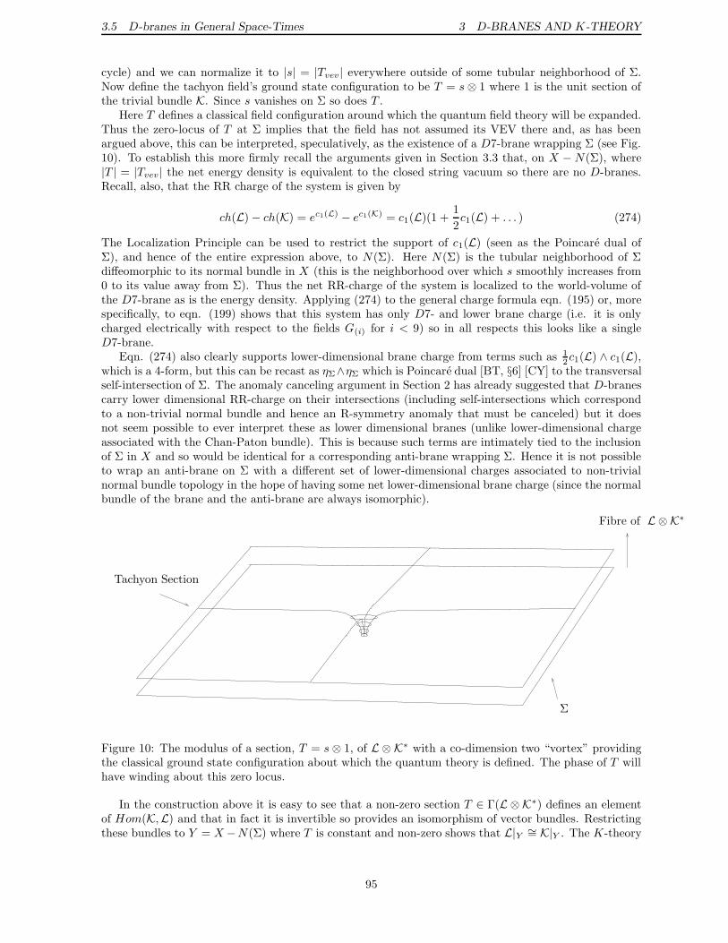
3.5 D-branes in General Space-Times 3 D-BRANES AND K-THEORY
cycle) and we can normalize it to |s| = |Tvev | everywhere outside of some tubular neighborhood of Σ.Now define the tachyon field’s ground state configuration to be T = s⊗ 1 where 1 is the unit section ofthe trivial bundle K. Since s vanishes on Σ so does T .
Here T defines a classical field configuration around which the quantum field theory will be expanded.Thus the zero-locus of T at Σ implies that the field has not assumed its VEV there and, as has beenargued above, this can be interpreted, speculatively, as the existence of a D7-brane wrapping Σ (see Fig.10). To establish this more firmly recall the arguments given in Section 3.3 that, on X −N(Σ), where|T | = |Tvev | the net energy density is equivalent to the closed string vacuum so there are no D-branes.Recall, also, that the RR charge of the system is given by
ch(L)− ch(K) = ec1(L) − ec1(K) = c1(L)(1 +1
2c1(L) + . . . ) (274)
The Localization Principle can be used to restrict the support of c1(L) (seen as the Poincare dual ofΣ), and hence of the entire expression above, to N(Σ). Here N(Σ) is the tubular neighborhood of Σdiffeomorphic to its normal bundle in X (this is the neighborhood over which s smoothly increases from0 to its value away from Σ). Thus the net RR-charge of the system is localized to the world-volume ofthe D7-brane as is the energy density. Applying (274) to the general charge formula eqn. (195) or, morespecifically, to eqn. (199) shows that this system has only D7- and lower brane charge (i.e. it is onlycharged electrically with respect to the fields G(i) for i < 9) so in all respects this looks like a singleD7-brane.
Eqn. (274) also clearly supports lower-dimensional brane charge from terms such as 12c1(L) ∧ c1(L),
which is a 4-form, but this can be recast as ηΣ∧ηΣ which is Poincare dual [BT, §6] [CY] to the transversalself-intersection of Σ. The anomaly canceling argument in Section 2 has already suggested that D-branescarry lower dimensional RR-charge on their intersections (including self-intersections which correspondto a non-trivial normal bundle and hence an R-symmetry anomaly that must be canceled) but it doesnot seem possible to ever interpret these as lower dimensional branes (unlike lower-dimensional chargeassociated with the Chan-Paton bundle). This is because such terms are intimately tied to the inclusionof Σ in X and so would be identical for a corresponding anti-brane wrapping Σ. Hence it is not possibleto wrap an anti-brane on Σ with a different set of lower-dimensional charges associated to non-trivialnormal bundle topology in the hope of having some net lower-dimensional brane charge (since the normalbundle of the brane and the anti-brane are always isomorphic).
PSfrag replacements
Σ
Fibre of L ⊗K∗
Tachyon Section
Figure 10: The modulus of a section, T = s⊗ 1, of L ⊗ K∗ with a co-dimension two “vortex” providingthe classical ground state configuration about which the quantum theory is defined. The phase of T willhave winding about this zero locus.
In the construction above it is easy to see that a non-zero section T ∈ Γ(L ⊗K∗) defines an elementof Hom(K,L) and that in fact it is invertible so provides an isomorphism of vector bundles. Restrictingthese bundles to Y = X −N(Σ) where T is constant and non-zero shows that L|Y ∼= K|Y . The K-theory
95

3.5 D-branes in General Space-Times 3 D-BRANES AND K-THEORY
class associated with this configuration, [L,K], is thus an element of K0(X,Y ) since the bundles L andK are isomorphic on Y .
3.5.3 Incorporating CP-Bundles and Lower-Dimensional Brane Charge
More generally Σ might support a a possibly non-trivial, rank n gauge bundle W → Σ (correspondingto multiple D7-branes wrapping Σ). Such a configuration can carry lower-dimensional brane chargeassociated with topological non-triviality of W and it should be possible to construct an element ofK0(X,Y ) corresponding to these configurations. Assuming, for the moment, that there exists a bundle
W → X which extends W over X , in a way that will be made more precise below, and such thatch(W) = ch(W), then such a D7-brane system can be defined as the decay product of n pairs of D9-
D9-branes with gauge bundles L ⊗ W and K ⊗ W (respectively) where L and K are as defined above.
The extended tachyon field in such a configuration would be a section of L ⊗ W ⊗ K∗ ⊗ W∗ so all thearguments given above still apply, suggesting that T condenses away from N(Σ).61 The RR-charge ofthe system is given by
ch(L ⊗ W)− ch(K⊗ W) =(ch(L)− ch(K)
)ch(W) = c1(L)
((1 +
1
2c1(L) + . . . )ch(W)
)(275)
Once more, localization (of the support of c1(L) = ηΣ) will restrict the support of this charge to a
neighborhood of Σ and so the system looks like a D7-brane wrapped on Σ with RR charge ch(W) =ch(W). The first term (in the last expression) in (275), c1(L)∧ ch(W), is equivalent to ηΣ∧ ch(W) whichis the charge, from (195) or (199), for a D7-brane with world-volume Σ and CP-bundle W . Thus, in this
more general case, the K-theory class defining the D7-brane is [L ⊗ W ,K ⊗ W] ∈ K0(X,Y ).
The explicit construction of W from W is simple in this case (in the more general setting with highercodimension a construction based on the Thom isomorphism for K-theory must be used). First, W is
pulled back to a bundle over N(Σ), W ≡ π∗(W)→ N(Σ), via the projection, π : N(Σ)→ Σ. This gives
two bundles L⊗W and K⊗W (where it is understood that L and K here have been restricted to N(Σ))defined on N(Σ) which might be extendable to X . Even if this is not the case it is possible to considera modification that will still result in the same final D7-brane configuration.
Specifically, invoking Theorem 3.8, consider the bundle Z = (L ⊗ W)⊥ defined so that (L ⊗ W)⊕Zis isomorphic to a trivial bundle over N(Σ). Then, since Y includes the boundary of the closure, ∂N(Σ),and since L|Y ∼= K|Y , the isomorphism restricts to the boundary ∂N(Σ) = N(Σ)−N(Σ) so
(L ⊗ W ⊕ Z)|∂N(Σ)∼= (K ⊗ W ⊕ Z)|∂N(Σ) (276)
Although W has only been defined on N(Σ) it extends uniquely to N(Σ) (because any continuousfunction, including transition functions, extend uniquely onto closures). This isomorphism implies thatboth bundles are trivial on ∂N(Σ) so both can be extended to all of X (simply by defining the extensionto be the trivial bundle of the same rank on Y , which obviously agrees on ∂N(Σ)). Thus the bundles
L⊗W ⊕Z and K⊗W ⊕Z are well defined bundles on all of X and can be used to define a configurationof D9-D9-pairs which will decay into the D7-brane configuration W → Σ. This follows because, oncemore, the pairs are isomorphic on Y so the bundle [L⊗ W ⊕Z ]⊗ [K⊗W ⊕Z ]∗, of which T is a section,admits a constant non-vanishing section on Y (indicating tachyon condensation in this region) and thenet charge of the D9-D9 system is given by
ch(L ⊗ W ⊕ Z)− ch(K ⊗ W ⊕ Z) = c1(L)((1 +
1
2c1(L) + . . . )ch(W)
)(277)
So the final decay product looks exactly the same as that of the simpler case where W extended directlyto a bundle on all of X . The only difference is that here additional pairs of isomorphic yet topologicallynon-trivial pairs of D9-D9-branes (corresponding to Z) had to be added to define the configuration;because the net charge of these additional branes is zero this addition of “virtual” branes violates no
61By construction fW is only defined on N(Σ) and is extended trivially off it (see discussion later). Hence away from
N(Σ) the factors W and W∗ in L⊗ fW ⊗K∗ ⊗ fW∗ are trivial.
96

3.5 D-branes in General Space-Times 3 D-BRANES AND K-THEORY
conservation law. Mathematically this statement follows from the relation [L ⊗W ,K ⊗W ] = [L ⊗W ⊕Z ,K⊗W⊕Z ] and the fact that RR-charge is measured by the Chern homomorphism image of K-theory
classes. The relationship ch(W) = ch(W) and similar equalities for any characteristic classes follows
from the construction of W via the pull-back, π∗, which is an isomorphism on cohomology. Thus, forany codimension two brane in any spacetime and with any embedding topology, this gives a well definedprescription to associate to it a unique element, [L ⊗W ,K ⊗W ] in this case, of K0(X,Y ) (where Y isdefined relative to the D-brane worldvolume).
Note that in (275), L and W , play very different roles. The former defines the world-volume ofthe D7-brane via its zero locus and its first Chern class acts as the Poincare dual of the brane. Thelatter, on the other hand, can only have topological defects on Σ (since it is trivial off Σ and must beisomorphic to a bundle defined on Σ) and these defects can conceivably develop into lower-dimensionalbranes (for instance by placing a sufficient number of anti-branes on Σ with trivial CP bundles). If alllower-dimensional branes occurred like this it would be possible to simply use this construction iteratively.To define a Dp-brane with p+ 1 dimensional worldvolume Σp we could apply the above prescription to
generate a set of D(p+ 2)-D(p+ 2)-pairs wrapping some cycle Σp+2 (nothing in the above constructionconstrained it to D7-branes defined via D9-D9-pairs; any codimension two configuration will work) suchthat Σp ⊂ Σp+2 and repeat iteratively until Σp+2k = X for some iteration k. This is not possible,however, for a general Σp since the chain of embeddings Σp ⊂ Σp+2 ⊂ . . . ⊂ X is not always guaranteedto exist. Thus a more general construction must be invoked that works for any codimension. It will turnout that the codimension two case is a special case of this more general construction.
3.5.4 The Thom Isomorphism in K-Theory
In codimension two we used the Poincare dual to Σ to construct, explicitly, a line bundle, L, withsections vanishing on Σ which could be tensored with an arbitrary bundle, W , so that the product couldbe extended all over X to define a configuration of D9-D9-branes with the same RR-charges and energydensity as a D7-brane on Σ with CP bundle W . For higher codimension it is not generally possible todefine the analog of L using only the Poincare dual of Σ. Rather, a construction from K-theory, theK-theoretic Thom isomorphism [Kar], [OS], [LM], can be used to directly construct a K-theory class(corresponding to a pair of bundles) that plays the same role as the Thom class in cohomology (recall,from Proposition 2.4, that the Poincare dual is the Thom class of the normal bundle of a submanifold).That is, a pair of bundles, defined on the normal bundle, NΣ, whose K-theory class has compact supportin the vertical direction (i.e. the pair are isomorphic outside of some compact subspace of the bundle)and which is also a generator of the compact K-theory of the bundle, K0
cpt(NΣ). By K0cpt(NΣ) we
essentially mean the relative K-group K0(B(NΣ), S(NΣ)) where B(NΣ) and S(NΣ) are the ball andsphere bundles associated to NΣ (see below). The fact that this class is a generator of the K-group isanalogous to the fact that the cohomological Thom class is the generator of the compactly supported (inthe vertical direction) cohomology of a vector bundle since it is a bump function which can be integratedvertically (along the fibers) to give the value one (see Section 2.6.3).
The construction of theK-theoretic Thom class, as this class is known, is rather technical and has beendeferred to Appendix B.1 (also see [LM], [Kar] for more details and proofs). We highlight the essentialdefinitions here. Consider a real vector bundle π : N → Σ (which will correspond to the normal bundle inour construction) where N is of dimension 2k and admits a spin-structure (this, and the generalizationto a Spinc-structure, are discussed in the Appendices). Associated to N are two bundles, B(N) ⊂ Nand S(N) ⊂ N , which are the ball and sphere bundle, respectively, whose fibers are the 2k-dimensionalball and and the 2k− 1-dimensional sphere, B2k, and S2k−1 = ∂B2k. Note that the former is homotopicto the base space Σ (and to N itself) since each fiber is contractable so there is an induced bijectionV ect(Σ) ∼= V ect(B(N)) (∼= V ect(N)) defined by the pull-back via π : B(N) → Σ (π is the restriction ofπ : N → Σ to B(N) ⊂ N ; we will be sloppy and denote them both using the same symbol).
In Appendix B.1 the Thom class in K-theory for the bundle N is constructed in terms of the complexSpin-bundles, S±(N), associated to N . These are pulled back to B(N) via π : B(N) → Σ and a bundlemorphism, α : π∗(S+(N)) → π∗(S−(N)), is defined that restricts on the boundary, S(N) = ∂B(N), toan isomorphism which is homotopically non-trivial. This defines a class,
U = [π∗(S+(N)), π∗(S−(N));α] ∈ K0(B(N), S(N)) (278)
97

3.5 D-branes in General Space-Times 3 D-BRANES AND K-THEORY
which is trivial outside of a compact subspace of each fiber of N . Assuming Σ is, itself, compact then Ucorresponds to a class in K0
cpt(N).62 If Σ is not compact the class U is not well-defined but can still beused to give a well-defined product (281) below (see [Kar, IV.5] or [LM, App. C]). We denote this class
UN = [π∗(S+(N)), π∗(S−(N))] ∈ K0cpt(N) (279)
The notation here is somewhat sloppy since we have dropped the dependence of the class on the thebundle morphism α (because classes in compact K-theory are given by pairs of bundles, not a pair and amorphism). In relativeK-theory there might be several different classes associated to the pair π∗(S+(N))and π∗(S−(N)) but since we know we are referring to the Thom class which is defined with a particularmorphism α (defined to have winding number one on the boundary, S(N)) we will just be lax about this.More details can be found in the Appendix B.1.
In the sequel we will discuss only K0cpt(N) and K0(Σ) whether Σ is compact or not assuming, in all
cases, that compactly supported K-theory is used (Σ is always locally compact). The relevance of UN isthat it can be shown to be a generator of the group K0(N) [Kar, IV].
Theorem 3.9 (Thom Isomorphism (in K-theory)). For a real 2k-dimensional bundle N → Σ, witha Spinc-structure, the product with UN ∈ K0
cpt(N) induces an isomorphism
K0(Σ) ∼= K0cpt(N) (280)
Moreover, the group K0cpt(N) is a free K0(Σ)-module63 with generator UN .
More concretely this means that any element, ν ∈ K0(N), can be written as
ν = π∗(λ) ~ UN (281)
for some λ ∈ K0(Σ). Since K0(N) is a free module (of rank 1) over K0(Σ) the two groups are isomorphicK0(N) ∼= K0(Σ). The isomorphism maps any element of K0(Σ) to an element of K0(N) by the pull-backof the projection, π, followed by multiplication with UN as given above.
To make sense of this statement it is first necessary to understand what it means that K0(N) is aK0(Σ)-module. Recall that a module is an Abelian group admitting an action given by a homomorphismfrom K0(Σ) ×K0(N) to K0(N). For example, for a Lie group, G, with a representation, V , there is amap (g, v) 7→ g · v ∈ V . In this case the homomorphism is given by composing the maps
K0(Σ)×K0(N)⊗−→ K0(Σ×N)
K0(Σ×N)(π×id)∗−−−−−→ K0(N)
(282)
The second map is simply the pull-back of the proper map π × id : N → Σ × N while the first map,⊗, is much more involved. Given λ = [W ,V ;β] ∈ K0(Σ) where β is an isomorphism outside a compactneighborhood (if Σ is not compact) and UN as defined above64 the product, ⊗, is given by [LM]
ν = λ⊗UN ≡ [v1, v2; ρ]
v1 = (W π∗(S+))⊕ (V π∗(S−))
v2 = (V π∗(S+)⊕ (W π∗(S−))
ρ =
(β 1 −1 α∗
1 α β∗ 1
)
(283)
62B(N)/S(N) is topologically the one-point compactification of N .63A module is essentially a representation of a ring, R. A free R-module, F , is a module that is isomorphic to a number
of copies of the ring so F ∼=LN
i=0 R. See also discussion below.64The product, ⊗, is a well defined product for any two spaces, Σ and N , and any of their K-theory classes, not only
the Thom class, UN , of a bundle, N . We use this particular example here because it will be useful later in the discussion.Hopefully this will not cause confusion.
98

3.5 D-branes in General Space-Times 3 D-BRANES AND K-THEORY
Note here the pretense of π∗(S±) instead of just S± is an artifact of how UN was defined and is not relatedto the definition of the product ⊗. Above and in the sequel we will be somewhat sloppy in differentiatingbetween the bundle S±(N) and its fibers, S±, since the context will generally make it clear which isintended. The symbol denotes the outer tensor productWπ∗(S+) ≡ (π∗
1(W))⊗ (π∗2(π∗(S+))) where
π1 : Σ × N → Σ and π2 : Σ × N → N are projections onto factors. Thus the statement of the Thomisomorphism for K-theory is that, under the action of K0(Σ) on K0(N) just defined, K0(N) is a freemodule with its K-theoretic Thom class, UN , as the generator.
3.5.5 Examples and Remarks
To gain an intuitive sense for this rather technical construction let us see exactly what this means for avector bundle W → Σ. This vector bundle can be used to define an element of K0(Σ), namely [W , In]where In is the trivial rank n bundle over Σ and n is the rank of W . Now consider the image of thisbundle under the isomorphism, K0(Σ) ∼= K0
cpt(N) described above
[W , In] 7→[(π∗(W) π∗(S+))⊕ (π∗(In) π∗(S−)),
(π∗(W) π∗(S−))⊕ (π∗(In) π∗(S+))]∈ K0
cpt(N)
The image of [W , In] is more cleanly represented as
[π∗(W) π∗(S+), π∗(W) π∗(S−)
]+[π∗(In) π∗(S−), π∗(In) π∗(S+)
](284)
So the relative bundle W → Σ has been extended to a bundle over N with compact support by tensoringit with both π∗(S+) and π∗(S−) which are isomorphic to each other outside of a compact neighborhoodof N homotopic to Σ (i.e. the origin in each fiber). That is to say, both classes above are trivial outsideof some compact region corresponding to the region where α : π∗(S+) → π∗(S−) is an isomorphism.This is exactly the point of the Thom isomorphism. Namely to extend a bundle W on Σ represented bya K-theory class [W , In] to a bundle on N which has compact support in the vertical direction. Noticethat one might also consider a more trivial isomorphism given by the map (W , In) 7→ (π∗(W), π∗(In))via the pull-back of the projection (that this is a bijection follows from the fact that the total space of Nis homotopic to Σ) but these bundles no longer have compact support in N so will not extend to globalelements in X .
It is also instructive to consider the relationship between the K-theoretic Thom isomorphism and thecohomological one. In both cases an object defined on a manifold, Σ, is lifted to an object defined on abundle N → Σ over that manifold; since, in both cases, the objects are sensitive only to the homotopytype of the base space and since any vector bundle, N , is homotopic to Σ this lifting is an isomorphism.In cohomology the Thom class, Φ(N), of the bundle is a form with compact support in the verticaldirection and is the image of 1 ∈ H0(Σ) under the cohomological Thom isomorphism. Thus, under theisomorphism, Φ(N) restricts to the generator of compactly supported cohomology on the fiber. Likewise,the K-theoretic Thom class defined above, UN , is shown [LM] to be the generator of the compactlysupported K-theory of the fibers of N .65 Let us consider the image of the Thom class, UN , under theChern homomorphism between K0
cpt(N) and Heven(N,Q)
ch(UN ) = ch([π∗(S+(N)), π∗(S−(N))]) ≡ ch(π∗(S+(N)))− ch(π∗(S−(N)))
= π∗(ch(S+(N))− ch(S−(N))) = π∗
(e(N)
A(N)
)
= π∗((A(N))−1
)π∗(s∗0(Φ(N))) = π∗
((A(N))−1
)∧ Φ(N)
(285)
Where we have recalled that the Euler class is the pullback of the Thom class via the zero sections0 : Σ → N and have applied eqn. (78). A slight subtlety that is being neglected in this equation isthat π∗ is only an isomorphism onto normal cohomology not cohomology with compact vertical support;
65A quick way to see this is that the compactified fibers are topologically Sn and the Thom class in K-theory is definedvia a pair of bundles, π∗(S±(N)) which are isomorphic on the equator, Sn−1, via an isomorphism of winding number one.Recall that all vector bundles on Sn are classified by their winding number along the equator.
99

3.5 D-branes in General Space-Times 3 D-BRANES AND K-THEORY
thus the class Φ(N) should be seen as a class in H•(N,Q). Thus the image of the K-theoretic Thomclass differs from the Cohomological Thom class by the inverse of the roof-genus of the normal bundle.We will show in the next section that this contribution gives a very natural interpretation to the chargeformula for a D-brane, (195). Namely, instead of being the push-forward of a cohomology class on Σassociated to W , eqn. (195) should be interpreted as the K-theoretic push forward of the K-theoryclass associated with W (as in our construction above). Before going on to use the K-theoretic Thomisomorphism to define D9-D9 configurations, as promised, let us first make a few more observations aboutthis construction that relate it to things we have already seen.
Although the construction of the Thom isomorphism might seem somewhat abstract we have, in fact,already undertaken it by hand for some special cases. The first is the codimension two construction in thegeneral topological setting discussed in the Section 3.5.2. To understand to relation between the Thomisomorphism and the cohomological construction of a line bundle requires using some results from therepresentation theory of Clifford Algebras related to the construction of the Thom class (see AppendixB.1). The interested reader should consult Appendix B.2. The construction presented here can also beseen as a general case of the construction used for trivial normal bundlesNΣ ∼= R10−2k×B2k in Section 3.4.There, pairs of bundles where considered that were isomorphic on the boundary ∂NΣ = R10−2k×S2k−1.These bundles were fixed by their winding number from S2k−1 to U(n) for n the rank of the bundle.Although it is not immediately evident, this does, in fact, coincide with the construction above sinceα is required to be an isomorphism on S(N) which looks locally like Σ × S2k−1. By construction theisomorphism α restricts to the generator of π2k−1(U(n)) for n = 2k−1.
3.5.6 RR Field Equations and the Thom Isomorphism
Although we have already spent considerable effort developing the Thom isomorphism for K-theory, andhave connected it to some earlier constructions, all we have, by way of motivation, is the geometricintuition that it can be used to extend K-theory classes from Σ to X . Let us now see if this constructioncan be motivated by appealing directly to the RR field equations. Starting with the charge formula inH•c (X)
d ∗G = µ∑
i
ηΣi∧ π∗
(ch(W) ∧
√A(TΣ)
A(NΣ)
)(286)
and pulling it back to Σ using ι∗(ηΣ) ≡ ι∗(Φ(NΣ)) = e(NΣ) and A(ι∗(TX)) = A(TΣ)A(NΣ) whereι : Σ→ X is the embedding, this can be re-written as
ι∗(d ∗G) = µ∑
i
(ch(W) ∧ e(TΣ)
A(NΣ)
)∧√A(ι∗(TX))
= µ∑
i
(ch(W) ∧ (ch(S+(NΣ))− ch(S−(NΣ)))
)∧√A(ι∗(TX))
(287)
The second line follows from the identity, used in Section 2, that holds for any spin, orientable vectorbundle E
ch(S+(E))− ch(S−(E)) =e(E)
A(E)(288)
Recall that the Chern character defines a homomorphism between K-theory and rational (Cech) coho-mology
ch : K0(X)→ Heven(X,Q)
ch([W ,V ]) 7→ ch(W)− ch(V)(289)
100

3.5 D-branes in General Space-Times 3 D-BRANES AND K-THEORY
Using the definitions of the Chern character and K-theory it is easy to see that this is indeed a homo-morphism. Moreover, if K0(X) is tensored with Q which effectively removes any torsion66 subgroups,then this can be shown to be an isomorphism (see [Kar, Thrm V.3.25] and references therein)
ch : K0(X)⊗Q∼=−→ Heven(X,Q) (290)
It is also possible to define a natural bilinear pairing on each space given by
⟨[W ,V ], [W ′,V ′]
⟩K≡ indDW−V · indDW′−V′
⟨ω, α
⟩dR≡∫
X
ω ∧ α(291)
Where the index of a difference bundle, [W ]−[V ], is defined to be the difference of the indices indDW−V ≡indDW − indDV . indDW is the index of the Dirac operator on X twisted by a bundle W (see [Nak] forthis terminology). The Chern character, as given, above does not preserve this bilinear form but it iseasy to see that a modified version does [MM]
ch : K0(X)⊗Q→ Heven(X,Q)
ch([W ,V ]) 7→ (ch(W)− ch(V)) ∧√A(TX)
(292)
Under this modified isomorphism the last line of (287) appears as the image of [π∗(W)⊗π∗(S+), π∗(W)⊗π∗(S−)] pulled down to Σ. We observe, therefore, that the RR field equations are themselves verysuggestive of the K-theoretic Thom isomorphism. This argument is based primarily on the presence ofthe term e(NΣ)/A(NΣ) in eqn (287) and is not so reliant on the (perhaps arbitrary) choice of bilinearpairing defined above (i.e. the modified Chern homomorphism is required to get an exact match withequation (287) but even without it, the presence of the term e(NΣ)/A(NΣ) is suggestive of the K-theoretic Thom isomorphism).
3.5.7 Lower Dimensional Branes and the Thom Isomorphism
The techniques introduced in Section 3.5.4 can now be used to generalize the construction of a D7-braneconfiguration to configurations of lower dimensional branes. It is important in defining this constructionto recall that the equivalence between Dp-branes and configurations of D9-D9-brane pairs is based onthe fact that the two systems have the same conserved charges, both in terms of the RR-field strengthsand energy density. Thus in specifying a configuration of D9-D9-pairs which we expect to decay into aDp-brane we are constrained only by the total charges in both systems.
Let us now consider a Dp-brane for p odd (since we are in IIB) on a world-volume Σ with a Chan-Paton bundle W → Σ. This information encodes all the charges of the system since the RR-charge isgiven by the formula (195) and the energy density is a constant function (whose value is fixed by thevalue of p via the D-brane tension, τp) on the world-volume Σ. Recall, also, that on a D9-D9 system theenergy density can be related to the tachyon, seen as a section of tensor product of Chan-Paton bundles,via equation (232) which implies that wherever this section has a value coinciding with the tachyon VEVthe local energy density is equivalent to the closed string vacuum. Thus there is a non-vacuum energydensity, coinciding with a putative Dp-brane worldvolume, on the zero-locus of the tachyon section.
With this introduction we hope to have motivated the following construction. The general programwill be, following [Wit2], to define a Dp-brane wrapping Σ with a CP-bundle W as a K-theory class inK0(X) with some compactness condition (in transverse directions) by first pushing the class of W intoa class in K0(N) via the Thom isomorphism and then extending that to a class in K0(X) with compactsupport. This general theme has already been pursued several times, first for cohomology classes inSection 2, and then for line bundles in the last few subsections. The bundle associated to W in K0(X)will be the pullback of W onto the normal bundle tensored with spinor bundles π∗(S±) associated to the
66A torsion group is a group with a nilpotent generator such as Z2. The tensor product, over Z, of a torsion group withQ will always be zero since any element of the tensor product will be equivalent, via the tensor relations, to zero. Consider1 ⊗ p
q∈ Zn ⊗Z Q for any p, q ∈ Z. Then, under the tensor product, this is equal to 1 ⊗ np
nq= n⊗ p
nq= 0 ⊗ p
nq= 0.
101

3.5 D-branes in General Space-Times 3 D-BRANES AND K-THEORY
normal bundle as described in Section 3.5.4. The physical interpretation of this will be that the extendedspinor bundles π∗(S±) defined on all of X and viewed as complex, rank n, vector bundles (but alsocarrying additional algebraic structure) are actually the CP bundles of the D9-D9-pairs. This invertsthe usual logic where we define Chan-Paton bundles associated to D9-D9-pairs and then declare that thezero-locus of a generic section of such a bundle is the world-volume of a lower-dimensional brane. Herethe world-volume is already given and, via the Thom isomorphism, it is possible to construct bundleswith the correct generic zero-loci. In addition, lower-dimensional brane charge is encoded in W → Σwhich then multiplies π∗(S±) to define spacetime filling brane configurations that encode, not only theembedding of Σ, but also the lower dimensional brane charge of its CP-bundles.
Let us work this out in detail. Let Σ now be the world-volume of a Dp-brane (p odd), π : NΣ → Σits even dimensional normal bundle, and W → Σ its Chan-Paton bundle (which may be the trivial rank1 bundle, I1, for a single brane without any lower dimensional brane charge). We assume that Σ isconnected (see below) but this is not a serious limitation since the K-theory of disjoint unions is easilycalculated from the K-theory of each connected component (one can define a Dp-brane to be a connectedcomponent and then treat a disconnected Σ as multiple Dp-branes). We also assume Σ is compact or, ifit is locally compact, we work on its (one-point) compactification so its K-theory is well-defined. Now wewant to define a map V ect(Σ) → K0(Σ) by fixing a bundle V → Σ and defining the map W 7→ [W ,V ].It is necessary to fix a V in order to define an inclusion of V ect(Σ) into K0(Σ), its Grothendieck group,and this will have the physical interpretation of defining the “zero-charge” of Dp-branes.
We want to push this K-theory class in K0(Σ) to a class in K0(X,Y ), where the use of relative K-theory ensures that the image of the class is trivial on the complement of N(Σ), namely Y = X −N(Σ).This is done using the K-theoretic Gysin map (see [Kar]) which is essentially the Thom isomorphism,used to mapK0(Σ) intoK0
cpt(NΣ), followed by an extension of the classK0cpt(NΣ) to a class in K0(X,Y ).
This is analogous to the cohomological Gysin map which was used in Section 2 to push forward elementsof cohomology from H•(Σ) to H•(X). Note that, to apply the Thom isomorphism, we must assume thatNΣ is a spin-bundle. If this is not true a slight modification is required that will be addressed in the nextsection. Another point to note is that the Gysin map, as defined above, requires that Σ be embeddedinto X so that there exists tubular neighborhood, N(Σ), diffeomorphic to the normal bundle, NΣ. In[Kar, Ch. IV, §5] it is shown, however, that any proper, continuous map ι : Σ→ X for which the inducednormal bundle has a Spinc-structure can be used to define a Gysin map, ι∗ : K0(Σ) → K0(X). We willrestrict the discussion here to the case of an embedding but using the above mentioned theorem it is clearthat this can be generalized to the case where Σ is not a submanifold of X .
Explicitly then, the class [W ,V ] ∈ K0(Σ) is mapped to the class in K0cpt(NΣ) given by (284)
[π∗(W)⊗ π∗(S+), π∗(W)⊗ π∗(S−)
]+[π∗(V)⊗ π∗(S−), π∗(V)⊗ π∗(S+)
]=
[π∗(W)⊗ π∗(S+), π∗(W)⊗ π∗(S−)
]−[π∗(V)⊗ π∗(S+), π∗(V)⊗ π∗(S−)
]=
(293)
By construction, we know that these classes are trivial on the boundary of the tubular neighborhood,N(Σ) (since there π∗(S±) are isomorphic), which we will denote ∂N(Σ)
(π∗(W)⊗ π∗(S+)
)|∂N(Σ)
∼=(π∗(W)⊗ π∗(S−)
)|∂N(Σ)(
π∗(V)⊗ π∗(S−))|∂N(Σ)
∼=(π∗(V)⊗ π∗(S+)
)|∂N(Σ)
(294)
We would like to extend these bundles, defined on N(Σ) ⊂ X , to all of X but this may not alwaysbe possible for topological reasons. If not, we proceed as in the case of a line bundle. First, we apply
Theorem 3.8 to demonstrate the existence of a bundle Z =(π∗(W)⊗ π∗(S+)
)⊥such that
(π∗(W)⊗ π∗(S+)) ⊕Z ∼= Im (295)
for some m (and likewise find a Z ′ for π∗(V)⊗ π∗(S−)) and then use
[π∗(W)⊗ π∗(S+), π∗(W)⊗ π∗(S−)
]=[π∗(W)⊗ π∗(S+)⊕Z , π∗(W)⊗ π∗(S−)⊕Z
](296)
102

3.5 D-branes in General Space-Times 3 D-BRANES AND K-THEORY
because they define the same K-theory class. Since π∗(W)⊗π∗(S+)⊕Z is trivial, and it is isomorphic toπ∗(W)⊗ π∗(S−)⊕Z on the boundary, ∂N(Σ), both bundles can be extended trivially over all of X (byjust gluing to the trivial bundle defined on Y = X −N(Σ)) giving a class in K0(X,Y ). This is exactlythe same procedure as undertaken in Section 3.5.2 with respect to line bundles.
We now associate to this configuration, W → Σ, only the first class in this sum,
[π∗(W)⊗ π∗(S+)⊕Z , π∗(W)⊗ π∗(S−)⊕Z
](297)
This is a consistent choice because we define the class of the configuration to be its image under the Gysinmap minus the class
[π∗(V)⊗ π∗(S+), π∗(V)⊗ π∗(S−)
]. The choice is consistent because we defined the
map from V ect(Σ) to K0(Σ) using the bundle V and it is easy to check that, after subtracting thiscontribution, the final class in K0(X) corresponding the the Dp-brane configuration no longer dependson the choice of V . Physically one can think of V as a “zero-point” background charge against whichother charges are measured. One also easily checks that, with respect to the Dp-brane charge formula,eqn. (287), this is the correct prescription.
In order to complete the construction it remains to define a configuration of D9-D9-brane pairs fromthe data we have so far. To do this we will have to use some simple results from the representation theoryof Clifford Algebras (see [LM, I.5] and Appendix B). First, note that the bundles S± have fibers S±x(x ∈ Σ) which are complex vector spaces of complex dimension 2k−1 where the dimension of N is 2k.The transition functions for these bundle are SpinC(2k) ⊂ GL(2k−1,C) valued (in fact they correspondto the two irreducible representations of SpinC(2k)) and we would like to use these to treat S± as 2k−1-dimensional complex vector bundles that we can declare to be (part of) the Chan-Paton bundles of theD9-D9-brane pair. Recall that such a bundle must be of the form W ⊗ V∗ where W and V are equalrank complex vector bundles and here the minimum rank suggested is 2k−1 corresponding to the complexdimension of the fibers S±x . Observe that such a bundle requires the same number of D9-D9-brane pairsas does the step-wise iterative construction, described at the end of Section 3.3.6, which can be appliedwhen a suitable embedding of cycles exists.
To complete the construction above we want to show that the bundles S± have unitary transitionfunctions (i.e. valued in U(2k−1)). Normally any complex vector bundle admits a reduction to a uni-tary structure group but this assumes the freedom to reduce the structure group using any elements ofGL(2k−1,C) not only elements of the subgroup SpinC(2k). Thus, in this case, it is necessary to showthat the SpinC action is, itself, unitary. This follows from a proposition in [LM, Prop. 5.16] showingthat the complex representation of SpinC are unitary (or can be made unitary). Starting with a fixedinner product on S± it is possible to define a new one as follows. First, define a subgroup of the CliffordAlgebra C(R2k) that is finite and then define a new inner product by averaging over the action of thissubgroup. This is a standard construction which can be used to construct an inner product for whicha given representation of a compact (or finite) group is unitary. Under this new inner product the rep-resentation of the Spin subgroup will also be unitary. Thus the action of the SpinC valued transitionfunctions of S± on these bundles can be made unitary which means they are complex vector bundles inthe fundamental of U(2k−1).
3.5.8 Normal Bundles with Spinc Structure
We have thus far assumed that the bundle NΣ admits a spin-structure, meaning that its second Stiefel-Whitney class vanishes. This was necessary in the Thom isomorphism because it allowed for the con-struction of Spin-bundles lifted from N which define the Thom class of the normal bundle. The notionof Spinc has already been mentioned in Section 2.7 and is discussed in some depth in Appendix A so wewill be brief here. We will assume the reader is familiar with the content of these sections so the readerwho has skipped them should also feel free to skip this section as well as it mostly concerns technicaldetails that do not significantly alter the argument.
Recall that in [FW] it was shown, by analyzing a global anomaly on the string worldsheet theory, thatthe normal bundle of a D-brane must always admit a Spinc structure if the B-field has a topologicallytrivial field strength (which has been the assumption so far). Thus even if N does not lift to a Spinbundle, meaning that the bundles S± do not satisfy the cocycle condition and are not well defined, thereexists a line bundle, L, on Σ whose “square-root” bundle L1/2 fails to satisfy the cocycle condition in the
103

3.6 Conclusions 3 D-BRANES AND K-THEORY
same way as S± so that the tensor product bundles, S± ⊗ L1/2, are well-defined. This can be used inthe construction of the Thom class to define it as [π∗(S+ ⊗L1/2), π∗(S− ⊗L1/2)].
As demonstrated in [FW] and discussed in Section 2.7, the line bundle L1/2 is actually the Chan-Paton bundle of a single D-brane and, if NΣ is Spinc but not Spin (i.e. w3(NΣ) = 0 but w2(NΣ) 6= 0),then this bundle is not well defined as it does not satisfy the cocycle condition. Even for the case of anAbelian Chan-Paton bundle (a single brane) there is an ambiguity regarding exactly what the definitionof the Spinc component is. This was discussed under eqn. (174) and comes from the ability to factor
L1/2 into two parts, Z and Z , the first of which enters the D-brane charge formula, eqn. (185), as theactual gauge bundle (W in that formula) of the D-brane and the second of which gives the Spinc-factor(ed/2 in that formula). It is obvious, however, from the construction of the Thom isomorphism andits relation to Theorem 2.10 (see Section 2.8) that this splitting has no effect on the resultant D-branecharge or K-theory class. Consider the image of the CP-bundle L1/2 under the Thom isomorphism whereL1/2 ∼= Z⊗Z and Z has a “half-integer” Chern class and so defines a Spinc bundle. Then the Thom classwould be given by [π∗(S+ ⊗ Z), π∗(S− ⊗ Z)] and the Chan-Paton bundle is considered the well-definedfactor, Z (i.e. the factor with an integer Chern class). The image of Z (or [Z ,V ]) under the Thomisomorphism is
[π∗(Z ⊗ S+ ⊗ Z), π∗(Z ⊗ S− ⊗ Z)] (298)
which is just
[π∗(L1/2 ⊗ S+), π∗(L1/2 ⊗ S−)] (299)
and so is entirely independent of the factorization, L1/2 ∼= Z ⊗ Z, of the Chan-Paton bundle into a“gauge” and a Spinc-bundle.
The use of Spinc-bundles instead of Spin bundles does not affect the rest of the construction of theThom isomorphism or its use in defining D9-D9-configurations corresponding to a D-brane on a world-volume Σ with Chan-Paton bundle W . The arguments of [FW] only strictly apply in the Abelian casewhere the Chan-Paton bundle is a line bundle but we will not attempt to deal rigorously with the moregeneral case until the next section. As noted in Section 2.7 the more general analysis of Spinc suggests thatthe bundle W is a twisted vector bundle that does not satisfy the cocycle condition by a Z2 factor (whichis also true of L1/2 above). Thus one might imagine a simple extension of the arguments above to themore general case where the twisted line bundle, L1/2, is given by the determinant bundle L1/2 ≡ det(W).
3.6 Conclusions
Our analysis has provided an elegant geometric understanding of exactly why D-branes are classified byK-theory, at least in the simplified setting to which we’ve restricted ourself (no background B field). Ofcourse the fact that D-brane charges are classified by K-theory was, in some sense, already evident at theend of Section 2. It followed from the identification of D-brane charge as an element of rational K-theoryvia the modified Chern isomorphism (292).
In geometrising the analysis we have gained more than just elegance. The identification of D-branecharge with rational K-theory is insensitive to torsion classes since K0(X) must be tensored with Q.By making a direct connection between D-branes and K-theory using Sen’s construction it is clear thatthe actual D-brane charge is given by the full K-theory class, not just its image in cohomology. Thisof course brings up the issue of when the two differ and of how much relevance the difference betweenrational cohomology and K-theory is for our physical understanding. There is a nice discussion of thesorts of situations in which the exact K-theoretic understanding is important in [MMS]. Specifically, theynote there that it is possible to have a brane wrapping a homologically stable cycle, Σ, yet be unstablebecause of K-theoretic considerations.
The most straightforward consequence of this analysis is simply that, to determine the stability ofa configurations of D-branes, one must consider the class of the branes in the correct K-groups. Moreinterestingly it turns out that the RR field-strengths are, themselves, also classified by K-theory [MW].This is not so surprising since they are generated by sources classified by K-theory but it also turnsout to be very natural in dealing with the fact that they are self-dual. This has led to ongoing work
104

3.6 Conclusions 3 D-BRANES AND K-THEORY
on quantizing theories with such objects, a problem which is sensitive to their geometric nature. Thisproblem is also being studied in M-theory [DMW] where it is being used to better understand the theory.
In the next section we will finally lift the constraint B = 0 and suggest how this effects the analysisand introduces complications whose resolution is not entirely clear (as far as the author is aware). It isthese open problems that make this field tantalizing as they suggest that their resolution might providemore insights into a non-perturbative formulation of string theory or might provide some more insightinto the low-energy approximation to M-theory.
105

4 THE B-FIELD AND TWISTED VECTOR BUNDLES
4 The B-field and Twisted Vector Bundles
So far the discussion in this thesis has been limited to a very special regime in string theory where wehave taken the limit α′ going to zero and set the value of the background antisymmetric tensor field, Bµν ,to zero. Ultimately, we would like to extend our results to a more general setting. In the particular casewhere Bµν 6= 0 and the cohomology class of its field-strength, [H ], is a torsion class this can be done [Kap][Wit2] and suggests that D-branes should, more generally, be classified using twisted K-theory [DK].
The case of a non-torsion [H ] is more speculative [BM] [BCM+] and suggests a possible generalizationto (C∗-)algebraic or other kinds of K-theory. Even more generally, the idea that there is a generalizationof K-theory that applies when the point-limit (α′ → 0) of strings is not taken is an interesting one thathas only been recently studied [TS] [Sch].
Unfortunately, constraints of time and space do not allow us to develop the notions of twisted K-theory (or its variants) in this thesis. Rather we will focus on the physical derivation of the twistedcocycle condition of the CP bundles when H is non-trivial. This twisting implies the analysis of Sections2 and 3 must be modified and ultimately leads to some of the open problems in the field. We offerthis section as a brief enticements and encourage the interested reader to further pursue the referencesstarting with [BM] [BCM+] [Kap] [AS2] [CJM].
4.1 Overview
In this section we will determine how the analysis of Sections 2 and 3 must be modified in the presence of anon-trivial background B-field with a torsion class [H ] ∈ Tor(H3(X,Z)). Recall, from Section 2.4.3, thatopen string modes for strings ending on a D-brane with world-volume, Σ, were shown to be sections of avector bundle Vadj → Σ in the adjoint representation67 of U(N). In that section, we claimed that, whenB = 0 or when it is topologically trivial, the bundle Vadj was equal to W ⊗W where W → Σ is a vectorbundle in a fundamental representation of U(N). We also claimed that on the D-brane world-volumethere is a field, Aµ, generated by the open string modes, that acts as a connection on the Chan-Patonbundle, W → Σ defined in Section 2.4.3.
To understand how Bµν and Aµ are related and when Vadj factors to well-defined bundles, W andW ,requires analyzing the original string world-sheet theory given by the action (5). This action is modified,for an open string, by including the holonomy of a background Aµ field [Pol1]. We write the path integralmeasure schematically as
W [ξ] = F [ξ] · pfaff(iDξ) · exp
(i
∫
∂M
ξ∗(A)
)· exp
(i
∫
M
ξ∗(B)
)(300)
where ξ : M → X is map of the string world-sheet, M , into spacetime, X . W [ξ] is the exponentiated formof the action so the path integral would be given by integrating W [ξ] over the space,M = Map(M,X),of inequivalent maps.68 The factors in its definition will be explained in due course.
In general, holonomies of gauge fields, such as A and B, are well-defined (gauge-invariant) quantitiesso long as they are taken over spaces with no boundaries [Alv]. For closed strings the world-sheet,M , has no boundary so the term Hol∂M (ξ∗A) vanishes and the term HolM (ξ∗B) is well-defined. Foropen strings, however, Hol∂M (ξ∗A) does not vanish but is a well defined quantity while HolM (ξ∗B) isno longer gauge invariant [GR][Gaw]. Since HolM (ξ∗B) is a factor in W [ξ] the latter also becomes ill-defined. We will suggest, below, how to make this vague notion more rigorous. Essentially, if we attemptto consider HolM (ξ∗B) as a function on the space of maps, M, we find that it depends upon a choiceof “coordinates” in this space and, as such, is not really a well-defined function but rather a section of aline bundle, LB →M. This implies that, in this case, W [ξ] also becomes a section of a line bundle onM and hence can only be integrated if that line bundle is trivial.
It is this last observation that introduced a dependence of the gauge field, A, on the background B-field. To makeW [ξ] a well-defined functional we must modify A in such a way that the factor Hol∂M (ξ∗A),rather than being a well-define functional on the spaceM, becomes a section of a non-trivial line bundle,LA, on M. This second line bundle is chosen in such a way that the tensor product LA ⊗ LB , of which
67Or some variation of Vadj in the presence of other branes or anti-branes.68Neglecting for now the need to include the world-sheet metric in the moduli space. The factors that will concern us
are, in any case, independent of the world-sheet metric as they are holonomies of forms.
106

4.1 Overview 4 THE B-FIELD AND TWISTED VECTOR BUNDLES
W [ξ] is a section, is a trivial bundle. This will require modifying the cocycle condition on W → Σ, theChan-Paton bundle on the D-brane, on which A is a connection to be
gαβgβγgγα = eiKαβγ (301)
where eiKαβγ is an element of H2(Σ,Cont(U(1))) related to the (restriction to Σ of the) class of [H ]Σ ∈H3(Σ,Z) in such a way that, as remarked in Section 2.4.3, it will only be possible to set eiKαβγ = 1 whenthe class of [H ] is trivial.
The argument given above only holds when the class [H ], restricted to Σ, is a torsion class, [H ]Σ ∈Tor(H3(Σ,Z)) meaning that its image in de Rham cohomology, H3
dR(Σ) ∼= H3(Σ,R), vanishes. We willshow that the torsion degree of [H ] is related to the rank of W , the putative vector bundle, on which weattempted to define the connection, A. If this bundle is of rank n then n[H ] = 0 so [H ] must be of degreem where m is a divisor of n.
The failure of W [ξ] to be a well-defined function on M would generate a global or non-perturbativeanomaly in the string world-sheet theory known as the Freed-Witten anomaly [FW]. A similar problem,resulting from the failure of the factor pfaff(iDξ) to be a well-defined function was studied in [FW] andled to the conclusion that, if B is topologically trivial, Σ must be a Spinc manifold in order to cancel theanomaly (see Section 2.7 and Appendix A.2). We will discuss this briefly below.
The physical input, in terms of the Freed-Witten anomaly, implies that the bundles W , that formedthe basis of our discussion in Sections 2 and 3, are no longer well-defined vector bundles and thus cannotbe classified using the techniques of K-theory so far introduced. Several mathematical alternatives havebeen introduced
1. Azumaya algebras, their modules, and twisted K-theory [Wit2] [Kap].
2. Bundle gerbes, bundle gerbe modules and their K-theory [BCM+].
3. PU(H)-bundles and their K-theory [AS2],
In all these cases the relevant twisted K-theory can be shown to coincide when [H ] is a torsion class.It is shown in [AS2] that there is a bijection between PU(H)-bundles (bundles with structure group,PU(H), the projective unitary group on some Hilbert space, H) and H3(Σ,Z) which provides a verynatural generalization, in mathematical terms, of the torsion construction to the non-torsion case. It isnot clear physically, however, what such a generalization would correspond to.
Let us briefly recapitulate the physically relevant points
1. If we attempt to factor the vector bundle bundle, Vadj on Σ, in the adjoint of U(N)×U(N) into aproduct of vector bundles, W ⊗W , in the fundamental of U(N) the bundle W turns out not to bewell-defined when the class of H = dB restricted to H3(Σ,Z) is non-trivial.
2. This is not a problem in terms of a global definition of the string modes or the low-energy fieldsthey generate because these are all sections of Vadj not of the ill-defined bundles W .
3. There is a restriction, however, coming from the global anomaly, on the rank of W . This rank, n,must be a multiple of the degree, m, of [H ] in Tor(H3(Σ,Z)). Physically, this means we can onlywrap D-branes on Σ in multiples of m (if we want them to be stable).
As has been mentioned before, what happens in the limit when m, the degree of [H ], is sent to infinity(corresponding to the non-torsion case) is not clear. Naively, it would seem like we would need an infinitenumber of D-branes wrapping Σ in which case it is non-trivial to extend many parts of the analysisbelow (for instance the holonomy of the gauge field, A, on the CP bundle). It should be clear that certainparts of the argument to be presented below depend crucially either on having a finite m or on having[H ]dR = 0 (both of which imply torsion). A possible formulation of the m going to infinity limit is thesubject of on-going research [BM] [BCM+][CJM].
107

4.2 The Freed-Witten Anomaly and Holonomy4 THE B-FIELD AND TWISTED VECTOR BUNDLES
4.2 The Freed-Witten Anomaly and Holonomy
The main physical input into the relation between D-branes and twisted K-theory is the Freed-Wittenanomaly which relates the global geometric structure of the gauge-field on theD-brane with the restrictionof the anti-symmetric bulk tensor to the brane world-volume. To study this we will first introduce thisrelationship naively, as it was first discussed in the literature [Pol1] [Pol2], so that the reader can havesome understanding of its nature before too much detail is developed. We will then more carefully reviewhow the surface holonomy of B on the string world-sheet requires, in order for the world-sheet pathintegral to be well-defined, a modification of the gauge transformations of A and what this implies forthe geometry of the CP-bundles.
Most of the discussion in this section is a review of [Kap]. Rather than work in a general setting, asdone there, here we will use a specific example to make the presentation more accessible.
4.2.1 The B-field
Let us first focus on the local physics of the B-field without introducing too many topological complica-tions. The string state generating the B-field is the anti-symmetric component of the massless state inthe closed NS-NS sector. This excitation is generated by two world-sheet oscillators and takes the form
Mµν(k)αµ−1/2α
ν−1/2 |0, k〉NSNS (302)
Mµν is a general matrix whose symmetric components were identified with the graviton, gµν , and whoseanti-symmetric components define Bµν . A discussion of how a coherent state generated by such modescan be related to a spacetime background field with the same tensor structure and how the equations ofmotion69 for this field can subsequently be determined can be found in Section 2.2 and [Pol1]. Note that,as it is a closed string state, it lives in the bulk of spacetime, X , and is not restricted to the world-volumeof any D-brane.
As an anti-symmetric rank two tensor, Bµν is a two-form and from the string action, eqn. (5), in thepresence of a background B-field one can see that the B-field is coupled minimally to the string world-sheet, exactly like a one-form gauge field in electromagnetism couples to the world-line of an electron
Spolyakov ∝∫
M
B (303)
For a closed world-sheet, M , without boundary Stokes’ theorem implies an invariance of the theory underthe transformation B → B + dΛ for any one-form, Λ. Hence, in this theory, the background B-field isnot a physically well-defined field, but is only defined up to a gauge-transformation (a total derivative).The three-form field, Hµνρ ≡ ∂[µBνρ], which shows up as the field-strength associated to Bµν in thelow-energy string action, is a globally well-defined three-form. It is closed because dH = d2B = 0 but itneed not be exact because B is not a well-defined global two-form. This means that H is an element ofthe de Rham cohomology, H3
dR(X), of spacetime.A standard argument for field-strengths in quantized theories [Alv], indicates that it can be normal-
ized to have integer periods and hence is actually an element of H3(X,Z) which can be mapped intoH3(X,R) ∼= H3
dR(X) (see also Section 3.2.2). The essence of the argument is that, when calculating theholonomy of B on a closed surface, M , there is an ambiguity given by the class of H in H3(X,R). As thisambiguity occurs in an exponential (in the holonomy) it has no effect so long as the class is an integermultiple of 2π so we must enforce this condition on H . Recall that the holonomy of B occurs in thestring world-sheet path integral so it must be well-defined.
So far we have described only closed world-sheets, M . If we now generalize to open world-sheets so Mhas a boundary then we must include a boundary term in the action allowing the one-form gauge field,Aµ, generated by the open string modes, to couple minimally to the boundary, ∂M , of M . The origin ofthis coupling is similar to the other terms in the action (5). It can be seen to be generated by including,in all correlation functions, a coherent state of massless open-string modes that generate Aµ, modeling
69The Einstein equation in the case of the graviton and a generalized Maxwell equation in the case of Bµν .
108

4.2 The Freed-Witten Anomaly and Holonomy4 THE B-FIELD AND TWISTED VECTOR BUNDLES
a background field that the string can interact with [Pol1]. For simplicity, let us first restrict to Aµ anAbelian gauge field. Then eqn. (303) becomes
Spolyakov ∝∫
M
B +
∫
∂M
A (304)
Note that this action has an invariance under A → A + dλ for any function λ because ∂M is a closedloop (or disjoint union thereof). The action (304) is not invariant, however, under B → B + dΛ becauseM has a boundary and this will generate a boundary term.
This lack of invariance is inconsistent. All open string theories contain closed strings and in the closedstring theories the string modes generating Bµν have unphysical degrees of freedom associated to thisgauge invariance which would suddenly become physically meaningful in the presence of open strings.Thus, to restore gauge invariance, even in the presence of open strings, we postulate the following,coupled, gauge transformation rules
B → B + dΛ (305)
A→ A+ dλ− Λ (306)
It is easy to check that eqn. (304) is invariant under these combined transformations. We will revisitthis argument shortly and show that if we posit such a gauge transformation we can use it to cancel ananomaly on the string worldsheet theory.
If one neglects the B-field then there is a gauge-invariant two-form, F = dA, that is the field-strengthassociated with the gauge field A. The modified gauge transformation rule (306) implies that this isno longer the case in the presence of a B-field since then, under a gauge transformation of B by Λ, Fmust now transform as F → F − dΛ. This has the interesting consequence that now there is a globallywell-defined two-form given by B + F since their respective gauge transformations cancel.
One might imagine that, as it admits a local gauge invariance, B can be seen as a connection on somebundle on X . This is not the case, however, since its field strength, H ∈ H3(X,Z), implies a constrainton quadruple intersections whereas bundles only require constraints on triple intersections [Hit]. This canbe overcome in some sense by lifting B to the loop space, LX , of spacetime, X . Each point in this spacecorresponds to a loop in X so, heuristically, by integrating B over a loop, `, in X we lower its degree byone and so define a one form over the point, ` ∈ LX . This turns out to define B as a connection on aline bundle of the space LX . On X , B does have a simple geometric meaning. Rather it is associatedto a Gerbe [Hit] [Bry] [Moe] but we will not make an attempt to develop this notion here though it iscentral to many of the arguments found in [BM] [BCM+] [CJM].
4.2.2 Geometry of A and B for Torsion H
To be able to work with A and B more exactly let us attempt to determine their geometric nature takingglobal topology into account. Let us start by considering the B-field and the A-field independently fromeach other. We will start by assuming that A is a connection on a well-defined bundle in the fundamentalrepresentation of U(N). That is to say, we assume that the bundle Vadj of Section 2.4.3 factors as welldefined bundles, W ⊗W , and A is a connection on W . This is implicit, for instance, in eqn. (309) andeqn. (315) below. Even though, as suggested in Section 2.4.3, these bundles are ill-defined for non-trivial[H ], we will be able to start with this ansatz and modify it to define connections on Vadj later on.
On a good open cover of X (which restricts to a cover on Σ) one checks that the A and B fields mustsatisfy the following set of equations
Fα = dAα (307)
(δA)αβ ≡ Aα −Aβ = i dfαβ (308)
(δf)αβγ ≡ fαβ + fβγ − fαγ = 2π ωαβγ (309)
and
109

4.2 The Freed-Witten Anomaly and Holonomy4 THE B-FIELD AND TWISTED VECTOR BUNDLES
Hα = dBα (310)
(δB)αβ ≡ Bα − Bβ = dΛαβ (311)
(δΛ)αβγ ≡ Λαβ + Λβγ − Λαγ = dKαβγ (312)
(δK)αβγσ ≡ −Kαβγ +Kβγσ −Kαγσ +Kαβσ
= 2π mαβγσ (313)
Eqns. (312) and (313) can be derived by considering multiple intersections and recalling that, on a goodopen cover, all such intersections are contractable and hence all closed forms are exact. Recall, fromSection 3.2.2, that eqns. (307)-(309) can be organized into a Cech-de Rham complex as in 3.2.2 showingthat ωαβγ ∈ H2(Σ,R) is the Cech representative of F . Likewise it is possible to fit eqns (310)-(313) toshow thatmαβγσ is the Cech representative of H ∈ H3
dR(X). By considering a line bundle with connectionF we showed, in that section, that F has normalized integer periods so ω ∈ H2(Σ,Z); a related analysisin [Alv] (using holonomies rather than line bundles) shows that m ∈ H3(X,Z).
So far we have only discussed Abelian gauge fields, corresponding to a single D-brane. Below, we willbe working in the more general setting where the gauge field, Aµ, will become non-Abelian. Let us recasteqns. (307)-(309) in a form that will be more convenient in this case
Fα = dAα +Aα ∧Aα (314)
Aα = gαβAβg−1αβ + igαβdg
−1αβ (315)
gαβgβγgγα = 1 (316)
In the non-Abelian case it is more convenient to work directly with the transition functions, gαβ =eifαβ . Recall that these are U(N) valued transition functions for the CP-bundle, W , in the fundamentalrepresentation (as opposed to Vadj). See Section 2.4.3 for a discussion of this.
Let us see what the consequences are of setting [H ]dR|Σ = 0. The field-strength is an element of deRham cohomology, H ∈ H3
dR(X) ∼= H3(X,R), but, because it must have integer periods, it is in fact inthe image of the group H3(X,Z) into H3(X,R). Recall that the sequence
0→ Zi−→ R
exp−−→ U(1)→ 0 (317)
induces, in cohomology,
→ H2(X,U(1))∂∗
−→ H3(X,Z)i∗−→ H3(X,R)
exp∗
−−−→ H3(X,U(1))→ (318)
Because the sheaf used in Hn(X,R) is R these Cech cohomology groups, which are isomorphic to deRham cohomology, will not have any torsion (R can easily be seen to eliminate torsion; see footnote 66).Requiring that [H ]dR|Σ = 0 implies that [H ] ∈ H3(Σ,Z) is a class that is in the kernel of the map i∗ above(restricted from X to Σ). We will see eventually that this class is in a torsion subgroup of H3(X,Z).
Since [H ]dR|Σ = 0 there must be a global two form, P , on Σ such that H |Σ = dP . Let us noteseveral things. First, as the discussion is to be restricted to Σ from hence forth we will stop denoting therestriction in the notation and leave it implicit. Second, P need not be the B-field which is given by a setof local two-forms Bα. P is simply some global two-form on Σ. If fact, B may still not be well definedas a global two-form. Rather, on a good open cover, Uα, of Σ, the following set of equations must hold
Hα = dPα = dBα (319)
Pα = Pβ (320)
Bα = Bβ + dΛαβ (321)
Bα = Pα + dµα (322)
µα − µβ − Λαβ = dραβ (323)
(ραβ + ρβγ + ργα) +Kαβγ = Ωαβγ (324)
110

4.2 The Freed-Witten Anomaly and Holonomy4 THE B-FIELD AND TWISTED VECTOR BUNDLES
Eqns. (319) and (320) together suffice to imply HdR = 0. Eqn. (319) implies eqn. (322) for someone-forms, µα, defined locally on each chart. The transition for the B-field on overlaps, eqn. (321), isunaltered from its earlier form. Substituting (322) into (321) and using the fact that Uα is a good coverso all intersections are contractable (with trivial cohomology) implies there exist zero-forms (functions),ραβ , on each double intersection satisfying eqn. (323). Finally, substituting the value for Λαβ in (323) into(312) and using the contractability of the triple intersection implies that there is a constant function, Ωαβγ
satisfying (324). Note that eqn. (324) is equivalent to saying that K is a constant up to a coboundarywhich follows from m = 0 in H2(X,R) since then m = δΩ for some Ω ∈ H2(X,R) and δΩ = δK which
follows from (324). Thus Ω plays the same role for K as P does for B. The relations above derived in[Kap].
Let us also modify the transition functions on Aµ to account for the necessary coupling to the gaugetransformations of Bµν . In Section 4.2.1 a naive analysis suggested that B → B + dΛ should implyA→ A+ dλ− Λ so we will begin with this ansatz. Thus eqn. (315) should be modified to
Aα = gαβAβg−1αβ + igαβdg
−1αβ − Λαβ (325)
where gαβ are the U(N)-valued transition functions satisfying (316). With this modification Aµ no longertransforms as the local representative of a connection on some line bundle. In this forms its geometricmeaning is no longer clear and it is not obvious how to calculate its holonomy around a closed loop(such as ∂M) as we will eventually need to do. In [Kap] a geometrical meaning is given to a connectionsatisfying (325) as a connection on an Azumaya algebra but we will not develop this notion here (thisdescription does not really have even a mathematical generalization to non-torsion H).
Before proceeding to resolve this issue let us make a slight generalization. Recall that A is a connectionon the bundle W which we have taken to be a well-defined bundle in the fundamental of U(N). We havealready mentioned that this will no longer be the case when [H ] has a non-trivial cohomology class (evenif it is just a torsion class). The reason is that, if we continue to allow gαβ to satisfy the cocycle condition(316) then it will not be possible to cancel the anomaly discussed in the next section. Thus, let us makea, for now, unmotivated modification of (316) which will be shown below to result in the appropriateanomaly cancellation. Thus we posit
gαβgβγgγα = eiKαβγ (326)
where Kαβγ is defined in eqn. (312). From this modification it is now clear how, when [H ] is a trivialclass, so Kαβγ can be set to zero, the bundle W is a well-defined bundle in the fundamental of U(N).Otherwise, the twisted cocycle condition implies W is a twisted vector bundle. Note, however, that thismodification does not resolve the issue above with A not being a well-defined connection.
Let us see if we can now find an object related to A that does transform like a connection on somevector bundle. Substituting (323) into (325) gives
Aα + µα = gαβ(Aβ + µβ)g−1αβ + igαβdg
−1αβ + dραβ (327)
If we now define new local connections Aα := Aα + µα and define modified transition functions gαβ =gαβe
iραβ it is easy to see that they satisfy
Aα = gαβAβ g−1αβ + igαβdg
−1αβ (328)
gαβ gβγ gγα = gαβgβγgγα exp[i(ραβ + ρβγ + ργα)
]
= eiΩαβγ =: ζαβγ (329)
Recall that Ωαβγ is a constant R-valued function on Uαβγ which implies that ζαβγ is a constant U(1)-valued function on the same domain. Note that ζαβγ is actually a cocycle as can be checked explicitlyusing the fact that gαβ = g−1
βα . Hence ζ ∈ H2(X,U(1)).Let us interpret what we have done. We started by trying to identify A as a a connection on a vector
bundle in the fundamental representation of U(N). It was associated to transition functions, gαβ ∈ U(N),that satisfied the cocycle condition in the fundamental representation. In anticipation of the fact that W
111

4.2 The Freed-Witten Anomaly and Holonomy4 THE B-FIELD AND TWISTED VECTOR BUNDLES
would later no longer be able to be a well-defined vector-bundle in the fundamental of U(N) we modifiedgαβ such that they satisfied the cocycle condition only up to a U(1) phase, exp(iKαβγ). This particularform for the cocycle condition was used because it will later allow us to cancel an anomaly coming fromthe ill-defined holonomy of B around a open-string world-sheet, M , with a boundary.
We then tried to couple A to the gauge transformation of the B-field and found that the additionalfactor of Λ in the gauge transformation rule for A no longer allowed it to be interpreted as a connectionon any bundle. However, using the fact that H is torsion so Λαβ satisfied eqn. (323) we were able to
define a new connection, A, and new transition functions, g. This new connection does have the correcttransformation properties for a connection associated with a bundle with transition functions g. From(329) it is clear that g only correspond to well-defined transition functions for a vector bundle in the
adjoint of U(N), not in the fundamental. Hence, A is a connection on a bundle in the adjoint of U(N).To reconnect with our discussion in Section 2.4.3 recall that there was a bundle Vadj in the adjoint of
U(N) which we wanted to factor into the product of two U(N) bundles, Vadj ∼=W⊗W . The connectionA would have been the connection on the U(N)-bundle, W , if that bundle was well-defined (when H iszero). The modification (326) however implied that W is no longer a well-defined vector bundle in the
fundamental. The connection A, however, is a connection on the vector bundle Vadj and the transitionfunctions (329) ensure that Vadj is a well-defined vector bundle in the adjoint of U(N).
4.2.3 The Global Freed-Witten Anomaly
Let us now examine the relationship between A and B more carefully and relate it to a potential non-perturbative anomaly on the string world-sheet theory. Canceling this anomaly will justify the modifica-tion (326) of the transition functions of W , making the latter no longer a well-defined vector bundle.
Recall that (first) quantized string theory is defined by evaluating the Polyakov path integral over afixed world-sheet topology and then summing over topologies. Consider the following manipulations thatrelate the original Polyakov path integral, eqn. (5), to eqn. (300)
Z =
∫DξDgDψDψ exp
[iSbos[ξ, g] + ψiDψ + i
∫
M
ξ∗(B)
]Tr
[exp(∫
∂M
ξ∗(A))]
=
∫DξDg eiSbos[ξ,g] · pfaff(iDξ) ·HolM (ξ∗B) · Tr
[Hol∂M (ξ∗A)
]
=
∫
M
F [ξ] · pfaff(iDξ) · HolM (ξ∗B) · Tr[Hol∂M (ξ∗A)
]
=
∫
M
W [ξ]
(330)
Here g is the world-sheet metric (we are neglecting subtleties such as gauge fixing since this factor willbe irrelevant in our analysis), ξ : M → X is the world-sheet embedding and ψ, ψ are the world-sheetfermions. Sbos[ξ] is the bosonic part of the action including any factors that are not explicitly shownabove. In the second line we have integrated over the fermionic world-sheet fields to generate a fermionicdeterminant, pfaff(iDξ), known as a Pfaffian. In the third line we have incorporated all the terms exceptthe Pfaffian and the two holonomies into F [ξ] (including the integral over gauge-inequivalent world-sheetmetrics) which we will generally ignore in the rest of the exposition. The trace of the holonomy of Ais evaluated in the fundamental representation and not in the adjoint. The argument for this followsfrom the arguments given in Section 2.4.3 for why the trace shows up in all low-energy effective actions.Recall that M is the space of all maps ξ : M → X and does not include any integral over metrics. Thisdefines the functional W [ξ] over the spaceM given in eqn. (300). Note, we have said nothing about thetopology of the world-sheet so far. Here, we will deal only with the sphere and the annulus for simplicitybut it should be clear from the arguments below that higher genus generalizations are straight-forward.
If W [ξ] were a well defined functional of ξ then we would have a well-defined path integral (in so faras any path integral can be). If M has no boundary (i.e. closed string theory) this is generally true. Inopen string theory however, M has a boundary, ∂M , whose image must lie on a D-brane, ξ(∂M) ⊂ Σ.In this case, which we will restrict ourselves to from now on, the three factors
pfaff(iDξ) · HolM (ξ∗B) · Tr[Hol∂M (ξ∗A)
](331)
112

4.2 The Freed-Witten Anomaly and Holonomy4 THE B-FIELD AND TWISTED VECTOR BUNDLES
are all subject to ambiguities in their definition that imply that W [ξ] is not actually a well-definedfunctional. That is to say there is no well-defined number we can ascribe to W [ξ] for a given ξ. RatherW [ξ] has the character of a section of a line bundle, L, onM, its value fixed only up to a choice of phase.This is obviously problematic because it is not clear how to integrate a section of a line bundle. One wayto resolve this problem is to divide the section by another section of unit norm to define a number atevery point onM
Z ≡∫
M
W [ξ]
1(332)
where 1 is a global section of the line bundle L →M with fixed length 1. Of course such a section onlyexists if L is trivial.
The topology of L can be determined by the transition functions of the line bundles LPf , LA and LBover M defined by the factors in (331). In fact it is not hard to see that L = LPf ⊗ LA ⊗ LB . Hence,for the path integral to be well-defined, it is necessary for these bundles to “trivialize” each other in thesense that their tensor product is trivial. If this is not the case then there is a quantum anomaly, referredto as a global or non-perturbative anomaly, because, as we will see below, its derivation requires a globalanalysis of the topology of the fields A and B on X (or Σ).
Before actually defining the bundles LA and LB (we will not discuss LPf in much detail, leaving thisto [FW]) let us explore the notion of a bundle on the (infinite dimensional) spaceM. Such spaces can betreated with some mathematical rigor but such a delicate treatment will not be attempted here. Ratherwe will be somewhat informal and generally work by analogy with the finite dimensional case. The spaceM≡Map(M,X) can be covered with charts as follows. Fix a good open cover, Uαα∈I , of X indexedby a set, I . Recall that M has a boundary and let us for now restrict M to be homeomorphic to thetwo-dimensional disc (or ball) so M ∼= D2 and ∂M ∼= S1. This represents the first term in the world-sheettopology expansion.
The open sets in M are given by V(τ,φ) which are defined as follows. Here τ is a triangulationof D2 (which is identified, via a fixed homeomorphism, with M). Such a triangular includes a set oftwo-simplices (triangles) or faces, saa∈A, a set of one-simplices (lines) or edges, lbb∈B, and a set ofzero-simplices (points) or vertices, vcc∈C. On a closed surface (which D2 is not) every one-simplex isassociated to two faces as their common edge whereas every vertex is associated to two or more faces.Figure 11 illustrates two different triangulation of D2 that we will be using shortly.
PSfrag replacements
si
sjsk
s1
s2
s3
s4
li
lj
lk
lij
ljk
lki
vij
vjk
vki
vijk
l1
l2
l3
l4
l12
l23
l34
l41
v12
v23v34
v41
v1234
(a) (b)
Figure 11: Two different triangulations of a disc, D2. We have used different index sets (1, . . . , 4 vs.i, j, k) for the faces to distinguish the triangulations. For convenience we have indexed the edges andvertices in such a way as to be able to immediately tell which faces they are associated to. Note that theorder of the indices for the edges and vertices relates to a choice of orientation of D2.
113

4.2 The Freed-Witten Anomaly and Holonomy4 THE B-FIELD AND TWISTED VECTOR BUNDLES
The map φ maps the index set of the faces, A, into the index set, I , of the fixed open cover byassociating, to each face sa ∈ τ on D2, a chart. A choice of τ and φ defines a set of maps ξ ∈ V(τ,φ) asfollows. ξ is defined to be in V(τ,φ) if ξ(sa) ⊂ Uφ(a). This implies that ξ maps an edge, lb, joining twofaces, sa and sa′ , into the intersection Uφa ∩ Uφa′ and likewise for vertices. This is described in moredetail in Section 5 of [Kap].
This defines a topology onM though we will not bother trying to show this. Note that this prescriptionworks whether or not M has a boundary, though, in the former case the number of edges and verticesassociated to a face may change. Also, note that if M has a boundary, ∂M , then the prescription givenabove restricts to an analogous prescription, in one dimension lower, for S1. Namely, τ restricts to atriangulation (via zero- and one-simples) of S1 and φ maps these into the index set of the cover, Uα.A map, ξ, is in the intersection of two sets V(τ,φ) and V(τ ′,φ′) if it satisfies the conditions specified abovewith respect to both sets of triangulations and maps, (τ, φ) and (τ ′, φ′). It is via these intersections thatwe will define line bundles on M.
For later convenience let us agree to denote the triangulations in Figure 11 (a) and (b) as (τa, φa) and(τb, φb). They each generate open sets on M which we will denote Va ≡ V(τa,φa) and Vb ≡ V(τb,φb). Theindices a and b here refer to left and right triangulations of Figure 11 and should not be confused withelements of the index sets A and B of two-simplices and one-simplices respectively.
4.2.4 Holonomies and Line Bundles on MLet us consider the terms Tr
[Hol∂M (ξ∗A)
]and HolM (ξ∗B) to see how they define line bundles on M.
We will not attempt to work this out in full rigor because doing so would involve an inordinate amountof detail. We will go over the basic idea and invite the reader so motivated to work out the detailsthemselves.
First consider the holonomy of a general one-form connection A but, for simplicity, let us restrict Ato being Abelian once more
Hol∂M (ξ∗A)?= exp
(i
∫
∂M
ξ∗(A)
)(333)
The definition given above does not work if A is not a globally well-defined one-form since then the pullback ξ∗ has no intrinsic geometric meaning. Thus, in the general case, we must first fix a good open coverUαα∈I and apply (307) to defined local one-forms Aα. We still may not be able to pull these one formsback to ∂M because the image of ∂M may span several charts. If this is the case then we find a pair(τ, φ) as above70 so that each one-simplex, lb, is mapped into Uφ(b) and tentatively define the holonomy
Hol∂M (ξ∗A)?=∏
b∈B
exp
(i
∫
lb
ξ∗(Aφ(b))
)(334)
It is not hard to check, however, that this naive definition is dependent on our choice of triangulation,(τ, φ). The reader can check that the two triangulations of S1 given, in a notation similar to Figure 11,by l1, l2, v12, v21 and li, lj , vij , vji, where the vertices are not at the same points, results in differentvalues of the holonomy. Specifically the difference will be given by the (exponentiated) sum or differenceof the functions fαβ , from eqn. (308), evaluated at the vertices. See [Alv] or check it explicitly using eqn.(308).
The correct ansatz turns out to be [Alv] [Kap] [GR]
Hol∂M (ξ∗A) :=∏
b∈B
exp
(i
∫
lb
ξ∗(Aφ(b))
)∏
c∈C
gφ(c1)φ(c2)(ξ(vc1c2)) (335)
where gαβ = eifαβ are the transition functions of the bundle on which A is a connection and we haveformalized our naming convention that vij is a common vertex of li and lj . Note, that the orderingof the indices is important as gαβ = g−1
αβ . In [Alv] it is shown that, when S1 is triangulated by threeone-simplices, the definition (335) is only independent of the triangulation if the cocycle ωαβγ defined in(309) is integer valued.
70Previously we required φ to map two-simplexes into charts but since we are considering one-form holonomy we workwith one-simplices instead.
114
4.2 The Freed-Witten Anomaly and Holonomy4 THE B-FIELD AND TWISTED VECTOR BUNDLES
Eqn. (335) suffices for triangulating S1 where every vertex is associated with exactly two one-simplicesbut a more general form of the holonomy, allowing for vertices joining three or more one-simplices, canbe found in [GR]. For our purposes eqn. (335) will suffice. Moreover, we can generalize this definition toincorporate non-Abelian connections
Tr[Hol∂M (ξ∗A)
]:= Tr
[∏
b∈B
exp
(i
∫
lb
ξ∗(Aφ(b))
)∏
c∈C
gc1c2(ξ(vc1c2))
](336)
Recall once more that the trace in the holonomy (336) must be taken in the fundamental, not in theadjoint representation. This will be very relevant in calculating the holonomy [Kap]. This is because
we are going to be calculating the holonomy of A, which is a connection on the adjoint bundle Vadj.Although the holonomy of A is well-defined (i.e. independent of the choice of triangulation) if the tracesare taken in the adjoint representation this will no longer be the case in the fundamental representation.This follows from the fact that the cocycle condition in the adjoint representation implies that the actualU(n)-valued matrices only satisfy the cocycle condition up to a U(1) phase
gαβ gβγ gγα = ζαβγ (337)
where ζαβγ is a constant U(1)-valued function given in (329) and gαβ are the transition functions of Vadj
(seen as elements of U(N) under the representation Ad : U(N)→ Aut(u(N))). If gαβ is U(N) valued forN > 1 then the RHS should be read as ζαβγ · IN×N where the latter is the N ×N identity matrix.
We can now apply (335) to calculate the holonomy of A around ∂M for the two triangulations givenin Figure 11 (a) and (b). We show only the final result but, as this is not overly arduous, the reader isencouraged to attempt the calculation themselves. The reader can now check that the difference betweenTr[Hol∂M (ξ∗A)
]when calculated using triangulation τa and τb is given by
Tr[Hol∂M (ξ∗A)
]τa
Tr[Hol∂M (ξ∗A)
]τb
= ζ4i1(v41)ζ1ij(vij)ζ1j2(v12)ζ2j3(v23)ζ3jk(vjk)ζ3k4(v34)ζ4ki(vki) =: gτaτb(ξ) (338)
To make this manageable we have abused the notation to identify the indices of the open cover, α, β,. . . , by the simplex that is mapped into them so, for instance, if φ(i) = α and φ(1) = β then we havedenoted gαβ as gi1.
In comparing the two triangulations, τa and τb, above we have implicitly assumed that ξ ∈ Va ∩ Vb.Eqn. (338) implies that, on such double intersections, the holonomy of A satisfies
Tr[Hol∂M (ξ∗A)
]τa
= gτaτb(ξ) · Tr
[Hol∂M (ξ∗A)
]τb
(339)
where gτaτbis a U(1)-valued functional on Va ∩ Vb. This looks like the relationship between local rep-
resentatives of sections of a line bundle when compared on a double intersections. Selecting a thirdtriangulation, (τc, φc), which defines a third set Vc ⊂M such that ξ ∈ Va ∩ Vb ∩ Vc it should be possibleto show, using the fact that ζ is a cocycle, that
gτaτbgτbτc
gτcτa= 1 (340)
though this is somewhat involved. Hence, in this case, Tr[Hol∂M (ξ∗A)
]is actually a section of a line
bundle, which we denote L eA, over the spaceM.
If A where a connection on a proper U(N) vector or principle bundle then ζαβγ = 1 and so all thetransition functions for L eA would be trivial and it would correspond to a trivial line bundle. We do notwant this to be the case, however, since, as mentioned in the introduction we need L eA to trivialize LB .
Thus we will be forced to postulate that ζ ∈ H2(X,Cont(U(1))) is a non-trivial class meaning that gαβdo not satisfy the cocycle condition and hence are not transition functions for a well-define bundle on Σ.We will return to this presently.
115
4.2 The Freed-Witten Anomaly and Holonomy4 THE B-FIELD AND TWISTED VECTOR BUNDLES
4.2.5 Surface Holonomy and Line Bundles on MLet us now turn to calculating the holonomy of B on the surface, M , of the string world-sheet. As withthe connection A, B is not a globally well-defined field so we must calculate the surface holonomy bypulling back local two-forms Bα, defined with respect to an open cover, Uα, and using a triangulation,τ , of M . Let us for a moment consider M closed by simply taking two D2 and attaching them at theboundary to form an S2. It is then possible to define the holonomy of B over M in such a manner thatit is independent of the choice of open cover of X . A detailed description of this can be found in [Alv] sowe will not repeat it here. Rather, we will quote the prescription for calculating the holonomy given in[Kap]
HolM (ξ∗B) :=∏
a∈A
exp
[−i∫
sa
ξ∗(Bφ(a))
]∏
b∈B
exp
[−i∫
lb
ξ∗(Λφ(ab1)φ(ab2))
] ∏
c∈C
Cvc(ξ(vc)) (341)
where, for each edge, lb, we define ab1 and ab2 are the two faces containing it. The factors Cv are given asfollows. If Cv = 1 if v connects two or less faces. If v is a common vertex of three faces, sa, sa′ , and sa′′
then Cv = eiKφ(a)φ(a′)φ(a′′) where Kαβγ is given in eqn. (312). If v is shared by n > 3 faces, a1, . . . , anthen we fix one of these, ak, and define
Cv = exp[i(Kφ(a1)φ(a2)φ(ak) +Kφ(a2)φ(a3)φ(ak) + · · ·+Kφ(an)φ(a1)φ(ak))
](342)
This is essentially a more complicated version of eqn. (335) that works for calculating the holonomyof B on a closed surface like S2. Once more, a generalization to more complicated surfaces, where, forinstance, each edge can connect more than two faces, is given in [GR]. Note that we have included minussigns (in the exponentials) in the definition to facilitate the eventual cancellation with the holonomy ofA (this is a matter of convention).
Eqn. (341) is somewhat cumbersome but can be checked to be gauge invariant for different triangu-lations of S2. If we now consider M ∼= D2 then this is no longer the case. In fact, is is not clear howto apply (341) to a surface with a boundary because there will now be edges contained in only one face(namely the edges on the boundary). Let us describe an extended prescription for HolM (ξ∗B) that willapply when ∂M 6= 0 [Kap]. This prescription can only be used, however, when H is a torsion class aswill be obvious from the definition.
For a surface, D2, separate the edges and vertices into two sets, internal and boundary, in an obviousmanner. Let us continue to use the indexes B and C for internal edges and vertices and define the newindex sets B′ and C′ for external edges and vertices. The holonomy of B on D2 will have an internal anda boundary contribution defined as follows. The internal contribution is simply given by (341) appliedto the internal edges and vertices only (but all faces). This will be multiplied by a boundary factor
∏
b∈B′
exp
[−i∫
lb
ξ∗(µφ(ab))
] ∏
c∈C′
C ′vc
(ξ(vc)) (343)
Since each boundary edge, lb, is contained in only one face, sa, we can associate a unique ab to each b. Thevertex contributions are defined as follows. If vc is contained in only one face then C ′
vc= 1. If vc belongs
to two-faces, sa and sa′ , ordered with this orientation relative to the boundary then C ′vc
= eiρφ(a)φ(a′) .Finally, if vc connects to n faces, sa1 , . . . , san
, with sa1 and sanhaving boundary edges then C ′
vcis
defined as
C ′vc
= exp[i(Kφ(a3)φ(a2)φ(a1) +Kφ(a4)φ(a3)φ(a1) + · · ·+Kφ(an)φ(an−1)φ(a1))
]eiρφ(a1)φ(an) (344)
This definition of the holonomy can be understood as follows. If the holonomy of D2 is computed thisway for two different charts and then the two copies of D2 are glued together on the boundary to forman S2 one can check that the product of the two holonomies gives the holonomy of S2 calculated usingthe formula (341) (which is independent of the triangulation of S2). Note that the use of µα and ραβdefined in (322) and (323) imply that H must be torsion.
As with the holonomy of A on a closed loop, the independence of HolM (ξ∗B) (on a closed surface)with respect to a choice of covers will follow from applying the cocycle condition (313). However, when
116

4.2 The Freed-Witten Anomaly and Holonomy4 THE B-FIELD AND TWISTED VECTOR BUNDLES
M has a boundary a complete cocycle will not appear in the calculation because, for instance, some edgeswill be contained in only one face. From the definition above it is clear that the factor of HolM (ξ∗B)coming from the interior will be independent of the triangulation while the external factor will not.In order to understand how to cancel this contribution using the holonomy of A calculated along theboundary, as in the last section, let us explicitly calculate the difference between the holonomies of Bover D2 triangulated using Figure 11 (a) and (b). This can be calculated using the intersections of thetwo triangulations depicted in Figure 12 below.
PSfrag replacements
s1 − si
s4 − sk
s4 − si
l′ki
vij
vjk
vki
l′1
l′2
l′3
l′4
l′′1
l′′2
l′′3
l′′4
l′′34
l41
v12
v23v34
v41
v1234
Figure 12: When the two triangulations are superimposed we get several regions which have been denotedby the two-simplex (face) that corresponded to them, such as s1 − si. Edges that have been split byan intersection are labeled using accents so that, e.g., lki = l′ki + l′′ki. On the boundary where the linesli,j,k and l1,2,3,4 were used in Figure 11 on overlapping line segments we have just used the l1,2,3,4 andsplit these lines into multiple segments where they intersect vertices. For practical reasons we have onlylabeled the components that will be used in the analysis below.
Let us first give the holonomy for Figure 11 (a) and (b) separately.
HolM (ξ∗B)(a) =
exp
[i
(−∫
s1
B1 −∫
l12
Λ21 −∫
s2
B2 −∫
l23
Λ32 −∫
s3
B3 −∫
l34
Λ43 −∫
s4
B4 −∫
l41
Λ14
)]
exp
[i
(−∫
l1
µ1 −∫
l2
µ2 −∫
l3
µ3 −∫
l4
µ4
)]exp[i(ρ12(v12) + ρ23(v23) + ρ34(v34) + ρ41(v41))
]
exp[i(K121(v1234) +K231(v1234) +K341(v1234) +K411(v1234))
]
(345)
HolM (ξ∗B)(b) =
exp
[i
(−∫
si
Bi −∫
lij
Λji −∫
sj
Bj −∫
ljk
Λkj −∫
sk
Bk −∫
lki
Λik
)]
exp
[i
(−∫
li
µi −∫
lj
µj −∫
lk
µk
)]exp[i(ρij(vij) + ρjk(vjk) + ρki(vki))
]
exp[i(Kijk(vijk))
]
(346)
117

4.2 The Freed-Witten Anomaly and Holonomy4 THE B-FIELD AND TWISTED VECTOR BUNDLES
Let us now consider
HolM (ξ∗B)(a)
HolM (ξ∗B)(b)(347)
In the interest of brevity let us focus on the region given by the overlap of the faces s4 and si as depictedin Figure 12. We will denote this region s4− si. The contribution to the quotient (347) coming from thisregion is given by (the exponential of)
−∫
s4−si
(B4 −Bi) = −∫
s4−si
dΛ4i = −∫
l41
Λ4i −∫
l′′34
Λ4i −∫
l′ki
Λ4i −∫
l′′4
Λ4i (348)
The notation l′4 and l′′4 denote two different parts of the original edge l4 when it is split by an intersectionwith another edge. See Figure 12 for some examples of the notation.
Something similar to eqn. (348) will happen to all the faces. Let us now consider the sum of allcontributions on a particular internal edge. Let us focus on l41, one of the edges of s4 − si. There arethree terms in (347) relating to this edge. One term from (348), another similar contribution from theadjacent region s1 − sj , and finally a contribution from the numerator, (345), of (347). Summing thesegives
−∫
l41
(Λ4i − Λ1i + Λ14) = −∫
l41
(Λ4i + Λi1 + Λ14) = −∫
l41
dK4i1 = −K4i1(v41) +K4i1(v1234) (349)
Once more something similar to (349) will happen to all the internal edges. So we have reduced theproblem, at least on the interior, to considering vertices only. Note that the external edges (with onlysingle digit subscripts) will not have a contribution from a second face to provide a full cocycle. We willcome back to these momentarily.
Let us now focus on the internal vertex v1234. It will get a contribution similar to (349) from theother three edges that it connects (see Figure 12). After some one work can check that this contributionis
K4i1(v1234) +K3i4(v1234) +K1i2(v1234) +K2i3(v1234) (350)
It also receives contributions from the numerator, (345), of (347) given as
K121(v1234) +K231(v1234) +K341(v1234) +K411(v1234) = K231(v1234) +K341(v1234) (351)
where we have applied the antisymmetry of K in all its indices to get rid of the first and last term. Letus combine all of these, dropping the dependence on v1234 in the notation,
K231 +
Ki13+2π mi134︷ ︸︸ ︷K341 +K4i1 + k3i4 +K1i2 +K2i3 =
K231 +Ki13 +K1i2 +K2i3︸ ︷︷ ︸2π mi123
+2π mi134
(352)
So the total contribution at v1234 is given by the exponential of 2π mi134 + 2π mi123 which vanishesif m ∈ H3(Σ,Z) which we have already assumed. Something similar will happen at the other internalvertices and so the contribution to the quotient (347) from internal vertices will be a factor of unity.
Let us now turn our attention to the more problematic boundary. From eqn. (348) we see that thesurface integral of B4 − Bi on the region marked s4 − si in Figure 12 will add a contribution to theboundary edge l′′4 and the boundary vertex v4 of
−K4i1(v41)−∫
l′′4
Λ4i (353)
118

4.2 The Freed-Witten Anomaly and Holonomy4 THE B-FIELD AND TWISTED VECTOR BUNDLES
Another contribution comes from the difference between the boundary terms in (345) and the terms in(346) along the overlap l4 ∩ li
ρ41(v41) +
∫
l′′4
µ4 − µi (354)
The other faces with boundary edges will contribute similar factors and the total factor around theboundary will be
tτaτb=−K4i1(v41)−K1ij(vij)−K1j2(v12)−K2j3(v23)−K3jk(vjk)−K3k4(v34)−K4ki(vki)
+ ρ41(v41)− ρij(vij) + ρ12(v12) + ρ23(v23)− ρjk(vjk) + ρ34(v34)− ρki(vki)
+
∫
l′′4
(µ4 − µi − Λ4i) +
∫
l′1
(µ1 − µi − Λ1i) +
∫
l′′1
(µ1 − µj − Λij) +
∫
l′2
(µ2 − µj − Λ2j)
+
∫
l′3
(µ3 − µj − Λ3j) +
∫
l′′3
(µ3 − µk − Λ3k) +
∫
l′4
(µ4 − µk − Λ4k)
(355)
The quotient (347) will be given by the exponential of this sum. By applying eqns. (323) and (324) theexponential of (355) can be calculated as
hτaτb(ξ) := exp(itτaτb
) = ζ−14i1(v41)ζ
−11ij (vij)ζ
−11j2(v12)ζ
−12j3(v23)ζ
−13jk(vjk)ζ
−13k4(v34)ζ
−14ki(vki) (356)
so that the relation between HolM (ξ∗B) for ξ ∈ V(τa,φa) ∩ V(τb,φb) is given by
HolM (ξ∗B)(a) = hτaτb(ξ) ·HolM (ξ∗B)(b) (357)
Again, this looks suggestive of the transition function of a line bundle, LB , on M. In fact it is easy tocheck that hτaτb
= g−1τaτb
so hτaτbobviously defines a line bundle and is, moreover, isomorphic to L∗
eA, the
dual bundle to L eA. Thus the tensor product of the two bundles, L eA ⊗LB , will be trivial.To recapitulate briefly we have calculated the quotient of the holonomies of B over D2 using triangu-
lations τa and τb. This was reduced to considering integrals over external edges and sums over internalvertices. All internal vertices where shown to give a total contribution of unity to this quotient. Onlyedges and vertices on the boundary gave non-trivial contributions and the total contribution is given by(356). This has the interpretation of a transition function, hτaτb
, for a line bundle, LB →M, of which theholonomy, HolM (ξ∗B), is a section. It can be checked that hτaτb
satisfy the cocycle condition. Becausethe transition functions associated with the line bundles L eA and LB are inverse to each other the tensorproduct of these two bundles is trivial.
Let us repeat the overall logic, since it is somewhat convoluted, to understand what we have accom-plished. Recall, from Section 4.2.3, that the integration measure, W [ξ], is not a functional of M but asection of a bundle L eA⊗LB⊗LPf . For now we are ignoring the factor LPf associated with the pfaff(iD)term in the path integral; we essentially assume this latter bundle is trivial. To ensure that a globalsection of unit norm, 1 ∈ Γ(L eA ⊗ LB), exists on this bundle the bundle must be trivial. Above we havedemonstrated that this is so. The careful reader will note, however, that this was only possible at theexpense of modifying the transition functions, gαβ , of W , so that they satisfy
gαβgβγgγα = eiKαβγ =: ναβγ (358)
This modification was introduced in Section 4.2.2 without motivation. The essential reason for this wasto provide the necessary factors that would allow the transition functions, gτaτb
, calculated in Section4.2.4 to be equal to the inverse of the transition functions hτaτb
. We will now consider, very briefly, howthe modification (358), which implies W is no longer a proper vector bundle, will effect the analysis ofSections 2 and 3 in terms of classifying D-branes via vector bundles and K-theory.
119

4.3 Twisted CP Bundles 4 THE B-FIELD AND TWISTED VECTOR BUNDLES
4.3 Twisted CP Bundles
In the previous section we showed that if the transition functions, gαβ, of the Chan-Paton bundle Vadj,seen as elements of U(N) satisfy the twisted cocycle condition
gαβ gβγ gγα = ζαβγ · IN×N (359)
where ζαβγ ∈ H2(Σ, U(1)) is related to H via (329) then the Freed-Witten global world-sheet anomalycancels. Even though gαβ do not satisfy the cocycle condition as U(N) matrices, the fact that they fail bya U(1) valued factor implies that they do define a proper vector bundle, Vadj, in the adjoint representation.We will show below that there is a class, y ∈ H2(Σ,ZN ) and a map β1 such that β1(y) = [H ] ∈ H3(Σ,Z).The fact that y has N torsion so Ny = 0 implies the same for H . This implies that if H is a torsionclass with mH = 0 then the number of bundles wrapping Σ must always be a multiple of m. While thesearguments already use the fact that H is a torsion class they do also suggest, heuristically, that if H isnon-torsion then we could only wrap an infinite number of D-branes on Σ. Of course in the latter case itis not clear how to extend the arguments of the previous few sections (for instance, as N goes to infinityA becomes an infinite dimensional matrix that may no longer have finite trace) though some attempt ismade to deal with this in [CJM].
4.3.1 Obstruction to Defining U(N)-bundles
Although we have claimed the gαβ are the transition functions for Vadj, as U(N)-valued transition func-tions they are not unique. Any U(N)-valued two-cochain, hαβ = gαβqαβ , defines the same adjoint bundle,Vadj, so long as qαβ ∈ Cont(U(1)). We use this freedom to define SU(N)-valued transition functions byletting
qαβ = (det gαβ)−1/N · IN×N (360)
Note that these are not uniquely defined but are fixed only up to an N ’th root of unity. The cocyclecondition for hαβ now becomes
hαβhβγhγα = ζαβγqαβqβγqγα · IN×N =: yαβγ · IN×N (361)
This defines a cocycle, yαβγ ∈ H2(Σ,Cont(U(1))) as can easily be checked. Since the determinant of bothsides of this equation is one yαβγ ∈ ZN ⊂ U(1) (it is an N ’th root of unity on any triple intersection)which implies that it is actually in H2(Σ,ZN ).
There exact sequence
0→ Z×N−−→ Z
exp(2πi(−)/N)−−−−−−−−−→ ZN → 0 (362)
induces the long exact sequence in cohomology
→ H2(Σ,Z)→ H2(Σ,ZN )β1−→ H3(Σ,Z)→ (363)
where the map β1(y) is defined as follows. Let pαβγ ∈ Z be a two-cochain such that yαβγ = exp(i2πpαβγ/N).The fact that δy = 0 implies that δp ∈ NZ so defines a three-cochain in NZ. β1(y) ∈ H3(Σ,Z) is definedas the image of δp under the inverse image of ×N , namely 1/N . Thus β1(y) = 1/Nδp. This constructionof β1 follows the standard construction of the connecting homomorphism given in [BT].
Let us work this out explicitly for yαβγ . Let lαβ be R-valued two-cochains defined by qαβ = exp(ilαβ).Then
ζαβγqαβqβγqγα = exp[i(Ωαβγ + lαβ + lβγ + lγα)
]= yαβγ = exp(i2πpαβγ/N) (364)
which implies that
2πpαβγN
= Ωαβγ + δ(l)αβγ + 2πnαβγ (365)
120

4.3 Twisted CP Bundles 4 THE B-FIELD AND TWISTED VECTOR BUNDLES
Where nαβγ is some Z-valued three-cocycle. Ωαβγ is defined in eqn. (324) as Ω = K + δρ so the abovebecomes
2πpαβγN
= Kαβγ + δ(ρ)αβγ + δ(l)αβγ + 2πnαβγ (366)
Applying the coboundary operator to this gives
2π
N(δp)αβγσ = (δK)αβγσ + 2π(δn)αβγσ (367)
= 2πmαβγσ + 2π(δn)αβγσ (368)
Since β1(y) = 1/Nδp = m + δn and m is the Cech representative of H in H3(Σ,Z) this implies thatβ1(y) = [H ]. Since the class of y in H2(Σ,ZN ) has N -torsion, Ny = 0, so
Nβ(y) = N [H ] = 0 (369)
and H is in a torsion subgroup of H3(Σ,Z). The degree of this subgroup need not be N but it must bea divisor of N . Thus we arrive at the conclusion that the rank of the Chan-Paton bundle is constrainedby the torsion degree of the restriction of H to Σ.
Let us also note, via this analysis, that when H = 0 as a class in H3(Σ,Z) then it is possible to choose
U(N)-valued transition functions, hαβ, of Vadj that also lift to transition functions of the bundleW in thefundamental of U(N). Referring once more to the exact sequence (363) note that if H = β1(y) = 0 theny must be in the image of an element in H2(Σ,Z). This means, for instance, that we can regard pαβγ asan element of H2(Σ,Z). These define, via the isomorphism H1(Σ,Cont(U(1))) ∼= H2(Σ,Z) discussed inSection 3.2.2, cocycles, tαβ = eifαβ , with values in U(1) such that
fαβ + fβγ + fγα = 2πpαβγ (370)
We use these to define hαβ = hαβt1/Nαβ . One now checks that, as U(N) matrices,
hαβhβγhγα = 1 (371)
It is also clear, since Ad(hαβ) = Ad(hαβ) = Ad(gαβ), that these also act, in an adjoint representation, astransition functions for Vadj. Hence, in this case, when β1(y) = 0 it is possible to define Vadj as a tensorproduct of two well-defined vector bundles, W and W , in the fundamental representation.
4.3.2 Spinc and pfaff(iD)
Before moving on let us touch briefly on the relation of this analysis to the requirement that the D-branetangent and normal bundles be Spinc. The original work on this was done in [FW] where it was shownthat the factor pfaff(iD) in the path integral is also ill-defined. The exact arguments for this are given in[FW] and are too involved to discuss here. What is shown there, that can be related to the analysis above,is that this factor is ill-defined in a manner that is similar to way the factor HolM (ξ∗B) is ill-defined.They both define sections of line bundles onM and the first Chern class of these line bundles is, in bothcases, related to the transgression of an element of H3(Σ,Z) [Kap]. We have already mentioned thisbriefly and will not develop it in any detail but essentially it is possible to integrate a class in H3(Σ,Z)around a loop, ` : S1 → Σ, in Σ in order to define a class in H2(LΣ,Z) where LΣ is the loop space of Σ,the space whose points each correspond to a loop in Σ. The classes in H2(LΣ,Z) so defined correspondto the Chern classes of line bundles and it can be shown that the transgression of H defines the Chernclass of LB while the transgressions of β1(y) and w3(NΣ) ∈ H3(Σ,Z2) define the Chern classes of L eAand LPf , respectively. Thus the condition that LB ⊗L eA ⊗LPf be trivial implies that
w3(NΣ) + β1(y) = H |Σ (372)
Thus if H is trivial and the bundle W is well-defined (so y is a trivial class) then this condition becomesw3(NΣ) = 0 which is the condition that the D-brane is Spinc which we have enforced through-outSections 2 and 3.
121

4.4 Outlook and Current Research 4 THE B-FIELD AND TWISTED VECTOR BUNDLES
4.3.3 Some Basic Notions of Twisted K-Theory
In order to extend the discussion of Sections 2 and 3 to the cases when H is non-trivial and hence Wis not well-defined as a vector bundle requires the introduction of twisted K-theory, a generalization ofthe topological K-theory introduced in Section 3. There are many different formulations of twisted K-theory, however they all require the use of algebraic rather than topological K-theory. In Section 3.4.1,K-theory was introduced as a contravariant cohomology theory to study topological spaces by studyingpairs of vector bundles on those spaces. In fact, this is only one formulation of topological K-theory.An equivalent formulation is given, in a more algebraic language, by studying projective modules of thering Cont(X) of continuous functions on the topological space X . In this thesis we have focused on themore topological construction of topological K-theory as it requires less machinery and also connectsmore naturally to Cech and de Rham cohomology. None-the-less the two formulations are equivalent.In order to classify twisted vector bundles and thereby define twisted K-theory one should, in fact,consider the algebra of sections of the twisted analog of Cont(X). This is given by the algebra of sectionsof a particular, infinite dimensional, bundle [BM]. Developing these notions, however, would requireintroducing algebraic K-theory and a lot of other mathematical machinery which we do not have timeto do. We leave it to the motivated reader to pursue the references mentioned earlier and peruse theliterature.
4.4 Outlook and Current Research
We have already said something of the open problems in this field in the introduction to the thesis andto this section. There, and previously, we have mentioned that there are still several open problems inthe field and that their resolution might lead to greater insights into regimes of string/M-theory that arehard to probe in the standard formulation. The basis for this statement is Witten’s remark [Wit2] thatthe notion that an infinite number of branes is required when H is non-torsion can be related to goingoff-shell. Besides this, there are several interesting paradoxes suggested by the K-theoretic classificationand its extension to twisted K-theory. D-branes are related by dualities to other objects, such as thefundamental string or the NS5-brane, which are sources for H and its dual yet the latter seem to beclassified by cohomology rather than K-theory [KS]. If the relevant dualities are exact symmetries ofthe theory then this is inconsistent and a more complete understanding clearly needs to be reached.D-branes are also related by dualities to branes in M-theory and so the K-theoretic classification of theformer should imply some similar classification for the latter but this is still not entirely well-understood71
[DMW].The physical analysis in this section serves as the basis for a lot of the later generalizations such as the
(torsion degree) m→∞ limit and it is hoped that the reader will be able to use it to more productivelyapproach the literature. Attempts to take this limit are hampered by the fact that the holonomy becomesundefined since A becomes an operator on a Hilbert space whose trace may not be finite. In [BCM+]and [CJM] some solutions are suggested for this but this requires a description of B as a gerbe and a lotof additional mathematical machinery. It does not seem, to the author, that conclusive physical progresshas been made in this area yet.
71As far as the author is aware.
122

A SPIN- AND SPINC-STRUCTURES
A Spin- and Spinc-Structures
In this appendix we will develop some results on Spin- and Spinc-lifts of real vector bundles. Althoughthese results will be used in several points in the main text they are sometimes rather technical andso have been placed in an Appendix. Moreover, the details of many of the constructions below are notnecessary for an understanding of the main text and will only be of interest to readers who wish to studythe subtleties that come into play when a bundle admits only a Spinc rather than a Spin-structure. Thereader is warned that we will need to use some results from the representation theory of Clifford algebraswhich we will assume the reader to be familiar with. A detailed exposition of the latter can be found in[LM].
Although the groups Spin and Spinc will be introduced below with respect to SO(n) the derivationapplies just as well to SO(p, q) for general p and q since, for all of these, Spin(p, q) is the double cover ofthe group [LM].
A.1 Spin-lifts of Principle SO(n)-bundles
Consider an oriented, real rank n vector bundle W → Σ. This bundle is completely specified by itsSO(n)-valued transition functions on intersections
gαβ : Uα ∩ Uβ → SO(n) (373)
As these functions must, by definition, satisfy the cocycle condition
gαβgβγgγα = 1 gαα = 1 (374)
they define an element of H1(Σ, C(SO(n))). Here, and through-out the appendix, we will let C(G) denotethe sheaf of continuous G-valued functions for a group G. Since SO(n) is non-Abelian for n > 2 thisis no longer a cohomology group (or even a group at all) but it can still be studied as a set and thereare results that demonstrate that it is still possible to partially form a long exact sequence using suchobjects (see [LM, App. A] for the relationship to principle bundles or [Bry, Ch. 4.1] for a more generaldiscussion).
Working with such objects as if they were cohomology groups we can see that there is a one-to-onecorrespondence between elements of H1(Σ, C(SO(n))) and (isomorphism classes) of bundles with SO(n)-valued transition functions. This is because two bundles, W and W ′, with transition functions gαβ andg′αβ (defined with respect to the same cover U = Uα by taking common refinements if necessary) defineisomorphic bundles if there are fiber-wise isomorphisms, hα, (i.e. that commute with the projections)defined on each element of a trivialization, Uα, which commute with the transition functions so
g′αβ = h−1α · gαβ · hβ (375)
Thus hα can be thought of as a coboundary for a non-Abelian cohomology group and eqn. (375) is thestatement that two sets of transition functions give rise to the same isomorphism class of bundle so longas they differ by a coboundary (with the coboundary map given by (δh)αβ = h−1
α (−)hβ). Combinedwith the cocycle condition, eqn. (374), showing that gαβ is closed under the boundary map, this resultimplies that each isomorphism class of rank n vector bundles corresponds uniquely to an element ofH1(Σ, SO(n)).
The discussion above referred to an SO(n) vector bundle,W , but in fact the cocycle [g] ∈ H1(Σ, SO(n))defines a fiber bundle for any space (i.e. typical fiber) that has SO(n) as a subgroup of its automorphismgroup. For instance, using the cover U and gαβ defined above one defines a principle SO(n) bundle,PSO(n), which is the associated principle bundle to W . This is done by taking the disjoint union
∐
α
(Uα × SO(n)
)(376)
for Uα ∈ U and then quotienting by the equivalence which identifies pairs (x1, h) ∈ Uα × SO(n) and(x2, gαβ(x2) · h) ∈ Uβ × SO(n) if x1 = x2 is the same point in Uα ∩ Uβ (that is, we glue together trivialtopological products using the transition functions). The vector bundle W can now be seen as an associ-ated bundle to the principle SO(n)-bundle PSO(n) associated via the fundamental representation. That
123

A.1 Spin-lifts of Principle SO(n)-bundles A SPIN- AND SPINC-STRUCTURES
is, we can define W = PSO(n)×ρ Rn where ρ : SO(n)→ Hom(Rn,Rn) is the fundamental representationand the product given associates points (p, x) ∈ PSO(n)×Rn via (p, x) ∼ (pg−1, ρ(g)x) for all g ∈ SO(n).
So far we have discussed bundles with SO(n) structure group but SO(n) is not simply connected (forn > 2) and in physics it is often relevant to consider bundles with structure group given by the doublecover, Spin(n), of SO(n), which is simply connected. Moreover, such bundles are generally expected tobe a “lift” of a given SO(n)-bundle in the following sense. There is an exact sequence
0→ Z2ι−→ Spin(n)
ξ−→ SO(n)→ 0 (377)
where ι is the inclusion of Z2 as a subgroup of Spin(n) given by the two elements 1 and −1 and ξ isthe projection defined by quotienting out this group (this is why Spin(n) is the double cover of SO(n)).Locally, of course, one can always embed SO(n) in Spin(n) by selecting one element, either 1 or −1, inthe kernel of ξ and using it to make a consistent choice of pre-image. However, it is not always true thatgiven an SO(n)-bundle there is a corresponding, well-defined, Spin(n)-bundle.
Any given transition function gαβ ∈ SO(n), defined on Uα ∩ Uβ can be lifted to an element gαβ ∈Spin(n) by a choice of an element in Z2 (i.e. ±1 in this case) but it is not true that such choices canalways be made in a consistent manner. There is a global topological obstruction that can be studiedusing the following exact sequence. Recalling the previous argument about the existence of (part of) thelong exact sequence, even in the case with coefficients in a non-Abelian group, the sequence (377) induces
→ H1(Σ,Z2)ι−→ H1(Σ, C(Spin(n)))
ξ−→ H1(Σ, C(SO(n)))δ1−→ H2(Σ,Z2)→ (378)
If the class [g] ∈ H1(Σ, C(SO(n))) corresponding to PSO(n) (given, for instance, on Uα ∩ Uβ by gαβ)
is in the image of a class [g] ∈ H1(Σ, Spin(n)) so that [g] = ι([g]) such a “lift” can be shown to exist.In this case there is a principle Spin(n)-bundle, PSpin(n), corresponding to [g] in the same way as [g]corresponds to PSO(n). The fact that [g] = ι([g]) implies that, over every intersection Uαβ ≡ Uα∩Uβ, theSpin(n)-valued transition functions, gαβ of PSO(n) are a lift (via an element of Z2) of the SO(n)-valuedtransition functions gαβ. Exactness of sequence (378) implies that for this to be the case requires thatw2(W) ≡ δ1([g]) = 0 as an element of H2(Σ,Z2). This class, w2(W), is the second Stiefel-Whitney classof the vector bundle W and its vanishing implies that W admits a lift to a Spin(n)-valued bundle.
To see more concretely what the topological obstruction is let us work it out in detail. Considerselecting, on each intersection, Uαβ , an element, gαβ, in the pre-image of ξ−1(gαβ) so that ξ(gαβ) = gαβ(the sequence (377) implies that for any such gαβ, another valid choice would have been −gαβ). This canbe used to define new transition functions, gαβ, for a putative Spin(n)-bundle. The cocycle condition(374) for the SO(n) bundle implies
ξ(gαβ) · ξ(gβγ) · ξ(gγα) = 1
⇒ ξ(gαβ · gβγ · gγα) = 1
⇒ gαβ · gβγ · gγα = ξ−1(1) = ±1
(379)
This means that the Spin(n)-valued transition functions gαβ may not satisfy the cocycle condition andso do not define a proper Spin(n)-bundle. However, it may be possible to modify the choice of lifts, gαβ,in such a way as to ensure that the ±1 in the above expression is always +1.
First, note that the last line in (379) defines an element in H2(Σ,Z2)
(−1)εαβγ ≡ gαβ · gβγ · gγα = ±1 (380)
because (δε)αβγσ = ε−1αβγεαβσε
−1αγσεβγσ = 1 (this can be seen by simply working it out in terms of g) so ε
is a cocycle. This cocycle, [ε], is actually the Stiefel-Whitney class, w2(W). If this element is trivial so[ε] = 0 then there exists an element [f ] ∈ H1(Σ,Z2) such that ε = δf . This means that
εαβγ = fαβfβγfγα (381)
If this is the case then it is possible to select a different “lift”, hαβ , of the gαβ so that the cocycle condition
will be satisfied for these for these Spin(n)-valued transition functions. Specifically, let hαβ = gαβ · fαβ
124

A.2 Spinc-lifts of Principle SO(n)-bundles A SPIN- AND SPINC-STRUCTURES
and then note that (using the fact that fαβ ∈ Z2 ⊂ Spin(n) is a central element)
hαβ · hβγ · hγα = gαβ · (−1)fαβ · gβγ · (−1)fβγ · gγα · (−1)fγα
= (gαβ · gβγ · gγα)(−1)(fαβfβγfγα)
= (−1)2(εαβγ) = 1
(382)
Thus we see explicitly that if [ε] is a trivial class we can use it to construct a well-defined Spin(n)-lift ofthe SO(n)-bundle. That this condition is not only sufficient but is necessary follows from the argumentsof the previous paragraphs via the long-exact sequence.
A.2 Spinc-lifts of Principle SO(n)-bundles
Having determined the topological obstruction to defining a Spin-lift of an SO(n)-bundle we now inves-tigate the possibilities when no such lifts exists. We will show that there is a closely related structure,the Spinc-structure, which can often be used to replace the Spin-structure. We will also determine thetopological obstruction to defining a Spinc-structure.
Suppose that [ε] 6= 0 so it is not possible to lift PSO(n) to a well defined Spin-bundle, PSpin(n).It may still be possible to construct a bundle which transforms under a Spin(n)-representation butin a non-trivial “twisted” way. Namely, in some circumstances, it is possible to construct a principleSpinc(n) ≡ Spin(n) ×Z2 U(1) bundle; the representations of Spinc(n) restrict to representations ofSpin(n) via the morphism
Spin(n)→ Spinc(n) (383)
The group Spinc(n) is defined as the quotient of the group Spin(n) × U(1) by the subgroup Z2∼=
(1, 1), (−1,−1). That is, any two elements (v, θ) and (−v,−θ) are identified.Let C(Rn), CC(Rn) denote the Clifford algebra (and its complexification) associated with Rn and the
standard inner product (this notation follows [LM]; see there for more details and for the relation toSpin(n)). Since Spin(n) ⊂ C(Rn) ⊂ C(Rn)⊗C ∼= CC(Rn), its irreducible complex representations can allbe derived by restricting a representation (on a vector space, V ) given by the complex homomorphismρ : CC(Rn)→ HomC(V, V ) to the subgroup Spin(n) ⊂ CC(Rn). Likewise, Spinc(n) ≡ Spin(n)×Z2U(1) ⊂C(Rn) ⊗ C ∼= CC(Rn) but here the inclusion in C(Rn) ⊗ C is not merely an extension of one in C(Rn)because of the U(1) factor in the definition of Spinc(n) (which is mapped in a non-trivial way into the C
in the product C(Rn)⊗ C).Thus representations of Spinc(n) can also be derived by restricting complex representations of CC(Rn)
and, as in the case of Spin(n), the irreducible representations are actually given by representations ofthe subgroup C0
C(Rn) ⊂ CC(Rn) which acts irreducibly on each component of the decomposition V =V +⊕V − of the irreducible CC(Rn)-module, V . That is, each irreducible CC(Rn)-module, V , decomposesinto two, inequivalent C0
C(Rn)-modules, V ±, which are also inequivalent as Spinc(n)-modules (via theinclusion Spinc(n) ≡ Spin(n)×Z2 U(1) ⊂ C0(Rn)⊗C ∼= C0
C(Rn) and the restriction of the representationhomomorphism). Thus representations of Spinc(n) are given by representations of Spin(n) but wherethe action is twisted by the equivalence relation defining Spinc(n).
As Spin(n) is the double cover of SO(n) so Spinc(n) is the double cover of SO(n) × U(1) and theexact sequence (377) becomes
0→ Z2ι−→ Spinc(n)
η−→ SO(n)× U(1)→ 0 (384)
Where now the map η takes both (1,−1) and (−1, 1) in Spinc(n) to the identity in SO(n)×U(1). As inthe case of SO(n) and Spin(n) it is possible to extend this analysis of groups to principle fiber bundlesand try and determine if a principle SO(n)×U(1) bundle lifts to a principle Spinc(n) bundle. This leadsto considering the following long exact sequence (analogous to (378))
→ H1(Σ,Z2)ι−→ H1(Σ, C(Spinc(n)))
η−→ H1(Σ, C(SO(n))) ⊕ H1(Σ, C(U(1)))δ2−→ H2(Σ,Z2))→ (385)
125

A.2 Spinc-lifts of Principle SO(n)-bundles A SPIN- AND SPINC-STRUCTURES
For any manifold, Σ, there is an isomorphism72 H1(Σ, C(U(1))) ∼= H2(X,Z) which we use to rewrite(385)
→ H1(Σ,Z2)ι−→ H1(Σ, C(Spinc(n)))
η−→ H1(Σ, C(SO(n))) ⊕ H2(Σ,Z)δ′2−→ H2(Σ,Z2))→ (386)
We will see below, when explicitly considering the isomorphism, H1(Σ, U(1)) ∼= H2(X,Z), that theconnecting homomorphism δ′2 acts on an element of H2(X,Z) by taking its mod 2 reduction.
The image of [g] ∈ H1(Σ, C(SO(n))) under δ′2 is given, as in the Spin(n)-case, by the class [ε] ≡w2(PSO(n)) as demonstrated in Appendix A.1. Thus on an element, ([g], [d]) ∈ H1(Σ, C(SO(n))) ⊕H2(Σ,Z) the map δ′ acts as
δ′2(([g], [d])
)= δ1([g]) + ([d] mod 2) = w2(PSO(n)) + ([d] mod 2) (387)
Thus, if w2(PSO(n)) = ±([d] mod 2) then, as an element of H2(Σ,Z2)) the sum w2(PSO(n))+([d] mod 2) =
0. In this case ([g], [d]) ∈ H1(Σ, C(SO(n)))) ⊕ H2(Σ,Z) must be in the image of η by exactness of thesequence so there must be some class [g] ∈ H1(Σ, C(Spinc(n))) such that η([g]) = ([g], [d]). This classwould correspond to a well-defined principle Spinc-bundle, PSpinc(n), whose transitions functions are lifts
of the principle SO(n)× U(1)-bundle, PSO(n)×U(1), given by the element ([g], [d]) ∈ H1(Σ, C(SO(n))) ⊕H2(Σ,Z).
In this way one can start with W⊗L, the product of an SO(n)-bundle and a complex line bundle, L,as defined by ([g], [d]) where [d] = c1(L) and then there is a well defined bundle S(W)⊗L1/2 transformingunder Spin(n) ×Z2 U(1) where S(W) is a spin-lift of W and L1/2 is the “square-root” of the bundle L(the complex bundle whose transition functions are given by the square root of the transition functionsof L). If w2(PSO(n)) 6= 0 or c1(L) mod 2 6= 0 then these two objects are not well-defined individually,
but the fact that w2(PSO(n)) + ([d] mod 2) = 0 implies that the tensor product S(W)⊗L1/2 is. We willreturn to this presently but first let us try to reproduce this construction more concretely (as was donefor the Spin(n)-case).
Consider, once again, an SO(n)-bundle, W , whose transition functions, lifted to Spin(n)-valuedfunctions, gαβ, define a non-trivial element H2(X,Z2) so that
(−1)[w2(W)]αβγ ≡ (−1)εαβγ = gαβ · gβγ · gγα = ±1 (388)
and so that [ε] 6= 0. We want to find a line bundle, L, whose first Chern class, [d] = c1(L), has areduction mod 2 equal to [w2(W)]. This was suggested by the analysis in the previous paragraph andwe will attempt to show what the point of this is. The first Chern class of a line bundle was discussed ingreat detail in Section 3.2.2 where it was given by
[d]αβγ =1
2π(Ωαβ + Ωβγ − Ωαγ) ∈ Z (389)
where the eiΩαβ are the U(1)-valued transition function on Uαβ and the fact that [d]αβγ ∈ Z follows fromthe cocycle condition
eiΩαβ · eiΩβγ · eiΩγα = 1 (390)
since L is a proper line bundle.This condition, however, does not constrain [d]αβγ to be even. The analysis of the long-exact sequence
(386) suggests that we want a bundle, L, such that [d] mod 2 = [ε] in H2(Σ,Z2); such an element willonly be trivial if [d]αβγ is always even (or can be made even by an appropriate choice of coboundary).Let us assume this is not the case and let us attempt to define the “square root” bundle, L1/2, as thecomplex line bundle whose transition functions are given by eiΩαβ/2. It is immediately obvious that this
72See Section 3.2.2 and the sequence (204) in particular.
126

A.2 Spinc-lifts of Principle SO(n)-bundles A SPIN- AND SPINC-STRUCTURES
is not a well defined bundle because [d]αβγ can be odd so [d/2] /∈ H1(Σ,Z). More concretely, the cocyclecondition
eiΩαβ/2 · eiΩβγ/2 · eiΩγα/2 = ei(Ωαβ+Ωβγ+Ωγα)/2
= eiπ[d]αβγ = ei2π([d]αβγ/2)eiπ([d]αβγ mod 2)
= eiπ[ε]αβγ = (−1)[ε]αβγ
(391)
is not always satisfied. In the second to last line the term ([d]αβγ/2) is always rounded down to be aninteger so that, even if [d]αβγ is odd, [d]αβγ = ([d]αβγ/2) + ([d]αβγ mod 2). Eqn. (391) provides a mapfrom H2(Σ,Z) to H2(Σ,Z2) that defines the action of δ′2 on H2(Σ,Z).
Note that the cocycle condition for L1/2 fails in exactly the same way as the Spin(n)-valued transitionfunctions, gαβ , of S(W), the ill-defined Spin-lift ofW . This was actually the whole purpose of constructingL1/2 because we can now consider the cocycle condition for the tensor product bundle S(W)⊗L1/2
gαβ · eiΩαβ/2 · gβγ · eiΩβγ/2 · gγα · eiΩγα/2 = (gαβ · gβγ · gγα)(eiΩαβ/2 · eiΩβγ/2 · eiΩγα/2)
= (−1)2[ε]αβγ = 1(392)
which is satisfied. Thus S(W) ⊗ L1/2 is a well-defined vector bundle even though the separate bundles,S(W) and L1/2, are not. It is not hard to see that S(W) ⊗ L1/2 is a bundle with structure groupSpinc(n). Clearly Spin(n) acts on the factor S(W) while U(1) acts on L1/2 but the element (−1,−1) ∈Spin(n)× U(1) acts trivially which induces an action of Spinc(n).
Thus we have a concrete realization of the notion that to have a well-defined Spinc-structure associatedwith an SO(n)-bundle, W , it is sufficient that there exists a line bundle, L, such that
w2(W) = c1(L) mod 2 (393)
in H2(Σ,Z2).Let us examine this condition in more detail. To see how c1(L) ∈ H2(Σ,Z) gives an element in
H2(Σ,Z2) consider the following exact sequence of abelian groups
0→ Z×2−−→ Z
mod 2−−−−→ Z2 → 0 (394)
which induces the following long exact sequence in cohomology
→ H2(Σ,Z)×2−−→ H2(Σ,Z)
mod 2−−−−→ H2(Σ,Z2)δ3−→ H3(Σ,Z)→ (395)
and then set w2(W) ∈ H2(Σ,Z2) to be the image of a class [d] = c1(L) ∈ H2(Σ,Z). The map ’mod 2’is not at all injective so for any [d] in the pre-image of w2(W) it is possible to select another [d′] suchthat [d′] − [d] is in the kernel of ’mod 2’. Specifically, for any line bundle K, let M = K ⊗ K, then ifw2(W) = c1(L) mod 2 then
c1(L ⊗M) mod 2 = c1(L ⊗K ⊗K) mod 2 =(c1(L) + c1(K) + c1(K)
)mod 2 = c1(L) mod 2 (396)
Hence, rather than selecting L, it would also have been possible to select L⊗M and the tensor productbundle S(W)⊗ (L⊗M)1/2 would still be well defined. Thus, there is not a unique choice of line bundlefor the Spinc-lift of a given vector bundle, W . In the context of D-branes, which is discussed in Sections2.7 and 3.5.8, this at first seems like a problematic ambiguity but it is not hard to see that it actually isnot at all.
To close the discussion of Spinc(n) lifts of a SO(n)-bundle, W , note that the topological constraint onW for it to be Spinc (i.e. to admit a Spinc-lift) is compactly represented by the sequence (395). Namely,for w2(W) = c1(L) mod 2 for some line bundle, L, it is necessary and sufficient that δ3(w2(W)) = 0. Theclass w3(W) ≡ δ3(w2(W)) is the third Stiefel-Whitney class and it encodes the topological obstruction tohaving a Spinc structure (the first Stiefel-Whitney class, which we have not discussed, is the topologicalobstruction to lifting an O(n)-valued bundle to an SO(n)-valued bundle; it encodes the obstruction to
127

A.2 Spinc-lifts of Principle SO(n)-bundles A SPIN- AND SPINC-STRUCTURES
orientability of the bundle).73. Thus a vector bundle is Spinc if and only if its third Stiefel-Whitney classvanishes.
73[LM] has a nice discussion about how these various obstructions relate to the homotopy groups of the structure groupsof a bundle. Briefly, O(n) has non-trivial 0th homotopy (as it is disconnected) and w1(W) measures the obstruction tolifting the structure group to a connected group, namely SO(n). Likewise SO(n) is not simply connected so has non-trivial1st homotopy and w2(W) measures the topological obstruction to lifting to the simply connected group Spin(n).
128

B SOME K-THEORY TECHNICALITIES
B Some K-theory Technicalities
This is a technical appendix in which we will discuss the explicit construction of the Thom class, incomplex K-theory, for real, even dimensional Spinc vector bundles (Appendix B.1). We will also describehow this relates to the cohomological construction of D9-D9-brane configurations in the codimension twocase (Appendix B.2). These results have been deferred to this appendix because they rely on some detailsof Clifford algebra representation theory that would have been cumbersome to develop. Thus the readerof this appendix is assumed to have some familiarity with this subject (see [LM]). The reader shouldalso note that the contents of this Appendix are not required to understand the main body of the textthough they do add some depth to the exposition.
B.1 Constructing the K-theoretic Thom Class
We consider a compact base manifold, Σ, and a real, even dimensional bundle N → Σ that is spin. If Nis Spinc but not Spin then the construction defined here can be modified in a suitable way (see Section3.5.8). Associated to N are two bundles, B(N) ⊂ N and S(N) ⊂ N , which are the ball and spherebundle, respectively, whose fibers are the 2k-dimensional ball and and the 2k − 1-dimensional sphere,B2k, and S2k−1 = ∂B2k. Note that the former is homotopic to the base space Σ (and to N itself) sinceeach fiber is contractable so there is an induced bijection V ect(Σ) ∼= V ect(B(N)) (∼= V ect(N)) definedby the pull-back via π : B(N) → Σ (π is the restriction of π : N → Σ to B(N) ⊂ N ; we will be sloppyand denote them both using the same symbol).
If N is a spin-bundle, meaning that its second Stiefel-Whitney class vanishes (i.e. the SO(2k) valuedtransition functions lift to Spin(2k) valued functions in a consistent way; see [LM], [Nak], and AppendixA.1), it is possible to define a bundle transforming under a spin representation of SO(2k) which we willdenote S(N) → Σ. More precisely, the SO(2k) valued transition functions of N are lifted to the doublecover of SO(2k), Spin(2k), by a consistent choice of ±1 in the lift on every element of the cover (thatsuch a choice can be made is guaranteed because w2(N) = 0; see Appendix A.1 for the details of thisconstruction).
These Spin(2k) valued transition functions can now be used to define a new bundle on Σ as follows.Let Uα be a cover of Σ trivializing N , let gαβ be the SO(2k) valued transition functions on the overlapsUα∩Uβ , and let gαβ ∈ Spin(2k) be the spin-lifts of these functions. For any module (representation), W ,of the group Spin(2k) it is possible to define an associated bundle by gluing the spaces Uα×W togetherusing the transition functions gαβ(x) where x ∈ Uα ∩ Uβ and gαβ acts on W via the homomorphismSpin(2k)→ Hom(W,W ). We define the topological space (∪(Uα ×W ))/ ∼ where ∼ is the equivalencedefined by (xα, v) ∼ (xβ , gαβ(xβ) · v) for (xα, v) ∈ Uα ×W and xα = xβ .
In this case, we will be interested in complex representations, even though N is a real bundle. Thisis because we will ultimately treat these spinors as U(n) bundles for some appropriate n so we wantthem to be complex spin-bundles (as the latter can also be shown to be a representation of U(n)). Inparticular, we will use the two inequivalent irreducible complex representations of SpinC(2k), which wewill denote S+ and S−. The ± derives from the fact that these two are, in fact, components of a singleirreducible representation, S = S+ ⊕ S−, of the complexified Clifford algebra CC(R2k) which restrictto two inequivalent representations of the subgroup Spin(2k) ⊂ C(R2k) ⊂ CC(R2k).74 Here the ± referto the grading of the CC(R2k) representation by the action of the grading75 element, ω ∈ CC(R2k), soS± = [(1± ω/2)] · S. The construction of such Clifford modules is well understood and, as mentioned inthe thesis, is intimately related to the K-theory of spheres and Bott periodicity. A slightly more detailedexposition is provided in Appendix B.2 below.
These two bundles can be pulled back via π : B(N)→ Σ to define two bundles over B(N)
π∗(S+(N))→ B(N)
π∗(S−(N))→ B(N)
74The notation C(R2k) indicates the Clifford algebra associated to R2k using the standard metric as a quadratic form andCC(R2k) is the complexification of this algebra; see [LM]. This is the Clifford algebra familiar to physicists; cf [Pol2, App.B].
75In the physics literature this corresponds to the chirality grading and the grading element is ω = Γ(2k+1) in dimension2k.
129
B.2 The Thom Isomorphism in Codimension Two B SOME K-THEORY TECHNICALITIES
where S±(N) refers to two different SpinC(2k) bundles defined on Σ in the manner described above withfibers given by the two inequivalent SpinC(2k) modules, S±. On the compliment of the zero section ofB(N), namely the image of the embedding s0 : Σ→ B(N), an isomorphism between these bundles can bedefined as follows. Let π∗(S+(N))|(x,v) and π∗(S−(N))|(x,v) denote fibers of the two bundles, isomorphic
to S+ and S−, respectively. The coordinates (x, v) ∈ Uα × B2k are local coordinates on the total spaceB(N) that correspond to a trivializing cover, Uα of B(N) as a bundle over Σ.
The two chiral spinor representations admit an isomorphism via spinorial multiplication by a homo-geneous element76 v ∈ R2k ⊂ C(R2k). That is, the local coordinates, (x, v) of B(N), can be used todefine an isomorphism between the fibers π∗(S+)|(x,v) ∼= S+ and π∗(S−)|(x,v) ∼= S− given by treating
v ∈ B2k ⊂ R2k as an automorphism of S via the inclusion R2k ⊂ CC(R2k). This is shown in [ABS], [LM,Prop. 3.6], and [Kar]; the details will not be presented here but it is not hard to gain some sense forwhy this is true. The grading isomorphism, Γ(2k+1), anticommutes with any odd degree homogeneouselement (e.g. v or Γµ) so the action of such an element, like v, on the representation will change thegrading (recall that S+ and S− are defined as positive and negative eigenspaces of the chirality operator,respectively). That is, ω · (v · S±) = −v · (ω · S±) = −v · (±S±) = ∓v · S± so v · S± ⊂ S∓. That v actingon the CC(R2k)-module S is an automorphism follows from the definition of CC(R2k) since this algebra isdefined by enforcing the relationship
v · v = −Q(v) · 1 (397)
where v ∈ R2k, Q(v) is a quadratic form defining CC(R2k) 77 and 1 is the abstract unit in the algebraCC(R2k). Thus, as long as Q(v) 6= 0 it is possible to invert v using v−1 = −(Q(v))−1v. In CC(R2k) theform Q corresponds to the standard metric on R2k (complexified in the complexified Clifford algebraCC(R2k)) so for any non-zero v the induced morphism on S± is an isomorphism and for |v| = 1 it isisometric.
Hence the map defined above is a fiber-wise isomorphism between the bundles π∗(S+) and π∗(S−)overB(N) except at the point (x, 0) corresponding to the zero section of B(N), namely Σ. This morphismis actually a bundle morphism because it is defined continuously over all of B(N) and it restricts to anisomorphism on S(N) = ∂B(N) because the fibers of S(N) are given by S2k−1 = ∂B2k over which themorphism is invertible. Let us denote this morphism as α : π∗(S+(N)) → π∗(S−(N)). Consider theK-theory class
U = [π∗(S+(N)), π∗(S−(N));α] ∈ K0(B(N), S(N)) (398)
Note that this class has compact support in the fibers since, on the boundary of the unit ball, the twobundles π∗(S+(N)) and π∗(S−(N)) are isomorphic. This isomorphism has winding number one sincethe map from the fibers, S2k−1, of S(N) to Aut(S) is simply the inclusion S2k−1 → R2k and it is clearthat all the elements except the origin in R2k act invertibly on S (hence the homogeneous elements inAut(S) have the topology of a sphere). Clearly this inclusion map has winding number one.
Since Σ is compact, U can be extended to define an element of K0cpt(N) since B(N)/S(N) is the
one point compactification of N . Since N has fibers R2k which are homotopic to the fibers, B2k, ofB(N) the bundles π∗(S±) can be extended to all of N and the morphism α extends naturally since itsoriginal definition via multiplication by an element (x, v) ∈ Ui ×B2k extends easily to multiplication byan element of Uα × R2k. The resulting class (recall the abuse of notation for π),
UN = [π∗(S+(N)), π∗(S−(N))] ∈ K0cpt(N) (399)
is the image of U under the isomorphism between K0cpt(N) and K0(B(N), S(N)), is the Thom class of
the bundle N .
B.2 The Thom Isomorphism in Codimension Two
In Section 3.5.2 we demonstrated how to explicitly construct a pair of line bundles over spacetime, X ,defining a class in K0
cpt(X) that corresponded to the K-theory class of a codimension two brane (a D7-brane in this case). This was done using only the Poincare dual cohomology class of the world-volume,
76In standard physics notation v = Γµ for µ = 0, . . . , 2k.77Its action on a general Q(v, w) can be derived from bi-linearity and symmetry.
130

B.2 The Thom Isomorphism in Codimension Two B SOME K-THEORY TECHNICALITIES
Σ, of the D7-brane and defining the line bundles in terms of this class. In this Appendix we will showthat this construction is actually a special instance of the Thom isomorphism.
Recall that the Clifford algebra CC(R2k) is isomorphic to C(2k), the 2k × 2k complex matrices [LM,
Tbl. III], which has a single irreducible representation given by C2k
. This is a graded space of complexdimension 2k and can be given by the exterior algebra of Ck, namely Λ•Ck (which has dimension 2k).The (chirality) grading of the representation is then given by the grading of the exterior algebra into even,ΛevenCk, and odd, ΛoddCk, parts. To make the connection with construction of spinor representationsof SO(2k) in the physics literature [Pol2, App. B] let ψµ be an orthonormal basis for R2k and definezi ≡ 1
2 (ψ2i + iψ2i+1) for i = 0, . . . , k as a map from R2k to Ck. Note now that the standard anti-commutation relations ψµ, ψν = 2δµν now imply zi, zj = 0 so that zizj = −zjzi which is theexpected algebraic structure for elements in Λ•Ck. Representations of the spin-subgroup of CC(R2k)are built from states given by formal products of zi and zi (i.e. elements of Λ•Ck). Recall that thegrading matrix, Γ(2k+1), has eigenvalues ±1 depending on whether there are an odd or even numberof zi in an element of Λ•Ck. This explains the grading into ΛevenCk and ΛoddCk. The spin subgroupSpinC(2k) ⊂ C0(R2k) ⊂ CC(R2k) acts irreducibly on each of these gradings so ΛevenC and ΛoddCk providetwo inequivalent representations of SpinC(2k).
Specializing to the codimension two case, which we have already developed explicitly, gives CC(R2)which has as its irreducible representation Λ•C = Λ0C ⊕ Λ1C. This space has two complex dimensionswith basis 1 (here seen as the abstract unit of Λ0C) and e = 1 ∈ C (here seen as the basis element for thecomplex dimension Λ1C). Each of these complex dimensions is an irreducible representation of SpinC(2)so in this case S± are each a copy of C (with S+ coinciding with elements of degree zero, Λ0C = C · 1,and S− coinciding with elements of degree one, Λ1C = C · e, in the above decomposition of Λ•C).Thus, the bundles S±(N) are just line bundles lifted from the SO(2) valued transition functions via themap θ 7→ eiθ (recall each element of SO(2) is just a two dimensional rotation matrix with a single angleθ).
In our codimension two construction discussed in the previous sections the line bundles L and K,restricted to the tubular neighborhood diffeomorphic to N , coincide, in this construction, to π∗(S+(N))and π∗(S−(N)) defined on N . This follows because the relative Chern character of L and K is Poincaredual to Σ in X and hence is the Thom class of its normal bundle, N . This class restricts to the Eulerclass of the normal bundle on Σ. Likewise one can see (here we have already restricted to Σ and useds∗0 π∗ = id)
ch(S+(N))− ch(S−(N)) =e(N)
A(N)= e(N) (400)
where the last equation holds because the roof genus (containing only forms of degree 4 or higher) istrivial for a line bundle. Note also that the section s⊗1 : X → L⊗K∗, restricted to N and considered asa morphism from K to L, has the same character as the isomorphism α : S+(N) → S−(N) in that it isan isomorphism away from the zero section, Σ. So, in fact, the earlier codimension two construction wasa specific instance of the Thom isomorphism which admitted, in that dimension, a purely cohomologicalformulation.
131

C ANOMALIES AND THE INDEX THEOREM
C Anomalies and the Index Theorem
An anomaly is said to occur if a symmetry in the classical action is no longer present in the associatedquantum action. This can sometimes be understood in terms of a failure to lift a classical symmetry fromits representation on the projective quantum Hilbert space to the underlying linear Hilbert space (see[Wei, ch. 2] or [vdB] for a discussion of this). In the present context the anomalies that will be of relevanceare anomalies in gauge symmetries associated with gauge theories coupled chirally to fermions. Theseanomalies are so called “local” anomalies as they are anomalies in a local symmetry. They are closelyconnected however with “global” anomalies arising from the anomalous breaking of a global symmetryof the classical action. The latter is more easily understood and thus will provide a more transparentintroduction to the subject.
Anomalies will occupy an important place in this thesis because they are related to topological in-variants of principle fiber bundles associated with the classical field theory. It is this connection whichultimately allows of the interpretation of D-brane charges in terms of K-theory classes. When a lo-cal symmetry is anomalous the associated quantum effective action is no longer gauge-invariant whichmakes the theory inconsistent (since gauge degrees of freedom are unphysical). Thus the requirementthat gauge anomalies must somehow vanish provides a strong constraint on generating sensible quantumtheories. This will be used, in the exposition in the main text, to fix certain terms of the low-energyaction associated to D-branes.
In this appendix anomalies will be introduced with an emphasis on a field theoretic calculation of theAbelian anomaly. Once the topological underpinnings of the anomaly have emerged however additionaltools become available that are discussed briefly in Sections 2.5.1 and 2.5.2. We will not develop thedescent procedure or its mathematical underpinnings in this appendix as this is a rather complex andinvolved subject and hence best left to the extensive literature [AGG1] [AGG2] [Ber] [dAI] [HT] [Nak].
In this appendix our main goal will be to show that the Abelian anomaly, which is used as the startingpoint for the descent procedure in Section 2.5.1, is given by the index of the relevant Dirac operator. Thiswill demonstrate the connection between gauge anomalies and vector bundle topology (and ultimatelyK-theory). The introduction to anomalies below follows [Nak, ch. 13] with some additional input from[AGG1] and [AGG2]. A more field-theoretic perspective can be found in [PS, ch. 19].
C.1 Abelian Anomaly
A classical field theory with a single fermion species coupled to a background electromagnetic field hasaction
S = i
∫ddxψ(∂−A)ψ = i
∫ddx
[ψ+(∂ −A)ψ+ + ψ−(∂−A)ψ−
](401)
By a background electromagnetic gauge field it is intended that, in the quantum theory, this field will, fornow, not be integrated over and moreover will have no corresponding kinetic terms. Note also that thenormal gauge coupling iA has been replaced by A, absorbing the i in the definition of A so the latter isnow anti-hermitian (complex). This is counter to standard physics conventions but simplifies the overalltreatment. In the last equality we have used the decomposition I = P+ + P− where P± = 1
2 (1± γd) arethe positive and negative chirality projectors and γd is the d-dimensional gamma matrix. ψ+ = P+ψand ψ+ = ψP− and likewise for the negative chirality components. It is not hard to see that with thesedefinitions the last equality above holds. The action (401) is invariant under the global transformations
ψ → eiαψ ψ → ψe−iα
ψ → eiαγd
ψ ψ → ψeiαγd
It is easy to see that the second set of transformations correspond to chiral rotations
ψ+ → eiαψ+ ψ+ → ψ+e−iα
ψ− → e−iαψ− ψ− → ψ−eiα
132
C.1 Abelian Anomaly C ANOMALIES AND THE INDEX THEOREM
Because this is a symmetry of the classical action Noether’s procedure can be used to derive an associated
current that must be conserved. To do this the fields are transformed to ψ → ψ′ = eiα(x)γd
ψ and
ψ → ψeiα(x)γd
. Because the transformations are now spacetime dependent via α(x) this is no longer areal symmetry of the classical action but an associated variation can be derived to first order. This firstorder term must vanish when the equations of motion hold because they extremize the action. Lettingψ′ = ψ0 + δψ0 with δψ0 = iα(x)γdψ0 (i.e. considering only an infinitesimal transformation gives
S[ψ′, ψ′] = S[ψ, ψ] + δψ0
(δS
δψ
)∣∣∣∣ψ0
+
(δS
δψ
)∣∣∣∣ψ0
δψ0 +O(δ2) (402)
= S[ψ, ψ] +
∫ddx iα(x)ψγd(∂−A)ψ +
∫ddxψ(∂−A)(iα(x)γdψ) (403)
= S[ψ, ψ] +
∫ddx i∂µα(x)ψγµγdψ ≡ S[ψ, ψ] +
∫ddx i∂µα(x)Jdµ (404)
= S[ψ, ψ]−∫ddx iα(x)∂µJ
dµ (405)
Thus classically the second term on the left hand side is expected to vanish for all α(x) when the equationof motions hold which implies that the current ∂µJ
dµ = 0. The current Jdµ is the noether currentassociated with the continuous symmetry given by a chiral rotation. When the theory is quantized theidentity ∂µJ
dµ = 0 would normally be expected to hold as an operator identity⟨∂µJ
dµ⟩
= 0. This willnot be the case in an anomalous theory as will be shown below.
The question of whether this symmetry lifts to the quantum theory can be studied using path integraltechniques. Consider the path integral that defines this theory
Z[ψ, ψ] ≡∫DψDψ eiS[ψ,ψ] (406)
Since the transformation ψ → ψ′ given above is nothing more than a change of variable it should noteffect the path integral defined above.
Z[ψ, ψ] =
∫DψDψ eiS[ψ,ψ] =
∫Dψ′Dψ′ eiS[ψ
′,ψ′] = Z[ψ
′, ψ′] (407)
Writing S[ψ′, ψ′] = S[ψ, ψ] + δS with δS given in (405) the above can be re-written
∫DψDψ eiS[ψ,ψ] =
∫Dψ′Dψ′ eiS[ψ
′,ψ′] =
∫Dψ′Dψ′ eiS[ψ,ψ]eiδS (408)
=
∫DψDψ (J ) eiS[ψ,ψ](1 + iδS +O((δS)2)) (409)
J is the Jacobian associated to the change of integration variables; this will ultimately prove to be thesource of the anomalous non-conservation of Jdµ. J is most easily calculated by enacting another changeof integration variable. To see this note that ψ can be expanded in an orthonormal eigenbasis of thehermitian operator iD ≡ i∂ − A as ψ =
∑n anψn.
78 Likewise we can expand ψ =∑
n bnψ†. The
coefficients an and bn are necessarily grassmanian since the eigenfunctions are merely functions and havenormal statistics. This transformation is unitary since it corresponds to change of basis (the measure inthe path integral is normally defined with respect to either a momentum or position eigenbasis of ψ) and check thishence does not generate a Jacobian. To see how the measure DψDψ =
∏dandbn transforms under the
chiral rotation note ψ′ =∑
n a′nψn so, by the orthonormality of the eigenbasis
78To see that this operator is hermitian note that A, as an element of a unitary Lie algebra, is anti-hermitian while ∂µ isanti-hermitian as an operator on functions since (schematically)
Zdx f∗∂g = −
Z(∂f∗)g
133

C.1 Abelian Anomaly C ANOMALIES AND THE INDEX THEOREM
a′n = 〈ψn|ψ′〉 =∫ddx
∑
m
amψ†n(x)e
−iα(x)γd
ψm(x) (410)
=∑
m
am
[δnm +
∫ddx
∑
k=1
(−iα(x)
k!
)kψ†n(x)(γd)kψm(x)
]=∑
m
(δmn + Cmn)am = (I + C)a (411)
The Jacobian associated with this transformation is
Ja = [det(I + C)]−1 = exp(−tr(ln(I + C))) (412)
≈ exp(−tr(C)) = (I− tr(C) +O((tr(C))2) (413)
In the second line terms of higher order than first in C have been consistently ignored (the log has beenexpanded and then the exponential). This is because, from (410), it can be seen that C only containsterms first and higher order in α(x) so higher powers of C will contain terms of second and higher orderin α(x). The expectation value of ∂µJ
dµ will determined by matching terms of the same order in (409)and since ∂µJ
dµ is coupled to only a first power of α(x) only such terms will be needed. The Jacobianfor bn will be exactly the same and so the combined Jacobian will have an additional factor of 2 in frontof the leading order term
J = JaJb = (I− 2tr(C) +O((tr(C))2)
Combining the above with (409) gives
∫DψDψ eiS[ψ,ψ] =
∫DψDψ (I− 2tr(C) +O((tr(C))2) eiS[ψ,ψ](1 + iδS +O((δS)2)) (414)
=
∫DψDψ eiS[ψ,ψ](I− 2tr(C) + iδS +O(α(x)2)) (415)
=
∫DψDψ eiS[ψ,ψ](I− 2tr(C) − i
∫ddx iα(x)∂µJ
dµ +O(α(x)2)) (416)
Matching terms of first order in α(x) and taking the trace using the definition of Cmn given in (411)yields the following identity which is nothing but the restriction on terms of order α(x) imposed by theinvariance of the path integral under a change of variables
∫DψDψ eiS[ψ,ψ]i
∫ddx iα(x)∂µJ
dµ = −2
∫DψDψ eiS[ψ,ψ]tr(C) (417)
= −2
∫DψDψ eiS[ψ,ψ]
∑
n
∫ddx (−iα(x))ψ†
n(x)γdψn(x) (418)
Dividing both sides by the partition function which is a standard normalization in quantum field theoryand noting that the modes ψn and ψ†
n are not actually fields but merely solutions to an eigenvalue problemso they factor out of the path integral gives (here 〈−〉 denotes a quantum correlation function)
∫ddxα(x)
⟨∂µJ
dµ⟩
= −2i∑
n
∫ddx (α(x))ψ†
n(x)γdψn(x) (419)
⟨∂µJ
dµ⟩
= −2i∑
n
ψ†n(x)γ
dψn(x) (420)
The second line is a consequence of the arbitrariness of α(x). The right-hand side is divergent and mustbe regulated if it is to be calculated. This can be done and will give a non-zero value [Nak, ch. 19].For the purpose of this thesis, however, it is more interesting to determine what the equation above
134

C.1 Abelian Anomaly C ANOMALIES AND THE INDEX THEOREM
means rather than what its exact value is. To gain some deeper understanding of the equation above itis interesting to integrate it (i.e. calculate the integrated anomaly)
∫ddx
⟨∂µJ
dµ⟩
= −2i∑
n
∫ddxψ†
n(x)γdψn(x) (421)
= −2i∑
n
⟨ψn|γdψn
⟩(422)
The ψn were defined to be eigenvectors of iD with eigenvalues λn. Since γd, iD = 0 the eigenvalue of∣∣γdψn⟩
= γdψn can easily be seen to be −λn from iD(γdψn) = −γdiDψn = −γdλnψn = −λn(γdψn).Since iD is hermitian so (iD)† = iD it is not hard to see that eigenvectors with different eigenvalues mustbe orthogonal. Let ψn and ψm have unequal non-zero eigenvalues, λn and λm. It is important belowthat the eigenvalues of iD are real as it is a hermitian operator. Then
⟨iD†ψm|ψn
⟩= 〈ψm|iDψn〉 (423)
λm 〈ψm|ψn〉 = λn 〈ψm|ψn〉 (424)
(425)
Since λm 6= λn, 〈ψm|ψn〉 = 0. This implies that for ψn with non-zero eigenvalue⟨ψn|γdψn
⟩= 0 so the
sum in (420) reduces to a sum over only the zero modes. The zero modes are invariant under γd as seenby the arguments above so we can diagonalize the set of ψ0
n (ψn with λn = 0) relative to γd and arriveat a set of zero modes that are eigenvalues of γd. Since γd has eigenvalues ±1 this will give the followingdecomposition for (420)
⟨∂µJ
dµ⟩
= −2i∑
n,0
〈0, n,+〉+ −∑
n,0,−
〈0, n〉− = −2i(v+ − v−) ≡ −2i(ind (iD)) (426)
Where the sum is only over the zero modes and the modes themselves have been separated into positiveand negative eigenvectors of γd. The last equality uses the orthonormality of modes to show that the sumis actually equal to the number of zero modes with positive chirality minus the number of zero modeswith negative chirality. The latter quantity is defined to be the analytic index of the Dirac operator.
This is, remarkably, a topological invariant of the principle fiber bundle associated with the spinorsand is given by the famous Atiyah-Singer index theorem [LM] [AS1] [Nak]
Theorem C.1 (Atiyah-Singer Index Formula (for twisted spin bundle)). The index of the Diracoperator, iD, coupled to a vector bundle E on a compact manifold M is given by
ind(iD) =
∫
M
A(TM)ch(E)|vol (427)
The content of this theorem, which is a very specific case of a much more general theorem, is that tocalculate the index of the Dirac operator, which is nothing more than the difference between the dimensionof its positive and negative chirality zero eigenspaces, it is necessary to integrate certain characteristicclasses over the entire manifold. These classes are associated to the tangent space of the manifold andalso to the gauge-fields which couple to the spinors. The later is manifest in the formula above in the formof E. The spinor field ψ transforms under the spin representation of the space-time tangent bundle (andhence is a spinor) but also under the gauge-group of the gauge field it couples to. There is a subtletyhere: although the gauge field is defined as a background field and given no dynamic content it stillrepresents, classically, a topological object defined by a principle fiber bundle and an associated vectorbundle the latter of which appears above as E. As such, the field, ψ, is classical a section of a tensorproduct between the spin-bundle, p : S →M carrying a representation of Spin(d) for d the dimension ofspace-time and π : E →M , carrying a representation of the gauge group.
Although the calculation undertaken above could be completed to yield a specific case of the formulaabove, the latter is far more powerful as it incorporates possibly non-trivial topology of the base manifold
135

C.1 Abelian Anomaly C ANOMALIES AND THE INDEX THEOREM
and also couplings to additional fields such as gravity. That is to say, it is valid even if the Dirac operatorwere to include a spin-connection so that it would be of the form iD = iγαeµα(∂µ −ωµ −Aµ) where ωµ isa spin-connection. Although the derivation above was not rigorous it should be clear that it was centeredalmost entirely about the fact that the action was of the form 〈ψ|iDψ〉 and the particular properties ofthe operator iD and hence can be generalized to the non-trivial setting just mentioned. This means thateven in this settings it is possible to calculate the anomaly using the index theorem and that the anomalyis always related to the index of the Dirac operator.
In four-dimensional Euclidean spacetime the the index formula reduces to
ind(iD) =
∫d4x ch(F ) =
1
2
∫d4xTr
[(iF
2π
)2](428)
Here F = dA is the field strength associated to the connection A. It is not hard to check that the valuegiven above coincides with that calculated directly by regulating the integral in (420) in a gauge-invariantway [Nak], [PS]. The anomaly can be calculated in several ways which are discussed at length in [PS, ch.19]. The relevance to this thesis lies in the topological origin of the anomaly, its relation to K-theory, andits use in calculating the non-Abelian anomaly. The latter is discussed briefly in Sections 2.5.1 and 2.5.2.The reader who wishes to pursue the non-Abelian anomaly in more detail should consult the referencesgiven above.
136

REFERENCES REFERENCES
References
[ABS] M.F. Atiyah, R. Bott, and A. Shapiro. Clifford modules. Topology, 3:3–38, 1964.
[AGG1] Luis Alvarez-Gaume and Paul H. Ginsparg. The topological meaning of nonabelian anomalies.Nucl. Phys., B243:449, 1984.
[AGG2] Luis Alvarez-Gaume and Paul H. Ginsparg. The structure of gauge and gravitational anomalies.Ann. Phys., 161:423, 1985.
[Alv] Orlando Alvarez. Topological quantization and cohomol-ogy. Commun. Math. Phys., 100:279, 1985. Available from:http://projecteuclid.org/Dienst/UI/1.0/Summarize/euclid.cmp/1103943448.
[Arg] Philip Argyres. Introduction to global supersymmetry [online]. Available from:http://www.physics.uc.edu/%7Eargyres/661/index.html.
[AS1] M. F. Atiyah and I. M. Singer. The index of elliptic operators. 3. Annals Math., 87:546–604,1968.
[AS2] Michael Atiyah and Graeme Segal. Twisted k-theory. 2004. arXiv:math.KT/0407054.
[Ati] M. F. Atiyah. K-theory. Benjamin, New York, USA, 1967.
[Bac] Constantin P. Bachas. Lectures on d-branes. 1998. arXiv:hep-th/9806199.
[BCM+] Peter Bouwknegt, Alan L. Carey, Varghese Mathai, Michael K. Murray, and Danny Stevenson.Twisted k-theory and k-theory of bundle gerbes. Commun. Math. Phys., 228:17–49, 2002.arXiv:hep-th/0106194.
[BDG] Constantin P. Bachas, Michael R. Douglas, and Michael B. Green. Anomalous creation ofbranes. JHEP, 07:002, 1997. arXiv:hep-th/9705074.
[BDL] Micha Berkooz, Michael R. Douglas, and Robert G. Leigh. Branes intersecting at angles. Nucl.Phys., B480:265–278, 1996. arXiv:hep-th/9606139.
[Ber] R. A. Bertlmann. Anomalies in quantum field theory. International series of monographs onphysics: 91. Oxford, UK: Clarendon, 1996.
[BM] P. Bouwknegt and V. Mathai. D-branes, b-fields and twisted k-theory. JHEP, 03:007, 2000.arXiv:hep-th/0002023.
[Bry] J. L. Brylinski. Loop spaces, characteristic classes and geometric quantization. Progress inmathematics, 107. Boston, USA: Birkhaeuser, 1993.
[BS] Tom Banks and Leonard Susskind. Brane - antibrane forces. 1995. arXiv:hep-th/9511194.
[BT] Raoul Bott and Loring W. Tu. Differential Forms in Algebraic Topology. Springer-Verlag, NewYork, USA, 1982.
[CH] Jr. Callan, Curtis G. and Jeffrey A. Harvey. Anomalies and fermion zero modes on strings anddomain walls. Nucl. Phys., B250:427, 1985.
[CJM] Alan L. Carey, Stuart Johnson, and Michael K. Murray. Holonomy on d-branes. 2002.arXiv:hep-th/0204199.
[Cra] Ben Craps. D-branes and boundary states in closed string theories. 2000. arXiv:hep-th/0004198.
[CV] Ralph L. Cohen and Alexander A. Voronov. Notes on string topology. 2005.arXiv:math.gt/0503625.
[CW] Alan L. Carey and Bai-Ling Wang. Thom isomorphism and push-forward map in twisted k-theory. 2005. arXiv:math.kt/0507414.
137
REFERENCES REFERENCES
[CY] Yeuk-Kwan E. Cheung and Zheng Yin. Anomalies, branes, and currents. Nucl. Phys., B517:69–91, 1998. arXiv:hep-th/9710206.
[dAI] Jose A. de Azcarraga and Jose M. Izquierdo. Lie groups, Lie algebras, cohomology and someapplications in physics. Cambridge Monographs on Mathematical Physics. Cambridge UniversityPress, 1995.
[DK] Peter Donavan and Max Karoubi. Graded brauer groups and k-theory with lo-cal coefficients. Publications Mathmatiques de l’IHS, 38:5–25, 1970. Available from:http://archive.numdam.org/article/PMIHES_1970__38__5_0.pdf.
[DMW] Duiliu-Emanuel Diaconescu, Gregory W. Moore, and Edward Witten. E(8) gauge theory,and a derivation of k-theory from m- theory. Adv. Theor. Math. Phys., 6:1031–1134, 2003.arXiv:hep-th/0005090.
[Dou] Michael R. Douglas. Branes within branes. 1995. arXiv:hep-th/9512077.
[dR] Georges de Rham. Differentiable Manifolds. Springer-Verlag, 1984. Forms, Currents, HarmonicForms.
[FH] Daniel S. Freed and Michael J. Hopkins. On ramond-ramond fields and k-theory. JHEP, 05:044,2000. arXiv:hep-th/0002027.
[For] Stefan Forste. Strings, branes and extra dimensions. Fortsch. Phys., 50:221–403, 2002.arXiv:hep-th/0110055.
[Fre1] Daniel S. Freed. Dirac charge quantization and generalized differential cohomology. 2000.arXiv:hep-th/0011220.
[Fre2] Daniel S. Freed. K-theory in quantum field theory. 2002. arXiv:math-ph/0206031.
[FS] Stefan Fredenhagen and Volker Schomerus. Branes on group manifolds, gluon condensates, andtwisted k-theory. JHEP, 04:007, 2001. arXiv:hep-th/0012164.
[FW] Daniel S. Freed and Edward Witten. Anomalies in string theory with d-branes. 1999.arXiv:hep-th/9907189.
[Gaw] K. Gawedzki. Topological actions in two-dimensional quantum field theories. in *Cargese 1987,PROCEEDINGS, Nonperturbative Quantum Field Theory* 101-141.
[GGR] Matthias R. Gaberdiel, Terry Gannon, and Daniel Roggenkamp. The d-branes of su(n). JHEP,07:015, 2004. arXiv:hep-th/0403271.
[GH] Phillip Griffiths and Joseph Harris. Principles of Algebraic Geometry. John Wiley and Sons,Inc., New York, USA, 1978.
[GHM] Michael B. Green, Jeffrey A. Harvey, and Gregory W. Moore. I-brane inflow and anomalouscouplings on d-branes. Class. Quant. Grav., 14:47–52, 1997. arXiv:hep-th/9605033.
[GR] Krzysztof Gawedzki and Nuno Reis. Wzw branes and gerbes. Rev. Math. Phys., 14:1281–1334,2002. arXiv:hep-th/0205233.
[Hat1] Allen Hatcher. Vector bundles and k-theory. Available from:http://www.math.cornell.edu/~hatcher/VBKT/VB.pdf.
[Hat2] Allen Hatcher. Algebraic Topology. Cambridge University Press, 2001. Available from:http://www.math.cornell.edu/~hatcher/AT/ATpage.html.
[Hit] Nigel J. Hitchin. Lectures on special lagrangian submanifolds. 1999. arXiv:math.dg/9907034.
[HM] S. F. Hassan and Ruben Minasian. D-brane couplings, rr fields and clifford multiplication. 2000.arXiv:hep-th/0008149.
138

REFERENCES REFERENCES
[Hor] Petr Horava. Type iia d-branes, k-theory, and matrix theory. Adv. Theor. Math. Phys., 2:1373–1404, 1999. arXiv:hep-th/9812135.
[HS] M. J. Hopkins and I. M. Singer. Quadratic functions in geometry, topology, and m-theory. 2002.arXiv:math.at/0211216.
[HT] Marc Henneaux and Claudio Teitelboim. Quantization of Gauge Systems. Princeton UniversityPress, 1994.
[Kap] Anton Kapustin. D-branes in a topologically nontrivial b-field. Adv. Theor. Math. Phys., 4:127–154, 2000. arXiv:hep-th/9909089.
[Kar] Max Karoubi. K-theory: An introduction. Springer-Verlag, New York, USA, 1978.
[KS] Igor Kriz and Hisham Sati. Type iib string theory, s-duality, and generalized cohomology. 2004.arXiv:hep-th/0410293.
[Lan1] N.P. Landsman. Lecture notes on c*-algebras and k-theory, part i [online]. Available from:http://staff.science.uva.nl/~npl/CK.pdf.
[Lan2] N.P. Landsman. Lecture notes on c*-algebras and k-theory, part ii [online]. Available from:http://www.science.uva.nl/~npl/CKmaster.pdf.
[Lan3] Serge Lang. Differential Manifolds. Addison-Wesley Series in Mathematics. Addison-WesleyPublishing Company, Reading, Massachusetts, 1972.
[LM] H. Blaine Lawson and Marie-Louise Michelsohn. Spin Geometry. Princeton University Press,Princeton, New Jersey, USA, 1989.
[Man] Juan Jose Manjarin. Topics on d-brane charges with b-fields. Int. J. Geom. Meth. Mod. Phys.,1:N4, 2004. arXiv:hep-th/0405074.
[MM] Ruben Minasian and Gregory W. Moore. K-theory and ramond-ramond charge. JHEP, 11:002,1997. arXiv:hep-th/9710230.
[MMS] Juan M. Maldacena, Gregory W. Moore, and Nathan Seiberg. D-brane instantons and k-theorycharges. JHEP, 11:062, 2001. arXiv:hep-th/0108100.
[Moe] Ieke Moerdijk. Introduction to the language of stacks and gerbes. 2002. arXiv:math.AT/0212266.
[Moo1] Gregory W. Moore. Kitp talk notes: D-branes, rr-fields and k-theory. Available from:http://online.itp.ucsb.edu/online/mp01/moore1/.
[Moo2] Gregory W. Moore. K-theory from a physical perspective. 2003. arXiv:hep-th/0304018.
[MS] John Milnor and James D. Stasheff. Characteristic Classes. Princeton University Press, 1974.
[MW] Gregory W. Moore and Edward Witten. Self-duality, ramond-ramond fields, and k-theory.JHEP, 05:032, 2000. arXiv:hep-th/9912279.
[Nak] M. Nakahara. Geometry, topology and physics. Graduate student series in physics. Hilger,Bristol, UK, 1990.
[Nas] C. Nash. Differential topology and quantum field theory. Academic Press Limited, London, UK,1991.
[OS] Kasper Olsen and Richard J. Szabo. Constructing d-branes from k-theory. Adv. Theor. Math.Phys., 3:889–1025, 1999. arXiv:hep-th/9907140.
[PCJ] Joseph Polchinski, Shyamoli Chaudhuri, and Clifford V. Johnson. Notes on d-branes. 1996.arXiv:hep-th/9602052.
139

REFERENCES REFERENCES
[Pes] I. Pesando. On the effective potential of the dp dp-bar system in type ii theories. Mod. Phys.Lett., A14:1545–1564, 1999. arXiv:hep-th/9902181.
[Pol1] J. Polchinski. String theory. Vol. 1: An introduction to the bosonic string. Univ. Pr., Cambridge,UK, 1998.
[Pol2] J. Polchinski. String theory. Vol. 2: Superstring theory and beyond. Univ. Pr., Cambridge, UK,1998.
[Pol3] Joseph Polchinski. Dirichlet-branes and ramond-ramond charges. Phys. Rev. Lett., 75:4724–4727, 1995. arXiv:hep-th/9510017.
[PS] Michael E. Peskin and D. V. Schroeder. An Introduction to quantum field theory. Addison-Wesley, Reading, USA, 1995.
[Sch] Urs Schreiber. From loop space mechanics to nonabelian strings [online]. Available from:http://www-stud.uni-essen.de/~sb0264/SchreiberDiss.pdf. PhD Thesis.
[Seg] G. Segal. Topological structures in string theory. Phil. Trans. Roy. Soc. Lond., A359:1389–1398,2001.
[Sen1] Ashoke Sen. So(32) spinors of type i and other solitons on brane- antibrane pair. JHEP, 09:023,1998. arXiv:hep-th/9808141.
[Sen2] Ashoke Sen. Stable non-bps bound states of bps d-branes. JHEP, 08:010, 1998.arXiv:hep-th/9805019.
[Sen3] Ashoke Sen. Tachyon condensation on the brane antibrane system. JHEP, 08:012, 1998.arXiv:hep-th/9805170.
[Sen4] Ashoke Sen. Descent relations among bosonic d-branes. Int. J. Mod. Phys., A14:4061–4078,1999. arXiv:hep-th/9902105.
[Sen5] Ashoke Sen. Non-bps states and branes in string theory. 1999. arXiv:hep-th/9904207.
[Sre] Mark Srednicki. Iib or not iib. JHEP, 08:005, 1998. arXiv:hep-th/9807138.
[SS] Claudio A. Scrucca and Marco Serone. Anomalies and inflow on d-branes and o-planes. Nucl.Phys., B556:197–221, 1999. arXiv:hep-th/9903145.
[SW] John H. Schwarz and Edward Witten. Anomaly analysis of brane-antibrane systems. JHEP,03:032, 2001. arXiv:hep-th/0103099.
[Sza1] Richard J. Szabo. Busstepp lectures on string theory: An introduction to string theory andd-brane dynamics. 2002. arXiv:hep-th/0207142.
[Sza2] Richard J. Szabo. Superconnections, anomalies and non-bps brane charges. J. Geom. Phys.,43:241–292, 2002. arXiv:hep-th/0108043.
[TS] Peter Teichner and Stephan Stolz. What is an elliptic object? In U. Tillmann, editor, Proceedingsof the 2002 Oxford Symposium in Honour of the 60th Birthday of Graeme Segal. Cambridge Uni-versity Press, 2004. Available from: http://math.ucsd.edu/~teichner/Papers/Oxford.pdf.
[Ues] Tadaoki Uesugi. Worldsheet description of tachyon condensation in open string theory. 2002.arXiv:hep-th/0302125.
[vdB] Erik van den Ban. Representation theory and applications in classical quantum mechanics[online]. Available from: http://www.math.uu.nl/people/ban/lecnotes/repq.pdf.
[Wei] Steven Weinberg. The Quantum theory of fields. Vol. 1: Foundations. Univ. Pr., Cambridge,UK, 1995.
140

REFERENCES REFERENCES
[Wit1] Edward Witten. Small instantons in string theory. Nucl. Phys., B460:541–559, 1996.arXiv:hep-th/9511030.
[Wit2] Edward Witten. D-branes and k-theory. JHEP, 12:019, 1998. arXiv:hep-th/9810188.
[Wit3] Edward Witten. Duality relations among topological effects in string theory. JHEP, 05:031,2000. arXiv:hep-th/9912086.
[Wit4] Edward Witten. Overview of k-theory applied to strings. Int. J. Mod. Phys., A16:693–706,2001. arXiv:hep-th/0007175.
141