shift-share analysis: further examination of models for ...directory.umm.ac.id/data...

Shift-share analysis: further examination of models for thedescription of economic change

Daniel C. Knudsen*

Department of Geography, Indiana University, Bloomington, IN 47405, USA

Abstract

Shift-share is a widely-used technique for the analysis of regional economies. As a methodology, shift-share is comprised of traditional accounting-based models, Analysis of Variance models, andinformation-theoretic models. The purpose of this paper is to present and demonstrate the usefulness oftwo probabilistic forms of shift-share models. These highly ¯exible variance partitioning methods arebut one example of the broader class of models used in the analysis of aggregate, tabular data withinplanning, geography and regional science. Further, probabilistic shift-share provides a major advanceover traditional accounting-based methods because it allows the researcher to quantitatively testhypotheses about changes in employment or value added by region or sector. Also, the casting of shift-share analysis in this light o�ers proof of the adequacy of these models. 7 2000 Elsevier Science Ltd.All rights reserved.

Keywords: Shift-share; ANOVA; Information theory; Economic change

1. Why investigate shift-share again?

Shift-share is a widely-used technique for the analysis of regional economies. The shift-shareproblem involves partitioning, say, employment change, into that due to national trends,industrial sector trends and local conditions. A survey of the literature indicates that shift-shareanalysis continues to be popular among planners, geographers and regional scientists. It hasbeen utilized in structuralist political economy [1±3], retail analysis [4], migration analysis [5,6],

Socio-Economic Planning Sciences 34 (2000) 177±198

0038-0121/00/$ - see front matter 7 2000 Elsevier Science Ltd. All rights reserved.PII: S0038-0121(99)00016-6

www.elsevier.com//locate/dsw

* Tel.: +1-812-855-6303; fax: +1-812-855-1661.E-mail address: [email protected] (D.C. Knudsen).

and neoclassical analyses of regional growth [7,8]. Additionally, policy-makers who often haveneed of quick, inexpensive analysis tools that are neither mathematically complex nor dataintensive also utilize shift-share extensively. Despite its widespread use, criticisms of thetechnique abound. Reservations center on such issues as temporal, spatial, and industrialaggregation [9,10,11], theoretical content [8,11±14], and predictive capabilities [11,14±17].Traditionally, shift-share analysis has utilized accounting identities, but the shift-share

problem also can be thought of as partitioning of variation in a three dimensional contingencytable having the dimensions industrial sector, spatial unit, and year. As such, shift-shareanalysis is a special case of a very general set of descriptive statistical models of aggregatetabular data that play a central role in the analysis of geographic and regional issues.The purpose of this paper is to present and demonstrate the usefulness of probabilistic forms

of shift-share analysis. The paper also includes an empirical comparison of traditionalaccounting-based and probabilistic models. Results indicate that probabilistic shift-shareprovides a major advance over traditional accounting-based methods because it allows theresearcher to quantitatively test hypotheses about changes in employment or value added byregion or sector. Also, the casting of shift-share analysis in this light o�ers proof of theadequacy of these models. Choice among probabilistic shift-share models appears to besomewhat problematic, with both Analysis of Variance-based (ANOVA) models andinformation-theoretic models having strengths and weaknesses. While information-theoreticmodels require minimal prior data manipulation and allow customization of the model toaccount for available information, they are di�cult to interpret and may not provide superiorgoodness-of-®t when compared with ANOVA-based models.In the following section, traditional accounting-based shift-share is summarized. This is

followed by a review of ANOVA-based shift-share in the third section of the paper. Thesereviews include minor extensions to the basic shift-share framework, for example the Arcelusextension and dynamic shift-share, but not the Rigby±Anderson [18] or Haynes±Dinc [19]extensions. Next, traditional accounting-based and ANOVA-based shift-share are compared.This empirical comparison is followed by the introduction of information-theoretic shift-sharemodels, including the Arcelus extension, dynamic shift-share, and an additional mixed-scaleform to illustrate the ¯exibility of the information-theoretic approach. An empiricalcomparison of the ANOVA and information-theoretic models follows. The ®nal portion of thepaper summarizes the study ®ndings and provides conclusions.

2. Accounting-based shift-share

In order to make sense of what is to follow, it is ®rst necessary to brie¯y review traditionalaccounting-based shift-share. The National Growth Rate version of traditional, accounting-based shift-share [20±22] partitions change in a regional economic indicator, for example,employment, into components representing national share, nri , proportional shift, sri , (anindustry mix e�ect), and di�erential shift, d r

i (a local competitive e�ect):

cri � nri � sri � d ri �1�

where cri is change in sector i in region r. In considering employment, each component is

D.C. Knudsen / Socio-Economic Planning Sciences 34 (2000) 177±198178

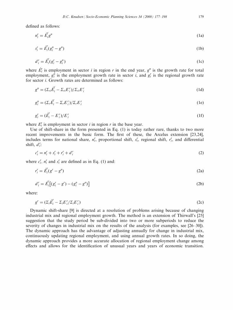
de®ned as follows:

nri � �Er

i gn �1a�

sri � �Er

i �gni ÿ gn� �1b�

d ri � �E

r

i �gri ÿ gni � �1c�where EÂri is employment in sector i in region r in the end year, gn is the growth rate for totalemployment, gni is the employment growth rate in sector i, and gri is the regional growth ratefor sector i. Growth rates are determined as follows:

gn � �Sri�Er

i ÿ SriEri �=SriE

ri �1d�

gni � �Sr�Er

i ÿ SrEri �=SrE

ri �1e�

gri � � �Er

i ÿ E ri �=E r

i �1f�where Er

i is employment in sector i in region r in the base year.Use of shift-share in the form presented in Eq. (1) is today rather rare, thanks to two more

recent improvements in the basic form. The ®rst of these, the Arcelus extension [23,24],includes terms for national share, nri , proportional shift, s

ri , regional shift, r

ri , and di�erential

shift, d ri :

cri � nri � sri � rri � d ri �2�

where cri , nri and sri are de®ned as in Eq. (1) and:

rri � �Er

i �gr ÿ gn� �2a�

d ri � �E

r

i

��gri ÿ gr� ÿ �gni ÿ gn�� 2b�where:

gr � �Si�Er

i ÿ SiEri=SiE

ri � �2c�

Dynamic shift-share [9] is directed at a resolution of problems arising because of changingindustrial mix and regional employment growth. The method is an extension of Thirwall's [25]suggestion that the study period be sub-divided into two or more subperiods to reduce theseverity of changes in industrial mix on the results of the analysis (for examples, see [26±30]).The dynamic approach has the advantage of adjusting annually for change in industrial mix,continuously updating regional employment, and using annual growth rates. In so doing, thedynamic approach provides a more accurate allocation of regional employment change amonge�ects and allows for the identi®cation of unusual years and years of economic transition.

D.C. Knudsen / Socio-Economic Planning Sciences 34 (2000) 177±198 179

Dynamic shift-share provides a solution to the problem of changing industrial mix as well as acorrect estimate of national versus regional growth. To produce a dynamic model, Eqs. (1) or(2) can be computed for all adjacent years. The researcher may then present average annualchange or sum annual change to obtain total national share, sectoral share, and regional shareacross the study period:

Skcrik � Skn

rik � Sks

rik � Skd

rik �3�

where k = 1, . . . ,T is a sequence of adjacent years. The summation can be for a period of anylength.

3. ANOVA-based shift-share models

Berzeg [30] provides a statistical basis for shift-share in terms of Analysis of Variance(ANOVA). In particular, he shows that the shift-share identity can be formalized as the linearmodel:

gri � a� Bi � eri �4�where the national growth rate, gn, is estimated as the model's intercept, a, Bi is an estimate of( gniÿgn ), and error term eri provides an estimate of ( griÿgni ). Assuming a normal distributionfor the eri , the ratio of the parameters to their standard errors will be distributed as Student's tand traditional measures of goodness-of-®t are appropriate.ANOVA-based shift-share is easily adapted to either the Arcelus extension or to the dynamic

context. A probabilistic model of the Arcelus extension has the form (compare [31]):

gri � a� Bi � Gr � eri �5�where terms are de®ned as in Eq. (4), but where Gr=( grÿgn ) and

eri � �gr ÿ gn� ÿ �gni ÿ gn�:As before, assuming a normal distribution for the eri , the ratio of the parameters to theirstandard errors will be distributed as Student's t and traditional measures of goodness-of-®tare appropriate.Adaptation of the model to the dynamic context might include the simple application of

models Eqs. (4) or (5) to each of a succession of years. Alternatively, a dynamic model mightinvolve the addition of another dimension to the analysis, i.e.,

gri � a� Bi � Gr � Vk � eri : �6�In the static case, a=gn, Bi=gniÿgn and eri=griÿgni . In Eq. (6), a=Skg

nk/k, Bi=Sk ( g

nikÿgnk )/k

and erik=Sk ( grikÿgni )/k where k denotes the number of pairs of adjacent years.


4. The relationship between traditional and ANOVA shift-share

The analytical relationship between the various forms of the shift-share model will bediscussed using models (1) and (4), while a more complex comparison will be undertakenempirically. Models (1) and (4) represent the same formulation, the simplest of all shift-sharemodels. Yet, while models (1) and (4) are mathematically equivalent, model (4) when calibratedwill not produce parameters that are identical to those provided by (1) for two reasons. First,Eq. (4) is valued in terms of growth rates while Eq. (1) is valued in terms of employment.Thus, terms in Eqs. (1) and (4) will di�er by Er

i . Second, in Eq. (4), terms eri areheteroscedastic; hence, a is not precisely gn and Bi is not precisely gnÿgni . Berzeg [31,32] showsthat proper choice of weights and use of weighted least squares will yield identical estimates inEqs. (1) and (4). In particular, identical estimates are obtained if it is assumed thatE[er2i ]=(wr

i )ÿ1s 2 instead of the usual assumption that E[er2i ]=s 2 where wr

i=Eri/SriE

ri . Berzeg's

method and an alternative calibration procedure devised by Patterson [33] are compared in theAppendix to this paper. Berzeg's method is shown to be more accurate and lesscomputationally expensive than that proposed by Patterson.The empirical comparison of traditional and ANOVA-based shift-share utilizes data

compiled by the Bureau of Labor Statistics (BLS) of the US Department of Labor for 1939±90as part of their Establishment Survey of Employment, Hours, and Earnings. The data includeentries by BLS industry division and ®ve digit Standard Industrial Code (SIC) for all US statesand possessions. Data on annual employment are comprised of averages of monthly datasurveyed on the twelfth day of each month [34]. Here, these data are aggregated sectorally intothe 9 BLS divisions and spatially into the nine Census divisions.Results of the empirical comparison of models (1) and (4) appear in Table 1. Years 1970 and

1980 are used in this simple comparison. Values in column 1 of the table are generated by thetraditional shift-share model (1). Column 2 of the table presents results for model (4). A

Table 1Comparison of results from simple models

Parameter Model (1) Model (4)

Intercept 0.4721 0.2117Mining 0.0393 0.2997Construction 0.3118 0.5722

Durable manufacturing 0.4905 0.7509Nondurable manufacturing 0.2896 0.5500Transportation and public utilities ÿ0.0241 0.2363Wholesale and retail trade ÿ0.0283 0.2321

F.I.R.E. 0.0735 0.3339Services ÿ0.0646 0.1958Government ÿ0.2604 Aliaseda

R 2 N.A. 0.1836

a Aliased parameters cannot be determined due to insu�cient degrees of freedom.


scatterplot (Fig. 1) of model residuals indicates conformity to the assumption of a normaldistribution.Model (4) is a statistical model, not an accounting model; hence, degrees of freedom must be

considered. Shift-share, from a statistical perspective, is tabular having m rows (sectors) butonly mÿ 1 degrees of freedom. As a result, the parameter associated with one sector cannot beestimated while the remaining parameters are determined only up to an additive constant. Thevalues for proportional shift in Eq. (1) and the parameters obtained for Eq. (4) are thus relatedin the following way. The intercept of Eq. (4) equals the national share component of Eq. (1)plus the proportional shift component associated with government employment, the variable inEq. (4) which cannot be estimated. From Table 1, 0.2117ÿ(ÿ0.2604)=0.2117+0.2604=0.4721.In the same way, the remaining parameters in Eq. (4) equal the corresponding proportionalshift components in Eq. (1) minus the proportional shift component for governmentemployment. It is also evident from the table that the model provides a poor explanation ofthe changes in US employment patterns over the study period. Despite this, some informationcan be gleaned from model (4). The proportional shift parameters associated with construction,durable manufacturing, and nondurable manufacturing are signi®cantly di�erent from theproportional shift parameter associated with government employment (whose parameter is zeroby de®nition).Results of the empirical comparison of the Arcelus extended models (2) and (5) appear in

Table 2. A scatterplot of model (5) residuals (Fig. 2) again demonstrated the reasonableness of

Fig. 1. Standardized residual plot for model (4).


the assumption of a normal distribution. Values in column 1 of the table are generated by thetraditional accounting-based model (2). Column 2 of the table presents results for model (5).In this instance, the parameter associated with one sector and one region cannot be

estimated and the remaining parameters are determined only up to an additive constant. Theintercept of Eq. (5) should therefore equal the national share component of Eq. (2) plus theproportional shift component associated with government employment and the region shiftparameter associated with the Paci®c region Ð the two parameters in Eq. (5) that cannot beestimated. The remaining proportional parameters in Eq. (5) should equal the correspondingproportional shift component in Eq. (2) minus the proportional shift component forgovernment employment, while the remaining regional shift parameters in Eq. (5) should equalthe corresponding regional shift parameters in Eq. (2) minus the regional shift parameterassociated with the Paci®c region.However, this is not the case and some deviation exists between models (2) and (5). In model

(5), for example, goodness-of-®t is improved over that of model (4). Only the proportionalshift parameter for durable manufacturing is signi®cantly di�erent from the proportional shiftparameter of government employment (whose parameter is zero by de®nition).Results of the empirical comparison of dynamic models (3) and (6) appear in Table 3.

Values in column 1 of the table are generated by the conventional shift-share model (3).Column 2 of the table presents results for model (6). Again, the parameter associated with onesector and one region cannot be estimated and the remaining parameters are determined only

Table 2Comparison of results from Arcelus extended models


Intercept 0.4721 0.4184

Mining 0.0393 0.2306Construction 0.3118 0.5308Durable manufacturing 0.4905 0.6572

Nondurable manufacturing 0.2896 0.4703Transportation and public utilities ÿ0.0241 0.1132Wholesale and retail trade ÿ0.0283 0.0952

F.I.R.E. 0.0735 0.3372Services ÿ0.0646 0.1324Government ÿ0.2604 Aliaseda

New England ÿ0.0851 ÿ0.2175Middle Atlantic 0.0149 ÿ0.1459South Atlantic ÿ0.2325 ÿ0.3101East South Central 0.1387 ÿ0.0237East North Central 0.2206 ÿ0.0577West North Central 0.0579 ÿ0.2512West South Central ÿ0.1780 ÿ0.2842Mountain 0.2069 0.0837Paci®c 0.1051 Aliaseda

R 2 N.A. 0.2284



up to an additive constant. Although poor model ®t makes interpretation extremelyproblematic, there again appears to be considerable deviation in the results generated bymodels (3) and (6). However, if the parameter values of government employment and thePaci®c region are subtracted from the intercept of Eq. (6), the resulting value is a closeapproximation of the national share e�ect in Eq. (3). Experimentation shows that the bulk ofvariation in these models is vested in the temporal parameter (Vk in Eq. (6)) and that thedynamic shift-share strategy proposed by Bar� and Knight [9] is the best way of capturing this.

5. Information-theoretic shift-share models

Previous use and methodological innovation in the realm of shift-share has taken placewithin the traditional accounting and ANOVA-based techniques. A principal di�erencebetween the bulk of previous research on shift-share and the research reported here is areliance on information-theoretic methods. In order to illustrate the e�cacy of these methods,it is necessary to illustrate two things. First, that information-theoretic methods lead to modelsthat are at least as diverse as the those obtained under the traditional accounting-based andANOVA-based formats. Second, it must be shown that they are superior performers based onstandard goodness-of-®t measures.Shift-share analyses based on information theory rely on the information gain measure of

Fig. 2. Standardized residual plot for model (5).


Kullback and Leibler [35]:

I�P:Q� � Sripri ln� pri=qri � �7�

where, qri represents an element of a prior probability distribution and pri represents an elementof a posterior probability distribution. The measure I(P:Q) thus measures the informationgained from observing distribution P given distribution Q. Within the context of shift-shareanalysis, pri=EÂri/SriEÂ

ri and qri=Er

i/SriEri . Construction of a variety of shift-share models is

possible by considering the general problem:

min I�P:Q� � Sripri ln� pri=qri � pri �8�

subject to:

1: Sripri f

t�xrti � � xt; for all t

2: SSripri � 1

3: prie0; for all i and j

where ft(xrti ) represents some function in t of observed values xri and xt represents some

Table 3Comparison of results from dynamic models


Intercept 1.2446 0.6367

Mining ÿ0.3853 0.1334Construction ÿ0.1685 0.0751Durable manufacturing ÿ0.0205 0.3176

Nondurable manufacturing ÿ0.3403 0.0863Transportation and public utilities ÿ0.5246 ÿ0.0763Wholesale and retail trade ÿ0.3083 0.2189

F.I.R.E. 0.1980 0.0946Services 0.6107 0.3520Government 0.0998 Aliaseda

New England 0.5689 0.6244

Middle Atlantic 1.0037 0.8224South Atlantic 1.4318 0.8535East South Central 0.3811 0.6742

East North Central ÿ0.2255 0.4096West North Central ÿ0.5601 0.0654West South Central ÿ0.8353 ÿ0.1981Mountain ÿ0.7044 ÿ0.0322Paci®c ÿ0.6945 Aliaseda

R 2 N.A. 0.0111



exogenously speci®ed limiting value. Direct solution of Eq. (8) is possible, but it is moreconvenient to solve the dual of Eq. (8) which is an unconstrained geometric programmingproblem [36,37]:

max F�lt� � Sriqri exp

�Stl

tf t�xrti �� Stl

txt � l0 �9�

where lt and l 0 are unconstrained dual variables [38]. This approach to the solution of Eq. (9)is not generally employed in planning, regional science and geography. Rather, planners,regional scientists and geographers tend to exploit two other properties of Eqs. (8) and (9).First, when the constraints in Eq. (8) are linear equalities, programs (8) and (9) lead directly

to a model of quantities pri from the application of Lagrangian methods:

ln pri � ln qri ÿ l0 ÿ Stltf t�xrt

i �: �10�Second, quantities pri , l

t, and l 0 that result from the solution of Eqs. (8), (9) or (10) areasymptotic maximum likelihood estimators [39]. As a result, planners, regional scientists andgeographers tend to estimate model (10) using maximum likelihood methods [40,41]. Use of themaximum likelihood approach ensures asymptotic normality of the model parameters [42].This, in turn, simpli®es hypothesis testing and assessment of goodness-of-®t. The ratio ofparameters to their standard errors is asymptotically normal and goodness-of-®t is measured asdeviance which is asymptotic chi-square distributed.Information gain has been used to derive both shift-share measures of spatial concentration

[43,44] and shift-share models based on minimum discrimination information (MDI) [45±49].To arrive at the information-based model proposed by Theil and Gosh [45], ®rst form theMDI primal:

min I�P:Q� � Sripri ln� pri=qri � �11�

subject to:

1: Srpri � oi; for all i

2: prie0; for all r and i

where oi is the frequency of employment in sector i and other terms are as previously de®ned.In this case, application of Lagrangian methods results in the model:

pri � qri exp�a� oi � � f ri : �12�

This model can in turn be rewritten as the dynamic model [50]:

�Er

i � E ri exp�A� Oi � � F r

i �13�

where Oi is total employment in industry i, A is the intercept and Fri is the error term. Suitable

rearrangement yields:


ln� �Er

i=Eri � � A� Oi � ln�F r

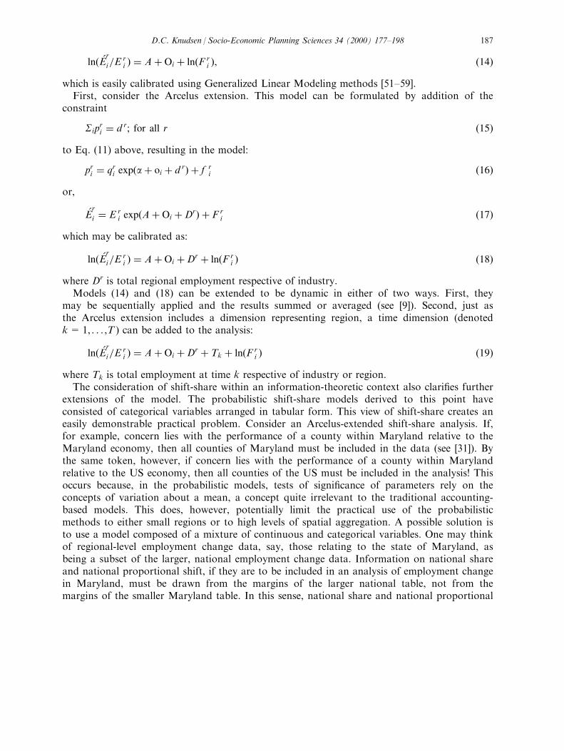
i �, �14�which is easily calibrated using Generalized Linear Modeling methods [51±59].First, consider the Arcelus extension. This model can be formulated by addition of the

constraint

Sipri � d r; for all r �15�

to Eq. (11) above, resulting in the model:

pri � qri exp�a� oi � d r� � f ri �16�

or,

�Er

i � E ri exp�A� Oi �Dr� � F r

i �17�which may be calibrated as:

ln� �Er

i=Eri � � A� Oi �Dr � ln�F r

i � �18�where Dr is total regional employment respective of industry.Models (14) and (18) can be extended to be dynamic in either of two ways. First, they

may be sequentially applied and the results summed or averaged (see [9]). Second, just asthe Arcelus extension includes a dimension representing region, a time dimension (denotedk=1, . . . ,T ) can be added to the analysis:

ln� �Er

i=Eri � � A� Oi �Dr � Tk � ln�F r

i � �19�where Tk is total employment at time k respective of industry or region.The consideration of shift-share within an information-theoretic context also clari®es further

extensions of the model. The probabilistic shift-share models derived to this point haveconsisted of categorical variables arranged in tabular form. This view of shift-share creates aneasily demonstrable practical problem. Consider an Arcelus-extended shift-share analysis. If,for example, concern lies with the performance of a county within Maryland relative to theMaryland economy, then all counties of Maryland must be included in the data (see [31]). Bythe same token, however, if concern lies with the performance of a county within Marylandrelative to the US economy, then all counties of the US must be included in the analysis! Thisoccurs because, in the probabilistic models, tests of signi®cance of parameters rely on theconcepts of variation about a mean, a concept quite irrelevant to the traditional accounting-based models. This does, however, potentially limit the practical use of the probabilisticmethods to either small regions or to high levels of spatial aggregation. A possible solution isto use a model composed of a mixture of continuous and categorical variables. One may thinkof regional-level employment change data, say, those relating to the state of Maryland, asbeing a subset of the larger, national employment change data. Information on national shareand national proportional shift, if they are to be included in an analysis of employment changein Maryland, must be drawn from the margins of the larger national table, not from themargins of the smaller Maryland table. In this sense, national share and national proportional


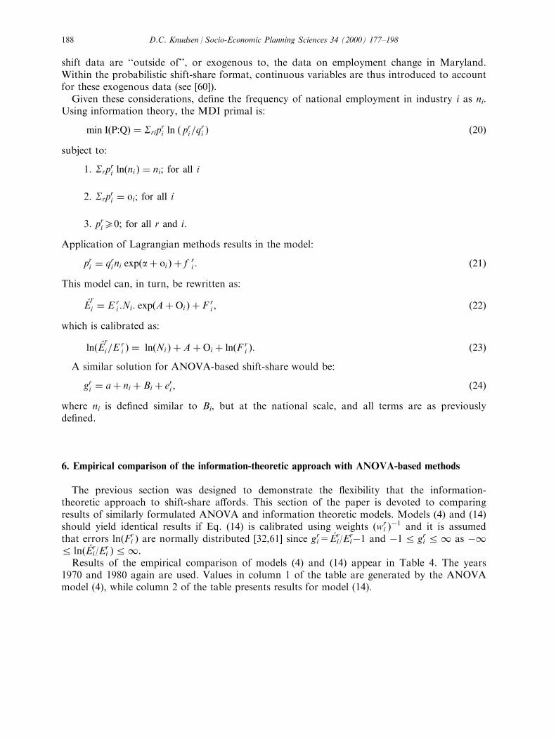
shift data are ``outside of'', or exogenous to, the data on employment change in Maryland.Within the probabilistic shift-share format, continuous variables are thus introduced to accountfor these exogenous data (see [60]).Given these considerations, de®ne the frequency of national employment in industry i as ni.

Using information theory, the MDI primal is:

min I�P:Q� � Sripri ln � pri=qri � �20�

subject to:

1: Srpri ln�ni � � ni; for all i

2: Srpri � oi; for all i

3: prie0; for all r and i:

Application of Lagrangian methods results in the model:

pri � qri ni exp�a� oi � � f ri : �21�

This model can, in turn, be rewritten as:

�Er

i � E ri :Ni: exp�A� Oi � � F r

i , �22�which is calibrated as:

ln� �Er

i=Eri � � ln�Ni � � A� Oi � ln�F r

i �: �23�A similar solution for ANOVA-based shift-share would be:

gri � a� ni � Bi � eri , �24�where ni is de®ned similar to Bi, but at the national scale, and all terms are as previouslyde®ned.

6. Empirical comparison of the information-theoretic approach with ANOVA-based methods

The previous section was designed to demonstrate the ¯exibility that the information-theoretic approach to shift-share a�ords. This section of the paper is devoted to comparingresults of similarly formulated ANOVA and information theoretic models. Models (4) and (14)should yield identical results if Eq. (14) is calibrated using weights (wr

i )ÿ1 and it is assumed

that errors ln(Fri ) are normally distributed [32,61] since gri=EÂri/E

riÿ1 and ÿ1 R gri R1 as ÿ1

R ln(EÂri/Eri )R1.

Results of the empirical comparison of models (4) and (14) appear in Table 4. The years1970 and 1980 again are used. Values in column 1 of the table are generated by the ANOVAmodel (4), while column 2 of the table presents results for model (14).


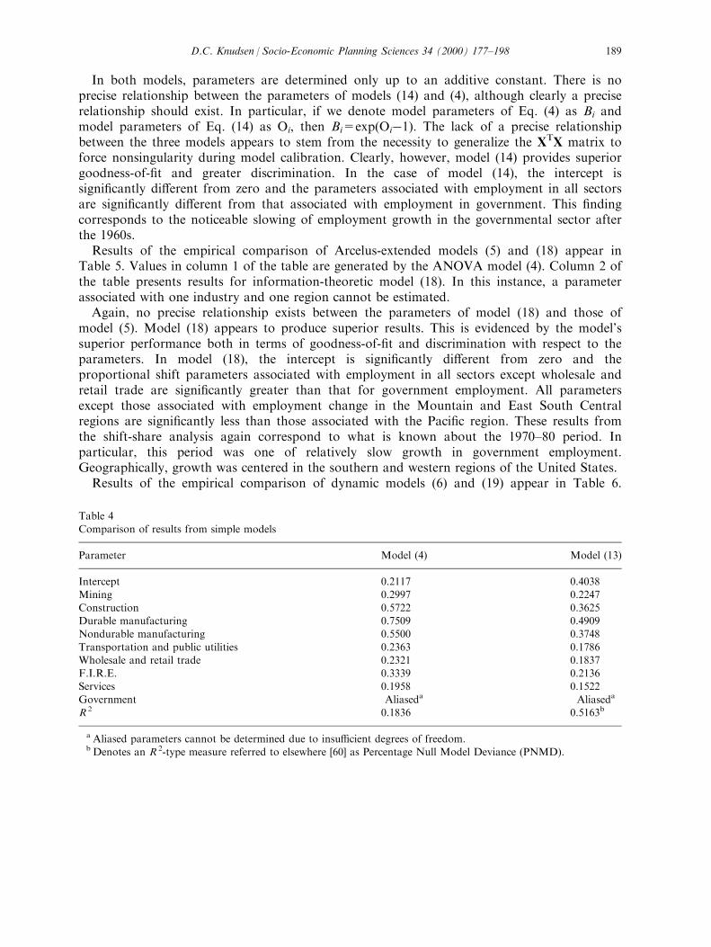
In both models, parameters are determined only up to an additive constant. There is noprecise relationship between the parameters of models (14) and (4), although clearly a preciserelationship should exist. In particular, if we denote model parameters of Eq. (4) as Bi andmodel parameters of Eq. (14) as Oi, then Bi=exp(Oiÿ1). The lack of a precise relationshipbetween the three models appears to stem from the necessity to generalize the XTX matrix toforce nonsingularity during model calibration. Clearly, however, model (14) provides superiorgoodness-of-®t and greater discrimination. In the case of model (14), the intercept issigni®cantly di�erent from zero and the parameters associated with employment in all sectorsare signi®cantly di�erent from that associated with employment in government. This ®ndingcorresponds to the noticeable slowing of employment growth in the governmental sector afterthe 1960s.Results of the empirical comparison of Arcelus-extended models (5) and (18) appear in

Table 5. Values in column 1 of the table are generated by the ANOVA model (4). Column 2 ofthe table presents results for information-theoretic model (18). In this instance, a parameterassociated with one industry and one region cannot be estimated.Again, no precise relationship exists between the parameters of model (18) and those of

model (5). Model (18) appears to produce superior results. This is evidenced by the model'ssuperior performance both in terms of goodness-of-®t and discrimination with respect to theparameters. In model (18), the intercept is signi®cantly di�erent from zero and theproportional shift parameters associated with employment in all sectors except wholesale andretail trade are signi®cantly greater than that for government employment. All parametersexcept those associated with employment change in the Mountain and East South Centralregions are signi®cantly less than those associated with the Paci®c region. These results fromthe shift-share analysis again correspond to what is known about the 1970±80 period. Inparticular, this period was one of relatively slow growth in government employment.Geographically, growth was centered in the southern and western regions of the United States.Results of the empirical comparison of dynamic models (6) and (19) appear in Table 6.

Table 4

Comparison of results from simple models


Intercept 0.2117 0.4038Mining 0.2997 0.2247

Construction 0.5722 0.3625Durable manufacturing 0.7509 0.4909Nondurable manufacturing 0.5500 0.3748

Transportation and public utilities 0.2363 0.1786Wholesale and retail trade 0.2321 0.1837F.I.R.E. 0.3339 0.2136Services 0.1958 0.1522

Government Aliaseda Aliaseda

R 2 0.1836 0.5163b

a Aliased parameters cannot be determined due to insu�cient degrees of freedom.b Denotes an R 2-type measure referred to elsewhere [60] as Percentage Null Model Deviance (PNMD).


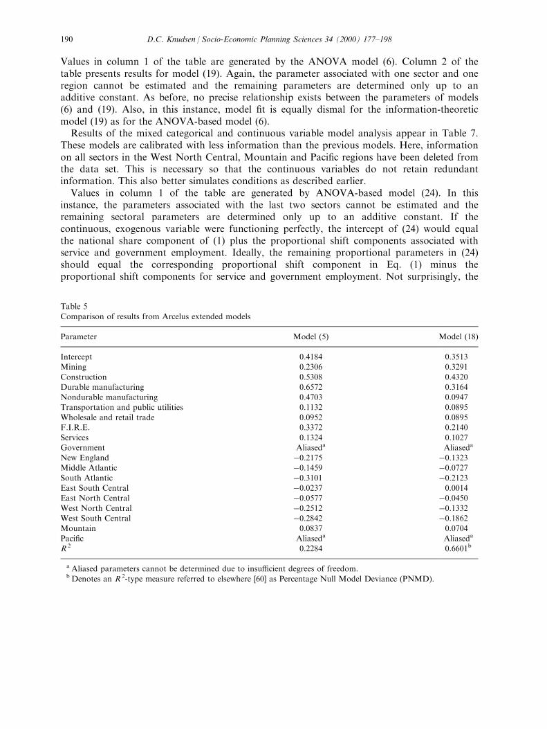
Values in column 1 of the table are generated by the ANOVA model (6). Column 2 of thetable presents results for model (19). Again, the parameter associated with one sector and oneregion cannot be estimated and the remaining parameters are determined only up to anadditive constant. As before, no precise relationship exists between the parameters of models(6) and (19). Also, in this instance, model ®t is equally dismal for the information-theoreticmodel (19) as for the ANOVA-based model (6).Results of the mixed categorical and continuous variable model analysis appear in Table 7.

These models are calibrated with less information than the previous models. Here, informationon all sectors in the West North Central, Mountain and Paci®c regions have been deleted fromthe data set. This is necessary so that the continuous variables do not retain redundantinformation. This also better simulates conditions as described earlier.Values in column 1 of the table are generated by ANOVA-based model (24). In this

instance, the parameters associated with the last two sectors cannot be estimated and theremaining sectoral parameters are determined only up to an additive constant. If thecontinuous, exogenous variable were functioning perfectly, the intercept of (24) would equalthe national share component of (1) plus the proportional shift components associated withservice and government employment. Ideally, the remaining proportional parameters in (24)should equal the corresponding proportional shift component in Eq. (1) minus theproportional shift components for service and government employment. Not surprisingly, the



Intercept 0.4184 0.3513Mining 0.2306 0.3291

Construction 0.5308 0.4320Durable manufacturing 0.6572 0.3164Nondurable manufacturing 0.4703 0.0947

Transportation and public utilities 0.1132 0.0895Wholesale and retail trade 0.0952 0.0895F.I.R.E. 0.3372 0.2140

Services 0.1324 0.1027Government Aliaseda Aliaseda

New England ÿ0.2175 ÿ0.1323Middle Atlantic ÿ0.1459 ÿ0.0727South Atlantic ÿ0.3101 ÿ0.2123East South Central ÿ0.0237 0.0014East North Central ÿ0.0577 ÿ0.0450West North Central ÿ0.2512 ÿ0.1332West South Central ÿ0.2842 ÿ0.1862Mountain 0.0837 0.0704

Paci®c Aliaseda Aliaseda

R 2 0.2284 0.6601b



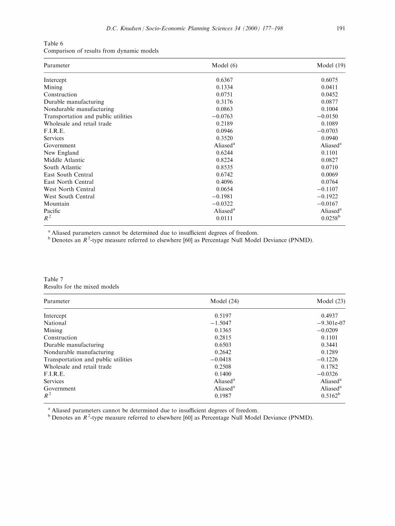
Table 6Comparison of results from dynamic models


Intercept 0.6367 0.6075Mining 0.1334 0.0411Construction 0.0751 0.0452

Durable manufacturing 0.3176 0.0877Nondurable manufacturing 0.0863 0.1004Transportation and public utilities ÿ0.0763 ÿ0.0150Wholesale and retail trade 0.2189 0.1089F.I.R.E. 0.0946 ÿ0.0703Services 0.3520 0.0940Government Aliaseda Aliaseda

New England 0.6244 0.1101Middle Atlantic 0.8224 0.0827South Atlantic 0.8535 0.0710

East South Central 0.6742 0.0069East North Central 0.4096 0.0764West North Central 0.0654 ÿ0.1107West South Central ÿ0.1981 ÿ0.1922Mountain ÿ0.0322 ÿ0.0167Paci®c Aliaseda Aliaseda

R 2 0.0111 0.0258b


Table 7Results for the mixed models


Intercept 0.5197 0.4937National ÿ1.5047 ÿ9.301e-07Mining 0.1365 ÿ0.0209Construction 0.2815 0.1101Durable manufacturing 0.6503 0.3441

Nondurable manufacturing 0.2642 0.1289Transportation and public utilities ÿ0.0418 ÿ0.1226Wholesale and retail trade 0.2508 0.1782F.I.R.E. 0.1400 ÿ0.0326Services Aliaseda Aliaseda

Government Aliaseda Aliaseda

R 2 0.1987 0.5162b



exogenous variable is not functioning perfectly; hence, this is not the case. Rather, somedeviation exists between models (1) and (24). However, model goodness-of-®t of Eq. (24)exceeds that of Eq. (1). This is unexpected since, theoretically, Eq. (24) is calibrated using lessinformation than is the case for Eq. (1). This may be an artifact of the poor ®t of model (1).Only the parameter associated with durable manufacturing signi®cantly exceeds thoseassociated with service and government employment (whose parameters are zero by de®nition).Column 2 of the table presents results for model (23). If the continuous, exogenous variable

were functioning perfectly, models (23) and (13) would produce identical results. As was thecase for the ANOVA-based model, the exogenous variable is not functioning perfectly.Further, model goodness-of-®t of Eq. (13) exceeds that of Eq. (23). Since Eq. (23) is calibratedusing less information, this is entirely expected. The parameters associated with durablemanufacturing and wholesale and retail trade signi®cantly exceed those associated with serviceand government employment (again, whose parameters are zero by de®nition).

7. Conclusions and implications of the research

Shift-share is a relatively old ex-post analysis technique that measures the ends of the processof change rather than the variables that are the agents of change. The technique additionallyhas been criticized because of its assumptions concerning the linearity of regional economicdynamics and its lack of ability to handle regional variation.These objections, while containing some truth, ignore three realities. First, recent

improvements such as the Arcelus extension and dynamic shift-share have lessened thetechnique's reliance on the assumed long-term linearity of regional dynamics. In so doing, theyhave created models much more able to measure regional variation. Indeed, the thrust of thispaper has been to illustrate that probabilistic forms of shift-share models (and, particularly,information theory-based models) are members of a highly ¯exible class of variance-partitioning methods, akin to the family of spatial interaction models delineated by Wilson[41]. This implies that shift-share is but one example of the broader class of models used in theanalysis of aggregate tabular data within planning, geography and regional science. Moregenerally, probabilistic shift-share provides a major advance over traditional accounting-basedmethods because it allows the researcher to quantitatively test hypotheses about changes inemployment or value added by region or sector [61].Second, the construction of causal models of regional economic development presupposes

that, as researchers, we have a clearly de®ned theory of regional economic development. Thiswould appear not to be the case. The last decade has been a period of extreme tumult amongboth regional economic development theoreticians and regional economies. While variance-partitioning models, such as shift-share, do not explain economic phenomenon, they do allowus to allocate variation among competing alternatives (national sectoral shift versus regionalshift, independent of sector), and thus bring us closer to explanation.Also, probabilistic shift-share has a number of implications for the validation of theories in

geography and regional science that are best demonstrated by example. Consider the ongoingdebate on the relative importance of the global economy versus the local economy indetermining employment patterns (classics include [62,63]). Shift-share models contain two


components, national share and proportional shift, that might be termed ``global'', and anotherterm, di�erential shift, that might be termed ``local'' in that it approximates, somewhat crudely,regional or local uniqueness. Suppose that models such as Eqs. (1), (4), and (14) are employedin the analysis of employment trends and it is found that model ®t is poor. A reasonableconclusion might be that regional or local uniqueness, not global restructuring, lies at the heartof changing employment patterns.Third, within the context of economic policy implementation, policy-makers are frequently

overwhelmed by the sheer volume of information available. There exists, therefore, a need forquick, inexpensive analysis tools that are neither mathematically complex nor data intensive.Shift-share analysis is one such tool. Probabilistic shift-share provides a sound statistical basisfor shift-share analysis. Since policy outcomes are, in part, dependent on the quality ofinformation available, improving the quality of tools through which policy-makers ®lterinformation should lead to improved policy [63±66].While the results presented here must be treated with caution, there also appears to be

support for further use of information-theoretic models in the analysis of shift-sharerelationships. In this regard, such models have three positive characteristics. First, they providea ¯exible vehicle for the derivation of shift-share models. Second, casting shift-share ininformation-theoretic terms places the methodology squarely into the mainstream statisticalanalysis of nominal, tabular data. Additionally, information-theoretic models have propertiesthat are particularly useful for the analysis of selected forms of data. The information-theoreticform used here appears to be especially useful for analyzing data characterized by a smallnumber of relatively large outliers. This issue is treated more fully by Flowerdew and Aitkin[53]. These advantages, however, must be weighed against the more di�cult interpretation ofinformation-theoretic models when used to analyze shift-share (see previous discussion and[67]).

Acknowledgements

The author would like to thank without implicating Stephen Deppen and Mark Fitch forhelp with the computational aspects of this research and the anonymous referees whosecomments substantially improved the paper. This paper is based upon work supported by theNational Science Foundation under Grant No. SES-9022747.

Appendix A

A1. Alternative calibration of the ANOVA shift-share model

An alternative calibration of the ANOVA shift-share model was devised by Patterson [33].Patterson calibrates Eq. (4) subject to constraints that ensure that SiuiBi=0 for all i where ui isthe national employment in sector i. Should model (5) be used, then it must be the case thatSiuiBi=0 for all i and Sjv

jGj=0 for all j where vj is regional employment in j across allindustries. This necessitates the use of constrained regression [68]. The resulting models are:


g ji � a� Bi � e j

i �4a�subject to:

SiuiBi � 0 for all i

and

g ji � a� Bi � G j � e j

i �5a�subject to:

SiuiBi � 0 for all i

SjvjG j � 0 for all j

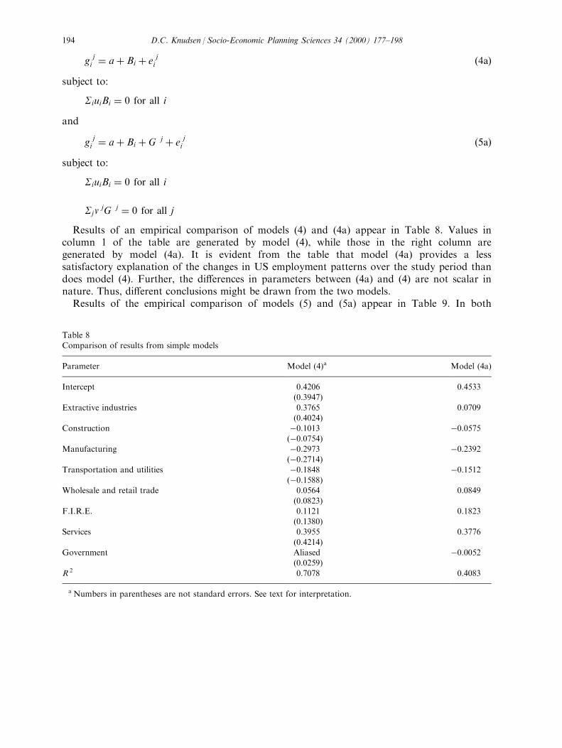
Results of an empirical comparison of models (4) and (4a) appear in Table 8. Values incolumn 1 of the table are generated by model (4), while those in the right column aregenerated by model (4a). It is evident from the table that model (4a) provides a lesssatisfactory explanation of the changes in US employment patterns over the study period thandoes model (4). Further, the di�erences in parameters between (4a) and (4) are not scalar innature. Thus, di�erent conclusions might be drawn from the two models.Results of the empirical comparison of models (5) and (5a) appear in Table 9. In both

Table 8Comparison of results from simple models

Parameter Model (4)a Model (4a)

Intercept 0.4206 0.4533

(0.3947)Extractive industries 0.3765 0.0709

(0.4024)Construction ÿ0.1013 ÿ0.0575

(ÿ0.0754)Manufacturing ÿ0.2973 ÿ0.2392

(ÿ0.2714)Transportation and utilities ÿ0.1848 ÿ0.1512

(ÿ0.1588)Wholesale and retail trade 0.0564 0.0849

(0.0823)F.I.R.E. 0.1121 0.1823

(0.1380)Services 0.3955 0.3776

(0.4214)Government Aliased ÿ0.0052

(0.0259)

R 2 0.7078 0.4083

a Numbers in parentheses are not standard errors. See text for interpretation.


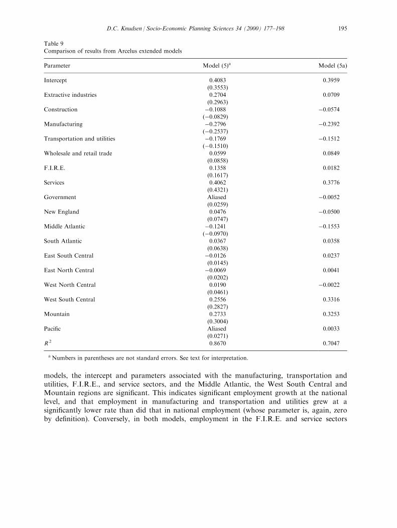
models, the intercept and parameters associated with the manufacturing, transportation andutilities, F.I.R.E., and service sectors, and the Middle Atlantic, the West South Central andMountain regions are signi®cant. This indicates signi®cant employment growth at the nationallevel, and that employment in manufacturing and transportation and utilities grew at asigni®cantly lower rate than did that in national employment (whose parameter is, again, zeroby de®nition). Conversely, in both models, employment in the F.I.R.E. and service sectors


Parameter Model (5)a Model (5a)

Intercept 0.4083 0.3959(0.3553)

Extractive industries 0.2704 0.0709

(0.2963)Construction ÿ0.1088 ÿ0.0574

(ÿ0.0829)Manufacturing ÿ0.2796 ÿ0.2392

(ÿ0.2537)Transportation and utilities ÿ0.1769 ÿ0.1512

(ÿ0.1510)Wholesale and retail trade 0.0599 0.0849

(0.0858)F.I.R.E. 0.1358 0.0182

(0.1617)Services 0.4062 0.3776

(0.4321)

Government Aliased ÿ0.0052(0.0259)

New England 0.0476 ÿ0.0500(0.0747)

Middle Atlantic ÿ0.1241 ÿ0.1553(ÿ0.0970)

South Atlantic 0.0367 0.0358

(0.0638)East South Central ÿ0.0126 0.0237

(0.0145)

East North Central ÿ0.0069 0.0041(0.0202)

West North Central 0.0190 ÿ0.0022(0.0461)

West South Central 0.2556 0.3316(0.2827)

Mountain 0.2733 0.3253

(0.3004)Paci®c Aliased 0.0033

(0.0271)

R 2 0.8670 0.7047

a Numbers in parentheses are not standard errors. See text for interpretation.


grew signi®cantly faster than did national employment. Regionally, employment in the MiddleAtlantic region grew at a signi®cantly lower rate, while the West South Central and Mountainregions grew at a signi®cantly greater rate than did the nation as a whole. However, as was thecase for model (4), in model (5) the lower R 2 associated with model (5a) indicates that themodel provides a slightly less satisfactory explanation of the changes in US employmentpatterns over the study period than does model (5).Summarizing, while the results presented here must be treated with caution, there appears to

be some support for suggesting that Berzeg's calibration method [31,32] is superior to thatproposed by Patterson. Perhaps the most noticeable characteristic of Berzeg's approach is itssuperior explanatory power. On the other hand, it is worth noting that the two modelsmeasure slightly di�erent things. Berzeg's formulation measures growth in relation to abaseline industry and region, while Patterson's formulation measures growth with respect tonational averages. Patterson's formulation is the more conventional and is more consistentwhen extended to the Arcelus form, but this, we feel, does not justify its use given that it is lessaccurate and computationally more expensive.

References

[1] Glickman NJ, Glasmeier A. The international economy and the American South. In: Rodwin L, Sazanami H,editors. Deindustrialization and regional transformation: the experience of the United States. Boston: UnwinHyman, 1989. p. 60±80.

[2] Harrison B, Kluver J. Reassessing the Massachusetts miracle. Environment and Planning A 1989;21:771±801.[3] Markusen AR, Carlson V. Deindustrialization in the American Midwest: causes and responses. In: Rodwin L,

Sazanami H, editors. Deindustrialization and regional transformation: the experience of the United States.

Boston: Unwin Hyman, 1989. p. 29±59.[4] Hu� D, Sherr L. Measure for determining di�erential growth rates of markets. Journal of Market Geography

1967;4:391±5.

[5] Plane DA. The geographic components of change in a migration system. Geographical Analysis 1987;19:283±99.

[6] Plane DA, Rogerson P. U.S. migration pattern responses to the oil glut and recession of the early 1980s: anapplication of shift-share and causative matrix techniques. In: Congdon P, Batey P, editors. Advances in

regional demography. London: Belhaven Press, 1989. p. 386±414.[7] Bar� RA, Knight III PL. The role of federal military spending in the timing of the New England employment

turnaround. Papers of the Regional Science Association 1988;65:151±66.

[8] Casler SD. A theoretical context for shift and share analysis. Regional Studies 1989;23:43±8.[9] Bar� RA, Knight III PL. Dynamic shift-share analysis. Growth and Change 1988;19:1±10.[10] Houston DB. The shift and share analysis of regional growth: a critique. Southern Economic Journal

1967;33:577±81.[11] Richardson HW. The state of regional economics: a survey article. International Regional Science Review

1978;3:1±48.[12] Buck TW. Shift-share analysis: a guide to regional policy? Regional Studies 1970;4:445±50.

[13] Holden DR, Swales JK, Nairn AGM. The repeated application of shift-share: a structural explanation ofregional growth? Environment and Planning A 1987;19:1233±50.

[14] Stillwell FJB. Further thoughts on the shift and share approach. Regional Studies 1970;4:451±8.

[15] Hellman DA. Shift-share models as predictive tools. Growth and Change 1976;7:3±8.[16] Kurre JA, Weller BR. Forecasting the local economy, using time-series and shift-share techniques. Environment

and Planning A 1989;21:753±70.


[17] Stevens BH, Moore CL. A critical review of the shift-share as a forecasting technique. Journal of Regional

Science 1980;20:419±37.

[18] Rigby DL, Anderson WP. Employment change, growth and productivity in Canadian manufacturing: an

extension and application of shift-share analysis. Canadian Journal of Regional Science/Revue Canadienne des

Sciences Regionales 1993;26:69±88.

[19] Haynes KE, Dinc M. Productivity change in manufacturing regions: a multifactor/shift-share approach.

Growth and Change 1997;28:150±70.

[20] Creamer DB. Industrial location and natural resources. Washington, DC: US Natural Resources Planning

Board, 1943.

[21] Dunn Jr ES. A statistical and analytical technique for regional analysis. Papers of the Regional Science

Association 1960;6:97±112.

[22] Perlo� HS, et al. Regions, resources and economic growth. Baltimore: Johns Hopkins University Press, 1960.

[23] Arcelus FJ. An extension of shift-share analysis. Growth and Change 1984;15:3±8.

[24] Esteban-Marquillas JM. Shift- and share-analysis revisited. Regional and Urban Economics 1972;2:249±61.

[25] Thirlwall AP. A measure of the proper distribution of industry. Oxford Economic Papers 1967;19:46±58.

[26] Brown HJ. Shift-share projections of regional growth: An empirical test. Journal of Regional Science 1969;9:1±

18.

[27] Browne LE. The impact of industry mix on New England's economic growth since 1950. New England

Economic Indicators 1977;April:33.

[28] Fothergill S, Gudgin G. In defense of shift-share. Urban Studies 1979;16:309±19.

[29] Jackson G, et al. Regional diversity: growth in the United States, 1960±1990. Boston: Auburn House, 1981.

[30] Lever WF. The inner-city employment problem in Great Britian, 1952±76: a shift-share approach. In: Rees J, et

al., editors. Industrial location and regional systems. New York: Bergin, 1981.

[31] Berzeg K. The empirical content of shift-share analysis. Journal of Regional Science 1978;18:463±9.

[32] Berzeg K. A note on statistical approaches to shift-share analysis. Journal of Regional Science 1984;24:277±85.

[33] Patterson M. A note on the formulation of a full-analogue regression model of the shift-share method. Journal

of Regional Science 1991;31:211±6.

[34] Bureau of Labor Statistics. Establishment survey of employment, hours, and earnings. Washington, DC: US

Government Printing O�ce, n.d.

[35] Kullback S, Leibler RA. On information and su�ciency. Annals of Mathematical Statistics 1951;22:78±86.

[36] Brockett PL, Charnes A, Cooper WW. M.D.I. Estimation via unconstrained convex programming. Austin, TX:

Center for Cybernetic Studies, 1978.

[37] Knudsen DC. Exploring ¯ow system change: U.S. rail freight ¯ows, 1972±1981. Annals of the Association of

American Geographers 1985;75:539±51.

[38] Fiacco AV, McCormick GP. Nonlinear programming: sequential unconstrained minimization techniques. New

York: Wiley, 1968.

[39] Phillips FY. A guide to MDI statistics for planning and management model-building. Austin: Institute for

Constructive Capitalism, 1981.

[40] Williams PA, Fotheringham AS. The calibration of spatial interaction models by maximum likelihood

estimation with program SIMODEL. Bloomington, IN: Indiana University, Department of Geography

(Geographic Monograph Series), 1984.

[41] Wilson AG. Entropy in urban and regional modelling. London: Pion, 1970.

[42] Feinberg SE. Analysis of cross-classi®ed data. Cambridge, MA: MIT Press, 1981.

[43] Haynes KE, Machunda ZB. Considerations in extending shift-share analysis. Growth and Change 1987;18:69±

78.

[44] Haynes KE, Machunda ZB. Decomposition of change in spatial employment concentration: an information-

theoretic extension of shift-share analysis. Papers of the Regional Science Association 1988;65:101±13.

[45] Theil H, Gosh R. A comparison of shift-share and the RAS adjustment. Regional Science and Urban

Economics 1980;10:175±80.

[46] Berry BJL, Schwind PJ. Information and entropy in migrant ¯ows. Geographical Analysis 1969;1:5±14.

[47] Haynes KE, Phillips FY. Constrained minimum discrimination information: a unifying tool for modeling

spatial and individual choice behavior. Environment and Planning A 1982;14:1341±54.


[48] Kullback S. Information and statistics. New York: Wiley, 1959.[49] Thomas RW. Information statistics in geography. Norwich: GeoAbstracts, 1981.

[50] Knudsen DC. Generalizing Poisson regression: including a priori information using the method of o�sets. TheProfessional Geographer 1992;44:202±8.

[51] Baxter M. Similarities in methods of estimating spatial interaction models. Geographical Analysis 1982;14:267±

72.[52] Baxter M. A note on the estimation of a nonlinear migration model using GLIM. Geographical Analysis

1984;16:282±6.

[53] Flowerdew R, Aitkin M. A method of ®tting the gravity model based on the Poisson distribution. Journal ofRegional Science 1982;22:191±202.

[54] Flowerdew R, Lovett A. Fitting constrained Poisson regression models to interurban migration ¯ows.

Geographical Analysis 1988;20:297±307.[55] Flowerdew R, Lovett A. Compound and generalized Poisson models for interurban migration. In: Congdon P,

Batey P, editors. Advances in regional demography. London: Belhaven Press, 1989. p. 246±56.[56] Gokhale DV, Kullback S. The information in contingency tables. New York: Marcel Dekker, 1978.

[57] Lovett A, Flowerdew R. Analysis of count data using Poisson regression. Professional Geographer1989;41:190±8.

[58] Lovett A, Whyte ID, Whyte KA. Poisson regression analysis and migration ®elds: the example of the

apprenticeship records of Edinburgh in the seventeenth and eighteenth centuries. Transactions of the Instituteof British Geographers, New Series 1985;10:317±32.

[59] McCullagh P, Nelder JA. Generalized linear models. London: Chapman & Hall, 1983.

[60] Knudsen DC. Manufacturing employment change in the American Midwest, 1977±86. Environment andPlanning A 1992;24:1303±16.

[61] Knudsen DC, Bar� R. Shift-share as a linear model. Environment and Planning A 1991;23:421±31.

[62] Massey DB, Meegan R. The anatomy of job loss: the how, why, and where of employment decline. London:Methuen, London, 1982.

[63] Murgatroyd L, Urry J. The class and gender restructuring of the Lancaster economy, 1950±1980. In: Localities,class and gender. London: The Lancaster Regionalism Group, Pion, 1985. p. 30±53.

[64] Brewer GD, deLeon P. The foundations of policy analysis. Homewood, IL: Dorsey Press, 1983.[65] Laswell HD. A preview of policy sciences. New York: Elsevier, 1971.[66] Weimer DL, Vining AR. Policy analysis: concepts and practice. Englewood Cli�s, NJ: Prentice Hall, 1989.

[67] Theil H, Sorooshian C. Components of the change in regional inequality. Economics Letters 1979;4:191±3.[68] Pringle RM, Raynor AA. Generalised inverse matrices with applications to statistics. New York: Hafner, 1971.


shift-share analysis: further examination of models for ...directory.umm.ac.id/data...

Documents