shiva newsletter #5 februaryshiva.iup.uni-heidelberg.de/dl/shiva_newsletter_no5_feb2012.pdf · very...

SHIVA Newsletter #5 February 2012


The 5th SHIVA newsletter reports on the activities performed within the EU project SHIVA (Stratospheric ozone: Halogen Impacts in a Varying Atmosphere, grant number 226224) during the second half of 2011. The core activity during the last 6 months was the successful western Pacific campaign in Malaysia from Sept. to Dec. 2011. A short summary is presented in WP‐2. More details can be found on the SHIVA web (http://shiva.iup.uni‐heidelberg.de/news.html) and Wiki page. Furthermore, we want to express our gratitude to all the people, especially our Malaysian partners, who made the SHIVA campaign possible and a success.

Thanks to all work package leaders and contributors to this newsletter.

With our bests regards,

Marcel Dorf and Klaus Pfeilsticker

Report on activities within the individual Work Packages (WPs)

WP‐1: Management

Meetings: Summaries, minutes and presentations can be found on the Wiki

• The annual meeting 2011 and a half‐day campaign planning meeting took place in Leeds on July 14/15.

• September 7: Meeting in Kuala Lumpur with Malaysian scientist for planning the deployment of small boats during the SHIVA campaign.

• September 8/9: Steering Committee and campaign preparation meeting in Kuala Lumpur.

Administration:

• Amendment No.2 to the Consortium Agreement was signed by all participants – necessary due to the change in aircraft for the campaign (HALO had to be replaced by FALCON in the document).

• Press releases were issued before and after the campaign by UHEI, DLR, IFM‐GEOMAR and UM

• A campaign report was compiled and post‐campaign reporting to the Malaysian authorities was done in Kuala Lumpur.

• A 12 month extension of the SHIVA project till June 2013 was initiated.

1


Reminder:

• The data protocol has to be signed by all campaign participants. You can download it from the Wiki. Please also remind newly hired students to sign it.

• Proper acknowledgement (using SHIVA‐226224‐FP7‐ENV‐2008‐1) to the European Commission must be given in all SHIVA publications or publications using any SHIVA data.

• Please upload missing campaign information to the SHIVA wiki‐page (http://shiva.iup.uni‐heidelberg.de/wiki/).

WP‐2: Measurements

The major achievement of the past 6 months has been the SHIVA field campaign in the western Pacific, which ran from early November to mid December 2011. The major components of the campaign were:

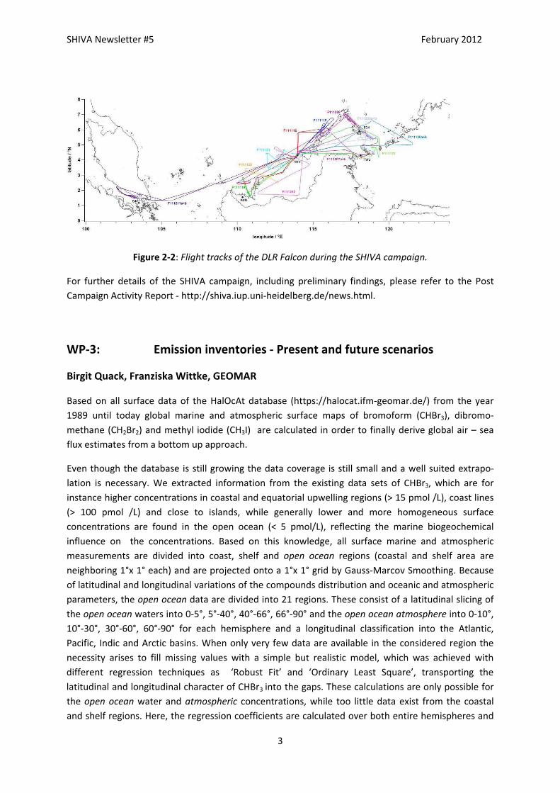
1. A cruise of the RV Sonne from Singapore to the Philippines (Figure 2‐1) 2. The deployment of the DLR Falcon aircraft from a base in Miri, Sarawak (Figure 2‐2) 3. A ground‐based campaign on Bohey Dulang island (Sabah) 4. Three local 1‐day boat expeditions 5. Laboratory and coastal measurements of VSLS source strenghts

The various measurement activities were supported by extensive meteorological analysis, satellite‐retrievals and modelling activity.

Figure 2‐1: Track of the RV Sonne from Singapore (15/11/11) to the Philippines (29/11/11). 2

http://shiva.iup.uni-heidelberg.de/wiki/

http://shiva.iup.uni-heidelberg.de/wiki/


Figure 2‐2: Flight tracks of the DLR Falcon during the SHIVA campaign.

For further details of the SHIVA campaign, including preliminary findings, please refer to the Post Campaign Activity Report ‐ http://shiva.iup.uni‐heidelberg.de/news.html.

WP‐3: Emission inventories ‐ Present and future scenarios

Birgit Quack, Franziska Wittke, GEOMAR

Based on all surface data of the HalOcAt database (https://halocat.ifm‐geomar.de/) from the year 1989 until today global marine and atmospheric surface maps of bromoform (CHBr3), dibromo‐methane (CH2Br2) and methyl iodide (CH3I) are calculated in order to finally derive global air – sea flux estimates from a bottom up approach.

Even though the database is still growing the data coverage is still small and a well suited extrapo‐lation is necessary. We extracted information from the existing data sets of CHBr3, which are for instance higher concentrations in coastal and equatorial upwelling regions (> 15 pmol /L), coast lines (> 100 pmol /L) and close to islands, while generally lower and more homogeneous surface concentrations are found in the open ocean (< 5 pmol/L), reflecting the marine biogeochemical influence on the concentrations. Based on this knowledge, all surface marine and atmospheric measurements are divided into coast, shelf and open ocean regions (coastal and shelf area are neighboring 1°x 1° each) and are projected onto a 1°x 1° grid by Gauss‐Marcov Smoothing. Because of latitudinal and longitudinal variations of the compounds distribution and oceanic and atmospheric parameters, the open ocean data are divided into 21 regions. These consist of a latitudinal slicing of the open ocean waters into 0‐5°, 5°‐40°, 40°‐66°, 66°‐90° and the open ocean atmosphere into 0‐10°, 10°‐30°, 30°‐60°, 60°‐90° for each hemisphere and a longitudinal classification into the Atlantic, Pacific, Indic and Arctic basins. When only very few data are available in the considered region the necessity arises to fill missing values with a simple but realistic model, which was achieved with different regression techniques as ‘Robust Fit’ and ‘Ordinary Least Square’, transporting the latitudinal and longitudinal character of CHBr3 into the gaps. These calculations are only possible for the open ocean water and atmospheric concentrations, while too little data exist from the coastal and shelf regions. Here, the regression coefficients are calculated over both entire hemispheres and

3


are only depending on latitude. The idea of the biogeochemical division of ocean and atmosphere is transferred for CH2Br2 and CH3I, which are treated and extrapolated in a similar way. The developed surface concentration climatology for ocean and atmosphere are used for global air‐sea flux calculations for each considered halocarbon compound. Compared to recent studies, negative fluxes are located in each climatology, which mainly occur in the Arctic and Antarctic region. We estimate positive global fluxes for CHBr3, CH2Br2, and CH3I of respectively 210 to 326, 88 to 105 gG Br yr‐1 and 182 to 216 gG I yr‐1 and negative fluxes of ‐66 to ‐74, ‐30.4 to ‐26 gG Br yr‐1 and ‐0.9 to ‐1.0 gG I yr‐1. A publication about these air‐sea flux calculations is currently in preparation by Wittke et al., while the data have already been provided to some modeling groups within SHIVA.

As outlook we aim at improving the existing parameterization for bromoform in the next months, while we currently evaluate the obscure correlations between bromoform and biological, physical and chemical parameters of individual cruises and the global data set. We then strive after the calculation of future air – sea fluxes for all three regarded compounds in order to estimate the strength of variation in a changing environment. Quality control and enlargement of the HalOcAt database is continued.

WP‐4: Process studies ‐ Transport and pathways

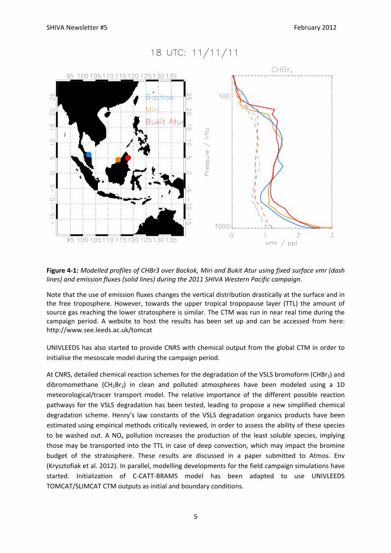
UNIVLEEDS have continued to investigate the troposphere‐stratosphere transport and chemistry of very short‐lived species (VSLS) using the TOMCAT/SLIMCAT 3‐D chemical transport model (CTM). For bromoform (CHBr3) and dibromomethane (CH2Br2), the model now uses the spatially‐varying, but temporally fixed, emission estimates of Liang et al. (2010). Previously a uniform prescribed mixing ratio was imposed in the surface level of the model (~1.2 ppt for each source gas). This simple approach showed the CTM could reproduce some features of observed vertical profiles of these gases in the tropics. However, model profiles of CHBr3 lacked a distinct "c‐shape" as has been observed and is likely a signature of convection. These comparisons have been made for a range of aircraft campaigns (Hossaini et al., 2010; 2012). Use of emission fluxes should now allow the CTM to capture more variability at the surface and may indeed produce "hot spots" where the abundance of CHBr3 and CH2Br2 is relatively large. These regions may coexist with regions of strong convective upwelling (e.g., Western Pacific). Thus use of emissions fluxes will likely also change the modelled vertical distribution of VSLS. This is shown in Figure 4‐1.

4


Figure 4‐1: Modelled profiles of CHBr3 over Backok, Miri and Bukit Atur using fixed surface vmr (dash lines) and emission fluxes (solid lines) during the 2011 SHIVA Western Pacific campaign.

Note that the use of emission fluxes changes the vertical distribution drastically at the surface and in the free troposphere. However, towards the upper tropical tropopause layer (TTL) the amount of source gas reaching the lower stratosphere is similar. The CTM was run in near real time during the campaign period. A website to host the results has been set up and can be accessed from here: http://www.see.leeds.ac.uk/tomcat UNIVLEEDS has also started to provide CNRS with chemical output from the global CTM in order to initialise the mesoscale model during the campaign period.

At CNRS, detailed chemical reaction schemes for the degradation of the VSLS bromoform (CHBr3) and dibromomethane (CH2Br2) in clean and polluted atmospheres have been modeled using a 1D meteorological/tracer transport model. The relative importance of the different possible reaction pathways for the VSLS degradation has been tested, leading to propose a new simplified chemical degradation scheme. Henry’s law constants of the VSLS degradation organics products have been estimated using empirical methods critically reviewed, in order to assess the ability of these species to be washed out. A NOx pollution increases the production of the least soluble species, implying those may be transported into the TTL in case of deep convection, which may impact the bromine budget of the stratosphere. These results are discussed in a paper submitted to Atmos. Env (Krysztofiak et al. 2012). In parallel, modelling developments for the field campaign simulations have started. Initialization of C‐CATT‐BRAMS model has been adapted to use UNIVLEEDS TOMCAT/SLIMCAT CTM outputs as initial and boundary conditions.

5

http://www.see.leeds.ac.uk/tomcat


UNIHB has performed CTM time slice experiments of Arctic winter ozone depletion of the SCIAMACHY/ENVISAT period 2002 to 2011. Special emphasis was given to assess the severe Arctic ozone losses which were observed in winter‐spring 2011. Several changes were made on the model configuration, which lead to an overall good agreement between modelled and observed total ozone (GOME‐2) and the vertical distributions of O3, NO2 and BrO from SCIAMACHY limb. It has been shown that small differences in model description of atmospheric heating rates may cause large overestimations of northern hemispheric total ozone. This also has an effect on the modelled abundance of lower stratospheric bromine, predominantly in mid‐latitudes and the tropics. A re‐examination of modelled stratospheric bromine has been started and concentrate on the ENSO modulated upwelling of short and long‐lived brominated substances in the upper troposphere/lower stratosphere.

UNIHB also continued the screening of the SCIAMACHY/ENVISAT limb data product of bromine monoxide in the stratosphere. A new retrieval version was introduced implying a correction of the measured spectra with respect to the pointing misalignment of the instrument, which affects in particular the quality of the data product in the first years of measurement from August 2002 ‐ 2004. Thereby, orbital mean pointing corrections from TRUE algorithm were applied to each particular limb measurement. The correction was made only for tropical measurements where the maximum pointing uncertainty is expected from the previous studies. The effect of this correction on the inferred long‐term trend of stratospheric BrO is found to be 0.2% above 17 km altitude, and 0.5% below.

References

Hossaini, R., Chipperfield, M. P., Feng, W., Breider, T. J., Atlas, E., Montzka, S. A., Miller, B. R., Moore, F., and Elkins, J.: The contribution of natural and anthropogenic very short‐lived species to stratospheric bromine, Atmos. Chem. Phys., 12, 371‐380, 2012.

Krysztofiak, G., V. Catoire, G. Poulet, V. Marécal, M. Pirre, F. Louis, S. Canneaux, B. Josse, Detailed modeling of the atmospheric degradation mechanism of brominated very‐short lived species, submitted to Atmospheric Environment, 2012.

Marécal, V., Pirre, M., Krysztofiak, G., and Josse, B.: What do we learn on bromoform transport and chemistry in deep convection from fine scale modelling?, Atmos. Chem. Phys. Discuss, 11, 29561‐29600, 2011.

Sinnhuber, B.‐M., G. Stiller, R. Ruhnke, T. von Clarmann, S. Kellmann, and J. Aschmann (2011), Arctic winter 2010/2011 at the brink of an ozone hole, Geophys. Res. Lett., 38, L24814, doi:10.1029/2011GL049784.

WP‐5: Stratospheric halogens ‐ Analysis of measured trends and projections

UNIHB further investigated time series and long‐term trends of SCIAMACHY/ENVISAT limb retrieved bromine monoxide (plus nitrogen dioxide and ozone) profiles in the stratosphere. Since it was shown in earlier work that the estimated trends of SCIAMACHY limb observed BrO might be affected by a drift in the pointing misalignment of the instrument, UNIHB introduced a correction of this error

6


based on the TRUE algorithm (von Savigny et al., 2005). While in previous estimations monthly mean BrO profiles were linearly corrected based on the monthly mean pointing offsets, the new retrieval version applies orbital mean corrections directly to measured spectra before the retrieval. The investigations show that for high latitudes, the pointing error is negligible, while in the tropics it affects the estimated long‐term trend of stratospheric BrO in the order of 0.2% per year between the 17 and 26 km altitude, and by 0.5% per year at altitudes below.

BIRA has updated the trend analysis of stratospheric bromine from collocated SCIAMACHY limb (version 3.2 of the IUP‐Bremen scientific product) and ground‐based UV‐visible observations at the Harestua (60°N, 11°E) and OHP (44°N, 5.5°E) stations till April 2011. Regarding the ground‐based measurements at Harestua, the DOAS analysis has been improved through the use of the 342‐359 nm wavelength range, a Taylor expansion of the ozone optical depth (Pukite et al., 2010), and the O4 cross sections from Greenblatt et al. (1990). It allows including data from campaigns held in 1994‐1996 and therefore covering the 1994‐2011 period in the trend analysis. These settings will be also applied in the future to measurements at OHP. As previously reported, a positive trend of about +2.5%/year is inferred before 2001 at both stations from ground‐based UV‐visible observations, while a negative trend of about ‐1%/year is found since 2001 in SCIAMACHY limb and ground‐based data sets. A trend analysis has been also performed on ground‐based data sets using a statistical model including appropriate geophysical forcings (solar flux, QBO, and evolution of the bromine sources). This analysis further confirms that the trend of stratospheric BrO is mainly driven by the evolution of the sources.

Relying on the good stability of the SCIAMACHY nadir total BrO column dataset (BIRA scientific product), a long‐term trend analysis has been initiated. The analysis exploits the data at high solar zenith angles (>80°; in the polar region) – for which we have a high sensitivity to the stratosphere. Preliminary results show a decreasing trend of ‐1 %/year of the BrO column over the 2002‐2011 period, in agreement with the above estimates obtained from ground‐based and SCIAMACHY limb BrO observations. The next step is to further consolidate these results and to extend the trend analysis to the GOME‐SCIAMACHY merged data set covering the 1996‐2011 period.

The work on the tropical bromine budget by GUF, announced in the report for the first 6 months of 2011, is now accepted for publication in Atmospheric Chemistry and Physics (Brinkmann et al., 2012). GUF has further performed measurements for brominated source gases during the SHIVA Falcon aircraft campaign in Miri (see WP 2). These are the first in‐situ GC‐MS observations of a wide suite of short lived halogenated compounds, including all important bromine VSLS and CH3I. As a further contribution to WP 5, Andreas Engel (project PI from GUF) has accepted the invitation to serve as a lead author for a SPARC assessment report on lifetimes of halogenated hydrocarbons. The first draft of this report is to be finished by late April 2012 and this is expected to make an important contribution to improving the understanding of the stratospheric halogen budget.

7


References

Brinkmann, S. et al., Short‐lived brominated species – Observations in the source regions and the tropical tropopause layer, Atmos. Chem. Phys., in press, 2012.

Greenblatt, G. D., et al., Absorption measurements of oxygen between 330 and 1140 nm, J. Geophys. Res., 95, 18557‐18582, 1990

Pukite, J., et al., Extending differential optical absorption spectroscopy for limb measurements in the UV, Atmos. Meas. Tech., 3, 631‐653, 2010

von Savigny, C. and Kaiser, J.W. and Bovensmann, H. and Burrows, J.P. and McDermid, I.S. and Leblanc, T. (2005) Spatial and temporal Characterization of SCIAMACHY Limb Pointing Errors during the first three Years of the Mission. Atmos. Chem. Phys., 5 . pp. 2593‐2602.

WP‐6: Global modeling of VSLS, for the past, present and future

WP Leader: UCAM (S. Fueglistaler) Groups: U Leeds (M. Chipperfield, R. Hossaini) U Cambridge (J. Pyle, J. Yang) IFM (K. Krüger, S. Tegtmeier) AWI (M. Rex, I. Wohltmann)

Summary: For WP‐6, no milestones and deliverables were scheduled for this period. No problems or delays were reported.

U Cambridge: During the past 6 months, UCAM has finished adding the photochemical kinetics data (e.g. absorption cross sections and quantum yields) for newly introduced photolysis reactions in the UKCA chemistry scheme such that the model can do online Fast‐Jx calculation. Numerical model calculations to explore the lifetime of various Cl‐containing and Br‐containing species in the stratosphere are now running. A scheme for bromine heterogeneous reactions on Polar Stratospheric Clouds and stratospheric aerosols has been implemented in the model. Further analysis and validation of the modelled stratospheric halogen species (Cl, Br) as well as ozone are currently being undertaken. In addition, we are in the final stages of setting up the model to investigate the effect of VSLS on stratospheric ozone ina future climate (i.e. ~2100).

U Leeds: The University of Leeds (UNIVLEEDS) have continued to investigate the troposphere‐stratosphere transport and chemistry of very short‐lived species (VSLS) using the TOMCAT/SLIMCAT 3‐D chemical transport model (CTM). The model has been used to quantify the contribution of VSLS to the inorganic bromine (Bry) budget of the stratosphere. Previous estimates of BryVSLS by UNIVLEEDS have considered the major VSLS bromoform (CHBr3) and dibromomethane (CH2Br2) only (Hossaini et al., 2010). The CTM now also contains dibromochloromethane (CHBr2Cl), bromodichloromethane (CHBrCl2), bromochloromethane (CH2BrCl) and ethyl bromide (C2H5Br). Inclusion of these minor VSLS

8


in the CTM leads to a BryVSLS contribution of ~4.9‐5.2 parts per trillion (ppt) ‐ consistent with estimates derived from balloon‐borne measurements of BrO (e.g., Dorf et al., 2008). These results indicate that CHBr3 and CH2Br2 account for ~76% of BryVSLS and that VSLS accounted for ~25% of total Bry in the lower stratosphere in 2009. Figure 6‐1 shows the total bromine contribution from long‐lived source gases included in the CTM and also VSLS.

CH Br3 H1211 H1301 H2402

CHBr3 CH Br2 2 CHBr Cl2 CHBrCl2

CH BrCl2 C H Br2 5 VSLS ALL

Br / ppt

Pre

ssure

/ h

Pa

1000

100

0.1 1.0 10.0

Figure 6‐2: Modelled total bromine contribution of long‐lived source gases & VSLS. From Hossaini et al. (2012)

Modelled VSLS profiles have been compared with new observations from the 2009 NSF HIPPO‐1 aircraft campaign along with ongoing surface measurements by NOAA/ESRL. Modelled profiles give good agreement with the aircraft observations in the boundary layer and the lower tropical tropopause layer (TTL).

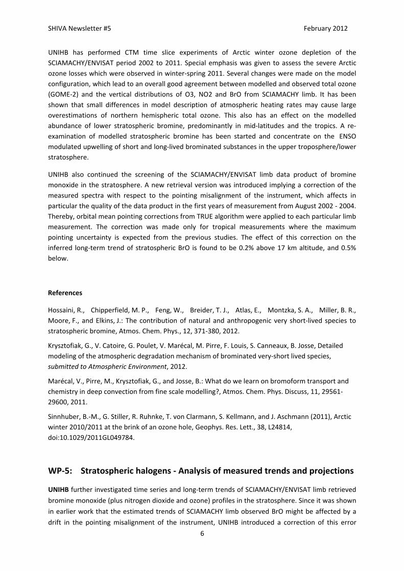
UNIVLEEDS have also examined the local photochemical lifetime of 4 VSLS of anthropogenic origin; ethyl bromide (C2H5Br), ethylene dibromide (CH2BrCH2Br), n‐propyl bromide (n‐C3H7Br) and i‐propyl bromide (i‐C3H7Br). Figure 6‐2 shows the lifetime with respect to oxidation with OH, photolysis and also the overall local lifetime of these gases in the tropics. For C2H5Br and, in particular CH2BrCH2Br, the local lifetime in the cold TTL may be long (> 6 months) and thus outside of the World Meteorological Organisation (WMO) working definition of a VSLS. These gases are potentially important carriers of bromine to the stratosphere. However at present their emissions are small.

9


10

OH

LocalA B

C D

Pre

ssure

/ h

Pa

Lifetime / days Lifetime / days

Lifetime / days Lifetime / days

Pre

ssure

/ h

Pa

10

1000

100

10

1

1000

100

10

1

1000

100

10

1

1000

100

10

1

0 50 100 150 200 0 500 1000 1500

0 20 40 60 0 20 40 60

hν

Figure 6‐3: Local lifetime of anthropogenic VSLS in the tropics. From Hossaini et al. (2012)

UNIVLEEDS have also begun to use the UKCA chemistry‐climate model (CCM) to investigate the impact of BryVSLS on present day and future stratospheric ozone. Preliminary results and comparisons with aircraft data suggest UKCA simulates the vertical distribution of VSLS CHBr3 and CH2Br2 extremely well in the TTL and lower stratosphere. The model will be used to examine potential transport changes under future projected climates and the impact on the delivery of BryVSLS to the stratosphere.

References

Hossaini, R., Chipperfield, M. P., Feng, W., Breider, T. J., Atlas, E., Montzka, S. A., Miller, B. R., Moore, F., and Elkins, J.: The contribution of natural and anthropogenic very short‐lived species to stratospheric bromine, Atmos. Chem. Phys., 12, 371‐380, 2012.

Hossaini, R., Chipperfield, M. P., Monge‐Sanz, B. M., Richards, N. A. D., Atlas, E., and Blake, D. R.: Bromoform and dibromomethane in the tropics: a 3‐D model study of chemistry and transport, Atmos. Chem. Phys., 10, 719‐735, doi:10.5194/acp‐10‐719‐2010, 2010.

Tegtmeier, S., K. Krüger, B. Quack, I. Pisso, A. Stohl, and X. Yang, Bridging the gap between halocarbon oceanic emissions and upper air concentrations, to be submitted.

shiva newsletter #5 februaryshiva.iup.uni-heidelberg.de/dl/shiva_newsletter_no5_feb2012.pdf · very...

Documents