shock analysis of an antenna structure subjected to
TRANSCRIPT

SHOCK ANALYSIS OF AN ANTENNA STRUCTURE SUBJECTED TO
UNDERWATER EXPLOSIONS
A THESIS SUBMITTED TO
THE GRADUATE SCHOOL OF NATURAL AND APPLIED SCIENCES
OF
MIDDLE EAST TECHNICAL UNIVERSITY
BY
MEHMET EMRE DEMİR
IN PARTIAL FULFILLMENT OF THE REQUIREMENTS
FOR
THE DEGREE OF MASTER OF SCIENCE
IN
MECHANICAL ENGINEERING
SEPTEMBER 2015


Approval of the thesis:
SHOCK ANALYSIS OF AN ANTENNA STRUCTURE SUBJECTED TO
UNDERWATER EXPLOSIONS
submitted by MEHMET EMRE DEMİR in partial fulfillment of the requirements
for the degree of Master of Science in Mechanical Engineering Department,
Middle East Technical University by,
Prof. Dr. Gülbin Dural Ünver
Dean, Graduate School of Natural and Applied Sciences _________________
Prof. Dr. Tuna Balkan
Head of Department, Mechanical Engineering _________________
Prof. Dr. Mehmet Çalışkan
Supervisor, Mechanical Engineering Dept., METU _________________
Examining Committee Members:
Prof. Dr. R. Orhan Yıldırım
Mechanical Engineering Department, METU _________________
Prof. Dr. Mehmet Çalışkan
Mechanical Engineering Department, METU _________________
Assoc. Prof. Dr. Yiğit Yazıcıoğlu
Mechanical Engineering Department, METU _________________
Asst. Prof. Dr. Gökhan O. Özgen
Mechanical Engineering Department, METU _________________
Asst. Prof. Dr. Bülent İrfanoğlu
Mechatronics Engineering Department, Atılım University _________________
Date: 08.09.2015

iv
I hereby declare that all information in this document has been obtained and
presented in accordance with academic rules and ethical conduct. I also
declare that, as required by these rules and conduct, I have fully cited and
referenced all material and results that are not original to this work.
Name, Last name: Mehmet Emre DEMİR
Signature:

v
ABSTRACT
SHOCK ANALYSIS OF AN ANTENNA STRUCTURE SUBJECTED TO
UNDERWATER EXPLOSIONS
Demir, Mehmet Emre
M. S., Department of Mechanical Engineering
Supervisor: Prof. Dr. Mehmet Çalışkan
September 2015, 183 pages
Antenna structures constitute main parts of electronic warfare systems. Mechanical
design is as crucial as electromagnetic design of antenna structures for proper
functioning and meeting high system performance needs. Failure of mechanical
and electronic structures operating under shock loading is a common occurrence in
naval electronic warfare applications. A complete shock analysis of the dipole
antenna structure subjected to underwater explosions is performed to foresee
adverse effects of mechanical shock phenomena on the antenna structure.
Theoretical models of the antenna structure; namely mathematical model and finite
element model, are built on multi-degree-of-freedom approach. Modal properties
are derived from Classical Beam Theory and transient responses to input shock
loading are obtained by Recursive Filtering Relationship (RFR) Method for the
mathematical model. Input shock loading is synthesized from assessed shock
specification to classical shock input. Transient responses exerted from RFR
method are also approximated by simplified and SDOF models. Finite element
analysis of the analytical model is performed on ANSYS® platform. Comparisons
of analytical results are presented for interchangeable use of proposed models.

vi
Numerical results are verified with both modal and transient results collected from
experimental analysis. Experimental analysis is performed for exact dimensions of
antenna structure subjected to synthesized shock input criteria.
Shock severity for antenna structure is presented for both electrical and mechanical
components. Design roadmap is drawn within the limitations set for proper antenna
functioning with desired performance. Design limitations are determined by the
verified mathematical model. Shock isolation theory is also explained and applied
to the antenna structure in order to obtain shock responses below limitations
mentioned. Thus, the complete shock analysis of the antenna structure is performed
for antenna design to withstand underwater shock explosions.
Keywords: Underwater Explosions (UNDEX), Shock Profile Synthesis, Transient
Response Analysis, Experimental Shock Analysis, Shock Isolation.

vii
ÖZ
SU ALTI PATLAMARINA MARUZ KALAN BİR ANTEN YAPISININ
ŞOK ANALİZİ
Demir, Mehmet Emre
Yüksek Lisans, Makina Mühendisliği Bölümü
Tez Yöneticisi: Prof. Dr. Mehmet Çalışkan
Eylül 2015, 183 sayfa
Elektronik harp sistemlerinin en önemli parçası anten yapılarıdır. Yüksek sistem
performansı ve sürekli çalışabilen bir anten yapısı elde edebilmek için
elektromanyetik tasarım kadar mekanik tasarım da kritik öneme sahiptir. Deniz
platformunda çalışan elektronik harp sistemleri yüksek şok yüklemeleri altında
çalıştığından, mekanik ve elektronik yapılarda sıklıkla arızalar veya
deformasyonlar gözlenmektedir. Bu etkileri tahmin edilir hale getirebilmek, şoka
dayanıklı tasarımlar ortaya koyabilmek ve tasarım aşamasında gerekli önlemleri
alabilmek için bir dipol antenin şok analizi sunulmuştur.
Anten yapısı, matematiksel metotlar ve sonlu elemanlar metoduyla çok serbestlik
dereceli olarak modellenmiştir. Antenin modal özellikleri Klasik Kiriş Teorisi ile,
şok cevapları da Yinelemeli Filtreleme İlişkisi(YFİ) Metodu ile modellenmiştir.
Antene etki eden şok tahriki, antenin dayanması gereken şok limitlerine göre
sentezlenen klasik dalga profilleriyle verilmiştir. YFİ metoduyla elde edilen şok
tepkilerine, basitleştirilmiş modellerle ve tek serbestlik dereceli modelle de
yaklaşımlarda bulunulmuştur. Analitik modelin sonlu elemanlar analizi ANSYS®
programı ile gerçekleştirilmiştir. Matematiksel model ve sonlu elemanlar analizi
sonuçları kıyaslanarak gerektiğinde birbirlerinin yerine kullanımları

viii
değerlendirilmiştir. Analitik sonuçlar deneysel modal analiz ve deneysel şok analizi
ile doğrulanmıştır. Deneyler bire bir anten modellerine daha önce sentezlenen şok
profilleri uygulanarak gerçekleştirilmiştir.
Antende yer alan elektriksel ve mekanik parçaların şoka karşı dayanımı
sunulmuştur. Antenin çalışmasını ve istenen performansı sağlayabilmesi için
belirlenen tasarım sınırları tasarım yol haritası içerisinde ortaya konmuş ve tasarım
için incelenmesi gereken adımlar belirtilmiştir. Tasarım sınırları belirlenirken
doğrulanmış olan matematiksel model kullanılmıştır. Antenin bu sınırlar içerisinde
mekanik şoktan etkilenmeden çalışabilmesi için şok izolasyonu teorisi ve şok
izolasyonu basamakları sunulmuştur. Çalışmada incelenen anten yapısının şok
izolasyonu gerçekleştirilerek şoktan etkilenmeden çalışabilmesi sağlanmıştır.
Anahtar Kelimeler: Denizaltı Patlamaları, Mekanik Şok, Şok Profil Sentezi, Şok
Tepki Analizi, Deneysel Şok Analizi, Şok İzolasyonu.

ix
To My Family,

x
ACKNOWLEDGEMENTS
I would like to express my sincere gratitude to my advisor, Prof. Dr. Mehmet
Çalışkan, for his guidance, support and technical suggestions throughout the study.
I am grateful to ASELSAN A.Ş. for the financial and technical opportunities
provided for the completion of this thesis.
I would also like to express my sincere appreciation for Yunus Emre Özçelik,
Rahmi Dündar, Emrah Gedikli, Murat Atacan Avgın, Yasin Özdoğan, Caner
Asbaş, Durmuş Gebeşoğlu, Ahmet Dindar, Ahmet Muaz Ateş, Özkan Sağlam and
Merve Öztürk for their valuable friendship, motivation and help.
I would like to thank to Yusuf Başıbüyük for his guidance, help and comments
throughout the drop experiments.
For their understanding my spending lots of time on this work, I sincerely thank to
my family.

xi
TABLE OF CONTENTS
ABSTRACT ........................................................................................................ V
ÖZ ...................................................................................................................... VII
ACKNOWLEDGEMENTS ................................................................................ X
TABLE OF CONTENTS ................................................................................... XI
LIST OF TABLES ........................................................................................... XV
LIST OF FIGURES ........................................................................................ XVII
LIST OF SYMBOLS ....................................................................................... XXI
LIST OF ABBREVIATIONS ...................................................................... XXIII
CHAPTERS
1 INTRODUCTION .............................................................................................. 1
Naval C-ESM/COMINT Antennas ....................................................... 4
Mechanical Shock ................................................................................. 5
Ship Shock and Underwater Explosions (UNDEX) ........................... 12
Motivation ........................................................................................... 13
Scope, Objective and Contribution of Work ....................................... 14
Outline of the Dissertation .................................................................. 16
2 LITERATURE SURVEY ................................................................................. 19
Historical Background......................................................................... 19
Literature Survey ................................................................................. 21
3 SHOCK PROFILE SYNTHESIS ..................................................................... 29
Theory: Shock Response Spectrum..................................................... 29
Shock Response Spectrum for Naval Applications............................. 35
Determination of Assessment Criteria from Shock Response Spectrum
..........................................................................................................................37
Shock Synthesis................................................................................... 40
xii
3.4.1 Longitudinal (X) Axis Shock Synthesis .......................................... 41
3.4.2 Transverse (Y) Axis Shock Synthesis ............................................. 42
3.4.3 Vertical (Z) Axis Shock Synthesis .................................................. 43
4 MATHEMATICAL MODELING OF THE ANTENNA STRUCTURE ......... 45
Problem Definition .......................................................................................... 45
Modal Transient Response of the Antenna Structure Subjected to Base
Excitation......................................................................................................... 47
4.1.1 Normal Modes, Natural Frequencies and Mode Shapes of the
Antenna Structure ........................................................................................ 48
4.1.2 Effective Modal Mass and Participation Factor for the Antenna
Structure ...................................................................................................... 53
4.1.3 Transient Response of the Antenna Structure to Base Excitation ... 54
Solution Methods for Transient Response of the Antenna Structure
Subjected to Base Excitation ........................................................................... 59
4.2.1 Multi-Degree-of-Freedom (MDOF) Solution Methods .................. 61
4.2.1.1 Ramp Invariant Recursive Filtering Relationship Method ...... 61
4.2.1.2 Other Numerical Methods ....................................................... 62
4.2.2 Single-Degree-of-Freedom (SDOF) Solution Methods .................. 63
4.2.2.1 Convolution Integral Method .................................................. 63
4.2.2.2 Digital Recursive Filtering Relationship Method ................... 64
4.2.2.3 Newmark-Beta Method ........................................................... 64
4.2.2.4 Runge-Kutta 4th Order Method ............................................... 65
4.2.3 Simplified Solution Models............................................................. 65
4.2.3.1 Absolute Sum Method (ABSSUM) ......................................... 65
4.2.3.2 Square Root of the Sum of the Squares (SRSS) ...................... 66
4.2.3.3 Naval Research Laboratories Method (NRLM) ...................... 66
5 TRANSIENT RESPONSE ANALYSIS OF ANTENNA STRUCTURE ........ 69
Modal Analysis of Antenna Structure ................................................. 70
MDOF Transient Response Analysis of Antenna Structure ............... 72
5.2.1 Determination of Analysis Parameters ............................................ 72
5.2.2 MDOF Transient Response Analysis Results ................................. 79
xiii
Transient Analysis Results of Antenna Structure by Simplified
Methods ........................................................................................................... 86
5.3.1 Transient Response Results of ABSSUM Method ......................... 87
5.3.2 Transient Response Results of SRSS Method................................. 88
5.3.3 Transient Response Results of NRL Method .................................. 88
Transient Analysis Results of Antenna Structure Using SDOF Models
………………………………………………………………………………..90
Comments of Chapter 5....................................................................... 95
6 TRANSIENT RESPONSE ANALYSIS OF ANTENNA STRUCTURE BY
FINITE ELEMENT ANALYSIS ........................................................................ 97
Modal Analysis of Antenna Structure ................................................. 98
Transient Response Analysis of Antenna Structure .......................... 101
Discussion for Chapter 6 ................................................................... 106
7 EXPERIMENTAL ANALYSIS OF ANTENNA STRUCTURE ................... 109
Introduction ....................................................................................... 109
Modal Verification of Antenna by Impact Hammer Test ................. 110
Drop Experiment of Antenna Structure ............................................ 118
Comments on Verification Results ................................................... 124
8 SHOCK SEVERITY FOR ANTENNA STRUCTURE .................................. 127
Shock Effects on Antenna Performance............................................ 127
Shock Severity Limits for Electrical Components on Antenna
Structure ........................................................................................................ 131
Shock Stress Severity on Antenna Structure ..................................... 136
8.3.1 Shock Stress from Single Mode Modal Transient Analysis ......... 136
8.3.2 Shock Stress from Single Mode Direct SRS ................................. 137
8.3.3 Shock Stress from Four Mode Transient Analysis........................ 137
8.3.4 Allowable Stress for Naval Applications ...................................... 138
Antenna Limitations Caused by Shock Severity ............................... 140
Shock Isolation of Antenna Structure ............................................... 141
8.5.1 General View on Shock Isolation.................................................. 142
8.5.2 Shock Isolator Selection ................................................................ 144

xiv
Isolator Verification by Drop Experiment......................................... 147
Discussion ......................................................................................... 149
9 SUMMARY AND CONCLUSIONS ............................................................. 151
Summary ........................................................................................... 151
Conclusions ....................................................................................... 153
Future Work ...................................................................................... 154
REFERENCES ................................................................................................. 157
APPENDICES
A. CALCULATIONS OF SRS VALUES FROM BV043 STANDARD .......... 165
B. EQUIPMENT USED THROUGHOUT TESTS .......................................... 169
C. VELOCITY LIMITS OF MATERIALS ...................................................... 173
D. “C” CONSTANTS FOR DIFFERENT TYPES OF ELECTRICAL
COMPONENTS ................................................................................................ 175
E. ATC® HIGH POWER FLANGE MOUNT RESISTOR .............................. 179
F. TAICA ALPHA-GEL® MN SERIES ISOLATOR ...................................... 181
G. MATLAB® SCRIPT FOR FREQUENCY DOMAIN DIFFERENTIATION
…………………………………………………………………………………183

xv
LIST OF TABLES
TABLES
Table 1. 1 Shock Effects of Various Shock Pulses [6] ........................................... 10
Table 3. 1 Values for Acceleration-Time Calculation for Submarine .................... 39
Table 3. 2 Calculated Acceleration-Time Signals .................................................. 39
Table 3. 3 BV043 Shock Requirements ................................................................. 44
Table 3. 4 Calculated and Synthesized Shock Profiles .......................................... 44
Table 4. 1 Values of nl for first Five Mode of Cantilever Beam [44] ................ 51
Table 5. 1 Geometrical Properties of Antenna Structure........................................ 70
Table 5. 2 Mechanical Properties of Antenna Structure ......................................... 71
Table 5. 3 Natural Frequencies of Antenna Structure for First Four Bending Modes
................................................................................................................................. 71
Table 5. 4 Modal Properties of the Antenna Structure ........................................... 76
Table 5. 5 Maximum Shock Responses at the Antenna Tip ................................... 86
Table 5. 6 Transient Response Estimations of the Antenna Using ABSSUM
Method .................................................................................................................... 87
Table 5. 7 Transient Response Estimations of the Antenna Using SRSS Method . 88
Table 5. 8 Transient Response Estimations of the Antenna Using NRL Method .. 89
Table 5. 9 Transient Response Results for Simplified Methods Using Two Modes
................................................................................................................................. 90
Table 5. 10 Transient Response Results for Simplified Methods Using Three
Modes ...................................................................................................................... 90
Table 5. 11 SDOF Shock Responses at the Antenna Tip ....................................... 91
Table 5. 12 Mathematical Model Responses at the Antenna Tip ........................... 95

xvi
Table 6. 1 Natural Frequencies of the Antenna Structure .................................... 101
Table 6. 2 Comparisons of Maximum Transient Responses ................................ 106
Table 7. 1 Natural Frequencies of Antenna Structure .......................................... 115
Table 7. 2 Natural Frequencies of Antenna Structure with Tip Mass .................. 116
Table 7. 3 Modal Damping Ratios of Antenna Structure ..................................... 118
Table 7. 4 Maximum Absolute Acceleration Results of All Analyses ................. 124
Table 8. 1 Relative Position Factors for Component on Circuit Board ................ 134
Table 8. 2 Grade A Allowable Stress Criteria and Applicable Design Levels [6] 139
Table 8. 3 Shock Severity Limitations ................................................................. 141
Table C. 1 Severe Velocities, Fundamental Limits to Modal Velocities in
Structures [59] ....................................................................................................... 173
Table C. 2 Severe Velocity Values from Sloan, 1985 [68] .................................. 174
Table C. 3 Values from Roark, 1965, p 416 [69] ................................................. 173
Table D. 1 Constant for Different Types of Electronic Components [66] ........... 175

xvii
LIST OF FIGURES
FIGURES
Figure 1. 1 Electronic Warfare Applications............................................................ 1
Figure 1. 2 Subdivisions of Electronic Warfare: (I)Very/Ultra High Frequency
COMINT,(II)Transportable V/UHF DF(Direction Finding),(III)Portable Jamming-
Electronic Attack,(IV)High Frequency-Electronic Attack,(V)Electronic Support-
ELINT,(VI)Submarine Electronic Surveillance Measurement,(VII) Air Defense
Search and Fire Control Radars ................................................................................ 3
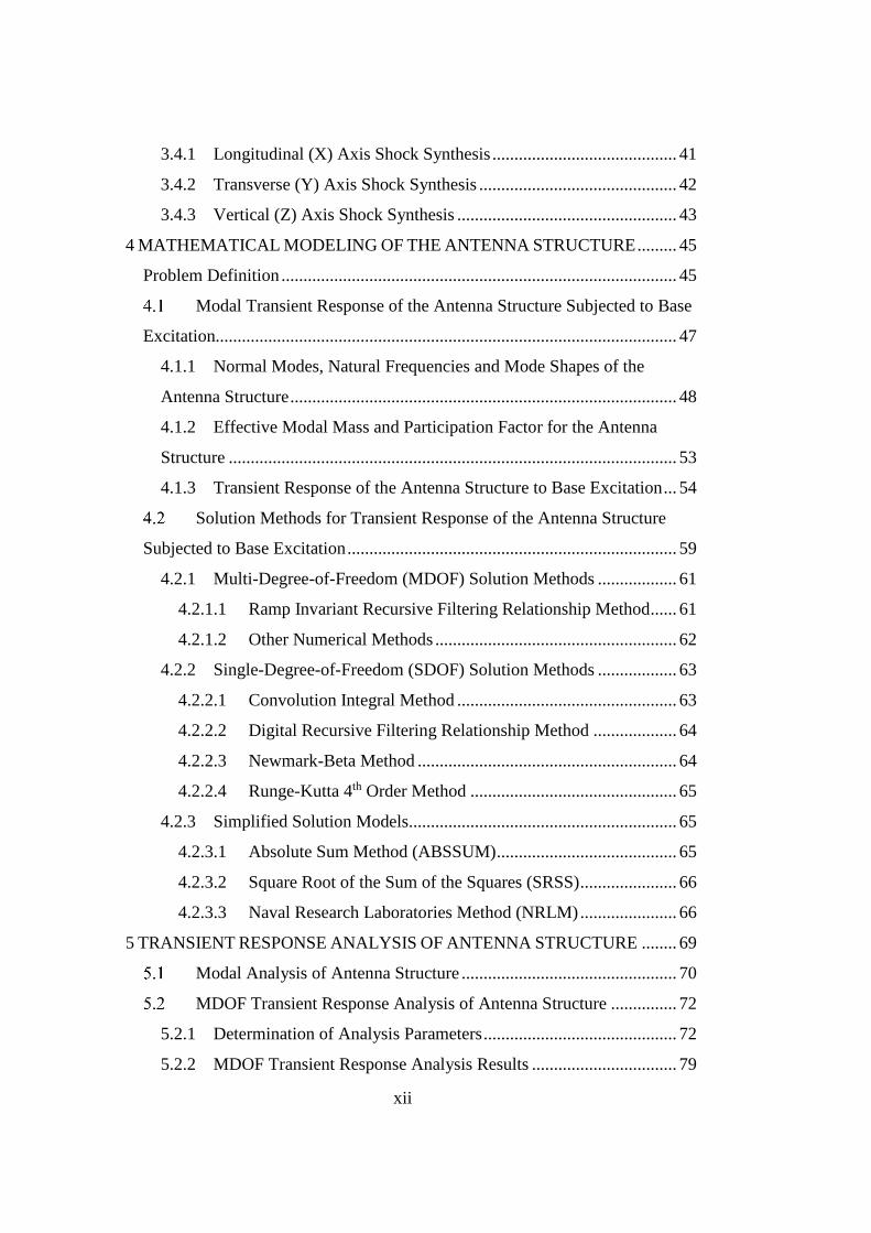
Figure 1. 3 Nomenclature of Shock Duration [5] ..................................................... 6
Figure 1. 4 Spring-mass System ............................................................................... 7
Figure 1. 5 El Centro, California, Earthquake of May 18, 1940; North-South
Component [6]........................................................................................................... 8
Figure 1. 6 Athwartship Velocity Time History measured on a Floating Shock
Platform nearby underwater explosion [6] ................................................................ 8
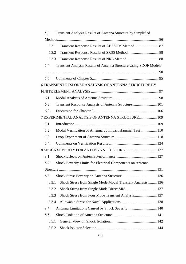
Figure 1. 7 Examples of shock pulses ...................................................................... 9
Figure 1. 8 Accelerated drop-table [8] ................................................................... 11
Figure 1. 9 USS OSPREY-MHC 51(left) [9] and CG 53(right-Courtesy of U.S
Navy) Ships Full-Scale Shock Trials ...................................................................... 12
Figure 1. 10 Underwater Antenna Platform ........................................................... 13
Figure 3. 1 Shock Response Spectrum Concept [38] ............................................. 30
Figure 3. 2 Shock Response Spectrum Model [23] ................................................ 31
Figure 3. 3 Free-body Diagram of SDOF System [23] .......................................... 31
Figure 3. 4 Time History of 40g 11ms Half-Sine Input Signal .............................. 34
Figure 3. 5 Acceleration Shock Response Spectrum for 40g 11ms Half-Sine Signal
................................................................................................................................. 34
Figure 3. 6 Shock Response Spectrum in four-way log paper [39] ....................... 35
Figure 3. 7 Shock Response Spectrum Regions [39] ............................................. 36

xviii
Figure 3. 8 General Form of Double Half-Sine Shock Acceleration-Time Signal 38
Figure 3. 9 Axis Definitions for Submarine ........................................................... 40
Figure 3. 10 Defined by BV043 (blue) and Synthesized (red) Shock Profile Shock
Response Spectrum for X Axis ............................................................................... 41
Figure 3. 11 Defined by BV043 (blue) and Synthesized (red) Shock Profile Shock
Response Spectrum for Y Axis ............................................................................... 42
Figure 3. 12 Defined by BV043 (blue) and Synthesized (red) Shock Profile Shock
Response Spectrum for Z Axis ................................................................................ 43
Figure 4. 1 Antenna Structure Attached to the Platform ........................................ 46
Figure 4. 2 Electrical Components Placed on Antenna Tip ................................... 46
Figure 4. 3 Antenna Model as a Cantilever Beam.................................................. 48
Figure 4. 4 Antenna Model Subjected to Transient Base Excitation ..................... 54
Figure 4. 5 Solution Methodology of MATLAB® Script Built for RFR Method . 62
Figure 5. 1 Three-Dimensional Model of Antenna Structure................................. 70
Figure 5. 2 First Four Bending Mode Shapes of Antenna Structure ...................... 72
Figure 5. 3 Shock Inputs Applied to the Antenna Platform ................................... 73
Figure 5. 4 Acceleration SRS for both Transverse Shock Inputs ........................... 74
Figure 5. 5 Relative Displacement SRS for both Transverse Shock Inputs ........... 75
Figure 5. 6 Comparison of transient acceleration responses of antenna structure
with respect to the number of modes included in the analysis ................................ 77
Figure 5. 7 Comparison of transient acceleration responses of antenna structure
with respect to the number of modes included in the analysis (Zoomed View) ..... 77
Figure 5. 8 Comparison of relative displacement responses of antenna structure
with respect to the number of modes included in the analysis ................................ 78
Figure 5. 9 Comparison of relative displacement responses of antenna structure
with respect to the number of modes included in the analysis (Zoomed View) ..... 78
Figure 5. 10 Time History of 200g 8ms Half-Sine Acceleration Input .................. 80
Figure 5. 11 MDOF Absolute Acceleration Response of the Antenna Tip ............ 81
Figure 5. 12 MDOF Relative Displacement Response of the Antenna Tip ........... 82

xix
Figure 5. 13 MDOF Relative Velocity Response of the Antenna Tip ................... 83
Figure 5. 14 MDOF Phase Portrait of the Antenna Tip ......................................... 84
Figure 5. 15 Histogram Plot for MDOF Absolute Acceleration Response ............ 85
Figure 5. 16 Histogram Plot for MDOF Relative Displacement Response ........... 85
Figure 5. 17 SDOF Absolute Acceleration Response of the Antenna Tip ............. 92
Figure 5. 18 Comparison of Absolute Acceleration Responses of the Antenna Tip
................................................................................................................................. 92
Figure 5. 19 SDOF Relative Displacement Response of the Antenna Tip ............ 93
Figure 5. 20 Comparison of Relative Displacement Responses of the Antenna Tip
................................................................................................................................. 93
Figure 5. 21 Comparison of Phase Portraits of the Antenna Tip ........................... 94
Figure 6. 1 First Mode Shape of the Antenna Structure (FEA Result) .................. 99
Figure 6. 2 Second Mode Shape of the Antenna Structure (FEA Result) .............. 99
Figure 6. 3 Third Mode Shape of the Antenna Structure (FEA Result) ............... 100
Figure 6. 4 Fourth Mode Shape of the Antenna Structure (FEA Result) ............. 100
Figure 6. 5 200g 8ms Half-sine Acceleration Input Defined to ANSYS® .......... 103
Figure 6. 6 ANSYS® Absolute Acceleration Response of the Antenna Tip ....... 104
Figure 6. 7 ANSYS® Relative Displacement Response of the Antenna Tip ...... 105
Figure 6. 8 ANSYS® Relative Velocity Response of the Antenna Tip ............... 105
Figure 7. 1 PCB PIEZOTRONICS® 086E80 Miniature Impact Hammer .......... 111
Figure 7. 2 IOTECH® Data Acquisition System ................................................. 111
Figure 7. 3 Antenna Attachment to the Experimental Set-up .............................. 112
Figure 7. 4 Hammer Test of Antenna Structure ................................................... 113
Figure 7. 5 eZ-Analyst Screen During Experiment .............................................. 114
Figure 7. 6 Measured FRF of Antenna Structure ................................................. 114
Figure 7. 7 Modal Analysis by ANSYS®® with tip mass................................... 116
Figure 7. 8 Response Curve Showing Half-Power Points and Bandwidth [44]... 117
Figure 7. 9 Drop Test Experiment ........................................................................ 120
Figure 7. 10 Shock Input Measurement Taken From Drop Table ....................... 121

xx
Figure 7. 11 Mathematical Model and Experiment Comparison ......................... 122
Figure 7. 12 FEA Model and Experiment Comparison ........................................ 123
Figure 7. 13 Frequency Content of Measured Data ............................................. 124
Figure 8. 1 Relative Displacement of the Antenna Tip ........................................ 129
Figure 8. 2 Electromagnetic Analysis of Dipole Antenna by HFSS® ................. 130
Figure 8. 3 Radiation Pattern HFSS® Analysis of Antenna with Maximum
Allowable Deformed Position ............................................................................... 130
Figure 8. 4 Relative Velocity Response of the Antenna from Updated Models .. 132
Figure 8. 5 Morse Chart for Mild Steel Beams [62]............................................. 133
Figure 8. 6 Component Bending on the Antenna Structure [63] .......................... 134
Figure 8. 7 Shock Damping by means of Isolators on, a) Acceleration-time plot,
b) Force-displacement plot [63] ............................................................................ 143
Figure 8. 8 Shock Velocity Formulation for Different Types of Shock [65] ....... 145
Figure 8. 9 Drop Experiment of Antenna with Isolator ........................................ 147
Figure 8. 10 Acceleration Response for the Antenna with Isolator ..................... 148
Figure 8. 11 Relative Velocity Response of the Antenna with Isolator ............... 149
Figure B. 1 General Specifications of IOTECH® WaveBook Data Acquisition
System ................................................................................................................... 169
Figure B. 2 General Specifications of PIEZOTRONICS® 356A01 Accelerometer
............................................................................................................................... 170
Figure B. 3 General Specifications of PIEZOTRONICS® 086E80 Impact Hammer
............................................................................................................................... 171
Figure B. 4 General Specifications of LANSMONT® PDT 80 Drop Table ....... 172
Figure E. 1 General Specifications of ATC® High Power Flange Mount Resistor
............................................................................................................................... 179
Figure F. 1 General Specifications of Taico ALPHA-GEL® MN Series Isolator
............................................................................................................................... 181

xxi
LIST OF SYMBOLS
A threshold pulse amplitude
0a maximum acceleration
cc critical damping constant
iC modal damping coefficient
D threshold pulse duration
0d maximum relative displacement
E modulus of elasticity
rese coefficient of restitution
n modal damping ratio
inf natural frequency (in Hz)
g gravitational acceleration
h no rebound drop height
rh drop height with rebound.
I area of moment of inertia
beamk beam stiffness
iK modal stiffness
L antenna length
m mass of the antenna

xxii
effm effective modal mass
iM modal mass
Q quality (amplification factor)
ˆnjq eigenvalue
eT effective shock duration
ET total shock duration
nT modal time variable
t time step
participation factor
V pseudo velocity
0V maximum pseudo-velocity
1V pseudo-velocity at shock event
1v velocity before impact
2v velocity after impact
w t base displacement function
n natural frequency (in rad/s)
iX modal acceleration response
nY x mode shape function
Y acceleration base input
maxiZ maximum modal relative displacement

xxiii
LIST OF ABBREVIATIONS
ABSSUM Absolute Sum Method
ASME American Society of Mechanical Engineers
COMINT Communications Intelligence
DDAM Direct Dynamic Analysis Method
DOFs Degree of Freedoms
EA Electronic Attack
EB Euler Bernoulli
ELINT Electronics Intelligence
EMP Electromagnetic Pulse
EP Electronic Protection
ES Electronic Support
ESM Electronic Surveillance Measurement
EW Electronic Warfare
FEA Finite Element Analysis
FEM Finite Element Model
FFT Fast Fourier Transform
IEEE The Institute of Electrical Electronics Engineers
IFF Identification Friend and Foe

xxiv
MDOF Multi Degree of Freedom
NRLM Naval Research Laboratories Method
PCB Printed Circuit Board
RFR Recursive Filtering Relationship
RMS Root-mean-square
RWR Radar Warning Receivers
SDOF Single Degree of Freedom
SIGINT Signals Intelligence
SRS Shock Response Spectrum
SRSS Square Root of the Sum of the Squares
UNDEX Underwater Explosions

1
CHAPTER 1
1INTRODUCTION
General: Electronic Warfare
Electronic warfare (EW) can be defined as any possible action that is possible with
the use of the electromagnetic spectrum or directed energy to control the spectrum,
attack an opponent, or obstruct enemy assaults via the spectrum [1]. The main
purpose of electronic warfare is to deny opponent attacks and ensure friendly
unrestrained access to the electromagnetic spectrum. Electronic warfare
applications can be seen in air, sea, land, and space applications for both manned
and unmanned systems as illustrated in Figure 1.1. Targets of the applications can
be humans, communications, radar, or other assets. In military applications,
electronic warfare is used to support military operations by means of detection,
denial, deception, disruption, degradation, protection, and destruction [2].
Figure 1. 1 Electronic Warfare Applications

2
Electronic warfare can be divided into three main subdivisions, namely, electronic
attack, electronic protection and electronic support. Electronic attack (EA)
applications are performed by active and passive ways. Active ways are jamming,
deception and active cancellation; passive ways are chaff, towed decoys, radar
reflectors and stealth. Electronic protection (EP) is also applied in active and
passive ways. As technical modification to radio equipment is an active way;
education of operators, enforcing strict discipline and modified battlefield tactics or
operations are passive ways of electronic protection. Electronic support (ES) can be
defined as an action of searching, interception, identification, and detection the
location of radiated electromagnetic energy sources for the purpose of immediate
threat recognition. Signals Intelligence (SIGINT), Communications Intelligence
(COMINT) and Electronics Intelligence (ELINT) are three subgroups of electronic
support applications.
Purpose of SIGINT is to collect and analyze of information from radar and
radio signals.
Purpose of COMINT is to listen into, analyze and decode the military radio-
traffic, teletype and fax signals.
Purpose of ELINT is to collect and analyze the radar, Identification Friend
and Foe (IFF), datalink, and missile firing signals. Radar Warning
Receivers (RWR) is one of the examples of these types of applications.
Apart from these classifications, radar technologies are another subgroup of
electronic warfare. The use of radar technologies is basically air-defense systems,
antimissile systems; marine radars to locate enemy ship, ocean surveillance
systems, outer space surveillance and rendezvous systems, guided missile target
locating systems so on.

3
(I) (II) (III)
(IV) (V) (VI)
(VII)
Figure 1. 2 Subdivisions of Electronic Warfare: (I)Very/Ultra High Frequency
COMINT,(II)Transportable V/UHF DF(Direction Finding),(III)Portable Jamming-
Electronic Attack,(IV)High Frequency-Electronic Attack,(V)Electronic Support-
ELINT,(VI)Submarine Electronic Surveillance Measurement,(VII) Air Defense
Search and Fire Control Radars

4
For all these electronic warfare applications; antennas, receivers, transmitters,
power unit, data collection and processing units, user interfaces and other residual
components are gathered up for the complete operation quality and performance.
Naval C-ESM/COMINT Antennas
The Institute of Electrical and Electronics Engineers (IEEE) defines the antenna as;
“An antenna is a device that provides a means for radiating and receiving radio
waves. In other words, it provides a transition from a guided wave or a
transmission line to a free space wave or vice versa” [3].
Antennas are the main components of electronic warfare applications mentioned in
previous section. Therefore, for different applications, different type of antennas is
possible to use. Naval ESM systems are the electronic warfare solutions in which
ELINT and COMINT solutions are tailored together. COMINT part of the system
consists of direction finding antennas and jamming antennas working in
communication frequencies. Direction finding antennas are built on strong support
masts and consist of dipole elements attached to the mast. These antennas are
responsible for the electronic support by means of detecting the position of threat
signal with minimum possible errors. Jamming antennas, on the other hand, consist
of long thin structures and printed circuit boards and the electronic components like
resistances, capacitances, baluns etc. attached. Jamming antennas use the reliable
information gathered by direction finding antennas and creates jamming signals to
those threats. Therefore, their main purpose is to create a disturbance signal when
the signal which is possibly a threat is detected. Jamming dipole antennas are one
type of antenna which can be used as Electronic Attack (EA) COMINT antenna.
The reason for the use of those antennas is to achieve required frequency band with
the certain amplitude and phase requirements. Jamming dipole antenna is a very
simple structure which is composed of long and thin metal electronic circuit boards
(or printed circuit boards). It is very vulnerable to vibration and shock especially

5
naval shock. Those types of antennas are used in field and on vehicle application
with competence without any extra precautions for shock. However in naval
applications; because of the shock levels reached in underwater explosions
(explained in following section), shock analysis and design for naval shock is a
must. In the scope of this thesis, the dipole jamming antenna subjected to
underwater shock explosion is investigated.
Mechanical Shock
Mechanical shock is defined as a non-periodic excitation of a mechanical system. It
is characterized by severity and suddenness that disrupts the equilibrium of the
system usually causing significant relative displacements [4]. These non-periodic
excitations can be caused by suddenly applied forces or by sudden changes in
magnitude or direction of velocity. Mechanical shock is usually expressed as a
single input pulse like half sine, saw-tooth, versed sine, triangular, rectangular and
other possible forms with peak amplitude(in acceleration or velocity) and duration
of the pulse. The duration of a shock pulse is the time required for the acceleration
of the pulse to rise from some stated fraction of the maximum amplitude and to
decay to this value. 𝑇𝐸 is the “shock duration” which can be defined as the
minimum length of time containing all time history magnitudes more than absolute
value which is one-third of the shock peak magnitude absolute value, 𝐴𝑝. On the
other hand, 𝑇𝑒 is the “effective shock duration” which can be defined as the
minimum length of continuous time that contains the root-mean-square (RMS)
time history amplitudes more than the value which is one tenth of the peak RMS
amplitude related to the shock event and the averaging time for the unweighted
RMS computation is assumed to be between one tenth and one fifth of 𝑇𝑒 [5].

6
Figure 1. 3 Nomenclature of Shock Duration [5]
Sources of input pulses can be various. The well-known examples are drop,
underwater explosion impact, ballistic impact, collision impact, gunfire,
transportation, aircraft or missile maneuvers etc. The effects of mechanical shock
created by these sources can be so severe that the system stores the high value of
energy within a short period of time and releases it over a longer period of time
with comparably lower peak value. If the peak value is held below limits with the
extension of release time, the shock effect consequences may not be that harsh and
harmful for the system. For analyzing the equipment such as antenna subjected to
shock or vibration, it is convenient to represent the antenna as a spring mass system
shown in Figure 1.4. In this case, transient force f(t) is applied to a foundation
which supports the antenna. It is mounted on to a base with a spring of stiffness k
and a damper with damping c. The response characteristics of the antenna to such a
loading have a relationship between the frequency of the applied transient force and
the natural frequency of the system.
7
Figure 1. 4 Spring-mass System
If the spring is very stiff and the damping is small, the response of the antenna will
be almost the same as the motion of base. If natural frequency of the system and
the frequency of the transient force is nearly the same, the response of the
equipment is much greater than the motion of base. If spring is very soft, the
response of equipment has lower amplitude and longer duration motion than the
base. As seen from these cases, the determining factor with respect to the shock
response is the frequency relationship between the input and the system. Measured
shock environments in the real world are usually presented in motion-time histories
as illustrated in Figures 1.5 and 1.6.

8
Figure 1. 5 El Centro, California, Earthquake of May 18, 1940; North-South
Component [6]
Figure 1. 6 Athwartship Velocity Time History measured on a Floating Shock
Platform nearby underwater explosion [6]
These measurements produce very complex curves that are very difficult to
describe with mathematical terms. They cannot easily created in laboratory testing
conditions. In order to achieve test requirements to simulate real life conditions,
shock pulse is a desirable and convenient way to describe shock. Several ideal
shock pulse shapes are displayed in Figure 1.7. These shock pulses are described
by representations of acceleration as a function of time. They can be easily
9
reproduced in one laboratory to another. Furthermore, there are mathematical
equations for describing these pulses in terms of any motion parameters.
Types of classical shock pulses are namely; square, half-sine, haversine, triangle,
quarter-sine, sawtooth and parabolic cusp. Classical shock inputs are accepted and
used for shock profile synthesis in MIL-STD-810G testing standard [5]. Another
way of describing shock pulses are shock response spectra. Shock response
spectrum concept will be discussed in following chapters. There are also types of
shock inputs like pyroshock, which is short duration, high acceleration shock pulse
and seismic shock which is low acceleration, long time, and high displacement
shock input [7].
Figure 1. 7 Examples of shock pulses
Shock phenomenon is described as dynamic occurrence whose duration is short
relative to the natural frequency of the system excited. Such effects can be caused
by several sources. Handling, transportation and shipment are the most common
sources of shock. Shock created during coupling of rail cars or cargo handling
procedures can be the examples of these types of shock sources. Drop shock is

10
another special case of shock sources. During manufacturing processes machines or
other heavy equipment may produce shock loading that may damage nearby
equipment. Ballistic impact, collision impact and explosive shock are the sources
that can usually be encountered in military applications. Blast impacts, landing of
aero-vehicles, pyrotechnic excitation and earthquakes are among other type of
sources. In particular for this thesis, the most important source is underwater
explosions near ships and submarines producing a very serious shock environment.
Considering the magnitudes and durations of the shock sources mentioned above,
they show variety of shock effects from one application to another.
Table 1. 1 Shock Effects of Various Shock Pulses [6]
Shock testing is very important to simulate the shock environment in laboratory
conditions in proper and reliable manner. For different shock environment,
Richter Scale Magnitude 6.5
Maximum possible shock
6000 ft
Parachute landing
Fall into fireman's net
Approximate survival limit with well distributed forces (fall
into deep snow bank)
Adult head falling from 6ft onto hard surface
Voluntarily tolerated impect with protective headgear
Pyrotechnic Shock (Stage Operation):
Average in "fast service"
Comfort limit
Emergency deceleration
Normal acceleration and deceleration
Emergency stop braking from 120 kph
Very undersirable
Maximum obrainable
Crash (potentially survivable)
Ordinary take-off
Catapult take-off
Crash landing(potentially survivable)
Underwater Shock:
Seat ejection
Parachute opening-40000 ft
Comfortable stop
Earthquake:
Man:
Aircraft:
Automobiles:
Public transit:
0.007
0.02
20-30
20-30
0.001-0.1
0.0001-0.001
0.2-0.5
0.5
0.1-0.2
0.1
0.015-0.03
3
0.1
10-40
1.5
0.25
0.25
250
18-23
1-5
1-5
1-5
5
2.5
3-5
3-5
Head:
0.5
1.0
40-2000
100-15000
200
10-15
33
8.5
3-4
20
0.7
20-100
0.5
2.5-6
20-100
0.1-0.2
0.3
2.5
0.1-0.2
0.4
0.25
0.45
Type of Operation Acceleration (g) Duration (sec)
Elevators:

11
different test methods should be selected. Determining factors of these methods are
shock amplitude, shock duration and the dimensions of to-be-tested part. Shock
testing methods can be classified as following [8].
Simple Shock Pulse Machines
o Drop Tables
o Air Guns
o Vibration Machines
Complex Shock Pulse Machines
o High-Impact Shock Machines
Lightweight Machines
Medium-Weight Machines
Heavy-Weight Machines
o Hopkinson Bar
Multiple Impact Shock Machines
Rotary Accelerator
Figure 1. 8 Accelerated drop-table [8]

12
Ship Shock and Underwater Explosions (UNDEX)
The earliest naval mines were designed to breech the hull of a ship below the
waterline and cause flooding. Over years, underwater warfare became more
complicated and turned to water delivered and air delivered torpedoes, air delivered
bombs, contact and influence mines and anti-ship missiles etc. Following years,
especially after the World War II, navies studied on to understand the phenomena
of underwater explosion and develop design methodologies to reinforce ships
against the threat. Because, the effects of such explosions may collapse the whole
structure of ships and submarines, or may cause severe damages to electronic
equipment, warfare technologies or structural parts. Machinery and equipment for
naval application must be designed to operate under these severe conditions. The
shock conditions for naval applications are more severe than most of the other
military operations like tanks and airplanes. Therefore, shock competitive
ship/submarine design, component survival precautions and shipboard design
improvements have become primary issues for underwater explosion survival.
Figure 1. 9 USS OSPREY-MHC 51(left) [9] and CG 53(right-Courtesy of U.S
Navy) Ships Full-Scale Shock Trials

13
Motivation
COMINT high gain dipole antenna designed for electronic warfare is used on a
submarine platform as a part of a C-ESM/COMINT system. Therefore, the
complete system is to be operating with underwater platform requirements. In order
to meet these requirements, the design considerations, analysis, tests and
qualifications should be performed.
Figure 1. 10 Underwater Antenna Platform
Underwater shock disturbances may cause some malfunctions to antenna structure.
In electromagnetic point of view, shock may cause changes in material dielectric
strength, variations in magnetic and electrostatic field strength; material electronic
circuit card(or board) malfunction, damage or electronic connection failure and

14
material failure as a result of increased or decreased friction. In mechanical point of
view, shock may cause permanent mechanical deformation as a result of overstress
of material, collapse of mechanical elements as a result of ultimate stress of the
material being exceeded, accelerated fatigue of materials and material failure as a
result of cracks, delamination or fracture of radome (radar-dome; composite, high
strength mechanically protection material which allows electromagnetic waves to
pass).
Because of these impending harmful consequences of shock disturbances on
antenna structures mentioned above, customers require antenna structure (as the
whole ELINT system) to endure operations without any failure, therefore, to pass
certain quality assurance tests compatible with pre-specified military standards. In
order to design a structure that can withstand to shock pulses or qualify the
antennas designed before, and if necessary take shock isolation precautions for the
system, complete shock analysis is essential.
Scope, Objective and Contribution of Work
In the scope of this thesis, shock analysis of the antenna structure subjected to
underwater explosions is performed. Complete shock analysis consists of
determination of underwater shock characteristics, analytical solution of shock
phenomenon, finite element model solutions of shock phenomenon, shock testing
and shock isolation of the antenna structure with the platform.
Design specifications of naval electronic warfare applications for foreign customers
contain harsh naval shock survival criterion. Therefore, mechanical structures of
those systems should withstand and pass laboratory test for naval shock.
Preliminary design considerations should be taken and further actions should be
carried with those shock analysis and tests beforehand. Thus, underwater explosion
shock (UNDEX) should be analyzed analytically and should be qualified with
15
finite element models and experiments. Most of the customers of those C-ESM
systems are foreign and since defense test method standards like MIL-STD-810F/G
used in military applications do not contain underwater shock inputs and testing
methods, other standards such as BV043 or STANAG are taken as reference.
Therefore, shock inputs and testing methods are determined by shock profile
synthesis of those standards into possible frequently used signals and methods.
Mathematical model of antenna structure is built both SDOF and MDOF point of
view. For these models, solution techniques and faster solution algorithms are
provided. Pre-defined and synthesized shock pulses are used as input signals to
solve those equations. Finite element model that describes the phenomenon is
created for the problems analytically solved before. These finite element model
verifications can be the guide for complex geometries that are very hard to build
complete analytical model. Further, those analytical and mathematical models are
validated with experiments. As shock loadings are very harmful for electronic
components, isolation of the structure is needed. Therefore, shock isolation
techniques are investigated and isolation alternatives are compared. Since
commercial products do not meet the electrical requirements of antenna, a shock
isolator for the antenna structure is designed. Analytical solution, finite element
analysis and experiments are performed for this isolation case, afterwards.
Analytical and finite element model can be used instead of experimentally difficult
verifications, as experiments of shock cases with high impact short time duration
for big and bulk mechanical parts are very hard. Similarly, experimental analysis
can be used instead of analytical or FE models when the system consists of
elements that are hard to model like composite structures, isolator or other non-
linear elements. Therefore, this study contains all possible ways for underwater
shock analysis and design that can serve guidance for designers from preliminary
designs to post-failure isolation problems.

16
Outline of the Dissertation
In chapter 2, background and literature surveys on topics relevant to the study are
presented.
In chapter 3, shock profile synthesis is performed and shock inputs are determined
with respect to the project requirements. Shock profiles are synthesized from
BV043 standard into classical shock inputs which are capable to be performed in
laboratory conditions.
In chapter 4, mathematical modeling of an antenna structure as a cantilever beam
will be performed. Modal analysis using Euler-Bernoulli Beam Theory is used for
continuous modeling of antenna structure. Then, transient response of the antenna
to shock impulse is examined and integrated to mathematical model.
In chapter 5, results of mathematical built for antenna structure is presented. Multi-
degree-of-freedom transient shock analysis using mathematical model is examined
in detail and solutions of simplified models are presented. Finally, success of
MDOF model is discussed and comparisons between alternative solution methods
with MDOF are observed.
In chapter 6, transient finite element analysis of antenna structure is performed by
means of ANSYS®. Modal analysis results and transient responses of antenna is
presented and compared with mathematical model solutions.
In chapter 7, experimental analysis of antenna structure is performed. Mathematical
model results and finite element analysis results are compared with experimental
analysis results in order to observe accuracies for validation of these models.
In chapter 8, antenna performance criteria are discussed from both electromagnetic
and mechanical point-of-views. Shock isolation theory is explained and shock
isolation of antenna structure is performed. Finally, validations of isolation
elements are performed by experimental analysis.

17
In chapter 9, results are summarized and evaluated together, while conclusion is
drawn including the recommendations for future work.

18

19
CHAPTER 2
2LITERATURE SURVEY
Historical Background
Theoretical and experimental studies dealing with shock are totally related to the
basic laws of dynamics and fundamentals of vibration. Therefore, it is vital to
mention about few developments about dynamics in general and particularly
vibration. It is believed that the serious study on vibration has begun with Galileo.
In his, “Discourse Concerning Two New Sciences” [10] published in 1638,
fundamental law of oscillating pendulum is illustrated and the new phenomenon
“resonance” is introduced. In the same years, Christian Huygens worked on
compound pendulum with the analysis of restricted motion along a circular path
and the theory of wave propagation.
Hooke’s search on stress and strain and Descartes’ development on the Cartesian
coordinate system were important contributions on vibration analysis. However,
Isaac Newton suggested the milestone law, namely the second law of motion,
which is the basis of almost all vibration related equations of motions. Following
Newton’s teachings about calculus use on vibratory problems, several
mathematical techniques that advanced vibration analysis are introduced. Among
them, Taylor Series is useful in response calculations, D’Alambert principle is
applied to forced vibration problems and Lagrange equations are used to express
equations of motion in terms of energy principle.
Principle of superposition was published by Daniel Bernoulli in 1755. Fourier, on
the other hand, extended the principle and applied it to the theory of oscillations.
20
Fourier also proved the theorem, Fourier Transform, which states that any periodic
function can be represented as a sum of sines and cosines.
Lord Rayleigh integrated all available information about sound and vibration and
published the first complete, formal and useful presentation on sound and vibration.
Up to and including the Rayleigh era, sound and other vibration phenomena were
treated together. Beginning in the 20th century, specialization of vibration began
and some of the sub-specialty categories like vibration engineering, flutter
engineering, acoustical engineering are introduced. The first modern dissertation
about mechanical vibration was written by Timoshenko including the topics as
understanding of vibration, vibration isolation, vibration influence on fatigue life,
vibration monitoring and so forth.
Although it is not certain, mechanical shock term was used to refer the need of
specific areas compatible with the development of technology. With those
developments in technology, military equipment is likely to withstand harsh effects
of environments produced during warfare. For example, During World War I,
shock testing machine for testing shipboard equipment to survive shock produced
by the blast from ship guns was developed. With the necessity of detailed
considerations of shock related phenomenon, some organizations like Shock and
Vibration Information Center, Shock and Vibration Information Analysis Center
were founded; several technical papers on shock problems are published in the
proceedings of professional societies like ASME, IES and etc. , shock and vibration
symposia and other specialized societies. Important textbooks in the field like The
Shock and Vibration Digest, Harris’ Shock and Vibration Handbook and Shock
and Vibration Bulletins are published.

21
Literature Survey
In the study, numerous sources in literature were reviewed. Reviews were focused
on shock concept, shock response spectrum theory, calculation of shock response
spectrum, single degree of freedom and multi degrees of freedom mathematical
modeling of shock, underwater shock phenomena, cantilever beam theories,
numerical solutions of multi degrees of freedom shock, continuous modeling of
cantilever beams, finite element modeling using commercial software like
ANSYS®, shock testing methods, shock isolation and other topics relevant to the
study. Only limited part of those sources are included to literature survey part for
brevity.
The concept of shock spectra was first introduced in a printed manner by Maurice
Biot [11-13]. He focused on the damage potential of earthquake motions. He
defined earthquake spectrum (or response spectrum) as the maximum response
motion from the series of single degree of freedom oscillatory systems in the
frequency range of interest. In his PhD. Thesis [14], Biot showed the effective
number of modes to be interested for design concerns. He focused on earthquake
motions and he used the assumption that dynamic motion of the building does not
affect ground’s motion; however, studies demonstrated that this assumption is very
conservative.
Mindlin [15] suggested that this response spectrum approach can be used for
general types of shock motions. He suggested that damage potential of different
shock motions can be compared with this method. Later, Housner [16] developed
the first seismic spectra that can be attained by averaging of eight ground motion
records. These records were obtained two each from following earthquakes, El
Centro(1934), El Centro(1940), Olympia(1949) and Tekiachapi(1952).
Newmark [17], on the other hand, used the amplification factors applied to maxima
values of ground motions respectively and used them to create earthquake design
spectrum. In this spectrum, for different probabilities of occurrence and a range of

22
damping of the structure, amplification is listed. He also presented the relation for
development of spectrum from ground motion maxima. Shock spectrum level
becomes maximum ground acceleration level at relatively high frequencies which
is the aforesaid feature seen in El Centro earthquake. Newmark [18] also proposed
the series of single step integration methods to solve structural dynamic problems
especially for blast and seismic loading. However, Newmark’s methods have been
applied to various dynamic analysis problems. Moreover, these methods have been
improved and modified by researchers working in similar areas of structural
dynamics applications.
Alexander [19] published a paper as a basic overview of a shock response spectrum
containing the definition and history of shock response spectrum. He also summed
up the events characterized by shock response spectrum and added milestone
examples of those events. He also discussed the shock response spectrum analysis
of linear multi-degree-of-freedom structures. He presented the formulation that
used mode superposition in conjunction with shock response spectrum and
estimated the maximum dynamic response of a linear system without solving the
transient multi-degree-of-freedom equations of motions. Alexander also presented
the history and development on naval shock design spectra specifically.
Tuma and Koci [20] proposed the new method of shock response spectrum
calculation related to an acceleration signal which excites the resonance vibration
of substructures. The maximum or minimum of the substructure acceleration
response is determined by shock response spectrum as a function of the natural
frequencies by means of a set of the single degree of freedom systems modeling for
those substructures mentioned. The shock was recorded as acceleration signal in
digital form and IIR digital filter was used to approximate the single degree of
freedom systems. Then filter response corresponding to the sampled acceleration
signal was straightforwardly calculated. Thus, the excitement partition of
individual component of the impulse signal to the mechanical structure to resonate
can be easily monitored by means of shock response spectrum.

23
Smallwood [21] simulated the improved recursive formula for calculating shock
response spectra. The aim of this study is to enhance the recursive formulas that are
based on impulse invariant digital simulation of a single degree of freedom system
since the results of such simulations contain significant errors when the natural
frequencies are greater than one sixth of the sample rate. To do this, one more filter
was added to recursive filter and good results were obtained over a broad frequency
range even for the frequencies exceeded the sample rate.
Kelly and Richman [22] shed light on some physical descriptions and mathematical
representation of the shock response spectrum. This article has been taken as a
reference and guidance in numerous books on the similar subjects and research
studies. The main idea of this study was to correct several typographical errors in
the Biot’s presentation of a recursive algorithm for shock response spectrum
calculations. Another purpose of this study was to present a MATLAB®
implementation of the corrected algorithm.
Irvine [23] presented a complete study on shock response spectrum. In the study,
he defined shock response spectrum and illustrated its physical meaning with real
case examples. Irvine modeled the shock response spectrum and showed half sine
and pyrotechnic impulse examples which are converted from time history to
response spectrum. In this study, Irvine also derived the time response of the single
degree of freedom system subjected to shock input. Calculating time response of
the system, Z-transform method [24] was introduced for both acceleration and
force shock cases. For calculating frequency domain solutions, Fourier spectra
method is introduced. Irvine also gave significant information about the error
sources of data collection of shock events, shock response spectrum slope and
component qualification test methods in this study. In another study of Irvine [25],
shock response of multi-degree-of –freedom systems are investigated. In this study,
approximation methods that can simulate multi-degree-of-freedom system as the
summation response of a series of single-degree-of-freedom systems are presented
namely Absolute Sum, Square Root of the Sum of the Squares, Naval Research

24
Laboratories method. Results of these methods are compared to the mode
superposition method on a simple example.
Parlak [26] performed an experimental analysis of the shock produced by repetitive
recoil shocks due to machine gun firing. Integrated circuit piezoelectric
accelerometers ware located four predetermined points in order to test the shock
and vibration on the system. In order to define minimum shock profile that the
electronic components can survive, shock response spectrum analysis was
performed. The aim of the study was to use those equivalent shock profiles for
shock qualification testing of similar equipment located on military low level air
defense system.
Burgess [27] performed a study as a PhD. thesis on the use of experimental modal
analysis techniques with Fourier transform methods in order to apply on the
transient response analysis of structures. Primarily, linear structures were taken into
consideration to examine the limits and validity of the approach. At the same time,
errors related to the time aliasing within the inverse Fourier transform was derived.
Several experimental procedures for modal analysis were applied to demonstrate
the method on a beam structure. Further, the applicability of the same analysis and
prediction techniques was explored. Prediction methods included using specific
linear models and developing non-linear models that describe transient response.
Linear multi degree of freedom systems were also examined in the scope of the
study and structural nonlinearity was added to the models as concentrated single
component.
Bhat et. al, [28] applied shock response spectrum analysis approach to obtain
optimum design parameters for electronic devices. Bhat performed the analysis
using commercial software ANSYS® and obtained the results of dynamic analysis
of printed circuit board (PCB) in order to use for designing compliant suspension
and cushions.

25
Wang et. al [29] created the mathematical modeling and mechanism analysis of a
novel heavy-weight shock test machine simulating underwater explosive shock
environment. They also performed numerical solutions to evaluate the limitations
of shock test machine under various shock velocity inputs. The proposed test
machine can produce nearly the same pulse forms as noted in standards as
BV043/85 OR MIL-S-901D. The proposed system and mathematical model
provided theoretical basis and design techniques.
Campos [30] showed the great correlation between analytical and experimental
results using Euler-Bernoulli theory and finite element analysis to solve shock
impulse acting on cantilever beam. Based on these correlations, Campos modeled
the blade of an impeller as a cantilever beam and found out the mode shapes and
natural frequencies to use this information for preliminary bladed impeller design.
He also analyzed the mixed flow fan under ballistic shock impact by means of
finite element analysis and classical theory in order to illustrate real system
responses to shock loading with help of Full Method and Mode Superposition
Method. Campos also investigated the effects of variation pulse width in the
acceleration input while he was analyzing the shock loading under simple
continuous structures using finite element analysis.
Haukaas [31] derived the fundamental governing differential equations for Euler-
Bernoulli type beams namely equilibrium and section integration, material law and
kinematics. He extended the study bending analysis, specifically, shear stress in
bending and bi-axial bending for different type of structures with different cross-
sections. He also explained the shear centre concept for both open cross-sections
and closed cross-sections.
Yang [32] provided an interactive handbook containing formulas, solutions and
MATLAB® toolboxes for stress, strain and structural dynamics problems.
Fundamental terms like beam types, boundary and initial conditions, response time,
effective excitement time, damping, modal damping and output control were
introduced. Static analysis of Euler-Bernoulli (EB) beam was explained in order to

26
give useful information that will be the background of dynamic analysis. In
dynamic analysis part, mode shapes of EB beams, time response and state space
response of beams and internal forces were presented along with the governing
equations and analytical solutions.
Remala [33] presented an overview of numerical integration methods for the
solution of linear equations. In the study, central difference method, Newmark time
integration method and Newton-Raphson were included. A simple example to
calculate the response of spring-mass system were calculated using both central
difference and Newmark method in order to illustrate how the methods are
implemented to any vibration problem. Remala also presented general information
about Newton-Raphson method as an implicit numerical integration method to
solve nonlinear structural problems.
DeBruin [34] discussed the potential error source created by shock-isolation
systems and provided a guideline to make configuration planning to ensure system
performance, installation and operation of an antenna system. He explained the
potential source of error the shock-isolation systems such as wire rope isolators or
encapsulated wire rope selected to make system survive from the shock
requirements of tracked vehicles, vehicles supporting large-caliber cannons and
armored vehicles subjected to ballistic shock.
Parlak [35] studied the shock and vibration isolation of machine gun firing where
machine gun together with isolator is located on a military platform. First
predefined isolator on the system was used for field test in order to determine
shock levels on the system. Then, a mathematical model compatible with the
experimental result was built. Making some changes in the parameters of the
model, it was possible to improve the model to simulate real world situations.
Moreover, the study investigated the calculation of shock levels to test the
materials which are subjected to repetitive shock pulses. SRS analysis was done to
define shock specifications of the some equipment on the military platform.

27
Klembczyk [36] provided a guideline on numerous methods and applications of
implementing isolation, shock absorbing and damping to dynamic systems and
structures. Shock, vibration and structural control problems can be solved
essentially with successful integration of these tools. Therefore, with this study,
Klembczyk aimed to equip the engineers with basic understanding of isolation
system attributes that have been proven to be reliable and effective to solve great
amount of the shock and vibration isolation applications.
From these literature survey process, useful information about SRS calculation
methodology and formulation is used especially sources from Biot [11-13] and
Alexander [19]. As a solution alternative, Digital Recursive Filtering Relationship
method and its applications are learned along with case studies [20-24]. During the
modeling process of antenna structure as cantilever beam with Euler-Bernoulli
Theory, various sources are scanned and useful information are extracted from
these as presented in following chapters in detail [30-34, 36]. For MDOF transient
analysis procedure, modal transient related topics are scanned along with Ramp
Invariant Digital Recursive Filtering Method [23-25, 28]. Shock isolation for
components are another important issue which is researched much. Useful
information about shock isolation theory, methodology and case studies are found
from literature [34-36]. Apart from these sources mentioned, some other sources
are used for certain throughout the study in mathematical modeling chapter. The
information exerted from these sources are presented in appropriate parts of the
chapters while discussing the importance of those within the methodologies.

28

29
CHAPTER 3
3SHOCK PROFILE SYNTHESIS
Theory: Shock Response Spectrum
In order to represent the input pulses or monitor the effect of shock motion on a
structure, either the form of time history or commonly used form, namely, shock
response spectrum (SRS) is used. While shock isolation, shock hazard monitoring;
displacement, velocity and acceleration responses are represented generally in time
domain, SRS can be used to verify a structure or a device can support transient
disturbances encountered during its real life operational or environment conditions.
“A Shock Response Spectrum is a plot of the peak responses of an infinite number
of single degree of freedom systems to an input transient” is the accepted definition
of SRS [37]. The degree of freedom can be defined as the ability of an object to
move along or around only one axis and these independent degree-of-freedoms
(DOFs) are selected as references to analyze transient phenomena. Instead of
analyzing these DOFs in Fast Fourier Transform (FFT) process, the SRS is
introduced as another mathematical tool inherently by this SDOF reference. Indeed,
FFT algorithm is not well-matched to non-stationary signals of short duration. Due
to the shortness of these oscillations, the severity can be characterized by their
maximum effects on the SDOF set.
Even though the selected SDOF reference does not represent the equipment to be
tested, one can assume that if two different excitations have the same severity
(SRS), they will induce equivalent effects on this equipment. The notion of
equivalence is that using synthesized pulse can replace complex or hard-to-generate
excitation whose severity is the same. Typical examples can be simulation of

30
gunfire, seismic shock, underwater explosions, aircraft taking off, and so. Shock
response spectrum is a useful tool for estimating the damage potential of a shock
pulse, as well as for test level specification. MIL-STD-810F/G requires this format
for certain shock environments.
As stated above, the shock response spectrum assumes that the mathematical shock
pulse is applied as a common base input to a group of independent single-degree-of
freedom systems as shown on Figure 3.1. The peak responses of each system for
corresponding natural frequencies are given on SRS curves. In earlier applications,
unless otherwise specified, systems are taken as undamped. However, damping is
generally fixed to a constant value, such as 5% which is equivalent to an
amplification factor of 10 [23].
Figure 3. 1 Shock Response Spectrum Concept [38]

31
The shock response spectrum model can be drawn as following form given on
Figure 3.2 as a complete series of single-degree-of freedom (SDOF) systems. For
the system, �� is the common base input while ��𝑖 is the absolute response of the
each system to the input mentioned. 𝑀𝑖 represents mass, 𝐶𝑖 represents damping
coefficient, and 𝐾𝑖 represents stiffness for each system, while 𝑓𝑛𝑖 represents natural
frequency.
Figure 3. 2 Shock Response Spectrum Model [23]
Applying Newton’s law of motion to a free body diagram of an individual system,
following one-degree-of freedom is modeled.
Figure 3. 3 Free-body Diagram of SDOF System [23]

32
According to the free-body diagram, following governing differential equation of
motion can be written:
mx cx kx cy ky (3.1)
Defining relative displacement as z=x-y and substituting this into (1), following
equation is obtained.
mz cz kz my (3.2)
Natural frequency (𝜔𝑛), critical damping constant (𝑐𝑐) and damping ratio (ξ) are,
n
k
m (3.3)
2 2 2c n
kc m km m
m (3.4)
c
cc
(3.5)
Furthermore, ζ is often represented by the amplification factor or quality Q, which
is defined as = 12ξ⁄ .
Substituting these terms into (2), equation of motion becomes,
22 n nz z z y t (3.6)
Equation (3.6) does not have a closed form solution for the general case in which
��(𝑡) is an arbitrary input function. Therefore the problem should be solved by
convolution integral approach. After that, convolution integral is to be transformed
into series for the case ��(𝑡) is converted to a form of digitized data. Then, these
digitized series of data is to be converted to a digital recursive filtering relationship
to accelerate the calculation. The resulting formula for the absolute acceleration is
given in Equation (3.7) as follows.

33
1 2
2
1
2exp cos exp 2 2 ...
exp 1 2 sin 2 cos
i n d i n i n i
nn n d d i
d
x t t x t x ty
t t t t y
(3.7)
where,
1d n (3.8)
Z-transform theory approach is described in many control systems or signal
analysis textbooks. For this calculation Dorf, R. [24] is taken as reference. The
derivation of the complete formulation is taken from Irvine’s paper [23].
Equation (3.8) can be used to calculate the shock response spectrum. One should
use this equation for each natural frequency to extract complete spectrum values.
Equation (3.8) can be calculated via computer program such as MATLAB®,
FORTRAN, and C/C++. In order to apply further synthesis calculations in this
chapter, MATLAB® script is prepared. For the calculations damping ratio can be
taken as constant for each degree-of-freedom as Q factor.
The alternate method, Fourier transform, can also solve the Equation (3.6);
however frequency domain solution is not that useful for shock response spectrum
applications. Therefore, digital recursive filtering approach is the best and fastest
way to calculate the whole spectrum.
The example for an arbitrary half-sine input (Figure 3.4), Acceleration SRS is
given in Figure 3.5. For this input (40g 11ms half-sine), frequency interval is
scanned from 1 Hz to 10000Hz, with the modal damping factor value Q=10.
Response is plotted on log-log scale in order to observe the wide range of response
values together.

34
Figure 3. 4 Time History of 40g 11ms Half-Sine Input Signal
Figure 3. 5 Acceleration Shock Response Spectrum for 40g 11ms Half-Sine Signal
0 0.005 0.01 0.015 0.02 0.025 0.03
0
5
10
15
20
25
30
35
40
Time(sec)
Accele
ration (
G)
Time History of Acceleration Input
40 g 11 ms Half-sine Input
100
101
102
103
104
105
100
101
102
Peak A
ccele
ration (
G)
Natural Frequency (Hz)
Acceleration Shock Response Spectrum

35
Shock Response Spectrum for Naval Applications
Shock response spectrum for naval applications is shown in logarithmic graph
containing velocity, acceleration and relative displacement information together as
shown in Figure 3.6.
Figure 3. 6 Shock Response Spectrum in four-way log paper [39]
In Figure 3.6, d represents the maximum relative displacement of the single-
degree-of-freedom system, a represents the maximum shock response acceleration
obtained for shock input. The value of maximum acceleration in time history is half
of the value of the acceleration value in spectrum. V is defined as pseudo velocity,
because the relation (3.9) between velocity, acceleration and relative displacement
is the approximate solution. The exact solution contains complex formula, this
approach is preferred. Therefore, V is defined as pseudo velocity. In equations and
the response spectrum, ω represents the corresponding natural frequency. The
relation between velocity, acceleration and relative displacement is given below:

36
2a V d (3.9)
Investigating the typical naval shock response spectrum (Figure3.7), following
properties of the spectrum is observed. The single-degree-of freedom system
behaves highly resistive at high frequency region, namely REGION A. At this
region spectrum has the maximum acceleration amplitude. At middle region of
spectrum, the resonant region corresponding to shock input (REGION B). At lower
frequencies, spectrum has almost constant velocity line. This frequency region
(REGION V) is defined as velocity change region. The shock input related to this
region can be defined as impulsive step velocity change. At the very left part of the
spectrum (REGION D), relative displacement is dominant. Therefore, spectrum has
maximum displacement value among the whole response spectra [39].
Figure 3. 7 Shock Response Spectrum Regions [39]

37
Determination of Assessment Criteria from Shock Response Spectrum
BV043 standard [39] is the building specification for ships of the German federal
armed forces standard. MIL-S-901D [70] standard is a military specification for
High Impact mechanical shock which applies to equipment attached on naval
platforms. In this standard, shock qualification criteria of the structure is defined
with shock testing procedures like full-scale ship/submarine tests and floating
barge test. Since MIL-STD-810F/G does not cover any naval shock or underwater
explosion testing standard, and in Turkey there is no facility to perform MIL-S-
901D testing standard requirements, the equivalent, even harder to perform
standard BV043 is typically taken as reference for naval projects, as a demand of
customers. In BV043 standard, the shock loadings to act on the equipment attached
on standard surface ship and submarine are defined briefly. It is possible to
calculate standard time equivalence of the shock signal whose spectrum value is
already known by means of BV043. In standards, generally, half-sine or saw-tooth
shock forms are used because these types of forms are easy to be generated in
laboratory conditions, as double half-sine form is used to in BV043 standard. In
following part, double half-sine shock time shock signal determination process is
presented. In order to define time input, 𝑎2, 𝑎4, 𝑡1, 𝑡2 and 𝑉1 values should be
calculated using tabulated 𝑎0, 𝑉0 and 𝑑0 values from standard.

38
Figure 3. 8 General Form of Double Half-Sine Shock Acceleration-Time Signal
In standard following derivations are explained. The amplitude of the positive half-
wave has to amount of half the maximum acceleration, 𝑎0. The surface below the
each half wave has to be 2/3 of the maximum pseudo-velocity, 𝑉0. The double
integration of this acceleration course has to result a displacement of the foundation
that is the maximum relative displacement, 𝑑0 . Therefore, the following
formulations can be written. Those formulae are directly used for acceleration-time
calculation.
2 00.5a a (3.10)
14
22
Va
t
(3.11)
11
22
Vt
a
(3.12)
1 0 22
3V V V (3.13)
02 1
1
2dt t
V (3.14)

39
Table 3. 1 Values for Acceleration-Time Calculation for Submarine
From Equations (3.10) to (3.14) and the tabulated values given in Table 3.1,
acceleration-time signal for the equipment installed on submarine of class >2000t
can be straightforwardly calculated. Found acceleration-time signals are tabulated
below in Table 3.2. Sample calculation is given in Appendix A.
Table 3. 2 Calculated Acceleration-Time Signals
Double Sine Acceleration-Time Signals
Shock Axis Positive Negative
Longitudinal (X) 90g 5.2ms -53g 8.8ms
Transverse (Y) 179g 5.1ms -101g 9.1ms
Vertical (Z) 205g 5.3ms -158g 6.8ms

40
Shock Synthesis
In previous section, acceleration-time input signal is determined from shock
response spectrum. However, double-sine shock input is hard to generate in
laboratory conditions in Turkey. Therefore, double-sine signals extracted from
BV043 standard should be synthesized to half-sine form. Performing this, testing
procedure of the antenna will be so easy that half-sine form can be generated easily
by means of drop table as an example.
In MIL-STD-810G Method 516.5, for shock profiles used in the form of shock
response spectrum inside the 90% of 10-2000Hz frequency interval, -1.5/+3 dB
tolerance is defined. Therefore, in this section half-sine shock profiles with
minimum amplitude and time that contains the shock profiles (presented in Table
3.2) in -1.5dB tolerance (amplitude x 0.8414) interval is derived. For shock
response profile synthesis, previously written MATLAB® code in Section 3.1 is
used. For SRS calculations, Q=10 is taken as preferred in MIL-STD-810G. For axis
determination, following definition is used (Fig 3.9).
Figure 3. 9 Axis Definitions for Submarine

41
3.4.1 Longitudinal (X) Axis Shock Synthesis
In Part 3.3, longitudinal axis shock profile is calculated as 90g 5.2ms -53g 8.8ms
double half-sine profile. In this part, half-sine shock profile that contains previously
given double half-sine signal in -1.5dB tolerance with minimum amplitude and
time. The calculated shock profile and profile found from BV043 standard is
compared in shock response spectrum given in Figure 3.10.
Figure 3. 10 Defined by BV043 (blue) and Synthesized (red) Shock Profile Shock
Response Spectrum for X Axis
100
101
102
103
104
105
10-1
100
101
102
103
Peak A
ccele
ration (
G)
Natural Frequency (Hz)
Acceleration Shock Response Spectrum
76g 5.2ms -45g 8.8ms double half-sine
100g 8ms half-sine

42
3.4.2 Transverse (Y) Axis Shock Synthesis
In Part 3.3, transverse axis shock profile is calculated as 179g 5.1ms -101g 9.1ms
double half-sine profile. In this part, half-sine shock profile that contains previously
given double half-sine signal in -1.5dB tolerance with minimum amplitude and
time. Found shock profile and profile found from BV043 standard is compared in
shock response spectrum given in Figure 3.11.
Figure 3. 11 Defined by BV043 (blue) and Synthesized (red) Shock Profile Shock
Response Spectrum for Y Axis
100
101
102
103
104
105
10-1
100
101
102
103
Peak A
ccele
ration (
G)
Natural Frequency (Hz)
Acceleration Shock Response Spectrum
151g 5.1ms -85g 9.1ms double half-sine
200g 8ms half-sine

43
3.4.3 Vertical (Z) Axis Shock Synthesis
In Part 3.3, vertical axis shock profile is calculated as 205g 5.3ms -158g 6.8ms
double half-sine profile. In this part, half-sine shock profile that contains previously
given double half-sine signal in -1.5dB tolerance with minimum amplitude and
time. Found shock profile and profile found from BV043 standard is compared in
shock response spectrum given in Figure 3.12.
Figure 3. 12 Defined by BV043 (blue) and Synthesized (red) Shock Profile Shock
Response Spectrum for Z Axis
100
101
102
103
104
105
10-1
100
101
102
103
Peak A
ccele
ration (
G)
Natural Frequency (Hz)
Acceleration Shock Response Spectrum
173g 5.3ms -133g 6.8ms double half-sine
250g 8ms half-sine

44
For the complete shock analysis performed in this study, following shock profiles
are used in order to satisfy corresponding BV043 shock criterion. As seen on plots,
synthesized shock profiles fully cover the required profile.
Table 3. 3 BV043 Shock Requirements
BV043 SHOCK PROFILE REQUIREMENTS
Shock Axis BV043 Shock Requirement Requirement After -1.5dB Tolerance
Longitudinal (X) 90g 5.2ms, -53g 8.8ms 76g 5.2ms, -45g 8.8 ms
Transverse (Y) 179g 5.1 ms, -101g 9.1ms 151g 5.1 ms, -85g 9.1 ms
Vertical (Z) 205g 5.3 ms, -158g 6.8ms 173g 5.3ms, -133g 6.8ms
Table 3. 4 Calculated and Synthesized Shock Profiles
Acceleration-Time Signals
Shock Axis BV043 SHOCK REQUIREMENT SYTNYHESIS RESULTS
Longitudinal (X) 76g 5.2ms, -45g 8.8ms Double Half Sine 100g 8ms Half Sine
Transverse (Y) 151g 5.1 ms, -85g 9.1ms Double Half Sine 200g 8ms Half Sine
Vertical (Z) 173g 5.3 ms, -133g 6.8ms Double Half Sine 250g 8ms Half Sine
45
CHAPTER 4
4MATHEMATICAL MODELING OF THE ANTENNA
STRUCTURE
Problem Definition
C-ESM/COMINT antenna system is located on submarines and special type of
navy ships. The location of the platform is just upper side of the periscope support.
The dipole COMINT antenna mentioned in Chapter 1 is located vertically or
horizontally in regards to the polarization needs. Attachment of antenna onto the
platform can be basically described as fixing its base to the platform with bolted
joints as illustrated in Figure 4.1. The other side of antenna is free. Therefore, for
antenna structure, shock input can be categorized as “base acceleration” type input.
Half-sine base acceleration shock input is determined for modeling as shock
profiles under considerations are of half-sine. Moreover, dynamic response of
antenna structure can be approximated by a cantilever beam since antenna structure
shows similar boundary conditions and geometrical properties as cantilevered
beams. For continuous modeling of antenna structure, Euler-Bernoulli beam model
is used. Upon calculation of natural frequencies and mode shapes, these data is
input into multi-degree-of-freedom transient analysis. Transient responses in terms
of acceleration, relative velocity and relative displacement of the antenna structure
are obtained exactly and numerically by different methods for MDOF models, and
approximated; SDOF models. The major point of interest is the tip point response
of the antenna, because electrical components are placed in the vicinity of the tip of
the antenna. Typical electrical components are illustrated in Figure 4.2.

46
Figure 4. 1 Antenna Structure Attached to the Platform
Figure 4. 2 Electrical Components Placed on Antenna Tip
Antenna base
bolted to
platform
Antenna free
end
47
The beams for which the Euler-Bernoulli model is sufficient are called slender
beams according to Majkut [40]. A beam is considered as a slender beam if beam
length is at least ten times the thickness. The length of dipole antenna considered in
this study is far more than ten times the beam thickness. Therefore, slender beam
assumption is held. Apart from that criteria, following assumptions are made [30].
Antenna material is homogeneous and isotropic.
Antenna material obeys Hooke’s Law.
Antenna structure is straight and it has uniform cross section.
Plane sections of antenna structure remain plane and perpendicular to the
neutral axis [31].
Deformations of antenna due to bending are much larger than those due to
shear, therefore shear deformation effects are neglected [41].
Area moment of inertia and cross sectional area of the antenna structure is
constant [42].
Plane sections of antenna structure perpendicular to the centroidal axis
remain plane after deformation [43].
The motion of antenna is solely translational in the vertical direction.
Rotational inertia of antenna elements is considerably small comparing to
translational inertia. Therefore, effect of rotational inertia can be
overlooked.
Modal Transient Response of the Antenna Structure Subjected to Base
Excitation
In this section, mathematical modeling of the antenna structure as a cantilever
beam will be performed. Then, response of the antenna to shock impulse applied at
its base is examined.
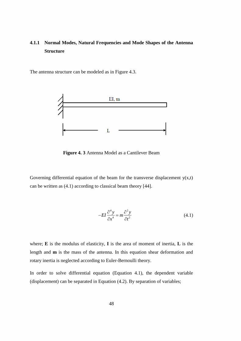
48
4.1.1 Normal Modes, Natural Frequencies and Mode Shapes of the Antenna
Structure
The antenna structure can be modeled as in Figure 4.3.
Figure 4. 3 Antenna Model as a Cantilever Beam
Governing differential equation of the beam for the transverse displacement y(x,t)
can be written as (4.1) according to classical beam theory [44].
4 2
4 2
y yEI m
x t
(4.1)
where; E is the modulus of elasticity, I is the area of moment of inertia, L is the
length and m is the mass of the antenna. In this equation shear deformation and
rotary inertia is neglected according to Euler-Bernoulli theory.
In order to solve differential equation (Equation 4.1), the dependent variable
(displacement) can be separated in Equation (4.2). By separation of variables;

49
( , ) ( ) ( )y x t Y x T t (4.2)
Letting a constant c to Equation (4.1) and separating both time and spatial
variables, differential equation of mode shapes can be written as in Equation (4.3).
4
2
4( ) ( ) 0
d mY x c Y x
dx EI
(4.3)
The solution to Equation (4.3) is the general form of transverse mode shapes of the
antenna structure.
General form of beam mode shapes can be presented as in (4.4)
1 2 3 4( ) sinh( ) cosh( ) sin( ) cos( )Y x a x a x a x a x (4.4)
Solving the differential Equation (4.3) with general form of Y(x) yields the total
displacement solution with respect to mode shapes.
4
1 2 3 4
2
1 2 3 4
sinh( ) cosh( ) sin( ) sinh( ) ...
sinh( ) cosh( ) sin( ) sinh( ) 0
a x a x a x a x
mc a x a x a x a x
EI
(4.5)
There is only one solution of Equation (4.5), which is presented in Equation (4.6).
4 2 m
cEI
(4.6)
In order to solve general differential equation of displacement solution presented in
Equation (4.5), boundary conditions of antenna structure should be determined.
From Equations (4.7) to (4.10) boundary conditions are presented.
The following boundary conditions can be specified for the antenna structure with
fixed base (x=0).

50
(0) 0Y (zero displacement condition) (4.7)
0 0x
dY
dx (zero slope condition) (4.8)
Following boundary conditions can be defined for antenna structure at the free end
where x=L.
2
20x L
d Y
dx (zero bending moment condition) (4.9)
3
030x
d Y
dx (zero shear force condition) (4.10)
These boundary condition can be applied to the general solution in Equation 4.5
and to its derivatives.
1
2
sin( ) sinh( ) cos( ) cosh( ) 0
cos( ) cosh( ) sin( ) sinh( ) 0
aL L L L
aL L L L
(4.11)
𝑎1 and 𝑎2 constants should be zero in order to satisfy Equation (4.11). Moreover,
the determinant should also be set to find a nontrivial solution. Therefore, the
solution is presented in Equation (4.12).
cos( ) cosh( ) 1n nL L (4.12)
Equation (4.12) can be defined as the frequency equation of cantilever beam [44].
It is a non-linear equation and the roots can be determined by means of a
combination of graphical and numerical methods. There exist an infinite number of
roots which represents the possible modes of vibration phenomena. Since the
system taken into consideration is a continuous system, there are infinite numbers
of natural frequencies. The roots of Equation (4.12) are displayed in Table 4.1 [44].

51
Table 4. 1 Values of nl for first Five Mode of Cantilever Beam [44]
n (modes) 𝜷𝒏𝑳
1 1.87510
2 4.69409
3 7.85409
4 10.99554
5 (2n-1)π/2
Using modal 𝛽𝑛 values, separated time equation can be written as follows [44].
2 2
1 2( ) sin sin 0n n
EI EIT t b t b t
m m
(4.13)
Therefore, the natural frequency of antenna structure 𝜔𝑛 can be defined as;
2
nn
EI
m (4.14)
For individual modes, 𝛽𝑛 values given in Table 4.1 are inserted into Equation
(4.14) in order to find corresponding natural frequency.
Finding natural frequencies of antenna structure, next step is to find eigenvectors.
For eigenvectors, general solution expressed by Equation (4.4) is recalled.
1 2 3 4( ) sinh( ) cosh( ) sin( ) cos( )Y x a x a x a x a x (4.15)

52
Eigenvectors can be found with directly applying boundary conditions (Equations
4.7-4.10) to Equation (4.4) and its derivatives. Eigenvector equation presented in
Equation (4.16) becomes as follows:
2
cosh( ) cos( )( ) cosh( ) cos( ) sinh( ) sin( )
sinh( ) sin( )
L LY x a x x x x
L L
(4.16)
For generalized modal eigenvectors in arbitrary scale, Equation (4.17) can be
written.
cosh( ) cos( )
( ) cosh( ) cos( ) sinh( ) sin( )sinh( ) sin( )
n nn n n n n
n n
L LY x a x x x x
L L
(4.17)
These eigenvectors can be mass-normalized as in Equation (4.18).
2
0
( ) 1
L
nmY x dx (4.18)
After mass-normalization, the leading coefficient of all modes becomes one. Thus,
mass-normalized eigenvectors can be written using 𝛽𝑛 values are taken from Table
4.1. In order to determine mode shapes of an antenna structure, mass and length
information is enough for non-dimensional eigenvectors. Mode shapes are viewed
basically the visual behavior of antenna structure at natural frequencies.
Graphically, mode shapes can be displayed by plotting corresponding eigenvector
equation with respect to antenna length.

53
4.1.2 Effective Modal Mass and Participation Factor for the Antenna
Structure
The effective modal mass is an important method for judging whether the mode is
significant or not. Modes with relatively high effective masses can be readily
excited by base excitation. Considering an antenna structure modeled as a
cantilever beam, there is infinite number of modes present. In order to perform
transient analysis of the antenna structure, for brevity, only limited number of
modes should be included through analysis.
“In order to determine how many modes should be included in the analysis, the
number should be high enough so that the total effective modal mass of the model
is at least 90% of the actual mass [45].”
The participation factor (𝛤) for cantilever beam with constant mass density can be
defined by Equation (4.19) [45]. It should be noted that 𝑌𝑛(𝑥) is the corresponding
mode shape. Therefore, participation factors are non-dimensional.
0
( )
L
n nm Y x dx (4.19)
Effective modal mass is, however, is a dimensional property. It is defined by the
vector which represents the displacement of the mass. For cantilever beams,
Equation (4.20) can be written for effective modal mass.
2
0
,2
0
( ) ( )
( ) ( )
L
n
eff n L
n
m x Y x dx
m
m x Y x dx
(4.20)

54
As given in Equation (4.18), eigenvectors, ( )nY x can be mass-normalized. In terms
of mass-normalized eigenvectors, Equation (4.21) can be written for effective
modal mass.
2
2
,
0
( ) ( )
L
eff n n nm m x Y x dx
(4.21)
4.1.3 Transient Response of the Antenna Structure to Base Excitation
Antenna model corresponding to the transient base excitation can be sketched as
Figure 4.4.
Figure 4. 4 Antenna Model Subjected to Transient Base Excitation
The forced transient response equation for a cantilever beam with beam excitation
is given in Equation (4.22) [46].

55
4 2 2
4 2 2
d y y wEI m m
dx t t
(4.22)
In Equation (4.22), y(x,t) is the relative displacement with respect to the base and
w(t) is the base displacement while the term on the right-hand-side is the inertial
force.
For the dependent variable y(x,t), Equation (4.23) is written.
1
( , ) ( ) ( )m
n n
n
y x t Y x T t
(4.23)
With the expansion of y(x,t), governing equation can be written in the form of
Equation (4.24).
4 2 2
4 2 21 1
r r
n n n n
n n
wEI Y x T t m Y x T t m
x t t
(4.24)
Equation (4.25) is obtained in terms of n values as:
2 2
4
2 21 1
r r
n n n n n
n n
d d wEI Y x T t m Y x T t m
dt dt
(4.25)
Each term is multiplied by an arbitrary mode shape function ( )pY x . Therefore
Equation (4.26) is written as;
2 2
4
2 21 1
r r
n n n n n
n n
p p p
d d wEI T t Y x Y x m Y x Y x T t m Y x
dt dt
(4.26)

56
In order to calculate the complete response of the antenna, integration is performed
over the antenna length.
4 2
21 10 0
2
2
0
L Lr r
p pn
n n
p
n n
n n
L
EI dT t mY x Y x dx T t mY x Y x dx
m dt
d wmY x dx
dt
(4.27)
Orthogonality of the eigenvectors ( )nY x and ( )pY x is exploited for simplifications
in Equation (4.27). Orthogonality conditions are presented in Equations (4.28) and
(4.29).
0
( ) ( ) 0
L
n pmY x Y x dx for n p (4.28)
0
( ) ( ) 1
L
n pmY x Y x dx for n=p (4.29)
Making use of Equations (4.18) and (4.24) and orthogonality properties,
differential equation (4.27) becomes a complete form presented in Equation (4.30).
2 22
2 2( ) ( )n n n n
d d wT t T t
dt dt (4.30)

57
Finally, damping term is included to the differential equation in the form of modal
damping ratio n .
2 22
2 2( ) 2 ( ) ( )n n n n n n n
d d d wT t T t T t
dt dt dt (4.31)
2( ) 2 ( ) ( ) ( )n n n n n n nT t T t T t w t (4.32)
Damped natural frequency can be defined by Equation (4.33), as
21d n (4.33)
The discrete form of Equation (4.32) is inefficient to solve even on a computer.
Therefore, time variable nT can be solved from a ramp invariant recursive filtering
relationship [21, 46]. The term recursive refers to the fact that the response at any
time depends in part on the responses at all previous times. The term filtering refers
to the fact that the system itself behaves as a simple low-pass filter. In fact, the time
integration process itself is a low pass filtering operation. The derivation of the
filtering relationship may be performed by an extensive number of steps in the time
domain. However, it is a very inefficient and time-consuming process. Therefore,
derivation of the coefficient of time variable is performed by frequency domain
transformation methods, particularly the series of Z-transform, Laplace Transform
and Inverse Laplace Transform methods.
Time variable nT is found via RFR method as presented in Equation (4.34), noting
that t is the time step.

58
, , 1 , 2
3 2
3
2exp cos cos exp 2 ...
2 exp( )cos( ) 1 exp( )...1
...2 1 sin( )
2 exp( )cos( ) 2 1 exp( 21
n i n d d n i n n i
n d n
n inn d n
d
n n d
n
T t t t T t T
t t t
wm t t t
t t t
m t
12
223
) ...
...2 2 1 exp( )sin( )
(2 )exp( 2 ) exp( )...1
2 1 sin( ) 2 cos( )
n
n inn d
d
n n n
n ind dn
d
t
wt t
t t t
wt tm t
(4.34)
Time variables nT and eigenvectors nY are sufficient enough to solve for antenna
relative displacement, relative velocity and relative acceleration.
Antenna relative displacement is given in Equation (4.35), where n is the mode
number.
1
( , ) ( ) ( )r
n n
n
y x t Y x T t
(4.35)
Antenna relative velocity is expressed in Equation (4.36).
1
( , ) ( ) ( )r
n n
n
y x t Y x T t
(4.36)
Antenna relative acceleration is expressed in Equation (4.37) through time
differentiation.
1
( , ) ( ) ( )r
n n
n
y x t Y x T t
(4.37)

59
Antenna absolute acceleration ( , )A x t can be found by summation of base
acceleration input and antenna relative acceleration as presented in Equation (4.38).
( , ) ( ) ( , )A x t w y y x t (4.38)
Solution Methods for Transient Response of the Antenna Structure
Subjected to Base Excitation
In this section, solution methods for transient response of the antenna structure
subjected to base excitation are presented. Solution methods are categorized,
namely, as multi-degree-of-freedom solutions, single-degree-of-freedom solutions
and approximate solutions.
The main purpose of this chapter is to derive the multi-degree-of-freedom transient
solution of antenna structure and develop the solution algorithm of the model
derived. Multi-degree-of-freedom solution methods of antenna structure are the
solution to the mathematical model presented in Section 4.2. Therefore, solution
methodology is focused specifically on recursive filtering relationship (RFR).
Recursive algorithm for this methodology uses the modal analysis results of
continuous modeling with classical theory presented in Sections 4.2.1 and 4.2.2.
The solution algorithm calculates the modal analysis results of antenna structure
and makes use of these results on transient response calculations. At the same time,
ramp invariant recursive filtering relationship employed used to solve the series of
equations presented in Section 4.2.3. Thus, a complete transient analysis of antenna
structure based on continuous modal analysis is achieved. For multi-degree-of-
freedom solution, exact transient solution of antenna structure subjected to the
classical pulse input can be calculated. Exact solution is also calculated in order to
compare algorithm solutions to the exact solution. RFR method can be applied to

60
various shock inputs, while the use of exact solution is limited only to the classical
pulse input (e.g. half-sine input).
Solution methods employing single-degree-of-freedom model are also presented in
this section. In this study, these methods are built before multi-degree-of-freedom
methods in order to foresee the behavior of antenna structure with the assumption
that the antenna structure possesses only one mode. Regard to the participation
factor of modes of MDOF structure, SDOF assumption may yield very close
estimation. For single-degree-of-freedom analysis, convolution integral solution,
RFR method, Runge-Kutta fourth order method and Newmark-beta numerical
integration methods are presented. Single-degree-of-freedom methods can be used
to monitor general shock response behavior of antenna structure to transient
impulse. For simple geometries, these methods can be used for shock analysis with
certain amount of errors. The source of these errors is the lumped mass assumption.
Lumped mass theory uses the natural frequency of the lumped mass of the system
and equivalent stiffness. Therefore, lumped mass results do not include
participations of all modes whose effective modal percentages are relatively high.
Thus, single-degree-of-freedom modeling with lumped mass theory presents
responses with certain amount of error. SDOF modeling results can also be used
for approximate response calculations. With the use of corresponding response
values for acceleration, displacement or velocity for each natural frequency,
approximate solutions can be obtained by simplified methods.
In this section, simplified methods are also presented. Simplified modal
combination methods are used to estimate the multi-degree-of-freedom response.
Estimations require only eigenvalues, eigenvectors and the modal participation
factors of the system. Therefore, modal analysis results are combined as the
summation of single-degree-of-freedom results for multi-degree-of-freedom
estimation. Due to their simplicity and speed, simplified methods can be used for
the modal analysis for simple structures to determine the general shock response
behavior of the system.

61
4.2.1 Multi-Degree-of-Freedom (MDOF) Solution Methods
4.2.1.1 Ramp Invariant Recursive Filtering Relationship Method
Transient response of antenna structure is obtained in Section 4.1, Recursive
Filtering Relationship (RFR) uses the ramp invariant technique which models the
slope between adjacent points of the input excitation. Modal analysis of the system
should have been performed before using the RFR technique and the system is
reduced to uncoupled mass, damping and stiffness matrices [47, 48]. The response
in physical coordinated can be obtained from the modal responses after the
transient analysis. Initial conditions are all kept at zero. Therefore, the response to
initial conditions can be solved exactly by using Laplace transforms, if preferred.
In the analysis, the time step should be selected so that there are at least ten points
per cycle corresponding to the highest natural frequency of interest. Therefore,
sample rate should be a least ten times the highest frequency of interest. As
Smallwood proposed in his paper [21], with the improved ramp invariant method,
the analysis can be performed at a sampling rate two times the highest frequency.
Still, to be safe side, at least ten times rule is recommended for the users. The
number of modes which are included the analysis can be determined by
participation factors of individual modes. As noted in Section 4.2.2, the number of
modes included should be high enough so that the total effective modal mass of the
model is at least 90% of the actual mass.
In order to obtain transient response of antenna structure, a MATLAB® code is
developed including the modal analysis with classical approach presented in
Sections 4.2.1 and 4.2.2. It also includes the solution algorithm with the solver of
the equations presented in Section 4.2.3. Solution algorithm behind the written
code is presented in Figure 4.5.

62
Figure 4. 5 Solution Methodology of MATLAB® Script Built for RFR Method
4.2.1.2 Other Numerical Methods
In order to solve antenna response model with numerical integration, there exist
some other frequently used numerical methods. Among these numerical integration
methods, Newmark-Beta time integration method, Backward-Euler method and
central difference method are implemented in various commercial finite element
programs for both linear and non-linear problems. Newton–Raphson method is also
among those standard techniques which are specified with large deflection
nonlinearities. The important parameters for these methods are selected time step,
convergence criterion, modal analysis integration to the algorithm, solution
accuracy and computational efficiency. Numerical methods are especially used for
Property Entry
•Geometrical and Material Properties are entered.
Boundary condition selection
•Boundary condition is selected for analysis.
Modal Analysis
•Natural frequencies, eigenvalues and eigenvectors are found and inputted to transient analysis
Shock inputs
•Acceleration input magnitude and profile is defined with duration of shock.
RFR Calculation
•Coefficients of RFR are calculated.
Recursive Calculation
•Responses are calculated recursively.
Postprocess
•Postprocessing is performed in order to present maximum values of responses and tto plot time-history responses.

63
nonlinear numerical integration which is very time consuming and computation
efficiency dependent process. The solution algorithms are based on spatial
discretization of the system with the governing equilibrium equation of structural
dynamics [51, 52].
4.2.2 Single-Degree-of-Freedom (SDOF) Solution Methods
For SDOF modeling of antenna structure, antenna structure should be represented
as a lumped mass model. Antenna stiffness can be calculated by Equation (4.39).
3
3beam
EIk
L (4.39)
Natural frequency of the beam with lumped mass assumption is presented in
Equation (4.40).
3
1 3
2n
EIf
mL (4.40)
Remaining part is the solution of the response equation of the SDOF system at its
natural frequency.
4.2.2.1 Convolution Integral Method
The convolution integral method yields an exact solution for the response only if
the system and the input pulse can be analyzed in analog form rather than digital
form. Therefore, this is impractical. The nested series representation of the
convolution integral is also not commonly used because it is numerically
inefficient. However, digital recursive filtering relationship representation of the

64
convolution integrals with discrete time domain gives the numerically practical
solution.
4.2.2.2 Digital Recursive Filtering Relationship Method
This method is previously introduced in Chapter 3 while shock response spectrum
is obtained. In this method, convolution integral is represented as digital recursive
filtering relationship. The derivation of the shock response equation is performed
using Z-transform. The ramp invariant simulation is preferred in this method since
better accuracy is achieved with the addition of a filtering term. As discussed in
MDOF use of this method, constant time step is used. The result of acceleration
shock response is already presented in Equation (3.7). Solutions of transient
response analysis are calculated via previously built MATLAB® code in Chapter
3. The outcome of this analysis is that, the ramp invariant digital recursive filtering
relationship found for this calculation is used as the starting point of the numerical
engine of MDOF modal transient analysis presented in Sections 4.2.3 and 4.3.1 for
respective response parameters.
4.2.2.3 Newmark-Beta Method
The Newmark-Beta method is performed for a variable time step for the input. It
can be used for the direct integration of a system of uncoupled mass, damping, and
stiffness matrices. It can be applied to an uncoupled system as well. This method is
derived from the continuous time equation in a general form as presented in
Equation (4.39) [50, 51]. In order to compare SDOF solution techniques,
MATLAB® code for this method is prepared for the transient response analysis.

65
4.2.2.4 Runge-Kutta 4th Order Method
The Runge-Kutta method extends the Taylor series method by estimating higher
order derivatives at points within the time step. Among the methods built on
Runge-Kutta method, Runge-Kutta 4th Order Method is preferred for arbitrary input
function. [46]. Again, in order to compare SDOF solutions exerted from different
techniques, MATLAB® code is prepared for transient response analysis via
Runge-Kutta 4th Order Method.
4.2.3 Simplified Solution Models
In some cases, MDOF solution of antenna structure may be too difficult to handle
with complete model and SDOF solution may contain unacceptable amount of
error. Simplified solution methods can offer the best solution for such cases.
Simplified methods use the SDOF responses of each modal response separately of
antenna structure and sum those modal responses by different methods. These
methods cannot present the faithful responses as MDOF models but it presents far
better approximates than the SDOF models in most cases.
4.2.3.1 Absolute Sum Method (ABSSUM)
The absolute sum presents a conservative approach since this method is based on
the assumption that the maxima of all modes can be observed at the same instant of
time, i.e. with no phase difference. Maximum relative displacement max( )iz can be
calculated from modal coordinates. Equation (4.42) is used for the estimation for

66
this method. Noting that ˆnjq is the corresponding eigenvalue. Absolute acceleration
can also be found by the same formulation.
max ,max
1
ˆ( )r
n j nj j
j
z q z
(4.41)
4.2.3.2 Square Root of the Sum of the Squares (SRSS)
This method approximates the relative displacement of MDOF system with the
square roots of the squares of the summation values for modal maximum relative
displacements. The estimated relative displacement is presented in Equation (4.43).
Absolute acceleration is also found by the same formulation.
2
max ,max
1
ˆ( )r
n j nj j
j
z q z
(4.42)
4.2.3.3 Naval Research Laboratories Method (NRLM)
“NRL method is a statistical estimate of the maximum response created by taking
the response for the mode that exhibits the largest response. [54]” The maximum
relative displacement value is calculated from modal coordinates as presented in
Equation (4.44). For absolute acceleration the same procedure is applied.
max max max
1,
ˆ ˆ( ) ( )( ) ( )( )r
n nj n n nk k k
k k j
z q z q z
(4.43)

67
In this chapter, mathematical model of the antenna structure is presented, and
solution alternatives of these models are proposed. In this study, distributed
parameter modeling of the antenna with classical theory and MDOF modeling and
transient response solution of the antenna structure by RFR method are applied to
simulate shock response of antenna structure subjected to underwater explosions as
close as possible. For completeness, SDOF models are also presented with different
solution alternatives in order to foresee the response characteristics of antenna
structure. In addition to that, simplified methods are also presented for shock
analysis. With these methods, shock response of structures whose effective modal
masses of leading modes are high can be approximated better than SDOF
approximations.

68

69
CHAPTER 5
5TRANSIENT RESPONSE ANALYSIS OF ANTENNA
STRUCTURE
Mathematical model of the antenna structure is built on the basis of modal analysis
by means of continuous modeling with classical approach (Euler-Bernoulli Beam
Theory) and MDOF modal transient analysis with RFR method which is presented
in Chapter 4. Apart from that model, SDOF transient model and simplified models
are also presented for completeness. In this chapter, transient response analysis is
performed by these models. Following the roadmap of analysis procedure, first,
MDOF transient response analysis which is the main purpose of the study is
performed by RFR method. Modal analysis outputs such as natural frequencies,
mode shapes and participation factors are used as inputs for RFR transient analysis.
Therefore, this analysis can also be called as Modal Transient Analysis because of
the use of modal matrices built in continuous modeling. Shock profiles simulating
underwater explosions obtained in Chapter 3 are also used as acceleration inputs.
The output of analysis includes displacement, acceleration and velocity shock
responses obtained at any point on the antenna structure. Critical displacement and
acceleration response ranges are investigated with Phase Portrait plots. Histograms
also present the reluctance of antenna structure to failure or electromagnetic
malfunctions.
Secondly, simplified methods are presented involving three different methods
presented in Chapter 4. Maximum absolute acceleration and relative displacements
are estimated by means of these methods. A comparative evaluation of results is
carried to understand the efficiency of these simplified models in predicting the
antenna response to shock input as described. Finally SDOF transient analysis is
presented. For SDOF transient analysis, three different methods are used. Results

70
of these methods are compared between each other and compared with MDOF
results. Since SDOF transient analysis methods are based on very primitive and
geometry-independent model, it is expected that responses are not very close to
MDOF models naturally. For all analysis procedures, MATLAB® scripts are built
and results are obtained by means of these scripts.
Modal Analysis of Antenna Structure
Antenna structure and base platform mentioned in Chapter 4 is sketched in Figure
5.1. Important geometric parameters are labeled on the figure. Numerical values of
these parameters are presented in Table 5.1. These dimensions are determined by
electromagnetic design of the antenna structure.
Figure 5. 1 Three-Dimensional Model of Antenna Structure
Table 5. 1 Geometrical Properties of Antenna Structure
Geometrical Properties
Antenna length (mm) 370
Antenna width (mm) 20
Antenna thickness (mm) 2

71
Generally 5000 or 6000 series of aluminum alloys are used for antenna structures
due to the strength, corrosion, weight, machining and electrical conductivity
concerns. AA6061-T6 material is used for the dipole antenna considered in this
thesis. Mechanical properties of AA6061-T6 are presented in Table 5.2.
Table 5. 2 Mechanical Properties of Antenna Structure
Mechanical Properties of AA6061-T6
Young Modulus (GPa) 68.9
Density (kg/m3) 2768
Poisson’s Ratio 0.33
Modal Analysis of antenna structure is performed via MATLAB® code written.
Geometric properties and material properties of antenna structure are introduced to
the code as input parameters which are tabulated as in Table 5.1 and 5.2. Using
Table 4.1, Equations (4.14) and (4.17); natural frequencies and mode shapes are
calculated. Results are presented in Table 5.3 and Figure respectively. Noting that
number of modes included into the transient analysis should be determined before
the analysis. After certain amount of modal mass percentage of degree-of-
freedoms, transient response of the antenna does not change significantly.
Procedure for the selection of number of modes to be included to the transient
analysis is explained in Section 5.2 briefly.
Table 5. 3 Natural Frequencies of Antenna Structure for First Four Bending Modes
Natural Frequencies of Antenna Structure
First Mode Natural Frequency (Hz) 11.78
Second Mode Natural Frequency (Hz) 73.79
Third Mode Natural Frequency (Hz) 206.62
Fourth Mode Natural Frequency (Hz) 404.90

72
Figure 5. 2 First Four Bending Mode Shapes of Antenna Structure
MDOF Transient Response Analysis of Antenna Structure
5.2.1 Determination of Analysis Parameters
Electromagnetic point of view requires that the antenna structure should be
maintained perpendicularly with respect to its base ground. In other words, the
antenna structure should be avoided from excessive amount of bending and
electronic components placed in vicinity of antenna tip should be in the same
longitudinal direction with the antenna base where the power to the antenna is
supplied. Antenna performance is directly proportional to the straightness of
aluminum beam in longitudinal direction. This means transverse shock inputs to
the antenna structure are very critical, because such lateral shock inputs subject the
beam with bending. However, shock inputs in vertical direction which is acting on
the antenna longitudinal axis, only create the longitudinal motion of antenna with
0 0.05 0.1 0.15 0.2 0.25 0.3 0.35 0.4-1
-0.8
-0.6
-0.4
-0.2
0
0.2
0.4
0.6
0.8
1
Mo
de S
hap
e A
mp
litu
de
Antenna Span
Mode Shapes of Antenna with Length=0.37m, Width=0.02m, Thickness=0.002m
First Mode
Second Mode
Third Mode
Fourth Mode

73
the base. Therefore longitudinal distance between antenna structure and the other
antennas used in the system does not change and bending motion of antenna
structure is not observed. This implies that there is no change in antenna
performance individually and no change in system performance due to such
loading. In addition to that, from stress standpoint, maximum stress values for these
three inputs are investigated and maximum stress for transverse loading is observed
as higher than maximum stress obtained from vertical loading due to buckling.
Thus, maximum stress is observed at the face near to the antenna base due to the
bending motion caused by transverse loading.
Considering the shock inputs synthesized and tabulated in Table 3.4, transverse and
longitudinal shock inputs to the base can create bending motion to the antenna
structure with regards to the placement of antenna. However, vertical shock input
to the base does not create bending motion as illustrated in Figure 5.3.
Figure 5. 3 Shock Inputs Applied to the Antenna Platform

74
As seen in Figure 5.3, transverse and longitudinal shock inputs should be
considered for this study. Transverse and longitudinal inputs are considered
together, because regarding to the antenna attachment to the platform, these two
axes can be interchanged. Therefore, both inputs are the candidates of bending
motion of antenna structure and may severe the electrical components or trigger
antenna structure failure. In order to compare the effect of both transverse shock
inputs SRS curves of the acceleration shock inputs (100g 8ms half-sine and 200g
8ms half-sine) are plotted together. As the acceleration response is important for
component and material failure and the relative displacement response is important
for antenna performance, both graphs are plotted and examined in Figure 5.4 and
Figure 5.5.
Figure 5. 4 Acceleration SRS for both Transverse Shock Inputs
100
101
102
103
104
105
100
101
102
103
Peak A
ccele
ration (
G)
Natural Frequency (Hz)
Acceleration Shock Response Spectrum
100g 8ms half-sine
200g 8ms half-sine

75
Figure 5. 5 Relative Displacement SRS for both Transverse Shock Inputs
As shown in Figure 5.4 and 5.5, 200g 8ms half-sine shock input includes the
response levels of 100g 8ms shock input. Therefore it is logical to perform the
analysis with 200g 8ms half-sine shock input to be on the safe side.
After the shock input is determined, number of modes to be included in transient
analysis is determined. “In order to determine how many modes should be included
in the analysis, the number should be high enough so that the total effective modal
mass of the model is at least 90% of the actual mass [45].” Therefore, effective
modal masses of first 8 modes are calculated and tabulated in Table 5.4.
100
101
102
103
104
105
10-8
10-6
10-4
10-2
100
102
Rela
tive D
ispla
cem
ent
(m
m)
Natural Frequency (Hz)
Relative Displacement Shock Response Spectrum
100g 8ms half-sine
200g 8ms half-sine

76
Table 5. 4 Modal Properties of the Antenna Structure
Mode
Natural
Frequency
(Hz)
Participation
Factor
Effective
Modal Mass
(kg)
Modal Mass
Percentage
(%)
1 11.78 0.1585 0.0251 61.22
2 73.79 0.0878 0.0077 18.78
3 206.62 0.0515 0.0027 6.59
4 404.90 0.0368 0.0014 3.41
5 669.33 0.0286 0.0008 1.95
6 999.86 0.0234 0.0005 1.22
7 1396.50 0.0198 0.0004 0.98
8 1896.24 0.0172 0.0003 0.49
From results given in Table 5.4, first four modes are sufficient to include the
analysis since the total effective modal mass percentage of first four modes is 90%.
Comparison of transient responses of the antenna structure with respect to the
number of modes included to the analysis is presented in Figures 5.6-5.9. As
concluded from these graphs, after two modes results are changing in an interval of
0.04%. Therefore, it is concluded that 4-mode analysis suffices to obtain acceptably
accurate results from MDOF transient analysis by RFR Method.

77
Figure 5. 6 Comparison of transient acceleration responses of antenna structure
with respect to the number of modes included in the analysis
Figure 5. 7 Comparison of transient acceleration responses of antenna structure
with respect to the number of modes included in the analysis (Zoomed View)
0 0.05 0.1 0.15 0.2 0.25 0.3 0.35 0.4-300
-200
-100
0
100
200
300
400
Ab
so
lute
Accele
rati
on
(G
)
Time (sec)
Acceleration Response of Antenna
1-mode
2-mode
3-mode
4-mode
5-mode
6-mode
0.01 0.02 0.03 0.04 0.05 0.06 0.07-300
-200
-100
0
100
200
300
Ab
so
lute
Accele
rati
on
(G
)
Time (sec)
Acceleration Response of Antenna
1-mode
2-mode
3-mode
4-mode
5-mode
6-mode

78
Figure 5. 8 Comparison of relative displacement responses of antenna structure
with respect to the number of modes included in the analysis
Figure 5. 9 Comparison of relative displacement responses of antenna structure
with respect to the number of modes included in the analysis (Zoomed View)
0.01 0.02 0.03 0.04 0.05 0.06 0.07 0.08
-0.2
-0.15
-0.1
-0.05
0
0.05
0.1
0.15
Rela
tive D
isp
lacem
en
t (m
)
Time (sec)
Relative Displacement Response of Antenna
1-mode
2-mode
3-mode
4-mode
5-mode
6-mode

79
5.2.2 MDOF Transient Response Analysis Results
MDOF transient response analysis of antenna structure is performed for 200g 8ms
half-sine acceleration shock input to the antenna base, including 4 modes of
antenna structure. Outputs are measured from the antenna tip where electrical
components are placed and the antenna structure has maximum deformation
nearby. As outputs, absolute acceleration is designated in order to monitor the
effect of shock explosion to the antenna structure. Results are expressed in
gravitational acceleration “g”. Acceleration output is the best determinate for
damage potential and severity of underwater explosions on antenna structure.
Endurance of electrical components and fatigue concerns are determined from
acceleration output. As another output, relative displacement of the antenna tip is
measured. Maximum deflection is monitored at the antenna tip, therefore the
antenna performance is directly proportional to the deflection amplitude of the
structure. Thus, relative displacement is another important output of the transient
analysis. As an additional study, relative velocity of antenna tip is considered.
From relative velocity response, stress value at antenna tip can be estimated. This is
an estimation process because since shock pulses are applied to the structure for
very small interval of time, stresses obtained from the analysis are called “pseudo
stress”. Therefore, correction of those stresses will be performed and strength
calculations of beam structure and electrical components will be calculated.
Relative velocity outputs are presented in this section and stress calculation is
performed and discussed in Chapter 8.
For the analysis procedure, formulations presented in Sections 4.1 and 4.2.1 are
used and calculations are performed via MATLAB® script built for the complete
MDOF transient response analysis using RFR Method. In MATLAB® script,
procedure presented in Figure 4.5 is followed. Modal damping ratio is taken as
0.05 for all four modes [23].

80
A 200g 8ms half-sine acceleration shock input presented in Figure 5.10 is adopted
as the input in the analysis.
Figure 5. 10 Time History of 200g 8ms Half-Sine Acceleration Input
Absolute acceleration response of the antenna tip to the shock 200g 8ms shock
input is illustrated in Figure 5.11. Peak value of response is measured as 310.6 g.
0 0.005 0.01 0.015 0.02 0.025 0.030
20
40
60
80
100
120
140
160
180
200
220
Time (sec)
Accele
rati
on
(G
)
Time History of Acceleration Input
200g 8ms half-sine

81
Figure 5. 11 MDOF Absolute Acceleration Response of the Antenna Tip
Relative displacement response of antenna structure is shown in Figure 5.12. For
relative displacement, maximum value is measured as 0.199 mm.
0 0.05 0.1 0.15 0.2 0.25 0.3 0.35 0.4-300
-200
-100
0
100
200
300
400Acceleration Response of Antenna Tip
Accele
rati
on
(G
)
Time (sec)
Acceleration Response
200g 8ms Half-sine Input

82
Figure 5. 12 MDOF Relative Displacement Response of the Antenna Tip
Relative velocity response of the antenna tip is displayed in Figure 5.13. Maximum
velocity at the tip point is measured as 18.58 m/s.
0 0.05 0.1 0.15 0.2 0.25 0.3 0.35 0.4
-0.2
-0.15
-0.1
-0.05
0
0.05
0.1
0.15
0.2R
ela
tiiv
e D
isp
lacem
en
t (m
)
Relative Displacement Response of Antenna Tip
Time (sec)
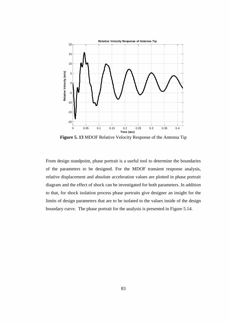
83
Figure 5. 13 MDOF Relative Velocity Response of the Antenna Tip
From design standpoint, phase portrait is a useful tool to determine the boundaries
of the parameters to be designed. For the MDOF transient response analysis,
relative displacement and absolute acceleration values are plotted in phase portrait
diagram and the effect of shock can be investigated for both parameters. In addition
to that, for shock isolation process phase portraits give designer an insight for the
limits of design parameters that are to be isolated to the values inside of the design
boundary curve. The phase portrait for the analysis is presented in Figure 5.14.
0 0.05 0.1 0.15 0.2 0.25 0.3 0.35 0.4
-20
-15
-10
-5
0
5
10
15
20
Rela
tive V
elo
cit
y (
m/s
)
Relative Velocity Response of Antenna Tip
Time (sec)

84
Figure 5. 14 MDOF Phase Portrait of the Antenna Tip
The distribution of absolute acceleration and relative displacement responses of the
antenna tip can be monitored by means of histogram diagrams. In order to plot
histogram diagrams for responses, 1719 total response points are taken. The
distribution of responses is presented out of 1719 possible response points.
Histogram plots are shown in Figures 5.15 and 5.16.
-0.2 -0.15 -0.1 -0.05 0 0.05 0.1 0.15 0.2-300
-200
-100
0
100
200
300
400
Accele
rati
on
(G
)
Relative Displacement (m)
Phase Portrait

85
Figure 5. 15 Histogram Plot for MDOF Absolute Acceleration Response
Figure 5. 16 Histogram Plot for MDOF Relative Displacement Response
-300 -200 -100 0 100 200 300 4000
100
200
300
400
500
600
700 Histogram
Co
un
ts
Acceleration (G)
-0.2 -0.15 -0.1 -0.05 0 0.05 0.1 0.15 0.20
50
100
150
200
250
300 Histogram
Co
un
ts
Relative Displacement (m)

86
MDOF transient response analysis of the antenna structure subjected to 200g 8ms
half-sine shock input is performed by RFR Method. In order to conduct further
studies like component endurance, shock isolation, stress analysis and component
fatigue absolute acceleration, relative displacement and relative velocity time
histories are concerned. Furthermore, phase portrait and histogram plots are also
presented in order to find out the allowable region for shock design procedures.
Maximum response values found by MDOF analysis through RFR Method is
tabulated in Table 5.5.
Table 5. 5 Maximum Shock Responses at the Antenna Tip
MDOF Maximum Transient Responses
Absolute Acceleration (G) 310.6
Relative Displacement (m) 0.199
Relative Velocity (m/s) 18.58
Transient Analysis Results of Antenna Structure by Simplified Methods
In this section, transient analysis results of the antenna structure are presented by
three different methods mentioned in section 4.2.3. These simplified methods are
proposed for estimating the MDOF response. For analysis, eigenvalues,
eigenvectors and modal participation factors of the system or estimates of those are
required along with SRS values of corresponding natural frequencies. Since
simplified methods provide maximum values of responses, results obtained from
these methods are compared to maximum values of MDOF modal transient
analysis performed in Section 5.2.

87
5.3.1 Transient Response Results of ABSSUM Method
ABSSUM equation is again given in Equation (5.1).
max ,max
1
ˆ( )r
n j nj j
j
z q z
(5.1)
Equation (5.1) can be solved using, eigenvalues and participation factors taken
from MDOF modal transient analysis in Section 5.2. Relative displacement and
acceleration values are acquired from SRS analysis to 200g 8ms half-sine
acceleration input. The procedure is performed by means of MATLAB® script.
Results are tabulated in Table 5.6.
Table 5. 6 Transient Response Estimations of the Antenna Using ABSSUM
Method
Response
Modal Transient
Results (MDOF
RFR Method)
ABSSUM Method
Absolute
Acceleration
(G)
310.6 380.7
Relative
Displacement
(m)
0.199 0.212

88
5.3.2 Transient Response Results of SRSS Method
SRSS equation is again given in Equation (5.2).
2
max ,max
1
ˆ( )r
n j nj j
j
z q z
(5.2)
Equation (5.2) can also be solved with same inputs explained in Section 5.3.1. The
procedure is performed by means of a MATLAB® code written. Results are
tabulated in Table 5.7.
Table 5. 7 Transient Response Estimations of the Antenna Using SRSS Method
Response
Modal Transient
Results (MDOF
RFR Method)
ABSSUM Method
Absolute
Acceleration
(G)
310.6 292.8
Relative
Displacement
(m)
0.199 0.199
5.3.3 Transient Response Results of NRL Method
NRL equation is again given in Equation (5.3).
max max max
1,
ˆ ˆ( ) ( )( ) ( )( )r
n nj n n nk k k
k k j
z q z q z
(5.3)

89
Table 5. 8 Transient Response Estimations of the Antenna Using NRL Method
Response
Modal Transient
Results (MDOF
RFR Method)
ABSSUM Method
Absolute
Acceleration
(G)
376.6 292.8
Relative
Displacement
(m)
0.211 0.199
Simplified methods use the superposition of the mode shapes and SRS responses of
corresponding natural frequencies with the weight of participation factor. For
ABSSUM method, absolute response values of the number of selected modes are
superposed together. Therefore, the response is expected to be the highest than the
exact response or MDOF modal transient analysis response. Thus it can be
concluded that ABSSUM method provides the maximum possible response value
of the structure considered, and designs should be made assuming the exact
response is lower than the response obtained from this method. Therefore,
ABSSUM method can be used for determining the maximum response limit of
antenna structure. Inherently, SRSS and NRL methods are expected to yield closer
estimates of antenna structure. For NRL method, two-mode analysis produces the
same result with the ABSSUM method because formulations become the same for
this case. SRSS method is observed as the better estimate using considerably lower
number of modes. Considering two-mode and three-mode analysis, SRSS results
are the best estimated. Response values are tabulated for those three methods using
two and three modes in Table 5.9 and 5.10. Comparing both cases, two-mode
analysis is to be selected for future analysis since estimates are closer for this case
as proposed in literature [53].
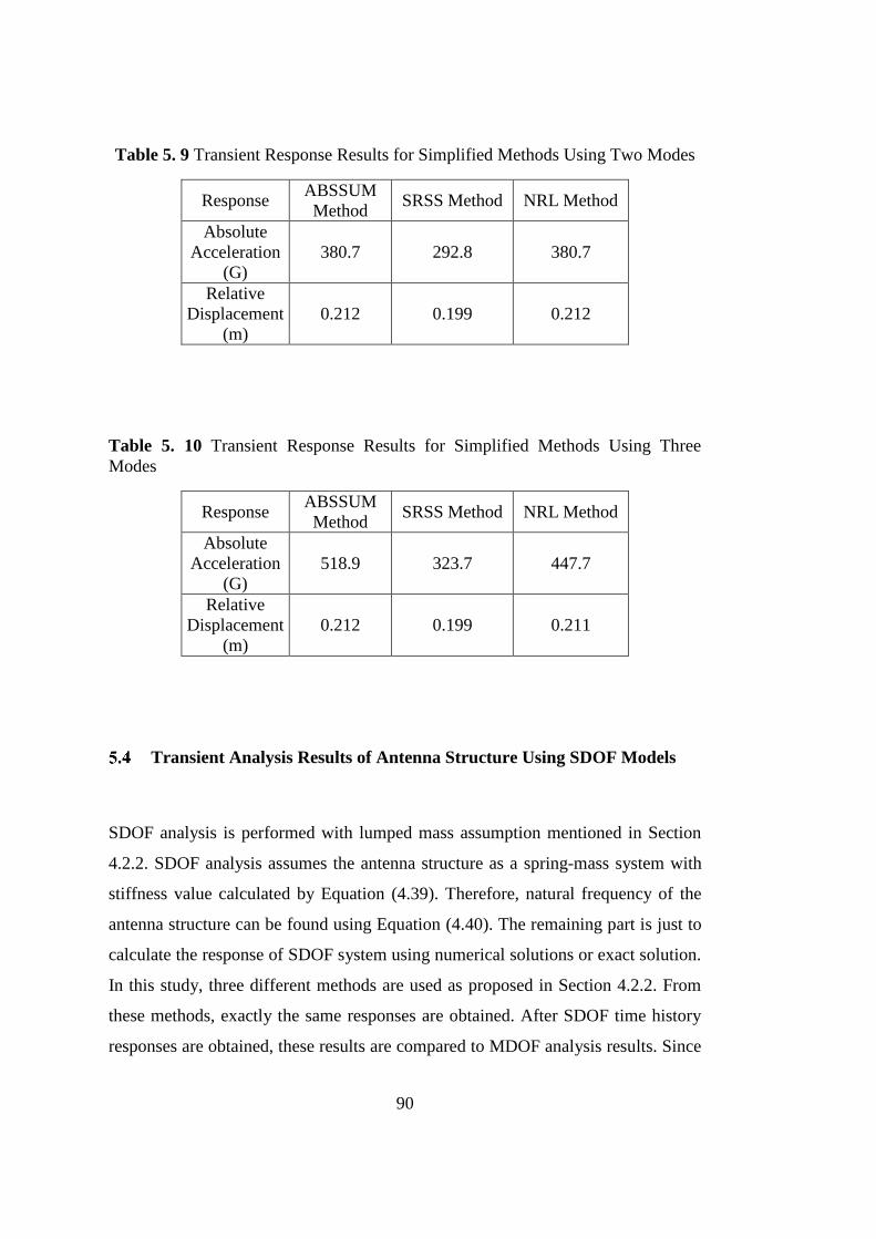
90
Table 5. 9 Transient Response Results for Simplified Methods Using Two Modes
Response ABSSUM
Method SRSS Method NRL Method
Absolute
Acceleration
(G)
380.7 292.8 380.7
Relative
Displacement
(m)
0.212 0.199 0.212
Table 5. 10 Transient Response Results for Simplified Methods Using Three
Modes
Response ABSSUM
Method SRSS Method NRL Method
Absolute
Acceleration
(G)
518.9 323.7 447.7
Relative
Displacement
(m)
0.212 0.199 0.211
Transient Analysis Results of Antenna Structure Using SDOF Models
SDOF analysis is performed with lumped mass assumption mentioned in Section
4.2.2. SDOF analysis assumes the antenna structure as a spring-mass system with
stiffness value calculated by Equation (4.39). Therefore, natural frequency of the
antenna structure can be found using Equation (4.40). The remaining part is just to
calculate the response of SDOF system using numerical solutions or exact solution.
In this study, three different methods are used as proposed in Section 4.2.2. From
these methods, exactly the same responses are obtained. After SDOF time history
responses are obtained, these results are compared to MDOF analysis results. Since

91
SDOF is very simple and does not contain any dependency on geometry of the
antenna structure and other modal properties, the results are far erroneous for
SDOF analysis especially for acceleration response as expected. For relative
displacement response, errors are more than simplified methods and results are not
close to MDOF model built in this thesis study. SDOF models are used for
simplified models mentioned in Sections 4.2.3 and 5.3 and shock profile synthesis
in Chapter 3. Moreover, SDOF DRFR method is used as a starting point for MDOF
RFR method development.
SDOF transient analysis responses are tabulated in Table 5.11 and plots are
presented in Figures 5.17-5.20.
Table 5. 11 SDOF Shock Responses at the Antenna Tip
SDOF Transient Responses
Absolute Acceleration (G) 69.52
Relative Displacement (m) 0.124
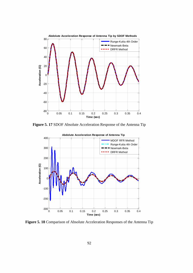
92
Figure 5. 17 SDOF Absolute Acceleration Response of the Antenna Tip
Figure 5. 18 Comparison of Absolute Acceleration Responses of the Antenna Tip
0 0.05 0.1 0.15 0.2 0.25 0.3 0.35 0.4-80
-60
-40
-20
0
20
40
60
80
Time (sec)
Accele
rati
on
(G
)
Abdolute Acceleration Response of Antenna Tip by SDOF Methods
Runge-Kutta 4th Order
Newmark-Beta
DRFR Method
0 0.05 0.1 0.15 0.2 0.25 0.3 0.35 0.4-300
-200
-100
0
100
200
300
400
Time (sec)
Accele
rati
on
(G
)
Abdolute Acceleration Response of Antenna Tip
MDOF RFR Method
Runge-Kutta 4th Order
Newmark-Beta
DRFR Method

93
Figure 5. 19 SDOF Relative Displacement Response of the Antenna Tip
Figure 5. 20 Comparison of Relative Displacement Responses of the Antenna Tip
0 0.05 0.1 0.15 0.2 0.25 0.3 0.35 0.4-0.2
-0.15
-0.1
-0.05
0
0.05
0.1
0.15
Time (sec)
Rela
tive D
isp
lacem
en
t (m
)
Relative Displacement Response of Antenna Tip by SDOF Methods
Runge-Kutta 4th Order
Newmark-Beta
DRFR Method
0 0.05 0.1 0.15 0.2 0.25 0.3 0.35 0.4
-0.2
-0.15
-0.1
-0.05
0
0.05
0.1
0.15
0.2
Time (sec)
Rela
tive D
isp
lacem
en
t (m
)
Relative Displacement Response of Antenna Tip
MDOF RFR Method
Runge-Kutta 4th Order
Newmark-Beta
DRFR Method

94
Phase portrait plot is also another tool to observe the region of SDOF analysis
responses in the MDOF transient response analysis. The participation of one mode
for transient responses can be clearly monitored in MDOF analysis, hence the
importance and contribution of other modes are observed. Thus, the necessity of
including at least more than one mode to the transient analysis is concluded.
Figure 5. 21 Comparison of Phase Portraits of the Antenna Tip
-0.2 -0.15 -0.1 -0.05 0 0.05 0.1 0.15 0.2-300
-200
-100
0
100
200
300
400
Relative Displacement (m)
Accele
rati
on
(G
)
Phase Portrait of Antenna Tip
MDOF RFR Method
SDOF RFR Method

95
Comments of Chapter 5
Results of mathematical modelling are presented in Table 5.12 along with exact
solution.
Table 5. 12 Mathematical Model Responses at the Antenna Tip
Maximum
Response
Exact
Result
MDOF
RFR
Method/
Error (%)
ABSSUM
Method/
Error (%)
SRSS
Method/
Error
(%)
NRL
Method/
Error (%)
SDOF
Model/
Error (%)
Absolute
Acceleration
(G)
310.5 310.6 /
0.03%
380.7/
22.6%
292.8/
-5.7%
380.7/
22.6%
69.5/
100%
Relative
Displacemen
t (m)
0.199 0.199 / 0% 0.212/
6.5%
0.199/
0%
0.212/
6.6%
0.124/
-37.7%
Comparing the results, MDOF modeling of antenna structure by RFR Method is
very satisfactory so as to present almost exact results. Therefore, validation of
MDOF mathematical model is achieved. This is very important to perform further
analysis studies for isolation, component fatigue and so on.
Exact solution is obtained from the toolbox by Yang [32] since the excitation is
classical pulse, antenna geometry can be modeled as a cantilever beam with initial
conditions all kept zero. However, for different types of excitation, for different
boundary conditions, it is not possible to find an exact solution. On the other hand,
MATLAB® script written for MDOF RFR Analysis is capable to perform analysis
with various shock inputs (e.g. square, sine, saw-tooth) and boundary conditions
like fixed-fixed or simply supported. Arbitrary shock inputs can even be analyzed
by MATLAB® script with some modifications on sampling and discretization.
Simplified methods estimates the transient response of antenna structure with
mode-superposition method. Doing this, modal information of antenna structure

96
and corresponding SRS value of mode interested is used. Therefore, it is better
approximation than SDOF analysis. For relative displacement, simplified methods
yields very closer results to MDOF analysis while the acceleration response
contains certain amount of error. Among these methods, SRSS method gives
acceptable results for antenna structure. Therefore, this method can be used as an
alternative for further studies like isolation and component fatigue. Other two
methods are more successful while differences between natural frequencies are
higher. NRL method, for example is the basis of Direct Dynamic Analysis Method
(DDAM). For this method, different methodology is followed for modal analysis
[55].
Single-degree-of–freedom solution is the most erroneous model among these
models because it is independent from geometrical and modal properties of
structure considered. In this study, SDOF model is utilized for determination of
SRS and building the MDOF model from SDOF basics of RFR Method.

97
CHAPTER 6
6TRANSIENT RESPONSE ANALYSIS OF ANTENNA
STRUCTURE BY FINITE ELEMENT ANALYSIS
In this chapter, transient response analysis of antenna structure subjected to
underwater shock explosions is performed by means of Finite Element Analysis
(FEA). In the scope of this chapter, modal and transient analyses are performed by
means of finite element software package ANSYS® R15.0. Antenna geometry
created on computer aided drawing software program (NX) is imported to
ANSYS® Workbench. Material properties of AA6061-T6 are introduced to the
engineering data library. Workbench-Modal and Transient commands are
employed for complete analysis along with Enforced Motion Extension. APDL
code is also written to introduce boundary conditions, shock inputs, base
acceleration input case and shock duration determination and obtain meaningful
shock outputs needed like absolute acceleration, relative displacement and relative
velocity. Modal analysis is performed to validate the antenna FEA model with
MDOF mathematical model results. Then, transient analysis follows with validated
model and shock responses are compared to MDOF model results. As an outcome
of this study, FEA modeling option is to be proposed as an alternative to
mathematical model in order to perform shock analysis from simple to complex
antenna structures.

98
Modal Analysis of Antenna Structure
ANSYS® Workbench 15.0 is used to perform modal analysis. From workbench
selections, “Modal (ANSYS)” is selected and dragged from Workbench to the
standalone project created. First, geometry should be created on Design Modeler in
ANSYS® Workbench or on any computer aided drawing software and then
imported to “Modal”. In the analysis, antenna geometry is imported to ANSYS® as
a pre-designed part file created by means of NX® 8.0. Since NX® 8.0 and
ANSYS® 15.0 are working interactively, it is the best and easiest way to create and
update models to be analyzed on ANSYS® platform. As the antenna material,
AA6061-T6 mechanical properties are imported to “Engineering Data Sources” of
ANSYS®. Properties are introduced with the values tabulated in Table 5.2. After
geometrical and mechanical properties are introduced, modal analysis properties
are defined one by one. Boundary conditions are introduced as a fixed support at
one end of antenna structure and free otherwise, and all initial conditions are
defined as zero. Meshing is defined with normal element sizes since structure is not
complex and it does not have irregular surfaces. As an output, total deformations
are selected and assigned for first five modes. From these assignments, natural
frequencies and mode shapes of corresponding modes can be monitored. After
modal analysis is performed, mode shapes and numerical results of natural
frequencies for bending modes are obtained. Mode shapes obtained from FEA are
presented in Figures 6.1 to 6.4.

99
Figure 6. 1 First Mode Shape of the Antenna Structure (FEA Result)
Figure 6. 2 Second Mode Shape of the Antenna Structure (FEA Result)

100
Figure 6. 3 Third Mode Shape of the Antenna Structure (FEA Result)
Figure 6. 4 Fourth Mode Shape of the Antenna Structure (FEA Result)
Comparing the mode shapes with mathematical model results presented in Figure
5.2, the mode shapes obtained from FEA model display expected shapes from
theoretical background. Natural frequencies are also obtained from FEA modal
analysis for the first four bending mode. It should be noted that in the ANSYS®
results, the third mode is not a bending mode. So the third mode is skipped and the
fourth mode reported by ANSYS® is taken as the third bending mode. Therefore,
first, second, fourth and fifth modes predicted by ANSYS® are the first four
bending modes of antenna structure. The reason behind this is that ANSYS®
analysis formulation used is based on Timoshenko beam theory which includes

101
shear-deformation effects and this effect is neglected in the Euler-Bernoulli beam
theory. First four bending modes presented by ANSYS® is tabulated in Table 6.1
and compared with mathematical model results obtained in Section 5.1.
Table 6. 1 Natural Frequencies of the Antenna Structure
Modes
Mathematical
Model
Results (Hz)
ANSYS®
Results (Hz)
Percentage
Difference of
FEA Results
1 11.78 11.89 0.93 %
2 73.79 74.75 1.30 %
3 206.62 208.67 0.99 %
4 404.90 409.33 1.09 %
ANSYS® results and theoretical results are not different more than 1.3% for the
first four modes. Thus the ANSYS® results match quite well with Euler-Bernoulli
beam theory. Transient analysis can be performed since model is validated.
Transient Response Analysis of Antenna Structure
Transient analysis is performed by means of ANSYS® Workbench. Transient
Structural command is selected for the transient analysis. For material properties
and antenna geometry, pre-defined data to Modal is exerted to Transient Structural.
Therefore, there is no need to define material or antenna geometry again. As a
starting point of the transient analysis, the antenna base is defined as a “Named
Selection”. Then, this selection is introduced as fixed support. After that, APDL
command is added in order to define 200g 8ms half-sine shock input as the base
acceleration. Total response time and effective shock duration are also defined
within. In order to define input position of the base acceleration, antenna base
defined as a “Named Selection” is used. APDL code also defines the outputs in a
meaningful manner. Since “Transient Structural” does not present acceleration

102
output, acceleration output is defined in the code with manipulations of
displacement or velocity output. From “Transient Structural”; number of time
steps, total duration, and damping values are entered. For damping value,
numerical damping entered manually as a Rayleigh damping stiffness and mass
coefficients calculated for 0.05 modal damping or Q=10 which is compatible with
mathematical modeling. Number of time steps (sampling) is selected as 4000
which is nearly the same as the number of time steps defined in the RFR method.
As outputs, acceleration, displacement and velocity at antenna tip are selected. For
relative displacement and velocity values of antenna tip, relative responses of
antenna tip is calculated by subtracting the antenna base responses from absolute
counterparts of antenna tip.
For solution methodology, ANSYS® Transient uses Newmark Time Integration
Method to solve Equation (6.1) at discrete time points [54]. Briefly, the theory
behind the algorithm is presented.
KD CD MD F (6.1)
Newmark’s method solves this differential equation by implicit algorithm in
Equations (6.2) and (6.3). The theoretical background of the algorithm is presented
in Equations from (6.2) to (6.6).
2 1( ) ( ) ( )
2t t t t t t tD D t D t D D
(6.2)
( ) (1 )t t t t t tD D t D D (6.3)
In Equations (6.2) and (6.3) and are constants. Responses are obtained from
Equation (6.1) by substituting Equations (6.2) and (6.3) in Equation (6.1).
2 1( ) ( ) ( ) ...
2
( ) (1 )
t t t t t
t t t t t t t t
K D t D t D D
C D t D D MD F
(6.4)

103
2 1( ) ( ) ( ) ...
2
( )(1 )
residual
t t t t t t t
t t
F F K D t D t D
C D t D
(6.5)
Accelerations can be obtained as presented in Equation (6.6). Other response
information can be obtained from the acceleration response.
1 residual
t t t tD K F
(6.6)
With the guide of analysis process presented above, transient responses are
obtained and compared to MDOF analysis using RFR Method. Shock input is the
same as before, that is, 200g 8ms half-sine base acceleration is applied to the
structure (Figure 6.5). Absolute acceleration response of the antenna tip is
presented in Figure 6.6.
Figure 6. 5 200g 8ms Half-sine Acceleration Input Defined to ANSYS®

104
Figure 6. 6 ANSYS® Absolute Acceleration Response of the Antenna Tip
Relative displacement response of the antenna tip using ANSYS® along with
MDOF RFR method result is presented in Figure 6.7. Finally in Figure 6.8, relative
velocity response of the antenna tip is illustrated.
0 0.05 0.1 0.15 0.2 0.25 0.3 0.35 0.4-300
-200
-100
0
100
200
300
400
Time (sec)
Accele
rati
on
(G
)Absolute Acceleration Response of Antenna Tip
MDOF RFR Method
ANSYS Result

105
Figure 6. 7 ANSYS® Relative Displacement Response of the Antenna Tip
Figure 6. 8 ANSYS® Relative Velocity Response of the Antenna Tip
0 0.05 0.1 0.15 0.2 0.25 0.3 0.35 0.4-0.25
-0.2
-0.15
-0.1
-0.05
0
0.05
0.1
0.15
0.2
Time (sec)
Rela
tive D
isp
lacem
en
t (m
)
Relative Displacement Response of Antenna Tip
MDOF RFR Method
ANSYS Result
0 0.05 0.1 0.15 0.2 0.25 0.3 0.35 0.4-20
-15
-10
-5
0
5
10
15
20
Time (sec)
Rela
tive V
elo
cit
y (
m/s
)
Relative Velocity Response of Antenna Tip
MDOF RFR Method
ANSYS Result

106
Discussion for Chapter 6
Results of finite element analysis are presented in Table 6.2 along with MDOF
mathematical model and exact solution.
Table 6. 2 Comparisons of Maximum Transient Responses
Maximum
Response
Exact
Results
MDOF
Mathematical
Model Results/
Percentage
Error
FEA Results/
Percentage Error
Absolute
Acceleration (G) 310.5 310.6 / 0.03% 302.7 / -2.51%
Relative
Displacement (m) 0.199 0.199 / 0% 0.208 / 4.50 %
Relative Velocity
(m/s) 18.52 18.58 / 0.03 19.00 / 2.59 %
As seen from Figures 6.5 to 6.8 and Table 6.2, finite element analysis results can be
termed satisfactory within the 4.5-percent error range compared to exact result.
Therefore, for complex geometries and for the cases whose mathematical model is
hard to obtain, finite element analysis can be the alternative way of solution. As an
important remark, during design process, 5 to 6-percent error margin can be
defined in order to be on the safe side by finite element analysis for transient
analysis.
Comparing mathematical model and finite element analysis, a slight difference is
observed. Although antenna structure is analyzed with full modal-transient method
with ANSYS®, there are reasons behind this slight difference. ANSYS® model
uses Newmark algorithm for the solution methodology while the mathematical
model only uses recursive algorithm to solve convolution integrals. Therefore, the

107
solution formulation for mathematical model is almost exact. Moreover, in the
mathematical model beam element is modeled as 1-D for forcing directions. Thus,
only transverse forces are considered in the model. However, finite element
analysis software uses “beam” elements on which three-directional forcing is
applied. This causes the additional effects that change the dynamic responses of
beam element. Because of this reason, finite element modeling may present closer
results to real-life cases. Since both methods present very close responses, they can
be used interchangeably for different cases regards to the ease of use.

108

109
CHAPTER 7
7EXPERIMENTAL ANALYSIS OF ANTENNA STRUCTURE
Introduction
Theoretical models presented in previous chapters are tried to be verified by means
of both modal and transient experimental analyses.
Experimental analysis for modal verification is performed by impact hammer tests.
The antenna structure is clamped in cantilever beam configuration to the
experimental setup base. An impact hammer is triggered to excite antenna modes
and monitor the response measured from the antenna tip by means of a micro-
accelerometer. The tip response is collected as a frequency response function.
Excitation is taken as the forcing by hammer and the response is measured by the
accelerometer on antenna tip in the forms of acceleration per unit force. Therefore,
natural frequencies and modal damping values are calculated via acquired data.
Experimental setup and experimental procedures are explained in detail.
Shock testing is performed after modal verification. Shock testing is executed by
means of a drop table. Desired acceleration input values in desired time interval is
only possible with high impact shock machines or drop table as a simple shock
machines. Shock profile synthesis is performed in order to be able to perform
shock testing with drop table test set-up instead of high impact shock machines
because of the inadequacy of such experimental infrastructure in Turkey.
Therefore, it has become possible to perform drop tests for verification of models
or qualification of structures instead of complex test procedures. Shock tests are
performed using drop table and data acquisition system. Data is acquired by means
of high acceleration (up to 1000g) durable shock accelerometers.

110
Modal Verification of Antenna by Impact Hammer Test
Experimental modal analysis of the antenna structure is performed for
determination of modal characteristics like natural frequencies and modal damping
ratios. Theoretical models are compared to the experimental results. Thus, modal
verifications are to be completed.
Experimental modal analysis requires the following experimental set-up. An exciter
is to apply a desired input force to the antenna. A transducer is required to convert
the mechanical motion of the antenna into an electric signal. Then, amplifier (or
signal conditioning amplifier) makes the transducer characteristics compatible with
the data acquisition system using calibration values of the transducer. Finally, an
analyzer capable to perform required tasks such as signal processing and modal
analysis by means of an integrated software is needed.
For modal analysis of antenna structure, special equipment are used in order to
perform the analysis with minimum possible error. Dimensions and weight of
antenna limits the hammer and accelerometer selection. Therefore, miniature
hammer which is PCB PIEZOTRONICS® 086E80 and small accelerometer which
is PCB PIEZOTRONICS® 356A01 are used to avoid mass loading. As an
amplifier and analyzer, IOTECH® Data Acquisition System with Ethernet
Interface, 516/E is used. Hammer input signal and accelerometer output signal are
collected by this system and converted to meaningful outputs what user desires to
monitor. Technical data-sheets of these equipment are presented in Appendix B.

111
Figure 7. 1 PCB PIEZOTRONICS® 086E80 Miniature Impact Hammer
Figure 7. 2 IOTECH® Data Acquisition System
eZ-Analyst software is used as the interface. By means of this software, IOTECH®
system can be used as measurement and playback modes. For measurement modes,
one of the alternatives is modal analysis. Within preparation steps, analyzer settings
are adjusted initially. Maximum frequency of interest, number of spectral lines,
Nyquist factor, filter options, trigger options and averaging options can all be set.
For antenna structure, interested frequency range is set as up to 1000Hz since first

112
6 mode is within. Spectral lines are set as 3200. Low-pass filter for anti-aliasing
and high-pass filter for AC coupling is selected. This selection is adjusted to 0.1 Hz
for the accelerometer used in the experiment. Trigger option is set for every
hammer input and averaging is set to 10 samples per experiment. After analyzer
settings, input settings are adjusted for input channels (hammer and accelerometer).
In this step, sensitivity values, coordinate definition and units of devices should be
defined properly in order to obtain correct signals. Finally FFT and recording
adjustments are followed. For modal analysis, “Block Rejection” option is
activated in order to see trigger, double hit or overload warnings on analysis
interface to test the “goodness” of acquired data..
The antenna test structure is manufactured from AA6061-T6 material with exact
size and weight. Experimental jigs are also manufactured in order to attach antenna
structure to the base and clamped the antenna to the base properly. Antenna
attachment to the experimental jig is presented in Figure 7.3.
Figure 7. 3 Antenna Attachment to the Experimental Set-up

113
Starting to modal analysis, accelerometer is attached to the antenna tip, impact
hammer and accelerometer cables are connected to IOTECH channels properly.
Adjustments on the eZ-Analyst software are made accordingly. Then, 10
consecutive hammer forcing is applied to the antenna structure per experiment and
this experiment is repeated five times. Therefore, total collected data is averaged
and Frequency Response Function (FRF) of antenna as g/N is observed. By means
of eZ-Analyst software, FRF data and coherence information is transferred to
MATLAB® in order to compare with theoretical models.
Figure 7. 4 Hammer Test of Antenna Structure

114
Figure 7. 5 eZ-Analyst Screen During Experiment
From collected data of modal testing, FRF in the form of accelerance is plotted on
Figure 7.6.
Figure 7. 6 Measured FRF of Antenna Structure

115
Table 7. 1 Natural Frequencies of Antenna Structure
Modes Experimental
Results (Hz) Coherence
Mathematical
Model Results
(Hz) / Error
(%)
ANSYS®
Results (Hz) /
Error (%)
1 10.94 0.937 11.78 / 7.69% 11.89 / 8.68%
2 71.25 0.909 73.79 / 3.55% 74.75 / 4.91%
3 200.00 0.901 206.62 / 3.31% 208.67 / 4.34%
4 409.68 0.910 404.90 / 1.11% 409.33 / 0.09%
As observed from Table 7.1, mathematical model results and ANSYS® results are
very close to experimental results in natural frequency point of view. Below 7.5
percent error is a very satisfactory for modeling the antenna structure as Euler-
Bernoulli beam with certain assumptions discussed in Chapter 4. Moreover, this
error may be misleading; because, accelerometer weight should be added to the
antenna tip as a point mass on mathematical and FEA models. With that
enhancement on the mathematical the model, for the first mode natural frequency
can be calculated in Equation (7.1), where “M” is antenna mass and “m” is
accelerometer mass with its cable which is 0.003 kg.
1 3
1 3
2 (0.2235 )
EIf
ML m L
(7.1)
From Equation (7.1), first natural frequency can be approximated as 11.08 Hz.
Therefore, the error calculated for first mode is updated as 1.28%.
The finite Element Model is also updated for accelerometer mass and modal
analysis is performed again. Comparisons of updated natural frequencies with
experimental result are presented in Table 7.2.
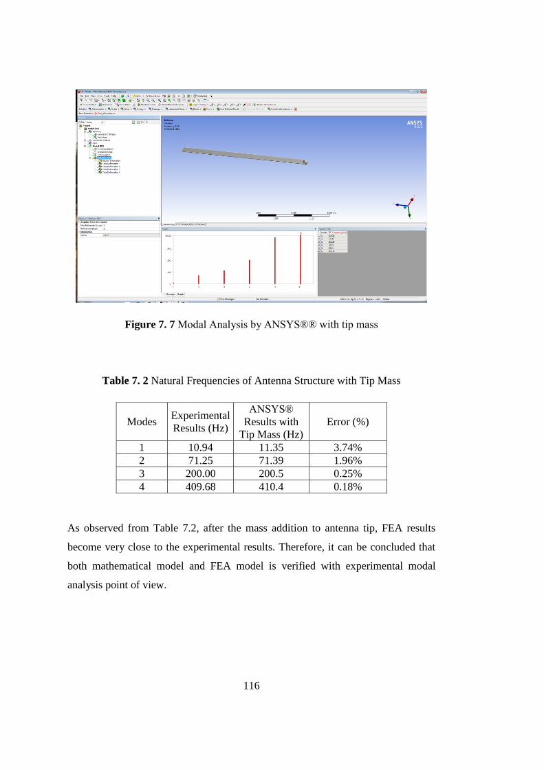
116
Figure 7. 7 Modal Analysis by ANSYS®® with tip mass
Table 7. 2 Natural Frequencies of Antenna Structure with Tip Mass
Modes Experimental
Results (Hz)
ANSYS®
Results with
Tip Mass (Hz)
Error (%)
1 10.94 11.35 3.74%
2 71.25 71.39 1.96%
3 200.00 200.5 0.25%
4 409.68 410.4 0.18%
As observed from Table 7.2, after the mass addition to antenna tip, FEA results
become very close to the experimental results. Therefore, it can be concluded that
both mathematical model and FEA model is verified with experimental modal
analysis point of view.

117
Modal damping ratios are found by means of half power point method [44]. The
formulation is presented as Equation (7.2).
Figure 7. 8 Response Curve Showing Half-Power Points and Bandwidth [44]
2 1 2 n (7.2)
Equation (7.2) holds if damping is light; therefore, light damping assumption is to
be checked after modal damping ratio calculations. From Table 7.3, it is concluded
that damping can be considered as light (below 10%). However, for transient
analysis verification, 5% modal damping should be updated (for mathematical and
FEA models) to the values presented in Table 7.3.

118
Table 7. 3 Modal Damping Ratios of Antenna Structure
Modes n 1 2 Modal damping
ratio ( )
1 10.938 10.776 11.239 0.0210
2 71.25 70.559 71.649 0.00765
3 200.00 197.876 206.189 0.0207
4 409.68 407.826 412.403 0.00559
Drop Experiment of Antenna Structure
Underwater shock explosion profile which antenna structure is exposed to, is
synthesized in Chapter 3 as half-sine profile. This introduces a convenience for the
experimental procedure. While double half sine pulses are very hard to generate in
small-to-medium scale laboratory conditions, half sine can easily be created by
drop test experiment. Shaker test can be proposed as another alternative for half-
sine input but it is limited up to 50-60 g’s from amplitude point of view. Thus, drop
test experiment is set to be performed for experimental transient analysis of antenna
structure. Drop test experiment is again performed on laboratory located in
ASELSAN. For drop test experiment, a drop table and built-in signal processing
system is used. Drop table used for experiment is LANSMONT® PDT 80 with
built-in controller and signal processing system produced by DataPhysics Corp.®.
Data sheets of both products are presented in Appendix B. Additionally,
IOTECH® data acquisition system mentioned in Section 7.2 with mini-
accelerometer PCB PIEZOTRONICS® 356A01 which is capable of up to 1000g
shock acceleration are used. Accelerometer is again placed at the antenna tip to
monitor and record shock response time history while another accelerometer is
placed onto the drop table to monitor shock input exposed to antenna base. FRFs
and time history data can be collected and monitored by means of IOTECH® and
eZ-Analyst® software. 200g-8ms shock input is adjusted by changing the drop

119
table properties. Release height affects the amplitude of shock while pad rebound
affects the effective shock duration. Therefore, as the preliminary work, proper pad
arrangement and release height is found by dummy drop experiments with and
without antenna structure. Dummy drop test without antenna structure is performed
in order to determine rebound coefficient of pads. After rebound coefficients are
determined approximately, release height is found easily. After one or two trial-
and-error, the exact height is determined. Shock duration is adjusted afterwards by
changing pad thickness.
For the first trial, formulation given in Equation (7.3) to (7.6) which are taken from
ANSI/ASA S2.62-2009 Standard [67] is used. Then, exact release height and pad
configuration is found with small adjustments.
2 1v v v (7.3)
2
VA
D
(7.4)
2
2
vh
g
(7.5)
2
1
2
res
r
v
eh
g
(7.6)
where; “ 1v ” is velocity before impact, “ 2v ” is velocity after impact, “h” is no
rebound drop height, “g” is gravitational acceleration, “D” is threshold pulse
duration, “A” is threshold pulse amplitude “ rese ” is coefficient of restitution and “
rh ” is drop height with rebound.
Exact release height is set to 153 mm with POM/C pad material and 8 unit 1/6” felt
above the pad. When everything is set, drop experiment is performed via controller

120
of the drop table and data is taken from both drop table for input signal profile and
from antenna tip in order to measure the antenna response.
Figure 7. 9 Drop Test Experiment
Input acceleration signal is measured from drop table jig base, and the output
response is measured from antenna tip as can be seen in Figure 7.9. Responses are
taken as the time history data for acceleration response at antenna tip.

121
Figure 7. 10 Shock Input Measurement Taken From Drop Table
Acceleration response measured from the antenna tip is compared to theoretical
model results in Figures 7.11 and 7.12.

122
Figure 7. 11 Mathematical Model and Experiment Comparison
0 0.05 0.1 0.15 0.2 0.25 0.3 0.35-300
-200
-100
0
100
200
300
400
X: 0.01384
Y: 321.3
Time (sec)
Accele
ration R
esponse [
G]
Comparison of Shock Responses at Antenna Tip
X: 0.01619
Y: 303.6
Experimental
Mathematical Model

123
Figure 7. 12 FEA Model and Experiment Comparison
Acceleration response measured from experiment is validated by checking the
frequency content of the signal. Frequency content of signal contains natural
frequencies of antenna structure, therefore, it is assured that acceleration data
contains meaningful data for antenna structure.
0 0.05 0.1 0.15 0.2 0.25 0.3 0.35-300
-200
-100
0
100
200
300
400
Time (sec)
Accele
ration R
esponse [
G]
Comparison of Shock Responses at Antenna Tip
X: 0.01619
Y: 303.6
X: 0.01391
Y: 315.8
Experimental
Finite Element Model

124
Figure 7. 13 Frequency Content of Measured Data
Results are tabulated in Table 7.4. The experimental result is taken as the reference
and modeling results are compared to experimental results.
Table 7. 4 Maximum Absolute Acceleration Results of All Analyses
Experimental Mathematical
Model ANSYS®
Absolute
Acceleration
(G)
303.6 321.3 315.8
Error - 5.83% 4.02%
Comments on Verification Results
In this chapter, verification of the theoretical models, namely, the mathematical
model and the FEA model is performed. Antenna model as Euler-Bernoulli beam
with Classical Approach is verified by means of hammer testing. In the light of test
results, natural frequencies are found to be very close to the experiment in 5-
percent error interval. After enhancement of antenna model with additional tip
mass (accelerometer mass), this error interval is reduced to almost 3-percent.

125
Therefore, mathematical and FEA models are verified with very fair natural
frequency results. Moreover, in order to update mathematical model, modal
damping ratios are calculated from FRF curve of experimental results by means of
Half Power Point Method. Tip-mass addition and damping ratio correction is
immediately performed for updated models. These models are used for transient
response comparison to experimental shock responses.
In the second part of this chapter, models are verified with drop test experiments
gathering transient response of the antenna. Comparing the acceleration responses
of mathematical model and experiments, response characteristics are found to be
very close. As frequency spectrum of experimental results contains natural
frequency peaks, experimental results are cross-checked. Maximum acceleration
response is the most important point to compare the results. As seen on Table 7.4,
both models give higher responses than experimental results. However, up to 5%
error for modeling shock phenomena is reported to be very satisfactory. Due to the
fact that model results are higher than experimental results, designs are to be
conservative and safe from failure as to be seen in Chapter 8. Noting that input half
sine profile measured for drop experiment is not an exact shape of desired half sine
input. However, the difference between the maximum acceleration response to
measured and theoretical responses is almost one percent. Thus, this small variation
is not taken into considerations for experimental shock analysis.
Upon considering Figure 7.11, general characteristics of responses are very similar.
However, shift of time axis for experimental results is observed after the effects of
harmonics are dominant. There are also some irregularities on the sinusoidal shape
of response curve. Possible reason for these differences is geometrical nonlinear
effects or nonlinear effects associated with boundary conditions which are not
considered in linear model. These effects are seen less on the FEA model, because
FEA model contains certain amount of nonlinear effect inherently. For the FEA
model, as seen in Figure 7.12, there is also a slight difference between damping
characteristics to experimental results. After updating the modal damping ratios,
only first two modal damping ratios can be defined to ANSYS® due to the use of

126
Rayleigh Damping Modeling. This yields some harmonical differences on last parts
of time history. As four modal damping ratio can be defined on mathematical
model, this differences are not observed that much.
After the experimental analysis is performed for antenna structure, it can be
concluded that mathematical model and FEA models are satisfactory enough for
use in design, qualification and isolation stages. In the lights of these verifications,
these models are readily employed for shock severity considerations at shock
survival stage of electromechanical design.

127
CHAPTER 8
8SHOCK SEVERITY FOR ANTENNA STRUCTURE
Shock input can have so severe effects that antenna performance may decrease in
unacceptable levels, electrical components attached on antenna may fail, and
antenna structure may face mechanical failure. Therefore, preliminary analysis is
performed by mathematical models and precautions are held in order not to face
with adverse effects of shock mentioned above. In this chapter, shock effects on the
antenna structure are examined, design limitations are drawn and precautions onto
the adverse effects of underwater shock are presented and verified with
experiments.
Shock Effects on Antenna Performance
One of the most important operational considerations in design of an antenna is the
direction of the radiation and angular location of the maximum radiation of antenna
pattern. If an antenna is bent through the axis where the pattern of it is symmetrical
with respect to that; this situation may lead to significant angular position shift on
the location of the maximum radiation on the antenna pattern. The shift mentioned
has directly affected the effective range of the antenna and some other parameters.
Moreover, this may lead to high error rates and false (artificial) results in case of
some applications such as direction finding (DF) and direction of arrival (DoA).
Dipole antenna structure examined in this study is with narrow bandwidth placed
through the z-axis. If it is deformed by 8 degrees, the decrease in gain may reach to
1.6 dB approximately at the plane of azimuth. This change in gain of the antenna
leads to decrease in effective range approximately 4700 km. The limitation of the
128
antenna is at most 1.6 dB gain decrease. In order to compensate the decrease in
effective range; higher power may be applied to the antenna. However, this is not
an effective solution because components of antenna may not withstand to this
level of power along with high power consumption. Therefore; the required
solution is to keep the bending degree of the antenna in an acceptable range where
the gain of the antenna varies on values that are appropriate according to proposed
utilization of the antenna. Thus; shock isolation of antenna structure should keep
the amount of bending of the antenna in the allowable range which comes from the
electrical design and pattern analysis of the antenna, that are, operational
constraints. The collinear antenna array of four dipole elements is given with the
effect of bending angle of the antenna pattern and gain. As a limitation comes from
antenna performance is maximum deflection of antenna structure should be in
region of -18.6 to +18.6 cm. Therefore, in electromechanical design stage of
antenna, from mathematical model or FEA model, maximum displacement is
observed and antenna performance decrease can be estimated. For the antenna
mentioned in this thesis, for synthesized shock value of 200g 8ms, relative
displacement curve is plotted as follows. The analysis is performed for damping
values found from the experimental analysis with the tip mass added to the
antenna.

129
Figure 8. 1 Relative Displacement of the Antenna Tip
From transient analysis, maximum relative displacement of antenna is found as
17.4 cm. The antenna performance decrease for corresponding bending value is
found as 1.57 dB on radiation patterns. Therefore, it is within the allowable limits
for proper functioning of the antenna. Furthermore, the mathematical model is
proved to be conservative comparing the experimental analysis. The antenna
performance is then expected to be higher than the predicted one and the antenna
performance can be regarded as “safe”.
In designer point of view, as a general design approach, shock effects on antenna
performance can be added to design process by applying the iterative design
procedure for the antenna structure. Shock analysis and electromagnetic analysis
can be performed together and optimum antenna design structure can be achieved
by changing antenna geometry, electromagnetic design or implementing isolation
concerns. Electromagnetic analysis results are given in Figure 8.2 and 8.3.
0 0.05 0.1 0.15 0.2 0.25 0.3 0.35 0.4-0.2
-0.15
-0.1
-0.05
0
0.05
0.1
0.15
X: 0.0255
Y: -0.174
Relative Displacement of Antenna Tip
Time (sec)
Rela
tice D
isp
lacem
en
t (m
)

130
Figure 8. 2 Electromagnetic Analysis of Dipole Antenna by HFSS®
Figure 8. 3 Radiation Pattern HFSS® Analysis of Antenna with Maximum
Allowable Deformed Position

131
Shock Severity Limits for Electrical Components on Antenna Structure
Antenna structure given in Figure 4.2 contains electrical components at vicinity of
antenna tip where the most vulnerable part to the shock effect is. Shock
environment produce dynamic stresses which may cause possible failure on
electrical components. The possible failure modes may include fatigue, ultimate
stress limit or yielding [55]. Hunt [56] presents the relationship between stress and
velocity on his seminal paper. Gaberson [57-59] enhanced the research on this
topic and presented the papers, presentations and some test results. Shock severity
limit is defined for military equipment with the study performed based on pseudo
velocity by Hunt, Gaberson, Morse, et al. These limits are used to determine
whether component qualification testing is necessary or not. In some cases further
action should be taken in order to maintain component survival.
Shock severity limit for electrical components are defined in military standards in a
very coarse form. In MIL-STD-810E standard, the empirical rule is proposed for
shock severity on components. Rule states that, shock should be considered as
severe only if defined threshold value is exceeded. Threshold value is defined in
Equation (8.1).
[0.8( / ) ( )]Threshold G Hz NaturalFrequency Hz (7.7)
MIL-STD-810E also states that, it is observed from military-quality equipment
tests, shock failures are not observed below a shock response spectrum velocity of
2.54 m/s [60]. However, both values are very conservative and far from reality;
because these effects are mostly considered for vibration case. For shock case,
shock severity should be considered thoroughly. The following theories are
presented for shock severity cases which are closer to the real-life applications.
From the experiments and studies followed on shock severity for components by
Gaberson and Morse [61-62], two different shock limit criteria are proposed. From
these studies, damage thresholds are proposed for different materials with 6 dB

132
tolerance interval. In Appendix C, for different materials velocity limits are
presented. As an example, velocity limits of shock severity for mild steel are
presented in Figure 8.1. From these tables, limitation for antenna structure as
AA6061-T6 beam is 10.51 m/sec with 6dB tolerance. Antenna response from the
mathematical model is given in Figure 8.4. Since maximum relative velocity value
is 16.1 m/s and it is bounded barely between 6-dB tolerance band; it is considered
as critical.
Figure 8. 4 Relative Velocity Response of the Antenna from Updated Models
0 0.05 0.1 0.15 0.2 0.25 0.3 0.35-20
-15
-10
-5
0
5
10
15
X: 0.0094
Y: -16.1
Relative Velocity at Antenna Tip
Time (Sec)
Rela
tive V
elo
cit
y (
m/s
)
Mathematical Model
FEA Model

133
Figure 8. 5 Morse Chart for Mild Steel Beams [62]
Another shock severity limit is Steinberg’s Relative displacement limit. Steinberg
[63] defined “Z” as a “single-amplitude displacement at the center of the electronic
board” which gives a fatigue life of about 20 million stress reversals in random
vibration environment. This definition is based on 3 circuit board relative
displacement.
Steinberg’s empirical formula is presented in Equation (8.2) in inches. Geometrical
parameters can be seen on Figure 8.2.
3 lim
0.0000426it
BZ
Chr L (7.8)

134
Figure 8. 6 Component Bending on the Antenna Structure [63]
In Equation (8.2), B is the length of the antenna edge parallel to the component, L
is the length of electronic component, h is the antenna thickness, r is the relative
position factor for the component mounted presented in Table 8.1 and C is the
constant for different types of electronic components presented in Appendix D.
Table 8. 1 Relative Position Factors for Component on Circuit Board
r Value Component Location
0.5 When component is at quarter point X and
quarter point Y
0.707 When component is at half point X and
quarter point Y
1 When component is at center of PCB
Finally, Steinberg’s relative displacement limit for shock input is calculated as six
times the 3-sigma-limit value. This shock limit is only valid for up to 200 cycles
created by strain hardening effect [63]. Thus, Steinberg’s empirical formula for
shock peak relative displacement limit in inches is presented in Equation (8.3).

135
3 lim6peak itZ Z (7.9)
Corresponding pseudo-velocity limit for shock severity is calculated as in Equation
(8.4).
2peak n peakPV f Z (7.10)
The limitations of Steinberg’s method are presented below.
Component's fatigue life may be below or over 20 million cycles.
3-sigma relative displacement may not be seen due to the non-stationary or
non-Gaussian distribution of random vibration.
Circuit board likely behaves as a MDOF system, therefore higher modes
should not be neglected. Thus, reversal cycle rate can be counted as greater
than that of the fundamental frequency alone.
Because of these limitations, it is not expected that results are exact but they show
the correct order-of-magnitude for antenna design and qualification stages.
Therefore, safe designs can be achieved with safety factor with this approach.
For antenna structure, mentioned in this thesis study, there are two resistors and
one capacitor placed on antenna span longitudinally. From Equations (8.2) and
(8.3) with Table 8.1 and Appendix D, antenna displacement should be below 22.29
cm. Comparing the maximum displacement of antenna tip given in Figure 8.1,
antenna structure considered to be safe.
Furthermore, for electrical resistor used for the antenna structure, it is advised that
component should be used below 250g mechanical shock loading (Appendix E).
Therefore, the antenna structure response should be below 250g. Since maximum
acceleration response is found as 321.3 G in Figure 7.11, this limitation is
considered as very critical.

136
Shock Stress Severity on Antenna Structure
For the antenna structure modeled in Figure 4.3 with the base acceleration shock
loading illustrated on Figure 4.4, shock stress and velocity relation is presented in
this section with different methods [64].
8.3.1 Shock Stress from Single Mode Modal Transient Analysis
In this method modal transient analysis is performed for fundamental natural
frequency of antenna structure. Transient relative velocity response is considered
among modal transient responses. The maximum bending stress formulation is
given in Equation (8.5).
max ,maxˆ
n
Emc v
IL (7.11)
In Equation (8.5), c is distance to neutral axis, E is elastic modulus, m is antenna
mass, “I” is area moment of inertia, “L” is antenna length and “ ,maxnv ” is modal
maximum relative velocity response. Maximum bending stress at fixed boundary
is, thus, calculated from the maximum relative velocity at the free end by means of
transient analysis using only fundamental frequency of the antenna. Results can be
compared to bending stress calculated from the second derivative of mode shape of
the antenna structure.

137
8.3.2 Shock Stress from Single Mode Direct SRS
In this method, acceleration SRS curve is taken into consideration for fundamental
velocity. From acceleration output at fundamental frequency, pseudo-velocity can
be calculated as presented in Equation (8.6) where V is a pseudo-velocity.
n
zV
(7.12)
As a next step, the approximate relative velocity can be calculated for single mode
model as presented in 8.7.
max 1 1,maxˆz q V (7.13)
In Equation (8.7), 1 is participation factor for the first mode, 1,maxq is maximum
mass-normalized eigenfunction for the first mode and V is pseudo-velocity found
in Equation (8.6). Maximum relative velocity value may be used for maximum
bending stress calculation presented in Equation 8.5.
8.3.3 Shock Stress from Four Mode Transient Analysis
In this method just the same formulation is followed as the method presented in
Section 8.3.1. As a difference, in four fundamental modes are used for transient
analysis. It is proved in Section 5.1 that four-mode configuration is enough for 90
percent modal mass participation. The most accurate result is expected to be
obtained by this method among others.

138
8.3.4 Allowable Stress for Naval Applications
Allowable stress for naval applications is defined as NRL sum of the stresses in the
form of total membrane stress, total membrane plus bending stress, total buckling
stress and total bearing stress. Antenna structure is subjected to bending stresses at
fixed end and stress concentration is observed around bended region. Therefore,
total membrane plus bending stress is applied on antenna structure. The factors
defined are due to experimental results in the safe margin. Since the shock energy
is applied on structure within very small interval, the actual effect is less than
expected. Components which are attached to naval platform is categorized as Grade
A and Grade B type components according to their importance. “Grade A items are
systems or equipment which are essential to the safety and continued mission
capability of the ship. Grade B items, which are not essential to safety or the
combat mission, are those items that could became a hazard to personnel or to
Grade A items. [6]” Antenna structure is, hence, classified as Grade A component.
For Grade A and Grade B components, allowable stress limits are tabulated in
Table 8.2.

139
Table 8. 2 Grade A Allowable Stress Criteria and Applicable Design Levels [6]
Using Equation (8.5) with 4-mode updated (tip mass and modal damping) transient
response analysis of antenna structure performed in Chapter 7, the maximum stress
is found as 386.4 MPa. From Table 8.2, for Grade A components, allowable stress
is two-times of yield stress of structure. Yield stress for AA6061-T6 is 276 MPa.
Therefore, the maximum allowable stress is 552 MPa for the antenna structure,
which is above the maximum stress and antenna structure can be considered as
“safe”. Stress analysis is further performed by ANSYS® Transient analysis and the
maximum stress is observed at antenna head as around 413 MPa. However, this
value is kind of artificial due to the fact that stress waves are moving from free end
to the cantilever base and cancelling each other while coming back to the antenna
tip due to the direction change.
140
Further study is performed about stress consideration while shock testing. In
experimental analysis, shock input level of antenna structure is increased gradually
and reached up to 2658 g – 6ms half-sine input. After tests are performed, there is
any failure or deformation observed on antenna structure. Therefore, it is stated
that, for shock phenomenon, since effective shock duration is limited real effects of
shock as stress on antenna structure is less than expected. Therefore, NRL
limitation of allowable stress on structures subjected to underwater explosions is
very conservative and structures below these limits can be considered as “safe”
enough.
Antenna Limitations Caused by Shock Severity
Antenna limitations have been explained in previous sections. For these limitations,
antenna structure should be re-designed or isolation precautions should be taken.
Since electromagnetic design limits any change of antenna dimensions and of
material change. For example, in order to increase maximum velocity limit, the
material can be changed to AA6061-T6 to Titanium Alloy. However, this brings
additional tangent loss to the antenna performance and additional mass to the total
system. Therefore, it is not possible to apply geometrical or material change in
antenna structure. Instead of design change, shock isolation is performed to achieve
the safe design for certain limitations. In Table 8.3, shock severity limitations are
presented.

141
Table 8. 3 Shock Severity Limitations
Criteria Response
Limitation Limit
Maximum
Value from
Mathematical
Model
Severity
Antenna
Performance
Relative
Displacement
(cm)
18.6 17.4 Safe
Electrical
Component
Analysis
(Morse)
Relative
Velocity
(m/s) 10.51 16.1 Critical
Electrical
Component
Analysis
(Steinberg)
Relative
Displacement
(cm)
22.29 17.4 Safe
Resistor
Mechanical
Shock Limit
Absolute
Acceleration
(G)
250 321.1 Very
Critical
Maximum
Allowable
Stress
Stress (MPa) 552 386.4 Safe
Shock Isolation of Antenna Structure
In recent years, shock problems of antenna structures mounted on naval platforms
have arisen, and they are expected to continue. In order to sustain the performance
of antenna structure and to take precautions to the possible concerns mentioned on
Sections 8.1 to 8.3, shock isolation should be performed. Because of these reasons,
the study on selection of shock isolation materials and shock isolation theory is
presented.

142
8.5.1 General View on Shock Isolation
Sensitive components like antenna structures are required to be treated with shock
isolation where precautions cannot be taken in modal design or structural
modification stages. Therefore, shock amplitude is tried to be reduced by means of
force or energy transfer to the isolator material. Especially, materials with low
stiffness have decreasing effects on shock forces acting on the structure to be
isolated. Isolators cannot damp shock effects if frequency is very low and may
amplify the shock effects if frequency of interest is close to the natural frequency.
System is successful in isolation standpoint, if the natural frequency of isolator
together with the antenna structure is considerably low. However, isolator material
should not be so soft due to the endurance and stabilization problems. Therefore,
the optimum isolator material is to be selected. Attachment of isolator to the
antenna structure should be designed so that loading is distributed to each while the
same amount of deformation is observed.
For systems subjected to shock excitation used for naval applications, antenna
structure and other components survived by means of shock isolators. Shock
isolators absorb the energy of shock motion by means of squeezing in a short time
interval, then release this energy by means of elongation in relatively long time
interval. In other words, isolators convert high amplitude-short duration shock
signal to relatively low amplitude-long duration response (Figure 8.7).

143
Figure 8. 7 Shock Damping by means of Isolators on, a) Acceleration-time plot,
b) Force-displacement plot [63]
Important remarks on proper use of shock isolator are following: Isolator selected
should meet the dynamic displacement required. Otherwise, isolator may amplify
the shock effects which may be observed with qualification tests or on operations.
Since large displacements occur in shock isolation, stiffness of isolator should not
be linear. Success of isolation is monitored by the displacement of isolator
required. For many operations, linear isolators cannot supply large displacements,
therefore nonlinear isolators should be opted instead of linear ones. For example,
wire rope type isolators are very suitable for shock applications. Because, they are
capable of high energy storage and their form can change easily. Therefore, they
may show linear and non-linear characteristics together. If metal isolators cannot be
used for applications like antenna isolation, gel type isolators can be used. These
types of isolators can also show both linear and non-linear characteristics like wire
rope. However, shock isolation level of gel type isolators are not that high as wire
rope.

144
8.5.2 Shock Isolator Selection
It is essential to select appropriate shock isolator in order not to face with adverse
effects of shock on warfare structures such as antennas. In this part, shock isolator
selection steps are presented. For the calculation step, Equations (8.8) and (8.9)
along with Figure (8.8) are taken from isolator selection catalogue [65].
Generally, the first step of isolator selection starts with taking integrals of shock
input profile in order to find velocity values. Velocity value shockV is the initial
velocity of the system reached by means of the response to the shock input. shockV
values along with different forms of shock inputs are presented in Figure 8.8. After
that step, considering the shock output outg as a magnitude of desired acceleration
response, natural frequency of the system is calculated by Equation (8.8), noting
that g is “gravitational acceleration”.
,2
outn system
shock
g gf
V (7.14)

145
Figure 8. 8 Shock Velocity Formulation for Different Types of Shock [65]
Then, the displacement value that isolator should reach is found with Equation 8.9.
,2
shock
n system
VD
f (7.15)
Finally, isolator should be selected considering the following rules.
Natural frequency of isolator should be lower than the natural frequency of
the system calculated in Equation (8.9).
Minimum displacement value of shock isolator should be higher than the
displacement value calculated in Equation (8.9).
Isolator material should not be of metal due to the electromagnetic
reflection with antenna structure.

146
For antenna structure considered in study, limitation is set to 240 G output
acceleration because the shock severity limitation is found as 250 G in Section 8.4.
For this acceleration value, relative velocity criteria is checked and verified as to be
safe. Thus, it is guaranteed that all limitations are covered with this value.
Moreover, mathematical model results are higher than experimental results. This
also brings more safety for conservative isolator selection.
Therefore, for limitation of 240 G, shockV is found as 10.01 m/s, ,n systemf is found as
37.5 Hz and D is found as 0.042 m.
Next step of isolator selection is to select possible isolator type. For isolator type
selection, dimension and material limitation are very important. Since antenna
structure have width of 0.02 m at base interface, miniature isolator that meet the
requirements should be selected.
In electromagnetic point-of-view platform analysis with isolator material is
performed. In this analysis, the higher loss tangent value of the isolator material,
the lower unexpected reflection losses will be. Therefore, wire materials cannot be
selected as isolator materials. For the detailed research of insulation materials used
for shock isolators, material loss tangents are measured by experimental setup for
Original GEL, Beta-GEL, Theta-GEL, Urethane, Rubber, Natural Rubber and
APDM rubber samples. GEL type isolators are selected due to the minimum effect
on antenna performance. From data sheets of Taica® GEL isolator, MN Type
Theta-GEL isolator with approximately 17 Hz natural frequency and up to 10 cm
displacement capability is selected. Data Sheet of the product is given in Appendix
F.

147
Isolator Verification by Drop Experiment
Drop experiment is repeated in order to observe isolator performance and check the
achievement of shock severity requirements.
Figure 8. 9 Drop Experiment of Antenna with Isolator
Measured acceleration response at antenna tip is presented in Figure 8.10 with
acceleration response measured without isolator.

148
Figure 8. 10 Acceleration Response for the Antenna with Isolator
As observed from the response plot with isolator, 28.3% reduction of maximum
acceleration is measured and desired output acceleration limit (240G) is achieved
with some safety margin. Therefore, the isolator verification holds. In order to
observe relative velocity response, acceleration response is integrated in frequency
domain data obtained by Fast Fourier Transform, then Inverse Fast Fourier
Transform yields the time domain relative velocity data with certain amount of
error. MATLAB® script written for this calculation is presented in Appendix G. As
seen on Figure 8.11, maximum relative velocity value of the antenna structure is
decreased to under allowable limits. For that maximum relative velocity,
corresponding stress is calculated as 212.6 MPa which is seventy seven percent of
yield strength of aluminum. Therefore, stress value is reduced to below yield
strength with considerable safety margin.
0 0.05 0.1 0.15 0.2 0.25 0.3-300
-200
-100
0
100
200
300
X: 0.01619
Y: 295.6
Time (sec)
Accele
ration R
esponse [
G]
Comparison of Shock Responses at Antenna Tip
X: 0.009682
Y: -212
Without Isolator
With Islator

149
Figure 8. 11 Relative Velocity Response of the Antenna with Isolator
Discussion
Antenna performance is determined and evaluated from both electromagnetic
design and mechanical properties standpoints. Therefore, mechanical shock may
have severe effects on both antenna performance and mechanical survival. In order
to eliminate these severe effects, some precautions should be taken at mechanical
design stage like geometrical or material changes in design and shock isolation. In
this chapter, severe effects of shock on antenna structure are presented and design
limitations are determined. As there is no chance on design changes of antenna
structure, shock isolation is introduced and isolation procedure is explained in
detail. Then, the isolator selection of antenna is performed step-by-step considering
0 0.05 0.1 0.15 0.2 0.25 0.3-8
-6
-4
-2
0
2
4
6
8
10
X: 0.08146
Y: 9.702
Relative Velocity Response of Antenna with Isolator
Time [s]
Velo
city[m
/s]

150
the design limitations. Throughout these stages from shock severity limitations to
isolator selection, mathematical models are used. After design improvements are
performed with isolator addition on system, experimental verification is performed.
Experimental results of the system with isolator are compared to those of the
system without isolator. Almost 30% reduction in maximum acceleration is
obtained with acceptable maximum relative velocity value. As relative
displacement values of non-isolated system is safe enough, no further development
is performed. Antenna with isolator response behavior is different than antenna
without isolator because of the nonlinear effects of isolator material. These
different behaviors are observed as natural frequency shift, double peaks at
maximum points, fast damping and more harmonics on secondary responses. As
antenna structure is approximated by a cantilever beam, strain energy is only
obtained from antenna fixed end. Limited location selection for the antenna
structure makes isolation performance lower than other applications. GEL type
isolators propose the maximum possible performance among others.
This chapter is presented as design guide for shock severity. Mathematical model
built throughout this thesis is used to foresee severe effects on shock without
performing any qualification tests. Interactive design is also possible for both
mechanical and electromagnetic point-of-view, as iterative design can be
accomplished by means of proposed design methodology.

151
CHAPTER 9
9SUMMARY AND CONCLUSIONS
Summary
This study aims to perform complete shock analysis of dipole antenna structure
used for ESM/COMINT applications subjected to underwater explosions. The
purpose is to protect antenna structure from shock effects and maintain its function
in warfare. In mechanical point-of-view, shock considerations for design is very
important and not fully solved problems. In order to eliminate adverse effects of
shock loading on antenna performance, shock response of an antenna structure is
investigated in detailed way. Experimentally verified linear model of antenna
structure is used to perform transient response analysis to foresee the shock
characteristics. These inputs can be used a starting points to initiate
electromechanical design procedure of antenna structures. They can be used in
replacement of qualification tests which are hard to perform or they can be used as
design updates for the antennas which fail or tend to fail. The mathematical models
are capable to perform these analysis for various beam geometries with different
boundary conditions. Model is also capable to perform transient response analysis
for different shock inputs even if it is wavelet input. Shock severity considerations
are another important issue for shock analysis. As an electromechanical device,
antenna structure consists of some electronic parts attached to its mechanical base.
Therefore, shock severity considerations consist design limitations for electronic
devices as do for mechanical structure. To eliminate these effects and to maintain
antenna functioning, shock isolation procedure is introduced with shock isolation
theory and verified application on the antenna structure.

152
In the scope of this study, dipole antenna which is attached to submarine periscope
with fixed-free boundary conditions is considered. In order to generate shock input
classified with standards, shock profile synthesis is performed thus; easily
producible shock input is obtained. Antenna structure is modeled as a cantilever
beam with Classical Theory and its modal properties are determined. Then,
transient shock analysis is performed with MDOF Recursive Filtering Relationship
Method which gives the closest results to the exact solution among SDOF methods
and other approximate methods. FEA analysis is also performed for antenna
structure with full model transient response analysis. Because FEA model and
mathematical model yields closer results and they are both verified by experimental
studies. They can be interchangeably used according to the ease of use.
Experimental verification of these models is performed by hammer tests for modal
verification and drop experiment for transient response verification. Finally, shock
severity limitations are explained both for electronic and mechanical elements of
antenna. Shock isolation is performed in order to overcome these limitations.
Complete shock analysis can be enhanced for different antennas with different
application areas. Therefore, apart from underwater shock inputs; gunfire, ballistic,
field vehicle shock inputs can be synthesized or used as they are. Mathematical
model is capable to perform such different analyses with simple selections in
MATLAB® script.
Shock isolation and design guide for shock severity is also verified in Chapter 8 for
antenna structure that is to be qualified or designed. Therefore, this design guide is
a very useful tool to perform shock analysis for designers and it is very practical to
use for whom are not familiar to shock and vibration topics.
153
Conclusions
By means of the proposed methodology throughout the study, multi-degree-of-
freedom transient response analysis of the antenna structure is accurately
performed using four modes (90% of the effective modal mass) of the structure.
Transient response analysis of the similar (beam type) antenna structures with
different dimensions and different field of applications can be readily applied.
Performing the shock profile synthesis, it is observed that different type of shock
inputs can be synthesized for reproducibility. Synthesized profiles are more
conservative than original ones due to the fact that shock response spectrum
coverage is higher than original pulses for low frequencies as seen in Figure 3.12.
Euler-Bernoulli Beam assumption is made for antenna structure as a slender beam.
Assumptions of Euler-Bernoulli beam theory do not under estimate the responses
of antenna structures. Modal analysis verifications with very small errors shows
that for antenna structures with similar geometry, these assumptions can be done
for brevity. For further investigation such as shear effects, Timoshenko Beam
Theory can be applied. For such kind of applications, mathematical model can be
updated or FE model proposed in this study can be used directly.
For transient analysis of the antenna structure, RFR method is used for solution
algorithm. This method is very easy to apply on shock response analysis
formulation and it is very fast. Elapsed time for response obtained from this
method is almost a second for both modal and transient analysis. For ANSYS®
solution it is almost ten seconds for complete solution. Therefore, method
developed for transient solution can be considered as very fast and accurate.
Different boundary condition selection, material selection, included number of
mode selection, modal damping selection, desired response location, different
shock input type selection are possible with this model.

154
SDOF Models and approximate models are easier to build and apply than MDOF
analysis. However, if these methods are used, user should be aware of the error
possibility from 10% to 100%. Therefore, this may mislead the designer for shock
severity considerations.
It is important to acquire reliable responses from experimental analysis if transient
analysis is concerned. High coherence values at natural frequencies, spectrum
content of transient response and modal updating according to experimental
feedbacks assures the reliability of mathematical model and FE solution. Results
obtained from analyses and experiments are used for crosscheck in corresponding
chapters in this manner.
Theoretical maximum allowable stress values for structures under transient loading
are so safe enough not to face with failure of antenna material. In experimental
analysis stages, maximum allowable shock loading limits are exceeded and no
failure and deformation is observed. Stress values are calculated higher than yield
stress of the material due to the forcing duration is very small and forcing
behaviors are different than static loading cases.
It is observed that shock isolation material is very effective on antenna
performance. Using inappropriate isolator type like wire rope or natural rubber may
result in severe decrease on antenna performance. Therefore, material type should
be added to isolator criteria steps.
Future Work
This study can be improved by implementing further capabilities:
Geometric nonlinearities can be added to model.
Boundary condition nonlinearities can be added to model.
Solution methodologies can be combined in order to obtain faster and more
accurate responses. These methodologies can be implemented to ANSYS®

155
to perform interactive response analysis. Therefore, simplicity of analysis
and fast solver results with very high accuracy can be obtained.
Experimental stress analysis can be performed for the antenna structure
under shock loading. Stress distribution of antenna structure can be
analyzed for three loading conditions (vertical, transverse and longitudinal)
and failure conditions of antenna should be defined clearly. Antenna
structure may also be investigated for vertical loading in case of stress
variations caused by buckling motion. As the vertical shock loading
specifications for naval applications are very high, buckling motion is to be
examined for continuous and failure-free operations for antenna structure.
Isolator material can be selected different than GEL type with lower loss
tangent value.
Isolation can be added to mathematical model and they can be investigated
together.
Experimental analysis can be performed with laser vibrometer to measure
displacement response.
Optimization may be studied in order to obtain maximum performance
from isolation process.

156

157
REFERENCES
[1] Tembarai Krishnamachari, R. "Dawn of the E-bomb: High-power microwave
technology and military implications for India", South Asia Analysis Group, Paper
1089, May 2004.
[2] "Joint Publication 3-13.1 Electronic Warfare". Chairman of the Joint Chiefs of
Staff (CJCS) - Armed Forces of the United States of America. 25 January 2007. pp.
i, v – x. Retrieved 2011-05-01.
[3] IEEE Std. 145™-2013, IEEE Antennas and Propagation Society, "IEEE
Standard for Definitions of Terms for Antennas", New York, USA, December 2013.
[4] Walter, P.L., “Selecting Accelerometers for Mechanical Shock
Measurements”, PCB Piezotronics, Depew, New York, TN-24, December 2007.
[5] MIL-STD-810G, “Environmental Engineering Considerations and Laboratory
Tests”, Department of Defense Test Method Standard, USA, 2008.
[6] Scavuzzo R.J., Pusey, H., “Naval Shock Analysis and Design”, HI-Test
Laboratories Inc., 6th Printing, Virginia, 2013.
[7] Mercimek, Ümit. “Shock Failure Analysis Of Military Equipments By Using
Strain Energy Density”, MSc Thesis, Mechanical Engineering, Middle East
Technical University, December 2010.
[8] Harris, C.M., Piersol, A.G., Hill, M., Shock and Vibration Handbook, Fifth
Edition, 2002.

158
[9] Mair, Hans U., “Simulated Ship Shock Tests/Trials?”, Institute for Defense
Analyses, Virginia, USA.
[10] Galileo, Galilei, “Discorsi e dimonstrazioni matematiche intorno a due nuove
scienze attinenti la meccanica e i movimenti locali”, publication Cierre, Simeoni
Arti Grafiche, Verona, 2011.
[11] Biot,M.A., “Theory of Elastic Systems Vibrating Under Transient Impulse”,
Proc. Natl. Acad. Sci. U.S., Vol.19, pp.262, 1993.
[12] Biot, M.A., “A Mechanical Analyze for the Prediction of Earthquake
Stresses”, Bull. Seismological Soc. Am., Vol.31, No.2, pp.151, 1941.
[13] Biot, M.A., “Analytical and Experimental Methods in Engineering
Seismology”, Trans. ASCE, No.108, pp.365, 1943.
[14] Biot, M.A., “Transient Oscillations in Elastic Systems”, Ph.D. Thesis No.259,
Aeronautics Department, California Institute of Technology, 1932.
[15] Mindlin, R.A., “Conversation with the author”, 1942.
[16] Housner, G.W., “Behavior of Structures during Earthquakes,” J. of Eng.
Mech. Div., ASCE, Vol. 85, No. EM4, pp. 109-129, 1959.
[17] Newmark, N.M., Rosenblueth, “Fundamentals of Earthquake Engineering”,
Prentice-Hall, 1971.
[18] Newmark, N.M., “A Method of Computation for Structural Dynamics”,
ASCE Journal of the Engineering Mechanics Division, Vol. 85 No. EM3, 1959.

159
[19] Alexander, J.E., “Shock Response Spectrum – A Primer”, BAE Systems, US
Combat Systems Minneapolis, Minneapolis, Minnesota, Sound and Vibration, pp.
6-14, June 2009.
[20] Tuma, J., Koci, P., “Calculation of Shock Response Spectrum”, Colloquium
Dynamics of Machines 2009, Prague, February 2009.
[21] Smallwood, D. O., “An Improved Recursive Formula for Calculating Shock
Response Spectra”, 51st Shock and Vibration Bulletin, Sandia National
Laboratories, Albuquerque, New Mexico, 1980.
[22] Kelly, R.D., Richman, G., “Principles and Techniques of Shock Data
Analysis”, The Shock and Vibration Information Center, Washington, D.C., 1969.
[23] Irvine, T., “An Introduction to the Shock Response Spectrum”, Vibration
Data, July 2010.
[24] Dorf, R., “Modern Control Systems”, Addison-Wiley, Reading,
Massachusetts, 1980.
[25] Irvine, T., “Shock Response of Multi-Degree-of-Freedom Systems”, Revision
F, Vibration Data, July 2010.
[26] Parlak, M., “Bir Hava Savunma Sisteminin Deneysel Sok Analizi”, 11. Ulusal
Makina Teorisi Sempozyumu, Gazi Üniversitesi, Mühendislik-Mimarlık Fakültesi,
Ankara, Eylül 2003.
[27] Burgess, A. , “Transient Response of Mechanical Structures using Modal
Analysis Techniques” , Department of Mechanical Engineering, Imperial College,
London SW7, January 1988.

160
[28] Bhat, P., Chandrasekhar, J., “Shock Response Spectrum Analysis Approach
for Optimal Design of Electronic Devices”, Axiom Consulting Pvt. Ltd.,
Bangalore, India.
[29] Wang, G., Xiong Y., Tang, W., “A Novel Heavy-weight Shock Test Machine
for Simulating Underwater Explosive Shock Environment: Mathematical Modeling
and Mechanism Analysis”, School of Logistics Engineering, Wuhan University of
Technology, China, July 2013.
[30] Campos, D.J.G., “A Study of Shock Analysis Using The Finite Element
Method Verified with Euler-Bernoulli Beam Theory; Mechanical Effects Due to
Pulse Width Variation of Shock Inputs; and Evaluation of Shock Response of a
Mixed Flow Fan”, Faculty of California Polytechnic State University, July 2014.
[31] Haukaas, T., “Euler-Bernoulli Beams." University of British Columbia,
November 2012.
[32] Yang, Bingen. “Stress, Strain, and Structural Dynamics: An Interactive
Handbook of Formulas, Solutions, and MATLAB® Toolboxes”, Elsevier Inc., San
Diego, 2005.
[33] Remala, S.N.R., “Nonlinear Transient Finite Element Simulations of Beam
Parametric Response Including Quadratic Damping”, University of Kentucky,
2005.
[34] DeBruin, J., “Shock Isolation for Mobile Pointed Satcom Systems”, General
Dynamics SATCOM Technologies, Texas.
[35] Parlak, M., “Vibration Isolation of a Platform with a Shock Disturbance”,
Middle East Technical University, Ankara, Turkey, December 2002.

161
[36] Klembczyk, A.R., “Introduction to Shock and Vibration Isolation and
Damping Systems”, Taylor Devices, Inc., New York, 2010.
[37] Tustin,W., Hieber,G.M., “Understanding and Measuring the Shock Response
Spectrum”, The Applications Engineering Staff Spectral Dynamics Corporation of
San Diego, USA.
[38] “Shock Response Spectrum”, SRSView. Available:
http://www.signalysis.com/ , Retrieved on March 10, 2014.
[39] Building Specification for Ships of the Federal Armed Forces, 043, Shock
Resistance Experimental and Mathematical Proof, March 1985.
[40] Majkut, L. “Free and Forced Vibrations of Timoshenko Beams Described by
Single Difference Equations.” Journal of Theoretical and Applied Mechanics 47.1
(2009): 193-210.
[41] Tonguei B. H. “Principles of Vibration”, New York. Oxford University Pressi
Inc. 1996.
[42] Whitney, S. “Vibrations of Cantilever Beams: Deflection, Frequency and
Research Uses”, University of Nebraska-Lincoln. April 1999.
[43] Sadd, M.H. “Wave Motion and Vibration in Continuous Media”, Kingston:
University of Rhode Island, 2009.
[44] Rao, S.S. “Mechanical Vibrations”, Fifth Edition in SI Units, Pearson Inc.,
Singapore, 2011.
[45] Irvine, T., “Modal Transient Vibration Response of a Cantilever Beam
Subjected to Base Excitation”, Vibration Data, January 2013.

162
[46] Thomson, W. “Theory of Vibration with Applications”, Second Edition,
Prentice Hall, New Jersey, 1981.
[47] Irvine, T., “Modal Transient Analysis of a System Subjected to an Applied
Force via a Ramp Invariant Digital Recursive Filtering Relationship”, Revision K,
Vibration Data, 2012.
[48] Brandt A., Ahlin, K. “A Digital Filter Method for Forced Response
Computation”, Society for Experimental Mechanics (SEM) Proceedings, IMAC-
XXI.
[49] Irvine, T., “The Generalized Coordinate Method for Discrete Systems”,
Revision F, Vibration Data, 2012.
[50] Dukkipati, R.V., “Vehicle Dynamics” CRC Press, Narosa Publishing House,
New York, 2000.
[51] Bathe, K., “Finite Element Procedures in Engineering Analysis”, Prantice-
Hall, Englewood Cliffs, New Jersey, 1982.
[52] “Implicit Versus Explicit Methods”, Flow science Inc,
http://www.flow3d.com/ .Retrieved on June 24, 2015.
[53] Irvine, T., “Shock Response for Multi-Degree-Of-Freedom Systems”,
Vibration Data, May 2010.
[54] Wilson E., “Dynamic Analysis by Numerical Integration”, Static and Dynamic
Analysis, Technical Paper, 1998. Retrieved on July 18, 2015.
[55] Irvine, T., “Shock and Vibration Stress As a Function of Velocity”, Vibration
Data, April 2013.

163
[56] Hunt, F.V., “Stress and Strain Limits on the Attainable Velocity in
Mechanical Systems”, JASA, 32(9) 1123-1128, 1960.
[57] Gaberson and Chalmers, “Modal Velocity as a Criterion of Shock Severity”,
Shock and Vibration Bulletin, Naval Research Lab., December 1969.
[58] Gaberson, H., “Using the Velocity Spectrum for Damage Potential”,
SAVIAC, 74th Symposium, San Diego, CA, 2003.
[59] Gaberson, H., “An Overview of the Use of the Pseudo Velocity Shock
Spectrum”, Space Craft and Lunch Vehicle, Dynamic Environments Workshop,
The Aerospace Corporation, El Segundo, CA, 2007.
[60] MIL-STD-810E, “Environmental Engineering Considerations and Laboratory
Tests”, Department of Defense Test Method Standard, USA, 1989.
[61] Gaberson, H., “Shock Severity Estimation”, Sound and Vibration, January,
2012.
[62] Morse, R., “Presentation of Spacecraft & Launch Vehicle Dynamics
Environments Workshop Program”, Aerospace Corp, El Sagundo, CA, June, 2000.
[63] Steinberg, D.S., “Vibration Analysis for Electronic Equipment”, Second
Edition, Wiley-Interscience, New York, 1988.
[64] Irvine, T., “Shock and Vibration Stress-Velocity Examples for Beam
Bending”, Vibration Data, April 2013.
[65] Barry Controls Shock and Vibration Isolators Guide, England, 2002.

164
[66] Irvine, T., “Shock Severity Limits for Electrical Components”, Revision D,
Vibration Data, June 2014.
[67] ANSI/ASA S2.62-2009, “Shock Test Requirements for Equipment in a
Rugged Shock Environment”, http://asastore.aip.org. Retrieved on April 16, 2015.
[68] Sloan, J. L, “Design and Packaging Electronic Equipment”, Van
Nost.Reinhold, February 1985.
[69] Roark, R. J. ''Formulas for Stress and Strain,'' 4th ed., McGraw-Hill, 1965.
[70] "MIL-S-901D (Navy), Military Specification: Shock Tests. H.I. (High-
Impact) Shipboard Machinery, Equipment, and Systems, Requirements For" .
United States, Department of Defense. March 17, 1989.
[71] Iotech Inc. “High Speed Portable Data Acquisition Systems User’s Manual”,
Rev. 5.0.
[72] PCB Piezotronics, “Technical Data Sheets”, www.pcb.com/accelerometers.
Retrieved on August 18, 2015.
[73] Lansmont Corp., “PDT 80 Product Specifications”,
www.lansmont.com/products/shock. Retrieved on August 17, 2015.
[74] American Technical Ceramics, “ATC High Power Flange Mount Resistors
Technical Data Sheet”, www.atceramics.com/atc_products. Retrieved on August
18, 2015.
[75] Taica Co., “Taica Alpha Gel MN Series Isolator Technical Details”,
www.taica.co.jp/gel-english/products/insulator.htm. Retrieved on May 28, 2015.

165
APPENDIX A
10CALCULATIONS OF SRS VALUES FROM BV043
STANDARD
From Equations (3.10) to (3.14) and the tabulated values given in Table 3.1,
acceleration-time signal for the equipment installed on submarine of class >2000t
can be calculated.
For Z-direction,
01
2
3
VV (A.1)
1 6.667m
Vs
2 00.5a A (A.2)
3
2 22 10
ma
s
22g
aa
g (A.3)
2 204.943ga
11
22
Vt
a
(A.4)
3
1 5.236 10t s

166
02 1
1
2dt t
V
(A.5)
3
2 6.764 10t s
14
22
Va
t
(A.6)
3
4 21.548 10
ma
s
44g
aa
g (A.7)
4 157.871ga
For Y-direction,
3
2 21.75 10
ma
s
2 178.45ga
3
1 5.086 10t s
3
2 9.031 10t s
4 2985.597
ma
s
4 100.503ga
For X-direction,

167
1 2.833m
Vs
2 2875
ma
s
2 89.825ga
3
1 5.086 10t s
3
2 9.031 10t s
4 2492.798
ma
s
4 50.251ga

168

169
APPENDIX B
11EQUIPMENT USED THROUGHOUT TESTS
Figure B. 1 General Specifications of IOTECH® WaveBook Data Acquisition
System [71]

170
Figure B. 2 General Specifications of PIEZOTRONICS® 356A01
Accelerometer [72]

171
Figure B. 3 General Specifications of PIEZOTRONICS® 086E80 Impact
Hammer [72]

172
Figure B. 4 General Specifications of LANSMONT® PDT 80 Drop Table [73]

173
APPENDIX C
12VELOCITY LIMITS OF MATERIALS
Table C. 1 Severe Velocities, Fundamental Limits to Modal Velocities in
Structures [59]
Table C. 2 Values from Roark, 1965, p 416 [69]

174
Table C. 3 Severe Velocity Values from Sloan, 1985 [68]

175
APPENDIX D
13“C” CONSTANTS FOR DIFFERENT TYPES OF
ELECTRICAL COMPONENTS
Table D. 1 Constant for Different Types of Electronic Components [66]

176
Table D. 1 Constant for Different Types of Electronic Components (continued)
[66]

177
Table D. 1 Constant for Different Types of Electronic Components (continued)
[66]

178

179
APPENDIX E
14ATC® HIGH POWER FLANGE MOUNT RESISTOR
Figure E. 1 General Specifications of ATC® High Power Flange Mount
Resistor [74]

180

181
APPENDIX F
15TAICA ALPHA-GEL® MN SERIES ISOLATOR
Figure F. 1 General Specifications of Taica ALPHA-GEL® MN Series Isolator
[75]

182

183
APPENDIX G
16MATLAB® SCRIPT FOR FREQUENCY DOMAIN
DIFFERENTIATION
17
clear all;close all;clc data=fopen('deney_MATLAB®_iso.txt'); accdata=textscan(data,'%s %s',16384); t=str2double(accdata{1}); L=length(t); %points S=L/t(L); % sampling Frequency acceler(:,1)=accdata{2}; acceleration=zeros(L,1); for i=1:L acceleration(i)=str2double(acceler(i,1)); end
NFFT=2^nextpow2(L); Freqaccel=fft(acceleration,NFFT)/L; f=S/2*linspace(0,1,NFFT/2); f=f';
i=sqrt(-1);
%%%VELOCITY%%% velfreq=Freqaccel(1:8192)./(i*2*pi*f); A=velfreq(2:end); B= flipud(real(velfreq(2:end))-i*imag(velfreq(2:end))); velfreq=[0;A;0;B]; velocity=L*ifft(velfreq); %Inverse FFT in order to obtain time
domain data of velocity.
figure plot (t,velocity); title('Relative Velocity Response of Antenna') xlabel('Time [s]') ylabel('Velocity Amplitude [m/s]') grid on