Shocks and Technology Adoption:

Evidence from Electronic Payment Systems ∗

Nicolas Crouzet, Apoorv Gupta and Filippo Mezzanotti†

First version: September, 2018This version: August, 2019

Abstract

The diffusion of technologies characterized by positive adoption externalities — such as network-based

technologies — can be hampered by coordination problems. Can temporary policy interventions help

solve this issue? We provide evidence on this question by analyzing the adoption of a new payment

technology — electronic wallets — in the wake of the 2016 Indian demonetization, a policy intervention

that led to a large but temporary decline in the availability of cash. Consistent with a dynamic adoption

model with externalities, we show that the temporary cash crunch caused a persistent increase in the

growth rate of the user base, as opposed to simply an increase in its size. Estimation of the model

suggests that the presence of positive externalities across retailers significantly boosted the adoption

response. Furthermore, we show that the adoption response displays substantial state-dependence: areas

where adoption externalities prior to the shock were likely to be stronger experienced higher long-term

growth. Therefore, while large, temporary shocks help resolve coordination problems and spur adoption,

they can also exacerbate initial differences.

Keywords: Externalities, Technology Diffusion, Fintech, Demonetization.

JEL Classification: O33, G23, E65

∗We thank Pat Akey, Anthony DeFusco, Sabrina Howell, Ravi Jagannathan, Dean Karlan, Josh Lerner, Konstantin Milbradt,

Avri Ravid, George Siddharth, Tim Simcoe, and participants at the Kellogg Brown Bag, NBER Innovation & Entrepreneurship,

Adam Smith Workshop in Finance, UNC Junior Finance Conference, UNC-Duke Entrepreneurship Conference, NY FED Fintech

Conference, 2nd Toronto Fintech Conference, SFS Cavalcade, and Fintech & Digital Finance at SKEMA for helpful comments

and discussions. We thank in particular the discussants Roger Loh, Johan Hombert, Adrian Matray, Xu Ting, Rafael Matta, and

Constantine Yannelis for the insightful comments. We gratefully acknowledge financial support from the Financial Institutions

and Markets Research Center, Kellogg School of Management. We are also grateful to the staff at the wallet company for help

with their data. The data is shared solely for the purpose of academic research. No user data has been shared in any form.

The wallet company does not have any role in drawing inferences in the study and the views expressed herein are solely of the

authors.†Crouzet: Northwestern University; Gupta: Northwestern University; Mezzanotti: Northwestern University.

1 Introduction

A crucial component of the link from innovation to growth is the diffusion of new technologies (Hall and

Khan, 2003). The adoption of new technologies by firms is often a slow process, encumbered by many

potential barriers (Rosenberg, 1972). The empirical literature offers several examples of firms failing to use

efficiency-enhancing technologies (Mansfield, 1961) or processes (Bloom et al., 2013), for reasons ranging

from the presence of organizational constraints (Atkin et al., 2017) to slow social learning and information

frictions (Munshi, 2004; Conley and Udry, 2010; Gupta et al., 2019) to lack of financial development (Comin

and Nanda, 2019; Bircan and De Haas, 2019).

For technologies characterized by positive externalities — when the benefits of adoption increase as the

use of the technology becomes more widespread — coordination problems can also be a key obstacle to

diffusion. Individual firms may expect either high or low adoption rates by other firms. Consistent with

these expectations, they may either adopt or reject the technology, giving rise to multiple possible equilibria.1

In this situation, understanding how firms may coordinate on technology adoption, or fail to do so, is an

important question for both research and policy.

In this paper, we study the extent to which large economic shocks (or policy interventions) can help

resolve these coordination problems and accelerate the pace of technology diffusion. We analyze a simple

dynamic technology adoption model where, because of positive externalities, firms’ adoption decisions are

complements. Using a novel empirical setting, we show that – consistent with the model – a temporary

aggregate shock can lead to a persistent wave of technology adoption. However, we also show that responses

to the shock exhibit strong state-dependence. Large adoption waves only occur when pre-shock externalities

are large; otherwise, adoption shifts are only as persistent as the shock itself. Thus, our results show that,

while temporary shocks can lead to persistent changes in the average pace of technology diffusion, they can

also exacerbate differences in adoption in the long run.

Our analysis focuses on a particular technology: electronic payment systems. Electronic payment systems

are a natural example of technology exhibiting externalities (Katz and Shapiro, 1994; Rysman, 2007), and

for which the coordination problem may be an important obstacle to adoption (Crowe et al., 2010). In this

context, externalities may arise in different ways. The network nature of this technology is likely the main

force generating complementarities across firms in the decision to opt into the platform. Intuitively, the

more firms join the platform, the more valuable the electronic payment system will be for customers. In

1Technologies characterized by externalities are very common, in particular in the new economy, where many products arenetwork-based or structured as multi-sided markets. In their classic work, Katz and Shapiro (1985) discuss several sourcesof externalities. In particular, they highlight how externalities can arise both directly — in situations where the number ofusers affects the quality of the product — or indirectly — in situations where the number of users affect the value of otheradd-on products (e.g. hardware/software) or the type of postpurchase services (e.g. cars). Furthermore, for very new products,externalities can also arise from learning about the quality of the products and understanding its costs and benefits (Suri, 2011).

1

turn, this effect will increase the demand for electronic payments and therefore enhance the value of using

the new technology for a marginal firm. However, alternative mechanisms — for instance, learning about

the benefit of the technology (Munshi, 2003) — could also generate externalities in this context. In general,

our key takeaways are broadly applicable to different contexts and do not depend on the specific source of

externalities.

Our setting is the Indian demonetization of 2016. On November 8th, 2016, the Indian government

announced that it would void the two largest denominations of currency in circulation and replace them

with new bills. At the time of the announcement, the voided bills accounted for 86.4% of the total cash

in circulation. The public was not given advance warning, and the bills were voided effective immediately.

A two-month deadline was announced for exchanging the old bills for new currency. In order to do so, old

bills had to be deposited in the banking sector. However, withdrawal limits, combined with frictions in the

creation and distribution of the new bills, meant that immediate cash withdrawal was constrained. As a

result, cash in circulation fell and bank deposits spiked. Cash transactions became harder to conclude, but

more funds were available for use in electronic payments. Importantly, though the shock was very large, it

was also temporary, as things normalized for the most part by February.

To start, we show that in aggregate the demonetization period was characterized by a large increase in the

use of electronic payment systems. We focus primarily on data from the largest Indian provider of non-debit-

card electronic payments. This payment platform operates as a digital wallet. The digital wallet consists of

a mobile app that allows consumers to pay at stores using funds deposited in their bank accounts. Payment

is then transferred to merchants’ bank accounts via the app.2 Overall activity in the platform doubled in

size several times during the two months following the announcement. Additionally, we show that adoption

was persistent, though the shock was not. In aggregate, there was no significant mean-reversion in adoption

or transaction volumes once cash withdrawal constraints were lifted. Aggregate adoption effects are also

visible in the use of debit card payment terminals, but appear much weaker for credit card payments and

are mostly driven by the intensive margin. Overall, the aggregate data thus suggests that the shock led to

a wave of adoption of electronic payments.

In order to shed light on the role of externalities in the transmission of this shock to adoption decisions,

we then analyze a dynamic technology adoption model, which builds on the framework of Burdzy et al.

(2001). Firms face a choice between two technologies under which to operate, one of which is subject to

positive externalities — the flow profits from operating under this technology increase with its rate of use

2The costs associated with the adoption of this technology for merchants are small; there are no usage fees, and all that isrequired to join the platform is to have a bank account and a mobile phone, both of which had high ownership rates in Indiaby 2016 (Agarwal et al., 2017). Nevertheless, in what follows we discuss the role of fixed costs and argue that they are unlikelyto give a full account of the transmission of the shock to adoption.

2

by firms overall. Moreover, the relative benefit of adopting the technology with externalities is subject to

aggregate shocks.3 In response to a large, temporary shock to the relative value of the two technologies, the

total number of users increases persistently. Moreover, we show that an implication of externalities is that

the number of new users joining the platform remains higher than in the pre-period, even after the shock has

receded. This reflects the fact that, with externalities, the initial increase in adoption triggered by the shock

increases the relative value of adoption for other firms; this “snowball” effect can thus generate endogenous

persistence in the number of new users joining the platform. We argue that this prediction is one of the

distinctive features of models with externalities. In particular, we show that this prediction would not hold

in a version of the model where, instead of complementarities, the presence of fixed costs is the only barrier

to adoption.

Aside from the persistent increase in number of new users joining the platform, a key implication of the

model is that adoption responses exhibit state-dependence. Specifically, the adoption response to a given

shock depends positively on the level of adoption prior to the shock. When the initial adoption rate is low, a

large shock may temporarily raise adoption. However, once the shock is undone, the adoption rate will tend

to converge back to its initially low level. By contrast, when the initial adoption rate is sufficiently high,

the same transitory shock may lead to full and permanent adoption. In the model, the initial adoption rates

fully capture the initial strength of externalities in adoption; the key prediction is thus that the pre-shock

strength of externalities determines the “tipping point” beyond which the transitory shock can generate

endogenous persistence in adoption.

Then, we use micro data to characterize the dynamics of adoption of electronic payments by firms during

the Indian demonetization. As a first step, we estimate the causal impact of the cash contraction on adoption

activity at the district level. In particular, we argue that variation across districts in the importance of chest

banks — local branches in charge of the distribution of new bills (currency chests) — can be exploited to

identify heterogeneity in the exposure to the shock. Using this design, we show that the districts that were

more exposed to the cash crunch also experienced a larger and persistent increase in adoption following the

demonetization, consistent with the predictions of the model. Additionally, higher exposure also predicts a

bigger increase in the number of new firms joining the platform, and this is true even after the cash crunch

had receded and restrictions on cash withdrawals were lifted. In light of the theoretical model, this latter

3The presence of these common shocks helps eliminate the potential equilibrium multiplicity arising from complementaritiesin adoption decisions. The model is closely related to the literature on global games and equilibrium selection (Carlsson andVan Damme, 1993; Morris and Shin, 1998, 2003). This literature has also analyzed the effects of aggregate (public) signalsin environment where agents’ actions are complements (Morris and Shin, 2002). The two key differences of this frameworkwith global games models is that (a) firms have no private information on the returns to adoption; (b) firms solve a dynamiccoordination problem, instead of a one-shot static model. The latter difference is important, as it allows us to distinguishbetween short- and long-run effects of the shock. See Burdzy et al. (2001) for a more detailed discussion of the relationship ofthis framework with the global games literature.

3

result can only be rationalized in the context of a model where complementaries in adoption are important.

Next, we test the model’s predictions regarding state-dependence in the data, and we find strong support

for this hypothesis across three tests. First, in line with the direct prediction of the model, we document

that districts with larger ex-ante adoption responded relatively more. Second, we find that the response to

the shock was stronger in areas that were located closer to those districts that had high adoption before

November (hubs). This evidence is consistent with the idea that areas near high-adoption regions face

higher marginal benefit of joining the platform because of complementarity in adoption between close by

districts. Third, using a specification derived from the model and similar to Munshi (2004) and Goolsbee

and Klenow (2002), we show that a firm’s choice to use the technology is positively affected by the behavior

of neighboring firms in the same industry. These results do not simply capture variation across locations

(i.e. zipcode) and industries, since they hold also conditional on these fixed-effects interacted with time.

Furthermore, consistent with the prediction of the model, this effect is particularly strong during the shock

period.

This evidence of state-dependence in adoption is not only important from a positive standpoint, but it

also has implications for shaping policies that aim to foster the adoption of technology with externalities.

Indeed, our model shows that state-dependence disappears when interventions are sufficiently persistent.

This highlights a potential trade-off: on the one hand, very persistent interventions may be more costly or

distortionary; on the other, very temporary interventions will tend to generate state-dependent responses,

and thus accentuate initial differences in adoption.

Altogether, these results provide interesting insights on the adoption process for electronic payments,

but they also raise new questions. First, while the reduced form analyses confirm that complementarities

were a driving force in explaining the growth in adoption, these estimates alone are not informative about

their magnitude. Second, while the evidence suggests that the temporary nature of the shock may have

exacerbated differences in adoption, it does not allow us to trace out the impact of alternative interventions.

To answer these questions, we estimate the dynamic adoption model of section 3 via simulated method

of moments, using the data on adoption rates in Indian districts following the demonetization. Our key

parameter of interest is the size of adoption externalities. Following the intuition described above, we show

that this parameter can be identified using the difference between short- and long-run adoption rates following

the shock. Using the estimated model, we provide two main sets of results. First, we find that the presence of

externalities accounted for approximately 60% of the total response of adoption to the demonetization shock.

Second, we examine how alternative policy implementations would have performed in this setting. We show

that adoption would have been substantially lower (between 50% and 80%) if the shock had been smaller

or if the cash swap had been executed according to plan (faster), suggesting that some of the unintended

4

features of the cash crunch led to higher adoption. However, we also show that, keeping the present value of

the decline in cash constant, a cash crunch with a smaller initial magnitude (by around 40%) but a longer

half-life (by a factor of 2), would have led to higher long-run adoption rates (by about 10%) and lower

dispersion. Consistent with the discussion above, this shows that more persistent interventions can lead

lower state-dependence in the response of adoption.

To conclude, we show that — while electronic payments did not allow consumers to completely offset

the effects of the cash crunch — their presence helped households mitigate the negative impact of the shock.

Using the same identification employed before and a novel household panel data set, we show that total

consumption fell in response to the cash contraction. However, this reduction was completely temporary and

in part driven by a reduction of non-essential consumption items (e.g. recreational expenses). Furthermore,

these negative effects are much smaller in districts with higher penetration of electronic money.

1.1 Contribution to the literature

Our paper contributes to the existing literature in three areas. First, our results add to the literature studying

the process of diffusion of technologies across firms. As discussed earlier, this literature has provided evidence

on a number of potential barriers to technology diffusion.4 Our paper studies more specifically the role of

coordination frictions. The literature on network technologies has long highlighted the coordination problems

involved in their diffusion (Rohlfs, 1974; Arthur, 1989; Katz and Shapiro, 1985; Farrell and Saloner, 1986).

Our contribution to this literature, and to the literature on dynamic coordination problems more generally,

is to provide direct empirical tests of two key predictions of these models: the endogenous persistence of

the response to shocks, and its state-dependence.5 We find evidence of both, consistent with our dynamic

adoption model. These findings imply a trade-off for policymakers: because of endogenous persistence, large,

temporary interventions can shift equilibria; however — because of state-dependence — the same type of

intervention can exacerbate initial differences. This point is related to the seminal work of Rohlfs (1974),

who also studied the influence of initial conditions on long-run convergence to different technology adoption

equilibria. Additionally, the evidence from our structural estimation contributes to the empirical literature

exploring the economic importance of network externalities in other settings.6

Second, our paper also contributes to the growing literature of fintech. Despite the importance of payment

4For extensive review of the literature on technology adoption, see Foster and Rosenzweig (2010).5A related paper is Foley-Fisher et al. (2018), who study self-fulfilling runs in the US life insurance market. Their analysis

uses a different framework, however, and largely abstracts from persistence of responses to temporary shocks.6We contribute to the literature empirical evidence on network externalities. Among others, Bjorkegren (2015) quantifies

the impact of externalities in determining the cost of a tax on network goods; Saloner et al. (1995) examines the importance ofthe potential size of a network in the decision to adopt a new technology (ATM); Tucker (2008) studies how different types ofadopters may influence the expansion of the network; Ryan and Tucker (2012) studies the adoption of video calling by firms ina dynamic setting.

5

technologies for the industry (Rysman and Schuh, 2017), a large part of the literature on fintech has focused

on its impact on funding markets, either for households or firms (Bartlett et al., 2018; Buchak et al., 2018;

Tang, 2018; Fuster et al., 2018; de Roure et al., 2018; Howell et al., 2018; Schnabl et al., 2019).7 Relative

to this literature, our paper sheds light on the advantages of fintech payment systems, but also on potential

obstacles to their diffusion. On the one hand, we provide evidence that fintech payment systems promote

financial inclusion by lowering adoption costs. Indeed, we document that traditional payment technologies

with higher adoption costs —- such as credit cards — did not expand much at the extensive margin during

the demonetization, while low-adoption cost technologies such as the one we study did. This increase in

financial access is particularly important given the benefits of electronic payment systems documented in

the literature (Agarwal et al., 2019; Yermack, 2018; Suri and Jack, 2016; Jack and Suri, 2014; Beck et al.,

2018).8 On the other hand, we show that coordination problems may still be an important constraint to the

expansion of fintech payment systems, even when their adoption costs are essentially zero. We show that,

in those cases, large, temporary policy interventions can help spur adoption. Our analysis complements

contemporaneous work by Higgins (2019), who explores how a policy-driven permanent increase in the

availability of debit cards in Mexico affected both the consumption behavior of adopters and the suppliers’

response. Relative to that paper, we provide a direct estimate of the contribution of complementarities in

explaining the observed patterns, and we use this estimate to characterize how different policy interventions

can shape long-run adoption responses.

Finally, our paper contributes to the understanding of the impact of the demonetization on the Indian

economy. We show that the large policy shock had a persistent causal impact on the use of new payment

technologies.9 Additionally, we provide evidence of negative real effects of the cash crunch, in the form of

a larger reduction of consumption by households in local markets that were more exposed to the shock.

This results is consistent with the broader analysis of the real effects of the shock documented in the

contemporaneous work of Chodorow-Reich et al. (2018). With respect to this paper, our analysis helps

quantify more precisely the effect of substitution across payment technologies on real activity. It also provides

an economic mechanism — coordination problems — to explain why paper and electronic money may not

be perfect substitutes.

The rest of the paper is organized as follows. Section 2 provides some background on the demonetization

and documents aggregate adoption effects. Section 3 analyzes our dynamic adoption model and derives key

predictions. Section 4 tests these predictions in the electronic wallet data. Section 5 estimates the model and

7Some exceptions — on top of those already cited — are the papers that examine how debit card access affects travel coststo obtain cash and household saving(Bachas et al., 2017, 2018; Schaner, 2017).

8Our evidence also speaks to recent debates on the costs of cash and cash alternatives in modern economies (Rogoff, 2017).9In this dimension, the closest paper to us is Agarwal et al. (2018), which combines high quality data from different sources

and provides descriptive evidence on the shift towards digital payments during the demonetization.

6

provides counterfactuals. Section 6 documents consumption responses to the shock, and section 7 concludes.

2 Background

2.1 The demonetization

On November 8, 2016, at 08:15 pm IST, Indian Prime Minister Narendra Modi announced the demonetiza-

tion of Rs.500 and Rs.1,000 notes during an unexpected live television interview. The announcement was

accompanied by a press release from the Reserve Bank of India (RBI), which stipulated that the two notes

would cease to be legal tender in all transactions at midnight on the same day. The voided notes were the

largest denominations at the time, and together they accounted for 86.4% of the total value of currency in

circulation. The RBI also specified that the two notes should be deposited with banks before December 30,

2016. Two new bank notes, of Rs.500 and Rs.2,000, were to be printed and distributed to the public through

the banking system. The policy’s stated goal was to identify individuals holding large amounts of “black

money,” and remove fake bills from circulation.10

However, the swap between the new and old currency did not occur at once. Instead, the public was

unable to withdraw cash at the same rate as they were depositing old notes. As a result, the amount of

currency in circulation dropped precipitously during the first two months of the demonetization period. This

can be seen in Figure 2, which plots the monthly growth rate of currency in circulation.11 Overall, cash in

circulation declined by almost 50% during November and continued declining in December.

This cash crunch partly reflected limits on cash withdrawals put in place by the RBI in order to manage

the transition.12 But the cash crunch also reflected the difficult logistics of the swap itself. In order to ensure

that the policy remained undisclosed prior to its implementation, the RBI had not printed and circulated

large amounts of new notes to banks. This caused many banks to be unable to meet public demand for cash,

even under the withdrawal limits.13

10In its annual report for 2017-2018, the RBI reported that 99.3% of the value of voided notes had been deposited in thebanking system during the demonetization.

11The time series for currency in circulation reported in this graph does not mechanically drop with the voiding of the twonotes; it only declines as these notes are deposited in the banking sector.

12In its initial press release, the RBI indicated that over the counter cash exchanges could not exceed Rs.4,000 per personper day, while withdrawals from accounts were capped at Rs.20,000 per week, and ATM withdrawals were capped at Rs.4,000per card per day, for the days following the announcement. Additionally, a wide set of exceptions were granted, including forfuel pumps, toll payments, government hospitals, and wedding expenditures. Banerjee et al. (2018) discuss the uncertaintysurrounding the withdrawal limits and exceptions, and argue that this uncertainty may have exacerbated the overall confusionduring this transition period.

13In a survey of 214 households in 28 slums in the city of Mumbai, 88% of households reported waiting for more than 1hour for ATM or bank services between 11/09/2016 and 11/18/2016. In the same survey, 25% of households reported waitingfor more than 4 hours (Krishnan, 2017). Another randomized survey conducted over nine districts in India by a mainstreamnewspaper, Economic Times, showed that the number of visits to either a bank or an ATM increased from an average of 5.8 inthe month before demonetization to 14.4 in the month after demonetization (https://economictimes.indiatimes.com/news/politics-and-nation/how-delhi-lost-a-working-day-to-demonetisation/articleshow/56041967.cms).

7

Importantly, the demonetization did not lead to a reduction in the total money supply, defined as the

sum of cash and bank deposits. The total money supply was stable over this period, as reported in Figure

2. In its press release, the RBI highlighted that deposits to bank accounts could be freely used through

“various electronic modes of transfer.” The public was thus still allowed to transact using any form of

noncash payment, such as cards, checks, or any other electronic payment method; cash transactions were

the only ones to be specifically impaired.14

Despite its magnitude, the cash crunch was a temporary phenomenon. Overall, things significantly

improved in January and essentially normalized in February. The cash in circulation grew significantly

again in January 2017, suggesting that the public was able to withdraw cash from banks (see Figure 2).

Furthermore, by January 30th, 2017, the Government lifted most of the remaining limitations on cash

withdrawals, in particular removing any ATM withdrawal limit from current accounts.15 Consistent with

the brief disruption period, the general perception of the negative consequences of the demonetization on

payment systems significantly improved with the new year (see Figure D.1).16

The demonetization thus had three key features relevant to our analysis. First, it led to a significant

contraction of cash in circulation. Second, it did not change the total money stock, that is, the sum of cash

and deposits. As a result, the public could still access and use money electronically once the notes had been

deposited. Third, it was short-lived: the cash shortage was particularly acute in November and December,

but quickly normalized with the new year.

2.2 The adoption of electronic payment technologies

Overall, the demonetization was associated with a large uptake in electronic payments. We start by illus-

trating this fact using data from one of the leading digital-wallet companies in the country. The company

allows individuals and businesses to undertake transactions with each other using only their mobile phone.

To use the service, a customer would normally need to download an application and link their bank account

to the application. However, in 2016 the company also established a new service that allows customers to

make payments without the need of internet or a smart phone. Merchants can then use a uniquely assigned

14See Chodorow-Reich et al. (2018) for a discussion of the RBI’s liabilities and of key policy and market rates during thedemonetization period.

15Overall, limits started to be progressively relaxed after the announcement. After January, a limit on withdrawal fromsaving accounts was still present (raised in February 2017 to Rs.50,000 per week). However, by mid-March 2017, all limits onwithdrawals had been removed.

16Figure D.1 reports the monthly plot (09/2016 to 07/2017) of Google searches for several key words that could be associatedwith the shock. Data is obtained by Google Trends, and the index is normalized by Google to be from 0 to 100, with the valueof 100 assigned to the day with the maximum number of searches made on that topic. Across all the panels, we find that Googlesearches that are related to the demonetization spiked in November, remained high in December, but then significantly droppedin January, before returning to the pre-shock levels in February. One exception is the search on “ATM Cash withdrawal limittoday” which reached its maximum on January 31, 2017. This is consistent with the fact that January 31, 2017 was the datewhen most limits on ATM withdrawals were lifted by the RBI.

8

QR code to accept payments directly from the customers into a mobile wallet.17 The contents of the mobile

wallet can then be transferred to the merchant’s bank account.

Figure 3 reports data for the total number and total value of transactions executed by merchants using

this technology around the week in which the demonetization was implemented.18 In the months before the

shock, the weekly growth in the usage of the wallet technology had been positive on average but relatively

modest. However, in the weeks following the demonetization the shift towards this payment method was

dramatic. In particular, in the week after the demonetization the number of transactions grew by more than

150%, while the value of transactions increased by almost 200%. Furthermore, for the whole month after

the shock, weekly growth rates were consistently around 100%.

One important observation is that this initial positive effect of the demonetization upon adoption did not

dissipate with time, even when the cash-availability constraints were relaxed. In other words, this evidence

suggests that a temporary shift in the availability of cash led to a permanent increase in the usage of the

platform. In particular, the data suggest a slow-down in aggregate growth starting in January, which is when

the limits on the circulation of new cash started to be relaxed. However, after a small negative adjustment

in early February, the average growth rate over the next two months remained on average small but positive,

confirming that users did not abandon the platform as cash became widely available again.19

The data shared with us by the electronic wallet company end in June 2017. However, it is important

to point out that the increase in electronic-wallet technologies in India also persisted after this period.

According to the official estimates by the Reserve Bank of India,20 mobile-wallet transactions increased from

75 million to over 300 million between September 2016 and March 2017, which is the central period in our

analysis. In the most recent data report (March 2019), transactions total to around 385 million per month.

Aside from this fintech platform, more traditional electronic payment technologies were also available

to the public. To explore traditional electronic payment methods, we collected publicly available data on

monthly debit and credit card activity aggregated at the national level by the RBI.21 Figure 4 presents these

data. In particular, the first panel reports the growth in the number of transactions for both credit and debit

cards, across ATMs and points of sale (stores). In the second panel we report the growth in the number of

17To be more specific, there are multiple ways to transact using the digital wallet. First, customers can scan the merchants’unique QR code in the application installed on their smartphones to complete the transaction. Second, instead of scanningthe QR code, customers can enter the mobile number of the merchant. In this case, the merchant would receive a unique codefrom the company, which is then used by the customer to complete the transaction. Third, if a smartphone or mobile internetare not available, customers can call a toll-free number and ask the wallet company to make a transaction using the cell-phonenumber of the merchant. To use this feature, customers needed to be enrolled through a one-time verification process.

18We describe and analyze the disaggregated data underlying these graphs in detail in section 4.19We believe that this decline may be also related to the announcement of a small fee in February, an increase in competition,

and entrance by other electronic payment companies.20This data is available in the payment section of the RBI data warehouse.21We obtain these data from: https://rbi.org.in/scripts/atmview.aspx, which reports monthly data at the bank level

on the number of debit cards and credit cards outstanding; the number and amount of transactions made using each system;and the source of transactions (at the ATM or point of sale).

9

cards, again divided across debit and credit cards.

Two findings are important to highlight. First, the permanent increase in electronic payments is not

unique to electronic-wallet technologies. In particular, the number of transactions at point of sales increased

dramatically in both November and December, before returning in Janaury to levels similar to the pre-

shock period. This evidence suggests that the demonetization also led to a permanent increase in debit

card transactions. Second, the short-run increase is completely driven by the intensive margin, unlike with

the electronic wallet. In other words, the overall volume in debit card transactions increased only because

debit-card holders started to use them more frequently. In particular, in the second panel of Figure 4, we

document a small growth in new cards during either November and December.

It is worth highlighting the differences between traditional and fintech electronic payments. Relative to

cards, adoption costs for wallets are much lower. This is especially true for merchants, since the electronic

wallet can be accessed almost instantaneously, with nothing more than a phone and a bank account. Further-

more, for small and medium-sized merchants — who make up the bulk of our data — this technology does

not entail any direct monetary cost.22 The higher adoption costs of cards for merchants are consistent with

some of the empirical patterns reported in Figure 4. In particular, this feature explains why the response

on the extensive margin — e.g. increase in new cards or point of sales — has been extremely limited for

traditional payments.23

Overall, the aggregate data on both electronic wallets and debit or credit cards indicate that the de-

monetization was associated with a large take-up in electronic payment systems. Moreover, the use of these

payment systems by merchants persisted beyond the period of the cash crunch. Consistent with the view

that credit and debit cards are subject to larger adoption and usage costs for merchants than electronic

wallets, adoption effects for these technologies were more muted than for the electronic wallet, which will be

the main focus of the rest of our analysis.

3 Theory

In this section, we analyze a simple dynamic model of technology diffusion with positive externalities.24 We

use the model to highlight some key implications of externalities, which we test in section 4. In section 5, we

will also use the model to estimate, quantitatively, the contribution of externalities to the adoption wave.

22Merchants using the digital wallet are classified by the provider into three segments: small, medium and large. Smallmerchants have lower limits on the amount they can transact and pay 0% transaction costs. Medium merchants can transfermoney to their bank account at midnight every day up to a certain limit. Large merchants can transact any amount but pay apercentage of the transfer amount as a fees. Our data only covers small and medium merchants.

23In this dimension, our setting is very different from Higgins (2019), which studies a technology — debit cards — whichrequires merchants a large set-up cost(e.g. POS) as well as regular fees.

24The model is a variant of Frankel and Pauzner (2000) and Burdzy et al. (2001), with fixed costs of adjusting technology.

10

3.1 Model

Economic environment Time is discrete: t = 0,∆t, 2∆t, .... There is a collection of infinitely-lived firms,

indexed by i ∈ [0, 1], that are risk-neutral and discount the future at rate e−r. At different points in time,

firm i must choose between operating under one of two technologies, xi,t ∈ c, e, where c stands for “cash”

and e stands for “e-money”. Flow profits are given by:

Π(xi,t,Mt, Xt) =

Mt if xi,t = c,

Me + CXt if xi,t = e,

where Me > 0 and C ≥ 0 are parameters, and Xt ≡∫i∈[0,1]

1 xi,t = e di.

Since C ≥ 0, flow profits to technology e are increasing in the number of other firms using e. The

parameter C ≥ 0 controls the strength of this effect. The presence of these increasing external returns to e

will generate complementarities in the decision to adopt e. We discuss later what can generate this feature

in the case of electronic payments.

Flow profits to technology c are exogenous and subject to shocks. These shocks are common to all firms.

For simplicity, we refer to Mt as ”cash,” though it may be thought of as capturing, more broadly, cash-based

demand. We assume that cash follows an AR(1) process:

Mt = (1− e−θ∆t)M c + e−θ∆tMt−∆t +√

∆tσεt, εt ∼ N(0, 1), i.i.d. (1)

where M c is the long-run mean of Mt, σ is the standard deviation of innovations to Mt, and the parameter

θ captures the speed of the mean-reversion of the shock.

There are two frictions that might prevent switching between technologies. First, during each increment

of time ∆t, only 1 − e−k∆t ∈ [0, 1] receive a “technology adjustment” shock and are able to change their

technology adoption. This shock is purely idiosyncractic, and it arrives independently of the common

shock. When k → +∞, firms can continuously adjust their technology choices, while when k = 0, they are

permanently locked into their initial choice. We will assume 0 < k < +∞, that is, sluggish adjustment.

Second, there are fixed (pecuniary) costs of adopting technology e. Specifically, a firm must pay a fixed

cost κ if it decides to revise its technology from c to e. There is no cost of switching from e to c and no cost

of staying with the same technology.

The timing of actions within period t is depicted in Figure 1. Note that firms make their technology

choice at the beginning of period t, before either the money stock Mt or the current fraction of adopters

Xt are determined. Their information set at the moment of making the technology choice is thus only

11

(t)

(xi,t−∆t,Mt−∆t, Xt−∆t)

Technology choicexi,t = x(xi,t−∆t,Mt−∆t, Xt−∆t)

Realization ofMt, Xt and profits

Option to revisetechnology arrives w.p.

1− e−k∆t

(t+ ∆t)

(xi,t,Mt, Xt)

Figure 1: Timing of actions and events during a period.

xi,t−∆t,Mt−∆t, Xt−∆t.

Technology choice Let V (xi,t,Mt−∆t, Xt−∆t) be the value of a firm after any potential technology revi-

sions, and define:

B(Mt−∆t, Xt−∆t) = V (e,Mt−∆t, Xt−∆t)− V (c,Mt−∆t, Xt−∆t).

This is the relative value of having technology e in place. Appendix A shows that it follows:

B(Mt−∆t, Xt−∆t) = Et−∆t

[(Πe

t −Πct) ∆t+ e−(r+k)∆tB(Mt, Xt) + e−r∆t(1− e−k∆t)g(B(Mt, Xt))

](2)

where Πet = Π(e,Mt, Xt), Πc

t = Π(c,Mt, Xt), and g(B) = max (0,min(B, κ)). When there are no fixed costs

of switching, κ = 0, we have g(B) = 0. In this case, B(., .) is simply the expected present value of Πet −Πc

t ,

the difference in cash flows from switching from e to c. With fixed costs, g(B) ≥ 0; in that case, g(B)

captures the option value of technology e. The resulting technology adoption rule for adjusting firms is given

by:

x(xi,t−∆t, Bt−∆t) =

c if Bt−∆t ≤ 0

xi,t−∆t if Bt−∆t ∈ [0, κ]

e if Bt−∆t > κ

, (3)

where Bt−∆t = B(Mt−∆t, Xt−∆t). In particular, firms remain locked in their prior technology choice in the

inaction region Bt−∆t ∈ [0, κ] . Define ac→e,t = 1 x(c,Bt−∆t) = e and ae→e,t = 1 x(e,Bt−∆t) = e. Since

the arrival of the option to revise is independent of the current technology choice, the change in the number

of firms using technology e, ∆Xt ≡ Xt −Xt−∆t, is given by:

∆Xt =(1− e−k∆t

)(1−Xt−∆t)ac→e,t −

(1− e−k∆t

)Xt−∆tae→e,t. (4)

12

Equilibrium An equilibrium of the model is a technology choice rule, x, mapping c, e×R→ c, e, and

a function for the gross adoption benefit, B, mapping R×R→ R, such that the technology choice rule and

the gross adoption benefit solve the system of equations (2)-(3) when Xt follows the law of motion given by

(4), and cash follows the law of motion in (1).

Discussion of key assumptions We make two main assumptions in this model. First, the technology e

features positive external returns with respect to adoption by other firms in the industry, that is, C ≥ 0. We

do not provide a precise microfoundation for these external returns, but instead focus on their implications

for adoption. Nevertheless, this assumption could capture, for instance, external returns arising in a two-

sided market, where a high level of adoption among firms incentivizes customers to adopt the platform,

and conversely, a high participation by customers on the platform raises the benefits of adoption for firms.

Alternatively, external returns could arise from spillovers across firms in learning how to use the technology.

In general, our results do not depend on the specific source of complementarity, therefore making the model

useful for studying a very wide set of technologies.

The second key assumption is that firms are unable to continuously adjust their technology choice, but

instead must wait, on average, 1/k periods before being able to re-optimize their choice. This assumption

captures the possibility that firms have heterogeneous (unobservable) abilities to adjust to market conditions

as they change, because of behavioral or informational frictions that we leave unmodelled.25 This friction

affects technology choices symmetrically, not just the decision to adopt e, by contrast with the fixed pecuniary

adoption costs κ. It makes technology adjustment sluggish and allows for persistent deviations from the

optimal technology choice even if fixed pecuniary costs of adoption are small, which we have argued is likely

the case for the technology we study.

3.2 The effects of a cash crunch

We now consider the effects of a sudden, unanticipated reduction in Mt of size S at date 0:

M0 = (1− e−θ∆t)M c + e−θ∆tM−∆t − S. (5)

We start by discussing its effects in a version of the model where complementarities are the only barrier to

adoption (C > 0 and κ = 0), and then come back to other versions of the model below.

25From a theoretical standpoint, sluggishness helps neutralize the potential for complementarities to generate multipleequilibria, as emphasized by Frankel and Pauzner (2000).

13

3.2.1 The model with complementarities (C > 0 and κ = 0)

With complementarities, technology choices depend on firms’ expectations about how the number of users

of e will evolve in the future. In principle, this could lead to equilibrium multiplicity, with self-fulfilling

expectations. However, with common shocks (σ > 0) and sufficiently rapid mean-reversion, Frankel and

Pauzner (2000) show that there is a unique equilibrium, characterized by a frontier Φ(.) such that firms

adopt e, if and only if Mt−∆t ≤ Φ(Xt−∆t). Moreover, Frankel and Burdzy (2005) generalize this result to

the case of mean-reverting shocks.26

A key feature of the equilibrium is the fact that the adoption rule is increasing in Xt−∆t. By contrast,

when C = 0, the adoption rule is flat and independent of Xt−∆t. The slope is positive because adoption

benefits depend positively on the current value of the number of users of e, Xt−∆t. In turn, this is because,

when adoption is sluggish (k < +∞), the number of users of e displays some persistence. Firms re-optimizing

their technology choice when Xt−∆t is currently high can expect it to stay high, at least in the near future.

This raises the incentive to adopt e, so that the level of Mt−∆t must be higher in order to dissuade firms

from moving to e.

The dynamics implied by this adoption rule are illustrated in Figure 5. This panel plots the adoption

threshold Φ(.) as well as two different trajectories, one (in red) for a district which starts from a low number

of firms using technology e, and another (in blue) for a district which starts from a higher number of firms

using technology e. In general, we use the word “district” to refer to the collection of firms in the model, by

analogy with our empirical analysis.

When the number of users is initially low (red line), the economy jumps from point A to point B as

the negative shock to Mt occurs. Firms then start switching from c to e. But eventually, the economy

reaches point C, on the adoption threshold. The economy then moves to the region in which abandoning e

is optimal. Eventually, the economy converges back to point A. In this instance, the shock thus only has a

temporary effect on technology choices.

On the other hand, if the initial number of firms using technology e, X−∆t is sufficiently high, it can be

the case that Xt does not converge back to initial level, but instead, converges to 1. This is illustrated in

the blue trajectory in Figure 5. On that trajectory, once the shock has taken place, the district permanently

remains below the adoption threshold. In this case, the number of firms using e increases permanently,

despite the fact that the shock is transitory.

Importantly, firms that obtain the possibility of revising their technology choice always opt for e, even

26Specifically, they provide technical restrictions on the stochastic shock process so that unicity is guaranteed. Our constantrate of mean reversion falls under the restrictions formulated in assumption A2 of their paper. The working paper version ofGuimaraes and Machado (2018) also discusses this issue. We thank Bernardo Guimaraes for clarifying this point.

14

long after the shock has dissipated. As a result, the likelihood of switching also increases permanently. Thus,

with complementarities, the shock should lead not only to a persistent increase in the level of the user base,

but also to its growth rate.

Finally, these adoption effects are stronger and more persistent, the higher the initial level of adoption.

Thus, the model features positive state-dependence with respect to initial adoption rates. This is highlighted,

in Figure 5, by the fact that medium- and long-run adoption is higher on the blue trajectory (which features

high initial adoption) than on the red trajectory (which features low initial adoption.)

Thus, as summarized in Table 1, the model with complementarities has three key empirical predictions:

a long-run increase in the size of the user base; a long-run increase in the growth rate of user base; and

positive state-dependence of adoption with respect to the initial user base. Appendix A.5 further illustrates

these predictions, using numerical simulations of the model.

3.2.2 Shock persistence and state-dependence

The discussion has so far focused on versions of the model with complementarities in which θ > k, that is,

the speed at which firms may adjust their technology choice is slow relative to the speed of mean-reversion

of the shock. Under the alternative assumption (θ < k), the pure complementarities model tends to generate

a stronger permanent switch to e after the shock, but a weaker relationship between initial conditions and

subsequents increases in the number of users.

The first part of this claim is illustrated in appendix Figure D.8, which describes the adoption dynamics

in a version of the model where θ < k. The average fraction of firms using technology e rapidly converges

to 1 after the shock, reflecting the fact that firms frequently receive the technology adjustment shock. As a

result, adoption converges to 1, and the likelihood of switching also increases, as illustrated in Figure D.9.

Importantly, this occurs independently of whether the initial adoption rate is high or not. As a result, there

is little dependence on initial conditions — all districts tend to converge to X∞ = 1 in this case.27

This interaction between shock persistence and state dependence of responses has implications for policy.

Complementarities may seem to give policymakers unusually strong powers in triggering technology adoption:

temporary interventions can indeed have permanent effects. However, when interventions are temporary

(θ > k), an increase in average adoption will also be accompanied by an increasing amount of heterogeneity

in adoption rates across districts. At the extreme, very temporary interventions will do nothing more than

accentuate differences in initial technology adoption. Policymakers may therefore face a trade-off between

the persistence of the shock and its distributional effects. The following section argues that there is strong

27The right panel of appendix Figure D.10 illustrates this further in numerical simulations of the model. There is a weaknegative relationship between the change in the number of users and initial conditions when θ < k, instead of the strong positiveone when adjustment is more sluggish (θ > k).

15

No frictions Fixed costs Complementarities(C = 0, κ = 0) (C = 0, κ > 0) (C > 0, κ = 0)

P1: Persistent increase in size of user base 7 3 3P2: Persistent increase in growth rate of user base 7 7 3P3: Positive dependence on initial adoption 7 7 3

Table 1: Predictions across versions of the model.

state-dependence in the data, so that θ > k is the empirically relevant case. Section 5 studies the implied

trade-off between persistence and distributional effects more quantitatively.

3.2.3 Other versions of the model

To what extent do the empirical predictions we highlighted characterize complementarities? Appendix A

discusses alternative versions of the model in more detail, and Table 1 summarizes the findings. In the

frictionless case (C = 0 and κ = 0), it is straightfoward to see that while the cash crunch causes a short-run

spike in adoption, firms revert back to cash as the shock dies out. Thus, the frictionless model does not

generate a persistent increase in adoption in response to a temporary shock.

In the model with only fixed costs (C = 0 and κ > 0), firms’ technology choice follows a simple (S, s)

rule. Two boundaries, M and M , fully characterize technology choices: a firm chooses to switch to e if

Mt < M , to switch to c if Mt > M , and the status quo when M < Mt < M . As illustrated in Figure D.5,

a large shock moves the economy from its initial state (point A) to the adoption region (point B); but in

finite time, the economy reaches the boundary M again (at point C). At that, point adoption ceases, but

firms that receive the technology adjustment shock choose inaction, so that the fraction of users of e stays

constant. Thus, large temporary shocks can have permanent effects on the number of users, just as in the

model with complementarities. However, differently from the model with complementarities, the likelihood

of switching does not increase permanently: it goes to zero as the shock dissipates.

An additional feature of the model with fixed costs is that it features negative state-dependence of

adoption with respect to initial conditions, X0,d. The expected time to go from point B (the point to which

the economy is brought after the shock) to point C (the point at which the inaction region is reached again)

does not depend on the initial number of users of e. Because the law of motion for Xt, from B to C, is simply

∆Xt = (1− e−k∆t)(1−Xt−∆t), the cumulative change in Xt is a decreasing function of the initial number

of users, X0. This negative state-dependence is a consequence of the assumption that the total number of

firms is fixed. Nevertheless, it stands in contrast to the model with complementarities. Appendix A.5 uses

numerical simulations of the model to further contrast the response of the long-run adoption rate and its

state-dependence, with respect to the model with C > 0 and κ = 0.

16

There are three main take-aways from the analysis of the model. First, both the fixed cost and the

complementarities model can generate a long-run increase in the number of users. Second, only the comple-

mentarities model can generate long-run increases in rate of adoption. Third, the complementarities model

is characterized by a positive relationship between adoption and the initial strength of complementarities. In

the next section, we will use these predictions — and in particular the latter two — to identify the presence

of complementarities in the data.

4 Reduced-form evidence

The goal of this section is to test the model’s predictions, particularly those that are specific to comple-

mentarities (Table 1). The two key predictions that characterize complementarities can be summarized as

follows: first, the shock causes an increase in the likelihood that firms will switch to the platform, which

persists beyond the shock itself; second, the size of the long-run change in adoption caused by the shock is

positively related to the initial strength of complementarities, a prediction we refer to as “state-dependence.”

In this section, using a novel quasi-experimental framework and data from the leading digital-wallet at the

time, we will provide evidence consistent with both predictions.

4.1 Data

The main data we use in our analysis are merchant-level transactions from one of the leading digital-wallet

companies in the country (Section 2).28 We observe weekly level data on the sales amount and number of

transactions happening on the platform for anonymized merchants between May 2016 and June 2017.29 For

each merchant, we also know the location of the shop at the district level, as well as the store’s detailed

industry. For a random sub-sample of shops, the location is provided at the more detailed level of 6-digit

pincode.30 There are two key features of these data. First, the information is relatively high frequency, since

we can aggregate the data at weekly or monthly levels. Second, the transactions are geo-localized, therefore

allowing us to aggregate them up at the same level as other data sources used in this study.

We obtain data on district-level banking information from the Reserve Bank of India (RBI). This includes

three pieces of information at district-level: first, the number of bank branches; second, information on the

number of currency chests by district and the banks operating the chests; third, quarterly bank deposits at

28During the period of our study, this mobile platform was the largest provider of mobile transaction services. However, sinceMarch 2017, a few other public platforms have emerged, in part as a result of the government’s “cashless economy” initiative.

29The company shared with us information on the top million firms using the platform during this period. This samplerepresents the quasi-totality of transactions — in both number and value — conducted using the technology.

30A pincode in India is the approximate equivalent of a five-digit zip-code in the US. Pincodes were created by the postalservice in India. India has a total of 19,238 pincodes, out of which 10,458 are covered in our dataset.

17

the bank-group level in each district. Finally, we complement this data with information from the Indian

Population Census of 2011 to calculate a large set of district-level characteristics. These characteristics

include: population, banking quality (share of villages with an ATM and banking facility, number of bank

branches and agricultural societies per capita), measures of socioeconomic development (sex ratio, literacy

rate, growth rate, employment rate, share of rural capital) and other administrative details including distance

to the nearest urban center.

4.2 Heterogeneous shock exposure

4.2.1 Measuring exposure at the district level

In the first part of the paper we have shown that the demonetization was associated with a large increase

in the use of electronic payment systems. This section will develop a novel empirical strategy to estimate

the causal effect of the cash contraction across districts. This extra step is important for two reasons. First,

the model from Section 3 makes a stronger prediction, showing that the increase of adoption should also be

positively related to the size of the shock at the local level. Second, the event-study framework discussed

in 2 is well-suited for examining the immediate reaction to a large shock, but it can have limitations when

looking at medium-run responses. Over a longer-horizon the estimates of an event-study may be confounded

by other aggregate shocks that may follow the initial policy-intervention.

To identify heterogeneity in the exposure to the cash contraction at a disaggregated level, we exploit

the heterogeneity across districts in the relative importance of chest banks — defined as banks operating

a currency chest in the district — in the local banking market. In the Indian system, currency chests are

branches of commercial banks that are entrusted by the RBI with cash-management tasks in the district.

Currency chests receive new currency from the central bank and are in charge of distributing it locally. While

the majority of Indian districts have at least one chest bank, districts differ in the total number of the chest

banks, as well as in chest banks’ share of the local market.

Consistent with anecdotal evidence, we expect that districts where chest banks account for a larger share

of the local banking market should experience a smaller cash crunch during the months of November and

December.31 On some level, this relationship is mechanical. Chest banks were the first institutions to receive

new notes, so in districts where chests account for a larger share of the local banking market, a larger share

of the population can access the new bills. Furthermore, the importance of chest banks may be an even more

salient determinant of access to cash if these institutions were biased toward their own customers or partners.

31In the popular press, several articles argue that proximity — either geographical or institutional — to chest banks con-tributed to the public’s ability to have early access to new cash. For instance, see https://www.thehindubusinessline.com/

opinion/columns/all-you-wanted-to-know-about-currency-chest/article9370930.ece.

18

Indeed, concerns of bias in chest-bank behavior were widespread in India during the demonetization.32

To measure the local importance of chest banks, we combine public data on the location of chest banks

with information on overall branching in India and data on bank deposits in the fall quarter of the year

before demonetization (2015Q4). Ideally, we want to measure the share of deposits in a district held by

banks operating currency chests in that district. However, data on deposits are not available at the district

level for each bank. Instead, the data are only available at the bank-type level (Gd).33 Since we have

information on the number of branches for each bank at the district level, we can proxy for the share of bank

deposits of each bank by scaling the total deposits of the bank type in the district by the banks’ share of

total branches in that bank type and district.34 We can then can compute our score as:

Chestd =

∑b∈Cd

∑j Djbd∑

b∈Bd

∑j Djbd

≈ 1

Dd

∑g∈Gd

(Dgd ×

N cgd

Ngd

)where Dd is the total amount of deposit in the district d, Dgd and Ngd are respectively the amount of

deposits and the number of branches in bank-type g and district d, and N cgd is the number of branches in the

district for a bank with at least one currency chest in the area.35 Since we want to interpret our instrument

as a measure of the strength of the shock, our final score Exposured is simply the inverse of the above chest

measure i.e. Exposured = 1− Chestd. The score is characterized by a very smooth distribution centered on

a median around 0.55, with large variation at both tails (Figure D.15). Overall, chest exposure appears to

be well-distributed across the country, as very high and very low exposure districts can be found essentially

in every macro region in the country (Figure D.14). Consistent with this idea, in the robustness section we

will show how results do not depend on any specific part of the country.

According to the logic of our approach, we expect areas where chest banks are less prominent — or have

higher exposure according to the index — to have experienced a higher cash contraction during the months

of November and December. While we cannot directly observe the cash contraction at the local level, we

can use deposit data to proxy for it. In fact, as discussed before, cash declined because old notes had to be

deposited by the end of the year, but withdrawals were severely limited. Therefore, the growth in deposits

32In a report in December, the RBI has discussed this issue extensively. In one comment, they report how “thesebanks with currency chests are, therefore, advised to make visible efforts to dispel the perception of unequal alloca-tion among other banks and their own branches.” See https://economictimes.indiatimes.com/news/economy/finance/

banks-with-currency-chest-need-to-boost-supply-for-crop-rbi/articleshow/55750835.cms?from=mdr.33The RBI classifies banks in six bank groups: State Bank of India (SBI) and its associates (26%), nationalized banks (25%),

regional rural banks (25%), private sector banks (23%) and foreign banks (1%).34A simple example may help. Assume we are trying to figure out the local share of deposit by banks A and B, both rural

banks. We know that rural banks in aggregate represents 20% of deposits in the district, and we know that bank A has 3branches in the district, while bank B only has one. Our method will impute bank A’s share of deposits to be 15%, while bankB’s will be 5%.

35In practice, this approximation relies on the assumption that the amount of deposits held by each bank is proportional tothe number of branches within each district. The strength of our first-stage analysis suggests that this approximation appearsto be reasonable.

19

during the last quarter of 2016 can proxy for the cash contraction in the local area. Figure D.16 provides

evidence consistent with this intuition by plotting deposit growth across districts for the last quarter of

both 2016 and 2015. In normal times (2015), the growth distribution is relatively tight around a small

positive growth. During the demonetization, the distribution looks very different. First, almost no district

experienced a reduction in deposits. Second, the median increase in deposits was one order of magnitude

larger than during normal times. Third, there is a lot of dispersion across districts, suggesting that the effect

of the demonetization was likely not uniform across Indian districts.36

Using this proxy for the cash crunch, we can provide evidence that supports the intuition behind our

identification strategy. Figure 6 shows that there is a strong relationship between district-level exposure to

the shock and deposit growth. The same relationship holds when using different measures of deposit growth

and including district-level controls, as shown in Table D.1. Importantly, Table D.2 also shows that this

strong relationship is unique to the demonetization quarter.37

4.2.2 Results

Using this measure of exposure, we estimate the following difference-in-difference model:

log (yd,t) = αt + αd + δ(Exposured × 1t≥t0

)+ Γ′tYd + εd,t, (6)

where t is time (month), d indexes the district, t0 is the time of the shock (November 2016), and Exposured

is the measure of the district’s exposure constructed with chest-bank data, as explained above. The equation

is estimated with standard errors clustered at the district level, which is the level of the treatment (Bertrand

et al., 2004). Lastly, the specification is based on the data between May 2016 and June 2017.38

Importantly, the specification is also augmented with a set of district-level controls (Yd), which are

measured before the shock and interacted with time dummies. The presence of controls is important for

the causal interpretation of our results, because chest exposure is clearly not random. Table 2 examines

this issue, by showing the difference across characteristics for districts characterized by different exposure.

In general, exposure to chest banks is actually uncorrelated with several district-level demographic and

economic characteristics, but not all of them. In particular, higher exposure (lower density of chest banks)

36The result is essentially the same if we compare 2016 with 2014 on deposit growth dispersion.37In particular, the Table uses data since 2014 and shows that, in normal times, the relationship between these two quantities

is small and generally insignificant. In the only other case in which this relationship is positive, this effect is one-fourth of themagnitude of 2016Q4.

38We exclude sparsely populated northeastern states and union territories from the analysis due to missing information oneither district-level characteristics or banking variables. The seven north-eastern states include Arunachal Pradesh, Manipur,Meghalaya, Mizoram, Nagaland, Sikkim, and Tripura while union territories include Anadaman and Nicobar Islands, Chandi-garh, Dadra and Nagar Haveli, Daman and Diu, Lakshadweep and Pondicherry. Altogether these regions account for 1.5% ofthe Indian population.

20

is found in districts with a smaller deposit base, a smaller population, and a larger share of rural population.

However, most of the variation in exposure is absorbed once we control for two simple determinants of the

local banking market: the size of the deposit base in the quarter before the shock and the percentage of

villages with an ATM (last columns, Table 2). Taking a more conservative approach, our controls include

the log of deposits in the quarter before the demonetization, the percentage of villages with an ATM, the

log of population, the share of villages with a banking facility, and the share of rural population.

Exposure and adoption Table 3 shows that districts more exposed to cash-contraction also experienced

higher adoption of electronic payments. Column 1 shows that districts that were more exposed to the shock

saw a larger increase in the amount transacted on the platform in the months following the demonetization.

This result is both economically and statistically significant. Districts with one standard deviation higher

exposure experienced a 55% increase in the amount transacted on the platform relative to the average.

Similarly, the number of firms operating on the platform — our main measure of adoption — increased by

20% more in districts with one standard deviation higher exposure to the shock (Column 2).39

In Figure 7 (first two panels) we plot the dynamics of the main effect, i.e. the month-by-month estimates

of how districts characterized by different levels of exposure responded to the shock.40 This figure highlights

three main findings. First, it confirms that our main effect is not simply driven by differential trends across

high- vs. low-affected areas. Second, the shift in adoption across districts happened as early as November.

However, the effect is larger in general in December and January. Third, the difference in the response

also persists after the cash availability returns to normal level. In particular, the effects are still large and

significant after the month of February. These findings, taken together with the aggregate-level evidence

in Section 2, confirms that the temporary cash contraction led to a permanent increase in the adoption of

payment technologies.

Next, we examine how the shock affected the initial decision of firms to adopt the technology. The model

in Section 3 predicts that when a technology is characterized by externalities, a sufficiently large shock will

not only raise the total number of users, but will also have a persistent effect on the rate of adoption of the

new technology. On the other hand, in a setting with fixed costs and no externalities the shock may have

some persistent effect — any increase in adoption will be concentrated during the period of the shock and

the rate of new adoption will converge back to zero as cash returns to normalcy.

We empirically test this by analyzing whether districts more affected by the shock witnessed a more

39To be conservative, we measure the number of active firms in the platform as firms with at least 50 Rs. of transactions inthe period. We obtain similar results when we use different transaction thresholds (including a threshold of zero).

40To be precise, we estimate the following equation (October is the normalized month):

log(yd,t

)= αt + αd + δt

(Exposured × 1t≥t0

)+ Γ′tYd + εd,t. (7)

21

persistent increase in new adopters. We define new adopters at time t as the firms using the technology for

the first time at time t. The third panel of Figure 7 shows that districts experiencing a larger contraction

in cash saw a larger increase in new firms joining the platform as early as on November 2016. This relative

increase continued even after January 2017, the last month during which cash withdrawal was constrained,

and persisted for the whole of spring 2017. This persistent increase in adoption rate is consistent with the

prediction of the model with externalities.

Thus, districts experiencing higher cash contractions saw a larger and more persistent increase in the

usage of electronic payments. Additionally, consistent with a model characterized by externalities, this effect

is partly explained by the fact that the shock led to a persistent increase in the number of new firms joining

the platform. We argue that this relationship between cash contraction and adoption of new electronic

payment is causal. Consistent with this interpretation, we have shown that, conditional on covariates, more

affected areas do not look different than less affected regions. At the same time, our effects are not driven

by lack of pre-trends across affected districts. As an additional robustness check, we also note that our

main results are not driven by the behavior in any part of the country. In fact, our effects are stable when

excluding any of the Indian states from the data (Figure D.17).

One remaining concern to rule out is the presence of a contemporaneous demand shock that is correlated

with our exposure measure but it is unrelated to the cash scarcity. To assuage this concern, it is important

to highlight two tests that will be presented later in the paper (Section 6). First, we show that the same

highly affected districts also experienced a larger decline in consumption during this period. This joint effect

on electronic payment and consumption can be easily explained by the cash contraction, but it would be

inconsistent with any demand side explanation.41 Second, to further bolster the identification, Section 6 also

presents a full set of placebos that exploit the longer-panel dimension in the consumption data and confirm

the quality of our empirical strategy.

4.3 State-dependence in adoption dynamics

One of the key predictions of the model with complementarities is the state-dependence of adoption. In

particular, the model suggests that a temporary shock may lead to a permanent shift in adoption, but that

the increase in adoption will not be uniform across regions: it will crucially depend on the initial strength

of complementarities in the area. In this section, we use the data on electronic payments to present three

pieces of evidence that are consistent with this prediction. Conceptually, the objective of these tests is not

41An example of demand explanation is the following: assume that the demonetization also increased uncertainty, and thiseffect was heterogeneous across areas for some reason. If our exposure measure is negatively correlated with the change inuncertainty, our result may be simply driven by uncertainty: places with a lower increase in uncertainty saw a lower decline ineconomic activity, and therefore a relative increase in electronic payment. However, this interpretation is inconsistent with thefact that higher exposure areas actually decrease consumption relatively more.

22

to causally identify a relationship between variables, but rather to generate empirical regularities that would

support the importance of state-dependence in explaining the data. To do so, we will try to isolate the role

of the state-dependence mechanism from alternative economic forces that might also be consistent with the

same result. While none of the tests will be perfect, we believe that all of them together provide convincing

evidence on the empirical importance of state-dependence.

4.3.1 District-level evidence

In the model, the strength of complementarities in an economy is completely captured by the existing size of

the user base. Specifically, the model predicts that the initial level of adoption in a district should amplify

the adoption response to the shock. The intuition is the one described in Section 3: a larger number of

initial adopters increases the benefit of switching to the technology and therefore increases the likelihood of

moving to a higher adoption equilibrium. In Table D.4, we provide evidence that the data are consistent

with this prediction.42 In particular, we find that a high initial level of adoption at the district level tends

to be correlated with a higher change in adoption after the shock.

This within-district evidence is thus consistent with state-dependence as defined in the model. However,

several shortcomings characterize this approach. First, this inference is likely to suffer from the standard

reflection problem (Manski, 1993; Rysman, 2019). In this case, the reflection problem would arise because

districts characterized by different levels of initial adoption could present different dynamics of adoption

around the shock, even in absence of externalities. Second, the scope of complementarities may extend

beyond the district. For example, if complementarities are due to a shared customer base, then it is unclear

whether or not adoption at the district level is the correct way to proxy for their initial strength.

To address these concerns and provide further evidence on state-dependence at the district level, we

develop an alternative test that exploits variation across districts. In particular, we test how the increase

in adoption differs depending on the distance between a district and areas in which the usage of electronic

wallets was large prior to November (hubs). The mapping between the strength of complementarities and

distance to the electronic payment hub is intuitive. In the model, the heterogeneity in the strength of

complementarities is completely determined by the number of users in the same area. In reality, individuals

move across districts and therefore the size of adoption in neighboring districts will also be important.

Therefore, being located close to a large hub — a center where electronic payment use is relatively common

— may significantly increase the benefits of adoption.43

42Specifically, we estimate:Xd,t = αt + αd + δ

(Id × 1t≥t0

)+ Γ′tYd + εd,t, (8)

where Id is a measure of initial adoption levels in a district measured using a either dummy if a district had a positive adoptionlevel before the demonetization or the total amount of transactions in the district before the demonetization.

43In particular, we define a district to be an electronic payment hub if there were more than 500 active firms pre-

23

We implement this by running a simple difference-in-difference model where we compare the usage of

wallet technologies around the demonetization period across districts that are differentially close to a digital

wallet hub. Despite the clear advantages relative to the naive within-district model, there are two main

concerns with this model. First, by sorting on distance we might capture variation coming from areas that

are located in more extreme or remote parts of the country. Second, since the electronic hubs are some of

the largest and most important cities in the country, we should expect that being located close to them will

have benefits that go beyond the effect of complementarities. In other words, distance may capture other

forms of heterogeneity that may affect the response to the shock independently from complementarities.44

We deal with these limitations in three ways. First, we limit the comparison to districts that are located

within the same state, adding state-by-month fixed-effects. In this way, we only exploit distance variation

between areas that are already located in similar parts of the country. Second, we also control for the distance

to the capital of the state, also interacted with time effects. This control allows us to isolate the effect of

the distance to a major electronic payment hub from the effect of being located close to a large city. Third,

we augment the specification with a wide set of district-level covariates interacted with the time dummies.45

Overall, this implies a specification of the following form:

Xd,s,t = αst + αd + δ(Dd × 1t≥t0

)+ γ

(Dd,s × 1t≥t0

)+ Γ′tYd + εd,t, (9)

where t indicates time, defined at the monthly level in this analysis, d indexes the district and s identifies

the state of the district. Dd is the district’s distance to the nearest electronic-wallet hub and Dd,s is the

district’s distance to the capital district of the state. As before, standard errors clustered at district level. It is

important to point out that we remove major digital wallet hubs from this analysis.46 The main coefficient of

interest is δ — which provides the difference in the level of adoption pre- and post-demonetization depending

on how far the district is from its closest electronic-wallet hubs.

These results are reported in Table 4. In odd columns, we report the baseline regression where we control

for the distance to the state capital as well as the other controls at the district-level, interacted with month-

dummies. Across all the outcomes — the amount of transactions, number of operating firms and number

of new adopters — we find that the districts farther away from major hubs experienced a lower increase in

the post-demonetization period. The same result holds when adding the state-by-month fixed-effects (even

demonetization (September 2016). The results are essentially identical if we use a threshold of 1,000 firms to define thehub districts. The nine hubs are spread evenly across the country. In particular, these districs are: Delhi, Chandigarh andJaipur (North), Kolkata (East); Mumbai and Pune (West); Chennai, Bangalore and Rangareddy (South). The distance to thehub is defined as the minimum of the distance between the district and all the hubs.

44A fourth concern is that distance may simply capturing variation in exposure to the shock, as defined before. However,we actually find that the two treatment variables are uncorrelated.

45Our controls are the same as those used in the previous chest bank regression.46Notice that this exclusion does not affect our results; the results that includes the hubs are, if anything, stronger.

24

columns). The most conservative of the estimates indicates that a 50km increase in distance translates into a

19% lower increase in the amount of transactions. Importantly, as we show in Figure 8, these effects are not

driven by differential trends in adoption between areas that are closer and further from hub cities. In general,

distance does not matter before November, but it predicts differential responses starting in December.47

4.3.2 Firm-level evidence

Next, we examine the role of state-dependence using firm-level data. This approach has two key advantages

relative to the district-level regressions. First, firm-level data will allow us to control for several dimensions

of firm-heterogeneity that may explain adoption decisions for reasons unrelated to externalities. Second,

using firm-level data will allow us to map the data more directly to the model. In particular, in the model,

we can write the use of the technology by firm i at time t in area d as a function of its use of the technology

in the previous period, the level of the aggregate shock, and the level of adoption by other firms in the same

market.48 Under the assumption that the technology is characterized by positive externalities (C > 0), the

level of adoption by other firms in the same area will positively predict the adoption by the firm (Column 2

of Table D.3). The intuition for this result is simple: an increase in the use of the technology will increase

the value of the technology itself, which will in turn positively affect adoption by firms. Importantly, the

same relationship will not hold without externalities (Column 1 of Table D.3).

Therefore, the model implies a positive relationship between a firm’s use of the technology and the overall

use by other firms in the same area. This idea is consistent with the approach used in other settings to test

for the presence of spillovers in behavior (e.g. Munshi (2004), Goolsbee and Klenow (2002)).49 In our

context, this relationship will create state-dependence, because differences in the initial level of adoption

across markets will endogenously affect the pattern of adoption in the future.

We leverage on the granularity of the data to test for the presence of this relationship in our setting.

For each firm, we measure the total use of the technology by firms located in the same geographical area

and operate in the same industry. We choose this set of firms as reference group because we believe that

complementarities should be strongest among firms in the same area and industry. In particular, we expect to

find the largest overlap in customers for companies within the same area and industry, as well as the largest

spillovers in learning about the value of the technology. However, later we will also consider alternative

47In Table D.5, we show that we find similar results when we use a dichotomous definition of the treatment. In particular,we consider several alternatives, going from 400km down to 200km. Across all these tests, the results are stable and significant.

48To be precise, we could estimate a firm-level regression in the simulated data of the following form:

xi,d,t = α+ ρxi,d,t−∆ + βMd,t−∆ + γXd,t−∆ + εd,t (10)

49For instance, Munshi (2004) uses a similar methodology to explore the role of social learning in agriculture in rural India,while Goolsbee and Klenow (2002) examines the adoption of home computers in the US.

25

definitions of the reference group as robustness checks. In particular, we estimate:

xi,p,k,t = αi + αp,t + αk,t + ρxi,p,k,t−1 + γXp,k,t−1 + εi,p,k,t. (11)

Here xi,p,k,t is a measure of technology choice by firm i in industry k and pincode p at time t (where t is

a week). For instance, this measure could be a dummy for whether the firm used the platform, or it could

be the amount of activity of the firm on the platform.50 The variable Xp,k,t−1 is a measure of adoption

by other firms in the same pincode and the same industry during the previous week. To be consistent, we

measure Xp,k,t−1 using the same variable we used as the outcome, summing that dimension across all firms

in the same pincode and industry, and always excluding the firm itself. To ease the interpretation of the

coefficients, apart from when the outcome is a dummy, we log-transform all the relevant variables.51 The

model is estimated using weekly data from our electronic wallet company.52 We conservatively estimate our

standard errors clustering them by pincode, which allows firm errors to be correlated both across time and

across space within the same location.

We start by estimating this equation without any fixed-effects in the first column of Table 5. We find

that a higher volume of electronic transactions by firms in the same reference group strongly predicts more

transactions for the firm itself in the following week. This effect is not only statistically significant but also

quantitatively large. In particular, a one-standard-deviation increase in transactions by firms in the reference

group leads to a 40% increase in the amount of transactions for the firm, which corresponds to 18% of the

standard-deviation of the outcome variable. The same results hold –– with similar magnitude — when we

look at the number of transactions or at whether the firm was active on the platform.

Similar to the reflection problem discussed before, the main concern in this analysis is that past decisions

by firms in the reference group may correlate with an individual firm’s behavior because this measure would

capture some unobservable heterogeneity across firms unrelated to the strength of complementarities. For

instance, a certain area may have on average more educated workers, who may then be more likely to adopt

the platform, irrespective of complementarities. In this example, past adoption by other firms may simply

proxy for the effect of education.

To assuage this concern, we proceed in three steps. First, we augment the specification with a firm-fixed

effect. Since we are now exploiting only within-firm variation, the type of omitted variable that could explain

50We classify firms into 14 broad industries: Food and Groceries (14%), Clothing (10%), Cosmetics (2%), Appliances (8%),Restaurants (12%), Recreation (2%), Bills and Rent (1%), Transportation (13%), Communication (12%), Education (3%),Health (7%), Services (4%), Jewellery (1%) and Others (11%).

51In other words, we transform each variable to be equal to the log-plus one of the primitive.52The sample is a balanced panel of all the firms that used the wallet between May 2016 and June 2017 and have information

on location (pincode). We use pincode to identify firms’ locations because we want to use the narrowest definition of locationthat is available in the data. Later in the section, we also show that the results do not change if we use district.

26

our result would also need to be time-varying. Second, in the third column of Table 5, we add pincode-by-

week fixed-effects. These fixed-effects will allow us to keep constant in the model any characteristics of the

area, even to the extent that these characteristics have a differential effect over time. Third, we also add a

detailed set of industry-by-week fixed-effects (column four of Table 5). Relative to the previous framework,

this specification not only compares firms within the same location, but also adjusts the estimates for changes

in adoption rates in the same industry. Across all these specifications, we consistently find that the adoption

intensity by firms in the same reference group is a strong positive predictor of a firm’s use of the platform.53

Until now, our analyses have employed the whole data combined, without any differentiation in the effects

before, during, or after the demonetization. However, the model suggests that the role of complementarity

should actually be different in different periods. In particular, using the simulated data from the model,

we can show that the importance of the adoption by other firms is particularly salient in the shock period.

To explore this hypothesis, we repeat the same analyses as before, but rather than estimating one single

parameter for the effect of externality, we estimate a month-specific parameter for each of our outcomes

(Figure 9). Across the three outcomes, we draw two main conclusions. First, the positive effect documented

before is always present in the data, both before and after the policy shock. This is reassuring, since the

state-dependence induced by complementarities is not a function of the shock but a feature of technology

choices in any scenario. Second, the effect of adoption in the reference group is much higher in the months

of the demonetization, relative to the preceding and succeeding months. As previously discussed, this result

is also consistent with the model.

Two robustness tests are worth highlighting. First, the results also hold if we define the area of the

reference group as the district (Table D.6 in Appendix).54 Second, the results are robust when we define the

relevant market in a different way. For instance, in Table D.7 in the Appendix we define the relevant market

as any firm in the same location (pincode), irrespective of the industry.

4.4 Discussion

There are three key takeaways from this empirical analysis: first, shock exposure predicts both the short-

and long-run strength of adoption; second, shock exposure predicts a higher number of new firms joining

the platform in the long-run; third, there is pervasive evidence that adoption was state-dependent, in the

53The inclusion of fixed-effects in a dynamic model may bias the main parameters in the model, as first discussed in Nickell(1981). However, there are two important things to highlight about our application. First, the presence of fixed-effect is notnecessary to obtain the desired result, since we still find the same effect without any fixed-effects (column 1). Second, theNickell bias is a feature of models characterized by short panels, as the bias converges to zero as T − 1 increases, where T is thetime-dimension in the panel. In our case, T is relatively large - data is at weekly level and the time span is almost a year - andtherefore the bias will be small in magnitude. In particular, since our main prediction is on the direction of the relationshiprather than on the exact magnitude, this issue will not affect the conclusion of this study.

54One key advantage of this approach is that we have the location based on the district for the whole data. Clearly, withthis alternative approach we cannot control for location-by-time fixed effects.

27

sense that stronger initial benefits to adoption — proxied by either adoption in a firm’s area and industry,

by initial adoption in the district or by distance to hubs — predict a higher long-run adoption response.

These results have two interesting implications. First, the empirical results require a positive amount of

complementarity in adoption in order to be rationalized. As highlighted by the analysis of the model, fixed

adoption costs can in fact generate the set of first findings regarding heterogeneous shock exposure, though

it can generate neither the persistent increase in new adoption nor the state-dependence. Furthermore,

adoption costs in this specific context are very low, and therefore they are unlikely to play a major role in

explaining the rise in adoption.55 However, while these results answer one question — was complementarity

an important feature of the technology — they leave another unanswered: how quantitatively important

were complementarities in explaining the observed increase in adoption?

Another interesting implication relates to state-dependence. In general, documenting state-dependence is

useful beyond the fact that it provides evidence in favor of complementarities. In the model, state-dependence

of responses arises when the model has complementarities and relatively short-lived shocks, at least compared

to the typical adjustment speed of firms. In that case, a key prediction is that the shock could even widen

the differences in adoption in the long-run, as districts with large initial adoption rates will tend to convert

to full adoption, while districts with low initial adoption rates will not shift substantially. Therefore, from

the standpoint of a policymaker, this may be an important feature. In fact, if the inequality of technology

adoption is a concern for policymakers, then a more persistent intervention may represent a better solution.

However, what would such an intervention achieve in terms of reducing differences in long-run adoption?

And what else can be done to increase overall adoption without creating too much dispersion in long-run

adoption rates?

The questions raised here cannot be answered simply relying on the reduced form estimates from this

Section. So, in the next section, we will estimate the technology adoption model of section 3, and use it to

produce counterfactuals.

5 Quantifying the role of externalities in the adoption decision

In this section, we estimate our model using district-level adoption data, and use the estimated model to

answer a number of questions on the quantitative role of complementarities in the adoption wave.

55To be precise, the fixed-cost model would explain a large and persistent increase in adoption only if the net benefit of usingthe technology is positive (so that firms keep using it after the shock) but also too small to justify adopting it in the pre-period.The small adoption costs thus put a sharp restriction on the size of the net benefits to using the platform.

28

5.1 Estimation

We use the simulated method of moments to estimate the key parameters of the model. We start by

describing briefly our approach, focusing on the intuition for how specific moments help identify different

model parameters. We then report the results and discuss model fit.

5.1.1 Methodology and identification

We calibrate two parameters of the model. First, we set r = − log(0.90)/12, corresponding to a time discount

rate of 0.90 per year.56 Second, we set θ = − log(1−0.90)/(82/30), where θ is the (inverse of) the persistence

of innovations to the money stock. This choice ensures it takes on average 82 days for the aggregate shock to

be 90% dissipated. The choice of 82 days corresponds to the time which elapsed between the announcement of

the cash swap (November 8th, 2016) and the date at which the government lifted most remaining restrictions

on cash withdrawals (January 30th, 2017). Additionally, and without loss of generality, we normalize the

long-run mean of Md,t to M c = 1.

We estimate the remaining Np = 5 parameters of the model, Θ = (S,C, k, σ,Me). They are, respectively,

the size of the demonetization shock (S), the strength of complementarities in adoption (C), the Poisson

arrival rate of the technology switching shock (k), the standard deviation of normal innovations to the money

stock (σ), and the profits associated with the electronic payments technology when there is no adoption (Me).

In order to estimate those parameters, we use the following set of regressions, on a balanced panel of districts:

∆t0Xd,t = β + γ1 t ≥ t0 + 3+ δXd,t0 + ζ (1 t ≥ t0 + 3 ×Xd,t0) + εd,t,

ˆvart(∆t0Xd,t) = η + κ1 t ≥ t0 + 3+ µt,

ˆvard(∆t0Xd,t) = ν + ωd,

(12)

and we additionally estimate the average of the squared residuals ε2d,t from the first regression in (12),

through:

ε2d,t = ξ + ωd,t. (13)

In these regressions, d indexes the 512 districts included in our analysis, and t indexes months. The month t0

is October, 2016 (the last month observed prior to the demonetization shock), and ∆t0Xd,t is the cumulative

change in adoption rates: ∆t0Xd,t = Xd,t − Xd,t0 . We use the 8 months running from November, 2016

to June, 2017.57 We compute the participation rate in each district, Xd,t, as the ratio of the number of

56As described in appendix A, the model is solved using a discrete time approximation where ∆t = 1/10, so that a timeperiod is approximately one tenth of one month.

57We substract the initial adoption rate in order to eliminate district-specific fixed effects, but results either in levels oradding explicit fixed effects in the estimation of (12), are similar.

29

monthly users active on the platform during month t, divided by the number of retailers with less than three

employees, which we obtain from the 2014 Census.58 Finally, ˆvart(.) denotes cross-sectional variances, while

ˆvard(.) denotes within-district variances.

In order to estimate our 5 data parameters, we use Nm = 8 data moments from the regressions above:

Ξ = (β, γ, δ, ζ, ξ, η, κ, ν). Appendix B reports the details of the estimation procedure; in particular, we use

the bootstrap, clustering by district, in order to construct the variance-covariance matrix of data moments.

Here, we focus instead on the intuition for why the chosen data moments help identify the five estimated

parameters.

Our main parameter of interest is the strength of complementarities, C. Consistent with our earlier

discussion of the model, this parameter is primarily identified by the difference between the short and

medium-run response of adoption to the shock, γ.59 Without adoption complementarities (C = 0), the

short-run adoption wave triggered by the shock has no bearing on the adoption decision of firms further

down the road. As a result, once the shock is dissipated, there should be no further adoption by new

firms. The model would then predict that γ = 0. By contrast, when adoption complementarities are present

(C > 0), the short-run adoption wave raises the value of future adoption for other firms, and so new firms

continuing adopting even once the shock is dissipated, leading to positive values of γ. Additionally, as

discussed earlier in the paper, the dependence of the response to the shock on initial conditions (δ, ζ) also

helps pin down the strength of adoption complementarities.

The rate at which firms reset their technology choice, k, is identified using estimates of the between-district

variance of the change in adoption, η and κ. The medium-run variance, κ, is particularly informative about

k. As highlighted in our ealier discussion, if firms reset their technology quickly relative to the persistence

of the shock (i.e. k is sufficiently high relative to θ), then all districts will rapidly converge to full adoption,

thus leading to lower cross-sectional variance in adoption rates in the medium-run. On the other hand, if

firms reset their technology relatively slowly (i.e. if k is sufficiently low relative to θ), the cross-sectional

variance in adoption rates will rise in the medium-run, as only certain districts (those with higher initial

adoption rates) respond to the shock.

Finally, the size of the shock, S, is primarily identified by the short-run adoption caused by the shock,

58Additionally, we re-normalize the Census retail counts so that at least n ≥ 0 districts reach full adoption. Specifically, for

all districts d, we define Xd,t = min(Nd,t/N(n)d , 1), where Nd,t is the number of adopters per district, and N

(n)d =

Ndn,t0Ndn

Nd,

Nd is the Census count of retailers in district d in 2014, and dn is a reference district. The reference district is defined as

the district with the nth highest un-normalized maximum adoption rate, i.e. the nth highest value of maxtNd,t

Nd. We do this

because it is unclear whether the Census counts properly measure the pool of potential adopters. We experimented with valuesranging from n = 0 (no normalization) to n = 10 (the 10 highest-adoption districts reach full adoption). In all cases, wecan reject the null of no complementarities, and estimates of the contribution of complementarities to the long-run change inadoption are largely unchanged, ranging from 40% to 65%. We use n = 5 in the estimation that follows.

59Here, we define “medium-run” as three months after the shock; by then, in the data, cash circulation had returned topre-shock levels; and, in the model, the aggregate shock is more than 90% dissipated.

30

which is β. Absent an aggregate shock, β is not statistically different from 0, and the magnitude of the

coefficient increases with the size of the shock, independent of the existence of complementarities. The

standard deviation of idiosyncratic innovations to districts, σ, is identified using the variance of residuals from

the first equation in (12). The residual variation in adoption, after controlling for initial condition, should

be driven by district-level shocks. The rate of profits associated with the electronic payments technology

when there is no adoption, Me, is identified using the variance of within-district adoption rates. Even when

there are no complementarities, a lower level of Me is associated with shorter adoption spells, and therefore

lower overall volatility of adoption rates.

5.1.2 Results and model fit

Table 6 reports estimates of the five structural parameters. The point estimate for the size of the shock, S,

is 24.6% (with a normal 90% coverage interval of [15.0%, 34.1%]). The parameter S expresses the decline

in profits associated with cash-based transactions, relative to their long-run mean. There are two numbers

with which this estimate could be compared. On the one hand, recall that the cash denominations which

were voided by the shock represented 86.4% of the total currency in circulation. The shock size we estimate

is much smaller than this, but not all of the voided currency was actively used in transactions prior to

shock (though it is difficult to measure exactly what fraction was). On the other hand, Chodorow-Reich

et al. (2018) estimates that the general equilibrium response of output to the shock was approximately 3

percentage points. Aside from being a general equilibrium estimate, this figure expresses the response of

value added (not profits), includes the potential effects of substitution into electronic payments technologies,

and encompasses all sectors of the economy. For these three reasons, it is likely a lower bound on the size

of the shock. Our point estimate however has a reasonable magnitude compared to theirs: for instance,

assuming a labor share or 70% in retail, and no adjustment of labor or hours in the short-run, the implied

decline in profit rates in retail using the 3% figure is 1/0.3 × 3% = 9%, or approximately one third of our

point estimate.

The magnitudes of the point estimates for the level and the slope of the switching frontier are difficult to

interpret explicitly, but it is worth making two points about them. First, the point estimate of C is 0.063,

with a normal 90% coverage interval of [0.056, 0.070]. Our findings therefore reject the null of no adoption

complementarities. Second, the point estimates imply that relative to cash, profits under the electronic

technology are on average 3.0% lower if there are no other adopters, and 3.3% higher if there is full adoption.

Together with other parameters, these differences imply that the equilibrium switching frontier is such that

cash-based profits Md,t must fall by 12.6% in a district with Xd,t = 0 adoption, or about three standard

deviations, in order for adoption to start. The estimated size of the shock substantially exceeds this threshold.

31

Finally, the point estimate of the rate of technology resetting implies that, on average, firms receive the

option to adjust their technological choice every 6.1 months, with the 90% coverage interval of the arrival

rate corresponding to frequencies between 4.3 and 10.6 months. The estimate of k is fairly imprecise, but

it implies that arrival rates higher than 3 months can be rejected at the 1% level. As discussed earlier, this

relatively slow technological adjustment rate may reflect learning or cognitive costs associated with the use

of the technology. Additionally, we can reject, at the 1% level, the null that k > θ, so that at its point

estimate, the model generates state-dependence in impulse responses.

Table 7 reports measures of goodness of fit. The first column reports the empirical value of the moment

used in the estimation. The second column provides average values, standard deviations, and one-sided p-

values obtained from SCI = 2000 simulations of the model with structural parameters set to their estimated

values, i.e. Θ = Θ. We can reject equality of the empirical and simulated moments at the 1% for two of

the eight moments, and overall, the over-identification test cannot reject the null that the model is correctly

specified at the 1% level. The moment which the model has most difficulty matching is the interaction

between the medium-run effect of the shock and the pre-shock adoption level. This moment depends strongly

on the variance of innovations to the idiosyncratic shocks to districts, which we primarily identify using the

average squared residuals from equation (12). A higher variance of idiosyncratic innovations, in the model,

will mask the dependence on initial conditions; but it may be necessary to match large squared residuals in

empirical estimates of (12), which themselves may reflect unmodelled sources of variation in adoption rates.

Otherwise, the model matches the empirical moments closely, in particular with respect to the short- and

long-run average adoption response, which are the two most precisely estimated moments in our data.

5.2 Quantitative implications

Next, we use the estimated model to construct the quantitative answer to three questions about the effects

of the shock, and the role played by externalities in the adoption process.

5.2.1 How would adoption have responded, in the absence of externalities?

Figure 10 reports empirical and model-based paths of average adoption across districts, in the aftermath of

the shock. At the point estimates reported in table 6, adoption rises by approximately 4p.p. by the end of

December, and 7p.p. by the end of May, in line with the empirical estimates. This result is not surprising,

since these moments were explicitly targeted. The figure also reports a counterfactual path of adoption

rates, under the assumption that there are no complementarities, that is, when C = 0. With respect to the

data, and to our baseline estimate, the adoption path is similar during the first three months, when the cash

32

crunch is still ongoing. After that, it diverges from the data and from the model with complementarities,

declining in the medium-run. The gap is fairly substantial: the predicted increase in adoption rates without

complementarities would have been 4p.p. (or approximately 60%) lower than observed. Thus, the model

attributes a important share of the response of adoption rates to complementarities.

5.2.2 What if the cash swap had been completed more quickly?

Figure 10 also reports counterfactual adoption paths which speak to the role of the size and persistence of

the shock. We first construct adoption paths under the assumption that the 90% decay rate of the shock

is two weeks, instead of three months; this captures an alternative world in which the cash swap would

have been executed as rapidly as initially intended. Under this scenario, adoption would only have risen by

approximatley 2p.p., and the increase in the dispersion of adoption would have been negligible. Figure 10

also indicates that, if the shock had been smaller in magnitude — which could capture a situation in which

only one denomination would have been replaced, for instance — the long-run response would have been

smaller. With a shock half as large, the average adoption rate only rises by approximately 4p.p., versus 7p.p.

in the baseline case. The model thus suggests that the persistence and size of the cash crunch might have

had substantial, though unintended, positive effects on adoption overall.

5.2.3 What sort of intervention maximizes long-run adoption?

We next use the model to ask whether a hypothetical planner could have achieved higher long-run changes

in adoption rates by implementing the cash swap differently. In order to answer this question, we first define

the cost of the cash swap as the present value of the decline in cash-based demand:

C(S, θ) = Et0

[+∞∑n=0

e−r∆n M c −Mt0+∆n

]=

S

1− exp(−(r + θ)). (14)

We next consider the following maximization problem for the hypothetical planner:

arg maxS,θ

Et0 [∆t0Xd,t0+T ]− g

2vart0 [∆t0Xd,t0+T ] s.t. C(S, θ) ≤ C(S, θ0) (15)

where S is the value reported in table 6, θ0 = log(1− 0.90)/(82/30) is the calibrated shock persistence, and

g is an arbitrary positive number.

This is the problem facing the hypothetical planner who chooses the size and persistence of the shock to

cash-based demand, aims to maximize average adoption at horizon T = 3 years, and possibly exhibits some

aversion to dispersion in adoption rates (when g > 0). The aversion to dispersion could capture a preference

33

of policymakers toward broad-based adoption. Furthermore, we assume this planner is constrained in the

total cost of the intervention, and we use the empirically estimated cost of the demonetization shock as the

maximum cost the planner can incur.

Table 8 reports the numerical solution to problem (15), under different values of g. Additionally, the first

column reports the model estimates of the size and persistence of shocks, and the implied long-run first and

second moments of the change in adoption rates.

Results for the first column, g = 0, show that the “constrained optimal” plan, for a planner that does

not care about long-run dispersion in adoption rates across districts, involves choosing a shock that is more

persistent but smaller than what we estimated. Thus, the model indicates that, given the total cost of

the intervention implied by the model estimates, a planner seeking to maximize long-run adoption could

have done better than the observed outcome, by making the shock both more persistent and smaller. The

difference with respect to the estimated shock, however, is not large (the shock half-life is approximately one

month, instead of 0.8 month in the baseline case, and the shock would have been only 20% smaller in size).

Because the “constrained optimal” shock is smaller, it also leads to more dispersion in adoption rates in

the long run. The intuition for this is that, with a smaller shock, a higher initial adoption rate is required

for the district to enter the adoption region. The initial differences between districts are then exacerbated.

As a result, long-run dispersion in the “constrained optimal” plan when g = 0 is higher than in the model

estimates, as indicated in table 8.

However, as aversion to dispersion increases (that is, as g increases), the “constrained optimal plan”

progressively involves smaller and more persistent shocks. As discussed in section 3, a more persistent shock

(of a given size) tends to reduce long-run dispersion in outcomes, because it reduces the degree of state-

dependence of adoption rates. In the limit where the shock is permanent, all districts whose initial adoption

rates are sufficiently high that the shock triggers some adoption in the short-run, will also converge to full

adoption in the long-run. A planner who cares about dispersion thus has a motive to further increase the

persistence of the intervention; at the point estimates of the model, this effect dominates the reduction in

dispersion that a larger shock might generate. In particular, the “constrained optimal” plan with an aversion

to dispersion of γ = 0.5 leads to comparable long-run dispersion than in the estimated model, but a lower

average adoption rate.

Overall, while the size and persistence of the shock had positive effects on long-run adoption — as

discussed above —, the model also suggests that if the objective of the policy had been to increase long-

run adoption while minimizing the dispersion in outcomes across districts, a more persistent but smaller

intervention would have been preferrable. That said, long-run adoption gains under these alternative policies

are relatively mild, in the order of 10% to 15% of the long-run adoption increase implied by the estimated

34

model.

The analysis of this section has shown that the simple model of section 3 can account well for key moments

of the data. The estimation of the model formally rejects the null of no complementarities, consistent with

the reduced-form analysis of section 4. Additionally, counterfactuals suggest that complementarities account

for 60% of the medium-run response of adoption, and that a smaller, but more persistent intervention may

have led to a larger increase in long-run adoption rates, along with a lower long-run dispersion in adoption

across districts.

6 Demonetization and real economic activity

Results from previous sections provide evidence that the Indian demonetization led to a widespread and

persistent rise in electronic payments. Given the size and speed of these responses, a natural question is

whether the rise in electronic money was indeed sufficient to shield the real economy from the cash crunch.

In this section, we use household consumption data to explore this question.

6.1 Empirical setting

In this Section, we examine how household consumption responded to the cash swap using the same identifi-

cation strategy from Section 4. In other words, we compare behaviors across districts that were characterized

by different exposure to chest banks before the demonetization. To measure the changes in consumption

behavior by Indian households, we use data from the Consumer Pyramids database maintained by the Center

for Monitoring Indian Economy (CMIE). The data contains information on consumption expenditure for a

representative sample of Indian households. Each household is interviewed every four months and is asked

about their consumption pattern in the preceding four months. More information on the data, sample, and

the analyses below are reported in Appendix C.

The main difference compared with the analyses in Section 4 is the timing. Before, the district-level data

were measured at monthly level. For these household data, the survey procedure is such that households

belonging to different waves of interviews are asked about the same month at different points in time.

Therefore, the reporting on November 2016 — the first month of the shock — is generally clustered together

with a different group of months depending on the wave.60 This feature is quite common among consumer

surveys, and it is similar to the Consumer Expenditure Survey in the US.61 Following the literature in this

60For example, 25% percent of households will be asked about August-November 2016 consumption in December 2016,25% percent will be asked about September-December 2016 consumption in January 2017 and so on. Thus, November 2016consumption will be recorded with other months depending on the month it was surveyed between December 2016-March 2017.

61The main difference is that the Consumer Expenditure Survey is run every three months rather than four months.

35

area (e.g. Parker et al. (2013)), we deal with this feature by organizing the data by event-time. In other

words, for each household we aggregate data at the wave-level and we define the time of each wave relative

to the wave containing November 2016.62

With this data set of about 95,000 households, we then estimate the following household-level difference-

in-difference model:

log (yh,d,t) = αt + αh + δt(Exposured × 1t≥t0

)+ Γ′tYh,d + εh,d,t, (16)

where yh,d,t are consumption measures for household h in district d and survey-time t, αt and αh are event-

time and household fixed effects, Exposured is the district’s exposure as described in Section 3, which is

interacted with dummies for the survey-time post-demonetization, and Yh,d are controls, which are either at

district or individual level. For controls in the regression, we use the same district-level covariates as in the

previous set of analyses along with the addition of household-level controls including the age of the head of

the household and log of household income, both measured as in the last survey before the shock. As usual,

standard errors are clustered at district level, which is the level of the treatment.

6.2 Main results

Table 9 shows the results for consumption responses based on exposure to the shock. Column (1) shows

that relative to the pre-period, total consumption was cut more for households located in the highly affected

district. The effect is sizable: a one-standard deviation increase in the chest bank score corresponds to about a

3.6% relative decline in total consumption. The same holds when using a dichotomous version of the shock: in

this case, the highly affected households (top quartile) saw a relative drop of about 5.7%. Importantly, these

results are not driven by differences in pre-trends between affected districts (Figure D.18).63 Furthermore,

these results do not simply capture differences in sensitivity to business cycle fluctuations. To deal with this

concern, we construct a large set of placebo tests, in which we repeat our main analysis centering it in periods

in which there was no contraction in cash (Figure D.19). As we discuss in Appendix C, this analysis confirms

that — in normal times — there is essentially no statistical difference in the change in total consumption

between households in districts with different chest bank exposure.

Therefore, the cash contraction negatively affected household consumption. However, there are three

62Therefore, the time in the panel is the one for the wave in which a household was interviewed about November, and it iszero for the wave that happened four months before the one that includes November 2016 and one for the one that happenedfour months after.

63This analysis shows a positive and borderline significant effect on consumption two quarters after the demonetization. Oneinterpretation is that households have shifted some consumption to the future. Consistent with this interpretation, we actuallyfind that the effect is driven entirely by unnecessary consumption, which is a category that contains durable expenditure.However, we also want to point out that this positive result is statistically weak and it does not replicate using alternativetreatment specifications (e.g. using top quartile).

36

important things to point out about this negative effect. First, the impact of the shock was temporary.

Looking at the interaction between the treatment and dummies identifying the next 3 waves in which the

household was interviewed, we consistently find a small and nonsignificant coefficient. This effect suggests

that the cash contraction only significantly impacted household behavior during the months immediately

after the demonetization and did not lead to a permanent change in consumption behavior. This evidence

is consistent with the idea that the shock was really only binding between November and January.

Second, consistent with the idea that households were able to partially limit the impact of the shock, the

contraction in consumption was larger for items that are less costly to cut for households. As a first step,

we divide consumption into necessary and unnecessary items, where the former group contains expenses

for food, rent and bills, and utilities (power and gas) while the latter contains the remaining part of the

consumption basket. Table D.8 shows that, when consumption is split between the two baskets of goods,

the effect on unnecessary consumption was economically larger (about 22% higher).64 These differences

appear even more extreme when we examine single items of the consumption basket. For instance, we find

essentially no effect on rent and bills, a very limited effect on food, and very large effect on recreational

expenses.

Third, we also find direct evidence that electronic payments helped to partially limit the impact of the

shock. While this evidence confirms that the rise in electronic payment was unable to undo the effects of

the cash contraction, it may still be the case that electronic payments helped to partially limit the impact

of the shock. To test this hypothesis, we examine the responsiveness to the shock across areas characterized

by different levels of penetration of electronic payments in the pre-shock period. In particular, we focus on

the penetration of debit cards, which we proxy by the number of ATMs per million people in a district.65

Our focus on traditional electronic payment is motivated by its relative size. In fact, debit cards represent

the largest share of electronic transaction in India. Furthermore, while the issuance of new debit cards was

overall modest, the demonetization led to an increase in the amount of transactions, suggesting that debit

cards were indeed used as a way to replace cash during the shock period.

The results of this analysis are presented in Table D.10. The key parameter in these regressions is the

triple interaction between the time dummies, the measure of exposure to the shock, and a dummy that a

value of one for districts that have an above-median number of ATMs per one million people. We repeat

the same analysis using both the continuous (odd columns) and dichotomous (even columns) versions of

the shock. Looking at total consumption (columns 1 and 2), we find consistently that the effect of the

64The same difference also holds when looking using a dichotomous treatment (Appendix Table D.9): here necessary con-sumption is cut by 4%, while unnecessary consumption by about 8%.

65The underlying assumption is that districts with a high number of ATMs per person will also be characterized by thehighest concentration of debit cards and POS machines. We focus on ATM rather than directly on cards or POS, since wecannot directly measure the number of debit cards or POS machines at the district level, but only in aggregate.

37

cash contraction was smaller in districts with a high penetration in electronic payments. Depending on the

specification, districts with high penetration experienced a contraction in total consumption that is between

60% and 90% smaller than in low penetration areas.66

These results show that the cash contraction had a negative effect on individual consumption. However,

the negative effects were somehow limited to the most acute period of the demonetization. Furthermore, the

cut was larger for unnecessary goods, like recreational expenses, and much more limited for food expense.

Building on these patterns, we also show that the presence of a developed electronic payment infrastructure

in a local market explains part of the variation in the response to the shock in the local market. This

evidence suggests that – while electronic money was not sufficient to completely shield the economy from

the contraction – its presence may have played a role in limiting the costs of the demonetization.

7 Conclusion

An increasing number of new technologies feature network externalities. When this is the case, the technol-

ogy’s ability to grow and scale is subject to coordination frictions. How can this coordination friction be

overcome? Furthermore, how can a policy intervention help in fostering a wave in adoption? In this paper,

we used the Indian demonetization of 2016, and its subsequent effect on the adoption of electronic wallets,

as a laboratory to study these questions.

We started by showing that the demonetization led to a large and persistent increase in the overall use

of this technology, even though the demonetization shock itself was temporary. We argued that this large

and persistent increase is consistent with a dynamic technology adoption model with externalities, and we

derived some additional testable predictions unique to externalities. In particular, we showed that in this

model, a temporary shock can cause a persistent increase in the growth rate of the user base (as opposed

to its level), and that the response of adoption rates depends positively on initial adoption levels. Using

micro data on electronic payments, we then showed that these additional testable predictions are supported

by the data. At the the district level, we proposed a novel identification strategy based on heterogeneity

in the presence of chest banks, to estimate the causal impact of the cash crunch. We showed that the cash

crunch causes a persistent increase in the growth rate of the user base, and that the adoption responses

are characterized by positive state-dependence at the district level. We confirmed this latter result using

firm-level data. Finally, we provided a structural estimation of our dynamic model. This estimation suggests

that about 60% of the total adoption response is due to complementarities.

Our analysis also highlighted some of the challenges faced by policymakers in environments with com-

66More discussion on these results is provided in Appendix C.

38

plementarities. In those environments, large, punctual interventions can have permanent effects on adoption

because they effectively act as coordinating devices that help firms overcome coordination frictions. How-

ever, because of state-dependence, an intervention that is too brief can also exacerbate inequality in adoption

rates. Policymakers may therefore face a trade-off between the length the intervention and how much it will

exacerbate initial difference in adoption rates.

Our work suggest two avenues for future research. First, we highlighted some general testable predictions

of dynamic adoption models with externalities, that could be tested in other contexts than the adoption of

payments technology. Second, future work should study the strategic changes in firms’ behavior in response

to the adoption of electronic payments. In this area, the recent paper by Higgins (2019) finds that the

adoption of electronic payments may affect the consumption patterns of households. However, less is known

regarding how firms’ activities are affected after the switch to electronic payments.

39

References

Agarwal, S., S. Alok, P. Ghosh, S. Ghosh, T. Piskorski, and A. Seru (2017). Banking the unbanked: What

do 255 million new bank accounts reveal about financial access? Technical report.

Agarwal, S., D. Basu, P. Ghosh, B. Pareek, and J. Zhang (2018). Demonetization and digitization.

Agarwal, S., W. Qian, B. Y. Yeung, and X. Zou (2019). Mobile wallet and entrepreneurial growth. In AEA

Papers and Proceedings, Volume 109, pp. 48–53.

Arthur, W. B. (1989). Competing technologies, increasing returns, and lock-in by historical events. The

economic journal 99 (394), 116–131.

Atkin, D., A. Chaudhry, S. Chaudry, A. K. Khandelwal, and E. Verhoogen (2017). Organizational barriers

to technology adoption: Evidence from soccer-ball producers in pakistan. The Quarterly Journal of

Economics 132 (3), 1101–1164.

Bachas, P., P. Gertler, S. Higgins, and E. Seira (2017). How debit cards enable the poor to save more.

Technical report, National Bureau of Economic Research.

Bachas, P., P. Gertler, S. Higgins, and E. Seira (2018). Digital financial services go a long way: Transaction

costs and financial inclusion. In AEA Papers and Proceedings, Volume 108, pp. 444–48.

Banerjee, A. V., E. Breza, A. G. Chandrasekhar, and B. Golub (2018). When less is more: Experimental

evidence on information delivery during india’s demonetization.

Bartlett, R., A. Morse, R. Stanton, and N. Wallace (2018). Consumer-lending discrimination in the era of

fintech. Unpublished working paper. University of California, Berkeley .

Beck, T., H. Pamuk, R. Ramrattan, and B. R. Uras (2018). Payment instruments, finance and development.

Journal of Development Economics 133, 162–186.

Bertrand, M., E. Duflo, and S. Mullainathan (2004). How much should we trust differences-in-differences

estimates? Technical Report 1.

Bircan, C. and R. De Haas (2019, 06). The limits of lending? banks and technology adoption across russia.

The Review of Financial Studies.

Bjorkegren, D. (2015). The adoption of network goods: evidence from the spread of mobile phones in rwanda.

Review of Economic Studies.

40

Bloom, N., B. Eifert, A. Mahajan, D. McKenzie, and J. Roberts (2013). Does management matter? evidence

from india. The Quarterly Journal of Economics 128 (1), 1–51.

Buchak, G., G. Matvos, T. Piskorski, and A. Seru (2018). Fintech, regulatory arbitrage, and the rise of

shadow banks. Journal of Financial Economics 130 (3), 453–483.

Burdzy, K., D. M. Frankel, and A. Pauzner (2001). Fast equilibrium selection by rational players living in a

changing world. Econometrica 69 (1), 163–189.

Carlsson, H. and E. Van Damme (1993). Global games and equilibrium selection. Econometrica: Journal of

the Econometric Society , 989–1018.

Chodorow-Reich, G., G. Gopinath, P. Mishra, and A. Narayanan (2018). Cash and the economy: Evidence

from india’s demonetization.

Comin, D. and R. Nanda (2019). Financial development and technology diffusion. IMF Economic Review .

Conley, T. G. and C. R. Udry (2010). Learning about a new technology: Pineapple in ghana. American

economic review 100 (1), 35–69.

Crowe, M., M. Rysman, and J. Stavins (2010). Mobile payments at the retail point of sale in the united

states: prospects for adoption. Review of Network Economics 9 (4).

de Roure, C., L. Pelizzon, and A. V. Thakor (2018). P2p lenders versus banks: Cream skimming or bottom

fishing?

Farrell, J. and G. Saloner (1986). Installed base and compatibility: Innovation, product preannouncements,

and predation. The American economic review , 940–955.

Foley-Fisher, N., B. Narajabad, and S. Verani (2018). Self-fulfilling runs: Evidence from the us life insurance

industry. Available at SSRN 2674708 .

Foster, A. D. and M. R. Rosenzweig (2010). Microeconomics of technology adoption. Annu. Rev. Econ. 2 (1),

395–424.

Frankel, D. and A. Pauzner (2000). Resolving indeterminacy in dynamic settings: the role of shocks. The

Quarterly Journal of Economics 115 (1), 285–304.

Frankel, D. M. and K. Burdzy (2005). Shocks and business cycles. Advances in Theoretical Economics 5 (1).

Fuster, A., M. Plosser, P. Schnabl, and J. Vickery (2018). The role of technology in mortgage lending.

Technical report, National Bureau of Economic Research.

41

Goolsbee, A. and P. J. Klenow (2002). Evidence on learning and network externalities in the diffusion of

home computers. The Journal of Law and Economics 45 (2), 317–343.

Guimaraes, B. and C. Machado (2018). Dynamic coordination and the optimal stimulus policies. The

Economic Journal 128 (615), 2785–2811.

Gupta, A., J. Ponticelli, and A. Tesei (2019). Technology adoption and access to credit via mobile phones.

Working Paper .

Hall, B. H. and B. Khan (2003). Adoption of new technology. Technical report, National bureau of economic

research.

Hennessy, C. A. and T. M. Whited (2005). Debt dynamics. The Journal of Finance 60 (3), 1129–1165.

Hennessy, C. A. and T. M. Whited (2007). How costly is external financing? evidence from a structural

estimation. Journal of Finance 62 (4), 1705–1745.

Higgins, S. (2019). Financial technology adoption.

Howell, S. T., M. Niessner, and D. Yermack (2018). Initial coin offerings: Financing growth with cryptocur-

rency token sales. Technical report, National Bureau of Economic Research.

Jack, W. and T. Suri (2014). Risk sharing and transactions costs: Evidence from kenya’s mobile money

revolution. American Economic Review 104 (1), 183–223.

Katz, M. and C. Shapiro (1994). Systems competition and network effects. Journal of Economic Perspec-

tives 77 (77), 93–115.

Katz, M. L. and C. Shapiro (1985). Network externalities, competition, and compatibility. The American

economic review 75 (3), 424–440.

Krishnan, D. (2017, 21). Survey of the effects of demonetisation on 28 slum neighbourhoods in mumbai.

Economic and Political Weekly Vol. 52 (Issue No. 3).

Mansfield, E. (1961). Technical change and the rate of imitation. Econometrica: Journal of the Econometric

Society , 741–766.

Manski, C. F. (1993). Identification of endogenous social effects: The reflection problem. The review of

economic studies 60 (3), 531–542.

Michaelides, A. and S. Ng (2000). Estimating the rational expectations model of speculative storage: A

monte carlo comparison of three simulation estimators. Journal of econometrics 96 (2), 231–266.

42

Morris, S. and H. S. Shin (1998). Unique equilibrium in a model of self-fulfilling currency attacks. American

Economic Review , 587–597.

Morris, S. and H. S. Shin (2002). Social value of public information. american economic review 92 (5),

1521–1534.

Morris, S. and H. S. Shin (2003). Global games: Theory and applications. Advances in Economics and

Econometrics, 56.

Munshi, K. (2003). Networks in the modern economy: Mexican migrants in the us labor market. The

Quarterly Journal of Economics 118 (2), 549–599.

Munshi, K. (2004). Social learning in a heterogeneous population: technology diffusion in the indian green

revolution. Journal of development Economics 73 (1), 185–213.

Nickell, S. (1981). Biases in dynamic models with fixed effects. Econometrica, 1417–1426.

Pakes, A. and D. Pollard (1989). Simulation and the asymptotics of optimization estimators. Econometrica:

Journal of the Econometric Society , 1027–1057.

Parker, J. A., N. S. Souleles, D. S. Johnson, and R. McClelland (2013). Consumer spending and the economic

stimulus payments of 2008. American Economic Review 103 (6), 2530–53.

Rogoff, K. S. (2017). The Curse of Cash: How Large-Denomination Bills Aid Crime and Tax Evasion and

Constrain Monetary Policy. Princeton University Press.

Rohlfs, J. (1974). A theory of interdependent demand for a communications service. The Bell Journal of

Economics and Management Science, 16–37.

Rosenberg, N. (1972). Factors affecting the diffusion of technology. Explorations in economic history 10 (1),

3.

Rust, J. (1994). Structural estimation of markov decision processes. Handbook of econometrics 4, 3081–3143.

Ryan, S. P. and C. Tucker (2012). Heterogeneity and the dynamics of technology adoption. Quantitative

Marketing and Economics 10 (1), 63–109.

Rysman, M. (2007). An empirical analysis of payment card usage. The Journal of Industrial Eco-

nomics 55 (1), 1–36.

Rysman, M. (2019). The reflection problem in network effect estimation. Journal of Economics & Manage-

ment Strategy 28 (1), 153–158.

43

Rysman, M. and S. Schuh (2017). New innovations in payments. Innovation Policy and the Economy 17 (1),

27–48.

Saloner, G., A. Shepard, et al. (1995). Adoption of technologies with network effects: An empirical exami-

nation of the adoption of teller machines. RAND Journal of Economics 26 (3), 479–501.

Schaner, S. (2017). The cost of convenience? transaction costs, bargaining power, and savings account use

in kenya. Journal of Human Resources 52 (4), 919–945.

Schnabl, P., A. Fuster, J. I. Vickery, and M. C. Plosser (2019). The role of technology in mortgage lending.

Suri, T. (2011). Selection and comparative advantage in technology adoption. Econometrica 79 (1), 159–209.

Suri, T. and W. Jack (2016). The long-run poverty and gender impacts of mobile money. Science 354 (6317),

1288–1292.

Tang, H. (2018). Peer-to-peer lenders versus banks: substitutes or complements? Review of Financial

Studies.

Taylor, L. A. (2010). Why are ceos rarely fired? evidence from structural estimation. The Journal of

Finance 65 (6), 2051–2087.

Tucker, C. (2008). Identifying formal and informal influence in technology adoption with network external-

ities. Management Science 54 (12), 2024–2038.

Yermack, D. (2018). Fintech in sub-saharan africa: What has worked well, and what hasn’t. Technical

report, National Bureau of Economic Research.

44

Figures and tables

45

Figure 2: Change in nominal value of currency in circulation

-50

-25

025

% m

onth

ly c

hang

e

-18 -15 -12 -9 -6 -3 0 3 6 9 12 15 18Months after shock

Currency in circulation

Currency in circulation + Deposits

Notes: The figure shows the change in the nominal value of the stock of currency in circulation (in grey) and changein the value of the total money supply (in blue) in India. Month 0 is the month of October 2016; the figures areend-of-month estimates. Source: Reserve Bank of India.

46

Figure 3: Amount and Transaction Growth on Mobile Payment Platform

-.50

.51

1.5

2G

row

th R

ate

(Tra

nsac

tions

)

-30 -20 -10 0 10 20 30Weeks

-.50

.51

1.5

2G

row

th R

ate

(Am

ount

)

-30 -20 -10 0 10 20 30Weeks

Notes: Week-over-week growth rate in the number of transactions (left panel) and total amounts (right panel) onthe electronic wallet platform. The dashed red line indicates the week of November 8th, 2016. See main text for adiscussion of data sources.

47

Figure 4: Changes across alternate electronic payment systems

-.75

-.5-.2

50

.25

.5.7

5%

cha

nge

-5 -3 -1 1 3 5 7Months after shock

Debit Cards (#Trans at ATM)

-.75

-.5-.2

50

.25

.5.7

5%

cha

nge

-5 -3 -1 1 3 5 7Months after shock

Debit Cards (Amount at ATM)

-.75

-.5-.2

50

.25

.5.7

5%

cha

nge

-5 -3 -1 1 3 5 7Months after shock

Credit Cards (#Trans at Sale Point)

-.75

-.5-.2

50

.25

.5.7

5%

cha

nge

-5 -3 -1 1 3 5 7Months after shock

Debit Cards (#Trans at Sale Point)

-.05

0.0

5.1

% c

hang

e

-5 -3 -1 1 3 5 7Months after shock

# Credit Cards

-.05

0.0

5.1

% c

hang

e

-5 -3 -1 1 3 5 7Months after shock

# Debit Cards

Notes: Change in the use of other electronic payment systems for credit cards and debit cards around the period ofthe shock. The top panel reports the measures of intensive margin use, and the bottom panel reports the measuresof adoption. All the data are monthly and aggregated at the national level. The x-axis represents the month, whereOctober 2016 is normalized to be zero. Source: Reserve Bank of India.

48

Figure 5: Adoption dynamics in the model with complementarities (C > 0 and κ = 0).

Notes: The model illustrated here corresponds to the case θ > k (the shock is transitory relative to the adjustmentspeed of firms). The red line shows the path of a district that starts with a low adoption level Xd,0 = 0. The blue lineshows the path of a district that starts with a high adoption level, Xd,0 = 0.4. The paths are constructed assumingthat each district receives no other shock than the initial decline in Mt, i.e. that εt = 0 for all t > 0.

49

Figure 6: Relation between Exposure and 2016 Q4 deposit growth

.05

.1.1

5.2

∆ Ba

nk D

epos

itsd

.2 .4 .6 .8 1Exposured

Notes: The figure shows the relation between our measure of Exposured (as described in Section 2) and the changein bank deposits in the district between September 30, 2016 and December 31, 2016 i.e. during the quarter ofdemonetization. Source: Reserve Bank of India.

50

Figure 7: District adoption dynamics in electronic payments data based on exposure to shock

-50

510

Effe

ct o

n am

ount

tran

sact

ed

-5 -4 -3 -2 -1 0 1 2 3 4 5 6 7 8Time

-10

12

3Ef

fect

on

# of

act

ive

firm

s

-5 -4 -3 -2 -1 0 1 2 3 4 5 6 7 8Time

01

23

Effe

ct o

n #

of n

ew a

dopt

ers

-5 -4 -3 -2 -1 0 1 2 3 4 5 6 7 8Time

Notes: The figure plots the dynamic treatment effects of the demonetization shock on technology adoption ofelectronic payment systems. The graphs report the coefficients δt from specification 7; the top panel reports theeffects for the total amount of transactions (in logs), the middle panel reports the effects for the total number ofactive firms on the platform (in logs), and the bottom panel reports the effect for the total number of new firms on theplatform (in logs). The x-axis represents the month, where October 2016 is normalized to be zero. 95% confidenceintervals are represented with the vertical lines; standard errors are clustered at the district level.

51

Figure 8: District adoption dynamics in electronic payments data based on distance to electronic hub

-10

-50

5Ef

fect

on

amou

nt tr

ansa

cted

-5 -4 -3 -2 -1 0 1 2 3 4 5 6 7 8Time

-3-2

-10

1Ef

fect

on

# of

act

ive

firm

s

-5 -4 -3 -2 -1 0 1 2 3 4 5 6 7 8Time

-3-2

-10

1Ef

fect

on

# of

new

ado

pter

s

-5 -4 -3 -2 -1 0 1 2 3 4 5 6 7 8Time

Notes: The figure plots the dynamic effects of adoption across districts based on a district’s initial adoption rates asproxied by the distance of that district to the closest district with more than 500 active firms before demonetization.The specification we estimate δt in the dynamic version of equation 9. The top panel reports the effects for thetotal amount of transactions (in logs), the middle panel looks at the total number of firms, while the bottom panelreports the effects for the total number of new firms transacting on the platform (in logs). The x-axis representsmonth, where October 2016 is normalized to be zero. 95% confidence intervals are represented with the vertical lines;standard errors are clustered at the district level.

52

Figure 9: Firm adoption dynamics in electronic payments data based on existing adopters

0.0

2.0

4.0

6Ef

fect

on

amou

nt

-5 -4 -3 -2 -1 0 1 2 3 4 5 6 7 8Time

0.0

2.0

4.0

6Ef

fect

on

trans

actio

n

-5 -4 -3 -2 -1 0 1 2 3 4 5 6 7 8Time

0.0

2.0

4.0

6Ef

fect

on

onpl

atfo

rm

-5 -4 -3 -2 -1 0 1 2 3 4 5 6 7 8Time

Notes: The figure plots month-by-month estimates of the dependence of firm-level adoption rates on the share ofother adopters in the industry/pincode. The specification we estimate is a version of equation 11 in which eachcoefficient is interacted with a weekly dummy; we reported the monthly estimates of the coefficient γ. The top panelreports the effects when x is the total amount of transactions, the middle panel reports the effects when x is thetotal number of transactions, and the bottom panel reports the effects when x is a dummy for whether the firm usedthe platform over the past week. 95% confidence intervals are represented with the vertical lines; standard errors areclustered at the pincode level.

53

Figure 10: Counterfactual paths of average adoption rates across districts.

Notes: The black solid line reports the empirical change in average adoption rates across districts. The other linesreport average changes in adoption rates constructed using S = 100 simulations from the model, each of a datasetof the same size as the actual data. The dashed blue line is the change in adoption rate obtained from the modelevaluated at the point estimates reported in table 6. The solid crossed red line is the average change in adoption ratein the absence of complementarities, assuming that the switching frontier (which is flat without externalities) has thesame level as the switching frontier with externalities when adoption is 0. The solid diamond red line is the changein adoption rate when θ = 4.6, corresponding to a 90% decay time of 15 days. The dotted red line is the change inadoption rate when the shock has half the initial size as estimated in table 6.

54

Table 2: Exposured and district characterisitics (Balance Test)

(1) (2) (3) (4) (5)

Dependent variable: mean univariate OLS baseline controls

coeff. R2 coeff. R2

Log(Pre Deposits) 11.083 -1.290*** 0.054(0.048) (0.273)

% villages with ATM 0.036 0.090*** 0.040(0.004) (0.023)

# Bank Branches per 1000’s 0.047 0.002 0.000 0.015 0.234(0.002) (0.012) (0.012)

# Agri Credit Societies per 1000’s 0.045 -0.016 0.001 0.016 0.062(0.004) (0.027) (0.022)

% villages with banks 0.085 0.131*** 0.033 0.058 0.580(0.006) (0.036) (0.036)

Log(Population) 14.376 -0.501** 0.015 0.304 0.481(0.035) (0.208) (0.199)

Literacy rate 0.622 -0.029 0.003 -0.001 0.227(0.005) (0.025) (0.025)

Sex Ratio 0.946 0.008 0.001 -0.009 0.063(0.003) (0.015) (0.017)

Growth Rate 0.208 -0.219 0.014 -0.232 0.021(0.016) (0.139) (0.171)

Working Pop./Total Pop. 0.410 0.026 0.005 0.010 0.075(0.003) (0.016) (0.017)

Distance to State Capital(kms.) 0.215 0.035 0.002 0.026 0.016(0.006) (0.032) (0.032)

Rural Pop./Total Pop. 0.746 0.170*** 0.034 0.046 0.464(0.008) (0.047) (0.039)

Notes: The table tests for differences in observable district-characteristics and Exposured. Column 1 reports themean of the district-characteristics. The treatment variables is our measure of Exposured as described in Section 2.Columns (2) & (3) report the coefficient of the univariate OLS regression of each variable on the treatment variable.Columns (4) & (5) report the coefficients after controlling for the pre-demonetization bank deposits in the districts(in logs) and share of villages with an ATM. Robust standard errors are reported in parentheses. ∗ ∗ ∗ : p < 0.01,∗∗ : p < 0.05, ∗ : p < 0.1.

55

Table 3: Exposured and adoption of digital wallet

log(amount) log(# users) log(# switchers)

(1) (2) (3)

(Exposure)d × 1 (t ≥ t0) 3.134*** 1.054** 0.851***

[0.884] [0.423] [0.326]

Observations 6,846 6,846 6,552

R-squared 0.849 0.868 0.830

District f.e. X X X

Month f.e. X X X

District Controls × Month f.e. X X X

Notes: Difference-in-differences estimates of the effect of the shock on the adoption of digital wallet. The estimatedspecification is equation (6). In Column (1), the dependent variable is the log of the total amount (in Rs.) oftransactions carried out using digital wallet in district d during month t; in Column (2), the dependent variable isthe log of the total number of active retailers using a digital wallet in district d during month t; in Column (3), thedependent variable is the log of the total number of new retailers joining the digital wallet in district d during montht. District controls include (log) pre-shock banking deposits, share of villages with ATM facilities, share of villageswith banking facility, share of rural population and level of population in the district. Standard errors clustered atthe district level are reported in parentheses. ∗ ∗ ∗ : p < 0.01, ∗∗ : p < 0.05, ∗ : p < 0.1.

56

Table 4: District adoption rate of digital wallet based on distance to the hubs

log(amount) log(# users) log(# switchers)

(1) (2) (3) (4) (5) (6)

(Distance to hub)d × 1 (t ≥ t0) -5.098*** -3.958*** -2.233*** -1.724*** -1.613*** -1.100***

[0.936] [1.190] [0.468] [0.497] [0.361] [0.387]

Observations 6,846 6,846 6,846 6,846 6,846 6,846

R-squared 0.852 0.886 0.871 0.912 0.821 0.871

District Controls × Month f.e. X X X X X X

State × Month f.e. X X X

Notes: Difference-in-differences estimate of the effect of initial conditions, using the distance to the nearest hub(defined as districts with more than 500 retailers in September 2016) as a proxy for the initial share of adopters. Thespecification estimated is equation 9. In Columns (1) and (2), the dependent variable is the log of the total amount(in Rs.) of transactions carried out using a digital wallet in district d during month t; in Columns (3) and (4), thedependent variable is the log of the total number of active retailers using a digital wallet in district d during montht; in Columns (5)-(6), the dependent variable is the log of the total number of new retailers joining the digital walletin district d during month t. District-level controls include (log) pre-shock banking deposits, share of villages withATM facilities, share of villages with banking facility, share of rural population, level of population and distance tostate capital. Standard errors clustered at district level are reported in parentheses. ∗ ∗ ∗ : p < 0.01, ∗∗ : p < 0.05,∗ : p < 0.1.

57

Table 5: Firm adoption based on existing adoption rate in electronic payments data

(1) (2) (3) (4)

xi,k,p,t = log(amount)i,k,p,t

xi,k,p,t−1 0.528*** 0.437*** 0.369*** 0.358***

(0.005) (0.004) (0.004) (0.004)

Xk,p,t−1 0.090*** 0.155*** 0.032*** 0.015***

(0.003) (0.001) (0.001) (0.001)

R2 0.365 0.404 0.455 0.460

xi,k,p,t = log(# transactions)i,k,p,t

xi,k,p,t−1 0.707*** 0.617*** 0.593*** 0.577***

(0.005) (0.005) (0.005) (0.005)

Xk,p,t−1 0.032*** 0.062*** 0.041*** 0.017***

(0.002) (0.002) (0.001) (0.001)

R2 0.549 0.574 0.601 0.606

xi,k,p,t = 1 On platformi,k,p,txi,k,p,t−1 0.509*** 0.404*** 0.334*** 0.323***

(0.005) (0.004) (0.003) (0.003)

Xk,p,t−1 0.046*** 0.097*** 0.038*** 0.022***

(0.004) (0.003) (0.002) (0.001)

R2 0.341 0.387 0.443 0.448

Firm F.E. X X X

Pincode × Week F.E. X X

Industry × Week F.E. X

Observations 11,750,558 11,750,558 11,541,757 11,541,757

Notes: The table reports estimates of the dependence of firm-level adoption rates on the share of other adopters inthe industry/pincode. The specification we estimate is a version of equation 11 in which each coefficient is interactedwith a weekly dummy; we reported the estimates of the coefficient γ. The top panel reports effects when x is thetotal value of the transactions, the middle panel reports the effects when x is the total number of transactions, andthe bottom panel reports the effects when x is a dummy for whether the firm used the platform over the past week.Standard errors clustered at pincode level are reported in parentheses. ∗ ∗ ∗ : p < 0.01, ∗∗ : p < 0.05, ∗ : p < 0.1.

Table 6: Point estimates and standard deviations for Θ.

Parameter Estimate Standard error

S Size of aggregate shock 0.246 (0.047)

C Adoption complementarities 0.063 (0.004)

k Speed of technology adjustment 0.163 (0.041)

σ Volatility of idiosyncratic innovations 0.039 (0.011)

Me Returns to electronic payments when Xd,t = 0 0.970 (0.004)

Notes: The parameters are estimated on a balanced panel with 512 districts and 8 months. The estimation procedureuses the simulated method of moments and is described in section 5. Standard errors are reported in parenthesis;they are computed using the bootstrap described in Appendix B.

58

Table 7: Model fit for the SMM estimation.

Moment Emp. value Sim. value Std. error p-value

β Short-run average effect 0.030 0.032 0.004 0.32

γ Medium-run average effect 0.038 0.035 0.003 0.06

δ Short-run effect of initial adoption 0.081 0.080 0.005 0.40

ζ Medium-run effect of initial adoption 0.027 0.007 0.004 0.00

ξ Mean squared residuals 0.083 0.093 0.004 0.02

η Short-run between-district variance 0.098 0.096 0.004 0.26

κ Medium-run between-district variance 0.102 0.092 0.007 0.08

ξ Within-district variance 0.045 0.050 0.003 0.00

OID statistic Degrees of freedom p-value

4.7076 3 0.1945

Notes: The second column shows the empirical values of the moments used in the estimation of the model, and described in section 5. The simulated values arecomputed using the point estimates reported in table 6. We simulate 2000 panels consisting of 512 districts, and sample data from each panel at the monthlyfrequency. We then use each panel to compute the moments described in equation (12) and (13) and used in the estimation of the model. The standard errorreported is the simulated sample standard error. The p-values reported for each moment are one-sided: they are the fraction of observations for which thesimulated moment is at least as far from the average simulated moment as the empirical moment is. In the estimation procedure, we use the square root of allsecond order moments; the table above reports these standard errors and not the variance. More details on the estimation procedure are reported in AppendixB.

59

Table 8: Alternative interventions.

Baseline Alternative interventions

g = 0 g = 0.10 g = 0.25 g = 0.5

Shock size (p.p.) 24.56 21.00 18.31 16.81 14.22

Shock half-life (months) 0.82 1.05 1.29 1.37 1.55

Et0 [∆t0Xd,t0+T ] (p.p.) 7.22 8.34 8.32 8.23 7.82

sdt0 [∆t0Xd,t0+T ] (p.p.) 26.42 36.66 34.64 28.67 24.81

Notes: The column marked “Baseline” report the estimated shock size, the shock half-life, and the mean andstandard deviation of long-run changes in average adoption rates; we use T = 3 years and s = 100 simulations tocompute these moments. The other columns report these moments under alternative scenarios. For each value ofg — the aversion to dispersion in the planner’s objective function — we compute the value of the shock size andpersistence which maximizes the objective described in equation (15).

Table 9: Consumption responses based on exposure to the shock

log(ExpenseTotal)

Exposured : Continuous measure Top 25%

(1) (2)

(Exposure)d × 1(t = t1) -0.199*** -0.0577**(0.0637) (0.0234)

(Exposure)d × 1(t = t2) -0.0337 -0.0199(0.0815) (0.0296)

(Exposure)d × 1(t = t3) 0.148 0.0146(0.102) (0.0370)

(Exposure)d × 1(t = t4) 0.0252 -0.0187(0.141) (0.0588)

Household f.e. X XSurvey-time f.e. X XDistrict Controls × Survey-time f.e. X XHousehold controls × Survey-time f.e. X XObservations 564,690 564,690R-squared 0.707 0.706

Notes: The table shows the difference-in-differences estimate for consumption responses for each event-time afterthe demonetization shock relative to the pre-period (four event-time). The specification estimated is equation 16.The treatment variable is our measure of Exposured for the district (Column (1)) and takes the values of 1 if themeasure of Exposured is in the top quartile of the distribution (Column (2)). The dependent variable log(yh,d,t) isthe log of total consumption as defined in Section 6. District-level controls include (log) pre-shock banking deposits,share of villages with ATM facilities, share of villages with a banking facility, share of rural population and levelof population in the district. Household-level controls include pre-shock income and age of head of the household.Standard errors are clustered at the district level. ∗ ∗ ∗ : p < 0.01, ∗∗ : p < 0.05, ∗ : p < 0.1.

60

Online Appendix for “Shocks and Technology Adoption:

Evidence from Electronic Payment Systems”

This version: August, 2019

61

A Appendix to section 3

A.1 Derivations

A.1.1 Value functions

The value of a firm which is operating under technology xi,t in period t, after any potential technologyrevisions, but before the realization of the money shock Mt, is:

V (xi,t,Mt−∆t, Xt−∆t) = Et−∆t

[Π (xi,t,Mt, Xt) ∆t +

e−r∆t(

1− e−k∆t)VR(xi,t,Mt, Xt) + e−k∆tV (xi,t,Mt, Xt)

].

Here, VR(xi,t,Mt, Xt−∆t) denotes the value of a firm that receives the option to revise its technological choiceearly on in period t+ ∆t (and has entered that period with technology choice xi,t). This value is given by:

VR(xi,t,Mt) =

V (e,Mt, Xt)− κ if xi,t = c and V (e,Mt, Xt)− V (c,Mt, Xt) ≥ κ

V (c,Mt, Xt) if xi,t = c and V (e,Mt, Xt)− V (c,Mt, Xt) < κ

V (e,Mt, Xt) if xi,t = e and V (e,Mt, Xt)− V (c,Mt, Xt) ≥ 0

V (c,Mt, Xt) if xi,t = e and V (e,Mt, Xt)− V (c,Mt, Xt) < 0

(Note that this assumes that κ is a fixed cost that does not scale with the size of the time period, ∆t. So itshould be interpreted in units of firms value.) Denote by:

B(Mt−∆t, Xt−∆t) = V (1,Mt−∆t, Xt−∆t)− V (0,Mt−∆t, Xt−∆t).

This is the value of a firm which has the electronics payment in place, relative to one that doesn’t. Straight-forward computation then shows that the gross adoption benefits follow (2).

A.1.2 The relative value of adoption in complementarities model (C > 0 and κ = 0)

The conditional distribution of Mt+∆tn, n ≥ −1, given initial conditions Mt−∆t is:

Mt+∆tn|Mt−∆t ∼ N(

(1− e−(n+1)θ∆t)M c + e−(n+1)θ∆tMt−∆t,1− e−(n+1)θ∆t

1− e−θ∆t∆tσ2

).

The net benefits of adoption can be written as:

B(Mt−∆t, Xt−∆t) = Et−∆t

∑n≥0

e−(r+k)∆tn (Me + CXt+∆tn −Mt+∆tn) ∆t

We need to compute:

PVMt−∆t = Et−∆t

∑n≥0

e−(r+k)∆tnMt+∆tn∆t

=∑n≥0

e−(r+k)∆tn(

1− e−(n+1)θ∆t)M c + e−(n+1)θ∆tMt−∆t

=∑n≥0

e−(r+k)∆tn(

1− e−(n+1)θ∆t)Mc + e−(n+1)θ∆tMt−∆t

∆t

=∆t

1− e−(r+k)∆tM c +

e−θ∆t∆t

1− e−(r+k+θ)∆t(Mt−∆t −M c)

62

Finally, we need to compute:

PV Xt−∆t = Et−∆t

∑n≥0

e−(r+k)∆tnXt+∆tn∆t

The dynamics of the adopter share are:

Xt+∆tn =(1− e−k∆t

)ae,t+∆tn + e−k∆tXt+∆t(n−1)

=(1− e−k∆t

)ae,t+∆tn + e−k∆t

(1− e−k∆t

)ae,t+∆t(n−1) + e−2k∆tXt+∆t(n−2)

Xt+∆tn =(1− e−k∆t

) n∑p=0

e−k∆t(n−p)ae,t+∆tp + e−k∆t(n+1)Xt−∆t

Thus we have:

PV Xt−∆t = Et−∆t

[+∞∑n=0

e−(r+k)∆tnXt+∆tn∆t

]

= Et−∆t

[+∞∑n=0

e−(r+k)∆tn

(1− e−k∆t

) n∑p=0

e−k∆t(n−p)at+∆tp + e−k∆t(n+1)Xt−∆t

∆t

]

=(1− e−k∆t

)Et−∆t

[+∞∑n=0

e−(r+k)∆tn

n∑p=0

e−k∆t(n−p)at+∆tp

∆t

]+

e−k∆t

1− e−(r+2k)∆tXt−∆t∆t

Moreover,

Et−∆t

[+∞∑n=0

e−(r+k)∆tn

n∑p=0

e−k∆t(n−p)at+∆tp

]

= Et−∆t

[+∞∑n=0

e−(r+2k)∆tn

n∑p=0

ek∆tpat+∆tp

]

= Et−∆t

[+∞∑p=0

ek∆tpat+∆tp

+∞∑n=p

e−(r+2k)∆tn

]

=1

1− e−(r+2k)∆tEt−∆t

[+∞∑p=0

e−(r+k)∆tpat+∆tp

]

=1

1− e−(r+2k)∆tEt−∆t

[+∞∑n=0

e−(r+k)∆tnat+∆tn

]So:

PV Xt−∆t =1− e−k∆t

1− e−(r+2k)∆t

+∞∑n=0

e−(r+k)∆tnEt−∆t [at+∆tn∆t] +∆te−k∆t

1− e−(r+2k)∆tXt−∆t

=1− e−k∆t

1− e−(r+2k)∆tPV At−∆t +

∆te−k∆t

1− e−(r+2k)∆tXt−∆t,

(17)

where:

PV At−∆t =

+∞∑n=0

e−(r+k)∆tnEt−∆t [at+∆tn∆t] . (18)

63

Therefore,

Bt−∆t =∆t

1− e−(r+k)∆t(Me −M c) +

∆te−θ∆t

1− e−(r+k+θ)∆t(M c −Mt−∆t)

+

∆te−k∆t

1− e−(r+2k)∆tXt−∆t +

1− e−k∆t

1− e−(r+2k)∆tPV At−∆t

× C.

This shows, in particular, that the value of adoption depends positively on the current level of adopters, solong as k < +∞. This is the reason for the positive slope in the adoption frontier Φ(.).

A.2 Numerical solution method

In what follows we describe the numerical method for constructing the function Φ(.) that characterizesequilibrium adoption strategies in the model with complementarities.

First, given a mapping Φ(.) : [0, 1]→ R, define the functions:

PV A(Mt−∆t, Xt−∆t; Φ) =

+∞∑n=0

e−(r+k)∆tnEt−∆t

[1Mt+∆t(n−1) ≥ Φ(Xt+∆t(n−1))

∆t]

B(Mt−∆t, Xt−∆t; Φ) =∆t

1− e−(r+k)∆t(Me −M c) +

∆te−θ∆t

1− e−(r+k+θ)∆t(M c −Mt−∆t)

+

∆te−k∆t

1− e−(r+2k)∆tXt−∆t +

1− e−k∆t

1− e−(r+2k)∆tPV A(Mt−∆t, Xt−∆t; Φ)

× C.

In the definition of the function PV A(Mt−∆t, Xt−∆t; Φ), the sequence Xt+∆t(n−1), in particular, is assumedto follow:

Xt+∆tn = e−k∆tXt+∆t(n−1) + (1− e−k∆t)1Mt+∆t(n−1) ≥ Φ(Xt+∆t(n−1))

,

starting from (Xt−∆t,Mt−∆t).With these definitions, the algorithm proceeds as follows:

- Initialization: We derive a threshold rule Φ(.) such that adoption of electronic money (ae,t = 1) is astrictly dominant strategy, if and only if, Mt−∆t ≤ Φ(Xt−∆t). For adoption of electronic money to bea strictly dominant strategy it must be that Bt−∆t ≥ 0 even if the firm expects no adoption at all byother firms, so that PV At−∆t = 0. In that case:

Bt−∆t =∆t

1− e−(r+k)∆t(Me −M c) +

∆te−θ∆t

1− e−(r+k+θ)∆t(M c −Mt−∆t) +

∆te−k∆t

1− e−(r+2k)∆tXt−∆t

× C,

and so Bt−∆t ≥ 0, if and only if:

0 ≤ Me −M c +e−θ∆t(1− e−(r+k)∆t)

1− e−(r+k+θ)∆t(M c −Mt−∆t) +

e−k∆t(1− e−(r+k)∆t)

1− e−(r+2k)∆tXt−∆t

× C

Mt−∆t ≤ Φ(Xt−∆t) = M c − 1− e−(r+k+θ)∆t

e−θ∆t − e−(r+k+θ)∆t(M c −Me) +

e−k∆t − e−(r+2k+θ)∆t

e−θ∆t − e−(r+2k+θ)∆tCXt−∆t

Following similar steps, the upper threshold for Mt−∆t above which adoption of cash is a strictlydominant strategy is:

Mt−∆t ≥ Φ(Xt−∆t) = Φ(Xt−∆t) +e−k∆t − e−(r+2k+θ)∆t

e−θ∆t − e−(r+2k+θ)∆t

1− e−k∆t

e−k∆t − e−(r+2k)∆tC.

Given these functions, we set Φ(0) = Φ and Φ(0)

= Φ.

- Iteration: At step n, given two functions Φ(n) and Φ(n)

, we compute their iterates as the solutions

64

to:

B(Φ(n+1)

(Xt−∆t), Xt−∆t; Φ(n)

) = 0,

B(Φ(n+1)(Xt−∆t), Xt−∆t; Φ(n)) = 0.

These iterates are constructed on a linear grid for X.

- Convergence: We repeat the iteration step until max∣∣∣Φ(n+1)

(.)− Φ(n)

(.)∣∣∣,

max∣∣∣Φ(n+1)(.)− Φ(n)(.)

∣∣∣, and max∣∣∣Φ(n+1)

(.)− Φ(n+1)(.)∣∣∣ are below some threshold.

The only difficulties are in the computation of PV A(Mt−∆t, Xt−∆t; Φ), which in general has no closedform. To compute it, we use a Monte-Carlo approach: we simulate a large number of sample paths for themoney stock starting at Mt−∆t, and the implied path for Xt−∆t under the adoption rule Φ(.), and we thenaverage across these sample paths. The threshold rule is interpolated linearly between the points of the gridfor X.

A.3 The cash crunch in the frictionless model (C = 0 and κ = 0)

The left panel of figure D.11 reports the joint dynamics of (Xt,Mt) in the frictionless model. This graphis constructed under the assumption that M c > Me, so that on average, there are higher flow profits totechnology c. The red line shows the average trajectory of a district which starts from point A, whereX−∆t = 0 and M−∆t = M c. At time 0, the shock shifts the economy from point A to point B. At point B,the stock of cash has fallen enough that the optimal technology choice of revising firms is to switch from cto e. As a result the number of firms using technology e, Xt, increases for a period of time. At the sametime, the money stock reverts toward its long-run mean, M c. After a certain time, it reaches the level M atwhich firms that revise their technology choice choose c over e.67 In the long-run, the district will thereforeconverge back to point A.

The top row of figure D.12 further illustrates this point. This graph plots the average response of a largenumber of districts to a common shock S. (The corresponding average path of Mt across the D districts isreported in figure D.2.) On average across districts, the number of firms using technology e rises during theperiod when Mt is still substantially below its long-run mean, but thereafter rapidly returns to zero, sincefirms that revise their technology choice find it optimal to switch back to c once Mt is close enough to itslong-run mean. Thus, the frictionless model cannot generate permanent increases in the number of firmsusing technology e out of a transitory shock to Mt. Consistent with this, the long-run response of districtsis zero and, in particular, it is independent of their individual exposures, as reported on the left panel offigure D.13.

Additionally, the sequence of technology choices by firms in a district, following the shock, is independentof the initial fraction of firms already using technology e prior to the shock, X−∆t. The left panel of figureD.11 illustrates this, by also showing (in blue) the trajectory of a district starting from X−∆t = 0.4 > 0. Inthe long-run, this district also converges to zero adoption. For the same reasons as in the fixed cost model,the mechanical relationship between adoption level and adoption rate in the model then implies that thechange in the number of users of e depends negatively on the initial number of users, as illustrated in theright panel of figure D.13.

A.4 The cash crunch in the model with complementarities (C > 0 and κ = 0):Monte-Carlo illustration

We next provide an illustration of the quantitative properties of the model with complementarities, bysimulating the response of a large number of districts to the shock. These districts are assumed to have

67In the absence of complementarities (C = 0) or fixed costs (κ = 0), it is straightfoward to see (using equation 2) that thegross value of adoption, Bt, only depends on the level of cash, Mt. Therefore, the technology choice is entirely determined bythe level of the aggregate shock, Mt−∆t. One can then verify that, given the functional forms for flow profits, firms switch from

c to e whenever Mt−∆t ≤M = Mc −1− e−(r+k+θ)∆t

e−θ∆t − e−(r+k+θ)∆t(Mc −Me) . When shocks are purely transitory (θ = +∞), firms

either always or never switch (depending on whether Me ≷Mc), while when shocks are permanent θ = 0, firms switch as soona shock pushes Mt below the flow profits from technology e in the absence of complementarities, Me.

65

heterogeneous exposures to the aggregate shock S; namely, district d’s shock is given by:

Md,0 = (1− e−θ∆t)M c + e−θ∆tMd,−∆t − eεdS, εd ∼ N(−σ2D/2, σ

2D).

The average path of cash is reported in Figure D.2. Districts are otherwise identical, save for their ini-tial conditions (M−∆tt,d, Xd), which reflect the ergodic distribution of the model prior to the shock. Thecalibration of the model is otherwise that reported in table 6.

Figure D.3 shows the average response across districts. Consistent with the aggregate data discussed inthe previous section, the number of firms using e increases permanently (left panel of Figure D.3). Moreover,the likelihood of switching also increases permanently (right panel of Figure D.3).

This average response masks substantial heterogeneity across districts. First, districts which (all otherthings equal) experience a larger decline in M (that is, have a higher exposure eεd) are more likely to remainin the adoption region in the long-run. Indeed, quantitatively, the model predicts that the long-run responseof the number of users of e (the left panel of Figure D.4) is increasing in the exposure of the district to theshock, eεd .

Second, districts with different initial conditions will also experience different long-run adoption dynamics(for a given exposure level). As discussed above, we should expect districts with high initial adoption torespond more to the shock, all other things equal. That is, the long-run response should be state-dependent,where the word “state” here refers to the endogenous state variable of the district, the initial number ofusers of e, X0,d. The numerical simulations confirm this. The right panel of Figure D.4 shows that thelong-run response of both the number of users of e is increasing in the level of initial adoption, X0,d. Thisresult highlights the broader idea that long-run adoption dynamics are determined by the initial strength ofcomplementarities.

A.5 The cash crunch in the model with complementarities (C > 0 and κ = 0):Monte-Carlo illustration

Figures D.6 and D.7 highlight the differences between the fixed cost and the complementarities model usingMonte-Carlo simulations. Figure D.6 reports the average response of the economy to the same shock asabove. The number of users increases permanently, but the likelihood of switching goes to zero after theshock has dissipated. Consistent with the long-run response of the number of users overall across districtswith different exposures to the shock, the long-run response of the number of users is positively relatedto shock exposure (left panel of Figure D.7). However, as reported on the right panel of Figure D.7, thelong-run response of the number of users is negatively related to initial conditions, instead of the positiverelationship predicted by the model with complementarities.

B Appendix to section 5

Let Y and Z denote the dependendent and independent variables in the system of equations (12)-(13); wefirst construct the OLS estimate of the data moments, Ξ = (Z ′Z)−1Z ′Y . We then estimate the variance-covariance matrix of Ξ using the bootstrap. Specifically, we let:

var(

Ξ)

=1

B − 1

B∑b=1

(Ξb − Ξ

)′ (Ξb − Ξ

),

where Ξb is the estimate obtained in replication b of the bootstrap. We use B = 100 and sample withreplacement district by district.

The point estimate for the Np × 1 vector of parameters Θ is obtained by solving:

Θ = arg min

(Ξ− 1

S

S∑s=1

Ξsim (Θ; γs)

)′W

(Ξ− 1

S

S∑s=1

Ξsim (Θ; γs)

).

In this objective, S is the number of simulations, and Ξsim(Θ; γs) is the same vector of moments as above,

66

estimated using data produced by simulation s. We use S = 20 simulations, in keeping with the recommen-dations of Michaelides and Ng (2000). Each simulation has the same size as the panel data; data is sampledmonthly from model simulations. We simulate data with a burn-in period of 10 years for each district.Additionally, γs is a vector of random disturbances for simulation s, which we keep constant across valuesof Θ for which the objective is evaluated. We use Matlab’s patternsearch routine to minimize the objective,with 20 randomly drawn starting points for Θ.

Following the litterature (Pakes and Pollard, 1989; Rust, 1994; Hennessy and Whited, 2005, 2007; Taylor,2010), we use the optimal weighting matrix:

W =1

Nmvar

(Ξ)−1

.

The variance-covariance matrix for Θ, the vector of estimated parameters, is obtained as:

Ω =

(1 +

1

S

)(∂G

∂Θ(Θ)

)′W

(∂G

∂Θ(Θ)

)−1

,

with:

G(Θ) ≡ Ξ− 1

S

S∑s=1

Ξsim (Θ; γs) .

We approximate the Jacobian of G(.) using numerical differentiation. We also report the following teststatistic for over-identifying restrictions:

J =S

1 + SG(Θ)′

(var

(Ξ)−1

)G(Θ),

which is distributed as a χ-squared with Nm−Np degrees of freedom under the null that the over-identifying

restrictions hold. Additionally, we use SCI = 2000 simulations of the panel, with parameters set to Θ, toconstruct the standard errors and p-values reported in table 7.

C Appendix for section 6

In this Section of the Appendix, we provide more discussion regarding the data, the sample, and some ofthe results that were discussed in Section 6.

C.1 Data

In Section 6, we have examined the effect of the cash swap on consumption. To measure the changes inconsumption behavior by Indian households, we use data from the Consumer Pyramids database maintainedby the Center for Monitoring Indian Economy (CMIE). This dataset has two crucial advantages relative tothe widely used National Sample Survey (NSS), which is a consumption survey conducted by the centralgovernment agencies. First, the NSS is not available for the period of interest, as it was ran for the last timein 2011. Second, the NSS is a repeated cross-section of households, while CMIE data is a panel.

The data set provides a representative sample of Indian households, where households are selected to berepresentative of the population across 371 “homogeneous regions” across India. The survey has informationon the monetary amount of the household expenditure across different large categories and some other back-ground information on the members of the households. The expense categories include food, intoxicants,clothing and footwear, cosmetics and toiletries, restaurants, recreation, transport, power and fuel, commu-nication and information services, health, education, bills and rents, appliances, equal monthly installments(EMIs), and others. Overall, the data quality is considered high, in particular since CMIE collects the datain person using specialized workers. Each household is interviewed every four months and is asked abouttheir consumption pattern in the preceding four months. Thus, about 39,500 households are surveyed everymonth.

67

As we discussed in the main body, the data is organized in event-time around the month of the shock.In other words, for each household we aggregate data at the wave-level and we define the time of each waverelative to the wave containing November 2016. The final sample used in the analysis is constituted byabout 95,000 households. We reach this count because we consider households for which the age of the headof household is between 18 and 75 years as of September 2016. To make the panel balance, we also onlyconsider households with non-missing information between June 2016 and March 2017.

C.2 Additional analysis

In this section, we provide more detail on some of the results mentioned in the text. In particular, we wantto focus on three results that were discussed in short in the main text.

First, in the text we have discussed how the effect on consumption was heterogeneous across consumptiontype, in particular dividing the consumption basked between necessary and unnecessary. As we mentionedin the body of the paper, this last result does not depend on the way we categorize consumption as necessaryand unnecessary. In Columns (3)-(5) of Table D.8, we consider three consumption categories: rent and bills,food, and recreational expenses. For the first group - rent and bills - we find essentially no effect of thedemonetization. For food, the effect is still negative and significant. In particular, a one standard-deviationincrease in exposure led to about 3% decline in food expenditure. However, this effect on food dwarfs incomparison to the cut on recreational expenses. For this category, we find that a standard-deviation increasesled to more than a 15% cut in consumption.

Second, in the body we have shown how the negative effect on consumption was much smaller in areas thatwere characterized by a relatively larger access to electronic payments. However, Table D.10 also examinesthe same effect across types of consumption. In particular, the access to electronic payments helped toreduce the impact of the shock in necessary consumption (columns 3 and 4),68 the impact in explaining theeffect for unnecessary consumption was minimal (columns 5 and 6). This heterogeneity between types ofconsumption is consistent with both demand and supply mechanisms. On the one hand, consumers facing ascarce access to electronic payments may be more likely to allocate a larger share of their electronic moneyto necessary consumption. On the other hand, for necessary consumption – in particular food – consumersare more likely to face the option to trade with retailers that are larger in size (e.g. grocery chains) relativeto unnecessary consumption (e.g. restaurants).

Third, the body of the paper has highlighted how the placebo test provides further evidence in favorof our identification strategy. In general, before this test, one residual concern is that districts with highexposure to chest banks are regions that are particularly sensitive to business cycle fluctuations. The pre-trend analysis partially helps with this concern, but it cannot rule this out completely because it focuseson one specific point in time. Therefore, to bolster our identification further, we construct a large set ofplacebo tests, in which we repeat our main analysis centering it in periods in which there was no contractionin cash. In particular, to keep our approach general enough, we consider placebo shocks happening everymonth between February 2015 and February 2016. We then replicate our main specification, testing for thepresence of a differential response across households in the wave of the placebo shock relative to the previousone.69

The results of this set of placebo tests are reported in Figure D.19. The general finding is that — innormal times — there is essentially no statistical difference in the change in total consumption betweenhouseholds in districts with different chest bank exposure. Together with the pre-trend analysis, this testexcludes the concern that differential exposure to business cycles may explain our results. More broadly,this test provide new evidence on the validity of our empirical specification.

68In an unreported regression, we find that this result is the same when looking at food expenditure, which is indeed animportant part of our definition of necessary consumption.

69In our main result, there is essentially no difference when we compare the effect on the previous wave - as in Figure D.18 -or the average of the previous three waves, like in Table 9. Here we choose to compare to the previous wave because this allowsus to go further back in time with the placebo.

68

D Appendix figures and tables

69

Figure D.1: Evidence from Google Search Trends

020

4060

8010

0

01oct2016 01jan2017 01apr2017 01jul2017

2000 Rs

020

4060

8010

0

01oct2016 01jan2017 01apr2017 01jul2017

ATM Line

020

4060

8010

0

01oct2016 01jan2017 01apr2017 01jul2017

ATM Cash Withdrawal Limit Today

020

4060

8010

0

01oct2016 01jan2017 01apr2017 01jul2017

Cash

020

4060

8010

0

01oct2016 01jan2017 01apr2017 01jul2017

ATM Near Me With Cash0

2040

6080

100

01oct2016 01jan2017 01apr2017 01jul2017

Authority Letter for Cash Deposit

Notes: The figure reports the daily plot between September 2016 and July 2017 of Google searches for several keywords that could be representative of public actions and information associated with the demonetization shocks.Data is obtained through Google Trends, and the index is normalized by Google to be 0 to 100, with a value of 100assigned to the day with the maximum number of searches made for that topic. Source: Google Search Index.

70

Figure D.2: Path of the average level of cash across districts after the cash crunch.

0 2 4 6 8 10

Time t (months)

0.7

0.8

0.9

1

1.1Average cash across districts Et [Md;t]

Notes : Path of the average level of cash across districts, Et [Md,t], after the cash crunch. The first grey dashedline indicates the date of the shock, and the second one indicates the date at which Mt is back to within 90% of itslong-run value, Mt = Mc = 1. The model is simulated for D = 104 districts, with a burn-in period of 5 years. Thepersistence of the shock is θ = 1.38, corresponding to a half-life of two weeks.

71

Figure D.3: Average number of users in the model with complementarities.

0 2 4 6 8 10

Time t (months)

0

0.2

0.4

0.6

0.8

1

Number of e-money users Et [Xd;t]

-2 0 2 4 6 8 10

Time t (months)

0

0.2

0.4

0.6

0.8

1

Adoption decision Et [ad;t]

Notes : Average number of users (Et [Xd,t], left column) and average adoption decision (Et [ad,t], right column) afterthe cash crunch in the complementarities model (C > 0 and κ = 0). The results reported here are generated usinga version of the model where θ > k (the shock is transitory relative to the adjustment speed of firms.) Specifically,the model is solved with k = 0.2, corresponding to an average waiting time between technology resets of 5.0 months,while the persistence of the shock is θ = 1.38, corresponding to a half-life of two weeks.

72

Figure D.4: Conditional impulse responses in the model with complementarities.

0.4 0.6 0.8 1 1.2 1.4 1.6

Shock exposure (e0d)

0

0.2

0.4

0.6

0.8

1

E0 [Xd;1 !Xd;0j0d]

0 0.02 0.04 0.06 0.08 0.1

Initial number of users (Xd;0)

0

0.2

0.4

0.6

0.8

1

E0 [Xd;1 !Xd;0jXd;0]

Notes : Conditional impulse responses in the complementarities model (C > 0 and κ = 0). These impulse responsesare generated from the same type of simulations as in figure D.3. The left column reports the relationship between thedistrict’s exposure to the shock, proxied by eεd (with a value of 1 indicating an average exposure to the shock), andthe long-run change in the number of users after the shock. The right column reports the relationship between theinitial number of users, Xd,0, and the long-run change in the number of users after the shock. The long-run numberof users in the left panel is defined as E0 [Xd,∞ −Xd,0|εd] = limt→+∞E0 [Xd,t −Xd,0|εd] (and similarly for the rightpanel). For both columns, in each district, the adoption path is constructed by averaging across 103 draws. The limitas t→∞ is obtained by simulating the response of each district for five years and using the end-of-simulation values.

73

Figure D.5: Adoption dynamics in the fixed cost model (C = 0 and κ > 0).

Notes: The red line shows the path of a district that starts with a low adoption level Xd,0 = 0. The blue line showsthe path of a district that starts with a high adoption level, Xd,0 = 0.4. The paths are constructed assuming thateach district receives no other shock than the initial decline in Mt, i.e. that εt = 0 for all t > 0.

74

Figure D.6: Average number of users in the fixed cost model.

0 2 4 6 8 10

Time t (months)

0

0.2

0.4

0.6

0.8

1

Number of e-money users Et [Xd;t]

-2 0 2 4 6 8 10

Time t (months)

0

0.2

0.4

0.6

0.8

1

Adoption decision

Et [ad;c!e;t]

Et [ad;e!e;t]

Notes : Average number of users (Et [Xd,t], left column) and average adoption decisions (right column) after thecash crunch in the fixed cost model (C = 0 and κ > 0). The graph on the right panel reports separately the adoptiondecision of firms currently using cash and the adoption decision of firms currently using electronic money. Thecalibration assumes that Me > Mc and k = 0.2, corresponding to an average waiting time between technology resetsof 5.0 months.

75

Figure D.7: Conditional impulse responses in the fixed cost model.

0.4 0.6 0.8 1 1.2 1.4 1.6

Shock exposure (e0d)

0

0.2

0.4

0.6

0.8

1

E0 [Xd;1 !Xd;0j0d]

0 0.02 0.04 0.06 0.08 0.1

Initial number of users (Xd;0)

0

0.2

0.4

0.6

0.8

1

E0 [Xd;1 !Xd;0jXd;0]

Notes : Conditional impulse responses in the fixed cost model (C > 0 and κ = 0). These impulse responses aregenerated from the same type of simulations as in figure D.6. The left column reports the relationship between thedistrict’s exposure to the shock, proxied by eεd (with a value of 1 indicating an average exposure to the shock), andthe long-run change in the number of users after the shock. The right column reports the relationship between theinitial number of users, Xd,0, and the long-run change in the number of users after the shock. The long-run numberof users in the left panel is defined as E0 [Xd,∞ −Xd,0|εd] = limt→+∞E0 [Xd,t −Xd,0|εd] (and similarly for the rightpanel). For both columns, in each district, the adoption path is constructed by averaging across 103 draws. Thelimit as t→∞ is obtained by simulating the response of each district for five years, and using the end-of-simulationvalues.

76

Figure D.8: Adoption dynamics in the model with complementarities and fast adjustment.

Notes : Adoption dynamics in response to a large decline in Mt in the complementarities model (C > 0 and κ = 0).The model illustrated here corresponds to the case θ < k (the shock is transitory relative to the adjustment speed offirms.) The red line shows the path of a district that starts with a low adoption level Xd,0 = 0. The blue line showsthe path of a district that starts with a high adoption level, Xd,0 = 0.4. The paths are constructed assuming thateach district receives no other shock than the initial decline in Mt, i.e. that εt = 0 for all t > 0.

77

Figure D.9: Average number of users in the model with complementarities and fast adjustment.

0 2 4 6 8 10

Time t (months)

0

0.2

0.4

0.6

0.8

1

Number of e-money users Et [Xd;t]

-2 0 2 4 6 8 10

Time t (months)

0

0.2

0.4

0.6

0.8

1

Adoption decision Et [ad;t]

Notes : Average number of users (Et [Xd,t], left column) and average adoption decision (Et [ad,t], right column) afterthe cash crunch in the complementarities model (C > 0 and κ = 0). The results reported here are generated using aversion of the model where θ < k (the shock is persistent relative to the adjustment speed of firms.) Specifically, themodel is solved with k = 2, corresponding to an average waiting time between technology resets of 2 weeks, whilethe persistence of the shock is θ = 1.38, corresponding to a half-life of two weeks.

78

Figure D.10: Conditional impulse responses in the model with complementarities and fast adjustment.

0.4 0.6 0.8 1 1.2 1.4 1.6

Shock exposure (e0d)

0

0.2

0.4

0.6

0.8

1

E0 [Xd;1 !Xd;0j0d]

0 0.02 0.04 0.06 0.08 0.1

Initial number of users (Xd;0)

0

0.2

0.4

0.6

0.8

1

E0 [Xd;1 !Xd;0jXd;0]

Notes : Conditional impulse responses in the complementarities model (C > 0 and κ = 0). These impulse responsesare generated from the same type of simulations as in figure D.9, that is, the case where θ < k (the shock is persistentrelative to the adjustment speed of firms.) The left column reports the relationship between the district’s exposureto the shock, proxied by eεd (with a value of 1 indicating an average exposure to the shock), and the long-run changein the number of users after the shock. The right column reports the relationship between the initial number ofusers, Xd,0, and the long-run change in the number of users after the shock. The long-run number of users in the leftpanel is defined as E0 [Xd,∞ −Xd,0|εd] = limt→+∞E0 [Xd,t −Xd,0|εd] (and similarly for the right panel). For bothcolumns, in each district, the adoption path is constructed by averaging across 103 draws. The limit as t → ∞ isobtained by simulating the response of each district for five years and using the end-of-simulation values.

79

Figure D.11: Adoption dynamics in the frictionless model.

Notes : Adoption dynamics in response to a large decline in Mt in the frictionless model (C = 0 and κ = 0). Thered line shows the path of a district that starts with a low adoption level Xd,0 = 0. The blue line shows the path ofa district that starts with a high adoption level, Xd,0 = 0.4. The paths are constructed assuming that each districtreceives no other shock than the initial decline in Mt, i.e. that εt = 0 for all t > 0.

80

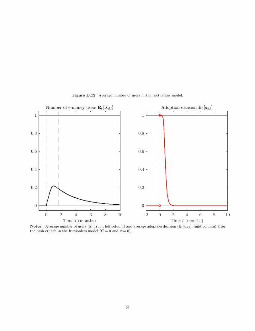
Figure D.12: Average number of users in the frictionless model.

0 2 4 6 8 10

Time t (months)

0

0.2

0.4

0.6

0.8

1

Number of e-money users Et [Xd;t]

-2 0 2 4 6 8 10

Time t (months)

0

0.2

0.4

0.6

0.8

1

Adoption decision Et [ad;t]

Notes : Average number of users (Et [Xd,t], left column) and average adoption decision (Et [ad,t], right column) afterthe cash crunch in the frictionless model (C = 0 and κ = 0).

81

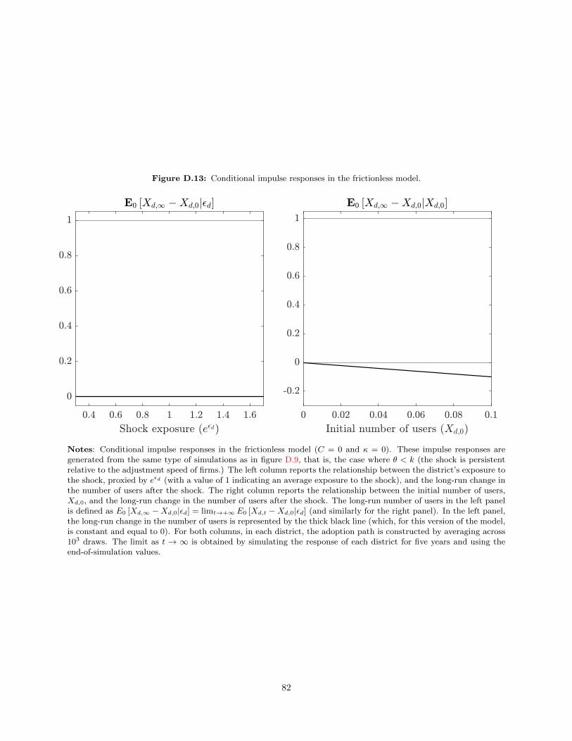
Figure D.13: Conditional impulse responses in the frictionless model.

0.4 0.6 0.8 1 1.2 1.4 1.6

Shock exposure (e0d)

0

0.2

0.4

0.6

0.8

1

E0 [Xd;1 !Xd;0j0d]

0 0.02 0.04 0.06 0.08 0.1

Initial number of users (Xd;0)

-0.2

0

0.2

0.4

0.6

0.8

1

E0 [Xd;1 !Xd;0jXd;0]

Notes: Conditional impulse responses in the frictionless model (C = 0 and κ = 0). These impulse responses aregenerated from the same type of simulations as in figure D.9, that is, the case where θ < k (the shock is persistentrelative to the adjustment speed of firms.) The left column reports the relationship between the district’s exposure tothe shock, proxied by eεd (with a value of 1 indicating an average exposure to the shock), and the long-run change inthe number of users after the shock. The right column reports the relationship between the initial number of users,Xd,0, and the long-run change in the number of users after the shock. The long-run number of users in the left panelis defined as E0 [Xd,∞ −Xd,0|εd] = limt→+∞E0 [Xd,t −Xd,0|εd] (and similarly for the right panel). In the left panel,the long-run change in the number of users is represented by the thick black line (which, for this version of the model,is constant and equal to 0). For both columns, in each district, the adoption path is constructed by averaging across103 draws. The limit as t → ∞ is obtained by simulating the response of each district for five years and using theend-of-simulation values.

82

Figure D.14: Map of the Distribution of Exposured

Notes: The figure maps the distribution of Exposured (as described in Section 2) across Indian districts. Source:Reserve Bank of India

83

Figure D.15: Distribution of Exposured across districts

01

23

4D

ensi

ty

0 .2 .4 .6 .8 1Exposure

Notes: The figure shows the distribution of Exposured (as described in Section 2) across Indian districts. Source:Reserve Bank of India.

84

Figure D.16: Distribution of growth in deposits across districts

010

2030

Den

sity

-.2 0 .2 .4Quarterly growth in deposits

Sep-Dec 2015

Sep-Dec 2016

Notes: Distribution across deposits of the growth in total banking sector deposits from October to December duringthe year 2015 (blue) and 2016 (black). The vertical dashed lines represents the corresponding mean deposit growthfor these years. Source: Reserve Bank of India.

85

Figure D.17: Robustness: one-state out

.51.

52.

53.

54.

55.

5Ef

fect

on

amou

nt tr

ansa

cted

AND

HR

A PR

ADES

H

ASSA

M

BIH

AR

CH

HAT

TISG

ARH

GO

A

GU

JAR

AT

HAR

YAN

A

HIM

ACH

AL P

RAD

ESH

JAM

MU

&KAS

HM

IR

JHAR

KHAN

D

KAR

NAT

AKA

KER

ALA

MAD

HYA

PR

ADES

H

MAH

ARAS

HTR

A

OR

ISSA

PUN

JAB

RAJ

ASTH

AN

TAM

IL N

ADU

UTT

AR P

RAD

ESH

UTT

ARAK

HAN

D

WES

T BE

NG

ALState excluded from sample

Notes: This figure reports a robustness in which we exclude from the main analysis one state at a time and werecalculate the main coefficient of interest. For the main analysis, we consider the specification in which we lookat amount of transactions as an outcome and we consider the coefficient on post multiplied to the chest exposuremeasure. Each bar reports the main coefficient for the specification excluding the state in the x-axis and the 95%confidence interval. The horizontal dashed line is the main coefficient from the main table of the paper, added forreference.

86

Figure D.18: Consumption responses based on exposure to the shock

-.4-.2

0.2

.4Ef

fect

on

tota

l con

sum

ptio

n

-3 -2 -1 0 1 2 3Survey-time

Notes: The figure plots estimates of consumption responses depending on exposure to the shock (Exposured). Thespecification we estimate is a version of equation 16 in which each coefficient is based on the interaction of thetreatment variable with a event-time dummy. We report the event-time estimates of the coefficient δ. The treatmentis our measure of Exposured as described in Section 2. The dependent variable on the y-axis is the (log) total expenseby household (as described in Section 4). 95% confidence intervals are represented with the vertical lines; standarderrors are clustered at the district level. Source: CMIE Consumption Data.

87

Figure D.19: Consumption responses based on placebo shocks

-.10

.1.2

Effe

ct o

n To

tal C

onsu

mpt

ion

Feb-15 May-15 Aug-15 Nov-15 Feb-16Placebo Survey-time

Notes: The figure plots the estimates of consumption responses depending on exposure to the shock where we assumethe occurrence of a “fake” shock in each survey-time corresponding to each entry on the x-axis. The specificationwe estimate is a version of equation 16 in which each coefficient is based on the interaction of the treatment variable(Exposured) with an event-time dummy. We report the coefficient δ for the event-time right after shock. Thetreatment variable is our measure of Exposured for the district (as described in Section 2). The dependent variablelog(yh,d,t) is the log of total consumption (as described in Section 4). 95% confidence intervals are represented withthe vertical lines; standard errors are clustered at the district level. Source: CMIE Consumption Data.

88

Table D.1: Share of Chest Banks and Deposit Growth

∆ log(deposits) ∆ log(depositsadj.) ∆ log(depositsN )

(1) (2) (3) (4) (5) (6)

Chest Exposure 0.094*** 0.083*** 0.085*** 0.075*** 1.821*** 1.621***[0.013] [0.012] [0.013] [0.012] [0.257] [0.238]

log(Pre Deposits) -0.035*** -0.035*** -0.677***[0.003] [0.003] [0.063]

% villages with ATM 0.023 0.020 0.445[0.040] [0.042] [0.769]

% villages with banks -0.051** -0.051** -1.000**[0.023] [0.024] [0.449]

Rural Pop./Total Pop. -0.063*** -0.070*** -1.224***[0.016] [0.017] [0.317]

log(population) 0.036*** 0.035*** 0.707***[0.003] [0.003] [0.068]

Observations 512 512 512 512 512 512R-squared 0.118 0.313 0.099 0.290 0.118 0.313District Controls X X X

Notes: The table reports the results from regression of the district-level deposit growth (between September 30,2016 and December 31, 2016) on the measure of Exposured for the district (as described in Section 2). Columns (1)and (2) use the measure of change in total deposits. Columns (3) and (4) uses the measure of abnormal growth intotal deposits, which adjust for the normal deposit growth by the growth in district-deposit in same quarter for thelast two years. Columns (5) and (6) uses the dependent variable of deposit growth that is normalized to have meanzero and standard deviation 1. Odd columns shows the correlation without any controls. Even columns include thedistrict-level controls for (log) pre-shock banking deposits, share of villages with ATM facilities, share of villages withbanking facility, share of rural population and level of population in the district. Robust standard errors are reportedin parentheses; ∗ ∗ ∗ : p < 0.01, ∗∗ : p < 0.05, ∗ : p < 0.1.

89

Table D.2: Exposured and Deposit Growth (pre-shock quarters)

(1) (2) (3) (4) (5) (6) (7) (8) (9) (10) (11) (12)201604 201603 201602 201601 201504 201503 201502 201501 201404 201403 201402 201401

Chest Exposure 1.621*** -0.404 0.476** 0.137 0.163 0.342 -0.040 0.315 0.345 -0.734*** 0.165 0.012[0.238] [0.260] [0.236] [0.234] [0.268] [0.255] [0.231] [0.240] [0.291] [0.280] [0.257] [0.269]

Observations 512 512 512 512 512 512 512 512 512 512 512 512R-squared 0.313 0.027 0.026 0.162 0.020 0.054 0.044 0.061 0.017 0.037 0.100 0.124District Controls X X X X X X X X X X X X

Notes: Regression of district-level deposit growth for all eleven quarters before the shock (2016 Q4) on the density of chest banks in the district. The dependentvariable is normalized to have mean zero and standard deviation 1. Treatment variable is our measure of Exposured for the district (as described in Section2). District-level controls include (log) pre-shock banking deposits, share of villages with ATM facilities, share of villages with banking facility, share of ruralpopulation and level of population in the district. Standard error in parentheses; ∗ ∗ ∗ : p < 0.01, ∗∗ : p < 0.05, ∗ : p < 0.1.

90

Table D.3: Firms adoption rates in the simulated data

No complementarities (C = 0) Complementarities (C > 0)

ρ 0.862 0.863

(0.861,0.864) (0.862,0.864)

β −0.175 −0.177

(-0.180,-0.170) (-0.183,-0.171)

γ −0.016 0.198

(-0.020,-0.011) (0.196,0.200)

Observations per simulation 2,100,000 2,100,000

Average R-sq. 0.754 0.837

Notes: This table reports the estimates of the panel data regression model 10 on simualated firm-level data. Thecoefficient ρ is the autocorrelation of a firm’s technology choice, xi,d,t, while the coefficient β captures the dependenceon the stock of money, Md,t−∆, and the coefficient γ captures the dependence on the existing share of adopters,Xd,t−∆. The simulated data is aggregated at the district level and sampled monthly; see text for details. The 95%confidence interval is reported in parentheses.

Table D.4: District adoption rates based on initial adoption in electronic payment data: OLS

log(amount) log(# users) log(# switchers)

(1) (2) (3) (4) (5) (6)

1 (Any Adopter)d × 1 (t ≥ t0) 1.416*** 1.751*** 1.312***

[0.379] [0.188] [0.150]

log(pre-amount)d × 1 (t ≥ t0) 0.050 0.173*** 0.127***

[0.050] [0.022] [0.018]

Observations 6,846 6,846 6,846 6,846 6,552 6,552

R-squared 0.849 0.848 0.880 0.878 0.842 0.839

District f.e. X X X X X X

Month f.e. X X X X X X

District Controls × Month f.e. X X X X X X

Notes: The table shows adoption dependence on initial conditions at the district level. The specification estimated isequation 8. In the first row, Id is a dummy if a district had a positive adoption level before the demonetization. In thesecond row, Id the total amount of transactions before the demonetization. In Columns (1) and (2), the dependentvariable is the log of the total amount (in Rs.) of transactions carried out using digital wallet in district d duringmonth t; in Columns (3) and (4), the dependent variable is the log of the total number of active retailers using digitalwallet in district d during month t; in Columns (5)-(6), the dependent variable is the log of the total number of newretailers joining the digital wallet in district d during month t. District-level controls include (log) pre-shock bankingdeposits, share of villages with ATM facilities, share of villages with banking facility, share of rural population andlevel of population in the district. Standard errors are clustered at the district level. ∗ ∗ ∗ : p < 0.01, ∗∗ : p < 0.05,∗ : p < 0.1.

91

Table D.5: District adoption rates based on initial adoption: Alternative specification

log(amount) log(# users) log(# switchers)

δ = 200 δ = 300 δ = 400 δ = 200 δ = 300 δ = 400 δ = 200 δ = 300 δ = 400

(1) (2) (3) (4) (5) (6) (7) (8) (9)

(Distance To Hub > δ km.) × 1t≥t0 -1.309*** -1.129*** -1.113*** -0.537*** -0.499*** -0.482*** -0.358** -0.357*** -0.360***

[0.374] [0.357] [0.345] [0.182] [0.151] [0.138] [0.143] [0.116] [0.108]

Observations 6,846 6,846 6,846 6,846 6,846 6,846 6,846 6,846 6,846

R-squared 0.886 0.886 0.886 0.912 0.912 0.912 0.871 0.871 0.871

District f.e. X X X X X X X X X

Month f.e. X X X X X X X X X

District Controls × Month f.e. X X X X X X X X X

State × Month f.e. X X X X X X X X X

Notes: The table shows difference-in-differences estimate of the effect of initial conditions, using distance to the nearest hub (defined as districts with greaterthan 500 retailers in September 2016) as a proxy for the initial share of adopters. The specification estimated is equation 9, replacing Dd with a dummy fordistance to hub based on threshold δ (1Distance To Hub>δ km.), The dependent variable is either the or the log of the total nominal value of transactions; logof total number of active firms; log of total number of new firms on the digital wallet. District-level controls include (log) pre-shock banking deposits, share ofvillages with ATM facilities, share of villages with banking facility, share of rural population, level of population, distance to state capital and employment ratein the district. Standard errors are clustered at the district level. ∗ ∗ ∗ : p < 0.01, ∗∗ : p < 0.05, ∗ : p < 0.1.

92

Table D.6: Firm adoption based on existing adoption rate (district-level)

(1) (2) (3) (4)

xi,k,d,t = log(amount)i,k,d,t

xi,k,d,t−1 0.572*** 0.474*** 0.420*** 0.410***

(0.0100) (0.0108) (0.0108) (0.0105)

Xk,d,t−1 0.0696*** 0.117*** 0.0295*** 0.00606***

(0.00257) (0.00662) (0.00439) (0.00134)

R2 0.398 0.437 0.459 0.463

xi,k,d,t = log(# transactions)i,k,d,t

xi,k,d,t−1 0.776*** 0.709*** 0.635*** 0.624***

(0.0101) (0.00933) (0.0149) (0.0148)

Xk,d,t−1 0.0237*** 0.0600** 0.116*** 0.0212***

(0.00821) (0.0301) (0.00693) (0.00205)

R2 0.598 0.615 0.635 0.637

xi,k,d,t = 1 On platformi,k,d,txi,k,d,t−1 0.528*** 0.408*** 0.378*** 0.370***

(0.00828) (0.00931) (0.00857) (0.00849)

Xk,d,t−1 0.0158*** 0.0314*** 0.0198*** 0.00489***

(0.00131) (0.00180) (0.00202) (0.000938)

R2 0.369 0.419 0.433 0.437

Firm F.E. X X X

District × Week F.E. X X

Industry × Week F.E. X

Observations 58,022,429 58,022,429 58,021,662 58,021,662

Notes: The table reports estimates of the dependence of firm-level adoption rates on the share of other adoptersin the industry/district. The specification we estimate is a version of equation 11 at district-level in which eachcoefficient is interacted with a weekly dummy; we reported estimates of the coefficient γ. The top panel reportseffects when x is the total value of transactions, the middle panel reports effects when x is the total number oftransactions, and the bottom panel reports effects when x is a dummy for whether the firm used the platform overthe past week. Standard errors are clustered at the district level. ∗ ∗ ∗ : p < 0.01, ∗∗ : p < 0.05, ∗ : p < 0.1.

93

Table D.7: Firm adoption based on existing adoption rate (allowing for spillovers across industries)

(1) (2) (3) (4)

xi,p,d,t = log(amount)i,p,d,t

xi,p,d,t−1 0.533*** 0.444*** 0.375*** 0.358***

(0.006) (0.005) (0.004) (0.003)

Xp,d,t−1 0.076*** 0.135*** 0.023*** 0.016***

(0.002) (0.002) (0.002) (0.001)

R2 0.364 0.402 0.432 0.441

xi,p,d,t = log(# transactions)i,p,d,t

xi,p,d,t−1 0.711*** 0.621*** 0.586*** 0.579***

(0.005) (0.005) (0.005) (0.005)

Xp,d,t−1 0.022*** 0.043*** 0.021*** 0.013***

(0.001) (0.001) (0.001) (0.001)

R2 0.548 0.573 0.585 0.590

xi,p,d,t = 1 On platformi,p,d,txi,p,d,t−1 0.496*** 0.381*** 0.334*** 0.323***

(0.007) (0.003) (0.003) (0.003)

Xp,d,t−1 0.035*** 0.071*** 0.027*** 0.015***

(0.002) (0.001) (0.001) (0.001)

R2 0.347 0.398 0.420 0.428

Firm F.E. X X X

Industry × Week F.E. X X

District × Week F.E. X

Observations 11,750,558 11,750,558 11,750,558 11,749,732

Notes: The table reports estimates of the dynamic specification for adoption based on : xi,p,d,t = αi + αdt +ρxi,p,d,t−1+γXp,d,t−1+εi,p,d,t allowing for spillovers across industries within the same pincode. We reported estimatesof the coefficient γ. The top panel reports effects when x is the total value of transactions, the middle panel reportseffects when x is the total number of transactions, and the bottom panel reports effects when x is a dummy for whetherthe firm used the platform over the past week. Standard errors are clustered at the pincode level. ∗ ∗ ∗ : p < 0.01,∗∗ : p < 0.05, ∗ : p < 0.1.

94

Table D.8: Consumption responses across categories based on exposure to the shock

Necessary Unnecessary Bills and Rent Food Recreation

(1) (2) (3) (4) (5)

(Exposure)d × 1(t = t1) -0.174*** -0.211** 0.250 -0.185*** -0.996**(0.0573) (0.0987) (0.268) (0.0595) (0.431)

Household f.e. X X X X XSurvey-time f.e. X X X X XDistrict Controls × Survey-time f.e. X X X X XHousehold controls × Survey-time f.e. X X X X XObservations 564,690 564,690 564,690 564,690 564,690R-squared 0.731 0.622 0.700 0.684 0.460

Notes: The table shows the difference-in-differences estimate for consumption responses across various categories foreach event-time after the demonetization shock relative the pre-period (four event-time). The specification estimatedis equation 16. The treatment variable is our measure of Exposured for the district (as described in Section 2). Thedependent variable log(yh,d,t) is either the log of consumption of necessary goods (Column (1)); the log of consumptionof unnecessary goods (Column (2)); log of expenditure on bills and rent (Column (3)); the log of expenditure onfood (Column (4)); the log of expenditure on recreation activities (Column (5)) as defined in Section 6. District-level controls include (log) pre-shock banking deposits, share of villages with ATM facilities, share of villages witha banking facility, share of rural population and level of population in the district. Household-level controls includepre-shock income and age of head of the household. Standard errors are clustered at the district level. ∗∗∗ : p < 0.01,∗∗ : p < 0.05, ∗ : p < 0.1.

95

Table D.9: Consumption responses based on alternative cutoff for exposure to the shock

log(Expense)

Total Necessary Unnecessary

(1) (2) (3)

1t=t1 × (Top 25% Exposure)d -0.0577** -0.0427* -0.0781**(0.0234) (0.0230) (0.0343)

1t=t2 × (Top 25% Exposure)d -0.0199 -0.0172 -0.0277(0.0296) (0.0266) (0.0454)

1t=t3 × (Top 25% Exposure)d 0.0146 -0.00438 0.0519(0.0370) (0.0307) (0.0533)

1t=t4 × (Top 25% Exposure)d -0.0187 -0.0588 0.0374(0.0588) (0.0580) (0.0786)

Household f.e. X X XSurvey-time f.e. X X XDistrict Controls × Survey-time f.e. X X XHousehold controls × Survey-time f.e. X X XObservations 564,690 564,690 564,690R-squared 0.706 0.731 0.622

Notes: The table shows difference-in-differences estimate for consumption responses for each event-time post thedemonetization shock relative the pre-period (four event-time). The specification estimated is equation 16. Treatmentvariable takes the value of 1 if our measure of Exposured for the district (as described in Section 2) is in the top25% value of exposure. The dependent variable log(yh,d,t) is either log of total consumption (Column (1)); log ofconsumption of necessary goods (Column (2)); log of consumption of unnecessary goods (Column (3)) as defined inSection 6. District-level controls include (log) pre-shock banking deposits, share of villages with ATM facilities, shareof villages with banking facility, share of rural population and level of population in the district. Household-levelcontrols include pre-shock income and age of head of the household. Standard errors are clustered at the districtlevel. ∗ ∗ ∗ : p < 0.01, ∗∗ : p < 0.05, ∗ : p < 0.1.

96

Table D.10: Heterogeneous consumption responses by district’s exposure to alternate payment system

Total Necessary Unnecessary

(1) (2) (3) (4) (5) (6)

1(t = t1)× (Exposure)d -0.303*** -0.298*** -0.280**(0.0771) (0.0740) (0.121)

1(t = t2)× (Exposure)d -0.177* -0.201** -0.114(0.0972) (0.0889) (0.157)

1(t = t3)× (Exposure)d 0.103 0.0199 0.275(0.131) (0.108) (0.203)

1(t = t4)× (Exposure)d 0.121 -0.124 0.445(0.212) (0.182) (0.319)

1(t = t1)× 1(ATM)d -0.118* -0.0506* -0.127** -0.0491** -0.0917 -0.0413(0.0615) (0.0298) (0.0518) (0.0241) (0.0963) (0.0463)

1(t = t2)× 1(ATM)d -0.148** -0.0535* -0.157*** -0.0528** -0.116 -0.0438(0.0663) (0.0302) (0.0584) (0.0253) (0.105) (0.0490)

1(t = t3)× 1(ATM)d -0.0431 0.0000 -0.0481 -0.0105 -0.0118 0.0356(0.0731) (0.0315) (0.0615) (0.0282) (0.118) (0.0486)

1(t = t4)× 1(ATM)d 0.117 0.0644 -0.0285 -0.00480 0.299* 0.145*(0.114) (0.0604) (0.0968) (0.0516) (0.174) (0.0864)

1(t = t1)× (Top 25% Exposure)d -0.106*** -0.104*** -0.102**(0.0318) (0.0291) (0.0510)

1(t = t2)× (Top 25% Exposure)d -0.0782** -0.0829** -0.0666(0.0375) (0.0335) (0.0609)

1(t = t3)× (Top 25% Exposure)d 0.00985 -0.0126 0.0669(0.0478) (0.0385) (0.0761)

1(t = t4)× (Top 25% Exposure)d 0.0227 -0.0993 0.211(0.0914) (0.0776) (0.137)

1(t = t1)× (Exposure)d × 1(ATM)d 0.185* 0.217** 0.129(0.102) (0.0987) (0.151)

1(t = t2)× (Exposure)d × 1(ATM)d 0.232* 0.261** 0.167(0.119) (0.112) (0.185)

1(t = t3)× (Exposure)d × 1(ATM)d 0.0744 0.0724 0.0536(0.142) (0.116) (0.226)

1(t = t4)× (Exposure)d × 1(ATM)d -0.139 0.0818 -0.454(0.218) (0.202) (0.326)

1(t = t1)× (Top 25% Exposure)d × 1(ATM)d 0.0913** 0.114*** 0.0479(0.0437) (0.0423) (0.0645)

1(t = t2)× (Top 25% Exposure)d × 1(ATM)d 0.101* 0.116** 0.0628(0.0520) (0.0470) (0.0811)

1(t = t3)× (Top 25% Exposure)d × 1(ATM)d 0.00388 0.0110 -0.0363(0.0600) (0.0494) (0.0933)

1(t = t4)× (Top 25% Exposure)d × 1(ATM)d -0.0622 0.0771 -0.289*(0.0994) (0.0949) (0.148)

Observations 554,894 554,894 554,899 554,899 554,899 554,899R-squared 0.704 0.704 0.730 0.730 0.618 0.618

Notes: The table shows triple-difference estimate for consumption responses for each event-time post the demoneti-zation shock relative the pre-period (four event-time), based on district’s access to ATM facility. Treatment variableis our measure of Exposured for the district (odd columns) and takes the values of 1 if the measure of Exposuredis in the top quartile of the distribution (even columns). 1(ATM)d takes the values of 1 if the number of ATM percapita in district is above the median of the distribution. The dependent variable log(yh,d,t) is either the log of totalconsumption (Column 1-2); log of necessary consumption (Column 3-4); log of unnecessary consumption (Column5-6). as defined in Section 6. District-level controls include (log) pre-shock banking deposits, share of villages withATM facilities, share of villages with banking facility, share of rural population and level of population in the district.Household-level controls include pre-shock income and age of head of the household. Standard errors are clusteredat the district level. ∗ ∗ ∗ : p < 0.01, ∗∗ : p < 0.05, ∗ : p < 0.1.

97