Shoreline Evolution:

City of Suffolk, Virginia

James River, Nansemond River, and

Chuckatuck Creek Shorelines

December 2010

Virginia Institute of Marine Science

College of William & Mary

Gloucester Point, Virginia

Shoreline Evolution: City of Suffolk, Virginia

James River, Nansemond River, and Chuckatuck Creek Shorelines

Data Report

Donna A. MilliganChristine WilcoxKevin P. O’Brien

C. Scott Hardaway, Jr.

Shoreline StudiesDepartment of Physical Sciences

Virginia Institute of Marine ScienceCollege of William & MaryGloucester Point, Virginia

This project was funded by the Virginia Coastal Zone Management Program at the Department ofEnvironmental Quality through Grant #NA09NOS4190163 of the U.S. Department of Commerce,

National Oceanic and Atmospheric Administration, under the Coastal Zone Management Act of 1972, asamended. The views expressed herein are those of the authors and do not necessarily reflect the views of

the U.S. Department of Commerce, NOAA, or any of its subagencies.

December 2010

i

Table of Contents

Table of Contents . . . . . . . . . . . . . . . . . . . . . . . . . . . . . . . . . . . . . . . . . . . . . . . . . . . . . . . . . . . . . . i

List of Figures . . . . . . . . . . . . . . . . . . . . . . . . . . . . . . . . . . . . . . . . . . . . . . . . . . . . . . . . . . . . . . . ii

List of Tables . . . . . . . . . . . . . . . . . . . . . . . . . . . . . . . . . . . . . . . . . . . . . . . . . . . . . . . . . . . . . . . . ii

1 Introduction . . . . . . . . . . . . . . . . . . . . . . . . . . . . . . . . . . . . . . . . . . . . . . . . . . . . . . . . . . 1

2 S hore Settings . . . . . . . . . . . . . . . . . . . . . . . . . . . . . . . . . . . . . . . . . . . . . . . . . . . . . . . . . . 12.1 Physical Setting . . . . . . . . . . . . . . . . . . . . . . . . . . . . . . . . . . . . . . . . . . . . . . . . . . . . . . 12.2 Hydrodynamic Setting . . . . . . . . . . . . . . . . . . . . . . . . . . . . . . . . . . . . . . . . . . . . . . . . 4

3 Methods . . . . . . . . . . . . . . . . . . . . . . . . . . . . . . . . . . . . . . . . . . . . . . . . . . . . . . . . . . . . . . 73.1 Photo Rectification and Shoreline Digitizing . . . . . . . . . . . . . . . . . . . . . . . . . . . . . . . 73.2 Rate of Change Analysis . . . . . . . . . . . . . . . . . . . . . . . . . . . . . . . . . . . . . . . . . . . . . . . 8

4 Results and Discussion . . . . . . . . . . . . . . . . . . . . . . . . . . . . . . . . . . . . . . . . . . . . . . . . . . . 9

5 S ummary . . . . . . . . . . . . . . . . . . . . . . . . . . . . . . . . . . . . . . . . . . . . . . . . . . . . . . . . . . . . 11

6 R eferences . . . . . . . . . . . . . . . . . . . . . . . . . . . . . . . . . . . . . . . . . . . . . . . . . . . . . . . . . . . . 12

Appendix A. End Point Rate of Shoreline Change Maps

Appendix B. Historical Shoreline Photo Maps

ii

List of Figures

Figure 1. Location City of Suffolk within the Chesapeake Bay Estuarine System . . . . . . . . . . . 2Figure 2. Geologic map of City of Suffolk (from Mixon et al., 1989) . . . . . . . . . . . . . . . . . . . . 3Figure 3. Index of shoreline plates. . . . . . . . . . . . . . . . . . . . . . . . . . . . . . . . . . . . . . . . . . . . . . . . . 5

List of Tables

Table 1. Summary wind conditions at Norfolk International Airport from 1960-1990 . . . . . . . . 6Table 2. Suffolk shore segments and their average rate of change for various time

periods . . . . . . . . . . . . . . . . . . . . . . . . . . . . . . . . . . . . . . . . . . . . . . . . . . . . . . . . . . . . . . . 10

1

1 Introduction

Shoreline evolution is the change in the shore zone through time. Along ChesapeakeBay’s estuarine shores, it is a process and response system. The processes at work includewinds, waves, tides and currents which shape and modify coastlines by eroding, transporting anddepositing sediments. The shore line is commonly plotted and measured to provide a rate ofchange, but it is as important to understand the geomorphic patterns of change. Shore analysisprovides the basis to know how a particular coast has changed through time and how it mightproceed in the future.

The purpose of this data report is to document how the shore zone of Suffolk (Figure 1)has evolved since 1937. Aerial imagery was taken for most of the Bay region beginning thatyear and can be used to assess the geomorphic nature of shore change. Aerial photos show howthe coast has changed, how beaches, dunes, bars, and spits have grown or decayed, how barriershave breached, how inlets have changed course, and how one shore type has displaced another orhas not changed at all. Shore change is a natural process but, quite often, the impacts of man,through shore hardening or inlet stabilization, come to dominate a given shore reach. In additionto documenting historical shorelines, the change in shore positions along the rivers and largercreeks in the City of Suffolk will be quantified in this report. The shorelines of very irregularcoasts, small creeks around inlets, and other complicated areas, will be shown but not quantified.

2 Shore Settings

2.1 Physical Setting

City of Suffolk is located east of Virginia’s Southside and has about 113 miles of tidalshoreline on several bodies water including James River, Nansemond River, and ChuckatuckCreek. When all creeks and rivers that drain into these bodies of water are included, these areashave about 10 miles, 78 miles, and 25 miles, respectively (CCRM, 1976). The historic rate ofchange along the James River was 2.3 -ft/yr, and along the western shore of the mouth of theNansemond River, the rate varied between -1.2 ft/yr and -2.9 ft/yr (Byrne and Anderson, 1978).

The coastal geomorphology of the City is a function of the underlying geology and thehydrodynamic forces operating across the land/water interface, the shoreline (Figure 2). TheAtlantic Ocean has come and gone numerous times over the Virginia coastal plain over the pastmillion years. The effect has been to rework older deposits into beach and lagoonal deposits atthe time of the transgressions. The topography of Suffolk is a result of these changes inshoreline. The majority of the City consists of the Lynnhaven Member of Tabb Formationwhich was deposited during the last high stand of sea level 135,000-80,000 years before present.The last low stand of sea level found the ocean coast about 60 miles to the east when sea levelabout 400 feet lower than today and the coastal plain was broad and low (Toscano, 1992). Thislow-stand occurred about 18,000 years ago during the last glacial maximum.

Figure 1. Location City of Suffolk within the Chesapeake Bay Estuarine System

Windsor Formation (lower Pleistocene or upper Pliocene) - Gray and yellow to reddish-brown sand, gravel, silt,and clay. Constitutes surficial deposits if extensive plain (alt. 85-95 ft) seaward of Surry scarp and coeval, fluvial-estuarine terrace west of scarp. Unit is 0-40 ft thick.

Chuckatuck formation (middle (?) Pleistocene) - Light- to medium-gray, yellowish-orange, and reddish-brownsand. silt and clay and minor amounts of dark-brown and brownish-black peat. Unit is 0 - 26 ft thick.

Shirley Formation (middle Pleistocene) - Light-to dark-gray and brown sand, gravel, silt, clay, and peat. Thickness is 0-80 ft.

Charles City Formation (lower Pleistocene (?)) - Light- to medium-gray and light- to dark- yellowish and reddish- brownsand, silt, and clay composing surficial deposits of riverine terrace and coast-parallel plains at altitudes of 70-80 ft. Unit is0-55ft or more in thickness.

Figure 2. Geologic map of City of Suffolk (from Mixon et al., 1989)

Sedgefield Member of Tabb Formation - Pebbly to bouldery, clayey sand and fine to medium, shelly sand grading upwardto sandy and clayey silt. Unit constitutes surficial deposit of river- and coast parallel plains (alt. 20-30ft) bounded onLandward side by Suffolk and Harpersville scarps. Thickness is 0-50 ft.

Alluvium - Fine to coarse gravelly sand and sandy gravel, silt, and clay, light- to medium- gray and yellowish-gray. MostlyHolocene but, locally, includes low-lying Pleistocene(?) Terrace deposits. As much as 80 ft thick along major streams.

Lynnhaven Member of - Pebbly and cobbly, fine to coarse gray sand grading upward into clayey and siltyfine sand and sandy silt; locally, at base of unit, medium to coarse crossbedded sand and clayey silt containing abundantPlant material fill channels cut into underlying stratigraphic units. Thickness is 0-20 ft.

Tabb Formation

Artificial Fill - Areas filled for construction and waste disposal.

Swap deposits - Reddish-brown fibrous peat, brown to black sapric peat, and peaty mud and sand. Thickness generally lessthan 10 ft.

Dune Sand - White to light-yellowish-gray, fine to medium, well sorted, massive to crosslaminated. Thickness is 0-15ft.

Miles0 2 4

4

As sea level began to rise and the coastal plain watersheds began to flood, shorelinesbegan to recede. The slow rise in sea level is one of two primary long-term processes whichcause the shoreline to recede; the other is wave action, particularly during storms. As shorelinesrecede or erode the bank material provides the sands for the offshore bars, beaches and dunes.

Sea level rise has been well documented in the Tidewater Region. Tide data collected atSewells Point in Norfolk (Figure 1) show that sea level has risen 0.17 inches/yr or 1.45 ft/century(http://www.co-ops.nos.noaa.gov/). This directly effects the reach of storms and their impact onshorelines. Anecdotal evidence of storm surge during Hurricane Isabel, which impacted NorthCarolina and Virginia on September 18, 2003, put it on par with the storm surge from the “stormof the century” which impacted the lower Chesapeake Bay in August 1933. Boon (2003)showed that even though the tides during the storms were very similar, the difference being only1.5 inches, the amount of surge was different. The 1933 storm produced a storm surge that wasgreater than Isabel’s by slightly more than a foot. However, analysis of the mean water levelsfor the months of both August 1933 and September 2003 showed that sea level has risen by 1.35ft at Hampton Roads in the seventy years between these two storms (Boon, 2003). This is theapproximate time span between our earliest aerial imagery (1937) and our most recent (2009)which means the impact of sea level rise to shore change is significant.

2.2 Hydrodynamic Setting

Tide range for Suffolk is 2.4 ft for the mean tidal range and 2.8 ft for the spring tidalrange at Sewells Point located at the Norfolk U.S. Naval Station at Hampton Roads. At theentrance to Chuckatuck Creek, tide range is 2.8 ft (3.4 ft spring range) (NOAA, 2007).

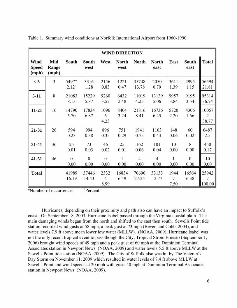
Wind data from Norfolk International Airport reflect the frequency and speeds of windoccurrences from 1960 to 1990 (Table 1). These data provide a summary of winds possiblyavailable to generate waves. Winds from the north and south have the largest frequency ofoccurrence, but the north and northeast have the highest occurrence of large winds that willgenerate large waves. Generally, the James River and upper Nansemond River shorelines aresubject to a larger wave climate due to greater fetch opportunities. The more protected creekshave a less energetic wave climate.

Figure 3. Index of shoreline plates.

6

Table 1. Summary wind conditions at Norfolk International Airport from 1960-1990.

WIND DIRECTION

Wind Speed(mph)

MidRange(mph)

South Southwest

West Northwest

North Northeast

East Southeast

Total

< 5 3 5497*2.12+

33161.28

21560.83

12210.47

3574813.78

20500.79

36111.39

29951.15

5659421.81

5-11 8 210838.13

152295.87

92603.57

64322.48

110194.25

131395.06

99573.84

91953.54

9531436.74

11-21 16 147905.70

178346.87

10966

4.23

84043.24

218168.41

167366.45

57202.20

43061.66

100572

38.77

21-31 26 5940.23

9940.38

8960.35

7510.29

19410.75

11030.43

1480.06

600.02

64872.5

31-41 36 250.01

730.03

460.02

250.01

1620.06

1010.04

100.00

80.00

4500.17

41-51 46 00.00

00.00

00.00

10.00

40.00

40.00

10.00

00.00

100.00

Total 4198916.19

3744614.43

23324

8.99

168346.49

7069027.25

3313312.77

19447

7.50

165646.38

259427

100.00*Number of occurrences +Percent

Hurricanes, depending on their proximity and path also can have an impact to Suffolk’scoast. On September 18, 2003, Hurricane Isabel passed through the Virginia coastal plain. Themain damaging winds began from the north and shifted to the east then south. Sewells Point tidestation recorded wind gusts at 58 mph, a peak gust at 73 mph (Beven and Cobb, 2004), and water levels 7.9 ft above mean lower low water (MLLW). (NOAA, 2009). Hurricane Isabel wasnot the only recent tropical event to pass though the City; Tropical Strom Ernesto (September 1,2006) brought wind speeds of 49 mph and a peak gust of 60 mph at the Dominion TerminalAssociates station in Newport News (NOAA, 2009) and water levels 5.5 ft above MLLW at theSewells Point tide station (NOAA, 2009). The City of Suffolk also was hit by The Veteran’sDay Storm on November 11, 2009 which resulted in water levels of 7.4 ft above MLLW atSewells Point and wind speeds at 20 mph with gusts 40 mph at Dominion Terminal Associatesstation in Newport News (NOAA, 2009).

7

3 Methods

3.1 Photo Rectification and Shoreline Digitizing

An analysis of aerial photographs provides the historical data necessary to understandthe suite of processes that work to alter a shoreline. Images of the Suffolk Shoreline from 1937,1954, 1963, 1994, 2002, 2007 and 2009 were used in the analysis The 1994, 2002, 2007 and2009 images were available from other sources. The 1994 imagery was orthorectified by theU.S. Geological Survey (USGS) and the 2002, 2007 and 2009 imagery was orthorectified by theVirginia Base Mapping Program (VBMP). The 1937, 1954, and 1963 photos were a part of theVIMS Shoreline Studies Program archives. The entire shoreline generally was not flown in asingle day. The dates for each year are: 1937- April 17, May 20, and September 4; 1954- June 3and October 13; 1963- February 18. We could not ascertain the exact dates the 1994 images wereflown, but the 2002, 2007, and 2009 were all flown in February of their respective years.

The 1937, 1954, and 1963 images were scanned as tiffs at 600 dpi and converted toERDAS IMAGINE (.img) format. These aerial photographs were orthographically corrected toproduce a seamless series of aerial mosaics following a set of standard operating procedures. The1994 Digital Orthophoto Quarter Quadrangles (DOQQ) from USGS were used as the referenceimages. The 1994 photos are used rather than higher quality, later photos because of thedifficulty in finding control points that match the earliest 1937 images.

ERDAS Orthobase image processing software was used to orthographically correct theindividual flight lines using a bundle block solution. Camera lens calibration data were matchedto the image location of fiducial points to define the interior camera model. Control points from1994 USGS DOQQ images provide the exterior control, which is enhanced by a large number ofimage-matching tie points produced automatically by the software. The exterior and interiormodels were combined with a digital elevation model (DEM) from the USGS National ElevationDataset to produce an orthophoto for each aerial photograph. The orthophotographs wereadjusted to approximately uniform brightness and contrast and were mosaicked together usingthe ERDAS Imagine mosaic tool to produce a one-meter resolution mosaic .img format. Tomaintain an accurate match with the reference images, it is necessary to distribute the controlpoints evenly, when possible. This can be challenging in areas with lack of ground features,poor photo quality and lack of control points. Good examples of control points were manmadefeatures such as road intersections and stable natural landmarks such as ponds and creeks thathave not changed much over time. The base of tall features such as buildings, poles, or trees canbe used, but the base can be obscured by other features or shadows making these locationsdifficult to use accurately. Some areas of the City were particularly difficult to rectify due to thelack of development when compared to the reference images. Some areas of the original photoswere “whited-out”due to the sensitive nature of certain installations at that time.

Once the aerial photos were orthorectified and mosaicked, the shorelines were digitizedin ArcMap with the mosaics in the background. The morphologic toe of the beach or edge of

8

marsh was used to approximate low water. High water or limit of runup is difficult to determineon much of the shoreline due to narrow or non-existent beaches against upland banks orvegetated cover. In areas where the shoreline was not clearly identifiable on the aerialphotography, the location was estimated based on the experience of the digitizer. The displayedshorelines are in shapefile format. One shapefile was produced for each year that wasmosaicked.

Horizontal positional accuracy is based upon orthorectification of scanned aerialphotography against the USGS digital orthophoto quadrangles. To get vertical control, the USGS30m DEM data was used. The 1994 USGS reference images were developed in accordance withNational Map Accuracy Standards (NMAS) for Spatial Data Accuracy at the 1:12,000 scale. The 2002, 2007 and 2009 Virginia Base Mapping Program’s orthophotography were developed inaccordance with the National Standard for Spatial Data Accuracy (NSSDA). Horizontal rootmean square error (RMSE) for historical mosaics was held to less than 20 ft.

Using methodology reported in Morton et al. (2004) and National Spatial DataInfrastructure (1998), estimates of error in orthorectification, control source, DEM and digitizingwere combined to provide an estimate of total maximum shoreline position error. The data setsthat were orthorectified (1937, 1954, and 1963) have an estimated total maximum shorelineposition error of 20.0 ft, while the total maximum shoreline error for the four existing datasetsare estimated at 18.3 ft for USGS and 10.2 ft for VBMP. The maximum annualized error forthe shoreline data is +0.7 ft/yr. The smaller rivers and creeks are more prone to error due to theirgeneral lack of good control points for photo rectification, narrower shore features, tree andground cover and overall smaller rates of change. For these reasons, some areas were onlydigitized in 1937 and 2009. It was decided that digitizing the intervening years would introducesmore errors rather then provide additional information.

3.2 Rate of Change Analysis

The Digital Shoreline Analysis System (DSAS) was used to determine the rate of changefor the City’s shoreline (Himmelstoss, 2009). All DSAS input data must be managed within apersonal geodatabase, which includes all the baselines for Suffolk and the digitized shorelinesfor 1937, 1954, 1963, 1994, 2002, 2007, and 2009. Baselines were created about 200 feet orless, depending on features and space, seaward of the 1937 shoreline and encompassed most ofthe City’s main shorelines but generally did not include the smaller creeks. It also did notinclude areas that have unique shoreline morphology such as creek mouths and spits. DSASgenerated transects perpendicular to the baseline about 33 ft apart. For Suffolk, this methodrepresented about 37 miles of shoreline along 5,960 transects.

The End Point Rate (EPR) is calculated by determining the distance between the oldestand most recent shoreline in the data and dividing it by the number of years between them. Thismethod provides an accurate net rate of change over the long term and is relatively easy to applyto most shorelines since it only requires two dates. This method does not use the interveningshorelines so it may not account for changes in accretion or erosion rates that may occur through

9

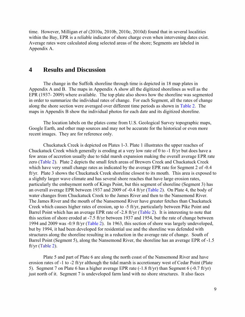
time. However, Milligan et al (2010a, 2010b, 2010c, 2010d) found that in several localitieswithin the Bay, EPR is a reliable indicator of shore charge even when intervening dates exist.Average rates were calculated along selected areas of the shore; Segments are labeled inAppendix A.

4 Results and Discussion

The change in the Suffolk shoreline through time is depicted in 18 map plates inAppendix A and B. The maps in Appendix A show all the digitized shorelines as well as theEPR (1937- 2009) where available. The top plate also shows how the shoreline was segmentedin order to summarize the individual rates of change. For each Segment, all the rates of changealong the shore section were averaged over different time periods as shown in Table 2. Themaps in Appendix B show the individual photos for each date and its digitized shoreline.

The location labels on the plates come from U.S. Geological Survey topographic maps,Google Earth, and other map sources and may not be accurate for the historical or even morerecent images. They are for reference only.

Chuckatuck Creek is depicted on Plates 1-3. Plate 1 illustrates the upper reaches ofChuckatuck Creek which generally is eroding at a very low rate of 0 to -1 ft/yr but does have afew areas of accretion usually due to tidal marsh expansion making the overall average EPR ratezero (Table 2). Plate 2 depicts the small fetch areas of Brewers Creek and Chuckatuck Creekwhich have very small change rates as indicated by the average EPR rate for Segment 2 of -0.4ft/yr. Plate 3 shows the Chuckatuck Creek shoreline closest to its mouth. This area is exposed toa slightly larger wave climate and has several shore reaches that have large erosion rates,particularly the embayment north of Kings Point, but this segment of shoreline (Segment 3) hasan overall average EPR between 1937 and 2009 of -0.4 ft/yr (Table 2). On Plate 4, the body ofwater changes from Chuckatuck Creek to the James River and then to the Nansemond River. The James River and the mouth of the Nansemond River have greater fetches than ChuckatuckCreek which causes higher rates of erosion, up to -5 ft/yr, particularly between Pike Point andBarrel Point which has an average EPR rate of -2.8 ft/yr (Table 2). It is interesting to note thatthis section of shore eroded at -7.5 ft/yr between 1937 and 1954, but the rate of change between1994 and 2009 was -0.9 ft/yr (Table 2). In 1963, this section of shore was largely undeveloped,but by 1994, it had been developed for residential use and the shoreline was defended withstructures along the shoreline resulting in a reduction in the average rate of change. South ofBarrel Point (Segment 5), along the Nansemond River, the shoreline has an average EPR of -1.5ft/yr (Table 2).

Plate 5 and part of Plate 6 are along the north coast of the Nansemond River and haveerosion rates of -1 to -2 ft/yr although the tidal marsh is accretionary west of Cedar Point (Plate5). Segment 7 on Plate 6 has a higher average EPR rate (-1.8 ft/yr) than Segment 6 (-0.7 ft/yr)just north of it. Segment 7 is undeveloped farm land with no shore structures. It also faces

10

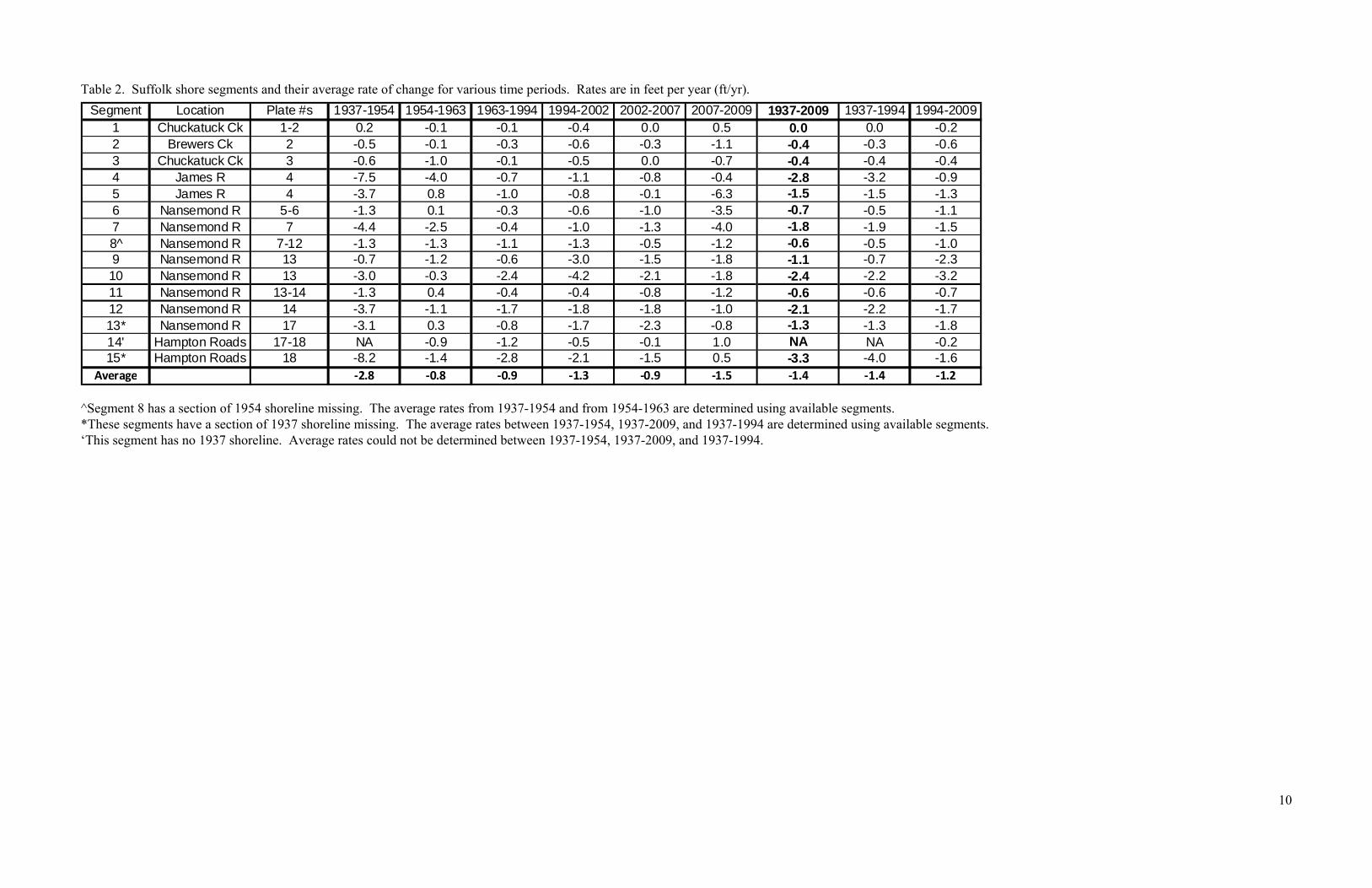
Table 2. Suffolk shore segments and their average rate of change for various time periods. Rates are in feet per year (ft/yr).

^Segment 8 has a section of 1954 shoreline missing. The average rates from 1937-1954 and from 1954-1963 are determined using available segments.*These segments have a section of 1937 shoreline missing. The average rates between 1937-1954, 1937-2009, and 1937-1994 are determined using available segments.‘This segment has no 1937 shoreline. Average rates could not be determined between 1937-1954, 1937-2009, and 1937-1994.

Segment Location Plate #s 1937-1954 1954-1963 1963-1994 1994-2002 2002-2007 2007-2009 1937-2009 1937-1994 1994-20091 Chuckatuck Ck 1-2 0.2 -0.1 -0.1 -0.4 0.0 0.5 0.0 0.0 -0.22 Brewers Ck 2 -0.5 -0.1 -0.3 -0.6 -0.3 -1.1 -0.4 -0.3 -0.63 Chuckatuck Ck 3 -0.6 -1.0 -0.1 -0.5 0.0 -0.7 -0.4 -0.4 -0.44 James R 4 -7.5 -4.0 -0.7 -1.1 -0.8 -0.4 -2.8 -3.2 -0.95 James R 4 -3.7 0.8 -1.0 -0.8 -0.1 -6.3 -1.5 -1.5 -1.36 Nansemond R 5-6 -1.3 0.1 -0.3 -0.6 -1.0 -3.5 -0.7 -0.5 -1.17 Nansemond R 7 -4.4 -2.5 -0.4 -1.0 -1.3 -4.0 -1.8 -1.9 -1.58^ Nansemond R 7-12 -1.3 -1.3 -1.1 -1.3 -0.5 -1.2 -0.6 -0.5 -1.09 Nansemond R 13 -0.7 -1.2 -0.6 -3.0 -1.5 -1.8 -1.1 -0.7 -2.310 Nansemond R 13 -3.0 -0.3 -2.4 -4.2 -2.1 -1.8 -2.4 -2.2 -3.211 Nansemond R 13-14 -1.3 0.4 -0.4 -0.4 -0.8 -1.2 -0.6 -0.6 -0.712 Nansemond R 14 -3.7 -1.1 -1.7 -1.8 -1.8 -1.0 -2.1 -2.2 -1.713* Nansemond R 17 -3.1 0.3 -0.8 -1.7 -2.3 -0.8 -1.3 -1.3 -1.814' Hampton Roads 17-18 NA -0.9 -1.2 -0.5 -0.1 1.0 NA NA -0.215* Hampton Roads 18 -8.2 -1.4 -2.8 -2.1 -1.5 0.5 -3.3 -4.0 -1.6

Average ‐2.8 ‐0.8 ‐0.9 ‐1.3 ‐0.9 ‐1.5 ‐1.4 ‐1.4 ‐1.2

11

northeast and likely is impacted by the larger, northeast storm waves coming into theNansemond River.

Plates 7-12 include the lower reaches of the Nansemond River. The entire Segment 8 hasan average EPR rate of -0.6 ft/yr (Table 2), but varies significantly in several areas. AbrahamPoint and the unnamed island in the middle of the River on Plate 9 and Glebe Point on Plate11are accretionary due to tidal marsh expansion. Plate 11 and 12 have areas of medium to higherosion particularly due to erosion of marsh shoreline southwest Sleepy Hole Point and in WillsCove. Olds Cove on Plate 13, Segment 10 has an average EPR rate of -2.4 ft/yr. Plate 14 hasshows a large section of Knotts Neck, Segment 12, is eroding at -2.1 ft/yr (Table 2). In fact, twobreakwaters have been built along the shore where the farm field is eroding at rates up to -5 ft/yr.

Plates 15 and 16 show Bennett Creek and Knotts Creek which generally are slightlyerosional, but shore erosion rates have not been determined. Plate 17 depicts the shoreline at themouth of the Nansemond River. The shore along Segment 13 has an average EPR rate of -1.3ft/yr. A section of shore on Plates 17 and 18 was whited out on the 1937 photos. The EPR rateshown on the plates was calculated between 1954 and 2009. The section of shore near theMonitor-Merrimac Bridge Tunnel has erosion rates greater than -5 ft/yr as does a section ofshoreline at the easternmost boundary of the City.

5 Summary

Shoreline change rates vary around the City of Suffolk. Generally, the subreaches withsmaller fetches have smaller rates of change. Fetch is greater than on the James River than theNansemond River and Chuckatuck Creek, thus has greater rates of erosion. Structures builtalong the shoreline influence the more recent rates of change.

12

6 References

Beven, J. and H. Cobb, 2004. Tropical Cyclone Report Hurricane Isabel. National HurricaneCenter. National Weather Service. http://www.nhc.noaa.gov/2003isabel.shtml.

Boon, J., 2003. The Three Faces of Isabel: Storm Surge, Storm Tide, and Sea Level Rise. Informal paper. http://www.vims.edu/physical/research/isabel/.

Byrne, R.J. and G.L. Anderson, 1978. Shoreline Erosion in Tidewater Virginia. VirginiaInstitute of Marine Science. College of William & Mary, Gloucester Point, VA.

Center for Coastal Resources Management, 2008 City of Portsmouth - Shoreline InventoryReport. Virginia Institute of Marine Science. College of William & Mary, GloucesterPoint, VA.

Himmelstoss, E.A., 2009. “DSAS 4.0 Installation Instructions and User Guide” in: Thieler, E.R.,Himmelstoss, E.A., Zichichi, J.L., and Ergul, Ayhan. 2009 Digital Shoreline AnalysisSystem (DSAS) version 4.0 — An ArcGIS extension for calculating shoreline change:U.S. Geological Survey Open-File Report 2008-1278.

Milligan, D. A., K.P. O’Brien, C. Wilcox, C. S. Hardaway, JR, 2010a. Shoreline Evolution: Cityof Newport News, Virginia James River and Hampton Roads Shorelines. VirginiaInstitute of Marine Science. College of William & Mary, Gloucester Point, VA.http://web.vims.edu/physical/research/shoreline/docs/dune_evolution/NewportNews/1NewportNews_Shore_Evolve.pdf

Milligan, D. A., K.P. O’Brien, C. Wilcox, C. S. Hardaway, JR, 2010b. Shoreline Evolution: Cityof Poquoson, Virginia, Poquoson River, Chesapeake Bay, and Back River Shorelines. Virginia Institute of Marine Science. College of William & Mary, Gloucester Point, VA.http://web.vims.edu/physical/research/shoreline/docs/dune_evolution/Poquoson/1Poquoson_Shore_Evolve.pdf

Milligan, D. A., K.P. O’Brien, C. Wilcox, C. S. Hardaway, JR, 2010c. Gloucester County,Virginia York River, Mobjack Bay, and Piankatank River Shorelines. Virginia Instituteof Marine Science. College of William & Mary, Gloucester Point, VA. http://web.vims.edu/physical/research/shoreline/docs/dune_evolution/Gloucester/1Gloucester_Shore_Evolve.pdf

Milligan, D. A., K.P. O’Brien, C. Wilcox, C. S. Hardaway, JR, 2010d. Shoreline Evolution:York County, Virginia York River, Chesapeake Bay and Poquoson River Shorelines.Virginia Institute of Marine Science. College of William & Mary, Gloucester Point, VA.http://web.vims.edu/physical/research/shoreline/docs/dune_evolution/York/1York_Shore_Evolve.pdf

13

Mixon, R.B., D.S. Powars, L.W. Ward, and G.W. Andrews, 1989. Lithostratigraphy andmolluscan and diatom biostratigraphy of the Haynesville Cores, northeastern VirginiaCoastal Plain. Chapter A in Mixon, RB., ed., Geology and paleontology of theHaynessville cores, Richmond County, northeastern Virginia Coastal Plain: U.S.Geological Survey Professional Survey Professional Paper. 1489.

Morton, R.A., T.L. Miller, and L.J. Moore, 2004. National Assessment of Shoreline Change:Part 1 Historical Shoreline Change and Associated Coastal Land Loss along the U.S.Gulf of Mexico. U.S. Department of the Interior, U.S. Geological Survey Open-FileReport 2004-1043, 45 p.

National Oceanic and Atmospheric Administration, 2009. Tides and Currents.http://tidesandcurrents.noaa.gov/

National Spatial Data Infrastructure, 1998. Geospatial Positional Accuracy Standards, Part 3:National Standard for Spatial Data Accuracy. Subcommittee for Base Cartographic Data.Federal Geographic Data Committee. Reston, VA.

Toscano, M.A., 1992. Record of oxygen-isotope stage 5 on the Maryland inner shelf andAtlantic Coastal Plain – Post-transgressive-highstand regime. In Fletcher, C.H., III, andJ. F. Wehmiller (eds.), Quaternary Coasts of the United States: Marine and LacustrineSystems, SEPM Special Publication No. 48. p89-99.

Appendix AEnd Point Rate of Shoreline Change Maps

Plate 1 Plate 7 Plate 13Plate 2 Plate 8 Plate 14Plate 3 Plate 9 Plate 15Plate 4 Plate 10 Plate 16Plate 5 Plate 11 Plate 17Plate 6 Plate 12 Plate 18

Appendix BHistorical Shoreline Photo Maps

Plate 1 Plate 7 Plate 13Plate 2 Plate 8 Plate 14Plate 3 Plate 9 Plate 15Plate 4 Plate 10 Plate 16Plate 5 Plate 11 Plate 17Plate 6 Plate 12 Plate 18