Short and Simple Cycle Separators in Planar Graphs

Eli Fox-Epstein∗ Shay Mozes † Phitchaya Mangpo Phothilimthana ‡

Christian Sommer §

Abstract

We provide an implementation of an algorithm that,given a triangulated planar graph with m edges, returnsa simple cycle that is a 2/3–balanced separator consist-ing of at most

√8m edges. An efficient construction of a

short and balanced separator that forms a simple cycleis essential in numerous planar graph algorithms, e.g.,for computing shortest paths, minimum cuts, or max-imum flows. To the best of our knowledge, this is thefirst implementation of such a cycle separator algorithmwith a worst-case guarantee on the cycle length.

We evaluate the performance of our algorithm andcompare it to the planar separator algorithms recentlystudied by Holzer et al. [ESA 2005, ACM Journal of Ex-perimental Algorithms 2009]. Out of these algorithms,only the Fundamental Cycle Separator (FCS) producesa simple cycle separator. However, FCS does not pro-vide a worst-case size guarantee. We demonstrate that(i) our algorithm is competitive across all test cases interms of running time, balance and cycle length, (ii) itprovides worst-case guarantees on the cycle length, sig-nificantly outperforming FCS on some instances, and(iii) it scales to large graphs.

1 Introduction

Separators identify structure in a graph by cleavingit into two balanced parts with little mutual interfer-ence. A separator theorem typically provides worst-case guarantees on the balance of the parts and on thesize of their shared boundary. Separators have beenstudied extensively and separator theorems have beenfound for planar graphs [37, 29, 10, 31, 16, 36, 12],bounded-genus graphs [11, 17, 24], minor-free graphs[3, 34, 35, 4, 23, 40], and others.

Efficient algorithms for these graph classes often ex-ploit the fact that the input graph has small separa-tors. For example, divide-and-conquer algorithms rely

∗Tufts University, ef@cs.tufts.edu†MIT, shaym@mit.edu; part of this work was conducted while

SM was with Brown University.‡MIT, mangpo@csail.mit.edu§csom@csail.mit.edu

on decomposing a problem into subproblems with lit-tle interference. More formally, a separator of a graphG = (V,E) is a subset S ⊆ V that partitions V \ Sinto two sets A,B ⊆ V of approximately equal size1

(say |A|, |B| ≤ 2|V |/3) and no edges between the twoparts (E ∩ A × B = ∅). A smaller set S often impliesfaster algorithms providing solutions for various prob-lems such as exact shortest paths [15, 19] or approxi-mate vertex cover [30], and many more [18, 27, 13, 33,6, 22, 32, 21, 28, 5]. For planar graphs, it is knownthat |S| = O(

√|V |) is possible, even for worst-case in-

stances [29].Separators in planar graphs are based on fundamen-

tal cycles. For a spanning tree T , the fundamental cycleCuv induced by an edge uv /∈ T is the simple cycleformed by uv and the u-to-v path in T . Every funda-mental cycle C separates the graph into two parts: thesubgraph enclosed by C and the subgraph not enclosedby C. An elementary argument shows that, if the graphis triangulated, then there always exists an edge e /∈ Tsuch that Ce is a balanced separator in G. Namely,each of the two parts consists of at most 2|V |/3 vertices.A key observation is that, starting with a breadth-firstsearch tree, the size of any fundamental cycle is at mostone plus the diameter of the graph. Therefore, if thediameter is small, the simple Fundamental Cycle Sepa-rator Algorithm works well: arbitrarily select a root fora breadth-first search, compute a BFS tree, and thenreturn the best fundamental cycle (best may be definedin terms of balance, length, or both). However, if thediameter is large, any balanced fundamental cycle maybe long, and, as a consequence, the separator may belarge as well.

In order to provide separators with small worst-case sizes, most separator algorithms first reduce thediameter of the input graph and then use the Funda-mental Cycle Separator Algorithm as a subroutine. Theseminal Planar Separator Algorithm of Lipton and Tar-jan [29] (henceforth referred to as Lipton-Tarjan) finds a2/3–balanced separator by identifying two sets S1, S2 of

1More generally, one can define separators to be balanced

with respect to a weight function on the vertices, edges, and,in embedded graphs, faces.

small size |S1| , |S2| = O(√|V |), whose removal yields

a subgraph with diameter O(√|V |) and large enough

weight. One can interpret the diameter reduction asshortcutting a fundamental cycle using the vertices of S1

and S2.For many planar graph algorithms such as those

computing shortest paths [27, 13, 33, 6, 32], minimumcuts [21, 28], maximum flows [5], it is crucial that theseparator S forms a (simple) cycle in G. Unfortunately,adding vertices of the sets S1, S2 to shortcut a funda-mental cycle, as in the Lipton-Tarjan algorithm, resultsin a separator that does not necessarily form a sim-ple cycle. Neither the Lipton-Tarjan algorithm [29] norDjidjev’s algorithm [10] obtain simple cycles, and theFCS algorithm does not provide any worst-case guaran-tees on the cycle length.

The algorithms of Miller [31], Gazit and Miller [16],and Djidjev and Venkatesan [12] offer both guarantees:for any triangulated 2–connected planar graph, they cancompute a simple cycle separator of length O(

√|V |) in

linear time. In this work, we focus on cycle separatoralgorithms for planar graphs.

1.1 Related Experimental Work. There is a largebody of experimental work on graph partitioning,mostly implementing various heuristics. In this work,we shall focus on algorithms with worst-case guaran-tees. Theoretical results on separators suggest that theycan be used to substantially speed up algorithms. Con-sequently, Lipton-Tarjan separators and variants havebeen implemented and evaluated experimentally [14, 2,20].

Farrag [14] implemented an algorithm of Aleksan-drov and Djidjev [1], where, instead of separating V intotwo sets A,B, the number of pieces can be specified.The separator algorithm is used for load balancing ofparallel algorithms: the input graph is partitioned intok pieces, distributing the work evenly among k proces-sors.

Aleksandrov, Djidjev, Guo, and Maheshwari [2] im-plemented a three-phase algorithm, which (i) partitionsthe graph by levels, (ii) partitions the graph by funda-mental cycles, and (iii) combines the resulting compo-nents into the right number of pieces (packing).

The most recent experimental work, and the onemost relevant to compare with our work is by Holzer,Schulz, Wagner, Prasinos, and Zaroliagis [20], who im-plemented the Lipton-Tarjan algorithm [29] and Djid-jev’s algorithm [10], and provided an extensive exper-imental evaluation. One of the main findings of theirstudy is that, across their battery of test graphs, theFCS algorithm performs at least as well as their morecarefully engineered counterparts, despite the lack of

worst-case guarantees.To the best of our knowledge, cycle separator

algorithms with worst-case guarantees on the cyclelength have not been implemented and evaluated yet.

1.2 Contributions. We provide an implementationof a cycle separator algorithm with a worst-case guar-anteed size of

√8 |E|. This algorithm is a variant of

the one recently described in [26], and in Klein’s forth-coming book [25]. We experimentally evaluate our algo-rithm and compare it to the Fundamental Cycle Separa-tor (FCS) Algorithm. As mentioned in Section 1.1, theexperimental results of Holzer et al. [20] suggest thatthe FCS algorithm works well for most inputs. We con-firm their findings. However, we also identify classesof graphs for which the FCS algorithm returns arbi-trarily long cycles.2 We demonstrate that (i) our algo-rithm is competitive with respect to FCS for the graphsin [20], (ii) it provides worst-case guarantees on the cy-cle length, significantly outperforming FCS on some in-stances, and (iii) it scales to large graphs.

We are hopeful that this implementation will pavethe way to implementing the many theoretically efficientalgorithms that rely on simple cycle separators in planargraphs.

2 Preliminaries

For a tree T and an edge e ∈ T , let Te denote the subtreeof T rooted at the leafward endpoint of e. A breadth-first search (BFS) yields a tree, which is the subgraph ofthe input with the same vertices and exactly the edgestraversed in the search. One can seed a BFS with anumber of vertices or edges. To do this, imagine thesearch started from a super-vertex connected to all ofthe seeds. Doing so may yield a forest instead of a tree.

For a rooted tree T , and a set S of nodes of T , aleafmost node in S is a node s of S with the propertythat s does not lie on the root-to-s′ path in T for anyother node s′ ∈ S. Similarly, a node s is rootmost ifthere is no other node s′ ∈ S that lies on the s-to-rootpath in T .

For a spanning tree T of G and an edge e of G notin T , the fundamental cycle of e with respect to T in Gis the simple cycle consisting of e and the unique simplepath in T between the endpoints of e.

We provide a brief review of basic definitions andfacts related to planar graphs, combinatorial embed-dings and planar duality. For elaboration, see also [25].

2In the hard instances for FCS, the length of the cycle heavilydepends on the choice of the root of the BFS tree. For some roots,

the fundamental cycles are short, while for other roots the cyclesare very long.

2.1 Embeddings and Planar Graphs. Let E bea finite set, the edge-set. We define the correspondingset of darts to be E × {±1}. For e ∈ E, the dartsof e are (e,+1) and (e,−1). We think of the darts of eas oriented versions of e (one for each orientation). Wedefine the involution rev(·) by rev((e, i)) = (e,−i). Thatis, rev(d) is the dart with the same edge but the oppositeorientation.

A graph on E is defined to be a pair (V,E) whereV is a partition of the darts. Thus each element of Vis a nonempty subset of darts. We refer to the elementsof V as vertices. The endpoints of an edge e are thesubsets v, v′ ∈ V containing the darts of e. The head ofa dart d is the subset v ∈ V containing d, and its tail isthe head of rev(d).

An embedding of (V,E) is a permutation π of thedarts such that V is the set of orbits of π. Foreach orbit v, the restriction of π to that orbit is apermutation cycle. The permutation cycle for v specifieshow the darts with head v are arranged around v in theembedding (in, say, counterclockwise order). We referto the pair (π,E) as an embedded graph.

Let π∗ denote the permutation rev ◦ π, where ◦denotes functional composition. Then (π∗, E) is anotherembedded graph, the dual of (π,E). (In this context,we refer to (π,E) as the primal.)

The faces of (π,E) are defined to be the verticesof (π∗, E). Since rev◦ (rev◦π) = π, the dual of the dualof (π,E) is (π,E). Therefore the faces of (π∗, E) arethe vertices of (π,E). Throughout the paper we denotethe primal graph by G and its dual by G∗.

We define an embedded graph (π,E) to be planarif n −m + φ = 2κ, where n is the number of vertices,m is the number of edges, φ is the number of faces,and κ is the number of connected components. Sincetaking the dual swaps vertices and faces and preservesthe number of connected components, the dual of aplanar embedded graph is also planar.

Note that, according to our notation, we can use eto refer to an edge in the primal or the dual.

Combinatorial embeddings are useful in practiceas well. In our implementation, embedded planargraphs are represented as permutations on their darts.Darts and vertices are represented by integer values.Graphs are efficiently traversed by retaining lookuptables allowing one to walk around permutations andfind incident darts and vertices. In our implementation,each graph takes 4|E|+ |V |+ |F | integers for the primaland dual representations, which is sufficiently compactas to accommodate graphs with millions of vertices withcommodity hardware.

To provide more intuition we use geometric embed-dings of planar graphs in the figures in this paper. Both

the primal and the dual graphs are embedded on thesame plane, so their edges are in one-to-one correspon-dence. The edges of the dual graph in the figures arerotated by roughly 90 degrees clockwise with respect totheir primal counterparts.

We focus on undirected embedded planar graphswith no self-loops or parallel edges. For a graph G, weuse V (G), E(G), F (G) to denote the vertices, edges, andfaces of G, respectively.

We use the following properties of planar graphs:

Fact 2.1. (Simple-cycle/simple-cut duality [39])A set of edges forms a simple cycle in a planar embeddedgraph G iff it forms a simple cut in the dual G∗.

Since a simple cut in a graph uniquely determinesa bipartition of the vertices of the graph, a simple cyclein a planar embedded graph G uniquely determines abipartition of the faces.

Definition 1. (Encloses) Let C be a simple cycle ina connected planar embedded graph G. Then the edgesof C form a simple cut δG∗(S) for some set S of verticesof G∗, i.e. faces of G. Thus C uniquely determines abipartition {F0, F1} of the faces of G. Let f∞, f be facesof G. We say C encloses f with respect to f∞ if exactlyone of f, f∞ is in S. For a vertex/edge x, we say Cencloses x (with respect to f∞) if it encloses some faceincident to x (encloses strictly if in addition x is notpart of C).

Fact 2.2. ([38]) For any spanning tree T of G, the setof edges of G not in T form a spanning tree of G∗.

For a spanning tree T ofG, we typically use T ∗ to denotethe spanning tree of G∗ consisting of the edges not in T .

2.2 Cycle Separators in Planar Graphs. We de-fine an α–balanced separator to be a tripartition of thevertices of the graph into (A,B, S) that is

separated: there are no edges from any node in A toany node in B

balanced: |A| and |B| are each at most α |V (G)|

small: |S| ≤ f(|E(G)|) for some f

Typically, as well as throughout this paper, f(m) =O(√m) and α = 2/3.Let G be a triangulated biconnected simple planar

graph. Any simple cycle C in G separates G into theinterior of C (the subgraph enclosed by C) and theexterior of C (the subgraph not strictly enclosed by C),such that there are no edges between vertices strictlyenclosed by C and vertices not enclosed by C. We

1

1 1

1

Figure 1: A triangulated graph with unit face weightsand a spanning tree (solid edges) for which no funda-mental cycle is 2/3–balanced. In this example all funda-mental cycles are 3/4–balanced. In fact, this exempli-fies the worst case. That is, a balance of 3/4 is alwaysachievable, provided no single face accounts for morethan 3/4 the total weight.

call a simple cycle C a small balanced cycle separatorin G if the separator defined by the interior of C,the exterior of C, and C itself is 2/3–balanced and|C| = O(f(|E(G)|)) for some f .

We note that balance can be defined in more generalterms than number of vertices. Let w be a functionassigning real weights to vertices, edges, and faces of G.A cycle separator C is balanced with respect to theweight function w if the total weight of vertices, edges,and faces strictly enclosed (respectively, not enclosed)by C is at most 2/3 the total weight of G. Generalweights can be handled by considering just face weights:arbitrarily assign the weight of any vertex or edge toan incident face. Any cycle separator that is balancedwith respect to the new weight assignment is necessarilybalanced with respect to the original one. Therefore,without loss of generality, we only refer to face weightsin this paper.

For triangulated planar graphs with general faceweights there may not exist a 2/3–balanced fundamentalcycle separator, even if the weight of any single faceis at most 2/3 the total weight. This is illustrated inFigure 1. It is not difficult to see that one can alwaysachieve a balance of 3/4. However, if the weight of eachface is negligible with respect to the total weight (as isthe case when separating according to just the numberof vertices in a graph with many vertices), this is nota problem and a balance of almost 2/3 is achievable.For the sake of generality, we use a balance of 3/4 inour proofs. Experimentally, since the balance criterionwe use is the number of vertices, we always observe abalance of at most 2/3.

If the input graph is not triangulated, one canalways add edges to triangulate it. In this case thecycle separator does not necessarily form a cycle in theinput graph. However, topologically, the separator doesform a cycle. For some applications such a topologicalseparation suffices, while in others it is possible to retainthe additional edges without affecting the application.

3 The Cycle Separator Algorithm

In this section we describe our simple cycle separatoralgorithm. It roughly follows the overall structure ofMiller’s algorithm [31], but is significantly different. Thealgorithm is similar to the one suggested recently in [26],also described in Klein’s forthcoming book [25].

3.1 Levels and Level Components. We definelevels with respect to an arbitrarily chosen face f∞,which we designate as the infinite face.

Definition 2. The level `F (f) of a face f is the min-imum number of edges on a f∞–to–f–path in the dualG∗ of G. We use LF

i to denote the faces having level i,and we use LF

>i denote the set of faces f having level atleast i.

Definition 3. For an integer i ≥ 0, a connectedcomponent of the subgraph of G∗ induced by LF

>i is calleda level-i component, or, if we do not want to specify i, alevel component. We use K>i to denote the set of level-i components. A level-i component K is said to havelevel i, and we denote its level by `K(K). A nonrootlevel component is a level component whose level is notzero. The set of vertices of G∗ (faces of G) belonging toK is denoted F (K).

Note that we use K (not K∗) to denote a level com-ponent even though it is a connected component of asubgraph of the planar dual.

Fact 3.1. For any nonroot level component, the sub-graph of G∗ consisting of faces not in F (K) is con-nected.

Corollary 3.1. For any nonroot level component K,the edges crossing the cut (F (K), G∗ \ F (K)) (i.e., theset of edges in G∗ with exactly one endpoint in F (K))form a simple cycle in the primal G.

In view of Corollary 3.1, for any nonroot levelcomponent K, we use X(K) to denote the simple cyclein the primal G consisting of the edges of the cut(F (K), G∗ \F (K)). We refer to X(K) as the level cyclebounding K.

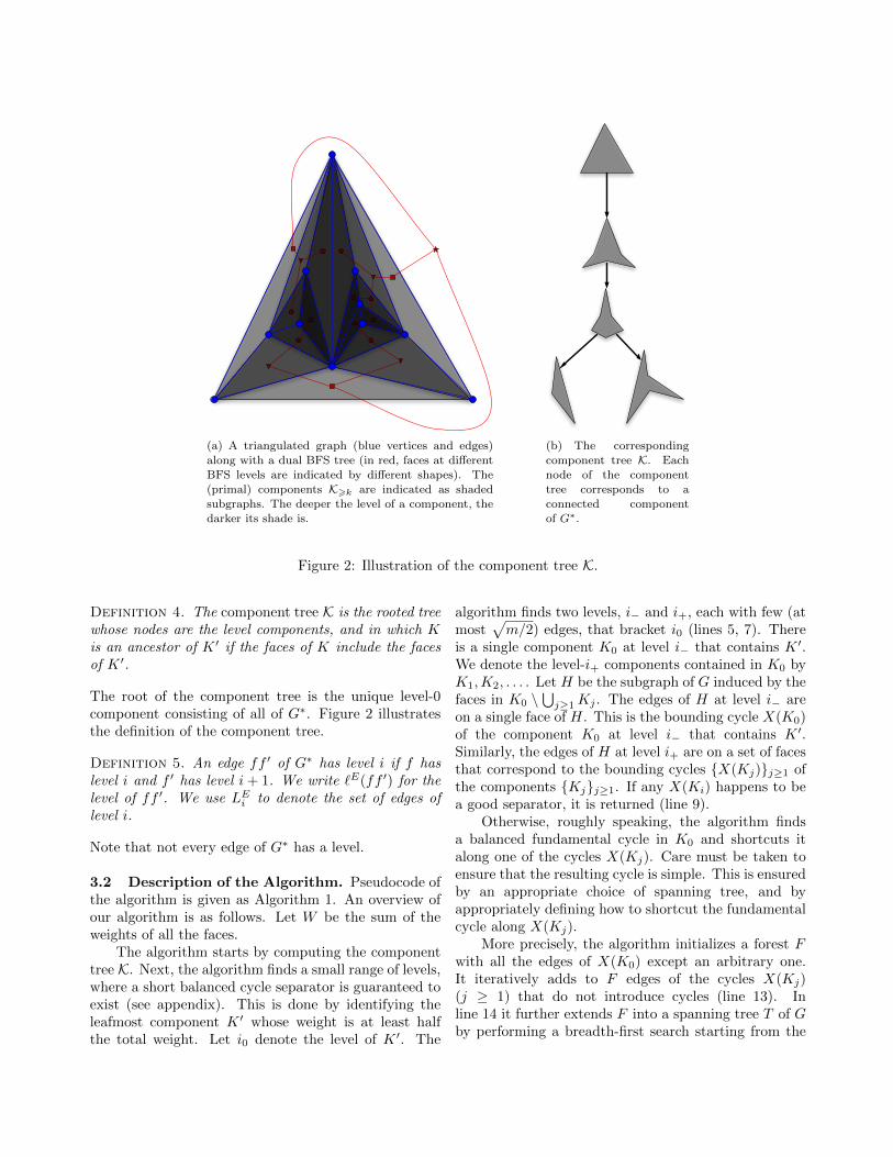
(a) A triangulated graph (blue vertices and edges)along with a dual BFS tree (in red, faces at different

BFS levels are indicated by different shapes). The

(primal) components K>k are indicated as shadedsubgraphs. The deeper the level of a component, the

darker its shade is.

(b) The correspondingcomponent tree K. Each

node of the component

tree corresponds to aconnected component

of G∗.

Figure 2: Illustration of the component tree K.

Definition 4. The component tree K is the rooted treewhose nodes are the level components, and in which Kis an ancestor of K ′ if the faces of K include the facesof K ′.

The root of the component tree is the unique level-0component consisting of all of G∗. Figure 2 illustratesthe definition of the component tree.

Definition 5. An edge ff ′ of G∗ has level i if f haslevel i and f ′ has level i+ 1. We write `E(ff ′) for thelevel of ff ′. We use LE

i to denote the set of edges oflevel i.

Note that not every edge of G∗ has a level.

3.2 Description of the Algorithm. Pseudocode ofthe algorithm is given as Algorithm 1. An overview ofour algorithm is as follows. Let W be the sum of theweights of all the faces.

The algorithm starts by computing the componenttree K. Next, the algorithm finds a small range of levels,where a short balanced cycle separator is guaranteed toexist (see appendix). This is done by identifying theleafmost component K ′ whose weight is at least halfthe total weight. Let i0 denote the level of K ′. The

algorithm finds two levels, i− and i+, each with few (atmost

√m/2) edges, that bracket i0 (lines 5, 7). There

is a single component K0 at level i− that contains K ′.We denote the level-i+ components contained in K0 byK1,K2, . . . . Let H be the subgraph of G induced by thefaces in K0 \

⋃j≥1Kj . The edges of H at level i− are

on a single face of H. This is the bounding cycle X(K0)of the component K0 at level i− that contains K ′.Similarly, the edges of H at level i+ are on a set of facesthat correspond to the bounding cycles {X(Kj)}j≥1 ofthe components {Kj}j≥1. If any X(Ki) happens to bea good separator, it is returned (line 9).

Otherwise, roughly speaking, the algorithm findsa balanced fundamental cycle in K0 and shortcuts italong one of the cycles X(Kj). Care must be taken toensure that the resulting cycle is simple. This is ensuredby an appropriate choice of spanning tree, and byappropriately defining how to shortcut the fundamentalcycle along X(Kj).

More precisely, the algorithm initializes a forest Fwith all the edges of X(K0) except an arbitrary one.It iteratively adds to F edges of the cycles X(Kj)(j ≥ 1) that do not introduce cycles (line 13). Inline 14 it further extends F into a spanning tree T of Gby performing a breadth-first search starting from the

Algorithm 1: Cycle Separator Algorithm

1 triangulate G and choose f∞ arbitrarily2 construct the component tree K3 let K ′ be the maximum-level component with weight at least W/24 let i0 be the level of K ′

5 let i− be the maximum level not exceeding i0 such that |LEi−| ≤

√m/2

6 let K0 be the component at level i− that contains K ′

7 let i+ be the minimum level no less than i0 such that |LEi+| ≤

√m/2

8 let K1,K2, . . . be the components at level i+ contained in K0

9 if W/4 ≤ w(Kj) ≤ 3W/4 for any j ≥ 0 then return X(Kj)10 initialize a forest F with all the edges of X(K0) except for an arbitrary one11 foreach cycle X(Kj) (j ≥ 1) do12 foreach edge e of X(Kj) do13 add e to F if it does not introduce a cycle in F

14 extend F into a spanning tree T of G by a breadth-first search, starting from the component of F thatcontains the edges of X(K0)

15 let T ∗ be the spanning tree of G∗ rooted at f∞ that consists of edges not in T16 let e∗ be a most balanced edge separator of T ∗

17 if e ∈ K0 \⋃

j>0Kj then return the fundamental cycle of e w.r.t. T

18 let j > 0 be such that e ∈ Kj

19 let H be the subgraph of G induced by the faces in K0 \⋃

l>0Kl

20 let H ′ denote the set of faces in T ∗e that belong to H21 let C be the boundary of H ′

22 let C1, C2, . . . , C` be a decomposition of C into simple cycles23 let Hk denote the set of faces enclosed by Ck (for 1 ≤ k ≤ `)24 if w(Hk) ≥W/4 for some 1 ≤ k ≤ ` then return Ck

25 else

26 let r be such that W/4 ≤ w(Kj ∪

⋃1≤k≤rHk

)≤ 3W/4

27 return the boundary of Kj ∪⋃

1≤k≤rHk

component of F that contains the edges of X(K0). Bythis we mean that the BFS is seeded with the componentT of F that contains the edges of X(K0). Whenever avertex in a component T ′ of F is first visited by thesearch, T ′ is added to T , and all the vertices of T ′

are marked as visited. This three-step construction ofthe spanning tree T is important for ensuring that thecycle returned by the procedure is a simple cycle (seeappendix).

The algorithm next computes a spanning tree T ∗

of G∗, consisting of the edges not in T . It finds amost balanced edge separator e∗ in T ∗. If e ∈ H,then the fundamental cycle of e w.r.t. T is returned(line 17). Otherwise, e∗ ∈ Kj for some j ≥ 1 (e∗ /∈ K0

since, by construction, such fundamental cycles are notbalanced). Let T ∗e denote the subtree of T ∗ rooted at e∗.Note that the vertices of T ∗e are exactly the set of facesenclosed by the fundamental cycle of e w.r.t. T . Let H ′

be the set of faces in T ∗e∗ that do not belong to Kj .Let C be the bounding cycle of H ′. C decomposes

into one or more more simple cycles C1, C2, . . . , C`. Ifany Ck is a balanced separator, it is returned (Line 24).Otherwise, there must be a prefix of the Ck’s whoseinterior, together with the faces of component Kj is aset of faces whose boundary is a balanced simple cycleseparator.

We prove in the appendix that Algorithm 1 alwaysreturns a 3/4–balanced simple cycle separator with atmost

√8m edges. As discussed in Section 2, if the

weight is defined as the number of vertices then 3/4can be replaced with 2/3 throughout the paper.

4 Experiments

In this section we evaluate the performance of our al-gorithm and compare it to prior results. One of thestriking findings in the experiments of Holzer et al. [20]is that the Fundamental Cycle Separator algorithm isusually very effective in finding small, balanced cycleseparators. Our goal in this paper is to establish that

our algorithm, which does provide a worst-case guaran-tee on both separator size and balance, is competitivewith FCS both in terms of runtime and in average-casecycle size and balance. We do not directly compare ourresults with the other algorithms presented in [2, 20],primarily because they do not produce simple cycle sep-arators, but also because FCS’s performance was shownto be dominant in most cases.

The FCS algorithm [20] operates as follows: first,it computes a primal BFS tree T spanning the graph.Recall that the edges not in T form a spanning tree T ∗

of the dual graph. Each primal edge e = uv not in Tdefines a fundamental cycle, the one formed by e andthe unique path from u to v in T . Working from leafsof T ∗ towards its root, we can efficiently compute theweight enclosed by each fundamental cycle of T . Thealgorithm returns one of these cycles that is a balancedseparator.

There is a trade-off between balance and cyclelength. If one prefers short cycles, it makes sense toreturn the shortest cycle amongst those that are atleast 2/3–balanced. On the other hand, one cannotnecessarily return the most balanced cycle of lengthO(√m), as FCS has no such cycle size guarantee. In this

case, for both FCS and our algorithm, we return the firstbalanced separator found. Experimenting with differentchoices produced results not significantly different fromthose reported here.

We used two variants of our algorithm and twovariants of FCS in order to illustrate various issues thatarise in our experiments. Recall that our algorithmmay return a level cycle (line 9 in Algorithm 1), afundamental cycle (line 17), or a fundamental-and-level-cycle merger (lines 24, 27). The first variant of ouralgorithm implements the algorithm as presented inSection 3. In particular, it terminates as soon as itencounters a cycle that is a 2/3–balanced separator. Werefer to this variant as unoptimized. The second variant,which we refer to as optimized for balance, computesall candidate separators and returns the most balancedcandidate found.

Similarly, the first variant of FCS is the one thatterminates as soon as it encounters a cycle that is a2/3–balanced separator. We refer to this variant asunoptimized. The second variant, which we refer to asoptimized for length, returns the shortest fundamentalcycle among all those that are 2/3–balanced.

4.1 Data Sets and Experimental Setup. To ef-fectively compare our algorithms, we draw extensivelyfrom the graphs tested experimentally in [2, 20]. Eachgraph is triangulated before testing. Note that thereis some degree of freedom in triangulation (Holzer

et al. [20] use the triangulation routines provided byLEDA). As our graphs are represented by permutationsof the darts (see [25] for more on representing embed-dings), we simply triangulate by walking through thepermutation describing the faces, and if any orbit islarger than three, we insert an edge to produce a trian-gle and reduce the size of the orbit by one.

Below is a list of the classes of graphs.

1. grid are square grid graphs; rect are rectangulargrid graphs. c-grid are two such graphs connectedvia 5 joining vertices that form a perfectly balancedcycle separator.

2. sixgrid graphs are tessellated hexagons.

3. A k-iteration tri graph starts with a triangle, andon each of k iterations, each face except f∞ has anew vertex embedded within it and connected toeach vertex on the face’s boundary.

4. globe graphs approximate spheres, and are imple-mented by wrapping a rect into a cylinder andadding a vertex on top and bottom connected tothe vertices of the top and bottom rows, respec-tively. We call very skewed globes eggs.

5. cylinder graphs are similar to globe graphs, withthe addition of an extra vertex in every square.BFS trees produced for cylinder and (triangu-lated) globe graphs differ substantially.

6. A diameter-k is essentially a narrow, length-kstrip, triangulated in a way that maintains a diam-eter of k and a very small separator (cf. Figure 7in [20]).

7. The airfoil graph is a finite-element mesh of real-world data [9].

8. The graph col is the USA-COL road network usedin the 9th DIMACS Implementation Challenge— Shortest Paths [8], accessible online [7]. Werepeatedly removed vertices of degree at most 1.Then, we interpreted the graph and the coordinatesas a straight-line embedding and we added verticeswhenever two edges intersect geometrically.

All tests are run on a machine with two Intel XeonX5650 processors and 47.3 gigabytes of RAM. The codeis compiled using GCC 4.4.5 targeting x86 64. Theoperating system is Debian. Runtime tests were runsingle-threaded on an otherwise-idle machine. Time ismeasured in CPU clock ticks, using the clock functionin C. Instances were sufficiently large that the clockgranularity is negligible.

0

0.5

1

1.5

2

2.5

3

grid rect globe egg cylinder hex c-grid diameter

CP

U T

icks

(1e

6)

Graph Type

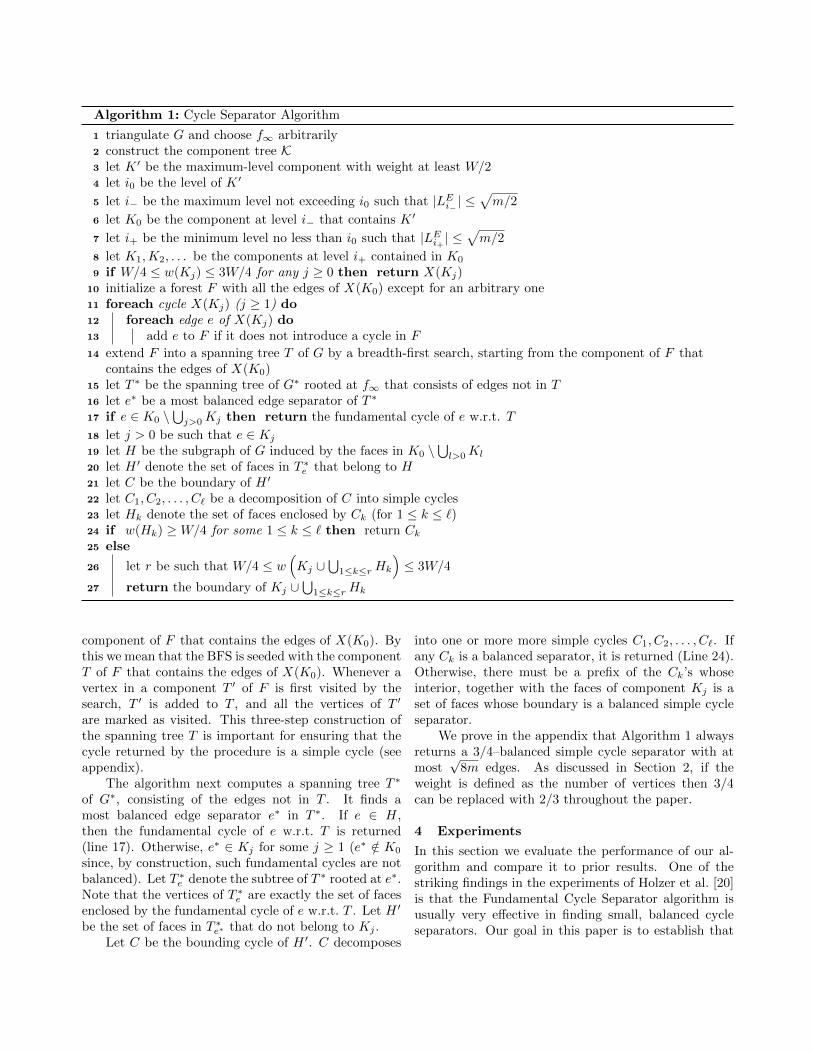
Figure 3: Running time (in CPU clocks) for our algorithm, both optimized for balance (blue) and unoptimized(teal); and for FCS, optimized for length (red) and unoptimized (orange).

4.2 Results and Interpretation. Following Holzeret al. [20], we use whisker plots (Figures 5, 7(a), and7(b)) to show the runtimes for, and the balance andseparator size produced by our algorithm and FCS forvarious types of graphs. For each graph, we tried alarge sample of possible faces as roots of the componenttrees for our algorithm, and possible vertices as rootsof the primal BFS trees for FCS. The box in each plotcorresponds to the middle 50% of values obtained forall choices of root vertices; the whiskers span the entirerange of values observed. The ‘X’ mark in each plotindicates the mean of observed values.

4.2.1 Running Time. Figure 3 shows running timesof the two variants of our algorithm and the two variantsof FCS on various graphs, all with roughly 1,000,000vertices. Specifically, we test on a 1000 by 1000 grid,100 by 10000 rect, 1000 by 1000 globe, 100 by 10000egg, 10000 by 50 cylinder, 700 square hex, 707 by 707c-grid, and a diameter-333333 graph.

It is evident that our algorithm is typically slowerthan FCS, but only by a factor of at most two. This is tobe expected since both our algorithm and FCS computea BFS tree and find a fundamental cycle separator, butour algorithm also performs a dual BFS to compute thecomponent tree and level cycles.

We note that for the egg, cylinder, and diameter

graphs, as well as occasionally, for grid, globe, and

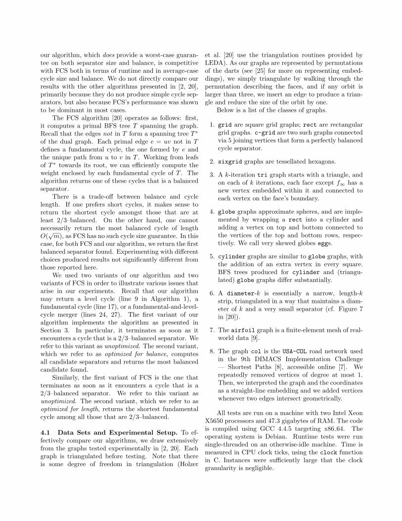
hex, the unoptimized variant of our algorithm is fasterthan both variants of FCS. To explain this behavior,we examined the type of separator returned by theunoptimized variant of our algorithm. These are shownin Figure 4 (left). Recall that the unoptimized variantof our algorithm terminates as soon as it finds a 2/3–balanced cycle. The graphs for which this variant is fastare exactly those for which it typically returns a levelcycle as the separator. For these graphs, this variantonly computes the component tree and level cycles, butdoes not perform a primal BFS nor the search for afundamental cycle separator. In graphs with skewedaspect ratio, such as egg, and cylinder, dual BFS levelsare necessarily small, hence there exists a level cycle thatforms a short, balanced separator.

Interestingly, it is extremely rare that the unopti-mized algorithm resorts to shortcutting a fundmentalcycle separator using cycle levels. This infrequent out-come accounts for a disproportionate amount of the al-gorithm’s complexity (conceptually, but not so much inlines of code), but is required for providing the worst-case guarantee. This implies that complementing theFCS algorithm with computing level cycles (i.e., com-puting a dual BFS) is in itself a useful and efficientsimple cycle separator heuristic.

Figure 4 (right) shows that the balance-optimizedvariant of our algorithm does shortcut fundamentalcycles using level cycles for most starting faces of the

0

20

40

60

80

100

gridrect

eggglobe

hexc-grid

cylinder

diameter

Per

cent

age

Graph Type

0

20

40

60

80

100

gridrect

eggglobe

hexc-grid

cylinder

diameter

Per

cent

age

Graph Type

Figure 4: The type of separator returned by our algorithm – unoptimized (left) and optimized for balance (right)on the graphs used in Figure 3. Teal corresponds to fundamental cycles (line 17 in Algorithm 1), dark blue tolevel cycles (line 9), and purple to a fundamental-and-level cycle merger (lines 24–27).

egg graph and for some of the globe graphs. In thoseinstances, the time spent on shortcutting the FCS is alittle less than the time spent on finding the FCS.

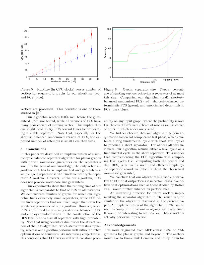
Figure 5 shows the running time as a function ofthe size of various square grids. As expected, bothFCS and our algorithm appear to scale linearly in thenumber of vertices. The change in minimum runningtime around 20 million vertices can be most likelyattributed to caching effects. Again, we see here that,on average, our algorithm takes no more than twiceas long as FCS. The slopes of the lines of best-fit(3.1 and 1.9 for our algorithm and FCS, respectively)suggest that our algorithm tends to be 1.6 times slowerthan FCS. As shown in Figure 7(b), one might haveto run FCS several times to locate a separator withsize and balance within the guarantees provided by ouralgorithm. Therefore, we consider the runtime of ouralgorithm to be competitive.

4.2.2 Separator Balance and Size. Figures 7(a)and 7(b) show results for balance and size, respectively.Each graph tested (except for colorado) has approxi-mately 10,000 vertices and is triangulated. In particu-lar, grid is 100 by 100, rect is 10 by 1000, egg is a10 by 1000 globe, globe is 100 by 100, hex is 70 by 70,c-grid is 71 by 71, tri is ten iterations, cylinder is1000 by 5, and diameter has diameter 3333.

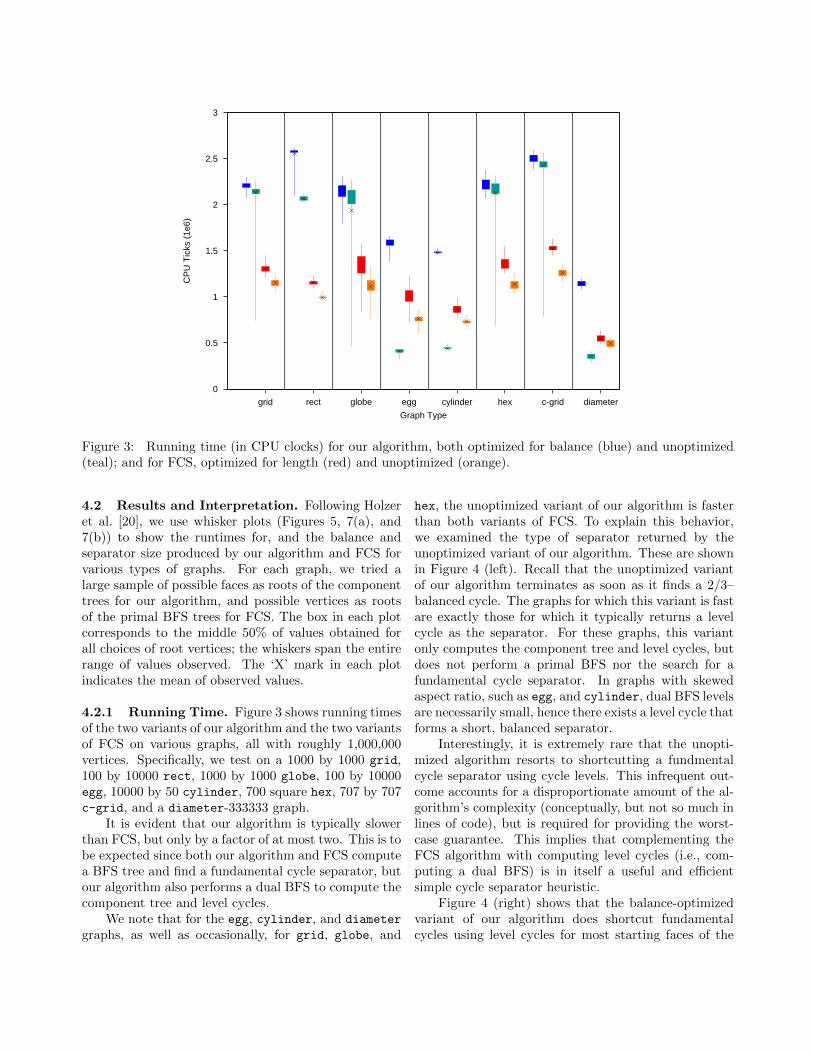
In Figure 7(a), we see that unoptimized FCS neverproduces significantly more balanced separators thanour unoptimized algorithm. However, for the graphsegg, cylinder, tri, and diameter, our algorithm pro-duces nearly perfectly balanced separators every time,

whereas FCS tends to find separators that are 2/3–balanced. Recall from Figure 4 and the discussion abovethat, for these graphs, our algorithm typically returnsa level cycle as the separator. Since candidate level cy-cles are searched for starting from the median–balancedlevel (level i0 in Section 3), and since in these graphs,BFS levels consist of few edges, the algorithm finds smalllevel cycles that are nearly perfectly balanced. We haveverified that optimizing both algorithms for balance (i.e.taking the most balanced separator encountered) elimi-nates those differences. Note, however, that optimizingFCS for balance is not guaranteed to return a short sep-arator. In fact, for cylinder graphs, this is often thecase.

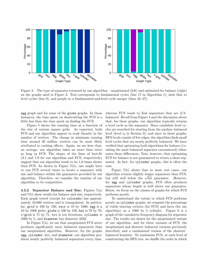
Figure 7(b) shows that in most test cases, ouralgorithm returns slightly longer separators than FCS,but still well below the

√8m guarantee. However,

for egg and cylinder graphs, FCS often producesseparators whose length is well above our guarantee.Below, we focus on the classes of graphs for which FCSperforms poorly.

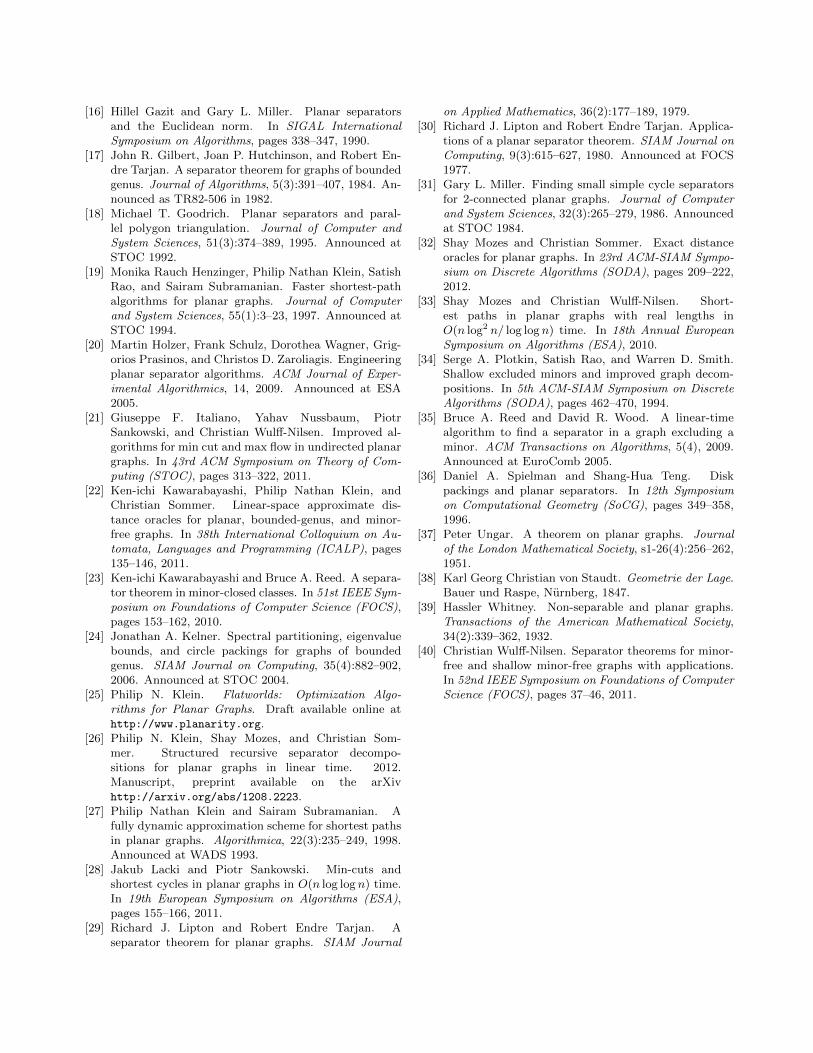
To understand the extent to which FCS performspoorly on cylinder graphs, we compute the percentageof viable starting vertices (for FCS) and faces (for ouralgorithm) on a 1000 by 5 cylinder. Figure 6 is agraph of the cumulative frequency diagram for separatorsize. The results are shown for the unoptimized variantof our algorithm, and for three variants of FCS: theunoptimized and shortest–balanced versions previouslydescribed, and a randomized version of the shortest–balanced heuristic. To randomize FCS, at each level ofconstructing the BFS tree, we shuffle the order in which

0

20

40

60

80

100

120

140

0 5 10 15 20 25 30 35 40 45

CP

U T

icks

(1e

6)

Number of Vertices (1e6)

Figure 5: Runtime (in CPU clocks) versus number ofvertices for square grid graphs for our algorithm (red)and FCS (blue).

vertices are processed. This heuristic is one of thosestudied in [20].

Our algorithm reaches 100% well before the guar-anteed

√8m size bound, while all versions of FCS have

many poor choices of starting vertex. This implies thatone might need to try FCS several times before locat-ing a viable separator. Note that, especially for theshortest–balanced randomized version of FCS, the ex-pected number of attempts is small (less than two).

5 Conclusions

In this paper we described an implementation of a sim-ple cycle balanced separator algorithm for planar graphswith proven worst-case guarantees on the separator’ssize. To the best of our knowledge, the only other al-gorithm that has been implemented and guarantees asimple cycle separator is the Fundamental Cycle Sepa-rator Algorithm. However, unlike our algorithm, FCSdoes not provide worst-case size guarantees.

Our experiments show that the running time of ouralgorithm is comparable to that of FCS on all instances.We demonstrate families of graphs for which our algo-rithm finds extremely small separators, while FCS of-ten finds separators that are much larger than even theworst-case guarantee of our algorithm. However, whenFCS is optimized for returning a shortest balanced FCS,and employs randomization in the construction of theBFS tree, it finds a small separator with high probabil-ity. Note that using heuristics diminishes the attractive-ness of the FCS algorithm, which stems from its simplic-ity, whereas our algorithm performs well without furtheroptimizations or heuristics. An interesting conjecture inthis context is that FCS works well with constant prob-

0

20

40

60

80

100

sqrt(8m) 1 10 100 1000

Per

cent

age

Separator size

Figure 6: X-axis: separator size. Y-axis: percent-age of starting vertices achieving a separator of at mostthis size. Comparing our algorithm (teal), shortest–balanced randomized FCS (red), shortest–balanced de-terministic FCS (green), and unoptimized deterministicFCS (dark blue).

ability on any input graph, where the probability is overthe choices of BFS trees (choice of root as well as choiceof order in which nodes are visited).

We further observe that our algorithm seldom re-quires the somewhat complicated last phase, which com-bines a long fundamental cycle with short level cyclesto produce a short separator. For almost all test in-stances, our algorithm returns either a level cycle or afundamental cycle as the short separator. This impliesthat complementing the FCS algorithm with comput-ing level cycles (i.e., computing both the primal anddual BFS) is in itself a useful and efficient simple cy-cle separator algorithm (albeit without the theoreticalworst-case guarantee).

We conclude that our algorithm is a viable alterna-tive to FCS that outperforms it in certain cases. We be-lieve that optimizations such as those studied by Holzeret al. would further enhance its performance.

An interesting direction for future work is imple-menting the separator algorithm in [26], which is quitesimilar to the algorithm discussed in the current pa-per. An implementation of the algorithm in [26] can beused to compute r–divisions in asymptotic linear time.It would be interesting to see how well that algorithmactually performs in practice.

Acknowledgements

This work originated from MIT course 6.889 on “Al-gorithms for planar graphs and beyond.” The authorswould like to thank Erik Demaine and Philip Klein for

1/3

0.35

0.4

0.45

0.5

grid

rect

globe

egg

cylinder

hex

c-grid

diameter

tri colorado

Sep

arat

or B

alan

ce

Graph Type

(a) Separator balance (number of vertices in smaller part

divided by the total number of vertices) for our unoptimizedalgorithm (red) with unoptimized FCS (green).

sqrt(8)

0

2

4

6

8

10

12

grid

rect

globe

egg

cylinder

hex

c-grid

diameter

tri colorado

Sep

arat

or S

ize

Graph Type

(b) Separator size divided by√m for our unoptimized algo-

rithm (red), unoptimized FCS (green), and shortest–balancedFCS (blue).

Figure 7: Separator balance and size for various graphs

fruitful discussions. Additionally, we thank Philip Kleinand his team for providing us with their planar graphlibrary.

CS was partially supported by the Swiss NationalScience Foundation. Work was conducted while CS wasat MIT. SM was partially supported by National ScienceFoundation Grants CCF-0964037 and CCF-1111109.

References

[1] Lyudmil Aleksandrov and Hristo Nicolov Djidjev. Lin-ear algorithms for partitioning embedded graphs ofbounded genus. SIAM Journal on Discrete Mathemat-ics, 9(1):129–150, 1996.

[2] Lyudmil Aleksandrov, Hristo Nicolov Djidjev, HuaGuo, and Anil Maheshwari. Partitioning planar graphswith costs and weights. ACM Journal of ExperimentalAlgorithmics, 11, 2006. Announced at ALENEX 2002.

[3] Noga Alon, Paul D. Seymour, and Robin Thomas. Aseparator theorem for nonplanar graphs. Journal of theAmerican Mathematical Society, 3(4):801–808, 1990.Announced at STOC 1990.

[4] Punyashloka Biswal, James R. Lee, and Satish Rao.Eigenvalue bounds, spectral partitioning, and metricaldeformations via flows. Journal of the ACM, 57(3),2010. Announced at FOCS 2008.

[5] Glencora Borradaile, Philip N. Klein, Shay Mozes, Ya-hav Nussbaum, and Christian Wulff-Nilsen. Multiple-source multiple-sink maximum flow in directed planargraphs in near-linear time. In 52nd IEEE Symposiumon Foundations of Computer Science (FOCS), pages170–179, 2011.

[6] Sergio Cabello. Many distances in planar graphs.

Algorithmica, 62(1–2):361–381, 2012. Announced atSODA 2006.

[7] Camil Demetrescu, Andrew Goldberg, and DavidJohnson. 9th DIMACS Implementation Challenge— Shortest Paths. http://www.dis.uniroma1.it/

challenge9/download.shtml; accessed 21 Oct 2012.[8] Camil Demetrescu, Andrew V. Goldberg, and David S.

Johnson. Implementation challenge for shortest paths.In Encyclopedia of Algorithms. 2008.

[9] Ralf Diekmann and Robert Preis, 1998.http://www2.cs.uni-paderborn.de/fachbereich/AG/

monien/RESEARCH/PART/GRAPHS/FEM2.tar; accessed21 Oct 2012.

[10] Hristo Nicolov Djidjev. On the problem of partition-ing planar graphs. SIAM Journal on Algebraic andDiscrete Methods, 3:229–240, 1982.

[11] Hristo Nicolov Djidjev. A linear algorithm for par-titioning graphs of fixed genus. Serdica. Bulgariacaemathematicae publicationes, 11(4):369–387, 1985. An-nounced in Comptes Rendus de l’Academie Bulgare desSciences, 34:643–645, 1981.

[12] Hristo Nicolov Djidjev and Shankar M. Venkatesan.Reduced constants for simple cycle graph separation.Acta Informatica, 34:231–243, 1997.

[13] Jittat Fakcharoenphol and Satish Rao. Planar graphs,negative weight edges, shortest paths, and near lineartime. Journal of Computer and System Sciences,72(5):868–889, 2006. Announced at FOCS 2001.

[14] Lamis M. Farrag. Applications of graph partitioningalgorithms to terrain visibility and shortest path prob-lems. Master’s thesis, School of Computer Science,Carleton University, 1998.

[15] Greg N. Frederickson. Fast algorithms for shortestpaths in planar graphs, with applications. SIAMJournal on Computing, 16(6):1004–1022, 1987.

[16] Hillel Gazit and Gary L. Miller. Planar separatorsand the Euclidean norm. In SIGAL InternationalSymposium on Algorithms, pages 338–347, 1990.

[17] John R. Gilbert, Joan P. Hutchinson, and Robert En-dre Tarjan. A separator theorem for graphs of boundedgenus. Journal of Algorithms, 5(3):391–407, 1984. An-nounced as TR82-506 in 1982.

[18] Michael T. Goodrich. Planar separators and paral-lel polygon triangulation. Journal of Computer andSystem Sciences, 51(3):374–389, 1995. Announced atSTOC 1992.

[19] Monika Rauch Henzinger, Philip Nathan Klein, SatishRao, and Sairam Subramanian. Faster shortest-pathalgorithms for planar graphs. Journal of Computerand System Sciences, 55(1):3–23, 1997. Announced atSTOC 1994.

[20] Martin Holzer, Frank Schulz, Dorothea Wagner, Grig-orios Prasinos, and Christos D. Zaroliagis. Engineeringplanar separator algorithms. ACM Journal of Exper-imental Algorithmics, 14, 2009. Announced at ESA2005.

[21] Giuseppe F. Italiano, Yahav Nussbaum, PiotrSankowski, and Christian Wulff-Nilsen. Improved al-gorithms for min cut and max flow in undirected planargraphs. In 43rd ACM Symposium on Theory of Com-puting (STOC), pages 313–322, 2011.

[22] Ken-ichi Kawarabayashi, Philip Nathan Klein, andChristian Sommer. Linear-space approximate dis-tance oracles for planar, bounded-genus, and minor-free graphs. In 38th International Colloquium on Au-tomata, Languages and Programming (ICALP), pages135–146, 2011.

[23] Ken-ichi Kawarabayashi and Bruce A. Reed. A separa-tor theorem in minor-closed classes. In 51st IEEE Sym-posium on Foundations of Computer Science (FOCS),pages 153–162, 2010.

[24] Jonathan A. Kelner. Spectral partitioning, eigenvaluebounds, and circle packings for graphs of boundedgenus. SIAM Journal on Computing, 35(4):882–902,2006. Announced at STOC 2004.

[25] Philip N. Klein. Flatworlds: Optimization Algo-rithms for Planar Graphs. Draft available online athttp://www.planarity.org.

[26] Philip N. Klein, Shay Mozes, and Christian Som-mer. Structured recursive separator decompo-sitions for planar graphs in linear time. 2012.Manuscript, preprint available on the arXivhttp://arxiv.org/abs/1208.2223.

[27] Philip Nathan Klein and Sairam Subramanian. Afully dynamic approximation scheme for shortest pathsin planar graphs. Algorithmica, 22(3):235–249, 1998.Announced at WADS 1993.

[28] Jakub Lacki and Piotr Sankowski. Min-cuts andshortest cycles in planar graphs in O(n log logn) time.In 19th European Symposium on Algorithms (ESA),pages 155–166, 2011.

[29] Richard J. Lipton and Robert Endre Tarjan. Aseparator theorem for planar graphs. SIAM Journal

on Applied Mathematics, 36(2):177–189, 1979.[30] Richard J. Lipton and Robert Endre Tarjan. Applica-

tions of a planar separator theorem. SIAM Journal onComputing, 9(3):615–627, 1980. Announced at FOCS1977.

[31] Gary L. Miller. Finding small simple cycle separatorsfor 2-connected planar graphs. Journal of Computerand System Sciences, 32(3):265–279, 1986. Announcedat STOC 1984.

[32] Shay Mozes and Christian Sommer. Exact distanceoracles for planar graphs. In 23rd ACM-SIAM Sympo-sium on Discrete Algorithms (SODA), pages 209–222,2012.

[33] Shay Mozes and Christian Wulff-Nilsen. Short-est paths in planar graphs with real lengths inO(n log2 n/ log log n) time. In 18th Annual EuropeanSymposium on Algorithms (ESA), 2010.

[34] Serge A. Plotkin, Satish Rao, and Warren D. Smith.Shallow excluded minors and improved graph decom-positions. In 5th ACM-SIAM Symposium on DiscreteAlgorithms (SODA), pages 462–470, 1994.

[35] Bruce A. Reed and David R. Wood. A linear-timealgorithm to find a separator in a graph excluding aminor. ACM Transactions on Algorithms, 5(4), 2009.Announced at EuroComb 2005.

[36] Daniel A. Spielman and Shang-Hua Teng. Diskpackings and planar separators. In 12th Symposiumon Computational Geometry (SoCG), pages 349–358,1996.

[37] Peter Ungar. A theorem on planar graphs. Journalof the London Mathematical Society, s1-26(4):256–262,1951.

[38] Karl Georg Christian von Staudt. Geometrie der Lage.Bauer und Raspe, Nurnberg, 1847.

[39] Hassler Whitney. Non-separable and planar graphs.Transactions of the American Mathematical Society,34(2):339–362, 1932.

[40] Christian Wulff-Nilsen. Separator theorems for minor-free and shallow minor-free graphs with applications.In 52nd IEEE Symposium on Foundations of ComputerScience (FOCS), pages 37–46, 2011.

A Correctness of Algorithm 1

A.1 Simple Cycle

Lemma A.1. For every Ki (i ≥ 0) there is a single edgee∗ ∈ T ∗ whose rootward endpoint is not a face of Ki andwhose other endpoint is a face of Ki.

Proof. The claim is true for i = 0 since the root of T ∗

is f∞ and since exactly one edge of X(K0) is in T ∗. Fori ≥ 1, assume there is more than one edge where T ∗

enters Ki. Consider two such edges e∗1, e∗2. Consider the

embedding of H inherited from G. The unique path inT ∗ between e∗1 and e∗2 partitions the embedding of Hinto at least two regions such that the vertices of X(Ki)are not all in a single region. Since T ∗ does not containany edges of the forest F , this contradicts the fact thatthe vertices of X(Ki) are connected in F . �

For a given i ≥ 0, we say that T ∗ enters Ki at theunique edge e of X(Ki) that belongs to T ∗. We usethe edge e at which T ∗ enters Ki to define an order onthe vertices of X(Ki). Namely, the order in which thevertices of X(Ki) are encountered in a clockwise walkalong X(Ki), starting from e.

Lemma A.2. Fix j ≥ 1. Let x1, x2, . . . x` be the setof vertices in X(K0) ∩X(Kj), in clockwise order alongX(K0), starting from the edge of X(K0) at which T ∗

enters K0. Then this is also the order in which thesevertices are visited in clockwise order along X(Kj),starting from the edge of T ∗ at which T ∗ enters Kj.

Proof. The lemma is trivial for ` < 2. Assume,therefore, that ` ≥ 2. T ∗ enters K0 between x` and x1.Lemma A.1 implies that T ∗ enters Kj between x` andx1 as well. Suppose that xi+1 does not follow xi inthe clockwise order of vertices along X(Kj). Theneither X(K0) does not enclose X(Kj), or X(K0) is nota simple cycle – a contradiction.

We establish some properties of T and T ∗ that arecritical for our implementation. The first two lemmasfollow immediately from the definition of T .

Lemma A.3. Let u, v be vertices on X(K0). Theunique u-to-v path in T consists only of edges of X(K0).�

Lemma A.4. Let u, v be vertices on X(Kj) for any fixedj ≥ 0. The unique u-to-v path in T consists only ofedges in F . �

Lemma A.5. Let u, v be vertices on X(Ki) for any fixedi ≥ 1. Any u-to-v path P that consists only of edgesof ∪j≥1X(Kj) uses only edges of X(Ki).

Proof. The proof is by contradiction. Assume P con-tains some edge that does not belong to X(Ki). With-out loss of generality, P contains no edges of X(Ki)(otherwise choose such a subpath of P ). Let C be asimple cycle formed by a u-to-v subpath of X(Ki) andby P . Observe that C consists of level i+ edges, soall faces enclosed by C have level at least i+. How-ever, since the X(Kj)’s are edge disjoint, C must en-close some face that is not enclosed by any X(Kj), i.e.,a face whose level is smaller than i+, a contradiction. �

eu

v

T*

X(K0)X(Kj)

C2

C1

u-

u+

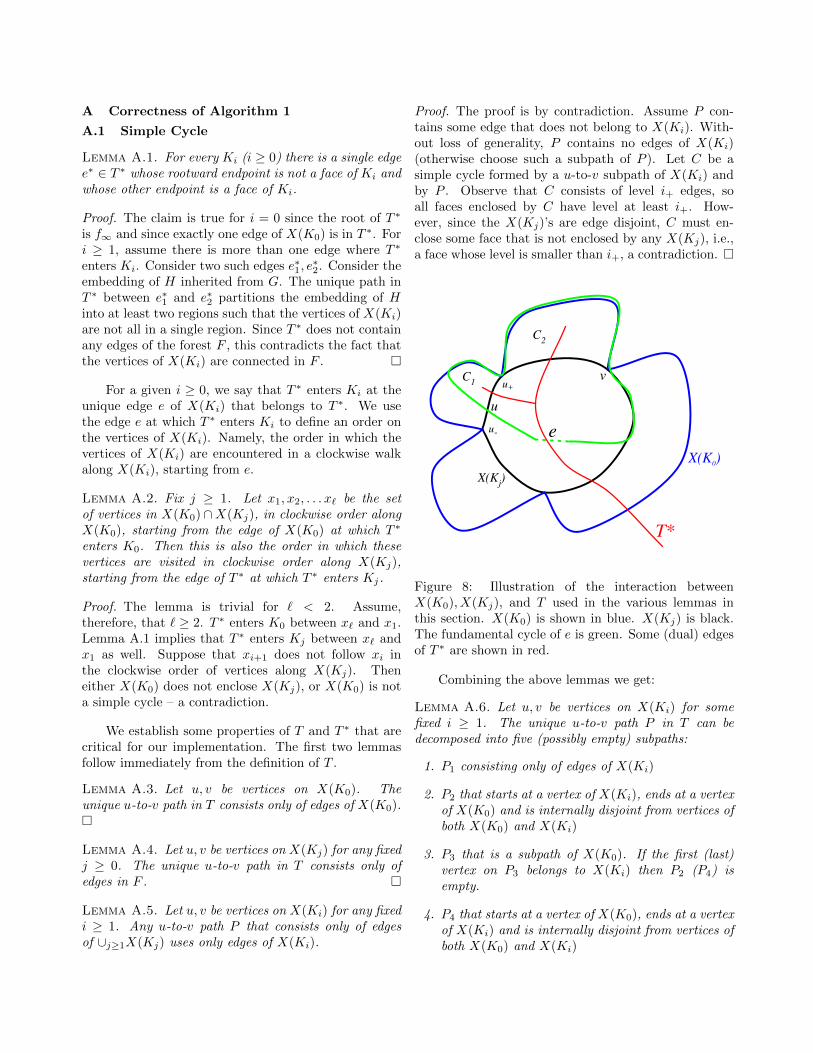
Figure 8: Illustration of the interaction betweenX(K0), X(Kj), and T used in the various lemmas inthis section. X(K0) is shown in blue. X(Kj) is black.The fundamental cycle of e is green. Some (dual) edgesof T ∗ are shown in red.

Combining the above lemmas we get:

Lemma A.6. Let u, v be vertices on X(Ki) for somefixed i ≥ 1. The unique u-to-v path P in T can bedecomposed into five (possibly empty) subpaths:

1. P1 consisting only of edges of X(Ki)

2. P2 that starts at a vertex of X(Ki), ends at a vertexof X(K0) and is internally disjoint from vertices ofboth X(K0) and X(Ki)

3. P3 that is a subpath of X(K0). If the first (last)vertex on P3 belongs to X(Ki) then P2 (P4) isempty.

4. P4 that starts at a vertex of X(K0), ends at a vertexof X(Ki) and is internally disjoint from vertices ofboth X(K0) and X(Ki)

5. P5 consisting only of edges of X(Ki)

Proof. Refer to Figure 8. Let P1, P5 be the maximalprefix and suffix of P consisting only of edges of X(Ki).Let P ′ denote the subpath of P between P1 and P5. If P ′

is non-empty, then it is a path between vertices ofX(Ki)that includes some edge not in X(Ki). By Lemma A.5,it cannot consist solely of edges in ∪j≥1X(Kj). ByLemma A.4, P consists only of edges of F . Hence, P ′

must include some edge of X(K0). By Lemma A.3, allvertices of X(K0) in P form a subpath of P that consistsonly of edges of X(K0). Hence this is also a subpathof P ′. Denote it by P3. The remaining two subpathsof P ′, which we denote by P2 and P4, consist only ofedges not in X(K0). By Lemma A.4, P2 and P4 donot contain any vertices of X(Ki), other than the firstvertex of P2 and the last vertex of P4. Hence, if the first(last) vertex of P3 belongs to X(Ki), P2 (P4) must beempty. �

Consider the case where e∗ ∈ Kj . Let C be thefundamental (and thus simple) cycle of T w.r.t. e. Let Qbe the maximal subpath of C that contains e and has nointernal vertices that are vertices of X(Kj). Write C =P ◦Q. Since P is a path in T between vertices that areon X(Kj), it can be written as P = P1◦P2◦P3◦P4◦P5,as specified in Lemma A.6. Let u, v be the endpointsof P2 and P4, respectively, that belong to X(Kj), whereu appears before v in the order of vertices of X(Kj).

Lemma A.7. The unique path P ′ = P2 ◦ P3 ◦ P4 in Tbetween u and v visits no vertices of X(Kj) that appearbefore u or after v in the order of vertices along X(Kj).

Proof. By Lemma A.6, since P2 and P4 are internallyvertex disjoint from X(Kj), it suffices to show that P3

visits no vertices of X(Kj) that appear before u orafter v in the order of vertices along X(Kj). If P3

contains no vertices of X(Kj), the lemma is triviallytrue. Otherwise, X(K0) ∩X(Kj) is non empty.

Let u− (u+) be the vertex in X(K0) ∩X(Kj) thatweakly precedes (follows) u in the order of verticesalong X(Kj). Assume first, that such predecessor andsuccessor exist. Similarly, Let v− (v+) be the vertex inX(K0) ∩ X(Kj) that precedes (follows) v in the orderof vertices along X(Kj). Let Q0

u be the unique u−-to-u+ subpath of X(K0) that does not include the edgeat which T ∗ enters X(K0). Let Qj

u be the uniqueu−-to-u+ subpath of X(Kj) that does not include theedge at which T ∗ enters X(Kj). By planarity, P2 isconfined to the interior of the cycle formed by Q0

u andQj

u. Hence, the first vertex x of P3 must either be u (incase u ∈ X(K0), or an internal vertex of Q0

u. A similarargument shows that the last vertex y of P3 is either

v or an internal vertex of Q0v (where Q0

v is the uniquev−-to-v+ subpath of X(K0) that does not include theedge at which T ∗ enters X(K0)).

Since neither P2 nor P4 use edges of T ∗, and sinceP ′ is simple, x must precede y in the order of verticesof X(K0) (see Figure 8). Recall that P3 is the uniquex-to-y subpath of X(K0) that does not include the edgeat which T ∗ enters X(K0). Therefore the vertices inP3 appear in increasing order of the vertices of X(K0).This means that if P3 contains a vertex of X(Kj), thefirst such vertex is u+, and the last such vertex is v−.It follows, by Lemma A.2 that P3 only visits verticesof X(Kj) that follow u and precede v in the order ofvertices along X(Kj).

The case where the predecessor u− or the succes-sor u+ does not exist is handled in a similar manner.Note that only one of these can happen simultaneously,since we assume K(X0) ∩ X(Kj) 6= ∅. Also note thatthis implies u /∈ X(K0) since otherwise u = u− = u+.Suppose the predecessor does not exist (the other caseis symmetric). In this case we define u− to be the firstvertex of X(K0). As above, let Q0

u be the unique u−-to-u+ subpath of X(K0) that does not include the edgeat which T ∗ enters X(K0). Note that u+ is the onlyvertex of Q0

u that belongs to X(Kj). Since P2 does notuse any edges of T ∗, the first vertex x of P3 must be avertex of Q0

u. The remainder of the argument proceedsas above. �

Let H be the subgraph of G induced by the facesin K0 \ ∪i>0Ki. Let H ′ denote the set of faces in T ∗ethat belong to H. The boundary C of H ′ consists of thepath P ′ described in Lemma A.7, and of the subpathQ of X(Kj) between u and v that does not containthe edge of T ∗ that enters Kj . Lemma A.7 showsthat even though C might not be a simple cycle, thenon-simplicities arise in a structured, monotonic way.Specifically, the vertices of P ′ that belong to X(Kj) areall vertices ofQ and appear in the same order along bothP ′ and Q. Put in other words, and using the notation{Ci}, {Hi} as defined in the algorithm (lines 21–23), wehave the following lemma.

Lemma A.8. The cycle returned by the algorithm issimple.

Proof. The cycle returned in Lines 9 is simple sincecomponent boundaries are simple cycles. The cyclereturned in Line 17 is simple since it is a fundamentalcycle. The cycle returned in Line 24 is simple bydefinition of the Ck’s. It remains to show that theboundary of Kj∪

⋃kHk is a simple cycle. The boundary

of Kj ∪⋃

kHk consists of a prefix of P ′ and of Q, thepath consisting of a suffix ofQ and of the edges ofX(Kj)

that do not belong to Q The lemma follows since, by theargument preceding this lemma, P ′ and Q are vertexdisjoint, and since both are simple paths with the sameendpoints. �

We have shown that the cycle returned by thealgorithm is simple. We next argue that this simplecycle is a short balanced separator.

A.2 Balance and Cycle Length

Lemma A.9. The simple cycle returned by the algo-rithm is 3/4–balanced

Proof. Clearly, the cycles returned in Lines 9, 17, or 24are balanced separators. It only remains to argue thatif Line 26 is reached, then there exists an r such thatKj ∪

⋃1≤k≤rHk is 3/4–balanced. By construction of T ,

the fundamental cycle of e w.r.t. T is enclosed byX(K0). Since this fundamental cycle is a balancedseparator (albeit not a short one), this implies that

w(Kj ∪

⋃1≤k≤`Hk

)≥ W/4. Since the conditions in

line 9 and 24 are both false, w(Kj) < W/4 and theweight enclosed by any individual Ck is at most W/4.Hence, an appropriate r must exist. �

Lemma A.10. The forest F consists of at most√

2medges.

Proof. By choice of the levels i− and i+, each levelconsists of at most

√m/2 edges. Since F consists of

at most all edges of these two levels, it consists of atmost

√2m edges. �

Lemma A.11. Let u be a vertex in H. The root-to-upath in T consists of at most

√m/2 edges that do not

belong to F .

Proof. Let f be a face to which u is incident. The levelof f is between i− and i+. By definition of levels offaces, there exists a face f ′ that is incident to X(K0)and whose distance in the dual of H from f is at most(i+− i−). Since each face is a triangle, this implies thatthere exists a path in H from u to some vertex of X(K0)whose length is at most (i+−i−)/2. Since T is obtainedfrom F by breadth-first search, the root-to-u path in Tconsists of at most (i+ − i−)/2 edges not in F .

It remains to bound i+ − i−. Since the cyclesbounding different components are edge disjoint, andsince every level between i− and i+ consists of at least√m/2 edges, (i+− i−)∗ (

√m/2) < m. This shows that

i+− i− <√

2m. Hence, the root-to-u path in T consistsof at most

√m/2 edges that are not in F . �

Theorem A.1. The algorithm returns a 3/4–balancedsimple cycle separator with at most

√8m edges.

Proof. Lemma A.8 shows that the cycle returned bythe algorithm is simple. Lemma A.9 shows that it isa 3/4–balanced separator. It remains to bound thelength of the cycle. The cycle returned in Line 9consist of at most

√m/2 edges. The fundamental cycle

returned in Line 17 consists of two paths of T betweenthe endpoints of e and vertices on X(K0) and from asubpath of X(K0). The length of each of the former twopaths is bounded by Lemma A.11 by

√m/2. By choice

of i−, the length of X(K0) is at most√m/2. Hence,

the length of the cycle returned in Line 17 is at most3√m/2 <

√8m.

The cycle returned in Line 27 consists of edgesof X(Kj), edges of X(K0) and two paths in T betweenvertices of X(Kj) and vertices of X(K0). By choiceof i− and i+, the length of X(K0) and the lengthof X(Kj) are both bounded by

√m/2. Note that

the edges of X(K0) and X(Kj) belong to F . ByLemma A.11, each of the paths of T consists of atmost

√m/2 edges not in F . Hence the boundary

of Kj ∪⋃

1≤k≤rHk consists of at most 4√m/2 =

√8m

edges. �