short-circuit contributions from fully-rated …714792/fulltext01.pdfdegree project in short-circuit...

Degree project in

Short-circuit Contributions fromFully-rated Converter Wind Turbines

Modeling and simulation of steady-state short-circuit contributions from FRC wind turbines

in offshore wind power plants

JOAKIM AHNLUND

Stockholm, Sweden 2014

XR-EE-EPS 2014:004

Electric Power SystemsSecond Level,

Short-circuit contributions from fully-ratedconverter wind turbines

Modeling and simulation of steady-state short-circuit contributions from FRC windturbines in offshore wind power plants

JOAKIM AHNLUND

Master’s Thesis at EESSupervisor: Amin Nasri

Examiner: Mehrdad Ghandhari

April 2014

iii

Abstract

In recent years there has been an increase in wind power plants installed outat sea. The generated power of wind turbine generators (WTGs) are collectedthrough numerous subsea cables into a single hub, the offshore platform. Sub-sequently, this platform is interconnected with the onshore main grid througha further stretch of cable. In the event of a fault, a sudden increase in cur-rent, so called short-circuit current, will occur somewhere in the system. Theshort-circuit current will, depending on the duration and location of the fault,potentially harm the power system. In order to accurately determine the di-mensions and rating of the equipment installed in the offshore wind power plant(OWPP), the magnitude of this current needs to be studied. Furthermore,depending on the country in which the OWPP is installed, the transmissionsystem operator (TSO) might pose different low-voltage-ride-through (LVRT)requirements on the system. One such requirement is that the installed tur-bines should provide voltage regulation through injection of reactive current.A type of generator able to achieve this is a so-called fully-rated converter windturbine generator (FRC WTG). Through a power electronic interface, the re-active and active current components of the generator can be freely controlled.With a high level of reactive current injected during a fault in the OWPP,the short-circuit contribution from these FRC WTGs needs to be evaluated.In this master’s thesis, a method has been developed in order to determinethe steady-state short-circuit contribution from multiple FRC WTGs. Thismethodology is based on an iterative algorithm, and has been implemented inthe simulation tool PowerFactory. To evaluate the performance of the method,two case studies were performed. In order to improve simulation times, analready existing WTG aggregation model has been implemented to reduce thenumber of turbines in the test system. From the results, it is concluded that themethod obtains the expected FRC WTG short-circuit currents with sufficientaccuracy. Furthermore, the deviation from the expected results are evaluatedusing a numerical tool. This project was initiated and conducted at ABB inVästerås, Sweden.

iv

Sammanfattning

Under de senaste åren har det skett en ökning av vindkraftparker installeradetill havs. Den genererade effekten från varje enskild vindturbin samlas upp viahavskablar till en platform där den transformeras till en högre spänningsni-vå. Från platformen transporteras effekten sedan vidare in mot land genom enlängre kabel som ansluts till en landstation. Landstationen i sin tur är anslutentill stamnätet. I händelsen av ett fel någonstans i system kommer höga ström-mar att rusa, så kallade kortslutningsströmmar. Beroende på varaktigheten ochplatsen för felet kan dessa strömmar vara skadliga för systemet. För att på ettnoggrannt sätt bestämma dimensioner och märkvärden på den utrustning somska installeras i systemet måste därför storleken på denna ström studeras. Ut-över detta så kan nätoperatören, beroende på vilket land som vindkraftparkenär installerad i, ställa olika krav på hur systemet ska hantera spänningsfall ifelsituationer. Ett sådant krav är att vindturbinerna i parken måste bistå medspänningsreglering medelst injektion av reaktiv ström. En typ av vindturbinsom klarar av att uppfylla dessa krav är så kallade helomriktade vindturbi-ner. Via en effektelektronisk frikoppling kan generatorns aktiva samt reaktivaströmbidrag kontrolleras fritt. Då en stor mängd reaktiv ström eventuellt kaninjiceras på grund utav en kortslutning i parken måste bidraget från dessa tur-biner utvärderas. Under detta examensarbete har en metod för att bestämmadet stationära kortslutningsbidraget från ett flertal helomriktade turbiner ut-vecklats. Metoden är baserad på en iterativ algoritm och har implementeratsi simuleringsverktyget PowerFactory. För att utvärdera metodens prestandahar två fallstudier utförts. I avsikt att förbättra simuleringstiden har en re-dan befintlig metod för aggregering använts för att minska antalet turbiner itestkretsen. Sammanfattningsvis uppnår metoden erforderliga resultat, baseratpå de förväntade kortslutningsbidragen från vindturbinerna. De avvikelser somuppträder utvärderas med hjälp av ett numeriskt verktyg avsett för den före-liggande studien. Det här projektet initierades och utfördes på ABB i Västerås.

v

Acknowledgements

First of all, I would like to thank Ann Palesjö and Magnus Tarle, my supervisorsat ABB, for their support and guidance during my thesis project. Especially,I would like to thank Magnus for always taking his time when answering myquestions. Besides my supervisors at ABB, I would also like to thank LarsLindquist, for his insightful feedback during my weekly meetings, Amin, forthe final review of my report, as well as my mother, whom have provided mewith roof over my head in Västerås.

Joakim AhnlundLudvika, April 2014

vi

Erkännanden

Först och främst skulle jag vilja rikta ett stort tack till mina handledare påABB, Ann Palesjö och Magnus Tarle, för deras stöd och handledning undermitt examensarbete. Jag skulle även vilja rikta ett extra tack till Magnus somalltid har tagit sig tiden att sätta sig ned och besvara de frågor som jag haft.Utöver mina handledare på ABB skulle jag också vilja tacka Lars Lindquist,som bidragit med sin kunskap under mina veckomöten, Amin, för den slut-giltiga granskningen av min rapport, samt min mor, som bistått med tak överhuvudet i Västerås.

Joakim AhnlundLudvika, April 2014

Contents

1 Introduction 31.1 Background . . . . . . . . . . . . . . . . . . . . . . . . . . . . . . . . 31.2 Purpose . . . . . . . . . . . . . . . . . . . . . . . . . . . . . . . . . . 51.3 Previous Work . . . . . . . . . . . . . . . . . . . . . . . . . . . . . . 61.4 Problem Definition . . . . . . . . . . . . . . . . . . . . . . . . . . . . 81.5 Objectives . . . . . . . . . . . . . . . . . . . . . . . . . . . . . . . . . 111.6 Contributions . . . . . . . . . . . . . . . . . . . . . . . . . . . . . . . 121.7 Outline . . . . . . . . . . . . . . . . . . . . . . . . . . . . . . . . . . 13

2 Offshore Wind Power Plants 152.1 Overview . . . . . . . . . . . . . . . . . . . . . . . . . . . . . . . . . 152.2 Fully Rated Converter Wind Turbine Generators . . . . . . . . . . . 162.3 Short-circuits in Offshore Wind Power Plants . . . . . . . . . . . . . 182.4 Low-Voltage-Ride-Through for Wind Power Generators . . . . . . . 19

3 Short-circuit Modeling 213.1 IEC 60909 . . . . . . . . . . . . . . . . . . . . . . . . . . . . . . . . . 21

3.1.1 Introduction . . . . . . . . . . . . . . . . . . . . . . . . . . . 213.1.2 Equivalent Impedance Modeling . . . . . . . . . . . . . . . . 223.1.3 Impedance Models . . . . . . . . . . . . . . . . . . . . . . . . 233.1.4 Network types . . . . . . . . . . . . . . . . . . . . . . . . . . 243.1.5 Short-circuit Currents . . . . . . . . . . . . . . . . . . . . . . 25

3.2 DIgSILENT PowerFactory . . . . . . . . . . . . . . . . . . . . . . . . 293.2.1 Introduction . . . . . . . . . . . . . . . . . . . . . . . . . . . 293.2.2 Short-circuit calculations . . . . . . . . . . . . . . . . . . . . 293.2.3 Complete Method . . . . . . . . . . . . . . . . . . . . . . . . 30

3.3 Current Source Method . . . . . . . . . . . . . . . . . . . . . . . . . 313.3.1 Introduction . . . . . . . . . . . . . . . . . . . . . . . . . . . 313.3.2 Method Description . . . . . . . . . . . . . . . . . . . . . . . 313.3.3 Iterative Algorithm . . . . . . . . . . . . . . . . . . . . . . . . 38

3.4 Wind Power Plant Aggregation Model . . . . . . . . . . . . . . . . . 48

4 Numerical Results 51

1

2 CONTENTS

4.1 Case Study: Single WTG connected to a Strong Grid . . . . . . . . 514.1.1 Introduction . . . . . . . . . . . . . . . . . . . . . . . . . . . 514.1.2 Test System Overview . . . . . . . . . . . . . . . . . . . . . . 514.1.3 Test Cases . . . . . . . . . . . . . . . . . . . . . . . . . . . . . 534.1.4 Comments on the Results . . . . . . . . . . . . . . . . . . . . 54

4.2 Case Study: Offshore Wind Power Plant . . . . . . . . . . . . . . . . 634.2.1 Background Description . . . . . . . . . . . . . . . . . . . . . 634.2.2 Test System Overview . . . . . . . . . . . . . . . . . . . . . . 634.2.3 Test Cases . . . . . . . . . . . . . . . . . . . . . . . . . . . . . 664.2.4 Results . . . . . . . . . . . . . . . . . . . . . . . . . . . . . . 68

4.3 Conclusions . . . . . . . . . . . . . . . . . . . . . . . . . . . . . . . . 75

5 Final Remarks 775.1 Summary . . . . . . . . . . . . . . . . . . . . . . . . . . . . . . . . . 775.2 General Conclusions and Recommendations . . . . . . . . . . . . . . 785.3 Future Studies . . . . . . . . . . . . . . . . . . . . . . . . . . . . . . 79

Acronyms 83

List of Symbols 85

Bibliography 89

Chapter 1

Introduction

1.1 BackgroundIn order to reduce green house gas emissions, the European Union has initiated theclimate targets known as 20-20-20, as a part of the Europe 2020 strategy [1]. Thesetargets state, that by the year 2020 the following goals should have been achievedby the union in whole; a 20 % reduction in greenhouse gas emissions from 1990 lev-els, an increase in the amount of energy consumed from renewable energy sourcesby 20 % and a 20 % improvement in overall energy efficiency [2]. The demand forrenewable energy is not only dictated by goals such as these, but also out of a safetyperspective. As a reaction to the Fukushima incident in 2011, Germany decidedthat all nuclear power within the country should be phased-out by 2022. Further-more, the energy produced by renewables should amount to 35 % by 2020 and 80 %in 2050, according to the country’s climate goals [3]. In order to meet this growingdemand for renewable energy, the penetration of unconventional technologies suchas solar and wind power is expected to further increase [4].

To utilize the energy in the wind more efficiently, Offshore Wind Power Plants(OWPPs) are installed at sea where wind velocities are higher, there are less issueswith land use and towers heights can be lower [5]. These plants are connected tothe onshore main power grid through undersea cables, which enables the remotelygenerated electricity to be transmitted to the location where it is to be consumed.When designing such a plant, there are multiple aspects that need to be taken intoconsideration. System components need to fulfill requirements, while the plant itselfneeds to interact with the onshore power grid in a non-detrimental way. Examplesof design studies that help to define these requirements are:

• Load-flow studies: Equipment ratings need to be according to the plannedoutput power of the OWPP. Cables and substation components should be di-mensioned accordingly to avoid over-heating and electrical breakdowns causedby high currents and voltages, which could permanently damage the equip-ment.

3

4 CHAPTER 1. INTRODUCTION

• Harmonic studies: Based on requirements of the Transmission System Op-erator (TSO), harmonics injected into the main grid need to be kept belowspecified values. The components installed in the OWPP should also be ableto handle the harmonics absorbed from the main grid, or the existing back-ground harmonics amplified by the export cable. Theses studies also deal withthe requirements set for the amplification of background harmonics. Harmon-ics can be mitigated using filters.

• Temporary overvoltage studies: The High Voltage Alternating Current (HVAC)export cables installed between the offshore platform and the main land willamplify voltage distortions in the main grid, causing overvoltages in the OWPP[6].

• Short-circuit and fault studies: In the event of a fault in the main grid, or inthe OWPP, system components need to be able to withstand high currentsand over-voltages caused by the short-circuit.

In any type of system design, it is important that the type of requirements men-tioned above are fulfilled, out of both a safety and operational perspective. Thesystem design engineer could therefore always pick components that have higherratings than what is observed in the studies, to be on the safe side. In order tominimize costs, however, it is important that components are selected in such away that system requirements are fulfilled, while avoiding over-dimensioning of thesystem. The design engineer therefore needs to decide on a trade-off between thesetwo aspects, to be able to perform reliable system studies.

One of the key components in an OWPP is the Wind Turbine Generator (WTG).One type of WTGs utilized in modern OWPPs, are so called Fully-Rated ConverterWind Turbine Generators (FRC WTGs), which are interconnected to the systemby power electronic converters [7]. These converters are able to control the powerangle of the generator, i.e. the amount of active and reactive current provided byeach generator. In the event of a short-circuit, the converter can provide voltagesupport to the grid by injecting reactive current, and thus, resulting in a controlledshort-circuit current. The behavior of FRC WTGs during a fault will therefore bequite different, as compared to conventional turbines based on asynchronous andsynchronous generators without power electronic converters. It is safe to assumethat there will be an increased share of FRC WTGs in the future which makescurrent industry standards used for short-circuit calculations obsolete. It is alsoplausible that a portion of new generation large-scale OWPPs will consist entirelyof FRC WTGs, as these comply with national grid codes defined by the TSO. Thesegrid codes contain requirements on the Low-Voltage-Ride-Through (LVRT) capabil-ity of a WTG, i.e. the generators’ ability to remain connected during a low voltagedip and provide support to the grid through reactive current injection. When per-forming short-circuit studies of any such system mentioned above, the short-circuit

1.2. PURPOSE 5

contributions from FRC WTGs need to be taken into consideration, as the accu-mulated reactive current injected by the turbines during the fault is non-negligible.

This thesis project was initiated by the system design group at Offshore Wind Con-nections, part of the Power System Division at ABB (OWC), ABB, Västerås. Priorto the project a pre-study was performed within the company by ABB employeeJohan Carlsson.

1.2 Purpose

A complete OWPP system design performed by ABB includes all components fromthe Point of Common Connection (PCC), to the high voltage terminal of the WTGtransformer. The choice of WTG type and manufacturer is not included in thisdesign, and thus, handled separately by the customer. For system designs includingFRC WTGs, the short-circuit behavior of the turbine generator therefore has to beassumed to comply with grid code regulations, and based on provided WTG man-ufacturing data. There are numerous dynamic models showcasing this behavior,e.g. [8, 9], and similar studies could be performed if a similar dynamic model wasprovided by the WTG manufacturer. In the process of designing an overall system,however, it is unpractical to perform such studies. In order to cover all relevantshort-circuit cases, a great number of different configurations and fault locationsneed to be investigated, including normal operation setup and contingencies. Theprocess of setting up, running and evaluating dynamic simulations for a great num-ber of WTG models, given these circumstances, should therefore be avoided.

When performing short-circuit studies for systems including conventional turbinetypes, the industry standard IEC 60909 [10] is widely accepted. The IEC 60909standard is a conservative method and is primarily used to determine the steady-state short-circuit current. From the results other relevant quantities, such as thetransient peak current, are derived. This standard is, along with many other, im-plemented in the power system tool PowerFactory. The software is developed byGerman DIgSILENT (Digital SimuLator for Electrical NeTwork), and is the toolused by the system design group at OWC for short-circuit calculations. In additionto conventional standards, DIgSILENT has developed a complete short-circuit cal-culation method based on the IEC 60909 standard [11]. By using a static calculationmethod, the dynamic short-circuit behavior of FRC WTGs could be approximatedin a similar fashion.

The purpose of this thesis project is to develop and implement a steady-state short-circuit calculation method in PowerFactory. The method should be aimed towardsOffshore Wind Power Plants utilizing Fully-Rated Converter Wind Turbine Gener-ators.


1.3 Previous Work

There are numerous sources found in the literature dealing with the intricate detailsof reactive power requirements of OWPPs and grid code compliance [12–16]. TheDynamic Voltage Support (DVS) required during LVRT dictated by national gridcodes in different countries, are summarized in [17]. The time-depending LVRTstipulated by a national grid code provides a required voltage profile, which mustbe sustained during the fault period. At a specific level of the recovery voltage,however, the FRC WTG need to inject reactive current. For a given voltage dropat the terminal, a specific Root Mean Square (RMS) reactive current value in p.u. isdefined by the grid code. In [17] the reactive current injection curves used by Spain,Germany and Denmark for DVS are compared. Both the German and Danish gridcodes are based on a linear curve within a set voltage range, while the Spanish curveis piece-wise linear. The German and Spanish grid codes also define the reactivepower absorption during high voltages. When designing an OWPP, the short-circuitbehavior of the FRC WTGs must comply with the above grid code requirements.The short-circuit models used for the generators must therefore reflect the physicalbehavior of the converters, as these control the active and reactive current injectionduring a fault.

The dynamic short-circuit behavior of conventional WTGs can be found in [18]. Inthe article, generic generator models of type 1, 2, 3 and 4 are developed and used indynamic short-circuit simulations for faults at the WTG terminal. Here, generatorsof type 1 - 3 can be considered as conventional topologies while type 4 refers toFRC WTG. The resulting behavior of each generator type is compared with an em-phasis on type 1 - 3 generators. The authors conclude that the highest short-circuitcurrents occur for three-phase-to-ground faults, but also that this type of fault israre compared to single-line-to-ground faults in an OWPP. The DVS of the type 4generator during low terminal voltages is not explored. The dynamic short-circuitbehavior of the FRC WTG is concluded to act as a symmetrical current, limited to1.1 times the rated converter current, for all types of faults used in the study. This isdue to the power converter’s ability to control all three phase currents independently.

Studies have been performed where the dynamic behavior of converter controlledWTGs have been modeled and simulated. In [8] different control strategies used byFRC WTG during LVRT for both HVAC and High Voltage Direct Current (HVDC)systems are developed and compared. The voltage recovery of the HVAC systemis showed to be improved by the reactive current injection provided by the WTGconverter. Yet another control strategy used for FRC WTGs is developed and sim-ulated in [9]. This study is a further example of the utility of FRC WTG. Attemptsat providing DVS during LVRT by the implementation of a crowbar circuit in aDoubly-fed Induction Generator (DFIG) is illustrated in [19]. In [20] the conven-tional delimitation between subtransient, transient and steady-state short-circuitcurrents are discussed in relation the controlled behavior of the short-circuit cur-

1.3. PREVIOUS WORK 7

rent of a FRC WTG. The author argues that these time lineations do not exist forthe FRC WTG and that "...there is no need to distinguish between a "subtransient"response and transient response"[20].

The above references only serve as a background to the project, and has little to dowith the task of performing steady-state short-circuit calculations. Previous workperformed within this specific field has proven to be scarce. The only relevant workfound during the literature review is summarized below.

Prior to this project, the thesis Fault Current Contribution from VSC-based WindTurbines to the Grid was presented in 2008 by Valentini Massimo [21]. The steady-state short-circuit contribution from a FRC WTG was modeled and implementedin PowerFactory, using an iterative algorithm. The WTG was modeled using aThévenin equivalent, i.e. a voltage source in series with an impedance, and wasimplemented in accordance with minimum requirements of the German grid code.To verify the model it was tested in a Single-Machine Infinite Bus (SMIB) system,and compared with simulation results from a Siemens WTG. A case study was per-formed, where the method was implemented and used in a system model of theNysted/Rødsand OWPP. The method developed within the project was never usedfor a OWPP utilizing solely FRC WTGs, or an array of non-aggregated WTGs.In addition to the novel work presented in the report, an extensive analysis of therequirements of LVRT, and DVS capabilities according to a number of national gridcodes, was performed, as well as a review of the short-circuit calculation methodsavailable in PowerFactory.

In 2012 an iterative method similar to the one described by Valentini Massimo wasproposed by Si Chen et al. [22]. The model was based on the static generator modelimplemented in PowerFactory, and was used to illustrate the effects of DVS. Thestatic generator model is intended to be used both for load flow and dynamic sim-ulations of a FRC WTG. The short-circuit behavior is modeled by a short-circuitpower and impedance ratio X ′′/R. In [22] these two parameters are changed itera-tively until the method converges, or the short-circuit power exceeds six times therated power of the generator. The method was developed for the Danish TSO En-erginet.dk, and served to comply with the reactive current requirements accordingto grid code requirements in Denmark [23]. The iterative method was comparedto results obtained using the complete method and IEC 60909 in PowerFactory,for a study case of the DK1 system in Denmark. Results showed how the totalshort-circuit power obtained by the iterative method, at the 400 kV substation, wasconsiderably higher as compared to results obtained using the IEC 60909 standard,and marginally higher than results obtained using the complete method. Further-more, the resulting internal impedance of different wind power plants during theshort-circuit was lower when using the iterative method, as compared to the com-plete method.


In August 2011, version 14.1 of PowerFactory was released. The new version in-cluded a current iteration functionality incorporated in the complete method [24].According to DIgSILENT, this method uses an iterative algorithm to determine thesteady-state short-circuit current of the static generator model included in the soft-ware. The documentation for this new functionality leaves much to be desired andDigital SimuLator for Electrical NeTwork (DIgSILENT) are yet to release bench-mark tests. A brief introduction to the implemented method can be found in [25].Through a current iteration loop, the resulting transient current contribution I ′kof the FRC WTG is obtained based on the slope K of the grid code voltage con-trol curve, and a maximum allowed WTG short-circuit current. Furthermore, themethod is reported by DIgSILENT to normally converge within 5-10 iterations.

1.4 Problem DefinitionWhen performing simulations using the current iteration method implemented byPowerFactory, it has been noted that only the resulting transient short-circuit cur-rent I ′

k is reported. The flow of reactive and active power, bus voltages and thecorresponding phasor angles during the short-circuit are based on the subtransientshort-circuit model used by the complete method. Consider the example found infigure 1.1. All simulation results except the transient short-circuit current Iks, andthe corresponding current angle phiiks, are related to the subtransient short-circuitcurrent. The power angle phiui is the residual angle of phiu and phii

phiui = phiu− phii = −5.065 − (−42.588) = 37.523

With a bus voltage of 690 V, the resulting short-circuit power is

S = u · 690 V ·√

3 · Ikss · (cos(phiui) + j sin(phiui)) =

= 0.4924 · 690 V ·√

3 · 67.446 kA · (cos(37.523) + j sin(37.523)) =

= 31.479 + j24.175 MVA

The lack of simulation results leaves the user with no way of verifying the obtainedtransient short-circuit current, which of course is an important matter when utiliz-ing newly implemented software functionality. Furthermore, the implementation isbased on a specific grid code, with only two available input parameters. Considera TSO utilizing a different type voltage control curve, or using FRC WTGs with aregulation curve providing more reactive current than what is stated by the mini-mum requirements. If system studies are to be performed for such cases, additionalinput parameters need to be considered.

In order to correctly simulate the expected short-circuit contributions from FRCWTGs and/or validate the method developed by DIgSILENT, a separate methodneeds to be used. Such methods are proposed in [21] and [22], i.e. the previousprojects discussed in Section 1.4. These methods are however not suitable for the

1.4. PROBLEM DEFINITION 9

W TG terminalu 0,4924 p.u.

phiu -5,0654 deg

PCC

Iks 9,3347 kAphiiks -87,430 deg

u 0,4869 p.u.phiu -5,7600 deg

~

AC Current Source

Ikss 0,000 kAphii 0,000 degIks 0,000 kA

phiiks 0,000 degP 0,000 MW

Q 0,000 Mvarphiui 0,000 deg

Static Generator

Ikss 67,446 kAphii -42,588 degIks 68,246 kA

phiiks -83,409 degP 31,480 MWQ 24,175 Mvarphiui 37,522 deg

2-W

indi

ng T

rans

form

er

Ikss 1,410 kAphii 137,412 deg

Iks 1,427 kAphiiks 96,591 degP -31,415 MWQ -23,525 Mvar

phiui -143,172 deg


phiiks -83,409 degP 31,480 MWQ 24,175 Mvarphiui 37,522 deg

External Grid

Ikss 8,101 kAphii -91,121 deg


P 18,233 MWQ 224,711 Mvarphiui 85,361 deg

DIg

SILE

NT

Figure 1.1. Example of short-circuit simulation results obtained using thestatic generator model in PowerFactory with current iteration.

purpose of this project. First of all, neither of them are implemented for multi-ple WTGs which is required for a full short-circuit study of a large-scale OWPP.Secondly, the method proposed by Chen, S. et al. is ruled out because of therestrictions in using an iterative method based on the static generator model, incombination with the complete method in PowerFactory. In the algorithm, theshort-circuit power of the static generator is assumed to be six times the ratedpower of the generator. When designing different systems utilizing varying typesof FRC WTG, this limitation will depend on the manufacturing data of the turbine.

At this point it is tempting to expand the method proposed by Valentini, M. to in-corporate multiple WTG models. The method is, however, considered inappropriatefor the purpose of this project, based on the following

1. The method has convergence issues or is unable to converge for terminal volt-ages above 0.8 p.u. and below 0.1 p.u.

2. The method has only been implemented and tested for the minimum require-ments of a specific grid code voltage control curve.

3. The convergence time of the method when applied to a SMIB sometimesapproaches 10 seconds.

There are two major issues related to the first of the above points. It is not alwayssafe to assume the fault impedance to be such that the remaining voltage at theWTG terminal is 0.1 p.u. or above. Assume that a bolted or low-impedance faultoccurs at the low voltage side of the WTG transformer, i.e. directly at the generatorterminal. The voltage during such a fault is likely to drop below 0.1 p.u.. For afull short-circuit study, such faults need to be considered. Also consider an OWPP


where two or more arrays of FRC WTGs are separated by cable and transformerimpedances. In figure 1.2 a simplified example is provided. Two WTGs are con-nected by large impedances to a common bus, which subsequently is connected toa strong grid through yet another impedance. A bolted or low-impedance fault oc-curs at the left WTG terminal, which results in a voltage drop below 0.1 p.u.. Theresulting short-circuit current from the grid connection is so high that the retainvoltage at the right WTG terminal stays above 0.9 p.u.. Even if the high terminalvoltage case is of little interest when dealing with an isolated generator, it needs tobe modeled correctly for a large system, since these currents will interact with theresulting short-circuit. It is therefore important to successfully include the behaviorof the FRC WTGs for high terminal voltages in the model as well. In other words,the model needs to be able to handle terminal voltages above 0.8 p.u. and below0.1 p.u..

u < 0.1 u > 0.9

Grid connection

Figure 1.2. Example of two WTGs separated by considerable impedances.

The control algorithm used for DVS will depend on the WTG manufacturer, choiceof algorithm, type et cetera. This is not the case according to the second point inthe previously mentioned list. For instance, if the control algorithm of the FRCWTG provides more reactive current than what is specified by the minimum gridcode requirements, this needs to be accounted for in the model.

When performing short-circuit simulations for multiple FRC WTGs, which cannotbe aggregated, the convergence time of each separate model will start to affect thechoice of method. This is the case mentioned in the third point above. This issueshould, however, be considered minor compared to the aforementioned.

In order to accurately model the short-circuit behavior of multiple FRC WTGs

1.5. OBJECTIVES 11

interconnected in a large OWPP, a consistent method needs to be developed. Onepartial goal of this thesis is therefore to cover the short-comings mentioned above.

1.5 ObjectivesThe method developed for this project should determine the steady-state short-circuit contribution from each FRC WTG in an OWPP, based on the reactive cur-rent injection dictated by grid code regulations. This will be achieved through theimplementation of an outer loop, dealing with the individual current contributionfrom each turbine, and an inner loop which iterates through all available turbinesassuring an overall accurate system solution. The method implementation in Pow-erFactory should allow the user to adjust the grid code reference curve throughdifferent input parameters, and should be adjustable to different WTG manufac-turer specifications. For instance, if the turbine provides more reactive power thanwhat is required by minimum grid code requirements, this should be obtainable bythe use of such an input parameter.

The method will be used for worst-case scenarios, i.e. system configurations thatwill result in the highest short-circuit current for a specific component. The methodis only to be used for Alternating Current (AC) based OWPPs. Beside the steady-state short-circuit current, the following contribution from each turbine should alsobe determined

• Decaying DC component, id.c.

• Symmetrical short-circuit current, Ib

• Thermal equivalent current, Ith

The calculation of the transient peak current ip is left for future studies.

The study is carried out based on the following restrictions:

• The OWPP is connected to a strong or stiff grid. The most important impli-cation of this is that the short-circuit current from the grid will constitute aconsiderable portion of the total short-circuit current in the OWPP.

• The OWPP only consists of FRC WTGs of the same rating and manufacturer.

• Each WTG is operated at its rated output power during steady-state opera-tions.

• Only three-phase line-to-ground faults are considered.

• The grid is assumed to be mainly inductive, resulting in a mostly inductiveshort-circuit current.


Since this method is to be used for steady-state short-circuit calculations, the resultswill be of an approximate nature, and measures should be taken to assure that theobtained results remain conservative within reasonable bounds. Furthermore, themodeled behavior of the FRC WTG is assumed to be ideal. Meaning that thephysical WTG used in the design, will comply with the grid code voltage controlcurve.

1.6 Contributions

In Section 3.3 a new iterative method used for the calculation of the steady-stateshort-circuit current Ik is presented. The method is implemented using the ACcurrent source in PowerFactory, and can be used for any system model includingmultiple FRC WTGs. From simulations the transient short-circuit current I ′k isobtained, which for this study will be equal to the steady-state current Ik. Cur-rent contributions based on I ′k of each turbine are also included in the model, i.e.iDC , Ib and Ith. In order to handle a large number of WTGs within the system,an aggregated model has been utilized, where the impedance aggregation has beenimplemented based on [26]. The reference grid code requirements are based on alinear slope which saturates for the maximum value of the reactive current. Besidesetting these values freely, the user can set the dead band voltage, as well and aminimum reactive current, greater than that of the requirements of the linear slope.In order for the iterative method to converge for the discontinuity caused at thedead band, a polynomial smoothing function has been introduced. The user hasthe option to alter the smoothness of the function through a free selection of thepolynomial factor n. Also included in the method is the post-calculated deviationfactor δ. This is a measurement of the deviation from the unknown, "true", valuewhich is expected from a real-life system, and serves to account for short-comingsof the developed method. Furthermore, δ is used as part of a compensation factorwhich will provide a conservative estimate of the actual short-circuit current ob-tained.

In order to verify the method and provide an example of its use, two case studieswere performed. The first one is found in Section 4.1 and is based on a SMIB testsystem, i.e. a single generator connected to a slack bus. The system is subject tofaults at both the generator and slack bus terminal for a range of fault impedances,such that generator terminal voltages from 0 - 1 p.u. are obtained. The same testsare performed for the static generator model, where current iteration has been usedin order to evaluate the difference in results in relation the developed current sourcemethod.

The second case study can be found in Section 4.2. A larger test system illustrating afictional OWPP is introduced and subjected to bolted faults at different locations.The purpose of this study is to illustrate how the newly adopted current source

1.7. OUTLINE 13

method is to be used for worst-case short-circuit scenarios, and how the deviationfactor δ will depend on different factors.

1.7 OutlineIn Section 2, an overview of OWPPs is provided and the concept of short-circuits inOWPPs is further introduced. In Section 3, the IEC 60909 standard, and the short-circuit calculation methods in PowerFactory, are described. This is followed by anin-depth description of the current source method developed for this thesis. In Sec-tion 4, two case studies are carried out to evaluate, and illustrate the performance,of the newly presented method. In Section 5, a summary of the thesis is providedalong with some general conclusions and recommendations. This is followed by adiscussion on the future studies.

Chapter 2

Offshore Wind Power Plants

In this chapter, a brief topological overview of an OWPP is provided. Differentturbine technologies are presented alongside an introduction to fault requirementsfor offshore WTGs.

2.1 OverviewThe purpose of a large-scale OWPP, is to transport the electricity generated by thewind turbines out at sea, to the main grid. The benefits of OWPPs, as comparedwith the onshore counterpart, are summarized in [5]:

• Mean wind speed is approximately 25 % higher.

• Wind shear is lower.

• Higher wind speeds are obtained at lower altitudes, which allows for loweringof the tower height.

• Low turbulence intensity in the dominant wind direction.

• Less restrictions caused by noise, landscape, birds and electromagnetic inter-ference.

• Less issues with land acquisition.

The disadvantages, on the other hand, are higher installation and maintenance costs.

In figure 2.1, the conceptual layout of an OWPP, and its main land connection areillustrated. Numerous WTGs are connected in series to an array cable, which servesto transport the energy from the WTG array to the offshore platform. Each tur-bine is normally operated in the voltage range 0.4 - 0.9 kV, and is connected to theseries array cable through a transformer. The series array cable interconnecting theWTGs must be able to withstand the sum of all operating currents provided by each

15

16 CHAPTER 2. OFFSHORE WIND POWER PLANTS

turbine, since these are adding up along the length of the cable. Each array cableis connected to an offshore substation at the offshore platform. These substationsconsists of conventional equipment such as transformers, breakers and shunt capac-itances. The offshore transformer installed in this substation is further increasingthe voltage level of the transmitted power, in order to reduce power losses dissipatedin the subsea export cable connected to the mainland. Usually each transformeris connected to multiple WTG arrays, forming a so called collection grid. As anexample, the collection grid in figure 2.1 is made out of four separate WTG arrays.

Depending on how the OWPP is planned and designed, there may be multipleoffshore platforms and subsea export cables in the system. These may be intercon-nected such that the power can be transmitted through one single substation andcable during maintenance or contingencies. On land, the export cable is connectedto a larger substation interconnecting the offshore system to the main grid. Thepoint at which the system is connected to the main grid is usually referred to as thePCC. The onshore substation usually consists of a range of standard equipment,such as protection devices, reactive power compensation, filters etc. as well as anonshore transformer. The onshore transformer further increases the voltage to thenominal voltage of the PCC. The transformers used within the system can be ofeither 2- or 3-winding type, with or without On-Load Tap Changers (OLTCs). TheOLTCs are used to adjust the turns ratio at either the low or high voltage side ofthe transformer, in order to account for operational deviations in the system.

Figure 2.1. Conceptual illustration of an OWPP.

2.2 Fully Rated Converter Wind Turbine GeneratorsIn order to convert the kinetic energy in the wind, WTGs are used. These genera-tors are propelled by the motion of the rotor blades attached to the turbine. Thereare numerous conventional types of generator technologies used in OWPPs, suchas DFIG or Doubly-fed Asynchronous Generator (DFAG), Wound-rotor Induction

2.2. FULLY RATED CONVERTER WIND TURBINE GENERATORS 17

Generator (WRIG) and Squirrel Cage Induction Generator (SCIG). These are alsoreferred to as generators of type 1 - 3 respectively. For more in depth descriptions ofthese generators, the reader is referred to external sources such as [18]. For the pur-pose of this project, the FRC WTG also known as a type 4 WTG, has been studied.Modern FRC WTG technology is either based on a direct-drive or geared turbinegenerators [27, 28]. The topological overview of these generators can be found infigure 2.2. The direct-drive turbine type utilizes either an electrically excited ,orPermanent Magnet Synchronous Generator (PMSG), and is characterized by a lowrotational speed. In order to produce a high power, the generator therefore needsto generate a high torque. To obtain this, the generator requires a high numberof poles, which results in a large turbine size. The rotational speed of the rotor iscontrolled by the pitch of the rotor blades. The trade-off, as compared with gearedgenerators, is that it requires less maintenance. According to [27], the advantageof using a PMSG based FRC WTG, as compared to a conventional DFIG turbine,is that the efficiency is higher, there is no need for brushes and fault-ride-throughcapability is less complex.

Figure 2.2. Topological overview of two FRC WTG designs. Source: [28].

By the inclusion of either a single- or multi-stage gearbox, the rotational speed ofthe rotor is allowed to exceed that of the direct-drive turbine, while maintainingsufficient torque. To reduce maintenance, the generator technology is commonlybased either on a permanent magnet synchronous generator or SCIG, which areboth brushless.


In both the case of a direct-drive and geared turbine, the generator stator windingsare electrically connected to the grid through a Power Electronic (PE) converter[29]. This allows all of the generated power of the turbine to be controlled andconverted by the converter, hence Fully-Rated Converter. Consider the topologicaloverview of a typical Fully-Rated Converter (FRC) in figure 2.3.

Figure 2.3. Topological overview of a FRC.

The FRC generally consists of a generator side rectifier, a DC-link capacitor anda grid side inverter. The DC-link capacitor decouples the generator from the grid,which enables control of the grid side active and reactive power by the inverter [30].There are numerous PWM-based strategies implemented for the control of the in-verter [31,32]. By enabling almost free control of the grid side current components,the FRC WTG can participate in DVS by injecting reactive current during a fault.The controlled short-circuit current during a fault can therefore not be describedusing current industry standards, such as the IEC 60909.

2.3 Short-circuits in Offshore Wind Power Plants

A short-circuit may be caused by natural accidents or failing equipment within theOWPP. During a short-circuit, the total impedance of the system is drasticallyreduced, causing high currents that may damage or degrade system equipment.Assume for instance that a 100 MW OWPP is operated at nominal power. In theevent of a short-circuit, somewhere within the system, all power previously beingtransmitted at a controlled current level to the PCC will now rush towards theshort-circuited node. Depending on the settings of various protection equipmentin the system, the fault will be cleared within in a specific time period. Primarilytransformers and breakers need to be designed and sized accordingly, in order towithstand the currents that may occur during the short-circuit time period, i.e.before the fault is cleared.

2.4. LOW-VOLTAGE-RIDE-THROUGH FOR WIND POWER GENERATORS 19

2.4 Low-Voltage-Ride-Through for Wind PowerGenerators

In the event of a three-phase line-to-ground short-circuit in an OWPP, the systemvoltage will decrease depending on the severity of the fault. By injecting a reac-tive current similar to VAR compensators, such as the SVC or STATCOM [33],the FRC WTG is able to support the grid during the fault by raising the systemvoltage. The LVRT capability of a FRC WTG describes the terminal voltage whichthe WTG is able to sustain during the time of the fault. In other words, the abilityto ride through the fault. These capabilities have to fulfill the requirements statedby national grid codes. In figure 2.4 the LVRT requirements according to nationalgrid codes in Germany, Great Britain (GB) and Denmark are illustrated. As canbe seen in the figure, the minimum voltage requirement is increased as the durationof the fault is prolonged.

In addition to these requirements, the TSO might specify the amount of reactivecurrent required for a given voltage drop at the WTG terminal. In figure 2.5, theminimum required reactive current defined by German E.ON is found. Voltagedrops below 10 %, i.e. terminal voltages of 0.9 p.u. and above, are considered asthe voltage dead band. For this voltage range, other sections of the E.ON grid coderegulates the required behavior of the WTG [35]. Note that the values given in thefigure are RMS values in p.u. and dictates an expected steady-state reactive currentcorresponding the voltage drop at the terminal. It is worth pointing out, however,that this steady-state current is quasi-stationary in the sense that the short-circuitcurrent is assumed to behave stationary, for the limited time of the fault. Duringthis time period, albeit short, the short-circuit current of the converter will stillhave plenty of time to stabilize to steady-state behavior. This can be seen in thedynamic simulations performed in [8, 9, 18].


Figure 2.4. LVRT requirements according to national grid codes in Germany,Great Britain and Denmark. Source: [34].

Figure 2.5. E.ON grid code: Minimum required reactive current as a functionof the terminal voltage drop. Source: [34].

Chapter 3

Short-circuit Modeling

In this chapter, the static short-circuit calculation method performed by the in-dustry standard IEC 60909 is instroduced, as well as the short-circuit calculationscapabilities of DIgSILENT PowerFactory. Furthermore, the current source methoddeveloped for this project is presented, alongside a model for wind power plantaggregation.

3.1 IEC 60909

3.1.1 Introduction

International Electrotechnical Commission is an international organization promot-ing standards for use in industry and research. The IEC 60909 standard is used forcalculations of short-circuit currents in three-phase AC systems [10]. The standardcan be used both for low and high voltage systems up to 550 kV, with a system fre-quency of either 50 or 60 Hz. Both balanced and unbalanced faults are considered.The standard focuses on the calculation of maximum short-circuit current, as wellas the minimum short-circuit current. The maximum short-circuit current dictatesthe capacity or rating of system components, while the minimum short-circuit cur-rent is used for determining the rating of fuses and other protection devices. Forthe purpose of this project, only the maximum short-circuit current is considered.The short-circuit calculations performed by the standard is based on the followinggeneral assumptions

• For the duration of the short-circuit, there is no change in the type of short-circuit involved, that is, a three-phase short-circuit remains three-phase and aline-to-earth short-circuit remains line-to-earth during the time of the short-circuit.

• For the duration of the short-circuit, there is no change in the network in-volved.

21

22 CHAPTER 3. SHORT-CIRCUIT MODELING

• The impedance of the transformers is referred to the tap-changer in mainposition. This is admissible, because the impedance correction factor KT fornetwork transformers is introduced.

• Arc resistances are not taken into consideration.

• All line capacitances and shunt admittances and non-rotating loads, exceptthose of the zero-sequence system, are neglected.

The following sections will present a brief overview of selected parts of the standardrelevant to this project.

3.1.2 Equivalent Impedance ModelingThe short-circuit calculations performed within the standard are based on an equiv-alent impedance representation of the electrical system under study. During a short-circuit, all considered components are replaced by their internal impedance, and anequivalent voltage source is applied at the fault node. This voltage source is theonly driving force of the short-circuit current and all other sources are set to zero.Consider the electrical system in figure 3.1. Two non-rotating loads are connected toa network feeder through a 2-winding transformer with tap-changer. A three-phasefault occurs at the bus denoted F and the equivalent system found in figure 3.2 isobtained. The network feeder, transformer and transmission line are all representedby their internal impedances while the non-rotating loads are ignored. Note thatthe internal impedance of the network feeder is referred to the low-voltage side ofthe transformer. An equivalent voltage source cUn/

√3 is applied at the fault node,

where Un is the nominal bus voltage of that node. For the calculation of maximumshort-circuit current, the voltage factor cmax defined in table 3.1, is to be used.

Figure 3.1. Electrical test system. Source: [10].

For the calculation of the maximum short-circuit current, the following conditionsapply:

• In the absence of a national standard the voltage factor cmax should be used.

• Choose the system configuration and the maximum contribution from thepower plants and network feeders which lead to the maximum value of the

3.1. IEC 60909 23

Figure 3.2. Equivalent short-circuit impedance of the test system in figure3.1. Source: [10].

Table 3.1. Voltage factor cmax used for the calculation of maximum short-circuit current.

Nominal voltage, Un cmax

Low voltage, 100 - 1000 V (AC) 1.05Medium voltage, 1000 V - 35 kV 1.10High voltage, > 35 kV 1.10

short-circuit current at the short-circuit location, or for accepted sectioningof the network to control the short-circuit current.

• When equivalent impedances ZQ are used to represent external networks, theminimum equivalent short-circuit impedance shall be used, which correspondsto the maximum short-circuit current contribution from the network feeder.

• Motors shall be included if appropriate, in accordance with Section 3.8 and3.9 in [10].

• Resistance RL of lines (overhead lines and cables) are to be introduced at atemperature of 20 C.

For the calculation of balanced three-phase faults, only the positive sequence impedanceof the network needs to be considered.

3.1.3 Impedance Models

Network feeder

The equivalent positive-sequence short-circuit impedance ZQ of a network feeder isgiven by

ZQ = cUn,Q√3I ′′k,Q


where Un,Q is the nominal voltage at the connection of the network feeder and I ′′k,Qis the rated subtransient short-circuit current of the network feeder.If the impedance ratio RQ/XQ is known, then the reactance XQ can be determinedfrom

XQ = ZQ√1 + (RQ/XQ)2

2-winding transformer

The short-circuit impedance ZT of a two-winding transformer is given by

ZT = ukr100% ·

U2n,T

Sn,T

where ukr is the short-circuit voltage at rated current in per cent, Sn,T is the ratedpower of the transformer and Un,T is the rated voltage of either the high or lowvoltage side. The real and imaginary part of ZT are defined as

RT = uRr100% ·

U2n,T

Sn,T

and

XT =√Z2T −R2

T

where uRr is the rated resistive component of the short-circuit voltage in per cent. Inorder to account for deviations caused by the tap-changer position of a transformer,an impedance correction factor KT is introduced

KT = 0.95 cmax1 + 0.6xT

where xT is the relative reactance of the transformer in Per Unit (p.u.). cmax shouldbe determined from table 3.1 where Un is the nominal voltage at the low-voltageterminal of the transformer.

3.1.4 Network types

When performing short-circuit calculations according to IEC 60909, the networktopology as seen from the fault location will affect the choice of calculation pro-cedure. There are two types of networks; meshed and radial or non-meshed. Es-sentially, these types distinguish between systems where the short-circuit currentsfrom each source in the system are "mixed up" and divided in different branches, be-fore reaching the short-circuit location. Each short-circuit branch, as seen from theshort-circuit location will, in a radial network, contribute with a current originatingfrom a single source. In the case of meshed network, the grid consists of one, or

3.1. IEC 60909 25

more, parallel paths for the current to travel. The short-circuit current originatingfrom one source will reach the short-circuit location through multiple branches. Ingeneral, one can assume that a large, complex power system consisting of multiplepower corridors is meshed. A simpler, small-scale system will have to be analyzedmore thoroughly according to the above criteria. For any larger OWPP, consistingof multiple WTG arrays, it is therefore safe to assume the system as meshed.

3.1.5 Short-circuit CurrentsAccording to IEC 60909, the method used for the calculation of short-circuit currentsshould present the currents as a function of time for the full duration of the fault,corresponding to the instantaneous value of the voltage at the beginning of the short-circuit. The short-circuit current for a far-from-generator and near-to-generatorshort-circuit are illustrated in figure 3.3 and 3.4, respectively. Note how a far-from-generator fault is assumed to have a constant AC amplitude, while the near-to-generator fault has a decaying AC component. The current components found infigure 3.3 and 3.4 are briefly explained in table 3.2.

Figure 3.3. Short-circuit current, far-from-generator.

Subtransient short-circuit current

For a three-phase fault, the maximum subtransient short-circuit current I ′′k can be

calculated from

I ′′k = cmaxUn√

3Zk


Figure 3.4. Short-circuit current, near-to-generator.

Table 3.2. Brief explanations of short-circuit current components

Component ExplanationI ′′

k Initial or subtransient symmetrical short-circuit currentI ′

k Transient short-circuit currentIk Steady-state short-circuit currentip Peak short-circuit currentid.c. Decaying Direct Current (DC) componentA Initial value of the DC component

where Zk is the equivalent short-circuit impedance of the network. Consider theequivalent network illustrated in figure 3.2. The equivalent short-circuit impedancefor this network would be Zk = (RQt + RTK + RL) + j(XQt + XTK + XL). Asmentioned earlier, the driving voltage of the short-circuit current is cmaxUn/

√3.

Steady-state current

As can be seen in figure 3.3, the steady-state current of a far-from-generator faultcan be assumed to be equal to the subtransient short-circuit current. For a faultnear-to-generator, the symmetrical short-circuit current can be assumed to decaybased on the type of generator, i.e. asynchronous or synchronous. For a meshednetwork with several sources it is, according to the standard, valid to make thefollowing approximation for both near-to-generator and far-from-generator faults

3.1. IEC 60909 27

Ik = I ′′k

Peak current

The peak current in a radial network is defined as

ip = κ√

2I ′′k

κ = 1.02 + 0.98e−3R/X

where R/X is the impedance ratio of the short-circuit impedance Zk.For meshed networks, three calculation methods are proposed by the standard.

• Method a: For this method the lowest impedance ratio R/X of all branchesconnected to the fault location is considered for the calculation of κ.

• Method b: For this method the peak current is multiplied by a factor of 1.15,i.e. ip = 1.15κ

√2I ′′

k . If the impedance ratio R/X is below 0.3 in all connectingbranches, the factor can be omitted. κ is determined using the impedance ratioof the reduced short-circuit impedance Zk of the system. The product 1.15κdoes not need to exceed 2.0 for high voltage networks and 1.8 for low voltagenetworks.

• Method c: For this method an equivalent impedance Zc based on an equivalentsystem frequency fc= 20 Hz for 50 Hz systems or fc = 24 Hz for 60 Hz systemsis utilized. The impedance ratio of Zc is given from

RcXc

= f

fc

R

X

Here, the impedance ratio Rc/Xc is determined at low frequency. R/X iscalculated according to the above equation and then used to determine κ.This method is recommended for meshed networks.

Decaying DC component

The decaying DC component of the short-circuit current is defined as

id.c. =√

2I ′′k e−2πftR/X

where f is the system frequency and t is the time. If t = 0 the value of A in figure 3.3and 3.4 is obtained. The impedance ratio R/X, should be calculated using Methoda, or c described for the calculation of the peak current ip. For meshed networks,Method c should be utilized, where the equivalent frequency fc should be selectedbased on the product of the system frequency f and time t, see table 3.3.


Table 3.3. Selection of fc/f for Method c calculations of id.c.

f · t < 1 < 2.5 < 5 < 12.5fc/f 0.27 0.15 0.092 0.055

Symmetrical breaking current

The symmetrical breaking current Ib, will depend on the network topology, i.e.meshed or radial, as well as the location of the fault, i.e. far-from-generator ornear-to-generator. In this project, however, only meshed networks are considered.For such networks, the symmetrical current can be approximated as

Ib = I ′′k

for both far-from- and near-to-generator faults. By approximating the symmetricalcurrent as the subtransient current, a conservative value is obtained.

Thermal equivalent current

The equivalent thermal current is an indication of the excess heat energy generatedin the resistive elements of the system, caused by the short-circuit current. Thethermal equivalent current is defined using the Joule integral∫ Tk

0i2dt = I ′′k

2(m+ n)Tk = Ith2Tk

which results in

Ith = I ′′k√m+ n

The factors m and n are determined to account for the time-dependent heat effectof the decaying DC component and AC component, respectively. For a series of con-secutive faults i = 1, 2, 3, ..., N , the thermal equivalent current is instead expressedas

∫i2dt =

N∑i=1

I ′′k,i2(mi + ni)Tk,i = Ith

2Tk

resulting in

Ith =√∫

i2dtTk

Tk is the total duration of each separate short-circuit duration Tk,i

Tk =N∑i=1

Tk,i

3.2. DIGSILENT POWERFACTORY 29

The DC dependent factor m can be calculated from

m = e4fTkln(κ−1) − 12fTkln(κ− 1)

where κ should be selected according to the calculation method used for the cal-culation of id.c.. The factor n is dictated by the decay in the AC component. IfI ′′k/Ik = 1 then n = 1 and for I ′′k/Ik 6= 1 the value of n is determined according toAnnex A in [10].

3.2 DIgSILENT PowerFactory

3.2.1 IntroductionPowerFactory is a power system simulation tool developed by german DIgSILENT(Digital SimuLator for Electrical NeTwork), and can be used for a range of systemstudies, such as load-flow calculations, dynamic simulations, short-circuit calcula-tions, harmonic studies etc. When performing steady-state simulations, a single-linediagram is representing the power system. Each system component is then modeledusing a unique model including positive, negative and zero sequence impedances,load-flow characteristics and short-circuit behavior among many other options.

3.2.2 Short-circuit calculationsWhen performing steady-state short-circuit calculations in PowerFactory, there area number of different calculation methods to choose from. The available methodsare:

• IEC 60909 method.

• VDE 0102/0103 method.

• ANSI method, including IEEE C37 and 141 standards.

• Complete method.

• IEC 61363 method.

The short-circuit model used by each system component will be different, dependingon the selection of calculation method. Furthermore, each method has a rangeof advanced calculation options available. There are, however, some basic inputparameters common to all methods. These are listed below.

• Fault type - There are numerous available fault types, ranging from 3-phase tosingle phase including short-circuits, faults to neutral and neutral to ground.For the purpose of this project, only balanced 3-phase short-circuits have beenconsidered.


• Fault impedance - The user has the option to select both the reactance Xf

and resistance Rf of the fault itself. This impedance represents the shortedpath caused by the fault. In addition to a standard representation of thefault impedance, there is an enhanced fault impedance option available, whichtakes the line-to-earth, as well as the line-to-line impedance into consideration.For the purpose of this project, only the standard representation of faultimpedances have been considered.

• Fault location - The simulated fault can be placed at any terminal, busbar oralong the length of any line in the system. In this project, only faults locateddirectly at busbar or terminal connections have been considered.

3.2.3 Complete Method

When performing short-circuit calculations using the IEC 60909 standard, the stateof the system prior to the fault is neglected. The voltage in each node is consideredto be at its nominal value, while the operation or load-flow current is neglected. Inaddition to this, the voltage correction factor c is used to account for deviationsfrom the real-life system and provide a conservative estimate. When performingsimulations in a powerful software such as PowerFactory, the load-flow character-istics of the system prior to a fault can be easily obtained. The complete methodused in PowerFactory is based on the same approach described within IEC 60909,i.e. a system description including the equivalent short-circuit impedance of eachcomponent, as well as an equivalent voltage source at the fault location (see Sec-tion 3.1). The equivalent voltage source is set to the pre-fault voltage of the faultnode, and the calculated subtransient and transient short-circuit are superposedwith the pre-fault operational current of the system. Furthermore, the use of thevoltage correction factor c is optional and the transformer correction factor KT isneglected. The results obtained through the complete method are less conservative,as compared with the IEC 60909 standard, while taking into account the pre-faultoperational characteristics of the system.

In addition to taking more system data into consideration, as compared with theIEC 60909 standard, the complete method also includes the short-circuit behaviorfor basic components such as the AC voltage source used in [21], and the AC currentsource, used in the method developed for this project. In the implementation of theIEC 60909 method in PowerFactory, both sources mentioned above are simply leftopen circuit. When developing a method in PowerFactory which allows for manip-ulation of the short-circuit behavior, the use of the complete method is thereforenecessary.

Besides determining the steady-state short-circuit current, this project also aimsto find other relevant current quantities. As mentioned previously, these are thedecaying DC component id.c., the symmetrical breaking current Ib and the ther-

3.3. CURRENT SOURCE METHOD 31

mal equivalent current Ith. The calculation methods available in PowerFactory fordetermining these quantities are based on the IEC 60909 standard. These meth-ods are briefly described below. Note that the methods described in IEC 60909are written with a lower case letter, while the implemented calculation methods inPowerFactory are written with an upper case letter.

• Method B - With this option the calculation of κ, as well as id.c., are calculatedaccording to method b, as described in the IEC 60909 standard. Note thatonly method a and c are recommended in IEC 60909 for the calculation ofid.c.. Method B will therefore base the impedance ratio used in the expressionfor id.c. on the network reduction impedance, as well as adding an extra factorof 1.15 to the expression.

• Method C(1) - Similar to the above option, this enables the use of method cas described by IEC 60909 for the calculation of κ and id.c.. The equivalentimpedance is calculated according to table 3.3.

• Method C(012) - Identical to Method C(1), but also takes the impedance ofeach sequence into consideration.

For this project, Method C(1) is used based on the recommendations stated by IEC60909, when dealing with meshed systems. It has been discovered, through simula-tions and post-calculations, that the impedance ratio R/X of the reduced networkimpedance Zk, in all above methods will be calculated based on system represen-tation where AC voltage and current sources are left open circuit.

3.3 Current Source Method

3.3.1 Introduction

In order to obtain the expected short-circuit contribution from each FRC WTG, anew iterative method was developed for the purpose of this project. The method isdesigned and implemented in PowerFactory, and is based on the AC current sourcemodel available within the software. In the following sections, the method algo-rithm will be described in greater detail. First, the method is described in generalalong with a description of the current source model and the implementation of thegrid code voltage control curve. Secondly, the iterative algorithm implemented inPowerFactory is described in greater detail.

3.3.2 Method Description

Current Source Model

The AC current source model used in PowerFactory has three basic parameters


• In: Rated current of the source in kA.

• icap: Sets the source as capacative (icap = 1) or inductive (icap = 0).

• isetp: RMS value of the output current in p.u.. or the current set point of thesource.

• cosφ: Power factor of the source.

In order to obtain a short-circuit current based on an arbitrary reference value, thesource parameters need to be altered iteratively, much like what is described in [21].For this method, the current set point will be set to the specified maximum totalcurrent during a short-circuit, i.e. isetp = imax. This is a conservative assumption,considering that the WTG does not necessarily need to output maximum currentduring a short-circuit. In order to obtain a worst-case scenario, however, this isassumed to be the case. Note that while this is the case for the total current, thereactive and active current components are determined from the reference curvedescribed later in this section.

AC current source

isetp

Terminal

P ,Q

Figure 3.5. PowerFactory current source model

The above parameters will dictate the steady-state behavior of the source for load-flow simulations. Ideally, the output of the source would be unchanged during ashort-circuit. This, however, is not the case when using the complete method inPowerFactory, since the load-flow characteristics of a component will affect its short-circuit model. Consider the following example; for a specific voltage drop at thesource terminal the current source needs to provide a short-circuit current, corre-sponding to the reference values iq,ref and id,ref . These will be explained in greaterdetail in the next section. Through an iterative process, the values of icap, isetp andcosφ are altered such that the correct reference values are obtained, resulting inicap = 0, isetp > 0 and 0 ≤ cosφ ≤ 1. Note that the load-flow behavior of the cur-rent source for these parameters is inductive. The resulting short-circuit behavior,however, would for this example be capacative. This is because of the differencein the load-flow model and short-circuit model used in the complete method. It is


worth pointing out, that the RMS value of the total short-circuit current will cor-respond to isetp. In figure 3.5, the principal operation of the current source modelin PowerFactory is depicted. The current direction is defined from the terminal toground.

P

Q

−P

−Q

cosφcosφ

cosφ cosφ

icap = 0isetp = −1

icap = 1isetp = 1

icap = 0isetp = 1

icap = 1isetp = −1

Figure 3.6. PowerFactory current source model

The power flow direction defined in figure 3.5 is related to the values of icap, isetpand cosφ. In figure 3.6, the four current quadrants and the coupled power flow di-rections, are defined as a function of icap, isetp and cosφ. During normal operations,for instance, the current source need to operate in the first quadrant in order toprovide active and reactive current to the grid. Here, cosφ = 1 corresponds to fullactive power generation or absorption, and cosφ = 0 full reactive generation or ab-sorption. For a specific short-circuit, however, the model may need to be operatedin any of the four quadrants, in order to obtain the specified reference values. Inthe iterative process of converging to a solution, this four quadrant representationof the current source has been used. One downside of this representation is that theshort-circuit current is not clearly defined for fixed values of icap, isetp and cosφ.Most notable is that cosφ = 1 and cosφ = 0 not necessarily will correspond to aminimum or maximum reactive power generation, during the short-circuit. Thiswill mainly depend on the load-flow results of the rest of the system and is an effectof the superposition of currents used in the complete method. In other words, theparameters used to control the source are coupled with the load-flow behavior andis only partly correlated with the short-circuit behavior.


Grid Code Voltage Control Curve

Consider the reference reactive current according to the voltage control curve infigure 3.7. The current source method is implemented based on the assumptionthat the regulation curve provided by a TSO is of the same canonical form. Anexample of such a curve can be found in figure 2.5. Here, ∆u is the voltage dropor retained voltage at the WTG terminal, i.e. the terminal in figure 3.5. The gridcode can be divided into three regions:

• 0 ≤ ∆u < uDB: For voltage drops below the dead band voltage uDB, theturbine generator is assumed to output the rated active current, i.e. isetp =±1.0 depending on the current quadrant. In other words iq,ref = 0 andid,ref = 1.0.

• uDB ≤ ∆u < iq,max/K: For voltage drops above uDB, the turbine generatoris required to provide a minimum reactive current according to the linearcurve iq,ref = K∆u. Note that this is a minimum requirement, and thatsome manufacturers will, depending on the controller used for the converter,provide more reactive current than what is required by the grid code. In suchcases, a specific value iq,min 6= 0 ≤ iq,max can be used for the voltage rangeuDB ≤ ∆u, see figure 3.7. The reactive current component is assumed to beprioritized. Therefore the active current reference id,ref is determined by theslack of the maximum total current and the specified maximum active current,i.e. id,ref =

√imax

2 − iq,ref 2 ≤ id,max.

• iq,max/K ≤ ∆u: For a certain terminal voltage, the turbine is required tooutput its maximum reactive current, i.e. iq,ref = iq,max. Similar to theabove region, the active current reference is determined by the slack of thetotal current imax.

For over-voltages at the turbine terminal, i.e. ∆u < 0, the reactive current compo-nent is assumed to be zero, while the active current is assumed to be at its maximum.In reality, the converter would act differently, e.g. absorb reactive power to lower thevoltage at the terminal. This behavior is, however, not considered for this project,based on the assumption that the resulting terminal voltage for all generators inthe system will drop during a short-circuit.

Smoothing Function

Consider the grid code implementation in figure 3.7. When the method attemptsto converge to a reference value at the boundary of the dead band voltage, it mightbe forced into a state of non-convergence. This is caused by the rapid change ofreference values, as the measured voltage is either slightly above the dead band,or below. In order for the iterative method to converge for the discontinuity at∆uDB, the following polynomial smoothing function is introduced. Let the reactivecomponent of the smoothing function be


)

)

Figure 3.7. Grid code regulation used for the current source method.

fq(∆u) =(∆ucq

)nwhere n is the polynomial factor and cq a scaling constant to be determined. Theboundary conditions of the smoothing function are

fq(0) = 0 and fq(uDB) = iq(uDB) = K · uDB

From the second condition cq can be determined(uDBcq

)n= K · uDB =⇒ cq = uDB

(K · uDB)1/n

The real part of the smoothing function is derived from the maximum allowed activecurrent component within the dead band.

fd(∆u) =

1.0−

(∆ucd

)nif√i2max − iq(uDB)2 > 1.0

1.0 +(

∆ucd

)nif√i2max − iq(uDB)2 ≤ 1.0

Assuming that the converter is providing its maximum total current, the followingboundary conditions are obtained

fd(0) = 1.0 and fd(uDB) =√i2max − iq(uDB)2 =

√i2max −

(K · uDB

)2where the scaling factor cd can be determined from the second condition


1.0±(uDBcd

)n=√i2max − (K · uDB)2 =⇒ cd = uDB∣∣∣∣1.0−√i2max − (K · uDB)2∣∣∣∣1/n

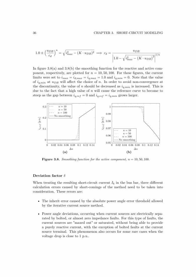
In figure 3.8(a) and 3.8(b) the smoothing function for the reactive and active com-ponent, respectively, are plotted for n = 10, 50, 100. For these figures, the currentlimits were set to imax = id,max = iq,max = 1.0 and iq,min = 0. Note that the valueof iq,min at uDB will affect the choice of n. In order to avoid non-convergence atthe discontinuity, the value of n should be decreased as iq,min is increased. This isdue to the fact that a high value of n will cause the reference curve to become tosteep as the gap between iq,ref = 0 and iq,ref = iq,min grows larger.

0 0.02 0.04 0.06 0.08 0.1 0.12 0.14

0

0.1

0.2

0.3

∆u

i q,ref

[p.u.]

n = 10n = 50n = 100

No smoothing

(a)

0 0.02 0.04 0.06 0.08 0.1 0.12 0.140.95

0.96

0.97

0.98

0.99

1

∆u

i d,ref

[p.u.]

n = 10n = 50n = 100

No smoothing

(b)

Figure 3.8. Smoothing function for the active component, n = 10, 50, 100.

Deviation factor δ

When treating the resulting short-circuit current Ik in the bus bar, three differentcalculation errors caused by short-comings of the method need to be taken intoconsideration. These errors are:

• The inherit error caused by the absolute power angle error threshold allowedby the iterative current source method.

• Power angle deviations, occurring when current sources are electrically sepa-rated by bolted, or almost zero impedance faults. For this type of faults, thecurrent sources are "maxed out" or saturated, without being able to providea purely reactive current, with the exception of bolted faults at the currentsource terminal. This phenomenon also occurs for some rare cases when thevoltage drop is close to 1 p.u..


• Errors introduced by the smoothing function. Since the source will adjustaccording to values set by the smoothing function there will be a deviationfrom the expected reference value, which in this case, is zero.

In order to evaluate the impact of these errors on the total short-circuit currentat the fault location, the deviation factor δ is introduced. In the case of completeconvergence of each source, i.e. within the allowed error threshold, the error ofeach source will be negligible. Assume instead that each source fails to provide thespecified reference value and deviates by a considerable amount. Simply lookingat the absolute error for each source will not provide a good measurement of theaccuracy of the total short-circuit current obtained in the simulation. The errorintroduced by each source needs to be evaluated based on its relative effect on thetotal short-circuit current, to be able to make any claims about the accuracy of themethod. Consider an OWPP consisting of several FRC WTGs. Assume that eachsource converges with an absolute error of 5 % for a specific short-circuit case, andthat the short-circuit contribution from the grid is many times larger than that ofthe turbines. Simply stating that the error of the simulation is 5 % would be inac-curate, but should rather be scaled according to its effect on the total short-circuit.For instance, if the grid is very strong, while the turbines are few and of low powerrating, an error of 5 % would be negligible.

Consider the resulting short-circuit current Ik,CSiof each current source i = 1, 2, . . . , N .

The error factor of each current ξi is evaluated according to

ξi = |ejφi − ejφ∗ref,i | =

√(cos(φi)− cos(φ∗ref,i))2 + (sin(φi)− sin(φ∗ref,i))2

Here, φi is the power angle of source i obtained through simulations while φ∗ref,iis the reference value calculated by neglecting the smoothing function. The errorfactor provides a way of scaling the short-circuit current of each source to the non-linear deviation caused by the error.

Assuming that the external feeding network is contributing with a major part ofthe short-circuit current, and that this current is more or less unaffected by thecurrents provided from the turbines (this will be true in the case of bolted faults),the deviation factor δ is given by

δ =

N∑i=1

Ik,CSi(Un,CSiUn,k

)ξiM∑j=1

Ik,Qj(Un,Qj

Un,k)

(3.1)

The respective current is referred to the nominal voltage level Un,k of the short-circuited bus bar or terminal. The denominator is the sum of each short-circuitcurrent Ik,Qj

provided by any feeding network j = 1, 2, . . . ,M . Un,CS and Un,Q de-notes the nominal voltage level of the current source, and external network feeder,


respectively. The error factor introduced in the above expression provides a variableestimate of the deviation from the true or expected result. Consider, once again,the case when there is complete convergence in the method. If the error factor wasnot used to scale the source currents, the obtained deviation would not reflect thefact that the method has arrived at an expected value, but would rather provide arelationship between the total current from the grid and the turbines.

Current calculations

The relevant simulation results obtained in PowerFactory and used by the methodare I ′k, id.c., Ib and Ith. Here, the transient short-circuit current I ′k is equal to thesteady-state short-circuit current Ik. I ′k is the total short-circuit current in the busbar or terminal. The values of id.c., Ib and Ith are all calculated according to theselected calculation method in the complete method, see Section 3.2, and based onthe value of I ′k. This is due to the fact that both the transient and subtransientshort-circuit from the grid and current sources are identical. The short-circuit mod-els used for the external grid, and current source, are based on subtransient values,which will be identical to the transient and steady-state values, given that the sys-tem is meshed. Based on the recommendations in IEC 60909, Method C(1) has beenused for this project. Note, that for the calculation of impedance ratio of the grid,the current sources are left open circuit. The DC component of the short-circuitcontribution from each WTG can therefore be viewed as ignored. This is consistentwith the fast transient response of the FRC WTG controller. If one studies thesimulated transient response of different types of FRC WTGs in [8, 9, 18], the DCcomponent is seemingly close to zero. Similarly, the thermal equivalent current isalso calculated based on the exclusion of DC contribution from the current sources.

The deviation factor δ derived in the previous section is used for post-calculationof an conservative estimate of the resulting short-circuit current I ′k. This post-calculation is carried out according to

I ′k,δ = I ′k(1 + 2δ)

This value is conservative, in the sense that the original current I ′k, is increased twotimes the deviation factor. This is to account for the worst case scenario, when theerror in the current source currents completely cancels out a portion of the totalshort-circuit current. The purpose of this value is to provide an estimate of the trueshort-circuit current that would have been obtained, given that all sources convergedcompletely, while at the same time providing a certain level of conservativeness.

3.3.3 Iterative AlgorithmThe iterative algorithm implemented in PowerFactory is based on an outer and innerloop, see figure 3.9. The outer loop iterates through all available current sources in


the system and passes them to the inner loop one by one. This process is repeated,until all current sources have converged within one single iteration of the outer loop,or the maximum number of iterations have been reached. The inner loop iterativelyalters the current source parameters according to the reference values defined bythe terminal voltage drop at each source. The loop is terminated either when thecurrent source has converged to the reference values, the maximum number of innerloop iterations have been reached or the source has saturated. At the end of thealgorithm relevant values are calculated or obtained from simulation results. Intable 3.4, the basic input parameters required by the algorithm, can be found.


Outer loop

Start

Stop

Inner loopIterate through eachcurrent source until allsources have arrived atthe specified referencevalue within in one sin-gle loop

Iteratively alter thecurrent source in orderto obtain the referencereactive and active cur-rent

Input parameters

Output results

Figure 3.9. PowerFactory current source model.

Note that the iterative algorithm only serves to determine the steady-state short-circuit contribution of each turbine, as well as calculating the deviation factor δ.All other relevant quantities are obtained from PowerFactory simulation resultsand post-processed values based thereof. In the following paragraphs, the inner andouter loop algorithm are explained in more detail, using algorithm flow charts. Infigure 3.10, a description of the blocks used in this type of representation can befound.

Statement 1? and/orStatement 2?

Start(input parameters)/Stop(output parameters) Input/Output

• Perform task 1

• Perform task 2

• etc.

Subroutine(input parameters) =output parameters

Figure 3.10. Explanation of algorithm flow chart building blocks.


Table 3.4. Basic input parameters required by the iterative algorithm.

Parameter Descriptionimax Maximum total output current of the FRC WTG in p.u.

during a short-circuit.iq,max Maximum reactive current of the FRC WTG in p.u. during

a short-circuit.iq,min Optional. Minimum reactive current of the FRC WTG in

p.u. during a short-circuit. If this value is not specified, i.e.set to zero, then iq,min = k∆u.

id,max Maximum active current of the FRC WTG in p.u. during ashort-circuit.

nIter1 Maximum allowed number of iterations for the outer loop.Default value: 100

icap Initial current type setting of each current source. Defaultvalue: 1

isetp Initial current direction of each current source. Defaultvalue: -1.0

cosφ Initial power factor of each current source. Default value:0.1

φerr Absolute power angle error tolerance used in the inner loop.Recommended value: 0.05

nIter2 Maximum allowed number of iterations for the inner loop.Default value: 10

kn Nudge factor used in the inner loop. Can be increased toimprove convergence times, or decreased in the rare event ofrapid changes of reference values at the dead band voltage.Default value: 1.0.

uDB The dead band voltage is the retained voltage in p.u. at theWTG terminal at the point where the reactive current out-put of the turbine generator should be controlled accordingto the assumed grid code voltage control curve.

K Slope of the linear control region of the grid code voltagecontrol curve.

n Polynominal factor of the smoothing function. Should bedecreased if the algorithm has difficulties converging foriq,min 6= 0. Default value: 100


Inner loop

Consider the inner loop flow chart in figure 3.11. The algorithm is initialized by run-ning a short-circuit calculation and setting the counters iResOk and iMaxedOutto zero. From the initial short-circuit calculation, the bus voltage at the currentsource terminal is measured, as well as the power angle φ. Note that settings for theshort-circuit calculation, such as the fault location and fault impedance, need to besetup externally in PowerFactory under the "Short-circuit calculation"-tab. Fromthe initial short-circuit calculation, the initial reference currents are determined bythe subroutine RefCurrents. This subroutine is implemented based on the gridcode reference curve and smoothing function described in Section 3.3.2.

The resulting reference active and reactive current are used to calculate the refer-ence power angle φref . Note the minus sign appearing in the expression found infigure 3.11. The desired current fed into the grid should be inductive, i.e. the reac-tive current should be lagging the active component. Furthermore, the current setpoint is scaled according to the total reference current. At this point, the absoluteerror between the actual and reference power angle is determined. If it is belowthe threshold value φerr = |φ − φref |, the current parameter settings of the sourceis acceptable and the loop sets iResOk = 1 before it is terminated. When devel-oping this method, the error threshold was set to φerr = 0.05, which also is therecommended value. This value was selected since it provided sufficiently accurateresults, while not impeding the convergence of the method.

If the actual power angle is outside of bounds, i.e. the error threshold, the loopwill start altering the parameters of the source iteratively. The rate at which thepower angle of the source is altered is determined by ki = 1 + k and kd = 1 − k,where k is the alteration coefficient. Depending on the actual and reference powerangle, as well as the power factor of the source, k will be set according to table 3.5.As can be seen in the table, k is determined by a constant part multiplied withthe absolute difference in power angle and reference power angle |φ − φref |. Theconstant part has been determined through an iterative process, where the valueswere set in order to obtain convergence in a large amount of operation scenarios.In general, it can be noted that when the source is operated close to unity powerfactor cosφ = 1, the rate at which the source should be altered is reduced. Therelative factor |φ − φref | helps to speed up the iteration by increasing k when theerror is large, and reducing it when the method is very close to a solution.


Start(imax, iq,max, iq,min, id,max, φerr, nIter2, kn, uDB, K,n)

• Perform initial short-circuit calculation

• iResOk=iCSsat=0

• Measure u and φ at current source terminal

RefCurrents(u, imax, iq,max, iq,min,id,max, uDB, K, n) = iq,ref , id,ref

• φref = arctan(−iq,ref/id,ref )

• inewsetp =√i2q,ref + i2d,ref ·

ioldsetp

|ioldsetp|

|φ− φref | < φerr? • iResOk=1yes

Stop(iResOk,iCSsat)

• iIter2=1

• φprev = 180

no

|φ− φref | < φerroriIter2 > nIter2?

Stop(iResOk,iCSsat)yes

φ = φprev?

no

• iResOk=iCSsat=1yes

Stop(iResOk,iCSsat)• φprev = φref

• Calculate k according to table 3.5

• Apply kn and calculate ki/kd

• Alter cosφ, isetp and icap according to table 3.6

• Perform short-circuit calculation

• Measure u and φ at current source terminal

• iIter2new = iIter2old + 1

no

RefCurrents(u, imax, iq,max, iq,min,id,max, uDB, K, n) = iq,ref , id,ref

• φref = arctan(−iq,ref/id,ref )

• inewsetp =√i2q,ref + i2d,ref ·

ioldsetp

|ioldsetp|

Figure 3.11. Inner loop


Table 3.5. Alteration coefficient k

|φ− φref | |φ| cosφ k> 45 0.025 · |φ− φref |> 30 0.0025 · |φ− φref |> 5 < 60 > 0.97 0.0001 · |φ− φref |

< 0.97 0.001 · |φ− φref |> 60 0.025 · |φ− φref |

> 1 < 60 > 0.97 0.00005 · |φ− φref |< 0.97 0.001 · |φ− φref |

> 60 0.025 · |φ− φref |< 1 < 60 > 0.97 0.00002 · |φ− φref |

< 0.97 0.005 · |φ− φref |> 60 0.025 · |φ− φref |

Depending on the difference in power angle, and the quadrant in which the currentsource is operating, the current source parameters need to be set according to table3.6. These regions are implemented based on the current quadrants found in figure3.6. The column labeled "Action" provides information regarding what changes aremade to the current source parameters. These will depend on the conditions listedin the remaining columns and rows in the table. The subscript old indicates thecurrent value of the parameter, while new is the new value, calculated based onthe old one. The variable φprev is used to keep track of the cases when the reac-tive current of the source is saturated. At this point, the source parameters arechanged, but has no effect on the resulting short-circuit current (this is a conse-quence of using the Complete Method in PowerFactory). For this case, iResOk = 1and iCSsat = 1 before the loop is terminated. When the source is set to a newquadrant, the parameter φprev is set to −180. This is because the behavior of thesource will be unchanged at the boundary between two quadrants.

There are two special cases implemented in the inner loop when determining howthe source should be altered. The first one is when ki cosφold > 1. This correspondsto the case when an increase in the power factor parameter would be outside of theallowed bounds of the current source model. To amend this, cosφ is simply set to1. The other case is when kd cosφold < 0.001. In this case, the reduction of thecurrent value of cosφ will be too small to make any change, and it is simply set to0. Also, it is worth pointing out that the method only allows the source to movefrom the first quadrant to the fourth, and vice verse. During the implementation ofthe method, it was discovered that there was no need to allow the source to movein any other direction when operating in these quadrants.


Table 3.6. Adjustment of the current source. The action taken to alter thesource depends on the current quadrant in which the source is currently oper-ating, as well as the actual power angle and power factor.

Quadrant icap isetp φ cosφ Action

1st0 < 0 < φref

0 cosφnew = 0.01

1Change to 4th quadrant:icap = 1φprev = −180

- ki cosφold > 1⇒ cosφnew = 1ki cosφold ≤ 1⇒ cosφnew = ki cosφold

> φref - cosφnew = kd cosφold

2nd 1 > 0

< φref

0

Change to 1st quadrant:icap = 0φprev = −180imax = −1

- kd cosφold < 0.001⇒ cosφnew = 0kd cosφold ≥ 0.001⇒ cosφnew = kd cosφold

> φref

1Change to 3rd quadrant:icap = 0φprev = −180


3rd 0 > 0

< φref

1Change to 2nd quadrant:icap = 1φprev = −180

- kd cosφold < 0.001⇒ cosφnew = 0kd cosφold ≥ 0.001⇒ cosφnew = kd cosφold

> φref

0

Change to 4th quadrant:icap = 1φprev = −180isetp = −imax


4th 1 < 0

< φref- kd cosφold < 0.001⇒ cosφnew = 0

kd cosφold ≥ 0.001⇒ cosφnew = kd cosφold

> φref

1Change to 1st quadrant:icap = 0φprev = −180



Outer loop

Consider the outer loop flow chart in figure 3.12. The method is initialized by set-ting all current sources according to input, i.e. icap, isetp and cosφ. Note that thecurrent set point isetp will be scaled by the input parameter imax for all sources.The recommended values of icap, isetp and cosφ are found in table 3.4, and wereused in the development of this method. In each iteration of the outer loop, anattempt to converge to the reference value of each source is made using the innerloop. If a source is within the tolerance φerr at the start of the inner loop, or if it issaturated, the source will be flagged as acceptable, i.e. iResOk = 1. If all sourcesare considered as acceptable within one single loop of the iteration, the method isconsidered as completed. At this point, the deviation factor δ is calculated and dis-played along with the number of saturated sources, as well as the total simulationtime. In order to obtain fast convergence, it has been noted that it is beneficial tokeep the number of inner loop iterations relatively low, compared to the numberof outer loop iterations, when dealing with a large amount of current sources. Agreat number of inner loop iterations would result in local convergence for one ofthe sources, but at the same time have greater impact on the surrounding sources.An incremental change in each source, however, will subsequently push all sourcesto convergence simultaneously.


Start(imax, iq,max, iq,min, id,max, nIter1, i_cap, isetp, cosini, φerr, nIter2, kn, uDB, K, n)

• Initialize PowerFactory short-circuit object

• Initialize all current sources using i_cap, isetpand cosini

• nF lag = Number of energized current sources

• iF lag = iTotMaxedOut = 0

• iIter1 = 1

iF lag = nF lag? • Calculate δ according to (3.1)yes

Stop(δ, iTotMaxedOut, tsim)

iIter1 > nIter1?

no

Output: "No convergence"yes

Stop(tsim)

• iF lag = 0

• iTotMaxedOut = 0

no

InnerLoop(imax, iq,max, iq,min,id,max, φerr, nIter2, kn, uDB, K, n)= iResOk, iCSsat

iResOk = 1?• iF lagnew = iF lagold + 1

• iTotMaxedOutnew = iTotMaxedOutold +iCSsat

yes

All current sources han-dled by inner loop?

no

Repeat process for nextcurrent source

iIter1new = iIter1old + 1 yes

no

Figure 3.12. Outer loop


3.4 Wind Power Plant Aggregation ModelConsider the current source method described in the previous section. When dealingwith a system model consisting of a large number of current sources, the conver-gence time of each simulation will be relevant. By aggregating the WTG arrays inthe system, a considerably lower number of current sources could be used in model.By reducing the number of current sources handled by the iterative algorithm, theconvergence time can be improved, which is important if a great number of studiesare to be performed. For any fault occurring inside an array, a non-aggregatedrepresentation is still the only valid approach. This, however, does not prevent anyremote WTG array in the system to be aggregated. A method used for WTG plantaggregation was originally proposed in [26]. Note that this method was initiallyintended for load-flow calculations. The remainder of this section will summarizeselected parts of the method found the aforementioned article.

In figure 3.13 the generic representation of a WTG array can be found. Each WTGi is connected through a transformer Ti to a segment of the array cable. Let Zi bethe cable impedance separating WTG i from the subsequent WTG. Zn representsthe last stretch of cable connecting the array to the platform, with WTG n beingthe turbine closest to the platform. Assume that each turbine is operated at unitypower factor, i.e. Si = Pi. Furthermore, each turbine is assumed to be operatedat an equal voltage, that is V1 = V2 = · · · = Vn = V . This assumption is neverjustified in the source material. In a real system the voltage, especially the voltageangle, will differ between each turbine in an array even during rated operation, sinceall generators are separated by complex impedances.

Figure 3.13. Overview of a WTG array with n interconnected WTGs inseries.

For the following derivation, all values are assumed to be in per unit. Let the voltagedrop across the cable impedance Z1 be

∆V1 = I1Z1 = S1V

Z1 = P1V

Z1

where Ii = I1 is the current of the first WTG. The voltage drop of the second

3.4. WIND POWER PLANT AGGREGATION MODEL 49

impedance Z2 will depend on the sum of the currents of WTG 1 and 2, i.e.

∆V2 = (I1 + I2)Z2 = (P1V

+ P2V

)Z2

From the above expression, it follows that the voltage drop across the nth impedancewill be

∆Vn = (I1 + I2 + · · ·+ In)Zn = (P1V

+ P2V

+ · · ·+ PnV

)Zn

The power loss in Z1 can be written as

SLoss,Z1 = ∆V1I1∗ =

(P1V

)(P1∗

V ∗

)Z1 = P1

2

V 2 Z1 = PZ12

V 2 Z1

where PZi = PZ1 is the active power transmitted through the impedance. From thisit follows that

SLoss,Z2 = ∆V2I2∗ = (P1 + P2)2

V 2 Z2 = PZ22

V 2 Z2

and more generally

SLoss,Zn = ∆VnIn∗ = (P1 + P2 + · · ·+ Pn)2

V 2 Zn = PZn2

V 2 Zn

The total loss in the array cable can be written as the sum of the above losses

SLoss = PZ12Z1 + PZ2

2Z2 + · · ·+ PZn2Zn

V 2 (3.2)

Now consider the equivalent model found in figure 3.14. The WTGs found in figure3.13 are now replaced by a generator producing a sum of the active power generatedby each WTG in the non-aggregated model. The equivalent current Ieq flowing outof the WTG array should be equal in both the aggregated and non-aggregatedmodel.

Figure 3.14. Aggregated equivalent model of WTG array.

The voltage drop across the equivalent array cable impedance Zeq will thus be

∆Veq = IeqZeq = (P1 + P2 + · · ·+ Pn)V


since the total power transmitted through the equivalent impedance should be equalto that of the nth impedance in the non-aggregated model. This is based on the as-sumption that the power loss in each cable segment is considerably smaller than thetotal transmitted power. The power loss in the equivalent impedance is expressedas

SLoss,Zeq = ∆VeqIeq∗ = IeqIeq

∗Zeq =

=(P1 + P2 + · · ·+ Pn

V

)(P1 + P2 + · · ·+ PnV

)∗Zeq =

= (P1 + P2 + · · ·+ Pn)2Zeq

V 2 = PZn2Zeq

V 2 (3.3)

By setting (3.3) equal to (3.2) the following results are obtained

PZn2Zeq

V 2 = PZ12Z1 + PZ2

2Z2 + · · ·+ PZn2Zn

V 2

which can be rewritten as

Zeq =∑ni=1 PZi

2Zi

PZn2 (3.4)

In [26], the method for equivalencing the impedance of the aggregated WTG trans-formers, Teq, is also described. For the purpose of this project, however, there isno need for this method. The transformer model used in PowerFactory allows foraggregation of two or more parallel transformers, which is the case for a WTGarray in the above format. Similarly, the turbines can easily be aggregated, by us-ing a current source with a rated current corresponding to the equivalent current Ieq.

When using this aggregation method, one should keep in mind that it is developedfor load-flow simulations. The method can only be considered as valid for caseswhen all turbines are operated at a similar voltage. For certain operation scenarios,system configurations or high array cable impedances this may not always be thecase.

Chapter 4

Numerical Results

In this chapter two case studies are performed and evaluated. From the results,general conclusions related to the current source method, are drawn.

4.1 Case Study: Single WTG connected to a Strong Grid

4.1.1 Introduction

The purpose of the case study is to illustrate the functionality of the current sourcemethod, while also demonstrating its performance. In addition to this, the staticgenerator model in PowerFactory has been included in a test case for comparison.The case study is illustrating a single WTG connected through a transformer to astrong grid. The generating capacity of the WTG model is 100 MW, and simulatesan aggregated OWPP where cable impedances have been neglected. Note that thepurpose of the case study is not to illustrate a realistic short-circuit simulation, butrather provide a benchmark of the newly developed method.

4.1.2 Test System Overview

Consider the test system in figure 4.1(a). The FRC WTG is represented by boththe current source model and the static generator. The WTG is connected to aexternal network model through a 2-winding transformer. The external networkmodel represents a strong grid.

External network

The input parameters of the external network can be found in table 4.1. In order forthe external network to act as a strong grid, the load-flow characteristics have beenselected as a slack type with nominal voltage 1 6 0 p.u.. The choice of short-circuitpower, and impedance ratio, are depending on the strength and characteristics ofthe modeled grid. With no available information of a real life grid model, theseparameters need to be selected based on assumptions. In order to model a strong

51

52 CHAPTER 4. NUMERICAL RESULTS

W TG terminal

PCC

Static Generator

~

AC Current Source

2-W

indi

ng T

rans

form

er2-

Win

ding

Tra

nsfo

rmer

33/

0.69

kV

External Grid

DIg

SIL

EN

T

(a) PowerFactory test sys-tem overview

W TG terminal

PCC

Static Generator

~

AC Current Source

2-W

indi

ng T

rans

form

er

External Grid

DIg

SILE

NT

(b) Overview fault case 1

W TG terminal

PCC

Static Generator

~

AC Current Source

2-W

indi

ng T

rans

form

er

External Grid

DIg

SILE

NT

(c) Overview fault case 2

Figure 4.1. Overview of the case study.

grid, the Short-Circuit Ratio (SCR) needs to be considered [36]. The SCR is theratio between generated power and assumed short-circuit power of the connectedgrid. The SCR of a strong grid is discussed through out the literature and consideredto be anywhere from SCR > 2 [37] to SCR > 25 [38]. For this case study, the SCRhas been selected as 10. In other words, the short-circuit power S′′k of the externalnetwork is 1000 MVA, since the generated power is 100 MW. The impedance ratiohas been set to 0.1, in order to represent a mainly inductive grid. In accordance withthe IEC 60909 standard, the voltage factor has been set to 1.1, since the voltagelevel of the bus connection is 33 kV. By using a voltage correction factor of 1.1 thelevel of conservativeness is increased.

Table 4.1. Input parameters of the external network model.

Parameter Description Valueu Nominal voltage 1 p.u.ϕ Voltage angle 0S′′k Short-circuit power 1000 MVAr1 Impedance ratio 0.1cmax Voltage factor 1.1

2-winding transformer

The input parameters of the 2-winding transformer can be found in table 4.2. Forthis case study, the transformer winding setup is YNyn0, a Y-connection with

4.1. CASE STUDY: SINGLE WTG CONNECTED TO A STRONG GRID 53

grounded neutral at both the high and low voltage side. The transformer is op-erating at a fixed turns ratio without an OLTC. The selection of impedance isarbitrary, but in the range of what could be expected for a high power transformer.

Table 4.2. Input parameters of the 2-winding transformer model.

Parameter Description ValueSn Rated power 100 MVAUh/Ul Voltage ratio 33/0.69 kVx1 Positive sequence reactance 0.01 p.u.R/X ′′ Positive sequence resistance 0.001 p.u.

Static generator

The input parameters of the static generator can be found in table 4.3. The choiceof short-circuit power is such that the resulting subtransient short-circuit is equalto the rated current.

Table 4.3. Input parameters of the static generator model.

Parameter Description ValueSn Rated power 100 MVAcosφ Power factor 1.0P Generated active power 100 MWS′′k Short-circuit power 100 MVAR/X ′′ Short-circuit impedance ratio 0.1

Current source

The rated current of the current source is set to 83.674 kA, i.e.

In = Pn√3 · U690V

n

= 100 MW√3 · 690 V

= 83.674 kA

4.1.3 Test Cases

In order to illustrate the capabilities of the current source method, four test caseshave been developed, in order to illustrate the effect of using different method inputparameters. These can be found in table 4.4. The input parameters were arbitrarilychosen, in order to illustrate the flexibility of the developed method.Furthermore, in each test case the system has been subject to the following faults:


Table 4.4. Current source method input parameters for test case 1-4.

Test case imax iq,max id,max iq,min K uDB n

1 1.0 1.0 1.0 0 2.0 0.1 1002 1.4 1.0 1.4 0 2.0 0.1 1003 1.0 1.0 1.0 0 2.5 0.05 1004 1.1 1.1 1.0 0.4 2.0 0.1 25

• Fault 1 : Three-phase line-to-ground fault at the WTG terminal, see figure4.1(b).

• Fault 2 : Three-phase line-to-ground fault at the PCC, i.e. the connection ofthe external network, see figure 4.1(c).

In both above cases, the fault impedance |Zf | = |Rf + jXf | = Zf has been variedsuch that the voltage drop obtained at the WTG terminal is 0 < ∆u < 1. Thefault impedance ratio has been kept at fixed ratio Xf/Rf = 5. This is a seeminglyarbitrary choice, but selected in order to obtain a mainly inductive resulting short-circuit impedance, as seen from the WTG generator. In addition to this, it allowsfor comparison with previous studies [21,39].

For the sake of comparison, the static generator has been included in test case 1for both fault case 1 and 2. Note, however, that the only comparable results forthe current source method and static generator is the total short-circuit currentfor a given fault impedance |Zf |. This is a testament to the fact that no moreinformation is available to the user, as was described in Section 1.4. To make anyclaims about the active and reactive power flow of the steady-state behavior of thestatic generator, the corresponding voltage angle of the terminal needs to be known.The current angle can, however, give some hints of the behavior of the generator.

4.1.4 Comments on the ResultsThe purpose of this section is to provide some brief comments on the obtained casestudy results. For more in depth conclusions drawn from the results, see Section 4.3.

In each test case, when utilizing the current source method, the reactive and activecurrent component, deviation factor δ and simulation time is plotted as a functionof the WTG terminal voltage drop ∆u. The simulated current components areplotted against the corresponding reference curve. See figure 4.2 and 4.5 - 4.7.

Test case 1 comparison

In figure 4.2, the simulation results obtained for the current source method areavailable. As it can be seen in figure 4.2(a) and 4.2(b), the method successfully


obtains the reference values set by the grid code, in both fault cases. In figure4.2(c) and 4.2(d), the corresponding deviation factor δ simulation time are plotted,respectively.

In figure 4.3 and 4.4, the simulation results of the current source method and staticgenerator are compared for fault case 1 and 2. In figure 4.3(a) and 4.4(a), thetotal short-circuit current is plotted as a function of the fault impedance. Thecurrent source provides a constant output current for the whole range, as expected.The static generator current generator experiences a sag for the fault impedancerange corresponding to linear reactive current ramping of the current source. Thiscan be seen in figure 4.3(b) and 4.4(b). Note, that the active and reactive currentcomponent denoted with the superscript †, are not the true values, but based on thecurrent angle solely. Given the striking similarities between the current componentsfound in 4.3(b), 4.3(c), 4.4(b) and 4.4(c), the voltage angle of the static generatorterminal can be assumed to be neglectable for the full range of fault impedances.Other than the deviation in the total current, the lack of a discontinuity in i†q,StatGenis noteworthy. If i†q,StatGen in fact is close to the true value of the reactive current,then it appears as if iq,StatGen is ramped down linearly to 0. These results can beinterpreted as consistent with the grid code voltage control curve, which the currentiteration method is based upon [24]. If this indeed is the intended behavior of thestatic generator, it indicates that the current iteration method is not applicablefor the case when the FRC WTGs are used in a study based on the E.ON voltagecontrol curve, found in figure 2.5.

Current source method, test case 1 - 4

Overall, it can be concluded that the obtained results correspond to the referencevalues. There are, however, some notable deviations. As it can be seen in figure4.2(b), 4.5(a), 4.5(b), 4.6(b) and 4.7(b), the method does not converge to the correctreference value for voltage drops close to 1 p.u.. In all test cases, this is reflectedby a deviation factor close to 1 %. Note that this only occurs for the second faultcase, i.e. at the PCC.

Consider δ in figure 4.2(c) and 4.5(c) - 4.7(c). In all test cases, there is a peak in δabove 10 % for ∆u < uDB. The cause for this is the difference between simulatedvalue and the expected "real" reference value. The calculation of δ is based on areference curve without a smoothing function. This will result in an increasing dif-ference between the "real" reference value and the one obtained using the smoothingfunction, as ∆u is increased closer to uDB.

Also, the simulation time for the same voltage range mentioned is considerablyhigher, see figure 4.2(d) and 4.5(d) - 4.7(d). This is due to the fact that for voltagedrops close to uDB, the active current is at its maximum, and for this systemsetup this corresponds to a current source power factor close to 1. In the method


implementation, the incremental change of the power factor is kept small for cosφclose to 1 to avoid overshoot.


0 0.1 0.2 0.3 0.4 0.5 0.6 0.7 0.8 0.9 10

0.5

1

∆u

i q[p.u.] iq,sim - Fault 1

iq,sim - Fault 2iq,ref

(a) Reactive current component iq

0 0.1 0.2 0.3 0.4 0.5 0.6 0.7 0.8 0.9 10

0.5

1

∆u

i d[p.u.] id,sim - Fault 1

id,sim - Fault 2id,ref

(b) Active current component id

0 0.1 0.2 0.3 0.4 0.5 0.6 0.7 0.8 0.9 1−4−3−2−1

∆u

log 1

0δ

Fault 1Fault 2

(c) Deviation factor δ

0 0.1 0.2 0.3 0.4 0.5 0.6 0.7 0.8 0.9 10

5

10

15

∆u

Simulationtim

e

Fault 1Fault 2

(d) Simulation time

Figure 4.2. Current source method simulation results for test case 1.


−7 −6 −5 −4 −3 −2 −1 00.7

0.8

0.9

1

log10|Zf |

i[p.u.]

iCurrentSourceiStatGen

(a) Total short-circuit current

−7 −6 −5 −4 −3 −2 −1 00

0.5

1

log10|Zf |

i q[p.u.]

iq,CurrentSource

i†q,StatGen

(b) Reactive current component

−7 −6 −5 −4 −3 −2 −1 00

0.5

1

log10|Zf |

i d[p.u.]

id,CurrentSource

i†d,StatGen

(c) Active current component

Figure 4.3. Simulation results for test case 1 - fault 1: Comparison betweenresults obtained using the current source method and the static generator modelwith current iteration.


−3 −2.5 −2 −1.5 −1 −0.5 0 0.5 1 1.5 2 2.50.7

0.8

0.9

1

log10|Zf |

i[p.u.]

iCurrentSourceiStatGen

(a) Total short-circuit current

−3 −2.5 −2 −1.5 −1 −0.5 0 0.5 1 1.5 2 2.50

0.5

1

log10|Zf |

i q[p.u.]

iq,CurrentSource

i†q,StatGen

(b) Reactive current component iq

−3 −2.5 −2 −1.5 −1 −0.5 0 0.5 1 1.5 2 2.5−0.5

0

0.5

1

log10|Zf |

i d[p.u.]

id,CurrentSource

i†d,StatGen

(c) Active current component id

Figure 4.4. Simulation results for test case 1 - fault 2: Comparison betweenresults obtained using the current source method and the static generator modelwith current iteration.


0 0.1 0.2 0.3 0.4 0.5 0.6 0.7 0.8 0.9 10

0.5

1

1.5

∆u

[p.u.]

iq,sim - Fault 1iq,sim - Fault 2

iq,ref


0 0.1 0.2 0.3 0.4 0.5 0.6 0.7 0.8 0.9 1

0.5

1

1.5

∆u

[p.u.]

id,sim - Fault 1id,sim - Fault 2

id,ref


0 0.1 0.2 0.3 0.4 0.5 0.6 0.7 0.8 0.9 1−4

−3

−2

−1

∆u

log 1

0δ

Fault 1Fault 2


0 0.1 0.2 0.3 0.4 0.5 0.6 0.7 0.8 0.9 10

5

10

15

∆u

Simulationtim

e

Fault 1Fault 2

(d) Simulation time



0 0.1 0.2 0.3 0.4 0.5 0.6 0.7 0.8 0.9 10

0.5

1

∆u

[p.u.]

iq,sim - Fault 1iq,sim - Fault 2

iq,ref


0 0.1 0.2 0.3 0.4 0.5 0.6 0.7 0.8 0.9 10

0.5

1

∆u

[p.u.]


id,ref


0 0.1 0.2 0.3 0.4 0.5 0.6 0.7 0.8 0.9 1−4

−3

−2

−1

∆u

log 1

0δ

Fault 1Fault 2


0 0.1 0.2 0.3 0.4 0.5 0.6 0.7 0.8 0.9 105

1015

∆u

Simulationtim

e

Fault 1Fault 2

(d) Simulation time



0 0.1 0.2 0.3 0.4 0.5 0.6 0.7 0.8 0.9 10

0.5

1

∆u

[p.u.] iq,sim - Fault 1

iq,sim - Fault 2iq,ref


0 0.1 0.2 0.3 0.4 0.5 0.6 0.7 0.8 0.9 10

0.5

1

∆u

[p.u.]


id,ref


0 0.1 0.2 0.3 0.4 0.5 0.6 0.7 0.8 0.9 1−4−3−2−1

0

∆u

log 1

0δ

Fault 1Fault 2


0 0.1 0.2 0.3 0.4 0.5 0.6 0.7 0.8 0.9 105

1015

∆u

Simulationtim

e

Fault 1Fault 2

(d) Simulation time


4.2. CASE STUDY: OFFSHORE WIND POWER PLANT 63

4.2 Case Study: Offshore Wind Power Plant

4.2.1 Background Description

The purpose of the case study is to illustrate the current source method in a largertest system. The test system will be subject to several short-circuits, and theeffectiveness of the current source method, and model aggregation is evaluated. Inorder to illustrate a realistic short-circuit study, a test system based on a plausiblesystem investigated by ABB. The component parameters used within the systemare based on proposed components, but have been slightly altered due to corporatesecrecy. All results are obtained using the system model in PowerFactory and post-calculated values are based on simulation data.

4.2.2 Test System Overview

In figure 4.8, an overview of the test system model in PowerFactory, can be found.An external network model is connected at the PCC, in order to model a stronggrid connection. The onshore substation connected to the PCC utilizes two onshoretransformers. The onshore substation is connected to two offshore platforms bya land and a subsea cable. Each offshore platform utilizes two power transform-ers, which subsequently are connected to one of four WTG collection grids. Eachcollection grid is here modeled by a single array consisting of ten WTGs, with anindividual rated power of 5 MW. Note that the collection grid of an OWPP usu-ally consists of several WTG arrays. For this case study, the number of arrays percollection grid has been reduced, to provide a simpler model. With ten turbines ineach array, and four arrays in total, the OWPP therefore produces a total of 200MW.

The system is designed in a symmetrical fashion, i.e. the left and right branch asseen from the onshore substation are identical. This, of course, is not completelyrealistic, but assumed for the purpose of this case study. The WTG array is mod-eled separate from the main system. In figure 4.9, the array connection is depicted.This includes both an aggregated model of the array and a non-aggregated plant,modeled separately. For any type of fault applied upstream of the array connec-tion, i.e. anywhere in the system from the WTG array connection to the PCC,the aggregated model is used. All faults applied within the array is based on thenon-aggregated model. As an example, consider a fault applied within one of thearrays. This part of the system will use the non-aggregated model while the threeremaining arrays, which are remote to the fault location, are aggregated.

The aggregated model consists of an aggregated array cable, transformer and WTGmodel. The non-aggregated array can be found in figure 4.10. The first WTG in thearray is connected directly to the array cable found in figure 4.9, while each subse-quent model is connected in parallel through an additional segment of array cable.


To WTG collectiongrid 4




MV busbar 1

Offshore transformer 4




Breaker 1 Breaker 2

Onshore transformer 1

Onshore transformer 2

Onshore cableconnection

Offshore platform 2Offshore platform 1

Subsea platforminterconnection

Onshore substation

Breaker

Subsea cable

PCC

Land cable

DIg

SILE

NT

Figure 4.8. PowerFactory model of OWPP.

To WTGs

Array cable 1aterminal

Array cable 1a

MV busbar 1

To offshore transformer 1

Aggregated WTG 1

Aggregated transformer 1

Aggregated array cable 1

~

DIg

SILE

NT

Figure 4.9. PowerFactory model of OWPP WTG array connection.


Array cables1i and 1j


To arraycable 1a

WTG 1Transformer

WTG 10 Transformer

WTG 10 Terminal

WTG 9WTG 8WTG 7WTG 6

WTG 5WTG 4WTG 3WTG 2WTG 1

WTG 10

~

~

~

~

~

~

~

~

~

~

DIg

SILE

NT

Figure 4.10. PowerFactory model of OWPP WTG array.

Each array is placed at a distance of 2.5 km from the offshore platform, and thelength of each array cable interconnecting the turbines is 700 m. Furthermore, eachWTG is connected to the array cable through a WTG transformer. In table 4.5 and4.6, the parameter values used for the system transformers and cables, respectively,can be found. The impedance of the aggregated array cables are calculated using(3.4) found in Section 3.4. With each turbine producing P = 5 MW, the aggregatedimpedance of the array cables is calculated as follows

Zeq =∑ni=1 PZi

2Zi

PZn2 =

∑9i=1 (i · P )2Z′ + (10 · P )2Z′′

(10 · P )2 =

= 0.3495 + j0.4495 Ω/km

where Z′ is the impedance of each segment of the array cable, and Z′′ is theimpedance of the array cable connecting the first WTG in the array to the platform.The parallel transformers in each array can be aggregated in PowerFactory usingthe same transformer data as the non-aggregated model. The transformer modelused for the aggregated model simply needs to be set as 10 parallel transformers inthe basic options. Each WTG is modeled using an AC current source with a ratedcurrent of 4183.69 A (non-aggregated) or 41836.9 A (aggregated). This is calculatedfrom

In,non−agg = Pn√3 · Un,WTG

= 5 MW√3 · 690 V

= 4183.69 A


In,agg = 10 · Pn√3 · Un,WTG

= 50 MW√3 · 690 V

= 41836.9 A

The external network is modeled as a slack bus with a fixed voltage of 16 0 p.u..The short-circuit behavior of the external network is modeled using the followingparameters:

• S′′k = 5000 MVA - Based on a total generated power of 200 MW (SCR = 25).

• R/X = 0.1 - Representing a mainly inductive grid.

• cmax = 1.1 - Introducing a level of conservativeness.

Note that the SCR = 25 in order to represent a very strong grid.

Table 4.5. Transformer model parameters.

Transformer Voltage rating Rated power x1 r1 TypeOnshore 400/220 kV 200 MVA 0.12 p.u. 0.002 p.u. YNyn0Offshore 220/33 kV 50 MVA 0.12 p.u. 0.003 p.u. YNyn0WTG 33/0.69 kV 5 MVA 0.08 p.u. 0.006 p.u. Dyn11

Table 4.6. Cable model parameters.

Cable Voltage rating Length X/km R/kmLand cable 220 kV 30 km 0.18 Ω 0.075 ΩSubsea cable 220 kV 40 km 0.1 Ω 0.065 ΩSubsea platform interconnec-tion

220 kV 10 km 0.1 Ω 0.065 Ω

Array cable 33 kV 2.5 km 0.1 Ω 0.06 ΩWTG interconnection cable 33 kV 0.7 km 0.1 Ω 0.1 ΩAggregated array cables 33 kV 1 km 0.4495 Ω 0.3495 Ω

4.2.3 Test CasesIn order to illustrate the behavior of the current source method, and to illustratethe short-circuit contribution from multiple FRC WTGs, several test cases havebeen developed for the case study.

First, a load-flow simulation and short-circuit calculation is performed, in orderto verify the accuracy of the aggregated impedance model used for the aggregatedWTG array. For the load-flow simulation, all current sources, both aggregated andnon-aggregated, are set according to the following parameters:

• isetp = −1


• icap = 0

• cosφ = 1

Using these settings, each source will generate a load-flow current correspondingto the rated active power of each WTG. The short-circuit calculation is performedfor a bolted fault applied directly to the WTG array connection seen in figure 4.9.Both of the above cases are considered for a system operating according to a normaloperation scenario (scenario 1) which is explained below.

Secondly, fault cases in which a bolted fault is applied at one of the following busbarsare considered:

• Fault case 1: PCC - 400 kV busbar interconnecting the OWPP to the externalnetwork, see figure 4.8.

• Fault case 2: Onshore cable connection - Low voltage side of onshore substa-tion (220 kV), see figure 4.8.

• Fault case 3: Offshore platform 1 - High voltage side of offshore platform 1(220 kV), see figure 4.8.

• Fault case 4: MV busbar 1 - Medium voltage side of offshore platform 1 (33kV), see figure 4.8 or 4.9.

• Fault case 5: Array cable 1a terminal - Connection point at the end arraycable 1a (33 kV), see figure 4.10.

• Fault case 6: WTG Terminal 10 - Terminal of WTG 10 (0.69 kV), see figure4.10.

Furthermore, for each test case the system is operated according to the two followingscenarios

• Scenario 1: Normal operation - Onshore transformer 1 and 2 are both con-nected to reduce transmission losses. The subsea platform interconnection isdisconnected and both breaker 1 and 2 are open. In other words, each trans-former in the system is operated at half the rated power, i.e. the offshoretransformer at 100 MW and onshore transformer at 200 MW. This scenariois depicted in figure 4.8.

• Scenario 2: Contingency operation - This scenario illustrates the case whenthe short-circuit impedance of the system is at its lowest. Both onshore trans-formers are still connected. The subsea platform interconnection is connectedreducing the effective impedance between the offshore platforms and the landconnection by half. Also, both breaker 1 and 2 are closed thus reducing theeffective offshore transformer impedance by half.


For the calculation of id.c. and Ith the break time t = 0.1 s and fault clearing timeTk = 1 s were used.

4.2.4 Results

All short-circuit simulation results were obtained using the algorithm input parame-ters listed in table 4.7. In each fault case, the fault location was selected accordingly,and the fault impedance Zf was kept at 0 Ω. All current components, other thanthe transient/steady-state short-circuit current, was calculated using Method C(1).

Table 4.7. Algorithm input parameters used in case study 2.

imax iq,max iq,min id,max nIter1 icap isetp1.0 1.0 0.0 1.0 100 1 1cosφ φerr nIter2 kn uDB K n

0.1 0.05 10 1.0 0.1 2.0 100

To WTGs


Array cable 1a

MV busbar 1


Aggregated WTG 1



Ul 32,808 kVu 0,994 p.u.

phiu 8,745 deg

Ul 32,618 kVu 0,988 p.u.

phiu 8,046 deg

Ul 0,000 kVu 0,000 p.u.

phiu 0,000 deg

Ul 0,000 kVu 0,000 p.u.

phiu 0,000 deg

P -49,163 MWQ 5,032 Mvar

I 0,875 kAi 0,8748 p.u.

phii -166,110 deg

P 49,508 MWQ -4,458 Mvar

I 0,875 kAi 0,8748 p.u.

phii 13,890 deg

~

P 0,000 MWQ 0,000 Mvar

I 0,000 kAi 0,0000 p.u.phii 0,000 deg

P 0,000 MWQ 0,000 Mvar

I 0,000 kAi 0,0000 p.u.

phii 0,000 deg

P 0,000 MWQ 0,000 Mvar

I 0,000 kAi 0,0000 p.u.

phii 0,000 deg

P 0,000 MWQ 0,000 Mvar

I 0,000 kAi 0,0000 p.u.phii 0,000 deg

P 0,000 MWQ 0,000 Mvar

I 0,000 kAi 0,0000 p.u.

phii 0,000 deg

DIg

SIL

EN

T

(a) Non-aggregated model

To WTGs


Array cable 1a

MV busbar 1


Aggregated WTG 1



Ul 0,000 kVu 0,000 p.u.

phiu 0,000 deg

Ul 32,618 kVu 0,988 p.u.

phiu 8,046 deg

Ul 0,694 kVu 1,005 p.u.

phiu 43,890 deg

Ul 33,083 kVu 1,003 p.u.

phiu 9,313 deg

P 0,000 MWQ 0,000 Mvar

I 0,000 kAi 0,0000 p.u.phii 0,000 deg

P 0,000 MWQ 0,000 Mvar

I 0,000 kAi 0,0000 p.u.

phii 0,000 deg

~

P -50,266 MWQ -0,000 Mvar

I 41,837 kAi 1,0000 p.u.

phii -136,110 deg

P -49,966 MWQ 4,000 Mvar

I 0,875 kAi 1,0000 p.u.

phii -166,110 deg

P 50,266 MWQ 0,000 MvarI 41,837 kAi 1,0000 p.u.

phii 43,890 deg

P -49,164 MWQ 5,032 Mvar

I 0,875 kAi 0,8748 p.u.

phii -166,110 deg

P 49,966 MWQ -4,000 Mvar

I 0,875 kAi 0,8748 p.u.

phii 13,890 deg

DIg

SIL

EN

T

(b) Aggregated model

Figure 4.11. Load-flow results for the non-aggregated and aggregated arraymodel.


To WTGs


Array cable 1a

MV busbar 1


Aggregated WTG 1



Ul 0,442 kVu 0,013 p.u.

phiu -128,518 deg


idc 0,975 kAIb 9,097 kAIth 9,284 kA

Ul 0,000 kVu 0,000 p.u.

phiu 0,000 deg

Ul 0,000 kVu 0,000 p.u.

phiu 0,000 deg


phiiks -7,554 degphiui 7,554 degP -0,000 MWQ -0,000 Mvar


Iks 0,875 kAphiiks 172,446 degphiui 59,036 deg

P 0,344 MWQ 0,574 Mvar

~


phiiks 0,000 degphiui 0,000 degP 0,000 MWQ 0,000 Mvar


phiiks 0,000 degphiui 0,000 degP 0,000 MW

Q 0,000 Mvar



Q 0,000 Mvar





DIg

SIL

EN

T

(a) Non-aggregated model

To WTGs


Array cable 1a

MV busbar 1


Aggregated WTG 1



Ul 0,000 kVu 0,000 p.u.

phiu 0,000 deg


idc 0,975 kAIb 9,097 kAIth 9,284 kA

Ul 0,071 kVu 0,103 p.u.

phiu -79,910 deg

Ul 0,863 kVu 0,026 p.u.

phiu -135,420 deg





Q 0,000 Mvar

~


phiiks 22,446 degphiui -102,357 deg

P -1,102 MWQ -5,032 Mvar


phiiks -7,554 degphiui -127,866 deg

P -0,802 MWQ -1,032 Mvar

Ikss 41,837 kAphii -157,554 deg


phiui 77,643 degP 1,102 MW

Q 5,032 Mvar


phiiks -7,554 degphiui 7,554 degP -0,000 MWQ -0,000 Mvar


Iks 0,875 kAphiiks 172,446 degphiui 52,134 deg

P 0,802 MWQ 1,032 Mvar

DIg

SIL

EN

T

(b) Aggregated model

Figure 4.12. Short-circuit calculation results for the aggregated and non-aggregated array model.

Impedance aggregation model

In figure 4.11(a) and 4.11(b), the load-flow results obtained for the non-aggregatedand aggregated array can be found. For both cases, the same bus voltage andequivalent current in the array cable are obtained. Note that the relevant resultbox used for comparison of transmitted power and current is the red box positionedclosest to the green busbar at the top. The power flow P and Q are here definedas flowing into the array cable, and it can be seen in both cases, that the deliveredpower at this node is 49.974 MW at a voltage of 1.005 p.u. and current of 0.8748 p.u..

Similar to the above case, the short-circuit results used for comparing the non-aggregated and aggregated array models can be found in figure 4.12(a) and 4.12(b),respectively. Here, the resulting transient short-circuit current in the busbar, aswell as id.c., Ib and Ith are equal in both cases. As it can be seen in the figure,the resulting short-circuit current produced by the non-aggregated and aggregatedWTG array are equal.


Fault cases

In table 4.8-4.13, the results obtained for each WTG in fault case 1 - 6 are listed.In each scenario, the resulting terminal voltage u is reported, along with the corre-sponding reactive current reference value iq,ref , the simulated reactive current iq,simand the absolute error between the two, iq,err = |iq,sim − iq,ref |. In table 4.14 and4.15 the results obtained for each busbar in scenario 1 and 2 are displayed. Here,the transient short-circuit current I ′k corresponding to the steady-state current isdisplayed. In addition to this, the following results are provided:

• Conservative estimate of the total short-circuit current I ′k,δ. This value ispost-calculated based on the obtained value of I ′k and δ.

• Decaying DC component id.c..

• Symmetrical breaking current Ib.

• Thermal equivalent current Ith.

• Deviation factor δ.

• Simulation time t.

The results for fault case 6 were obtained using kn = 0.9. The nudge factor wasapplied to decrease the incremental change in between iterations, since a problemwith convergence was detected.

As can be seen in table 4.8 and 4.9, there is no difference in the obtained resultsfor scenario 1 and 2 for fault case 1 and 2. This is because the OWPP is separatedinto two symmetrical systems, i.e. the contingency in scenario 2 does not affectthe resulting voltage drop on each WTG terminal. The maximum error obtainedwhen using only aggregated source models is obtained for fault case 4, scenario 2.This can be seen in table 4.11. Here, the error for the aggregated arrays locatedclosest to the fault location is 2.3 %. This is reflected by δ = 2.7 %, found in table4.15. Note that this is the most severe deviation obtained from all of the simulationresults. With a deviation factor of 2.7 %, the conservative estimate I ′k,δ is therefore5.4 % larger than the simulated total short-circuit current.

In table 4.13, another noteworthy result can be found. For scenario 1, numerouscurrent sources are operated at a voltage drop very close to the dead band voltage.Because of the smoothing function introduced in Section 3.3.2, a large error isincreased where the largest amounts to 17.9 %. When studying the results in table4.14, for the same fault case, one can note that even though the fault is quite severefor a number of sources, the overall deviation factor δ is 1.8 %. This deviation is inother words lower than what was obtained in the worst case results for fault case 4,scenario 2.


Table 4.8. Simulation results for a bolted fault at the PCC (fault case 1),during normal operation (scenario 1) and contingency operation (scenario 2).All values are in p.u..

Scenario 1 Scenario 2Source u iq,ref iq,sim iq,err u iq,ref iq,sim iq,err

Agg. WTG 1 0.243 1.000 0.990 0.010 0.243 1.000 0.990 0.010Agg. WTG 2 0.243 1.000 0.990 0.010 0.243 1.000 0.990 0.010Agg. WTG 3 0.243 1.000 0.990 0.010 0.243 1.000 0.990 0.010Agg. WTG 4 0.243 1.000 0.990 0.010 0.243 1.000 0.990 0.010

Table 4.9. Simulation results for a bolted fault at the onshore cable terminal(fault case 2), during normal operation (scenario 1) and contingency operation(scenario 2). All values are in p.u..



Table 4.10. Simulation results for a bolted fault at the offshore platform 1busbar (fault case 3), during normal operation (scenario 1) and contingencyoperation (scenario 2). All values are in p.u..




Table 4.11. Simulation results for a bolted fault at the MV busbar 1 (fault case4), during normal operation (scenario 1) and contingency operation (scenario2). All values are in p.u..



Table 4.12. Simulation results for a bolted fault at the array cable 1a terminal(fault case 5), during normal operation (scenario 1) and contingency operation(scenario 2). All values are in p.u..


WTG 1 0.080 1.000 0.997 0.003 0.080 1.000 0.997 0.003WTG 2 0.086 1.000 0.991 0.009 0.086 1.000 0.991 0.009WTG 3 0.091 1.000 0.985 0.015 0.091 1.000 0.985 0.015WTG 4 0.094 1.000 0.981 0.019 0.094 1.000 0.981 0.019WTG 5 0.096 1.000 0.978 0.022 0.096 1.000 0.978 0.022WTG 6 0.083 1.000 0.994 0.006 0.083 1.000 0.994 0.006WTG 7 0.089 1.000 0.988 0.012 0.089 1.000 0.988 0.012WTG 8 0.093 1.000 0.983 0.017 0.093 1.000 0.983 0.017WTG 9 0.096 1.000 0.979 0.021 0.096 1.000 0.979 0.021WTG 10 0.097 1.000 0.977 0.023 0.097 1.000 0.977 0.023Agg. WTG 2 0.762 0.476 0.476 0.000 0.294 1.000 1.000 0.000Agg. WTG 3 0.840 0.320 0.320 0.000 0.699 0.602 0.601 0.001Agg. WTG 4 0.840 0.320 0.320 0.000 0.699 0.601 0.602 0.001


Table 4.13. Simulation results for a bolted fault at the WTG 10 terminal(fault case 6), during normal operation (scenario 1) and contingency operation(scenario 2). All values are in p.u..


WTG 1 0.901 0.000 0.107 0.107 0.914 0.000 0.001 0.001WTG 2 0.900 0.000 0.135 0.135 0.911 0.000 0.001 0.001WTG 3 0.900 0.000 0.179 0.179 0.906 0.000 0.001 0.001WTG 4 0.897 0.206 0.205 0.001 0.902 0.000 0.021 0.021WTG 5 0.892 0.217 0.217 0.001 0.901 0.000 0.088 0.088WTG 6 0.901 0.000 0.119 0.119 0.913 0.000 0.001 0.001WTG 7 0.900 0.000 0.155 0.155 0.909 0.000 0.001 0.001WTG 8 0.900 0.201 0.200 0.001 0.904 0.000 0.005 0.005WTG 9 0.895 0.211 0.212 0.001 0.901 0.000 0.051 0.051WTG 10 0.000 1.000 1.000 0.000 0.000 1.000 1.000 0.000Agg. WTG 2 0.968 0.000 0.001 0.001 0.937 0.000 0.001 0.001Agg. WTG 3 0.978 0.000 0.000 0.000 0.970 0.000 0.001 0.001Agg. WTG 4 0.978 0.000 -0.001 0.001 0.970 0.000 0.001 0.001

Table 4.14. Short-circuit calculation results for all short-circuited busbars andterminals (fault case 1-6), during normal operation (scenario 1).

Fault location I ′k [kA] I ′k,δ [kA] id.c. [kA] Ib [kA] Ith [kA] δ t [s]PCC 6.561 6.642 0.401 6.561 6.672 0.006 3Onshore cableconnection

4.982 5.169 1.383 4.982 5.143 0.019 2

Offshore plat-form 1

3.653 3.732 0.019 3.653 3.687 0.011 3

MV busbar 1 9.097 9.486 0.975 9.097 9.284 0.021 5Array cable 1aterminal

7.995 8.294 0.150 7.995 8.094 0.019 13

WTG 10 ter-minal

48.321 50.065 2.107 48.321 49.060 0.018 142


Table 4.15. Short-circuit calculation results for all short-circuited busbars andterminals (fault case 1-6), during normal operation (scenario 2).

Fault location I ′k [kA] I ′k,δ [kA] id.c. [kA] Ib [kA] Ith [kA] δ t [s]PCC 6.561 6.642 0.401 6.561 6.672 0.006 4Onshore cableconnection

4.982 5.169 1.383 4.982 5.143 0.019 2

Offshore plat-form 1

4.079 4.170 0.100 4.079 4.133 0.011 4

MV busbar 1 14.324 15.112 1.751 14.324 14.634 0.027 5Array cable 1aterminal

12.465 12.795 0.114 12.465 12.597 0.013 16

WTG 10 ter-minal

49.308 49.772 2.095 49.308 50.057 0.005 36

4.3. CONCLUSIONS 75

4.3 Conclusions

From the obtained results in case study 1 and 2, it can be noted that the devel-oped current source method provides results with reasonably low deviation fromthe expected value. A maximum deviation factor of 2.7 % was obtained in faultcase 4, scenario 2. This is corresponding to a bolted fault applied at the MV busbarof the left branch in the system. One should keep in mind that there is alwaysa level of interpretation involved when analyzing the simulation results, as well asunderstanding the arbitrary relative deviation measured by δ. As an example, con-sider the worst case performance of the method in fault case 4, scenario 2. Here,the bolted fault has separated the left branch of the OWPP from the right. Theshort-circuit current from the grid, as well as the aggregated WTGs of the rightbranch, are unaffected by the short-circuit current of the left branch. Because ofthis separation of the system, the results obtained for the right branch can be seenas locally converged, in the sense that a change of the short-circuit current in theleft branch would have no effect on the right branch currents. The expected reactiveshort-circuit currents of the left branch WTGs are with most certainty 1.0 p.u., con-sidering the extremely low terminal voltages. If the reactive short-circuit currentin fact would converge to 1.0 p.u., the terminal voltage of the WTGs would in-crease. The change, however, would not alter the reference value, given the alreadyextreme voltage sag. The expected reference value for a fully converged simulationcould therefore be assumed to remain at 1.0 p.u.. Since this behavior generally onlyoccurs for cases with extremely low terminal voltages, it therefore makes sense torefer to an expected reference value. This is, in other words, not a deterministicfeature of the method, but rather based on the correlation between convergenceissues and very low terminal voltages.

From the results in case study 1 and 2, one can also detect the effect of the smooth-ing function introduced by the current source method. Once again, the simulationresults need to be interpreted by the user. The deviation caused by the smoothingfunction is measured using the deviation factor δ. Compared to the case mentionedin the above paragraph, it is much harder to make any claims about a true ex-pected value for simulation results, such as the ones found in fault case 6, scenario1. Consider the very narrow range of the reference curve for which these results areobtained. An incremental change in any of the sources could cause the referencevalue for any of the adjacent WTGs to change, to either side of the dead band.If the deviation factor for this case is compared to the worst case value obtainedin fault case 4, scenario 2, it is lower. Since the deviation factor calculated in theworst case scenario is based on truly expected reference values, as explained above,it is of higher significance. This indicates that the estimated deviation occurringbecause of the smoothing function still is less, as compared with the worst case,even though it is not based on a true reference value. Overall, it can be concludedthat the major source of error in the method is due to the saturation of the currentsources, rather than the smoothing function.


The aggregated impedance model was shown to match the non-aggregated modelwith sufficient accuracy. One has to bear in mind that these results will dependon different fault scenarios, as the aggregated model is far from a perfect descrip-tion of the system. Even though the aggregated model is effective for almost allrelevant simulation cases, it can introduce high simulation errors because of thesmoothing function used in the current source method. Once again, consider theresults obtained for fault case 6, scenario 1. Here it was shown that even though anumber of individual non-aggregated WTGs had large errors, the overall effect wasrelatively small. Instead, assume that the same terminal voltage was obtained whenusing an aggregated model, i.e. very close to 0.900 p.u.. The estimated error inthe simulation results would then be higher, given that the aggregated WTG modelcontributes with a much higher short-circuit current, as compared to a handful ofnon-aggregated turbines. In the event of such a case, the simulation would have tobe repeated with the aggregated model replaced by the non-aggregated. Since thenon-aggregated turbines are separated by array cable impedances, the result wouldbe closer to what is observed in fault case 6, scenario 1, thus mitigating the effect.

When comparing the results obtained in case study 1 and 2, it is clear that the overallsystem design will affect the simulation results. The choice of system impedances,as well as the strength of the external grid will have great impact on the level ofshort-circuit current and deviation factor δ.

Chapter 5

Final Remarks

In this chapter, a brief summary of the thesis is provided, as well as some generalconclusions and recommendations. Lastly, possible future studies within the projectare discussed.

5.1 Summary

In the process of designing offshore wind power plants, there are numerous studiesthat need to be performed. One of these studies are short-circuit studies. Duringa short-circuit, the system is subject to a sudden increase in current, due to a re-duction of impedance. The short-circuit current will, depending on the duration ofthe fault, affect the system in different detrimental ways. Short-circuit studies areimportant since they are crucial for the dimensioning of transformers and break-ers in the system. In order to be able to analyze numerous fault locations, andsystem configurations, so called static or steady-state short-circuit calculations areperformed. These studies are approximate, as compared to more precise dynamicsimulations. The benefit, however, is that they can be performed for a large numberof test cases, with significantly less effort. There are a number of industry standardsgoverning the calculation methods used for steady-state short-circuit studies.

Depending on the type of wind turbine generator utilized in the offshore wind powerplant, the short-circuit contribution will be different. One type of such turbines areso called fully-rated converter wind turbine generators. These turbines are ableto support the system during a fault through voltage regulation. By injecting acertain amount of reactive current, the turbines reduces the voltage sag during thefault, and thus, enables a faster recovery. When performing short-circuit studies,this behavior needs to be taken into account. One major issue, however, is that thisbehavior is not covered by the industry standards mentioned above.

In this master thesis project, a method used for steady-state short-circuit calcula-tions in PowerFactory has been developed. The method aims to account for the

77

78 CHAPTER 5. FINAL REMARKS

steady-state short-circuit behavior of fully-rated converter type wind turbine gener-ators, complying with voltage control curves set by an arbitrary grid code. In orderto do so, the current source model in PowerFactory has been utilized, and a specialiterative algorithm implemented. To reduce simulation times, an aggregated windturbine array model has been investigated and implemented. Two case studies wereperformed in order to evaluate and demonstrate the method. The first case studywas a benchmark of the method, including a comparison with the current iterationmethod implemented in PowerFactory. The second case study illustrated a real-lifeshort-circuit study of an offshore wind power plant. Overall, the obtained resultsshowed a high level of accuracy, which was evaluated using a relative measurementof the deviation from the expected reference value. In general, it was concluded thatthe main source of error in simulation results were due to the inherit saturation ofthe current source, in addition to the smoothing function introduced by the method.

5.2 General Conclusions and Recommendations

In order for modern society to transition from conventional power sources, new andmore sustainable technology need to be further developed. One example of suchtechnology are wind power plants placed offshore. These power systems are underthough constraints in terms of economical profitability and operations. If the gridcode requirements of a TSO are to be met, while also providing profitable and safesystem designs, the engineer needs to refine the calculation and simulation toolsavailable. The method developed in this project is a small step towards more pre-cise system designs.

The method developed for this project sufficiently handles simulation cases with alarge group of FRC WTGs. In order to improve simulation times, multiple WTGscan be aggregated. Three types of errors have been identified in the method. Thefirst one is the error introduced by the tolerance allowed in the iterative algorithm.Given the approximate nature of the steady-state calculations performed in thisstudy, the deviations introduced by this tolerance are negligible. The second typeof error is the deviation introduced by the smoothing function, used in the refer-ence curve for the reactive current component. This effect can be mitigated by usingnon-aggregated WTG models. The third, and most severe type of error, is the devi-ation caused by the inherit saturation of the current source model in PowerFactory.For some types of short-circuit scenarios, the current sources will fail to obtain thetarget reactive current set by the reference value. This saturation normally occursfor cases when the terminal voltage of the WTG is very low. In order to evaluatethe effect of these errors, the deviation factor δ was introduced. This factor mea-sures the deviation from the expected WTG short-circuit currents relative to theshort-circuit contribution of the external grid. From simulations, it was found thatthe worst case value of δ was 2.7 % for a system resembling a realistic OWPP.

5.3. FUTURE STUDIES 79

It is recommended that the user of the current source method is familiarized withthe implications of δ, while also understanding the error sources found within themethod. The conservative estimate of the short-circuit current I ′k,δ, is provided toincrease the conservativeness of the short-circuit analysis. This estimate is scaledbased on the relative error of the short-circuit currents produced by the WTGs.With this in mind, it is worth pointing out that the estimate is based on the worstcase scenario, where a portion of the WTGs short-circuit contribution is completelycanceling out a part of the grid current. For the case mentioned in the paragraphabove, this corresponds to an increase of 5.4 % in the total short-circuit. Considerthe opposite case, where the same portion of the WTG short-circuit contribution issuperposed to the grid current. Analogous, the simulated total short-circuit currentI ′k would thus be 5.4 % higher than the "true" value. In other words, there is anerror tolerance of 2×5.2 = 10.8 % for this specific case. In general, this correspondsto 4×δ. I.e. when using the conservative estimate I ′k,δ, the user needs to be aware ofthe risk of obtaining a total short-circuit current which is 4× δ too high. Naturally,this statement will only be valid under the assumption that all other values withinthe simulation are correctly obtained.

5.3 Future Studies

In order to further develop the current source method, a number of improvementsare suggested.

The most crucial improvement to the proposed method, is to develop a more refinedshort-circuit model of the grid. Consider the fact that the grid still contributes witha major portion of the short-circuit current. If this model is inaccurate, or somehowerroneous, its impact on the total short-circuit current will be much higher than theestimated contribution of the wind turbine generators. Since the short-circuit be-havior of the WTGs is very much depending on the short-circuit current of the grid,this would also imply that the FRCWTG short-circuit contribution is faulty as well.

Naturally, the algorithm could be further tweaked, to improve simulation times andavoid cases when the nudge factor kn needs to be utilized. To enhance the method,and make it better suited for future short-circuit studies, the algorithm used for thereference voltage control curve could be further adjusted, to account for a greaterselection of arbitrary shapes, such as multiple slopes and break points.

Furthermore, more effort could be spent dealing with the other relevant currentcomponents briefly discussed in this thesis. One key component omitted from thisstudy is the peak current. There are two suggested ways to proceed. The first oneis to find a general formula through which the peak current can be post-calculated,much like what is done in the IEC 60909 standard. This formula would have to be

80 CHAPTER 5. FINAL REMARKS

fitted to results obtained through dynamic simulations. The second suggestion is toinclude other PowerFactory components, such as a voltage source or a synchronousgenerator, which possibly could capture the expected peak current behavior of agiven FRC WTG model. This would require further expansion of the iterativemethod, to incorporate additional PowerFactory models.

A greater number of steady-state short-circuit case studies could be performed inorder to validate the method, and its relative sensitivity to changes in the systemimpedances and external grid model. Since there was no real-life data available forthe external grid model in the second case study, more extensive research couldbe performed, to further validate the effectiveness of the current source method.Given the limited size of the second case study, a much larger OWPP could also beanalyzed in order to validate the method.

5.3. FUTURE STUDIES 81

In order to truly validate the method, however, numerous dynamic simulationsshould be performed. These results should be compared with results obtained whenusing the steady-state calculation method found in this project. The dynamic re-sults could also help to validate other short-circuit current components, such as thedecaying DC component, which for this study has been assumed to be zero. Also,the dynamic simulations could help to establish the peak current behavior of theFRC WTG, as mentioned above.

Acronyms

AC Alternating Current.

DC Direct Current.DFAG Doubly-fed Asynchronous Generator.DFIG Doubly-fed Induction Generator.DIgSILENT Digital SimuLator for Electrical NeTwork.DVS Dynamic Voltage Support.

FRC Fully-Rated Converter.FRC WTG Fully-Rated Converter Wind Turbine Genera-

tor.

HVAC High Voltage Alternating Current.HVDC High Voltage Direct Current.

IEC International Electrotechnical Commission.

LVRT Low-Voltage-Ride-Through.

OLTC On-Load Tap Changer.OWC Offshore Wind Connections, part of the Power

System Division at ABB.OWPP Offshore Wind Power Plant.

p.u. Per Unit.PCC Point of Common Connection.PMSG Permanent Magnet Synchronous Generator.

RMS Root Mean Square.

83

84 ACRONYMS

SCIG Squirrel Cage Induction Generator.SCR Short-Circuit Ratio.SMIB Single-Machine Infinite Bus.

TSO Transmission System Operator.

VDE Verband der Elektrotechnik Elektronik Infor-mationstechnik e.V..

WRIG Wound-rotor Induction Generator.WTG Wind Turbine Generator.

List of Symbols

icap Type of output current of the PowerFactorycurrent source model (capacative or inductive).

isetp Current set point of the PowerFactory currentsource model [p.u.].

k Alteration coefficient used in iterative algo-rithm.

φ Power angle.cosφ Power factor.

Ib Symmetrical breaking current.id.c. Decaying DC component.In Nominal WTG current.ip Peak current.I ′′

k Initial or subtransient symmetrical short-circuit current.

I ′k Transient symmetrical short-circuit current.

Ik Steady-state short-circuit current.I ′k,δ Conservative estimate of the resulting short-

circuit current.Ith Thermal equivalent current.

Ieq Equivalent WTG array current.Zeq Equivalent WTG array impedance.fc Equivalent frequency used for calculation of

the equivalent impedance Zc.Zc Equivalent impedance used for calculation of

the short-circuit peak current.

Zf Fault impedance.

85

86 LIST OF SYMBOLS

κ Factor used for calculation of short-circuit peakcurrent.

ZQ Short-circuit impedance of a network feeder.I ′′k,Q Rated subtransient short-circuit current of a

network feeder.Un,Q Nominal voltage at the connection of a network

feeder.Un Nominal voltage.kn Nudge factor used in the iterative algorithm of

the current source method.

δ Deviation factor.∆u WTG terminal voltage drop [p.u.].id Active current [p.u.].id,ref Active reference current [p.u.].imax Maximum reference current [p.u.].iq Reactive current [p.u.].id,max Maximum active reference current [p.u.].iq,max Maximum reactive reference current [p.u.].iq,min Minimum reactive reference current [p.u.].iq,ref Reactive reference current [p.u.].K Slope of voltage control reference curve.n Polynomial degree of smoothing function.uDB Dead band voltage [p.u.].ξ Error factor used for calculating δ.

Zk Equivalent short-circuit impedance of a net-work.

S′′k Subtransient short-circuit power level.uRr Rated resistive component of the short-circuit

voltage in per cent.ukr Short-circuit voltage at rated current in per

cent.

ZT Short-circuit impedance of a transformer.KT Transformer correction factor.Sn,T Transformer power rating.Un,T Transformer voltage rating referred to either

the high or low voltage side.

LIST OF SYMBOLS 87

xT Relative reactance of transformer in p.u..

cmax Voltage factor used for calculation of maximumshort-circuit current.

Bibliography

[1] European Commission, “The eu climate and energy package.”http://ec.europa.eu/clima/policies/package/.

[2] D. Gross and F. Roth, The Europe 2020 Strategy. Centre for European PolicyStudies (CEPS), 2012.

[3] K. Bruninx, D. Madzharov, E. Delarue, and W. D’haeseleer, “Impact of thegerman nuclear phase-out on europe’s electricity generation,” in European En-ergy Market (EEM), 2012 9th International Conference on the, pp. 1–10, 2012.

[4] International Energy Agency and Organisation for Economic Co-operation andDevelopment, “Chapter 7: Renewable energy outlook,” in World Energy Out-look 2012, WORLD ENERGY OUTLOOK, Organization for Economic Coop-eration & Development, 2012.

[5] L. Wang, J. Wei, X. Wang, and X. Zhang, “The development and prospect ofoffshore wind power technology in the world,” in World Non-Grid-ConnectedWind Power and Energy Conference, 2009. WNWEC 2009, pp. 1–4, 2009.

[6] C. Bak, “Power system technical performance issues related to the applicationof long hvac cables,” Electra, vol. 270, 2013.

[7] H. Polinder, J. Ferreira, B. Jensen, A. Abrahamsen, K. Atallah, and R. McMa-hon, “Trends in wind turbine generator systems,” Emerging and Selected Topicsin Power Electronics, IEEE Journal of, vol. 1, no. 3, pp. 174–185, 2013.

[8] G. Ramtharan, A. Arulampalam, J. Ekanayake, F. Hughes, and N. Jenkins,“Fault ride through of fully rated converter wind turbines with ac and dctransmission,” Renewable Power Generation, IET, vol. 3, no. 4, pp. 426–438,2009.

[9] H. Mokui, M. Mohseni, and M. A. S. Masoum, “Investigating the transientresponses of fully rated converter-based wind turbines,” in Universities PowerEngineering Conference (AUPEC), 2011 21st Australasian, pp. 1–7, 2011.

[10] International Electrotechnical Commission, IEC 60909-0: Short-circuit cur-rents in three-phase a.c. systems - Part 0: Calculations of currents, 2001. IEC60909-0:2001(E).

89

90 BIBLIOGRAPHY

[11] “Chapter 22: Short-circuit analysis,” in DIgSILENT PowerFactory v. 15 - UserManual (Online Edition), pp. 429–462, DIgSILENT GmbH, February, 2013.

[12] B. Tounsi, A. Henry, and L. Vanfretti, “Modelling and dynamic analysis ofoffshore wind farms according to the french tso grid code,” in IECON 2012 -38th Annual Conference on IEEE Industrial Electronics Society, pp. 1374–1380,2012.

[13] A. Ellis, R. Nelson, E. Von Engeln, R. Walling, J. MacDowell, L. Casey, E. Sey-mour, W. Peter, C. Barker, B. Kirby, and J. R. Williams, “Reactive powerperformance requirements for wind and solar plants,” in Power and EnergySociety General Meeting, 2012 IEEE, pp. 1–8, 2012.

[14] S. Chondrogiannis, M. Barnes, M. Aten, and P. Cartwright, “Modelling and gbgrid code compliance studies of offshore wind farms with doubly-fed inductiongenerators,” in Power Electronics, Machines and Drives, 2006. The 3rd IETInternational Conference on, pp. 22–26, 2006.

[15] M. Tsili and S. Papathanassiou, “A review of grid code technical requirementsfor wind farms,” Renewable Power Generation, IET, vol. 3, no. 3, pp. 308–332,2009.

[16] H. Guo, K. Rudion, and Z. Styczynski, “Integration of large offshore windfarms into the power system,” in Science and Technology, 2011 EPU-CRISInternational Conference on, pp. 1–6, 2011.

[17] M. Mohseni and S. Islam, “International regulations on the transient responseof large wind power plants,” in IECON 2011 - 37th Annual Conference onIEEE Industrial Electronics Society, pp. 3164–3169, 2011.

[18] E. Muljadi, N. Samaan, V. Gevorgian, J. Li, and S. Pasupulati, “Short circuitcurrent contribution for different wind turbine generator types,” in Power andEnergy Society General Meeting, 2010 IEEE, pp. 1–8, 2010.

[19] Y. Wang, J. Li, S. Hu, and H. Xu, “Analysis on dfig wind power system low-voltage ridethrough,” in Artificial Intelligence, 2009. JCAI ’09. InternationalJoint Conference on, pp. 676–679, 2009.

[20] R. J. Nelson and H. Ma, “Short-circuit contributions of full-converter windturbines,” in Power and Energy Society General Meeting, 2011 IEEE, pp. 1–4,2011.

[21] M. Valentini, “Fault current contribution from vsc-based wind turbines to thegrid,” Master’s thesis, Aalborg University, 2008.

[22] S. Chen, T. Lund, M. Zamastil, V. Akhmatov, H. Abildgaard, and B. Gellert,“Short-circuit calculations considering converter-controlled generation compo-nents,” in Energytech, 2012 IEEE, pp. 1–6, 2012.

BIBLIOGRAPHY 91

[23] Energinet.dk, Technical regulation 3.2.5 for wind power plants with a poweroutput greater than 11 kW, September 2010. 55986/10,.

[24] DIgSILENT GmbH, DIgSILENT Technical Documentation: What’s New inPowerFactory Version 14.1, August 2011.

[25] M. Pöller, “Modelling of wind generation for fault level studies,” in 1st WindIntegration Symposium, DIgSILENT GmbH, Frankfurt 2011.

[26] E. Muljadi, S. Pasupulati, A. Ellis, and D. Kosterov, “Method of equivalencingfor a large wind power plant with multiple turbine representation,” in Powerand Energy Society General Meeting - Conversion and Delivery of ElectricalEnergy in the 21st Century, 2008 IEEE, pp. 1–9, 2008.

[27] H. Li and Z. Chen, “Overview of different wind generator systems and theircomparisons,” Renewable Power Generation, IET, vol. 2, no. 2, pp. 123–138,2008.

[28] H. Polinder, “Overview of and trends in wind turbine generator systems,” inPower and Energy Society General Meeting, 2011 IEEE, pp. 1–8, 2011.

[29] F. Blaabjerg and K. Ma, “Future on power electronics for wind turbine sys-tems,” Emerging and Selected Topics in Power Electronics, IEEE Journal of,vol. 1, no. 3, pp. 139–152, 2013.

[30] F. Blaabjerg, Z. Chen, and S. Kjaer, “Power electronics as efficient interface indispersed power generation systems,” Power Electronics, IEEE Transactionson, vol. 19, no. 5, pp. 1184–1194, 2004.

[31] Z. Chen and E. Spooner, “Voltage source inverters for high-power, variable-voltage dc power sources,” Generation, Transmission and Distribution, IEEProceedings-, vol. 148, no. 5, pp. 439–447, 2001.

[32] I. Lar, M. Radulescu, E. Ritchie, and A. A. Pop, “Current control methodsfor grid-side three-phase pwm voltage-source inverter in distributed generationsystems,” in Optimization of Electrical and Electronic Equipment (OPTIM),2012 13th International Conference on, pp. 859–867, 2012.

[33] D. Lijie, L. Yang, and M. Yiqun, “Comparison of high capacity svc and statcomin real power grid,” in Intelligent Computation Technology and Automation(ICICTA), 2010 International Conference on, vol. 1, pp. 993–997, 2010.

[34] S.-F. Chou, C.-T. Lee, P.-T. Cheng, and F. Blaabjerg, “A reactive currentinjection technique for renewable energy converters in low voltage ride-throughoperations,” in Power and Energy Society General Meeting, 2011 IEEE, pp. 1–7, 2011.

[35] E.ON Netz GmbH, Grid Code for high and extra high voltage, 1st ed., 2006.

92 BIBLIOGRAPHY

[36] L. Wang, C.-J. Yeh, M.-H. Hsieh, C.-T. Wu, and C.-L. Lu, “Analysis of voltagevariations and short-circuit ratios of a large-scale offshore wind farm connectedto a practical power system,” in Power and Energy Society General Meeting(PES), 2013 IEEE, pp. 1–5, 2013.

[37] J. Feltes and B. S. Fernandes, “Wind turbine generator dynamic performancewith weak transmission grids,” in Power and Energy Society General Meeting,2012 IEEE, pp. 1–7, 2012.

[38] J. O. Tande, G. D. Marzio, and K. Uhlen, “System requirements for wind powerplants,” tech. rep., SINTEF Energy Research, november 2007.

[39] F. Iov, A. D. Hansen, P. Sørensen, and N. A. Cutululis, “Mapping of gridfaults and grid codes,” Tech. Rep. Risø-R-1617(EN), RisøNational Laboratory- Technical University of Denmark, July 2007. ISSN 0106-2840, ISBN 978-87-550-3622-2.

short-circuit contributions from fully-rated …714792/fulltext01.pdfdegree project in short-circuit...

Documents