short-term drivers of sovereign cds spreads - bcb.gov.br · as opiniões expressas neste trabalho...
TRANSCRIPT

Short-Term Drivers of Sovereign CDS Spreads
Marcelo Yoshio Takami
April 2018
475

ISSN 1518-3548 CGC 00.038.166/0001-05
Working Paper Series Brasília no. 475 April 2018 p. 1-53

Working Paper Series
Edited by the Research Department (Depep) – E-mail: [email protected]
Editor: Francisco Marcos Rodrigues Figueiredo – E-mail: [email protected]
Co-editor: José Valentim Machado Vicente – E-mail: [email protected]
Editorial Assistant: Jane Sofia Moita – E-mail: [email protected]
Head of the Research Department: André Minella – E-mail: [email protected]
The Banco Central do Brasil Working Papers are all evaluated in double-blind refereeing process.
Reproduction is permitted only if source is stated as follows: Working Paper no. 475.
Authorized by Carlos Viana de Carvalho, Deputy Governor for Economic Policy.
General Control of Publications
Banco Central do Brasil
Comun/Divip
SBS – Quadra 3 – Bloco B – Edifício-Sede – 2º subsolo
Caixa Postal 8.670
70074-900 Brasília – DF – Brazil
Phones: +55 (61) 3414-3710 and 3414-3565
Fax: +55 (61) 3414-1898
E-mail: [email protected]
The views expressed in this work are those of the authors and do not necessarily reflect those of the Banco Central do
Brasil or its members.
Although the working papers often represent preliminary work, citation of source is required when used or reproduced.
As opiniões expressas neste trabalho são exclusivamente do(s) autor(es) e não refletem, necessariamente, a visão do Banco Central do Brasil.
Ainda que este artigo represente trabalho preliminar, é requerida a citação da fonte, mesmo quando reproduzido parcialmente.
Citizen Service Division
Banco Central do Brasil
Deati/Diate
SBS – Quadra 3 – Bloco B – Edifício-Sede – 2º subsolo
70074-900 Brasília – DF – Brazil
Toll Free: 0800 9792345
Fax: +55 (61) 3414-2553
Internet: http//www.bcb.gov.br/?CONTACTUS

Non-technical Summary
This papers aims at presenting an approach for achieving one single model
specification, out of a combination of selected determinants most commonly studied in the
literature, for explaining sovereign CDS (Credit Default Swap) spreads. I find that not only
the S&P 500 variable is pervasive across the sample of 35 countries, but also that the
estimated coefficients on the S&P 500 variable are higher in magnitude for emerging markets
than developed countries.
CDS spreads are the cost of benefiting from an insurance-like contract against the
default of a government. The protection buyer pays a premium or spread on a periodic basis
and in exchange, upon the occurrence of a credit event (i.e., restructuring or moratorium), has
the right to sell the bond to the protection seller at face value. The spread is related to the
expected loss of the underlying bond: the higher the expected loss, the higher the spread.
Given the magnitude of the sovereign Credit Default Swaps (CDS) market (currently
at $1.6 trillion) and the valuable information it reveals about market expectations on the
probability of default, there is great need for gaining understanding about its determinants.
Timely measures of credit risk are important, for example, to central banks concerned with
the risk of their foreign reserves portfolios.
Results suggest that the proposed framework is worth trying for enhancing short-term
sovereign risk assessment. Moreover, Exchange Rate and Local Two-Year Yield show up as
statistically significant and with the correct signs for some important investable markets.
3
Sumário Não Técnico
Este artigo propõe uma abordagem para obter modelos explicativos para o spread de
CDS (Credit Default Swap) de país, dentre várias combinações possíveis das variáveis
econômicas e financeiras mais comumente usadas em estudos empíricos relacionados a este
tema. Os resultados permitem afirmar que o índice de ações de empresas americanas S&P 500
não só se apresenta como uma variável explicativa estatisticamente relevante para o spread de
CDS da maioria dos países, como também se observa que os spreads de países emergentes
têm maior sensibilidade à variação do índice S&P 500 que os de países desenvolvidos.
O spread de CDS soberano é similar a um prêmio de seguro contra um evento de
inadimplência associado ao título de governo subjacente. O comprador da proteção paga um
spread periodicamente, em troca do direito de vender o título pelo seu valor de face, quando
da reestruturação ou moratória de dívida, por exemplo, ao vendedor da proteção. O prêmio
pactuado entre as partes baseia-se na perda esperada do título subjacente: quanto mais alta for
essa perda, maior será o valor do spread.
Tendo em vista o tamanho do mercado de CDS soberano (atualmente em US$ 1,6
trilhões) e o valioso conteúdo informacional (probabilidade implícita de não honrar a dívida)
embutido nos spreads, observa-se a necessidade de obter maior entendimento sobre seus
determinantes. Indicadores tempestivos de risco soberano são importantes, por exemplo, para
bancos centrais que monitoram o risco de crédito do investimento de suas reservas
internacionais em dívida soberana.
Os resultados sugerem que a abordagem proposta pode ser aproveitada na melhoria do
processo de avaliação de risco soberano de curto prazo. Além disso, a taxa de câmbio e a taxa
de juros do título de governo de dois anos apresentaram-se estatisticamente significativos e
com os sinais esperados.
4
Short-Term Drivers of Sovereign CDS Spreads*
Marcelo Yoshio Takami**
Abstract
This paper presents large-scale estimated models, one for each country,
representing factors driving changes in CDS (Credit Default Swap) spreads of 35
sovereigns. I estimate the models and test their robustness using data from July
2005 to July 2016. The set of eligible explanatory variables comprises indicators
of the state of the global economy and of the domestic economic conditions, and
proxies for risk premia. I find that not only the S&P 500 variable is pervasive
across the countries, but also that the estimated S&P 500 coefficients are higher in
magnitude for emerging markets than developed countries.
Keywords: risk, credit, sovereign, CDS spreads
JEL Classification: C22, C53, C63, G32, H63, H81
The Working Papers should not be reported as representing the views of the Banco Central do
Brasil. The views expressed in the papers are those of the author and do not necessarily reflect
those of the Banco Central do Brasil.
* I am grateful to the Bank for International Settlement and, particularly, to Jacob Bjorheim and the Asset
Management Unit of the Banking Department for their infrastructure support. I thank for invaluable comments
and suggestions received from Vahe Sahakyan, Nayaran Bulusu, Joachim Coche, André Minella, Carlos Viana
and Jacob Nelson. I thank Bilyana Bogdanova for her capable research assistance. All errors are my
responsibility. **
Departamento de Riscos Corporativos e Referências Operacionais, Banco Central do Brasil. E-mail:
5
1. Introduction
Given the magnitude of the sovereign Credit Default Swaps (CDS) market (currently at
$1.6 trillion) and the valuable information it reveals about market expectations on the
probability of default, there is great need for gaining understanding about its determinants
(Alsakka et al., 2010). CDS contracts are particularly useful for a wide range of investors,
either for hedging existing exposures or for speculators who wish to take positions without the
need to maintain the reference obligation on their books. This is one reason why the market of
sovereign CDS is, in some cases, more liquid than the underlying sovereign bond market
itself.1 Moreover, CDS spreads may be monitored for gauging the market perception of the
debt sustainability of specific governments, as they provide more timely and, arguably, within
periods of crisis, more accurate, distress assessment than rating agencies, as conveyed by long
term ratings. Timely measures of credit risk are important, for example, to central banks
concerned with the risk of their foreign reserves portfolios.
To account for model uncertainty, I test different combinations of determinants (which
include both global and local factors) most typically used in the literature. Identifying the best
model separately for each country (please see Table (1) for the full list) might prove useful for
risk assessment and, eventually, for forecasting purposes. This procedure also allows us to
gain insights about the relative importance of each of the factors considered. The most
important result I find is that the S&P 500 index is contemporaneously negatively related to
the CDS spreads for most of the countries. Further, the coefficients of the S&P 500 are higher
for emerging markets than they are for advanced economies. I also conduct multiple
robustness checks, all of which confirm the main result of the paper.
It must be stressed that the proposed framework is not necessarily meant to either
predict crises or to enhance financial investment efficiency; however, it might prove useful
for supporting short-term sovereign risk assessment. This paper is closely related to
Westerlund et al. (2016) and Longstaff et al. (2011), but differs from these studies in the
following aspects: i) focus on the short term relationship between spreads and drivers; and ii)
comparing the drivers of CDS spreads in developed and emerging economies.
The paper is organized as follows: Section 2 revises the related literature; Section 3
presents a short description of the CDS market; Section 4 describes the data; Section 5
1 Arce et al. (2011) find that due to the higher liquidity of the sovereign CDS market, the sovereign bonds led the price
discovery process during the recent global financial crisis.
6
provides the empirical strategy, the results and the robustness assessment; and finally Section
6 concludes the paper.
2. Related Literature
In the spirit of Westerlund et al. (2016), I test different combinations of drivers,
instead of solely testing a specific model, for each sovereign. Applying a bootstrap-based
panel predictability test, Westerlund et al. (2016) find that the global drivers are the best
predictors. In line with this analysis, I find that the S&P 500 is statistically significant across
the board.
This paper’s results are also closely in line with Longstaff et al. (2011), who find that
sovereign credit spreads are primarily driven by global macroeconomic forces and that the
risk premium represents about a third of the credit spread.2 64% of the variations in sovereign
credit spreads are accounted for by a single principal component which primarily loads on
U.S. stock, high-yield markets and volatility risk premium (proxied by the VIX index).
Instead of using principal components, this paper tries to find the subsets of explanatory
variables that can best explain short-term CDS spreads for each of the countries considered.
While this paper focuses on the short-term determinants of sovereign risk, Remolona
et al. (2008) are concerned with pricing mechanisms for sovereign risk and propose a
framework for distinguishing market-assessed sovereign risk from its risk premia. They use a
dynamic panel data model with a sample covering 16 emerging countries’ sovereign CDS
spreads. In contrast, I believe that this paper provides a more comprehensive understanding of
the determinants of credit risk, since this paper’s sample covers not only emerging countries,
but also advanced economies, summing up to 35 countries.
3. Description of the CDS market
The sovereign CDS market grew from $0.17 trillion (in terms of notional amounts
outstanding) in December 2004 to almost $2 trillion in December 2015.3 During the same
period, the credit derivatives market increased from $6 trillion to $15 trillion. Figure (1)
shows that positions in sovereign contracts have become an increasing part of the CDS market
2 Longstaff, F. et al. (2011), “How Sovereign is Sovereign Credit Risk?”. 3 Notional amounts outstanding are defined as the gross nominal or notional value of all deals concluded and not yet settled
on the reporting date. These amounts provide a measure of market size and a reference from which contractual payments are
determined in derivatives markets.
7
since December 2004, while total notional amounts outstanding in the credit derivatives
market as a whole has been declining markedly since 2007.4
CDS spreads indicate the cost of buying protection against the default of a reference
entity. The protection buyer pays a premium or spread on a periodic basis and in exchange,
upon the occurrence of a credit event (defined within the terms of a CDS contract), has the
right to sell the bond to the protection seller at face value. CDS contracts are generally
considered by market participants to be efficient and liquid instruments to mitigate credit risk.
Further, they enable credit providers to diversify exposure and expand lending capacity. The
protection seller, on the other hand, can take credit exposure over a customised term and earn
the premium without having to fund the position. The spread is related to the expected loss of
the bond: the higher the expected loss, the higher the spread. Since trades by market
participants are more frequent than ratings (re)assessments by ratings agencies, CDS spreads
is a more timely, though not necessarily more accurate, way of gauging the market perception
of credit conditions of specific entities.
Triggers for sovereign CDS contracts may be a failure-to-pay, a moratorium or a
restructuring. A failure-to-pay occurs when a government fails to pay part of its obligations in
an amount at least as large as the payment requirement after any applicable grace period. A
moratorium occurs when an authorized officer of the reference entity disclaims, repudiates,
rejects or challenges the validity of one or more obligations. A moratorium that lasts a pre-
defined time period triggers a failure-to-pay event or a restructuring. Restructuring occurs
when there is a reduction, postponement or deferral of the obligation to pay the principal;
when there is a change in priority ranking causing subordination to another obligation; or
when there is a change in currency or composition of interest or principal payments to any
currency which is not a permitted currency.
Upon default, there are two types of settlement: physical or cash. Both of them cause
the termination of the contract. In the case of the physical settlement, the protection buyer
delivers to the protection seller one of a list of bonds with equivalent seniority rights and the
protection seller pays to the protection buyer the face value of the debt. In the case of cash
settlement, the protection seller pays to the protection buyer the difference between the face
value of the debt and its current market value.
4 According to the BIS, these declines are largely due to terminations of existing contracts, by netting gross notional
outstanding through portfolio compression and clearing.
8
4. Data
The dependent variable for each of the 35 investment-class markets listed in Table (1)
is the change in its 5-year CDS spreads, with the reference obligation being a deliverable
senior dollar-denominated external debt of the sovereign. Table (2) shows descriptive
statistics for the sovereign CDS spreads of the 35 selected countries.
I select the set of global and local explanatory variables that could potentially be used
by investors and risk-managers who take short-term views on sovereign risk. The focus of this
paper is on establishing statistical relationships, and not on identifying the economic content
of the variables considered. The slope of the yield curve, for example, not only provides
indirect assessment on future tax revenues, as they are related to growth prospects through the
business cycle, but also captures the risk premia embedded in long term yields. Alternatively,
it could convey information about the state of the economy with respect to growth prospects,
risk aversion, banking system vulnerability and business cycle. In this paper, I do not take a
stand on which of these interpretations matters more for the results.
In the following, I use 500sp , vix , Slopeand oil , respectively, to refer to the S&P
500 index, VIX index, U.S. slope factor and Brent oil price index. The local factors that I
consider as presumably providing information on specific aspects related to debt
sustainability or overall risk premium are the local stock index level ( istock ), exchange rate (
ixr ), local two-year yield ( ilocalTY ), local slope factor ( ilocalSlope ), and the average of
banks’ CDS spreads (when available) of the banking system of the corresponding jurisdiction
( ibank ). Given the reasonable assumption of persistence of CDS spreads, I include the lagged
dependent variable in the regression. The description of the variables, the economic
reasoning behind their inclusion and data sources are described in detail in Table (3).
To avoid potential problems of non-stationarity of the variables in our study, I analyse
the first differences of all the variables at the weekly frequency from July 2005 to July 2016. I
perform the analysis at the weekly frequency to get a sufficient sample size. This, however,
has the drawback of making it infeasible to use other macroeconomic sovereign credit-related
factors, such as deficit/GDP, debt/GDP ratios, or foreign reserves, as explanatory variables.
These variables are available at best at a monthly frequency. I test as many as possible
econometric models for a time period encompassing the period July 2005 to October 2012.
The last 45 months (from November 2012 to July 2016) are set apart for calculating out-of-
sample goodness-of-fit statistics.
9
5. Empirical Strategy and Results
First, in order to mitigate potential multicollinearity issues, I orthogonalized the
variables most usually associated to the general economic conditions (vix, oil and stock ) to
the S&P 500.
I begin the empirical analysis by attempting to narrow down the set of variables that
could be included in the regressions, by means of the Granger-causality test (Granger, 1969).
This step is useful to reduce the computational time required for the analysis. I limit the set of
eligible local explanatory variables to only endogenous and weakly exogenous ones, as given
by the Granger-causality test. I narrow the set of variables because when estimating models
with contemporaneous independent variables, a primary concern is the endogeneity of the
regressors. For example, while weekly changes in the exchange rate may anticipate changes in
CDS spreads, it could also be argued that currency changes might arise as a consequence of
changes in CDS spreads. When associated with a negative outlook of government debt
sustainability, increases in CDS spreads might lead currency depreciation as net capital
outflows ensue. In order to mitigate such endogeneity issues, I run Generalized Method of
Moments (GMM) estimations with instrumental variables for the endogenous variables.
When the variable is set as exogenous a priori (this is the case for the global variables and the
lagged dependent variable), I simply use it as instrument for itself; for the endogenous ones, I
use their first lags as instruments. Non-exogenous and non-endogenous variables are not
considered in the model specification. Therefore, by constraining the testable model
specifications to a subset of only endogenous and exogenous variables, I can save
computational cost. Parts A and B of Table (4) show chi-squared statistics for the Granger-
Causality test, respectively: i) whether local variables anticipate changes in CDS spreads, and
ii) whether the opposite holds true. A variable is deemed eligible when it is weakly exogenous
or endogenous. Table (5) shows the subset of eligible variables for each country, i.e., the
weakly exogenous and endogenous variables marked with the labels “*” and “&”,
respectively. Let’s take the case of Italy. Their eligible variables are the global variables (
500sp , vix , Slopeand oil ), and the local variables 1ispread , ilocalTY , ilocalSlope , and
ibank . The first five variables are assumed to be exogenous a priori. Weak exogeneity is
attributed to ilocalTY and ilocalSlope , as their chi-squared statistics are significant at the 10%
level in Part A (Table (4)), while their Part B’s (Table (4)) chi-squared statistics are non-
10
significant at the 10% level. ibank is set as endogenous, as their chi-squared statistics are
significant at the 10% level in both Part A and Part B. When there is no label, the
corresponding variable is not taken as eligible. Variables labelled as “(*)” in Table (5) are set
as exogenous by assumption, i.e., the global variables and the first lag of the dependent
variable are not expected to be affected by the dependent variable in any sense.
I run the change in the weekly CDS spread over the four global factors ( 500sp , vix ,
Slopeand oil ), the lagged first difference of the corresponding CDS spread, and the local
factors chosen following Granger-causality test results. Secondly, I run the large-scale engine
in Stata (Baum, 2003) for achieving one single model for each country i, according to
equation (1):
ti
k
tkikitii
j
tjjiiti ZspreadXspread ,
5
1
,,,1,
4
1
,,, ...
(1)
where:
i = constant term for country i,
tjX , = set of global factors for week t: 500sp , vix , Slopeor oil ,
tkiZ ,, = set of local factors for country i and week t: istock , ixr , ilocalTY , ilocalSlope , or
ibank ,
ti, = error term for country i and week t.
Variable transformations are such that “rate” variables are transformed first into
absolute values, i.e., CDS spreads, originally in basis points, are divided by 10000; the other
“rate” variables are divided by 100, when originally obtained in percentage format (U.S. slope
factor, Local Short-Term Yield and Local slope factor). “Price” variables are transformed into
their logarithms: S&P 500 index, VIX index, Oil price, Local Stock Index, and Exchange Rate.
I take the first differences of the resulting variables.
In the second step, I let the algorithm selects the model specification for each country
constrained by the following pre-defined set of criteria.5 First, I require that at least one
variable with significance at the 10% level has the expected sign as in Table (3) is included in
5 The total number of models tested comprises all possible permutations of factors labelled as “(*)”, “*” or “&” in Table (5).
For example, in the case of Italy, I have a set of 8 eligible factors (Table (5)): 500sp , vix , Slope , oil , 1spread , xr , localTY
, localSlope and bank . Then, the engine is due to test as many as 2551288
8
8
7
8
6
8
5
8
4
8
3
8
2
8
1
models.
11
the model. Within the space of such models, I select the one with the highest Adjusted R2
which is statistically superior to all possible nested models.6 After testing 255 model
specifications for Italy, for instance, the engine comes out with a model comprising S&P500,
Slope, spread-1 and localTY factors, as shown in Table (6). The Italy’s S&P 500 estimator
value of -0.025 means that a 1% weekly variation of the S&P500 index would be consistent,
ceteris paribus, with a 2.5 basis points contemporaneous reduction in the Italy’s CDS spreads.
Blank cells in Table (6) mean that models including the corresponding factor are superseded
by the prevailing model specification as presented in the table; or simply that this variable is
not selected in the selection procedure . Finally, I assess the goodness-of-fit of the estimations
and their forecast accuracy.
5.1 Results
The most striking result of Table (6) is that the 500sp estimator not only shows up as
significant for most of the countries (22 out of 35), but one can also notice a remarkable
difference in sensitivity magnitudes to this global factor between emerging markets and
advanced economics. For countries where 500sp doesn’t show up as statistically significant
in the specification (Germany, Netherlands, Austria, Portugal, Denmark, Poland, Turkey,
Australia, Hong Kong, Korea, China, Mexico and Chile), different combinations of global
and local factors (oil, spread-1, xr, localTY and bank) are found by the algorithm to be their
best-fit models. Quite noticeably, vix, oil and stock, which are exactly the variables
orthogonalized against 500sp , barely show up as significant for any country’s model
specification.7 In line with the usual finding that most emerging markets and advanced
economies are typically well integrated into the global markets, no local variable shows up as
a significant driver of sovereign CDS spreads for 16 out of the 35 countries.8
The pervasiveness of 500sp is consistent with the results reported by other authors
(Longstaff et al. 2011, and Pan et al., 2008). The results in Table (6) also confirm the intuition
6 A model nests another one when the first contains the same terms as the second and at least one additional term. I use the F-
test (see Greene, 2007) for testing the null hypothesis that the more comprehensive model does not contribute with additional
information. When I reject this hypothesis at 5% significance level, then the more comprehensive model is not rejected to be
superior to the nested one. 7 The only exceptions are Austria (oil), Australia (oil) and Russia (stock). 8 France, Finland, Austria, Belgium, Slovakia, Spain, Ireland, Sweden, Czech Republic, Australia, New Zealand, Japan,
Philippines, Indonesia, Thailand and Brazil.
12
that CDS spreads of emerging market sovereigns are more sensitive to global factors than
spreads of developed countries.
That the CDS spreads of Israel, Malaysia, South Africa, Mexico, Peru, Chile and
Colombia are significantly sensitive to the exchange rate is in line with the evidence (Broner
et al. 2013, Broto et al., 2011, and Calvo, 2007) that emerging markets’ debt riskiness is
tightly linked to the dynamics of global capital flows or commodity prices.
Another interesting finding is that Portugal, Italy, Russia, Poland, Hungary, Turkey
and Colombia appear in Table (6) with local two-year yields being significant. While
Portugal’s and Italy’s short-term debts might have been eventually under rollover risk
between 2010 and 2012, as per the Eurozone debt crisis, the CDS spreads and yields co-
movements of Russia, Poland, Hungary, Turkey and Colombia are consistent with the usual
view that a large part of their higher yields is presumably related to credit risk itself. In any
case, these dynamics are arguably consistent with protection-sellers charging higher
premiums on CDS contracts with those debts as reference obligations.
The fact that bank barely shows up as significant might be due to the general
assessment that the transmission of distress from the banking sector to sovereign credit may
occur more like a structural break than gradually over time.9 It could perhaps have been
expected that increases in bank, as a stress indicator of the banking sector, could have
gradually spilled over into the risk perception of sovereign bonds. Thus, the apparent
underpricing of the spillover effect from the financial stability stance to the sovereign debt
risk during the period leading to the 2010-2012 European sovereign debt crisis can be
tentatively explained by the expectation that governments would: i) monetize their debts
(perhaps more in the case of the U.S. than for Eurozone countries), ii) wipe out defaulted
bank’s shareholders and subordinated debtholders, or iii) be simply bailed out by
economically stronger sovereigns. While not having been noticeably impacted by the global
financial crisis, Hong Kong, Korea and China are three jurisdictions where the banking sector
remained relatively stable during the 2005-2012 period and where the governments are
perceived to be very supportive of their domestic big banks. This may be the reason why, in
these three cases, the sovereign and their banking system CDS spreads tend to co-move, i.e.,
why their coefficients of the bank variable showed up as significant.
9 The only exceptions are Hong Kong, Korea and China.
13
Next, I perform a goodness-of-fit analysis and compare the contemporaneous-variable
model estimation outcomes with those of ARMA structural models and lagged explanatory
variables specifications.
The goodness-of-fit of the GMM estimations is evaluated by means of Adjusted R2,
Theil’s U1, Theil’s U2 and Percent Hit Misses (PHM) statistics. I calculate Adjusted R2s for
the in-sample period, whereas for calculating Theil’s U1, Theil’s U2 and PHM out-of-sample
statistics, I use the first two-thirds of the data for estimation and perform out-of-sample tests
on the remaining sample. Normalizing the Root Mean Squared Error by the dispersion of
actual and forecasted series or calculating the root mean squared percentage errors relative to
naïve forecast (random walk), Theil’s U1 and Theil’s U2 stand, respectively, as intuitive
assessments of forecast accuracy. PHM assesses whether the direction of the prediction is
accurate or not, i.e.:
NHitMissesPHM # .
where HitMisses# = number of times the prediction does not have the same sign as the
realized value and N = total number of observations.
It is well known that higher values of Adjusted R2 imply better model fit; however,
lower Theil’s U1, Theil’s U2 and PHM values indicate better forecasting ability.
The goodness-of-fit statistics of Table (6) suggest that emerging market economies’
models presumably show more forecasting power than the developed countries’. Sorting into
ascending (Adjusted R2) or descending order (Theil’s U1, Theil’s U2 and PHM), these
statistics confirm that countries at the bottom rows of the table, broadly comprised of
emerging market economies, are associated with better goodness-of-fit measures.
As a benchmark for this paper’s GMM estimations, Autoregressive Moving Average
(ARMA) model specifications are also estimated. The ARMA(p,q) process is estimated by
Full-Information Maximum Likelihood Estimation (FIMLE), following Box-Jenkins (1994)
and Enders (2004). I select the best model according to the following criteria: i) the AR and
MA terms are significant at the 10% level; ii) the residuals behave as a white-noise process
(all autocorrelations of the residuals should be indistinguishable from zero), iii) the model has
to have the lowest Bayesian Information Criteria (BIC) statistic, iv) it is non-degenerate, i.e.,
there are no gaps within AR or MA terms and v) when i) and ii) don’t hold, then I only take
criteria iii) and iv) into account. I use Ljung-Box (1978) Q-statistic in equation (2) at 10%
significance level for testing ii).
14
s
k
k
kTr
TTQ1
2
)()2( (2)
If Q exceeds the critical value of 2 with qps degrees of freedom, then at least
one value of kr , which is the sample autocorrelation coefficient of order k, is statistically
different from zero (I set s to 10).
Table (7) shows that the goodness-of-fit statistics (adjusted R2, Theil’s U1, Theil’s U2
and PHM) are noticeably worse than those of the respective contemporaneous model statistics
(Table (6)).
As for the lagged-factor specifications, Table (8) shows that they are noticeably less
robust than those comprising contemporaneous factors. Except for a few occurrences (10 out
of 124), the lagged-variable models’ goodness-of-fit metrics are worse than those of
contemporaneous-variable models (Table (6)). Besides, the “best-fit” lagged-variable model
specifications (which I am able to obtain for all but France, Italy, Spain and Ireland) are even
worse than those of ARMA models (Table (7)).10
5.2 Robustness Check
This subsection shows that even altering the algorithm criteria significantly (changing
the significance level of the Granger-causality test at which variables are included in the
analysis, or substituting other goodness-of-fit statistics for the Adjusted R2) or repeating the
analysis across different sub-periods do not give rise to results substantially challenging this
paper’s two main claims, i.e., that the S&P 500 index is statistically significant and
contemporaneously negatively related to the CDS spreads for most of the countries, and that
emerging market’s coefficients on the S&P 500 variable are higher in magnitude than those of
advanced economies. To be sure, the S&P 500 coefficient’s statistical significance and its
magnitude do change when modifying the algorithm criteria or the sample period, leading to
different country ranking orders. The coefficient on the S&P 500 for Russia (statistically
significant and with the expected negative sign in Table (6)), for instance, is not available in
the July 2005-June 2010 and January 2008-December 2010 sub-periods’ models, while
ranging from -0.073 to -0.028 as for the other four sub-periods (Table (15) and Table (16)).
10 The ARMA-model statistics are better in comparison to the corresponding lagged model (Table (8)) in 88 out of 124
goodness-of-fit statistic values.
15
Although the individual coefficient estimates somewhat vary between the different
specifications, those of the S&P 500 remain higher (in absolute terms) for emerging markets.
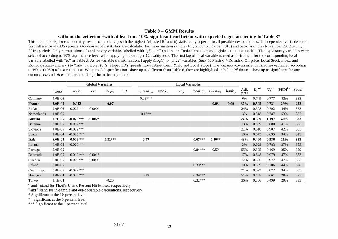
Interestingly, eliminating the criterion i) (choosing models with at least one coefficient
significant at the 10% level with the expected sign) altogether from the algorithm, or
modifying the restriction ii) (choosing models with the highest Adjusted R2), the engine still
generates models (see Tables (9) to (12)) with statistically significant negative coefficients on
the 500sp variable, higher in absolute terms for emerging market countries than for
advanced economies. Table (9) shows that the characteristics of the sole six (out of 35
models; highlighted in bold) models which happen to be distinct from those of Table (6) don’t
lead to a different assessment regarding the coefficient of the 500sp variable. By the same
token, no dramatic changes take place regarding the quantity and the magnitude of
statistically significant 500sp coefficients. It continues to play a dominant role in explaining
the CDS spreads in nearly all of our sample countries, with higher sensitivity of emerging
markets to this variable, when substituting other goodness-of-fit statistics for the Adjusted R2
as a criterion for selecting the best-fit models (Tables (10) to (12)).
Aiming to evaluate, to a fairly large extent, whether changing the Granger-causality
test significance level from 10% to 5% would lead to the rejection of this paper’s main claims,
I ran the algorithm over the six sub-periods: i) July 2005 to October 2012, ii) July 2005 to
June 2010 (Before Jul 2010), iii) July 2010 to June 2014 (After Jul 2010), iv) July 2005 to
June 2008 (Before Jul 2008), v) January 2008 to December 2010 (Subprime Crisis), and vi)
July 2010 to June 2013 (Euro Crisis). As it turns out, had I imposed a stricter cutoff (a 5%
significance level, instead of 10%), it wouldn’t materially have changed this paper’s main
outcomes.
Changing the significance level to 5% reduces the set of eligible variables either by
excluding previously selected variables, or by switching previously endogenous variables to
weakly exogenous ones. As expected, supressing previously elected variables from the set of
eligible variables leads to the algorithm generating a different model. For instance, when
excluding the LocalTY factor from the set of eligible variables, Portugal’s alternative model
(Table (14)) ends up presenting a statistically significant S&P 500 estimator, when it was not
the case previously (Table (6)). Less obviously, when the changed cutoff of the level of
significance switches a previously endogenous variable into a weakly exogenous one using
the Granger-causality test, the algorithm may prefer a different model. The Netherlands’
alternative model (Table (14)), for example, shows a statistically significant coefficient on the
16
S&P 500, when the previously endogenous variable localSlope (at the 10% significance level)
turns into a weakly exogenous variable (at the 5% level) and further excluding xr and localTY
from the set of eligible variables, even though none of these three variables were part of the
originally selected model (see Table (6)). As it turns out, this unintended consequence is due
to the change in the instrumental variables setting: endogenous variables are transformed into
lags when running the GMM regressions, while weakly exogenous ones are not.
Jointly, the results of Table (15) and Table (16) show that the net effect of reducing
the significance level from 10% to 5% in the Granger-causality test is almost neutral in terms
of the quantity of statistically significant coefficients of the S&P 500 within each sub-period.
What is more, the algorithm’s outcomes still provide support to this paper’s two main
findings. Table (15) and Table (16) also show that the differences between the quantities of
statistically significant S&P 500 estimators across the six sub-periods aren’t large: 5, 1, 0, 0, 0
and 2 out of 35 countries, respectively, for the sub-periods July 2005-October 2012 , Before
July 2010, After July 2010, Before July 2008, Subprime Crisis and Euro Crisis. Overall,
whether or not the S&P 500 is selected by the algorithm does depend on the specific setting.
Let’s take the models for New Zealand and the Colombia for the July 2005-June 2010 period
(“Before Jul 2010” column in Table (16)).11
Supressing localSlope from the set of eligible
variables for New Zealand gives rise to an alternative model where the previously non-
significant coefficient of the S&P 500 (see the corresponding column in Table (15)) now
becomes statistically significant. In contrast, the S&P 500 is no longer selected by the
algorithm for Colombia, when the Granger-causality test leads to the exclusion of the variable
stock from the set of eligible variables. Quite conspicuously, apart from slight differences in
other factor estimators for just three countries, the statistical significance of the coefficients of
the S&P 500 are pretty much the same for the July 2005 to June 2008 period (“Before Jul
2008” column in Table (15) and Table (16)).12
Ordering Adjusted R2 statistics from low to high values and the other goodness-of-fit
statistics (Theil’s U1, Theil’s U2 and PHM) the other way around (descending) according to
the column “After Jul 2010”, Table (17) and Table (20) support the finding that emerging
markets model specifications (mostly at the bottom rows of the tables) tend to show better
goodness-of-fit and forecast accuracy statistics as a group than advanced economies across all
the different sub-periods.
11 The corresponding complete model specifications are not shown, but are available at request. 12 Even generating different models for Hungary, Israel and Colombia, their S&P500 estimators differ by less than 5%.
17
Table (21) and Table (22) show respectively that ARMA models’ and lagged-variable
models’ goodness-of-fit statistics are mostly superseded by the contemporaneous models
across the other five sub-periods as they are for the July 2005-October 2012 period.13
However, comparing Table (21) values particularly with those of Table (18) and Table (19),
we find a couple of better ARMA Theil’s U1 values (highlighted in bold in Table (21),
column “Before Jul 2008”) and Theil’s U2 values (highlighted in bold in Table (21), columns
“After Jul 2010” and “Euro Crisis”); yet this is the case for just less than half the number of
countries. Showing mixed results in comparison to the corresponding ARMA-model statistics
(Table (21)) for the periods “Before Jul 2010”, “After Jul 2010”, “Before Jul 2008”,
“Subprime Crisis” and “Euro Crisis”, table 22 indicates that the lagged-variable model
statistics are worse than those of the ARMA models for the July 2005-October 2012 period
and noticeably worse than the corresponding contemporaneous model statistics (Tables (17)
to (20)). In addition, one can also notice that no coefficient of the S&P 500 appears to be
statistically significant for the two overlapping sub-periods “After Jul 2010” and “Euro
Crisis”.
6. Conclusion
I find that the S&P 500 is significant in explaining CDS spreads across a range of
countries, especially emerging markets. Moreover, the coefficients of Exchange Rate and
Local Two-Year Yield variables have the expected sign, and are also significant for some
important investable markets. On the other hand, variables such as VIX, Oil, Local Stock
index, Slope, Local Slope and Banking System are rarely found to be statistically significant in
explaining sovereign CDS spreads. Strikingly, goodness-of-fit and forecast accuracy are much
better for emerging markets than for developed countries. Models with contemporaneous
variables provide better statistical fitness than lagged-variable models. As for ARMA models,
except for a few occurrences, their goodness-of-fit and forecast accuracy statistics are worse
than for contemporaneous fundamental models across the board. When generating
fundamental models with lagged variables, however, the engine comes up with goodness-of-
fit statistics even worse than those of pure time series-generated models (ARMA).
If the past is any guide (so far I still believe it is!) and risk assessments are to be made
on a weekly basis, the proposed large-scale, econometric-based framework can be used as part
13 The corresponding complete model specifications are not shown, but are available at request.
18

of an early warning tool. While using this framework in practice, however, some caveats
should be kept in mind. Models with contemporaneous variables need one-week-ahead
predictions as inputs. Accordingly, the results point out that forecasting initiatives should be
focused on global variables, particularly those conveying the overall risk aversion or the
general state of the global economy, like the VIX or the S&P 500 factors. Not least, Longstaff
et al. (2011)’s advice is worth considering: as the estimation period is “characterized by
excess global liquidity, prevalence of carry trades and reaching for yield in the sovereign
market,” approaches like the one proposed in this paper should be taken with a grain of salt
when applied to periods not subject to those market forces. In addition, models based on
historical information do not necessarily unveil the true relationship between variables under
unusual circumstances, regardless of how sophisticated they are.
As for additional robustness assessments, I recommend applying randomization tests
on a selected set of explanatory variables and compare the forecast accuracy ex-post. For
example, if 60% of predictions of changes in S&P 500 had been correct, what would have
been the value for PHM? Besides, while this paper provides some evidence for the overall
neutrality in terms of the quantity of statistically significant S&P 500 coefficients, there is an
opportunity to more extensively check the robustness of the algorithm to potential unintended
consequences when modifying the set of instrumental variables in the GMM estimation.
Finally, for future research, one could test other banking sector-related variables.
While the well-functioning of the banking sector is key to fostering the economic
development of any country, the opposite has proved so far to hold true: banking crisis can
lead to economic recession. Not as a coincidence, the factor tibank , strikes as indicating
double causality between the sovereign and its corresponding banking system CDS spreads in
almost all cases for which I could achieve data for banks’ CDS spreads, as shown in Table
(5).14
As it turns out, distresses in the banking sector, when pervasive and impacting too-
systemic-to-fail banks, as for the 2007-2009 crisis and the European debt crisis, might lead to
negative views on the debt sustainability of the corresponding jurisdiction, which would
presumably manifest themselves by increasing CDS spreads. Playing a pivotal role in paving
the way for economic growth or where having a specific mandate for guaranteeing financial
stability, central banks, as lenders of last resort, have an incentive to bailing the banking
sector out. In this paper, although using the average of banks’ CDS spreads as a proxy for the
14 The exception is Germany, for which we cannot reject that the variable bank is weakly exogenous.
19
distress in the banking sector, it didn’t show up as significant in most of the cases.15
I
conjecture that movements in Sovereign CDS spreads might not have fully captured the
dynamics of the banking sector risk, as its transmission to sovereign credit deterioration may
occur more like a structural break than continuously in time.
References
Alsakka, R., O. Gwilym. (2010) “Leads and lags in sovereign credit ratings,” Journal of
Banking and Finance 34(11): 2614-2626.
Arce, O., Mayordomo, S., and Peña, J.I. (2012) “Credit-Risk Valuation in the Sovereign CDS
and Bonds Markets: Evidence from the Euro Area Crisis,” Available at SSRN:
https://ssrn.com/abstract=1896297 or http://dx.doi.org/10.2139/ssrn.1896297 .
Baum, C. (2003) An introduction to modern econometrics using Stata. Stata Press, College
Station.
Blanchard, O. (2005) “Fiscal dominance and inflation targeting: lessons from Brazil,” In
Giavazzi, G., Goldfajn I., and Herrera S. (Eds.) Inflation targeting, debt and the Brazilian
experience, 1999 to 2003, pp. 49-80, MIT Press, Cambridge.
Box, G., Jenkins G., and Reinsel, G. (1994) Time series analysis: Forecast and control. John
Wiley & Sons, Hoboken.
Broner, F., Didier, T., Erce, A. and Schmukler, S. (2013) “Gross capital flows: Dynamics and
crises,” Journal of Monetary Economics, 60(1): 113-133.
Broto, C., Díaz-Cassou, J., and Erce, A. (2011) “Measuring and explaining the volatility of
capital flows toward emerging countries,” Journal of Banking and Finance, 35(8): 1941-
1953.
Calvo, G. (2007) “Crisis in emerging market economies: A global perspective,” NBER
Working Paper No. 11305.
Enders, W. (2004) Applied econometric time series. John Wiley & Sons, Hoboken.
Granger, C., (1969) “Investigating causal relations by econometric models and cross-spectral
methods,” Econometrica 37 (3): 424–438.
Greene, W. (2007) Econometric analysis. Pearson, New York.
Ljung, G., and Box, G. E. P. (1978) “On a measure of a lack of fit in time series models,”
Biometrika 65(2): 297–303.
15 The exceptions are Hong Kong, Korea and China.
20
Longstaff, F. A., Pan, J., Pedersen, L. H., and Singleton, K. (2011) “How sovereign is
sovereign credit risk?,” American Economic Journal: Macroeconomics 3(2): 75-103.
Longstaff, F., Mithal, S., and Neis, E. (2005) “Corporate yield spreads: Default risk or
liquidity? New evidence from the credit default swap market,” Journal of Finance 40(5):
221-53.
Pan, J., and Singleton, K. (2008) “Default and recovery implicit in the term structure of
sovereign CDS spreads,” Journal of Finance 63(5): 2345-2384.
Remolona, E., Scatigna, M., and Wu, E. (2008) “The dynamic pricing of sovereign risk in
emerging markets: Fundamentals and risk aversion,” Journal of Fixed Income 17(4): 57-
71.
Westerlund, J., and Thuraisamy, K. (2016) “Panel multi-predictor test procedures with an
application to emerging market sovereign risk,” Emerging Markets Review 28: 44-60.
White, H. (1980) “A heteroskedasticity-consistent covariance matrix estimator and a direct
test for heteroskedasticity,” Econometrica 48(4): 817-838.
21
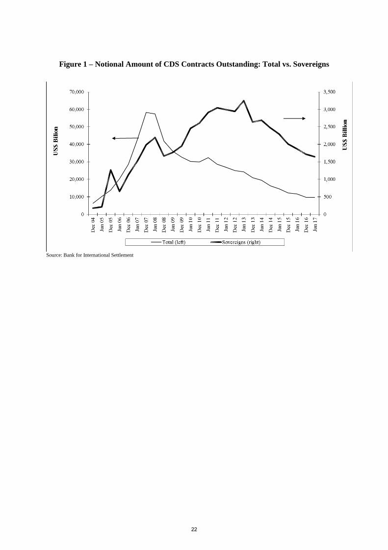
Figure 1 – Notional Amount of CDS Contracts Outstanding: Total vs. Sovereigns
Source: Bank for International Settlement
22
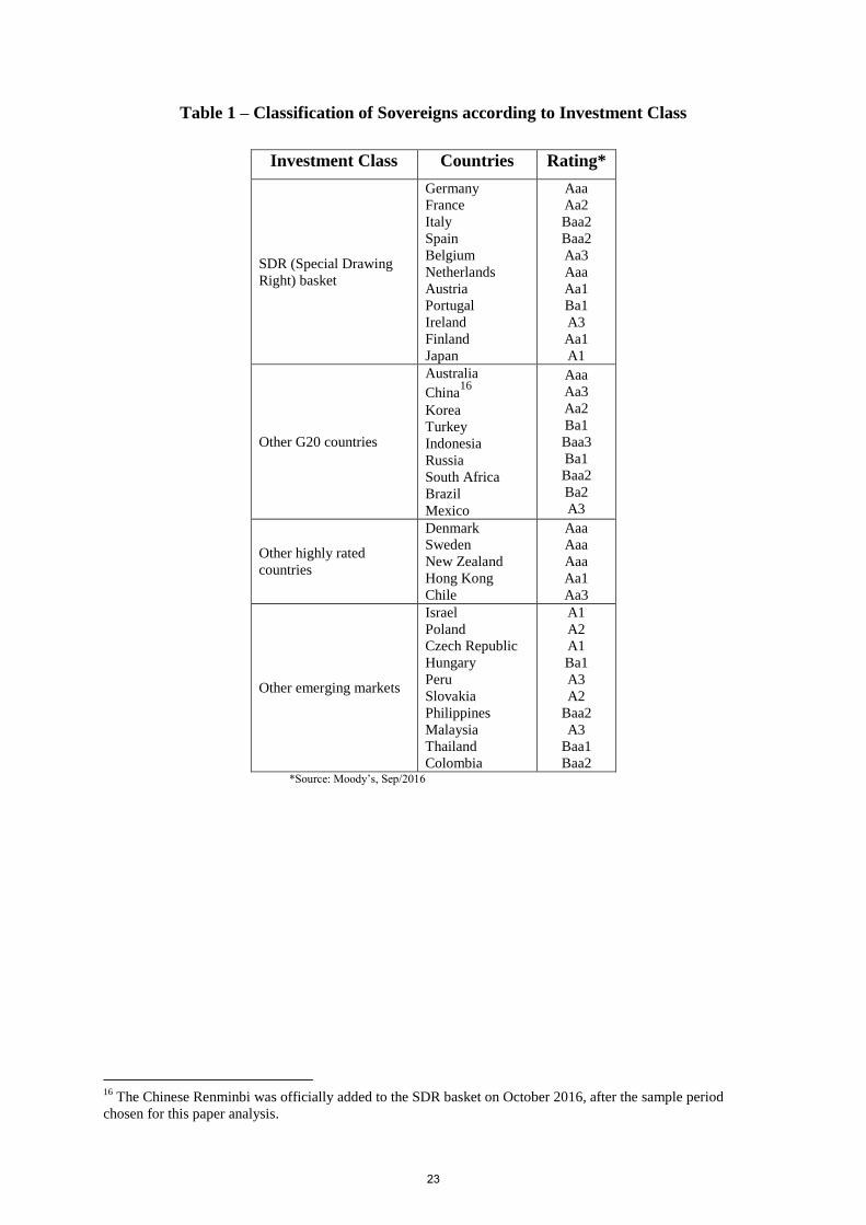
Table 1 – Classification of Sovereigns according to Investment Class
Investment Class Countries Rating*
SDR (Special Drawing
Right) basket
Germany
France
Italy
Spain
Belgium
Netherlands
Austria
Portugal
Ireland
Finland
Japan
Aaa
Aa2
Baa2
Baa2
Aa3
Aaa
Aa1
Ba1
A3
Aa1
A1
Other G20 countries
Australia
China16
Korea
Turkey
Indonesia
Russia
South Africa
Brazil
Mexico
Aaa
Aa3
Aa2
Ba1
Baa3
Ba1
Baa2
Ba2
A3
Other highly rated
countries
Denmark
Sweden
New Zealand
Hong Kong
Chile
Aaa
Aaa
Aaa
Aa1
Aa3
Other emerging markets
Israel
Poland
Czech Republic
Hungary
Peru
Slovakia
Philippines
Malaysia
Thailand
Colombia
A1
A2
A1
Ba1
A3
A2
Baa2
A3
Baa1
Baa2 *Source: Moody’s, Sep/2016
16
The Chinese Renminbi was officially added to the SDR basket on October 2016, after the sample period
chosen for this paper analysis.
23
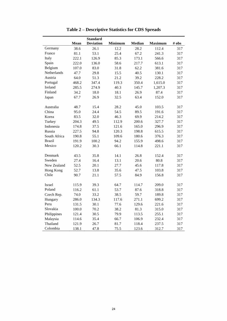
Table 2 – Descriptive Statistics for CDS Spreads
Mean
Standard
Deviation Minimum Median Maximum # obs
Germany 38.6 26.1 12.2 28.2 112.4 317
France 81.1 53.1 25.4 67.2 241.3 317
Italy 222.1 126.9 85.3 173.1 566.6 317
Spain 222.0 136.0 58.6 217.7 613.1 317
Belgium 107.0 83.0 31.8 62.2 381.6 317
Netherlands 47.7 29.8 15.5 40.5 130.1 317
Austria 64.0 51.3 21.2 39.2 228.2 317
Portugal 468.2 347.4 119.3 350.4 1,615.0 317
Ireland 285.5 274.9 40.3 145.7 1,207.3 317
Finland 34.2 18.0 18.1 26.9 87.4 317
Japan 67.7 26.9 32.5 63.4 152.0 317
Australia 48.7 15.4 28.2 45.0 103.5 317
China 95.0 24.4 54.5 89.5 191.6 317
Korea 83.5 32.0 46.3 69.9 214.2 317
Turkey 204.3 49.5 112.9 200.6 327.7 317
Indonesia 174.8 37.5 121.6 165.0 296.9 317
Russia 227.5 94.8 120.3 198.8 615.5 317
South Africa 190.8 55.1 109.6 180.6 376.3 317
Brazil 191.9 100.2 94.2 155.9 498.6 317
Mexico 120.2 30.3 66.1 114.8 221.1 317
Denmark 43.5 35.8 14.1 26.8 152.4 317
Sweden 27.4 16.4 13.1 20.6 80.8 317
New Zealand 52.5 20.1 27.7 45.6 117.8 317
Hong Kong 52.7 13.8 35.6 47.5 103.8 317
Chile 90.7 21.1 57.5 84.9 156.8 317
Israel 115.9 39.3 64.7 114.7 209.0 317
Poland 116.2 61.1 53.7 87.6 318.8 317
Czech Rep. 74.0 33.2 38.5 59.7 189.8 317
Hungary 286.0 134.3 117.6 271.1 699.2 317
Peru 131.5 30.1 77.6 129.6 221.6 317
Slovakia 100.0 70.2 38.2 81.3 315.0 317
Philippines 121.4 30.5 79.9 113.5 255.1 317
Malaysia 114.6 35.4 66.7 106.9 232.4 317
Thailand 121.9 26.7 81.7 118.4 237.5 317
Colombia 138.1 47.8 75.5 123.6 312.7 317
24
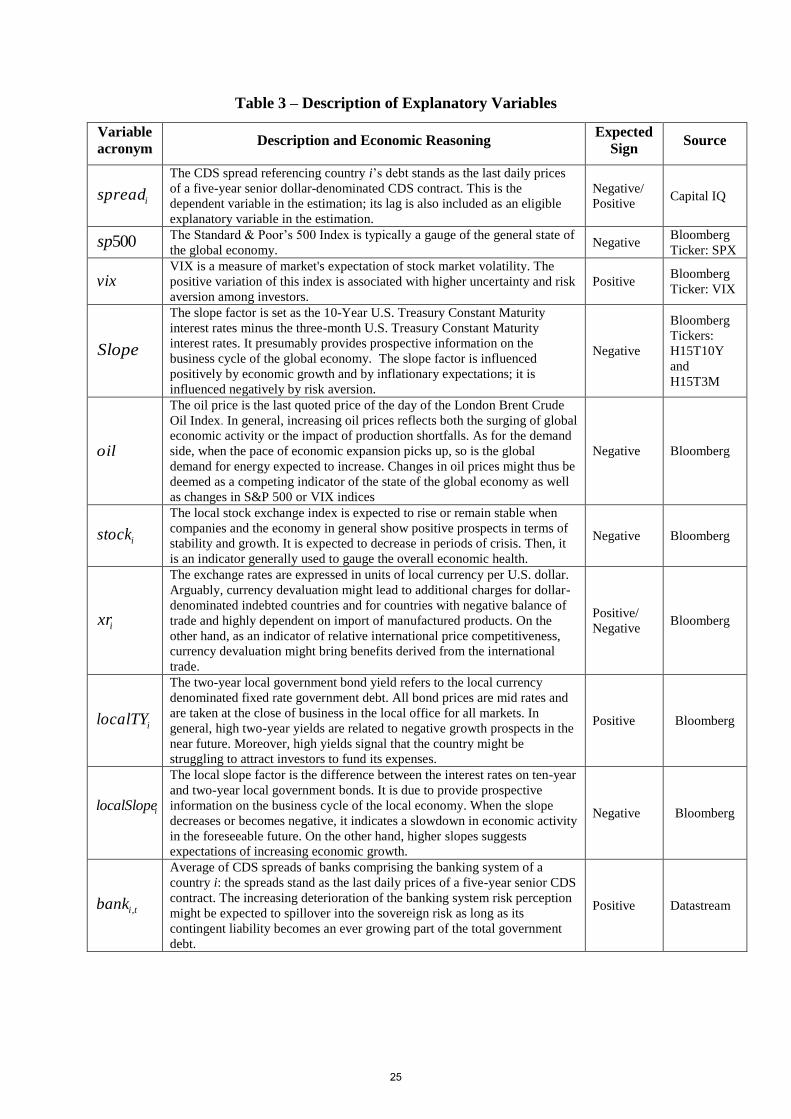
Table 3 – Description of Explanatory Variables
Variable
acronym Description and Economic Reasoning
Expected
Sign Source
ispread
The CDS spread referencing country i’s debt stands as the last daily prices
of a five-year senior dollar-denominated CDS contract. This is the
dependent variable in the estimation; its lag is also included as an eligible
explanatory variable in the estimation.
Negative/
Positive Capital IQ
500sp
The Standard & Poor’s 500 Index is typically a gauge of the general state of
the global economy. Negative
Bloomberg
Ticker: SPX
vix
VIX is a measure of market's expectation of stock market volatility. The
positive variation of this index is associated with higher uncertainty and risk
aversion among investors.
Positive Bloomberg
Ticker: VIX
Slope
The slope factor is set as the 10-Year U.S. Treasury Constant Maturity
interest rates minus the three-month U.S. Treasury Constant Maturity
interest rates. It presumably provides prospective information on the
business cycle of the global economy. The slope factor is influenced
positively by economic growth and by inflationary expectations; it is
influenced negatively by risk aversion.
Negative
Bloomberg
Tickers:
H15T10Y
and
H15T3M
oil
The oil price is the last quoted price of the day of the London Brent Crude
Oil Index. In general, increasing oil prices reflects both the surging of global
economic activity or the impact of production shortfalls. As for the demand
side, when the pace of economic expansion picks up, so is the global
demand for energy expected to increase. Changes in oil prices might thus be
deemed as a competing indicator of the state of the global economy as well
as changes in S&P 500 or VIX indices
Negative Bloomberg
istock
The local stock exchange index is expected to rise or remain stable when
companies and the economy in general show positive prospects in terms of
stability and growth. It is expected to decrease in periods of crisis. Then, it
is an indicator generally used to gauge the overall economic health.
Negative Bloomberg
ixr
The exchange rates are expressed in units of local currency per U.S. dollar.
Arguably, currency devaluation might lead to additional charges for dollar-
denominated indebted countries and for countries with negative balance of
trade and highly dependent on import of manufactured products. On the
other hand, as an indicator of relative international price competitiveness,
currency devaluation might bring benefits derived from the international
trade.
Positive/
Negative Bloomberg
ilocalTY
The two-year local government bond yield refers to the local currency
denominated fixed rate government debt. All bond prices are mid rates and
are taken at the close of business in the local office for all markets. In
general, high two-year yields are related to negative growth prospects in the
near future. Moreover, high yields signal that the country might be
struggling to attract investors to fund its expenses.
Positive Bloomberg
ilocalSlope
The local slope factor is the difference between the interest rates on ten-year
and two-year local government bonds. It is due to provide prospective
information on the business cycle of the local economy. When the slope
decreases or becomes negative, it indicates a slowdown in economic activity
in the foreseeable future. On the other hand, higher slopes suggests
expectations of increasing economic growth.
Negative Bloomberg
tibank ,
Average of CDS spreads of banks comprising the banking system of a
country i: the spreads stand as the last daily prices of a five-year senior CDS
contract. The increasing deterioration of the banking system risk perception
might be expected to spillover into the sovereign risk as long as its
contingent liability becomes an ever growing part of the total government
debt.
Positive Datastream
25
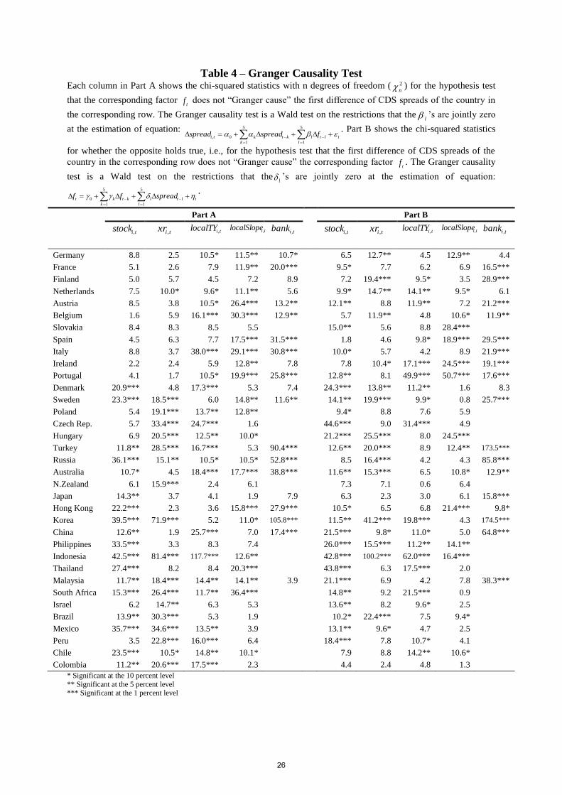
Table 4 – Granger Causality Test Each column in Part A shows the chi-squared statistics with n degrees of freedom ( 2
n ) for the hypothesis test
that the corresponding factor tf does not “Granger cause” the first difference of CDS spreads of the country in
the corresponding row. The Granger causality test is a Wald test on the restrictions that thel ’s are jointly zero
at the estimation of equation: t
l
ltl
k
ktkti fspreadspread
5
1
5
1
0,
. Part B shows the chi-squared statistics
for whether the opposite holds true, i.e., for the hypothesis test that the first difference of CDS spreads of the
country in the corresponding row does not “Granger cause” the corresponding factor tf . The Granger causality
test is a Wald test on the restrictions that thel ’s are jointly zero at the estimation of equation:
t
l
ltl
k
ktkt spreadff
5
1
5
1
0
.
Part A Part B
tistock ,
tixr ,
tilocalTY ,
tilocalSlope,
tibank , tistock ,
tixr ,
tilocalTY ,
tilocalSlope,
tibank ,
Germany 8.8 2.5 10.5* 11.5** 10.7* 6.5 12.7** 4.5 12.9** 4.4
France 5.1 2.6 7.9 11.9** 20.0*** 9.5* 7.7 6.2 6.9 16.5***
Finland 5.0 5.7 4.5 7.2 8.9 7.2 19.4*** 9.5* 3.5 28.9***
Netherlands 7.5 10.0* 9.6* 11.1** 5.6 9.9* 14.7** 14.1** 9.5* 6.1
Austria 8.5 3.8 10.5* 26.4*** 13.2** 12.1** 8.8 11.9** 7.2 21.2***
Belgium 1.6 5.9 16.1*** 30.3*** 12.9** 5.7 11.9** 4.8 10.6* 11.9**
Slovakia 8.4 8.3 8.5 5.5 15.0** 5.6 8.8 28.4***
Spain 4.5 6.3 7.7 17.5*** 31.5*** 1.8 4.6 9.8* 18.9*** 29.5***
Italy 8.8 3.7 38.0*** 29.1*** 30.8*** 10.0* 5.7 4.2 8.9 21.9***
Ireland 2.2 2.4 5.9 12.8** 7.8 7.8 10.4* 17.1*** 24.5*** 19.1***
Portugal 4.1 1.7 10.5* 19.9*** 25.8*** 12.8** 8.1 49.9*** 50.7*** 17.6***
Denmark 20.9*** 4.8 17.3*** 5.3 7.4 24.3*** 13.8** 11.2** 1.6 8.3
Sweden 23.3*** 18.5*** 6.0 14.8** 11.6** 14.1** 19.9*** 9.9* 0.8 25.7***
Poland 5.4 19.1*** 13.7** 12.8** 9.4* 8.8 7.6 5.9
Czech Rep. 5.7 33.4*** 24.7*** 1.6 44.6*** 9.0 31.4*** 4.9
Hungary 6.9 20.5*** 12.5** 10.0* 21.2*** 25.5*** 8.0 24.5***
Turkey 11.8** 28.5*** 16.7*** 5.3 90.4*** 12.6** 20.0*** 8.9 12.4** 173.5***
Russia 36.1*** 15.1** 10.5* 10.5* 52.8*** 8.5 16.4*** 4.2 4.3 85.8***
Australia 10.7* 4.5 18.4*** 17.7*** 38.8*** 11.6** 15.3*** 6.5 10.8* 12.9**
N.Zealand 6.1 15.9*** 2.4 6.1 7.3 7.1 0.6 6.4
Japan 14.3** 3.7 4.1 1.9 7.9 6.3 2.3 3.0 6.1 15.8***
Hong Kong 22.2*** 2.3 3.6 15.8*** 27.9*** 10.5* 6.5 6.8 21.4*** 9.8*
Korea 39.5*** 71.9*** 5.2 11.0* 105.8*** 11.5** 41.2*** 19.8*** 4.3 174.5***
China 12.6** 1.9 25.7*** 7.0 17.4*** 21.5*** 9.8* 11.0* 5.0 64.8***
Philippines 33.5*** 3.3 8.3 7.4 26.0*** 15.5*** 11.2** 14.1**
Indonesia 42.5*** 81.4*** 117.7*** 12.6** 42.8*** 100.2*** 62.0*** 16.4***
Thailand 27.4*** 8.2 8.4 20.3*** 43.8*** 6.3 17.5*** 2.0
Malaysia 11.7** 18.4*** 14.4** 14.1** 3.9 21.1*** 6.9 4.2 7.8 38.3***
South Africa 15.3*** 26.4*** 11.7** 36.4*** 14.8** 9.2 21.5*** 0.9
Israel 6.2 14.7** 6.3 5.3 13.6** 8.2 9.6* 2.5
Brazil 13.9** 30.3*** 5.3 1.9 10.2* 22.4*** 7.5 9.4*
Mexico 35.7*** 34.6*** 13.5** 3.9 13.1** 9.6* 4.7 2.5
Peru 3.5 22.8*** 16.0*** 6.4 18.4*** 7.8 10.7* 4.1
Chile 23.5*** 10.5* 14.8** 10.1* 7.9 8.8 14.2** 10.6*
Colombia 11.2** 20.6*** 17.5*** 2.3 4.4 2.4 4.8 1.3
* Significant at the 10 percent level
** Significant at the 5 percent level *** Significant at the 1 percent level
26
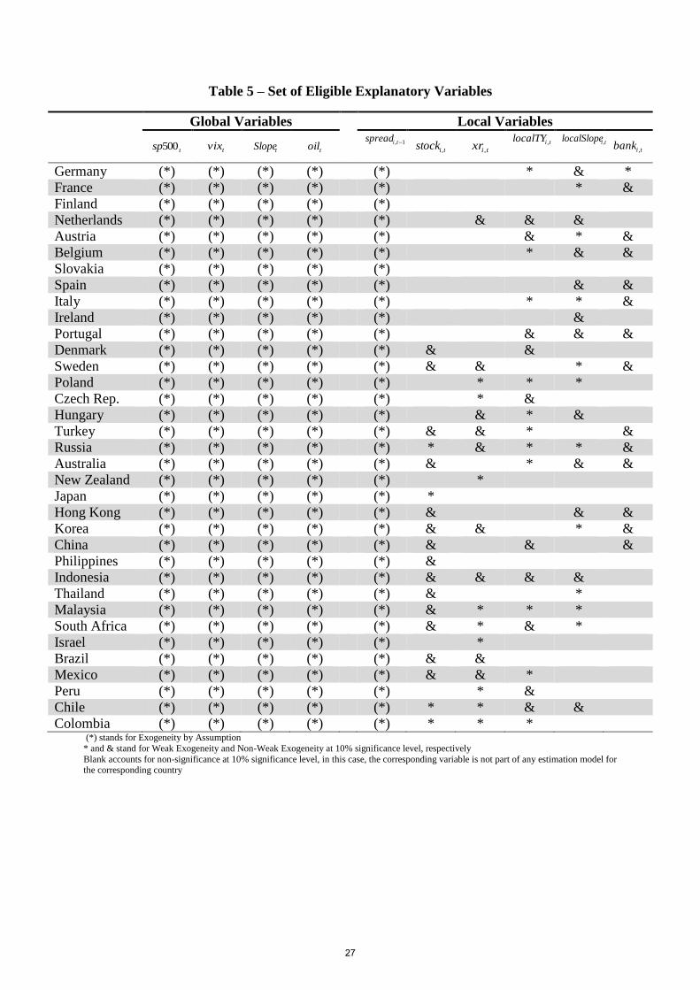
Table 5 – Set of Eligible Explanatory Variables
Global Variables Local Variables
tsp500 tvix
tSlope toil
1, tispread
tistock ,
tixr , tilocalTY ,
tilocalSlope,
tibank ,
Germany (*) (*) (*) (*) (*) * & *
France (*) (*) (*) (*) (*) * &
Finland (*) (*) (*) (*) (*)
Netherlands (*) (*) (*) (*) (*) & & &
Austria (*) (*) (*) (*) (*) & * &
Belgium (*) (*) (*) (*) (*) * & &
Slovakia (*) (*) (*) (*) (*)
Spain (*) (*) (*) (*) (*) & &
Italy (*) (*) (*) (*) (*) * * &
Ireland (*) (*) (*) (*) (*) &
Portugal (*) (*) (*) (*) (*) & & &
Denmark (*) (*) (*) (*) (*) & &
Sweden (*) (*) (*) (*) (*) & & * &
Poland (*) (*) (*) (*) (*) * * *
Czech Rep. (*) (*) (*) (*) (*) * &
Hungary (*) (*) (*) (*) (*) & * &
Turkey (*) (*) (*) (*) (*) & & * &
Russia (*) (*) (*) (*) (*) * & * * &
Australia (*) (*) (*) (*) (*) & * & &
New Zealand (*) (*) (*) (*) (*) *
Japan (*) (*) (*) (*) (*) *
Hong Kong (*) (*) (*) (*) (*) & & &
Korea (*) (*) (*) (*) (*) & & * &
China (*) (*) (*) (*) (*) & & &
Philippines (*) (*) (*) (*) (*) &
Indonesia (*) (*) (*) (*) (*) & & & &
Thailand (*) (*) (*) (*) (*) & *
Malaysia (*) (*) (*) (*) (*) & * * *
South Africa (*) (*) (*) (*) (*) & * & *
Israel (*) (*) (*) (*) (*) *
Brazil (*) (*) (*) (*) (*) & &
Mexico (*) (*) (*) (*) (*) & & *
Peru (*) (*) (*) (*) (*) * &
Chile (*) (*) (*) (*) (*) * * & &
Colombia (*) (*) (*) (*) (*) * * * (*) stands for Exogeneity by Assumption
* and & stand for Weak Exogeneity and Non-Weak Exogeneity at 10% significance level, respectively
Blank accounts for non-significance at 10% significance level, in this case, the corresponding variable is not part of any estimation model for the corresponding country
27
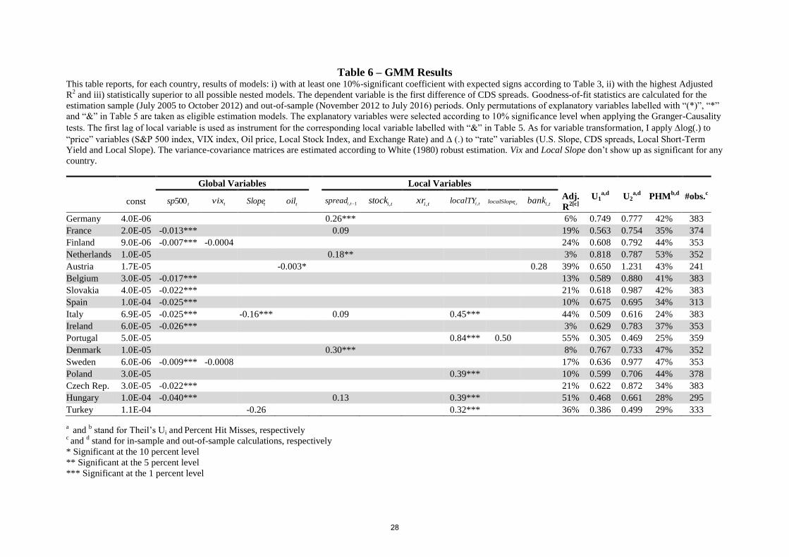
Table 6 – GMM Results This table reports, for each country, results of models: i) with at least one 10%-significant coefficient with expected signs according to Table 3, ii) with the highest Adjusted
R2 and iii) statistically superior to all possible nested models. The dependent variable is the first difference of CDS spreads. Goodness-of-fit statistics are calculated for the
estimation sample (July 2005 to October 2012) and out-of-sample (November 2012 to July 2016) periods. Only permutations of explanatory variables labelled with “(*)”, “*”
and “&” in Table 5 are taken as eligible estimation models. The explanatory variables were selected according to 10% significance level when applying the Granger-Causality
tests. The first lag of local variable is used as instrument for the corresponding local variable labelled with “&” in Table 5. As for variable transformation, I apply log(.) to
“price” variables (S&P 500 index, VIX index, Oil price, Local Stock Index, and Exchange Rate) and (.) to “rate” variables (U.S. Slope, CDS spreads, Local Short-Term
Yield and Local Slope). The variance-covariance matrices are estimated according to White (1980) robust estimation. Vix and Local Slope don’t show up as significant for any
country.
Global Variables Local Variables
const tsp500 tvix
tSlope toil 1, tispread
tistock ,
tixr ,
tilocalTY ,
tilocalSlope,
tibank , Adj.
R2[c]
U1a,d
U2a,d
PHMb,d
#obs.c
Germany 4.0E-06 0.26*** 6% 0.749 0.777 42% 383
France 2.0E-05 -0.013*** 0.09 19% 0.563 0.754 35% 374
Finland 9.0E-06 -0.007*** -0.0004 24% 0.608 0.792 44% 353
Netherlands 1.0E-05 0.18** 3% 0.818 0.787 53% 352
Austria 1.7E-05 -0.003* 0.28 39% 0.650 1.231 43% 241
Belgium 3.0E-05 -0.017*** 13% 0.589 0.880 41% 383
Slovakia 4.0E-05 -0.022*** 21% 0.618 0.987 42% 383
Spain 1.0E-04 -0.025*** 10% 0.675 0.695 34% 313
Italy 6.9E-05 -0.025*** -0.16*** 0.09 0.45*** 44% 0.509 0.616 24% 383
Ireland 6.0E-05 -0.026*** 3% 0.629 0.783 37% 353
Portugal 5.0E-05 0.84*** 0.50 55% 0.305 0.469 25% 359
Denmark 1.0E-05 0.30*** 8% 0.767 0.733 47% 352
Sweden 6.0E-06 -0.009*** -0.0008 17% 0.636 0.977 47% 353
Poland 3.0E-05 0.39*** 10% 0.599 0.706 44% 378
Czech Rep. 3.0E-05 -0.022*** 21% 0.622 0.872 34% 383
Hungary 1.0E-04 -0.040*** 0.13 0.39*** 51% 0.468 0.661 28% 295
Turkey 1.1E-04 -0.26 0.32*** 36% 0.386 0.499 29% 333
a and
b stand for Theil’s Ui and
Percent Hit Misses, respectively
c and
d stand for in-sample and out-of-sample calculations, respectively
* Significant at the 10 percent level
** Significant at the 5 percent level
*** Significant at the 1 percent level
28
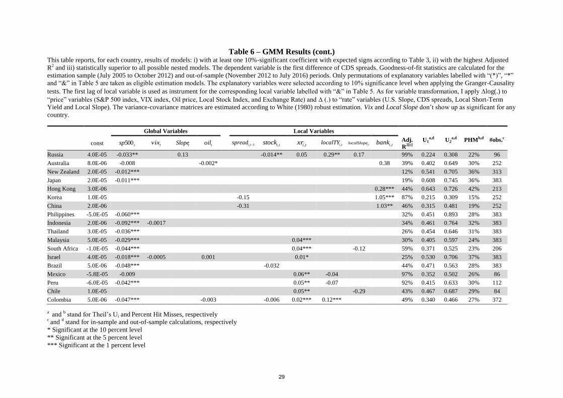
Table 6 – GMM Results (cont.) This table reports, for each country, results of models: i) with at least one 10%-significant coefficient with expected signs according to Table 3, ii) with the highest Adjusted
R2 and iii) statistically superior to all possible nested models. The dependent variable is the first difference of CDS spreads. Goodness-of-fit statistics are calculated for the
estimation sample (July 2005 to October 2012) and out-of-sample (November 2012 to July 2016) periods. Only permutations of explanatory variables labelled with “(*)”, “*”
and “&” in Table 5 are taken as eligible estimation models. The explanatory variables were selected according to 10% significance level when applying the Granger-Causality
tests. The first lag of local variable is used as instrument for the corresponding local variable labelled with “&” in Table 5. As for variable transformation, I apply log(.) to
“price” variables (S&P 500 index, VIX index, Oil price, Local Stock Index, and Exchange Rate) and (.) to “rate” variables (U.S. Slope, CDS spreads, Local Short-Term
Yield and Local Slope). The variance-covariance matrices are estimated according to White (1980) robust estimation. Vix and Local Slope don’t show up as significant for any
country.
Global Variables Local Variables
const tsp500 tvix
tSlope toil 1, tispread
tistock ,
tixr ,
tilocalTY ,
tilocalSlope,
tibank , Adj.
R2[c] U1
a,d U2a,d PHMb,d #obs.c
Russia 4.0E-05 -0.033** 0.13 -0.014** 0.05 0.29** 0.17 99% 0.224 0.308 22% 96
Australia 8.0E-06 -0.008 -0.002* 0.38 39% 0.402 0.649 30% 252
New Zealand 2.0E-05 -0.012*** 12% 0.541 0.705 36% 313
Japan 2.0E-05 -0.011*** 19% 0.608 0.745 36% 383
Hong Kong 3.0E-06 0.28*** 44% 0.643 0.726 42% 213
Korea 1.0E-05 -0.15 1.05*** 87% 0.215 0.309 15% 252
China 2.0E-06 -0.31 1.03** 46% 0.315 0.481 19% 252
Philippines -5.0E-05 -0.060*** 32% 0.451 0.893 28% 383
Indonesia 2.0E-06 -0.092*** -0.0017 34% 0.461 0.764 32% 383
Thailand 3.0E-05 -0.036*** 26% 0.454 0.646 31% 383
Malaysia 5.0E-05 -0.029*** 0.04*** 30% 0.405 0.597 24% 383
South Africa -1.0E-05 -0.044*** 0.04*** -0.12 59% 0.371 0.525 23% 206
Israel 4.0E-05 -0.018*** -0.0005 0.001 0.01* 25% 0.530 0.706 37% 383
Brazil 5.0E-06 -0.048*** -0.032 44% 0.471 0.563 28% 383
Mexico -5.8E-05 -0.009 0.06** -0.04 97% 0.352 0.502 26% 86
Peru -6.0E-05 -0.042*** 0.05** -0.07 92% 0.415 0.633 30% 112
Chile 1.0E-05 0.05** -0.29 43% 0.467 0.687 29% 84
Colombia 5.0E-06 -0.047*** -0.003 -0.006 0.02*** 0.12*** 49% 0.340 0.466 27% 372
a and
b stand for Theil’s Ui and
Percent Hit Misses, respectively
c and
d stand for in-sample and out-of-sample calculations, respectively
* Significant at the 10 percent level
** Significant at the 5 percent level
*** Significant at the 1 percent level
29

Table 7 – ARMA Results
When the goodness-of-fit statistics are better than those of Table 6, they are highlighted in bold.
AR Terms MA Terms
1 2
3 1 2
3 4
5 Adj. R2[c]
U1a,d U2
a,d PHM
b,d
Germany 0.3*** 6% 0.748 0.776 39%
France 0.1 1% 0.862 0.778 35%
Finland 0.4*** 10% 0.751 0.748 45%
Netherlands 0.2** 3% 0.807 0.781 44%
Austria 0.4*** 11% 0.710 0.780 38%
Belgium 0.2* 3% 0.817 0.755 40%
Slovakia 0.3*** 10% 0.767 0.760 51%
Spain 0.05 0% 0.948 0.744 39%
Italy 1.7*** -1.2*** 0.2* -1.7*** 1.0*** 8% 0.753 0.787 53%
Ireland 0.2*** -0.3 10% 0.733 0.798 50%
Portugal 1.0*** -0.8*** -0.4*** 0.1 -0.1 0.2*** 13% 0.691 0.929 39%
Denmark 0.3*** 9% 0.763 0.738 44%
Sweden 0.3*** 0.1 0.2 13% 0.765 0.768 46%
Poland 0.4*** 11% 0.767 0.765 42%
Czech Rep. 0.4*** 12% 0.804 0.746 56%
Hungary 0.3** -0.1 11% 0.735 0.763 44%
Turkey 0.2 -0.3 8% 0.765 0.732 44%
Russia 0.2 -0.4 0.1 0.3** 22% 0.698 0.804 45%
Australia 0.3*** 12% 0.732 0.788 42%
N.Zealand 0.3*** 9% 0.783 0.751 39%
Japan 0.1 0% 0.923 0.804 34%
Hong Kong 0.2* 4% 0.821 0.756 39%
Korea -0.6*** -0.2 0.8*** 11% 0.738 0.808 53%
China 0.3*** -0.3** 14% 0.724 0.822 49%
Philippines -0.5*** -0.3 0.6*** 11% 0.759 0.807 47%
Indonesia 0.3 -0.3* 16% 0.699 0.825 45%
Thailand -0.6*** -0.2 0.8*** 13% 0.741 0.838 48%
Malaysia -0.6*** -0.3 0.7*** 17% 0.711 0.812 45%
South Africa 0.2 -0.2 0.2* 11% 0.745 0.742 42%
Israel -0.4** 0.7*** 8% 0.756 0.776 42%
Brazil 0.2* -0.2 9% 0.749 0.729 39%
Mexico 0.3* -0.2 11% 0.741 0.737 47%
Peru -1.1*** -0.7*** 1.3*** 0.8*** 10% 0.737 0.745 43%
Chile -0.7*** 0.9*** 6% 0.775 0.744 39%
Colombia -1.1*** -0.7*** 1.4*** 0.8*** 9% 0.728 0.746 42%
The equation estimated by FIMLE is:
q
i
iti
p
i
itiit spreadspread11
,
a and
b stand for Theil’s Ui and
Percent Hit Misses, respectively;
c and
d stand for in-sample and out-of-sample
calculations, respectively
***, ** and * stand for significance at the 1%, 5% and 10% level, respectively.
30
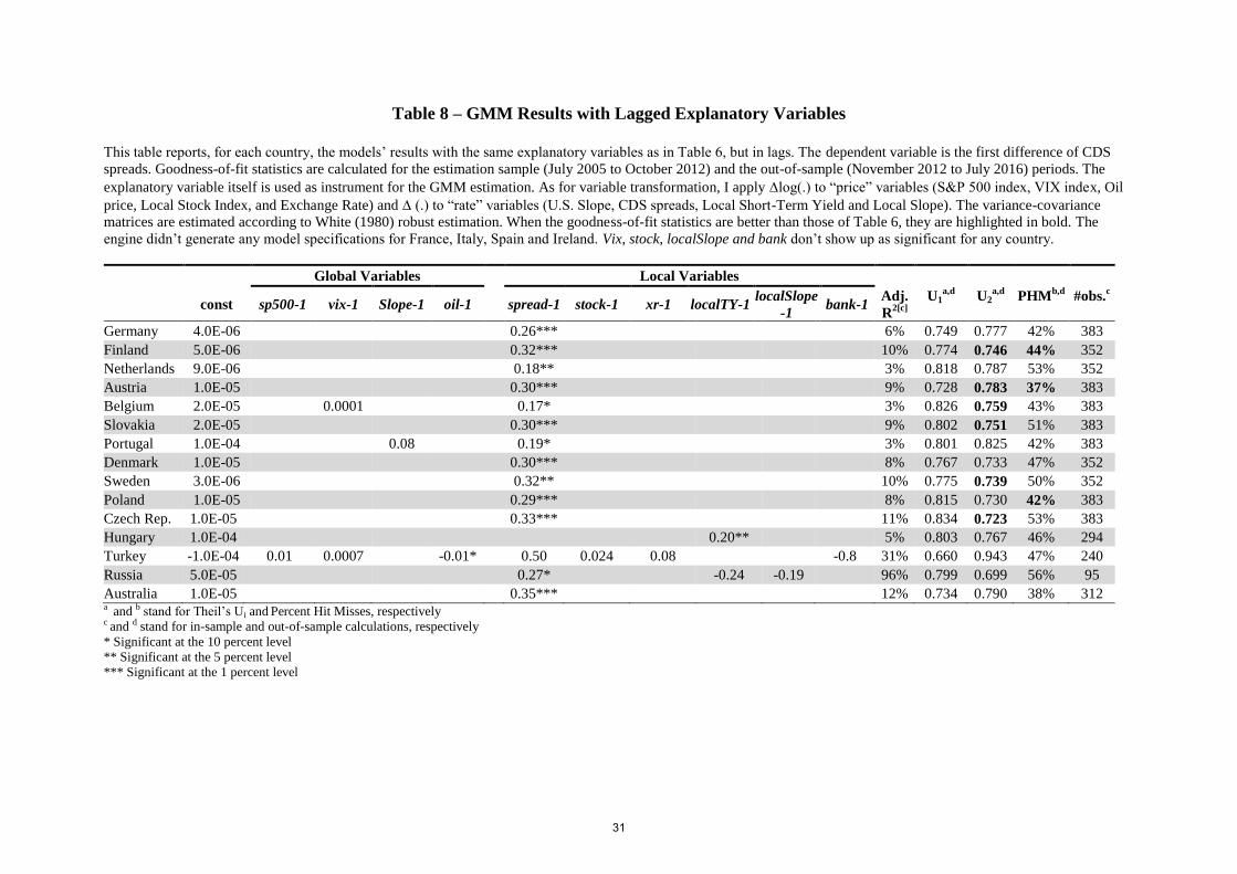
Table 8 – GMM Results with Lagged Explanatory Variables
This table reports, for each country, the models’ results with the same explanatory variables as in Table 6, but in lags. The dependent variable is the first difference of CDS
spreads. Goodness-of-fit statistics are calculated for the estimation sample (July 2005 to October 2012) and the out-of-sample (November 2012 to July 2016) periods. The
explanatory variable itself is used as instrument for the GMM estimation. As for variable transformation, I apply log(.) to “price” variables (S&P 500 index, VIX index, Oil
price, Local Stock Index, and Exchange Rate) and (.) to “rate” variables (U.S. Slope, CDS spreads, Local Short-Term Yield and Local Slope). The variance-covariance
matrices are estimated according to White (1980) robust estimation. When the goodness-of-fit statistics are better than those of Table 6, they are highlighted in bold. The
engine didn’t generate any model specifications for France, Italy, Spain and Ireland. Vix, stock, localSlope and bank don’t show up as significant for any country.
Global Variables Local Variables
const sp500-1 vix-1 Slope-1 oil-1 spread-1 stock-1 xr-1 localTY-1 localSlope
-1 bank-1
Adj.
R2[c]
U1a,d
U2a,d
PHMb,d
#obs.c
Germany 4.0E-06 0.26*** 6% 0.749 0.777 42% 383
Finland 5.0E-06 0.32*** 10% 0.774 0.746 44% 352
Netherlands 9.0E-06 0.18** 3% 0.818 0.787 53% 352
Austria 1.0E-05 0.30*** 9% 0.728 0.783 37% 383
Belgium 2.0E-05 0.0001 0.17* 3% 0.826 0.759 43% 383
Slovakia 2.0E-05 0.30*** 9% 0.802 0.751 51% 383
Portugal 1.0E-04 0.08 0.19* 3% 0.801 0.825 42% 383
Denmark 1.0E-05 0.30*** 8% 0.767 0.733 47% 352
Sweden 3.0E-06 0.32** 10% 0.775 0.739 50% 352
Poland 1.0E-05 0.29*** 8% 0.815 0.730 42% 383
Czech Rep. 1.0E-05 0.33*** 11% 0.834 0.723 53% 383
Hungary 1.0E-04 0.20** 5% 0.803 0.767 46% 294
Turkey -1.0E-04 0.01 0.0007 -0.01* 0.50 0.024 0.08 -0.8 31% 0.660 0.943 47% 240
Russia 5.0E-05 0.27* -0.24 -0.19 96% 0.799 0.699 56% 95
Australia 1.0E-05 0.35*** 12% 0.734 0.790 38% 312 a and b stand for Theil’s Ui and Percent Hit Misses, respectively c and d stand for in-sample and out-of-sample calculations, respectively
* Significant at the 10 percent level
** Significant at the 5 percent level
*** Significant at the 1 percent level
31
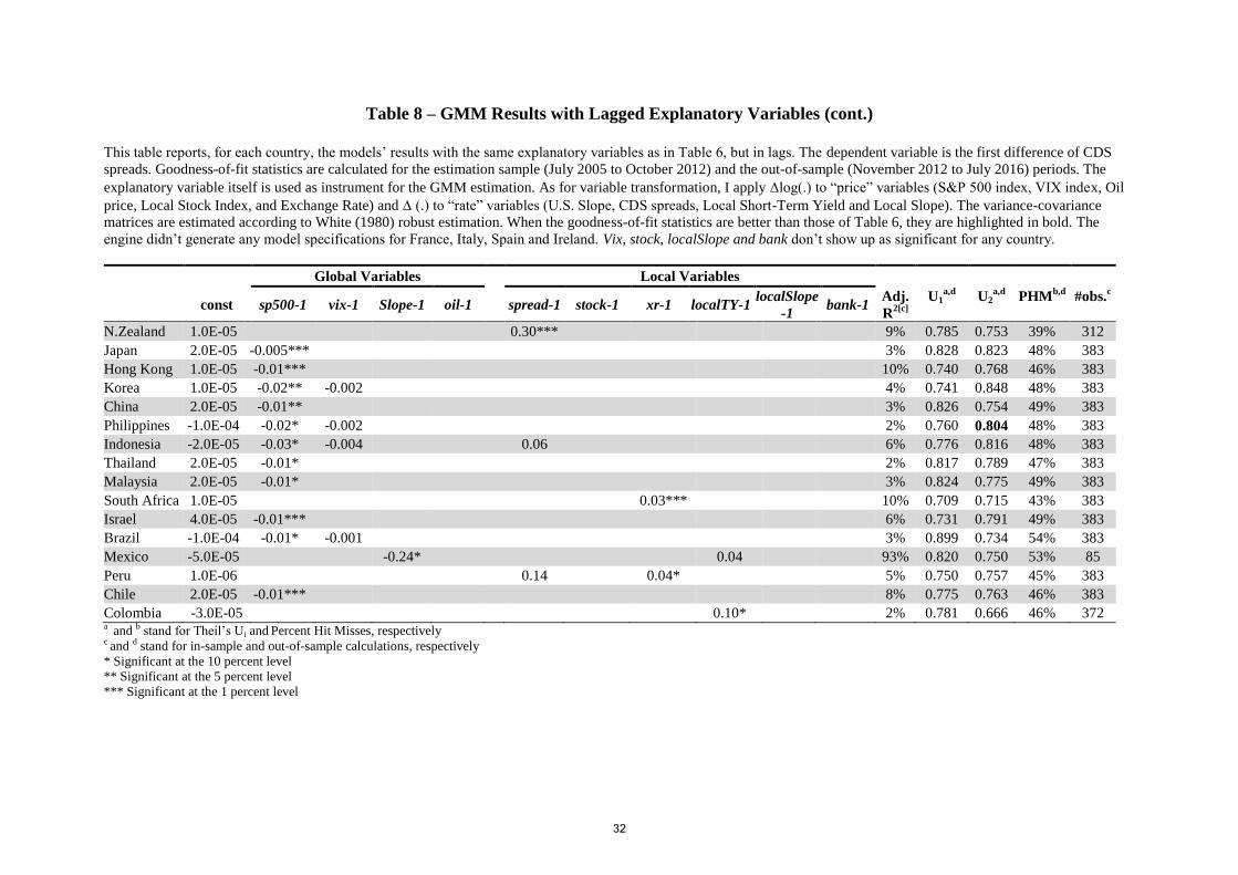
Table 8 – GMM Results with Lagged Explanatory Variables (cont.)
This table reports, for each country, the models’ results with the same explanatory variables as in Table 6, but in lags. The dependent variable is the first difference of CDS
spreads. Goodness-of-fit statistics are calculated for the estimation sample (July 2005 to October 2012) and the out-of-sample (November 2012 to July 2016) periods. The
explanatory variable itself is used as instrument for the GMM estimation. As for variable transformation, I apply log(.) to “price” variables (S&P 500 index, VIX index, Oil
price, Local Stock Index, and Exchange Rate) and (.) to “rate” variables (U.S. Slope, CDS spreads, Local Short-Term Yield and Local Slope). The variance-covariance
matrices are estimated according to White (1980) robust estimation. When the goodness-of-fit statistics are better than those of Table 6, they are highlighted in bold. The
engine didn’t generate any model specifications for France, Italy, Spain and Ireland. Vix, stock, localSlope and bank don’t show up as significant for any country.
Global Variables Local Variables
const sp500-1 vix-1 Slope-1 oil-1 spread-1 stock-1 xr-1 localTY-1 localSlope
-1 bank-1
Adj.
R2[c]
U1a,d
U2a,d
PHMb,d
#obs.c
N.Zealand 1.0E-05 0.30*** 9% 0.785 0.753 39% 312
Japan 2.0E-05 -0.005*** 3% 0.828 0.823 48% 383
Hong Kong 1.0E-05 -0.01*** 10% 0.740 0.768 46% 383
Korea 1.0E-05 -0.02** -0.002 4% 0.741 0.848 48% 383
China 2.0E-05 -0.01** 3% 0.826 0.754 49% 383
Philippines -1.0E-04 -0.02* -0.002 2% 0.760 0.804 48% 383
Indonesia -2.0E-05 -0.03* -0.004 0.06 6% 0.776 0.816 48% 383
Thailand 2.0E-05 -0.01* 2% 0.817 0.789 47% 383
Malaysia 2.0E-05 -0.01* 3% 0.824 0.775 49% 383
South Africa 1.0E-05 0.03*** 10% 0.709 0.715 43% 383
Israel 4.0E-05 -0.01*** 6% 0.731 0.791 49% 383
Brazil -1.0E-04 -0.01* -0.001 3% 0.899 0.734 54% 383
Mexico -5.0E-05 -0.24* 0.04 93% 0.820 0.750 53% 85
Peru 1.0E-06 0.14 0.04* 5% 0.750 0.757 45% 383
Chile 2.0E-05 -0.01*** 8% 0.775 0.763 46% 383
Colombia -3.0E-05 0.10* 2% 0.781 0.666 46% 372 a and b stand for Theil’s Ui and Percent Hit Misses, respectively c and d stand for in-sample and out-of-sample calculations, respectively
* Significant at the 10 percent level
** Significant at the 5 percent level
*** Significant at the 1 percent level
32
31/51
Table 9 – GMM Results
without the criterion “with at least one 10%-significant coefficient with expected signs according to Table 3” This table reports, for each country, results of models: i) with the highest Adjusted R
2 and ii) statistically superior to all possible nested models. The dependent variable is the
first difference of CDS spreads. Goodness-of-fit statistics are calculated for the estimation sample (July 2005 to October 2012) and out-of-sample (November 2012 to July
2016) periods. Only permutations of explanatory variables labelled with “(*)”, “*” and “&” in Table 5 are taken as eligible estimation models. The explanatory variables were
selected according to 10% significance level when applying the Granger-Causality tests. The first lag of local variable is used as instrument for the corresponding local
variable labelled with “&” in Table 5. As for variable transformation, I apply log(.) to “price” variables (S&P 500 index, VIX index, Oil price, Local Stock Index, and
Exchange Rate) and (.) to “rate” variables (U.S. Slope, CDS spreads, Local Short-Term Yield and Local Slope). The variance-covariance matrices are estimated according
to White (1980) robust estimation. When model specifications show up as different from Table 6, they are highlighted in bold. Oil doesn’t show up as significant for any
country. Vix and oil estimators aren’t significant for any model.
Global Variables Local Variables
const tsp500 tvix
tSlope toil 1, tispread
tistock ,
tixr ,
tilocalTY ,
tilocalSlope,
tibank , Adj.
R2[c] U1
a,d U2a,d PHMb,d #obs.c
Germany 4.0E-06 0.26*** 6% 0.749 0.777 42% 383
France 2.0E-05 -0.012 -0.07 0.03 0.09 37% 0.505 0.731 29% 252
Finland 9.0E-06 -0.007*** -0.0004 24% 0.608 0.792 44% 353
Netherlands 1.0E-05 0.18** 3% 0.818 0.787 53% 352
Austria 1.7E-05 -0.020*** -0.002* 24% 0.609 1.197 40% 383
Belgium 3.0E-05 -0.017*** 13% 0.589 0.880 41% 383
Slovakia 4.0E-05 -0.022*** 21% 0.618 0.987 42% 383
Spain 1.0E-04 -0.025*** 10% 0.675 0.695 34% 313
Italy 6.0E-05 -0.026*** -0.21*** 0.07 0.67*** 0.40** 48% 0.420 0.536 21% 383
Ireland 6.0E-05 -0.026*** 3% 0.629 0.783 37% 353
Portugal 5.0E-05 0.84*** 0.50 55% 0.305 0.469 25% 359
Denmark 1.0E-05 -0.010*** -0.001* 17% 0.648 0.979 47% 353
Sweden 6.0E-06 -0.009*** -0.0008 17% 0.636 0.977 47% 353
Poland 3.0E-05 0.39*** 10% 0.599 0.706 44% 378
Czech Rep. 3.0E-05 -0.022*** 21% 0.622 0.872 34% 383
Hungary 1.0E-04 -0.040*** 0.13 0.39*** 51% 0.468 0.661 28% 295
Turkey 1.1E-04 -0.26 0.32*** 36% 0.386 0.499 29% 333 a and
b stand for Theil’s Ui and
Percent Hit Misses, respectively
c and
d stand for in-sample and out-of-sample calculations, respectively
* Significant at the 10 percent level
** Significant at the 5 percent level
*** Significant at the 1 percent level
33
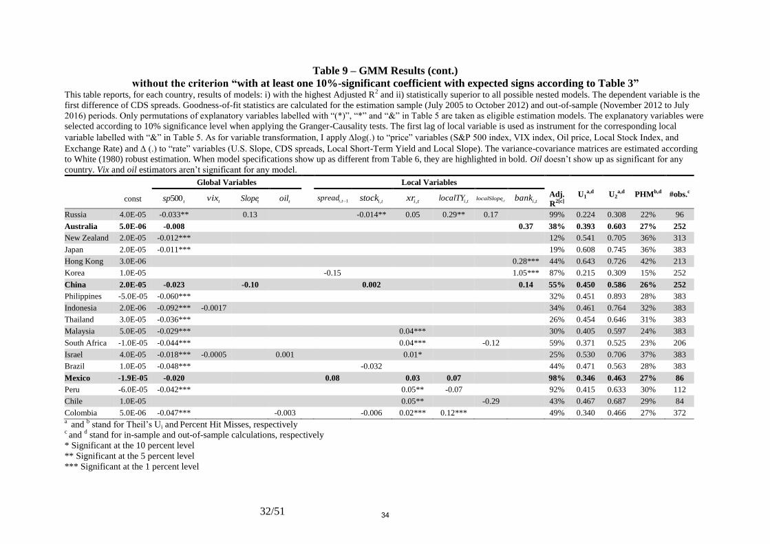
32/51
Table 9 – GMM Results (cont.)
without the criterion “with at least one 10%-significant coefficient with expected signs according to Table 3” This table reports, for each country, results of models: i) with the highest Adjusted R
2 and ii) statistically superior to all possible nested models. The dependent variable is the
first difference of CDS spreads. Goodness-of-fit statistics are calculated for the estimation sample (July 2005 to October 2012) and out-of-sample (November 2012 to July
2016) periods. Only permutations of explanatory variables labelled with “(*)”, “*” and “&” in Table 5 are taken as eligible estimation models. The explanatory variables were
selected according to 10% significance level when applying the Granger-Causality tests. The first lag of local variable is used as instrument for the corresponding local
variable labelled with “&” in Table 5. As for variable transformation, I apply log(.) to “price” variables (S&P 500 index, VIX index, Oil price, Local Stock Index, and
Exchange Rate) and (.) to “rate” variables (U.S. Slope, CDS spreads, Local Short-Term Yield and Local Slope). The variance-covariance matrices are estimated according
to White (1980) robust estimation. When model specifications show up as different from Table 6, they are highlighted in bold. Oil doesn’t show up as significant for any
country. Vix and oil estimators aren’t significant for any model.
Global Variables Local Variables
const tsp500 tvix
tSlope toil 1, tispread
tistock ,
tixr ,
tilocalTY ,
tilocalSlope,
tibank , Adj.
R2[c] U1
a,d U2a,d PHMb,d #obs.c
Russia 4.0E-05 -0.033** 0.13 -0.014** 0.05 0.29** 0.17 99% 0.224 0.308 22% 96
Australia 5.0E-06 -0.008 0.37 38% 0.393 0.603 27% 252
New Zealand 2.0E-05 -0.012*** 12% 0.541 0.705 36% 313
Japan 2.0E-05 -0.011*** 19% 0.608 0.745 36% 383
Hong Kong 3.0E-06 0.28*** 44% 0.643 0.726 42% 213
Korea 1.0E-05 -0.15 1.05*** 87% 0.215 0.309 15% 252
China 2.0E-05 -0.023 -0.10 0.002 0.14 55% 0.450 0.586 26% 252
Philippines -5.0E-05 -0.060*** 32% 0.451 0.893 28% 383
Indonesia 2.0E-06 -0.092*** -0.0017 34% 0.461 0.764 32% 383
Thailand 3.0E-05 -0.036*** 26% 0.454 0.646 31% 383
Malaysia 5.0E-05 -0.029*** 0.04*** 30% 0.405 0.597 24% 383
South Africa -1.0E-05 -0.044*** 0.04*** -0.12 59% 0.371 0.525 23% 206
Israel 4.0E-05 -0.018*** -0.0005 0.001 0.01* 25% 0.530 0.706 37% 383
Brazil 1.0E-05 -0.048*** -0.032 44% 0.471 0.563 28% 383
Mexico -1.9E-05 -0.020 0.08 0.03 0.07 98% 0.346 0.463 27% 86
Peru -6.0E-05 -0.042*** 0.05** -0.07 92% 0.415 0.633 30% 112
Chile 1.0E-05 0.05** -0.29 43% 0.467 0.687 29% 84
Colombia 5.0E-06 -0.047*** -0.003 -0.006 0.02*** 0.12*** 49% 0.340 0.466 27% 372 a and
b stand for Theil’s Ui and
Percent Hit Misses, respectively
c and
d stand for in-sample and out-of-sample calculations, respectively
* Significant at the 10 percent level
** Significant at the 5 percent level
*** Significant at the 1 percent level
34
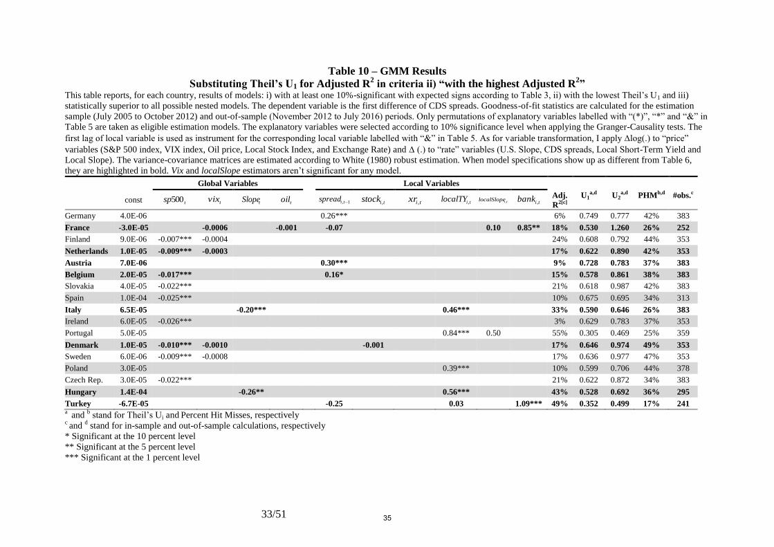
33/51
Table 10 – GMM Results
Substituting Theil’s U1 for Adjusted R2 in criteria ii) “with the highest Adjusted R
2”
This table reports, for each country, results of models: i) with at least one 10%-significant with expected signs according to Table 3, ii) with the lowest Theil’s U1 and iii)
statistically superior to all possible nested models. The dependent variable is the first difference of CDS spreads. Goodness-of-fit statistics are calculated for the estimation
sample (July 2005 to October 2012) and out-of-sample (November 2012 to July 2016) periods. Only permutations of explanatory variables labelled with “(*)”, “*” and “&” in
Table 5 are taken as eligible estimation models. The explanatory variables were selected according to 10% significance level when applying the Granger-Causality tests. The
first lag of local variable is used as instrument for the corresponding local variable labelled with “&” in Table 5. As for variable transformation, I apply log(.) to “price”
variables (S&P 500 index, VIX index, Oil price, Local Stock Index, and Exchange Rate) and (.) to “rate” variables (U.S. Slope, CDS spreads, Local Short-Term Yield and
Local Slope). The variance-covariance matrices are estimated according to White (1980) robust estimation. When model specifications show up as different from Table 6,
they are highlighted in bold. Vix and localSlope estimators aren’t significant for any model.
Global Variables Local Variables
const tsp500 tvix
tSlope toil 1, tispread
tistock ,
tixr ,
tilocalTY ,
tilocalSlope,
tibank , Adj.
R2[c] U1
a,d U2a,d PHMb,d #obs.c
Germany 4.0E-06 0.26*** 6% 0.749 0.777 42% 383
France -3.0E-05 -0.0006 -0.001 -0.07 0.10 0.85** 18% 0.530 1.260 26% 252
Finland 9.0E-06 -0.007*** -0.0004 24% 0.608 0.792 44% 353
Netherlands 1.0E-05 -0.009*** -0.0003 17% 0.622 0.890 42% 353
Austria 7.0E-06 0.30*** 9% 0.728 0.783 37% 383
Belgium 2.0E-05 -0.017*** 0.16* 15% 0.578 0.861 38% 383
Slovakia 4.0E-05 -0.022*** 21% 0.618 0.987 42% 383
Spain 1.0E-04 -0.025*** 10% 0.675 0.695 34% 313
Italy 6.5E-05 -0.20*** 0.46*** 33% 0.590 0.646 26% 383
Ireland 6.0E-05 -0.026*** 3% 0.629 0.783 37% 353
Portugal 5.0E-05 0.84*** 0.50 55% 0.305 0.469 25% 359
Denmark 1.0E-05 -0.010*** -0.0010 -0.001 17% 0.646 0.974 49% 353
Sweden 6.0E-06 -0.009*** -0.0008 17% 0.636 0.977 47% 353
Poland 3.0E-05 0.39*** 10% 0.599 0.706 44% 378
Czech Rep. 3.0E-05 -0.022*** 21% 0.622 0.872 34% 383
Hungary 1.4E-04 -0.26** 0.56*** 43% 0.528 0.692 36% 295
Turkey -6.7E-05 -0.25 0.03 1.09*** 49% 0.352 0.499 17% 241 a and
b stand for Theil’s Ui and
Percent Hit Misses, respectively
c and
d stand for in-sample and out-of-sample calculations, respectively
* Significant at the 10 percent level
** Significant at the 5 percent level
*** Significant at the 1 percent level
35
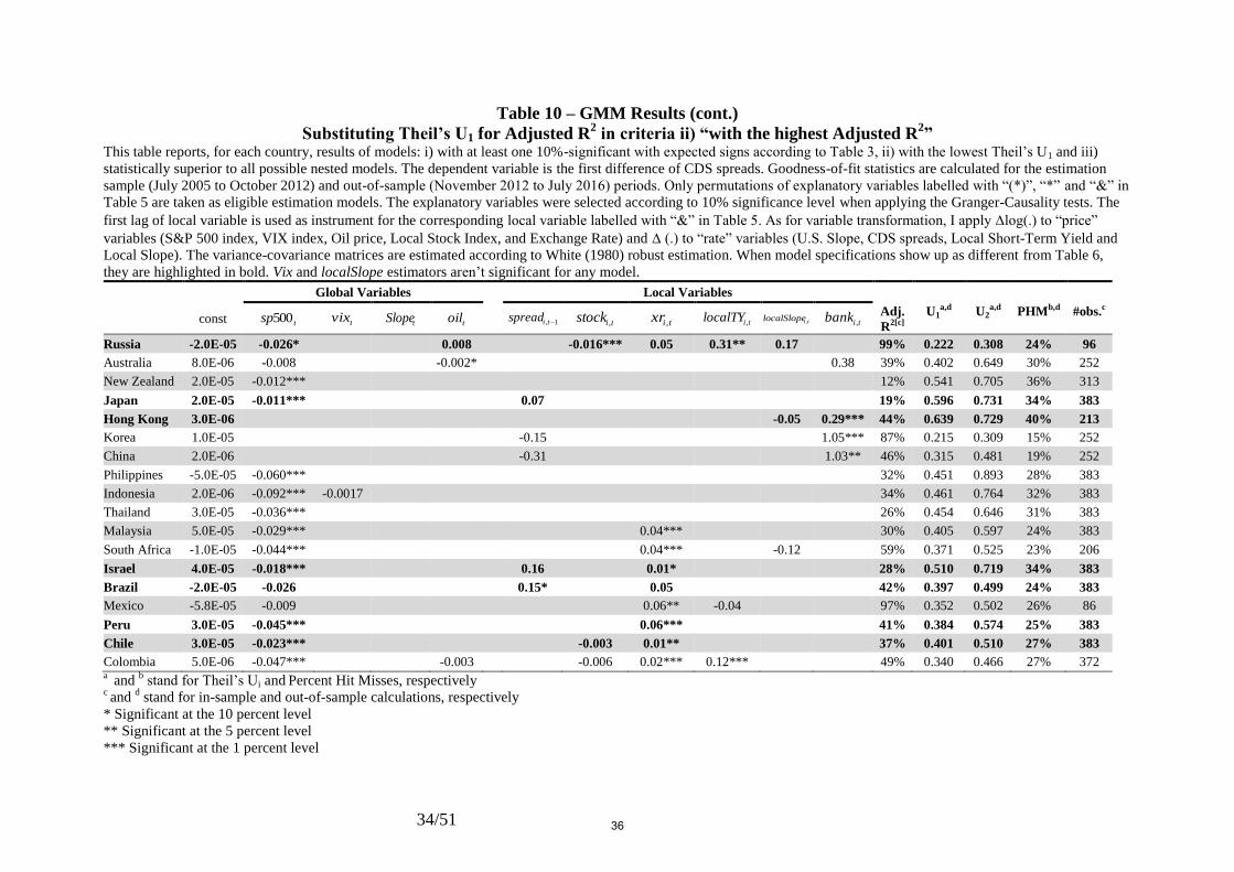
34/51
Table 10 – GMM Results (cont.)
Substituting Theil’s U1 for Adjusted R2 in criteria ii) “with the highest Adjusted R
2”
This table reports, for each country, results of models: i) with at least one 10%-significant with expected signs according to Table 3, ii) with the lowest Theil’s U1 and iii)
statistically superior to all possible nested models. The dependent variable is the first difference of CDS spreads. Goodness-of-fit statistics are calculated for the estimation
sample (July 2005 to October 2012) and out-of-sample (November 2012 to July 2016) periods. Only permutations of explanatory variables labelled with “(*)”, “*” and “&” in
Table 5 are taken as eligible estimation models. The explanatory variables were selected according to 10% significance level when applying the Granger-Causality tests. The
first lag of local variable is used as instrument for the corresponding local variable labelled with “&” in Table 5. As for variable transformation, I apply log(.) to “price”
variables (S&P 500 index, VIX index, Oil price, Local Stock Index, and Exchange Rate) and (.) to “rate” variables (U.S. Slope, CDS spreads, Local Short-Term Yield and
Local Slope). The variance-covariance matrices are estimated according to White (1980) robust estimation. When model specifications show up as different from Table 6,
they are highlighted in bold. Vix and localSlope estimators aren’t significant for any model.
Global Variables Local Variables
const tsp500 tvix
tSlope toil 1, tispread
tistock ,
tixr ,
tilocalTY ,
tilocalSlope,
tibank , Adj.
R2[c] U1
a,d U2a,d PHMb,d #obs.c
Russia -2.0E-05 -0.026* 0.008 -0.016*** 0.05 0.31** 0.17 99% 0.222 0.308 24% 96
Australia 8.0E-06 -0.008 -0.002* 0.38 39% 0.402 0.649 30% 252
New Zealand 2.0E-05 -0.012*** 12% 0.541 0.705 36% 313
Japan 2.0E-05 -0.011*** 0.07 19% 0.596 0.731 34% 383
Hong Kong 3.0E-06 -0.05 0.29*** 44% 0.639 0.729 40% 213
Korea 1.0E-05 -0.15 1.05*** 87% 0.215 0.309 15% 252
China 2.0E-06 -0.31 1.03** 46% 0.315 0.481 19% 252
Philippines -5.0E-05 -0.060*** 32% 0.451 0.893 28% 383
Indonesia 2.0E-06 -0.092*** -0.0017 34% 0.461 0.764 32% 383
Thailand 3.0E-05 -0.036*** 26% 0.454 0.646 31% 383
Malaysia 5.0E-05 -0.029*** 0.04*** 30% 0.405 0.597 24% 383
South Africa -1.0E-05 -0.044*** 0.04*** -0.12 59% 0.371 0.525 23% 206
Israel 4.0E-05 -0.018*** 0.16 0.01* 28% 0.510 0.719 34% 383
Brazil -2.0E-05 -0.026 0.15* 0.05 42% 0.397 0.499 24% 383
Mexico -5.8E-05 -0.009 0.06** -0.04 97% 0.352 0.502 26% 86
Peru 3.0E-05 -0.045*** 0.06*** 41% 0.384 0.574 25% 383
Chile 3.0E-05 -0.023*** -0.003 0.01** 37% 0.401 0.510 27% 383
Colombia 5.0E-06 -0.047*** -0.003 -0.006 0.02*** 0.12*** 49% 0.340 0.466 27% 372 a and
b stand for Theil’s Ui and
Percent Hit Misses, respectively
c and
d stand for in-sample and out-of-sample calculations, respectively
* Significant at the 10 percent level
** Significant at the 5 percent level
*** Significant at the 1 percent level
36
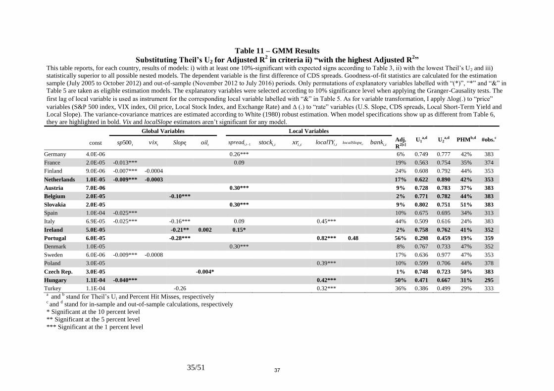
35/51
Table 11 – GMM Results
Substituting Theil’s U2 for Adjusted R2 in criteria ii) “with the highest Adjusted R
2”
This table reports, for each country, results of models: i) with at least one 10%-significant with expected signs according to Table 3, ii) with the lowest Theil’s U2 and iii)
statistically superior to all possible nested models. The dependent variable is the first difference of CDS spreads. Goodness-of-fit statistics are calculated for the estimation
sample (July 2005 to October 2012) and out-of-sample (November 2012 to July 2016) periods. Only permutations of explanatory variables labelled with “(*)”, “*” and “&” in
Table 5 are taken as eligible estimation models. The explanatory variables were selected according to 10% significance level when applying the Granger-Causality tests. The
first lag of local variable is used as instrument for the corresponding local variable labelled with “&” in Table 5. As for variable transformation, I apply log(.) to “price”
variables (S&P 500 index, VIX index, Oil price, Local Stock Index, and Exchange Rate) and (.) to “rate” variables (U.S. Slope, CDS spreads, Local Short-Term Yield and
Local Slope). The variance-covariance matrices are estimated according to White (1980) robust estimation. When model specifications show up as different from Table 6,
they are highlighted in bold. Vix and localSlope estimators aren’t significant for any model.
Global Variables Local Variables
const tsp500 tvix
tSlope toil 1, tispread
tistock ,
tixr ,
tilocalTY ,
tilocalSlope,
tibank , Adj.
R2[c] U1
a,d U2a,d PHMb,d #obs.c
Germany 4.0E-06 0.26*** 6% 0.749 0.777 42% 383
France 2.0E-05 -0.013*** 0.09 19% 0.563 0.754 35% 374
Finland 9.0E-06 -0.007*** -0.0004 24% 0.608 0.792 44% 353
Netherlands 1.0E-05 -0.009*** -0.0003 17% 0.622 0.890 42% 353
Austria 7.0E-06 0.30*** 9% 0.728 0.783 37% 383
Belgium 2.0E-05 -0.10*** 2% 0.771 0.782 44% 383
Slovakia 2.0E-05 0.30*** 9% 0.802 0.751 51% 383
Spain 1.0E-04 -0.025*** 10% 0.675 0.695 34% 313
Italy 6.9E-05 -0.025*** -0.16*** 0.09 0.45*** 44% 0.509 0.616 24% 383
Ireland 5.0E-05 -0.21** 0.002 0.15* 2% 0.758 0.762 41% 352
Portugal 6.0E-05 -0.28*** 0.82*** 0.48 56% 0.298 0.459 19% 359
Denmark 1.0E-05 0.30*** 8% 0.767 0.733 47% 352
Sweden 6.0E-06 -0.009*** -0.0008 17% 0.636 0.977 47% 353
Poland 3.0E-05 0.39*** 10% 0.599 0.706 44% 378
Czech Rep. 3.0E-05 -0.004* 1% 0.748 0.723 50% 383
Hungary 1.1E-04 -0.040*** 0.42*** 50% 0.471 0.667 31% 295
Turkey 1.1E-04 -0.26 0.32*** 36% 0.386 0.499 29% 333 a and
b stand for Theil’s Ui and
Percent Hit Misses, respectively
c and
d stand for in-sample and out-of-sample calculations, respectively
* Significant at the 10 percent level
** Significant at the 5 percent level
*** Significant at the 1 percent level
37
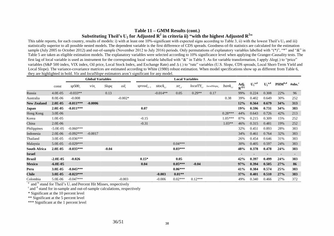
36/51
Table 11 – GMM Results (cont.)
Substituting Theil’s U2 for Adjusted R2 in criteria ii) “with the highest Adjusted R
2”
This table reports, for each country, results of models: i) with at least one 10%-significant with expected signs according to Table 3, ii) with the lowest Theil’s U2 and iii)
statistically superior to all possible nested models. The dependent variable is the first difference of CDS spreads. Goodness-of-fit statistics are calculated for the estimation
sample (July 2005 to October 2012) and out-of-sample (November 2012 to July 2016) periods. Only permutations of explanatory variables labelled with “(*)”, “*” and “&” in
Table 5 are taken as eligible estimation models. The explanatory variables were selected according to 10% significance level when applying the Granger-Causality tests. The
first lag of local variable is used as instrument for the corresponding local variable labelled with “&” in Table 5. As for variable transformation, I apply log(.) to “price”
variables (S&P 500 index, VIX index, Oil price, Local Stock Index, and Exchange Rate) and (.) to “rate” variables (U.S. Slope, CDS spreads, Local Short-Term Yield and
Local Slope). The variance-covariance matrices are estimated according to White (1980) robust estimation. When model specifications show up as different from Table 6,
they are highlighted in bold. Vix and localSlope estimators aren’t significant for any model.
Global Variables Local Variables
const tsp500 tvix
tSlope toil 1, tispread
tistock ,
tixr ,
tilocalTY ,
tilocalSlope,
tibank , Adj.
R2[c] U1
a,d U2a,d PHMb,d #obs.c
Russia 4.0E-05 -0.033** 0.13 -0.014** 0.05 0.29** 0.17 99% 0.224 0.308 22% 96
Australia 8.0E-06 -0.008 -0.002* 0.38 39% 0.402 0.649 30% 252
New Zealand 2.0E-05 -0.011*** -0.0006 12% 0.564 0.679 34% 313
Japan 2.0E-05 -0.011*** 0.07 19% 0.596 0.731 34% 383
Hong Kong 3.0E-06 0.28*** 44% 0.643 0.726 42% 213
Korea 1.0E-05 -0.15 1.05*** 87% 0.215 0.309 15% 252
China 2.0E-06 -0.31 1.03** 46% 0.315 0.481 19% 252
Philippines -5.0E-05 -0.060*** 32% 0.451 0.893 28% 383
Indonesia 2.0E-06 -0.092*** -0.0017 34% 0.461 0.764 32% 383
Thailand 3.0E-05 -0.036*** 26% 0.454 0.646 31% 383
Malaysia 5.0E-05 -0.029*** 0.04*** 30% 0.405 0.597 24% 383
South Africa 2.0E-05 -0.035*** -0.04 0.03*** 48% 0.378 0.478 24% 383
Israel - - - - -
Brazil -2.0E-05 -0.026 0.15* 0.05 42% 0.397 0.499 24% 383
Mexico -6.0E-05 0.04 0.05*** -0.04 97% 0.394 0.505 27% 86
Peru 3.0E-05 -0.045*** 0.06*** 41% 0.384 0.574 25% 383
Chile 3.0E-05 -0.023*** -0.003 0.01** 37% 0.401 0.510 27% 383
Colombia 5.0E-06 -0.047*** -0.003 -0.006 0.02*** 0.12*** 49% 0.340 0.466 27% 372 a and
b stand for Theil’s Ui and
Percent Hit Misses, respectively
c and
d stand for in-sample and out-of-sample calculations, respectively
* Significant at the 10 percent level
** Significant at the 5 percent level
*** Significant at the 1 percent level
38
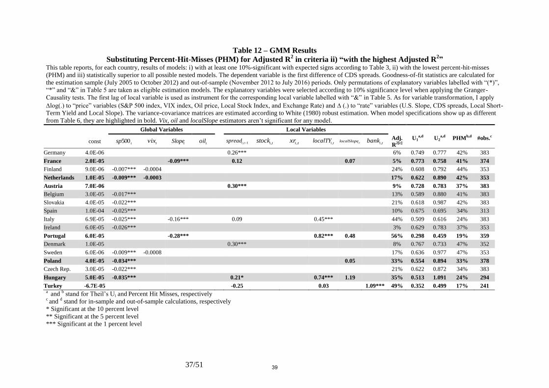
37/51
Table 12 – GMM Results
Substituting Percent-Hit-Misses (PHM) for Adjusted R2 in criteria ii) “with the highest Adjusted R
2”
This table reports, for each country, results of models: i) with at least one 10%-significant with expected signs according to Table 3, ii) with the lowest percent-hit-misses
(PHM) and iii) statistically superior to all possible nested models. The dependent variable is the first difference of CDS spreads. Goodness-of-fit statistics are calculated for
the estimation sample (July 2005 to October 2012) and out-of-sample (November 2012 to July 2016) periods. Only permutations of explanatory variables labelled with “(*)”,
“*” and “&” in Table 5 are taken as eligible estimation models. The explanatory variables were selected according to 10% significance level when applying the Granger-
Causality tests. The first lag of local variable is used as instrument for the corresponding local variable labelled with “&” in Table 5. As for variable transformation, I apply
log(.) to “price” variables (S&P 500 index, VIX index, Oil price, Local Stock Index, and Exchange Rate) and (.) to “rate” variables (U.S. Slope, CDS spreads, Local Short-
Term Yield and Local Slope). The variance-covariance matrices are estimated according to White (1980) robust estimation. When model specifications show up as different
from Table 6, they are highlighted in bold. Vix, oil and localSlope estimators aren’t significant for any model.
Global Variables Local Variables
const tsp500 tvix
tSlope toil 1, tispread
tistock ,
tixr ,
tilocalTY ,
tilocalSlope,
tibank , Adj.
R2[c] U1
a,d U2a,d PHMb,d #obs.c
Germany 4.0E-06 0.26*** 6% 0.749 0.777 42% 383
France 2.0E-05 -0.09*** 0.12 0.07 5% 0.773 0.758 41% 374
Finland 9.0E-06 -0.007*** -0.0004 24% 0.608 0.792 44% 353
Netherlands 1.0E-05 -0.009*** -0.0003 17% 0.622 0.890 42% 353
Austria 7.0E-06 0.30*** 9% 0.728 0.783 37% 383
Belgium 3.0E-05 -0.017*** 13% 0.589 0.880 41% 383
Slovakia 4.0E-05 -0.022*** 21% 0.618 0.987 42% 383
Spain 1.0E-04 -0.025*** 10% 0.675 0.695 34% 313
Italy 6.9E-05 -0.025*** -0.16*** 0.09 0.45*** 44% 0.509 0.616 24% 383
Ireland 6.0E-05 -0.026*** 3% 0.629 0.783 37% 353
Portugal 6.0E-05 -0.28*** 0.82*** 0.48 56% 0.298 0.459 19% 359
Denmark 1.0E-05 0.30*** 8% 0.767 0.733 47% 352
Sweden 6.0E-06 -0.009*** -0.0008 17% 0.636 0.977 47% 353
Poland 4.0E-05 -0.034*** 0.05 33% 0.554 0.894 33% 378
Czech Rep. 3.0E-05 -0.022*** 21% 0.622 0.872 34% 383
Hungary 5.0E-05 -0.035*** 0.21* 0.74*** 1.19 35% 0.513 1.091 24% 294
Turkey -6.7E-05 -0.25 0.03 1.09*** 49% 0.352 0.499 17% 241 a and
b stand for Theil’s Ui and
Percent Hit Misses, respectively
c and
d stand for in-sample and out-of-sample calculations, respectively
* Significant at the 10 percent level
** Significant at the 5 percent level
*** Significant at the 1 percent level
39
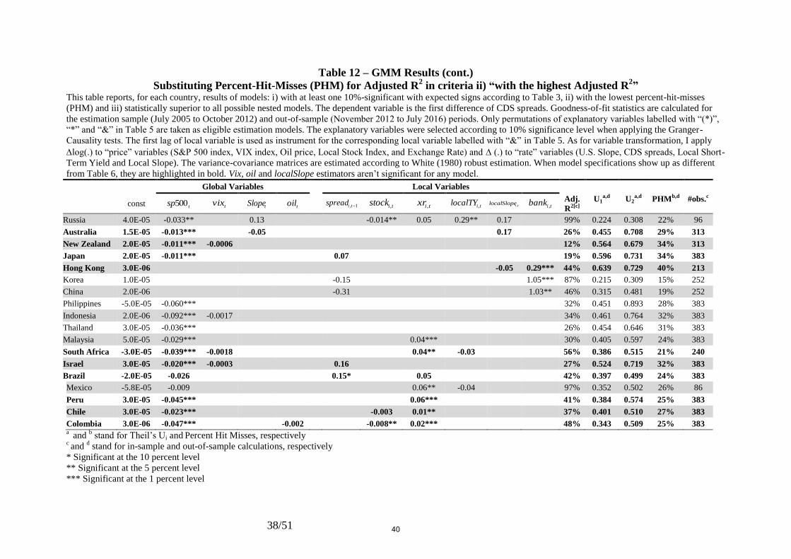
38/51
Table 12 – GMM Results (cont.)
Substituting Percent-Hit-Misses (PHM) for Adjusted R2 in criteria ii) “with the highest Adjusted R
2”
This table reports, for each country, results of models: i) with at least one 10%-significant with expected signs according to Table 3, ii) with the lowest percent-hit-misses
(PHM) and iii) statistically superior to all possible nested models. The dependent variable is the first difference of CDS spreads. Goodness-of-fit statistics are calculated for
the estimation sample (July 2005 to October 2012) and out-of-sample (November 2012 to July 2016) periods. Only permutations of explanatory variables labelled with “(*)”,
“*” and “&” in Table 5 are taken as eligible estimation models. The explanatory variables were selected according to 10% significance level when applying the Granger-
Causality tests. The first lag of local variable is used as instrument for the corresponding local variable labelled with “&” in Table 5. As for variable transformation, I apply
log(.) to “price” variables (S&P 500 index, VIX index, Oil price, Local Stock Index, and Exchange Rate) and (.) to “rate” variables (U.S. Slope, CDS spreads, Local Short-
Term Yield and Local Slope). The variance-covariance matrices are estimated according to White (1980) robust estimation. When model specifications show up as different
from Table 6, they are highlighted in bold. Vix, oil and localSlope estimators aren’t significant for any model.
Global Variables Local Variables
const tsp500 tvix
tSlope toil 1, tispread
tistock ,
tixr ,
tilocalTY ,
tilocalSlope,
tibank , Adj.
R2[c] U1
a,d U2a,d PHMb,d #obs.c
Russia 4.0E-05 -0.033** 0.13 -0.014** 0.05 0.29** 0.17 99% 0.224 0.308 22% 96
Australia 1.5E-05 -0.013*** -0.05 0.17 26% 0.455 0.708 29% 313
New Zealand 2.0E-05 -0.011*** -0.0006 12% 0.564 0.679 34% 313
Japan 2.0E-05 -0.011*** 0.07 19% 0.596 0.731 34% 383
Hong Kong 3.0E-06 -0.05 0.29*** 44% 0.639 0.729 40% 213
Korea 1.0E-05 -0.15 1.05*** 87% 0.215 0.309 15% 252
China 2.0E-06 -0.31 1.03** 46% 0.315 0.481 19% 252
Philippines -5.0E-05 -0.060*** 32% 0.451 0.893 28% 383
Indonesia 2.0E-06 -0.092*** -0.0017 34% 0.461 0.764 32% 383
Thailand 3.0E-05 -0.036*** 26% 0.454 0.646 31% 383
Malaysia 5.0E-05 -0.029*** 0.04*** 30% 0.405 0.597 24% 383
South Africa -3.0E-05 -0.039*** -0.0018 0.04** -0.03 56% 0.386 0.515 21% 240
Israel 3.0E-05 -0.020*** -0.0003 0.16 27% 0.524 0.719 32% 383
Brazil -2.0E-05 -0.026 0.15* 0.05 42% 0.397 0.499 24% 383
Mexico -5.8E-05 -0.009 0.06** -0.04 97% 0.352 0.502 26% 86
Peru 3.0E-05 -0.045*** 0.06*** 41% 0.384 0.574 25% 383
Chile 3.0E-05 -0.023*** -0.003 0.01** 37% 0.401 0.510 27% 383
Colombia 3.0E-06 -0.047*** -0.002 -0.008** 0.02*** 48% 0.343 0.509 25% 383 a and
b stand for Theil’s Ui and
Percent Hit Misses, respectively
c and
d stand for in-sample and out-of-sample calculations, respectively
* Significant at the 10 percent level
** Significant at the 5 percent level
*** Significant at the 1 percent level
40
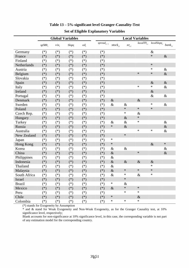
39/51
Table 13 – 5%-significant level Granger-Causality-Test
Set of Eligible Explanatory Variables
Global Variables Local Variables
tsp500 tvix
tSlope toil
1, tispread
tistock ,
tixr , tilocalTY ,
tilocalSlope,
tibank ,
Germany (*) (*) (*) (*) (*) &
France (*) (*) (*) (*) (*) * &
Finland (*) (*) (*) (*) (*)
Netherlands (*) (*) (*) (*) (*) *
Austria (*) (*) (*) (*) (*) * &
Belgium (*) (*) (*) (*) (*) * * &
Slovakia (*) (*) (*) (*) (*)
Spain (*) (*) (*) (*) (*) & &
Italy (*) (*) (*) (*) (*) * * &
Ireland (*) (*) (*) (*) (*) &
Portugal (*) (*) (*) (*) (*) & &
Denmark (*) (*) (*) (*) (*) & &
Sweden (*) (*) (*) (*) (*) & & * &
Poland (*) (*) (*) (*) (*) * * *
Czech Rep. (*) (*) (*) (*) (*) * &
Hungary (*) (*) (*) (*) (*) & *
Turkey (*) (*) (*) (*) (*) & & * &
Russia (*) (*) (*) (*) (*) * & &
Australia (*) (*) (*) (*) (*) * * &
New Zealand (*) (*) (*) (*) (*) *
Japan (*) (*) (*) (*) (*) *
Hong Kong (*) (*) (*) (*) (*) * & *
Korea (*) (*) (*) (*) (*) & & &
China (*) (*) (*) (*) (*) & * &
Philippines (*) (*) (*) (*) (*) &
Indonesia (*) (*) (*) (*) (*) & & & &
Thailand (*) (*) (*) (*) (*) & *
Malaysia (*) (*) (*) (*) (*) & * * *
South Africa (*) (*) (*) (*) (*) & * & *
Israel (*) (*) (*) (*) (*) *
Brazil (*) (*) (*) (*) (*) * &
Mexico (*) (*) (*) (*) (*) & * *
Peru (*) (*) (*) (*) (*) * *
Chile (*) (*) (*) (*) (*) * &
Colombia (*) (*) (*) (*) (*) * * * (*) stands for Exogeneity by Assumption
* and & stand for Weak Exogeneity and Non-Weak Exogeneity, as for the Granger Causality test, at 10%
significance level, respectively;
Blank accounts for non-significance at 10% significance level, in this case, the corresponding variable is not part
of any estimation model for the corresponding country.
41
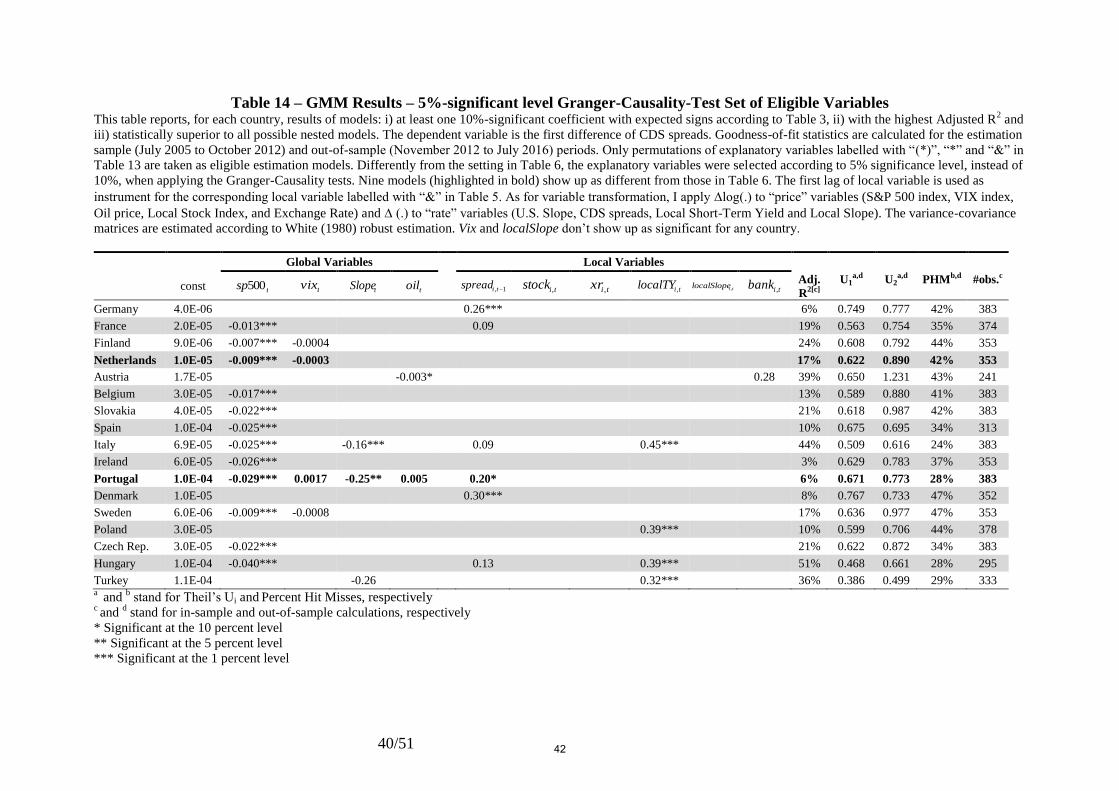
40/51
Table 14 – GMM Results – 5%-significant level Granger-Causality-Test Set of Eligible Variables This table reports, for each country, results of models: i) at least one 10%-significant coefficient with expected signs according to Table 3, ii) with the highest Adjusted R
2 and
iii) statistically superior to all possible nested models. The dependent variable is the first difference of CDS spreads. Goodness-of-fit statistics are calculated for the estimation
sample (July 2005 to October 2012) and out-of-sample (November 2012 to July 2016) periods. Only permutations of explanatory variables labelled with “(*)”, “*” and “&” in
Table 13 are taken as eligible estimation models. Differently from the setting in Table 6, the explanatory variables were selected according to 5% significance level, instead of
10%, when applying the Granger-Causality tests. Nine models (highlighted in bold) show up as different from those in Table 6. The first lag of local variable is used as
instrument for the corresponding local variable labelled with “&” in Table 5. As for variable transformation, I apply log(.) to “price” variables (S&P 500 index, VIX index,
Oil price, Local Stock Index, and Exchange Rate) and (.) to “rate” variables (U.S. Slope, CDS spreads, Local Short-Term Yield and Local Slope). The variance-covariance
matrices are estimated according to White (1980) robust estimation. Vix and localSlope don’t show up as significant for any country.
Global Variables Local Variables
const tsp500 tvix
tSlope toil 1, tispread
tistock ,
tixr ,
tilocalTY ,
tilocalSlope,
tibank , Adj.
R2[c] U1
a,d U2a,d PHMb,d #obs.c
Germany 4.0E-06 0.26*** 6% 0.749 0.777 42% 383
France 2.0E-05 -0.013*** 0.09 19% 0.563 0.754 35% 374
Finland 9.0E-06 -0.007*** -0.0004 24% 0.608 0.792 44% 353
Netherlands 1.0E-05 -0.009*** -0.0003 17% 0.622 0.890 42% 353
Austria 1.7E-05 -0.003* 0.28 39% 0.650 1.231 43% 241
Belgium 3.0E-05 -0.017*** 13% 0.589 0.880 41% 383
Slovakia 4.0E-05 -0.022*** 21% 0.618 0.987 42% 383
Spain 1.0E-04 -0.025*** 10% 0.675 0.695 34% 313
Italy 6.9E-05 -0.025*** -0.16*** 0.09 0.45*** 44% 0.509 0.616 24% 383
Ireland 6.0E-05 -0.026*** 3% 0.629 0.783 37% 353
Portugal 1.0E-04 -0.029*** 0.0017 -0.25** 0.005 0.20* 6% 0.671 0.773 28% 383
Denmark 1.0E-05 0.30*** 8% 0.767 0.733 47% 352
Sweden 6.0E-06 -0.009*** -0.0008 17% 0.636 0.977 47% 353
Poland 3.0E-05 0.39*** 10% 0.599 0.706 44% 378
Czech Rep. 3.0E-05 -0.022*** 21% 0.622 0.872 34% 383
Hungary 1.0E-04 -0.040*** 0.13 0.39*** 51% 0.468 0.661 28% 295
Turkey 1.1E-04 -0.26 0.32*** 36% 0.386 0.499 29% 333 a and
b stand for Theil’s Ui and
Percent Hit Misses, respectively
c and
d stand for in-sample and out-of-sample calculations, respectively
* Significant at the 10 percent level
** Significant at the 5 percent level
*** Significant at the 1 percent level
42
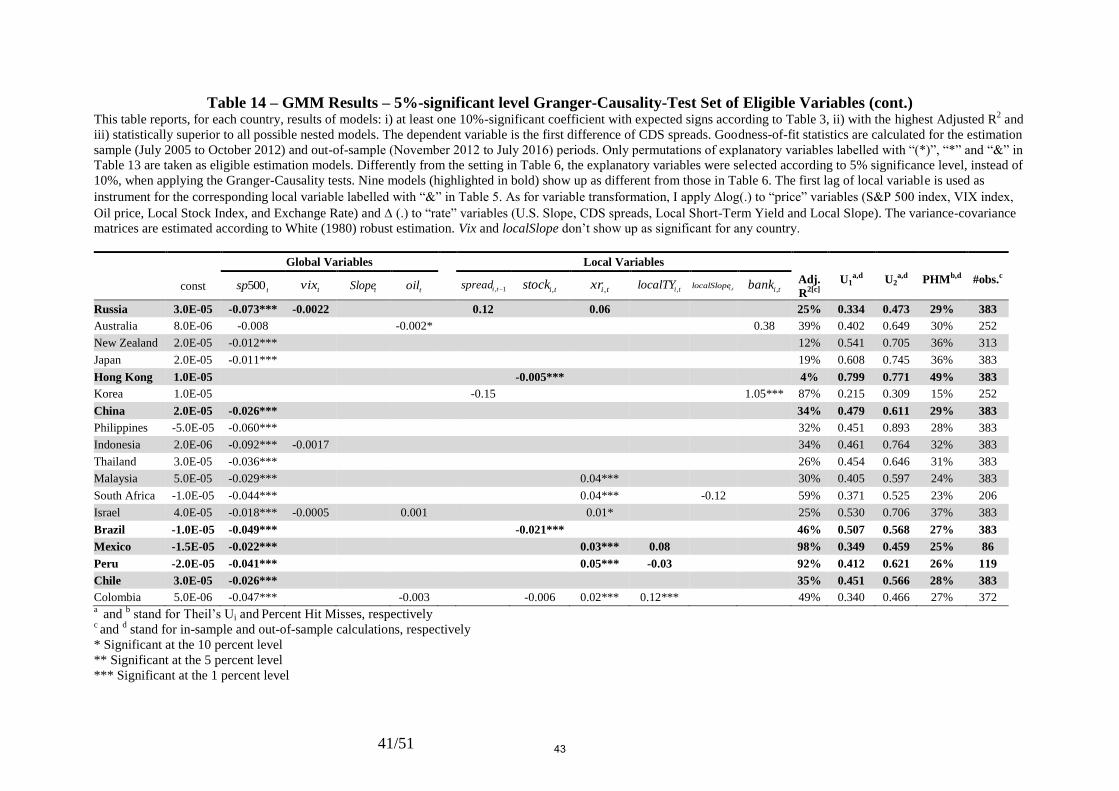
41/51
Table 14 – GMM Results – 5%-significant level Granger-Causality-Test Set of Eligible Variables (cont.) This table reports, for each country, results of models: i) at least one 10%-significant coefficient with expected signs according to Table 3, ii) with the highest Adjusted R
2 and
iii) statistically superior to all possible nested models. The dependent variable is the first difference of CDS spreads. Goodness-of-fit statistics are calculated for the estimation
sample (July 2005 to October 2012) and out-of-sample (November 2012 to July 2016) periods. Only permutations of explanatory variables labelled with “(*)”, “*” and “&” in
Table 13 are taken as eligible estimation models. Differently from the setting in Table 6, the explanatory variables were selected according to 5% significance level, instead of
10%, when applying the Granger-Causality tests. Nine models (highlighted in bold) show up as different from those in Table 6. The first lag of local variable is used as
instrument for the corresponding local variable labelled with “&” in Table 5. As for variable transformation, I apply log(.) to “price” variables (S&P 500 index, VIX index,
Oil price, Local Stock Index, and Exchange Rate) and (.) to “rate” variables (U.S. Slope, CDS spreads, Local Short-Term Yield and Local Slope). The variance-covariance
matrices are estimated according to White (1980) robust estimation. Vix and localSlope don’t show up as significant for any country.
Global Variables Local Variables
const tsp500 tvix
tSlope toil 1, tispread
tistock ,
tixr ,
tilocalTY ,
tilocalSlope,
tibank , Adj.
R2[c] U1
a,d U2a,d PHMb,d #obs.c
Russia 3.0E-05 -0.073*** -0.0022 0.12 0.06 25% 0.334 0.473 29% 383
Australia 8.0E-06 -0.008 -0.002* 0.38 39% 0.402 0.649 30% 252
New Zealand 2.0E-05 -0.012*** 12% 0.541 0.705 36% 313
Japan 2.0E-05 -0.011*** 19% 0.608 0.745 36% 383
Hong Kong 1.0E-05 -0.005*** 4% 0.799 0.771 49% 383
Korea 1.0E-05 -0.15 1.05*** 87% 0.215 0.309 15% 252
China 2.0E-05 -0.026*** 34% 0.479 0.611 29% 383
Philippines -5.0E-05 -0.060*** 32% 0.451 0.893 28% 383
Indonesia 2.0E-06 -0.092*** -0.0017 34% 0.461 0.764 32% 383
Thailand 3.0E-05 -0.036*** 26% 0.454 0.646 31% 383
Malaysia 5.0E-05 -0.029*** 0.04*** 30% 0.405 0.597 24% 383
South Africa -1.0E-05 -0.044*** 0.04*** -0.12 59% 0.371 0.525 23% 206
Israel 4.0E-05 -0.018*** -0.0005 0.001 0.01* 25% 0.530 0.706 37% 383
Brazil -1.0E-05 -0.049*** -0.021*** 46% 0.507 0.568 27% 383
Mexico -1.5E-05 -0.022*** 0.03*** 0.08 98% 0.349 0.459 25% 86
Peru -2.0E-05 -0.041*** 0.05*** -0.03 92% 0.412 0.621 26% 119
Chile 3.0E-05 -0.026*** 35% 0.451 0.566 28% 383
Colombia 5.0E-06 -0.047*** -0.003 -0.006 0.02*** 0.12*** 49% 0.340 0.466 27% 372 a and
b stand for Theil’s Ui and
Percent Hit Misses, respectively
c and
d stand for in-sample and out-of-sample calculations, respectively
* Significant at the 10 percent level
** Significant at the 5 percent level
*** Significant at the 1 percent level
43
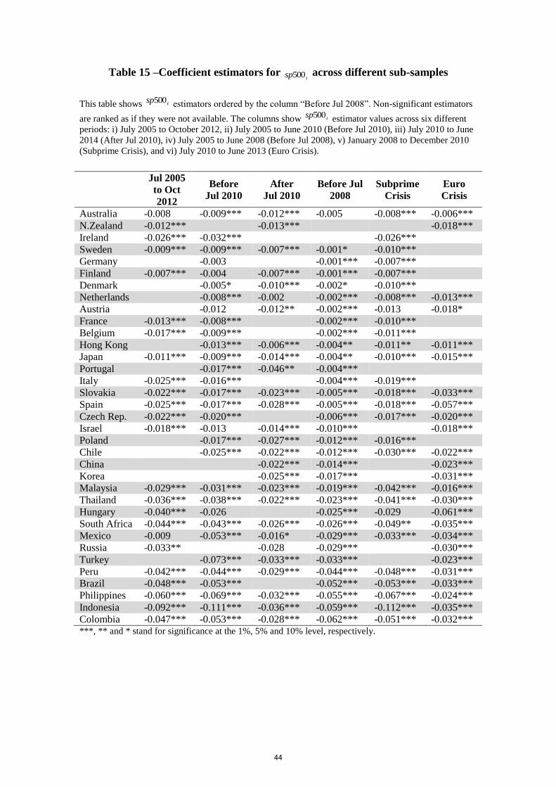
Table 15 –Coefficient estimators for tsp500 across different sub-samples
This table shows tsp500 estimators ordered by the column “Before Jul 2008”. Non-significant estimators
are ranked as if they were not available. The columns show tsp500 estimator values across six different
periods: i) July 2005 to October 2012, ii) July 2005 to June 2010 (Before Jul 2010), iii) July 2010 to June
2014 (After Jul 2010), iv) July 2005 to June 2008 (Before Jul 2008), v) January 2008 to December 2010
(Subprime Crisis), and vi) July 2010 to June 2013 (Euro Crisis).
Jul 2005
to Oct
2012
Before
Jul 2010
After
Jul 2010
Before Jul
2008
Subprime
Crisis
Euro
Crisis
Australia -0.008 -0.009*** -0.012*** -0.005 -0.008*** -0.006***
N.Zealand -0.012*** -0.013*** -0.018***
Ireland -0.026*** -0.032*** -0.026***
Sweden -0.009*** -0.009*** -0.007*** -0.001* -0.010***
Germany -0.003 -0.001*** -0.007***
Finland -0.007*** -0.004 -0.007*** -0.001*** -0.007***
Denmark -0.005* -0.010*** -0.002* -0.010***
Netherlands -0.008*** -0.002 -0.002*** -0.008*** -0.013***
Austria -0.012 -0.012** -0.002*** -0.013 -0.018*
France -0.013*** -0.008*** -0.002*** -0.010***
Belgium -0.017*** -0.009*** -0.002*** -0.011***
Hong Kong -0.013*** -0.006*** -0.004** -0.011** -0.011***
Japan -0.011*** -0.009*** -0.014*** -0.004** -0.010*** -0.015***
Portugal -0.017*** -0.046** -0.004***
Italy -0.025*** -0.016*** -0.004*** -0.019***
Slovakia -0.022*** -0.017*** -0.023*** -0.005*** -0.018*** -0.033***
Spain -0.025*** -0.017*** -0.028*** -0.005*** -0.018*** -0.057***
Czech Rep. -0.022*** -0.020*** -0.006*** -0.017*** -0.020***
Israel -0.018*** -0.013 -0.014*** -0.010*** -0.018***
Poland -0.017*** -0.027*** -0.012*** -0.016***
Chile -0.025*** -0.022*** -0.012*** -0.030*** -0.022***
China -0.022*** -0.014*** -0.023***
Korea -0.025*** -0.017*** -0.031***
Malaysia -0.029*** -0.031*** -0.023*** -0.019*** -0.042*** -0.016***
Thailand -0.036*** -0.038*** -0.022*** -0.023*** -0.041*** -0.030***
Hungary -0.040*** -0.026 -0.025*** -0.029 -0.061***
South Africa -0.044*** -0.043*** -0.026*** -0.026*** -0.049** -0.035***
Mexico -0.009 -0.053*** -0.016* -0.029*** -0.033*** -0.034***
Russia -0.033** -0.028 -0.029*** -0.030***
Turkey -0.073*** -0.033*** -0.033*** -0.023***
Peru -0.042*** -0.044*** -0.029*** -0.044*** -0.048*** -0.031***
Brazil -0.048*** -0.053*** -0.052*** -0.053*** -0.033***
Philippines -0.060*** -0.069*** -0.032*** -0.055*** -0.067*** -0.024***
Indonesia -0.092*** -0.111*** -0.036*** -0.059*** -0.112*** -0.035***
Colombia -0.047*** -0.053*** -0.028*** -0.062*** -0.051*** -0.032*** ***, ** and * stand for significance at the 1%, 5% and 10% level, respectively.
44
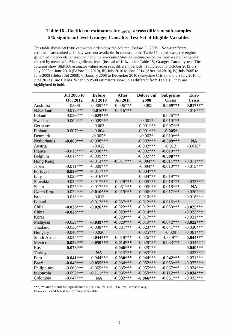
Table 16 –Coefficient estimators for tsp500 across different sub-samples
5%-significant level Granger-Causality-Test Set of Eligible Variables
This table shows S&P500 estimators ordered by the column “Before Jul 2008”. Non-significant
estimators are ranked as if they were not available. In contrast to the Table 15, in this case, the engine
generated the models corresponding to the associated S&P500 estimators below from a set of variables
elected by means of a 5%-significant level (instead of 10%, as for Table 15) Granger-Causality-test. The
columns show S&P500 estimator values across six different periods: i) July 2005 to October 2012, ii)
July 2005 to June 2010 (Before Jul 2010), iii) July 2010 to June 2014 (After Jul 2010), iv) July 2005 to
June 2008 (Before Jul 2008), v) January 2008 to December 2010 (Subprime Crisis), and vi) July 2010 to
June 2013 (Euro Crisis). When S&P500 estimators show up as different from Table 15, they are
highlighted in bold.
Jul 2005 to
Oct 2012
Before
Jul 2010
After
Jul 2010
Before Jul
2008
Subprime
Crisis
Euro
Crisis
Australia -0.008 -0.009*** -0.006*** -0.005 -0.009*** -0.017***
N.Zealand -0.012*** -0.010** -0.016*** -0.018***
Ireland -0.026*** -0.025*** -0.026***
Sweden -0.009*** -0.009*** -0.001* -0.010***
Germany -0.003 -0.001*** -0.007***
Finland -0.007*** -0.004 -0.001*** -0.005*
Denmark -0.005* -0.002* -0.010***
Netherlands -0.009*** -0.008*** -0.002*** -0.009*** NA
Austria -0.012 -0.002*** -0.013 -0.018*
France -0.013*** -0.008*** -0.002*** -0.010***
Belgium -0.017*** -0.009*** -0.002*** -0.008***
Hong Kong -0.013*** -0.011*** -0.004** -0.011*** -0.011***
Japan -0.011*** -0.009*** -0.004** -0.010*** -0.015***
Portugal -0.029*** -0.017*** -0.004***
Italy -0.025*** -0.016*** -0.004*** -0.019***
Slovakia -0.022*** -0.017*** -0.029*** -0.005*** -0.018*** -0.033***
Spain -0.025*** -0.017*** -0.051*** -0.005*** -0.018*** NA
Czech Rep. -0.022*** -0.016*** -0.019*** -0.006*** -0.017*** -0.020***
Israel -0.018*** -0.013 -0.010*** -0.018***
Poland -0.017*** -0.037*** -0.012*** -0.016***
Chile -0.026*** -0.026*** -0.022*** -0.012*** -0.030*** -0.025***
China -0.026*** -0.023*** -0.014*** -0.023***
Korea -0.029*** -0.017*** -0.031***
Malaysia -0.029*** -0.039*** -0.029*** -0.019*** -0.042*** -0.022***
Thailand -0.036*** -0.038*** -0.031*** -0.023*** -0.041*** -0.030***
Hungary -0.040*** -0.026 -0.025*** -0.029 -0.061***
South Africa -0.044*** -0.044*** -0.018*** -0.026*** -0.049** -0.044***
Mexico -0.022*** -0.050*** -0.014*** -0.029*** -0.033*** -0.034***
Russia -0.073*** -0.046*** -0.029*** -0.049***
Turkey NA -0.013*** -0.033*** -0.023***
Peru -0.041*** -0.044*** -0.030*** -0.044*** -0.042*** -0.031***
Brazil -0.049*** -0.055*** -0.034*** -0.052*** -0.053*** -0.033***
Philippines -0.060*** -0.069*** -0.035*** -0.055*** -0.067*** -0.024***
Indonesia -0.092*** -0.111*** -0.036*** -0.059*** -0.112*** -0.034***
Colombia -0.047*** NA -0.032*** -0.066*** -0.051*** -0.032***
***, ** and * stand for significance at the 1%, 5% and 10% level, respectively;
Blank cells and NA stand for “non-available”.
45
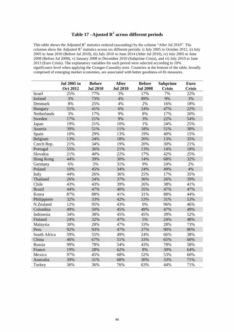
Table 17 –Ajusted R2 across different periods
This table shows the Adjusted R2 statistics ordered (ascending) by the column “After Jul 2010”. The
columns show the Adjusted R2 statistics across six different periods: i) July 2005 to October 2012, ii) July
2005 to June 2010 (Before Jul 2010), iii) July 2010 to June 2014 (After Jul 2010), iv) July 2005 to June
2008 (Before Jul 2008), v) January 2008 to December 2010 (Subprime Crisis), and vi) July 2010 to June
2013 (Euro Crisis). The explanatory variables for each period were selected according to 10%
significance level when applying the Granger-Causality tests. Countries at the bottom of the table, broadly
comprised of emerging market economies, are associated with better goodness-of-fit measures.
Jul 2005 to
Oct 2012
Before
Jul 2010
After
Jul 2010
Before
Jul 2008
Subprime
Crisis
Euro
Crisis
Israel 25% 77% 3% 17% 7% 22%
Ireland 3% 73% 4% 89% 9% 3%
Denmark 8% 25% 4% 2% 16% 18%
Hungary 51% 41% 6% 24% 47% 22%
Netherlands 3% 17% 9% 8% 17% 20%
Sweden 17% 21% 9% 3% 22% 54%
Japan 19% 21% 10% 1% 24% 25%
Austria 39% 51% 11% 18% 51% 38%
Spain 10% 29% 13% 19% 40% 15%
Belgium 13% 24% 18% 20% 13% 35%
Czech Rep. 21% 34% 19% 20% 30% 21%
Portugal 55% 36% 21% 13% 14% 18%
Slovakia 21% 40% 22% 17% 42% 25%
Hong Kong 44% 39% 30% 14% 68% 32%
Germany 6% 5% 31% 9% 24% 2%
Poland 10% 45% 34% 24% 49% 4%
Italy 44% 26% 36% 25% 17% 35%
Thailand 26% 24% 37% 36% 26% 39%
Chile 43% 43% 39% 26% 38% 41%
Brazil 44% 47% 40% 35% 47% 47%
Korea 87% 88% 41% 31% 88% 44%
Philippines 32% 33% 42% 53% 31% 53%
N.Zealand 12% 95% 43% 0% 96% 46%
Colombia 49% 50% 45% 49% 47% 49%
Indonesia 34% 38% 45% 45% 39% 52%
Finland 24% 32% 47% 5% 24% 48%
Malaysia 30% 28% 47% 33% 28% 73%
Peru 92% 93% 47% 27% 90% 80%
South Africa 59% 55% 49% 24% 66% 38%
China 46% 67% 51% 33% 65% 60%
Russia 99% 78% 54% 43% 78% 58%
France 19% 28% 62% 8% 30% 64%
Mexico 97% 45% 68% 52% 53% 60%
Australia 39% 31% 68% 30% 33% 71%
Turkey 36% 36% 76% 63% 44% 71%
46
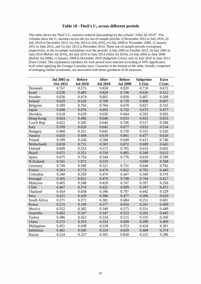
Table 18 –Theil’s U1 across different periods
This table shows the Theil’s U1 statistics ordered (descending) by the column “After Jul 2010”. The
columns show the U1 statistics across the six out-of-sample periods: i) November 2012 to July 2016, ii)
July 2010 to December 2012, iii) July 2014 to July 2016, iv) July 2008 to November 2009, v) January
2011 to June 2012, and vi) July 2013 to December 2014. These out-of-sample periods correspond,
respectively, to the in-sample estimations over the periods: i) July 2005 to October 2012, ii) July 2005 to
June 2010 (Before Jul 2010), iii) July 2010 to June 2014 (After Jul 2010), iv) July 2005 to June 2008
(Before Jul 2008), v) January 2008 to December 2010 (Subprime Crisis), and vi) July 2010 to June 2013
(Euro Crisis). The explanatory variables for each period were selected according to 10% significance
level when applying the Granger-Causality tests. Countries at the bottom of the table, broadly comprised
of emerging market economies, are associated with better goodness-of-fit measures.
Jul 2005 to
Oct 2012
Before
Jul 2010
After
Jul 2010
Before
Jul 2008
Subprime
Crisis
Euro
Crisis
Denmark 0.767 0.575 0.858 0.920 0.710 0.672
Israel 0.530 0.483 0.829 0.746 0.630 0.512
Sweden 0.636 0.474 0.805 0.838 0.467 0.568
Ireland 0.629 0.520 0.790 0.739 0.898 0.667
Belgium 0.589 0.765 0.784 0.678 0.827 0.535
Japan 0.608 0.676 0.692 0.732 0.673 0.477
Slovakia 0.618 0.629 0.650 0.664 0.593 0.650
Hong Kong 0.643 0.486 0.646 0.633 0.425 0.653
Czech Rep. 0.622 0.585 0.646 0.706 0.517 0.598
Italy 0.509 0.820 0.642 0.677 0.832 0.534
Hungary 0.468 0.351 0.641 0.739 0.331 0.520
Austria 0.650 0.498 0.619 0.841 0.477 0.620
Poland 0.599 0.436 0.584 0.649 0.413 0.746
Netherlands 0.818 0.721 0.583 0.872 0.689 0.645
Finland 0.608 0.553 0.571 0.705 0.633 0.602
Brazil 0.471 0.351 0.550 0.485 0.340 0.612
Spain 0.675 0.754 0.544 0.776 0.619 0.599
N.Zealand 0.541 1.072 0.533 - 0.690 0.568
Germany 0.749 0.580 0.521 0.731 0.648 0.782
France 0.563 0.773 0.479 0.822 0.705 0.443
Colombia 0.340 0.359 0.470 0.447 0.340 0.576
Portugal 0.305 0.651 0.470 0.798 0.794 0.417
Malaysia 0.405 0.348 0.428 0.747 0.397 0.256
Chile 0.467 0.374 0.425 0.699 0.397 0.471
Thailand 0.454 0.438 0.396 0.707 0.442 0.529
Peru 0.415 0.439 0.386 0.477 0.396 0.620
South Africa 0.371 0.371 0.381 0.684 0.251 0.601
Korea 0.215 0.199 0.377 0.816 0.201 0.499
Mexico 0.352 0.382 0.348 0.575 0.331 0.449
Australia 0.402 0.347 0.347 0.553 0.265 0.445
Turkey 0.386 0.422 0.334 0.515 0.335 0.300
China 0.315 0.353 0.333 0.688 0.290 0.499
Philippines 0.451 0.438 0.318 0.553 0.424 0.361
Indonesia 0.461 0.500 0.310 0.629 0.488 0.374
Russia 0.224 0.237 0.305 0.838 0.225 0.286
47
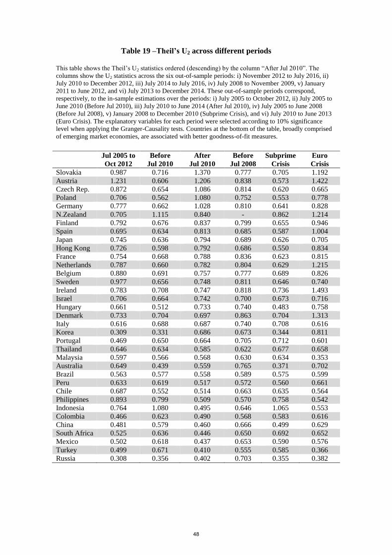
Table 19 –Theil’s U2 across different periods
This table shows the Theil’s U2 statistics ordered (descending) by the column “After Jul 2010”. The
columns show the U2 statistics across the six out-of-sample periods: i) November 2012 to July 2016, ii)
July 2010 to December 2012, iii) July 2014 to July 2016, iv) July 2008 to November 2009, v) January
2011 to June 2012, and vi) July 2013 to December 2014. These out-of-sample periods correspond,
respectively, to the in-sample estimations over the periods: i) July 2005 to October 2012, ii) July 2005 to
June 2010 (Before Jul 2010), iii) July 2010 to June 2014 (After Jul 2010), iv) July 2005 to June 2008
(Before Jul 2008), v) January 2008 to December 2010 (Subprime Crisis), and vi) July 2010 to June 2013
(Euro Crisis). The explanatory variables for each period were selected according to 10% significance
level when applying the Granger-Causality tests. Countries at the bottom of the table, broadly comprised
of emerging market economies, are associated with better goodness-of-fit measures.
Jul 2005 to
Oct 2012
Before
Jul 2010
After
Jul 2010
Before
Jul 2008
Subprime
Crisis
Euro
Crisis
Slovakia 0.987 0.716 1.370 0.777 0.705 1.192
Austria 1.231 0.606 1.206 0.838 0.573 1.422
Czech Rep. 0.872 0.654 1.086 0.814 0.620 0.665
Poland 0.706 0.562 1.080 0.752 0.553 0.778
Germany 0.777 0.662 1.028 0.810 0.641 0.828
N.Zealand 0.705 1.115 0.840 - 0.862 1.214
Finland 0.792 0.676 0.837 0.799 0.655 0.946
Spain 0.695 0.634 0.813 0.685 0.587 1.004
Japan 0.745 0.636 0.794 0.689 0.626 0.705
Hong Kong 0.726 0.598 0.792 0.686 0.550 0.834
France 0.754 0.668 0.788 0.836 0.623 0.815
Netherlands 0.787 0.660 0.782 0.804 0.629 1.215
Belgium 0.880 0.691 0.757 0.777 0.689 0.826
Sweden 0.977 0.656 0.748 0.811 0.646 0.740
Ireland 0.783 0.708 0.747 0.818 0.736 1.493
Israel 0.706 0.664 0.742 0.700 0.673 0.716
Hungary 0.661 0.512 0.733 0.740 0.483 0.758
Denmark 0.733 0.704 0.697 0.863 0.704 1.313
Italy 0.616 0.688 0.687 0.740 0.708 0.616
Korea 0.309 0.331 0.686 0.673 0.344 0.811
Portugal 0.469 0.650 0.664 0.705 0.712 0.601
Thailand 0.646 0.634 0.585 0.622 0.677 0.658
Malaysia 0.597 0.566 0.568 0.630 0.634 0.353
Australia 0.649 0.439 0.559 0.765 0.371 0.702
Brazil 0.563 0.577 0.558 0.589 0.575 0.599
Peru 0.633 0.619 0.517 0.572 0.560 0.661
Chile 0.687 0.552 0.514 0.663 0.635 0.564
Philippines 0.893 0.799 0.509 0.570 0.758 0.542
Indonesia 0.764 1.080 0.495 0.646 1.065 0.553
Colombia 0.466 0.623 0.490 0.568 0.583 0.616
China 0.481 0.579 0.460 0.666 0.499 0.629
South Africa 0.525 0.636 0.446 0.650 0.692 0.652
Mexico 0.502 0.618 0.437 0.653 0.590 0.576
Turkey 0.499 0.671 0.410 0.555 0.585 0.366
Russia 0.308 0.356 0.402 0.703 0.355 0.382
48
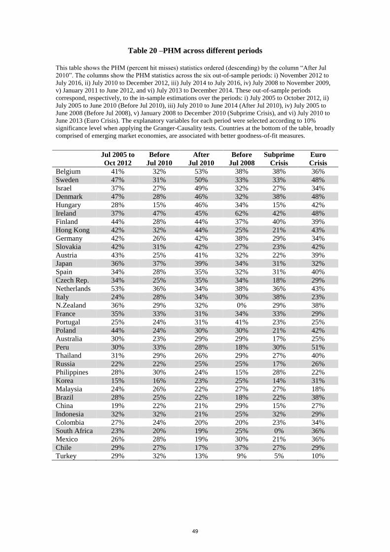
Table 20 –PHM across different periods
This table shows the PHM (percent hit misses) statistics ordered (descending) by the column “After Jul
2010”. The columns show the PHM statistics across the six out-of-sample periods: i) November 2012 to
July 2016, ii) July 2010 to December 2012, iii) July 2014 to July 2016, iv) July 2008 to November 2009,
v) January 2011 to June 2012, and vi) July 2013 to December 2014. These out-of-sample periods
correspond, respectively, to the in-sample estimations over the periods: i) July 2005 to October 2012, ii)
July 2005 to June 2010 (Before Jul 2010), iii) July 2010 to June 2014 (After Jul 2010), iv) July 2005 to
June 2008 (Before Jul 2008), v) January 2008 to December 2010 (Subprime Crisis), and vi) July 2010 to
June 2013 (Euro Crisis). The explanatory variables for each period were selected according to 10%
significance level when applying the Granger-Causality tests. Countries at the bottom of the table, broadly
comprised of emerging market economies, are associated with better goodness-of-fit measures.
Jul 2005 to
Oct 2012
Before
Jul 2010
After
Jul 2010
Before
Jul 2008
Subprime
Crisis
Euro
Crisis
Belgium 41% 32% 53% 38% 38% 36%
Sweden 47% 31% 50% 33% 33% 48%
Israel 37% 27% 49% 32% 27% 34%
Denmark 47% 28% 46% 32% 38% 48%
Hungary 28% 15% 46% 34% 15% 42%
Ireland 37% 47% 45% 62% 42% 48%
Finland 44% 28% 44% 37% 40% 39%
Hong Kong 42% 32% 44% 25% 21% 43%
Germany 42% 26% 42% 38% 29% 34%
Slovakia 42% 31% 42% 27% 23% 42%
Austria 43% 25% 41% 32% 22% 39%
Japan 36% 37% 39% 34% 31% 32%
Spain 34% 28% 35% 32% 31% 40%
Czech Rep. 34% 25% 35% 34% 18% 29%
Netherlands 53% 36% 34% 38% 36% 43%
Italy 24% 28% 34% 30% 38% 23%
N.Zealand 36% 29% 32% 0% 29% 38%
France 35% 33% 31% 34% 33% 29%
Portugal 25% 24% 31% 41% 23% 25%
Poland 44% 24% 30% 30% 21% 42%
Australia 30% 23% 29% 29% 17% 25%
Peru 30% 33% 28% 18% 30% 51%
Thailand 31% 29% 26% 29% 27% 40%
Russia 22% 22% 25% 25% 17% 26%
Philippines 28% 30% 24% 15% 28% 22%
Korea 15% 16% 23% 25% 14% 31%
Malaysia 24% 26% 22% 27% 27% 18%
Brazil 28% 25% 22% 18% 22% 38%
China 19% 22% 21% 29% 15% 27%
Indonesia 32% 32% 21% 25% 32% 29%
Colombia 27% 24% 20% 20% 23% 34%
South Africa 23% 20% 19% 25% 0% 36%
Mexico 26% 28% 19% 30% 21% 36%
Chile 29% 27% 17% 37% 27% 29%
Turkey 29% 32% 13% 9% 5% 10%
49
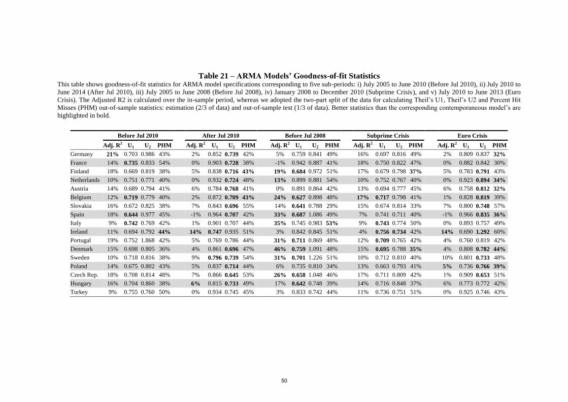
Table 21 – ARMA Models’ Goodness-of-fit Statistics This table shows goodness-of-fit statistics for ARMA model specifications corresponding to five sub-periods: i) July 2005 to June 2010 (Before Jul 2010), ii) July 2010 to
June 2014 (After Jul 2010), iii) July 2005 to June 2008 (Before Jul 2008), iv) January 2008 to December 2010 (Subprime Crisis), and v) July 2010 to June 2013 (Euro
Crisis). The Adjusted R2 is calculated over the in-sample period, whereas we adopted the two-part split of the data for calculating Theil’s U1, Theil’s U2 and Percent Hit
Misses (PHM) out-of-sample statistics: estimation (2/3 of data) and out-of-sample test (1/3 of data). Better statistics than the corresponding contemporaneous model’s are
highlighted in bold.
Before Jul 2010 After Jul 2010 Before Jul 2008 Subprime Crisis Euro Crisis
Adj. R2 U1 U2 PHM Adj. R2 U1
U2 PHM Adj. R2 U1 U2 PHM
Adj. R2 U1 U2 PHM
Adj. R2 U1 U2 PHM
Germany 21% 0.703 0.986 43% 2% 0.852 0.739 42% 5% 0.759 0.841 49% 16% 0.697 0.816 49% 2% 0.809 0.837 32%
France 14% 0.735 0.833 54% 0% 0.903 0.728 38% -1% 0.942 0.887 41% 18% 0.750 0.822 47% 0% 0.882 0.842 30%
Finland 18% 0.669 0.819 38% 5% 0.838 0.716 43% 19% 0.684 0.972 51% 17% 0.679 0.798 37% 5% 0.783 0.791 43%
Netherlands 10% 0.751 0.771 40% 0% 0.932 0.724 48% 13% 0.899 0.881 54% 10% 0.752 0.767 40% 0% 0.923 0.894 34%
Austria 14% 0.689 0.794 41% 6% 0.784 0.768 41% 0% 0.891 0.864 42% 13% 0.694 0.777 45% 6% 0.758 0.812 32%
Belgium 12% 0.719 0.779 40% 2% 0.872 0.709 43% 24% 0.627 0.898 48% 17% 0.717 0.798 41% 1% 0.828 0.819 39%
Slovakia 16% 0.672 0.825 38% 7% 0.843 0.696 55% 14% 0.641 0.788 29% 15% 0.674 0.814 33% 7% 0.800 0.748 57%
Spain 18% 0.644 0.977 45% -1% 0.964 0.707 42% 33% 0.687 1.086 49% 7% 0.741 0.711 40% -1% 0.966 0.835 36%
Italy 9% 0.742 0.769 42% 1% 0.901 0.707 44% 35% 0.745 0.983 53% 9% 0.743 0.774 50% 0% 0.893 0.757 49%
Ireland 11% 0.694 0.792 44% 14% 0.747 0.935 51% 3% 0.842 0.845 51% 4% 0.756 0.734 42% 14% 0.690 1.292 60%
Portugal 19% 0.752 1.868 42% 5% 0.769 0.786 44% 31% 0.711 0.869 48% 12% 0.709 0.765 42% 4% 0.760 0.819 42%
Denmark 15% 0.698 0.805 36% 4% 0.861 0.696 47% 46% 0.759 1.091 48% 15% 0.695 0.788 35% 4% 0.808 0.782 44%
Sweden 10% 0.718 0.816 38% 9% 0.796 0.739 54% 31% 0.701 1.226 51% 10% 0.712 0.810 40% 10% 0.801 0.733 48%
Poland 14% 0.675 0.802 43% 5% 0.837 0.714 44% 6% 0.735 0.810 34% 13% 0.663 0.793 41% 5% 0.736 0.766 39%
Czech Rep. 18% 0.708 0.814 48% 7% 0.866 0.645 53% 26% 0.658 1.048 46% 17% 0.711 0.809 42% 1% 0.909 0.653 51%
Hungary 16% 0.704 0.860 38% 6% 0.815 0.733 49% 17% 0.642 0.748 39% 14% 0.716 0.848 37% 6% 0.773 0.772 42%
Turkey 9% 0.755 0.760 50% 0% 0.934 0.745 45% 3% 0.833 0.742 44% 11% 0.736 0.751 51% 0% 0.925 0.746 43%
50
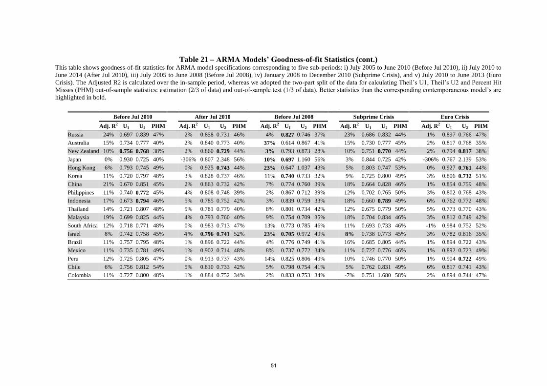
Table 21 – ARMA Models’ Goodness-of-fit Statistics (cont.) This table shows goodness-of-fit statistics for ARMA model specifications corresponding to five sub-periods: i) July 2005 to June 2010 (Before Jul 2010), ii) July 2010 to
June 2014 (After Jul 2010), iii) July 2005 to June 2008 (Before Jul 2008), iv) January 2008 to December 2010 (Subprime Crisis), and v) July 2010 to June 2013 (Euro
Crisis). The Adjusted R2 is calculated over the in-sample period, whereas we adopted the two-part split of the data for calculating Theil’s U1, Theil’s U2 and Percent Hit
Misses (PHM) out-of-sample statistics: estimation (2/3 of data) and out-of-sample test (1/3 of data). Better statistics than the corresponding contemporaneous model’s are
highlighted in bold.
Before Jul 2010 After Jul 2010 Before Jul 2008 Subprime Crisis Euro Crisis
Adj. R2 U1 U2 PHM Adj. R2 U1 U2 PHM Adj. R2 U1 U2 PHM Adj. R2 U1 U2 PHM Adj. R2 U1
U2 PHM
Russia 24% 0.697 0.839 47% 2% 0.858 0.731 46% 4% 0.827 0.746 37% 23% 0.686 0.832 44% 1% 0.897 0.766 47%
Australia 15% 0.734 0.777 40% 2% 0.840 0.773 40% 37% 0.614 0.867 41% 15% 0.730 0.777 45% 2% 0.817 0.768 35%
New Zealand 10% 0.756 0.768 38% 2% 0.860 0.729 44% 3% 0.793 0.873 28% 10% 0.751 0.770 44% 2% 0.794 0.817 38%
Japan 0% 0.930 0.725 40% -306% 0.807 2.348 56% 10% 0.697 1.160 56% 3% 0.844 0.725 42% -306% 0.767 2.139 53%
Hong Kong 6% 0.793 0.745 49% 0% 0.925 0.743 44% 23% 0.647 1.037 43% 5% 0.803 0.747 53% 0% 0.927 0.761 44%
Korea 11% 0.720 0.797 48% 3% 0.828 0.737 46% 11% 0.740 0.733 32% 9% 0.725 0.800 49% 3% 0.806 0.732 51%
China 21% 0.670 0.851 45% 2% 0.863 0.732 42% 7% 0.774 0.760 39% 18% 0.664 0.828 46% 1% 0.854 0.759 48%
Philippines 11% 0.740 0.772 45% 4% 0.808 0.748 39% 2% 0.867 0.712 39% 12% 0.702 0.765 50% 3% 0.802 0.768 43%
Indonesia 17% 0.673 0.794 46% 5% 0.785 0.752 42% 3% 0.839 0.759 33% 18% 0.660 0.789 49% 6% 0.762 0.772 48%
Thailand 14% 0.721 0.807 48% 5% 0.781 0.779 40% 8% 0.801 0.734 42% 12% 0.675 0.779 50% 5% 0.773 0.770 43%
Malaysia 19% 0.699 0.825 44% 4% 0.793 0.760 40% 9% 0.754 0.709 35% 18% 0.704 0.834 46% 3% 0.812 0.749 42%
South Africa 12% 0.718 0.771 48% 0% 0.983 0.713 47% 13% 0.773 0.785 46% 11% 0.693 0.733 46% -1% 0.984 0.752 52%
Israel 8% 0.742 0.758 45% 4% 0.796 0.741 52% 23% 0.705 0.972 49% 8% 0.738 0.773 45% 3% 0.782 0.816 35%
Brazil 11% 0.757 0.795 48% 1% 0.896 0.722 44% 4% 0.776 0.749 41% 16% 0.685 0.805 44% 1% 0.894 0.722 43%
Mexico 11% 0.735 0.781 49% 1% 0.902 0.714 48% 8% 0.737 0.772 34% 11% 0.727 0.776 46% 1% 0.892 0.723 49%
Peru 12% 0.725 0.805 47% 0% 0.913 0.737 43% 14% 0.825 0.806 49% 10% 0.746 0.770 50% 1% 0.904 0.722 49%
Chile 6% 0.756 0.812 54% 5% 0.810 0.733 42% 5% 0.798 0.754 41% 5% 0.762 0.831 49% 6% 0.817 0.741 43%
Colombia 11% 0.727 0.800 48% 1% 0.884 0.752 34% 2% 0.833 0.753 34% -7% 0.751 1.680 58% 2% 0.894 0.744 47%
51
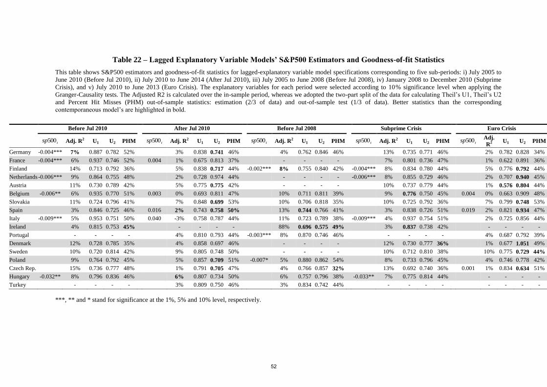
Table 22 – Lagged Explanatory Variable Models’ S&P500 Estimators and Goodness-of-fit Statistics
This table shows S&P500 estimators and goodness-of-fit statistics for lagged-explanatory variable model specifications corresponding to five sub-periods: i) July 2005 to
June 2010 (Before Jul 2010), ii) July 2010 to June 2014 (After Jul 2010), iii) July 2005 to June 2008 (Before Jul 2008), iv) January 2008 to December 2010 (Subprime
Crisis), and v) July 2010 to June 2013 (Euro Crisis). The explanatory variables for each period were selected according to 10% significance level when applying the
Granger-Causality tests. The Adjusted R2 is calculated over the in-sample period, whereas we adopted the two-part split of the data for calculating Theil’s U1, Theil’s U2
and Percent Hit Misses (PHM) out-of-sample statistics: estimation (2/3 of data) and out-of-sample test (1/3 of data). Better statistics than the corresponding
contemporaneous model’s are highlighted in bold.
Before Jul 2010 After Jul 2010 Before Jul 2008 Subprime Crisis Euro Crisis
tsp500 Adj. R2 U1 U2 PHM tsp500 Adj. R2 U1 U2 PHM tsp500 Adj. R2 U1 U2 PHM tsp500 Adj. R2 U1 U2 PHM tsp500Adj.
R2 U1 U2 PHM
Germany -0.004*** 7% 0.887 0.782 52% 3% 0.838 0.741 46% 4% 0.762 0.846 46% 13% 0.735 0.771 46% 2% 0.782 0.828 34%
France -0.004*** 6% 0.937 0.746 52% 0.004 1% 0.675 0.813 37% - - - - 7% 0.801 0.736 47% 1% 0.622 0.891 36%
Finland 14% 0.713 0.792 36% 5% 0.838 0.717 44% -0.002*** 8% 0.755 0.840 42% -0.004*** 8% 0.834 0.780 44% 5% 0.776 0.792 44%
Netherlands -0.006*** 9% 0.864 0.755 48% 2% 0.728 0.974 44% - - - - -0.006*** 8% 0.855 0.729 46% 2% 0.707 0.940 45%
Austria 11% 0.730 0.789 42% 5% 0.775 0.775 42% - - - - 10% 0.737 0.779 44% 1% 0.576 0.804 44%
Belgium -0.006** 6% 0.935 0.770 51% 0.003 0% 0.693 0.811 47% 10% 0.711 0.811 39% 9% 0.776 0.750 45% 0.004 0% 0.663 0.909 48%
Slovakia 11% 0.724 0.796 41% 7% 0.848 0.699 53% 10% 0.706 0.818 35% 10% 0.725 0.792 36% 7% 0.799 0.748 53%
Spain 3% 0.846 0.725 46% 0.016 2% 0.743 0.758 50% 13% 0.744 0.766 41% 3% 0.838 0.726 51% 0.019 2% 0.821 0.934 47%
Italy -0.009*** 5% 0.953 0.751 50% 0.040 -3% 0.758 0.787 44% 11% 0.723 0.789 38% -0.009*** 4% 0.937 0.754 51% 2% 0.725 0.856 44%
Ireland 4% 0.815 0.753 45% - - - - 88% 0.696 0.575 49% 3% 0.837 0.738 42% - - - -
Portugal - - - - 4% 0.810 0.793 44% -0.003*** 8% 0.870 0.746 46% - - - - 4% 0.687 0.792 39%
Denmark 12% 0.728 0.785 35% 4% 0.858 0.697 46% - - - - 12% 0.730 0.777 36% 1% 0.677 1.051 49%
Sweden 10% 0.720 0.814 42% 9% 0.805 0.748 50% - - - - 10% 0.712 0.810 38% 10% 0.775 0.729 44%
Poland 9% 0.764 0.792 45% 5% 0.857 0.709 51% -0.007* 5% 0.880 0.862 54% 8% 0.733 0.796 45% 4% 0.746 0.778 42%
Czech Rep. 15% 0.736 0.777 48% 1% 0.791 0.705 47% 4% 0.766 0.857 32% 13% 0.692 0.740 36% 0.001 1% 0.834 0.634 51%
Hungary -0.032** 8% 0.796 0.836 46% 6% 0.807 0.734 50% 6% 0.757 0.796 38% -0.033** 7% 0.775 0.814 44% - - - -
Turkey - - - - 3% 0.809 0.750 46% 3% 0.834 0.742 44% - - - - - - - -
***, ** and * stand for significance at the 1%, 5% and 10% level, respectively.
52
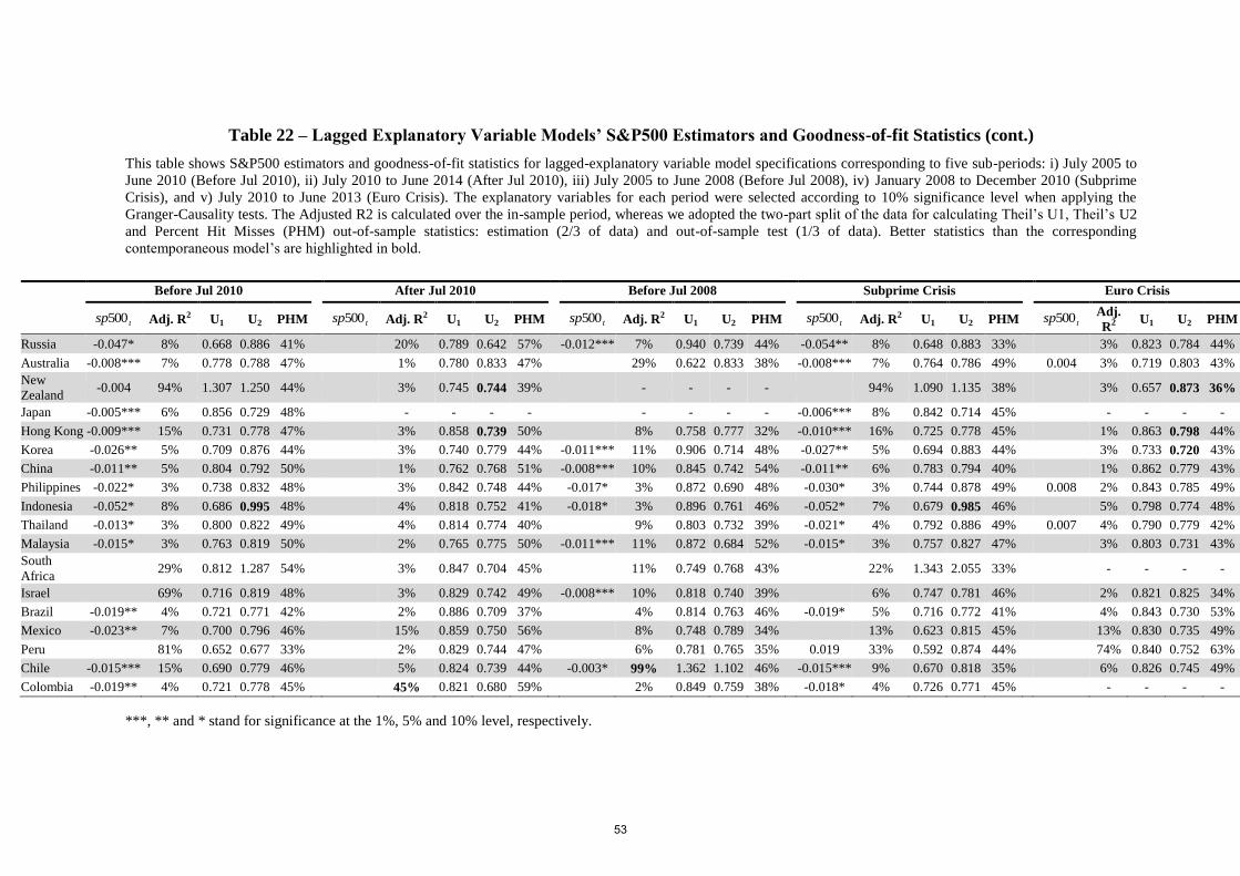
Table 22 – Lagged Explanatory Variable Models’ S&P500 Estimators and Goodness-of-fit Statistics (cont.)
This table shows S&P500 estimators and goodness-of-fit statistics for lagged-explanatory variable model specifications corresponding to five sub-periods: i) July 2005 to
June 2010 (Before Jul 2010), ii) July 2010 to June 2014 (After Jul 2010), iii) July 2005 to June 2008 (Before Jul 2008), iv) January 2008 to December 2010 (Subprime
Crisis), and v) July 2010 to June 2013 (Euro Crisis). The explanatory variables for each period were selected according to 10% significance level when applying the
Granger-Causality tests. The Adjusted R2 is calculated over the in-sample period, whereas we adopted the two-part split of the data for calculating Theil’s U1, Theil’s U2
and Percent Hit Misses (PHM) out-of-sample statistics: estimation (2/3 of data) and out-of-sample test (1/3 of data). Better statistics than the corresponding
contemporaneous model’s are highlighted in bold.
Before Jul 2010 After Jul 2010 Before Jul 2008 Subprime Crisis Euro Crisis
tsp500 Adj. R2 U1 U2 PHM tsp500 Adj. R2 U1 U2 PHM tsp500 Adj. R2 U1 U2 PHM tsp500 Adj. R2 U1 U2 PHM tsp500Adj.
R2 U1 U2 PHM
Russia -0.047* 8% 0.668 0.886 41% 20% 0.789 0.642 57% -0.012*** 7% 0.940 0.739 44% -0.054** 8% 0.648 0.883 33% 3% 0.823 0.784 44%
Australia -0.008*** 7% 0.778 0.788 47% 1% 0.780 0.833 47% 29% 0.622 0.833 38% -0.008*** 7% 0.764 0.786 49% 0.004 3% 0.719 0.803 43%
New
Zealand -0.004 94% 1.307 1.250 44% 3% 0.745 0.744 39% - - - - 94% 1.090 1.135 38% 3% 0.657 0.873 36%
Japan -0.005*** 6% 0.856 0.729 48% - - - - - - - - -0.006*** 8% 0.842 0.714 45% - - - -
Hong Kong -0.009*** 15% 0.731 0.778 47% 3% 0.858 0.739 50% 8% 0.758 0.777 32% -0.010*** 16% 0.725 0.778 45% 1% 0.863 0.798 44%
Korea -0.026** 5% 0.709 0.876 44% 3% 0.740 0.779 44% -0.011*** 11% 0.906 0.714 48% -0.027** 5% 0.694 0.883 44% 3% 0.733 0.720 43%
China -0.011** 5% 0.804 0.792 50% 1% 0.762 0.768 51% -0.008*** 10% 0.845 0.742 54% -0.011** 6% 0.783 0.794 40% 1% 0.862 0.779 43%
Philippines -0.022* 3% 0.738 0.832 48% 3% 0.842 0.748 44% -0.017* 3% 0.872 0.690 48% -0.030* 3% 0.744 0.878 49% 0.008 2% 0.843 0.785 49%
Indonesia -0.052* 8% 0.686 0.995 48% 4% 0.818 0.752 41% -0.018* 3% 0.896 0.761 46% -0.052* 7% 0.679 0.985 46% 5% 0.798 0.774 48%
Thailand -0.013* 3% 0.800 0.822 49% 4% 0.814 0.774 40% 9% 0.803 0.732 39% -0.021* 4% 0.792 0.886 49% 0.007 4% 0.790 0.779 42%
Malaysia -0.015* 3% 0.763 0.819 50% 2% 0.765 0.775 50% -0.011*** 11% 0.872 0.684 52% -0.015* 3% 0.757 0.827 47% 3% 0.803 0.731 43%
South
Africa 29% 0.812 1.287 54% 3% 0.847 0.704 45% 11% 0.749 0.768 43% 22% 1.343 2.055 33% - - - -
Israel 69% 0.716 0.819 48% 3% 0.829 0.742 49% -0.008*** 10% 0.818 0.740 39% 6% 0.747 0.781 46% 2% 0.821 0.825 34%
Brazil -0.019** 4% 0.721 0.771 42% 2% 0.886 0.709 37% 4% 0.814 0.763 46% -0.019* 5% 0.716 0.772 41% 4% 0.843 0.730 53%
Mexico -0.023** 7% 0.700 0.796 46% 15% 0.859 0.750 56% 8% 0.748 0.789 34% 13% 0.623 0.815 45% 13% 0.830 0.735 49%
Peru 81% 0.652 0.677 33% 2% 0.829 0.744 47% 6% 0.781 0.765 35% 0.019 33% 0.592 0.874 44% 74% 0.840 0.752 63%
Chile -0.015*** 15% 0.690 0.779 46% 5% 0.824 0.739 44% -0.003* 99% 1.362 1.102 46% -0.015*** 9% 0.670 0.818 35% 6% 0.826 0.745 49%
Colombia -0.019** 4% 0.721 0.778 45% 45% 0.821 0.680 59% 2% 0.849 0.759 38% -0.018* 4% 0.726 0.771 45% - - - -
***, ** and * stand for significance at the 1%, 5% and 10% level, respectively.
53