shtukas and the taylor expansion of...
TRANSCRIPT

Annals of Mathematics 186 (2017), 767–911https://doi.org/10.4007/annals.2017.186.3.2
Shtukas and the Taylor expansionof L-functions
By Zhiwei Yun and Wei Zhang
Abstract
We define the Heegner–Drinfeld cycle on the moduli stack of Drinfeld
Shtukas of rank two with r-modifications for an even integer r. We prove an
identity between (1) the r-th central derivative of the quadratic base change
L-function associated to an everywhere unramified cuspidal automorphic
representation π of PGL2, and (2) the self-intersection number of the π-
isotypic component of the Heegner–Drinfeld cycle. This identity can be
viewed as a function-field analog of the Waldspurger and Gross–Zagier
formula for higher derivatives of L-functions.
Contents
1. Introduction 768
Part 1. The analytic side 781
2. The relative trace formula 781
3. Geometric interpretation of orbital integrals 788
4. Analytic spectral decomposition 797
Part 2. The geometric side 807
5. Moduli spaces of Shtukas 807
6. Intersection number as a trace 821
7. Cohomological spectral decomposition 845
Part 3. The comparison 869
8. Comparison for most Hecke functions 869
9. Proof of the main theorems 874
Keywords: L-functions, Drinfeld Shtukas, Gross–Zagier formula, Waldspurger formula
AMS Classification: Primary: 11F67; Secondary: 14G35, 11F70, 14H60.
Research of Z.Yun partially supported by the Packard Foundation and the NSF grant
DMS-1302071/DMS-1736600. Research of W. Zhang partially supported by the NSF grants
DMS-1301848 and DMS-1601144, and a Sloan research fellowship.
c© 2017 Department of Mathematics, Princeton University.
767

768 ZHIWEI YUN and WEI ZHANG
Appendix A. Results from intersection theory 880
Appendix B. Super-positivity of L-values 901
Index 907
References 909
1. Introduction
In this paper we prove a formula for the arbitrary order central derivative
of a certain class of L-functions over a function field F = k(X) for a curve
X over a finite field k of characteristic p > 2. The L-function under consid-
eration is associated to a cuspidal automorphic representation of PGL2,F , or
rather, its base change to a quadratic field extension of F . The r-th central
derivative of our L-function is expressed in terms of the intersection number
of the “Heegner–Drinfeld cycle” on a moduli stack denoted by ShtrG in the
introduction, where G = PGL2. The moduli stack ShtrG is closely related to
the moduli stack of Drinfeld Shtukas of rank two with r-modifications. One
important feature of this stack is that it admits a natural fibration over the
r-fold self-product Xr of the curve X over Spec k
ShtrG // Xr.
The very existence of such moduli stacks presents a striking difference between
a function field and a number field. In the number field case, the analogous
spaces only exist (at least for the time being) when r ≤ 1. When r = 0, the
moduli stack Sht0G is the constant groupoid over k
(1.1) BunG(k) ' G(F )\(G(A)/K),
where A is the ring of adeles and K is a maximal compact open subgroup of
G(A). The double coset in the right-hand side of (1.1) remains meaningful for
a number field F (except that one cannot demand the archimedean component
of K to be open). When r = 1 the analogous space in the case F = Q is the
moduli stack of elliptic curves, which lives over SpecZ. From such perspectives,
our formula can be viewed as a simultaneous generalization (for function fields)
of the Waldspurger formula [26] (in the case of r = 0) and the Gross–Zagier
formula [11] (in the case of r = 1).
Another noteworthy feature of our work is that we need not restrict our-
selves to the leading coefficient in the Taylor expansion of the L-functions:
our formula is about the r-th Taylor coefficient of the L-function regardless
whether r is the central vanishing order or not. This leads us to speculate
that, contrary to the usual belief, central derivatives of arbitrary order of mo-
tivic L-functions (for instance, those associated to elliptic curves) should bear
some geometric meaning in the number field case. However, due to the lack

TAYLOR EXPANSION 769
of the analog of ShtrG for arbitrary r in the number field case, we could not
formulate a precise conjecture.
Finally we note that, in the current paper, we restrict ourselves to every-
where unramified cuspidal automorphic representations. One consequence is
that we only need to consider the even r case. Ramifications, particularly the
odd r case, will be considered in subsequent work.
Now we give more details of our main theorems.
1.1. Some notation. Throughout the paper, let k = Fq be a finite field of
characteristic p > 2. Let X be a geometrically connected smooth proper curve
over k. Let ν : X ′ → X be a finite etale cover of degree 2 such that X ′ is also
geometrically connected. Let σ ∈ Gal(X ′/X) be the nontrivial involution. Let
F = k(X) and F ′ = k(X ′) be their function fields. Let g and g′ be the genera
of X and X ′, then g′ = 2g − 1.
We denote the set of closed points (places) of X by |X|. For x ∈ |X|, let
Ox be the completed local ring of X at x and let Fx be its fraction field. Let
A =∏′x∈|X| Fx be the ring of adeles, and let O =
∏x∈|X|Ox be the ring of
integers inside A. Similar notation applies to X ′. Let
ηF ′/F : F×\A×/O× // ±1
be the character corresponding to the etale double cover X ′ via class field
theory.
Let G = PGL2. Let K =∏x∈|X|Kx where Kx = G(Ox). The (spherical)
Hecke algebra H is the Q-algebra of bi-K-invariant functions C∞c (G(A)//K,Q)
with the product given by convolution.
1.2. L-functions. Let A = C∞c (G(F )\G(A)/K,Q) be the space of ev-
erywhere unramified Q-valued automorphic functions for G. Then A is an
H -module. By an everywhere unramified cuspidal automorphic representa-
tion π of G(AF ) we mean an H -submodule Aπ ⊂ A that is irreducible over Q.
For every such π, EndH (Aπ) is a number field Eπ, which we call the co-
efficient field of π. Then by the commutativity of H , Aπ is a one-dimensional
Eπ-vector space. If we extend scalars to C, Aπ splits into one-dimensional
HC-modules Aπ ⊗Eπ ,ι C, one for each embedding ι : Eπ → C, and each
Aπ⊗Eπ ,ιC ⊂ AC is the unramified vectors of an everywhere unramified cuspidal
automorphic representation in the usual sense.
The standard (complete) L-function L(π, s) is a polynomial of degree
4(g−1) in q−s−1/2 with coefficients in the ring of integers OEπ . Let πF ′ be the
base change to F ′, and let L(πF ′ , s) be the standard L-function of πF ′ . This
L-function is a product of two L-functions associated to cuspidal automorphic
representations of G over F :
L(πF ′ , s) = L(π, s)L(π ⊗ ηF ′/F , s).

770 ZHIWEI YUN and WEI ZHANG
Therefore, L(πF ′ , s) is a polynomial of degree 8(g − 1) in q−s−1/2 with coeffi-
cients in Eπ. It satisfies a functional equation
L(πF ′ , s) = ε(πF ′ , s)L(πF ′ , 1− s),
where the epsilon factor takes a simple form
ε(πF ′ , s) = q−8(g−1)(s−1/2).
Let L(π,Ad, s) be the adjoint L-function of π. Denote
(1.2) L (πF ′ , s) = ε(πF ′ , s)−1/2 L(πF ′ , s)
L(π,Ad, 1),
where the the square root is understood as
ε(πF ′ , s)−1/2 := q4(g−1)(s−1/2).
Then we have a functional equation:
L (πF ′ , s) = L (πF ′ , 1− s).
Note that the constant factor L(π,Ad, 1) in L (πF ′ , s) does not affect the func-
tional equation, and it shows up only through the calculation of the Petersson
inner product of a spherical vector in π; see the proof of Theorem 4.5.
Consider the Taylor expansion at the central point s = 1/2:
L (πF ′ , s) =∑r≥0
L (r)(πF ′ , 1/2)(s− 1/2)r
r!,
i.e.,
L (r)(πF ′ , 1/2) =dr
dsr
∣∣∣∣s=0
Çε(πF ′ , s)
−1/2 L(πF ′ , s)
L(π,Ad, 1)
å.
If r is odd, by the functional equation we have
L (r)(πF ′ , 1/2) = 0.
Since L(π,Ad, 1) ∈ Eπ, we have L (πF ′ , s) ∈ Eπ[q−s−1/2, qs−1/2]. It follows
that
L (r)(πF ′ , 1/2) ∈ Eπ · (log q)r.
The main result of this paper is to relate each even degree Taylor coefficient to
the self-intersection numbers of a certain algebraic cycle on the moduli stack
of Shtukas. We give two formulations of our main results, one using certain
subquotient of the rational Chow group, and the other using `-adic cohomology.

TAYLOR EXPANSION 771
1.3. The Heegner–Drinfeld cycles. From now on, we let r be an even in-
teger. In Section 5.2, we will introduce moduli stack ShtrG of Drinfeld Shtukas
with r-modifications for the group G = PGL2. The stack ShtrG is a Deligne–
Mumford stack over Xr, and the natural morphism
πG : ShtrG // Xr
is smooth of relative dimension r, and locally of finite type.
Let T = (ResF ′/F Gm)/Gm be the nonsplit torus associated to the double
cover X ′ of X. In Section 5.4, we will introduce the moduli stack ShtµT of
T -Shtukas, depending on the choice of an r-tuple of signs µ ∈ ±r satisfying
certain balance conditions in Section 5.1.2. Then we have a similar map
πµT : ShtµT// X ′r,
which is a torsor under the finite Picard stack PicX′(k)/PicX(k). In particular,
ShtµT is a proper smooth Deligne–Mumford stack over Spec k.
There is a natural finite morphism of stacks over Xr
ShtµT// ShtrG .
It induces a finite morphism
θµ : ShtµT// Sht′rG := ShtrG ×Xr X ′r.
This defines a class in the Chow group
θµ∗ [ShtµT ] ∈ Chc,r(Sht′rG)Q.
Here Chc,r(−)Q means the Chow group of proper cycles of dimension r, ten-
sored over Q. See Section A.1 for details. In analogy to the classical Heegner
cycles [11], we will call θµ∗ [ShtµT ] the Heegner–Drinfeld cycle in our setting.
1.4. Main results : cycle-theoretic version. The Hecke algebra H acts on
the Chow group Chc,r(Sht′rG)Q as correspondences. Let W ⊂ Chc,r(Sht′rG)Q be
the sub H -module generated by the Heegner–Drinfeld cycle θµ∗ [ShtµT ]. There
is a bilinear and symmetric intersection pairing1
(1.3) 〈·, ·〉Sht′rG: W × W // Q.
Let W0 be the kernel of the pairing, i.e.,
W0 =z ∈ W
∣∣∣ (z, z′) = 0, for all z′ ∈ W.
1In this paper, the intersection pairing on the Chow groups will be denoted by 〈·, ·〉, and
other pairings (those on the quotient of the Chow groups, and the cup product pairing on
cohomology) will be denoted by (·, ·).

772 ZHIWEI YUN and WEI ZHANG
The pairing 〈·, ·〉Sht′rGthen induces a nondegenerate pairing on the quotient
W := W/W0
(·, ·) : W ×W // Q .(1.4)
The Hecke algebra H acts on W . For any ideal I ⊂H , let
W [I] =w ∈W
∣∣∣ I · w = 0.
Let π be an everywhere unramified cuspidal automorphic representation of G
with coefficient field Eπ, and let λπ : H → Eπ be the associated character,
whose kernel mπ is a maximal ideal of H . Let
Wπ = W [mπ] ⊂W
be the λπ-eigenspace of W . This is an Eπ-vector space. Let IEis ⊂ H be the
Eisenstein ideal as defined in Definition 4.1, and define
WEis = W [IEis].
Theorem 1.1. We have an orthogonal decomposition of H -modules
(1.5) W = WEis ⊕Ç⊕
π
Wπ
å,
where π runs over the finite set of everywhere unramified cuspidal automorphic
representation of G and Wπ is an Eπ-vector space of dimension at most one.
The proof will be given in Section 9.3.1. In fact one can also show thatWEis
is a free rank one module over Q[PicX(k)]ιPic (for notation see Section 4.1.2),
but we shall omit the proof of this fact.
The Q-bilinear pairing (·, ·) on Wπ can be lifted to an Eπ-bilinear sym-
metric pairing
(1.6) (·, ·)π : Wπ ×Wπ// Eπ,
where for w,w′ ∈Wπ, (w,w′)π is the unique element in Eπ such that TrEπ/Q(e·(w,w′)π) = (ew,w′).
We now present the cycle-theoretic version of our main result.
Theorem 1.2. Let π be an everywhere unramified cuspidal automorphic
representation of G with coefficient field Eπ . Let [ShtµT ]π ∈Wπ be the projection
of the image of θµ∗ [ShtµT ] ∈ W in W to the direct summand Wπ under the
decomposition (1.5). Then we have an equality in Eπ
1
2(log q)r|ωX |L (r) (πF ′ , 1/2) =
([ShtµT ]π, [ShtµT ]π
)π,
where ωX is the canonical divisor of X , and |ωX | = q− degωX .
The proof will be completed in Section 9.3.2.

TAYLOR EXPANSION 773
Remark 1.3. Assume that r = 0. Then our formula is equivalent to the
Waldspurger formula [26] for an everywhere unramified cuspidal automorphic
representation π. More precisely, for any nonzero φ ∈ πK , the Waldspurger
formula is the identity
1
2|ωX |L (πF ′ , 1/2) =
∣∣∣∫T (F )\T (A) φ(t) dt∣∣∣2
〈φ, φ〉Pet,
where 〈φ, φ〉Pet is the Petersson inner product (4.10), and the measure on G(A)
(resp. T (A)) is chosen such that vol(K) = 1 (resp. vol(T (O)) = 1).
Remark 1.4. Our Eπ-valued intersection paring is similar to the Neron–
Tate height pairing with coefficients in [27, §1.2.4].
1.5. Main results : cohomological version. Let ` be a prime number differ-
ent from p. Consider the middle degree cohomology with compact support
V ′Q` = H2rc ((Sht′rG)⊗k k,Q`)(r).
In the main body of the paper, we simply denote this by V ′. This vector space
is endowed with the cup product
(·, ·) : V ′Q` × V′Q`
// Q`.
Then for any maximal ideal m ⊂HQ` , we define the generalized eigenspace of
V ′Q` with respect to m by
V ′Q`,m = ∪i>0V′Q` [m
i].
We also define the Eisenstein part of V ′Q` by
V ′Q`,Eis = ∪i>0V′Q` [I
iEis].
We remark that in the cycle-theoretic version (cf. Section 1.4), the gener-
alized eigenspace coincides with the eigenspace because the space W is a cyclic
module over the Hecke algebra.
Theorem 1.5 (see Theorem 7.16 for a more precise statement). We have
an orthogonal decomposition of HQ`-modules
(1.7) V ′Q` = V ′Q`,Eis ⊕Ç⊕
m
V ′Q`,m
å,
where m runs over a finite set of maximal ideals of HQ` whose residue fields
Em := HQ`/m are finite extensions of Q`, and each V ′Q`,m is an HQ`-module
of finite dimension over Q` supported at the maximal ideal m.
The action of HQ` on V ′Q`,m factors through the completion ”HQ`,m with
residue field Em. Since Em is finite etale over Q`, and ”HQ`,m is a complete local
(hence henselian) Q`-algebra with residue field Em, Hensel’s lemma implies

774 ZHIWEI YUN and WEI ZHANG
that there is a unique section Em → ”HQ`,m. (The minimal polynomial of every
element h ∈ Em over Q` has a unique root h ∈ ”HQ`,m whose reduction is h.)
Hence each V ′Q`,m is also an Em-vector space in a canonical way. As in the case
of Wπ, using the Em-action on V ′Q`,m, the Q`-bilinear pairing on V ′Q`,m may be
lifted to an Em-bilinear symmetric pairing
(·, ·)m : V ′Q`,m × V′Q`,m
// Em.
Note that, unlike (1.5), in the decomposition (1.7) we cannot be sure
whether all m are automorphic; i.e., the homomorphism H → Em is the
character by which H acts on the unramified line of an irreducible automorphic
representation. However, for an everywhere unramified cuspidal automorphic
representation π of G with coefficient field Eπ, we may extend λπ : H → Eπto Q` to get
λπ ⊗Q` : HQ`// Eπ ⊗Q`
∼=∏λ|`Eπ,λ
where λ runs over places of Eπ above `. Let mπ,λ be the maximal ideal of HQ`obtained as the kernel of the λ-component of the above map HQ` → Eπ,λ.
To alleviate notation, we denote V ′Q`,mπ,λ simply by V ′π,λ and denote the
Eπ,λ-bilinear pairing (·, ·)mπ,λ on V ′π,λ by
(·, ·)π,λ : V ′π,λ × V ′π,λ // Eπ,λ.
We now present the cohomological version of our main result.
Theorem 1.6. Let π be an everywhere unramified cuspidal automorphic
representation of G with coefficient field Eπ . Let λ be a place of Eπ above `.
Let [ShtµT ]π,λ ∈ V ′π,λ be the projection of the cycle class cl(θµ∗ [ShtµT ]) ∈ V ′Q`to the direct summand V ′π,λ under the decomposition (1.7). Then we have an
equality in Eπ,λ
1
2(log q)r|ωX |L (r) (πF ′ , 1/2) =
([ShtµT ]π,λ, [ShtµT ]π,λ
)π,λ.
In particular, the right-hand side also lies in Eπ .
The proof will be completed in Section 9.2.
1.6. Two other results. We have the following positivity result. This may
be seen as an evidence of the Hodge standard conjecture (on the positivity of
intersection pairing) for a subquotient of the Chow group of middle-dimensional
cycles on Sht′rG.
Theorem 1.7. Let Wcusp be the orthogonal complement of WEis in W
(cf. (1.5)). Then the restriction to Wcusp of the intersection pairing (·, ·) in
(1.4) is positive definite.

TAYLOR EXPANSION 775
Proof. The assertion is equivalent to the positivity for the restriction to
Wπ of the intersection pairing for all π in (1.5). Fix such a π. Then the coeffi-
cient field Eπ is a totally real number field because the Hecke operators H act
on the positive definite inner product space A⊗QR (under the Petersson inner
product) by self-adjoint operators. For an embedding ι : Eπ → R, we define
Wπ,ι := Wπ ⊗Eπ ,ι R.Extending scalars from Eπ to R via ι, the pairing (1.6) induces an R-bilinear
symmetric pairing(·, ·)π,ι : Wπ,ι ×Wπ,ι
// R.It suffices to show that, for every embedding ι : Eπ → R, the pairing (·, ·)π,ι is
positive definite. The R-vector space Wπ,ι is at most one dimensional, with a
generator given by [ShtµT ]π,ι = [ShtµT ]π⊗1. The embedding ι gives an irreducible
cuspidal automorphic representation πι with R-coefficient. Then Theorem 1.2
implies that1
2(log q)r|ωX |L (r) (πι,F ′ , 1/2) =
([ShtµT ]π,ι, [ShtµT ]π,ι
)π,ι∈ R.
It is easy to see that L(πι,Ad, 1) > 0. By Theorem B.2, we have
L (r) (πι,F ′ , 1/2) ≥ 0.
It follows that ([ShtµT ]π,ι, [ShtµT ]π,ι
)π,ι≥ 0.
This completes the proof.
Another result is a “Kronecker limit formula” for function fields. Let
L(η, s) be the (complete) L-function associated to the Hecke character η.
Theorem 1.8. When r > 0 is even, we have
〈θµ∗ [ShtµT ], θµ∗ [ShtµT ]〉Sht′rG=
2r+2
(log q)rL(r)(η, 0).
The proof will be given in Section 9.1.1. For the case r = 0, see Re-
mark 9.3.
Remark 1.9. To obtain a similar formula for the odd order derivatives
L(r)(η, 0), we need moduli spaces analogous to ShtµT and Sht′rG for odd r. We
will return to this in future work.
1.7. Outline of the proof of the main theorems.
1.7.1. Basic strategy. The basic strategy is to compare two relative trace
formulae. A relative trace formula (abbreviated as RTF) is an equality between
a spectral expansion and an orbital integral expansion. We have two RTFs, an
“analytic” one for the L-functions, and a “geometric” one for the intersection
numbers, corresponding to the two sides of the desired equality in Theorem 1.6.

776 ZHIWEI YUN and WEI ZHANG
We may summarize the strategy of the proof into the following diagram:
(1.8)
Analytic:∑u∈P1(F )−1 Jr(u, f)
§2
∼Th 8.1 ⇒
Jr(f)§4
Th 9.2 ⇒
∑π Jr(π, f)
⇒Th 1.6
Geometric:∑u∈P1(F )−1 Ir(u, f)
§6Ir(f)
§7 ∑m Ir(m, f)
The vertical lines mean equalities after dividing the first row by (log q)r.
1.7.2. The analytic side. We start with the analytic RTF. To an f ∈ H(or more generally, C∞c (G(A))), one first associates an automorphic kernel
function Kf on G(A)×G(A) and then a regularized integral:
J(f, s) =
∫ reg
[A]×[A]Kf (h1, h2)|h1h2|sη(h2) dh1 dh2.
Here A is the diagonal torus ofG and [A] = A(F )\A(A). We refer to Section 2.2
for the definition of the weighted factors and the regularization. Informally, we
may view this integral as a weighted (naive) intersection number on the con-
stant groupoid BunG(k) (the moduli stack of Shtukas with r = 0 modifications)
between BunA(k) and its Hecke translation under f of BunA(k).
The resulting J(f, s) belongs to Q[q−s, qs]. For an f in the Eisenstein ideal
IEis (cf. Section 4.1), the spectral decomposition of J(f, s) takes a simple form:
it is the sum of
Jπ(f, s) =1
2|ωX |L (πF ′ , s+ 1/2)λπ(f),
where π runs over all everywhere unramified cuspidal automorphic represen-
tations π of G with Q`-coefficients (cf. Proposition 4.5). We define Jr(f) to be
the r-th derivative
Jr(f) :=
Åd
ds
ãr ∣∣∣∣s=0
J(f, s).
We point out that in the case of r = 0, the relative trace formula in
question was first introduced by Jacquet [12], in his reproof of Waldspurger’s
formula. In the case of r = 1, a variant was first considered in [30] (for number
fields).
1.7.3. The geometric side. Next we consider the geometric RTF. We con-
sider the Heegner–Drinfeld cycle θµ∗ [ShtµT ] and its translation by the Hecke
correspondence given by f ∈H , both being cycles on the ambient stack Sht′rG.
We define Ir(f) to be their intersection number
Ir(f) := 〈θµ∗ [ShtµT ], f ∗ θµ∗ [ShtµT ]〉Sht′rG∈ Q, f ∈H .

TAYLOR EXPANSION 777
To decompose this spectrally according to the Hecke action, we have two per-
spectives, one viewing the Heegner–Drinfeld cycle as an element in the Chow
group modulo numerical equivalence, the other considering the cycle class of
the Heegner–Drinfeld cycle in the `-adic cohomology. In either case, when f
is in a certain power of IEis, the spectral decomposition (Section 7 or Theo-
rem 1.5) of WQ`or V ′Q`
as an HQ`-module expresses Ir(f) as a sum of
Ir(m, f) =([ShtµT ]m, f ∗ [ShtµT ]m
),
where m runs over a finite set of maximal ideals of HQ`whose corresponding
generalized eigenspaces appear discretely in WQ`or V ′Q`
. We remark that
the method of the proof of the spectral decomposition in Theorem 1.5 can
potentially be applied to moduli of Shtukas for more general groups G, which
should lead to a better understanding of the cohomology of these moduli spaces.
We point out here that we use the same method as in [30] to set up the
geometric RTF, although in [30] only the case of r = 1 was considered. In the
case r = 0, Jacquet used an integration of kernel function to set up an RTF
for the T -period integral, which is equivalent to our geometric RTF because in
this case ShtµT and ShtrG become discrete stacks BunT (k) and BunG(k). Our
geometric formulation treats all values of r uniformly.
1.7.4. The key identity. In view of the spectral decompositions of both
Ir(f) and Jr(f), to prove the main Theorem 1.6 for all π simultaneously, it
suffices to establish the following key identity (cf. Theorem 9.2):
(1.9) Ir(f) = (log q)−rJr(f) ∈ Q for all f ∈H .
This key identity also allows us to deduce Theorem 1.1 on the spectral de-
composition of the space W of cycles from the spectral decomposition of Jr.Theorem 1.2 then follows easily from Theorem 1.6.
Since half of the paper is devoted to the proof of the key identity (1.9),
we comment on its proof in more detail. The spectral decompositions allow us
to reduce to proving (1.9) for sufficiently many functions f ∈ H , indexed by
effective divisors on X with large degree compared to the genus of X (cf. The-
orem 8.1). Most of the algebro-geometric part of this paper is devoted to the
proof of the key identity (1.9) for those Hecke functions.
In Section 3, we interpret the orbital integral expansion of Jr(f) (the upper
left sum in (1.8)) as a certain weighted counting of effective divisors on the
curve X. The geometric ideas used in the part are close to those in the proof
of various fundamental lemmas by Ngo [20] and by the first-named author [29],
although the situation is much simpler in the current paper. In Section 6, we
interpret the intersection number Ir(f) as the trace of a correspondence acting
on the cohomology of a certain variety. This section involves new geometric

778 ZHIWEI YUN and WEI ZHANG
ideas that did not appear in the treatment of the fundamental lemma type
problems. This is also the most technical part of the paper, making use of the
general machinery on intersection theory reviewed or developed in Appendix A.
After the preparations in Sections 3 and 6, our situation can be summa-
rized as follows. For an integer d ≥ 0, we have fibrations
fN : Nd =⊔d
Nd −→ Ad, fM :Md −→ Ad,
where d runs over all quadruples (d11, d12, d21, d22) ∈ Z4≥0 such that d11 +d22 =
d = d12 + d21. We need to show that the direct image complexes RfM,∗Q`
and RfN ,∗Ld are isomorphic to each other, where Ld is a local system of
rank one coming from the double cover X ′/X. When d is sufficiently large,
we show that both complexes are shifted perverse sheaves, and are obtained
by middle extension from a dense open subset of Ad over which both can be
explicitly calculated (cf. Propositions 8.2 and 8.5). The isomorphism between
the two complexes over the entire base Ad then follows by the functoriality
of the middle extension. The strategy used here is the perverse continuation
principle coined by Ngo, which has already played a key role in all known
geometric proofs of fundamental lemmas; see [20] and [29].
Remark 1.10. One feature of our proof of the key identity (1.9) is that it
is entirely global, in the sense that we do not reduce to the comparison of local
orbital integral identities, as opposed to what one usually does when comparing
two trace formulae. Therefore, our proof is different from Jacquet’s in the case
r = 0 in that his proof is essentially local. (This is inevitable because he also
considers the number field case.)
Another remark is that our proof of (1.9) in fact gives a term-by-term
identity of the orbital expansion of both Jr(f) and Ir(f), as indicated in the
left column of (1.8), although this is not logically needed for our main results.
However, such more refined identities (for more general G) will be needed in
the proof of the arithmetic fundamental lemma for function fields, a project to
be completed in the near future [28].
1.8. A guide for readers. Since this paper uses a mixture of tools from
automorphic representation theory, algebraic geometry and sheaf theory, we
think it might help orient the readers by providing a brief summary of the
contents and the background knowledge required for each section. We give the
“Leitfaden” in Table 1.
Section 2 sets up the relative trace formula following Jacquet’s approach
[12] to the Waldspurger formula. This section is purely representation-theo-
retic.
Section 3 gives a geometric interpretation of the orbital integrals involved
in the relative trace formula introduced in Section 2. We express these orbital

TAYLOR EXPANSION 779
Section 2
zz
Section 5
$$
Section 4
$$
Section 3
$$
Section 6
zz
Section 7
zz
Section 8
Section 9
Table 1.
integrals as the trace of Frobenius on the cohomology of certain varieties, in
the similar spirit of the proof of various fundamental lemmas ([20], [29]). This
section involves both orbital integrals and some algebraic geometry but not
yet perverse sheaves.
Section 4 relates the spectral side of the relative trace formula in Sec-
tion 2 to automorphic L-functions. Again this section is purely representation-
theoretic.
Section 5 introduces the geometric players in our main theorem: moduli
stacks ShtrG of Drinfeld Shtukas, and Heegner–Drinfeld cycles on them. We
give self-contained definitions of these moduli stacks, so no prior knowledge
of Shtukas is assumed, although some experience with the moduli stack of
bundles will help.
Section 6 is the technical heart of the paper, aiming to prove Theorem 6.5.
The proof involves studying several auxiliary moduli stacks and uses heavily the
intersection-theoretic tools reviewed and developed in Appendix A. The first-
time readers may skip the proof and only read the statement of Theorem 6.5.
Section 7 gives a decomposition of the cohomology of ShtrG under the
action of the Hecke algebra, generalizing the classical spectral decomposition
for the space automorphic forms. The idea is to remove the analytic ingredi-
ents from the classical treatment of spectral decomposition and to use solely
commutative algebra. (In particular, we crucially use the Eisenstein ideal in-
troduced in Section 4.) For first-time readers, we suggest read Section 7.1,
then jump directly to Definition 7.12 and continue from there. What he/she
will miss in doing this is the study of the geometry of ShtrG near infinity (horo-
cycles), which requires some familiarity with the moduli stack of bundles, and
the formalism of `-adic sheaves.

780 ZHIWEI YUN and WEI ZHANG
Section 8 combines the geometric formula for orbital integrals established
in Section 3 and the trace formula for the intersection numbers established in
Section 6 to prove the key identity (1.9) for most Hecke functions. The proofs
in this section involve perverse sheaves.
Section 9 finishes the proofs of our main results. Assuming results from
the previous sections, most arguments in this section only involve commutative
algebra.
Both appendices can be read independently of the rest of the paper. Ap-
pendix A reviews the intersection theory on algebraic stacks following Kresch
[14], with two new results that are used in Section 6 for the calculation of the
intersection number of Heegner–Drinfeld cycles. The first result, called the
Octahedron Lemma (Theorem A.10), is an elaborated version of the following
simple principle: in calculating the intersection product of several cycles, one
can combine terms and change the orders arbitrarily. The second result is a
Lefschetz trace formula for the intersection of a correspondence with the graph
of the Frobenius map, building on results of Varshavsky [24].
Appendix B proves a positivity result for central derivatives of automor-
phic L-functions, assuming the generalized Riemann hypothesis in the case
of number fields. The main body of the paper only considers L-functions for
function fields, for which the positivity result can be proved in an elementary
way (see Remark B.4).
1.9. Further notation.
1.9.1. Function field notation. For x ∈ |X|, let $x be a uniformizer of Ox,
kx be the residue field of x, dx = [kx : k], and qx = #kx = qdx . The valuation
map is a homomorphism
val : A× // Z
such that val($x) = dx. The normalized absolute value on A× is defined as
| · | : A× // Q×>0 ⊂ R×
a // q−val(a).
Denote the kernel of the absolute value by
A1 = Ker(| · |).
We have the global and local zeta function
ζF (s) =∏x∈|X|
ζx(s), ζx(s) =1
1− q−sx.
Denote by Div(X) ∼= A×/O× the group of divisors on X.

TAYLOR EXPANSION 781
1.9.2. Group-theoretic notation. Let G be an algebraic group over k. We
will view it as an algebraic group over F by extension of scalars. We will
abbreviate [G] = G(F )\G(A). Unless otherwise stated, the Haar measure on
the group G(A) will be chosen such that the natural maximal compact open
subgroup G(O) has volume equal to one. For example, the measure on A×,
resp. G(A) is such that vol (O×) = 1, resp. vol(K) = 1.
1.9.3. Algebro-geometric notation. In the main body of the paper, all geo-
metric objects are algebraic stacks over the finite field k = Fq. For such a
stack S, let FrS : S → S be the absolute q-Frobenius endomorphism that
raises functions to their q-th powers.
For an algebraic stack S over k, we write H∗(S ⊗k k) (resp. H∗c(S ⊗k k))
for the etale cohomology (resp. etale cohomology with compact support) of
the base change S ⊗k k with Q`-coefficients. The `-adic homology H∗(S ⊗k k)
and Borel-Moore homology HBM∗ (S ⊗k k) are defined as the graded duals of
H∗(S ⊗k k) and H∗c(S ⊗k k) respectively. We use Dbc(S) to denote the derived
category of Q`-complexes for the etale topology of S, as defined in [17]. We
use DS to denote the dualizing complex of S with Q`-coefficients.
Acknowledgement. We thank Akshay Venkatesh for a key conversation
that inspired our use of the Eisenstein ideal, and Dorian Goldfeld and Peter
Sarnak for their help on Appendix B. We thank Benedict Gross for his com-
ments, Michael Rapoport for communicating to us comments from the partic-
ipants of ARGOS in Bonn, and Shouwu Zhang for carefully reading the first
draft of the paper and providing many useful suggestions. We thank the Math-
ematisches Forschungsinstitut Oberwolfach to host the Arbeitsgemeinschaft in
April 2017 devoted to this paper, and we thank the participants, especially
Jochen Heinloth and Yakov Varshavsky, for their valuable feedbacks.
Part 1. The analytic side
2. The relative trace formula
In this section we set up the relative trace formula following Jacquet’s
approach [12] to the Waldspurger formula.
2.1. Orbits. In this subsection F is allowed to be an arbitrary field. Let
F ′ be a semisimple quadratic F -algebra; i.e., it is either the split algebra F ⊕For a quadratic field extension of F . Denote by Nm : F ′ → F the norm map.
Denote G = PGL2,F and A the subgroup of diagonal matrices in G. We
consider the action of A×A on G where (h1, h2) ∈ A×A acts by (h1, h2)g =

782 ZHIWEI YUN and WEI ZHANG
h−11 gh2. We define an A×A-invariant morphism:
inv : G // P1F − 1
γ // bcad ,
(2.1)
where[a bc d
]∈ GL2 is a lifting of γ. We say that γ ∈ G is A × A-regular
semisimple if
inv(γ) ∈ P1F − 0, 1,∞,
or equivalently all a, b, c, d are invertible in terms of the lifting of γ. Let Grs
be the open subscheme of A × A-regular semisimple locus. A section of the
restriction of the morphism inv to Grs is given by
γ : P1F − 0, 1,∞ // G
u // γ(u) =
ñ1 u
1 1
ô.
(2.2)
We consider the induced map on the F -points inv : G(F )→ P1(F )− 1and the action of A(F )×A(F ) on G(F ). Denote by
Ors(G) = A(F )\Grs(F )/A(F )
the set of orbits in Grs(F ) under the action of A(F )×A(F ). They will be called
the regular semisimple orbits. It is easy to see that the map inv : Grs(F ) →P1(F )− 0, 1,∞ induces a bijection
inv : Ors(G) −→ P1(F )− 0, 1,∞.
A convenient set of representative of Ors(G) is given by
Ors(G) '®γ(u) =
ñ1 u
1 1
ô ∣∣∣∣∣ u ∈ P1(F )− 0, 1,∞´.
There are six nonregular-semisimple orbits in G(F ), represented respectively
by
1 =
ñ1
1
ô, n+ =
ñ1 1
1
ô, n− =
ñ1
1 1
ô,
w =
ñ1
1
ô, wn+ =
ñ1
1 1
ô, wn− =
ñ1 1
1
ô,
where the first three (the last three, resp.) have inv = 0 (∞, resp.)

TAYLOR EXPANSION 783
2.2. Jacquet’s RTF. Now we return to the setting of the introduction. In
particular, we have η = ηF ′/F . In [12] Jacquet constructs an RTF to study the
central value of L-functions of the same type as ours (mainly in the number
field case). Here we modify his RTF to study higher derivatives.
For f ∈ C∞c (G(A)), we consider the automorphic kernel function
Kf (g1, g2) =∑
γ∈G(F )
f(g−11 γg2), g1, g2 ∈ G(A).(2.3)
We will define a distribution, given by a regularized integral
J(f, s) =
∫ reg
[A]×[A]Kf (h1, h2)|h1h2|sη(h2) dh1 dh2.
Here we recall that [A] = A(F )\A(A), and for h = [ a d ] ∈ A(A), for simplicity
we write ∣∣∣h∣∣∣ =∣∣∣a/d∣∣∣, η(h) = η(a/d).
The integral is not always convergent but can be regularized in a way analogous
to [12]. For an integer n, consider the “annulus”
A×n :=
®x ∈ A×
∣∣∣∣∣ val(x) = n
´.
This is a torsor under the group A1 = A×0 . Let A(A)n be the subset of A(A)
defined by
A(A)n =
®ña
d
ô∈ A(A)
∣∣∣∣∣ a/d ∈ A×n
´.
Then we define, for (n1, n2) ∈ Z2,
Jn1,n2(f, s) =
∫[A]n1×[A]n2
Kf (h1, h2)|h1h2|sη(h2) dh1 dh2.(2.4)
The integral (2.4) is clearly absolutely convergent and equal to a Laurent poly-
nomial in qs.
Proposition 2.1. The integral Jn1,n2(f, s) vanishes when |n1| + |n2| is
sufficiently large.
Granting this proposition, we then define
J(f, s) :=∑
(n1,n2)∈Z2
Jn1,n2(f, s).(2.5)
This is a Laurent polynomial in qs.
The proof of Proposition 2.1 will occupy Sections 2.3–2.5.

784 ZHIWEI YUN and WEI ZHANG
2.3. A finiteness lemma. For an (A×A)(F )-orbit of γ, we define
Kf,γ(h1, h2) =∑
δ∈A(F )γA(F )
f(h−11 δh2), h1, h2 ∈ A(A).(2.6)
Then we have
Kf (h1, h2) =∑
γ∈A(F )\G(F )/A(F )
Kf,γ(h1, h2).(2.7)
Lemma 2.2. The sum in (2.7) has only finitely many nonzero terms.
Proof. Denote by G(F )u the fiber of u under the (surjective) map (2.1)
inv : G(F ) −→ P1(F )− 1.
We then have a decomposition of G(F ) as a disjoint union
G(F ) =∐
u∈P1(F )−1G(F )u.
There is exactly one (three, resp.) (A × A)(F )-orbit in G(F )a when u ∈P1(F ) − 0, 1,∞ (when u ∈ 0,∞, resp.). It suffices to show that for all
but finitely many u ∈ P1(F ) − 0, 1,∞, the kernel function Kf,γ(u)(h1, h2)
vanishes identically on A(A)×A(A).
Consider the map
τ :=inv
1− inv: G(A) −→ A.
The map τ is continuous and takes constant values on A(A) × A(A)-orbits.
For Kf,γ(u)(h1, h2) to be nonzero, the invariant τ(γ(u)) = u1−u must be in the
image of supp(f), the support of the function f . Since supp(f) is compact, so
is its image under τ . On the other hand, the invariant τ(γ(u)) = u1−u belongs
to F . Since the intersection of a compact set supp(f) with a discrete set F
in A must have finite cardinality, the kernel function Kf,γ(u)(h1, h2) is nonzero
for only finitely many u.
For γ ∈ A(F )\G(F )/A(F ), we define
Jn1,n2(γ, f, s) =
∫[A]n1×[A]n2
Kf,γ(h1, h2)|h1h2|sη(h2) dh1 dh2.(2.8)
Then we have
Jn1,n2(f, s) =∑
γ∈A(F )\G(F )/A(F )
Jn1,n2(γ, f, s).
By the previous lemma, the above sum has only finitely many nonzero
terms. Therefore, to show Proposition 2.1, it suffices to show
Proposition 2.3. For any γ ∈ G(F ), the integral Jn1,n2(γ, f, s) vanishes
when |n1|+ |n2| is sufficiently large.
TAYLOR EXPANSION 785
Granting this proposition, we may define the (weighted) orbital integral
J(γ, f, s) :=∑
(n1,n2)∈Z2
Jn1,n2(γ, f, s).(2.9)
To show Proposition 2.3, we distinguish two cases according to whether γ is
regular semisimple.
2.4. Proof of Proposition 2.3: regular semisimple orbits. For u ∈ P1(F )−0, 1,∞, the fiber G(F )u = inv−1(u) is a single A(F ) × A(F )-orbit of γ(u),
and the stabilizer of γ(u) is trivial. We may rewrite (2.8) as
Jn1,n2(γ(u), f, s) =
∫A(A)n1×A(A)n2
f(h−11 γ(u)h2)|h1h2|sη(h2) dh1 dh2.(2.10)
For the regular semisimple γ = γ(u), the map
ιγ : (A×A)(A) −→ G(A)
(h1, h2) 7−→ h−11 γh2
is a closed embedding. It follows that the function f ιγ has compact support,
hence belongs to C∞c ((A×A)(A)). Therefore, the integrand in (2.10) vanishes
when |n1|+ |n2| 0 (depending on f and γ(u)).
2.5. Proof of Proposition 2.3: nonregular-semisimple orbits. Let u∈0,∞.We only consider the case u = 0 since the other case is completely analogous.
There are three orbit representatives 1, n+, n−.It is easy to see that for γ = 1, we have for all (n1, n2) ∈ Z2,
Jn1,n2(γ, f, s) = 0,
because η|A1 is a nontrivial character.
Now we consider the case γ = n+; the remaining case γ = n− is similar.
Define a function
φ(x, y) = f
Çñx y
1
ôå, (x, y) ∈ A× × A.(2.11)
Then we have φ ∈ C∞c (A× × A). The integral Jn1,n2(n+, f, s) is given by∫A×n1×A
×n2
φÄx−1y, x−1
äη(y)|xy|s d×x d×y,(2.12)
where we use the multiplicative measure d×x on A×. We substitute y by xy,
and then x by x−1:∫Z(n1,n2)
φ (y, x) η(xy)|x|−2s|y|s d×x d×y,
where
Z(n1, n2) =¶
(x, y) | x ∈ A(A)−n1 , x−1y ∈ A(A)n2
©.

786 ZHIWEI YUN and WEI ZHANG
Since C∞c (A× × A) ' C∞c (A×) ⊗ C∞c (A), we may reduce to the case
φ(x, y) = φ1(x)φ2(y) where φ1 ∈ C∞c (A×), φ2 ∈ C∞c (A). Moreover, by writing
φ1 as a finite linear combination, each supported on a single A×n , we may even
assume that supp(φ1) is contained in A×n for some n ∈ Z. The last integral is
equal toÇ∫A×n
φ1 (y) η(y)|y|s d×yå(∫
A×−n1∩A×−n2+n
φ2 (x) η(x)|x|−2s d×x
).
Finally we recall that, from Tate’s thesis, for any ϕ ∈ C∞c (A), the integral
on an annulus ∫A×n
ϕ (x) η(x)|x|2s d×x
vanishes when |n| 0. We briefly recall how this is proved. It is clear if
n 0. Now assume that n 0. We rewrite the integral as∫F×\A×n
∑α∈F×
ϕ (αx) η(x)|x|2s d×x.
The Fourier transform of ϕ, denoted by ϕ, still lies in C∞c (A). By the Poisson
summation formula, we have∑α∈F×
ϕ(αx) = −ϕ(0) + |x|−1ϕ(0) + |x|−1∑α∈F×
ϕ(α/x).(2.13)
By the boundedness of the support of ϕ, the sum over F× on the right-hand
side vanishes when val(x) = n 0. Finally we note that the the integral of
the remaining two terms on the right-hand side of (2.13) vanishes because η is
nontrivial on F×\A1.
This completes the proof of Propositions 2.3 and 2.1.
2.6. The distribution J. Now J(f, s) is a Laurent polynomial in qs. Con-
sider the r-th derivative
Jr(f) :=
Åd
ds
ãr ∣∣∣∣s=0
J(f, s).
For γ ∈ A(F )\G(F )/A(F ), we define
Jr(γ, f) :=
Åd
ds
ãr ∣∣∣∣s=0
J(γ, f, s).
We then have expansions (cf. (2.5))
J(f, s) =∑
γ∈A(F )\G(F )/A(F )
J(γ, f, s),
and (cf. (2.9))
Jr(f) =∑
γ∈A(F )\G(F )/A(F )
Jr(γ, f).(2.14)

TAYLOR EXPANSION 787
We define
J(u, f, s) =∑
γ∈A(F )\G(F )u/A(F )
J(γ, f, s), u ∈ P1(F )− 1(2.15)
and
Jr(u, f) =∑
γ∈A(F )\G(F )u/A(F )
Jr(γ, f), u ∈ P1(F )− 1.(2.16)
Then we have a slightly coarser decomposition than (2.14):
Jr(f) =∑
u∈P1(F )−1Jr(u, f).(2.17)
2.7. A special test function f = 1K .
Proposition 2.4. For the test function
f = 1K ,
we have
J(u,1K , s) =
L(η, 2s) + L(η,−2s) if u ∈ 0,∞,1 if u ∈ k − 0, 1,0 otherwise.
(2.18)
Proof. We first consider the case u ∈ P1(F ) − 0, 1,∞. In this case, we
have
J(u,1K , s) =
∫A××A×
1K
Çñx−1 0
0 1
ô ñ1 u
1 1
ô ñy 0
0 1
ôå|xy|sη(y) d×x d×y
=∑
x,y∈A×/O×1K
Çñx−1y x−1u
y 1
ôå|xy|sη(y).
The integrand is nonzero if and only if g =îx−1y x−1uy 1
ó∈ K. This is equivalent
to the condition that g2ij/ det(g) ∈ O, where gij1≤i,j≤2 are the entries of g.
We have det(g) = x−1y(1− u), therefore, g ∈ K is equivalent to
(2.19)x−1y(1− u)−1 ∈ O, x−1y−1u2(1− u)−1 ∈ O,
xy(1− u)−1 ∈ O, and xy−1(1− u)−1 ∈ O.
Multiplying the first and last conditions we get (1 − u)−1 ∈ O. Therefore,
1− u ∈ F× must be a constant function, i.e., u ∈ k − 0, 1. This shows that
J(u,1K , s) = 0 when u ∈ F − k.
When u ∈ k − 0, 1, the conditions (2.19) become
x−1y ∈ O, x−1y−1 ∈ O, xy ∈ O, and xy−1 ∈ O.
788 ZHIWEI YUN and WEI ZHANG
These together imply that x, y ∈ O×. Therefore, the integrand is nonzero only
when both x and y are in the unit coset of A×/O×, and the integrand is equal
to 1 when this happens. This proves J(u,1K , s) = 1 when u ∈ k − 0, 1.Next we consider the case u = 0. For f = 1K and γ = n+, in (2.11) we
have φ = φ1 ⊗ φ2, where
φ1 = 1O× , φ2 = 1O.
Therefore, we have
J(n+,1K , s) =
∫A×
φ2(x)η(x)|x|−2s d×x = L(η,−2s).
Similarly, we have
J(n−,1K , s) = L(η, 2s).
This proves the equality (2.18) for u = 0. The case for u =∞ is analogous.
Corollary 2.5. We have
Jr(1K) =
4L(η, 0) + q − 2 = 4
# JacX′ (k)# JacX(k) + q − 2 r = 0,
2r+2Ädds
är ∣∣∣∣s=0
L(η, s) r > 0 even,
0 r > 0 odd.
3. Geometric interpretation of orbital integrals
In this section, we will give a geometric interpretation of the orbital inte-
grals J(γ, f, s) (cf. (2.9)) as a certain weighted counting of effective divisors on
the curve X, when f is in the unramified Hecke algebra.
3.1. A basis for the Hecke algebra. Let x ∈ |X|. In the caseG = PGL2, the
local unramified Hecke algebra Hx is the polynomial algebra Q[hx], where hx is
the characteristic function of the G(Ox)-double coset of[$x 00 1
], and $x ∈ Ox
is a uniformizer. For each integer n ≥ 0, consider the set Mat2(Ox)vx(det)=n
of matrices A ∈ Mat2(Ox) such that vx(det(A)) = n. Let Mx,n be the image
of Mat2(Ox)vx(det)=n in G(Fx). Then Mx,n is a union of G(Ox)-double cosets.
We define hnx to be the characteristic function
(3.1) hnx = 1Mx,n .
Then hnxn≥0 is a Q-basis for Hx.
Now consider the global unramified Hecke algebra H = ⊗x∈|X|Hx, which
is a polynomial ring over Q with infinitely generators hx. For each effective
divisor D =∑x∈|X| nx · x, we can define an element hD ∈H using
(3.2) hD = ⊗x∈|X|hnxx,
where hnxx is defined in (3.1). It is easy to see that the set hD|D effective
divisor on X is a Q-basis for H .

TAYLOR EXPANSION 789
The goal of the next few subsections is to give a geometric interpretation
of the orbital integral J(γ, hD, s). We begin by defining certain moduli spaces.
3.2. Global moduli space for orbital integrals.
3.2.1. For d ∈ Z, we consider the Picard stack PicdX of lines bundles over
X of degree d. Note that PicdX is a Gm-gerbe over its coarse moduli space.
Let “Xd → PicdX be the universal family of sections of line bundles; i.e., an
S-point of “Xd is a pair (L, s), where L is a line bundle over X × S such that
degL|X×t = d for all geometric points t of S, and s ∈ H0(X × S,L).
When d < 0, “Xd∼= PicdX since all global sections of all line bundles
L ∈ PicdX vanish. When d ≥ 0, let Xd = Xd//Sd be the d-th symmetric power
of X. Then there is an open embedding Xd → “Xd as the open locus of nonzero
sections, with complement isomorphic to PicdX .
For d1, d2 ∈ Z, we have a morphism‘addd1,d2 : “Xd1 × “Xd2 −→ “Xd1+d2
sending ((L1, s1), (L2, s2)) to (L1 ⊗ L2, s1 ⊗ s2). The restriction of ‘addd1,d2 to
the open subset Xd1 × Xd2 becomes the addition map for divisors addd1,d2 :
Xd1 ×Xd2 → Xd1+d2 .
3.2.2. The moduli space Nd. Let d ≥ 0 be an integer. Let Σd be the set
of quadruple of nonnegative integers d = (dij)i,j∈1,2 satisfying d11 + d22 =
d12 + d21 = d.
For d∈Σd, we consider the moduli functor Nd classifying (K1,K2,K′1,K′2,ϕ)
where
• Ki,K′i ∈ PicX with degK′i − degKj = dij .
• ϕ : K1 ⊕K2 → K′1 ⊕K′2 is an OX -linear map. We express it as a matrix
ϕ =
ñϕ11 ϕ12
ϕ21 ϕ22
ô,
where ϕij : Kj → K′i.• If d11 < d22, then ϕ11 6= 0 otherwise ϕ22 6= 0. If d12 < d21, then ϕ12 6= 0
otherwise ϕ21 6= 0. Moreover, at most one of the four maps ϕij , i, j ∈ 1, 2can be zero.
The Picard stack PicX acts on Nd by tensoring each Ki and K′j with the same
line bundle. Let Nd be the quotient stack Nd/PicX , which will turn out to be
representable by a scheme over k. We remark that the artificial-looking last
condition in the definition of Nd is to guarantee that Nd is separated.
3.2.3. The base Ad. Let Ad be the moduli stack of triples (∆, a, b), where
∆ ∈ PicdX and a and b are sections of ∆ with the open condition that a and b

790 ZHIWEI YUN and WEI ZHANG
are not simultaneously zero. Then we have an isomorphism
(3.3) Ad ∼= “Xd ×PicdX“Xd − Zd,
where Zd ∼= PicdX is the image of the diagonal zero sections (0, 0) : PicdX →“Xd ×PicdX“Xd.
We claim that Ad is a scheme. In fact, A is covered by two opens V =“Xd ×PicdXXd and V ′ = Xd ×PicdX
“Xd. Both V and V ′ are schemes because the
map “Xd → PicdX is schematic.
We have a map
δ : Ad −→ “Xd
given by (∆, a, b) 7→ (∆, a− b).
3.2.4. The open part A♥d . Later we will consider the open subscheme
A♥d ⊂ Ad defined by the condition a 6= b, i.e., the preimage of Xd under
the map δ : Ad → “Xd.
3.2.5. To a point (K1,K2,K′1,K′2, ϕ) ∈ Nd we attach the following maps:
• a := ϕ11 ⊗ ϕ22 : K1 ⊗K2 → K′1 ⊗K′2;
• b := ϕ12 ⊗ ϕ21 : K1 ⊗K2 → K′2 ⊗K′1 ∼= K′1 ⊗K′2.
Both a and b can be viewed as sections of the line bundle ∆ = K′1 ⊗ K′2 ⊗K−1
1 ⊗ K−12 ∈ PicdX . Clearly this assignment (K1,K2,K′1,K′2, ϕ) 7→ (∆, a, b) is
invariant under the action of PicX on Nd. Therefore, we get a map
fNd : Nd −→ Ad.
The composition δ fNd : Nd → “Xd takes (K1,K2,K′1,K′2, ϕ) to det(ϕ) as a
section of ∆ = K′1 ⊗K′2 ⊗K−11 ⊗K
−12 .
3.2.6. Geometry of Nd. Fix d = (dij) ∈ Σd. For i, j ∈ 1, 2, we have
a morphism ij : Nd → “Xdij sending (K1, . . . ,K′2, ϕ) to the section ϕij of
the line bundle Lij := K′i ⊗ K−1j ∈ Pic
dijX . We have canonical isomorphisms
L11⊗L22∼= L12⊗L21
∼= ∆ = K′1⊗K′2⊗K−11 ⊗K
−12 . Thus we get a morphism
d = (ij)i,j : Nd−→ (“Xd11 × “Xd22)×PicdX(“Xd12 × “Xd21).(3.4)
Here the fiber product on the right side is formed using the maps “Xd11× “Xd22 →Picd11X ×Picd22X
⊗−→ PicdX and “Xd12 × “Xd21 → Picd12X ×Picd21X⊗−→ PicdX .
Proposition 3.1. Let d ∈ Σd.
(1) The morphism d is an open embedding, and Nd is a geometrically con-
nected scheme over k.
(2) If d ≥ 2g′− 1 = 4g− 3, then Nd is smooth over k of dimension 2d− g+ 1.

TAYLOR EXPANSION 791
(3) We have a commutative diagram
Nd d
//
fNd
(“Xd11 × “Xd22)×PicdX(“Xd12 × “Xd21)”addd11,d22×”addd12,d21
Ad
// “Xd ×PicdX“Xd.
(3.5)
Moreover, the map fNd is proper.
Proof. (1) We abbreviate PicdX by P d. Let Zd ⊂ (“Xd11 × “Xd22) ×PicdX
(“Xd12 × “Xd21) be the closed substack consisting of ((Lij , sij) ∈ “Xdij )1≤i,j≤2
such that
• either two of sij1≤i,j≤2 are zero,
• or s11 = 0 if d11 < d22,
• or s22 = 0 if d11 ≥ d22,
• or s12 = 0 if d12 < d21,
• or s21 = 0 if d12 ≥ d21.
By the definition of Nd, we have a Cartesian diagram
Ndd//
λ
(“Xd11 × “Xd22)×P d (“Xd12 × “Xd21)− Zd
P d11−d12 × P d11 × P d21ρ
// (P d11 × P d22)×P d (P d12 × P d21).
Here λ sends (K1, . . . ,K′2, ϕ) to (X2 = K2 ⊗ K−11 ,X ′1 = K′1 ⊗ K−1
1 ,X ′2 =
K′2 ⊗ K−11 ), and ρ sends (X2,X ′1,X ′2) to (X ′1,X ′2 ⊗ X−1
2 ,X ′1 ⊗ X−12 ,X ′2). Note
that ρ is an isomorphism. Therefore, d is an isomorphism. Since the geo-
metric fibers of λ are connected, and P d11−d12 × P d11 × P d21 is geometrically
connected, so is Nd.The stack Nd is covered by four open substacks Uij , i, j ∈ 1, 2, where Uij
is the locus where only ϕij is allow to be zero. Each Uij is a scheme over k. In
fact, for example, U11 is an open substack of (“Xd11 ×Xd22)×P d (Xd12 ×Xd21),
and the latter is a scheme since the morphism “Xd11 → P d11 is schematic.
(2) We first show that Nd is smooth when d ≥ 2g′ − 1 = 4g − 3. For this
we only need to show that Uij is smooth. (See the proof of part (1) for the
definition of Uij .) By the definition of Nd, ϕij is allowed to be zero only when
dij ≥ d/2, which implies that dij ≥ 2g− 1. Therefore, we need Uij to cover Ndonly when dij ≥ 2g−1; otherwise ϕij is never zero and the rest of the Ui′,j′ still
cover Nd. Therefore, we only need to prove the smoothness of Uij under the
assumption that dij ≥ d/2. Without loss of generality, we argue for i = j = 1.
Then d11 ≥ 2g − 1 implies that the Abel-Jacobi map AJd11 : “Xd11 → P d11 is

792 ZHIWEI YUN and WEI ZHANG
smooth of relative dimension d11 − g + 1. We have a Cartesian diagram
U11//
“Xd11
AJd11
Xd22 ×Xd12 ×Xd21// P d11 ,
where the bottom horizontal map is given by (L22, s22,L12, s12,L21, s21) 7→L12 ⊗ L21 ⊗ L−1
22 . Therefore, U11 is smooth over Xd22 × Xd12 × Xd21 with
relative dimension d11 − g + 1, and U11 is itself smooth over k of dimension
2d− g + 1.
(3) The commutativity of the diagram (3.5) is clear from the definition
of d. Finally we show that fNd : Nd → Ad is proper. Note that Ad is covered
by open subschemes V = “Xd ×P d Xd and V ′ = Xd ×P d “Xd whose preimages
under fNd are U11 ∪ U22 and U12 ∪ U21 respectively. Therefore, it suffices to
show that fV : U11 ∪ U22 → V and fV ′ : U12 ∪ U21 → V ′ are both proper.
We argue for the properness of fV . There are two cases: either d11 ≥ d22
or d11 < d22.
When d11 ≥ d22, by the last condition in the definition of Nd, ϕ22 is never
zero, hence U11 ∪ U22 = U11. By part (2), the map fV becomes
(“Xd11 ×Xd22)×P d (Xd12 ×Xd21) −→ “Xd ×P d Xd.
Therefore, it suffices to show that the restriction of the addition map
α = ‘addd11,d22 |Xd11×Xd22: “Xd11 ×Xd22 −→ “Xd
is proper. We may factor α as the composition of the closed embedding“Xd11 × Xd22 → “Xd × Xd22 sending (L11, s11, D22) to (L11(D22), s11, D22) and
the projection “Xd ×Xd22 → “Xd, and the properness of α follows.
The case d11 < d22 is argued in the same way. The properness of fV ′ is also
proved in the similar way. This finishes the proof of the properness of fNd .
3.3. Relation with orbital integrals. In this subsection we relate the deriv-
ative orbital integral J(γ, hD, s) to the cohomology of fibers of fNd .
3.3.1. The local system Ld. Recall that ν : X ′ → X is a geometrically
connected etale double cover with the nontrivial involution σ ∈ Gal(X ′/X).
Let L = (ν∗Q`)σ=−1. This is a rank one local system on X with L⊗2 ∼= Q`.
Since we have a canonical isomorphism H1(X,Z/2Z) ∼= H1(PicnX ,Z/2Z), each
PicnX carries a rank one local system Ln corresponding to L. By abuse of
notation, we also denote the pullback of Ln to “Xn by Ln. Note that the
pullback of Ln to Xn via the Abel-Jacobi map Xn → PicnX is the descent of
Ln along the natural map Xn → Xn.

TAYLOR EXPANSION 793
Using the map d (3.4), we define the following local system Ld on Nd:
Ld := ∗d(Ld11 Q` Ld12 Q`).
3.3.2. Fix D ∈ Xd(k). Let AD ⊂ Ad be the fiber of Ad over D under
the map δ : Ad → “Xd. Then AD classifies triples (OX(D), a, b) in Ad with the
condition that a− b is the tautological section 1 ∈ Γ(X,OX(D)). Such a triple
is determined uniquely by the section a ∈ Γ(X,OX(D)). Therefore, we get
canonical isomorphisms (viewing the right-hand side as an affine spaces over k)
AD ∼= Γ(X,OX(D)).(3.6)
On the level of k-points, we have an injective map
invD : AD(k) ∼= Γ(X,OX(D)) → P1(F )− 1(OX(D), a, a− 1)↔ a 7−→ (a− 1)/a = 1− a−1.
Proposition 3.2. Let D ∈ Xd(k), and consider the test function hDdefined in (3.2). Let u ∈ P1(F )− 1.(1) If u is not in the image of invD, then we have J(γ, hD, s) = 0 for any
γ ∈ A(F )\G(F )/A(F ) with inv(γ) = u;
(2) If u = invD(a) for some a ∈ AD(k) = Γ(X,OX(D)), and u /∈ 0, 1,∞(i.e., a /∈ 0, 1), then
J(γ(u), hD, s) =∑d∈Σd
q(2d12−d)s TrÄFroba,
ÄRfNd,∗Ld
äa
ä.
(3) Assume d ≥ 2g′ − 1 = 4g − 3. If u = 0, then it corresponds to a = 1 ∈AD(k); if u = ∞ then it corresponds to a = 0 ∈ AD(k). In both cases we
have
(3.7)∑
inv(γ)=u
J(γ, hD, s) =∑d∈Σd
q(2d12−d)s TrÄFroba,
ÄRfNd,∗Ld
äa
ä.
Here the sum on the left-hand side is over the three irregular double cosets
γ ∈ 1, n+, n− if u = 0 and over γ ∈ w,wn+, wn− if u =∞.
Proof. We first make some general constructions. Let ‹A ⊂ GL2 be the
diagonal torus, and let γ ∈ GL2(F )− (‹A(F ) ∪ w‹A(F )) with image γ ∈ G(F ).
Let α : ‹A → Gm be the simple root [ a d ] 7→ a/d. Let Z ∼= Gm ⊂ ‹A be the
center of GL2. We may rewrite J(γ, hD, s) as an orbital integral on ‹A(A)-double
cosets on GL2(A) (cf. (2.10), (2.11), (2.12)):
(3.8) J(γ, hD, s) =
∫∆(Z(A))\(A×A)(A)
hD(t′−1γt)|α(t)α(t′)|sη(α(t)) dt dt′.
Here for D =∑x nxx, hD = ⊗xhnxx is an element in the global unramified
Hecke algebra for GL2, where hnxx is the characteristic function of the compact
open subset Mat2(Ox)vx(det)=nx ; cf. Section 3.1.
794 ZHIWEI YUN and WEI ZHANG
Using the isomorphism ‹A(A)/∏x∈|X| ‹A(Ox) ∼= (A×/O×)2 ∼= Div(X)2
given by taking the divisors of the two diagonal entries, we may further write
the right-hand side of (3.8) as a sum over divisors E1, E2, E′1, E
′2 ∈ Div(X),
up to simultaneous translation by Div(X). Suppose t ∈ ‹A(A) gives the pair
(E1, E2) and t′ ∈ ‹A(A) gives the pair (E′1, E′2). Then the integrand hD(t′−1γt)
takes value 1 if and only if the rational map γ : O2X 99K O2
X given by the
matrix γ fits into a commutative diagram
O2X
γ// O2
X .
OX(−E1)⊕OX(−E2)ϕγ//
?
OO
OX(−E′1)⊕OX(−E′2)?
OO
(3.9)
Here the vertical maps are the natural inclusions, and ϕγ is an injective map
of OX -modules such that det(ϕγ) has divisor D. The integrand hD(t′−1γt) is
zero otherwise.
Let ‹ND,γ ⊂ Div(X)4 be the set of quadruples of divisors (E1, E2, E′1, E
′2)
such that γ fits into a diagram (3.9) and det(ϕγ) has divisor D. Let ND,γ =‹ND,γ/Div(X), where Div(X) acts by simultaneous translation on the divisors
E1, E2, E′1 and E′2.
We have |α(t)α(t′)|s = q−deg(E1−E2+E′1−E′2)s. Viewing η as a character
on the idele class group F×\A×F /∏x∈|X|O×x ∼= PicX(k), we have η(α(t)) =
η(E1)η(E2) = η(E1 − E′1)η(E2 − E′1). Therefore,
(3.10)
J(γ, hD, s) =∑
(E1,E2,E′1,E′2)∈N
D,γ
q−deg(E1−E2+E′1−E′2)sη(E1 − E′1)η(E2 − E′1).
(1) Since u = 0 and ∞ are in the image of invD, we may assume that
u /∈ 0, 1,∞. For γ ∈ G(F ) with invariant u, any lifting γ of γ in GL2(F ) does
not lie in ‹A or w‹A. Therefore, the previous discussion applies to γ. Suppose
J(γ, hD, s) 6= 0, then ND,γ 6= ∅. Take a point (E1, E2, E′1, E
′2) ∈ ND,γ . The
map det(ϕγ) gives an isomorphism OX(−E′1 − E′2) ∼= OX(−E1 − E2 + D).
Taking a = ϕγ,11ϕγ,22 : OX(−E1 − E2) → OX(−E′1 − E′2), then a can be
viewed as a section of OX(D) satisfying 1 − a−1 = inv(γ). Therefore, u =
inv(γ) = invD(a) is in the image of invD.
(2) When u /∈ 0, 1,∞, recall γ(u) is the image of γ(u) = [ 1 u1 1 ]. Let Nd,a
be the fiber of Nd over a ∈ AD(k). Let Na =∐d∈Σd Nd,a. We have a map
νu : ND,γ(u)−→Na(k)
(E1, E2, E′1, E
′2) 7−→ (OX(−E1),OX(−E2),OX(−E′1),OX(−E′2), ϕγ(u)).

TAYLOR EXPANSION 795
We show that this map is bijective by constructing an inverse. We may assume
K1 = OX for (K1,K2,K′1,K′2, ϕij) ∈ Nd,a(k) (since we mod out by the action
of PicX in the end). Let S = |div(a)|∪ |div(a−1)|∪ |D| be a finite collection of
places ofX. Then each ϕij is an isomorphism over U = X−S. In particular, we
get isomorphisms ϕ11 : OU ∼= K′1|U , ϕ21 : OU ∼= K′2|U and ϕ−122 ϕ21 : OU ∼= K2|U .
Let E′1, E′2 and E2 be the negative of the divisors of the isomorphisms ϕ11, ϕ21
and ϕ−122 ϕ21, viewed as rational maps between line bundles on X. Set E1 = 0.
Then we have Ki = OX(−Ei) and K′i = OX(−E′i) for i = 1, 2. The map ϕ
guarantees that we have the quadruple (E1 = 0, E2, E′1, E
′2) ∈ ND,γ(u). This
gives a map Na(k)→ ND,γ(u), which is easily seen to be inverse to νu.
By the Lefschetz trace formula, we have∑d∈Σd
q(2d12−d)s TrÄFroba,
ÄRfNd,∗Ld)a
ää=
∑(K1,K2,K′1,K
′2,ϕ)∈Na(k)
q(2d12−d)sη(D11)η(D12),
where Dij is the divisor of ϕij . Moreover, under the isomorphism νu, the
term q− deg(E1−E2+E′1−E′2)s corresponds to q(2d12−d)s where d12 = deg(D12).
Therefore, Part (2) follows from the bijectivity of νu and (3.10).
(3) We treat the case u = 0 (i.e., a = 1), and the case u = ∞ is similar.
Let N′D,n+be the set of triples of effective divisors (D11, D12, D22) such that
D11 +D22 = D. Then we have a bijection
ND,n+
∼−→N′D,n+
(E1, E2, E′1, E
′2) 7−→ (E1 − E′1, E2 − E′1, E2 − E′2).
Using this bijection, we may rewrite (3.10) as
J(n+, hD, s) =∑
(D11,D12,D22)∈N′D,n+
q(2 deg(D12)−d)sη(D11)η(D12)
= q−ds∑
D12≥0
q2sdeg(D12)η(D12) ·∑
D11+D22=DD11,D22≥0
η(D11)
= q−dsL(−2s, η)∑
0≤D11≤Dη(D11)
(3.11)
Similarly, let N′D,n− be the set of triples of effective divisors (D11, D21, D22)
such that D11 + D22 = D. Then we have a bijection ND,n− ↔ N′D,n− and an
identity
J(n−, hD, s) =∑
(D11,D21,D22)∈N′D,n−
q(d−2 deg(D21))sη(D21)η(D22)
= qdsL(2s, η)∑
0≤D22≤Dη(D22).
(3.12)

796 ZHIWEI YUN and WEI ZHANG
We now introduce a subset N♥D,n+⊂ N′D,n+
consisting of (D11, D12, D22)
such that deg(D12) < d/2; similarly, we introduce N♥D,n− ⊂ N′D,n− consisting
of those (D11, D21, D22) such that deg(D21) ≤ d/2. Then the same argument
as Part (2) gives a bijection
νn± : N♥D,n+
∐N♥D,n−
∼−→ Na(k) :=∐d∈Σd
Nd,a(k).
Here the degree constraints deg(D12) < d/2 or deg(D21) ≤ d/2 come from the
last condition in the definition of Nd in Section 3.2.2.
Using the Lefschetz trace formula, we get∑d∈Σd
q(2d12−d)s TrÄFroba,H
∗c(Nd,a ⊗k k, Ld)
ä=
∑(D11,D12,D22)∈N♥D,n+
q(2 deg(D12)−d)sη(D11)η(D12)
+∑
(D11,D21,D22)∈N♥D,n−
q(d−2 deg(D21))sη(D21)η(D22)
= q−ds∑
D12≥0,deg(D12)<d/2
q2 deg(D12)sη(D12)∑
0≤D11≤Dη(D11)(3.13)
+qds∑
D21≥0,deg(D21)≤d/2q−2 deg(D21)sη(D21)
∑0≤D22≤D
η(D22).(3.14)
The only difference between the term in (3.13) and the right-hand side of (3.11)
is that we have restricted the range of the summation to effective divisors D12
satisfying deg(D12) < d/2. However, since η is a nontrivial idele class character,
the Dirichlet L-function L(s, η) =∑E≥0 q
− deg(E)sη(E) is a polynomial in q−s
of degree 2g − 2 < d/2. Therefore, (3.13) is the same as (3.11). Similarly,
(3.14) is the same as (3.12). We conclude that∑d∈Σd
q(2d12−d)s TrÄFroba,H
∗c(Nd,a ⊗k k, Ld)
ä= J(n+, hD, s) + J(n−, hD, s).
(3.15)
Finally, observe that
(3.16) J(1, hD, s) = 0
because η restricts nontrivially to the centralizer of γ = 1. Putting together
(3.15) and the vanishing (3.16), we get (3.7).

TAYLOR EXPANSION 797
Corollary 3.3. For D ∈ Xd(k) and u ∈ P1(F )− 1, we have
Jr(u, hD)
=
(log q)r
∑d∈Σd
(2d12 − d)r TrÄFroba,
ÄRfNd,∗Ld
äa
äif u = invD(a), a ∈ AD(k),
0 otherwise.
4. Analytic spectral decomposition
In this section we express the spectral side of the relative trace formula in
Section 2 in terms of automorphic L-functions.
4.1. The Eisenstein ideal. Consider the Hecke algebra H = ⊗x∈|X|Hx.
We also consider the Hecke algebra HA for the diagonal torus A = Gm of G.
Then HA = ⊗x∈|X|HA,x with HA,x = Q[F×x /O×x ] = Q[tx, t−1x ], and tx stands
for the characteristic function of $−1x O×x , where $x is a uniformizer of Fx.
Recall we have a basis hD for H indexed by effective divisors D on X.
For fixed x ∈ |X|, we have hx ∈Hx, and Hx∼= Q[hx] is a polynomial algebra
with generator hx.
4.1.1. The Satake transform. To avoid introducing√q, we normalize the
Satake transform in the following way:
Satx : Hx−→HA,x
hx 7−→ tx + qxt−1x ,
where qx = #kx. Consider the involution ιx on HA,x sending tx to qxt−1x . Then
Satx identifies Hx with the subring of ιx-invariants of HA,x. This normalization
of the Satake transform is designed to make it compatible with constant term
operators; see Lemma 7.8. Let
Sat : H −→HA
be the tensor product of all Satx.
4.1.2. We have natural homomorphisms between abelian groups:
A×/O×
'// Div(X)
F×\A×/O× '// PicX(k).
In particular, the top row above gives a canonical isomorphism
HA = Q[A×/O×] ∼= Q[Div(X)],
the group algebra of Div(X).
Define an involution ιPic on Q[PicX(k)] by
ιPic(1L) = qdegL1L−1 .

798 ZHIWEI YUN and WEI ZHANG
Here 1L ∈ Q[PicX(k)] is the characteristic function of the point L ∈ PicX(k).
Since the action of ⊗xιx on HA∼= Q[Div(X)] is compatible with the involution
ιPic on Q[PicX(k)] under the projection Q[Div(X)]→ Q[PicX(k)], we see that
the image of the composition
HSat−−→HA
∼= Q[Div(X)] Q[PicX(k)]
lies in the ιPic-invariants. Therefore, the above composition gives a ring ho-
momorphism
(4.1) aEis : H −→ Q[PicX(k)]ιPic =: HEis.
Definition 4.1. We define the Eisenstein ideal IEis ⊂ H to be the kernel
of the ring homomorphism aEis in (4.1).
The ideal IEis is the analog of the Eisenstein ideal of Mazur in the function
field setting. Taking the spectra we get a morphism of affine schemes
Spec(aEis) : ZEis := SpecQ[PicX(k)]ιPic −→ Spec H .
Lemma 4.2.
(1) For any x ∈ |X|, under the ring homomorphism aEis, Q[PicX(k)]ιPic is
finitely generated as an Hx-module.
(2) The map aEis is surjective, hence Spec(aEis) is a closed embedding.2
Proof. (1) We have an exact sequence 0→ JacX(k)→ PicX(k)→ Z→ 0
with JacX(k) finite. Let x ∈ |X|. Then the map Z → PicX(k) sending
n 7→ OX(nx) has finite cokernel since JacX(k) is finite. Therefore, Q[PicX(k)]
is finitely generated as a HA,x∼= Q[tx, t
−1x ]-module. On the other hand, via
Satx, HA,x is a finitely generated Hx-module (in fact a free module of rank
two over Hx). Therefore, Q[PicX(k)] is a finitely generated module over the
noetherian ring Hx, and hence so is its submodule Q[PicX(k)]ιPic .
(2) For proving surjectivity, we may base change the situation to Q`. Let
ZEis = SpecQ`[PicX(k)]ιPic . We still use Spec(aEis) to denote ZEis → Spec HQ`.
We first check that Spec(aEis) is injective on Q`-points. Identifying PicX(k)
with the abelianized Weil group W (X)ab via class field theory, the set ZEis(Q`)
is in natural bijection with Galois characters χ : W (X) → Q×` up to the
equivalence relation χ ∼ χ−1(−1) (where (−1) means Tate twist). Sup-
pose χ1 and χ2 are two such characters that pullback to the same homo-
morphism H → Q`[PicX(k)]χi−→ Q`. Then χ1(aEis(hx)) = χ1(Frobx) +
qxχ1(Frob−1x ) = χ2(Frobx) + qxχ2(Frob−1
x ) = χ2(aEis(hx)) for all x. Con-
sider the two-dimensional representation ρi = χi ⊕ χ−1i (−1) of W (X). Then
Tr(ρ1(Frobx)) = Tr(ρ2(Frobx)) for all x. By Chebotarev density, this implies
2This result is not used in an essential way in the rest of paper.

TAYLOR EXPANSION 799
that ρ1 and ρ2 are isomorphic to each other (since they are already semisim-
ple). Therefore, either χ1 = χ2 or χ1 = χ−12 (−1). In any case, χ1 and χ2
define the same Q`-point of ZEis. We are done.
Next, we show that Spec(aEis) is injective on tangent spaces at Q`-points.
Let ZEis = SpecQ`[PicX(k)]. Then ZEis is a disjoint union of components
indexed by characters χ0 : JacX(k) → Q×` , and each component is a torsor
under Gm. The scheme ZEis is the quotient ZEis // 〈ιPic〉. For a character χ :
PicX(k)→ Q×` with restriction χ0 to JacX(k), we may identify its component
Zχ0 with Gm in such a way that s ∈ Gm corresponds to the character χ · sdeg :
PicX(k) → Q×` ,L 7→ χ(L)sdegL. The map Spec(aEis) pulled back to Zχ0 then
gives a morphism
b : Gm∼= Zχ0 −→ ZEis −→ Spec HQ`
∼= A|X|
given by the formula
(4.2) Gm 3 s 7−→Äχ(tx)sdx + qxχ(t−1
x )s−dxäx∈|X| ,
where dx = [kx : k]. The derivative dbds at s = 1 is then the vector (dx(χ(tx)−
qxχ(t−1x )))x∈|X|. This is identically zero only when χ(tx) = ±q1/2
x for all x and
hence if and only if χ2 = qdeg = Q`(−1). Therefore, when χ2 6= Q`(−1), we
have proved that the tangent map of b at s = 1 is nonzero, hence a fortiori the
tangent map of Spec(aEis) at the image of χ is nonzero. If χ2 = Q`(−1), then χ
is a fixed point under ιPic. The component Zχ0 is then stable under ιPic, which
acts by s 7→ s−1, and its image Zχ0 ⊂ ZEis is a component isomorphic to A1
with affine coordinate z = s+ s−1. Therefore, we may factor b into two steps:
b : Zχ0∼= Gm
s 7−→z=s+s−1
−−−−−−−−→ A1 ∼= Zχ0
c−→ Spec HQ`∼= A|X|,
where c is the restriction of Spec(aEis) to Zχ0 . By chain rule we have dcdzdzds = db
ds .
Using this we see that the derivative dcdz at z = s+ s−1 is the vectorÇ
dxχ(tx)sdx − s−dxs− s−1
åx∈|X|
(using that χ(tx) = qxχ(t−1x )). Evaluating at s = 1 we get the nonzero vector
(χ(tx)d2x)x∈|X|. We have checked that the tangent map of Spec(aEis) is also
injective at the image of those points χ ∈ ZEis(Q`) such that χ2 = Q`(−1).
Therefore, the tangent map of Spec(aEis) is injective at all Q`-points. Combin-
ing the two injectivity results we conclude that Spec(aEis) is a closed immersion
and hence aEis is surjective.

800 ZHIWEI YUN and WEI ZHANG
4.2. Spectral decomposition of the kernel function. Recall that we have
defined the automorphic kernel function by (2.3). For a cuspidal automorphic
representation π (in the usual sense, i.e., an irreducible sub-representation of
the C-values automorphic functions), we define the π-component of the kernel
function as (cf. [12, §7.1(1)])
Kf,π(x, y) =∑φ
π(f)φ(x)φ(y),(4.3)
where the sum runs over an orthonormal basis φ of π. The cuspidal kernel
function is defined as
Kf,cusp =∑π
Kf,π,(4.4)
where the sum runs over all cuspidal automorphic representations π of G. Note
that this is a finite sum.
Similarly, we define the special (residual) kernel function (cf. [12, §7.4])
Kf,sp(x, y) :=∑χ
π(f)χ(x)χ(y),
where the sum runs over all one-dimensional automorphic representations
π = χ, indeed solely characters of order two:
χ : G(A) // F×\A×/(A×)2 // ±1.
Theorem 4.3. Let f ∈ IEis be in the Eisenstein ideal IEis ⊂ H . Then
we have
Kf = Kf,cusp + Kf,sp.
Proof. To show this, we need to recall the Eisenstein series (cf. [12, §8.4]).
We fix an α ∈ A× with valuation one, and we then have a direct product
A× = A1 × αZ.
For a character χ : F×\A1 → C×, we extend it as a character of F×\A×, by
demanding χ(α) = 1. Moreover, we define a character for any u ∈ C:
χu : A× // C×
a // χ(a)|a|u.
We also define
δB : B(A) // A×ña b
d
ô // a/d
andχ : B(A) // C×
b // χ(a/d).

TAYLOR EXPANSION 801
For u ∈ C, the (induced) representation ρχ,u of G(A) = PGL2(A) is
defined to be the right translation on the space Vχ,u of smooth functions
φ : G(A) −→ C
such that
φ (bg) = χ (b) |δB(b)|u+ 12φ(g), b ∈ B(A), g ∈ G(A).
Note that we have ρχ,u = ρχ,u+ 2πilog q
. By restriction to K, the space Vχ,u is
canonically identified with the space of smooth functions
Vχ : =
®φ : K −→ C, smooth
∣∣∣∣∣ φ (bk) = χ (b)φ(k), b ∈ K ∩B(A)
´.
This space is endowed with a natural inner product
(φ, φ′) =
∫Kφ(k)φ′(k)dk.(4.5)
Let φ ∈ Vχ. We denote by φ(g, u, χ) the corresponding function in Vχ,u, i.e.,
φ(g, u, χ) = χ (b)
∣∣∣∣δB(b)
∣∣∣∣u+ 12
φ(k)
if we write g = bk, where b ∈ B(A), k ∈ K.
For φ ∈ Vχ, the Eisenstein series is defined as (the analytic continuation of)
E(g, φ, u, χ) =∑
γ∈B(F )\G(F )
φ(γg, u, χ).
Let φii be an orthonormal basis of the Hermitian space Vχ. We define
Kf,Eis,χ(x, y) :=log q
2πi
∑i,j
∫ 2πilog q
0(ρχ,u(f)φi, φj)E(x, φi, u, χ)E(y, φj , u, χ) du,
(4.6)
where the inner product is given by (4.5) via the identification Vχ,u ' Vχ. We
set (cf., [12, §8.4])
Kf,Eis :=∑χ
Kf,Eis,χ,(4.7)
where the sum runs over all characters χ of F×\A1. Since our test function f is
in the spherical Hecke algebra H , for Kf,Eis,χ to be nonzero, the character χ is
necessarily unramified everywhere. Therefore, the sum over χ is in fact finite.
By [12, §7.1(4)], we have a spectral decomposition of the automorphic
kernel function Kf defined by (2.3)
Kf = Kf,cusp + Kf,sp + Kf,Eis.(4.8)
Therefore, it remains to show that Kf,Eis vanishes if f lies in the Eisenstein
ideal IEis.

802 ZHIWEI YUN and WEI ZHANG
We may assume that χ is unramified. Then we have
Kf,Eis,χ(x, y) =log q
2πi
∫ 2πilog q
0(ρχ,u(f)φ, φ)E(x, φ, u, χ)E(y, φ, u, χ) du,(4.9)
where φ = 1K ∈ Vχ. (We are taking the Haar measure on G(A) such that
vol(K) = 1.)
Recall that the Satake transform Sat has the property that for all unram-
ified characters χ, and all u ∈ C, we have
tr ρχ,u(f) = χu+1/2(Sat(f)),
where we extend χu+1/2 to a homomorphism HA,C ' C[Div(X)] → C. Since
χu : A(A)/(A(A) ∩K) ' Div(X)→ C× factors through PicX(k), we have
tr ρχ,u(f) = χu+1/2(aEis(f)).
Then we may rewrite (4.9) as
Kf,Eis,χ(x, y) =log q
2πi
∫ 2πilog q
0χu+1/2(aEis(f))E(x, φ, u, χ)E(y, φ, u, χ) du.
In particular, if f lies in the Eisenstein ideal, then aEis(f) = 0, and hence the
integrand vanishes. This completes the proof.
4.3. The cuspidal kernel. Let π be a cuspidal automorphic representation
of G(A), endowed with the natural Hermitian form given by the Petersson
inner product:
〈φ, φ′〉Pet :=
∫[G]φ(g)φ′(g)dg, φ, φ′ ∈ π.(4.10)
We abbreviate the notation to 〈φ, φ′〉. For a character χ : F×\A× → C×, the
(A,χ)-period integral for φ ∈ π is defined as
Pχ(φ, s) :=
∫[A]φ(h)χ(h)
∣∣∣h∣∣∣s dh.(4.11)
We simply write P(φ, s) if χ = 1 is trivial. This is absolutely convergent for
all s ∈ C.
The spherical character (relative to (A × A, 1 × η)) associated to π is a
distribution on G(A) defined by
Jπ(f, s) =∑φ
P(π(f)φ, s)Pη(φ, s)
〈φ, φ〉, f ∈ C∞c (G(A)),(4.12)
where the sum runs over an orthogonal basis φ of π. This is a finite sum,
and the result is independent of the choice of the basis.

TAYLOR EXPANSION 803
Lemma 4.4. Let f be a function in the Eisenstein ideal IEis ⊂H . Then
we have
J(f, s) =∑π
Jπ(f, s),
where the sum runs over all (everywhere unramified) cuspidal automorphic
representations π of G(A).
Proof. For ∗ = cusp, sp or π, we define J∗(f, s) by replacing Kf by Kf,∗in both (2.4) and (2.5). To make sense of this, we need to show the analogous
statements to Proposition 2.1. When ∗ = sp, we note that for any character
χ : A× → C×, one of χ and χη must be nontrivial on A1. It follows that for
any (n1, n2) ∈ Z2, we have∫[A]n1×[A]n2
χ(h1)χ−1(h2)|h1h2|sη(h2) dh1 dh2 = 0.
Consequently, we have
Jsp(f, s) = 0.
When ∗ = π, we need to show that, for any φ ∈ π, the following integral
vanishes if |n| 0: ∫[A]n
φ(h)χ(h)∣∣∣h∣∣∣s dh.
But this follows from the fact that φ is cuspidal, particularly φ(h) = 0 if
h ∈ [A]n and |n| 0. This also shows that this definition of Jπ(f, s) coincides
with (4.12). The case ∗ = cusp follows from the case for ∗ = π and the finite
sum decomposition (4.4). We then have
Jcusp(f, s) =∑π
Jπ(f, s).
The proof is complete, noting that by Theorem 4.3, we have
J(f, s) = Jcusp(f, s) + Jsp(f, s).
Proposition 4.5. Let π be a cuspidal automorphic representation of
G(A), unramified everywhere. Let λπ : H → C be the homomorphism as-
sociated to π. Then we have
Jπ(f, s) =1
2|ωX |L (πF ′ , s+ 1/2)λπ(f).
Proof. Write π = ⊗x∈|X|πx, and let φ be a nonzero vector in the one-
dimensional space πK . Since f ∈ H is bi-K-invariant, the sum in (4.12) is
reduced to one term,
Jπ(f, s) =P(φ, s)Pη(φ, s)
〈φ, φ〉Petλπ(f) vol(K),(4.13)

804 ZHIWEI YUN and WEI ZHANG
where we may choose any measure onG(A), and then define the Petersson inner
product using the same measure. We will choose the Tamagawa measure on
G(A) in this proof. To decompose the Tamagawa measure into local measures,
we fix a nontrivial additive character associated to a nonzero meromorphic
differential form c on X:
ψ : A // C×.
We note that the character ψ is defined by
ψ(a) = ψFp
Ñ∑x∈|X|
Trkx/Fp (Resx(ca))
é,
where ψFp is a fixed nontrivial character Fp → C×.We decompose ψ =
∏x∈|X| ψx, where ψx is a character of Fx. This gives
us a self-dual measure dt = dtψx on Fx, a measure d×t = ζx(1) dt|t| on F×x ,
and the product measure on A×. We then choose the Haar measure dgx =
ζx(1)|det(gx)|−2∏1≤i,j≤2 dgij on GL2(Fx), where gx = (gij) ∈ GL2(Fx). The
measure on G(Fx) is then the quotient measure, and the Tamagawa measure on
G(A) decomposes dg =∏x∈|X| dgx. Note that under such a choice of measures,
we have
vol(O×) = vol(O) = |ωX |1/2,(4.14)
vol(K) = ζF (2)−1 vol(O)3 = ζF (2)−1|ωX |3/2.(4.15)
To compute the period integrals, we use the Whittaker models with respect
to the character ψ. Denote the Whittaker model of πx by Wψx . Write the
ψ-Whittaker coefficient Wφ as a product ⊗x∈|X|Wx, where Wx ∈Wψx .
Let L(πx × πx, s), resp. L(π× π, s) denote the local, resp. global Rankin–
Selberg L-functions. By [31, Prop. 3.1] there are invariant inner products θ\xon the Whittaker models Wψx ,
θ\x(Wx,W′x) :=
1
L(πx × πx, 1)
∫F×x
Wx
Çña
1
ôåW ′x
Çña
1
ôåd×a,
such that
〈φ, φ〉Pet = 2Ress=1 L(π × π, s)
vol(F×\A1)
∏x∈|X|
θ\x(Wx,Wx).
Note that
Ress=1 L(π × π, s) = L(π,Ad, 1) Ress=1 ζF (s) = L(π,Ad, 1) vol(F×\A1).
Hence we have
〈φ, φ〉Pet = 2L(π,Ad, 1)∏x∈|X|
θ\x(Wx,Wx).
TAYLOR EXPANSION 805
Moreover, when ψx is unramified, we have θ\x(Wx,Wx) = vol(Kx) = ζx(2)−1
(cf. loc. cit.).
In Proposition 3.3 of [31], there are linear functionals λ\x on the Whittaker
models Wψx ,
λ\x(Wx, χx, s) :=1
L(πx ⊗ χx, s+ 1/2)
∫F×x
Wx
Çña
1
ôåχx(a)|a|s d×a,
such that
Pχ(φ, s) = L(π ⊗ χ, s+ 1/2)∏x∈|X|
λ\x(Wx, χx, s).
While in loc. cit. we only treated the case s = 0, the same argument goes
through. Moreover, when ψx and χx are unramified, we have λ\x = 1.
We now have
P(φ, s)Pη(φ, s)
〈φ, φ〉Pet= |ωX |−1 L(πF ′ , s+ 1/2)
2L(π,Ad, 1)
∏x∈|X|
ξx,ψx(Wx, ηx, s),(4.16)
where the constant |ωX |−1 is caused by the choice of measures (cf. (4.14)), and
the local term at a place x is
ξx,ψx(Wx, ηx, s) :=λ\x(Wx,1x, s)λ
\x(W x, ηx, s)
θ\x(Wx,Wx).(4.17)
Note that the local term ξx,ψx is now independent of the choice of the nonzero
vector Wx in the one-dimensional space WKxψx
. We thus simply write it as
ξx,ψx(ηx, s) := ξx,ψx(Wx, ηx, s).
When ψx is unramified, we have
ξx,ψx(ηx, s) = ζx(2).
We want to know how ξx,ψx depends on ψx. Let cx ∈ F×x , and denote by
ψx,cx the twist ψx,cx(t) = ψx(cxt).
Lemma 4.6. For any unramified character χx of F×x , we have
ξx,ψx,cx (χx, s) = χ−1(cx)|cx|−2s+1/2ξx,ψx(χx, s).
Proof. The self-dual measure on Fx changes according to the following
rule:
dtψx,cx = |cx|1/2 dtψx .Then the multiplicative measure on F×x changes by the same multiple. Now we
compare ξx,ψx and ξx,ψx,cx using the same measure on F×x to define the integrals.
There is a natural isomorphism between the Whittaker models Wψx 'Wψx,cx , preserving the natural inner product θ\x. We write λ\ψx to indicate the
806 ZHIWEI YUN and WEI ZHANG
dependence on ψx. Then for any character χx : F×x → C×, we have
λ\ψx,cx (Wx, χx, s) = χ−1(cx)|cx|−sλ\ψx(Wx, χx, s).
This completes the proof of Lemma 4.6.
Let ψx have conductor c−1x Ox. Then the idele class of (cx)x∈|X| in PicX(k)
is the class of div(c) and hence the class of ωX . Hence we have∏x∈|X|
|cx| = |ωX | = q− degωX = q−(2g−2).
This shows that the product in (4.16) is equal to∏x∈|X|
ξx,ψx(ηx, s) = η(ωX)∏x∈|X|
ζx(2)|cx|−2s+1/2
= η(ωX)|ωX |1/2 ζF (2) q4(g−1)s.
We claim that
η(ωX) = 1.
In fact, this follows from
η(ωX) =∏x∈|X|
ε(ηx, 1/2, ψx) = ε(η, 1/2) = 1,
where ε(η, s) is in the functional equation (of the complete L-function) L(η, s) =
ε(η, s)L(η, 1− s).We thus have
P(φ, s)Pη(φ, s)
〈φ, φ〉Pet=
1
2|ωX |−1/2 ζF (2) L (πF ′ , s+ 1/2).
Together with (4.13) and (4.15), the proof of Proposition 4.5 is complete.
4.4. Change of coefficients. Let E be algebraic closed field containing Q.
We consider the space of E-valued automorphic functions
AE = C∞c (G(F )\G(A)/K,E),
and its subspace AE,0 of cuspidal automorphic functions. For an irreducible
HE-module π in AE,0, let λπ : H → E be the associated homomorphism. The
L-function L (πF ′ , s+ 1/2) is a well-defined element in E[q−s, qs]. Recall that
f ∈H , the distribution J(f, s) defines an element in Q[q−s, qs] (cf. Section 2).
Theorem 4.7. Let f be a function in the Eisenstein ideal IEis ⊂ H .
Then we have an equality in E[q−s, qs],
J(f, s) =1
2|ωX |
∑π
L (πF ′ , s+ 1/2)λπ(f),
where the sum runs over all irreducible HE-module π in the E-vector space
AE,0.
TAYLOR EXPANSION 807
Proof. It suffices to show this when E = Q, and we fix an embedding
Q → C. For f ∈ IEis, then Theorem 4.3 on the kernel functions remains valid
if we understand the sum in (4.4) over π as HE-submodule. In fact, to prove
Theorem 4.3, we are allowed to extend E = Q to C.
Since a cuspidal φ has compact support, the integral Pχ(φ, s) defined by
(4.11) for χ ∈ 1, η reduces to a finite sum. In particular, it defines an element
in E[q−s, qs]. Therefore, the equalities in Lemma 4.4 and Proposition 4.5 hold,
when both sides are viewed as elements in E[q−s, qs], and λπ as an E = Q-
valued homomorphism. This completes the proof.
Part 2. The geometric side
5. Moduli spaces of Shtukas
The notion of rank n Shtukas (or F -sheaves) with one upper and one
lower modification was introduced by Drinfeld [5]. It was generalized to an
arbitrary reductive group G and arbitrary number and type of modifications
by Varshavsky [23]. In this section, we will review the definition of rank n
Shtukas and then specialize to the case of G = PGL2 and the case of T a
nonsplit torus. Then we define Heegner–Drinfeld cycles to set up notation for
the geometric side of the main theorem.
5.1. The moduli of rank n Shtukas.
5.1.1. We fix the following data:
• r ≥ 0 is an integer;
• µ = (µ1, . . . , µr) is an ordered sequence of dominant coweights for GLn,
where each µi is either equal to µ+ = (1, 0, . . . , 0) or equal to µ− =
(0, . . . , 0,−1).
To such a tuple µ we assign an r-tuple of signs
sgn(µ) = (sgn(µ1), . . . , sgn(µr)) ∈ ±1r,
where sgn(µ±) = ±1.
5.1.2. Parity condition. At certain places we will impose the following
conditions on the data (r, µ) above:
• r is even;
• exactly half of µi are µ+, and the other half are µ−; equivalently, we have∑ri=1 sgn(µi) = 0.
5.1.3. The Hecke stack. We denote by Bunn the moduli stack of rank n
vector bundles on X. By definition, for any k-scheme S, Bunn(S) is the
groupoid of vector bundles over X × S of rank n. It is well known that Bunnis a smooth algebraic stack over k of dimension n2(g − 1).
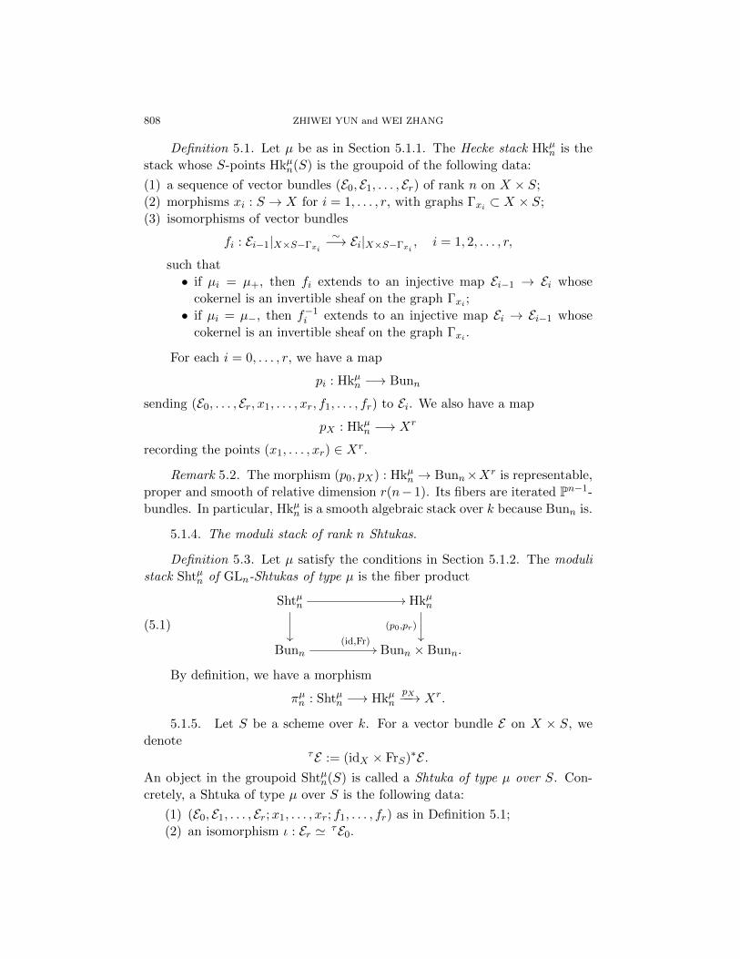
808 ZHIWEI YUN and WEI ZHANG
Definition 5.1. Let µ be as in Section 5.1.1. The Hecke stack Hkµn is the
stack whose S-points Hkµn(S) is the groupoid of the following data:
(1) a sequence of vector bundles (E0, E1, . . . , Er) of rank n on X × S;
(2) morphisms xi : S → X for i = 1, . . . , r, with graphs Γxi ⊂ X × S;
(3) isomorphisms of vector bundles
fi : Ei−1|X×S−Γxi
∼−→ Ei|X×S−Γxi, i = 1, 2, . . . , r,
such that
• if µi = µ+, then fi extends to an injective map Ei−1 → Ei whose
cokernel is an invertible sheaf on the graph Γxi ;
• if µi = µ−, then f−1i extends to an injective map Ei → Ei−1 whose
cokernel is an invertible sheaf on the graph Γxi .
For each i = 0, . . . , r, we have a map
pi : Hkµn −→ Bunn
sending (E0, . . . , Er, x1, . . . , xr, f1, . . . , fr) to Ei. We also have a map
pX : Hkµn −→ Xr
recording the points (x1, . . . , xr) ∈ Xr.
Remark 5.2. The morphism (p0, pX) : Hkµn → Bunn×Xr is representable,
proper and smooth of relative dimension r(n− 1). Its fibers are iterated Pn−1-
bundles. In particular, Hkµn is a smooth algebraic stack over k because Bunn is.
5.1.4. The moduli stack of rank n Shtukas.
Definition 5.3. Let µ satisfy the conditions in Section 5.1.2. The moduli
stack Shtµn of GLn-Shtukas of type µ is the fiber product
Shtµn //
Hkµn
(p0,pr)
Bunn(id,Fr)
// Bunn × Bunn.
(5.1)
By definition, we have a morphism
πµn : Shtµn −→ HkµnpX−−→ Xr.
5.1.5. Let S be a scheme over k. For a vector bundle E on X × S, we
denoteτE := (idX × FrS)∗E .
An object in the groupoid Shtµn(S) is called a Shtuka of type µ over S. Con-
cretely, a Shtuka of type µ over S is the following data:
(1) (E0, E1, . . . , Er;x1, . . . , xr; f1, . . . , fr) as in Definition 5.1;
(2) an isomorphism ι : Er ' τE0.

TAYLOR EXPANSION 809
The basic geometric properties of Shtµn are summarized in the following
theorem.
Theorem 5.4 (Drinfeld [5] for r = 2 ; Varshavsky [24, Prop 2.16, Th. 2.20]
in general).
(1) The stack Shtµn is a Deligne–Mumford stack locally of finite type.
(2) The morphism πµn : Shtµn → Xr is separated and smooth of relative dimen-
sion r(n− 1).
We briefly comment on the proof of the separatedness of πµn. Pick a place
x ∈ |X|, and consider the restriction of πµn to (X−x)r. By [24, Prop 2.16(a)],
Shtµn|(X−x)r is an increasing union of open substacks X1 ⊂ X2 ⊂ · · · where
each Xi ∼= [Vi/Gi] is the quotient of a quasi-projective scheme Vi over k by
a finite discrete group Gi. These Vi are obtained as moduli of Shtukas with
level structures at x and then truncated using stability conditions. Therefore,
each map Xi → (X − x)r is separated, hence so is πµn|(X−x)r . Since Xr is
covered by open subschemes of the form (X −x)r, the map πµn is separated.
5.1.6. The Picard stack PicX of line bundles on X acts on Bunn and on
Hkµn by tensoring on the vector bundles.
Similarly, the groupoid PicX(k) of line bundles over X acts on Shtµn. For
a line bundle L over X and (Ei;xi; fi; ι) ∈ Shtµn(S), we define L · (Ei;xi; fi; ι)to be (Ei ⊗OX L;xi; fi ⊗ idL; ι′), where ι′ is the isomorphism
Er⊗OXLι⊗idL−−−→ ((idX×FrS)∗E0)⊗OXL∼=(idX×FrS)∗(E0⊗OXL)= τ (E0 ⊗OX L).
5.2. Moduli of Shtukas for G = PGL2. Now we move on to G-Shtukas
where G = PGL2. Let BunG be the moduli stack of G-torsors over X.
5.2.1. Quotient by a Picard stack. Here and later we will consider quo-
tients of the form [Y/Q], where Y is an algebraic stack and Q is a Picard
stack such as PicX or PicX(k). Making such a quotient involves considering
2-categories a priori. However, according to [19, Lemme 4.7], whenever the
automorphism group of the identity object in Q injects to the automorphism
groups of objects in Y, the quotient [Y/Q] makes sense as a stack. This injec-
tivity condition will be satisfied in all situations we encounter in this paper.
We have BunG ∼= Bun2/PicX , where PicX acts on Bun2 by tensoring.
For each µ as in Section 5.1.1, we define
HkµG := Hkµ2/PicX .
For µ satisfying Section 5.1.2, we define
ShtµG := Shtµ2/PicX(k).

810 ZHIWEI YUN and WEI ZHANG
The actions of PicX and PicX(k) are those introduced in Section 5.1.6. The
maps pi : Hkµ2 → Bun2 are PicX -equivariant, and they induce maps
(5.2) pi : HkµG −→ BunG, 0 ≤ i ≤ r.
Lemma 5.5. For different choices µ and µ′ as in Section 5.1.1, there
are canonical isomorphisms Hkµ2∼= Hkµ
′
2 and HkµG∼= Hkµ
′
G . Moreover, these
isomorphisms respect the maps pi in (5.2).
Proof. For µr+ := (µ+, . . . , µ+), we denote the corresponding Hecke stack
by Hkr2. The S-points of Hkr2 classify a sequence of rank two vector bundles
on X × S together with embeddings
E0f1−→ E1
f2−→ · · · fr−→ Er
such that the cokernel of fi is an invertible sheaf supported on the graph of a
morphism xi : S → X.
We construct a morphism
φµ : Hkµ2 −→ Hkr2.
Consider a point (Ei;xi; fi) ∈ Hkµ2 (S). For i = 1, . . . , r, we define a divisor on
X × SDi :=
∑1≤j≤i,µj=µ−
Γxj .
Then we define
E ′i = Ei(Di).
If µi = µ+, then Di−1 = Di, and the map fi induces an embedding f ′i : E ′i−1 =
Ei−1(Di−1)→ Ei(Di−1) = E ′i. If µi = µ−, then Di = Di−1 + Γxi , and the map
fi : Ei → Ei−1 induces an embedding Ei−1 → Ei(Γxi), and hence an embedding
f ′i : E ′i−1 = Ei−1(Di−1)→ Ei(Di−1 + Γxi) = E ′i. The map φµ sends (Ei;xi; fi) to
(E ′i;xi; f ′i).We also have a morphism
ψµ : Hkr2−→Hkµ2
(E ′i;xi; f ′i) 7−→ (E ′i(−Di);xi; fi).
It is easy to check that φµ and ψµ are inverse to each other. This way we get a
canonical isomorphism Hkµ2∼= Hkr2, which is clearly PicX -equivariant. There-
fore, all HkµG are also canonically isomorphic to each other. In the construction
of φµ, the vector bundles Ei only change by tensoring with line bundles, there-
fore, the image of Ei in BunG remain unchanged. This shows that the canonical
isomorphisms between the HkµG respect the maps pi in (5.2).

TAYLOR EXPANSION 811
Lemma 5.6. There is a canonical Cartesian diagram
ShtµG
// HkµG
(p0,pr)
BunG(id,Fr)
// BunG × BunG.
(5.3)
In particular, for different choices of µ satisfying the conditions in Sec-
tion 5.1.2, the stacks ShtµG are canonically isomorphic to each other.
Proof. This follows from the Cartesian diagram (5.1) divided termwisely
by the Cartesian diagram
PicX(k) //
PicX
∆
PicX(id,Fr)
// PicX ×PicX .
By the above lemmas, we may unambiguously use the notation
(5.4) ShtrG; HkrG
for ShtµG and HkµG with any choice of µ. If r is fixed from the context, we
may also drop r from the notation and simply write ShtG. The morphism πµ2 :
Shtµ2 → Xr is invariant under the action of PicX(k) and induces a morphism
πG : ShtrG −→ Xr.
Theorem 5.4 has the following immediate consequence.
Corollary 5.7.
(1) The stack ShtrG is a Deligne–Mumford stack locally of finite type.
(2) The morphism πG : ShtrG → Xr is separated and smooth of relative dimen-
sion r.
5.3. Hecke correspondences. We define the rational Chow group of proper
cycles Chc,i(ShtrG)Q as in Section A.1. As in Section A.1.6, we also have a
Q-algebra cCh2r(ShtrG × ShtrG)Q that acts on Chc,i(ShtrG)Q. The goal of this
subsection is to define a ring homomorphism from the unramified Hecke algebra
H = Cc(K\G(A)/K,Q) to cCh2r(ShtrG × ShtrG)Q.
5.3.1. The stack ShtrG(hD). Recall from Section 3.1 that we have a basis
hD of H indexed by effective divisors D on X. For each effective divisor D =
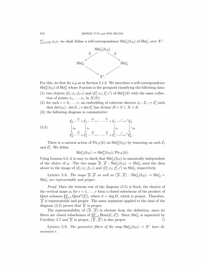
812 ZHIWEI YUN and WEI ZHANG∑x∈|X| nxx, we shall define a self-correspondence ShtrG(hD) of ShtrG over Xr:
ShtrG(hD)←−p
yy
−→p
%%
ShtrG
%%
ShtrG
yy
Xr.
For this, we first fix a µ as in Section 5.1.2. We introduce a self-correspondence
Shtµ2 (hD) of Shtµ2 whose S-points is the groupoid classifying the following data:
(1) two objects (Ei;xi; fi; ι) and (E ′i;xi; f ′i ; ι′) of Shtµ2 (S) with the same collec-
tion of points x1, . . . , xr in X(S);
(2) for each i = 0, . . . , r, an embedding of coherent sheaves φi : Ei → E ′i such
that det(φi) : det Ei → det E ′i has divisor D × S ⊂ X × S;
(3) the following diagram is commutative:
E0f1//
φ0
E1f2//
φ1
· · ·fr// Er
φr
ι// τE0
τφ0
E ′0f ′1// E ′1
f ′2// · · ·
f ′r// E ′r
ι′// τE ′0.
(5.5)
There is a natural action of PicX(k) on Shtµ2 (hD) by tensoring on each Eiand E ′i. We define
ShtrG(hD) := Shtµ2 (hD)/PicX(k).
Using Lemma 5.5, it is easy to check that ShtrG(hD) is canonically independent
of the choice of µ. The two maps ←−p ,−→p : ShtrG(hD) → ShtrG send the data
above to the image of (Ei;xi; fi; ι) and (E ′i;xi; f ′i ; ι′) in ShtrG respectively.
Lemma 5.8. The maps ←−p ,−→p as well as (←−p ,−→p ) : ShtrG(hD) → ShtrG ×ShtrG are representable and proper.
Proof. Once the bottom row of the diagram (5.5) is fixed, the choices of
the vertical maps φi for i = 1, . . . , r form a closed subscheme of the product of
Quot schemes∏ri=1 Quotd(E ′i), where d = degD, which is proper. Therefore,
−→p is representable and proper. The same argument applied to the dual of the
diagram (5.5) proves that ←−p is proper.
The representability of (←−p ,−→p ) is obvious from the definition, since its
fibers are closed subschemes of∏ri=1 Hom(Ei, E ′i). Since ShtrG is separated by
Corollary 5.7 and ←−p is proper, (←−p ,−→p ) is also proper.
Lemma 5.9. The geometric fibers of the map ShtrG(hD) → Xr have di-
mension r.

TAYLOR EXPANSION 813
The proof of this lemma will be postponed to Section 6.4.4, because the
argument will involve some auxiliary moduli spaces that we will introduce in
Section 6.3.
Granting Lemma 5.9, we have dim ShtrG(hD) = 2r. By Lemma 5.8, it
makes sense to push forward the fundamental cycle of ShtrG(hD) along the
proper map (←−p ,−→p ). Therefore, (←−p ,−→p )∗[ShtrG(hD)] defines an element in
cCh2r(ShtrG × ShtrG)Q (because ←−p is also proper). We define the Q-linear map
H : H −→ cCh2r(ShtrG × ShtrG)Q,(5.6)
hD 7−→ (←−p ×−→p )∗[ShtrG(hD)] for all effective divisors D.(5.7)
Proposition 5.10. The linear map H in (5.6) is a ring homomorphism.
Proof. Since hD form a Q-basis of H , it suffices to show that
(5.8) H(hDhD′) = H(hD) ∗H(hD′) ∈ cCh2r(ShtrG × ShtrG)Q
for any two effective divisors D and D′.
Let U = X − |D| − |D′|. Since hDhD′ is a linear combination of hE for
effective divisors E ≤ D+D′ such thatD+D′−E has even coefficients, the cycle
H(hDhD′) is supported on ∪E≤D+D′,D+D′−E evenShtrG(hE) = ShtrG(hD+D′).
The cycle H(hD) ∗H(hD′) is supported on the image of the projection
pr13 : ShtrG(hD)×−→p ,ShtrG,←−p ShtrG(hD′) −→ ShtrG × ShtrG,
which is easily seen to be contained in ShtrG(hD+D′). We see that both sides
of (5.8) are supported on Z := ShtrG(hD+D′).
By Lemma 5.9 applied to Z = ShtrG(hD+D′), the dimension of Z − Z|Uris strictly less than 2r. Therefore, the restriction map induces an isomorphism
(5.9) Ch2r(Z)Q∼−→ Ch2r(Z|Ur)Q.
Restricting the definition of H to U r, we get a linear map HU : H →cCh2r(ShtrG|Ur×ShtrG|Ur)Q. For any effective divisor E supported on |D|∪|D′|,the two projections ←−p ,−→p : ShtrG(hE)|Ur → ShtrG|Ur are finite etale. The
equality
(5.10) HU (hDhD′) = HU (hD) ∗HU (hD′) ∈ Ch2r(Z|Ur)Qis well known. By (5.9), this implies the equality (5.8) where both sides are
interpreted as elements in Ch2r(Z)Q, and a fortiori as elements in cCh2r(ShtrG×ShtrG)Q.
Remark 5.11. Let g = (gx) ∈ G(A), and let f = 1KgK ∈ H be the
characteristic function of the double coset KgK in G(A). Traditionally, one
defines a self-correspondence Γ(g) of ShtrG|(X−S)r over (X − S)r, where S is
the finite set of places where gx /∈ Kx (see [15, Construction 2.20]). The two
projections ←−p ,−→p : Γ(g) → ShtrG|(X−S)r are finite etale. The disadvantage of

814 ZHIWEI YUN and WEI ZHANG
this definition is that we need to remove the bad points S that depend on f , so
one is forced to work only with the generic fiber of ShtrG over Xr if one wants
to consider the actions of all Hecke functions. Our definition of H(f) for any
f ∈H gives a correspondence for the whole ShtrG. It is easy to check that for
f = 1KgK , our cycle H(f)|(X−S)r , which is a linear combination of the cycles
ShtrG(hD)|(X−S)r for divisors D supported on S, is the same cycle as Γ(g).
Thus, our definition of the Hecke algebra action extends the traditional one.
5.3.2. A variant. Later we will consider the stack Sht′rG := ShtrG ×Xr X ′r
defined using the double cover X ′ → X. Let Sht′rG(hD) = ShtrG(hD) ×Xr X ′r.
Then we have natural maps
←−p ′,−→p ′ : Sht′rG(hD) −→ Sht′rG.
The analogs of Lemmas 5.8 and 5.9 for Sht′rG(hD) follow from the original
statements. The map hD 7→ (←−p ′ × −→p ′)∗[Sht′rG(hD)] ∈ cCh2r(Sht′rG × Sht′rG)Qthen gives a ring homomorphism H ′:
H ′ : H −→ cCh2r(Sht′rG × Sht′rG)Q.
5.3.3. Notation. By Section A.1.6, the Q-algebra cCh2r(Sht′rG × Sht′rG)Qacts on Chc,∗(Sht′rG)Q. Hence the Hecke algebra H also acts on Chc,∗(Sht′rG)Qvia the homomorphism H ′. For f ∈H , we denote its action on Chc,∗(Sht′rG)Qby
f ∗ (−) : Chc,∗(Sht′rG)Q −→ Chc,∗(Sht′rG)Q.
Recall that the Chow group Chc,∗(ShtrG)Q (or Chc,∗(Sht′rG)Q) is equipped
with an intersection pairing between complementary degrees; see Section A.1.4.
Lemma 5.12. The action of any f ∈H on Chc,∗(ShtrG)Q or Chc,∗(Sht′rG)Qis self-adjoint with respect to the intersection pairing.
Proof. It suffices to prove self-adjointness for hD for all effective divisorsD.
We give the argument for ShtrG, and the case of Sht′rG can be proved in the
same way. For ζ1 ∈ Chc,i(ShtrG)Q and ζ2 ∈ Chc,2r−i(ShtrG)Q, the intersection
number 〈hD ∗ ζ1, ζ2〉ShtrGis the same as the following intersection number in
ShtrG × ShtrG:
〈ζ1 × ζ2, (←−p ,−→p )∗[ShtrG(hD)]〉ShtrG×ShtrG
.
We will construct an involution τ on ShtrG(hD) such that the following diagram
is commutative:
ShtrG(hD)
(←−p ,−→p )
τ// ShtrG(hD)
(←−p ,−→p )
ShtrG × ShtrGσ12
// ShtrG × ShtrG.
(5.11)

TAYLOR EXPANSION 815
Here σ12 in the bottom row means flipping two factors. Once we have such a
diagram, we can apply τ to ShtrG(hD) and σ12 to ShtrG × ShtrG and get
〈ζ1 × ζ2, (←−p ,−→p )∗[ShtrG(hD)]〉ShtrG×ShtrG
= 〈ζ2 × ζ1, (←−p ,−→p )∗[ShtrG(hD)]〉ShtrG×ShtrG
,
which is the same as the self-adjointness for h ∗ (−):
〈hD ∗ ζ1, ζ2〉ShtrG= 〈hD ∗ ζ2, ζ1〉ShtrG
= 〈ζ1, hD ∗ ζ2〉ShtrG.
We pick any µ as in Section 5.1.2, and we identify ShtrG with ShtµG =
Shtµ2/PicX(k). We use −µ to denote the negated tuple if we think of µ ∈ ±1rusing the sgn map. We consider the composition
δ : ShtµGδ′−→ Sht−µG
∼= ShtµG,
where δ′(Ei;xi; fi; ι) = (E∨i ;xi; (f∨i )−1; (ι∨)−1), and the second map is the
canonical isomorphism Sht−µG∼= ShtµG given by Lemma 5.6.
Similarly, we define τ as the composition
(5.12) τ : ShtµG(hD)τ ′−→ Sht−µG (hD) ∼= ShtµG(hD),
where τ ′ sends the diagram (5.5) to the diagram
E ′∨0f ′∨−11//
φ∨0
E ′∨1f ′∨−12//
φ∨1
· · ·f ′∨−1r// E ′∨r
φ∨r
ι′∨−1// τE ′∨0
τφ∨0
E∨0f∨−11// E∨1
f∨−12// · · ·
f∨−1r// E∨r
ι∨−1// τE∨0
(5.13)
and the second map in (5.12) is the canonical isomorphism Sht−µG (hD) ∼=ShtµG(hD) given by the analog of Lemma 5.6. It is clear from the definition
that if we replace the bottom arrow of (5.11) with σ12 (δ × δ) (i.e., the map
(a, b) 7→ (δ(b), δ(a))), then the diagram is commutative.
We claim that δ is the identity map for ShtµG. In fact, δ turns (Ei;xi; fi; ι) ∈ShtµG into (E∨i (Di);xi; (f∨i )−1; (ι∨)−1), where Di =
∑1≤j≤i sgn(µj)Γxj . Note
that we have a canonical isomorphism E∨i ∼= Ei ⊗ (det Ei)−1 and isomorphisms
det Ei ∼= (det E0)(Di) induced by the fi. Therefore, we get a canonical isomor-
phism E∨i (Di) ∼= Ei ⊗ (det Ei)−1 ⊗ O(Di) ∼= Ei ⊗ (det E0)−1 compatibly with
the maps (f∨i )−1 and fi, and also compatible with (ι∨)−1 and ι. Therefore,
δ(Ei;xi; fi; ι) is canonically isomorphic to (Ei;xi; fi; ι) up to tensoring with
det(E0). This shows that δ is the identity map of ShtµG.
Since δ = id, the diagram (5.11) is also commutative. This finishes the
proof.

816 ZHIWEI YUN and WEI ZHANG
5.4. Moduli of Shtukas for the torus T .
5.4.1. Recall that ν : X ′ → X is an etale double covering with X ′ also
geometrically connected. Let σ ∈ Gal(X ′/X) be the nontrivial involution.
Let ‹T be the two-dimensional torus over X defined as‹T := ResX′/X Gm.
We have a natural homomorphism Gm → ‹T . We define a one-dimensional
torus over X:
T := ‹T/Gm = (ResX′/X Gm)/Gm.
Let BunT be the moduli stack of T -torsors over X. Then we have a
canonical isomorphism of stacks
BunT ∼= PicX′ /PicX .
In particular, BunT is a Deligne–Mumford stack whose coarse moduli space is
a group scheme with two components, and its neutral component is an abelian
variety over k.
5.4.2. Specializing Definition 5.1 to the case n = 1 and replacing the
curve X with its double cover X ′, we get the Hecke stack Hkµ1,X′ . This makes
sense for any tuple µ as in Section 5.1.1.
Now assume that µ satisfies the conditions in Section 5.1.2. We may view
each µi as a coweight for GL1 = Gm in an obvious way: µ+ means 1 and
µ− means −1. Specializing Definition 5.3 to the case n = 1 and replacing X
with X ′, we get the moduli stack Shtµ1,X′ of rank one Shtukas over X ′ of type µ.
We define
ShtµT
:= Shtµ1,X′ .
We have a Cartesian diagram
ShtµT
// Hkµ1,X′
(p0,pr)
PicX′(id,Fr)
// PicX′ ×PicX′ .
We also have a morphism
πµT
: ShtµT−→ Hkµ1,X′
pX′−−→ X ′r.
5.4.3. Fix µ as in Section 5.1.2. Concretely, for any k-scheme S, ShtµT
(S)
classifies the following data:
(1) a line bundle L over X ′ × S;
(2) morphisms x′i : S → X ′ for i = 1, . . . , r, with graphs Γx′i ⊂ X′ × S;
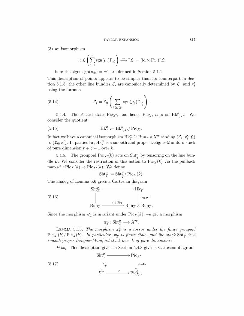
TAYLOR EXPANSION 817
(3) an isomorphism
ι : L(
r∑i=1
sgn(µi)Γx′i
)∼−→ τL := (id× FrS)∗L;
here the signs sgn(µ±) = ±1 are defined in Section 5.1.1.
This description of points appears to be simpler than its counterpart in Sec-
tion 5.1.5: the other line bundles Li are canonically determined by L0 and x′iusing the formula
(5.14) Li = L0
Ñ ∑1≤j≤i
sgn(µj)Γx′j
é.
5.4.4. The Picard stack PicX′ , and hence PicX , acts on Hkµ1,X′ . We
consider the quotient
(5.15) HkµT := Hkµ1,X′/PicX .
In fact we have a canonical isomorphism HkµT∼= BunT ×X ′r sending (Li;x′i; fi)
to (L0;x′i). In particular, HkµT is a smooth and proper Deligne–Mumford stack
of pure dimension r + g − 1 over k.
5.4.5. The groupoid PicX′(k) acts on ShtµT
by tensoring on the line bun-
dle L. We consider the restriction of this action to PicX(k) via the pullback
map ν∗ : PicX(k)→ PicX′(k). We define
ShtµT := ShtµT/PicX(k).
The analog of Lemma 5.6 gives a Cartesian diagram
ShtµT
// HkµT
(p0,pr)
BunT(id,Fr)
// BunT × BunT .
(5.16)
Since the morphism πµT
is invariant under PicX(k), we get a morphism
πµT : ShtµT −→ X ′r.
Lemma 5.13. The morphism πµT is a torsor under the finite groupoid
PicX′(k)/PicX(k). In particular, πµT is finite etale, and the stack ShtµT is a
smooth proper Deligne–Mumford stack over k of pure dimension r.
Proof. This description given in Section 5.4.3 gives a Cartesian diagram
ShtµT
πµT
// PicX′
id−Fr
X ′rφ
// Pic0X′ ,
(5.17)

818 ZHIWEI YUN and WEI ZHANG
where φ(x′1, . . . , x′r) = OX′(
∑ri=1 sgn(µi)x
′i). Dividing the top row of the dia-
gram (5.17) by PicX(k) we get a Cartesian diagram
ShtµT
πµT
// PicX′ /(PicX(k))
id−Fr
X ′rφ
// Pic0X′ .
Since the right vertical map id − Fr : PicX′ /(PicX(k)) → Pic0X′ is a torsor
under PicX′(k)/PicX(k), so is πµT .
5.4.6. Changing µ. For a different choice µ′ as in 5.1.1, we have a canonical
isomorphism
(5.18) HkµT
∼−→ Hkµ′
T
sending (Li;x′i; fi) to (Ki; y′i; gi) where
(5.19) y′i =
x′i if µi = µ′i,
σ(x′i) if µi 6= µ′i,
and
(5.20) Ki = L0
Ñ ∑1≤j≤i
sgn(µ′j)Γy′j
é.
The rational maps gi : Ki−1 99K Ki is the one corresponding to the identity
map on L0 via the description (5.20). Note that we have
Ki = Li ⊗OX×S OX×S
Ñ ∑1≤j≤i
sgn(µ′j)− sgn(µj)
2Γxj
é,
where xi : S → X is the image of x′i. Therefore, Ki has the same image as Liin BunT . The isomorphism (5.18) induces an isomorphism
(5.21) HkµT∼−→ Hkµ
′
T .
From the construction and the above discussion, this isomorphism preserves
the maps pi to BunT but does not preserve the projections to X ′r. (It only
preserves the further projection to Xr.)
Since the isomorphism (5.21) preserves the maps p0 and pr, the diagram
(5.16) implies a canonical isomorphism
(5.22) ιµ,µ′ : ShtµT∼−→ Shtµ
′
T .
Just as the map (5.21), ιµ,µ′ does not respect the maps πµT and πµ′
T from ShtµTand Shtµ
′
T to X ′r: it only respects their further projections to Xr.

TAYLOR EXPANSION 819
5.5. The Heegner–Drinfeld cycles.
5.5.1. We have a morphism
Π : BunT −→BunG
(L mod PicX) 7−→ (ν∗L mod PicX).
5.5.2. For any µ as in Section 5.1.2, we define a morphism
θµ : ShtµT−→ Shtµ2
as follows. Let (L;x′i; ι) ∈ ShtµT
(S) as in the description in Section 5.4.3. Let
L0 = L. We may define the line bundles Li using (5.14). Then there are
natural maps gi : Li−1 → Li if µi = µ+ or gi : Li → Li−1 if µi = µ−. Let
νS = ν × idS : X ′ × S → X × S be the base change of ν. We define
Ei = νS∗Li,
with the maps fi : Ei−1 → Ei or Ei → Ei−1 induced from gi. The isomorphism ι
then induces an isomorphism
: Er = νS∗LrνS∗ι−−→ νS∗(idX′ × FrS)∗L0
∼= (idX × FrS)∗νS∗L0 = τE0.
Let xi = ν x′i. The morphism θµ then sends (L;x′i; ι) to (Ei;xi; fi; ). Clearly
θµ is equivariant with respect to the PicX(k)-actions. Passing to the quotients,
we get a morphism
θµ
: ShtµT −→ ShtµG.
For a different µ′, the canonical isomorphism ιµ,µ′ in (5.22) intertwines the
maps θµ
and θµ′
; i.e., we have a commutative diagram
ShtµT
ιµ,µ′
θµ
// ShtµG
Shtµ′
Tθµ′
// Shtµ′
G ,
where the right vertical map is the canonical isomorphism in Lemma 5.6. By
our identification of ShtµG for different µ (cf. (5.4)), we get a morphism, still
denoted by θµ,
θµ
: ShtµT −→ ShtrG.
5.5.3. By construction we have a commutative diagram
ShtµT
πµT
θµ
// ShtrG
πG
X ′rνr
// Xr.

820 ZHIWEI YUN and WEI ZHANG
Recall that
Sht′rG := ShtrG ×Xr X ′r.
Then the map θµ
factors through a morphism
θµ : ShtµT −→ Sht′rG
over X ′r. Since ShtµT is proper of dimension r, θµ∗ [ShtµT ] is a proper cycle class
in Sht′rG of dimension r.
Definition 5.14. The Heegner–Drinfeld cycle of type µ is the direct image
of [ShtµT ] under θµ:
θµ∗ [ShtµT ] ∈ Chc,r(Sht′rG)Q.
Recall from Proposition 5.10 and Section 5.3.3 that we have an action of
H on Chc,r(Sht′rG)Q. Since
dim ShtµT = r =1
2dim Sht′rG,
both θµ∗ [ShtµT ] and f ∗ θµ∗ [ShtµT ] for any function f ∈ H are proper cycle
classes in ShtrG of complementary dimension, and they define elements in
Chc,r(Sht′rG)Q. The following definition then makes sense.
Definition 5.15. Let f ∈ H be an unramified Hecke function. We define
the following intersection number:
Ir(f) := 〈θµ∗ [ShtµT ], f ∗ θµ∗ [ShtµT ]〉Sht′rG∈ Q.
5.5.4. Changing µ. For different µ and µ′ as in Section 5.1.2, the Heegner–
Drinfeld cycles θµ∗ [ShtµT ] and θµ′∗ [Shtµ
′
T ] are different. Therefore, a priori the
intersection number Ir(f) depends on µ. However, we have
Lemma 5.16. The intersection number Ir(f) for any f ∈ H is indepen-
dent of the choice of µ.
Proof. Let Zµ denote the cycle θµ∗ [ShtµT ]. Using the isomorphism ιµ,µ′
in (5.22), we see that Zµ and Zµ′
are transformed to each other under the
involution σ(µ, µ′) : Sht′rG = ShtrG ×Xr X ′r → ShtrG ×Xr X ′r = Sht′rG, which
is the identity on ShtrG and on X ′r sends (x′1, . . . , x′r) to (y′1, . . . , y
′r) using the
formula (5.19). Since σ(µ, µ′) is the identity on ShtrG, it commutes with the
Hecke action on Chc,r(Sht′rG)Q. Therefore, we have
〈Zµ, f ∗ Zµ〉Sht′rG= 〈σ(µ, µ′)∗Z
µ, σ(µ, µ′)∗(f ∗ Zµ)〉Sht′rG
= 〈σ(µ, µ′)∗Zµ, f ∗ (σ(µ, µ′)∗Z
µ)〉Sht′rG= 〈Zµ′ , f ∗ Zµ′〉Sht′rG
.
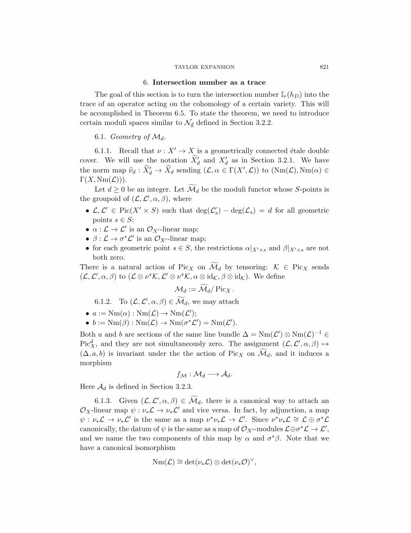
TAYLOR EXPANSION 821
6. Intersection number as a trace
The goal of this section is to turn the intersection number Ir(hD) into the
trace of an operator acting on the cohomology of a certain variety. This will
be accomplished in Theorem 6.5. To state the theorem, we need to introduce
certain moduli spaces similar to Nd defined in Section 3.2.2.
6.1. Geometry of Md.
6.1.1. Recall that ν : X ′ → X is a geometrically connected etale double
cover. We will use the notation “X ′d and X ′d as in Section 3.2.1. We have
the norm map νd : “X ′d → “Xd sending (L, α ∈ Γ(X ′,L)) to (Nm(L),Nm(α) ∈Γ(X,Nm(L))).
Let d ≥ 0 be an integer. Let ›Md be the moduli functor whose S-points is
the groupoid of (L,L′, α, β), where
• L,L′ ∈ Pic(X ′ × S) such that deg(L′s) − deg(Ls) = d for all geometric
points s ∈ S;
• α : L → L′ is an OX′-linear map;
• β : L → σ∗L′ is an OX′-linear map;
• for each geometric point s ∈ S, the restrictions α|X′×s and β|X′×s are not
both zero.
There is a natural action of PicX on ›Md by tensoring: K ∈ PicX sends
(L,L′, α, β) to (L ⊗ ν∗K,L′ ⊗ ν∗K, α⊗ idK, β ⊗ idK). We define
Md := ›Md/PicX .
6.1.2. To (L,L′, α, β) ∈ ›Md, we may attach
• a := Nm(α) : Nm(L)→ Nm(L′);• b := Nm(β) : Nm(L)→ Nm(σ∗L′) = Nm(L′).
Both a and b are sections of the same line bundle ∆ = Nm(L′)⊗ Nm(L)−1 ∈PicdX , and they are not simultaneously zero. The assignment (L,L′, α, β) 7→(∆, a, b) is invariant under the the action of PicX on ›Md, and it induces a
morphism
fM :Md −→ Ad.
Here Ad is defined in Section 3.2.3.
6.1.3. Given (L,L′, α, β) ∈ ›Md, there is a canonical way to attach an
OX -linear map ψ : ν∗L → ν∗L′ and vice versa. In fact, by adjunction, a map
ψ : ν∗L → ν∗L′ is the same as a map ν∗ν∗L → L′. Since ν∗ν∗L ∼= L ⊕ σ∗Lcanonically, the datum of ψ is the same as a map of OX′-modules L⊕σ∗L → L′,and we name the two components of this map by α and σ∗β. Note that we
have a canonical isomorphism
Nm(L) ∼= det(ν∗L)⊗ det(ν∗O)∨,

822 ZHIWEI YUN and WEI ZHANG
and likewise for L′. Therefore, det(ψ) : det(ν∗L)→ det(ν∗L′) can be identified
with a map Nm(L)→ Nm(L′), which is given by
(6.1) det(ψ) = Nm(α)−Nm(β) = a− b : Nm(L) −→ Nm(L′).
The composition δ fM : Md → Ad → “Xd takes (L,L′, α, β) to the pair
(∆ = Nm(L′)⊗Nm(L)−1, det(ψ)).
6.1.4. We give another description of Md. We have a map ια :Md→ “X ′dsending (L,L′, α, β) to the line bundle L′ ⊗ L−1 and its section given by α.
Similarly, we have a map ιβ : Md → “X ′d sending (L,L′, α, β) to the line
bundle σ∗L′ ⊗ L−1 and its section given by β. Note that the line bundles
underlying ια(L,L′, α, β) and ιβ(L,L′, α, β) have the same norm ∆ = Nm(L′)⊗Nm(L)−1 ∈ PicdX . Since α and β are not both zero, we get a map
ι = (ια, ιβ) :Md −→ “X ′d ×PicdX“X ′d − Z ′d,
where the fiber product on the right-hand side is taken with respect to the
map “X ′d → PicdX′Nm−−→ PicdX , and Z ′d := PicdX′ ×PicdX
PicdX′ is embedded into“X ′d ×PicdX“X ′d by viewing PicdX′ as the zero section of “X ′d in both factors.
Proposition 6.1.
(1) The morphism ι is an isomorphism of functors, and Md is a proper
Deligne–Mumford stack over k.3
(2) For d ≥ 2g′ − 1, Md is a smooth Deligne–Mumford stack over k of pure
dimension 2d− g + 1.
(3) The morphism νd : “X ′d → “Xd is proper.
(4) We have a Cartesian diagram
Md ι
//
fM
“X ′d ×PicdX“X ′d
νd×νd
Ad
// “Xd ×PicdX“Xd.
(6.2)
Moreover, the map fM is proper.
Proof. (1) Let (PicX′ ×PicX′)d be the disjoint union of PiciX′ ×Pici+dX′ over
all i ∈ Z. Consider the morphism
θ : (PicX′ ×PicX′)d/PicX −→ PicdX′ ×PicdXPicdX′
(the fiber product is taken with respect to the norm map) that sends (L,L′) to
(L′ ⊗ L−1, σ∗L′ ⊗ L−1, τ), where τ is the tautological isomorphism between
3The properness of Md will not be used elsewhere in this paper.
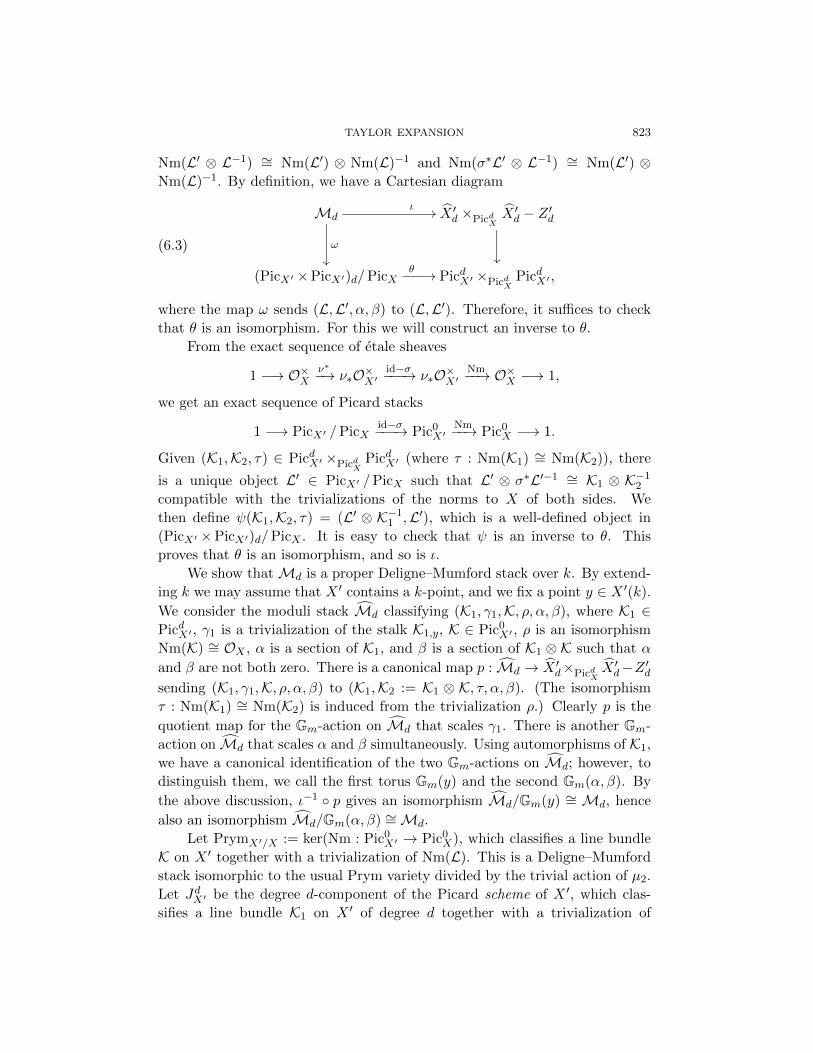
TAYLOR EXPANSION 823
Nm(L′ ⊗ L−1) ∼= Nm(L′) ⊗ Nm(L)−1 and Nm(σ∗L′ ⊗ L−1) ∼= Nm(L′) ⊗Nm(L)−1. By definition, we have a Cartesian diagram
Mdι//
ω
“X ′d ×PicdX“X ′d − Z ′d
(PicX′ ×PicX′)d/PicXθ// PicdX′ ×PicdX
PicdX′ ,
(6.3)
where the map ω sends (L,L′, α, β) to (L,L′). Therefore, it suffices to check
that θ is an isomorphism. For this we will construct an inverse to θ.
From the exact sequence of etale sheaves
1 −→ O×Xν∗−→ ν∗O×X′
id−σ−−−→ ν∗O×X′Nm−−→ O×X −→ 1,
we get an exact sequence of Picard stacks
1 −→ PicX′ /PicXid−σ−−−→ Pic0
X′Nm−−→ Pic0
X −→ 1.
Given (K1,K2, τ) ∈ PicdX′ ×PicdXPicdX′ (where τ : Nm(K1) ∼= Nm(K2)), there
is a unique object L′ ∈ PicX′ /PicX such that L′ ⊗ σ∗L′−1 ∼= K1 ⊗ K−12
compatible with the trivializations of the norms to X of both sides. We
then define ψ(K1,K2, τ) = (L′ ⊗ K−11 ,L′), which is a well-defined object in
(PicX′ ×PicX′)d/PicX . It is easy to check that ψ is an inverse to θ. This
proves that θ is an isomorphism, and so is ι.
We show thatMd is a proper Deligne–Mumford stack over k. By extend-
ing k we may assume that X ′ contains a k-point, and we fix a point y ∈ X ′(k).
We consider the moduli stack ”Md classifying (K1, γ1,K, ρ, α, β), where K1 ∈PicdX′ , γ1 is a trivialization of the stalk K1,y, K ∈ Pic0
X′ , ρ is an isomorphism
Nm(K) ∼= OX , α is a section of K1, and β is a section of K1 ⊗ K such that α
and β are not both zero. There is a canonical map p : ”Md → “X ′d×PicdX“X ′d−Z ′d
sending (K1, γ1,K, ρ, α, β) to (K1,K2 := K1 ⊗ K, τ, α, β). (The isomorphism
τ : Nm(K1) ∼= Nm(K2) is induced from the trivialization ρ.) Clearly p is the
quotient map for the Gm-action on ”Md that scales γ1. There is another Gm-
action on ”Md that scales α and β simultaneously. Using automorphisms of K1,
we have a canonical identification of the two Gm-actions on ”Md; however, to
distinguish them, we call the first torus Gm(y) and the second Gm(α, β). By
the above discussion, ι−1 p gives an isomorphism ”Md/Gm(y) ∼= Md, hence
also an isomorphism ”Md/Gm(α, β) ∼=Md.
Let PrymX′/X := ker(Nm : Pic0X′ → Pic0
X), which classifies a line bundle
K on X ′ together with a trivialization of Nm(L). This is a Deligne–Mumford
stack isomorphic to the usual Prym variety divided by the trivial action of µ2.
Let JdX′ be the degree d-component of the Picard scheme of X ′, which clas-
sifies a line bundle K1 on X ′ of degree d together with a trivialization of
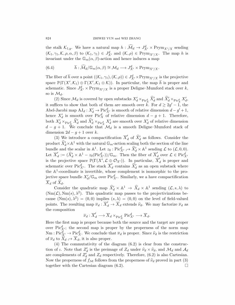
824 ZHIWEI YUN and WEI ZHANG
the stalk K1,y. We have a natural map h : ”Md → JdX′ × PrymX′/X sending
(K1, γ1,K, ρ, α, β) to (K1, γ1) ∈ JdX′ and (K, ρ) ∈ PrymX′/X . The map h is
invariant under the Gm(α, β)-action and hence induces a map
(6.4) h : ”Md/Gm(α, β) ∼=Md −→ JdX′ × PrymX′/X .
The fiber of h over a point ((K1, γ1), (K, ρ)) ∈ JdX′×PrymX′/X is the projective
space P(Γ(X ′,K1) ⊕ Γ(X ′,K1 ⊗ K)). In particular, the map h is proper and
schematic. Since JdX′ × PrymX′/X is a proper Deligne–Mumford stack over k,
so is Md.
(2) SinceMd is covered by open substacks X ′d×PicdX“X ′d and “X ′d×PicdX
X ′d,
it suffices to show that both of them are smooth over k. For d ≥ 2g′ − 1, the
Abel-Jacobi map AJd : X ′d → PicdX′ is smooth of relative dimension d− g′+ 1,
hence X ′d is smooth over PicdX of relative dimension d − g + 1. Therefore,
both X ′d ×PicdX“X ′d and “X ′d ×PicdX
X ′d are smooth over X ′d of relative dimension
d − g + 1. We conclude that Md is a smooth Deligne–Mumford stack of
dimension 2d− g + 1 over k.
(3) We introduce a compactification X′d of “X ′d as follows. Consider the
product “X ′d×A1 with the natural Gm-action scaling both the section of the line
bundle and the scalar in A1. Let z0 : PicdX′ → “X ′d × A1 sending L to (L, 0, 0).
Let X′d := (“X ′d × A1 − z0(PicdX′))/Gm. Then the fiber of X
′d over L ∈ PicdX′
is the projective space P(Γ(X ′,L ⊕ OX′)). In particular, X′d is proper and
schematic over PicdX′ . The stack X′d contains “X ′d as an open substack where
the A1-coordinate is invertible, whose complement is isomorphic to the pro-
jective space bundle X ′d/Gm over PicdX′ . Similarly, we a have compactification
Xd of “Xd.
Consider the quadratic map “X ′d × A1 → “Xd × A1 sending (L, s, λ) to
(Nm(L),Nm(s), λ2). This quadratic map passes to the projectivizations be-
cause (Nm(s), λ2) = (0, 0) implies (s, λ) = (0, 0) on the level of field-valued
points. The resulting map νd : X′d → Xd extends νd. We may factorize νd as
the composition
νd : X′d −→ Xd ×PicdX
PicdX′ −→ Xd.
Here the first map is proper because both the source and the target are proper
over PicdX′ ; the second map is proper by the properness of the norm map
Nm : PicdX′ → PicdX . We conclude that νd is proper. Since νd is the restriction
of νd to “Xd → Xd, it is also proper.
(4) The commutativity of the diagram (6.2) is clear from the construc-
tion of ι. Note that Z ′d is the preimage of Zd under νd × νd, and Md and Adare complements of Z ′d and Zd respectively. Therefore, (6.2) is also Cartesian.
Now the properness of fM follows from the properness of νd proved in part (3)
together with the Cartesian diagram (6.2).

TAYLOR EXPANSION 825
6.2. A formula for Ir(hD).
6.2.1. The correspondence HkµM,d. Fix any tuple µ = (µ1, . . . , µr) as in
Section 5.1.1. We define ›Hkµ
M,d to be the moduli functor whose S-points
classify the following data:
(1) for i = 1, . . . , r, a map x′i : S → X ′ with graph Γx′i ;
(2) for each i = 0, 1, . . . , r, an S-point (Li,L′i, αi, βi) of ›Md:
αi : Li −→ L′i, βi : Li −→ σ∗L′i;(3) a commutative diagram of OX′-linear maps between line bundles on X ′
L0
α0
f1// L1
α1
f2// · · ·
fr// Lr
αr
L′0f ′1// L′1
f ′2// · · ·
f ′r// L′r,
(6.5)
where the top and bottom rows are S-points of HkµT over the same point
(x′1, . . . , x′r) ∈ X ′r(S), such that the following diagram is also commutative:
L0
β0
f1// L1
β1
f2// · · ·
fr// Lr
βr
σ∗L′0σ∗f ′1
// σ∗L′1σ∗f ′2
// · · ·σ∗f ′r// σ∗L′r.
(6.6)
There is an action of PicX on ›Hkµ
M,d by tensoring on the line bundles Li and L′i.We define
HkµM,d := ›Hkµ
M,d/PicX .
The same argument as Section 5.4.6 (applying the isomorphism (5.21) to both
rows of (6.6)) shows that for different choices of µ, the stacks HkµM,d are canon-
ically isomorphic to each other. However, as in the case for HkµT , the morphism
HkµM,d → X ′r does depend on µ.
6.2.2. Let γi : HkµM,d →Md be the projections given by taking the dia-
gram (6.5) to its i-th column. It is clear that this map is schematic, therefore,
HkµM,d itself is a Deligne–Mumford stack.
In the diagram (6.5), the line bundles ∆i = Nm(L′i) ⊗ Nm(Li)−1 are
all canonically isomorphic to each other for i = 0, . . . , r. Also the sections
ai = Nm(αi) (resp. bi = Nm(βi)) of ∆i can be identified with each other for
all i under the isomorphisms between the ∆i’s. Therefore, composing γi with
the map fM : Md → Ad all give the same map. We may view HkµM,d as a
self-correspondence of Md over Ad via the maps (γ0, γr).
There is a stronger statement. Let us define ‹Ad ⊂ “X ′d ×PicdX“Xd to be
the preimage of Ad under Nm×id : “X ′d ×PicdX“Xd → “Xd ×PicdX
“Xd. Then ‹Ad

826 ZHIWEI YUN and WEI ZHANG
classifies triples (K, α, b), where K ∈ PicX′ , α is a section of K, and b is a
section of Nm(K) such that α and b are not simultaneously zero. Then fMfactors through the map
fM :Md −→ ‹Adsending (L,L′, α, β) to (L′ ⊗ L−1, α,Nm(β)).
Consider a point of HkµM,d giving, among others, the diagram (6.5). Since
the maps fi and f ′i are simple modifications at the same point x′i, the line
bundles L′i ⊗ L−1i are all isomorphic to each other for all i = 0, 1, . . . , r. Un-
der these isomorphisms, their sections given by αi correspond to each other.
Therefore, the maps fM γi : HkµM,d → ‹Ad are the same for all i.
6.2.3. The particular case r = 1 and µ = (µ+) gives a moduli space
H := Hk1M,d classifying commutative diagrams up to simultaneous tensoring
by PicX :
L0f//
α0
L1
α1
L0f
//
β0
L1
β1
L′0f ′// L′1, σ∗L′0
σ∗f ′// σ∗L′1.
(6.7)
such that the cokernel of f and f ′ are invertible sheaves supported at the same
point x′ ∈ X ′, and the data (L0,L′0, α0, β0) and (L1,L′1, α1, β1) are objects
of Md.
We have two maps (γ0, γ1) : H → Md, and we view H as a self-corre-
spondence of Md over Ad. We also have a map p : H → X ′ recording the
point x′ (support of L1/L0 and L′1/L′0).
The following lemma follows directly from the definition of HkµM,d.
Lemma 6.2. As a self-correspondence of Md, HkµM,d is canonically iso-
morphic to the r-fold composition of H:
HkµM,d∼= H×γ1,Md,γ0 ×H×γ1,Md,γ0 × · · · ×γ1,Md,γ0 H.
6.2.4. Let A♦d ⊂ Ad be the open subset consisting of (∆, a, b) where
b 6= 0; i.e., A♦d = “Xd×PicdXXd under the isomorphism (3.3). LetM♦d , HkµM♦,d
and H♦ be the preimages of A♦d in Md, HkµM,d and H.
Lemma 6.3. Let I ′d ⊂ X ′d × X ′ be the incidence scheme; i.e., I ′d → X ′dis the universal family of degree d effective divisors on X ′. There is a natural
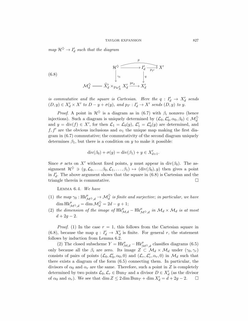
TAYLOR EXPANSION 827
map H♦ → I ′d such that the diagram
H♦p
))//
γ1
I ′d
q
pI′// X ′
M♦d “X ′d ×PicdXX ′d
pr2// X ′d
(6.8)
is commutative and the square is Cartesian. Here the q : I ′d → X ′d sends
(D, y) ∈ X ′d ×X ′ to D − y + σ(y), and pI′ : I ′d → X ′ sends (D, y) to y.
Proof. A point in H♦ is a diagram as in (6.7) with βi nonzero (hence
injections). Such a diagram is uniquely determined by (L0,L′0, α0, β0) ∈ M♦dand y = div(f) ∈ X ′, for then L1 = L0(y), L′1 = L′0(y) are determined, and
f, f ′ are the obvious inclusions and α1 the unique map making the first dia-
gram in (6.7) commutative; the commutativity of the second diagram uniquely
determines β1, but there is a condition on y to make it possible:
div(β0) + σ(y) = div(β1) + y ∈ X ′d+1.
Since σ acts on X ′ without fixed points, y must appear in div(β0). The as-
signment H♦ 3 (y,L0, . . . , β0,L1, . . . , β1) 7→ (div(β0), y) then gives a point
in I ′d. The above argument shows that the square in (6.8) is Cartesian and the
triangle therein is commutative.
Lemma 6.4. We have
(1) the map γ0 : HkµM♦,d →M♦d is finite and surjective; in particular, we have
dim HkµM♦,d = dimM♦d = 2d− g + 1;
(2) the dimension of the image of HkµM,d − HkµM♦,d in Md ×Md is at most
d+ 2g − 2.
Proof. (1) In the case r = 1, this follows from the Cartesian square in
(6.8), because the map q : I ′d → X ′d is finite. For general r, the statement
follows by induction from Lemma 6.2.
(2) The closed subscheme Y = HkµM,d − HkµM♦,d classifies diagrams (6.5)
only because all the βi are zero. Its image Z ⊂ Md × Md under (γ0, γr)
consists of pairs of points (L0,L′0, α0, 0) and (Lr,L′r, αr, 0) in Md such that
there exists a diagram of the form (6.5) connecting them. In particular, the
divisors of α0 and αr are the same. Therefore, such a point in Z is completely
determined by two points L0,Lr ∈ BunT and a divisor D ∈ X ′d (as the divisor
of α0 and αr). We see that dimZ ≤ 2 dim BunT + dimX ′d = d+ 2g − 2.
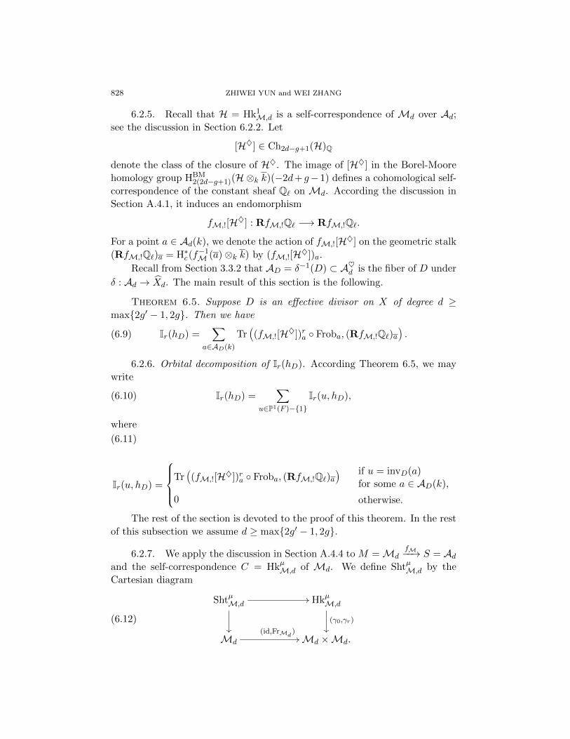
828 ZHIWEI YUN and WEI ZHANG
6.2.5. Recall that H = Hk1M,d is a self-correspondence of Md over Ad;
see the discussion in Section 6.2.2. Let
[H♦] ∈ Ch2d−g+1(H)Q
denote the class of the closure of H♦. The image of [H♦] in the Borel-Moore
homology group HBM2(2d−g+1)(H⊗k k)(−2d+ g−1) defines a cohomological self-
correspondence of the constant sheaf Q` on Md. According the discussion in
Section A.4.1, it induces an endomorphism
fM,![H♦] : RfM,!Q` −→ RfM,!Q`.
For a point a ∈ Ad(k), we denote the action of fM,![H♦] on the geometric stalk
(RfM,!Q`)a = H∗c(f−1M (a)⊗k k) by (fM,![H♦])a.
Recall from Section 3.3.2 that AD = δ−1(D) ⊂ A♥d is the fiber of D under
δ : Ad → “Xd. The main result of this section is the following.
Theorem 6.5. Suppose D is an effective divisor on X of degree d ≥max2g′ − 1, 2g. Then we have
(6.9) Ir(hD) =∑
a∈AD(k)
TrÄ(fM,![H♦])ra Froba, (RfM,!Q`)a
ä.
6.2.6. Orbital decomposition of Ir(hD). According Theorem 6.5, we may
write
(6.10) Ir(hD) =∑
u∈P1(F )−1Ir(u, hD),
where
Ir(u, hD) =
TrÄ(fM,![H♦])ra Froba, (RfM,!Q`)a
ä if u = invD(a)
for some a ∈ AD(k),
0 otherwise.
(6.11)
The rest of the section is devoted to the proof of this theorem. In the rest
of this subsection we assume d ≥ max2g′ − 1, 2g.
6.2.7. We apply the discussion in Section A.4.4 to M =MdfM−−→ S = Ad
and the self-correspondence C = HkµM,d of Md. We define ShtµM,d by the
Cartesian diagram
ShtµM,d//
HkµM,d
(γ0,γr)
Md
(id,FrMd)//Md ×Md.
(6.12)
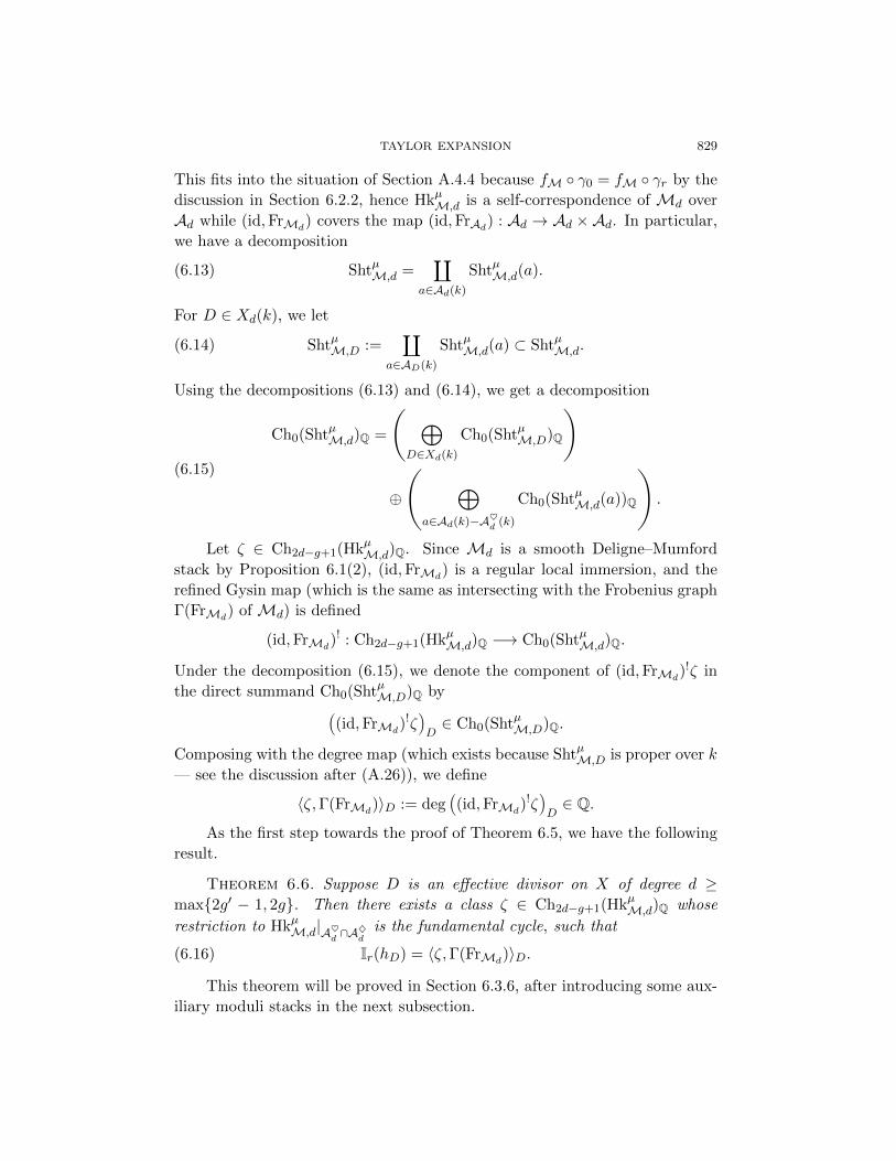
TAYLOR EXPANSION 829
This fits into the situation of Section A.4.4 because fM γ0 = fM γr by the
discussion in Section 6.2.2, hence HkµM,d is a self-correspondence of Md over
Ad while (id,FrMd) covers the map (id,FrAd) : Ad → Ad ×Ad. In particular,
we have a decomposition
(6.13) ShtµM,d =∐
a∈Ad(k)
ShtµM,d(a).
For D ∈ Xd(k), we let
(6.14) ShtµM,D :=∐
a∈AD(k)
ShtµM,d(a) ⊂ ShtµM,d.
Using the decompositions (6.13) and (6.14), we get a decomposition
Ch0(ShtµM,d)Q =
Ñ ⊕D∈Xd(k)
Ch0(ShtµM,D)Q
é⊕
Ö ⊕a∈Ad(k)−A♥
d(k)
Ch0(ShtµM,d(a))Q
è.
(6.15)
Let ζ ∈ Ch2d−g+1(HkµM,d)Q. Since Md is a smooth Deligne–Mumford
stack by Proposition 6.1(2), (id,FrMd) is a regular local immersion, and the
refined Gysin map (which is the same as intersecting with the Frobenius graph
Γ(FrMd) of Md) is defined
(id,FrMd)! : Ch2d−g+1(HkµM,d)Q −→ Ch0(ShtµM,d)Q.
Under the decomposition (6.15), we denote the component of (id,FrMd)!ζ in
the direct summand Ch0(ShtµM,D)Q byÄ(id,FrMd
)!ζäD∈ Ch0(ShtµM,D)Q.
Composing with the degree map (which exists because ShtµM,D is proper over k
— see the discussion after (A.26)), we define
〈ζ,Γ(FrMd)〉D := deg
Ä(id,FrMd
)!ζäD∈ Q.
As the first step towards the proof of Theorem 6.5, we have the following
result.
Theorem 6.6. Suppose D is an effective divisor on X of degree d ≥max2g′ − 1, 2g. Then there exists a class ζ ∈ Ch2d−g+1(HkµM,d)Q whose
restriction to HkµM,d|A♥d∩A♦
dis the fundamental cycle, such that
(6.16) Ir(hD) = 〈ζ,Γ(FrMd)〉D.
This theorem will be proved in Section 6.3.6, after introducing some aux-
iliary moduli stacks in the next subsection.

830 ZHIWEI YUN and WEI ZHANG
6.2.8. Proof of Theorem 6.5. Granting Theorem 6.6, we now prove Theo-
rem 6.5. Let ζ ∈ Ch2d−g+1(HkµM,d)Q be the class as in Theorem 6.6. By (6.14),
we have a decomposition
(6.17) Ch0(ShtµM,D)Q =⊕
a∈AD(k)
Ch0(ShtµM,d(a))Q.
We write〈ζ,Γ(FrMd
)〉D =∑
a∈AD(k)
〈ζ,Γ(FrMd)〉a
under the decomposition (6.17), where 〈ζ,Γ(FrMd)〉a is the degree ofÄ
(id,FrMd)!ζäa∈ Ch0(ShtµM,d(a))Q.
Combining this with Theorem 6.6 we get
(6.18) Ir(hD) =∑
a∈AD(k)
〈ζ,Γ(FrMd)〉a.
On the other hand, by Proposition A.12, for any a ∈ AD(k), we have
(6.19) 〈ζ,Γ(FrMd)〉a = Tr((fM,!cl(ζ))a Froba, (RfM,!Q`)a).
Here we are viewing the cycle class cl(ζ) ∈ HBM2(2d−g+1)(HkµM,d)(−2d + g − 1)
as a cohomological self-correspondence of the constant sheaf Q` onMd, which
induces an endomorphism
(6.20) fM,!cl(ζ) : RfM,!Q` −→ RfM,!Q`,
andan endomorphism(fM,!cl(ζ))a on the geometric stalk (RfM,!Q`)a. Since
we only care about the action of fM,!cl(ζ) on stalks in A♥d , only the restriction
ζ♥ := ζ|A♥d∈ Z2d−g+1(HkµM,d|A♥
d)Q matters. Combining (6.19) with (6.18),
we see that in order to prove (6.9), it suffices to show that fM,!cl(ζ♥) and
(fM,![H♦])r give the same endomorphism of the complex RfM,!Q`|A♥d
. This
is the following lemma, which is applicable because d ≥ 3g − 2 is implied by
d ≥ 2g′ − 1 = 4g − 3 (since g ≥ 1).
Lemma 6.7. Suppose d ≥ 3g−2 and ζ♥ ∈ Z2d−g+1(HkµM,d|A♥d
)Q. Suppose
the restriction of ζ♥ to HkµM,d|A♥d∩A♦
dis the fundamental cycle. Then the
endomorphism fM,!cl(ζ♥) of RfM,!Q`|A♥d
is equal to the r-th power of the
endomorphism fM,![H♦].
Proof. Let [H♦]r denote the r-th self-convolution of [H♦], which is a cycle
on the r-th self composition of H, and hence on HkµM,d by Lemma (6.2). We
have two cycle ζ♥ and (the restriction of) [H♦]r in Z2d−g+1(HkµM,d|A♥d
)Q. We
temporarily denoteMd|A♥d
byM♥d (although the same notation will be defined
in an a priori different way in Section 6.3). We need to show that they are in

TAYLOR EXPANSION 831
the same cycle class when projected toM♥d ×M♥d under (γ0, γr) : HkµM,d|A♥
d→
M♥d ×M♥d .
By assumption, when restricted to HkµM,d|A♥d∩A♦
d, both ζ♥ and [H♦]r are
the fundamental cycle. Therefore, the difference
(γ0, γr)∗(ζ♥ − [H♦]r) ∈ Z2d−g+1(M♥d ×M
♥d )Q
is supported on the image of HkµM,d|A♥d−A♦
din M♥d ×M
♥d , which is contained
in the image of HkµM,d − HkµM♦,d in Md ×Md. By Lemma 6.4(2), the latter
has dimension ≤ d+ 2g− 2. Since d > 3g− 3, we have d+ 2g− 2 < 2d− g+ 1,
therefore, (γ0, γr)∗(ζ♥ − [H♦]r) = 0 ∈ Z2d−g+1(M♥d ×M
♥d )Q, and the lemma
follows.
6.3. Auxiliary moduli stacks. The goal of this subsection is to prove The-
orem 6.6. Below we fix an integer d ≥ max2g′ − 1, 2g. In this subsection,
we will introduce moduli stacks Hk′rG,d and Hd that will fit into the following
commutative diagram:
(6.21)
HkµT ×HkµT
(γ0,γr)
(γ0,γr)
Πµ×Πµ// Hk′rG ×Hk′rG
(γ′0,γ′r)
(γ′0,γ′r)
Hk′rG,d
(γ′0,γ′r)
(←−ρ ′,−→ρ ′)oo
(BunT )2 × (BunT )2 Π×Π×Π×Π// (BunG)2 × (BunG)2 Hd ×Hd.
←→p 13×←→p 24oo
BunT × BunT
(id,Fr)
OO
(id,Fr)
OO
Π×Π// BunG × BunG
(id,Fr)
OO
(id,Fr)
OO
Hd
←→p =(←−p ,−→p )oo
(id,Fr)
OO
The maps in this diagram will be introduced later. The fiber products of the
three columns are
(6.22) ShtµT × ShtµTθµ×θµ−−−−→ Sht′rG × Sht′rG
(←−p ′,−→p ′)←−−−−− Sht′rG,d,
where Sht′rG,d is defined as the fiber product of the third column.
The fiber products of the three rows will be denoted
HkµM♥,d
(γ0,γr)
M♥d ×M♥d .
M♥d
(id,Fr)
OO(6.23)
These stacks will turn out to be the restrictions of Md and HkµM,d to A♥d , as
we will see in Lemmas 6.8(2) and 6.9.

832 ZHIWEI YUN and WEI ZHANG
6.3.1. In Section A.3 we discuss an abstract situation as in the above dia-
grams, which can be pictured using a subdivided octahedron. By Lemma A.9,
the fiber products of the two diagrams (6.22) and (6.23) are canonically iso-
morphic. We denote this stack by
ShtµM♥,d.
Below we will introduce Hd and Hk′rG,d.
6.3.2. We define ‹Hd to be the moduli stack whose S-points is the groupoid
of maps
φ : E → E ′,where E , E ′ are vector bundles over X×S of rank two, φ is an injective map of
OX×S-modules (so its cokernel has support finite over S), and prS∗ coker(φ) is
a locally free OS-module of rank d (where prS : X × S → S is the projection).
We have an action of PicX on ‹Hd by tensoring, and we form the quotient
Hd := ‹Hd/PicX .
Taking the map φ to its source and target gives two maps←−p ,−→p : Hd → BunG.
The map ←→p 13 ×←→p 24 that appears in (6.21) is the map
←→p 13 ×←→p 24 : Hd ×Hd−→BunG × BunG × BunG × BunG
(h, h′) 7−→ (←−p (h),←−p (h′),−→p (h),−→p (h′)).
On the other hand, we have the morphism Π : BunT → BunG sending Lto ν∗L; see Section 5.5.1. We form the following Cartesian diagram, and take
it as the definition of M♥d :
M♥d //
Hd
(←−p ,−→p )
BunT × BunTΠ×Π
// BunG × BunG.
(6.24)
Lemma 6.8.
(1) The morphisms ←−p ,−→p : Hd → BunG are representable and smooth of pure
relative dimension 2d. In particular, Hd is a smooth algebraic stack over
k of pure dimension 2d+ 3g − 3.
(2) There is a canonical open embeddingM♥d →Md whose image is f−1M (A♥d ).
(For the definition of A♥d , see Section 3.2.4.) In particular, M♥d is a
smooth Deligne–Mumford stack over k of pure dimension 2d− g + 1.
Proof. (1) Let Cohd0 be the stack classifying torsion coherent sheaves on
X of length d. By [18, (3.1)], Cohd0 is smooth of dimension 0. Consider
the map q : Hd → Cohd0 sending φ : E → E ′ to coker(φ). Then the map

TAYLOR EXPANSION 833
(←−p , q) : Hd → BunG × Cohd0 is a vector bundle of rank 2d whose fiber over
(E ,Q) is Ext1(Q, E). Therefore, ←−p is smooth of relative dimension 2d.
There is an involution δH on Hd sending φ : E → E ′ to φ∨ : E ′∨ → E∨. We
have ←−p δH = −→p because E ′∨ = E ′ canonically as G-bundles. Therefore, −→p is
also smooth of relative dimension 2d.
(2) By the diagram (6.24), M♥d classifies (L,L′, ψ) up to the action of
PicX , where L and L′ are as in the definition of ›Md, and ψ is an injective
OX -linear map ν∗L → ν∗L′.The discussion in Section 6.1.3 turns a point (L,L′, ψ : ν∗L → ν∗L′) ∈M♥d
into a point (L,L′, α : L → L′, β : L → σ∗L′) ∈ Md. The condition that ψ
be injective is precisely the condition that det(ψ) 6= 0, which is equivalent to
saying that fM(L,L′, ψ) ∈ A♥d , according to (6.1).
Proposition 6.1(2) shows that Md is a smooth Deligne–Mumford stack
over k of pure dimension 2d − g + 1, hence the same is true for its open
substack M♥d .
6.3.3. Recall the Hecke stacks HkrG and HkµT defined in (5.4) and (5.15).
Let Hkµ2,d be the moduli stack of commutative diagrams
E0//
φ0
E1//
φ1
· · · // Erφr
E ′0 // E ′1 // · · · // E ′r,
(6.25)
where both rows are points in Hkµ2 with the same image in Xr, and the vertical
maps φj are points in Hd (i.e., injective maps with colength d). Let
HkrG,d = Hkµ2,d/PicX ,
where PicX simultaneously acts on all Ei and E ′i by tensor product. The same
argument of Lemma 5.5 shows that HkrG,d is independent of µ.
There are natural maps HkrG → Xr and HkrG,d → Xr. We define
Hk′rG = HkrG ×Xr X ′r; Hk′rG,d := HkrG,d ×Xr X ′r.
The map HkµT → HkrG given by Ei = ν∗Li induces a map
Πµ : HkµT −→ Hk′rG.
We have two maps
←−ρ ,−→ρ : HkrG,d −→ HkrG
sending the diagram (6.25) to its top and bottom row. We denote their base
change to X ′r by←−ρ ′,−→ρ ′ : Hk′rG,d −→ Hk′rG.

834 ZHIWEI YUN and WEI ZHANG
We define HkµM♥,d by the following Cartesian diagram:
HkµM♥,d//
Hk′rG,d
(←−ρ ′,−→ρ ′)
HkµT ×HkµTΠµ×Πµ
// Hk′rG ×Hk′rG.
(6.26)
The same argument of Lemma 6.8(2) shows the following result. Recall
that the stack HkµM,d is defined in Section 6.2.1.
Lemma 6.9. There is a canonical isomorphism between HkµM♥,d and the
preimage of A♥d under the natural map fM γ0 : HkµM,d → Ad.
6.3.4. We have a map
s : HkrG,d −→ Xd ×Xr
that sends a diagram (6.25) to (D;x1, . . . , xr), where D is the divisor of det(φi)
for all i. Let (Xd×Xr) ⊂ Xd×Xr be the open subscheme consisting of those
(D;x1, . . . , xr) where xi is disjoint from the support of D for all i. Let
Hkr,G,d = s−1((Xd ×Xr))
be an open substack of HkrG,d. Let Hk′r,G,d ⊂ Hk′rG,d and Hkµ,M♥,d ⊂ HkµM♥,d be
the preimages of Hkr,G,d.
Lemma 6.10.
(1) The stacks Hkr,G,d and Hk′r,G,d are smooth of pure dimension 2d+2r+3g−3.
(2) The dimensions of all geometric fibers of s are d+r+3g−3. In particular,
dim HkrG,d = dim Hk′rG,d = 2d+ 2r + 3g − 3.
(3) Recall that HkµM♦,d is the restriction HkµM,d|A♦d
, where A♦d ⊂ Ad is de-
fined in Section 6.2.4. Suppose d ≥ max2g′ − 1, 2g. Let Hkµ,M♦,d be the
intersection of HkµM♦,d with Hkµ,M♥,d inside HkµM,d. Then
dim(HkµM♦,d −Hkµ,M♦,d) < 2d− g + 1 = dim HkµM♦,d.
The proof of this lemma will be postponed to Sections 6.4.1–6.4.3.
Lemma 6.11. Suppose d ≥ max2g′ − 1, 2g.(1) The diagram (6.26) satisfies the conditions in Section A.2.8. In particular,
the refined Gysin map
(Πµ ×Πµ)! : Ch∗(Hk′rG,d)Q −→ Ch∗−2(2g−2+r)(HkµM♥,d)Q
is defined.

TAYLOR EXPANSION 835
(2) Let
(6.27) ζ♥ = (Πµ ×Πµ)![Hk′rG,d] ∈ Ch2d−g+1(HkµM♥,d)Q.
Then the restriction of ζ♥ to HkµM♥,d|A♦d ∩A♥d is the fundamental cycle.
Proof. (1) We first check that HkµM♥,d admits a finite flat presentation.
The map γ0 : HkµM♥,d → M♥d is schematic, so it suffices to check that M♥d
or Md admits a finite flat presentation. In the proof of Proposition 6.1(1) we
constructed a proper and schematic map h :Md → JdX′×PrymX′/X ; see (6.4).
Since JdX′ is a scheme and PrymX′/X is the quotient of the usual Prym variety
by the trivial action of µ2, JdX′ × PrymX′/X admits a finite flat presentation,
hence so do Md and HkµM♥,d.
Next we verify condition (2) of Section A.2.8. Extending k if necessary,
we may choose a point y ∈ X(k) that is split into y′, y′′ ∈ X ′(k). Let BunG(y)
be the moduli stack of G-torsors over X with a Borel reduction at y. Let
Hk′rG(y) = Hk′rG ×BunG BunG(y) where the map Hk′rG → BunG sends (Ei;xi; fi)to E0. We may lift the morphism Πµ to a morphism
Πµ(y) : HkµT −→ Hk′rG(y),
where the Borel reduction of E0 = ν∗L0 at y (i.e., a line in the stalk E0,y) is
given by the stalk of L0 at y′. The projection p : Hk′rG(y) → Hk′rG is smooth,
and Πµ = p Πµ(y). So to check condition (2) of Section A.2.8, it suffices to
show that Πµ(y) is a regular local immersion.
We will show by tangential calculations that Hk′rG(y) is a Deligne–Mumford
stack in a neighborhood of the image of Πµ(y), and the tangent map of Πµ(y)
is injective. For this it suffices to make tangential calculations at geometric
points of HkµT and its image in Hk′rG(y). We identify HkµT with BunT ×X ′r as
in Section 5.4.4. Fix a geometric point (L;x′) ∈ PicX′(K)×X ′(K)r. For nota-
tional simplicity, we base change the situation from k to K without changing
notation. So X means X ⊗k K, etc.
The relative tangent space of HkµT → X ′r at (L;x′) is H1(X,OX′/OX).
The relative tangent complex of Hk′rG(y)→ X ′r at
Πµ(y)(L;x′) = (ν∗L −→ ν∗L(x′1) −→ · · · ;Ly′)
is
H∗(X,Adx′,y(ν∗L))[1],
where Adx′,y(ν∗L) = Endx
′,y(ν∗L)/OX · id and Endx′,y(ν∗L) is the endomor-
phism sheaf of the chain of vector bundles ν∗L → ν∗L(x′1) → · · · preserving

836 ZHIWEI YUN and WEI ZHANG
the line Ly′ of the stalk (ν∗L)y. Note that
Endx′,y(ν∗L) ⊂ Endy(ν∗L) = ν∗Hom(L ⊕ (σ∗L)(y′′),L)
= ν∗OX′ ⊕ ν∗(L ⊗ σ∗L−1(−y′′)).(6.28)
We also have a natural inclusion
γ : ν∗OX′ → Endx′,y(ν∗L)
identifying the left-hand side as those endomorphisms of ν∗L that are OX′-linear. Now γ(ν∗OX′) maps isomorphically to ν∗OX′ on the right-hand side
of (6.28). Combining these we get a canonical decomposition Endx′,y(ν∗L) =
ν∗OX′ ⊕ K for some line bundle K on X with deg(K) < 0. Consequently, we
have a canonical decomposition
(6.29) Adx′,y(ν∗L) = OX′/OX ⊕K.
In particular, H0(X,Adx′,y(ν∗L)) = H0(X,OX′/OX) = 0. This shows that
Hk′rG(y) is a Deligne–Mumford stack in a neighborhood of Πµ(y)(L;x′).
The tangent map of Πµ(y) is the map
H1(X,OX′/OX) −→ H1(X,Adx′,y(ν∗L))
induced by γ, hence it corresponds to the inclusion of the first factor in the
decomposition (6.29). In particular, the tangent map of Πµ(y) is injective. This
finishes the verification of all conditions in Section A.2.8 for the diagram (6.26).
(2) Let Hkµ,M♥,d be the preimage of Hk′r,G,d. By Lemma 6.10(1), Hk′r,G,d is
smooth of dimension 2d+2r+3g−3. On the other hand, by Lemma 6.4, HkµM♦,dhas dimension 2d−g+1. Combining these facts, we see that Hkµ,M♥,d∩HkµM♦,dhas the expected dimension in the Cartesian diagram (6.26). This implies that
ζ♥|Hkµ,M♥,d
∩HkµM♦,d
is the fundamental cycle. By Lemma 6.10(3), HkµM♦,d −
Hkµ,M♥,d has lower dimension than HkµM♦,d, therefore, ζ♥|HkµM♦,d
must be the
fundamental cycle.
6.3.5. There are r + 1 maps γi (0 ≤ i ≤ r) from the diagram (6.26) to
(6.24): it sends the diagram (6.25) to its i-th column, etc. In particular, we
have maps γi : HkrG,d → Hd and γ′i : Hk′rG,d → Hd. The maps γ′0 and γ′r appear
in the diagram (6.21).
We define the stack ShtrG,d by the following Cartesian diagram:
ShtrG,d
// HkrG,d
(γ0,γr)
Hd
(id,Fr)// Hd ×Hd.
(6.30)

TAYLOR EXPANSION 837
Similarly, we define Sht′rG,d as the fiber product of the third column of (6.21):
Sht′rG,d
// Hk′rG,d
(γ′0,γ′r)
Hd
(id,Fr)// Hd ×Hd.
(6.31)
We have Sht′rG,d∼= ShtrG,d ×Xr X ′r.
Lemma 6.12. There are canonical isomorphisms of stacks
ShtrG,d∼=
∐D∈Xd(k)
ShtrG(hD),
Sht′rG,d∼=
∐D∈Xd(k)
Sht′rG(hD).
For the definitions of ShtrG(hD) and Sht′rG(hD), see Sections 5.3.1 and 5.3.2.
Proof. From the definitions, (γ0, γr) factors through the map HkrG,d →Hd ×Xd Hd. On the other hand, (id,Fr) : Hd → Hd × Hd covers the similar
map (id,Fr) : Xd → Xd ×Xd. By the discussion in Section A.4.5, we have a
decomposition
ShtrG,d =∐
D∈Xd(k)
ShtrG,D.
Let HD and HkrG,D be the fibers of Hd and HkrG,d over D. Then the D-com-
ponent ShtrG,D of ShtrG,d fits into a Cartesian diagram
ShtrG,D //
HkrG,D
(γ0,γr)
HD(id,Fr)// HD ×HD.
(6.32)
Comparing this with the definition in Section 5.3.1, we see that ShtrG,D∼=
ShtrG(hD). The statement for Sht′rG,d follows from the statement for ShtrG,d by
base change to X ′r.
Corollary 6.13. Let D ∈ Xd(k) (i.e., an effective divisor on X of de-
gree d). Recall the stack ShtµM,d defined in (6.12) and ShtµM♥,d defined in
Section 6.3.1. Then ShtµM♥,d is canonically isomorphic to the restriction of
ShtµM,d to A♥d (k) ⊂ Ad(k).
Moreover, there is a canonical decomposition
ShtµM♥,d =∐
D∈Xd(k)
ShtµM,D,

838 ZHIWEI YUN and WEI ZHANG
where ShtµM,D is defined in (6.14). In particular, we have a Cartesian diagram
(6.33) ShtµM,D
// Sht′rG(hD)
(←−p ′,−→p ′)
ShtµT × ShtµTθµ×θµ
// Sht′rG × Sht′rG.
Proof. Note that ShtµM♥,d is defined as a fiber product in two ways: one as
the fiber product of (6.22) and the other as the fiber product of (6.23). Using
the first point of view and the decomposition of Sht′rG,d given by Lemma 6.12,
we get a decomposition of ShtµM♥,d =∐D∈Xd(k) ShtµM♥,D, where ShtµM♥,D is
by definition the stack to put in the upper left corner of (6.33) to make the
diagram Cartesian.
On the other hand, using the second point of view of ShtµM♥,d as the
fiber product of (6.23), and using the fact that HkµM♥,d is the restriction
of HkµM,d over A♥d by Lemma 6.9, we see that ShtµM♥,d is the restriction of
ShtµM,d over A♥d by comparing (6.23) and (6.12). By (6.13) and (6.14), and
the fact that A♥d (k) =∐D∈Xd(k)AD(k), we get a decomposition ShtµM♥,d =∐
D∈Xd(k) ShtµM,D. Therefore, both ShtµM♥,D and ShtµM,D are the fiber of the
map ShtµM,d → Ad → “Xd over D, and they are canonically isomorphic. Hence
we may replace the upper left corner of (6.33) by ShtµM♥,D, and the new dia-
gram is Cartesian by definition.
Lemma 6.14.
(1) The diagram (6.31) satisfies the conditions in Section A.2.10. In particu-
lar, the refined Gysin map
(id,FrHd)! : Ch∗(Hk′rG,d)Q −→ Ch∗−dimHd(Sht′rG,d)Q
is defined.
(2) We have
[Sht′rG,d] = (id,FrHd)![Hk′rG,d] ∈ Ch2r(Sht′rG,d).
Proof. (1) Since ←−p : ShtrG(hD) → ShtrG is representable by Lemma 5.8,
ShtrG(hD) is also a Deligne–Mumford stack. Since ShtrG,d is the disjoint union of
ShtrG(hD) by Lemma 6.12, ShtrG,d is Deligne–Mumford, hence so is Sht′rG,d. The
map γ′0 : Hk′rG,d → Hd is representable because its fibers are closed subschemes
of iterated Quot schemes (fixing E0 → E ′0, building Ei and E ′i step by step and
imposing commutativity of the maps). Therefore, (γ′0, γ′r) is also representable.
This verifies condition (1) in Section A.2.10.
Since Hd is smooth by Lemma 6.8, the normal cone stack of the map
(id,FrHd) : Hd → Hd ×Hd is the vector bundle stack Fr∗ THd, the Frobenius
TAYLOR EXPANSION 839
pullback of the tangent bundle stack of Hd. Therefore, (id,FrHd) satisfies
condition (2) in Section A.2.10. It also satisfies condition (3) of Section A.2.10
by the discussion in Remark A.7.
Finally the dimension condition (4) in Section A.2.10 for Hk′rG,d and Sht′rG,d=∐D Sht′rG(hD) follows from Lemma 6.10(2) and Lemma 5.9. We have verified
all conditions in Section A.2.10.
(2) Take the open substack Hk′r,G,d ⊂ Hk′rG,d as in Lemma 6.10. Then Hk′r,G,dis smooth of pure dimension 2d+ 2r + 3g − 3. According to Lemma 6.12, the
corresponding open part Sht′r,G,d is the disjoint union of Sht′r,G (hD), where
Sht′r,G (hD) = Sht′rG(hD)|(X′−ν−1(D))r .
It is easy to see that both projections Sht′r,G (hD) → Sht′rG are etale, hence
Sht′r,G (hD) is smooth of dimension 2r = dim Hk′r,G,d − codim(id,FrHd), the ex-
pected dimension. This implies that if we replace Hk′rG,d with Hk′r,G,d, and
replace Sht′rG,d with Sht′r,G,d in the diagram (6.31), it becomes a complete inter-
section diagram. Therefore, (id,FrHd)![Hk′rG,d] is the fundamental cycle when
restricted to Sht′r,G,d. Since Sht′rG,d − Sht′r,G,d has lower dimension than 2r by
Lemma 5.9, we see that (id,FrHd)![Hk′rG,d] must be equal to the fundamental
cycle over the whole Sht′rG,d.
6.3.6. Proof of Theorem 6.6. Consider the diagram (6.33). Since ShtµTis a proper Deligne–Mumford stack over k and the map (←−p ′,−→p ′) is proper
and representable, ShtµM,D is also a proper Deligne–Mumford stack over k. A
simple manipulation using the functoriality of Gysin maps gives
Ir(hD) = 〈θµ∗ [ShtµT ], hD ∗ θµ∗ [ShtµT ]〉Sht′rG= deg
Ä(θµ × θµ)![Sht′rG(hD)]
ä.
Here (θµ× θµ)! : Ch2r(Sht′rG(hD))Q → Ch0(ShtµM,D)Q is the refined Gysin map
attached to the map θµ × θµ. By Corollary 6.13, (θµ × θµ)![Sht′rG(hD)] is the
D-component of the 0-cycle
(θµ × θµ)![Sht′rG,d] ∈ Ch0(ShtµM♥,d)Q =⊕
D∈Xd(k)
Ch0(ShtµM,D)Q.
Therefore, to prove (6.16) simultaneously for all D of degree d, it suffices to
find a cycle class ζ♥ ∈ Ch2d−g+1(HkµM♥,d)Q whose restriction to HkµM♥,d ∩HkµM♦,d = HkµM,d|A♥
d∩A♦
dis the fundamental class, and that
(6.34) (θµ × θµ)![Sht′rG,d] = (id,FrM♥d
)!ζ♥ ∈ Ch0(ShtµM♥,d)Q.
The statement of Theorem 6.6 asks for a cycle ζ on HkµM,d, but we may extend
the above ζ♥ arbitrarily to a (2d− g + 1)-cycle in HkµM,d.
To prove (6.34), we would like to apply Theorem A.10 to the situation of
(6.21). We check the following assumptions:

840 ZHIWEI YUN and WEI ZHANG
(1) The smoothness of BunT and BunG is well known. The smoothness of Hk′rGand HkµT follow from Remark 5.2 and Section 5.4.4. Finally, by Lemma 6.8,
Hd is smooth of pure dimension 2d+ 3g − 3. This checks the smoothness
of all members in (6.21) except B = Hk′rG,d.
(2) By Corollary 5.7, ShtrG, and hence Sht′rG is smooth of pure dimension 2r;
by Lemma 5.13, ShtµT is smooth of pure dimension r. By Lemma 6.8,M♥dis smooth of pure dimension 2d − g + 1. All of them have the dimension
expected from the Cartesian diagrams defining them.
(3) The diagram (6.31) satisfies the conditions in Section A.2.10 by Lemma
6.14. The diagram (6.26) satisfies the conditions in Section A.2.8 by
Lemma 6.11.
(4) We check that the Cartesian diagram formed by (6.23), or rather (6.12),
satisfies the conditions in Section A.2.8. The map ShtµM,d →Md is repre-
sentable because HkµM,d → Md ×Md is. In the proof of Lemma 6.11(1)
we have proved that Md admits a finite flat presentation, hence so does
ShtµM,d. This verifies the first condition in Section A.2.8. Since Md is
a smooth Deligne–Mumford stack by Lemma 6.1(2), (id,FrMd) : Md →
Md × Md is a regular local immersion, which verifies condition (2) of
Section A.2.8.
Finally we consider the Cartesian diagram formed by (6.22) (or equiv-
alently, the disjoint union of the diagrams (6.33) for all D ∈ Xd(k)). We
have already showed above that ShtµM,d admits a finite flat presentation.
All members in these diagrams are Deligne–Mumford stacks, and ShtµTand Sht′rG are smooth Deligne–Mumford stacks by Lemma 5.13 and Corol-
lary 5.7. Hence the map θµ× θµ satisfies condition (2) of Section A.2.8 by
Remark A.4.
Now we can apply Theorem A.10 to the situation (6.21). Let
ζ♥ = (Πµ ×Πµ)![Hk′rG,d] ∈ Ch2d−g+1(HkµM♥,d)Q
as defined in (6.27). Then the restriction of ζ♥ to HkµM,d|A♦d∩A♥
dis the funda-
mental cycle by Lemma 6.11(2). Finally,
(id,FrM♥d
)!ζ♥ = (id,FrM♥d
)!(Πµ ×Πµ)![Hk′rG,d]
= (θµ × θµ)!(id,FrHd)![Hk′rG,d] (Theorem A.10)
= (θµ × θµ)![Sht′rG,d] (Lemma 6.14(2)),
which is (6.34). This finishes the proof of (6.16).
6.4. Some dimension calculation. In this subsection, we give the proofs of
several lemmas that we stated previously concerning the dimensions of certain
moduli stacks.

TAYLOR EXPANSION 841
6.4.1. Proof of Lemma 6.10(1). In the diagram (6.25), when the divisors
of the φi are disjoint from the divisors of the horizontal maps — namely, the
xi’s — the diagram is uniquely determined by its left column φ0 : E0 → E ′0 and
top row. Therefore, we have
Hkr,G,d = (Hd ×BunG HkrG)|(Xd×Xr) .
Since Hd is smooth of pure dimension 2d+ 3g− 3 by Lemma 6.8, and the map
p0 : HkrG → BunG is smooth of relative dimension 2r, we see that Hd×BunGHkrGis smooth of pure dimension 2d+ 2r + 3g − 3.
6.4.2. Proof of Lemma 6.10(2). Over (Xd × Xr), we have dim Hkr,G,d =
2d+2r+3g−3, therefore, the generic fiber of s has dimension d+r+3g−3. By
the semicontinuity of fiber dimensions, it suffices to show that the geometric
fibers of s have dimension ≤ d + r + 3g − 3. We will actually show that the
geometric fibers of the map (s, p0) : HkrG,d → Xd × Xr × BunG sending the
diagram (6.25) to (D;xi; E ′r) have dimension ≤ d+ r.
We present HkrG,d as the quotient of Hkµ2,d/PicX with µ = µr+. Therefore,
a point in HkrG,d is a diagram of the form (6.25) with all arrows fi, f′i pointing
to the right.
Let (D;x = (xi)) ∈ Xd × Xr and E ′r ∈ BunG be geometric points. For
notational simplicity, we base change the whole situation to the field of defini-
tion of this point without changing notation. Let HD,x,E ′r be the fiber of (s, p0)
over (D;xi; E ′r). We consider the scheme H ′ = H ′D,x,E ′r classifying commutative
diagrams
E0f1//
φ0
E1f2// · · ·
fr// Er
φr
E ′0f ′1// E ′1
f ′2// · · ·
f ′r// E ′r,
(6.35)
where div(detφ0) = D = div(detφr) and div(det fi) = xi = div(det f ′i). The
only difference between H ′ and HD,x,E ′r is that we do not require the maps φifor 1 ≤ i ≤ r − 1 to exist. (They are unique if they exist.) There is a natural
embedding HD,x,E ′r → H ′, and it suffices to show that dim(H ′) ≤ d + r. We
isolate this part of the argument into a separate lemma below, because it will
be used in another proof. This finishes the proof of Lemma 6.10(2).
Lemma 6.15. Consider the scheme H ′ = H ′D,x,E ′r introduced in the proof
of Lemma 6.10(2). We have dimH ′ = d+ r.
Proof. We only give the argument for the essential case where all xi are
equal to the same point x and D = dx. The general case can be reduced to this
case by factorizing H ′ into a product indexed by points that appear in |D| ∪x1, . . . , xr. Let Gr1r,d be the iterated version of the affine Schubert variety

842 ZHIWEI YUN and WEI ZHANG
classifying chains of lattices Λ0 ⊂ Λ1 ⊂ Λ2 ⊂ · · · ⊂ Λr ⊂ Λ′r = O2x in F 2
x where
all inclusions have colength 1 except for the last one, which has colength d.
Similarly, let Grd,1r be the iterated affine Schubert variety classifying chains
of lattices Λ0 ⊂ Λ′0 ⊂ Λ′1 ⊂ · · · ⊂ Λ′r = O2x in F 2
x where the first inclusion has
colength d and all other inclusions have colength 1. Let Grd+r ⊂ GrG,x be the
affine Schubert variety classifying Ox-lattices Λ ⊂ O2x with colength d+ r. We
have natural maps π : Gr1r,d → Grd+r and π′ : Grd,1r → Grd+r sending the
lattice chains to Λ0. By the definition of H ′, after choosing a trivialization of
E ′r in the formal neighborhood of x, we have an isomorphism
(6.36) H ′ ∼= Gr1r,d ×Grd+r Grd,1r .
Since π and π′ are surjective, therefore, dimH ′ ≥ dim Grd+r = d+ r.
Now we show dimH ′ ≤ d + r. Since the natural projections Gr1d+r →Gr1r,d and Gr1d+r → Grd,1r are surjective, it suffices to show that
dim(Gr1d+r ×Grd+r Gr1d+r) ≤ d+ r.
In other words, letting m = d+ r, we have to show that πm : Gr1m → Grm is a
semismall map. This is a very special case of the semismallness of convolution
maps in the geometric Satake equivalence, and we shall give a direct argument.
The scheme Grm is stratified into Y im (0 ≤ i ≤ [m/2]), where Y i
m classifies those
Λ ⊂ O2x such that O2
x/Λ∼= Ox/$i
x ⊕Ox/$m−ix . We may identify Y i
m with the
open subscheme Y 0m−2i ⊂ Grm−2i by sending Λ ∈ Y i
m to $−ix Λ ⊂ O2x, hence
dimY im = m − 2i and codimGrmY
im = i. We need to show that for Λ ∈ Yi,
dimπ−1m (Λ) ≤ i. We do this by induction on m. By definition, π−1
m (Λ) classifies
chains Λ = Λ0 ⊂ Λ1 ⊂ · · · ⊂ Λm = O2x, each step of which has colength one.
For i = 0, such a chain is unique. For i > 0, the choices of Λ1 are parametrized
by P1, and the map ρ : π−1m (Λ)→ P1 recording Λ1 has fibers π−1
m−1(Λ1). Either
O2x/Λ1
∼= Ox/$i−1x ⊕Ox/$m−i
x , in which case dim ρ−1(Λ1) = dimπ−1m−1(Λ1) ≤
i−1 by inductive hypothesis, orO2x/Λ1
∼= Ox/$ix⊕Ox/$m−i−1
x (which happens
for exactly one Λ1), in which case dim ρ−1(Λ1) = dimπ−1m−1(Λ1) ≤ i. These
imply that dimπ−1m (Λ) ≤ i. The lemma is proved.
6.4.3. Proof of Lemma 6.10(3). We denote HkµM♦,d−Hkµ,M♦,d by ∂HkµM♦,d.
By Lemmas 6.2 and 6.3, HkµM♦,d∼= “X ′d×PicdX
Br,d, where Br,d classifies (r+1)-
triples of divisors (D0, D1, . . . , Dr) of degree d on X ′, such that for each
1 ≤ i ≤ r, Di is obtained from Di−1 by changing some point x′i ∈ Di−1 to
σ(x′i). In particular, all Di have the same image Db := π(Di) ∈ Xd. We
denote a point in HkµM♦,d by z = (L, α,D0, . . . , Dr) ∈ “X ′d ×PicdXBr,d, where
(L, α) ∈ “X ′d denotes a line bundle L on X ′ and a section α of it, together
with an isomorphism Nm(L) ∼= OX(Db). Therefore, both Nm(α) and 1 give
sections of OX(Db). The image of z under HkµM♦,d → Adδ−→ “Xd is the pair
(OX(Db),Nm(α)− 1). Therefore, z ∈ ∂HkµM♦,d if and only if div(Nm(α)− 1)

TAYLOR EXPANSION 843
contains π(x′i) for some 1 ≤ i ≤ r; Nm(α) = 1 is allowed. Since x′i ∈ Di−1,
we have π(x′i) ∈ π(Di−1) = Db, therefore, π(x′i) also appears in the divisor of
Nm(α). So we have two cases: either α = 0 or div(Nm(α)) shares a common
point with Db.
In the former case, z is contained in PicdX′ ×PicdXBr,d that has dimension
g − 1 + d < 2d− g + 1 since d ≥ 2g.
In the latter case, the image of z in Ad lies in the subscheme Cd ⊂ Xd
×PicdXXd consisting of triples (D1, D2, γ : O(D1) ∼= O(D2)) such that the divi-
sors D1 and D2 have a common point. There is a surjection X× (Xd−1×Picd−1X
Xd−1) → Cd, which implies that dim Cd ≤ 1 + 2(d − 1) − g + 1 = 2d − g.
Here we are using the fact that d − 1 ≥ 2g − 1 to compute the dimension
of Xd−1 ×Picd−1X
Xd−1. The conclusion is that in the latter case, z lies in
the preimage of Cd in HkµM♦,d, which has dimension equal to dim Cd (be-
cause HkµM,d → Ad is finite when restricted to Cd ⊂ Xd ×PicdXXd), which
is ≤ 2d− g < 2d− g + 1.
Combining the two cases we conclude that dim ∂HkµM♦,d < 2d − g + 1 =
dim HkµM♦,d.
6.4.4. Proof of Lemma 5.9. Let x = (x1, . . . , xr) ∈ Xr be a geometric
point. Let ShtrG(hD)x be the fiber of ShtrG(hD) over x. When x is disjoint
from |D|, then ←−p : ShtrG(hD)x → ShtrG,x is etale, and hence in this case
dim ShtrG(hD)x = r. By semicontinuity of fiber dimensions, it remains to show
that dim ShtrG(hD)x ≤ r for all geometric points x over closed points of Xr.
To simplify notation we assume xi ∈ X(k). The general case can be argued
similarly.
We use the same notation as in Section 6.4.2. In particular, we will use
HkrG,d and think of it as Hkµ2,d/PicX with µ = µr+. Let HD be the fiber over
D of Hd → Xd sending (φ : E → E ′) to the divisor of det(φ). Let HkrD,x be the
fiber of s : HkrG,d → Xd ×Xr over (D;x).
Taking the fiber of the diagram (6.32) over x we get a Cartesian diagram
ShtrG(hD)x
// HkrD,x
(p0,pr)
HD(id,Fr)
// HD ×HD.
(6.37)
For each divisor D′ ≤ D such that D − D′ has even coefficients, we have a
closed embedding HD′ → HD sending (φ : E → E ′) ∈ HD′ to E φ−→ E ′ →E ′(1
2(D−D′)). Let HD,≤D′ be the image of this embedding. Also let HD,D′ =
HD,≤D′ − ∪D′′<D′HD,≤D′′ . Then HD,D′ give a stratification of HD indexed
by divisors D′ ≤ D such that D − D′ is even. We may restrict the diagram

844 ZHIWEI YUN and WEI ZHANG
(6.37) to HD,D′ ×HD,D′ → HD ×HD and get a Cartesian diagram
ShtrG(hD)D′,x
// HkrD,D′,x
(p0,pr)
HD,D′(id,Fr)
// HD,D′ ×HD,D′ .
(6.38)
We will show that dim ShtrG(hD)D′,x ≤ r for each D′ ≤ D and D −D′ even.
The embedding HD′ → HD above restricts to an isomorphism HD′,D′∼=
HD,D′ . Similarly, we have an isomorphism HkrD′,D′,x∼= HkrD,D′,x sending a
diagram of the form (6.25) to the diagram of the same shape with each E ′ichanged to E ′(1
2(D −D′)). Therefore, we have ShtG(hD′)D′,x ∼= ShtG(hD)D′,x,
and it suffices to show that the open stratum ShtG(hD)D,x has dimension at
most r. This way we reduce to treating the case D′ = D.
Let ‹D = D+x = D+x1 +· · ·+xr ∈ Xd+r be the effective divisor of degree
d+r. Let BunG,D
be the moduli stack of G bundles with a trivialization over ‹D.
A point of BunG,D
is a pair (E ′, τ : E ′D∼= O2
D) (where E ′ is a vector bundle of
rank two over X) up to the action of PicX(‹D) (line bundles with a trivialization
over ‹D). There is a map h : BunG,D→ HD,D sending (E ′, τ) to (φ : E → E ′),
where E is the preimage of the first copy of OD under the surjective map
E ′ E ′Dτ−→ O2
D O2
D. Let BD ⊂ ResODk G = PGL2(OD) be the subgroup
stabilizing the first copy of O2D, and let ‹BD ⊂ Res
OD
k G = PGL2(OD
) be the
preimage of BD. Then h is a ‹BD-torsor. In particular, HD,D is smooth, and
the map h is also smooth. Since smooth maps have sections etale locally, we
may choose an etale surjective map ω : Y → HD,D and a map s : Y → BunG,D
such that hs = ω.
Let W = HkrD,D,x ×HD,D Y (using the projection γr : HkrD,D,x → HD,D).
We claim that the projection W → Y is in fact a trivial fibration. In fact,
let T be the moduli space of diagrams of the form (6.25) with Er = O2X ,
Er = OX(−D) ⊕ OX , and φr being the obvious embedding Er → E ′r. In
such a diagram all Ei and E ′i contain E ′r(−‹D). Therefore, it contains the same
amount of information as the diagram formed by the torsion sheaves Ei/E ′r(−‹D)
and E ′i/E ′r(−‹D). For a point y ∈ Y with image (φr : Er → E ′r) ∈ HD,D,
s(y) ∈ BunG,D
gives a trivialization of E ′r|D. Therefore, completing φr into
a diagram of the form (6.25) is the same as completing the standard point
(Er = OX(−D) ⊕ OX → O2X) ∈ HD,D into such a diagram. This shows that

TAYLOR EXPANSION 845
W ∼= Y × T . We have a diagram
U
u
// W
w
∼// Y × T ω×id
// HD,D × T
ShtrG(hD)D,x //
HkrD,D,x
(γ0,γr)
HD,D(id,Fr)
// HD,D ×HD,D,
where U is defined so that the top square is Cartesian. The outer Cartesian
diagram fits into the situation of [15, Lemme 2.13], and we have used the same
notation as in loc. cit, except that we take Z = HD,D. Applying loc. cit.,
we conclude that the map U → T is etale. Since w : W → HkrD,D,x is etale
surjective, so is u : U → ShtrG(hD)D,x. Therefore, ShtrG(hD)D,x is etale locally
isomorphic to T and, in particular, they have the same dimension.
It remains to show that dimT ≤ r. Recall the moduli space H ′ = H ′D,x,E ′rintroduced in the proof of Lemma 6.10(2) classifying diagrams of the form
(6.35). Here we fix E ′r = O2X . Let T ′ be subscheme of H ′ consisting of diagrams
of the form (6.35) where (φr : Er → E ′r) is fixed to be (Er = OX(−D) ⊕ OX→ O2
X). Then we have a natural embedding T → T ′, and it suffices to show
that dimT ′ ≤ r. Again we treat only the case where D and x are both sup-
ported at a single point x ∈ X. The general case easily reduces to this by
factorizing T ′ into a product indexed by points in |D| ∪ x1, . . . , xr.Let Grd⊂GrG,x be the affine Schubert variety classifying lattices Λ⊂O2
x
of colength d. Let Gr♥d ⊂ Grd be the open Schubert stratum consisting of
lattices Λ ⊂ O2x such that O2
x/Λ∼= Ox/$d
x. (Here $x is a uniformizer at x.)
We have a natural projection ρ : H ′ → Grd sending the diagram (6.35) to
Λ := Er|SpecOx → E ′r|SpecOx = O2x. Then T ′ is the fiber of ρ at the point
Λ = $dxOx ⊕ Ox. Let H♥ = ρ−1(Gr♥d ). There is a natural action of the
positive loop group L+xG on both H ′ and Grd making ρ equivariant under
these actions. Since the action of L+xG on Gr♥d is transitive, all fibers of ρ over
points of Gr♥d have the same dimension, i.e.,
(6.39) dimT ′ = dimH♥ − dim Gr♥d = dimH♥ − d.
By Lemma 6.15, dimH ′ = d + r. Therefore, dimH♥ = d + r and dimT ′ ≤ r
by (6.39). We are done.
7. Cohomological spectral decomposition
In this section, we give a decomposition of the cohomology of ShtrG under
the action of the Hecke algebra H , generalizing the classical spectral decom-
position for the space of automorphic forms. The main result is Theorem 7.14,

846 ZHIWEI YUN and WEI ZHANG
which shows that H2rc (Shtr
G,k,Q`) is an orthogonal direct sum of an Eisenstein
part and finitely many (generalized) Hecke eigenspaces. We then use a variant
of such a decomposition for Sht′rG to make a decomposition for the Heegner-
Drinfeld cycle.
7.1. Cohomology of the moduli stack of Shtukas.
7.1.1. Truncation of BunG by index of instability. For a rank two vector
bundle E over X, we define its index of instability to be
inst(E) := max2 degL − deg E,
where L runs over the line subbundle of E . When inst(E) > 0, E is called
unstable, in which case there is a unique line subbundle L ⊂ E such that
degL > 12 deg E . We call this line subbundle the maximal line subbundle of E .
Note that there is a constant c(g) depending only on the genus g of X such
that inst(E) ≥ c(g) for all rank two vector bundles E on X.
The function inst : Bun2 → Z is upper semi-continuous and descends to a
function inst : BunG → Z. For an integer a, inst−1((−∞, a]) =: Bun≤aG is an
open substack of BunG of finite type over k.
7.1.2. Truncation of ShtrG by index of instability. For ShtrG we define a
similar stratification by the index of instability of the various Ei. We choose µ
as in Section 5.1.2 and present ShtrG as Shtµ2/PicX(k).
Consider the set D of functions d : Z/rZ→ Z such that d(i)−d(i−1) = ±1
for all i. There is a partial order on D by pointwise comparison.
For any d ∈ D, let Shtµ,≤d2 be the open substack of Shtµ2 consisting of those
(Ei;xi; fi) such that inst(Ei) ≤ d(i). Then each Shtµ,≤d2 is preserved by the
PicX(k)-action, and we define Shtµ,≤dG := Shtµ,≤d2 /PicX(k), an open substack
of ShtrG of finite type. If we change µ to µ′, the canonical isomorphism ShtµG∼=
Shtµ′
G in Lemma 5.6 preserves theG-torsors Ei, and therefore the open substacks
Shtµ,≤dG and Shtµ′,≤dG correspond to each other under the isomorphism. This
shows that Shtµ,≤dG is canonically independent of the choice of µ, and we will
simply denote it by Sht≤dG .
In the sequel, the superscript on ShtG will be reserved for the truncation
parameters d ∈ D, and we will omit r from the superscripts. In the rest of the
section, ShtG means ShtrG.
Define ShtdG := Sht≤dG − ∪d′<dSht≤d′
G . This is a locally closed substack of
ShtG of finite type classifying Shtukas (Ei;xi; fi) with inst(Ei) = d(i) for all i.
A priori we could define ShtdG for any function d : Z/rZ → Z; however, only
for those d ∈ D is ShtdG nonempty, because for (Ei;xi; fi) ∈ Shtµ2 , inst(Ei) =
inst(Ei−1)± 1. The locally closed substacks ShtdGd∈D give a stratification of
ShtG.
TAYLOR EXPANSION 847
7.1.3. Cohomology of ShtG. Let π≤dG : Sht≤dG → Xr be the restriction
of πG, and similarly define π<dG and πdG. For d ≤ d′ ∈ D, we have a map
induced by the open inclusion Sht≤dG → Sht≤d′
G :
ιd,d′ : Rπ≤dG,!Q` −→ Rπ≤d′
G,! Q`.
The total cohomology H∗c(ShtG ⊗k k) is defined as the inductive limit
H∗c(ShtG ⊗k k) := lim−→d∈D
H∗c(Sht≤dG ⊗k k) = lim−→d∈D
H∗(Xr ⊗k k,Rπ≤dG,!Q`).
7.1.4. The action of Hecke algebra on the cohomology of ShtG. For each
effective divisor D of X, we have defined in Section 5.3.1 a self-correspondence
ShtG(hD) of ShtG over Xr.
For any d ∈ D, let ≤dShtG(hD) ⊂ ShtG(hD) be the preimage of Sht≤dGunder ←−p . For a point (Ei → E ′i) of ≤dShtG(hD), we have inst(Ei) ≤ d(i),
hence inst(E ′i) ≤ d(i) + degD. Therefore, the image of ≤dShtG(hD) under−→p lies in Sht≤d+degD
G . For any d′ ≥ d + degD, we may view ≤dShtG(hD)
as a correspondence between Sht≤dG and Sht≤d′
G over Xr. By Lemma 5.9,
dim ShtG(hD) = dim ShtG = 2r, the fundamental cycle of ≤dShtG(hD) gives
a cohomological correspondence between the constant sheaf on Sht≤dG and the
constant sheaf on Sht≤d′
G (see Section A.4.1), and induces a map
(7.1) C(hD)d,d′ : Rπ≤dG,!Q` −→ Rπ≤d′
G,! Q`.
Here we are using the fact that≤d←−p : ≤dShtG(hD) → Sht≤dG is proper (which
is necessary for the construction (A.24)), which follows from the properness of←−p : ShtG(hD)→ ShtG by Lemma 5.8.
For any e ≥ d and e′ ≥ e + degD and e′ ≥ d′, we have a commutative
diagram
Rπ≤dG,!Q`
C(hD)d,d′//
ιd,e
Rπ≤d′
G,! Q`
ιd′,e′
Rπ≤eG,!Q`
C(hD)e,e′// Rπ≤e
′
G,! Q`,
which follows from the definition of cohomological correspondences. Taking
H∗(Xr ⊗k k,−) and taking inductive limit over d and e, we get an endomor-
phism of H∗c(ShtG ⊗k k):
C(hD) : H∗c(ShtG ⊗k k) = lim−→d∈D
H∗(Xr ⊗k k,Rπ≤dG,!Q`)
lim−→C(hD)d,d′−−−−−−−−→ lim−→d′∈D
H∗(Xr ⊗k k,Rπ≤d′
G,! Q`) = H∗c(ShtG ⊗k k).
The following result is a cohomological analog of Proposition 5.10.

848 ZHIWEI YUN and WEI ZHANG
Proposition 7.1. The assignment hD 7→ C(hD) gives a ring homomor-
phism for each i ∈ Z:
C : H −→ End(Hic(ShtG ⊗k k)).
Proof. The argument is similar to that of Proposition 5.10; for this reason
we only give a sketch here. For two effective divisorsD andD′, we need to check
that the action of C(hDhD′) is the same as the composition C(hD) C(hD′).
Let d, d† and d′ ∈ D satisfy d† ≥ d + degD′ and d′ ≥ d† + degD. Then
the map
C(hD)d†,d′ C(hD′)d,d† : Rπ≤dG,!Q` −→ Rπ≤d†
G,! Q` −→ Rπ≤d′
G,! Q`
is induced from a cohomological correspondence ζ between the constant sheaves
on Sht≤dG and on Sht≤d′
G supported on
≤dShtG(hD) ∗ ≤d†ShtG(hD′) := ≤dShtG(hD)×−→p ,ShtG,←−p≤d†ShtG(hD′);
i.e., ζ ∈ HBM4r (≤dShtG(hD) ∗ ≤d†ShtG(hD′)⊗k k).
On the other hand, the Hecke function hDhD′ is a linear combination
of hE where E ≤ D + D′ and D + D′ − E is even. Since d ∈ D and d′ ≥d+ degD + degD′, the map
C(hDhD′)d,d′ : Rπ≤dG,!Q` −→ Rπ≤d′
G,! Q`
is induced from a cohomological correspondence ξ between the constant sheaves
on Sht≤dG and on Sht≤d′
G supported on the union of ≤dShtG(hE) for E ≤ D+D′
and D + D′ − E even, i.e., supported on ≤dShtG(hD+D′). In other words,
ξ ∈ HBM4r (≤dShtG(hD+D′)⊗k k).
There is a proper map of correspondences θ : ≤dShtG(hD) ∗ ≤d†ShtG(hD′)
→ ≤dShtG(hD+D′), and the action of C(hD)d†,d′ C(hD′)d,d† is also induced
from the class θ∗ζ ∈ HBM4r (≤dShtG(hD+D′)⊗k k), viewed as a cohomological
correspondence supported on ≤dShtG(hD+D′). Let U = X − |D| − |D′|. It
is easy to check that ξ|Ur = θ∗ζ|Ur using that, over U r, the correspondences
Sht(hD), Sht(hD′) and Sht(hD+D′) are finite etale over ShtG. By Lemma 5.9,≤dShtG(hD+D′) − ≤dShtG(hD+D′)|Ur has dimension < 2r, therefore, ξ = θ∗ζ
holds as elements in HBM4r (≤dShtG(hD+D′)⊗k k), and hence C(hDhD′)d,d′ =
C(hD)d†,d′ C(hD′)d,d† . Applying H∗(Xr ⊗k k,−) and taking inductive limit
over d and d′, we see that C(hDhD′) = C(hD) C(hD′) as endomorphisms of
H∗c(ShtG ⊗k k).
7.1.5. Notation. For α ∈ H∗c(ShtG ⊗k k) and f ∈H , we denote the action
of C(f) on α simply by f ∗ α ∈ H∗c(ShtG ⊗k k).

TAYLOR EXPANSION 849
7.1.6. The cup product gives a symmetric bilinear pairing onH∗c(ShtG⊗k k):
(−,−) : Hic(ShtG ⊗k k)×H4r−i
c (ShtG ⊗k k) −→ H4rc (ShtG ⊗k k) ∼= Q`(−2r).
We have a cohomological analog of Lemma 5.12.
Lemma 7.2. The action of any f ∈ H on H∗c(ShtG ⊗k k) is self-adjoint
with respect to the cup product pairing.
Proof. Since hD span H , it suffices to show that the action of hD is self-
adjoint. From the construction of the endomorphism C(hD) of Hic(ShtG ⊗k k),
we see that for α ∈ Hic(ShtG ⊗k k) and β ∈ H4r−i
c (ShtG ⊗k k), the pairing
(hD ∗α, β) is the same as the pairing ([ShtG(hD)],←−p ∗α∪−→p ∗β) (i.e, the pairing
of←−p ∗α∪−→p ∗β ∈ H4rc (ShtG(hD)⊗k k) with the fundamental class of ShtG(hD)).
Similarly, (α, hD ∗ β) is the pairing ([ShtG(hD)],←−p ∗β ∪ −→p ∗α). Applying the
involution τ on ShtG(hD) constructed in the proof of Lemma 5.12 that switches
the two projections ←−p and −→p , we get([ShtG(hD)],←−p ∗α ∪ −→p ∗β
)=([ShtG(hD)],←−p ∗β ∪ −→p ∗α
),
which is equivalent to the self-adjointness of hD: (hD ∗α, β) = (α, hD ∗β).
7.1.7. The cycle class map gives a Q-linear map (see Section A.1.5)
cl : Chc,i(ShtG)Q −→ H4r−2ic (ShtG ⊗k k)(2r − i).
Lemma 7.3. The map cl is H -equivariant for any i.
Proof. Since hD span H , it suffices to show that cl intertwines the
actions of hD on Chc,i(ShtG) and on H4r−2ic (ShtG ⊗k k)(2r − i). Let ζ ∈
Chc,i(ShtG). By the definition of the hD-action on Chc,i(ShtG), hD ∗ ζ ∈Chc,i(ShtG) is pr2∗((pr∗1ζ)·ShtG×ShtG (←−p ,−→p )∗[ShtG(hD)]). Taking its cycle class
we get that cl(hD ∗ ζ) ∈ H4r−2ic (ShtG ⊗k k)(2r − i) can be identified with the
class−→p ∗(←−p ∗cl(ζ) ∩ [ShtG(hD)]) ∈ H2i(ShtG ⊗k k)(−i)
under the Poincare duality isomorphism
H4r−2ic (ShtG ⊗k k) ∼= H2i(ShtG ⊗k k)(−2r).
On the other hand, by (A.24), the action of hD on H4r−2ic (ShtG ⊗k k) is
the composition
H4r−2ic (ShtG ⊗k k)
←−p ∗−−→ H4r−2ic (ShtG(hD)⊗k k)
∩[ShtG(hD)]−−−−−−−−→
H2i(ShtG(hD)⊗k k)(−2r)−→p ∗−−→ H2i(ShtG ⊗k k)(−2r) ∼= H4r−2i
c (ShtG ⊗k k).
Therefore, we have cl(hD ∗ ζ) = hD ∗ cl(ζ).

850 ZHIWEI YUN and WEI ZHANG
7.1.8. We are most interested in the middle-dimensional cohomology
VQ` := H2rc (ShtG ⊗k k,Q`)(r).
This is a Q`-vector space with an action of H . In the sequel, we simply write
V for VQ` .
For the purpose of proving our main theorems, it is the cohomology of
Sht′G rather than ShtG that matters. However, for most of this section, we
will study V . The main result in this section (Theorem 7.14) provides a de-
composition of V into a direct sum of two H -modules, an infinite-dimensional
one called the Eisenstein part and a finite-dimensional complement. The same
result holds when ShtG is replaced by Sht′G with the same proof. We will only
state the corresponding result for Sht′G in the final subsection Section 7.5 and
use it to decompose the Heegner-Drinfeld cycle.
7.2. Study of horocycles. Let B ⊂ G be a Borel subgroup with quotient
torus H ∼= Gm. We think of H as the universal Cartan of G, which is to be
distinguished with the subgroup A of G. We shall define horocycles in ShtGcorresponding to B-Shtukas.
7.2.1. BunB . Let ‹B ⊂ GL2 be the preimage of B. Then BunB
classifies
pairs (L → E), where E is a rank two vector bundle over X and L is a line sub-
bundle of it. We have BunB = BunB/PicX , where PicX acts by simultaneous
tensoring on E and on L. We have a decomposition
BunB =∐n∈Z
BunnB,
where BunnB = BunnB/PicX , and Bunn
Bis the open and closed substack of
BunB
classifying those (L → E) such that 2 degL − deg E = n.
7.2.2. Hecke stack for ‹B. Fix d ∈ D. Choose any µ as in Section 5.1.2.
Consider the moduli stack Hkµ,dB
whose S-points classify the data (Li →Ei;xi; fi), where
(1) a point (Ei;xi; fi) ∈ Hkµ2 (S);
(2) for each i = 0, . . . , r, (Li → Ei) ∈ Bund(i)
Bsuch that the isomorphism fi :
Ei−1|X×S−Γxi∼= Ei|X×S−Γxi
restricts to an isomorphism α′i : Li−1|X×S−Γxi∼= Li|X×S−Γxi.
We have (r + 1) maps pi : Hkµ,dB→ Bun
d(i)
Bby sending the above data to
(Li → Ei), i = 0, 1, . . . , r. We define Shtµ,dB
by the Cartesian diagram
Shtµ,dB
//
Hkµ,dB
(p0,pr)
Bund(0)
B
(id,Fr)// Bun
d(0)
B× Bun
d(0)
B.
(7.2)

TAYLOR EXPANSION 851
In other words, Shtµ,dB
classifies (Li → Ei;xi; fi; ι), where (Li → Ei;xi; fi) is
a point in Hkµ,dB
and ι is an isomorphism Er ∼= τE0 sending Lr isomorphically
to τL0.
We may summarize the data classified by Shtµ,dB
as a commutative dia-
gram:
0 // L0
α′1
// E0
f1
//M0
α′′1
// 0
· · ·α′r
· · ·fr
· · ·α′′r
0 // Lroι′
// Erι o
//Mr
oι′′
// 0
0 // τL0// τE0
// τM0// 0.
(7.3)
Here we denote the quotient line bundle Ei/Li by Mi.
7.2.3. B-Shtukas. There is an action of PicX(k) on Shtµ,dB
by tensoring
each member in (7.3) by a line bundle defined over k. We define
ShtdB := Shtµ,dB/PicX(k).
Equivalently, we may first define Hkµ,dB := Hkµ,dB/PicX and define ShtdB by a
diagram similar to (7.2), using HkdB and Bund(0)B instead of Hkµ,d
Band Bun
d(0)
B.
The same argument as Lemma 5.5 shows that Hkµ,dB is canonically independent
of the choice of µ and these isomorphisms preserve the maps pi, hence ShtdB is
also independent of the choice of µ.
7.2.4. Indexing by degrees. In the definition of Shtukas in Section 5.1.4,
we may decompose Shtµn according to the degrees of Ei. More precisely, for
d ∈ D, we let µ(d) ∈ ±1r be defined as
(7.4) µi(d) = d(i)− d(i− 1).
Let Shtdn ⊂ Shtµ(d)n be the open and closed substack classifying rank n Shtukas
(Ei; · · · ) with deg Ei = d(i).
Consider the action of Z on D by adding a constant integer to a function
d ∈ D. The assignment d 7→ µ(d) descends to a function D/Z→ ±1r. For a
Z-orbit δ ∈ D/Z, we write µ(d) as µ(δ) for any d ∈ δ. Then for any δ ∈ D/Z,
we have a decomposition
(7.5) Shtµ(δ)n =
∐d∈δ
Shtdn.

852 ZHIWEI YUN and WEI ZHANG
In particular, after identifying H with Gm, we define ShtdH to be Shtd1 for any
d ∈ D.
7.2.5. The horocycle correspondence. From the definition of ShtdB, we have
a forgetful map
pd : ShtdB −→ ShtG
sending the data in (7.3) to the middle column.
On the other hand, mapping the diagram (7.3) to (Li ⊗ M−1i ;xi;α
′i ⊗
α′′i ; ι′ ⊗ ι′′) we get a morphism
qd : ShtdB −→ ShtdH .
Via the maps pd and qd, we may view ShtdB as a correspondence between
ShtG and ShtdH over Xr:
ShtdBpd
||
qd
""
πdB
ShtG
πG##
ShtdH
πdH
Xr.
(7.6)
Lemma 7.4. Let D+ ⊂ D be the subset consisting of functions d such that
d(i) > 0 for all i. Suppose d ∈ D+. Then the map pd : ShtdB → ShtG has image
ShtdG and induces an isomorphism ShtdB∼= ShtdG.
Proof. We first show that pd(ShtdB) ⊂ ShtdG. If (Li → Ei;xi; fi; ι) ∈ ShtdB(up to tensoring with a line bundle), then degLi ≥ 1
2(deg Ei + d(i)) > 12 deg Ei,
hence Li is the maximal line subbundle of Ei. Therefore, inst(Ei) = d(i) and
(Ei;xi; fi) ∈ ShtdG.
Conversely, we will define a map ShtdG → ShtdB. Let (Ei;xi; fi; ι) ∈ShtdG(S). Then the maximal line bundle Li → Ei is well defined since each
Ei is unstable.
We claim that for each geometric point s ∈ S, the generic fibers of Li|X×smap isomorphically to each other under the rational maps fi between the Ei’s.For this we may assume S = Spec(K) for some field K, and we base change
the situation to K without changing notation. Let L′i+1 ⊂ Ei+1 be the line
bundle obtained by saturating Li under the rational map fi+1 : Ei 99K Ei+1.
Then d′(i + 1) := 2L′i+1 − deg Ei+1 = d(i) ± 1. If d′(i + 1) > 0, then L′i+1 is
also the maximal line subbundle of Ei+1, hence L′i+1 = Li+1. If d′(i + 1) ≤ 0,
then we must have d(i) = 1 and d′(i + 1) = 0. Since d ∈ D+, we must have
d(i + 1) = 2. In this case the map L′i+1 ⊕ Li+1 → Ei+1 cannot be injective

TAYLOR EXPANSION 853
because the source has degree at least
1
2(deg Ei+1 + d′(i+ 1)) +
1
2(deg Ei+1 + d(i+ 1)) = deg Ei+1 + 1 > deg Ei+1.
Therefore, L′i+1 and Li+1 have the same generic fiber, which is impossible since
they are both line subbundles of Ei+1 but have different degrees. This proves
the claim.
Moreover, the isomorphism ι : Er ∼= τE0 must send Lr isomorphically ontoτL0 by the uniqueness of the maximal line subbundle. This together with
the claim above implies that (Li;xi; fi|Li ; ι|Lr) is a rank one sub-Shtuka of
(Ei;xi; fi; ι), and therefore, (Li → Ei;xi; fi; ι) gives a point in ShtdB. This way
we have defined a map ShtdG → ShtdB. It is easy to check that this map is
inverse to pd : ShtdB → ShtdG.
Lemma 7.5. Let d ∈ D be such that d(i) > 2g − 2 for all i. Then the
morphism qd : ShtdB → ShtdH is smooth of relative dimension r/2, and its
geometric fibers are isomorphic to [Gr/2a /Z] for some finite etale group scheme
Z acting on Gr/2a via a homomorphism Z → Gr/2
a .
Proof. We pick µ as in Section 5.1.2 to realize ShtG as the quotient
Shtµ2/PicX(k), and ShtdB as the quotient Shtµ,dB/PicX(k).
In the definition of Shtukas in Section 5.1.4, we may allow some coordi-
nates µi of the modification type µ to be 0, which means that the correspond-
ing fi is an isomorphism. Therefore, we may define Shtµn for more general
µ ∈ 0,±1r such that∑µi = 0.
We define the sequence µ′(d) = (µ′1(d), . . . , µ′r(d)) ∈ 0,±1r by
µ′i(d) :=1
2(sgn(µi) + d(i)− d(i− 1)).
We also define µ′′(d) = (µ′′1(d), . . . , µ′′r(d)) ∈ 0,±1r by
µ′′i (d) :=1
2(sgn(µi)− d(i) + d(i− 1)) = sgn(µi)− µ′i(d).
We write µ′(d) and µ′′(d) simply as µ′ and µ′′. Mapping the diagram (7.3)
to the rank one Shtuka (Li;xi;α′i; ι′) defines a map Shtµ,dB→ Shtµ
′
1 ; similarly,
sending the diagram (7.3) to the rank one Shtuka (Mi;xi;α′′i ; ι′′) defines a map
Shtµ,dB→ Shtµ
′′
1 . Combining the two maps we get
qd : Shtµ,dB−→ Shtµ
′
1 ×Xr Shtµ′′
1 .
Fix a pair L• := (Li;xi;α′i; ι′) ∈ Shtµ′
1 (S) and M• := (Mi;xi;α′′i ; ι′′) ∈
Shtµ′′
1 (S). Then the fiber of qd over (Li⊗M−1i ;xi; · · · ) ∈ ShtdH(S) is isomorphic
to the fiber of qd over (L•,M•), the latter being the moduli stack ESht(M•,L•)(over S) of extensions of M• by L• as Shtukas.
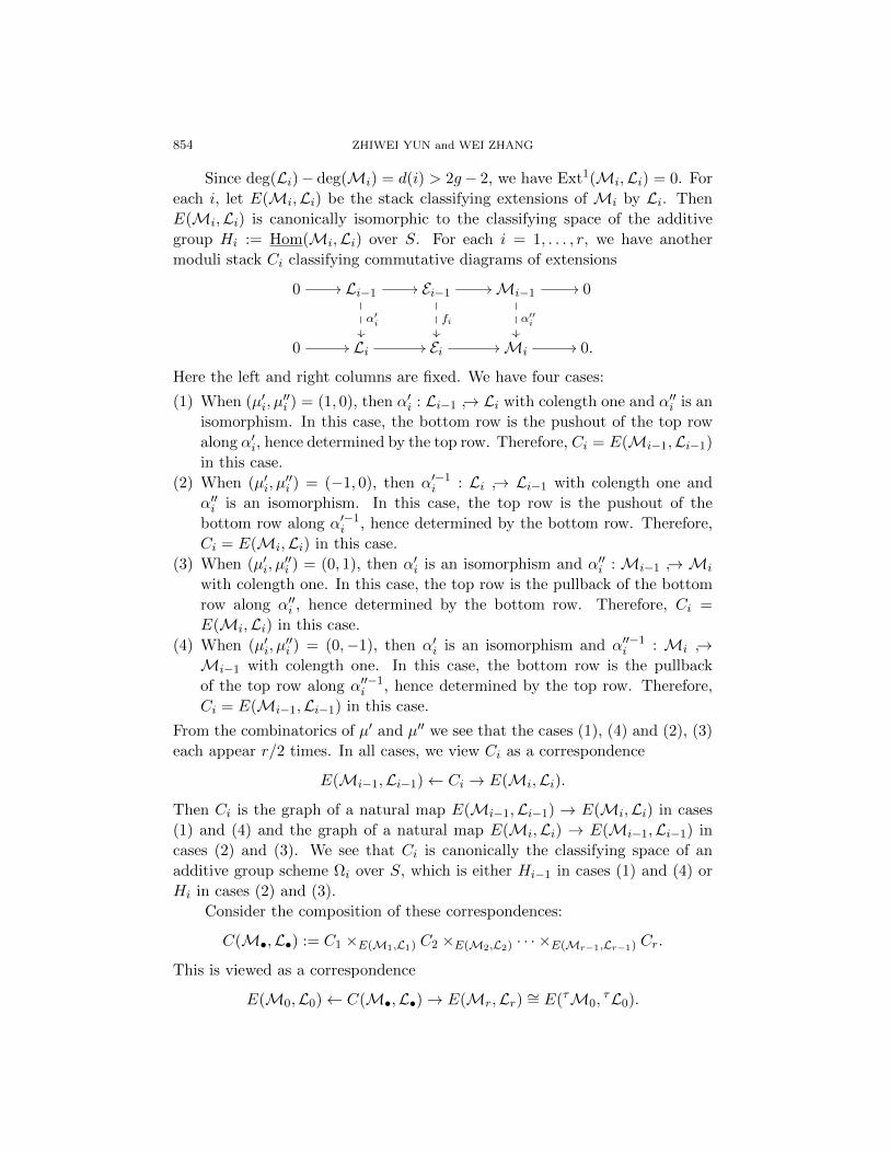
854 ZHIWEI YUN and WEI ZHANG
Since deg(Li)− deg(Mi) = d(i) > 2g− 2, we have Ext1(Mi,Li) = 0. For
each i, let E(Mi,Li) be the stack classifying extensions of Mi by Li. Then
E(Mi,Li) is canonically isomorphic to the classifying space of the additive
group Hi := Hom(Mi,Li) over S. For each i = 1, . . . , r, we have another
moduli stack Ci classifying commutative diagrams of extensions
0 // Li−1//
α′i
Ei−1//
fi
Mi−1//
α′′i
0
0 // Li // Ei //Mi// 0.
Here the left and right columns are fixed. We have four cases:
(1) When (µ′i, µ′′i ) = (1, 0), then α′i : Li−1 → Li with colength one and α′′i is an
isomorphism. In this case, the bottom row is the pushout of the top row
along α′i, hence determined by the top row. Therefore, Ci = E(Mi−1,Li−1)
in this case.
(2) When (µ′i, µ′′i ) = (−1, 0), then α′−1
i : Li → Li−1 with colength one and
α′′i is an isomorphism. In this case, the top row is the pushout of the
bottom row along α′−1i , hence determined by the bottom row. Therefore,
Ci = E(Mi,Li) in this case.
(3) When (µ′i, µ′′i ) = (0, 1), then α′i is an isomorphism and α′′i : Mi−1 → Mi
with colength one. In this case, the top row is the pullback of the bottom
row along α′′i , hence determined by the bottom row. Therefore, Ci =
E(Mi,Li) in this case.
(4) When (µ′i, µ′′i ) = (0,−1), then α′i is an isomorphism and α′′−1
i : Mi →Mi−1 with colength one. In this case, the bottom row is the pullback
of the top row along α′′−1i , hence determined by the top row. Therefore,
Ci = E(Mi−1,Li−1) in this case.
From the combinatorics of µ′ and µ′′ we see that the cases (1), (4) and (2), (3)
each appear r/2 times. In all cases, we view Ci as a correspondence
E(Mi−1,Li−1)← Ci → E(Mi,Li).
Then Ci is the graph of a natural map E(Mi−1,Li−1) → E(Mi,Li) in cases
(1) and (4) and the graph of a natural map E(Mi,Li) → E(Mi−1,Li−1) in
cases (2) and (3). We see that Ci is canonically the classifying space of an
additive group scheme Ωi over S, which is either Hi−1 in cases (1) and (4) or
Hi in cases (2) and (3).
Consider the composition of these correspondences:
C(M•,L•) := C1 ×E(M1,L1) C2 ×E(M2,L2) · · · ×E(Mr−1,Lr−1) Cr.
This is viewed as a correspondence
E(M0,L0)← C(M•,L•)→ E(Mr,Lr) ∼= E(τM0,τL0).

TAYLOR EXPANSION 855
To compute C(M•,L•) more explicitly, we consider the following situa-
tion. Let G be a group scheme over S with two subgroup schemes G1 and G2.
Then we have a canonical isomorphism of stacks over S
B(G1)×B(G) B(G2) ∼= G1\G/G2.
Using this fact repeatedly, and using that E(Mi,Li) = B(Hi) and Ci = B(Ωi),
we see that
(7.7) C(M•,L•) ∼= Ω1\H1
Ω2× H2
Ω3× · · ·
Ωr−1
× Hr−1/Ωr,
where Hi−1
Ωi× Hi means dividing by the diagonal action of Ωi on both Hi−1
and Hi by translations. Let
A(M•,L•) := H0
Ω1× H1
Ω2× · · ·
Ωr−1
× Hr−1
Ωr× Hr.
Since Ωi is always the smaller of Hi−1 and Hi, A(M•,L•) is an additive group
scheme over S. Then we have
(7.8) C(M•,L•) ∼= H0\A(M•,L•)/Hr.
Note that Hr∼= τH0 is the pullback of H0 via FrS . We have a relative
Frobenius map over S:
Fr/S : E(M0,L0) = B(H0)FrH0/S−−−−→ B(Hr) = E(Mr,Lr).
By the moduli meaning of ESht(M•,L•), we have a Cartesian diagram of stacks
ESht(M•,L•) //
C(M•,L•)
E(M0,L0)(id,Fr/S)
// E(M0,L0)× E(Mr,Lr).
Using the isomorphism (7.8), the above diagram becomes
ESht(M•,L•) //
H0\A(M•,L•)/Hr
B(H0)(id,FrH0/S
)// B(H)× B(Hr).
(7.9)
This implies that
(7.10) ESht(M•,L•) ∼= [A(M•,L•)/(id,FrH0/S)H0],
where H0 acts on A(M•,L•) via the embedding (id,FrH0/S) : H0 → H0 ×Hr
and the natural action of H0 × Hr on A(M•,L•). Since A is an additive
group scheme over S, hence smooth over S, the isomorphism (7.10) shows that
ESht(M•,L•) is smooth over S.

856 ZHIWEI YUN and WEI ZHANG
To compute the dimension of A(M•,L•), we compare dim Ωi with dimHi.
We have dimHi − dim Ωi = 1 in cases (1) and (4) and dimHi − dim Ωi = 0 in
cases (2) and (3). Since (1), (4) and (2), (3) each appear r/2 times, we have
dimA(M•,L•) = dimH0 +r∑i=1
(dimHi − dim Ωi) = dimH0 + r/2.
This implies ESht(M•,L•) is smooth of dimension r/2.
When S is a geometric point Spec(K), H0 and Hr can be viewed as
subspaces of the K-vector space A := A(M•,L•), and φ = FrH0/K : H0 →Hr is a morphism of group schemes over K. Choose a K-subspace L ⊂ A
complement to H0, then L ∼= Gr/2a as a group scheme over K. Consider the
homomorphism
α : H0 × L −→ A
given by (x, y) 7→ x + y + φ(x). By computing the tangent map of α at the
origin, we see that α is etale, therefore, Z = ker(α) is a finite etale group
scheme over K. We conclude that in this case the fiber of qd over S = Spec(K)
is
ESht(M•,L•) ∼= [A/(id,φ)H0] ∼= [L/Z] ∼= [Gr/2a /Z].
Corollary 7.6. Suppose d ∈ D satisfies d(i) > 2g − 2 for all i. Then
the cone of the map Rπ<dG,!Q` → Rπ≤dG,!Q` is isomorphic to πdH,!Q`[−r](−r/2),
which is a local system concentrated in degree r.
Proof. The cone of Rπ<dG,!Q` → Rπ≤dG,!Q` is isomorphic to RπdG,!Q`, where
πdG : ShtdG → Xr. By Lemma 7.4, for d ∈ D+, we have RπdG,!Q`∼= RπdB,!Q`.
By Lemma 7.5, qd is smooth of relative dimension r/2, and the relative funda-
mental cycles give Rqd,!Q` → Rrqd,!Q`[−r] → Q`[−r](−r/2), which is an iso-
morphism by checking the stalks (using the description of the geometric fibers
of qd given in Lemma 7.5). Therefore, RπdB,!Q`∼= RπdH,!Q`[−r](−r/2). Finally,
πdH : ShtdH → Xr is a Pic0X(k)-torsor by an argument similar to Lemma 5.13.
Therefore, RπdH,!Q` is a local system on Xr, and RπdG,!Q`∼= πdH,!Q`[−r](−r/2)
is a local system shifted to degree r.
7.3. Horocycles in the generic fiber. Fix a geometric generic point η of Xr.
For a stack X over Xr, we denote its fiber over η by Xη. Next we study the
cycles in ShtG,η given by images of ShtdB,η.
Lemma 7.7 (Drinfeld [5, Prop 4.2] for r = 2; Varshavsky [23, Prop 5.7]
in general). For each d ∈ D, the map pd,η : ShtdB,η → ShtG,η is finite and
unramified.
7.3.1. The cohomological constant term. Taking the geometric generic fiber
of the diagram (7.6), we view ShtdB,η as a correspondence between ShtG,η and

TAYLOR EXPANSION 857
ShtdH,η. The fundamental cycle of ShtdB,η (of dimension r/2) gives a cohomo-
logical correspondence between the constant sheaf on ShtG,η and the shifted
constant sheaf Q`[−r](−r/2) on ShtdH,η. Therefore, [ShtdB,η] induces a map
γd : Hrc(ShtG,η)(r/2)
p∗d,η−−→ Hr
c(ShtdB,η)(r/2)
[ShtdB,η
]−−−−−→ H0(ShtdB,η)
qd,η,!−−−→ H0(ShtdH,η).
(7.11)
Here we are implicitly using Lemma 7.7 to conclude that pd,η is proper, hence
p∗d,η induces a map between compactly supported cohomology groups.
Taking the product of γd for all d in a fixed Z-orbit δ ∈ D/Z, using the
decomposition (7.5), we get a map
(7.12) γδ : Hrc(ShtG,η)(r/2) −→
∏d∈δ
H0(ShtdH,η)∼= H0(Sht
µ(δ)1,η ).
When r = 0, (7.12) is exactly the constant term map for automorphic forms.
Therefore, we may call γδ the cohomological constant term map.
The right-hand side of (7.12) carries an action of the Hecke algebra HH =
⊗x∈|X|Q[tx, t−1x ]. In fact, Sht
µ(δ)1,η is a PicX(k)-torsor over Spec k(η). The action
of HH on Shtµ(δ)H,η is via the natural map HH
∼= Q[Div(X)]→ Q[PicX(k)].
Lemma 7.8. The map γδ in (7.12) intertwines the H -action on the left-
hand side and the HH-action on the right-hand side via the Satake transform
Sat : H →HH .
Proof. Since H is generated by hxx∈|X| as a Q-algebra, it suffices to
show that for any x ∈ |X|, the following diagram is commutative:
Hrc(ShtG,η)
C(hx)
γδ//∏d∈δ H0(ShtdH,η)
tx+qxt−1x
Hrc(ShtG,η)
γδ//∏d∈δ H0(ShtdH,η).
(7.13)
Let U = X − x. For a stack X over Xr, we use XUr to denote its
restriction to U r. Similar notation applies to morphisms over Xr.
Recall that ShtG,Ur(S) classifies (Ei;xi; fi; ι) such that xi are disjoint
from x. Hence the composition ι fr · · · f1 : E0 99K τE0 is an isomorphism
near x. In particular, the fiber E0,x = E0|S×x carries a Frobenius struc-
ture E0,x∼= τE0,x, hence E0,x descends to a two-dimensional vector space over
Spec kx (kx is the residue field of X at x) up to tensoring with a line. In other
words, there is a morphism ωx : ShtG,Ur → B(G(kx)) sending (xi; Ei; fi; ι) to
the descent of E0,x to Spec kx. In the following we shall understand that E0,x
is a two-dimensional vector space over kx, up to tensoring with a line over kx.
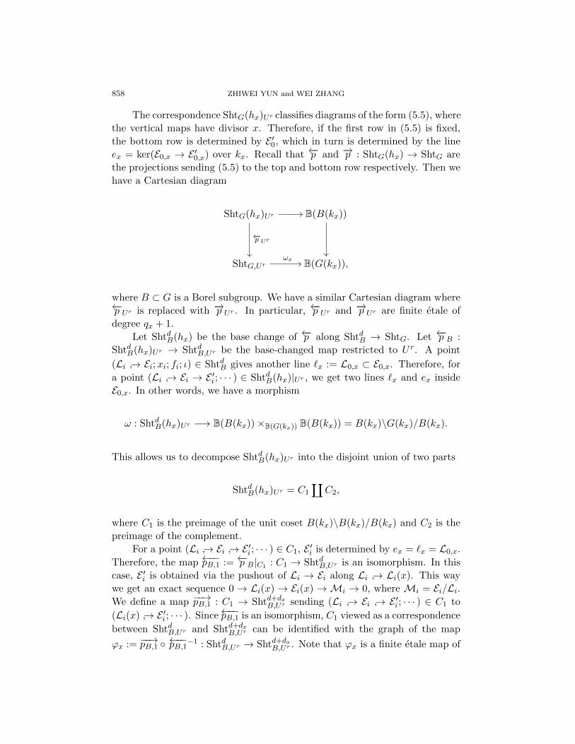
858 ZHIWEI YUN and WEI ZHANG
The correspondence ShtG(hx)Ur classifies diagrams of the form (5.5), where
the vertical maps have divisor x. Therefore, if the first row in (5.5) is fixed,
the bottom row is determined by E ′0, which in turn is determined by the line
ex = ker(E0,x → E ′0,x) over kx. Recall that ←−p and −→p : ShtG(hx) → ShtG are
the projections sending (5.5) to the top and bottom row respectively. Then we
have a Cartesian diagram
ShtG(hx)Ur //
←−p Ur
B(B(kx))
ShtG,Urωx// B(G(kx)),
where B ⊂ G is a Borel subgroup. We have a similar Cartesian diagram where←−p Ur is replaced with −→p Ur . In particular, ←−p Ur and −→p Ur are finite etale of
degree qx + 1.
Let ShtdB(hx) be the base change of ←−p along ShtdB → ShtG. Let ←−p B :
ShtdB(hx)Ur → ShtdB,Ur be the base-changed map restricted to U r. A point
(Li → Ei;xi; fi; ι) ∈ ShtdB gives another line `x := L0,x ⊂ E0,x. Therefore, for
a point (Li → Ei → E ′i; · · · ) ∈ ShtdB(hx)|Ur , we get two lines `x and ex inside
E0,x. In other words, we have a morphism
ω : ShtdB(hx)Ur −→ B(B(kx))×B(G(kx)) B(B(kx)) = B(kx)\G(kx)/B(kx).
This allows us to decompose ShtdB(hx)Ur into the disjoint union of two parts
ShtdB(hx)Ur = C1
∐C2,
where C1 is the preimage of the unit coset B(kx)\B(kx)/B(kx) and C2 is the
preimage of the complement.
For a point (Li → Ei → E ′i; · · · ) ∈ C1, E ′i is determined by ex = `x = L0,x.
Therefore, the map ←−−pB,1 :=←−p B|C1 : C1 → ShtdB,Ur is an isomorphism. In this
case, E ′i is obtained via the pushout of Li → Ei along Li → Li(x). This way
we get an exact sequence 0 → Li(x) → Ei(x) →Mi → 0, where Mi = Ei/Li.We define a map −−→pB,1 : C1 → Shtd+dx
B,Ur sending (Li → Ei → E ′i; · · · ) ∈ C1 to
(Li(x) → E ′i; · · · ). Since←−−pB,1 is an isomorphism, C1 viewed as a correspondence
between ShtdB,Ur and Shtd+dxB,Ur can be identified with the graph of the map
ϕx := −−→pB,1 ←−−pB,1−1 : ShtdB,Ur → Shtd+dxB,Ur . Note that ϕx is a finite etale map of

TAYLOR EXPANSION 859
degree qx. We have a commutative diagram
ShtdH,Ur Γ(tx)id
ootx
// Shtd+dxH,Ur
ShtdB,Ur
pd
qd
OO
C1 = Γ(ϕx)
OO
←−−pB,1
∼oo
−−→pB,1// Shtd+dx
B,Ur
pd+dx
qd+dx
OO
ShtG,Ur ShtG(hx)Ur←−p
oo
−→p// ShtG,Ur .
Here Γ(tx) is the graph of the isomorphism ShtdH,Ur → Shtd+dxH,Ur given by tensor-
ing the line bundles with O(x). Therefore, the action of [C1] on the compactly
supported cohomology of the generic fiber of ShtdB fits into a commutative
diagram
Hrc(ShtdB,η)(r/2)
[C1]
[ShtdB,η
]// H0(ShtdB,η)
ϕx,∗
// H0(ShtdH,η)
tx
Hrc(Shtd+dx
B,η )(r/2)[Shtd+dx
B,η]// H0(Shtd+dx
B,η ) // H0(Shtd+dxH,η ).
(7.14)
Similarly, for C2, we define a morphism −−→pB,2 : C2 → Shtd−dxB,Ur sending
(Li → Ei → E ′i; · · · ) ∈ C2 to (Li → E ′i; · · · ). Then −−→pB,2 is an isomorphism
while ←−p B,2 = ←−p B|C2 is finite etale of degree qx. Therefore, C2 viewed as a
correspondence between ShtdB,Ur and Shtd−dxB,Ur can be identified with the trans-
pose of the graph of the map ϕx : Shtd−dxB,Ur → ShtdB,Ur defined previously. We
also have a commutative diagram
ShtdH,Ur Γ(t−1x )
idoo
t−1x
// Shtd−dxH,Ur
ShtdB,Ur
pd
qd
OO
C2 = tΓ(ϕx)
OO
←−−pB,2oo
−−→pB,2∼
// Shtd−dxB,Ur
pd−dx
qd−dx
OO
ShtG,Ur ShtG(hx)Ur←−p
oo
−→p// ShtG,Ur .

860 ZHIWEI YUN and WEI ZHANG
The action of [C2] on the compactly supported cohomology of the generic fibers
of ShtdB fits into a commutative diagram
Hrc(ShtdB,η)(r/2)
[C2]=ϕ∗x
[ShtdB,η
]// H0(ShtdB,η) // H0(ShtdH,η).
Hrc(Shtd−dxB,η )(r/2)
[Shtd−dxB,η
]// H0(Shtd−dxB,η ) //
q−1x ϕx,∗
OO
H0(Shtd−dxH,η )
q−1x tx
OO
(7.15)
The appearance of qx in the above diagram is because the degree of ϕx is qx.
Combining (7.14) and (7.15) we get a commutative diagram∏d∈δ Hr
c(ShtdB,η)(r/2) //
[C1]+[C2]
∏d∈δ H0(ShtdH,η)
tx+qxt−1x
∏d∈δ Hr
c(ShtdB,η)(r/2) //∏d∈δ H0(ShtdH,η).
(7.16)
Finally, let −→pB : ShtdB(hx)Ur → ShtdB,Ur be −−→pB,1 on C1 and −−→pB,2 on C2.
Consider the commutative diagram
∐d∈δ ShtdB(hx)Ur
(pd)d∈δ
−→pB//∐d∈δ ShtdB,Ur
(pd)d∈δ
ShtG(hx)Ur−→p
// ShtG,Ur .
Since −→pB and −→p are both finite etale of degree qx + 1, by examining geometric
fibers we conclude that the above diagram is Cartesian. The similar diagram
with −→pB and −→p replaced with←−pB and←−p is Cartesian by definition. From these
facts we get a commutative diagram
Hrc(ShtG,η)
C(hx)
(p∗d)d∈δ//∏d∈δ Hr
c(ShtdB,η)
[C1]+[C2]
Hrc(ShtG,η)
(p∗d)d∈δ//∏d∈δ Hr
c(ShtdB,η).
Combining this with (7.16) we obtain (7.13), as desired.
7.4. Finiteness. For fixed d ∈ D, the Leray spectral sequence associ-
ated with the map π≤dG gives an increasing filtration L≤iH2rc (Sht≤dG ⊗k k) on
H2rc (Sht≤dG ⊗k k), with L≤iH
2rc (Sht≤dG ⊗k k) being the image of
H2r(Xr ⊗k k, τ≤iRπ≤dG,!Q`) −→ H2r(Xr ⊗k k,Rπ≤dG,!Q`) ∼= H2rc (Sht≤dG ⊗k k).
Here τ≤i means the truncation in the usual t-structure ofDbc(X
r,Q`). Let L≤iV
be the inductive limit lim−→d∈D L≤iH2rc (Sht≤dG ⊗k k)(r), which is a subspace of V .

TAYLOR EXPANSION 861
This way we get a filtration on V :
0 ⊂ L≤0V ⊂ L≤1V ⊂ · · · ⊂ L≤2rV = V.
Lemma 7.9. Each L≤iV is stable under the action of H .
Proof. The map C(hD)d,d′ in (7.1) induces τ≤iC(hD)d,d′ : τ≤iRπ≤dG,!Q` →
τ≤iRπ≤d′G,! Q`. By the construction of C(hD) we have a commutative diagram
lim−→dH2r(Xr ⊗k k, τ≤iRπ≤dG,!Q`)
lim−→ τ≤iC(hD)d,d′//
lim−→d′H2r(Xr ⊗k k, τ≤iRπ≤d
′
G,! Q`)
H2rc (ShtG ⊗k k)
C(hD)// H2r
c (ShtG ⊗k k).
The image of the vertical maps are both L≤iV up to a Tate twist; therefore,
L≤iV is stable under C(hD). When D runs over all effective divisors on X,
C(hD) span H , hence L≤iV is stable under H .
Lemma 7.10. For i 6= r, GrLi V := L≤iV/L≤i−1V is finite dimensional
over Q`.
Proof. We say d ∈ D is large if d(i) > 2g − 2 for all i. In the following
argument it is convenient to choose a total order on D that extends its partial
order. Under the total order, Sht<dG =∐d′<d Shtd
′G and Sht≤dG =
∐d′≤d ShtdG are
different from their original meanings, and we will use the new notion during
the proof.
By Corollary 7.6, the inductive system τ≤r−1Rπ≤dG,!Q` stabilizes for d large.
Hence so does L≤r−1H2rc (Sht≤dG ⊗k k). Therefore, L≤r−1V is finite dimensional.
It remains to show that V/L≤rV is finite dimensional. Again by Corol-
lary 7.6, for d large, the map Rr+1π<dG,!Q` → Rr+1π≤dG,!Q` is surjective because
the next term in the long exact sequence is Rr+1πdG,!Q` = 0. This implies
that the inductive system Rr+1π≤dG,!Q` is eventually stable because any chain
of surjections F1 F2 · · · of constructible sheaves on Xr has to stabilize;
i.e., constructible Q`-sheaves satisfy the ascending chain condition. Also by
Corollary 7.6, the inductive system τ>r+1Rπ≤dG,!Q` is stable. Combined with
the stability of Rr+1π≤dG,!Q`, we see that the system τ>rRπ≤dG,!Q` is stable. In
other words, there exists a large d0 ∈ D such that for any d ≥ d0, the natural
map τ>rRπ<dG,!Q` → τ>rRπ
≤dG,!Q` is an isomorphism.
We abbreviate H2rc (Sht<dG ⊗k k) by H<d and H2r
c (Sht≤dG ⊗k k) by H≤d. For
d ≥ d0, the distinguished triangle of functors τ≤r → id → τ>r → applied to

862 ZHIWEI YUN and WEI ZHANG
Rπ<dG,!Q` and Rπ≤dG,!Q` gives a morphism of exact sequences
L≤rH<d//
H<d//
H2r(Xr ⊗k k, τ>rRπ<dG,!Q`) //
o
· · ·
L≤rH≤d // H≤d // H2r(Xr ⊗k k, τ>rRπ≤dG,!Q`) // · · · .
Therefore, the inductive system H≤d/L≤rH≤d is a subsystem of
H2r(Xr ⊗k k, τ>rRπ≤dG,!Q`),
which is stable with finite-dimensional inductive limit. Hence the inductive sys-
tem H≤d/L≤rH≤d is itself stable with finite-dimensional inductive limit. Tak-
ing inductive limit, using that V = lim−→dH≤d(r) and L≤iV = lim−→d
L≤iH≤d(r),
we see that V/L≤rV ∼= lim−→dH≤d(r)/L≤rH≤d(r) is finite dimensional.
Lemma 7.11. The space IEis · (L≤rV ) is finite dimensional over Q`.
Proof. Let U ⊂ ShtG be the union of those Sht≤dG for d ∈ D such that
mini∈Z/rZd(i) ≤ 2g − 2. Since inst(E) has an absolute lower bound, there
are only finitely many such d with ShtdG 6= ∅, hence U is an open substack of
finite type. Let πUG : U → Xr be the restriction of πG. For f ∈ H , and any
d ∈ D, its action defines a map C(f)d,d′ : Riπ≤dG,!Q` → Riπ≤d′
G,! Q` for sufficiently
large d′. We may assume d′ > 2g − 2 , which means d′(j) > 2g − 2 for all j.
We shall show that when f ∈ IEis and i ≤ r, the image of C(f)d,d′ is contained
in the image of the map ιU,d′ : RiπUG,!Q` → Riπ≤d′
G,! Q` induced by the inclusion
U ⊂ Sht≤d′
G , which implies the proposition. In other words, we need to show
that the composition ϕ : Riπ≤dG,!Q`
C(f)d,d′−−−−−→ Riπ≤d′
G,! Q` → coker(ιU,d′) is zero.
By Corollary 7.6, either ιU,d′ is an isomorphism (if i < r) or when i = r,
coker(ιU,d′) is a subsheaf of a local system on Xr. Therefore, to show that ϕ
is zero, it suffices to show that ϕ vanishes at the generic point of Xr.
Let η be a geometric generic point of Xr. We use a subscript η to denote
the fibers over η, as in Section 7.3. Let ιU : Hrc(Uη) → Hr
c(ShtG,η) be the
map induced by the inclusion of U . It suffices to show that for f ∈ IEis, the
composition Hrc(ShtG,η)
f∗−→ Hrc(ShtG,η) Hr
c(ShtG,η)/ιU (Hrc(Uη)) is zero.
Recall from (7.11) the cohomological constant term map γd : Hrc(ShtG,η)→
H0(ShtdH,η). By the definition of γd, for d > 2g−2, γd factors through the quo-
tient Hrc(ShtG,η)/ιU (Hr
c(Uη)) and induces a map
γ+ :=∏
d>2g−2
γd : Hrc(ShtG,η)/ιU (Hr
c(Uη)) −→∏
d>2g−2
H0(ShtdH,η).
Both sides of the above map admit filtrations indexed by the poset d ∈ D; d >
2g − 2: on the left-hand side this is given by the image of Hrc(Sht≤dG,η), and
TAYLOR EXPANSION 863
on the right-hand side this is given by∏
2g−2<d′≤d H0(Shtd′H,η). The map γ+
respects these filtrations, and by Corollary 7.6, the associated graded map of
γ+ under these filtrations is injective. Therefore, γ+ is injective.By Lemma 7.8, we have a commutative diagram
Hrc(ShtG,η)(r/2)
f∗//∏
γd
Hrc(ShtG,η)(r/2) //∏
γd
Hrc(ShtG,η)(r/2)/ιU (Hr
c(Uη))(r/2)
γ+
∏d∈D H0(ShtdH,η)
Sat(f)∗//∏d∈D H0(ShtdH,η) //
∏d>2g−2 H0(ShtdH,η).
Since the action of HH on∏d∈D H0(ShtdH,η) factors through Q`[PicX(k)],
Sat(f) acts by zero in the bottom arrow above. Since γ+ is injective, the
composition of the top row is also zero, as desired.
Definition 7.12. We define the Q`-algebra H` to be the image of the map
H ⊗Q` −→ EndQ`(V )×Q`[PicX(k)]ιPic ,
the product of the action map on V and aEis ⊗Q`.
Lemma 7.13.
(1) For any x ∈ |X|, V is a finitely generated Hx ⊗Q`-module.
(2) The Q`-algebra H` is finitely generated over Q` and is a ring with Krull
dimension one.
Proof. (1) Let D≤n ⊂ D be the subset of those d such that minid(i) ≤2g− 2 +ndx. Let Dn = D≤n−D≤n−1. For each n ≥ 0, let Un = ∪d∈D≤nSht≤dG .
Then U0 ⊂ U1 ⊂ · · · are finite type open substacks of ShtG that exhaust ShtG.
Let πn : Un → Xr be the restriction of πG, and let Kn = Rπn,!Q`. The
inclusion Un → Un+1 induces maps ιn : Kn → Kn+1. Let Cn+1 be the cone of
ιn. Then by Corollary 7.6, when n ≥ 0, Cn+1 is a successive extension of shifted
local systems πdH,!Q`[−r](−r/2) for those d ∈ Dn+1. In particular, for n ≥ 0,
Cn+1 is a shifted local system in degree r and pure of weight 0 as a complex.
By construction, the action of hx ∈Hx on H∗c(ShtG ⊗k k) is induced from
the correspondence ShtG(hx), which restricts to a correspondence ≤nShtG(hx)
=←−p −1(Un) between Un and Un+1. Similar to the construction of C(hx)d,d′ in
(7.1), the fundamental class of ≤nShtG(hx) gives a map C(hx)n : Kn → Kn+1.
Since C(hx)nιn−1 = ιnC(hx)n−1, we have the induced map τn : Cn → Cn+1.
We claim that τn is an isomorphism for n > 0. In fact, since Cn and Cn+1 are
local systems in degree r, it suffices to check that τn induces an isomorphism
between the geometric generic stalks Cn,η and Cn+1,η. By Corollary 7.6, we
have an isomorphism induced from the maps γd for d ∈ Dn (cf. (7.11)):
Cn,η ∼=⊕d∈Dn
H0(ShtdH,η).

864 ZHIWEI YUN and WEI ZHANG
By Lemma 7.8, τn,η : Cn,η → Cn+1,η is the same as the direct sum of the isomor-
phisms tx : H0(ShtdH,η)→ H0(Shtd+dxH,η ). (The other term qxt
−1x : H0(ShtdH,η)→
H0(Shtd−dxH,η ) does not appear because d−dx ∈ D≤n−1, hence the corresponding
contribution becomes zero in Cn+1,η.) Therefore, τn,η is an isomorphism, hence
so is τn.
We claim that there exists n0 ≥ 0 such that for any n ≥ n0, the map
W≤2rH2r+1(Xr ⊗k k,Kn) −→W≤2rH
2r+1(Xr ⊗k k,Kn+1)
is an isomorphism. Here W≤2r is the weight filtration using Frobenius weights.
In fact, the next term in the long exact sequence is W≤2rH2r+1(Xr ⊗k k,Cn+1),
which is zero because Cn+1 is pure of weight 0. Therefore, the natural map
W≤2rH2r+1(Xr ⊗k k,Kn) → W≤2rH
2r+1(Xr ⊗k k,Kn+1) is always surjective
for n ≥ 0, hence it has to be an isomorphism for sufficiently large n.
The triangle Kn → Kn+1 → Cn+1 → Kn[1] gives a long exact sequence
H2r(Xr ⊗k k,Kn) −→ H2r(Xr ⊗k k,Kn+1) −→ H2r(Xr ⊗k k,Cn+1)(7.17)
−→W≤2rH2r+1(Xr ⊗k k,Kn) −→W≤2rH
2r+1(Xr ⊗k k,Kn+1).
Here we are using the fact that H2r(Xr ⊗k k,Cn+1) is pure of weight 2r (since
Cn+1 is pure of weight 0). For n ≥ n0, the last map above is an isomorphism;
therefore, the first row of (7.17) is exact on the right.
Let F≤nV be the image of
H2r(Xr ⊗k k,Kn)(r) −→ lim−→n
H2r(Xr ⊗k k,Kn)(r) = V.
Then for n ≥ n0, the exactness of (7.17) implies H2r(Xr ⊗k k,Cn+1)(r) GrFn+1V for n ≥ n0. The Hecke operator C(hx) sends F≤nV to F≤n+1V and
induces a map GrFnC(hx) : GrFnV → GrFn+1V . We have a commutative diagram
for n ≥ n0:
H2r(Xr ⊗k k,Cn)(r)
H2r(Xr⊗kk,τn)// H2r(Xr ⊗k k,Cn+1)(r)
GrFnVGrFnC(hx)
// GrFn+1V.
The fact that τn : Cn → Cn+1 is an isomorphism implies that GrFnC(hx) is
surjective for n ≥ n0. Therefore, the action map
Hx ⊗Q F≤n0V = Q[hx]⊗Q F≤n0V −→ V
is surjective by checking the surjectivity on the associated graded. Since F≤n0V
is finite dimensional over Q`, V is finitely generated as an Hx ⊗Q`-module.
(2) We have H` ⊂ EndHx⊗Q`(V ⊕ Q`[PicX(k)]ιPic). Since both V and
Q`[PicX(k)]ιPic are finitely generated Hx⊗Q`-modules by Part (1) and Lemma

TAYLOR EXPANSION 865
4.2, EndHx⊗Q`(V ⊕ Q`[PicX(k)]ιPic) is also finitely generated as an Hx ⊗ Q`-
module. Since Hx ⊗ Q` is a polynomial ring in one variable over Q`, H`
is a finitely generated algebra over Q` of Krull dimension at most one. Since
H` → Q`[PicX(k)]ιPic is surjective by Lemma 4.2 and Q`[PicX(k)]ιPic has Krull
dimension one, H` also has Krull dimension one.
The map aEis : H` → Q`[PicX(k)]ιPic is surjective by Lemma 4.2(2). It
induces a closed embedding Spec(aEis) : ZEis,Q` = SpecQ`[PicX(k)]ιPic →Spec H`.
Theorem 7.14 (Cohomological spectral decomposition).
(1) There is a decomposition of the reduced scheme of Spec H` into a disjoint
union
(7.18) SpecÄH`
äred= ZEis,Q`
∐Zr0,`,
where Zr0,` consists of a finite set of closed points. There is a unique de-
compositionV = VEis ⊕ V0
into H ⊗Q`-submodules, such that Supp(VEis) ⊂ ZEis,Q` and Supp(V0) =
Zr0,`.4
(2) The subspace V0 is finite dimensional over Q`.
Proof. (1) Let V ′ = L≤rV . Let IEis ⊂ H` be the ideal generated by
the image of IEis. By Lemma 7.13, V ′ is a submodule of a finitely generated
module V over the noetherian ring H`; therefore, V ′ is also finitely generated.
By Lemma 7.11, IEisV′ is a finite-dimensional H`-submodule of V ′. Let Z ′ ⊂
Spec(H`)red be the finite set of closed points corresponding to the action of H`
on IEisV′. We claim that Supp(V ′) is contained in the union ZEis,Q` ∪ Z ′. In
fact, suppose f ∈H` lies in the defining radical ideal J of ZEis,Q` ∪ Z ′. Then
after replacing f by a power of it, we have f ∈ IEis (since J is contained in
the radical of IEis), and f acts on IEisV′ by zero. Therefore, f2 acts on V ′ by
zero, hence f lies in the radical ideal defining Supp(V ′).
By Lemma 7.10, V/V ′ is finite dimensional. Let Z ′′ ⊂ Spec(H`)red be the
support of V/V ′ as a H`-module, which is a finite set. Then Spec(H`)red =
Supp(V ) ∪ ZEis,Q` = ZEis,Q` ∪ Z ′ ∪ Z ′′. Let Zr0,` = (Z ′ ∪ Z ′′) − ZEis,Q` ; we get
the desired decomposition (7.18).
According to (7.18), the finitely generated H`-module V , viewed as a
coherent sheaf on Spec H`, can be uniquely decomposed into
V = VEis ⊕ V0
with Supp(VEis) ⊂ ZEis,Q` and Supp(V0) = Zr0,`.
4When we talk about the support of a coherent module M over a Noetherian ring R, we
always mean a closed subset of SpecR with the reduced scheme structure.

866 ZHIWEI YUN and WEI ZHANG
(2) We know that V0 is a coherent sheaf on the scheme Spec H` that is of
finite type over Q`, and we know that Supp(V0) = Zr0,` is finite. Therefore, V0
is finite dimensional over Q`.
7.4.1. The case r = 0. Let us reformulate the result in Theorem 7.14 in
the case r = 0 in terms of automorphic forms. Let A = Cc(G(F )\G(AF )/K,Q)
be the space of compactly supported Q-valued unramified automorphic forms,
where K =∏xG(Ox). This is a Q-form of the Q`-vector space V for r = 0.
Let Haut be the image of the action map H → EndQ(A)×Q[PicX(k)]ιPic . The
Q`-algebra Haut,Q` := Haut ⊗ Q` is the algebra H` defined in Definition 7.12
for r = 0.
Theorem 7.14 for r = 0 reads
(7.19) Spec H redaut,Q` = ZEis,Q`
∐Z0
0,`,
where Z00,` is a finite set of closed points. Below we will strengthen this de-
composition to work over Q and link Z00,` to the set of cuspidal automorphic
representations.
7.4.2. Positivity and reducedness. The first thing to observe is that Haut
is already reduced. In fact, we may extend the Petersson inner product on Ato a positive definitive quadratic form on AR. By the r = 0 case of Lemma 7.2,
Haut acts on AR as self-adjoint operators. Its image in End(A) is therefore
reduced. Since Q[PicX(k)]ιPic is reduced as well, we conclude that Haut is
reduced.
Let Acusp ⊂ A be the finite-dimensional Q-vector space of cusp forms.
Let Hcusp be the image of Haut in EndQ(Acusp). Then Hcusp is a reduced
artinian Q-algebra, hence a product of fields. Let Zcusp = Spec Hcusp. Then a
point in Zcusp is the same as an everywhere unramified cuspidal automorphic
representation π ofG in the sense of Section 1.2. Therefore, we have a canonical
isomorphism
Hcusp =∏
π∈Zcusp
Eπ,
where Eπ is the coefficient field of π.
Lemma 7.15.
(1) There is a canonical isomorphism of Q-algebras
Haut∼= Q[PicX(k)]ιPic ×Hcusp.
Equivalently, we have a decomposition into disjoint reduced closed sub-
schemes
(7.20) Spec Haut = ZEis
∐Zcusp.
(2) We have Z00,` = Zcusp,Q` , the base change of Zcusp from Q to Q`.

TAYLOR EXPANSION 867
Proof. (1) The Q version of Lemma 7.13 says that Haut is a finitely gen-
erated Q-algebra and that A is a finitely generated Haut-module. By the same
argument of Theorem 7.14, we get a decomposition
(7.21) Spec H redaut = Spec Haut = ZEis
∐Z0,
where Z0 is a finite collection of closed points. Correspondingly we have a
decomposition
A = AEis ⊕A0
with Supp(AEis) ⊂ ZEis and Supp(A0) = Z0. Since A0 is finitely generated
over Haut with finite support, it is finite dimensional over Q. Since A0 is finite
dimensional and stable under H , we necessarily have A0 ⊂ Acusp. (See [15,
Lemme 8.13]; in fact in our case it can be easily deduced from the r = 0 case
of Lemma 7.8.)
We claim that A0 = Acusp. To show the inclusion in the other direction, it
suffices to show that any cuspidal Hecke eigenform ϕ ∈ Acusp⊗Q lies in A0⊗Q.
Suppose this is not the case for ϕ, letting λ : H → Q be the character by which
H acts on ϕ; then λ /∈ Z0(Q). By (7.21), λ ∈ ZEis(Q), which means that the
action of H on ϕ factors through Q[PicX(k)] via aEis, which is impossible.
Now A0 = Acusp implies that Z0 = Supp(A0) = Supp(Acusp) = Zcusp.
Combining with (7.21), we get (7.20).
Part (2) follows from comparing (7.19) to the base change of (7.20) to Q`.
7.5. Decomposition of the Heegner–Drinfeld cycle class. In previous sub-
sections, we have been working with the middle-dimensional cohomology (with
compact support) of ShtG = ShtrG, and we established a decomposition of it
as an HQ`-module. Exactly the same argument works if we replace ShtG with
Sht′G = Sht′rG. Instead of repeating the argument we simply state the corre-
sponding result for Sht′G in what follows.
Let
V ′ = H2rc (Sht′G ⊗k k,Q`)(r).
Then V ′ is equipped with a Q`-valued cup product pairing
(7.22) (·, ·) : V ′ ⊗Q` V′ −→ Q`
and an action of H by self-adjoint operators.
Similar to Definition 7.12, we define the Q`-algebra H`′
to be the image
of the map
H ⊗Q` −→ EndQ`(V′)×Q`[PicX(k)]ιPic .
Theorem 7.16 (Variant of Lemma 7.13 and Theorem 7.14).
(1) For any x ∈ |X|, V ′ is a finitely generated Hx ⊗Q`-module.

868 ZHIWEI YUN and WEI ZHANG
(2) The Q`-algebra H`′
is finitely generated over Q` and is one dimensional
as a ring.
(3) There is a decomposition of the reduced scheme of Spec H`′
into a disjoint
union
(7.23) SpecÄH`′äred
= ZEis,Q`∐
Z ′r0,`,
where Z ′r0,` consists of a finite set of closed points. There is a unique de-
composition
V ′ = V ′Eis ⊕ V ′0into H ⊗Q`-submodules, such that Supp(V ′Eis) ⊂ ZEis,Q` and Supp(V ′0) =
Z ′r0,`.
(4) The subspace V ′0 is finite dimensional over Q`.
We may further decompose V ′Q`:= V ′ ⊗Q` Q` according to points in
Z ′r0,`(Q`). A point in Z ′r0,`(Q`) is a maximal ideal m ⊂ HQ`, or equivalently
a ring homomorphism H → Q` whose kernel is m. We have a decomposition
(7.24) V ′Q`= V ′
Eis,Q`⊕( ⊕m∈Z′r
0,`(Q`)
V ′m
).
Then V ′m is characterized as the largest Q`-subspace of V ′Q`on which the action
of m is locally nilpotent. By Theorem 7.16, V ′m turns out to be the localization
of V ′ at the maximal ideal m, hence our notation V ′m is consistent with the
standard notation used in commutative algebra.
We may decompose the cycle class cl(θµ∗ [ShtµT ]) ∈ V ′Q`according to the
decomposition (7.24),
(7.25) cl(θµ∗ [ShtµT ]) = [ShtT ]Eis +∑
m∈Zr0,`
(Q`)
[ShtT ]m,
where [ShtT ]Eis ∈ V ′Eis and [ShtT ]m ∈ V ′m.
Corollary 7.17.
(1) The decomposition (7.24) is an orthogonal decomposition under the cup
product pairing (7.22) on V ′.
(2) For any f ∈H , we have
(7.26) Ir(f) = ([ShtT ]Eis, f ∗ [ShtT ]Eis) +∑
m∈Z′r0,`
(Q`)
Ir(m, f),
where
Ir(m, f) := ([ShtT ]m, f ∗ [ShtT ]m) .

TAYLOR EXPANSION 869
Proof. The orthogonality of the decomposition (7.24) follows from the
self-adjointness of H with respect to the cup product pairing, i.e., variant of
Lemma 7.2 for Sht′G. The formula (7.26) then follows from the orthogonality
of the terms in the decomposition (7.25).
Part 3. The comparison
8. Comparison for most Hecke functions
The goal of this section is to prove the key identity (1.9) for most Hecke
functions. More precisely, we will prove the following theorem.
Theorem 8.1. Let D be an effective divisor on X of degree d ≥ max2g′−1, 2g. Then for any u ∈ P1(F )− 1, we have
(8.1) (log q)−rJr(u, hD) = Ir(u, hD).
In particular, we have
(8.2) (log q)−rJr(hD) = Ir(hD).
For the definition of Jr(u, hD) and Ir(u, hD), see (2.16) and (6.11) respec-
tively.
8.1. Direct image of fM.
8.1.1. The local system L(ρi). Let j : Xd ⊂ Xd ⊂ “Xd be the locus of
multiplicity-free divisors. Taking the preimage of Xd under the branched cover
X ′d → Xd → Xd, we get an etale Galois cover
u : X ′d, −→ Xd, −→ Xd
with Galois group Γd := ±1d o Sd. For 0 ≤ i ≤ d, let χi be the character
±1d → ±1 that is nontrivial on the first i factors and trivial on the
rest. Let Si,d−i ∼= Si × Sd−i be the subgroup of Sd stabilizing 1, 2, . . . , i ⊂1, . . . , d. Then χi extends to the subgroup Γd(i) = ±1doSi,d−i of Γd with
the trivial representation on the Si,d−i-factor. The induced representation
(8.3) ρi = IndΓdΓd(i)(χi 1)
is an irreducible representation of Γd. This representation gives rise to an irre-
ducible local system L(ρi) on Xd . Let Ki := j!∗(L(ρi)[d])[−d] be the middle ex-
tension of L(ρi); see [3, 2.1.7]. Then Ki is a shifted simple perverse sheaf on “Xd.
Proposition 8.2. Suppose d ≥ 2g′ − 1. Then we have a canonical iso-
morphism of shifted perverse sheaves
(8.4) RfM,∗Q`∼=
d⊕i,j=0
(Ki Kj)|Ad .
Here KiKj lives on “Xd×PicdX“Xd, which contains Ad as an open subscheme.
870 ZHIWEI YUN and WEI ZHANG
Proof. By Proposition 6.1(4), fM is the restriction of νd × νd : “X ′d ×PicdX“X ′d → “Xd ×PicdX“Xd, where νd : “X ′d → “Xd is the norm map. By Proposi-
tion 6.1(3), νd is also proper. Therefore, by the Kunneth formula, it suffices
to show that
(8.5) Rνd,∗Q`∼=
d⊕i=0
Ki.
We claim that νd is a small map (see [10, 6.2]). In fact the only positive
dimension fibers are over the zero section PicdX → “Xd, which has codimension
d − g + 1. On the other hand, the restriction of νd to the zero section is
the norm map PicdX′ → PicdX , which has fiber dimension g − 1. The condition
d ≥ 2g′−1 ≥ 3g−2 implies d−g+1 ≥ 2(g−1)+1; therefore, νd is a small map.
Now νd is proper, small with smooth and geometrically irreducible source,
and Rνd,∗Q` is the middle extension of its restriction to any dense open subset
of “Xd (see [10, Th. at the end of 6.2]). In particular, Rνd,∗Q` is the middle
extension of its restriction to Xd . It remains to show
(8.6) Rνd,∗Q`|Xd
∼=d⊕i=0
L(ρi).
Let νd : X ′d = ν−1d (Xd) → Xd be the restriction of νd : X ′d → Xd
over Xd . Then Rνd,∗Q` is the local system on Xd associated with the rep-
resentation IndΓdSdQ` = Q`[Γd/Sd] of Γd. A basis 1ε of Q`[Γd/Sd] is given
by the indicator functions of the Sd-coset of ε ∈ ±1d. For any character
χ : ±1d → ±1, let 1χ :=∑ε χ(ε)1ε ∈ Q`[Γd/Sd]. For the character χi
considered in Section 8.1.1, 1χi is invariant under Si,d−i, and therefore, we have
a Γd-equivariant embedding ρi = IndΓdΓd(i)(χi1) → Q`[Γd/Sd]. Checking total
dimensions we conclude that
Q`[Γd/Sd] ∼=d⊕i=0
ρi.
This gives a canonical isomorphism of local systems Rνd,∗Q`∼= ⊕di=0L(ρi),
which is (8.6).
In Section 6.2.3, we have defined a self-correspondence H = Hk1M,d ofMd
overAd. Recall thatA♦d ⊂ Ad is the open subscheme “Xd×PicdXXd, andM♦d and
H♦ are the restrictions ofMd and H to A♦d . Recall that [H♦] ∈ Ch2d−g+1(H)Qis the fundamental cycle of the closure of H♦.
Proposition 8.3. Suppose d ≥ 2g′ − 1. Then the action fM,![H♦] on
RfM∗Q` preserves each direct summand Ki Kj under the decomposition
(8.4) and acts on Ki Kj by the scalar (d− 2j).

TAYLOR EXPANSION 871
Proof. By Proposition 8.2, RfM∗Q` is a shifted perverse sheaf all of whose
simple constituents have full support. Therefore, it suffices to prove the same
statement after restricting to any dense open subset U ⊂ Ad. We work with
U = A♦d .
RecallH is indeed a self-correspondence ofMd over ‹Ad (see Section 6.2.2):
Hγ0
||
γ1
""
Md
fM !!
Md
fM‹Ad.(8.7)
By Lemma 6.3, the diagram (8.7) restricted to ‹A♦d (the preimage of A♦d in‹Ad) is obtained from the following correspondence via base change along the
second projection pr2 : ‹A♦d ∼= “X ′d ×PicdXXd → Xd, which is smooth:
I ′dpr
~~
q
X ′d
νd!!
X ′d
νd
Xd.
Here for (D, y) in the universal divisor I ′d ⊂ X ′d × X ′, pr(D, y) = D and
q(D, y) = D − y + σ(y).
Let Td := νd,![I′d] : Rνd,∗Q` → Rνd,∗Q` be the operator on Rνd,∗Q` in-
duced from the cohomological correspondence between the constant sheaf Q`
on X ′d and itself given by the fundamental class of I ′d. Under the isomorphism
RfM,!Q`|A♦d
∼= pr∗2Rνd,∗Q`, the action of fM,![H♦] is the pullback along the
smooth map pr2 of the action of Td = νd,![I′d]. Therefore, it suffices to show
that Td preserves the decomposition (8.5) (restricted to Xd) and acts on each
Kj by the scalar (d− 2j).
Since Rνd,∗Q` is the middle extension of the local system L = ⊕dj=0L(ρj)
on Xd , it suffices to calculate the action of Td on L, or rather calculate its
action over a geometric generic point η ∈ Xd. Write η = x1 + x2 + · · · + xd,
and name the two points in X ′ over xi by x+i and x−i (in one of the two ways).
The fiber ν−1d (η) consists of points ξε where ε ∈ ±r, and ξε =
∑di=1 x
εii . As
in the proof of Proposition 8.2, we may identify the stalk Lη with Q`[Γd/Sd] =
Span1ε; ε ∈ ±r. (We identify ± with ±1.) Now we denote 1ε formally

872 ZHIWEI YUN and WEI ZHANG
by the monomial xε11 · · ·xεdd . The stalk L(ρj)η has a basis given by Pδ, where
Pδ :=d∏i=1
(x+i + δix
−i ),
and δ runs over those elements δ = (δ1, . . . , δd) ∈ ±d with exactly i minuses.
The action of Td on Lη turns each monomial basis element xε11 · · ·xεdd into∑d
t=1 xε11 · · ·x
−εtt · · ·xεdd . Therefore, Td is a derivation in the following sense:
for any linear form `i in x+i and x−i , we have
Td
d∏i=1
`i = (Td`1) · `2 · · · `d + `1(Td`2)`3 · · · `d + · · ·+ `1 · · · `d−1(Td`d).
Also Td(x+i + x−i ) = x+
i + x−i and Td(x+i − x
−i ) = −(x+
i − x−i ). From these we
easily calculate that TdPδ = (d − 2|δ|)Pδ, where |δ| is the number of minuses
in δ. Since L(ρj)η is the span of Pδ with |δ| = j, it is exactly the eigenspace of
Td with eigenvalue (d− 2j). This finishes the proof.
Combining Theorem 6.5 and (6.11) with Proposition 8.3, we get
Corollary 8.4. Suppose d ≥ max2g′ − 1, 2g. Let D ∈ Xd(k). Then
Ir(u, hD) =
∑di,j=0(d− 2j)r Tr(Froba, (Ki)a ⊗ (Kj)a)
u = invD(a),a ∈ AD(k),
0 otherwise.
8.2. Direct image of fNd . Recall the moduli space Nd defined in Sec-
tion 3.2.2 for d ∈ Σd. It carries a local system Ld; see Section 3.3.1.
Proposition 8.5. Let d ≥ 2g′− 1 and d ∈ Σd. Then there is a canonical
isomorphism
(8.8) RfNd,∗Ld∼= (Kd11 Kd12)|Ad .
Proof. The condition d ≥ 2g′−1 does not imply that fNd is small. Never-
theless we shall show that the complex Kd := RfNd,∗Ld is the middle extension
from its restriction to B := Xd ×PicdXXd ⊂ Ad. By Proposition 3.1(2), Nd is
smooth, hence Ld[dimNd] is Verdier self-dual up to a Tate twist. By Propo-
sition 3.1(3), fNd is proper, hence the complex Kd[dimNd] is also Verdier
self-dual up to a Tate twist. The morphism fNd is finite over the open stra-
tum B; therefore, Kd|B is concentrated in degree 0. The complement Ad − Bis the disjoint union of C = 0 × Xd and C′ = Xd × 0. We compute the
restriction Kd|C .When d11 < d22, by the last condition in the definition of Nd, ϕ22 is al-
lowed to be zero but ϕ11 is not. The fiber of fNd over a point (0, D) ∈ Cis of the form Xd11 × add−1
d12,d21(D), where addj,d−j : Xj × Xd−j → Xd is

TAYLOR EXPANSION 873
the addition map. We have (Kd)(0,D) = H∗(Xd11 ⊗k k, Ld11) ⊗ M , where
M = H0(add−1d12,d21
(D)⊗k k, Ld12) is a finite-dimensional vector space. We have
H∗(Xd11 ⊗k k, Ld11) ∼=∧d11(H1(X ⊗k k, LX′/X))[−d11], which is concentrated
in degree d11, and is zero for d11 > 2g−2. Therefore, (Kd)(0,D) is concentrated
in some degree ≤ 2g − 2, which is smaller than codimAdC = d− g + 1.
When d11 ≥ d22, ϕ11 may be zero but ϕ22 is nonzero. The fiber of fNd over
a point (0, D) ∈ C is of the form Xd22 × add−1d12,d21
(D). For (D22, D12, D21) ∈Xd22×add−1
d12,d21(D), its image in Picd11X is OX(D−D22); therefore, the restric-
tion of Ld11 to f−1Nd (0, D) is isomorphic to L−1
d22on the Xd22 factor. Therefore,
(Kd)(0,D) = H∗(Xd22 ⊗k k, L−1d22
)⊗H0(add−1d12,d21
(D)⊗k k, Ld12), which is again
concentrated in some degree ≤ 2g − 2 < codimAdC = d− g + 1.
The same argument shows that the stalks of Kd over C′ are concentrated
in some degree ≤ 2g−2 < codimAdC′ = d−g+1. Using Verdier self-duality of
Kd[dimNd], we conclude that Kd is the middle extension from its restriction
to B.
By Proposition 3.1(3) and the Kunneth formula, we have
Kd|B ∼= addd11,d22,∗(Ld11 Q`) addd12,d21,∗(Ld12 Q`).
To prove the proposition, it suffices to give a canonical isomorphism
(8.9) addj,d−j,∗(Lj Q`) ∼= Kj |Xd
for every 0 ≤ j ≤ d. Both sides of (8.9) are middle extensions from Xd ; we
only need to give an isomorphism between their restrictions to Xd . Over Xj ,
the local system Lj is given by the representation π1(Xj ) → π1(X)j o Sj Gal(X ′/X)j o Sj ∼= ±1j o Sj → ±1, which is nontrivial on each fac-
tor Gal(X ′/X) and trivial on the Sj-factor. The finite etale cover addj,d−j :
(Xj ×Xd−j) → Xd (restriction of addj,d−j to Xd) is the quotient Xd,/Sj,d−j
where Sj,d−j ⊂ Sd is the subgroup defined in Section 8.1.1. Therefore, the
local system addj,d−j,∗(Lj Q`) corresponds to the representation ρj of Γd,
and addj,d−j,∗(Lj Q`) ∼= L(ρj) as local systems over Xd . This completes the
proof of (8.9), and the proposition is proved.
Combining Propositions 8.2 and 8.5, we get
Corollary 8.6. Assume d ≥ 2g′− 1. Then there is a canonical isomor-
phism
RfM,∗Q`∼=⊕d∈Σd
RfNd,∗Ld
such that the (i, j)-grading of the left-hand side appearing in (8.4) corresponds
to the (d11, d12)-grading on the right-hand side.

874 ZHIWEI YUN and WEI ZHANG
8.3. Proof of Theorem 8.1. By Corollary 3.3 and (2.16), both Jr(u, hD)
and Ir(u, hD) vanish when u is not of the form invD(a) for a ∈ AD(k). We
only need to prove (8.1) when u = invD(a) for a ∈ AD(k). In this case we have
(log q)−rJr(u, hD)
=∑d∈Σd
(2d12 − d)r TrÄFroba,
ÄRfNd,∗Ld
äa
ä(Corollary 3.3)
=d∑
d11,d12=0
(2d12 − d)r Tr (Froba, (Kd11)a ⊗ (Kd12)a) (Prop. 8.5)
=d∑
i,j=0
(d− 2j)r Tr (Froba, (Ki)a ⊗ (Kj)a) (r is even)
= Ir(u, hD) (Corollary 8.4).
Therefore, (8.1) is proved. By (2.14) and (6.10), (8.1) implies (8.2).
9. Proof of the main theorems
In this section we complete the proofs of our main results stated in the
introduction.
9.1. The identity (log q)−rJr(f) = Ir(f) for all Hecke functions. By The-
orem 8.1, we have (log q)−rJr(f) = Ir(f) for all f = hD, where D is an effective
divisor with deg(D) ≥ max2g′−1, 2g. Our goal in this subsection is to show
by some algebraic manipulations that this identity holds for all f ∈H .
We first fix a place x ∈ |X|. Recall the Satake transform identifies Hx =
Q[hx] with the subalgebra of Q[t±1x ] generated by hx = tx + qxt
−1x . For n ≥ 0,
we have Satx(hnx) = tnx + qxtn−2x + · · ·+ qn−1
x t−n+2x + qnx t
−nx .
Lemma 9.1. Let E be any field containing Q. Let I be a nonzero ideal of
Hx,E := Hx ⊗Q E, and let m be a positive integer. Then
I + SpanEhmx, h(m+1)x, . . . = Hx,E .
Proof. Let t = q−1/2x tx. Then hnx = q
n/2x Tn where Tn = tn + tn−2 + · · ·+
t2−n + t−n for any n ≥ 0. It suffices to show that I + SpanETm, Tm+1, . . . =
Hx,E .
Let π : Hx,E → Hx,E/I be the quotient map. Let Hm,E ⊂ Hx,E be the
E-span of tn + t−n for n ≥ m. Note that Tn − Tn−2 = tn + t−n; therefore, it
suffices to show that π(Hm,E) = Hx,E/I for all m. To show this, it suffices to
show the same statement after base change from E to an algebraic closure E.
From now on we use the notation Hx, I and Hm to denote their base changes
to E.

TAYLOR EXPANSION 875
To show that π(Hm) = Hx/I, we take any nonzero linear function ` :
Hx/I → E. We only need to show that `(π(tn + t−n)) 6= 0 for some n ≥ m.
We prove this by contradiction: suppose `(π(tn + t−n)) = 0 for all n ≥ m.
Let ν : Gm → A1 = Spec Hx be the morphism given by t 7→ T = t+ t−1.
This is the quotient by the involution σ(t) = t−1. Consider the finite subscheme
Z = Spec(Hx/I) and its preimage ‹Z = ν−1(Z) in Gm. We have OZ =
Hx/I = OσZ⊂ O
Z. One can uniquely extend ` to a σ-invariant linear function˜ : O
Z→ E. Note that O
Zis a product of the form E[t]/(t− z)dz for a finite
set of points z ∈ E×, and that z ∈ ‹Z if and only if σ(z) = z−1 ∈ ‹Z. Any linear
function ˜ on OZ
, when pulled back to OGm = E[t, t−1], takes the form
E[t, t−1] 3 f 7−→∑z∈Z
(Dzf)(z)
with Dz =∑j≥0 cj(z)(t
ddt)
j (finitely many terms) a differential operator on
Gm with constant coefficients cj(z) depending on z. The σ-invariance of ˜ is
equivalent to
(9.1) cj(z) = (−1)jcj(z−1) for all z ∈ ‹Z and j.
Evaluating at f = tn + t−n, we get that
`(π(tn + t−n)) =∑z∈Z
Pz(n)zn + Pz(−n)z−n,
where Pz(T ) =∑j cj(z)T
j ∈ E[T ] is a polynomial depending on z. The
symmetry (9.1) implies Pz(T ) = Pz−1(−T ). Using this symmetry, we may
collect the terms corresponding to z and z−1 and re-organize the sum above
as
`(π(tn + t−n)) = 2∑z∈Z
Pz(n)zn = 0 for all n ≥ m.
By linear independence of φa,z : n 7→ nazn as functions on m,m+1,m+2, . . .,we see that all polynomials Pz(T ) are identically zero. Hence ˜= 0 and ` = 0,
which is a contradiction!
Theorem 9.2. For any f ∈H , we have the identity
(log q)−rJr(f) = Ir(f).
Proof. Let H` be the image of H ⊗Q` in EndQ`(V′)×EndQ`(A⊗Q`)×
Q`[PicX(k)]ιPic . Denote the quotient map H ⊗Q` H` by a. Then for any
x ∈ |X|, H` ⊂ EndHx⊗Q`(V′ ⊕ A ⊗ Q` ⊕ Q`[PicX(k)]ιPic). The latter being
finitely generated over Hx ⊗ Q` by Lemma 7.13 (or rather, the analogous
assertion for V ′), H` is also a finitely generated Hx ⊗Q`-module and hence a
finitely generated Q`-algebra. Clearly for f ∈H , Ir(f) and Jr(f) only depend
876 ZHIWEI YUN and WEI ZHANG
on the image of f in H`. Let H † ⊂H be the linear span of the functions hDfor effective divisors D such that degD ≥ max2g′ − 1, 2g. By Theorem 8.1,
we have (log q)−rJr(f) = Ir(f) for all f ∈ H †. Therefore, it suffices to show
that the composition H † ⊗Q` →H ⊗Q`a−→ H` is surjective.
Since H` is finitely generated as an algebra, there exists a finite set S ⊂ |X|such that a(hx)x∈S generate H`. We may enlarge S and assume that S
contains all places with degree ≤ max2g′ − 1, 2g. Let y ∈ |X| − S. Then
for any f ∈ HS = ⊗x∈SHx, we have fhy ∈ H †. Therefore, a(H † ⊗ Q`) ⊃a(HS ⊗ Q`)a(hy) = H`a(hy). In other words, a(H † ⊗ Q`) contains the ideal
I generated by the a(hy) for y /∈ S.
We claim that the quotient H`/I is finite dimensional over Q`. Since
H` is finitely generated over Q`, it suffices to show that Spec(H`/I) is finite.
Combining Theorem 7.16 and (7.19), Spec H` = Spec H`′ ∪ Spec Haut,Q` =
ZEis,Q` ∪ Z ′r0,` ∪ Z00,`. Let σ : H`/I → Q` be a Q`-point of Spec(H`/I). If
σ lies in ZEis,Q` , then the composition H → H`/Iσ−→ Q` factors as H
Sat−−→Q[PicX(k)]
χ−→ Q` for some character χ : PicX(k) → Q×` . Since hy vanishes in
H`/I for any y /∈ S, we have χ(Sat(hy)) = χ(ty) + qyχ(t−1y ) = 0 for all y /∈ S,
which implies that χ(ty) = ±(−qy)1/2 for all y /∈ S. Let χ′ : PicX(k) → Q×`be the character χ′ = χ · q− deg /2. Then χ′ is a character with finite image
satisfying χ′(ty) = ±√−1 for all but finitely y. This contradicts Chebotarev
density since there should be a positive density of y such that χ′(ty) = 1.
Therefore, Spec(H`/I) is disjoint from ZEis,Q` , hence Spec(H`/I)red ⊂ Z ′r0,` ∪Z0
0,`, hence finite.
Let a : H ⊗ Q`a−→ H` → H`/I be the quotient map. For each x ∈ |X|,
consider the surjective ring homomorphism Hx⊗Q` → a(Hx⊗Q`). Note that
H † ∩Hx is spanned by elements of the form hnx for n deg(x) ≥ max2g′ −1, 2g. Since a(Hx ⊗ Q`) ⊂ H`/I is finite dimensional over Q`, Lemma 9.1
implies that (H †∩Hx)⊗Q` → a(Hx⊗Q`) is surjective. Therefore, a(H †⊗Q`)
contains a(Hx ⊗ Q`) for all x ∈ |X|. Since a is surjective, a(Hx ⊗ Q`) (all
x ∈ |X|) generate the image H`/I as an algebra, hence a(H † ⊗Q`) = H`/I.
Since a(H †⊗Q`) already contains I, we conclude that a(H †⊗Q`) = H`.
9.1.1. Proof of Theorem 1.8. Apply Theorem 9.2 to the unit function h =
1K . We get
(θµ∗ [ShtµT ], θµ∗ [ShtµT ])Sht′rG= (log q)−rJr(1K).
We then apply Corollary 2.5 to write the right-hand side using the r-th deriv-
ative of L(η, s), as desired.
Remark 9.3. Let r = 0. Note that ShtµT , resp. Sht′rG, is the constant
groupoid BunT (k), resp. BunG(k). We write θ∗[BunT (k)] for θµ∗ [ShtµT ], as an

TAYLOR EXPANSION 877
element in C∞c (BunG(k),Q). The analogous statement of Theorem 1.8 should
be
(9.2) 〈θ∗[BunT (k)], θ∗[BunT (k)]〉BunG(k) = 4L(η, 0) + q − 2.
Here the left side 〈−,−〉BunG(k) is the inner product on C∞c (BunG(k),Q) de-
fined such that the characteristic functions 1[E]E∈BunG(k) are orthogonal to
each other and that
〈1[E],1[E]〉BunG(k) =1
# Aut(E).
The equality (9.2) can be proved directly. We leave the detail to the reader.
9.2. Proof of Theorem 1.6. The theorem was formulated as an equality
in Eπ,λ, but for the proof we shall extend scalars from Q` to Q` and use the
decomposition (7.24) instead. For any embedding ι : Eπ → Q`, we have
the point m(π, ι) ∈ Zcusp(Q`) corresponding to the homomorphism Hλπ−→
Eπι−→ Q`. To prove the theorem, it suffices to show that for all embeddings
ι : Eπ → Q`, we have an identity in Q`,
|ωX |2(log q)r
ι(L (r)(πF ′ , 1/2)) =([ShtµT ]m(π,ι), [ShtµT ]m(π,ι)
)Q`,
where (·, ·)Q` is the Q`-bilinear extension of the cup product pairing (7.22)
on V ′. In other words, for any everywhere unramified cuspidal automorphic
Q`-representation π of G(AF ) that corresponds to the homomorphism λπ :
HQ`→ Q`, we need to show
(9.3)|ωX |
2(log q)rL (r)(πF ′ , 1/2) =
([ShtµT ]mπ , [ShtµT ]mπ
)Q`,
where mπ = ker(λπ) is the maximal ideal of HQ`, and [ShtµT ]mπ is understood
to be zero if mπ /∈ Z ′r0,`(Q`).
As in the proof of Theorem 9.2, let H` be the image of HQ` in EndQ`(V′)×
EndQ`(A⊗Q`)×Q`[PicX(k)]ιPic . By Theorem 7.16 and (7.19), we may write
Spec H` as a disjoint union of closed subsets
(9.4) Spec H`red
= ZEis,Q`∐ ‹Z0,`,
where ‹Z0,` = Z ′r0,` ∪ Z00,` is a finite collection of closed points. This gives a
product decomposition of the ring H`
(9.5) H` = ›H`,Eis × ›H`,0
with Spec ›H red`,Eis = ZEis,Q` and Spec ›H red
`,0 = ‹Z0,`. For any element h ∈ ›H`,0,
we view it as the element (0, h) ∈ H`. By Corollary 7.17, for any h ∈ ›H`,0 we
878 ZHIWEI YUN and WEI ZHANG
have
Ir(h) =∑
m∈Z′r0,`
(Q`)
([ShtT ]m, h ∗ [ShtT ]m
).(9.6)
Extending by linearity, the above formula also holds for all h ∈ ›H`,0 ⊗Q` Q`.
Note that the linear function h 7→ ([ShtT ]m, h ∗ [ShtT ]m) on ›H`,0 ⊗ Q` factors
through the localization ›H`,0 ⊗ Q` → ( ›H`,0 ⊗ Q`)m (viewing m as a maximal
ideal of ›H`,0 ⊗Q`).
On the other hand, let IEis be the ideal of H` generated by the image of
IEis. We have (0, h) ∈ IEis. By Theorem 4.7, for any h ∈ ›H`,0 ⊗Q` we have
Jr(h) =∑
π∈Zcusp(Q`)
dr
dsr
∣∣∣∣s=0
Jπ((0, h))(9.7)
=∑
π∈Zcusp(Q`)
|ωX |2
λπ(h)L (r)(πF ′ , 1/2).
By Lemma 7.15(3), Zcusp(Q`) = Z00,`(Q`), which hence can be viewed as a
subset of ‹Z0,`. Comparing the right-hand side of (9.6) and (9.7), and using
Theorem 9.2, for any h ∈ ›H`,0 ⊗Q` we get
(9.8) ∑m∈Zr
0,`(Q`)
([ShtT ]m, h ∗ ShtT ]m
)=
∑π∈Zcusp(Q`)
|ωX |2(log q)r
λπ(h)L (r)(πF ′ , 1/2).
Since ›H`,0⊗Q` is an artinian algebra, we have a canonical decomposition
into local artinian algebras:
(9.9) ›H`,0 ⊗Q`∼=
∏m∈Z0,`(Q`)
( ›H`,0 ⊗Q`)m.
As linear functions on ›H`,0⊗Q`, the m-summand of the left side of (9.8) factors
through ( ›H`,0 ⊗ Q`)m while the π-summand of the right side of (9.8) factors
through ( ›H`,0 ⊗Q`)mπ . By the decomposition (9.9), we conclude that
• If m ∈ Z ′r0,`(Q`)− Zcusp(Q`), then for any h ∈ ›H`,0 ⊗Q`,
([ShtT ]m, h ∗ [ShtT ]m)Q`= 0.
• If m ∈ Z ′r0,`(Q`)∩Zcusp(Q`), i.e., there is a (necessarily unique) π ∈ Zcusp(Q`)
such that m = mπ, then for any h ∈ ›H`,0 ⊗Q`, we have
λπ(h)|ωX |
2(log q)rL (r)(πF ′ , 1/2) = ([ShtT ]mπ , h ∗ [ShtT ]mπ)Q`
.

TAYLOR EXPANSION 879
In particular, taking h = 1 we get
|ωX |2(log q)r
L (r)(πF ′ , 1/2) = ([ShtT ]mπ , [ShtT ]mπ)Q`.
• If π ∈ Zcusp(Q`)− Z ′r0,`(Q`), then
L (r)(πF ′ , 1/2) = 0.
These together imply (9.3), which finishes the proof of Theorem 1.6.
9.3. The Chow group version of the main theorem. In Section 1.4 we de-
fined an H -module W equipped with a perfect symmetric bilinear pairing (·, ·).Recall that W is the H -submodule of Chc,r(Sht′rG)Q generated by θµ∗ [ShtµT ],
and W is by definition the quotient of W by the kernel W0 of the intersection
pairing.
Corollary 9.4 (of Theorem 9.2). The action of H on W factors through
Haut. In particular, W is a cyclic Haut-module and hence finitely generated
module over Hx for any x ∈ |X|.
Proof. Suppose f ∈ H is in the kernel of H → Haut. Then Jr(f) = 0,
hence Ir(f) = 0 by Theorem 9.2. In particular, for any h ∈ H , we have
Jr(hf) = 0. Therefore, 〈h ∗ θµ∗ [ShtµT ], f ∗ θµ∗ [ShtµT ]〉 = Ir(hf) = 0. This implies
that f ∗ θµ∗ [ShtµT ] ∈ W0, hence f ∗ θµ∗ [ShtµT ] is zero in W , i.e., f acts as zero
on W .
9.3.1. Proof of Theorem 1.1. By the decomposition (7.20), we have an
orthogonal decomposition
W = WEis ⊕Wcusp
with Supp(WEis) ⊂ ZEis and Supp(Wcusp) ⊂ Zcusp. Since Wcusp is a finitely
generated Haut-module with finite support, it is finite dimensional over Q. By
Lemma 7.15, Zcusp is the set of unramified cuspidal automorphic representa-
tions in A, which implies the finer decomposition (1.5). Since W is a cyclic
Haut-module, we have dimEπ Wπ ≤ dimEπ Haut,π = 1 by the decomposition in
Lemma 7.15(1).
9.3.2. Proof of Theorem 1.2. Pick any place λ of Eπ over `. Then by the
compatibility of the intersection pairing and the cup product pairing under the
cycle class map, we have
([ShtµT ]π, [ShtµT ]π)π = ([ShtµT ]π,λ, [ShtµT ]π,λ)π,λ,
both as elements in the local field Eπ,λ. Therefore, Theorem 1.2 follows from
Theorem 1.6.

880 ZHIWEI YUN and WEI ZHANG
Appendix A. Results from intersection theory
In this appendix, we use Roman letters X,Y, V,W, etc to denote algebraic
stacks over a field k. In particular, X does not mean an algebraic curve. All
algebraic stacks we consider are locally of finite type over k.
A.1. Rational Chow groups for Deligne–Mumford stacks.
A.1.1. Generalities about intersection theory on stacks. We refer to [14]
for the definition of the Chow group Ch∗(X) of an algebraic stack X over k.
For a Deligne–Mumford stack of finite type over k, the rational Chow
group Ch∗(X)Q can be defined in a more naive way using Q-coefficient cycles
modulo rational equivalence; see [25].
A.1.2. Chow group of proper cycles. Let X be a Deligne–Mumford stack
locally of finite type over k. Let Zc,i(X)Q denote the Q-vector space spanned
by irreducible i-dimensional closed substacks Z ⊂ X that are proper over k.
Let Chc,i(X)Q be the quotient of Zc,i(X)Q modulo rational equivalence that
comes from rational functions on cycles that are proper over k. Equivalently,
Chc,i(X)Q = lim−→Y⊂X Chi(Y )Q where Y runs over closed substacks of X that
are proper over k, partially ordered by inclusion.
From the definition, we see that if X is exhausted by open substacks
X1 ⊂ X2 ⊂ · · · , then we have
Chc,i(X)Q ∼= lim−→n
Chc,i(Xn)Q.
A.1.3. The degree map. When X is a Deligne–Mumford stack, we have a
degree map
deg : Chc,0(X)Q −→ Q.
Suppose x ∈ X is a closed point with residue field kx and automorphism group
Aut(x) (a finite group scheme over kx). Let |Aut(x)|kx be the order of Aut(x)
as a finite group scheme over kx. Let [x] ∈ Chc,0(X)Q be the cycle class of the
closed point x. Then
deg([x]) = [kx : k]/|Aut(x)|kx .
A.1.4. Intersection pairing. For the rest of Section A.1, we assume that
X is a smooth separated Deligne–Mumford stack, locally of finite type over k
with pure dimension n. There is an intersection product
(−) ·X (−) : Chc,i(X)Q × Chc,j(X)Q −→ Chc,i+j−n(X)Q
defined as follows. For closed substacks Y1 and Y2 of X that are proper over k,
the refined Gysin map attached to the regular local immersion ∆ : X → X×X

TAYLOR EXPANSION 881
gives an intersection product
Chi(Y1)Q × Chj(Y2)Q−→Chi+j−n(Y1 ∩ Y2)Q −→ Chc,i+j−n(X)Q
(ζ1, ζ2) 7−→∆!(ζ1 × ζ2).
Note that Y1∩Y2 = Y1×XY2 → Y1 is proper, hence Y1∩Y2 is proper over k. Tak-
ing direct limits for Y1 and Y2, we get the intersection product on Chc,∗(X)Q.
Composing with the degree map, we get an intersection pairing
(A.1) 〈·, ·〉X : Chc,j(X)Q × Chc,n−j(X)Q −→ Q
defined as
〈ζ1, ζ2〉X = deg(ζ1 ·X ζ2), ζ1 ∈ Chc,j(X)Q, ζ2 ∈ Chc,n−j(X)Q.
A.1.5. The cycle class map. For any closed substack Y ⊂ X that is proper
over k, we have the usual cycle class map into the `-adic (Borel-Moore) ho-
mology of Y
clY : Chj(Y )Q −→ HBM2j (Y ⊗k k,Q`)(−j) ∼= H2j(Y ⊗k k,Q`)(−j).
Composing with the proper map i : Y → X, we get
clY,X : Chj(Y )QclY−−→ H2j(Y ⊗k k,Q`)(−j)
(A.2)
i∗−→ H2j(X ⊗k k,Q`)(−j) ∼= H2n−2jc (X ⊗k k,Q`)(n− j),
where the last isomorphism is the Poincare duality for X. Taking inductive
limit over all such proper Y , we get a cycle class map for proper cycles on X
clX : Chc,j(X)Q = lim−→Y
Chj(Y )Qlim−→ clY,X−−−−−→ H2n−2j
c (X ⊗k k,Q`)(n− j).
This map intertwines the intersection pairing (A.1) with the cup product pair-
ing
H2jc (X ⊗k k,Q`)(j)×H2n−2j
c (X ⊗k k,Q`)(n− j)∪−→ H2n
c (X ⊗k k,Q`)(n)∩[X]−−−→ Q`.
A.1.6. A ring of correspondences. Let
cChn(X ×X)Q = lim−→Z⊂X×X,pr1:Z−→X is proper
Chn(Z)Q.
For closed substacks Z1, Z2 ⊂ X ×X that are proper over X via the first
projections, we have a bilinear map
Chn(Z1)Q × Chn(Z2)Q−→Chn((Z1 ×X) ∩ (X × Z2))Qpr13∗−−−→ cChn(X ×X)Q
(ρ1, ρ2) 7−→ ρ1 ∗ ρ2 := pr13∗Ä(ρ1 × [X]) ·X3 ([X]× ρ2)
ä.

882 ZHIWEI YUN and WEI ZHANG
Note that (Z1 ×X) ∩ (X × Z2) = Z1 ×pr2,X,pr1 Z2 is proper over Z1, hence is
proper over X via the first projection. Taking direct limit over such Z1 and
Z2, we get a convolutiton product
(−) ∗ (−) : cChn(X ×X)Q × cChn(X ×X)Q −→ cChn(X ×X)Q.
This gives cChn(X ×X)Q the structure of an associative Q-algebra.
For a closed substack Z ⊂ X × X such that pr1 is proper, and a closed
substack Y ⊂ X that is proper over k, we have a bilinear map
Chn(Z)Q × Chi(Y )Q−→Chi(Z ∩ (Y ×X))Qpr2∗−−→ Chc,i(X)Q
(ρ, ζ) 7−→ ρ ∗ ζ := pr2∗Äρ ·X×X (ζ × [X])
ä.
Note here that Z ∩ (Y × X) = Z ×pr1,X Y is proper over Y , hence is itself
proper over k. Taking direct limit over such Z and Y , we get a bilinear map
cChn(X ×X)Q × Chc,i(X)Q −→ Chc,i(X)Q.
This defines an action of the Q-algebra cChn(X ×X)Q on Chc,i(X)Q.
A.2. Graded K ′0 and Chow groups for Deligne–Mumford stacks.
A.2.1. A naive filtration on K ′0(X)Q. For an algebraic stack X over k, let
Coh(X) be the abelian category of coherent OX -modules on X. Let K ′0(X)
denote the Grothendieck group of Coh(X).
Let Coh(X)≤n be the full subcategory of coherent sheaves of OX -modules
with support dimension ≤ n. We define K ′0(X)naiveQ,≤n to be the the image of
K0(Coh(X)≤n)Q → K ′0(X)Q. They give an increasing filtration on K ′0(X)Q.
This is not yet the correct filtration to put on K ′0(X)Q, but let us first review
the case where X is a scheme.
Let X be a scheme of finite type over k. Recall from [6, §15.1.5] that
there is a natural graded map φX : Ch∗(X)Q → Grnaive∗ K ′0(X)Q sending the
class of an irreducible subvariety V ⊂ X of dimension n to the image of OVin Grnaive
n K ′0(X)Q. This map is in fact an isomorphism, with inverse ψX :
Grnaive∗ K ′0(X)Q → Ch∗(X)Q given by the leading term of the Riemann–Roch
map τX : K ′0(X)Q → Ch∗(X)Q. For details, see [6, Th. 18.3 and proof of
Cor. 18.3.2]. These results also hold for algebraic spaces X over k by Gillet [7].
A.2.2. A naive attempt to generalize the map ψX to stacks is the follow-
ing. Let Zn(X)Q be the naive cycle group of X, namely, the Q-vector space
with a basis given by integral closed substacks V ⊂ X of dimension n.
We define a linear map suppX : K0(Coh(X)≤n)Q → Zn(X)Q sending a
coherent sheaf F to∑V mV (F)[V ], where V runs over all integral substacks
of X of dimension n and mV (F) is the length of F at the generic point of V .
Clearly this map kills the image of K0(Coh(X)≤n−1)Q, but what is not
clear is whether or not the composition K0(Coh(X)≤n)QsuppX−−−−→ Zn(X)Q →

TAYLOR EXPANSION 883
Chn(X)Q factors through K ′0(X)naiveQ,≤n. For this reason we will look for another
filtration on K ′0(X)Q.5
When X is an algebraic space, the map suppX does induce a map
Grnaiven K ′0(X)Q −→ Chn(X)Q,
and it is the same as the map ψX , the top term of the Riemann–Roch map.
A.2.3. Another filtration on K ′0(X)Q. Now we define another filtration on
K ′0(X)Q whenX is a Deligne–Mumford stack satisfying the following condition.
Definition A.1. Let X be a Deligne–Mumford stack over k. A finite flat
surjective map U → X from an algebraic space U of finite type over k is called
a finite flat presentation of X. We say that X admits a finite flat presentation
if such a map U → X exists.
We define K ′0(X)Q,≤n to be the subset of elements α ∈ K ′0(X)Q such that
there exists a finite flat presentation π : U → X such that π∗α ∈ K ′0(U)naiveQ,≤n.
We claim that K ′0(X)Q,≤n is a Q-linear subspace of K ′0(X)Q. In fact,
for any two elements α1, α2 ∈ K ′0(X)Q,≤n, we find finite flat presentations
πi : Ui → X such that π∗i αi ∈ K ′0(Ui)naiveQ,≤n for i = 1, 2. Then the pullback
of the sum α1 + α2 to the finite flat presentation U1 ×X U2 → X lies in
K ′0(U1 ×X U2)naiveQ,≤n.
By this definition, K ′0(X)Q,≤n may not be zero for n < 0. For any neg-
ative n, K ′0(X)Q,≤n consists of those classes that vanish when pulled back to
some finite flat presentation U → X.
Lemma A.2. When X is an algebraic space of finite type over k, the
filtration K ′0(X)Q,≤n is the same as the naive one K ′0(X)naiveQ,≤n.
Proof. To see this, it suffices to show that for a finite flat surjective map
π : U → X of algebraic spaces over k, and an element α ∈ K ′0(X)Q, if π∗α ∈K ′0(U)naive
Q,≤n, then α ∈ K ′0(X)naiveQ,≤n. In fact, suppose α ∈ K ′0(X)naive
Q,≤m for some
m > n. Let αm be its image in Grnaivem K ′0(X)Q. Since the composition π∗π
∗ :
Chm(X)Q → Chm(U)Q → Chm(X)Q is the multiplication by deg(π) 6= 0 on
each connected component, it is an isomorphism and hence π∗ : Chm(X)Q →Chm(U)Q is injective. By the compatibility between the isomorphism ψX :
Grnaivem K ′0(X)Q ∼= Chm(X)Q and flat pullback, the map π∗ : GrmK
′0(X)Q →
GrmK′0(U)Q is also injective. Now π∗(αm) = 0 ∈ Grnaive
m K ′0(U)Q because
m > n. We see that αm = 0, i.e., α ∈ K ′0(X)naiveQ,≤m−1. Repeating the argument
we see that α has to lie in K ′0(X)naiveQ,≤n.
5Our definition in Section A.2.3 may still seem naive to experts, but it suffices for our
applications. We wonder if there is a way to put a natural λ-structure on K′0(X)Q when X
is a Deligne–Mumford stack, and then one may define a filtration on it using eigenvalues of
the Adams operations.

884 ZHIWEI YUN and WEI ZHANG
For a Deligne–Mumford stack X that admits a finite flat presentation,
we denote by GrnK′0(X)Q the associated graded of K ′0(X)Q with respect to
the filtration K ′0(X)Q,≤n. We always have K ′0(X)naiveQ,≤n ⊂ K ′0(X)Q,≤n, but the
inclusion can be strict. For example, when X is the classifying space of a
finite group G, we have K ′0(X)Q = Rk(G)Q is the k-representation ring of
G with Q-coefficients. Any element α ∈ Rk(G)Q with virtual dimension 0
vanishes when pulled back along the finite flat map Spec k → X; therefore,
K ′0(X)Q,≤−1 ⊂ K ′0(X)Q is the augmentation ideal of classes of virtual degree 0,
and Gr0K′0(X)Q = Q.
A.2.4. Functoriality under flat pullback. The filtration K ′0(X)Q,≤n is func-
torial under flat pullback. Suppose f : X → Y is a flat map of relative dimen-
sion d between Deligne–Mumford stacks that admit finite flat presentations.
Then f∗ : K ′0(Y )Q → K ′0(X)Q is defined. Let α ∈ K ′0(Y )Q,≤n. We claim that
f∗α ∈ K ′0(X)Q,≤n+d. In fact, choose a finite flat presentation π : V → Y such
that π∗α ∈ K ′0(V )naiveQ,≤n. Let W = V ×Y X. Then π′ : W → X is representable,
finite flat and surjective. Although W itself may not be an algebraic space, we
may take any finite flat presentation σ : U → X and let U ′ := W ×X U . Then
U ′ is an algebraic space and ξ : U ′ = W ×X U → X is a finite flat presentation.
The map f ′ : U ′ → W → V is flat of relative dimension d between algebraic
spaces, hence f ′∗π∗α ∈ K ′0(U ′)naiveQ,≤d+n. Since f ′∗π∗α = ξ∗f∗α, we see that
f∗α ∈ K ′0(X)Q,≤n+d.
As a particular case of the above discussion, we have
Lemma A.3. Let X be a Deligne–Mumford stack that admits a finite flat
presentation. Let α ∈ K ′0(X)Q,≤n. Then for any finite flat representable map
f : X ′ → X , where X ′ is a Deligne–Mumford stack (which automatically
admits a finite flat presentation), f∗α ∈ K ′0(X ′)Q,≤n.
A.2.5. Functoriality under proper pushforward. The filtration K ′0(X)Q,≤nis also functorial under proper representable pushforward. Suppose f : X → Y
is a proper representable map of Deligne–Mumford stacks that admit finite flat
presentations. Suppose α ∈ K ′0(X)Q,≤n. We claim that f∗α ∈ K ′0(Y )Q,≤n. Let
π : V → Y be a finite flat presentation. Let σ : U = X ×Y V → X be the
corresponding finite flat presentation of X. (U is an algebraic space because
f is representable.) Then f ′ : U → V is a proper map of algebraic spaces.
By Lemma A.3, σ∗α ∈ K ′0(U)Q,≤n = K ′0(U)naiveQ,≤n, therefore π∗f∗α = f ′∗σ
∗α ∈K ′0(V )naive
Q,≤n, hence f∗α ∈ K ′0(Y )Q,≤n.
A.2.6. For a Deligne–Mumford stack X that admits a finite flat presen-
tation, we now define a graded map ψX : Gr∗K′0(X)Q → Ch∗(X)Q extending
the same-named map for algebraic spaces X.

TAYLOR EXPANSION 885
We may assume X is connected for otherwise both sides break up into
direct summands indexed by the connected components of X, and we can
define ψX for each component. Let π : U → X be a finite flat presentation
of constant degree d. For α ∈ K ′0(X)Q,≤n, we know from Lemma A.3 that
π∗α ∈ K ′0(U)Q,≤n. Then we define
ψX(α) :=1
dπ∗ψU (π∗α) ∈ Chn(X)Q.
It is easy to check that thus defined, ψX is independent of the choice of the
finite flat presentation U by dominating two finite flat presentations by their
Cartesian product over X.
A.2.7. The definition of ψX is compatible with the support map suppnin the sense that the following diagram is commutative when X is a Deligne–
Mumford stack admitting a finite flat presentation:
K0(Coh(X)≤n)Q //
suppX
K ′0(X)naiveQ,≤n
// K ′0(X)Q,≤n
ψX
Zn(X)Q // Chn(X)Q.
A.2.8. Compatibility with the Gysin map. We need a compatibility result
of ψX and the refined Gysin map. Consider a Cartesian diagram of algebraic
stacks
X ′f ′//
g
Y ′
h
Xf// Y
(A.3)
satisfying the following conditions:
(1) the stack X ′ is a Deligne–Mumford stack that admits a finite flat presen-
tation;
(2) the morphism f can be factored as Xi−→ P
p−→ Y , where i is a regular local
immersion of pure codimension e , and p is a smooth relative Deligne–
Mumford type morphism of pure relative dimension e− d.
Remark A.4. Let X and Y be smooth Deligne–Mumford stacks, and let
f : X → Y be any morphism. Then we may factor f as X(id,f)−−−→ X×Y prY−−→ Y ,
which is the composition of a regular local immersion with a smooth morphism
of Deligne–Mumford type. In this case any f always satisfies condition (2).
A.2.9. In the situation of Section A.2.8, the refined Gysin map [14,
Th. 2.1.12(xi) and end of p. 529] is defined
f ! : Ch∗(Y′)Q −→ Ch∗−d(X
′)Q.

886 ZHIWEI YUN and WEI ZHANG
We also have a map
(A.4) f∗ : K ′0(Y ′) −→ K ′0(X ′)
defined using derived pullback of coherent sheaves. Let F be a coherent sheaf
on Y ′. Then the derived tensor product f ′−1FL⊗(fg)−1OY g−1OX has coho-
mology sheaves only in a bounded range because for a regular local immersion
it can be computed locally by a Koszul complex. Then the alternating sum
f∗[F ] =∑i
(−1)i[Tor(fg)−1OYi (f ′−1F , g−1OX)]
is a well-defined element in K ′0(X ′). We then extend this definition by linearity
to obtain the map f∗ in (A.4).
Proposition A.5. In the situation of (A.3), assume all conditions in
Section A.2.8 are satisfied. Let n ≥ 0 be an integer. We have
(1) the map f∗ sends K ′0(Y ′)naiveQ,≤n to K ′0(X ′)Q,≤n−d and hence induces
Grnaiven f∗ : Grnaive
n K ′0(Y ′)Q −→ Grn−dK′0(X ′)Q;
(2) the following diagram is commutative:
(A.5) K0(Coh(Y ′)≤n)Q
suppY ′
// Grnaiven K ′0(Y ′)Q
Grnaiven f∗// Grn−dK
′0(X ′)Q
ψX′
Zn(Y ′)Q // Chn(Y ′)Qf !
// Chn−d(X′)Q;
(3) if Y ′ is also a Deligne–Mumford stack that admits a finite flat presentation,
then f∗ sends K ′0(Y ′)Q,≤n to K ′0(X ′)Q,≤n−d, and we have a commutative
diagram
GrnK′0(Y ′)Q
ψY ′
Grnf∗// Grn−dK
′0(X ′)Q
ψX′
Chn(Y ′)Qf !// Chn−d(X
′)Q.
Proof. (1) and (2). Write f = p i : Xi−→ P
p−→ Y as in condition (2)
in Section A.2.8. Let P ′ = P ×Y Y ′. For the smooth morphism p of relative
dimension e − d, p∗ sends Coh(Y ′)≤n to Coh(P ′)≤n+e−d. Then we have a
commutative diagram
K ′0(Coh(Y ′)≤n)Q
suppY ′
p∗// K ′0(Coh(P ′)≤n+e−d)Q
suppP ′
Zn(Y ′)Qp∗
// Zn+e−d(P′)Q.
(A.6)

TAYLOR EXPANSION 887
Therefore, to prove (1) and (2) we may replace f : X → Y with i : X → P ,
hence reducing to the case f is a regular local immersion of pure codimension d.
Let α ∈ K0(Coh(Y ′)≤n)Q. Then there exists a closed n-dimensional closed
substack Y ′′ ⊂ Y ′ such that α is in the image of K ′0(Y ′′)Q. We may replace
Y ′ with Y ′′ and replace X ′ with X ′′ := X ′ ×Y ′ Y ′′. It suffices to prove the
statements (1) and (2) for X ′′ and Y ′′ for then we may pushforward along
the closed immersion X ′′ → X ′ to get the desired statements for X ′ and Y ′.
Therefore, we may assume that dimY ′ = n.
The construction of the deformation to the normal cone can be extended
to our situation; see [14, p. 529]. Let Nf be the normal bundle of the regular lo-
cal immersion f . Then the normal cone CX′Y′ for the morphism f ′ : X ′ → Y ′
is a closed substack of g∗Nf . We denote the total space of the deformation by
MX′Y′. This is a stack over P1 whose restriction to A1 is Y ′ × A1 and whose
fiber over ∞ is the normal cone CX′Y′. Let i∞ : CX′Y
′ → MX′Y′ be the
inclusion of the fiber over ∞. We have the specialization map for K-groups
Sp : K ′0(Y ′)Qpr∗Y ′−−−→ K ′0(Y ′ × A1)Q
∼= K ′0(MX′Y′)Q/K
′0(CX′Y
′)Qi∗∞−−→ K ′0(CX′Y
′)Q.
Similarly, we also have a specialization map for the naive cycle groups
Sp : Zn(Y ′)Qpr∗Y ′−−−→ Zn+1(Y ′ × A1)Q
∼−→ Zn+1(MX′Y′)Q
i!∞−−→ Zn(CX′Y′)Q.
Here we are using the fact that n = dimY ′ = dimCX′Y′ = dimMX′Y
′ − 1,
and Z∗(−)Q is the naive cycle group. For any n-dimensional integral closed
substack V ⊂ Y ′, Sp([V ]) is the class of the cone CX′∩V V ⊂ CX′Y ′.The diagram (A.5) can be decomposed into two diagrams:
K ′0(Y ′)QSp//
suppY ′
K ′0(CX′Y′)Q
suppCX′Y′
s∗// K ′0(X ′)Q,≤n−d
ψX′
Zn(Y ′)QSp// Zn(CX′Y
′)Qs!// Chn−d(X
′)Q.
The dotted arrow is conditional on showing that the image of s∗ (where s is
the embedding X → CXY ) lands in K ′0(X ′)Q,≤n−d. The left square above is
commutative: since we are checking an equality of top-dimensional cycles, we
may pass to a smooth atlas and reduce the problem to the case of schemes
for which the statement is easy. Therefore, it remains to show that the image
of s∗ lands K0(X ′)Q,≤n−d and that the right square is commutative. Since
CX′Y′ ⊂ g∗Nf , it suffices to replace CX′Y
′ by g∗Nf and prove the same origi-
nal statements (1) and (2), but without assuming that dim g∗Nf = n. In other
888 ZHIWEI YUN and WEI ZHANG
words, we have reduced the problem to the following special situation:
X ′ = X, Y ′ = Y is a vector bundle of rank d over X,
g = idX , h = idY and f = s is the inclusion of the zero section.(A.7)
In this case, let π : U → X be a finite flat presentation, and let YU be the
vector bundle Y base changed to U . Then U and YU are both algebraic spaces.
Let sU : U → YU be the inclusion of the zero section , and let σ : YU → Y be
the projection. For any α ∈ K ′0(Y )naiveQ,≤n, we have π∗s∗α = s∗Uσ
∗α ∈ K ′0(U)Q.
We have σ∗α ∈ K ′0(YU )naiveQ,≤n. In the case of the regular embedding of algebraic
spaces sU : U → YU , s∗U sends K ′0(YU )Q,≤n to K ′0(U)Q,≤n−d by the com-
patibility of the Riemann–Roch map with the Gysin map ([6, Th. 18.3(4)]).
Therefore, π∗s∗α = s∗Uσ∗α ∈ K ′0(U)Q,≤n−d, hence s∗α ∈ K ′0(X)Q,≤n−d.
We finally check the commutativity of (A.5) in the special case (A.7). For
any α ∈ K ′0(Coh(Y )≤n)Q, we need to check that δ = s!suppY (α)− ψX(s∗α) ∈Chn−d(X)Q is zero. Since π∗π
∗ : Chn−d(X)Q → Chn−d(U)Q → Chn−d(X)Qis the multiplication by deg(π) on each component of X, in particular, it
is an isomorphism and π∗ is injective. Therefore, it suffices to check that
π∗δ = 0 ∈ Chn−d(U)Q. Since π∗δ = s!U suppYU (σ∗α) − ψUs∗U (σ∗α), we reduce
to the situation of sU : U → YU , a regular embedding of algebraic spaces. In
this case, the equality s!U suppU = ψUs
∗U follows from the compatibility of the
Riemann–Roch map with the Gysin map ([6, Th. 18.3(4)]).
(3) Let α∈K ′0(Y ′)Q,≤n. Then for some finite flat presentation πV : V →Y ′,
π∗V α ∈ K ′0(V )naiveQ,≤n. Let W = X ′ ×Y ′ V = X ×Y V , and let f ′′ : W → V be
the projection. Then we have a Cartesian diagram as in (A.3) with the top
row replaced by f ′′ : W → V . Since πW : W → X ′ is a finite flat surjective
map (W may not be an algebraic space because we are not assuming that f
is representable), π∗W : Chn−d(X′)Q → Chn−d(W )Q is injective. Therefore, in
order to show that f∗α ∈ K ′0(X ′)Q,≤n−d and that ψX′f∗α − f !ψY ′α = 0 in
Chn−d(X′)Q, it suffices to show that π∗W f
∗α = f∗π∗V α ∈ K ′0(W )Q,≤n−d and
that π∗W (ψX′f∗α−f !ψY ′α) = ψW f
∗(π∗V α)−f !ψV (π∗V α) is zero in Chn−d(W )Q.
Therefore, we have reduced to the case where Y ′ = V is an algebraic space.
In this case K ′0(Y ′)Q,≤n = K ′0(Y ′)naiveQ,≤n, and the statements follows from (1)
and (2).
By applying Proposition A.5 to the diagonal map X → X×X (and taking
g, h to be the identity maps), we get the following result, which is not used in
the paper.
Corollary A.6. Let X be a smooth Deligne–Mumford stack that admits
a finite flat presentation. Then the map ψX is a graded ring homomorphism.

TAYLOR EXPANSION 889
A.2.10. The case of proper intersection. There is another situation where
an analog of Proposition A.5 can be easily proved. We consider a Cartesian
diagram as in (A.3) satisfying the following conditions:
(1) X ′ is a Deligne–Mumford stack, and h (hence g) is representable;
(2) the normal cone stack of f is a vector bundle stack (see [2, Def. 1.9]) of
some constant virtual rank d;
(3) there exists a commutative diagram
U
u
i// V
v
Xf// Y,
(A.8)
where U and V are schemes locally of finite type over k, u and v are smooth
surjective and i is a regular local immersion;
(4) we have dimY ′ = n and dimX ′ = n− d.
Remark A.7. Suppose X and Y are smooth stacks over k. Pick any
smooth surjective W Y where W is a smooth scheme, and let u : U →X ×Y W be any smooth surjective map from a smooth scheme U . Take
V = U × W . Then i = (id,prW u) : U → V = U × W is a regular lo-
cal immersion. Therefore, in this case, f satisfies condition (3) above.
If f satisfies condition (2) above, the refined Gysin map is defined; see
[14, end of p. 529 and footnote]. We only consider the top degree Gysin map
f ! : Chn(Y ′)Q −→ Chn−d(X′)Q.
On the other hand, derived pullback by f∗ gives
f∗ : K ′0(Y ′) −→ K ′0(X ′)
as in (A.4). Here the boundedness of Tor can be checked by passing to a
smooth cover of X ′, and we may use the diagram (A.8) to reduce to the case
where f is a regular local immersion, where Tor-boundedness can be proved
by using the Koszul resolution.
Lemma A.8. Under the assumptions of Section A.2.10, we have a com-
mutative diagram
K ′0(Y ′)Q
suppY ′
f∗// K ′0(X ′)Q
suppX′
Zn(Y ′)Qf !// Zn−d(X
′)Q.
Proof. The statement we would like to prove is an equality of top-dimen-
sional cycles in X ′. Such an equality can be checked after pulling back along a

890 ZHIWEI YUN and WEI ZHANG
smooth surjective morphism X ′′ → X ′. We shall use this observation to reduce
the general case to the case where all members of the diagram are algebraic
spaces and that f is a regular embedding.
Let i : U → V be a regular local immersion of schemes as in condition (3)
of Section A.2.10 that covers f : X → Y . By passing to connected components
of U and V , we may assume that the maps u, v and i in (A.8) have pure
(co)dimension. Let U ′ = X ′ ×X U and V ′ = Y ′ ×Y V . Then we have a
diagram where all three squares and the outer square are Cartesian:
X ′
g
f ′
%%
U ′u′oo
i′//
V ′
v′// Y ′
h
X
f
99Uu
ooi// V
v// Y.
Let α ∈ K ′0(Y ′). To show suppX′(f∗α) − f !suppY ′(α) = 0 ∈ Zn−d(X
′)Q, it
suffices to show its pullback to U ′ is zero. We have
u′∗(suppX′(f′∗α)− f !suppY ′(α)) = suppU ′(u
∗f∗α)− u!f !suppY ′(α)
= suppU ′(i∗v∗α)− i!v!suppY ′(α).
(A.9)
Since v is smooth and representable, we have v!suppY ′(α) = suppV ′(v′∗α).
Letting β = v′∗α ∈ K ′0(V ′), we get
suppU ′(i∗v∗α)− i!v!suppY ′(α) = suppU ′(i
∗β)− i!suppV ′(β).
To show that the left-hand side of (A.9) is zero, we only need to show that
suppU ′(i∗β) − i!suppV ′(β) = 0. Therefore, we have reduced to the following
situation:
X and Y are schemes and f is a regular local immersion.
In this case, X ′ and Y ′ are also algebraic spaces by the representability of h
and g. In this case we have suppX′ = ψX′ and suppY ′ = ψY ′ . The identity
suppX′(f∗α) = ψX′(f
∗α) = f !ψY ′(α) = f !suppY ′(α) follows from the compat-
ibility of the Riemann–Roch map with the Gysin map ([6, Th. 18.3(4)]).

TAYLOR EXPANSION 891
A.3. The octahedron lemma. We consider the following commutative di-
agram of algebraic stacks over k:
Aa//
X
Boo
U // S V.oo
C //
OO
Y
OO
Doo
d
OO(A.10)
Now we enlarge this diagram by one row and one column in the following way:
we form the fiber product of each row and place it in the corresponding entry
of the rightmost column; we form the fiber product of each column and place
it in the corresponding entry of the bottom row:
Aa
//
X
Boo
A×X B
U // S Voo U ×S V
C //
OO
Y
OO
Doo
d
OO
C ×Y D
δ
OO
C ×U Aα// Y ×S X D ×V Boo N.
(A.11)
Finally, the lower right corner N is defined as the fiber product
(A.12)
N
// A×B × C ×D
X ×S Y ×S U ×S V // (X ×S U)× (X ×S V )× (Y ×S U)× (Y ×S V ).
We denote the lower right corner of the diagram by R.
We now form the fiber product of the rightmost column of (A.11),
(C ×Y D)×(U×SV ) (A×X B) //
A×X B
C ×Y Dδ
// U ×S V
(A.13)

892 ZHIWEI YUN and WEI ZHANG
and the fiber product of the bottom row of (A.11)
(C ×U A)×(Y×SX) (D ×V B)
// D ×V B
C ×U Aα
// Y ×S X.
(A.14)
Lemma A.9. There is a canonical isomorphism between N and the stacks
that appear in the upper left corners of (A.13) and (A.14):
(A.15) (C ×Y D)×(U×SV ) (A×X B) ∼= N ∼= (C ×U A)×(Y×SX) (D ×V B).
Proof. For the first isomorphism, we consider the diagram (to shorten
notation, we use · instead of ×)
(A.16)
(C ·Y D) ·(U ·SV ) (A ·X B)
// (C ·Y D) · (A ·X B)
// A ·B · C ·D
Y ·S X ·S U ·S V //
ww
(Y ·S U ·S V ) · (X ·S U ·S V ) //
tt
R
U ·S V∆// (U ·S V )2 Y ·X
∆Y ·∆X// Y 2 ·X2.
Here all the squares are Cartesian. The upper two squares combined give the
square in (A.12). This shows that the left-hand side of (A.15) is canonically
isomorphic to N .
For the second isomorphism, we argue in the same way using the following
diagram instead:
(A.17)
(C ·U A) ·(Y ·SX) (D ·V B)
// (C ·U A) · (D ·V B)
// A ·B · C ·D
Y ·S X ·S U ·S V //
ww
(Y ·S X ·S U) · (Y ·S X ·S V ) //
tt
R
Y ·S X∆// (Y ·S X)2 U · V
∆U ·∆V// U2 · V 2.
There is a way to label the vertices of the barycentric subdivision of an
octahedron by the stacks introduced above. We consider an octahedron with
a north pole, a south pole and a square as the equator. We put S at the
south pole. The four vertices of the equator are labelled with A,B,D and C
clockwisely. The barycenters of the four lower faces are labeled by U, V,X, Y
so that their adjacency relation with the vertices labelled by A,B,C,D is

TAYLOR EXPANSION 893
consistent with the diagram (A.10). At the barycenters of the four upper faces
we put the fiber products; e.g., for the triangle with bottom edge labeled by
A,B, we put A ×X B at the barycenter of this triangle. Finally we put N at
the north pole.
Theorem A.10 (The Octahedron Lemma). Suppose we are given the
commutative diagram (A.10). Suppose further that
(1) The algebraic stacks A,C,D,U, V,X, Y and S (everybody except B, B for
bad) are smooth and equidimensional over k. We denote dimA by dA, etc.
(2) The fiber products U ×S V , Y ×S X , C ×Y D and C ×U A have expected
dimensions dU + dV − dS , etc.
(3) Each of the Cartesian squares
A×X B
// B
Aa
// X
(A.18)
D ×V B
// B
Dd
// V
(A.19)
satisfies either the conditions in Section A.2.8 or the conditions in Sec-
tion A.2.10.
(4) The Cartesian squares (A.13) and (A.14) satisfy the conditions in Sec-
tion A.2.8.
Let n = dA + dB + dC + dD − dU − dV − dX − dY + dS . Then
δ!a![B] = α!d![B] ∈ Chn(N).
Proof. Since U, S and V are smooth and pure dimensional, and U ×S Vhas the expected dimension, it is a local complete intersection and we have
OU×SV ∼= OUL⊗OS OV .
Here we implicitly pull back the sheaves OU ,OV and OS to U ×S V using the
plain sheaf pullback. Similar argument shows that the usual structure sheaves
OY×SX ,OC×YD and OC×UA coincide with the corresponding derived tensor
products.
We now show a derived version of the isomorphism (A.15). We equip each
member of the diagrams (A.13), (A.14) and (A.12) with the derived struc-
ture sheaves, starting from the usual structure sheaves of A,B,C,D,X, Y, U, V
and S. For N , we use (A.12) to equip it with the derived structure sheaf
OderN := (OX
L⊗OS OY
L⊗OS OU
L⊗OS OV )
L⊗Oder
R(OA OB OC OD),

894 ZHIWEI YUN and WEI ZHANG
where OderR is the derived structure sheaf (OX
L⊗OS OU ) · · · (OY
L⊗OS OV )
on R = (X ×S U) × · · · × (Y ×S V ). To make sense of this derived tensor
product over OderR , we need to work with dg categories of coherent complexes
rather than the derived category.
We claim that under the isomorphisms between both sides of (A.15)
and N , their derived structure sheaves are also quasi-isomorphic to each other.
In fact we simply put derived structures sheaves on each vertex of the dia-
gram (A.16). Since the upper two squares combined give the square in (A.12),
transitivity of the derived tensor product gives a quasi-isomorphism
(A.20) OderN∼= (OC
L⊗OY OD)
L⊗
(OUL⊗OSOV )
(OAL⊗OX OB).
Similarly, by considering the diagram (A.17), we get a quasi-isomorphism
(A.21) OderN∼= (OC
L⊗OU OA)
L⊗
(OYL⊗OSOX)
(ODL⊗OV OB).
Combing the isomorphisms (A.20) and (A.21), and using the fact that U×S V ,
Y ×S X, C ×Y D and C ×U A need not be derived, we get an isomorphism of
coherent complexes on N
OC×YDL⊗OU×SV (OA
L⊗OX OB) ∼= OC×UA
L⊗OY×SX (OD
L⊗OV OB).
These are bounded complexes because the diagrams (A.18), (A.19), (A.13) and
(A.14) satisfy the conditions in Section A.2.8 or Section A.2.10. Taking classes
in K ′0(N)Q we get
(A.22) δ∗a∗OB = α∗d∗OB ∈ K ′0(N)Q.
Here a∗, d∗, α∗ and δ∗ are the derived pullback maps between K ′0-groups de-
fined using the relevant Cartesian diagrams. Now we apply Proposition A.5
to the diagrams (A.18), (A.19), (A.13) and (A.14) to conclude that both sides
of (A.22) lie in K ′0(N)Q,≤n (where n is the expected dimension of N). In case
(A.18) or (A.19) satisfies Section A.2.10 instead of Section A.2.8, the corre-
sponding statement K ′0(B)Q,≤dB → K ′0(A ×X B)Q,≤dA+dB−dX or K ′0(B)Q,≤dB→ K ′0(D ×V B)Q,≤dD+dB−dV is automatic for dimension reasons.
Now we finish the proof. We treat only the case where (A.18) satisfies the
conditions in Section A.2.8 and (A.19) satisfies the conditions in Section A.2.10.
This is the case that we actually use in the main body of the paper, and the
other cases can be treated in the same way.
Let δ∗a∗OB and α∗d∗OB denote their images in GrnK′0(N)Q. Similarly,
we let a∗OB ∈ GrdA+dB−dXK′0(A ×X B)Q be the images of a∗OB. Applying

TAYLOR EXPANSION 895
Proposition A.5 three times and Lemma A.8 once we get
δ!a![B] = δ!a!suppB(OB)
= δ!ψA×XB(a∗OB) (Prop A.5(2) applied to (A.18))
= ψN (δ∗a∗OB) (Prop A.5(3) applied to (A.13))
= ψN (α∗d∗OB) (A.22)
= α!suppD×V B(d∗OB) (Prop A.5(2) applied to (A.14))
= α!d!suppB(OB) (Lemma A.8 applied to (A.19))
= α!d![B].
A.4. A Lefschetz trace formula. In this subsection, we will assume
• all sheaf-theoretic functors are derived functors.
A.4.1. Cohomological correspondences. We first review some basic defini-
tions and properties of cohomological correspondences following [24]. Consider
a diagram of algebraic stacks over k
(A.23) X C←−coo
−→c// Y.
We call C together with the maps ←−c and −→c a correspondence between X
and Y .
Let F ∈ Dbc(X) and G ∈ Db
c(Y ) be Q`-complexes of sheaves. A cohomo-
logical correspondence between F and G supported on C is a map
ζ :←−c ∗F −→ −→c !G
in Dbc(C).
Suppose we have a map of correspondences
X
f
C←−coo
−→c//
h
Y
g
S B←−b
oo
−→b// T,
where←−c and←−b are proper. Then we have an induced map between the group
of cohomological correspondences supported on C and on B (see [24, §1.1.6(a)])
h! : HomC(←−c ∗F ,−→c !G) −→ HomB(←−b ∗f!F ,
−→b !g!G).
In particular, if S = B = T and←−b =
−→b = idS , then ζ ∈ HomC(←−c ∗F ,−→c !G)
induces a map h!ζ between f!F and g!G given by the composition
(A.24) h!ζ : f!F −→ f!←−c !←−c ∗F f!
←−c !(ζ)−−−−−→ f!←−c !−→c !G = g!
−→c !−→c !G −→ g!G.

896 ZHIWEI YUN and WEI ZHANG
When S = T , B the diagonal of S, X = Y and f = g, we call C a
self-correspondence of X over S. In this case, for a cohomological corre-
spondence ζ between F and G supported on C, we also use f!ζ to denote
h!ζ ∈ HomS(f!F , f!G) defined above.
A.4.2. Fixed locus and the trace map. Suppose in the diagram (A.23) we
have X = Y . We denote X by M . Define the fixed point locus Fix(C) of C
by the Cartesian diagram
Fix(C) //
C
(←−c ,−→c )
M∆// M ×M.
For any F ∈ Dbc(M), there is a natural trace map (see [24, Eqn(1.2)])
τC : Hom(←−c ∗F ,−→c !F) −→ HBM0 (Fix(C)⊗k k).
In other words, for a cohomological self-correspondence ζ of F supported on C,
there is a well-defined Borel-Moore homology class τC(ζ) ∈ HBM0 (Fix(C)⊗k k).
A.4.3. In the situation of Section A.4.2, we further assume that both C
and M are Deligne–Mumford stacks, M is smooth and separated over k of
pure dimension n, and that F = Q`,M is the constant sheaf on M .
Using Poincare duality for M , a cohomological self-correspondence of the
constant sheaf Q`,M supported on C is the same as a map
Q`,C =←−c ∗Q`,M −→ −→c !Q`,M∼= −→c !DM [−2n](−n) ∼= DC [−2n](−n).
Over C ⊗k k, this is the same thing as an element in HBM2n (C ⊗k k)(−n). In
this case, the trace map τC becomes the map
τC : HBM2n (C ⊗k k)(−n) −→ HBM
0 (Fix(C)⊗k k).
On the other hand, we have the cycle class map
clC : Chn(C)Q−→H−2n(C,DC(−n)) ∼= Hom(←−c ∗Q`,M ,−→c !Q`,M )
−→HBM2n (C ⊗k k)(−n).
Therefore, any cycle ζ ∈ Chn(C)Q gives a cohomological self-correspondence
of the constant sheaf Q`,M supported on C. We will use the same notation
ζ to denote the cohomological self-correspondence induced by it. Since ∆M :
M →M ×M is a regular local immersion of pure codimension n, we have the
refined Gysin map
∆!M : Chn(C)Q −→ Ch0(Fix(C))Q.
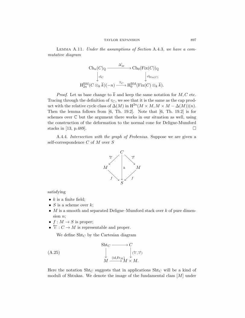
TAYLOR EXPANSION 897
Lemma A.11. Under the assumptions of Section A.4.3, we have a com-
mutative diagram
Chn(C)Q
clC
∆!M
// Ch0(Fix(C))Q
clFix(C)
HBM2n (C ⊗k k)(−n)
τC// HBM
0 (Fix(C)⊗k k).
Proof. Let us base change to k and keep the same notation for M,C etc.
Tracing through the definition of τC , we see that it is the same as the cap prod-
uct with the relative cycle class of ∆(M) in H2n(M ×M,M ×M −∆(M))(n).
Then the lemma follows from [6, Th. 19.2]. Note that [6, Th. 19.2] is for
schemes over C but the argument there works in our situation as well, using
the construction of the deformation to the normal cone for Deligne-Mumford
stacks in [13, p.489].
A.4.4. Intersection with the graph of Frobenius. Suppose we are given a
self-correspondence C of M over S
C
h
←−c
~~
−→c
M
f
M
f~~
S
satisfying
• k is a finite field;
• S is a scheme over k;
• M is a smooth and separated Deligne–Mumford stack over k of pure dimen-
sion n;
• f : M → S is proper;
• ←−c : C →M is representable and proper.
We define ShtC by the Cartesian diagram
ShtC //
C
(←−c ,−→c )
M(id,FrM )
// M ×M.
(A.25)
Here the notation ShtC suggests that in applications ShtC will be a kind of
moduli of Shtukas. We denote the image of the fundamental class [M ] under
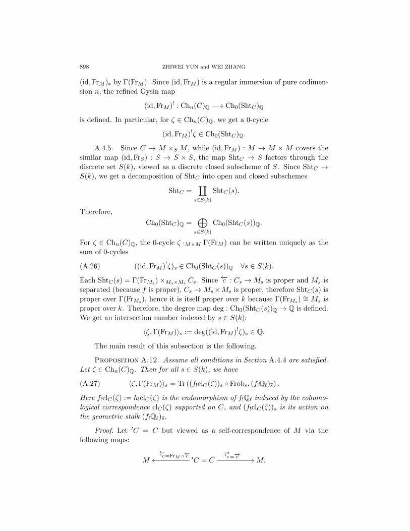
898 ZHIWEI YUN and WEI ZHANG
(id,FrM )∗ by Γ(FrM ). Since (id,FrM ) is a regular immersion of pure codimen-
sion n, the refined Gysin map
(id,FrM )! : Chn(C)Q −→ Ch0(ShtC)Q
is defined. In particular, for ζ ∈ Chn(C)Q, we get a 0-cycle
(id,FrM )!ζ ∈ Ch0(ShtC)Q.
A.4.5. Since C → M ×S M , while (id,FrM ) : M → M ×M covers the
similar map (id,FrS) : S → S × S, the map ShtC → S factors through the
discrete set S(k), viewed as a discrete closed subscheme of S. Since ShtC →S(k), we get a decomposition of ShtC into open and closed subschemes
ShtC =∐
s∈S(k)
ShtC(s).
Therefore,
Ch0(ShtC)Q =⊕
s∈S(k)
Ch0(ShtC(s))Q.
For ζ ∈ Chn(C)Q, the 0-cycle ζ ·M×M Γ(FrM ) can be written uniquely as the
sum of 0-cycles
(A.26) ((id,FrM )!ζ)s ∈ Ch0(ShtC(s))Q ∀s ∈ S(k).
Each ShtC(s) = Γ(FrMs)×Ms×Ms Cs. Since ←−c : Cs →Ms is proper and Ms is
separated (because f is proper), Cs →Ms×Ms is proper, therefore ShtC(s) is
proper over Γ(FrMs), hence it is itself proper over k because Γ(FrMs)∼= Ms is
proper over k. Therefore, the degree map deg : Ch0(ShtC(s))Q → Q is defined.
We get an intersection number indexed by s ∈ S(k):
〈ζ,Γ(FrM )〉s := deg((id,FrM )!ζ)s ∈ Q.
The main result of this subsection is the following.
Proposition A.12. Assume all conditions in Section A.4.4 are satisfied.
Let ζ ∈ Chn(C)Q. Then for all s ∈ S(k), we have
(A.27) 〈ζ,Γ(FrM )〉s = Tr ((f!clC(ζ))s Frobs, (f!Q`)s) .
Here f!clC(ζ) := h!clC(ζ) is the endomorphism of f!Q` induced by the cohomo-
logical correspondence clC(ζ) supported on C , and (f!clC(ζ))s is its action on
the geometric stalk (f!Q`)s.
Proof. Let ′C = C but viewed as a self-correspondence of M via the
following maps:
M ′C = C
←−′c=FrM ←−coo
−→′c=−→c// M.
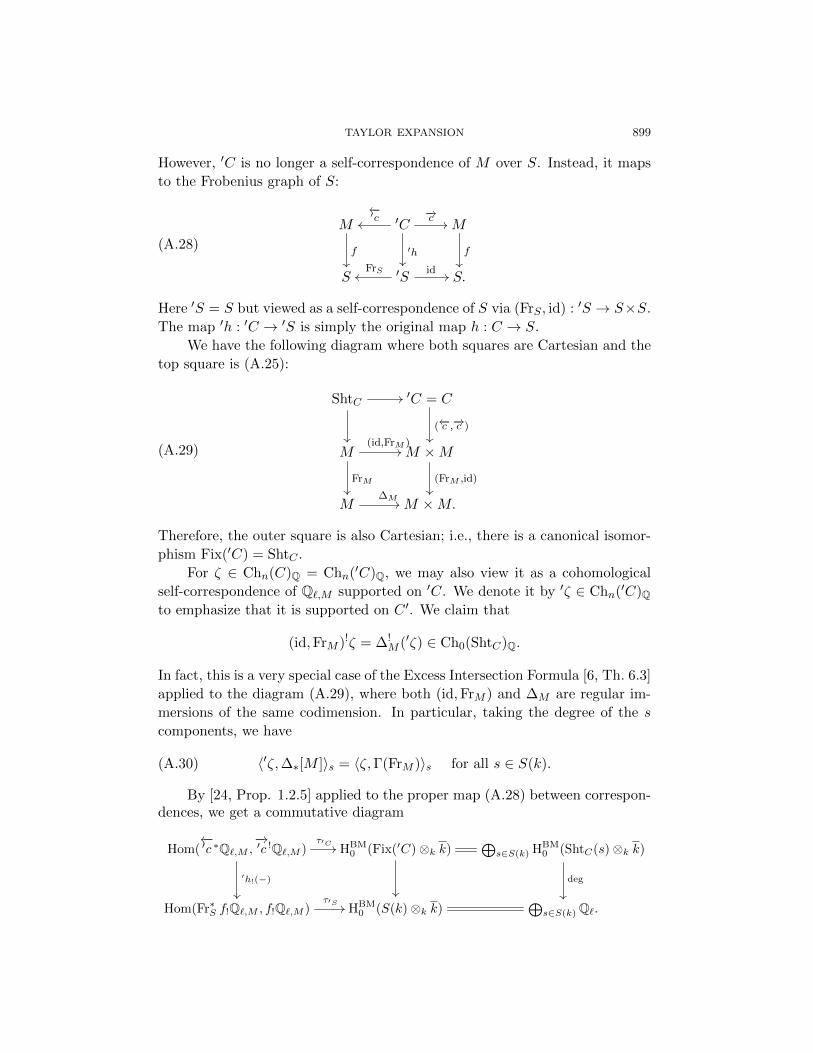
TAYLOR EXPANSION 899
However, ′C is no longer a self-correspondence of M over S. Instead, it maps
to the Frobenius graph of S:
M
f
′C
′h
←−′coo
−→c// M
f
S ′SFrSoo
id// S.
(A.28)
Here ′S = S but viewed as a self-correspondence of S via (FrS , id) : ′S → S×S.
The map ′h : ′C → ′S is simply the original map h : C → S.
We have the following diagram where both squares are Cartesian and the
top square is (A.25):
ShtC
// ′C = C
(←−c ,−→c )
M(id,FrM )
//
FrM
M ×M
(FrM ,id)
M∆M// M ×M.
(A.29)
Therefore, the outer square is also Cartesian; i.e., there is a canonical isomor-
phism Fix(′C) = ShtC .
For ζ ∈ Chn(C)Q = Chn(′C)Q, we may also view it as a cohomological
self-correspondence of Q`,M supported on ′C. We denote it by ′ζ ∈ Chn(′C)Qto emphasize that it is supported on C ′. We claim that
(id,FrM )!ζ = ∆!M (′ζ) ∈ Ch0(ShtC)Q.
In fact, this is a very special case of the Excess Intersection Formula [6, Th. 6.3]
applied to the diagram (A.29), where both (id,FrM ) and ∆M are regular im-
mersions of the same codimension. In particular, taking the degree of the s
components, we have
(A.30) 〈′ζ,∆∗[M ]〉s = 〈ζ,Γ(FrM )〉s for all s ∈ S(k).
By [24, Prop. 1.2.5] applied to the proper map (A.28) between correspon-dences, we get a commutative diagram
Hom(←−′c ∗Q`,M ,
−→′c !Q`,M )τ′C //
′h!(−)
HBM0 (Fix(′C)⊗k k)
⊕s∈S(k) HBM
0 (ShtC(s)⊗k k)
deg
Hom(Fr∗S f!Q`,M , f!Q`,M )τ′S // HBM
0 (S(k)⊗k k)⊕
s∈S(k) Q`.

900 ZHIWEI YUN and WEI ZHANG
Combining the with the commutative diagram in Lemma A.11 applied to ′C,
we get a commutative diagram
Chn(′C)Q∆!M
//
′h!cl′C
Ch0(Fix(′C))Q
⊕s∈S(k) Ch0(ShtC(s))
deg
Hom(Fr∗S f!Q`,M , f!Q`,M )τ′S// HBM
0 (S(k)⊗k k)⊕s∈S(k) Q`.
(A.31)
Applying (A.31) to ′ζ, and using (A.30), we get that for all s ∈ S(k),
(A.32) τ′SÄ′h!cl′C(′ζ)
äs
= 〈′ζ,∆∗[M ]〉s = 〈ζ,Γ(FrM )〉s.
Here τ′S(−)s ∈ Q` denotes the s-component of the class
τ′S(−) ∈ HBM0 (S(k)⊗k k) = ⊕s∈S(k)Q`.
Next we would like to express τ′SÄ′h!cl′C(′ζ)
äs
as a trace. The argument
works more generally when Q`,M is replaced with any F ∈ Dbc(M) and clC(ζ)
is replaced with any cohomological self-correspondence η : ←−c ∗F → −→c !F sup-
ported on C. So we will work in this generality. For any F ∈ Dbc(M), we have
a canonical isomorphism ΦF : Fr∗M F∼→ F whose restriction to the geometric
stalk at x ∈M(k) is given by the geometric Frobenius Frobx acting on Fx. A
similar remark applies to complexes on S. Using η we define a cohomological
self-correspondence ′η of F supported on ′C as the composition
′η :←−′c ∗F =←−c ∗ Fr∗M F
←−c ∗ΦF−−−−→←−c ∗F η−→ −→c !F =−→′c !F .
On the other hand we have a commutative diagram
(A.33) Fr∗S f!Fadj.
∼//
Φf!F
∼
%%
f! Fr∗M F
f!ΦFo
adj.// h!←−c ∗ Fr∗M F
h!←−c ∗ΦFo
h!
←−′c ∗F //
h!(′η)
f!F
f!Fadj.
// h!←−c ∗F
h!(η)// h!−→c !F
adj.// f!F .
Here the arrows indexed by “adj.” are induced from adjunctions, using the
properness of ←−c . The middle square is commutative by the definition of ′η,
and the right square is commutative by design. The composition of the top row
in (A.33) is by definition the push-forward ′h!′η as a cohomological self-corre-
spondence of f!F supported on ′S; the composition of the bottom row in (A.33)
is by definition the push-forward h!η as a cohomological self-correspondence of
f!F supported on the diagonal S. Therefore, (A.33) shows that ′h!′η may be
written as the composition
(A.34) ′h!′η : Fr∗S f!F
Φf!F−−−→ f!Fh!η−−→ f!F .

TAYLOR EXPANSION 901
For any cohomological self-correspondence ξ of G ∈ Dbc(S) supported on
the graph of Frobenius ′S, i.e., ξ : Fr∗S G → G, the trace τ′S(ξ)s at s ∈ S(k)
is simply given by the trace of ξs acting on the geometric stalk Gs: this is
because the Frobenius map is contracting at its fixed points, so the local term
for the correspondence supported on its graph is the naive local term (a very
special case of the main result in [24, Th. 2.1.3]). Applying this observation to
ξ = ′h!′η, we get
τ′S(′h!′η)s = Tr
Ä(′h!′η)s, (f!F)s
ä= Tr
Ä(h!η)s Frobs, (f!F)s
äby (A.34).
(A.35)
Now apply (A.35) to F = Q`,M , η = clC(ζ) and note that ′η = cl′C(′ζ). Then
(A.35) gives
τ′S(′h!cl′C(′ζ))s = TrÄ(f!clC(ζ))s Frobs, (f!Q`,M )s
ä.(A.36)
Combining (A.36) with (A.32) we get the desired formula (A.27).
Appendix B. Super-positivity of L-values
In this appendix we show the positivity of all derivatives of certain
L-functions (suitably corrected by their epsilon factors), assuming the Rie-
mann hypothesis. The result is unconditional in the function field case since
the Riemann hypothesis is known to hold.
It is well known that the positivity of the leading coefficient of such an
L-function is implied by the Riemann hypothesis. For nonleading terms, we
provisionally call such a phenomenon “super-positivity.”
Upon the completion of the paper, we learned that Stark and Zagier ob-
tained a result in [22] similar to our Proposition B.1.
B.1. The product expansion of an entire function. We recall the (canon-
ical) product expansion of an entire function following [1, §5.2.3, §5.3.2]. Let
φ(s) be an entire function in the variable s ∈ C. Let m be the vanishing order
of φ at s = 0. List all the nonzero roots of φ as α1, α2, . . . , αi, . . . (multiple
roots being repeated) indexed by a subset I of Z>0, such that |α1| ≤ |α2| ≤ · · · .Let En be the elementary Weierstrass function
En(u) =
(1− u) n = 0,
(1− u) eu+ 12u2+···+ 1
nun n ≥ 1.
An entire function φ is said to have finite genus if it can be written as an
absolutely convergent product
φ(s) = sm eh(s)∏i∈Z
En
Ås
αi
ã(B.1)

902 ZHIWEI YUN and WEI ZHANG
for a polynomial h(s) ∈ C[s] and an integer n ≥ 0. The product (B.1) is
unique if we further demand that n is the smallest possible integer, which is
characterized as the smallest n ∈ Z≥0 such that∑i∈I
1∣∣∣αi∣∣∣n+1 <∞.(B.2)
The genus g(φ) of such φ is then defined to be
g(φ) := maxdeg(h), n.
The order ρ(φ) of an entire function φ is defined as the smallest real number
ρ ∈ [0,∞] with the following property: for every ε > 0, there is a constant Cεsuch that ∣∣∣φ(s)
∣∣∣ ≤ e|s|ρ+ε , when |s| ≥ Cε.
If φ is a nonconstant entire function, an equivalent definition is
ρ(φ) = lim supr−→∞
log log ||φ||∞,Brr
,
where ||φ||∞,Br is the supremum norm of the function φ on the disc Br of
radius r. If the order of φ is finite, then Hadamard theorem [1, §5.3.2] asserts
that the function φ has finite genus and
g(φ) ≤ ρ(φ) ≤ g(φ) + 1.(B.3)
In particular, an entire function of finite order admits a product expansion of
the form (B.1).
The following result can be deduced from the proof in [22]. Since the proof
is very short, we include it for the reader’s convenience.
Proposition B.1. Let φ(s) be an entire function with the following prop-
erties :
(1) it has a functional equation φ(−s) = ±φ(s);
(2) for s ∈ R such that s 0, we have φ(s) ∈ R>0;
(3) the order ρ(φ) of φ(s) is at most 1;
(4) (RH) the only zeros of φ(s) lie on the imaginary axis Re(s) = 0.
Then for all r ≥ 0, we have
φ(r)(0) :=d
ds
∣∣∣∣s=0
φ(s) ≥ 0.
Moreover, if φ(s) is not a constant function, we have
φ(r0)(0) 6= 0 =⇒ φ(r0+2i)(0) 6= 0 for all r0 and i ∈ Z≥0.
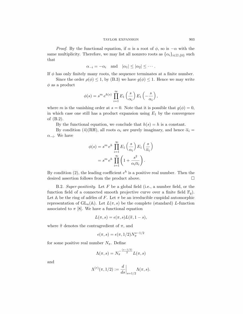
TAYLOR EXPANSION 903
Proof. By the functional equation, if α is a root of φ, so is −α with the
same multiplicity. Therefore, we may list all nonzero roots as αii∈Z\0 such
that
α−i = −αi and |α1| ≤ |α2| ≤ · · · .
If φ has only finitely many roots, the sequence terminates at a finite number.
Since the order ρ(φ) ≤ 1, by (B.3) we have g(φ) ≤ 1. Hence we may write
φ as a product
φ(s) = sm eh(s)∞∏i=1
E1
Ås
αi
ãE1
Å− s
αi
ã,
where m is the vanishing order at s = 0. Note that it is possible that g(φ) = 0,
in which case one still has a product expansion using E1 by the convergence
of (B.2).
By the functional equation, we conclude that h(s) = h is a constant.
By condition (4)(RH), all roots αi are purely imaginary, and hence αi =
α−i. We have
φ(s) = sm eh∞∏i=1
E1
Ås
αi
ãE1
Ås
αi
ã= sm eh
∞∏i=1
Ç1 +
s2
αiαi
å.
By condition (2), the leading coefficient eh is a positive real number. Then the
desired assertion follows from the product above.
B.2. Super-positivity. Let F be a global field (i.e., a number field, or the
function field of a connected smooth projective curve over a finite field Fq).Let A be the ring of adeles of F . Let π be an irreducible cuspidal automorphic
representation of GLn(A). Let L(π, s) be the complete (standard) L-function
associated to π [8]. We have a functional equation
L(π, s) = ε(π, s)L(π, 1− s),
where π denotes the contragredient of π, and
ε(π, s) = ε(π, 1/2)N s−1/2π
for some positive real number Nπ. Define
Λ(π, s) = N− (s−1/2)
2π L(π, s)
and
Λ(r)(π, 1/2) :=d
ds
∣∣∣∣s=1/2
Λ(π, s).
904 ZHIWEI YUN and WEI ZHANG
Theorem B.2. Let π be a nontrivial cuspidal automorphic representation
of GLn(A). Assume that it is self-dual :
π ' π.
Assume that, if F is a number field, then the Riemann hypothesis holds for
L(π, s); that is, all the roots of L(π, s) have real parts equal to 1/2.
(1) For all r ∈ Z≥0, we have
Λ(r)(π, 1/2) ≥ 0.
(2) If Λ(π, s) is not a constant function, we have
Λ(r0)(π, 1/2) 6= 0 =⇒ Λ(r0+2i)(π, 1/2) 6= 0 for all i ∈ Z≥0.
Proof. We consider
λ(π, s) := Λ(π, s+ 1/2).
Since π is cuspidal and nontrivial, its standard L-function L(π, s) is entire in
s ∈ C. By the equality ε(π, s)ε(π, 1 − s) = 1 and the self-duality π ' π we
deduce
1 = ε(π, 1/2)ε(π, 1− 1/2) = ε(π, 1/2)2.
Hence ε(π, 1/2) = ±1, and we have a functional equation
λ(π, s) = ±λ(π,−s).(B.4)
We apply Proposition B.1 to the entire function λ(π, s). The function L(π, s)
is entire of order one, and so is λ(π, s). In the function field case, condition
(4)(RH) is known by the theorem of Deligne on Weil conjecture, and of Drinfeld
and L. Lafforgue on the global Langlands correspondence. It remains to verify
condition (2) for λ(π, s). This follows from the following lemma.
The local L-factor L(πv, s) is of the form 1Pπv (q−sv )
, where Pπv is a polyno-
mial with constant term equal to one when v is nonarchimedean, and a product
of functions of the form ΓC(s+ α), or ΓR(s+ α), where α ∈ C, and
ΓC(s) = 2(2π)−sΓ(s), ΓR(s) = π−s/2Γ(s/2),
when v is archimedean. We say that L(πv, s) has real coefficients if the poly-
nomial Pπv has real coefficients when v is nonarchimedean, and the factor
ΓFv(s+ α) in L(πv, s) has real α or the pair ΓFv(s+ α) and ΓFv(s+ α) show
up simultaneously when v is archimedean. In particular, if L(πv, s) has real
coefficients, it takes positive real values when s is real and sufficiently large.
Lemma B.3. Let πv be unitary and self-dual. Then L(πv, s) has real co-
efficients.

TAYLOR EXPANSION 905
Proof. We suppress the index v in the notation and write F for a local
field. Let π be irreducible admissible representation of GLn(F ). It suffices to
show that, if π is unitary, then we have
L(π, s) = L(π, s).(B.5)
Let Zπ be the space of local zeta integrals, i.e., the meromorphic continuation of
Z(Φ, s, f) =
∫GLn(F )
f(g)Φ(g)|g|s+n−12 dg,
where f runs over all matrix coefficients of π, and Φ runs over all Bruhat–
Schwartz functions on Matn(F ) (a certain subspace, stable under complex
conjugation, if F is archimedean; cf. [8, §8]). We recall from [8, Th. 3.3, 8.7]
that the Euler factor L(π, s) is uniquely determined by the space Zπ. (For
instance, it is a certain normalized generator of the C[qs, q−s]-module Zπ if F
is nonarchimedean.)
Let Cπ be the space of matrix coefficients of π, i.e., the space consist-
ing of all linear combinations of functions on GLn(F ): g 7→ (π(g)u, v) where
u ∈ π, v ∈ π and (·, ·) : π× π → C is the canonical bilinear pairing. We remark
that the involution g 7→ g−1 induces an isomorphism between Cπ with Cπ.
To show (B.5), it now suffices to show that, if π is unitary, the complex
conjugation induces an isomorphism between Cπ and Cπ. Let 〈·, ·〉 : π×π → Cbe a nondegenerate Hermitian pairing invariant under GLn(F ). Then the space
Cπ consists of all functions fu,v : g 7→ 〈π(g)u, v〉, u, v ∈ π. Under complex con-
jugation we have fu,v(g) = 〈π(g)u, v〉 = 〈v, π(g)u〉 = 〈π(g−1)v, u〉 = fv,u(g−1).
This function belongs to Cπ by the remark at the end of the previous para-
graph. This clearly shows that the complex conjugation induces the desired
isomorphism.
Remark B.4. In the case of a function field, we have a simpler proof of
Theorem B.2. The function L(π, s) is a polynomial in q−s of degree denoted
by d. Then the function λ(π, s) is of the form
λ(π, s) = qds/2d∏i=1
Ä1− αiq−s
ä,(B.6)
where all the roots αi satisfy |αi| = 1. By the functional equation (B.4), if α is
a root in (B.6), so is α−1 = α. We divide all roots not equal to ±1 into pairs
α±11 , α±1
2 , . . . , α±1m (some of them may repeat). Consider
Ai(s) = qsÄ1− αiq−s
äÄ1− α−1
i q−sä
= qs + q−s − αi − αi
=Ä2− αi − αi
ä+ 2
∑j≥1
(s log q)2j
j!.

906 ZHIWEI YUN and WEI ZHANG
From |αi| = 1 and αi 6= 1 it follows that Ai(s) has strictly positive coefficients
at all even degrees. Now let a (resp., b) be the multiplicity of the root 1
(resp., −1). We then have
λ(π, s) =Äqs/2 − q−s/2
äa Äqs/2 + q−s/2
äb m∏i=1
Ai(s), 2m+ a+ b = d.
The desired assertions follow immediately from this product expansion.
Remark B.5. In the statement of the theorem, we excludes the trivial
representation. In this case the complete L-function has a pole at s = 1.
If we replace Λ(π, s) by s(s − 1)Λ(π, s), the theorem still holds by the same
proof. Moreover, if F = Q, we have the Riemann zeta function, and the super-
positivity is known without assuming the Riemann hypothesis, by Polya [4].
The super-positivity also holds when the L-function is “positive definite” as
defined by Sarnak in [21]. One of such examples is the weight 12 cusp form
with q-expansion ∆ = q∏n≥1(1 − qn)24. More recently, Goldfeld and Huang
in [9] prove that there are infinitely many classical holomorphic cusp forms
(Hecke eigenforms) on SL2(Z) whose L-functions satisfy super-positivity.
Remark B.6. The positivity of the central value is known for the standard
L-function attached to a symplectic cuspidal representation of GLn(A) by [16].
Remark B.7. The positivity of the first derivative is known for the L-
function appearing in the Gross–Zagier formula in [11], [27], for example the
L-function of an elliptic curve over Q.

Index
(·, ·)m, 774
(·, ·)π,λ, 774
(·, ·)π, 772
A, 776, 781
B,H, 850
C(hD), C(hD)d,d′ , 847
Dbc(S),DS , 781
F, F ′, 769
G = PGL2, 769
Grs,Ors, 782
H(hD), 813
HD, HD,D′ , 844
Hd, ‹Hd, 832
I ′d, 827
Ki, 869
Kx,K, 769
L(η, s), 775
L(π,Ad, s), 770
L(π, s), L(πF ′ , s), 770
L≤iV , 861
Ld, 793, 872
T , torus, 771, 816
V ′, 867
VQ` , VQ`,m, V′Q`,Eis, 773
W, W0, W , 772, 879
W [I],Wπ, λπ,mπ, 772
X,X ′, 769
Xd , 869
Xd, 789
Z′r0,`, 868
Zr0,`, 865
Zd, 790
ZEis, 798
Zcusp, 866
[A], 776, 783
[G] = G(F )\G(A), 781
[ShtT ]Eis, 868
A, 769
A1, 780
A×n , 783
Ir(f), 820
O, 769
Bun≤aG , 846
BunG, 809
BunT , 816
Bunn, 807
BunB ,BunB
, 850
Chc,i, 811
Chc,r, 771
Div(X), 780
FrS , 781
Γd, Sd, 869
GrLi V , 861
Hk′r,G,d,Hkµ,M♥,d, 834
Hk′rG,Hk′rG,d, 833
HkµG, 809
HkrG, 811
Hkµ,dB
, 850
HkµT , 817
HkµM,d, Hkµ
M,d, 825
HkµM♦,d, 826
HkµM♥,d, 831, 834
Hkµn, 808
Hkr,G,d, 834
HkrG,d,Hkµ2,d, 833
Π, 819
PicdX , 789
PrymX′/X , 823
Sat, Satx, 797
Sht′rG,d, 831, 837
Sht′rG, 771, 820
ShtµG, 809, 811
ShtrG, 811
Sht≤dG , 846
Shtµ,dB
, 850
ShtµT , 771, 817
ShtµM,D, 829
ShtµM,d, 828
ShtµM,d(a), 829
ShtµM♥,d, 832
ShtµT
, 816
ShtdB , 851
ShtdG, 846
ShtdH , 852
ShtrG,d, 836
ShtrG(hD), 812
Shtµn, 808
Σd, d, 789
H`′, 867
cCh2r, 811
907

908 ZHIWEI YUN and WEI ZHANG
A,Aπ, 769
Ad, 790
AD, 793
A♥d , 790
A♦d , 826, 870
D, 846
D+, 852
Dn,D≤n, 863
H = Hk1M,d, 826
H♦, 826, 870
IEis, 772, 798
Ki,K′i, 789
M♦d , 826, 870
M♥d , 831, 832
Nd, 872
Ox, Fx, kx, 769
cl, cycle class, 849
H∗(S ⊗k k),H∗c(S ⊗k k), 781
δ : Ad → “Xd, 790
Ir(π, f), 777
Ir(f), 776
Ir(u, hD), 828, 872
J(γ, f, s), 785
J(f, s), 776, 783
J(u, f, s), 787
Jπ(f, s), 776, 803
Jr(γ, f), 786
Jr(f), 776, 786
Jr(u, f), 787
Jn1,n2(γ, f, s), 784
Jn1,n2(f, s), 783, 784
Kf , 783, 784
Kf,γ , 784
Kf,π, 800
Kf,Eis, 801
Kf,cusp, 800
Kf,sp, 800
Pχ(φ, s), 802
ε(πF ′ , s), 770
ηF ′/F , 769
γ, γ(u), 782
γd, γδ, 857“Xd, 789
H∗(S ⊗k k),HBM∗ (S ⊗k k), 781
inst(E), 846
inv, 782
invD, 793≤dShtG(hD), 847
µ, µ±, 807
ν : X ′ → X, 769←−p ,−→p , 812
ωX , 772, 806
H`, 863
∂HkµM♦,d, 842
π,Eπ, 769
π≤dG , π<dG , πdG, 847
πµT , 771, 817
πµn, 808
πG, 771, 811
H , Hecke algebra, 769, 788, 797
HA,HA,x, 797
HH , 857
Hx, hnx, hD, 788, 797
HEis, 798
Haut,Haut,Q` , 866
Hcusp, 866
L (πF ′ , s), 770
L (r)(πF ′ , 1/2), 770
sgn(µ), 807
σ : X ′ → X ′, 769
τ≤i, 860
Ad, 826
Md,Md, 821‹Nd,Nd, 789
fM, 826
θµ, 771, 820
θµ∗ [ShtµT ], 771, 820›H`, 875
val, 780
$x,Ox, kx, dx, qx, 780
addd1,d2 , addd1,d2 , 789
νd, 821
ND,γ
,ND,γ
, 794
T , 816
ζ♥, 830
ζF , ζx, 780τE , 808
aEis, 798
f ∗ (−), 814
fM, 821
fNd , 790
g, g′, 769
k = Fq, 769
n±, w, 782
TAYLOR EXPANSION 909
References
[1] L. V. Ahlfors, Complex Analysis : An Introduction of the Theory of Analytic
Functions of One Complex Variable, Second edition, McGraw-Hill Book Co., New
York, 1966. MR 0188405. Zbl 0154.31904.
[2] K. Behrend and B. Fantechi, The intrinsic normal cone, Invent. Math. 128
no. 1 (1997), 45–88. MR 1437495. Zbl 0909.14006. https://doi.org/10.1007/
s002220050136.
[3] A. A. Beılinson, J. Bernstein, and P. Deligne, Faisceaux pervers, in Anal-
ysis and Topology on Singular Spaces, I (Luminy, 1981), Asterisque 100, Soc.
Math. France, Paris, 1982, pp. 5–171. MR 0751966. Zbl 0536.14011.
[4] G. Csordas, T. S. NSorfolk, and R. S. Varga, The Riemann hypothesis
and the Turan inequalities, Trans. Amer. Math. Soc. 296 no. 2 (1986), 521–541.
MR 0846596. Zbl 0602.30030. https://doi.org/10.2307/2000378.
[5] V. G. Drinfel′d, Moduli varieties of F -sheaves, Funktsional. Anal. i Prilozhen.
21 no. 2 (1987), 23–41. MR 0902291. Zbl 0665.12013.
[6] W. Fulton, Intersection Theory, second ed., Ergeb. Math. Grenzgeb. 2, Springer-
Verlag, Berlin, 1998. MR 1644323. Zbl 0885.14002. https://doi.org/10.1007/
978-1-4612-1700-8.
[7] H. Gillet, Intersection theory on algebraic stacks and Q-varieties, in Proceedings
of the Luminy Conference on Algebraic K-Theory (Luminy, 1983), 34 J. Pure
Appl. Algebra no. 2-3, 1984, pp. 193–240. MR 0772058. Zbl 0607.14004. https:
//doi.org/10.1016/0022-4049(84)90036-7.
[8] R. Godement and H. Jacquet, Zeta Functions of Simple Algebras, Lecture
Notes in Math. 260, Springer-Verlag, New York, 1972. MR 0342495. Zbl 0244.
12011.
[9] D. Goldfeld and B. Huang, Super-positivity of a family of L-functions, 2016,
preprint. arXiv 1612.09359.
[10] M. Goresky and R. MacPherson, Intersection homology. II, Invent. Math.
72 no. 1 (1983), 77–129. MR 0696691. Zbl 0529.55007. https://doi.org/10.1007/
BF01389130.
[11] B. H. Gross and D. B. Zagier, Heegner points and derivatives of L-series,
Invent. Math. 84 no. 2 (1986), 225–320. MR 0833192. Zbl 0608.14019. https:
//doi.org/10.1007/BF01388809.
[12] H. Jacquet, Sur un resultat de Waldspurger, Ann. Sci. Ecole Norm. Sup. (4)
19 no. 2 (1986), 185–229. MR 0868299. Zbl 0605.10015. Available at http://
www.numdam.org/item?id=ASENS 1986 4 19 2 185 0.
[13] A. Kresch, Canonical rational equivalence of intersections of divisors, Invent.
Math. 136 no. 3 (1999), 483–496. MR 1695204. Zbl 0923.14003. https://doi.
org/10.1007/s002220050317.
[14] A. Kresch, Cycle groups for Artin stacks, Invent. Math. 138 no. 3 (1999), 495–
536. MR 1719823. Zbl 0938.14003. https://doi.org/10.1007/s002220050351.
[15] V. Lafforgue, Chtoucas pour les groupes reductifs et parametrisation de lang-
lands globale, 2012. arXiv 1209.5352.
910 ZHIWEI YUN and WEI ZHANG
[16] E. Lapid and S. Rallis, On the nonnegativity of L( 12 , π) for SO2n+1, Ann. of
Math. (2) 157 no. 3 (2003), 891–917. MR 1983784. Zbl 1067.11026.
[17] Y. Laszlo and M. Olsson, The six operations for sheaves on Artin stacks. II.
Adic coefficients, Publ. Math. Inst. Hautes Etudes Sci. no. 107 (2008), 169–210.
MR 2434693. Zbl 1191.14003. https://doi.org/10.1007/s10240-008-0012-5.
[18] G. Laumon, Correspondance de Langlands geometrique pour les corps de fonc-
tions, Duke Math. J. 54 no. 2 (1987), 309–359. MR 0899400. Zbl 0662.12013.
https://doi.org/10.1215/S0012-7094-87-05418-4.
[19] B. C. Ngo, Fibration de Hitchin et endoscopie, Invent. Math. 164 no. 2
(2006), 399–453. MR 2218781. Zbl 1098.14023. https://doi.org/10.1007/
s00222-005-0483-7.
[20] B. C. Ngo, Le lemme fondamental pour les algebres de Lie, Publ. Math. Inst.
Hautes Etudes Sci. no. 111 (2010), 1–169. MR 2653248. Zbl 1200.22011. https:
//doi.org/10.1007/s10240-010-0026-7.
[21] P. Sarnak, Letter to E. Bachmat on positive definite L-functions, 2011.
[22] H. M. Stark and D. Zagier, A property of L-functions on the real line, J.
Number Theory 12 no. 1 (1980), 49–52. MR 0566867. Zbl 0428.10021. https:
//doi.org/10.1016/0022-314X(80)90071-2.
[23] Y. Varshavsky, Moduli spaces of principal F -bundles, Selecta Math. (N.S.) 10
no. 1 (2004), 131–166. MR 2061225. Zbl 1070.14026. https://doi.org/10.1007/
s00029-004-0343-0.
[24] Y. Varshavsky, Lefschetz-Verdier trace formula and a generalization of a the-
orem of Fujiwara, Geom. Funct. Anal. 17 no. 1 (2007), 271–319. MR 2306659.
Zbl 1131.14019. https://doi.org/10.1007/s00039-007-0596-9.
[25] A. Vistoli, Intersection theory on algebraic stacks and on their moduli spaces,
Invent. Math. 97 no. 3 (1989), 613–670. MR 1005008. Zbl 0694.14001. https:
//doi.org/10.1007/BF01388892.
[26] J.-L. Waldspurger, Sur les valeurs de certaines fonctions L automorphes en
leur centre de symetrie, Compositio Math. 54 no. 2 (1985), 173–242. MR 0783511.
Zbl 0567.10021. Available at http://www.numdam.org/item?id=CM 1985 54
2 173 0.
[27] X. Yuan, S.-W. Zhang, and W. Zhang, The Gross-Zagier Formula on Shimura
Curves, Ann. of Math. Stud. 184, Princeton Univ. Press, Princeton, NJ, 2013.
MR 3237437. Zbl 1272.11082.
[28] Z. Yun, An arithmetic fundamental lemma for function fields, 2011, preprint.
[29] Z. Yun, The fundamental lemma of Jacquet and Rallis, Duke Math. J. 156 no. 2
(2011), 167–227, With an appendix by Julia Gordon. MR 2769216. Zbl 1211.
14039. https://doi.org/10.1215/00127094-2010-210.
[30] W. Zhang, On arithmetic fundamental lemmas, Invent. Math. 188 no. 1
(2012), 197–252. MR 2897697. Zbl 1247.14031. https://doi.org/10.1007/
s00222-011-0348-1.
[31] W. Zhang, Automorphic period and the central value of Rankin-Selberg L-
function, J. Amer. Math. Soc. 27 no. 2 (2014), 541–612. MR 3164988. Zbl 1294.
11069. https://doi.org/10.1090/S0894-0347-2014-00784-0.
TAYLOR EXPANSION 911
(Received: January 7, 2016)
(Revised: January 23, 2017)
Yale University, New Haven, CT
E-mail : [email protected]
Columbia University, New York, NY
E-mail : [email protected]