9. The Relativistic Topology

9.1  In the Neighborhood 

Nothing puzzles me more than time and space; and yet nothing troubles me less, as I never think about them.                                                                    Charles Lamb (1775-1834)

 It's customary to treat the relativistic spacetime manifold as an ordinary topological space with the same topology as a four-dimensional Euclidean manifold, denoted by R4.  This is typically justified by noting that the points of spacetime can be parameterized by a set of four coordinates x,y,z,t, and defining the "neighborhood" of a point somewhat informally as follows (quoted from Ohanian and Ruffinni): 

...the neighborhood of a given point is the set of all points such that their coordinates differ only a little from those of the given point.

 Of course, the neighborhoods given by this definition are not Lorentz-invariant, because the amount by which the coordinates of two points differ is highly dependent on the frame of reference.  Consider, for example, two spacetime points in the xt plane with the coordinates {0,0} and {1,1} with respect to a particular system of inertial coordinates.  If we consider these same two points with respect to the frame of an observer moving in the positive x direction with speed v (and such that the origin coincides with the former coordinate origin), the differences in both the space and time coordinates are reduced by

a factor of , which can range anywhere between 0 and  .  Thus there exist valid inertial reference systems with respect to which both of the coordinates of these points differ (simultaneously) by as little or as much as we choose.  Based on the above definition of neighborhood (i.e., points whose coordinates “differ only a little”), how can we decide if these two points are in the same neighborhood? It might be argued that the same objection could be raised against this coordinate-based definition of neighborhoods in Euclidean space, since we're free to scale our coordinates arbitrarily, which implies that the numerical amount by which the coordinates of two given (distinct) points differ is arbitrary.  However, in Euclidean space this objection is unimportant, because we will arrive at the same definition of limit points, and thus the same topology, regardless of what scale factor we choose.  In fact, the same applies even if we choose unequal scale factors in different directions, provided those scale factors are all finite and non-zero.   From a strictly mathematical standpoint, the usual way of expressing the arbitrariness of metrical scale factors for defining a topology on a set of points is to say that if two systems of coordinates are related by a diffeomorphism (a differentiable mapping that possess a differentiable inverse), then the definition of neighborhoods in terms of "coordinates that differ only a little" will yield the same limit points and thus the same topology.  However, from the standpoint of a physical theory it's legitimate to ask whether the set of distinct points (i.e., labels) under our chosen coordinate system

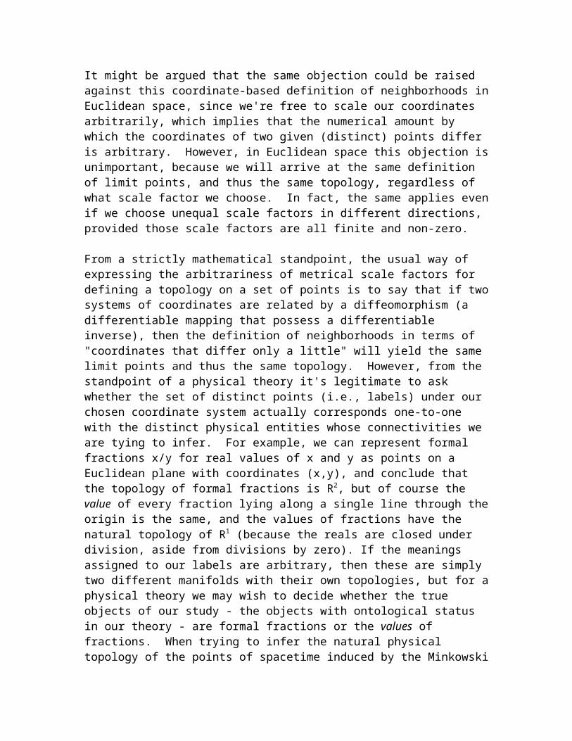
actually corresponds one-to-one with the distinct physical entities whose connectivities we are tying to infer.  For example, we can represent formal fractions x/y for real values of x and y as points on a Euclidean plane with coordinates (x,y), and conclude that the topology of formal fractions is R2, but of course the value of every fraction lying along a single line through the origin is the same, and the values of fractions have the natural topology of R1 (because the reals are closed under division, aside from divisions by zero). If the meanings assigned to our labels are arbitrary, then these are simply two different manifolds with their own topologies, but for a physical theory we may wish to decide whether the true objects of our study - the objects with ontological status in our theory - are formal fractions or the values of fractions.  When trying to infer the natural physical topology of the points of spacetime induced by the Minkowski metric we face a similar problem of identifying the actual physical entities whose mutual connectivities we are trying to infer, and the problem is complicated by the fact that the "Minkowski metric" is not really a metric at all (as explained below). Recall that for many years after general relativity was first proposed by Einstein there was widespread confusion and misunderstanding among leading scientists (including Einstein himself) regarding various kinds of singularities. The main source of confusion was the failure to clearly distinguish between singularities of coordinate systems as opposed to actual singularities of the manifold/field. This illustrates how we can be misled by the belief that the local topology of a physical manifold corresponds to the local topology of any particular system of coordinates that we may assign to that physical manifold. It’s entirely possible for the “manifold of coordinates” to have a different topology than the physical manifold to which those coordinates are applied. With this in mind, it’s worthwhile to consider carefully whether the most physically meaningful local topology of spacetime is necessarily the same as the topology of the usual four-dimensional systems of coordinates that are conventionally applied to it. Before examining the possible topologies of Minkowski spacetime in detail, it's worthwhile to begin with a review of the basic definitions of point set topologies and topological spaces.  Given a set S, let P(S) denote the set of all subsets of S.  A topology for the set S is a mapping T from the Cartesian product {S P(S)} to the discrete set {0,1}.  In other words, given any element e of S, and any subset A of S, the mapping T(A,e) returns either 0 or 1.  In the usual language of topology, we say that e is a limit point of A if and only if T(A,e) = 1. As an example, we can define a topology on the set of points of 2D Euclidean space equipped with the usual Pythagorean metric  

                                (1) by saying that the point e is a limit point of any subset A of points of the plane if and only if for every positive real number there is an element u (other than e) of A such that d(e,u) < .  Clearly this definition relies on prior knowledge of the "topology" of the real numbers, which is denoted by R1.  The topology of 2D Euclidean space is called R2, since it is just the Cartesian product R1 R1. 

 The topology of a Euclidean space described above is actually a very special kind of topology, called a topological space.  The distinguishing characteristic of a topological space S,T is that S contains a collection of subsets, called the open sets (including S itself and the empty set) which is closed under unions and finite intersections, and such that a point p is a limit point of a subset A of S if and only if every open set containing p also contains a point of A distinct from p.  For example, if we define the collection of open spherical regions in Euclidean space, together with any regions that can be formed by the union or finite intersection of such spherical regions, as our open sets, then we arrive at the same definition of limit points as given previously.  Therefore, the topology we've described for the points of Euclidean space constitutes a topological space.  However, it's important to realize that not every topology is a topological space. The basic sets that we used to generate the Euclidean topology were spherical regions defined in terms of the usual Pythagorean metric, but the same topology would also be generated by any other metric.  In general, a basis for a topological space on the set S is a collection B of subsets of S whose union comprises all of S and such that if p is in the intersection of two elements Bi and Bj of B, then there is another element Bk of B which contains p and which is entirely contained in the intersection of Bi and Bj, as illustrated below for circular regions on a plane. 

 Given a basis B on the set S, the unions of elements of B satisfy the conditions for open sets, and hence serve to define a topological space.  (This relies on the fact that we can represent non-circular regions, such as the intersection of two circular open sets, as the union of an infinite number of circular regions of arbitrary sizes.) If we were to substitute the metric  

d(a,b)  =  |xa xb|  +  |ya yb|  in place of the Pythagorean metric, then the basis sets, defined as loci of points whose "distances" from a fixed point p are less than some specified real number r, would be square-shaped diamonds instead of circles, but we would arrive at the same topology, i.e., the same definition of limit points for the subsets of the Euclidean plane E2.  In general, any true metric will induce this same local topology on a manifold.  Recall that a metric is defined as a distance function d(a,b) for any two points a,b in the space satisfying the three axioms 

                        (1)  d(a,b) = 0   if and only if a = b                        (2)  d(a,b) = d(b,a)   for each a,b                        (3)  d(a,c) d(a,b) + d(b,c)   for all a,b,c It follows that d(a,b) 0 for all a,b.  Any distance function that satisfies the conditions of a metric will induce the same (local) topology on a set of points, and this will be a topological space. However, it's possible to conceive of more general "distance functions" that do not satisfy all the axioms of a metric.  For example, we can define a distance function that is commutative (axiom 2) and satisfies the triangle inequality (axiom 3), but that allows d(a,b) = 0 for distinct points a,b.  Thus we replace axiom (1) with the weaker requirement d(a,a) = 0.  Such a distance function is called a pseudometric.  Obviously if a,b are any two points with d(a,b) = 0 we must have d(a,c) = d(b,c) for every point c, because otherwise the points a,b,c would violate the triangle inequality.  Thus a pseudometric partitions the points of the set into equivalence classes, and the distance relations between these equivalence classes must be metrical.  We've already seen a situation in which a pseudometric arises naturally, if we define the distance between two points in the plane of formal fractions as the absolute value of the difference in slopes of the lines from the origin to those two points.  The distance between any two points on a single line through the origin is therefore zero, and these lines represent the equivalence classes induced by the pseudometric.  Of course, the distances between the slopes satisfy the requirements of a metric.  Therefore, the absolute difference of value is a pseudometric for the space of formal fractions.   Now, we know that the points of a two-dimensional plane can be assigned the R2 topology, and the values of fractions can be assigned the R1 topology, but what kind of local topology is induced on the two-dimensional space of formal fractions by the pseudometric?  We can use our pseudometric distance function to define a basis, just as with a metrical distance function, and arrive at a topological space, but this space will not generally possess all the separation properties that we commonly expect for distinct points of a topological space.   It's convenient to classify the separation properties of topological spaces according to the "trennungsaxioms", also called the Ti axioms, introduced by Alexandroff and Hopf.  These represent a sequence of progressively stronger separation axioms to be met by the points of a topological space.  A space is said to be T0 if for any two distinct points at least one of them is in a neighborhood that does not include the other.  If each point is contained in a neighborhood that does not include the other, then the space is called T1.  If the space satisfies the even stronger condition that any two points are contained in disjoint open sets, then the space is called T2, also known as a Hausdorff space.  There are still more stringent separation axioms that can be applied, corresponding to T3 (regular), T4 (normal), and so on. Many topologists will not even consider a topological space which is not at least T2 (and some aren't interested in anything which is not at least T4), and yet it's clear that the

topology of the space of formal fractions induced by the pseudometric of absolute values is not even T0, because two distinct fractions with the same value (such as 1/3 and 2/6) cannot be separated into different neighborhoods by the pseudometric.  Nevertheless, we can still define the limit points of the set of formal fractions based on the pseudometric distance function, thereby establishing a perfectly valid topology.  This just illustrates that the distinct points of a topology need not exhibit all the separation properties that we usually associate with distinct points of a Hausdorff spaces (for example). Now let's consider 1+1 dimensional Minkowski spacetime, which is physically characterized by an invariant spacetime interval whose magnitude is 

d(a,b)   =   | (ta tb)2    (xa xb)2 |                                           (2) Empirically this appears to be the correct measure of absolute separation between the points of spacetime, i.e., it corresponds to what clocks measure along timelike intervals and what rulers measure along spacelike intervals.  However, this distance function clearly does not satisfy the definition of a metric, because it can equal zero for distinct points.  Moreover, it is not even a pseudo-metric, because the interval between points a and b is always greater than the sum of the intervals from a to c and from c to b, contradicting the triangle inequality.  For example, it's quite possible in Minkowski spacetime to have two sides of a "triangle" equal to zero while the remaining side is billions of light years in length.  Thus, the absolute interval of space-time does not provide a metrical measure of distance in the strict sense.  Nevertheless, in other ways the magnitude of the interval d(a,b) is quite analogous to a metrical distance, so it's customary to refer to it loosely as a "metric", even though it is neither a true metric nor even a pseudometric.  We emphasize this fact to remind ourselves not to prejudge the topology induced by this distance function on the points of Minkowski spacetime, and not to assume that distinct events possess the separation properties or connectivities of a topological space. The -neighborhood of a point p in the Euclidean plane based on the Pythagorean metric (1) consists of the points q such that d(p,q) < .   Thus the -neighborhoods of two points in the plane are circular regions centered on the respective points, as shown in the left-hand illustration below.  In contrast, the -neighborhoods of two points in Minkowski spacetime induced by the Lorentz-invariant distance function (2) are the regions bounded by the hyperbolic envelope containing the light lines emanating from those points, as shown in the right-hand illustration below.

 This illustrates the important fact that the concept of "nearness" implied by the Minkowski metric is non-transitive.  In a metric (or even a pseudometric) space, the triangle inequality ensures that if A and B are close together, and B and C are close together, then A and C cannot be very far apart.  This transitivity obviously doesn't apply to the absolute magnitudes of the spacetime intervals between events, because it's possible for A and B to be null-separated, and for B and C to be null separated, while A and C are arbitrarily far apart. Interestingly, it is often suggested that the usual Euclidean topology of spacetime might break down on some sufficiently small scale, such as over distances on the order of the Planck length of roughly 10-35 meters, but the system of reference for evaluating that scale is usually not specified.  As noted previously, the spatial and temporal components of two null-separated events can both simultaneously be regarded as arbitrarily large or arbitrarily small (including less than 10-35 meters), depending on which system of inertial coordinates we choose.  This null-separation condition permeates the whole of spacetime (recall Section 1.10 on Null Coordinates), so if we take seriously the possibility of non-Euclidean topology on the Planck scale, we can hardly avoid considering the possibility that the effective physical topology ("connectedness") of the points of spacetime may be non-Euclidean along null intervals in their entirety, which span all scales of spacetime. It's certainly true that the topology induced by a direct application of the Minkowski distance function (2) is not even a topological space, let alone Euclidean.  To generate this topology, we simply say that  the point e is a limit point of any subset A of points of Minkowski spacetime if and only if for every positive real number there is an element u (other than e) of A such that d(e,u) < .   This is a perfectly valid topology, and arguably the one most consistent with the non-transitive absolute intervals that seem to physically characterize spacetime, but it is not a topological space.  To see this, recall that in order for a topology to be a topological space it must be possible to express the limit point mapping in terms of open sets such that a point e is a limit point of a subset A of S if and only if every open set containing e also contains a point of A distinct from e.  If we define

our topological neighborhoods in terms of the Minkowski absolute intervals, our open sets would naturally include complete Minkowski neighborhoods, but these regions don't satisfy the condition for a topological space, as illustrated below, where e is a limit point of A, but e is also contained in Minkowski neighborhoods containing no point of A. 

The idea of a truly Minkowskian topology seems unsatisfactory to many people, because they worry that it implies every two events are mutually "co-local" (i.e., their local neighborhoods intersect), and so the entire concept of "locality" becomes meaningless.  However, the fact that a set of points possesses a non-positive-definite line element does not imply that the set degenerates into a featureless point  (which is fortunate, considering that the spacetime we inhabit is characterized by just such a line element).  It simply implies that we need to apply a more subtle understanding of the concept of locality, taking account of its non-transitive aspect.  In fact, the overlapping of topological neighborhoods in spacetime suggests a very plausible approach to explaining the "non-local" quantum correlations that seem so mysterious when viewed from the viewpoint of Euclidean topology.   We'll consider this in more detail in subsequent chapters. It is, of course, possible to assign the Euclidean topology to Minkowski spacetime, but only by ignoring the non-transitive null structure implied by the Lorentz-invariant distance function.  To do this, we can simply take as our basis sets all the finite intersections of Minkowski neighborhoods.  Since the contents of an -neighborhood of a given point are invariant under Lorentz transformations, it follows that the contents of the intersection of the -neighborhoods of two given points are also invariant.  Thus we can define each basis set by specifying a finite collection of events with a specific value of for each one, and the resulting set of points is invariant under Lorentz transformations.  This is a more satisfactory approach than defining neighborhoods as the set of points whose coordinates (with respect to some arbitrary system of coordinates) differ only a little, but the fact remains that by adopting this approach we are still tacitly abandoning the Lorentz-invariant sense of nearness and connectedness, because we are segregating

null-separated events into disjoint open sets.  This is analogous to saying, for the plane of formal fractions, that 4/6 is not a limit point of every set containing 2/3, which is certainly true on the formal level, but it ignores the natural topology possessed by the values of fractions.  In formulating a physical theory of fractions we would need to decide at some point whether the observable physical phenomena actually correspond to pairings of numerators and denominators, or to the values of fractions, and then select the appropriate topology.  In the case of a spacetime theory, we need to consider whether the temporal and spatial components of intervals have absolute significance, or whether it is only the absolute intervals themselves that are significant. It's worth reviewing why we ever developed the Euclidean notion of locality in the first place, and why it's so deeply engrained in our thought processes, when the spacetime which we inhabit actually possesses a Minkowskian structure.  This is easily attributed to the fact that our conscious experience is almost exclusively focused on the behavior of macro-objects whose overall world-lines are nearly parallel relative to the characteristic of the metric.  In other words, we're used to dealing with objects whose mutual velocities are small relative to c, and for such objects the structure of spacetime does approach very near to being Euclidean.  On the scales of space and time relevant to macro human experience the trajectories of incoming and outgoing light rays through any given point are virtually indistinguishable, so it isn't surprising that our intuition reflects a Euclidean topology.  (Compare this with the discussion of Postulates and Principles in Chapter 3.1.) Another important consequence of the non-positive-definite character of Minkowski spacetime concerns the qualitative nature of geodesic paths.  In a genuine metric space the geodesics are typically the shortest paths from place to place, but in Minkowski spacetime the timelike geodesics are the longest paths, in terms of the absolute value of the invariant intervals.  Of course, if we allow curvature, there may be multiple distinct "maximal" paths between two given events.  For example, if we shoot a rocket straight up (with less than escape velocity), and it passes an orbiting satellite on the way up, and passes the same satellite again on the way back down, then each of them has followed a geodesic path between their meetings, but they have followed very different paths. From one perspective, it's not surprising that the longest paths in spacetime correspond to physically interesting phenomena, because the shortest path between any two points in Minkowski spacetime is identically zero.  Hence the structure of events was bound to involve the longest paths.  However, it seems rash to conclude that the shortest paths play no significant role in physical phenomena.  The shortest absolute timelike path between two events follows a "dog leg" path, staying as close as possible to the null cones emanating from the two events.  Every two points in spacetime are connected by a contiguous set of lightlike intervals whose absolute magnitudes are zero. Minkowski spacetime provides an opportunity to reconsider the famous "limit paradox" from freshman calculus in a new context.  Recall the standard paradox begins with a two-part path in the xy plane from point A to point C by way of point B as shown below: 

If the real segment AC has length 1, then the dog-leg path ABC has length , as does each of the zig-zag paths ADEFC, AghiEjklC, and so on.  As we continue to subdivide the path into more and smaller zigzags the envelope of the path converges on the straight line from A to C.  The "paradox" is that the limiting zigzag path still has length , whereas the line to which it converges (and from which we might suppose it is indistin-guishable) has length 1.  Needless to say, this is not a true paradox, because the limit of a set of convergents does not necessarily possess all the properties of the convergents.  However, from a physical standpoint it teaches a valuable lesson, which is that we can't necessarily assess the length of a path by assuming it equals the length of some curve from which it never differs by any measurable amount. To place this in the context of Minkowski spacetime, we can simply replace the y axis with the time axis, and replace the Euclidean metric with the Minkowski pseudo-metric. We can still assume the length of the interval AC is 1, but now each of the diagonal segments is a null interval, so the total path length along any of the zigzag paths is identically zero.  In the limit, with an infinite number of infinitely small zigzags, the jagged "null path" is everywhere practically coincident with the timelike geodesic path AC, and yet its total length remains zero.  Of course, the oscillating acceleration required to propel a massive particle on a path approaching these light-like segments would be enormous, as would the frequency of oscillation. 9.2  Up To Diffeomorphism 

The mind of man is more intuitive than logical, and comprehends more than it can coordinate.                                                                                                Vauvenargues, 1746

 

Einstein seems to have been strongly wedded to the concept of the continuum described by partial differential equations as the only satisfactory framework for physics. He was certainly not the first to hold this view. For example, in 1860 Riemann wrote 

As is well known, physics became a science only after the invention of differential calculus. It was only after realizing that natural phenomena are continuous that attempts to construct abstract models were successful… In the first period, only certain abstract cases were treated: the mass of a body was considered to be concentrated at its center, the planets were mathematical points… so the passage from the infinitely near to the finite was made only in one variable, the time [i.e., by means of total differential equations]. In general, however, this passage has to be done in several variables… Such passages lead to partial differential equations… In all physical theories, partial differential equations constitute the only verifiable basis. These facts, established by induction, must also hold a priori. True basic laws can only hold in the small and must be formulated as partial differential equations.

 Compare this with Einstein’s comments (see Section 3.2) over 70 years later about the unsatisfactory dualism inherent in Lorentz’s theory, which expressed the laws of motion of particles in the form of total differential equations while describing the electromagnetic field by means of partial differential equations. Interestingly, Riemann asserted that the continuous nature of physical phenomena was “established by induction”, but immediately went on to say it must also hold a priori, referring somewhat obscurely to the idea that “true basic laws can only hold in the infinitely small”. He may have been trying to convey by these words his rejection of “action at a distance”. Einstein attributed this insight to the special theory of relativity, but of course the Newtonian concept of instantaneous action at a distance had always been viewed skeptically, so it isn’t surprising that Riemann in 1860 – like his contemporary Maxwell – adopted the impossibility of distant action as a fundamental principle. (It’s interesting the consider whether Einstein might have taken this, rather than the invariance of light speed, as one of the founding principles of special relativity, since it immediately leads to the impossibility of rigid bodies, etc.) In his autobiographical notes (1949) Einstein wrote 

There is no such thing as simultaneity of distant events; consequently, there is also no such thing as immediate action at a distance in the sense of Newtonian mechanics. Although the introduction of actions at a distance, which propagate at the speed of light, remains feasible according to this theory, it appears unnatural; for in such a theory there could be no reasonable expression for the principle of conservation of energy. It therefore appears unavoidable that physical reality must be described in terms of continuous functions in space.

 It’s worth noting that while Riemann and Maxwell had expressed their objections in terms of “action at a (spatial) distance”, Einstein can justly claim that special relativity revealed that the actual concept to be rejected was instantaneous action at a distance. He acknowledge that “distant action” propagating at the speed of light – which is to say, action over null intervals – is remains feasible. In fact, one could argue that such “distant

action” was made more feasible by special relativity, especially in the context of Minkowski’s spacetime, in which the null (light-like) intervals have zero absolute magnitude. For any two light-like separated events there exist perfectly valid systems of inertial coordinates in terms of which both the spatial and the temporal measures of distance are arbitrarily small. It doesn’t seem to have troubled Einstein (nor many later scientists) that the existence of non-trivial null intervals potentially undermines the identification of the topology of pseudo-metrical spacetime with that of a true metric space. Thus Einstein could still write that the coordinates of general relativity express the “neighborliness”  of events “whose coordinates differ but little from each other”. As argued in Section 9.1, the assumption that the physically most meaningful topology of a pseudo-metric space is the same as the topology of continuous coordinates assigned to that space, even though there are singularities in the invariant measures based on those coordinates, is questionable. Given Einstein’s aversion to singularities of any kind, including even the coordinate singularity at the Schwarzschild radius, it’s somewhat ironic that he never seems to have worried about the coordinate singularity of every lightlike interval and the non-transitive nature of “null separation” in ordinary Minkowski spacetime. Apparently unconcerned about the topological implications of Minkowski spacetime, Einstein inferred from the special theory that “physical reality must be described in terms of continuous functions in space”. Of course, years earlier he had already considered some of the possible objections to this point of view. In his 1936 essay on “Physics and Reality” he considered the “already terrifying” prospect of quantum field theory, i.e., the application of the method of quantum mechanics to continuous fields with infinitely many degrees of freedom, and he wrote 

To be sure, it has been pointed out that the introduction of a space-time continuum may be considered as contrary to nature in view of the molecular structure of everything which happens on a small scale. It is maintained that perhaps the success of the Heisenberg method points to a purely algebraical method of description of nature, that is to the elimination of continuous functions from physics. Then, however, we must also give up, on principle, the space-time continuum. It is not unimaginable that human ingenuity will some day find methods which will make it possible to proceed along such a path. At the present time, however, such a program looks like an attempt to breathe in empty space.

 In his later search for something beyond general relativity that would encompass quantum phenomena, he maintained that the theory must be invariant under a group that at least contains all continuous transformations (represented by the symmetric tensor), but he hoped to enlarge this group. 

It would be most beautiful if one were to succeed in expanding the group once more in analogy to the step that led from special relativity to general relativity. More specifically, I have attempted to draw upon the group of complex transformations of the coordinates. All such endeavours were unsuccessful. I also

gave up an open or concealed increase in the number of dimensions, an endeavor that … even today has its adherents.

 The reference to complex transformations is an interesting fore-runner of more recent efforts, notably Penrose’s twistor program, to exploit the properties of complex functions (cf Section 9.9). The comment about increasing the number of dimensions certainly has relevance to current “string theory” research. Of course, as Einstein observed in an appendix to his Princeton lectures, “In this case one must explain why the continuum is apparently restricted to four dimensions”. He also mentioned the possibility of field equations of higher order, but he thought that such ideas should be pursued “only if there exist empirical reasons to do so”.  On this basis he concluded 

We shall limit ourselves to the four-dimensional space and to the group of continuous real transformations of the coordinates.

 He went on to describe what he (then) considered to be the “logically most satisfying idea” (involving a non-symmetric tensor), but added a footnote that revealed his lack of conviction, saying he thought the theory had a fair probability of being valid “if the way to an exhaustive description of physical reality on the basis of the continuum turns out to be at all feasible”. A few years later he told Abraham Pais that he “was not sure differential geometry was to be the framework for further progress”, and later still, in 1954, just a year before his death, he wrote to his old friend Besso (quoted in Section 3.8) that he considered it quite possible that physics cannot be based on continuous structures. The dilemma was summed up at the conclusion of his Princeton lectures, where he said 

One can give good reasons why reality cannot at all be represented by a continuous field. From the quantum phenomena it appears to follow with certainty that a finite system of finite energy can be completely described by a finite set of numbers… but this does not seem to be in accordance with a continuum theory, and must lead to an attempt to find a purely algebraic theory for the description of reality. But nobody knows how to obtain the basis of such a theory.

 The area of current research involving “spin networks” might be regarded as attempts to obtain an algebraic basis for a theory of space and time, but so far these efforts have not achieved much success. The current field of “string theory” has some algebraic aspects, but it seems to entail much the same kind of dualism that Einstein found so objectionable in Lorentz’s theory. Of course, most modern research into fundamental physics is based on quantum field theory, about which Einstein was never enthusiastic – to put it mildly. (Bargmann told Pais that Einstein once “asked him for a private survey of quantum field theory, beginning with second quantization. Bargman did so for about a month. Thereafter Einstein’s interest waned.”) Of all the various directions that Einstein and others have explored, one of the most intriguing (at least from the standpoint of relativity theory) was the idea of “expanding the group once more in analogy to the step that led from special relativity to general relativity”. However, there are many different ways in which this might conceivably be

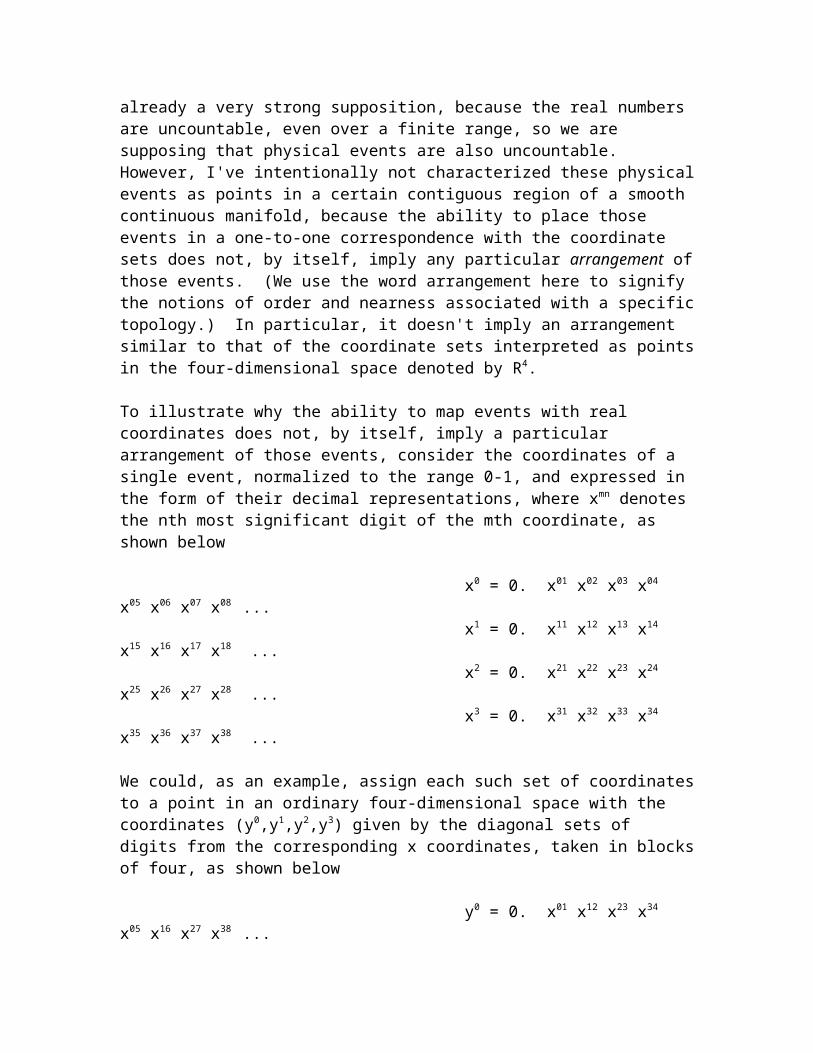
done. Einstein referred to allowing complex transformations, or non-symmetric, or increasing the number of dimensions, etc., but all these retain the continuum hypothesis. He doesn’t seem to have seriously considered relaxing this assumption, and allowing completely arbitrary transformations (unless this is what he had in mind when he referred to an “algebraic theory”). Ironically in his expositions of general relativity he often proudly explained that it gave an expression of physical laws valid for completely arbitrary transformations of the coordinates, but of course he meant arbitrary only up to diffeomorphism, which in the absolute sense is not very arbitrary at all. We mentioned in the previous section that diffeomorphically equivalent sets can be assigned the same topology, but from the standpoint of a physical theory it isn't self-evident which diffeomorphism is the right one (assuming there is one) for a particular set of physical entities, such as the events of spacetime.  Suppose we're able to establish a 1-to-1 correspondence between certain physical events and the sets of four real-valued numbers (x0,x1,x2,x3).  (As always, the superscripts are indices, not exponents.)  This is already a very strong supposition, because the real numbers are uncountable, even over a finite range, so we are supposing that physical events are also uncountable.  However, I've intentionally not characterized these physical events as points in a certain contiguous region of a smooth continuous manifold, because the ability to place those events in a one-to-one correspondence with the coordinate sets does not, by itself, imply any particular arrangement of those events.  (We use the word arrangement here to signify the notions of order and nearness associated with a specific topology.)  In particular, it doesn't imply an arrangement similar to that of the coordinate sets interpreted as points in the four-dimensional space denoted by R4.   To illustrate why the ability to map events with real coordinates does not, by itself, imply a particular arrangement of those events, consider the coordinates of a single event, normalized to the range 0-1, and expressed in the form of their decimal representations, where xmn denotes the nth most significant digit of the mth coordinate, as shown below                                     x0 = 0.  x01 x02 x03 x04   x05 x06 x07 x08

  ...                                    x1 = 0.  x11 x12 x13 x14   x15 x16 x17 x18  ...                                    x2 = 0.  x21 x22 x23 x24   x25 x26 x27 x28  ...                                    x3 = 0.  x31 x32 x33 x34   x35 x36 x37 x38  ... We could, as an example, assign each such set of coordinates to a point in an ordinary four-dimensional space with the coordinates (y0,y1,y2,y3) given by the diagonal sets of digits from the corresponding x coordinates, taken in blocks of four, as shown below                                     y0 = 0.  x01 x12 x23 x34   x05 x16 x27 x38

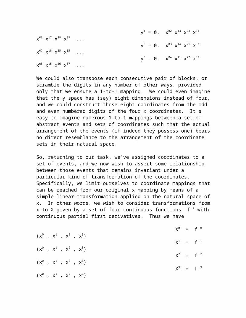
  ...                                    y1 = 0.  x02 x13 x24 x31   x06 x17 x28 x35  ...                                    y2 = 0.  x03 x14 x21 x32   x07 x18 x25 x35  ...                                    y3 = 0.  x04 x11 x22 x33   x08 x15 x26 x37  ... We could also transpose each consecutive pair of blocks, or scramble the digits in any number of other ways, provided only that we ensure a 1-to-1 mapping.  We could even

imagine that the y space has (say) eight dimensions instead of four, and we could construct those eight coordinates from the odd and even numbered digits of the four x coordinates.  It's easy to imagine numerous 1-to-1 mappings between a set of abstract events and sets of coordinates such that the actual arrangement of the events (if indeed they possess one) bears no direct resemblance to the arrangement of the coordinate sets in their natural space. So, returning to our task, we've assigned coordinates to a set of events, and we now wish to assert some relationship between those events that remains invariant under a particular kind of transformation of the coordinates.  Specifically, we limit ourselves to coordinate mappings that can be reached from our original x mapping by means of a simple linear transformation applied on the natural space of x.  In other words, we wish to consider transformations from x to X given by a set of four continuous functions  f i with continuous partial first derivatives.  Thus we have                                                 X0  =  f 0 (x0 , x1 , x2 , x3)                                                X1  =  f 1 (x0 , x1 , x2 , x3)                                                X2  =  f 2 (x0 , x1 , x2 , x3)                                                X3  =  f 3 (x0 , x1 , x2 , x3) Further, we require this transformation to posses a differentiable inverse, i.e., there exist differentiable functions Fi such that                                                 x0  =  F0 (X0 , X1 , X2 , X3)                                                x1  =  F1 (X0 , X1 , X2 , X3)                                                x2  =  F2 (X0 , X1 , X2 , X3)                                                x3  =  F3 (X0 , X1 , X2 , X3) A mapping of this kind is called a diffeomorphism, and two sets are said to be equivalent up to diffeomorphism if there is such a mapping from one to the other.  Any physical theory, such as general relativity, formulated in terms of tensor fields in spacetime automatically possess the freedom to choose the coordinate system from among a complete class of diffeomorphically equivalent systems.  From one point of view this can be seen as a tremendous generality and freedom from dependence on arbitrary coordinate systems.  However, as noted above, there are infinitely many systems of coordinates that are not diffeomorphically equivalent, so the limitation to equivalent systems up to diffeomorphism can also be seen as quite restrictive.   For example, no such functions can possibly reproduce the digit-scrambling transformations discussed previously, such as the mapping from x to y, because those mappings are everywhere discontinuous.  Thus we cannot get from x coordinates to y coordinates (or vice versa) by means of continuous transformations.  By restricting ourselves to differentiable transformations we're implicitly focusing our attention on one particular equivalence class of coordinate systems, with no a priori guarantee that this class of systems includes the most natural parameterization of physical events.  In fact,

we don't even know if physical events possess a natural parameterization, or if they do, whether it is unique. Recall that the special theory of relativity assumes the existence and identifiability of a preferred equivalence class of coordinate systems called the inertial systems.  The laws of physics, according to special relativity, should be the same when expressed with respect to any inertial system of coordinates, but not necessarily with respect to non-inertial systems of reference.  It was dissatisfaction with having given a preferred role to a particular class of coordinate systems that led Einstein to generalize the "gage freedom" of general relativity, by formulating physical laws in pure tensor form (general covariance) so that they apply to any system of coordinates from a much larger equivalence class, namely, those that are equivalent to an inertial coordinate system up to diffeomorphism.  This entails accelerated coordinate systems (over suitably restricted regions) that are outside the class of inertial systems.  Impressive though this achievement is, we should not forget that general relativity is still restricted to a preferred class of coordinate systems, which comprise only an infinitesimal fraction of all conceivable mappings of physical events, because it still excludes non-diffeomorphic transformations. It's interesting to consider how we arrive at (and agree upon) our preferred equivalence class of coordinate systems.  Even from the standpoint of special relativity the identification of an inertial coordinate system is far from trivial (even though it's often taken for granted).  When we proceed to the general theory we have a great deal more freedom, but we're still confined to a single topology, a single pattern of coherence.  How is this coherence apprehended by our senses?  Is it conceivable that a different set of senses might have led us to apprehend a different coherent structure in the physical world?  More to the point, would it be possible to formulate physical laws in such a way that they remain applicable under completely arbitrary transformations? 9.3  Higher-Order Metrics 

A similar path to the same goal could also be taken in those manifolds in which the line element is expressed in a less simple way, e.g., by a fourth root of a differential expression of the fourth degree…                                                                                                                Riemann, 1854

 Given three points A,B,C, let dx1 denote the distance between A and B, and let dx2 denote the distance between B and C. Can we express the distance ds between A and C in terms of dx1 and dx2? Since dx1, dx2, and ds all represent distances with comensurate units, it's clear that any formula relating them must be homogeneous in these quantities, i.e., they must appear to the same power. One possibility is to assume that ds is a linear combination of dx1 and dx2 as follows 

 

where g1 and g2 are constants. In a simple one-dimensional manifold this would indeed be the correct formula for ds, with  |g1| = |g2| = 1, except for the fact that it might give a negative sign for ds, contrary to the idea of an interval as a positive magnitude. To ensure the correct sign for ds, we might take the absolute value of the right hand side, which suggests that the fundamental equality actually involves the squares of the two sides of the above equation, i.e., the quantities ds, dx1, dx2 satisfy the relation 

 where we have put gij = gi gj. Thus we have g11g22   4(g12)2 = 0, which is the condition for factorability of the expanded form as the square of a linear expression. This will be the case in a one-dimensional manifold, but in more general circumstances we find that the values of the gij in the expanded form of (2) are such that the expression is not factorable into linear terms with real coefficients. In this way we arrive at the second-order metric form, which is the basis of Riemannian geometry. Of course, by allowing the second-order coefficients gij to be arbitrary, we make it possible for (ds)2 to be negative, analagous to the fact that ds in equation (1) could be negative, which is what prompted us to square both sides of (1), leading to equation (2). Now that (ds)2 can be negative, we're naturally led to consider the possibility that the fundamental relation is actually the equality of the squares of boths sides of (2). This gives 

 where the sum is evaluated for each ranging from 1 to n, where n is the dimension of the manifold. Once again, having arrived at this form, we immediately dispense with the assumption of factorability, and allow general fourth-order metrics. These are non-Riemannian metrics, although Riemann actually alluded to the possibility of fourth and higher order metrics in his famous inagural dissertation. He noted that 

The line element in this more general case would not be reducible to the square root of a quadratic sum of differential expressions, and therefore in the expression for the square of the line element the deviation from flatness would be an infinitely small quantity of degree two, whereas for the former manifolds [i.e., those whose squared line elements are sums of squares] it was an infinitely small quantity of degree four. This pecularity [i.e., this quantity of the second degree] in the latter manifolds therefore might well be called the planeness in the smallest parts…

 

It's clear even from his brief comments that he had given this possibility considerable thought, but he never published any extensive work on it. Finsler wrote a dissertation on this subject in 1918, so such metrics are now often called Finsler metrics. To visualize the effect of higher order metrics, recall that for a second-order metric the locus of points at a fixed distance ds from the origin must be a conic, i.e., an ellipse, hyperbola, or parabola. In contrast, a fourth-order metric allows more complicated loci of equi-distant points. When applied in the context of Minkowskian metrics, these higher-order forms raise some intriguing possibilities. For example, instead of a spacetime structure with a single light-like characteristic c, we could imagine a structure with two null characteristics, c1 and c2. Letting x and t denote the spacelike and timelike coordinates respectively, this means (ds/dt)4 vanishes for two values (up to sign) of dx/dt. Thus there are four roots given by c1 and c2, and we have 

The resulting metric is 

 The physical significance of this "metric" naturally depends on the physical meaning of the coordinates x and t. In Minkowski spacetime these represent what physical rulers and clocks measure, and we can translate these coordinates from one inertial system to another according to the Lorentz transformations while always preserving the form of the Minkowski metric with a fixed numerical value of c. The coordinates x and t are defined in such a way that c remains invariant, and this definition happily coincides with the physical measures of rulers and clocks. However, with two distinct light-like "eigenvalues", it's no longer possible for a single family of spacetime decompositions to preserve the values of both c1 and c2. Consequently, the metric will take the form of (3) only with respect to one particular system of xt coordinates. In any other frame of reference at least one of c1 and c2 must be different. Suppose that with respect to a particular inertial system of coordinates x,t the spacetime metric is given by (3) with c1 = 1 and c2 = 2. We might also suppose that c1 corresponds to the null surfaces of electromagnetic wave propagation, just as in Minkowski spacetime. Now, with respect to any other system of coordinates x',t' moving with speed v relative to the x,t coordinates, we can decompose the absolute intervals into space and time components such that c1 = 1, but then the values of the other lightlines (corresponding to c2') must be (v + c2)/(1 + v c2) and (v c2)/(1 v c2). Consequently, for states of motion far from the one in which the metric takes the special form (3), the

metric will become progressively more asymmetrical. This is illustrated in the figure below, which shows contours of constant magnitude of the squared interval. 

 Clearly this metric does not correspond to the observed spacetime structure, even in the symmetrical case with v = 0, because it is not Lorentz-invariant. As an alternative to this structure containing "super-light" null surfaces we might consider metrics with some finite number of "sub-light" null surfaces, but the failure to exhibit even approximate Lorentz-invariance would remain. However, it is possible to construct infinite-order metrics with infinitely many super-light and/or sub-light null surfaces, and in so doing recover a structure that in many respect is virtually identical to Minkowski spacetime, except for a set (of spacetime trajectories) of measure zero. This can be done by generalizing (3) to include infinitely many discrete factors 

 where the values of ci represent an infinite family of sub-light parameters given by 

 A plot showing how this spacetime structure develops as n increases is shown below.  

 This illustrates how, as the number of sub-light cones goes to infinity, the structure of the manifold goes over to the usual Minkowski pseudometric, except for the discrete null sub-light surfaces which are distributed throughout the interior of the future and past light cones, and which accumulate on the light cones. The sub-light null surfaces become so thin that they no linger show up on these contour plots for large n, but they remain present to all orders. In the limit as n approaches infinity they become discrete null trajectories embedded in what amounts to ordinary Minkowski spacetime. To see this, notice that if none of the factors on the right hand side of (4) is exactly zero we can take the natural log of both sides to give 

 Thus the natural log of (ds)2 is the asymptotic average of the natural logs of the quantities (dx)2ci

2(dt)2. Since the values of ci accumultate on 1, it's clear that this converges on the usual Minkowski metric (provided we are not precisely on any of the discrete sub-light null surfaces). 

The preceding metric was based purely on sub-light null surfaces. We could also include n super-light null surfaces along with the n sub-light null surfaces, yielding an asymptotic family of metrics which, again, goes over to the usual Minkowski metric as n goes to infinity (except for the discrete null surface structure). This metric is given by the formula 

 where the values of ci are generated as before. The results for various values of n are illustrated in the figure below.  

 Notice that the quasi Lorentz-invariance of this metric has a subtle periodicity, because any one of the sublight null surfaces can be aligned with the time axis by a suitable choice of velocity, or the time axis can be placed "in between" two null surfaces. In a 1+1 dimensional spacetime the structure is perfectly symmetrical modulo this cycle from one null surface to the next. In other words, the set of exactly equivalent reference systems corresponds to a cycle with a period of , which is the increment between each ci and ci+1. However, with more spatial dimensions the sub-light null structure is subtly less symmetrical, because each null surface represents a discrete cone, which associates two of the trajectories in the xt plane as the sides of a single cone. Thus there must be an absolutely innermost cone, in the topological sense, even though that cone may be far off

center, i.e., far from the selected time axis. Similarly for the super-light cones (or spheres), there would be a single state of motion with respect to which all of those null surfaces would be spherically symmetrical. Only the accumulation shell, i.e., the actual light-cone itself, would be spherically symmetrical with respect to all states of motion. 9.4  Polarization and Spin 

Every ray of light has therefore two opposite sides… And since the crystal by this disposition or virtue does not act upon the rays except when one of their sides of unusual refraction looks toward that coast, this argues a virtue or disposition in those sides of the rays which answers to and sympathizes with that virtue or disposition of the crystal, as the poles of two magnets answer to one another…                                                                                                                Newton, 1717

 A transparent crystalline substance, now known as calcite, was discovered by a naval expedition to Iceland in 1668, and samples of this “Iceland crystal” were examined by the Danish scientist Erasmus Bartholin, who noticed that a double image appeared when objects were viewed through this crystal. He found that rays of light passing through calcite are split into two refracted rays. Some of the incoming light is always refracted at the normal angle of refraction for the density of the substance and a given angle of incidence, but some of the incoming light is refracted at a different angle. If the incident ray is perpendicular to the face of the crystal, the ordinary ray undergoes no refraction and passes straight through, just as we would expect, but the extraordinary ray is refracted upon entering the crystal and again upon departing the crystal. Bartholin noted that the direction in which the extraordinary ray diverges from the perpendicular as it passes into the crystal depends on the orientation of the crystal about the incident axis. Thus by rotating the crystal about the incident axis, the second image appearing through the crystal revolves around the first image. This phenomenon could have been observed at any time in human history, and might not have been regarded as terribly significant, but by the middle of the 17th century the study of optics had reached a point where the occurrence of two distinct refracted rays was a clear anomaly. Bartholin called this “one of the greatest wonders that nature has produced”. (It’s interesting that Bartholin’s daughter, Anne Marie, married Ole Roemer, whose discovery of the finite speed of light was discussed in Section 3.3.) Christiaan Huygens had previously derived the ordinary law of refraction from his wave theory light by assuming that the speed of light in a refracting substance is the same in all directions, i.e., isotropic. When Huygens learned of the double refraction in the Iceland crystal (also known as Iceland spar) he concluded that the crystal must contain two different media interspersed, and that the speed of light is isotropic in one of these media but anisotropic in the other. Hence he imagined that two distinct wave fronts emanated from each point, one spherical and the other ellipsoidal, and the directions of the two rays were normal to these two wave fronts. He didn’t explain why part of the light propagated purely in one of the media, and part of the light purely in the other. Moreover, he

discovered another very remarkable phenomena related to this double refraction that was even more difficult to reconcile with his implicitly longitudinal conception of light waves. He found that if a ray of light, after passing through an Iceland crystal, is passed through a second crystal aligned parallel with the first, then all of the ordinary ray passes through the second crystal without refraction, and all of the extraordinary ray is refracted in the second crystal just as it was in the first. On the other hand, if the secondary crystals are aligned perpendicular to the first, the refracted ray from the first crystal is not refracted at all in the second crystal, whereas the unrefracted ray from the first crystal undergoes refraction in the second. These two cases are depicted in the figures below.  

 Huygens was unable to account for this behavior in any way that was consistent with his conception of light as a longitudinal wave with radial symmetry. He conceded 

…it seems that one is obliged to conclude that the waves of light, after having passed through the first crystal, acquire a certain form or disposition in virtue of which, when meeting the texture of the second crystal, in certain positions, they can move the two different kinds of matter which serve for the two species of refraction; and when meeting the second crystal in another position are able to move only one of these kinds of matter. But to tell how this occurs, I have hitherto found nothing which satisfies me.

 Newton considered this phenomena to be inexplicable “if light be nothing other than pression or motion through an aether”, and argued that “the unusual refraction is [due to] an original property of the rays”, namely, an axial asymmetry or sidedness, which he thought must be regarded as an intrinsic property of individual corpuscles of light. At the beginning of the 19th century the “sidedness” of Newton of reconciled with the wave concept of Huygens by the idea of light as a transverse (rather than longitudinal) wave. Later this transverse wave was found to be a feature of the electromagnetic waves predicted by Maxwell’s equations, according to which the electric and magnetic fields oscillate transversely in the plane normal to the direction of motion (and perpendicular to each other). Thus an electromagnetic wave "looks" something like this: 

 where E signifies the oscillating electric field and B the magnetic field. The wave is said to be polarized in the direction of E. The osculating planes are perpendicular to each other, but their orientations are not necessarily fixed - it's possible for them to rotate like a windmill about the axis of propagation. In general the electric field of a plane wave of frequency propagating along the z axis of Cartesian coordinates can be resolved into two perpendicular components that can be written as 

 where is the phase difference between the two components, and Cx and Cy are the constant amplitudes. If the amplitudes of these two components both equal a single constant E0, and if the phase difference is –/2, then remembering the trigonometric identity sin(u) = cos(u /2), we have 

 In this case the amplitude of the overall wave is constant, and, as can be seen in the figure below, the electric field vector at constant z rotates (at the angular speed ) in the clockwise direction as seen by an observer looking back toward the approaching wave. 

 

This is conventionally called right-circularly polarized light. On the other hand, if the amplitudes are equal but the phase difference is +/2, then remembering the trigonometric identity sin(u) = cos(u + p/2), the two components are 

 so the direction of the electric field rotates in the counter-clockwise direction. This is called left-circularly polarized light. If we superimpose left and right circularly polarized waves (with the same frequency and phase), The result is simply 

 which represents a linearly polarized wave, since the electric field oscillates entirely in the xz plane. By combining left and right circularly polarized light in other proportions and with other phase relations, we can also produce what are called elliptically polarized light waves, which are intermediate between the extremes of circularly polarized and linearly polarized light. Conversely, a circularly polarized light wave can be produced by combining two perpendicular linearly polarized waves. A typical plane wave of ordinary light (such as from the Sun) consists of components with all possible polarizations mixed together, but it can be decomposed into left and right circularly polarized waves, and this can be done relative to any orthogonal set of axes. Calcite crystals (as well as some other substances) have an isotropic index of refraction for light whose electric field oscillates in one particular plane, but an anisotropic index of refraction for light whose electric field oscillates in the perpendicular plane. Hence it acts as a filter, decomposing the incident wave (normal to the surface) into perpendicular linearly polarized waves aligned with the characteristic axis of the crystal. As the wave enters the crystal, only the component whose electric plane of oscillation encounters anisotropic refractivity is subjected to refraction. This is the classical account of the phenomena observed by Bartholin and Huygens. It could be argued that the classical account of polarization phenomena is incomplete, because it relies on the assumption that a superposition of plane waves can be decomposed into an arbitrary set of orthogonal components, and that the interactions of those components with matter will yield the same results, regardless of the chosen basis of decomposition. The difficulty can be seen by considering how a polarizing crystal prevents exactly half of the waves from passing straight through while allowing other half to pass. The incident beam consists of waves whose polarization axes are distributed uniformly in all direction, so one might expect to find that only a very small fraction of the waves would pass through a perfect polarizing substance. In fact, the fraction of waves from a uniform distribution with polarizations exactly aligned with the polarizing axis of a substance should be vanishingly small. Likewise it isn’t easy to explain, from the standpoint of classical electrodynamics, why half of the incident wave energy is diverted in one discrete direction, rather than being distributed over a range of refraction angles. The process seems to be discretely binary, i.e., each bit of incident energy must go in one of just two directions, even though the polarization angles of the incident

energy are uniformly distributed over all directions. The precise mechanism for how this comes about requires a detailed understanding of the interactions between matter and electromagnetic radiation – something which classical electrodynamics was never able to provide. If we discard the extraordinary ray emerging from a calcite polarizing prism, the crystal functions as a filter, producing a beam of a linearly polarized light. The thickness of a polarizing filter isn't crucial (assuming the polarization axis is perfectly uniform throughout the substance), because the first surface effectively "selects" the suitably aligned waves, which then pass freely through the rest of the substance. The light emerging from the other side is plane-polarized with half the intensity of the incident light. Now, as noted above, if we pass this polarized beam through another polarizing filter oriented parallel to the first, then all the energy of the incident polarized beam will be passed through the second filter. On the other hand, if the second filter is oriented perpendicular to the first, none of the polarized beams energy will get through the second filter. For intermediate angles, Etienne Malus (a captain in the army of Napoleon Bonaparte) discovered in 1809 that the intensity of the beam emerging from the second polarizing filter is  I cos()2,  where I is the intensity of the beam emerging from the first filter and is the angle between the two filters. Incidentally, it’s possible to convert circularly polarized incident light into plane-polarized light of the same intensity. The traditional method is to use a "quarter-wave plate" thickness of a crystal substance such as mica. In this case we're not masking the non-aligned components, but rather introducing a relative phase shift between them so as to force them into alignment. Of course, a particular thickness of plate only "works" this way for a particular frequency. In 1922 the Dutch physicists Otto Stern and Walther Gerlach made a discovery remarkably similar to that of Erasmus Bartholin, but instead of light rays their discovery involved the trajectories of elementary particles of matter. They passed a beam of particles (atoms of silver) through an oriented magnetic field, and found that the beam split into two beams, with about half the particles in each beam, one deflected up (relative to the direction of the magnetic field) and the other down. This is depicted in the figure below. 

 Ultimately this behavior was recognized as being a consequence of the intrinsic spin of elementary particles. The idea of intrinsic spin was introduced by Uhlenbech and Goudsmit in 1925, and was soon incorporated (albeit in a somewhat ad hoc way) into the formalism of quantum mechanics by postulating that the wave function of a particle can

be decomposed into two components, which we might label UP and DOWN, relative to any given orientation of the magnetic field. These components are weighted and the sum of the squares of the weights equals 1. (Of course, the overall state-vector for the particle can be expressed as the Cartesian product of a non-spin vector times the spin vector.) The observable "spin" then corresponds to three operators that are proportional to the Pauli spin matrices: 

 These operators satisfy the commutation relations 

 as we would expect by the correspondence principle from ordinary (classical) angular momentum. Not surprisingly, this non-commutation is closely related to the non-commutation of ordinary spatial rotations of a classical particle, in the sense that they're both related to the cross-product of orthogonal vectors. Given an orthogonal coordinate system [x,y,z] the angular momentum of a classical particle with momentum [px, py, pz] is (in component form) 

 Guided by the correspondence principle, we replace the classical components px, py, pz with their quantum mechanical equivalents, the differential operators 

, leading to the S operators noted above. Although this works, it is not entirely satisfactory, first because it is ad hoc, and second because it is not relativistic. Both of these shortcomings were eliminated by Dirac in 1928 when he developed the first relativistic equation for an elementary massive particle. The Dirac equation is one of the greatest examples of the heuristic power of the principle of relativity, leading not only to an understanding of the necessity of intrinsic spin, but also to the prediction of anti-matter, and ultimately to quantum field theory. Recall from Section 2.3 that the invariant spacetime interval along the path of a timelike particle of mass m in special relativity is 

 and if we multiply through by m2/(dt)2 and make the identifications E = m(dt/d), px = m(dx/d), etc., this gives 

 Also, if we postulate that the particle is described by a wave function (t,x,y,z) we can differentiate with respect to to give 

 multiplying through by m and making the identifications for E, px, py, pz, we get 

 This relation would be equivalent to equation (1) if we put 

 where  is a constant. This suggests the operator correspondences 

 on the basis of which equation (2) can be re-written as 

 which, if we identify  with the reduced Planck constant h/(2), is the Klein-Gordon wave equation. Unfortunately the solutions of this equation do not give positive-definite probabilities, so it was ruled out as a possible quantum mechanical wave function for a massive particle. Schrödinger’s provisional alternative was to base his wave mechanics on the non-relativistic version of equation (1), which is simply E = p2/(2m). This led to the familiar Schrödinger equation, whose solutions do give positive-definite probabilities, and which was highly successful in non-relativistic contexts. Still, Dirac was dissatisfied, and sought a relativistic wave equation with positive-definite probabilities. Dirac’s solution was to factor the quadratic equation (1) into linear factors, and take one of those factors as the basis of the quantum mechanical wave equation. Of course, equation (1) doesn’t factor if we restrict ourselves to the set of real numbers, but it can be factored in different classes of mathematical entities, just as x2+1 can’t be factored if we are restricted to real numbers, but it factors as (x+i)(xi) if we allow imaginary as well as real units. 

In order to factor equation (1), Dirac postulated a set of basis variables 0, 1, 2, and 3 (not necessarily commuting) such that 

 Expanding the product and collecting terms, we find that this is a valid equality if and only if the four variables j satisfy the relations 

 for all i,j = 0,1,2,3 with i ≠ j. These four quantities, along with unity, form the basis of what is called a Clifford algebra. The natural representation of these “quantities” is as 4x4 matrices. Equation (1) is solved provided either of the factors equals zero. Setting the first factor equal to zero and making the operator substitutions for energy and momentum, we arrive at Dirac’s equation 

 Since the operator is four-dimensional, the wave function must be a vector with four components, i.e., we have 

 The four components encode the different possible intrinsic spin states of the particle, subsuming the earlier ad hoc two-dimensional state vector. The appearance of four components instead of just two is due to the fact that these state vectors also encompass negative energy states as well as positive energy states. This was inevitable, considering that the relativistic equation (1) is satisfied equally well by –E as well as +E. It may be surprising at first that equation (4), which is linear, is nevertheless covariant under Lorentz transformations. The covariance certainly isn’t obvious, and it is achieved only by stipulating that the components of transform not as an ordinary four-vector, but as two spinors. Thus the requirement for Lorentz covariance leads directly to the existence of intrinsic spin for any massive particle described by Dirac’s equation, including electrons. (Such particles are said to possess “spin 1/2”, since it can be shown that the angular momentum represented by their intrinsic spin is .) In addition, when the interaction with an electromagnetic field is included in the Dirac equation, the requirement for Lorentz covariance leads to the existence of anti-particles. The positron,

which is the anti-particle of the electron, was predicted by Dirac around 1929, and found experimentally just two years later. Fundamentally, the Dirac equation introduced, for the first time, the idea that any relativistic treatment of one particle must inevitably involve consideration of other particles, and from this emerged the concept of second quantization and quantum field theory. In effect, quantum field theory requires us to consider not just the field of a single identified particle, but the field of all such fields. (It’s interesting to compare this with the view of the metric of spacetime as the “field of all fields” discussed in Section 4.6.) One outcome of quantum field theory was a quantization of the electromagnetic field, the necessity of which had been pointed out by Einstein as early as 1905. On an elementary level, Maxwell’s equations are inadequate to describe the phenomena of radiation. The quantum of electromagnetic radiation is called the photon, which behaves in some ways like an elementary particle, although it is massless, and therefore always propagates at the speed of light. Hence the "spin axis" of a photon is always parallel to its direction of motion, pointing either forward or backward, as illustrated below. 

 These two states correspond to left-handed and right-handed photons. Whenever a photon is absorbed by an object, an angular momentum of either  or  is imparted to the object. Each photon is characterized not only by its energy (frequency) and its phase, but also by it’s propensity to exhibit each of the two possible states of spin when it interacts with an object. A beam of light, consisting of a large number of photons, is characterized by the energies, phase relations, and spin propensities of its constituent photons. This could be said to vindicate Newton’s belief that rays of light posses a previously unknown “original property” that affects how they are refracted. Recall that, in classical electromagnetic theory, the plane of oscillation of the electric field of circularly polarized light rotates about the axis of propagation (in one direction or the other). When such light impinges on a surface, it imparts angular momentum due to the rotation of the electric field. In quantum theory this corresponds to a stream of photons with a high propensity for being right-handed (or for being left-handed), so that each photon contributes to the overall angular momentum imparted to the absorbing object. On the other hand, linearly polarized light (in classical electrodynamics) does not impart any angular momentum to the absorbing object. This is represented in quantum theory by a stream of photons, each with equal propensity to exhibit right-handed or left-handed spin. Each individual interaction, i.e., each absorption of a photon, imparts either  or

 to the absorbing object, so if the intensity of a linearly polarized beam of light is lowered to the point that only one photon is transmitted at a time, it will appear to be circularly polarized (either left or right) for each photon, which of course is not predicted by classical theory. (In a sense, Maxwell’s equations can be regarded as a crude form of the Schrödinger equation for light, but it obviously does not represent all the quantum mechanical effects.) However, for a large stream of such photons, the net angular

momentum is essentially zero, because half of the photons interact in the right-handed sense and half in the left-handed sense. This corresponds (loosely) to the fact in classical theory that linearly polarized light can be regarded as a superposition of left and right circularly polarized light. Incidentally, most people have personal "hands on" knowledge of polarized electromagnetic waves without even realizing it. The waves broadcast by a radio or television tower are naturally polarized, and if you've ever adjusted the orientation of "rabbit ears" and found that your reception is better at some orientations than at others, for a particular station, you've demonstrated the effects of electromagnetic wave polarization. The behavior of intrinsic spin of elementary particles can be used to illustrate some important features of quantum mechanics – features which Einstein famously referred to as “spooky action at a distance”. This behavior is discussed in the next section. 9.5  Entangled Events 

Anyone who is not shocked by quantum theory has not understood it.                                                                                Niels Bohr, 1927

 A paper written by Einstein, Podalsky, and Rosen (EPR) in 1935 described a thought experiment which, the authors believed, demonstrated that quantum mechanics does not provide a complete description of physical reality, at least not if we accept certain common notions of locality and realism. Subsequently the EPR experiment was refined by David Bohm (so it is now called the EPRB experiment) and analyzed in detail by John Bell, who highlighted a fascinating subtlety that Einstein, et al, may have missed. Bell showed that the outcomes of the EPRB experiment predicted by quantum mechanics are inherently incompatible with conventional notions of locality and realism combined with a certain set of assumptions about causality. The precise nature of these causality assumptions is rather subtle, and Bell found it necessary to revise and clarify his premises from one paper to the next. In Section 9.6 we discuss Bell's assumptions in detail, but for the moment we'll focus on the EPRB experiment itself, and the outcomes predicted by quantum mechanics. Most actual EPRB experiments are conducted with photons, but in principle the experiment could be performed with massive particles. The essential features of the experiment are independent of the kind of particle we use. For simplicity we'll describe a hypothetical experiment using electrons (although in practice it may not be feasible to actually perform the necessary measurements on individual electrons). Consider the decay of a spin-0 particle resulting in two spin-1/2 particles, an electron and a positron, ejected in opposite directions. If spin measurements are then performed on the two individual particles, the correlation between the two results is found to depend on the difference between the two measurement angles. This situation is illustrated below, with and signifying the respective measurement angles at detectors 1 and 2. 

 Needless to say, the mere existence of a correlation between the measurements on these two particles is not at all surprising. In fact, this would be expected in most classical models, as would a variation in the correlation as a function of the absolute difference = | | between the two measurement angles. The essential strangeness of the quantum mechanical prediction is not the mere existence of a correlation that varies with , it is the non-linearity of the predicted variation.  If the correlation varied linearly as ranged from 0 to , it would be easy to explain in classical terms. We could simply imagine that the decay of the original spin-0 particle produced a pair of particles with spin vectors pointing oppositely along some randomly chosen axis. Then we could imagine that a measurement taken at any particular angle gives the result UP if the angle is within /2 of the positive spin axis, and gives the result DOWN otherwise. This situation is illustrated below: 

 Since the spin axis is random, each measurement will have an equal probability of being UP or DOWN. In addition, if the measurements on the two particles are taken in exactly the same direction, they will always give opposite results (UP/DOWN or DOWN/UP), and if they are taken in the exact opposite directions they will always give equal results (UP/UP or DOWN/DOWN). Also, if they are taken at right angles to each other the results will be completely uncorrelated, meaning they are equally likely to agree or disagree. In general, if denotes the absolute value of the angle between the two spin measurements, the above model implies that the correlation between these two measurements would be C(q) = (2/) 1, as plotted below. 

 This linear correlation function is consistent with quantum mechanics (and confirmed by experiment) if the two measurement angles differ by = 0, /2, or , giving the correlations 1, 0, and +1 respectively.  However, for intermediate angles, quantum theory predicts (and experiments confirm) that the actual correlation function for spin-1/2 particles is not the linear function shown above, but the non-linear function given by C() = cos(), as shown below 

On this basis, the probabilities of the four possible joint outcomes of spin measurements performed at angles differing by are as shown in the table below. (The same table would apply to spin-1 particles such as photons if we replace with 2.)   

 To understand why the shape of this correlation function defies explanation within the classical framework of local realism, suppose we confine ourselves to spin measurements

along one of just three axes, at 0, 120, and 240 degrees. For convenience we will denote these axes by the symbols A, B, and C respectively. Several pairs of particles are produced and sent off to two distant locations in opposite directions. In both locations a spin measurement along one of the three allowable axes is performed, and the results are recorded. Our choices of measurements (A, B, or C) may be arbitrary, e.g., by flipping coins, or by any other means. In each location it is found that, regardless of which measurement is made, there is an equal probability of spin UP or spin DOWN, which we will denote by "1" and "0" respectively. This is all that the experimenters at either site can determine separately.  However, when all the results are brought together and compared in matched pairs, we find the following joint correlations 

 The numbers in this matrix indicate the fraction of times that the results agreed (both 0 or both 1) when the indicated measurements were made on the two members of a matched pair of objects. Notice that if the two distant experimenters happened to have chosen to make the same measurement for a given pair of particles, the results never agreed, i.e., they were always the opposite (1 and 0, or 0 and 1). Also notice that, if both measurements are selected at random, the overall probability of agreement is 1/2. The remarkable fact is that there is no way (within the traditional view of physical processes) to prepare the pairs of particles in advance of the measurements such that they will give the joint probabilities listed above. To see why, notice that each particle must be ready to respond to any one of the three measurements, and if it happens to be the same measurement as is selected on its matched partner, then it must give the opposite answer. Hence if the particle at one location will answer "0" for measurement A, then the particle at the other location must be prepared to give the answer "1" for measurement A. There are similar constraints on the preparations for measurements B and C, so there are really only eight ways of preparing a pair of particles 

These preparations - and only these - will yield the required anti-correlation when the same measurement is applied to both objects. Therefore, assuming the particles are pre-programmed (at the moment when they separate from each other) to give the appropriate result for any one of the nine possible joint measurements that might be performed on them, it follows that each pair of particles must be pre-programmed in one of the eight ways shown above. It only remains now to determine the probabilities of these eight preparations. The simplest state of affairs would be for each of the eight possible preparations to be equally probable, but this yields the measurement correlations shown below 

 Not only do the individual joint probabilities differ from the quantum mechanical predictions, this distribution gives an overall probability of agreement of 1/3, rather than 1/2 (as quantum mechanics says it must be), so clearly the eight possible preparations cannot be equally likely. Now, we might think some other weighting of these eight preparation states will give the right overall results, but in fact no such weighting is possible. The overall preparation process must yield some linear convex combination of the eight mutually exclusive cases, i.e., each of the eight possible preparations must have some fixed long-term probability, which we will denote by a, b,.., h, respectively. These probabilities are all positive values in the range 0 to 1, and the sum of these eight values is identically 1. It follows that the sum of the six probabilities b through g must be less than or equal to 1. This is a simple form of "Bell's inequality", which must be satisfied by any local realistic model of the sort that Bell had in mind. However, the joint probabilities in the correlation table predicted by quantum mechanics imply 

 Adding these three expressions together gives 2(b + c + d + e + f + g) = 9/4, so the sum of the probabilities b through g is 9/8, which exceeds 1. Hence the results of the EPRB experiment predicted by quantum mechanics (and empirically confirmed) violate Bell's inequality. This shows that there does not exist a linear combination of those eight preparations that can yield the joint probabilities predicted by quantum mechanics, so there is no way of accounting for the actual experimental results by means of any realistic local physical model of the sort that Bell had in mind. The observed violations of Bell's inequality in EPRB experiments imply that Bell's conception of local realism is inadequate to represent the actual processes of nature. The causality assumptions underlying Bell's analysis are inherently problematic (see Section 9.7), but the analysis is still important, because it highlights the fundamental inconsistency between the predictions of quantum mechanics and certain conventional ideas about causality and local realism. In order to maintain those conventional ideas, we would be forced to conclude that information about the choice of measurement basis at one detector is somehow conveyed to the other detector, influencing the outcome at that detector, even though the measurement events are space-like separated. For this reason, some people have been tempted to think that violations of Bell's inequality imply superluminal communication, contradicting the principles of special relativity. However, there is actually no effective transfer of information from one measurement to the other in an EPRB experiment, so the principles of special relativity are safe. One of the most intriguing aspects of Bell's analysis is that it shows how the workings of quantum mechanics (and, evidently, nature) involve correlations between space-like separated events that seemingly could only be explained by the presence of information from distant locations, even though the separate events themselves give no way of inferring that information. In the abstract, this is similar to "zero-information proofs" in mathematics.  To illustrate, consider a "twins paradox" involving a pair of twin brothers who are separated and sent off to distant locations in opposite directions. When twin #1 reaches his destination he asks a stranger there to choose a number x1 from 1 to 10, and the twin writes this number down on a slip of paper along with another number y1 of his own choosing. Likewise twin #2 asks someone at his destination to choose a number x2, and he writes this number down along with a number y2 of his own choosing. When the twins are re-united, we compare their slips of paper and find that |y2 y1| = (x2 x1)2. This is really astonishing. Of course, if the correlation was some linear relationship of the form y2 y1 = A(x2 x1) + B for any pre-established constants A and B, the result would be quite easy to explain. We would simply surmise that the twins had agreed in advance that twin #1 would write down y1 = Ax1 B/2, and twin #2 would write down y2 = Ax2 + B/2. However, no such explanation is possible for the observed non-linear relationship, because there do not exist functions f1 and f2 such that f2(x2) f1(x1) = (x2 x1)2. Thus if we assume the numbers x1 and x2 are independently and freely selected, and there is no communication between the twins after they are separated, then there is no "locally realistic" way of accounting for this non-linear correlation. It seems as though one or both of the twins must have had knowledge of his brother's numbers when writing down his

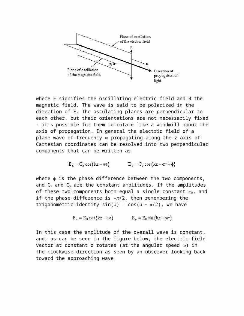
own number, despite the fact that it is not possible to infer anything about the individual values of x2 and y2 from the values of x1 and y1 or vice versa. In the same way, the results of EPRB experiments imply a greater degree of inter-dependence between separate events than can be accounted for by traditional models of causality. One possible idea for adjusting our conceptual models to accommodate this aspect of quantum phenomena would be to deny the existence of any correlations until they becomes observable. According to the most radical form of this proposal, the universe is naturally partitioned into causally compact cells, and only when these cells interact do their respective measurement bases become reconciled, in such a way as to yield the quantum mechanical correlations. This is an appealing idea in many ways, but it's far from clear how it could be turned into a realistic model. Another possibility is that the preparation of the two particles at the emitter and the choices of measurement bases at the detectors may be mutually influenced by some common antecedent event(s). This can never be ruled out, as discussed in Section 9.6. Lastly, we mention the possibility that the preparation of the two particles may be conditioned by the measurements to which they are subjected. This is discussed in Section 9.10. 

9.6  Von Neumann's Postulate and Bell’s Freedom 

If I have freedom in my love,And in my soul am free,Angels alone, that soar above,Enjoy such liberty.            Richard Lovelace, 1649

 In quantum mechanics the condition of a physical system is represented by a state vector, which encodes the probabilities of each possible result of whatever measurements we may perform on the system. Since the probabilities are usually neither 0 nor 1, it follows that for a given system with a specific state vector, the results of measurements generally are not uniquely determined. Instead, there is a set (or range) of possible results, each with a specific probability. Furthermore, according to the conventional interpretation of quantum mechanics (the so-called Copenhagen Interpretation of Niels Bohr, et al), the state vector is the most complete possible description of the system, which implies that nature is fundamentally probabilistic (i.e., non-deterministic). However, some physicists have questioned whether this interpretation is correct, and whether there might be some more complete description of a system, such that a fully specified system would respond deterministically to any measurement we might perform. Such proposals are called 'hidden variable' theories.  In his assessment of hidden variable theories in 1932, John von Neumann pointed out a set of five assumptions which, if we accept them, imply that no hidden variable theory can possibly give deterministic results for all measurements. The first four of these assumptions are fairly unobjectionable, but the fifth seems much more arbitrary, and has been the subject of much discussion. (The parallel with Euclid's postulates, including the controversial fifth postulate discussed in Chapter 3.1, is striking.) To understand von

Neumann's fifth postulate, notice that although the conventional interpretation does not uniquely determine the outcome of a particular measurement for a given state, it does predict a unique 'expected value' for that measurement. Let's say a measurement of X on a system with a state vector has an expected value denoted by <X;>, computed by simply adding up all the possible results multiplied by their respective probabilities. Not surprisingly, the expected values of observables are additive, in the sense that 

 In practice we can't generally perform a measurement of X+Y without disturbing the measurements of X and Y, so we can't measure all three observables on the same system. However, if we prepare a set of systems, all with the same initial state vector , and perform measurements of X+Y on some of them, and measurements of X or Y on the others, then the averages of the measured values of X, Y, and X+Y (over sufficiently many systems) will be related in accord with (1). Remember that according to the conventional interpretation the state vector is the most complete possible description of the system. On the other hand, in a hidden variable theory the premise is that there are additional variables, and if we specify both the state vector AND the "hidden vector" H, the result of measuring X on the system is uniquely determined. In other words, if we let <X;,H> denote the expected value of a measurement of X on a system in the state (,H), then the claim of the hidden variable theorist is that the variance of individual measured values around this expected value is zero. Now we come to von Neumann's controversial fifth postulate. He assumed that, for any hidden variable theory, just as in the conventional interpretation, the averages of X+Y, X and Y evaluated over a set of identical systems are additive. (Compare this with Galileo's assumption of simple additivity for the composition of incommensurate speeds.) Symbolically, this is expressed as 

 for any two observables X and Y. On this basis he proved that the variance ("dispersion") of at least one observable's measurements must be greater than zero. (Technically, he showed that there must be an observable X such that <X2> is not equal to <X>2.) Thus, no hidden variable theory can uniquely determine the results of all possible measurements, and we are compelled to accept that nature is fundamentally non-deterministic. However, this is all based on (2), the assumption of additivity for the expectations of identically prepared systems, so it's important to understand exactly what this assumption means. Clearly the words "identically prepared" mean something different under the conventional interpretation than they do in the context of a hidden variable theory. Conventionally, two systems are said to be identically prepared if they have the same

state vector (), but in a hidden variable theory two states with the same state vector are not necessarily "identical", because they may have different hidden vectors (H). Of course, a successful hidden variable theory must satisfy (1) (which has been experimentally verified), but must it necessarily satisfy (2)? Relation (1) implies that the averages of <X;,H>, etc, evaluated over all applicable hidden vectors H, leads to (1), but does it necessarily follow that (2) is satisfied for every (or even for ANY) specific value of H? To give a simple illustration, consider the following trivial set of data: 

 The averages over these four "conventionally indistinguishable" systems are <X;3> = 3, <Y;3> = 4, and <X+Y;3> = 7, so relation (1) holds. However, if we examine the "identically prepared" systems taking into account the hidden components of the state, we really have two different states (those with H=1 and those with H=2), and we find that the results are not additive (but they are deterministic) in these fully-defined states. Thus, equation (1) clearly doesn't imply equation (2). (If it did, von Neumann could have said so, rather than taking it as an axiom.) Of course, if our hidden variable theory is always going to satisfy (1), we must have some constraints on the values of H that arise among "conventionally indistinguishable" systems. For example, in the above table if we happened to get a sequence of systems all in the same condition as System #1 we would always get the results X=2, Y=5, X+Y=5, which would violate (1). So, if (2) doesn't hold, then at the very least we need our theory to ensure a distribution of the hidden variables H that will make the average results over a set of "conventionally indistinguishable" systems satisfy relation (1). (In the simple illustration above, we would just need to ensure that the hidden variables are equally distributed between H=1 and H=2.) In Bohm's 1952 theory the hidden variables consist of precise initial positions for the particles in the system – more precise than the uncertainty relations would typically allow us to determine - and the distribution of those variables within the uncertainty limits is governed as a function of the conventional state vector, . It's also worth noting that, in order to make the theory work, it was necessary for to be related to the values of H for separate particles instantaneously in an explicitly non-local way. Thus, Bohm's theory is a counter-example to von Neumann's theorem, but not to Bell's (see below). Incidentally, it may be worth noting that if a hidden variable theory is valid, and the variance of all measurements around their expectations are zero, then the terms of (2) are not only the expectations, they are the unique results of measurements for a given and H. This implies that they are eigenvalues, of the respective operators, whereas the

expectations for those operators are generally not equal to any of the eigenvalues. Thus, as Bell remarked, "[von Neumann's] 'very general and plausible postulate' is absurd". Still, Gleason showed that we can carry through von Neumann's proof even on the weaker assumption that (2) applies to commuting variables. This weakened assumption has the advantage of not being self-evidently false. However, careful examination of Gleason's proof reveals that the non-zero variances again arise only because of the existence of non-commuting observables, but this time in a "contextual" sense that may not be obvious at first glance. To illustrate, consider three observables X,Y,Z. If X and Y commute and X and Z commute, it doesn't follow that Y and Z commute. We may be able to measure X and Y using one setup, and X and Z using another, but measuring the value of X and Y simultaneously will disturb the value of Z. Gleason's proof leads to non-zero variances precisely for measurements in such non-commuting contexts. It's not hard to understand this, because in a sense the entire non-classical content of quantum mechanics is the fact that some observables do not commute. Thus it's inevitable that any "proof" of the inherent non-classicality of quantum mechanics must at some point invoke non-commuting measurements, but it's precisely at that point where linear additivity can only be empirically verified on an average basis, not a specific basis. This, in turn, leaves the door open for hidden variables to govern the individual results. Notice that in a "contextual" theory the result of an experiment is understood to depend not only on the deterministic state of the "test particles" but also on the state of the experimental apparatus used to make the measurements, and these two can influence each other. Thus, Bohm's 1952 theory escaped the no hidden variable theorems essentially by allowing the measurements to have an instantaneous effect on the hidden variables, which, of course, made the theory essentially non-local as well as non-relativistic (although Bohm and others later worked to relativize his theory). Ironically, the importance of considering the entire experimental setup (rather than just the arbitrarily identified "test particles") was emphasized by Niels Bohr himself, and it's a fundamental feature of quantum mechanics (i.e., objects are influenced by measurements no less than measurements are influenced by objects). As Bell said, even Gleason's relatively robust line of reasoning overlooks this basic insight. Of course, it can be argued that contextual theories are somewhat contrived and not entirely compatible with the spirit of hidden variable explanations, but, if nothing else, they serve to illustrate how difficult it is to categorically rule out "all possible" hidden variable theories based simply on the structure of the quantum mechanical state space. In 1963 John Bell sought to clarify matters, noting that all previous attempts to prove the impossibility of hidden variable interpretations of quantum mechanics had been “found wanting”. His idea was to establish rigorous limits on the kinds of statistical correlations that could possibly exist between spatially separate events under the assumption of determinism and what might be called “local realism”, which he took to be the premises of Einstein, et al. At first Bell thought he had succeeded, but it was soon pointed out that his derivation implicitly assumed one other crucial ingredient, namely, the possibility of free choice. To see why this is necessary, notice that any two spatially separate events

share a common causal past, consisting of the intersection of their past light cones. This implies that we can never categorically rule out some kind of "pre-arranged" correlation between spacelike-separated events - at least not unless we can introduce information that is guaranteed to be causally independent of prior events. The appearance of such "new events" whose information content is at least partially independent of their causal past, constitutes a free choice. If no free choice is ever possible, then (as Bell acknowledged) the Bell inequalities do not apply. In summary, Bell showed that quantum mechanics is incompatible with a quite peculiar pair of assumptions, the first being that the future behavior of some particles (i.e., the "entangled" pairs) involved in the experiment is mutually conditioned and coordinated in advance, and the second being that such advance coordination is in principle impossible for other particles involved in the experiment (e.g., the measuring apparatus). These are not quite each others' logical negations, but close to it. One is tempted to suggest that the mention of quantum mechanics is almost superfluous, because Bell's result essentially amounts to a proof that the assumption of a strictly deterministic universe is incompatible with the assumption of a strictly non-deterministic universe. He proved, assuming the predictions of quantum mechanics are valid (which the experimental evidence strongly supports), that not all events can be strictly consequences of their causal pasts, and in order to carry out this proof he found it necessary to introduce the assumption that not all events are strictly consequences of their causal pasts! Bell identified three possible positions (aside from “just ignore it”) that he thought could be taken with respect to the Aspect experiments: (1) detector inefficiencies are keeping us from seeing that the inequalities are not really violated, (2) there are influences going faster than light, or (3) the measuring angles are not free variables. Regarding the third possibility, he wrote: 

...if our measurements are not independently variable as we supposed...even if chosen by apparently free-willed physicists...  then Einstein local causality can survive. But apparently separate parts of the world become deeply entangled, and our apparent free will is entangled with them.

 The third possibility clearly shows that Bell understood the necessity of assuming free acausal events for his derivation, but since this amounts to assuming precisely that which he was trying to prove, we must acknowledge that the significance of Bell's inequalities is less clear than many people originally believed. In effect, after clarifying the lack of significance of von Neumann's "no hidden variables proof" due to its assumption of what it meant to prove, Bell proceeded to repeat the mistake, albeit in a more subtle way. Perhaps Bell's most perspicacious remark was (in reference to Von Neumann's proof) that the only thing proved by impossibility proofs is the author's lack of imagination. This all just illustrates that it's extremely difficult to think clearly about causation, and the reasons for this can be traced back to the Aristotelian distinction between natural and violent motion. Natural motion consisted of the motions of non-living objects, such as the motions of celestial objects, the natural flows of water and wind, etc. These are the kinds

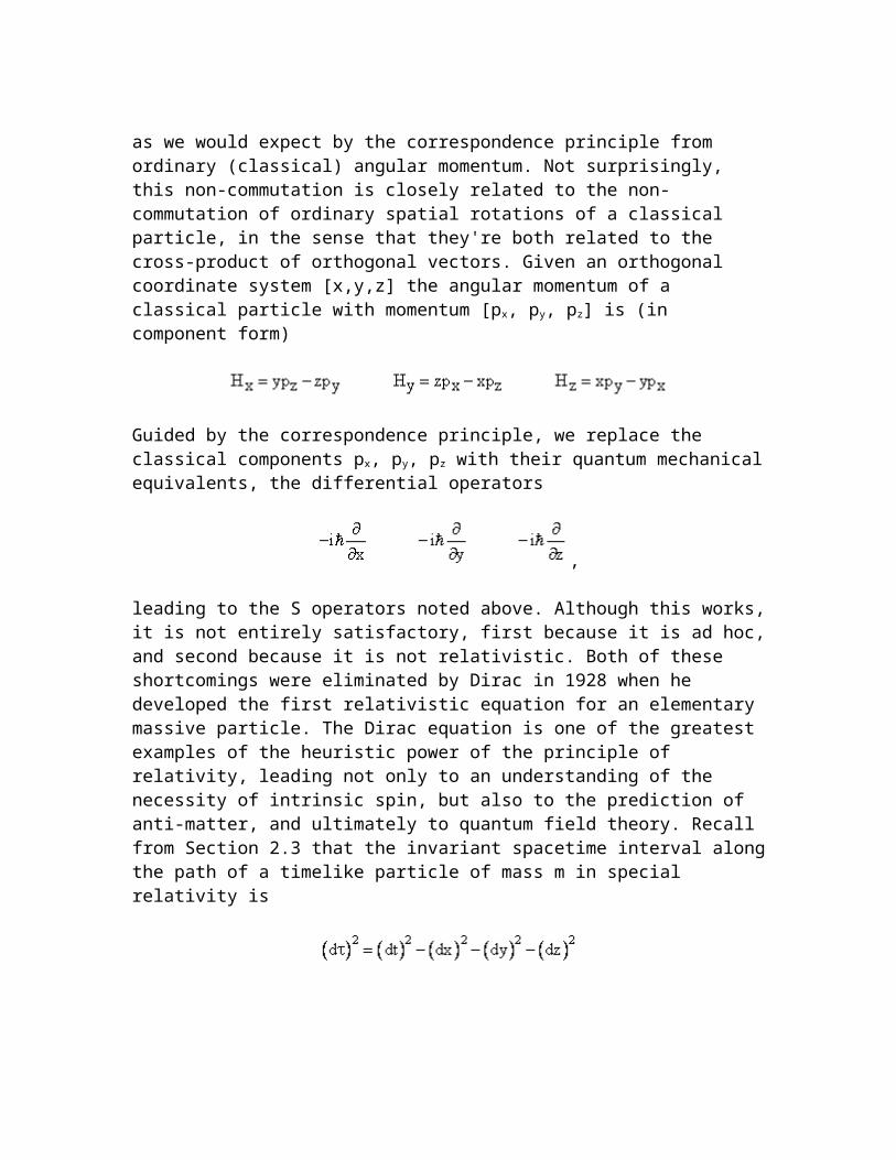
of motion that people (like Bell) apparently have in mind when they think of determinism. Following the ancients, many people tend to instinctively exempt "violent motions" – i.e., motions resulting from acts of living volition – when considering determinism. In fact, when Bell contemplated the possibility that determinism might also apply to himself and other living beings, he coined a different name for it, calling it “super-determinism”. Regarding the experimental tests of quantum entanglement he said 

One of the ways of understanding this business is to say that the world is super-deterministic. That not only is inanimate nature deterministic, but we, the experimenters who imagine we can choose to do one experiment rather than another, are also determined. If so, the difficulty which this experimental result creates disappears.

 But what Bell calls (admittedly on the spur of the moment) super-determinism is nothing other than what philosophers have always called simply determinism. Ironically, if confronted with the idea of vitalism, i.e., the notion that living beings are exempt from the normal laws of physics that apply to inanimate objects, or at least that living beings also entail some other kind of action transcending the normal laws of physics in physically observable ways – many physicists would probably be skeptical if not downright dismissive… and yet hardly any would think to question this very dualistic assumption underlying Bell’s analysis. Regardless of our conscious beliefs, it's psychologically very difficult for us to avoid bifurcating the world into inanimate objects that obey strict laws of causality, and animate objects (like ourselves) that do not. This dichotomy was historically appealing, and may even have been necessary for the development of classical physics, but it always left the nagging question of how or why we (and our constituent atoms) manage to evade the iron hand of determinism that governs everything else. This view affects our conception of science by suggesting to us that the experimenter is not himself part of nature, and is exempt from whatever determinism is postulated for the system being studied. Thus we imagine that we can "test" whether the universe is behaving deterministically by turning some dials and seeing how the universe responds, overlooking the fact that we and the dials are also part of the universe.  This immediately introduces "the measurement problem": Where do we draw the boundaries between separate phenomena? What is an observation? How do we distinguish "nature" from "violence", and is this distinction even warranted? When people say they're talking about a deterministic world, they're almost always not. What they're usually talking about is a deterministic sub-set of the world that can be subjected to freely chosen inputs from a non-deterministic "exterior". But just as with the measurement problem in quantum mechanics, when we think we've figured out the constraints on how a deterministic test apparatus can behave in response to arbitrary inputs, someone says "but isn't the whole lab a deterministic system?", and then the whole building, and so on. At what point does "the collapse of determinism" occur, so that we can introduce free inputs to test the system? Just as the infinite regress of the measurement problem in quantum mechanics leads to bewilderment, so too does the infinite regress of determinism.

 The other loop-hole that can never be closed is what Bell called "correlation by post-arrangement" or "backwards causality". I'd prefer to say that the system may violate the assumption of strong temporal asymmetry, but the point is the same. Clearly the causal pasts of the spacelike separated arms of an EPR experiment overlap, so all the objects involved share a common causal past. Therefore, without something to "block off" this region of common past from the emission and absorption events in the EPR experiment, we're not justified in asserting causal independence, which is required for Bell's derivation. The usual and, as far as I know, only way of blocking off the causal past is by injecting some "other" influence, i.e., an influence other than the deterministic effects propagating from the causal past. This "other" may be true randomness, free will, or some other concept of "free occurrence". In any case, Bell's derivation requires us to assert that each measurement is a "free" action, independent of the causal past, which is inconsistent with even the most limited construal of determinism. There is a fascinating parallel between the ancient concepts of natural and violent motion and the modern quantum mechanical concepts of the linear evolution of the wave function and the collapse of the wave function. These modern concepts are sometimes termed U, for unitary evolution of the quantum mechanical state vector, and R, for reduction of the state vector onto a particular basis of measurement or observation. One could argue that the U process corresponds closely with Aristotle's natural (inanimate) evolution, while the R process represents Aristotle's violent evolution, triggered by some living act. As always, we face the question of whether this is an accurate or meaningful bifurcation of events. Today there are several "non-collapse" interpretations of quantum mechanics, including the famous "many worlds" interpretation of Everett and DeWit. However, to date, none of these interpretations has succeeded in giving a completely satisfactory account of quantum mechanical processes, so we are not yet able to dispense with Aristotle's distinction between natural and violent motion. 9.7  Angels and Archetypes 

The Stranger is the preparer of the way of the quaternity which he follows. Women and children follow him gladly and he sometimes teaches them. He sees his surroundings and particularly me as ignorant and uneducated. He is no anti-Christ, but in a certain sense an anti-scientist…                                                                Pauli describing a dream to Anna Jung, 1950

 Impressed by the seemingly limitless scope and precision of Newton’s laws, some of his successors during the Enlightenment imagined a fully deterministic world. Newton himself had tried to forestall any such conclusion by often referring to an active role for the divine spirit in the workings of nature, especially in establishing the astonishingly felicitous “initial conditions”, but also in restoring the world’s vitality and order from time to time. Nevertheless, he couldn’t resist demonstrating the apparently perfect precision with which the observed phenomena (at least in celestial mechanics) adhered to the mathematical principles expressed by the laws of motion and gravity, and this was the

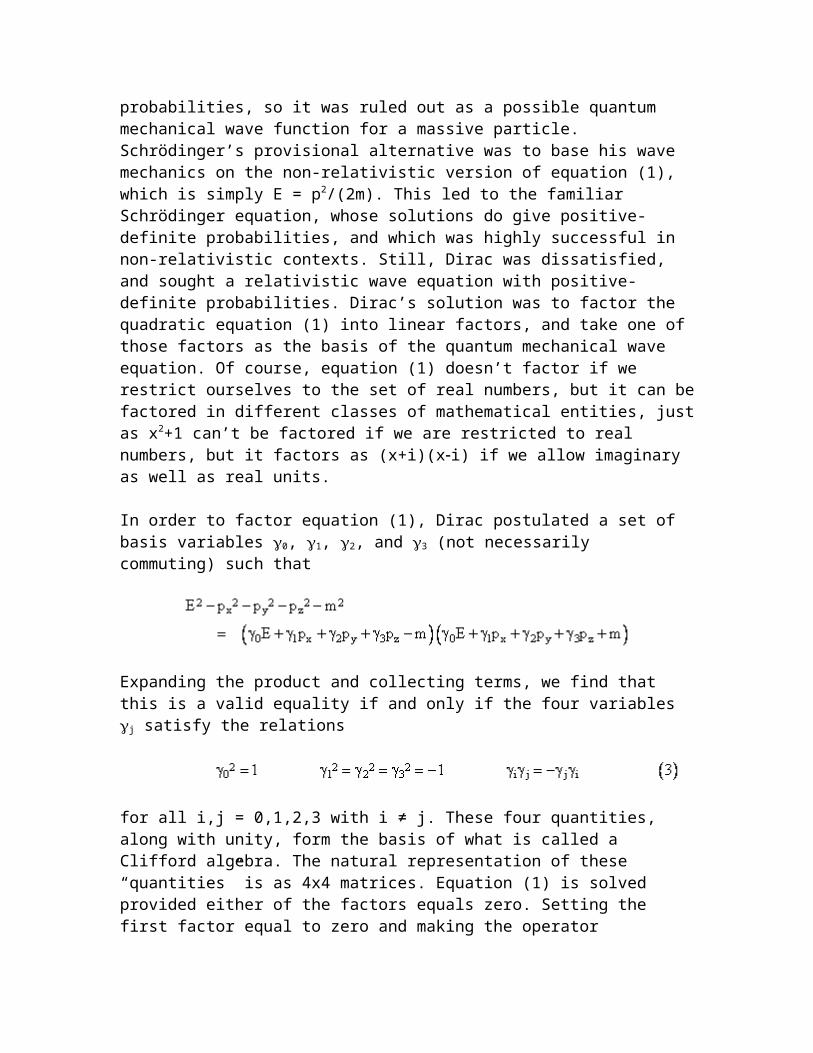
dominant impression given by his work. One of the most prominent and influential proponents of Newtonian determinism was Laplace, who famously wrote 

Present events are connected with preceding ones by the principle that a thing cannot occur without a cause which produces it. This axiom, known as the principle of sufficient reason, extends even to actions which are considered indifferent… We ought then to regard the present state of the universe as the effect of the anterior state and as the cause of the one that is to follow… If an intelligence, for one instant, recognizes all the forces which animate Nature, and the respective positions of the things which compose it, and if that intelligence is also sufficiently vast to subject these data to analysis, it will comprehend in one formula the movements of the largest bodies of the universe as well as those of the minutest atom. Nothing would be uncertain, and the future, as the past, would be present to its eyes.

 Notice that he initially conceives of determinism as a temporally ordered chain of implication, but then he describes a Gestalt shift, leading to the view of an atemporal "block universe" that simply exists. He doesn’t say so, but the concepts of time and causality in such a universe would be (at most) psychological interpretations, lacking any active physical significance, because in order for time and causality to be genuinely active, a degree of freedom is necessary; without freedom there can be no absolute direction of causal implication. For example, we ordinarily say that electromagnetic effects propagate at the speed of light, because the state of the electromagnetic field at any given event (time and place) is fully determined by the state of the field within the past light cone of that event, but since the laws of electromagnetism are time-symmetrical, the state of the field at any event is just as fully determined by state of the field within its future light cone, and by the state of the field on the same time slice as the event. We don’t conclude from this that electromagnetic effects therefore propagate instantaneously, let alone backwards in time. This example merely shows that when considering just a deterministic and time-symmetrical field, there is no unambiguous flow of information, because there can be no source of information in such a field. In order to even consider the flow of information, we must introduce a localized source of new information, i.e., an effect not implied by the field itself. Only then can we examine how this signal propagates through the field. Of course, although this signal is independent of the “past”, it is certainly not independent of the “future”. Owing to the time-symmetry of electromagnetism, we can begin with the effects and project “backwards” in time using the deterministic field equations to arrive at the supposedly freely produced signal. So even in this case, one can argue that the introduction of the signal was not a “free” act at all. We can regard it as a fully deterministic antecedent of the future, just as other events are regarded as fully deterministic consequences of the past. Acts that we regard are “free” are characterized by a kind of singularity, in the sense that when we extrapolate backwards from the effects to the cause, using the deterministic field laws, we reach a singularity at the cause, and cannot extrapolate through it back to a state that would precede it according to the deterministic field laws. The information emanating from a “free act”, when extrapolated

backwards from its effects to the source, must annihilate itself at the source. This is analogous to extrapolating the ripples in a pond backwards in time according to the laws of surface wave propagation, until reaching the event of a pebble entering the water, prior to which there is nothing in the quiet surface of the pond that implies (by the laws of the surface) the impending disturbance. Such backward accounts seem implausible, because they require such a highly coordinated arrangement of information from separate locations in the future, so we ordinarily prefer to conceive of the flow of information in the opposite direction.  Likewise, even in a block universe, it may be that certain directions are preferred based on the simplicity with which they can be described and conceptually grasped. For example, it may be possible to completely specify the universe based on the contents of a particular cross-sectional slice, together with a simple set of fixed rules for recursively inferring the contents of neighboring slices in a particular sequence, whereas other sequences may require a vastly more complicated “rule”. However, in a deterministic universe this chain of implication is merely a descriptive convenience, not an effective mechanism by which the events “come into being”. The concept of a static complete universe is consistent not only with the Newtonian physics discussed by Laplace, but also with the theory of relativity, in which the worldlines of objects (through spacetime) can be considered already existent in their entirety. In fact, it can be argued that this is a necessary interpretation for some general relativistic phenomena such as genuine black holes merging together in an infinite universe, because, as discussed in Section 7.2, the trousers model implies that the event horizons for two such black holes are continuously connected to each other in the future, as part of the global topology of the universe. There is no way for two black holes that are not connected to each other in the future to ever merge. This may sound tautological, but the global topological feature of the spacetime manifold that results in the merging of two black holes cannot be formed “from the past”, it must already be part of the final state of the universe. So, in this sense, relativity is perhaps an even more deterministic theory than Newtonian mechanics. The same conclusion could be reached by considering the lack of absolute simultaneity in special relativity, which makes it impossible to say which of two spacelike separated events preceded the other. Admittedly, the determinism of classical physics (including relativity) has sometimes been challenged, usually by pointing out that the long-term outcome of a physical process may be exponentially sensitive to the initial conditions. The concept of classical determinism relies on each physical variable being a real number (in the mathematical sense) representing and infinite amount of information. One can argue that this premise is implausible, and it certainly can’t be proven. We must also consider the possibility of singularities in classical physics, unless they are simply excluded on principle. Nevertheless, if the premise of infinite information in each real variable is granted, and if we exclude singularities, classical physics exhibits the distinctive feature of determinism. In contrast, quantum mechanics is widely regarded as decidedly non-deterministic. Indeed, as we saw in Section 9.6, there is a famous theorem of von Neumann that

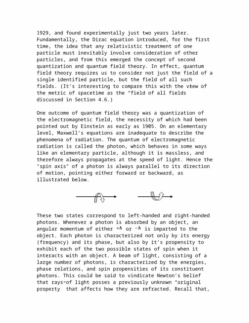
purports to rule out determinism (in the form of hidden variables) in the realm of quantum mechanics. However, as Einstein observed 

Whether objective facts are subject to causality is a question whose answer necessarily depends on the theory from which we start. Therefore, it will never be possible to decide whether the world is causal or not.

 The word “causal” is being used here as a synonym for deterministic, since Einstein had in mind strict causality, with no free choices, as summarized in his famous remark that “God does not play dice with the universe”. We've seen that von Neumann’s proof was based on a premise which is effectively equivalent to what he was trying to prove, nicely illustrating Einstein’s point that the answer depends on the theory from which we start. An assertion about what is recursively possible can be meaningful only if we place some constraints on the allowable recursive "algorithm". For example, the nth state vector of a system may be the kn+1 through k(n+1) digits of . This would be a perfectly deterministic system, but the relations between successive states would be extremely obscure. In fact, assuming the digits of the two transcendental numbers and e are normally distributed (as is widely believed, though not proven), any finite string of decimal digits occurs infinitely often in their decimal expansions, and each string occurs with the same frequency in both expansions. (It's been noted that, assuming normality, the digits of would make an inexhaustible source of high-quality "random" number sequences, higher quality than anything we can get out of conventional pseudo-random number generators). Therefore, given any finite number of digits (observations), we could never even decide whether the operative “algorithm” was or e, nor whether we had correctly identified the relevant occurrence in the expansion. Thus we can easily imagine a perfectly deterministic universe that is also utterly unpredictable. (Interestingly, the recent innovation that enables computation of the nth hexadecimal digit of (with much less work than required to compute the first n digits) implies that we could present someone with a sequence of digits and challenge them to determine where it first occurs in the decimal expansion of , and it may be practically impossible for them to find the answer.) Even worse, there need be no simple rule of any kind relating the events of a deterministic universe. This highlights the important distinction between determinism and the concepts of predictability and complexity. There is no requirement for a deterministic universe to be predictable, or for its complexity to be limited in any way. Thus, we can never prove that any finite set of observations could only have occurred in a non-deterministic algorithm. In a sense, this is trivially true, because a finite Turing machine can always be written to generate any given finite string, although the algorithm necessary to generate a very irregular string may be nearly as long as the string itself. Since determinism is inherently undecidable, we may try to define a more tractable notion, such as predictability, in terms of the exhibited complexity manifest in our observations. This could be quantified as the length of the shortest Turing machine required to reproduce our observations, and we might imagine that in a completely random universe, the size of the required algorithm would grow in proportion to the number of observations (as we are forced to include ad hoc modifications to the

algorithm to account for each new observation). On this basis it might seem that we could eventually assert with certainty that the universe is inherently unpredictable (on some level of experience), i.e., that the length of the shortest Turing machine required to duplicate the results grows in proportion with the number of observations. In a sense, this is what the "no hidden variables" theorems try to do. However, we can never reach such a conclusion, as shown by Chaitin's proof that there exists an integer k such that it's impossible to prove that the complexity of any specific string of binary bits exceeds k (where "complexity" is defined as the length of the smallest Turing program that generates the string). This is true in spite of the fact that "almost all" strings have complexity greater than k. Therefore, even if we (sensibly) restrict our meaningful class of Turing machines to those of complexity less than a fixed number k, rather than allowing the complexity of our model to increase in proportion to the number of observations, it's still impossible for any finite set of observations (even if we continue gathering data forever) to be provably inconsistent with a Turing machine of complexity less than k. Naturally we must be careful not to confuse the question of whether "there exist" sequences of complexity greater than k with the question of whether we can prove that any particular sequence has complexity greater than k. When Max Born retired from his professorship at the University of Edinburgh in 1953, a commemorative volume of scientific papers was prepared. Einstein contributed a paper, in which (as Born put it) Einstein’s “philosophical objection to the statistical interpretation of quantum mechanics is particularly cogently and clearly expressed”. The two men took up the subject in their private correspondence (which had started nearly 50 years earlier when they were close friends in Berlin during the first world war), and the ensuring argument strained their friendship nearly to the breaking point. Eventually they appealed to a mutual friend, Wolfgang Pauli, who tried to clarify the issues. Born was sure that Einstein’s critique of quantum mechanics was focused on the lack of determinism, but Pauli explained (with the benefit of discussing the matter with Einstein personally at Princeton) that this was not the case. Pauli wrote to Born that 

Einstein does not consider the concept of ‘determinism’ to be as fundamental as it is frequently held to be (as he told me emphatically many times), and he denied energetically that he ever put up a postulate such as (your letter, para 3) ‘the sequence of such conditions must also be objective and real, that is, automatic, machine-like, deterministic’. In the same way, he disputes that he uses as criterion for the admissibility of a theory the question ‘Is it rigorously deterministic?’

 This should not be surprising, given that Einstein knew it is impossible to ever decide whether or not the world is deterministic. Pauli went on to explain the position that Einstein himself had already described in the EPR paper years earlier, i.e., the insistence on what might be called complete realism. Pauli summarized his understanding of Einstein’s view, along with his own response to it, in the letter to Born, in which he tried to explain why he thought it was “misleading to bring the concept of determinism into the dispute with Einstein”. He wrote 

Einstein would demand that the 'complete real description of the System', even before an observation, must already contain elements which would in some way correspond with the possible differences in the results of the observations. I think, on the other hand, that this postulate is inconsistent with the freedom of the experimenter to select mutually exclusive experimental arrangements…

 Born accepted Pauli’s appraisal of the dispute, and conceded that he (Born) had been wrong in thinking Einstein’s main criterion was determinism. Born’s explanation of his misunderstanding was that he simply couldn’t believe Einstein would demand a “complete real description” beyond that which can be perceived. The great lesson that Born, Heisenberg, and the other pioneers of quantum mechanics had taken from Einstein’s early work on special relativity was that we must insist on operational definitions for all the terms of a scientific theory, and deny meaning to concepts or elements of a theory that have no empirical content. But Einstein did not hold to that belief, and even chided Born for adopting the positivistic maxim esse est percepi.  There is, however, a certain irony in Pauli’s position, since he asserts the irrelevance of the concept of determinism, but at the same time criticizes Einstein’s “postulate” by saying that it is “inconsistent with the freedom of the experimenter to select mutually exclusive experimental arrangements”. As discussed in the previous section, this freedom is itself a postulate, an unproveable proposition, and one that is obviously inconsistent with determinism. Einstein argued that determinism is an undecidable proposition in the absolute sense, and hence not a suitable criterion for physical theories, whereas Born and Pauli implicitly demanded non-determinism of a physical theory.  By the way, Pauli and his psychoanalyst Carl Jung spent much time developing a concept which they called synchronicity, loosely defined as the coincidental occurrence of non-causally related events that nevertheless exhibit seemingly meaningful correlations. This was presented as a complementary alternative to the more scientific principle of causation. One notable example of synchronicity was the development of the concept of synchronicity itself, along side Einstein’s elucidation of non-classical correlations between distant events implied by quantum mechanics. But Pauli (like Born) didn’t place any value on Einstein’s “realist” reasons for rejecting their quantum mechanics as a satisfactory theory. Pauli wrote to Born 

One should no more rack one’s brain about the problem of whether something one cannot know anything about exists all the same, than about the ancient question of how many angels are able to sit on the point of a needle. But it seems to me that Einstein’s questions are ultimately always of this kind.

 It’s interesting that Pauli referred to the question of how many angles can sit on the point of a needle, since one of his most important contributions to quantum mechanics was the exclusion principle, which in effect answered the question of how many electrons can fit into a single quantum state. He and Jung might have cited this as an example of the collective unconscious reaching back to the scholastic theologians. Pauli seems to given credence to Jung’s theory of archetypes, according to which the same set of organizing

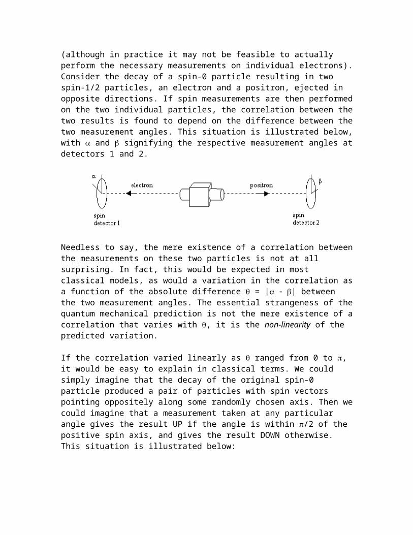
principles and forms (the “unus mundus”) that govern the physical world also shape the human mind, so there is a natural harmony between physical laws and human thoughts. To illustrate this, Pauli wrote an essay on Kepler, which was published along with Jung’s treatise on synchronicity. The complementarity interpretation of quantum mechanics, developed by Bohr, can be seen as an attempted compromise with Einstein over his demand for realism (similar to Einstein’s effort to reconcile relativity with the language of Lorentz’s ether). Two requirements of a classical description of phenomena are that they be strictly causal and that they be expressed in terms of space and time. According to Bohr, these two requirements are mutually exclusive. As summarized by Heisenberg 

There exists a body of exact mathematical laws, but these cannot be interpreted as expressing simple relationships between objects existing in space and time. The observable predictions of this theory can be approximately described in such terms, but not uniquely… This is a direct result of the indeterminateness of the concept “observation”. It is not possible to decide, other than arbitrarily, what objects are to be considered as part of the observed system and what as part of the observer’s apparatus.  The concept “observation” … can be carried over to atomic phenomena only when due regard is paid to the limitations placed on all space-time descriptions by the uncertainty principle.

 Thus any description of events in terms of space and time must include acausal aspects, and conversely any strictly causal description cannot be expressed in terms of space and time. This of course was antithetical to Einstein, who maintained that the general theory of relativity tells us something exact about space and time. (He wrote in 1949 that “In my opinion the equations of general relativity are more likely to tell us something precise than all other equations of physics”.) To accept that the fundamental laws of physics are incompatible with space and time would require him to renounce general relativity. He occasionally contemplated the possibility that this step might be necessary, but never really came to accept it. He continued to seek a conceptual framework that would allow for strictly causal descriptions of objects in space and time – even if it required the descriptions to involve purely hypothetical components. In this respect his attitude resembled that of Lorentz, who, in his later years, continued to argue for the conceptual value of the classical ether and absolute time, even though he was forced to concede that they were undetectable. 9.8  Quaedam Tertia Natura Abscondita 

The square root of 9 may be either +3 or -3, because a plus times a plus or a minus times a minus yields a plus. Therefore the square root of -9 is neither +3 nor -3, but is a thing of some obscure third nature.                                                                                                Girolamo Cardano, 1545

 

In a certain sense the peculiar aspects of quantum spin measurements in EPR-type experiments can be regarded as a natural extension of the principle of special relativity. Classically a particle has an intrinsic spin about some axis with an absolute direction, and the results of measurements depend on the difference between this absolute spin axis and the absolute measurement axis. In contrast, quantum theory says there are no absolute spin angles, only relative spin angles. In other words, the only angles that matter are the differences between two measurements, whose absolute values have no physical significance. Furthermore, the relations between measurements vary in a non-linear way, so it's not possible to refer them to any absolute direction.  This "relativity of angular reference frames" in quantum mechanics closely parallels the relativity of translational reference frames in special relativity. This shouldn’t be too surprising, considering that velocity “boosts” are actually rotations through imaginary angles. Recall from Section 2.4 that the relationship between the frequencies of a given signal as measured by the emitter and absorber depends on the two individual speeds ve and va relative to the medium through which the signal propagates at the speed cs, but as this speed approaches c (the speed of light in a vacuum), the frequency shift becomes dependent only on a single variable, namely, the mutual speed between the emitter and absorber relative to each other. This degeneration of dependency from two independent “absolute” variables down to a single “relative” variable is so familiar today that we take it for granted, and yet it is impossible to explain in classical Newtonian terms. Schematically we can illustrate this in terms of three objects in different translational frames of reference as shown below: 

 The object B is stationary (corresponding to the presumptive medium of signal propagation), while objects A and C move relative to B in opposite directions at high speed. Intuitively we would expect the velocity of A in terms of the rest frame of C (and vice versa) to equal the sum of the velocities of A and C in terms of the rest frame of B. If we allowed the directions of motion to be oblique, we would still have the “triangle inequality” placing limits on how the mutual speeds are related to each other. This could be regarded as something like a “Bell inequality” for translational frames of reference. When we measure the velocity of A in terms of the rest frame of C we find that it does not satisfy this additive property, i.e., it violates "Bell's inequality" for special relativity. Compare the above with the actual Bell's inequality for entangled spin measurements in quantum mechanics. Two measurements of the separate components of an entangle pair may be taken at different orientations, say at the angles A and C, relative to the presumptive common spin axis of the pair, as shown below: 

 We then determine the correlations between the results for various combinations of measurement angles at the two ends of the experiment. Just as in the case of frequency measurements taken at two different boost angles, the classical expectation is that the correlation between the results will depend on the two measurement angles relative to some reference direction established by the mechanism. But again we find that the correlations actually depend only on the single difference between angles A and C, not on their two individual values relative to some underlying reference. The close parallel between the “boost inequalities” in special relativity and the Bell inequalities for spin measurements in quantum mechanics is more than just superficial.  In both cases we find that the assumption of an absolute frame (angular or translational) leads us to expect a linear relation between observable qualities, and in both cases it turns out that in fact only the relations between one realized event and another, rather than between a realized event and some absolute reference, govern the outcomes. Recall from Section 9.5 that the correlation between the spin measurements (of entangled spin-1/2 particles) is simply -cos() where is the relative spatial angle between the two measurements. The usual presumption is that the measurement devices are at rest with respect to each other, but if they have some non-zero relative velocity v,  we can represent the "boost" as a complex rotation through an angle = arctanh(v) where arctanh is the inverse hyperbolic tangent (see Part 6 of the Appendix). By analogy, we might expect the "correlation" between measurements performed with respect to two basis systems with this relative angle would be 

 which of course is Lorentz-Fitzgerald factor that scales the transformation of space and time intervals from one system of inertial coordinates to another, leading to the relativistic Doppler effect, and so on. In other words, this factor represents the projection of intervals in one frame onto the basis axes of another frame, just as the correlation between the particle spin measurements is the projection of the spin vector onto the respective measurement bases. Thus the "mysterious" and "spooky" correlations of quantum mechanics can be placed in close analogy with the time dilation and length contraction effects of special relativity, which once seemed equally counterintuitive. The

spinor representation, which uses complex numbers to naturally combine spatial rotations and "boosts" into a single elegant formalism, was discussed in Section 2.6.  In this context we can formulate a generalized "EPR experiment" allowing the two measurement bases to differ not only in spatial orientation but also by a boost factor, i.e., by a state of relative motion.  The resulting unified picture shows that the peculiar aspects of quantum mechanics can, to a surprising extent, be regarded as aspects of special relativity. In a sense, relativity and quantum theory could be summarized as two different strategies for accommodating the peculiar wave-particle duality of physical phenomena. One of the problems this duality presented to classical physics was that apparently light could either be treated as an inertial particle emitted at a fixed speed relative to the source, ala Newton and Ritz, or it could be treated as a wave with a speed of propagation fixed relative to the medium and independent of the source, ala Maxwell. But how can it be both? Relativity essentially answered this question by proposing a unified spacetime structure with an indefinite metric (viz, a pseudo-Riemannian metric). This is sometimes described by saying time is imaginary, so its square contributes negatively to the line element, and yields an invariant null-cone structure for light propagation, yielding invariant light speed. But waves and particles also differ with regard to interference effects, i.e., light can be treated as a stream of inertial particles with no interference (though perhaps "fits and starts) ala Newton, or as a wave with fully wavelike interference effects, ala Huygens.  Again the question was how to account for the fact that light exhibits both of these characteristics. Quantum mechanics essentially answered this question by proposing that observables are actually expressible in terms of probability amplitudes, and these amplitudes contain an imaginary component which, upon taking the norm, can contribute negatively to the probabilities, yielding interference effects. Thus we see that both of these strategies can be expressed in terms of the introduction of imaginary (in the mathematical sense) components in the descriptions of physical phenomena, yielding the possibility of cancellations in, respectively, the spacetime interval and superposition probabilities (i.e., interference). They both attempt to reconcile aspects of the wave-particle duality of physical entities. The intimate correspondence between relativity and quantum theory was not lost on Niels Bohr, who remarked in his Warsaw lecture in 1938 

Even the formalisms, which in both theories within their scope offer adequate means of comprehending all conceivable experience, exhibit deep-going analogies. In fact, the astounding simplicity of the generalisation of classical physical theories, which are obtained by the use of multidimensional [non-positive-definite] geometry and non-commutative algebra, respectively, rests in both cases essentially on the introduction of the conventional symbol sqrt(-1).   The abstract character of the formalisms concerned is indeed, on closer examination, as typical of relativity theory as it is of quantum mechanics, and it is in this respect purely a matter of tradition if the former theory is considered as a completion of classical physics rather than as a first fundamental step in the

thorough-going revision of our conceptual means of comparing observations, which the modern development of physics has forced upon us.

 Of course, Bernhardt Riemann, who founded the mathematical theory of differential geometry that became general relativity, also contributed profound insights to the theory of complex functions, the Riemann sphere (Section 2.6), Riemann surfaces, and so on. (Here too, as in the case of differential geometry, Riemann built on and extended the ideas of Gauss, who was among the first to conceive of the complex number plane.) More recently, Roger Penrose has argued that some “complex number magic” seems to be at work in many of the most fundamental physical processes, and his twistor formalism is an attempt to find a framework for physics that exploits this the special properties of complex functions at a fundamental level. Modern scientists are so used to complex numbers that, in some sense, the mystery is now reversed. Instead of being surprised at the physical manifestations of imaginary and complex numbers, we should perhaps wonder at the preponderance of realness in the world. The fact is that, although the components of the state vector in quantum mechanics are generally complex, the measurement operators are all required – by fiat – to be Hermitian, meaning that they have strictly real eigenvalues. In other words, while the state of a physical system is allowed to be complex, the result of any measurement is always necessarily real. So we can’t claim that nature is indifferent to the distinction between real and imaginary numbers. This suggests to some people a connection between the “measurement problem” in quantum mechanics and the ontological status of imaginary numbers. The striking similarity between special relativity and quantum mechanics can be traced to the fact that, in both cases, two concepts that were formerly regarded as distinct and independent are found not to be so. In the case of special relativity, the two concepts are space and time, whereas in quantum mechanics the two concepts are position and momentum. Not surprisingly, these two pairs of concepts are closely linked, with space corresponding to position, and time corresponding to momemtum (the latter representing the derivative of position with respect to time). Considering the Heisenberg uncertainty relation, it’s tempting to paraphrase Minkowski’s famous remark, and say that henceforth position by itself, and momentum by itself, are doomed to fade away into mere shadows, and only a kind of union of the two will preserve an independent reality. 9.9  Locality and Temporal Asymmetry 

All these fifty years of conscious brooding have brought me no nearer to the answer to the question, 'What are light quanta?' Nowadays every Tom, Dick and Harry thinks he knows it, but he is mistaken.                                                                                                                 Einstein, 1954

 We've seen that the concept of locality plays an important role in the EPR thesis and the interpretation of Bell's inequalities, but what precisely is the meaning of locality,

especially in a quasi-metric spacetime in which the triangle inequality doesn't hold? The general idea of locality in physics is based on some concept of nearness or proximity, and the assertion that physical effects are transmitted only between suitably "nearby" events. From a relativistic standpoint, locality is often defined as the proposition that all causal effects of a particular event are restricted to the interior (or surface) of the future null cone of that event, which effectively prohibits communication between spacelike-separated events (i.e., no faster-than-light communication). However, this restriction clearly goes beyond a limitation based on proximity, because it specifies the future null cone, thereby asserting a profound temporal asymmetry in the fundamental processes of nature. What is the basis of this asymmetry? It certainly is not apparent in the form of the Minkowski metric, nor in Maxwell's equations. In fact, as far as we know, all the fundamental processes of nature are perfectly time-symmetric, with the single exception of certain processes involving the decay of neutral kaons. However, even in that case, the original experimental evidence in 1964 for violation of temporal symmetry was actually a demonstration of asymmetry in parity and charge conjugacy, from which temporal asymmetry is indirectly inferred on the basis of the CPT Theorem. As recently as 1999 there were still active experimental efforts to demonstrate temporal asymmetry directly. In any case, aside from the single rather subtle peculiarity in the behavior of neutral kaons, no one has ever found any evidence at all of temporal asymmetry in any fundamental interaction. How, then, do we justify the explicit temporal asymmetry in our definition of locality for all physical interactions? As an example, consider electromagnetic interactions, and recall that the only invariant measure of proximity (nearness) in Minkowski spacetime is the absolute interval  

 which is zero between the emission and absorption of a photon. Clearly, any claim that influence can flow from the emission event to the absorption event but not vice versa cannot be based on an absolute concept of physical nearness. Such a claim amounts to nothing more or less than an explicit assertion of temporal asymmetry for the most fundamental interactions, despite the complete lack of justification or evidence for such asymmetry in photon interactions. Einstein commented on the unnaturalness of irreversibility in fundamental interactions in a 1909 paper on electromagnetic radiation, in which he argued that the asymmetry of the elementary process of radiation according to the classical wave theory of light was inconsistent with what we know of other elementary processes. 

While in the kinetic theory of matter there exists an inverse process for every process in which only a few elementary particles take part (e.g., for every molecular collision), according to the wave theory this is not the case for elementary radiation processes. According to the prevailing theory, an oscillating ion produces an outwardly propagated spherical wave. The opposite process does not exist as an elementary process. It is true that the inwardly propagated

spherical wave is mathematically possible, but its approximate realization requires an enormous number of emitting elementary structures. Thus, the elementary process of light radiation as such does not possess the character of reversibility. Here, I believe, our wave theory is off the mark. Concerning this point the Newtonian emission theory of light seems to contain more truth than does the wave theory, since according to the former the energy imparted at emission to a particle of light is not scattered throughout infinite space but remains available for an elementary process of absorption.

 In the same paper he wrote 

For the time being the most natural interpretation seems to me to be that the occurence of electromagnetic fields of light is associated with singular points just like the occurence of electrostatic fields according to the electron theory. It is not out of the question that in such a theory the entire energy of the electromagnetic field might be viewed as localized in these singularities, exactly like in the old theory of action at a distance.

 This is a remarkable statement coming from Einstein, considering his deep commitment to the ideas of locality and the continuum. The paper is also notable for containing his premonition about the future course of physics: 

Today we must regard the ether hypothesis as an obsolete standpoint. It is undeniable that there is an extensive group of facts concerning radiation that shows that light possesses certain fundamental properties that can be understood far more readily from the standpoint of Newton's emission theory of light than from the standpoint of the wave theory. It is therefore my opinion that the next stage in the development of theoretical physics will bring us a theory of light that can be understood as a kind of fusion of the wave and emission theories of light.

 Likewise in a brief 1911 paper on the light quantum hypothesis, Einstein presented reasons for believing that the propagation of light consists of a finite number of energy quanta which move without dividing, and can be absorbed and generated only as a whole. Subsequent developments (quantum electrodynamics) have incorporated these basic insights, leading us to regard a photon (i.e., an elementary interaction) as an indivisible whole, including the null-separated emission and absorption events on a symmetrical footing. This view is supported by the fact that once a photon is emitted, its quantum phase does not advance while "in flight", because quantum phase is proportional to the absolute spacetime interval, which, as discussed in Section 2.1, is what gives the absolute interval its physical significance. If we take seriously the spacetime interval as the absolute measure of proximity, then the transmission of a photon is, in some sense, a single event, coordinated mutually and symmetrically between the points of emission and absorption. This image of a photon as a single unified event with a coordinated emission and absorption seems unsatisfactory to many people, partly because it doesn't allow for the

concept of a "free photon", i.e., a photon that was never emitted and is never absorbed. However, it's worth remembering that we have no direct experience of "free photons", nor of any "free particles", because ultimately all our experience is comprised of completed interactions. (Whether this extends to gravitational interactions is an open question.) Another possible objection to the symmetrical view of elementary interactions is that it doesn't allow for a photon to have wave properties, i.e., to have an evolving state while "in flight", but this objection is based on a misconception. From the standpoint of quantum electrodynamics, the wave properties of electromagnetic radiation are actually wave properties of the emitter. All the potential sources of a photon have a certain (complex) amplitude for photon emission, and this amplitude evolves in time as we progress along the emitter's worldline. However, as noted above, once a photon is emitted, its phase does not advance. In a sense, the ancients who conceived of sight as something like a blind man's incompressible cane, feeling distant objects, were correct, because our retinas actually are in "direct" contact, via null intervals, with the sources of light. The null interval plays the role of the incompressible cane, and the wavelike properties we "feel" are really the advancing quantum phases of the source. One might think that the reception amplitude for an individual photon must evolve as a function of its position, because if we had (contra-factually) encountered a particular photon one meter further away from its source than we did, we would surely have found it with a different phase. However, this again is based on a misconception, because the photon we would have received one meter further away (on the same timeslice) would necessarily have been emitted one light-meter earlier, carrying the corresponding phase of the emitter at that point on its worldline. When we consider different spatial locations relative to the emitter, we have to keep clearly in mind which points they correspond to along the worldline of the emitter.  Taking another approach, it might seem that we could "look at" a single photon at different distances from the emitter (trying to show that its phase evolves in flight) by receding fast enough from the emitter so that the relevant emission event remains constant, but of course the only way to do this would be to recede at the speed of light (i.e., along a null interval), which isn't possible. This is just a variation of the young Einstein's thought experiment about how a "standing wave" of light would appear to someone riding along side it. The answer, of course, is that it’s not possible for a material object to move along-side a pulse of light (in vacuum), because light exists only as completed interactions on null intervals. If we attempted such an experiment, we would notice that, as our speed of recession from the source gets closer to c, the difference between the phases of the photons we receive becomes smaller (i.e., the "frequency" of the light gets red-shifted), and approaches zero, which is just what we should expect based on the fact that each photon is simply the lightlike null projection of the emitter's phase at a point on the emitter's worldline. Hence, if we stay on the same projection ray (null interval), we are necessarily looking at the same phase of the emitter, and this is true everywhere on that null ray. This leads to the view that the concept of a "free photon" is meaningless, and a photon is nothing but the communication of an emitter event's phase to some null-separated absorber event, and vice versa.  

More generally, since the Schrodinger wave function propagates at c, it follows that every fundamental quantum interaction can be regarded as propagating on null surfaces. Dirac gave an interesting general argument for this strong version of Huygens' Principle in the context of quantum mechanics. In his "Principles of Quantum Mechanics" he noted that a measurement of a component of the instantaneous velocity of a free electron must give the value c, which implies that electrons (and massive particles in general) always propagate along null intervals, i.e., on the local light cone. At first this may seem to contradict the fact that we observe massive objects to move at speeds much less than the speed of light, but Dirac points out that observed velocities are always average velocities over appreciable time intervals, whereas the equations of motion of the particle show that its velocity oscillates between +c and -c in such a way that the mean value agrees with the average value. He argues that this must be the case in any relativistic theory that incorporates the uncertainty principle, because in order to measure the velocity of a particle we must measure its position at two different times, and then divide the change in position by the elapsed time. To approximate as closely as possible to the instantaneous velocity, the time interval must go to zero, which implies that the position measurements must approach infinite precision. However, according to the uncertainty principle, the extreme precision of the position measurement implies an approach to infinite indeterminancy in the momentum, which means that almost all values of momentum - from zero to infinity - become equally probable. Hence the momentum is almost certainly infinite, which corresponds to a speed of c. This is obviously a very general argument, and applies to all massive particles (not just fermions). This oscillatory propagation on null cones is discussed further in Section 9.11. Another argument that seems to favor a temporally symmetric view of fundamental interactions comes from consideration of the exchange of virtual photons. (Whether virtual particles deserve to be called "real" particles is debatable; many people prefer to regard them only as sometimes useful mathematical artifacts, terms in the expansion of the quantum field, with no ontological status. On the other hand, it's possible to regard all fundamental particles that way, so in this respect virtual particles are not unique.) The emission and absorption points of virtual particles may be space-like separated, and we therefore can't say unambiguously that one happened "before" the other. The temporal order is dependent on the reference frame. Surely in these circumstances, when it's not even possible to say absolutely which side of the interaction was the emission and which was the absorption, those who maintain that fundamental interactions possess an inherent temporal asymmetry have a very difficult case to make. Over limited ranges, a similar argument applies to massive particles, since there is a non-negligible probability of a particle traversing a spacelike interval if it's absolute magnitude is less than about h2/(2m)2, where h is Planck's constant and m is the mass of the particle. So, if virtual particle interactions are time-symmetric, why not all fundamental particle interactions? (Needless to say, time-symmetry of fundamental quantum interactions does not preclude asymmetry for macroscopic processes involving huge numbers of individual quantum interactions evolving from some, possibly very special, boundary conditions.) Experimentally, those who argue that the emission of a photon is conditioned by its absorption can point to the results from tests of Bell's inequalities, because the observed

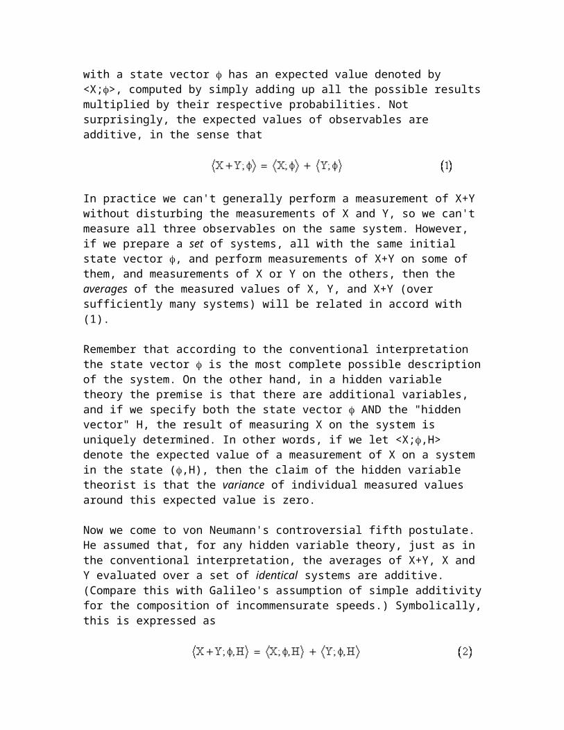
violations of those inequalities are exactly what the symmetrical model of interactions would lead us to expect. Nevertheless, the results of those experiments are rarely interpreted as lending support to the symmetrical model, apparently because temporal asymmetry is so deeply ingrained in peoples' intuitive conceptions of locality, despite the fact that there is very little (if any) direct evidence of temporal asymmetry in any fundamental laws or interactions.  Despite the preceding arguments in favor of symmetrical (reversible) fundamental processes, there are clearly legitimate reasons for being suspicious of unrestricted temporal symmetry. If it were possible for general information to be transmitted efficiently along the past null cone of an event, this would seem to permit both causal loops and causal interactions with spacelike-separated events, as illustrated below. 

 On such a basis, it might seem as if the Minkowskian spacetime manifold would be incapable of supporting any notion of locality at all. That triangle inequality fails in this manifold, so there are null paths connecting every two points, and this applies even to spacelike separated points if we allow the free flow of information in either direction along null surfaces. Indeed this seems to have been the main source of Einstein’s uneasiness with the “spooky” entanglements entailed by quantum theory. In a 1948 letter to Max Born, Einstein tried to clearly articulate his concern with entanglement, which he regarded as incompatible with “the confidence I have in the relativistic group as representing a heuristic limiting principle”. 

It is characteristic of physical objects [in the world of ideas] that they are thought of as arranged in a space-time continuum. An essential aspect of this arrangement of things in physics is that they lay claim, at a certain time, to an existence independent of one another, provided these objects ‘are situated in different parts of space’. Unless one makes this kind of assumption about the independence of the existence (the 'being-thus') of objects which are far apart from one another in space… the idea of the existence of (quasi) isolated systems, and thereby the postulation of laws which can be checked empirically in the accepted sense, would become impossible.

 In essence, he is arguing that without the assumption that it is possible to localize physical systems, consistent with the relativistic group, in such a way that they are

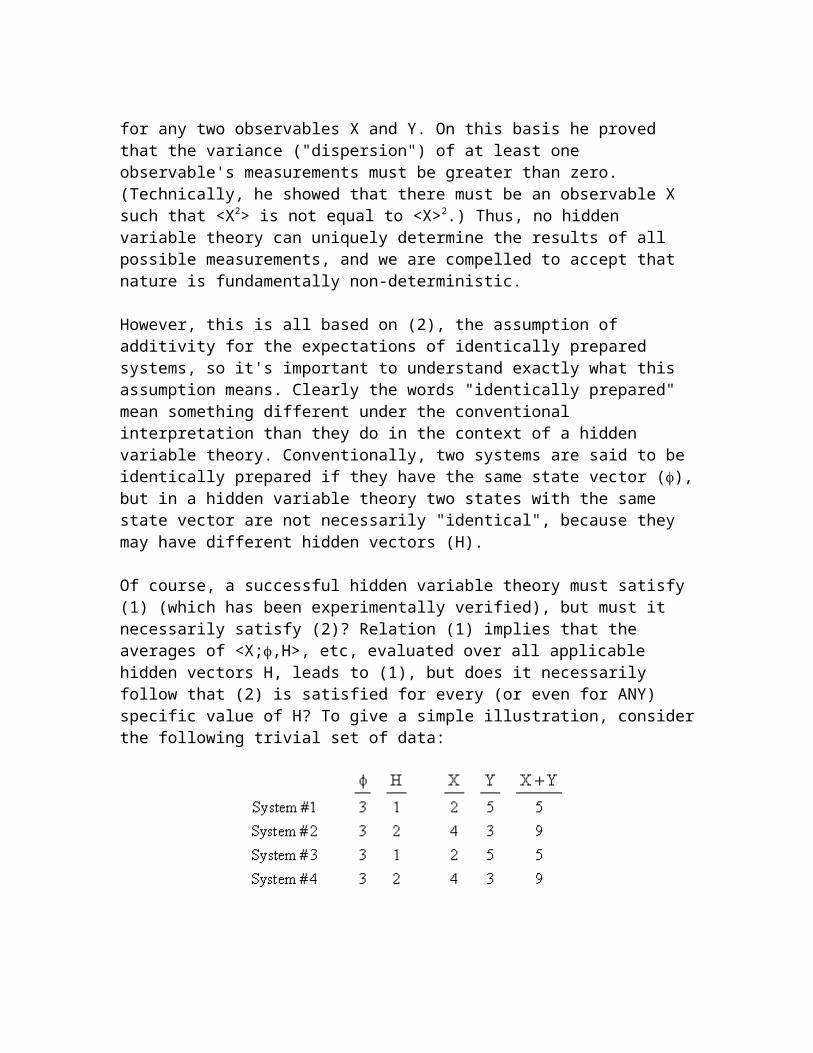
causally isolated, we cannot hope to analyze events in any effective way, such that one thing can be checked against another. After describing how quantum mechanics leads unavoidably to entanglement of potentially distant objects, and therefore dispenses with the principle of locality (in Einstein’s view), he says 

When I consider the physical phenomena known to me, even those which are being so successfully encompased by quantum mechanics, I still cannot find any fact anywhere which would make it appear likely that the requirement [of localizability] will have to be abandoned.

 At this point the precise sense in which quantum mechanics entail non-classical “influences” (or rather, correlations) for space-like separated events had not yet been clearly formulated, and the debate between Born and Einstein suffered (on both sides) from this lack of clarity. Einstein seems to have intuited that quantum mechanics does indeed entail distant correlations that are inconsistent with very fundamental classical notions of causality and independence, but he was unable to formulate those correlations clearly. For his part, Born outlined a simple illustration of quantum correlations occuring in the passage of light rays through polarizing filters – which is exactly the kind of experiment that, twenty years later, provided an example of the very thing that Einstein said he had been unable to find, i.e., a fact which makes it appear that the requirement of localizability must be abandoned. It’s unclear to what extent Born grasped the non-classical implications of those phenomena, which isn’t surprising, since the Bell inequalities had not yet been formulated. Born simply pointed out that quantum mechanics allows for coherence, and said that “this does not go too much against the grain with me”.  Born often argued that classical mechanics was just as probabilistic as quantum mechanics, although his focus was on chaotic behavior in classical physics, i.e., exponential sensitivity to initial conditions, rather than on entanglement. Born and Einstein often seemed to be talking past each other, since Born focused on the issue of determinism, whereas Einstein’s main concern was localizability. Remarkably, Born concluded his reply by saying 

I believe that even the days of the relativistic group, in the form you gave it, are numbered.

 One might have thought that experimental confirmation of quantum entanglement would have vindicated Born’s forecast, but we now understand that the distant correlations implied by quantum mechanics (and confirmed experimentally) are of a subtle kind that do not violate the “relativistic group”. This seems to be an outcome that neither Einstein nor Born anticipated; Born was right that the distant entanglement implicit in quantum mechanics would be proven correct, but Einstein was right that the relativistic group would emerge unscathed. But how is this possible? Considering that non-classical distant correlations have now been experimentally established with high confidence, thereby undermining the classical notion of localizability, how can we account for the continued ability of physicists to formulate and test physical laws?

 The failure of the triangle inequality (actually, the reversal of it) does not necessarily imply that the manifold is unable to support non-trivial structure. There are absolute distinctions between the sets of null paths connecting spacelike separated events and the sets of null paths connecting timelike separated events, and these differences might be exploited to yield a structure that conforms with the results of observation. There is no reason this cannot be a "locally realistic" theory, provided we understand that locality in a quasi-metric manifold is non-transitive. Realism is simply the premise that the results of our measurements and observations are determined by an objective world, and it's perfectly possible that the objective world might possess a non-transitive locality, commensurate with the non-transitive metrical aspects of Minkowski spacetime. Indeed, even before the advent of quantum mechanics and the tests of Bell's inequality, we should have learned from special relativity that locality is not transitive, and this should have led us to expect non-Euclidean connections and correlations between events, not just metrically, but topologically as well. From this point of view, many of the seeming paradoxes associated with quantum mechanics and locality are really just manifestations of the non-intuitive fact that the manifold we inhabit does not obey the triangle inequality (which is one of our most basic spatio-intuitions), and that elementary processes are temporally reversible. On the other hand, we should acknowledge that the Bell correlations can't be explained in a locally realistic way simply by invoking the quasi-metric structure of Minkowski spacetime, because if the timelike processes of nature were ontologically continuous it would not be possible to regard them as propagating on null surfaces. We also need our fundamental physical processes to consist of irreducible discrete interactions, as discussed in Section 9.10. 9.10  Spacetime Mediation of Quantum Interactions 

No reasonable definition of reality could be expected to permit this.                                                                Einstein, Podolsky, and Rosen, 1935

 According to general relativity the shape of spacetime determines the motions of objects while those objects determine (or at least influence) the shape of spacetime. Similarly in electrodynamics the fields determine the motions of charges in spacetime while the charges determine the fields in spacetime. This dualistic structure naturally arises when we replace action-at-a-distance with purely local influences in such a way that the interactions between "separate" objects are mediated by an entity extending between them. We must then determine the dynamical attributes of this mediating entity, e.g., the electromagnetic field in electrodynamics, or spacetime itself in general relativity. However, many common conceptions regarding the nature and extension of these mediating entities are called into question by the apparently "non-local" correlations in quantum mechanics, as highlighted by EPR experiments. The apparent non-locality of these phenomena arises from the fact that although we regard spacetime as metrically Minkowskian, we continue to regard it as topologically Euclidean. As discussed in the

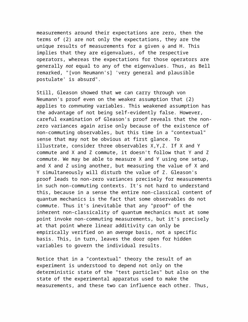
preceding sections, the observed phenomena are more consistent with a completely Minkowskian spacetime, in which physical locality is directly induced by the pseudo-metric of spacetime. According to this view, spacetime operates on matter via interactions, and matter defines for spacetime the set of allowable interactions, i.e., consistent with conservation laws. A quantum interaction is considered to originate on (or be "mediated" by) the locus of spacetime points that are null-separated from each of the interacting sites. In general this locus is a quadratic surface in spacetime, and its surface area is inversely proportional to the mass of the transferred particle.  For two timelike-separated events A and B the mediating locus is a closed surface as illustrated below (with one of the spatial dimensions suppressed) 

 The mediating surface is shown here as a dotted circle, but in 4D spacetime it's actually a closed surface, spherical and purely spacelike relative to the frame of the interval AB. This type of interaction corresponds to the transit of massive real particles. Of course, relative to a frame in which A and B are in different spatial locations, the locus of intersection has both timelike and spacelike extent, and is an ellipse (or rather an ellipsoidal surface in 4D) as illustrated below 

 The surface is purely spacelike and isotropic only when evaluated relative to its rest frame (i.e., the frame of the interval AB), whereas this surface maps to a spatial ellipsoid, consisting of points that are no longer simultaneous, relative to any other co-moving

frame. The directionally asymmetric aspects of the surface area correspond precisely to the "relativistic mass" components of the corresponding particles as a function of the relative velocity of the frames.  The propagation of a free massive particle along a timelike path through spacetime can be regarded as involving a series of surfaces, from which emanate inward-going "waves" along the nullcones in both the forward and backward direction, deducting the particle from the past focal point and adding it to the future focal point, as shown below for particles with different masses. 

 Recall that the frequency of the de Broglie matter wave of a particle of mass m is  

where px, py, pz are the components of momentum in the three directions. For a (relatively) stationary particle the momentums vanish and the frequency is just =(mc2)/h sec-1. Hence the time per cycle is inversely proportional to the mass. So, since each cycle consists of an advanced and a retarded cone, the surface of intersection is a sphere (for a stationary mass particle) of radius r = h/mc, because this is how far along the null cones the wave propagates during one cycle. Of course, h/mc is just the Compton scattering wavelength of a particle of mass m, which characterizes the spatial expanse over which a particle tends to "scatter" incident photons in a characteristic way. This can be regarded as the effective size of a particle when "viewed" by means of gamma-rays. We may conceive of this effect being due to a high-energy photon getting close enough to the nominal worldline of the massive particle to interfere with the null surfaces of propagation, upsetting the phase coherence of the null waves and thereby diverting the particle from it's original path. For a massless particle the quantum phase frequency is zero, and a completely free photon (if such a thing existed) would just be represented by an entire null-cone. On the other hand, real photons are necessarily emitted and absorbed, so they corresponds to bounded null intervals. Consistent with quantum electrodynamics, the quantum phase of photon does not advance while in transit between its emission and absorption (unlike

massive particles). According to this view, the oscillatory nature of macroscopic electromagnetic waves arises from the advancing phase of the source, rather than from any phase activity of an actual photon.  The spatial volume swept out by a mediating surface is a maximum when evaluated with respect to it's rest frame. When evaluated relative to any other frame of reference, the spatial contraction causes the swept volume to be reduced. This is consistent with the idea that the effective mass of a particle is inversely proportional to the swept volume of the propagating surface, and it's also consistent with the effective range of mediating particles being inversely proportional to their mass, since the electromagnetic force mediated by massless photons has infinite range, whereas the strong nuclear force has a very limited range because it is mediated by massive particles. Schematics of a stationary and a moving particle are shown below. 

 This is the same illustration that appeared in the discussion of Lorentz's "corresponding states" in Section 1.5, although in that context the shells were understood to be just electromagnetic waves, and Lorentz simply conjectured that all physical phenomena conform to this same structure and transform similarly. In a sense, the relativistic Schrodinger wave equation and Dirac's general argument for light-like propagation of all physical entities based on the combination of relativity and quantum mechanics (as discussed in Section 9.10) provide the modern justification for Lorentz's conjecture. Looking back even further, we see that by conceiving of a particle as a sequence of surfaces of finite extent, it is finally possible to answer Zeno's question about how a moving particle differs from a stationary particle in "a single instant". The difference is that the mediating surfaces of a moving particle are skewed in spacetime relative to those of a stationary particle, corresponding to their respective planes of simultaneity. Some quantum interactions involve more than two particles. For example, if two coupled particles separate at point A and interact with particles at points B and C respectively, the interaction (viewed straight from the side) looks like this: 

 The mediating surface for the pair AB intersects with the mediating surface for AC at the two points of intersection of the dotted circles, but in full 4D spacetime the intersection of the two mediating spheres is a closed circle. (It's worth noting that these two surfaces intersect if and only if B and C are spacelike separated. This circle enforces a particular kind of consistency on any coherent waves that are generated on the two mediating surfaces, and are responsible for "EPR" type correlation effects.) The locus of null-separated points for two lightlike-separated events is a degenerate quadratic surface, namely, a straight line as represented by the segment AB below: 

 The "surface area" of this locus (the intersection of the two cones) is necessarily zero, so these interactions represent the transits of massless particles. For two spacelike-separated events the mediating locus is a two-part hyperboloid surface, represented by the hyperbola shown at the intersection of two null cones below 

 This hyperboloid surface has infinite area, which suggests that any interaction between spacelike separated events would correspond to the transit of an infinitely massive particle. On this basis it seems that these interactions can be ruled out. There is, however, a limited sense in which such interactions might be considered. Recall that a pseudosphere can be represented as a sphere with purely imaginary radius. It's conceivable that observed interactions involving virtual (conjugate) pairs of particles over spacelike intervals (within the limits imposed by the uncertainty relations) may correspond to hyperboloid mediating surfaces. (It's also been suggested that in a closed universe the "open" hyperboloid surfaces might need to be regarded as finite, albeit extremely huge. For example, they might be 35 orders of magnitude larger than the mediating surfaces for timelike interactions. This is related to vague notions that "h" is in some sense the "inverse" of the size of a finite universe. In a much smaller closed universe (as existed immediately following the big bang) there may be have been an era in which the "hyperboloid" surfaces had areas comparable to the ellipsoid surfaces, in which case the distinction between spacelike and time-like interactions would have been less significant.) An interesting feature of this interpretation is that, in addition to the usual 3+1 dimensions, spacetime requires two more "curled up" dimensions of angular orientation to represent the possible directions in space. The need to treat these as dimensions in their own right arises from the non-transitive topology of the pseudo-Riemannian manifold. Each point [t,x,y,z] actually consists of a two-dimensional orientation space, which can be parameterized (for any fixed frame) in terms of ordinary angular coordinates and . Then each point in the six-dimensional space with coordinates [x,y,z,t,,] is a terminus for a unique pair of spacetime rays, one forward and one backward in time. A simple mechanistic visualization of this situation is to imagine a tiny computer at each of these

points, reading its input from the two rays and sending (matched conservative) outputs on the two rays. This is illustrated below in the xyt space: 

 The point at the origin of these two views is on the mediating surface of events A and B. Each point in this space acts purely locally on the basis of purely local information. Specifying a preferred polarity for the two null rays terminating at each point in the 6D space, we automatically preclude causal loops and restrict information flow to the future null cone, while still preserving the symmetry of wave propagation. (Note that an essential feature of spacetime mediation is that both components of a wave-pair are "advanced", in the sense that they originate on a spherical surface, one emanating forward and one backward in time, but both converge inward on the particles involved in the interaction. According to this view, the "unoccupied points" of spacetime are elements of the 6D space, whereas an event or particle is an element of the 4D space (t,x,y,z). If effect an event is the union of all the pairs of rays terminating at each point (x,y,z). We saw in Chapter 3.5 that the transformations of and under Lorentzian boosts are beautifully handled by linear fractional functions applied to their stereometric mappings on the complex plane. One common objection to the idea that quantum interactions occur locally between null-separated points is based on the observation that, although every point on the mediating surface is null-separated from each of the interacting events, they are spacelike-separated from each other, and hence unable to communicate or coordinate the generation of two equal and opposite outgoing quantum waves (one forward in time and one backward in time). The answer to this objection is that no communication is required, because the "coordination" arises naturally from the context. The points on the mediating locus are not communicating with each other, but each of them is in receipt of identical bits of information from the two interaction events A and B. Each point responds independently based on its local input, but the combined effect of the entire locus responding to the same information is a coherent pair of waves. 

Another objection to the "spacetime mediation" view of quantum mechanics is that it relies on temporally symmetric propagation of quantum waves. Of course, this objection can't be made on strictly mathematical grounds, because both Maxwell's equations and the (relativistic) Schrodinger equation actually are temporally symmetric. The objection seems to be motivated by the idea that the admittance of temporally symmetric waves automatically implies that every event is causally implicated in every other event, if not directly by individual interactions then by a chain of interactions, resulting in a non-sensical mess. However, as we've seen, the spacetime mediation view leads naturally to the conclusion that interactions between spacelike-separated events are either impossible or else of a very different (virtual) character than interactions along time-like intervals. Moreover, the stipulation of a preferred polarity for the ray pairs terminating at each point is sufficient to preclude causal loops.