SIGNAL DESIGN AND PROCESSING TECHNIQUES FOR WSR-88D AMBIGUITY RESOLUTION

Part 10: Evolution of the SZ-2 Algorithm

National Severe Storms Laboratory Report prepared by: Sebastian Torres and Dusan Zrnić

November 2006

NOAA, National Severe Storms Laboratory 120 David L. Boren Blvd., Norman, Oklahoma 73073

SIGNAL DESIGN AND PROCESSING TECHNIQUES FOR WSR-88D AMBIGUITY RESOLUTION

Part 10: Evolution of the SZ-2 Algorithm

Contents

1. Introduction............................................................................................................................. 1

2. Data Collection ....................................................................................................................... 3

3. Evolution of the SZ-2 Algorithm............................................................................................ 5

3.1. SZ-2 Algorithm Description ............................................................................... 5

3.2. Dynamic Data Windowing ................................................................................. 6

3.3. dB-for-dB Censoring ........................................................................................ 10

3.4. Strong-Point Clutter Filtering ........................................................................... 11

3.5. Processing of Non-Overlaid Echoes ................................................................. 11

3.6. Censoring Rules ................................................................................................ 12

3.7. Spectrum Width Estimation.............................................................................. 14

3.8. Autocorrelation Estimation............................................................................... 17

4. Future of the SZ-2 Algorithm ............................................................................................... 23

4.1. Refinement of Censoring Thresholds ............................................................... 23

4.2. Double Processing ............................................................................................ 23

4.3. “All Bins” Clutter Filtering............................................................................... 24

5. References............................................................................................................................. 29

Appendix A. SZ-2 Algorithm Functional Description (June 09, 2006) ....................................... 33

Appendix B. Autocorrelation Bias in the ORDA FFT Mode ....................................................... 62

Appendix C. Spectral Processing of Staggered PRT Sequences .................................................. 69

SIGNAL DESIGN AND PROCESSING TECHNIQUES FOR WSR-88D AMBIGUITY RESOLUTION

Part 10: Evolution of the SZ-2 Algorithm

1. Introduction

The Radar Operations Center (ROC) of the National Weather Service (NWS) has funded

the National Severe Storms Laboratory (NSSL) to address the mitigation of range and

velocity ambiguities in the WSR-88D. This is the tenth report in the series that deals with

range-velocity ambiguity resolution in the WSR-88D (all reports are listed at the end). It

documents NSSL accomplishments in FY06.

We start in section 2 with a brief description of two data sets which we have collected. In

previous years we have accumulated a large number of data cases. These are listed on our

website (http://cimms.ou.edu/rvamb/Mitigation_R_V_Ambiguities.htm); only few have

been thoroughly analyzed.

We have devoted most of our work to supporting the testing and evolution of the SZ-2

algorithm, which will become operational in Build 9 of the ORDA. Section 3 documents

this large effort. An interim report was submitted to the ROC on June of 2006 addressing

these changes. Possible future evolution of SZ-2 is described in section 4.

This report also includes three appendices. Appendix A is the latest SZ-2 algorithm

description delivered to the ROC on June 9, 2006. Appendix B derives the bias of the

autocorrelation function estimator in the FFT mode of the ORDA and explains how to fix

1

this problem. Appendix C is a paper presented in September at the 4th European Radar

Conference in Barcelona that deals with spectral processing of staggered PRT sequences

to remove clutter and estimate the polarimetric variables.

Because of the novelty of the system, unevenly distributed knowledge about it, and

unanticipated details, once again, the work performed in FY06 exceeded considerably the

allocated budget hence a part of it had to be done on other NOAA funds.

2

2. Data Collection

Due to the numerous data cases collected in previous years and other projects competing

for radar time, data collection during FY06 was limited to just a few cases. The first case

was collected on February 23, 2006 and it consists of clear-air data obtained with VCP

2049. This test data was used to investigate some of the issues reported by the ROC’s

data quality team after the first implementation of the SZ-2 algorithm on the RVP-8. Two

cases of widespread precipitation with several storm cells were collected on March 18

and 19, 2006 using VCP 2048 and VCP 2049. For the first case, the research RDA

(RRDA) recorded oversampled, dual-pol time series data. For the second case, both

oversampled and non-oversampled, dual-pol time series data were collected. The system

configuration and a detailed description of the VCPs are included in report 8.

3

3. Evolution of the SZ-2 Algorithm

In June of 2004, NSSL and NCAR provided an algorithm recommendation for the first

stage of range and velocity ambiguity mitigation on the WSR-88D. The algorithm is

termed SZ-2 and will replace the “split cuts” in legacy VCPs. The SZ-2 algorithm has

been implemented and tested on the ORDA, providing significant reduction of

obscuration (purple haze) at the lower elevation angles. Although the provided algorithm

recommendation was extensively tested in a research environment and a revised version

was provided a year later in July of 2005, a number of issues arose early in 2006, after the

initial real-time implementation on the ROC’s ORDA testbed. With a few examples on

weather data processed by the SZ-2 algorithm, the ROC’s data quality team regarded

some of these issues as critical, and determined that the SZ-2 algorithm could not become

operational until they were fixed. As a result, the engineering team at the ROC devised a

few interim solutions to address some of the critical issues. Later, at the Spring Technical

Interchange Meeting, it was determined that those solutions were not completely

acceptable. During FY06, we spend most of the time analyzing the ROC’s

implementation of SZ-2 and devising enhancements and fixes that ultimately solved all

the critical issues. Success in this effort resulted in the NEXRAD Technical Advisory

Committee’s approval of SZ-2 for inclusion into build 9 of ORDA.

3.1. SZ-2 Algorithm Description

The new SZ-2 algorithm description was tailored to the ROC’s real-time implementation

by taking into account the limitations imposed by the existing RVP-8 software

architecture. In this version of the algorithm, we included dB-for-dB censoring and strong

5

point clutter suppression. We re-arranged the computation of reflectivity, Doppler

velocity, and spectrum width in two stages. The first stage produces filter and unfiltered

signal powers, and lag-1 and lag-2 autocorrelation estimates that the second stage takes as

inputs to produce the desired moments. Finally, we included the complete logic flow (or

high-level algorithm description) to facilitate the algorithm’s understanding.

The resulting algorithm was implemented by the ROC and we aided in the debugging and

validation stages by comparing intermediate results obtained with our MATLAB-based

signal-processor simulator. After a successful evaluation, the NEXRAD Technical

Advisory Committee approved the inclusion of the SZ-2 algorithm in the next release

(build 9) of ORDA. A functional description of the final SZ-2 algorithm recommendation

that was delivered earlier this year is included in Appendix A. Next, we describe the

specific changes suggested during this fiscal year.

3.2. Dynamic Data Windowing

The original systematic phase coding algorithm developed by NSSL (report 2 of this

series) employed the von Hann data window for every gate in order to achieve optimal

statistical performance with efficient separation of overlaid echoes. With the advent of

GMAP as the sole clutter filter in the ORDA, engineers at the ROC recommended using

the Blackman window with this filter to achieve the required clutter suppression (Ice et

al. 2004). Hence, the initial SZ-2 algorithm used the Blackman window for every gate,

regardless of whether GMAP was applied or not. Although simple, this approach resulted

in unnecessary higher errors of estimates for those gates that did not have clutter

contamination. Generally speaking, the more aggressive the data window, the less is the

6

contribution from end samples, the smaller is the equivalent number of independent

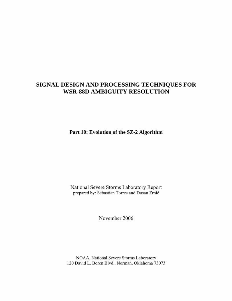
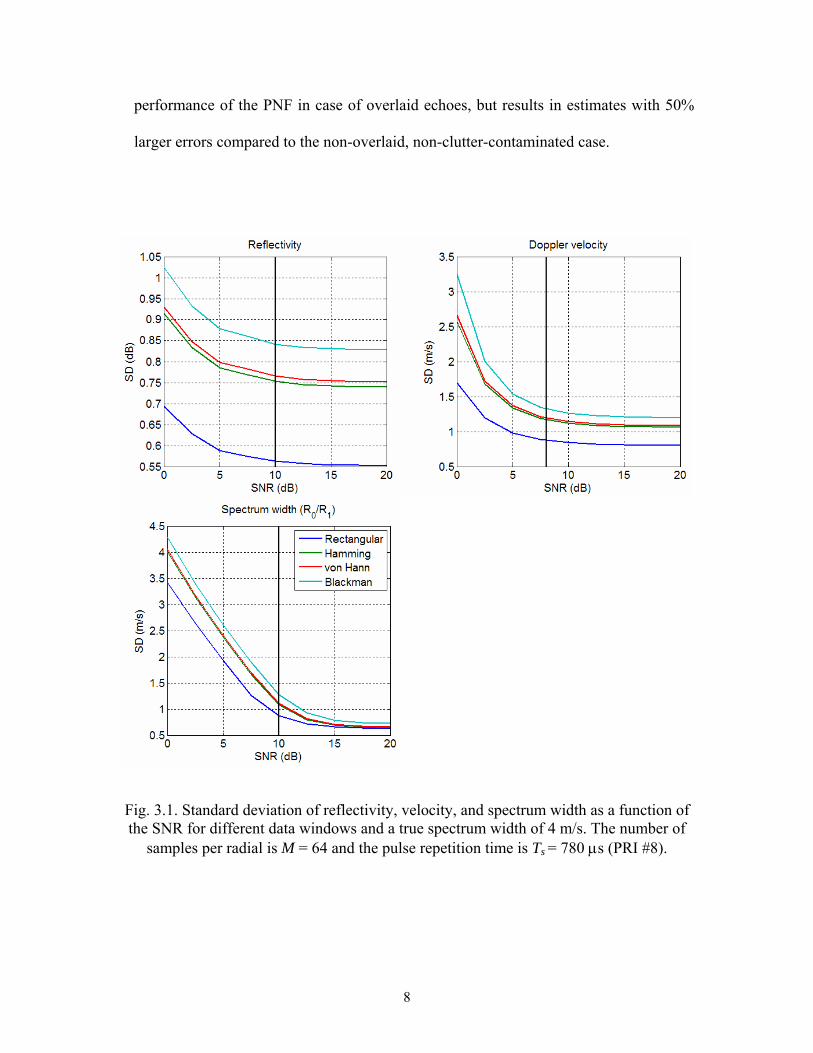
samples, and the higher are the errors of estimates. Fig. 3.1 shows the standard deviation

of spectral moment estimates as a function of the signal-to-noise ratio (SNR) for different

data windows, a true spectrum width of 4 m/s, and the parameters of VCP 211. For

example, compared to using a rectangular window, velocity errors for a spectrum width

of 4 m/s are about 33% higher with the Hamming window, 35% higher with the von

Hann window, and 50% higher with the Blackman window. In addition, it is evident from

this figure that NEXRAD technical requirements are not met with any data window other

than rectangular, because the standard deviation for high SNR is greater than the required

1 m/s.

With this in mind, we revisited the use of data windows in SZ-2 and recommended the

following use:

• The rectangular window should be use if there are no overlaid echoes or clutter

contamination. This results in the best statistical performance that matches the one in

the legacy RDA.

• The von Hann window should be used if there are overlaid echoes but no clutter

contamination. This results in an acceptable performance of the processing notch filter

(PNF) that is used to recover the weaker overlaid trip and an optimum statistical

performance for the overall algorithm. Note that errors of estimates recovered from

overlaid echoes are about 30% higher than those from non-overlaid echoes.

• The Blackman window should be used if there is clutter contamination (regardless of

the overlaid situation). This provides the required clutter suppression, acceptable

7

performance of the PNF in case of overlaid echoes, but results in estimates with 50%

larger errors compared to the non-overlaid, non-clutter-contaminated case.

Fig. 3.1. Standard deviation of reflectivity, velocity, and spectrum width as a function of the SNR for different data windows and a true spectrum width of 4 m/s. The number of

samples per radial is M = 64 and the pulse repetition time is Ts = 780 μs (PRI #8).

8

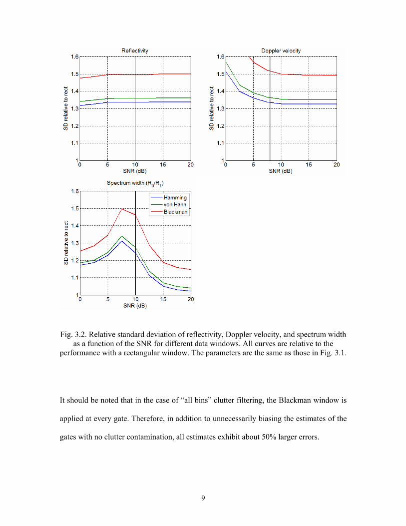
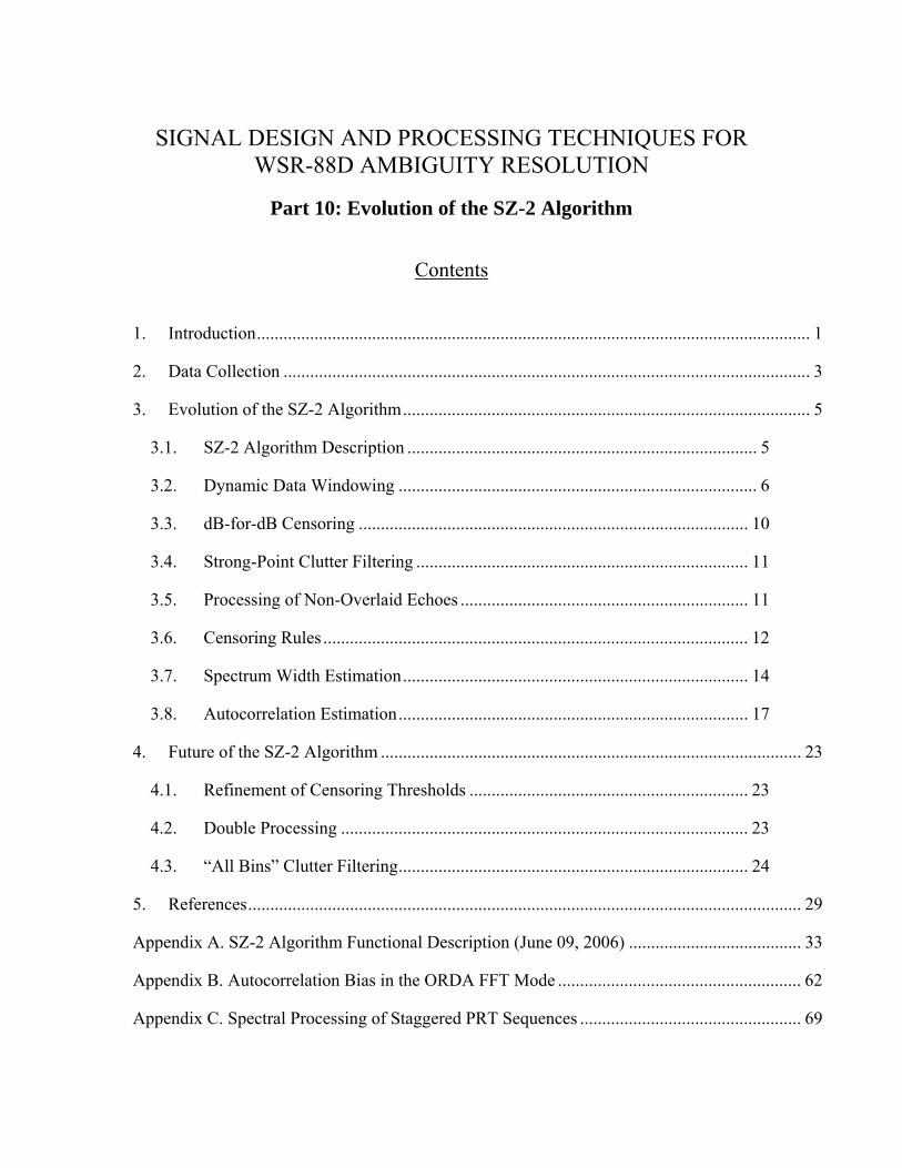
Fig. 3.2. Relative standard deviation of reflectivity, Doppler velocity, and spectrum width as a function of the SNR for different data windows. All curves are relative to the

performance with a rectangular window. The parameters are the same as those in Fig. 3.1.

It should be noted that in the case of “all bins” clutter filtering, the Blackman window is

applied at every gate. Therefore, in addition to unnecessarily biasing the estimates of the

gates with no clutter contamination, all estimates exhibit about 50% larger errors.

9

The operational version of the SZ-2 algorithm uses the “default” window for the non-

overlaid, non-clutter-contamination case. In the current version of the ORDA this is the

Hamming window. We recommend that the ROC reconfigures the ORDA system to use

the rectangular window as the default window in this and other cases. By not using a

tapered data window when it is not required, base data moment estimates will exhibit

about 30% less errors, bringing the ORDA system to par with the legacy RDA system.

Table 3.1 summarizes the effect of data windows on the statistical performance of

spectral moment estimators for the conditions specified in the NEXRAD technical

requirements (NTR) and the parameters of VCP 211. Note that only the rectangular

window leads to estimates that meet NTR requirements.

Rectangular Hamming von Hann Blackman

SD(Z) (dB) 0.57 0.76 0.77 0.85

SD(v) (m/s) 0.87 1.17 1.19 1.33

SD(σv) (m/s) 0.86 1.08 1.10 1.27

Table 3.1. Standard deviation of spectral moments for different data windows for the conditions specified in the NEXRAD technical requirements and the parameters of

VCP 211.

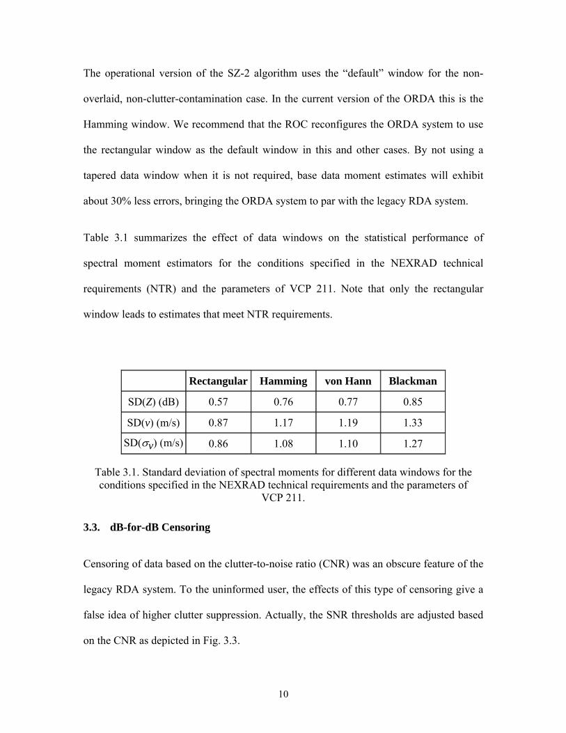
3.3. dB-for-dB Censoring

Censoring of data based on the clutter-to-noise ratio (CNR) was an obscure feature of the

legacy RDA system. To the uninformed user, the effects of this type of censoring give a

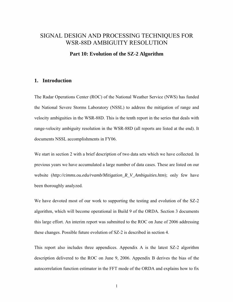
false idea of higher clutter suppression. Actually, the SNR thresholds are adjusted based

on the CNR as depicted in Fig. 3.3.

10

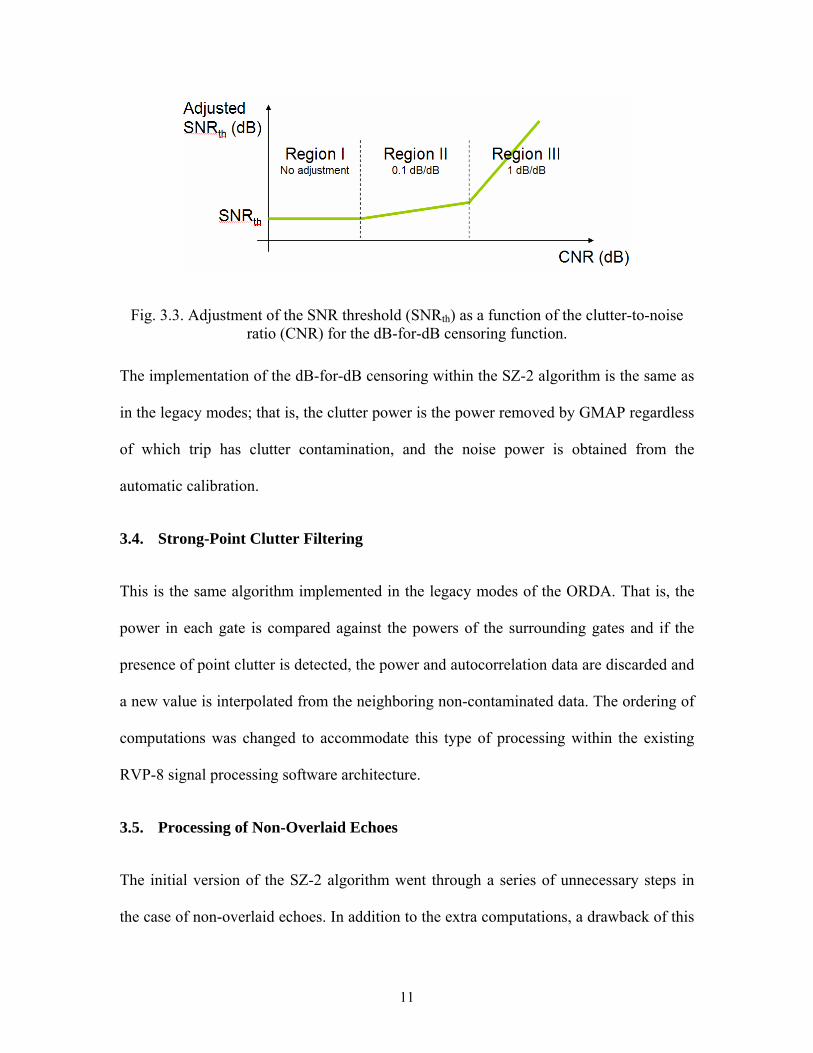
Fig. 3.3. Adjustment of the SNR threshold (SNRth) as a function of the clutter-to-noise ratio (CNR) for the dB-for-dB censoring function.

The implementation of the dB-for-dB censoring within the SZ-2 algorithm is the same as

in the legacy modes; that is, the clutter power is the power removed by GMAP regardless

of which trip has clutter contamination, and the noise power is obtained from the

automatic calibration.

3.4. Strong-Point Clutter Filtering

This is the same algorithm implemented in the legacy modes of the ORDA. That is, the

power in each gate is compared against the powers of the surrounding gates and if the

presence of point clutter is detected, the power and autocorrelation data are discarded and

a new value is interpolated from the neighboring non-contaminated data. The ordering of

computations was changed to accommodate this type of processing within the existing

RVP-8 signal processing software architecture.

3.5. Processing of Non-Overlaid Echoes

The initial version of the SZ-2 algorithm went through a series of unnecessary steps in

the case of non-overlaid echoes. In addition to the extra computations, a drawback of this

11

implementation is that the strong-trip residue after the PNF (i.e., the residue of the only

significant trip) acts as out-of-trip power, which biases the estimated signal power and the

corresponding spectrum width if using the R0/R1 estimator. The logic of the newly

recommended SZ-2 algorithm was modified so that the processing of non-overlaid

echoes is streamlined, resulting in a processing pipeline very similar to the one of the

legacy modes.

3.6. Censoring Rules

Due to the complexity of the SZ-2 algorithm, moment data must be censored based on

many more criteria than there are in the legacy modes. In addition, it is not obvious to

determine if censored data should be tagged as a noise-like return (black) or as an

overlaid-like return (purple). After the initial evaluation of the SZ-2 algorithm, it was

established that the behavior of the SZ-2 algorithm in terms of censoring was different

than it was expected. That is, gates that should be “black” were shown as “purple” and

vice versa. The underlying problem was a lack of a clear definition of the censoring

classes. For example, significant but unrecoverable data should be purple, but data

censored via the dB-for-dB censoring algorithm is routinely tagged as noise-like (and this

is the expected behavior of the system). It was obvious that, in addition to maintain

expected system behavior, we needed a clear set of rules that we could convey to users to

help them understand the specific behavior of the SZ-2 algorithm.

12

In the SZ-2 algorithm gates are classified as follows:

• Signal-like return: a gate with signal power above the dB-for-dB adjusted SNR

threshold that is recoverable (i.e., it passes all tests).

• Noise-like return: a gate with signal power below the SNR threshold or with signal

power below the dB-for-dB adjusted SNR threshold in the non-overlaid case.

• Overlaid-like return: a gate with signal power above the SNR threshold in the overlaid

case that is unrecoverable (i.e., at least one test fails).

Censoring rules are summarized in Tables 3.2, 3.3, and 3.4 for the strong trip, weak trip,

and other trips, respectively.

Rule Threshold Class Notes

SNR long PRT KSNR,V NOISE

SNR short PRT KSNR,V NOISE

NOISE Non-overlaid echoesCNR short PRT adjusted KSNR,V

OVERLAID Overlaid Echoes

NOISE Non-overlaid echoesCSR long PRT KCSR1

OVERLAID Overlaid Echoes

SNR* KS OVERLAID

Table 3.2. Censoring rules for the strong trip.

13

Rule Threshold Class Notes

SNR long PRT KSNR,V NOISE

SNR short PRT KSNR,V NOISE

CNR short PRT adjusted KSNR OVERLAID

CSR long PRT KCSR2 OVERLAID

SNR* KW OVERLAID

Recovery region Kr=f(wS,ww,CT,CS,CI) OVERLAID

Clutter location OVERLAID

Width long PRT Wmax OVERLAID Censoring applies to spectrum width

only

Table 3.3. Censoring rules for the weak trip.

Rule Threshold Class Notes

NOISE Non-significant return SNR long PRT KSNR,V

OVERLAID Significant return

Table 3.4. Censoring rules for the other trips.

3.7. Spectrum Width Estimation

The two most commonly used time-domain spectrum width estimators are the one based

on the lag-0 to the lag-1 autocorrelation magnitude ratio (herein referred to as the R0/R1

estimator) and the one based on the lag-1 to the lag-2 autocorrelation magnitude ratio

(herein referred to as the R1/R2 estimator). On one hand, the R0/R1 estimator has a wider

usable range but requires precise knowledge of the signal and noise powers. This makes

14

it a bad candidate for low SNR situations and in the presence of overlaid echoes because

it is more difficult to precisely determine each of the overlaid powers. On the other hand,

the R1/R2 estimator does not require either the signal or the noise powers, which makes it

a good candidate for situations with low SNR or overlaid echoes. However, this estimator

has a limited usable range (about half of the R0/R1 estimator). The initial version of the

SZ-2 algorithm used solely the R0/R1 estimator to match the behavior of the legacy RDA

system. Ideally, we would like to have an adaptive scheme to select the best spectrum

width estimator for each situation. However, this is difficult in practice since the best

estimator depends on the actual spectrum width! A simple compromise is to use the

R1/R2 estimator with overlaid echoes and the R0/R1 estimator otherwise (similar

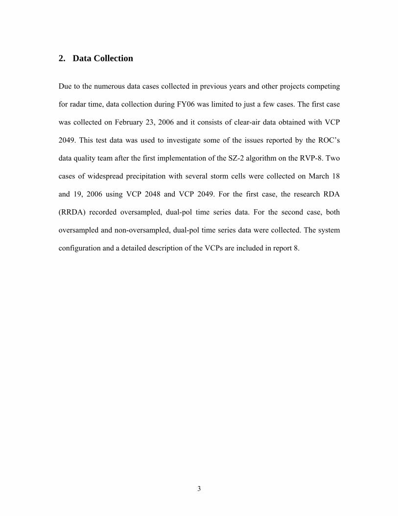
behavior to the legacy RDA). Figure 3.4 shows the spectrum width fields computed with

the R0/R1 and R1/R2 estimators. The properties of each estimator are evident when

comparing these two figures.

15

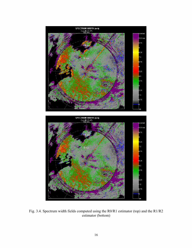
Fig. 3.4. Spectrum width fields computed using the R0/R1 estimator (top) and the R1/R2 estimator (bottom)

16

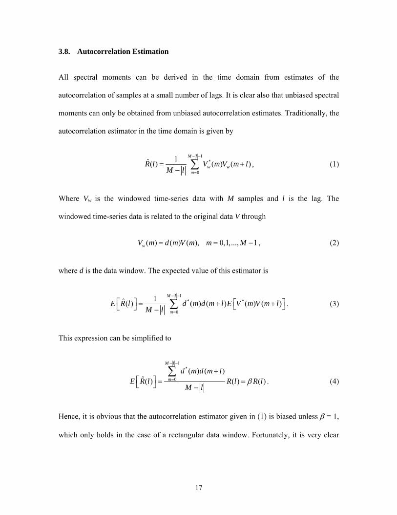
3.8. Autocorrelation Estimation

All spectral moments can be derived in the time domain from estimates of the

autocorrelation of samples at a small number of lags. It is clear also that unbiased spectral

moments can only be obtained from unbiased autocorrelation estimates. Traditionally, the

autocorrelation estimator in the time domain is given by

1

*

0

1ˆ( ) ( ) ( )− −

=

=− ∑

M l

w wm

+R l V m VM l

m l

−

, (1)

Where Vw is the windowed time-series data with M samples and l is the lag. The

windowed time-series data is related to the original data V through

, (2) ( ) ( ) ( ), 0,1,..., 1= =wV m d m V m m M

where d is the data window. The expected value of this estimator is

1

* *

0

1ˆ( ) ( ) ( ) ( ) ( )− −

=

⎡ ⎤ ⎡ ⎤= + +⎣ ⎦⎣ ⎦ − ∑M l

mE R l d m d m l E V m V m l

M l. (3)

This expression can be simplified to

1*

0

( ) ( )ˆ( ) ( ) ( )β

− −

=

+⎡ ⎤ =⎣ ⎦ −

∑M l

m

d m d m lE R l R l R l

M l= . (4)

Hence, it is obvious that the autocorrelation estimator given in (1) is biased unless β = 1,

which only holds in the case of a rectangular data window. Fortunately, it is very clear

17

from (4) how to unbias it. An unbiased estimator of the autocorrelation function for any

data window is given by

1*

01

*

0

( ) ( )ˆ( )

( ) ( )

− −

=− −

=

+=

+

∑

∑

M l

w wm

M l

m

V m V m lR l

d m d m l. (5)

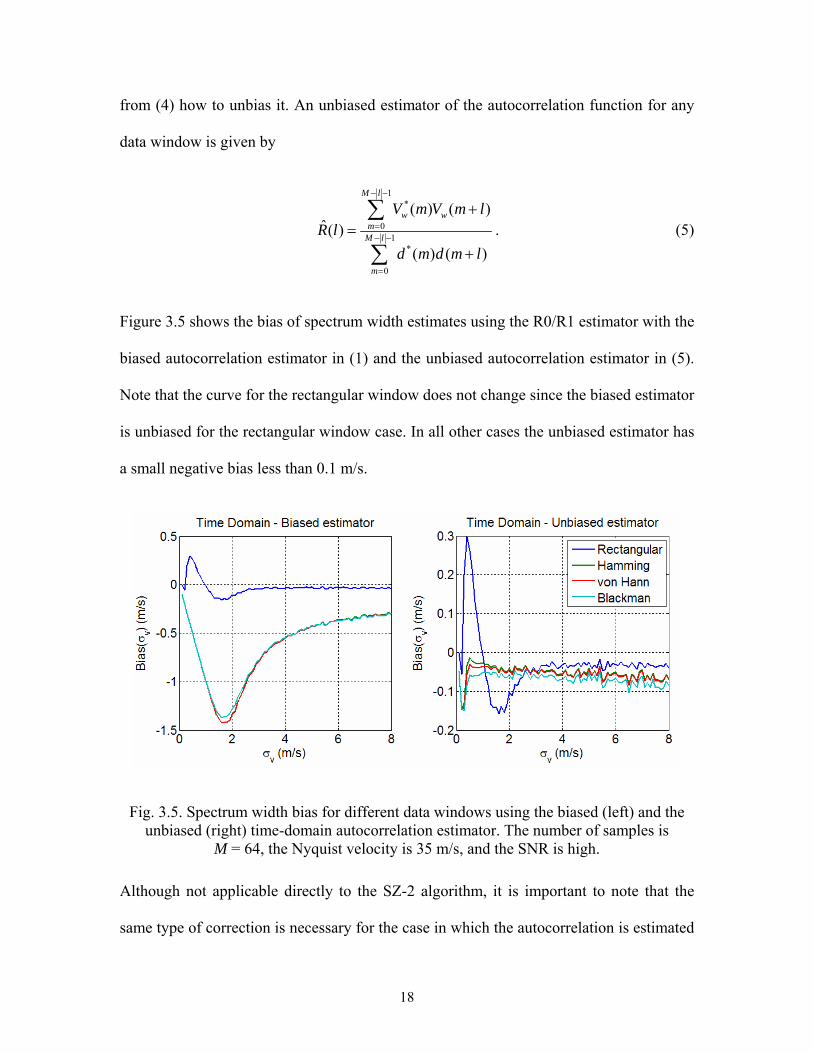
Figure 3.5 shows the bias of spectrum width estimates using the R0/R1 estimator with the

biased autocorrelation estimator in (1) and the unbiased autocorrelation estimator in (5).

Note that the curve for the rectangular window does not change since the biased estimator

is unbiased for the rectangular window case. In all other cases the unbiased estimator has

a small negative bias less than 0.1 m/s.

Fig. 3.5. Spectrum width bias for different data windows using the biased (left) and the unbiased (right) time-domain autocorrelation estimator. The number of samples is

M = 64, the Nyquist velocity is 35 m/s, and the SNR is high.

Although not applicable directly to the SZ-2 algorithm, it is important to note that the

same type of correction is necessary for the case in which the autocorrelation is estimated

18

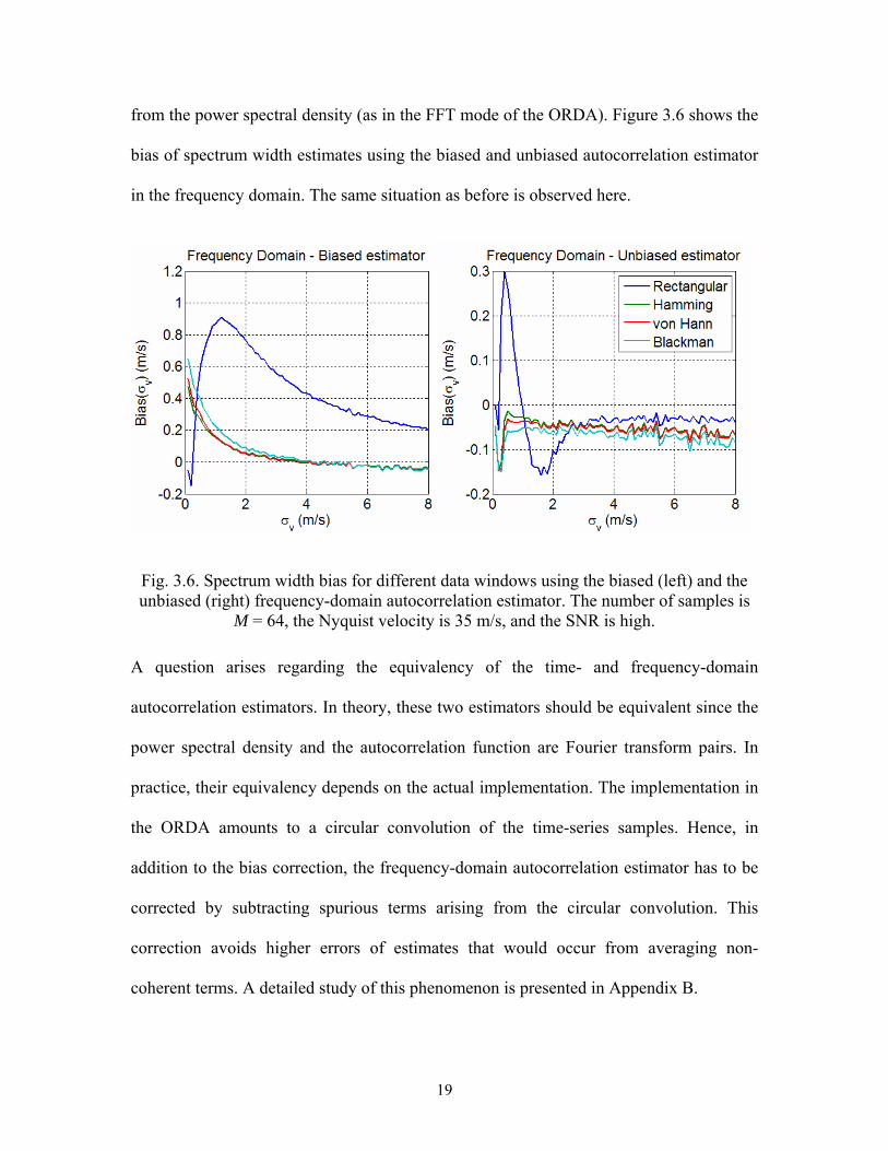
from the power spectral density (as in the FFT mode of the ORDA). Figure 3.6 shows the

bias of spectrum width estimates using the biased and unbiased autocorrelation estimator

in the frequency domain. The same situation as before is observed here.

Fig. 3.6. Spectrum width bias for different data windows using the biased (left) and the unbiased (right) frequency-domain autocorrelation estimator. The number of samples is

M = 64, the Nyquist velocity is 35 m/s, and the SNR is high.

A question arises regarding the equivalency of the time- and frequency-domain

autocorrelation estimators. In theory, these two estimators should be equivalent since the

power spectral density and the autocorrelation function are Fourier transform pairs. In

practice, their equivalency depends on the actual implementation. The implementation in

the ORDA amounts to a circular convolution of the time-series samples. Hence, in

addition to the bias correction, the frequency-domain autocorrelation estimator has to be

corrected by subtracting spurious terms arising from the circular convolution. This

correction avoids higher errors of estimates that would occur from averaging non-

coherent terms. A detailed study of this phenomenon is presented in Appendix B.

19

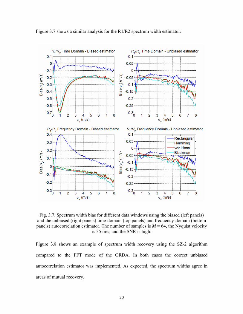
Figure 3.7 shows a similar analysis for the R1/R2 spectrum width estimator.

Fig. 3.7. Spectrum width bias for different data windows using the biased (left panels) and the unbiased (right panels) time-domain (top panels) and frequency-domain (bottom panels) autocorrelation estimator. The number of samples is M = 64, the Nyquist velocity

is 35 m/s, and the SNR is high.

Figure 3.8 shows an example of spectrum width recovery using the SZ-2 algorithm

compared to the FFT mode of the ORDA. In both cases the correct unbiased

autocorrelation estimator was implemented. As expected, the spectrum widths agree in

areas of mutual recovery.

20

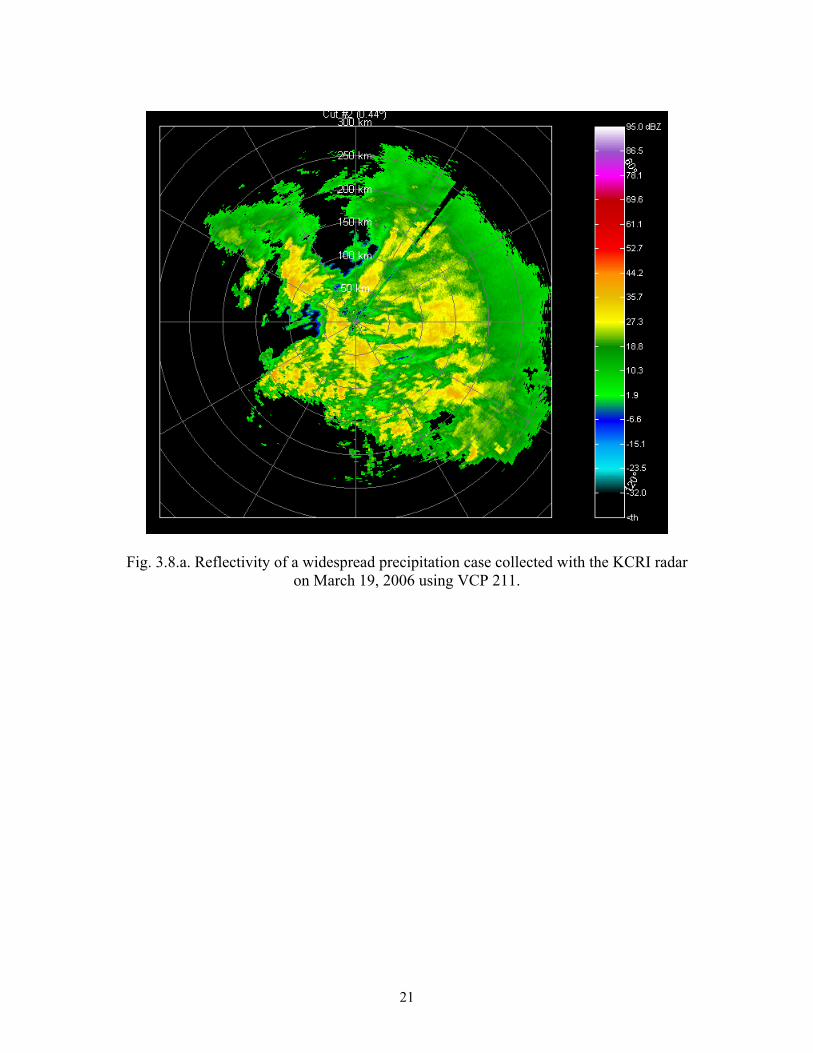
Fig. 3.8.a. Reflectivity of a widespread precipitation case collected with the KCRI radar on March 19, 2006 using VCP 211.

21

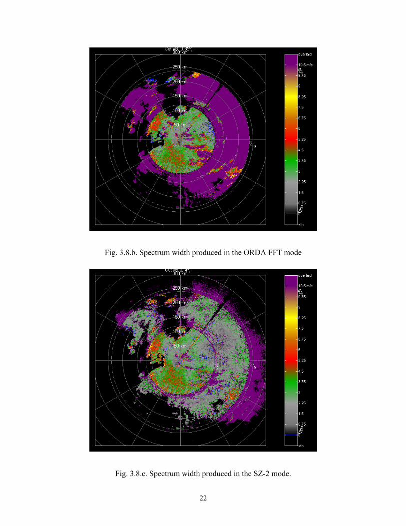
Fig. 3.8.b. Spectrum width produced in the ORDA FFT mode

Fig. 3.8.c. Spectrum width produced in the SZ-2 mode.

22

4. Future of

orithm marks the completion of the first

to the SZ-2 algorithm. These have been

covery of the strong-trip velocity is more difficult if the strong

the SZ-2 Algorithm

The operational implementation of the SZ-2 alg

stage of range and velocity ambiguity mitigation for the NEXRAD network. The

performance of the recommended algorithm has been tested using numerous cases and

has been deemed acceptable for the operational community. However, there is room for

improvement in at least three areas which we discuss next.

4.1. Refinement of Censoring Thresholds

There are currently 14 thresholds specific

established empirically after analyzing a limited number of cases. A more detail study

that employs data collected under varied weather situations could result in further

refinement of these thresholds. It is always recommended to censor on the conservative

side to avoid feeding bad-quality data to the users and algorithms. However, a balance

needs to be found to avoid censoring of valid and useful data.

4.2. Double Processing

It has been observed that re

and weak trip powers are about the same. This is because the strong trip velocity is

recovered directly, without attempting to remove contamination from the out-of-trip

echoes (report 9). Recovery of the weak-trip velocity is not affected by this because the

weak-trip velocity is always recovered after notching most of the strong-trip echo with

the “processing notch filter” (PNF). Thus, if the strong and weak trip powers are about

the same, we could recover the strong trip velocity in a similar way as we do the weak

23

trip velocity; i.e., by means of a PNF. This is termed as double processing and was

discussed in detail in our previous report. To summarize, double processing for SZ-2

improves the recovery of the strong-trip velocity for strong-to-weak power ratios less

than at least 3 dB and the usual range of spectrum width values. It is obvious that double

processing, as its name implies, would almost double the computational complexity of

the SZ-2 algorithm. Hence, its benefits will have to be weighed against the required

additional computational power (if available). As part of future work we plan to

investigate the performance of double processing in the presence of clutter and using

adaptive PNF notch widths for both the strong and weak-trip PNFs.

4.3. “All Bins” Clutter Filtering

It was demonstrated that the current SZ-2 algorithm cannot recover overlaid signals if

multiple trips have clutter contamination (herein referred to as “overlaid clutter”). Faced

with this situation, the algorithm will tag all trips with significant returns as overlaid-like.

If the operator selects clutter filtering in all bins, this forces the occurrence of overlaid

clutter in every gate which results in a significant increase of “purple haze”. However,

even if the bypass map commands filtering everywhere, not all bins have clutter

contamination. Knowing exactly which bins have clutter contamination is a difficult

problem that is currently being addressed by other algorithms under research (e.g.,

NCAR’s Clutter Mitigation Decision or CMD). A simple way to determine the presence

of clutter in a given gate is to use GMAP as a proxy. Since GMAP already employs a

“smart” algorithm to decide how much clutter power to remove from the power spectrum,

the power removed by GMAP can be used as an indicator of clutter presence. Using the

clutter-to-signal ratio (CSR) from the long-PRT scan was recommended in the current

24

version of the SZ-2 algorithm as a way to avoid large amounts of “purple haze” in the all-

bins situation (note that the use of the CSR only applies when the bypass map indicates

the presence of overlaid clutter as a way to re-determine the presence of clutter). The

CSR is computed as the ratio of the power removed by GMAP to the remaining power

after filtering. The scheme is simple and works well most of the time. However, it was

determined that the recommended test fails sometimes by incorrectly identifying a gate as

not having clutter contamination, therefore producing biased estimates of all moments. A

way to mitigate this problem is to use the long-PRT clutter-to-noise ratio (CNR), which

only uses one parameter provided by GMAP. As shown in Fig. 3.9, preliminary tests

confirm that this seems to minimize the occurrence of false negatives.

Fig. 3.9.a. Doppler velocity field with a proper clutter map.

25

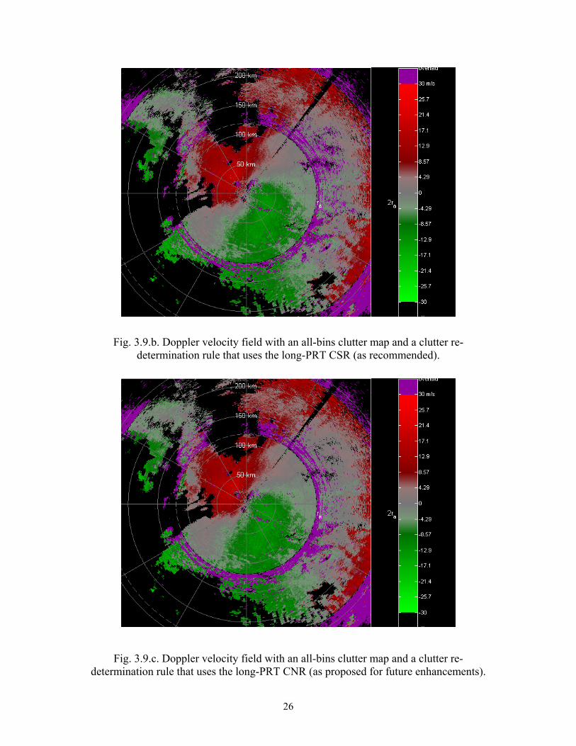
Fig. 3.9.b. Doppler velocity field with an all-bins clutter map and a clutter re-determination rule that uses the long-PRT CSR (as recommended).

determination rule that uses the long-PRT CNR (as proposed for future enhancements).

Fig. 3.9.c. Doppler velocity field with an all-bins clutter map and a clutter re-

26

27

5. References

Ice, R. L., D. A. Warde, D. Sirmans, and D. Rachel, 2004: Open RDA – RVP8 Signal Processing. Part 1: Simulation Study, WSR-88D Radar Operations Center Report, 87 pp.

Sachidananda, M., D. Zrnić, and R. Doviak, 1998: Signal design and processing techniques for WSR-88D ambiguity resolution, NOAA/NSSL Report, Part 2, 105 pp.

Torres S., M. Sachidananda, and D. Zrnić, 2004: Signal Design and Processing Techniques for WSR-88D Ambiguity Resolution: Phase coding and staggered PRT: Data collection, implementation, and clutter filtering, NOAA/NSSL Report, Part 8, 113 pp.

Torres S., M. Sachidananda, and D. Zrnić, 2005: Signal Design and Processing Techniques for WSR-88D Ambiguity Resolution, NOAA/NSSL Report, Part 9, 112 pp.

29

30

LIST OF NSSL REPORTS FOCUSED ON POSSIBLE UPGRADES

TO THE WSR-88D RADARS

Torres S., M. Sachidananda, and D. Zrnić, 2005: Signal Design and Processing Techniques for WSR-88D Ambiguity Resolution: Phase coding and staggered PRT. NOAA/NSSL Report, Part 9, 112 pp.

Zrnić, D.S., Melnikov, V.M., and J.K. Carter, 2005: Calibrating differential reflectivity on the WSR-88D. NOAA/NSSL Report, 34 pp.

Torres S., M. Sachidananda, and D. Zrnić, 2004: Signal Design and Processing Techniques for WSR-88D Ambiguity Resolution: Phase coding and staggered PRT: Data collection, implementation, and clutter filtering. NOAA/NSSL Report, Part 8, 113 pp.

Zrnić, D., S. Torres, J. Hubbert, M. Dixon, G. Meymaris, and S. Ellis, 2004: NEXRAD range-velocity ambiguity mitigation. SZ-2 algorithm recommendations. NCAR-NSSL Interim Report.

Melnikov, V, and D Zrnić, 2004: Simultaneous transmission mode for the polarimetric WSR-88D – statistical biases and standard deviations of polarimetric variables. NOAA/NSSL Report, 84 pp.

Bachman, S., 2004: Analysis of Doppler spectra obtained with WSR-88D radar from non-stormy environment. NOAA/NSSL Report, 86 pp.

Zrnić, D., S. Torres, Y. Dubel, J. Keeler, J. Hubbert, M. Dixon, G. Meymaris, and S. Ellis, 2003: NEXRAD range-velocity ambiguity mitigation. SZ(8/64) phase coding algorithm recommendations. NCAR-NSSL Interim Report.

Torres S., D. Zrnić, and Y. Dubel, 2003: Signal Design and Processing Techniques for WSR-88D Ambiguity Resolution: Phase coding and staggered PRT: Implementation, data collection, and processing. NOAA/NSSL Report, Part 7, 128 pp.

Schuur, T., P. Heinselman, and K. Scharfenberg, 2003: Overview of the Joint Polarization Experiment (JPOLE), NOAA/NSSL Report, 38 pp.

Ryzhkov, A, 2003: Rainfall Measurements with the Polarimetric WSR-88D Radar, NOAA/NSSL Report, 99 pp.

Schuur, T., A. Ryzhkov, and P. Heinselman, 2003: Observations and Classification of echoes with the Polarimetric WSR-88D radar, NOAA/NSSL Report, 45 pp.

Melnikov, V., D. Zrnić, R. J. Doviak, and J. K. Carter, 2003: Calibration and Performance Analysis of NSSL’s Polarimetric WSR-88D, NOAA/NSSL Report, 77 pp.

31

NCAR-NSSL Interim Report, 2003: NEXRAD Range-Velocity Ambiguity Mitigation SZ(8/64) Phase Coding Algorithm Recommendations.

Sachidananda, M., 2002: Signal Design and Processing Techniques for WSR-88D Ambiguity Resolution, NOAA/NSSL Report, Part 6, 57 pp.

Doviak, R., J. Carter, V. Melnikov, and D. Zrnić, 2002: Modifications to the Research WSR-88D to obtain Polarimetric Data, NOAA/NSSL Report, 49 pp.

Fang, M., and R. Doviak, 2001: Spectrum width statistics of various weather phenomena, NOAA/NSSL Report, 62 pp.

Sachidananda, M., 2001: Signal Design and Processing Techniques for WSR-88D Ambiguity Resolution, NOAA/NSSL Report, Part 5, 75 pp.

Sachidananda, M., 2000: Signal Design and Processing Techniques for WSR-88D Ambiguity Resolution, NOAA/NSSL Report, Part 4, 99 pp.

Sachidananda, M., 1999: Signal Design and Processing Techniques for WSR-88D Ambiguity Resolution, NOAA/NSSL Report, Part 3, 81 pp.

Sachidananda, M., 1998: Signal Design and Processing Techniques for WSR-88D Ambiguity Resolution, NOAA/NSSL Report, Part 2, 105 pp.

Torres, S., 1998: Ground Clutter Canceling with a Regression Filter, NOAA/NSSL Report, 37 pp.

Doviak, R. and D. Zrnić, 1998: WSR-88D Radar for Research and Enhancement of Operations: Polarimetric Upgrades to Improve Rainfall Measurements, NOAA/NSSL Report, 110 pp.

Sachidananda, M., 1997: Signal Design and Processing Techniques for WSR-88D Ambiguity Resolution, NOAA/NSSL Report, Part 1, 100 pp.

Sirmans, D., D. Zrnić, and M. Sachidananda, 1986: Doppler radar dual polarization considerations for NEXRAD, NOAA/NSSL Report, Part I, 109 pp.

Sirmans, D., D. Zrnić, and N. Balakrishnan, 1986: Doppler radar dual polarization considerations for NEXRAD, NOAA/NSSL Report, Part II, 70 pp.

32

Appendix A. SZ-2 Algorithm Functional Description (June 09, 2006)

A.1. Introduction

This appendix reproduces the latest recommended SZ-2 algorithm as reported in the

FY2006 NCAR-NSSL Interim Report, “NEXRAD Range-Velocity Ambiguity Mitigation

SZ(8/64) Phase Coding Algorithm Recommendations”, 09 June, 2006. The SZ-2

algorithm herein described has been updated and includes modifications to use dynamic

windows, unbiased spectrum width computations, and efficient processing of non-

overlaid echoes.

To facilitate the programming of these changes, the recommended SZ-2 code builds on

the existing real-time implementation by the ROC. In addition, the latest revision brings

the algorithm description much closer to the actual RVP-8 implementation.

When implemented on the NEXRAD ORDA the recommended SZ-2 algorithm will

significantly outperform the legacy range-velocity mitigation algorithm. However, the

SZ-2 algorithm is still in its infancy and needs to be tested on much more experimental

data. Further refinements can and should be made to obtain the best data quality and to

minimize the amount of censored data.

A.2. SZ-2 Algorithm Description

The SZ-2 algorithm was first introduced by Sachidananda et al. (1998) in a study of range

and velocity ambiguity mitigation using phase coding. Unlike the stand-alone SZ-1

algorithm, SZ-2 relies on power and spectrum width estimates obtained using a long

pulse repetition time (PRT). The SZ-2 algorithm is computationally simpler than its

33

stand-alone counterpart as it only tries to recover the Doppler velocities associated with

strong- and weak-trip signals and the spectrum widths associated with the strong-trip

signal. Analogous to the legacy “split cut”, the volume coverage pattern (VCP) is

designed such that a non-phase-coded scan using a long PRT is immediately followed by

a scan with phase-coded signals using a short PRT at the same elevation angle. Hence,

determination of the number and location of overlaid trips can be done by examining the

overlay-free long-PRT powers.

The following is a functional description of the SZ-2 algorithm tailored for insertion into

the signal processing pipeline of the RVP-8. The description is divided into two parts:

long PRT processing and short PRT processing with emphasis given to the latter. The

algorithm is specified in a general manner and is not constrained to specific PRT values.

34

A.3. Long-PRT Processing

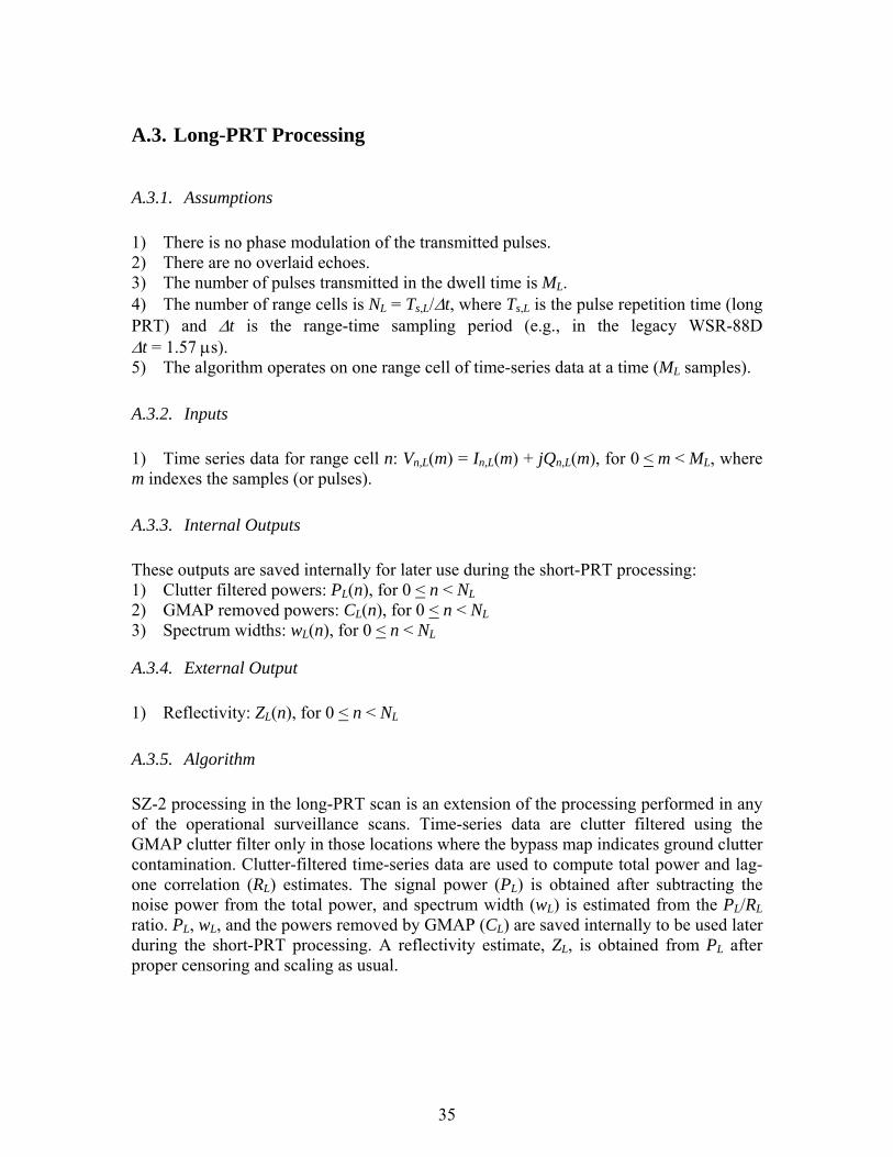
A.3.1. Assumptions

1) There is no phase modulation of the transmitted pulses. 2) There are no overlaid echoes. 3) The number of pulses transmitted in the dwell time is ML. 4) The number of range cells is NL = Ts,L/Δt, where Ts,L is the pulse repetition time (long PRT) and Δt is the range-time sampling period (e.g., in the legacy WSR-88D Δt = 1.57 μs). 5) The algorithm operates on one range cell of time-series data at a time (ML samples).

A.3.2. Inputs

1) Time series data for range cell n: Vn,L(m) = In,L(m) + jQn,L(m), for 0 < m < ML, where m indexes the samples (or pulses).

A.3.3. Internal Outputs

These outputs are saved internally for later use during the short-PRT processing: 1) Clutter filtered powers: PL(n), for 0 < n < NL 2) GMAP removed powers: CL(n), for 0 < n < NL 3) Spectrum widths: wL(n), for 0 < n < NL

A.3.4. External Output

1) Reflectivity: ZL(n), for 0 < n < NL

A.3.5. Algorithm

SZ-2 processing in the long-PRT scan is an extension of the processing performed in any of the operational surveillance scans. Time-series data are clutter filtered using the GMAP clutter filter only in those locations where the bypass map indicates ground clutter contamination. Clutter-filtered time-series data are used to compute total power and lag-one correlation (RL) estimates. The signal power (PL) is obtained after subtracting the noise power from the total power, and spectrum width (wL) is estimated from the PL/RL ratio. PL, wL, and the powers removed by GMAP (CL) are saved internally to be used later during the short-PRT processing. A reflectivity estimate, ZL, is obtained from PL after proper censoring and scaling as usual.

35

A.4. Short-PRT Processing

A.4.1. Assumptions

1) The phases of the transmitted pulses are modulated with the SZ(8/64) switching code. 2) Regardless of the number of pulses transmitted in the dwell time M = 64 pulses worth of data are supplied to the algorithm. 3) The number of range cells is N = Ts/Δt, where Ts is the pulse repetition time (short PRT) and Δt is the range-time sampling period (e.g., in the legacy WSR-88D Δt = 1.57 μs). 4) Range cells in the short-PRT scan are perfectly aligned with range cells in the long-PRT scan. This is important for determining short-PRT trips within the long-PRT data. Note: Misalignments may occur, for example, due to Ts/Δt not being an integer number or due to one or more samples being dropped. 5) Long- and short-PRT radials are perfectly aligned in azimuth. This is true for the ORDA system, which collects data on indexed radials. 6) The algorithm operates on one range cell (M samples) of time-series data at a time, but requires all cells to perform strong-point clutter suppression.

A.4.2. Inputs

1) Phase-coded time series data cohered to the 1st trip: Vn(m) = In(m) + jQn(m), for 0 < m < M, where m indexes the samples (or pulses) and n indexes the range gates. 2) Ground-clutter-filtered powers and spectrum widths from the long-PRT scan: PL and wL. These vectors correspond to the long-PRT scan radial that has the same (or closest) azimuth to the phase-coded radial in (1). 3) GMAP removed powers: CL. This vector corresponds to the long-PRT scan radial that has the same (or closest) azimuth to the phase-coded radial in (1). 4) Range-dependent ground clutter filter bypass map corresponding to the long- and short-PRT radials (B). B can be either FILTER or BYPASS, indicating the presence or absence of clutter, respectively.

( )m5) Measured SZ(8/64) switching code: ψ , for −3 < m < M. 6) Censoring thresholds:

KSNR,Z: signal-to-noise (SNR) threshold for determination of significant returns for reflectivity, KSNR,V: signal-to-noise (SNR) threshold for determination of significant returns for velocity, KIGN: power ratio threshold to ignore trips with small total powers, Ks: signal-to-noise ratio (SNR) threshold for determination of strong trip recovery, Kw: signal-to-noise ratio (SNR) threshold for determination of weak trip recovery, Kr(wSn, wWn): maximum strong-to-weak power ratios (PS/PW) for recovery of the weaker trip for different values of strong- and weak-trip normalized spectrum widths

36

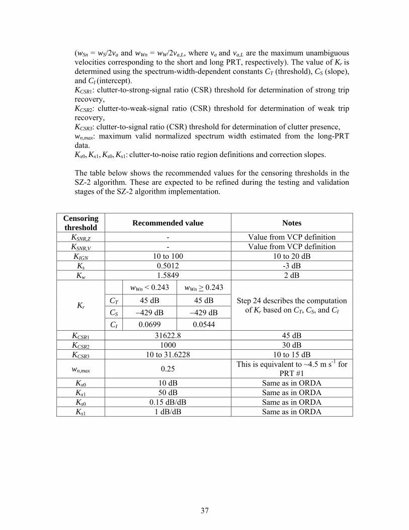
(wSn = wS/2va and wWn = wW/2va,L, where va and va,L are the maximum unambiguous velocities corresponding to the short and long PRT, respectively). The value of Kr is determined using the spectrum-width-dependent constants CT (threshold), CS (slope), and CI (intercept). KCSR1: clutter-to-strong-signal ratio (CSR) threshold for determination of strong trip recovery, KCSR2: clutter-to-weak-signal ratio (CSR) threshold for determination of weak trip recovery, KCSR3: clutter-to-signal ratio (CSR) threshold for determination of clutter presence, wn,max: maximum valid normalized spectrum width estimated from the long-PRT data. Kx0, Kx1, Ks0, Ks1: clutter-to-noise ratio region definitions and correction slopes. The table below shows the recommended values for the censoring thresholds in the SZ-2 algorithm. These are expected to be refined during the testing and validation stages of the SZ-2 algorithm implementation.

Censoring threshold Recommended value Notes

KSNR,Z - Value from VCP definition KSNR,V - Value from VCP definition KIGN 10 to 100 10 to 20 dB Ks 0.5012 -3 dB Kw 1.5849 2 dB

wWn < 0.243 wWn > 0.243 CT 45 dB 45 dB CS −429 dB −429 dB

Kr

CI 0.0699 0.0544

Step 24 describes the computation of Kr based on CT, CS, and CI

KCSR1 31622.8 45 dB KCSR2 1000 30 dB KCSR3 10 to 31.6228 10 to 15 dB

wn,max 0.25 This is equivalent to ~4.5 m s-1 for PRT #1

Kx0 10 dB Same as in ORDA Kx1 50 dB Same as in ORDA Ks0 0.15 dB/dB Same as in ORDA Ks1 1 dB/dB Same as in ORDA

37

A.4.3. Outputs

1) Doppler velocities for 4 trips: ( ),0 4≤ <v n n N 2) Spectrum widths for 4 trips: ( ),0 4≤ <w n n N

( )type n( )type n 0 4≤ <n N

3) Return types for Doppler velocity and spectrum width for 4 trips: and

, . As in the legacy WSR-88D, type can take the values NOISE_LIKE, SIGNAL_LIKE, or OVERLAID_LIKE. These are used to qualify the base data moments sent to the RPG as being non-significant returns, significant returns, or unrecoverable overlaid echoes, respectively.

v

w

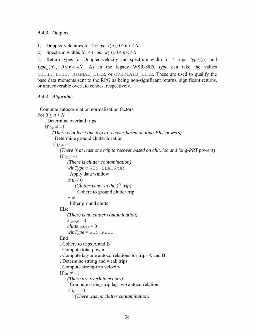
A.4.4. Algorithm

. Compute autocorrelation normalization factors For 0 < n < N . Determine overlaid trips If tAo ≠ −1 (There is at least one trip to recover based on long-PRT powers) . Determine ground clutter location If tA ≠ −1 (There is at least one trip to recover based on clut. loc and long-PRT powers) If tC ≠ −1 (There is clutter contamination) winType = WIN_BLACKMAN . Apply data window If tC ≠ 0 (Clutter is not in the 1st trip) . Cohere to ground clutter trip End . Filter ground clutter Else (There is no clutter contamination) kGMAP = 0 clutterGMAP = 0 winType = WIN_RECT End . Cohere to trips A and B . Compute total power . Compute lag-one autocorrelations for trips A and B . Determine strong and weak trips . Compute strong-trip velocity If tW ≠ −1 (There are overlaid echoes) . Compute strong-trip lag-two autocorrelation If tC = −1 (There was no clutter contamination)

38

winType = WIN_VONHANN . Apply data window End . Compute discrete Fourier transform . Apply processing notch filter . Compute inverse discrete Fourier transform . Compute weak-trip power . Cohere to weak trip . Compute weak-trip lag-one autocorrelation . Retrieve weak-trip spectrum width . Adjust powers . Compute strong-trip spectrum width using R1/R2 estimator Else (There are no overlaid echoes) . Adjust powers . Compute strong-trip spectrum width using R0/R1 estimator End Else (There are no trips to recover based on clutter location) clutterGMAP = 0 tS = tW = −1 End Else (There are no trips to recover based on long-PRT powers) clutterGMAP = 0 tS = tW = tC = −1 End . Compute SNR threshold adjustment factors . Determine censoring and moments End . Filter strong point clutter . Determine outputs

39

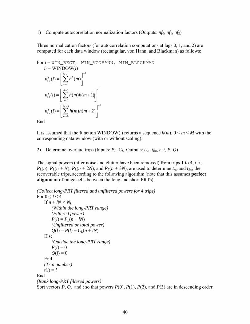
1) Compute autocorrelation normalization factors (Outputs: nf0, nf1, nf2)

Three normalization factors (for autocorrelation computations at lags 0, 1, and 2) are computed for each data window (rectangular, von Hann, and Blackman) as follows: For i = WIN_RECT, WIN_VONHANN, WIN_BLACKMAN h = WINDOW(i)

112

00

12

10

13

20

( ) ( )

( ) ( ) ( 1)

( ) ( ) ( 2)

−−

=

−−

=

−−

=

⎡ ⎤= ⎢ ⎥⎣ ⎦

⎡ ⎤= +⎢ ⎥⎣ ⎦

⎡ ⎤= +⎢ ⎥⎣ ⎦

∑

∑

∑

M

m

M

m

M

m

nf i h m

nf i h m h m

nf i h m h m

End It is assumed that the function WINDOW(.) returns a sequence h(m), 0 < m < M with the corresponding data window (with or without scaling). 2) Determine overlaid trips (Inputs: PL, CL. Outputs: tAo, tBo, r, t, P, Q)

The signal powers (after noise and clutter have been removed) from trips 1 to 4, i.e., PL(n), PL(n + N), PL(n + 2N), and PL(n + 3N), are used to determine tAo and tBo, the recoverable trips, according to the following algorithm (note that this assumes perfect alignment of range cells between the long and short PRTs). (Collect long-PRT filtered and unfiltered powers for 4 trips) For 0 < l < 4

If n + lN < NL

(Within the long-PRT range) (Filtered power) P(l) = PL(n + lN) (Unfiltered or total power)

Q(l) = P(l) + CL(n + lN) Else (Outside the long-PRT range) P(l) = 0 Q(l) = 0 End (Trip number) t(l) = l

End (Rank long-PRT filtered powers) Sort vectors P, Q, and t so that powers P(0), P(1), P(2), and P(3) are in descending order

40

with their corresponding total powers as Q(0), Q(1), Q(2), and Q(3) and trip numbers as t(0), t(1), t(2), and t(3). Note that trip numbers are 0, 1, 2, or 3. In what follows, a −1 will be used to indicate an invalid trip number. (Determine trip-to-rank mapping) For 0 < l < 4 r[t(l)] = l End Note: t(rank) will be used to get the trip number for a given rank and r(trip) to get the rank of a given trip. (Determine potentially recoverable trips based on long-PRT filtered powers) If P(0) > NOISE.KSNR,V

(The strongest trip signal is a significant return; therefore, it is recoverable) tAo = t(0) If P(1) > NOISE.KSNR,V

(The second strongest trip signal is a significant return; therefore, it is recoverable) tBo = t(1)

Else (The second strongest trip signal is not a significant return; therefore, it is not recoverable) tBo = −1

End Else

(The strongest trip signal is not a significant return; therefore, none of the trips are recoverable) tAo = −1

tBo = −1 End In the above algorithm, KSNR,V is the SNR threshold to determine significant returns for velocity and spectrum width estimates. This should be obtained from the VCP definition. Note: If tBo = −1, only one trip is recoverable. If tAo = −1, no trips are recoverable.

41

3) Determine ground clutter location (Inputs: B, PL, CL, P, Q, r, t, tAo, tBo. Outputs: tA, tB, tC)

In the case of overlaid clutter, an additional check is made using the long-PRT powers to prevent a catastrophic failure of the algorithm due to an incorrectly defined clutter map. (Determine trips with clutter) nC = 0 For 0 < l < 4

If n + lN < NL

(Within the long-PRT range) If B(n + lN) = FILTER

(There is clutter in the l-th trip; therefore, store clutter trip number and increment clutter trip count)

clutterTrips(nC) = l nC = nC + 1 End End End If nC > 1

(According to the Bypass map there is overlaid clutter; therefore, re-determine trips with clutter using both Bypass map and long-PRT powers)

nC = 0 For 0 < l < 4

If n + lN < NL

(Within the long-PRT range) If B(n + lN) = FILTER and CL(n + lN) > PL(n + lN) KCSR3

(There is clutter in the l-th trip) clutterTrips(nC) = l nC = nC + 1 End End End End (Handle clutter) If nC = 0 (No clutter anywhere; therefore, clutter filter will not be applied) tC = −1 ElseIf nC = 1 (Non-overlaid clutter) tC = clutterTrips(0) If tC ≠ tA

(The strong trip does not contain clutter) If tC = tB B

(The weak trip contains clutter)

42

If P(0) > Q(1) KIGN (Strong signal is KIGN-times larger than the total signal in the trip with clutter; therefore, clutter can be ignored and the weak signal is not recoverable)

tB = −1 tC = −1 End Else

(One of the unrecoverable trips contains clutter) If P(0) > Q[r(tC)] KIGN

(Strong signal is KIGN-times larger than the total signal in the trip with clutter; therefore, clutter can be ignored)

tC = −1 End End End ElseIf nC = 2 (Overlaid clutter in two trips) CwS = FALSE (clutter with strong signal) CwW = FALSE (clutter with weak signal) CwU = FALSE (clutter with unrecoverable signals) For 0 < l < nC If clutterTrips(l) = tA (The trip with the strong signal contains clutter) CwS = TRUE ElseIf clutterTrips(l) = tBB

(The trip with the weak signal contains clutter) CwW = TRUE Else (One of the trips with unrecoverable signals contains clutter) CwU = TRUE tCU = clutterTrips(l) End End If CwS and CwW (Clutter is with the strong and weak trips, weak signal cannot be recovered) tB = −1 If P(0) > Q(1) KIGN (Trip with weak signal can be ignored) tC = tA Else (None of the trips can be recovered, ignore clutter) tA = −1 tC = −1 End ElseIf CwS and CwU

43

(Clutter is with the strong and one of the unrecoverable trips) If P(0) > Q[r(tCU)] KIGN (Trip with unrecoverable signal can be ignored) tC = tA Else (None of the trips can be recovered, ignore clutter) tA = −1 tB = −1 tC = −1 End ElseIf CwW and CwU

(Clutter is with the strong and one of the unrecoverable trips) If P(0) > {Q(1) + Q[r(tCU)]} KIGN (All trips with clutter can be ignored and weak signal cannot be recovered) tB = −1 tC = −1 ElseIf P(0) > Q[r(tCU)] KIGN (Trip with unrecoverable signal can be ignored) tC = tB

ElseIf P(0) > Q(1) KIGN (Trip with weak signal can be ignored and weak signal cannot be recovered) tB = −1 tC = tCU Else (None of the trips can be recovered, ignore clutter) tA = −1 tB = −1 tC = −1 End ElseIf CwU

(Clutter is with both of the unrecoverable trips) If P(0) > {Q(2) + Q(3)} KIGN (All trips with clutter can be ignored) tC = −1 ElseIf P(0) > Q(2) KIGN

(One of the trips with unrecoverable signals can be ignored) tC = t(3) ElseIf P(0) > Q(3) KIGN

(One of the trips with unrecoverable signals can be ignored) tC = t(2) Else (None of the trips can be recovered, ignore clutter) tA = −1 tB = −1 tC = −1 End

44

End ElseIf nC = 3 (Overlaid clutter in three trips) CwS = FALSE CwW = FALSE CwU = FALSE For 0 < l < nC If clutterTrips(l) = tA (The trip with the strong signal contains clutter) CwS = TRUE ElseIf clutterTrips(l) = tBB

(The trip with the weak signal contains clutter) CwW = TRUE Else (One of the trips with unrecoverable signals contains clutter) CwU = TRUE tCU = clutterTrips(l) End End If CwS and CwW and CwU (Weak trip is unrecoverable) tB = −1 If P(0) > {Q(1) + Q[r(tCU)]} KIGN (Trips with weak and unrecoverable signals can be ignored) tC = tA

Else (None of the trips can be recovered, ignore clutter) tA = −1 tC = −1 End ElseIf CwS and CwU If P(0) > [Q(2) + Q(3)] KIGN (Trips with unrecoverable signals can be ignored) tC = tA Else (None of the trips can be recovered, ignore clutter) tA = −1 tB = −1 tC = −1 End Else If P(0) > [Q(1) + Q(2) + Q(3)] KIGN (All trips with clutter can be ignored and weak trip is unrecoverable) tB = −1 tC = −1

45

ElseIf P(0) > [Q(1) + Q(2)] KIGN(Trips with weak and one unrecoverable signal can be ignored and weak trip is unrecoverable)

tB = −1 tC = t(3) ElseIf P(0) > [Q(1) + Q(3)] KIGN

(Trips with weak and one unrecoverable signal can be ignored and weak trip is unrecoverable)

tB = −1 tC = t(2) ElseIf P(0) < [Q(2) + Q(3)] KIGN (Both trips with unrecoverable signals can be ignored) tC = tB Else (None of the trips can be recovered, ignore clutter) tA = −1 tB = −1 tC = −1 End End Else (nC = 4) (Overlaid clutter in four trips) (Weak trip is unrecoverable) tB = −1 If P(0) > [Q(1) + Q(2) + Q(3)] KIGN (Trips with weak and both unrecoverable signals can be ignored) tC = tA Else (None of the trips can be recovered, ignore clutter) tA = −1 tC = −1 End End Note: If tA = −1, none of the trips are recoverable. 4) Apply data windowing (Input: V, winType. Output: VW)

h = WINDOW(winType) ( ) ( ) ( )=WV m V m h m , for 0 < m < M,

where h is either the rectangular, von Hann, or Blackman window function.

46

5) Cohere to ground clutter trip (Inputs: VW, tC, ψ. Output: VCW)

Time series data are cohered to trip tC to filter ground clutter:

,0( ) ( ) exp[ ( )]CCW W tV m V m j mφ= − , for 0 < m < M,

where

1 2,k kφ is the modulation code for the k1-th trip with respect to the k2-th trip, obtained from the measured switching code ψ . In general,

1 2, 1( ) ( ) ( )k k m m k m k2φ ψ ψ= − − − , for 0 < m < M. 6) Filter ground clutter (Inputs: VCW. Outputs: VCF, kGMAP)

Time series data VCW are filtered using the GMAP ground clutter filter to get VCF as follows:

i) Discrete Fourier Transform

21

0

1( ) ( )π− −

=

= ∑mkM j

MCW CW

mF k V m e

M, for 0 < k < M.

ii) Power spectrum

2( ) ( )CW CWS k F k= , for 0 < k < M.

iii) Ground Clutter Filtering

( )GMAPCF CWS S= Note: The receiver noise power is not provided to GMAP. In addition to the filtered power spectrum, GMAP returns the amount of clutter power removed (clutterGMAP). Moreover, GMAP should be modified to return the number of spectral coefficients with clutter (kGMAP). Note that kGMAP is iGapPoints in SIGMET’s fSpecFilterGMAP() function.

iv) Phase reconstruction

Use the original phases except in those spectral components notched and reconstructed by GMAP:

47

[ ]0 and

0,( ) ( 1) / 2 or ( 1) / 2

[ ( )], otherwise

GMAP

CF GMAP GMAP

CW

kk k k k M k

Arg F kϕ

>⎧⎪= ≤ − ≥ −⎨⎪⎩

− , for 0 < k < M,

where Arg(.) indicates the complex argument or phase.

v) Inverse Discrete Fourier Transform

21( )

0( ) ( )

πϕ

−

=

= ∑ CF

mkM jj k MCF CF

kV m S k e e , for 0 < m < M.

7) Cohere to trips A and B (Inputs: VW, VCF, tA, tB, tB C, ψ. Outputs: VA, VBB)

The original (cohered to the 1st trip: t = 0) or ground-clutter-filtered (cohered to trip tC) signal is now cohered (if necessary) to trips tA and tB using the proper modulation codes. B

(Get trip to cohere from) If tC ≠ −1 tX = 0 Else tX = tCEnd If tA ≠ −1 (Strongest trip is recoverable; therefore, cohere to trip A if needed) If tA ≠ tX (Cohere to trip A)

,( ) ( ) exp[ ( )]φ= −A XA W t tV m V m j m , for 0 < m < M

Else (Cohering is not needed) , for 0 ( ) ( )A CFV m V m= < m < M End Else (Signal was unrecoverable)

, for 0 ( ) 0AV m = < m < M End If tB ≠ −1 B

(Strongest trip is recoverable; therefore, cohere to trip B if needed) If tB ≠ tX (Cohere to trip B)

,( ) ( ) exp[ ( )]φ= −B XB W t tV m V m j m , for 0 < m < M

48

Else (Cohering is not needed) , for 0 ( ) ( )=B CFV m V m < m < M End Else (Signal was unrecoverable)

, for 0 ( ) 0=BV m < m < M End In the previous algorithm,

1 2,k kφ is the modulation code for the k1-th trip with respect to the k2-th trip, obtained from the switching code ψ as in step 5. 8) Compute total power (Inputs: VA, winType. Output: ) TP%

0 ( )=K nf winType 1

2

0( )

−

=

= ∑%M

T Am

P K V m .

Note: ideally, this is the short-PRT total power in all trips with the clutter power in trip tC removed; i.e., (this assumes no overlaid clutter). (0) (1) (2) (3)TP P P P P NOISE≈ + + + +%

9) Compute lag-one autocorrelations for trips A and B (Inputs: VA, VB, tB A, tBB, winType. Outputs: RA, RB) B

1( )=K nf winType If tA ≠ −1 (Strongest trip is recoverable; therefore, compute lag-one autocorrelation)

2

*

0( ) ( 1)

−

=

= +∑M

A A Am

R K V m V m

Else (Strongest trip is not recoverable) RA = 0 End If tB ≠ −1 B

(Second strongest trip is recoverable; therefore, compute lag-one autocorrelation)

2

*

0( ) ( 1)

−

=

= +∑M

B B Bm

R K V m V m

Else (Second strongest trip is not recoverable) RB = 0 B

End

49

10) Determine strong and weak trips (Inputs: VA, VB, RB A, RBB, tA, tB. Outputs: VB S, RS, tS, tW)

The final strong/weak trip determination is done using the magnitude of the lag-one autocorrelation estimates (equivalent to using the spectrum widths) from the actual phase-coded data. If |RA| > |RB| B

(Trip A is strong, trip B is weak) tS = tA tW = tBB

RS = RA VS(m) = VA(m), for 0 < m < M Else (Trip B is strong, trip A is weak) tS = tBB

tW = tA RS = RBB

VS(m) = VB(m), for 0 B < m < M End 11) Compute strong-trip velocity (Input: RS. Output: vS)

( )aS S

vv Argπ

= − R ,

where va is the maximum unambiguous velocity corresponding to the short PRT (va = λ/4Ts, and λ is the radar wavelength). 12) Compute the strong-trip lag-two autocorrelation (Input: VS, winType. Output: RS2)

2 ( )=K nf winType 3

*2

0( ) ( 2)

−

=

= +∑M

S S Sm

R K V m V m .

13) Compute discrete Fourier transform (DFT) (Input: VS. Output: FS)

21

0

1( ) ( )π− −

=

= ∑mkM j

MS S

mF k V m e

M, for 0 < k < M.

50

14) Apply processing notch filter (Inputs: FS, vS, tS, tW, tC, kGMAP. Outputs: FSN, NW)

The PNF is an ideal bandstop filter in the frequency domain; i.e., it zeroes out the spectral components within the filter’s cutoff frequencies (stopband) and retains those components outside the stopband (passband). With the PNF center (vS) in m s-1 units, the first step consists of mapping the center velocity into a spectral coefficient number. Next, the stopband is defined by moving half the notch width above and below the central spectral coefficient (these are wrapped around to the fundamental Nyquist interval) and adjusting the position to always include those coefficients that originally had ground clutter. However, the notch width depends on the strong- and weak-trip numbers. For strong and weak trips that are one or three trips away from each other, the modulation code is the one derived from the SZ(8/64) switching code. On the other hand, for strong and weak trips that are two trips away from each other, the modulation code is the one derived from the SZ(16/64) switching code. While the processing with a SZ(8/64) code requires a notch width of 3/4 of the Nyquist interval, the SZ(16/64) is limited to a notch width of one half of the Nyquist interval.

i) Central spectral coefficient computation:

2

2

, if 0

, if 0

− ≤⎧⎪= ⎨ − >⎪⎩

a

a

MS Sv

o MS Sv

v vk

M v v

ko should be rounded to the nearest integer.

ii) Notch width determination:

/ 2, if 2 and -13 / 4, otherwise

S W WM t t tNW

M⎧ − =

= ⎨⎩

≠

iii) PNF center adjustment (perform only if clutter was with the strong signal)

If tC = tS and kGMAP > 0 kADJ = (kGMAP – 1)/2 + kGMAP_EXTRA

if 12 2

NW MADJ ok k− − < <⎢ ⎥⎣ ⎦

12

NWo Ak k−= −⎢ ⎥⎣ ⎦ DJ

ElseIf 12 2

NWMo Ak M k−≤ < − +⎡ ⎤⎢ ⎥ DJ

12

NWo Ak M k−= − +⎡ ⎤⎢ ⎥ DJ

End End Note: The computation of kADJ includes an empirical constant kGMAP_EXTRA. Simulations suggest that kGMAP_EXTRA should be set to 1 to obtain better results.

51

iv) Cutoff frequency computation:

1 12 2

1 12 2

, if 0, if 0

NW NWo o

a NW NWo o

k kk

k M k

− −

− −

⎧ − −⎢ ⎥ ⎢ ⎥⎪ ⎣ ⎦ ⎣ ⎦= ⎨ − + −⎢ ⎥ ⎢ ⎥⎪ ⎣ ⎦ ⎣ ⎦⎩

≥<

,

1 12 2

1 12 2

, if , if

NW NWo o

b NW NWo o

k kk

k M k

− −

− −

⎧ + +⎡ ⎤ ⎡ ⎤⎪ ⎢ ⎥ ⎢ ⎥= ⎨ + − + ≥⎡ ⎤ ⎡ ⎤⎪ ⎢ ⎥ ⎢ ⎥⎩

MM

<.

v) Notch filtering:

( ) if for or, if 0 or for 1( )0, otherwise

S b a b aNW a b a bMSN

F k k k k k kk k k k M k kF k

⎧ < < <⎪ ≤ < < < <−= ⎨⎪⎩

, for 0 < k < M.

Note: The factor 1 NW

M− normalizes the filtered signal in order to preserve its power.

In the previous equations x⎢ ⎥⎣ ⎦ is the nearest integer to x that is smaller than x, and x⎡ ⎤⎢ ⎥ is the nearest integer to x that is larger than x; ko, ka, and kb are zero-based indexes. 15) Compute inverse discrete Fourier transform (IDFT) (Input: FSN. Output: VSN)

21

0( ) ( )

π−

=

= ∑mkM j

MSN SN

kV m F k e , for 0 < m < M.

16) Compute weak-trip power (Input: VSN, winType. Output: ) WP%

0 ( )=K nf winType 1

2

0( )

−

=

= ∑%M

W SNm

P K V m .

Note: ideally, this would be the short-PRT total power in all trips except the strong trip; i.e., [ ]( ) (2) (3)W WP P r t P P NOIS≈ + + +% E

⎤⎦

(this assumes no overlaid clutter and that the PNF completely removed the strong trip). 17) Cohere to weak trip (Inputs: VSN, tS, tW, ψ. Output: VW)

,( ) ( ) exp ( )W SW SN t tV m V m j mφ⎡= −⎣ , for 0 < m < M,

52

where

1 2,k kφ is the modulation code for the k1-th trip with respect to the k2-th trip, obtained from the switching code ψ as in step 5. 18) Compute weak-trip lag-one autocorrelation (Input: VW, winType. Output: RW)

1( )=K nf winType 2

*

0( ) ( 1)

−

=

= +∑M

W W Wm

R K V m V m .

19) Retrieve weak-trip spectrum width (Input: wL, tW. Output: wW, wAlgo)

(Flag spectrum width computation method for final step) wAlgo(n + tWN) = LONG_PRT_ESTIMATOR (Retrieve long-PRT spectrum width estimate) wW = wL(n + tWN). 20) Adjust powers (Inputs: P, , , tTP% WP% W. Outputs: PS, PW)

i) Strong-trip power adjustment:

If tW ≠ −1 (Subtract short-PRT out-of-trip powers and noise power from total power) S TP P P= −% %

W

Else (Subtract long-PRT out-of-trip powers and noise power from total power) [ ](1) (2) (3)= − + + +%

S TP P P P P NOISE End If PS < 0 (Clip negative powers to zero) PS = 0 End

ii) Weak-trip power adjustment:

If tW ≠ −1 (Weak trip is recoverable; therefore, subtract long-PRT out-of-trip powers and noise power from weak power)

[ (2) (3) ]W WP P P P NOISE= − + +%

53

If PW < 0 (Clip negative powers to zero) PW = 0 End Else PW = 0 End In the previous equations NOISE is the receiver noise power. Note: while PS is used both for censoring and in the computation of the strong-trip spectrum width, PW is used solely for censoring purposes.

21) Compute strong-trip spectrum width using the R0/R1 estimator (Inputs: PS, RS. Output: wS, wAlgo)

(Flag spectrum width computation method for final step) wAlgo(n + tSN) = R0_R1_ESTIMATOR (Compute spectrum width) If 0SR =

(Lag-one correlation is zero; therefore, signal is like white noise having the maximum possible spectrum width)

/ 3S aw v= ElseIf S SP R<

(Lag-one correlation is larger than the power; therefore, signal is very coherent having the minimum possible spectrum width)

0 (m sSw = −1) Else (Spectrum width computation)

1/ 2

2 lnπ

⎡ ⎤⎛ ⎞= ⎢ ⎥⎜ ⎟⎜ ⎟⎢ ⎥⎝ ⎠⎣ ⎦

a SS

S

v PwR

End If / 3S aw v> (Clip large values of spectrum width) / 3S aw v= End Here va is the maximum unambiguous velocity corresponding to the short PRT (va = λ/4Ts and λ is the radar wavelength).

54

22) Compute strong-trip spectrum width using the R1/R2 estimator (Inputs: RS, RS2. Output: wS, wAlgo)

(Flag spectrum width computation method for final step) wAlgo(n + tSN) = R1_R2_ESTIMATOR (Compute spectrum width) If 2 0=SR

(Lag-two correlation is zero; therefore, signal is like white noise having the maximum possible spectrum width)

/ 3S aw v= ElseIf 2<S SR R

(Lag-two autocorrelation is larger than lag-one autocorrelation; therefore, signal is very coherent having the minimum possible spectrum width)

0 (m sSw = −1) Else (Spectrum width computation)

1/ 2

2

2 ln3π

⎡ ⎤⎛ ⎞= ⎢ ⎥⎜ ⎟⎜ ⎟⎢ ⎥⎝ ⎠⎣ ⎦

SaS

S

RvwR

End If / 3S aw v> (Clip large values of spectrum width) / 3S aw v= End Here va is the maximum unambiguous velocity corresponding to the short PRT (va = λ/4Ts and λ is the radar wavelength). 23) Compute SNR threshold adjustment factors (Inputs: CL, clutterGMAP, Outputs: AdjKSNRShort, AdjKSNRLong)

This is also referred to as dB-for-dB or log-for-log censoring. Apply the following algorithm twice with the following sets of parameters: 1) C = CL(n + tCN) and AdjKSNRLong = AdjKSNR, 2) C = clutterGMAP and AdjKSNRShort = AdjKSNR. (Compute CNR) If C > 0 CNRdB = 10log10(C/NOISE) Else

55

CNRdB = 0 End (Compute SNR threshold adjustment in dB depending on CNR region) If CNRdB ≤ Kx0 deltaTh = 0 ElseIf CNRdB ≤ Kx1

deltaTh = Ks0 (CNRdB − Kx0) Else deltaTh = Ks0(Kx1 − Kx0) + Ks1(CNRdB − Kx1) End (Compute SNR threshold adjustment factor) AdjKSNR = 10deltaTh/10

24) Determine censoring and moments (Inputs: P, Q, t, r, PS, PW, RS, RW, RS2, wS, wW, tS, tW, tC, tAo, tBo, AdjKSNRShort, AdjKSNRLong, clutterGMAP. Outputs: T0, R0, R1, R2, typev, typew)

(Adjust powers based on clutter filtering) For 0 < l < 4 If tC = t(l) PQ(l) = P(l) Else PQ(l) = Q(l) End End (Go through 4 trips) For 0 < l < 4 (Initially tag for no censoring) CENSOR = NO_CENSORING (Check for significant long-PRT power) If CENSOR = NO_CENSORING and P[r(l)] < NOISE.KSNR,V

CENSOR = SNR_LONG_PRT End (Strong-trip censoring) If tS = l (Short-PRT SNR censoring) If CENSOR = NO_CENSORING and PS < NOISE.KSNR,V

CENSOR = SNR_SHORT_PRT_STRONG_TRIP End (Short-PRT CNR censoring) If CENSOR = NO_CENSORING and PS < NOISE.KSNR,V.AdjKSNRShort

56

If tW = −1 CENSOR = CNR_SHORT_PRT_STRONG_TRIP_NON_OVLD Else If P[r(tW)] < NOISE.KSNR,Z.AdjKSNRLong CENSOR = CNR_SHORT_PRT_STRONG_TRIP_NON_OVLD Else CENSOR = CNR_SHORT_PRT_STRONG_TRIP_OVLD End End End (Long-PRT CSR censoring) If CENSOR = NO_CENSORING and tC ≠ −1 and {Q[r(tC)] − P[r(tC)]} > P[r(tS)] KCSR1

If tW = −1 CENSOR = CSR_LONG_PRT_STRONG_TRIP_NON_OVLD Else If or P[r(tW)] < NOISE.KSNR,Z.AdjKSNRLong CENSOR = CSR_LONG_PRT_STRONG_TRIP_NON_OVLD Else CENSOR = CSR_LONG_PRT_STRONG_TRIP_OVLD End End End (SNR* censoring) If tW ≠ −1 (Weak trip was recovered) If CENSOR = NO_CENSORING and PQ[r(tS)] < {PQ[r(tW)]+ PQ(2) + PQ(3) + NOISE}Ks CENSOR = SNRS_LONG_PRT_STRONG_TRIP End Else If CENSOR = NO_CENSORING and PQ[r(tS)] < [PQ(1) + PQ(2) + PQ(3) + NOISE]Ks CENSOR = SNRS_LONG_PRT_STRONG_TRIP End End (Weak trip censoring) ElseIf tW = l (Short-PRT SNR censoring) If CENSOR = NO_CENSORING and PW < NOISE.KSNR,V

CENSOR = SNR_SHORT_PRT_WEAK_TRIP

57

End (Short-PRT CNR censoring) If CENSOR = NO_CENSORING and PW < NOISE.KSNR,V.AdjKSNR

CENSOR = CNR_SHORT_PRT_WEAK_TRIP End (Long-PRT CSR censoring) If CENSOR = NO_CENSORING and tC ≠ −1 and Q[r(tC)] − P[r(tC)]} > P[r(tW)] KCSR2 CENSOR = CSR_LONG_PRT_WEAK_TRIP End (SNR* censoring) If CENSOR = NO_CENSORING and PQ[r(tW)] < [PQ(2) + PQ(3) + NOISE]Kw

CENSOR = SNRS_LONG_PRT_WEAK_TRIP End (Power-ratio recovery-region censoring) If CENSOR = NO_CENSORING and P[r(tS)] > P[r(tW)] Kr(wS/2va, wW /2va,L) CENSOR = RECOV_REGION End (Clutter-not-with-strong-trip censoring) If CENSOR = NO_CENSORING and tC ≠ −1 and tC ≠ tS

CENSOR = CLUTTER_LOCATION End (Long-PRT saturated spectrum width censoring) If CENSOR = NO_CENSORING and wW /2va,L > wn,max

CENSOR = SATURATED_WIDTH End (Unrecoverable censoring) Else If CENSOR = NO_CENSORING (Check for censoring due to clutter location in step 3) If tAo = l or tBo = l CENSOR = CLUTTER_LOCATION Else CENSOR = UNRECOVERABLE End End End

58

(Handle censoring) Switch CENSOR Case NO_CENSORING (Do not censor data) typev(n + lN) = SIGNAL_LIKE typew(n + lN) = SIGNAL_LIKE If tS = l R0(n + lN) = PS R1(n + lN) = RS R2(n + lN) = RS2

Else R0(n + lN) = PW R1(n + lN) = RW R2(n + lN) = 0 End T0(n + lN) = R0(n + lN) + clutterGMAP Case SNR_LONG_PRT, SNR_SHORT_PRT_STRONG_TRIP, SNR_SHORT_PRT_WEAK_TRIP, CSR_LONG_PRT_STRONG_TRIP_NON_OVLD, CNR_SHORT_PRT_STRONG_TRIP_NON_OVLD (Censor as noise-like data) typev(n + lN) = NOISE_LIKE typew(n + lN) = NOISE_LIKE R0(n + lN) = P[r(l)] R1(n + lN) = 0 R2(n + lN) = 0 T0(n + lN) = Q[r(l)] Case SNRS_LONG_PRT_STRONG_TRIP, SNRS_LONG_PRT_WEAK_TRIP, CNR_SHORT_PRT_WEAK_TRIP, CSR_LONG_PRT_WEAK_TRIP, CSR_LONG_PRT_STRONG_TRIP_OVLD, CNR_SHORT_PRT_STRONG_TRIP_OVLD, RECOV_REGION, CLUTTER_LOCATION, UNRECOVERABLE (Censor as overlaid-like data) typev(n + lN) = OVERLAID_LIKE typew(n + lN) = OVERLAID_LIKE R0(n + lN) = P[r(l)] R1(n + lN) = 0 R2(n + lN) = 0 T0(n + lN) = Q[r(l)] Case SATURATED_WIDTH (Censor weak-trip spectrum width only)

59

typev(n + lN) = SIGNAL_LIKE typew(n + lN) = OVERLAID_LIKE R0(n + lN) = PW R1(n + lN) = RW R2(n + lN) = 0 T0(n + lN) = R0(n + lN) + clutterGMAP End End In the previous algorithm, KSNR,Z and KSNR,V are the SNR thresholds to determine significant returns for reflectivity and velocity, respectively. These should be obtained from the VCP definition as in the legacy WSR-88D. Ks and Kw are the minimum SNRs needed for recovery of the strong and weak trips, respectively. Here, the noise consists of the whitened out-of-trip powers plus the system noise. Kr is the maximum PS/PW ratio for recovery of the weaker trip. Kr is a function of the normalized strong and weak trip spectrum widths wSn = wS/2va and wWn = wW/2va,L, and is defined as

[ ]{ }

( ) /10

( ) ( ) ( ) /10

10 , ( )( , )

10 , ( )− +

⎧ <⎪= ⎨≥⎪⎩

T Wn

S Wn Sn I Wn T Wn

C wSn I Wn

r Sn Wn C w w C w C wSn I Wn

w C wK w w

w C w,

where CT is the threshold, CS is the slope and CI is the intercept all of which depend on wWn. va and va,L are the maximum unambiguous velocities corresponding to the short and long PRT, respectively. KCSR1 and KCSR2 are the clutter-to-signal ratio (CSR) thresholds for determination of recovery of the strong and weak trip, respectively (KCSR2 < KCSR1). K2 is the power ratio threshold for the determination of significant clutter in the overlaid case. Lastly, wn,max is the maximum valid normalized spectrum width estimated from the long-PRT data. 25) Filter strong point clutter (Inputs: T0, R0, R1, R2. Outputs: T0, R0, R1, R2)

The algorithm is the same as in the legacy RDA (this is also implemented in the ORDA). 26) Determine outputs (Inputs: R0, R1, R2, wAlgo. Outputs: v, w)

i) Compute Doppler velocity

For 0 ≤ n < 4N

[ ]1( ) ( )π

= − avv n Arg R n

End

where va is the maximum unambiguous velocity corresponding to the short PRT (va = λ/4Ts, where λ is the radar wavelength).

60

ii) Compute spectrum width

For 0 ≤ n < 4N Switch wAlgo(n) Case 0

(Spectrum width was not computed for this gate. This assumes that wAlgo is set to zero for all gates at the beginning of each radial)

w(n) = 0 Case LONG_PRT_ESTIMATOR w(n) = wL(n) Case R0_R1_ESTIMATOR If 1( ) 0=R n

( ) / 3= aw n v ElseIf 0 1( ) ( )<R n R n ( ) 0=w n Else

1/ 2

0

1

( )( ) 2 ln( )π

⎡ ⎤⎛ ⎞= ⎢ ⎥⎜ ⎟⎜ ⎟⎢ ⎥⎝ ⎠⎣ ⎦

av R nw nR n

End Case R1_R2_ESTIMATOR If 2 ( ) 0=R n

( ) / 3= aw n v ElseIf 1 2( ) ( )<R n R n ( ) 0=w n Else

1/ 2

1

2

( )2( ) ln3 ( )π

⎡ ⎤⎛ ⎞= ⎢ ⎥⎜ ⎟⎜ ⎟⎢ ⎥⎝ ⎠⎣ ⎦

a R nvw nR n

End End If ( ) / 3> aw n v

( ) / 3= aw n v End End

61

Appendix B. Autocorrelation Bias in the ORDA FFT Mode

The purpose of this appendix is to provide a theoretical explanation of the spectrum width

biases observed when running the FFT mode in the Open RDA. It is argued that the

spectrum width biases arise from using biased autocorrelation estimators. First, the basic

signal processing steps of the ORDA FFT mode are laid out. Then, the autocorrelation

biases are computed, and finally the unbiased autocorrelation estimator is constructed.

Using an unbiased autocorrelation estimator will result in unbiased spectrum width

estimates.

B.1. ORDA FFT Mode

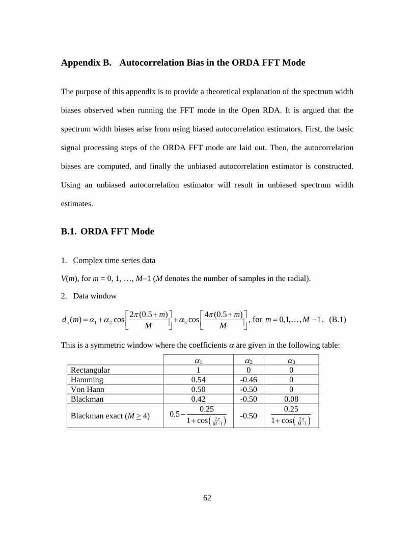
1. Complex time series data

V(m), for m = 0, 1, …, M−1 (M denotes the number of samples in the radial).

2. Data window

1 2 32 (0.5 ) 4 (0.5 )( ) cos cosπ πα α α+ +⎡ ⎤ ⎡ ⎤= + +⎢ ⎥ ⎢ ⎥⎣ ⎦ ⎣ ⎦

um md m

M M, for 0,1, , 1m M= −K . (B.1)

This is a symmetric window where the coefficients α are given in the following table:

α1 α2 α3Rectangular 1 0 0 Hamming 0.54 -0.46 0 Von Hann 0.50 -0.50 0 Blackman 0.42 -0.50 0.08

Blackman exact (M > 4) ( )21

0.250.51 cos M

π−

−+

-0.50 ( )21

0.251 cos M

π−+

62

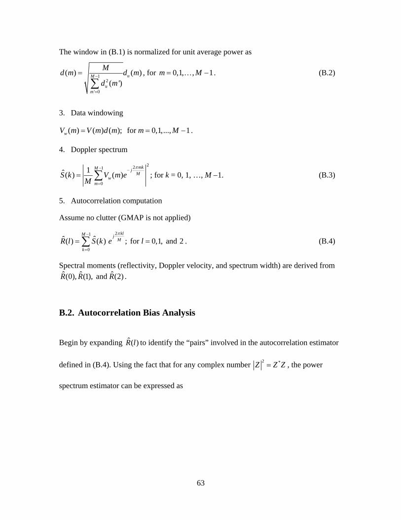
The window in (B.1) is normalized for unit average power as

12

' 0

( ) ( )( ')

−

=

=

∑uM

um

Md m d md m

, for 0,1, , 1m M= −K . (B.2)

3. Data windowing

( ) ( ) ( ); for 0,1,..., 1wV m V m d m m M= = − .

4. Doppler spectrum

221

0

1ˆ( ) ( )π− −

=

= ∑mkM j

Mw

m

S k V m eM

; for k = 0, 1, …, M −1. (B.3)

5. Autocorrelation computation

Assume no clutter (GMAP is not applied)

21

0

ˆˆ( ) ( ) ; for 0,1, and 2klM j

M

kR l S k e l

π−

=

= =∑ . (B.4)

Spectral moments (reflectivity, Doppler velocity, and spectrum width) are derived from ˆ ˆ ˆ(0), (1), and (2)R R R .

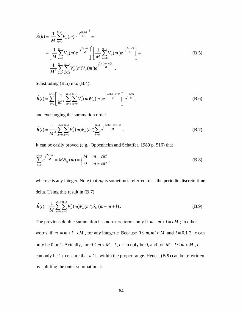
B.2. Autocorrelation Bias Analysis

Begin by expanding ˆ( )R l to identify the “pairs” involved in the autocorrelation estimator

defined in (B.4). Using the fact that for any complex number 2 *Z Z Z= , the power

spectrum estimator can be expressed as

63

2

'− ⎤

⎥⎦

jM

21

0

*2 21 1

0 ' 0

2 ( ')1 1*

20 ' 0

1ˆ( ) ( )

1 1 ( ) ( ')

1 ( ) ( ') .

π

π π

π

− −

=

− −−

= =

−− −

= =

= =

⎡ ⎤ ⎡= =⎢ ⎥ ⎢⎣ ⎦ ⎣

=

∑

∑ ∑

∑∑

mkM jM

wm

mk m kM MjM

w wm m

m m kM M jM

w wm m

S k V m eM

V m e V m eM M

V m V m eM

(B.5)

Substituting (B.5) into (B.4):

2 ( ') 21 1 1 m m k klM M M j*2

0 0 ' 0

1ˆ( ) ( ) ( ') j

M Mw w

k m m

R l V m V m e eM

π π−− − −

⎥= = =

⎡ ⎤= ⎢

⎣ ⎦∑ ∑∑ , (B.6)

and exchanging the summation order

2 ( ' )1 1 1 π − +− − − m m l kM M M*

20 ' 0 0

1ˆ( ) ( ) ( ')= = =

= ∑∑ ∑j

Mw w

m m kR l V m V m e

M. (B.7)

It can be easily proved (e.g., Oppenheim and Schaffer, 1989 p. 516) that

21 π− =mkM

0

( )0

δ=

⎧= = ⎨ ≠⎩

∑j

MM

k

M m cMe M m

m cM, (B.8)

where c is any integer. Note that δM is sometimes referred to as the periodic discrete-time

delta. Using this result in (B.7):

1 1− −

− +M M

*

0 ' 0

1ˆ( ) ( ) ( ') ( ' )δ= =

= ∑∑ w w Mm m

R l V m V m mM

m l

'

. (B.9)

The previous double summation has non-zero terms only if − + =l cM

' = + −m m l cM

m m ; in other

words, if , for any integer c. Because 0 , '≤ <m m M and ; c can

only be 0 or 1. Actually, for , c can only be 0, and for

0,1,2=l

0 ≤ < −m M l − ≤ <M l m M , c

can only be 1 to ensure that m’ is within the proper range. Hence, (B.9) can be re-written

by splitting the outer summation as

64

1 11 − − −

+ +

+

M l M*

0 ' 01 1

*

' 0

ˆ ( ) ( ) ( ') ( ' )

1 ( ) ( ') ( ' ) ,

δ

δ

= =

− −

= − =

= −

+ −

∑ ∑

∑ ∑

w w Mm mM M

w w Mm M l m

R l V m V m m mM

V m V m m m lM

l

'

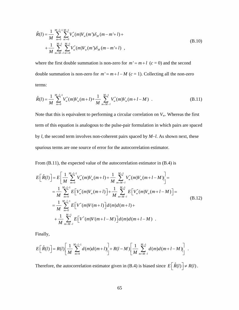
(B.10)

where the first double summation is non-zero for = +m m l

'

(c = 0) and the second

double summation is non-zero for = + −m m l M (c = 1). Collecting all the non-zero

terms:

1 1

( ) (−

= =∑ ∑

M

w wm m M

V m V* *

0

1 1ˆ( ) ( ) ( )+ ) .− −

−

= + + −M l

w wl

R l V m V m l m l MM M

(B.11)

Note that this is equivalent to performing a circular correlation on Vw. Whereas the first

term of this equation is analogous to the pulse-pair formulation in which pairs are spaced

by l, the second term involves non-coherent pairs spaced by M−l. As shown next, these

spurious terms are one source of error for the autocorrelation estimator.

From (B.11), the expected value of the autocorrelation estimator in (B.4) is

1 1− − −

=

⎤− =⎦

M l M* *

0

1 1* *

01

*

0

1 1ˆ( ) ( ) ( ) ( ) ( )

1 1 ( ) ( ) ( ) ( )

1 ( ) ( ) ( ) ( )

= = −

− − −

= = −

− −

=

⎡ ⎤⎡ ⎤ = + + + −⎢ ⎥⎣ ⎦ ⎣ ⎦

⎡ ⎤ ⎡= + + +⎣ ⎦ ⎣

⎡ ⎤= + + +⎣ ⎦

∑ ∑

∑ ∑

∑

w w w wm m M l

M l M

w w w wm m M l

M l

m

E R l E V m V m l V m V m l MM M

E V m V m l E V m V m l MM M

E V m V m l d m d m lM

1*1 ( ) ( ) ( ) ( ) .

−

= −

⎡ ⎤+ + − + −⎣ ⎦∑M

m M l

E V m V m l M d m d m l MM

(B.12)

Finally,

1 1− − − ⎤+ − ⎥⎦

M l M

ˆ

0

1 1ˆ( ) ( ) ( ) ( ) ( ) ( ) ( ) .= = −

⎡ ⎤ ⎡⎡ ⎤ = + + −⎢ ⎥ ⎢⎣ ⎦ ⎣ ⎦ ⎣∑ ∑m m M l

E R l R l d m d m l R l M d m d m l MM M

Therefore, the autocorrelation estimator given in (B.4) is biased since . ( ) ( )E R l R l⎡ ⎤ ≠⎣ ⎦

65

B.3. Unbiased Autocorrelation Estimator

To construct an unbiased autocorrelation estimator, first the spurious terms of (B.11)

must be subtracted; i.e.,

21 1*

0

1ˆˆ( ) ( ) ( ) ( )klM Mj

Mw w

k m M lR l S k e V m V m l

M

π− −

= = −

= − +∑ ∑ M− , (B.13)

which is equivalent [see (B.11)] to

1*

0

1ˆ( ) ( ) ( )M l

w wm

R l V m V mM

− −

=

= ∑ l+ . (B.14)

The expected value of this expression is

1

0

1ˆ( ) ( ) ( ) ( )M l

m

E R l R l d m d m lM

− −

=

⎡⎡ ⎤ = ⎢⎣ ⎦ ⎣ ⎦∑ ⎤+ ⎥ , (B.15)

so it is evident that this modified estimator is still biased by the factor

1

0

1 ( ) ( )− −

=

+∑M l

md m d m l

M . (B.16)

Using (B.13) and (B.15), the unbiased autocorrelation estimator can be constructed as

21 1π− −

−⎦

klM M

ˆ

*

01

0

1ˆ( ) ( ) ( )ˆ( )

1 ( ) ( )

= = −− −

=

⎡ ⎤− +⎢ ⎥⎣=+

∑ ∑

∑

jM

w wk m M l

M l

m

S k e V m V m l MMR l

d m d m lM

. (B.17)

It can be shown now that this estimator is unbiased; i.e., . ( ) ( )⎡ ⎤ =⎣ ⎦E R l R l

66

B.4. Implementation Issues

Note that with the window normalization in (B.2) and for l = 0, 1

0

1 ( ) ( ) 1− −

=

+ =∑M l

md m d m l

M,

so that the unbiased lag-zero autocorrelation estimator reduces to

1

0

ˆˆ(0) ( ) M

kR S k

−

=

= ∑ ; (B.18)

i.e., the lag-zero estimator currently used in the ORDA FFT mode is unbiased regardless

of the data window.

For a rectangular window, 1

0

1 ( ) ( )− −

=

−+ =∑

M l

m

M ld m d m lM M

, a predictable closed-form

solution that results in the unbiased estimator given by

21 1*

0

1ˆˆ( ) ( ) ( ) ( )klM Mj

M

k m M l

MR l S k e V m V m lM l M l

π− −

= = −

⎡= − ⎢− −⎣ ⎦∑ ∑ M ⎤+ − ⎥ . (B.19)

Finally, for aggressive windows 1

*1 ( ) ( ) 0M

w wm M l

V m V m l MM

−

= −

+ − ≈∑ and the estimator can

be simplified to

21

01

0

ˆ( ) ˆ( )

1 ( ) ( )

klM jM

kM l

m

S k eR l

d m d m lM

π−

=− −

=

=+

∑

∑ . (B.20)

67

Note that the same simplification is possible if Vw(m) = 0 for m = M−l, …, M−1; which

can be achieved through zero-padding or simply by forcing the specific data samples to

zero.

68

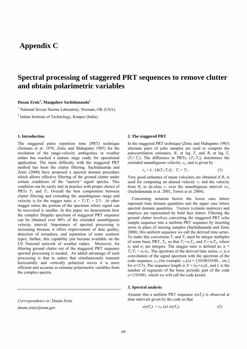
Appendix C

Spectral processing of staggered PRT sequences to remove clutter and obtain polarimetric variables

Dusan Zrnic1, Mangalore Sachidananda2

1 National Severe Storms Laboratory, Norman, OK (USA). 2 Indian Institute of Technology, Kanpur (India).

1. Introduction

The staggered pulse repetition time (PRT) technique (Sirmans et al. 1976, Zrnic and Mahapatra 1985) for the resolution of the range-velocity ambiguities in weather radars has reached a mature stage ready for operational application. The main difficulty with the staggered PRT method has been the clutter filtering. Sachidananda and Zrnic (2000) have proposed a spectral domain procedure which allows effective filtering of the ground clutter under certain conditions of the "narrow" signal spectra. This condition can be easily met in practice with proper choice of PRTs T1 and T2. Overall the best compromise between clutter filtering and extending the unambiguous range and velocity is for the stagger ratio, κ = T1/T2 = 2/3. At other stagger ratios the portion of the spectrum where signal can be recovered is smaller. In this paper we demonstrate how the complex Doppler spectrum of staggered PRT sequence can be obtained over 40% of the extended unambiguous velocity interval. Importance of spectral processing is increasing because it offers improvement of data quality, detection of tornadoes, and separation of some scatterer types; further, this capability just became available on the US National network of weather radars. Moreover, for filtering ground clutter out of the staggered PRT sequence spectral processing is needed. An added advantage of such processing is that in radars that simultaneously transmit horizontally and vertically polarized waves it is more efficient and accurate to estimate polarimetric variables from the complex spectra.

Correspondence to: Dusan Zrnic

dusan.zrnic@noaa.gov

2. The staggered PRT

In the staggered PRT technique (Zrnic and Mahapatra 1985) alternate pairs of echo samples are used to compute the autocorrelation estimates, R1 at lag T1 and R2 at lag T2 (T2>T1). The difference in PRTs, (T2-T1), determines the extended unambiguous velocity, va, and is given by

va = λ / [4(T2-T1)] ; T1 < T2 . (1)

Very good estimates of mean velocities are obtained if R1 is used for computing an aliased velocity v1 and the velocity from R2 to de-alias v1 over the unambiguous interval ±va (Sachidananda et al. 2001, Torres et al. 2004).

Concerning notation herein the lower case letters represent time domain quantities and the upper case letters spectral domain quantities. Vectors (column matrices) and matrices are represented by bold face letters. Filtering the ground clutter involves converting the staggered PRT echo sample sequence into a uniform PRT sequence by inserting zeros in place of missing samples (Sachidananda and Zrnic 2000); this uniform sequence we call the derived time series. To make this conversion T1 and T2 must be integer multiples of some basic PRT, Tu, so that T1=n1Tu, and T2=n2Tu, where n1 and n2 are integers. The stagger ratio is defined as, κ = T1/T2 = n1/n2. The spectrum of the derived time series, e, is a convolution of the signal spectrum with the spectrum of the code sequence, cN (for example, cN(n) = [1010010100... etc.] for κ=2/3). The sequence length is N = (n1+n2)L, and L is the number of segments of the basic periodic part of the code c={10100}, which we will call the code kernel.

3. Spectral analysis

Assume that a uniform PRT sequence s(nTu) is observed at time intervals given by the code so that

e(nTu) = cN (n) s(nTu). (2)

69

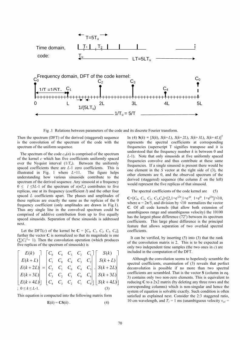
T=5Tu

Tu LT=5LTu

Time domain, code:

1/(5LTu)

1/T =1/5Tu

1/Tu = 5/T

Frequency domain, DFT of the code kernel:

T1 T2

0 L 2L 3L 4L 5L

C0 C1

C2 C3 C4

C0

Fig .1 Relations between parameters of the code and its discrete Fourier transform.

Then the spectrum (DFT) of the derived (staggered) sequence is the convolution of the spectrum of the code with the spectrum of the uniform sequence.

The spectrum of the code cN(n) is comprised of the spectrum of the kernel c which has five coefficients uniformly spaced over the Nyquist interval (1/Tu). Between the uniformly spaced coefficients there are L-1 zero coefficients. This is illustrated in Fig. 1 where L=11. The figure helps understanding how various sinusoids contribute to the spectrum of the derived sequence. Any sinusoid at a frequency 0 ≤ l ≤5L-1 of the spectrum of s(nTu) contributes to five replicas, one at its frequency (coefficient l) and the other four spaced L coefficients apart. The phases and amplitudes of these replicas are exactly the same as the replicas of the 0 frequency coefficient (only amplitudes are drawn in Fig.1). Thus any single line in the convolved spectrum could be comprised of additive contribution from up to five equally spaced sinusoids. Separation of these sinusoids is addressed next.

Let the DFT(c) of the kernel be C = [C0, C1, C2, C3, C4]; further the vector C is normalized so that its magnitude is one (∑|Ci|2= 1). Then the convolution operation (which produces five replicas of the spectrum of sinusoids) is

0 4 3 2 1

1 0 4 3 2

2 1 0 4 3

3 2 1 0 4

4 3 2 1 0

( ) ( )( ) ( )

( 2 ) . ( 2 )( 3 ) ( 3 )( 4 ) ( 4 )

C C C C CE k S kC C C C CE k L S k LC C C C CE k L S k LC C C C CE k L S k LC C C C CE k L S k L

⎡ ⎤⎡ ⎤ ⎡⎢ ⎥⎢ ⎥ ⎢+ ⎢ ⎥⎢ ⎥ ⎢⎢ ⎥+ = +⎢ ⎥ ⎢⎢ ⎥⎢ ⎥ ⎢+ ⎢ ⎥⎢ ⎥ ⎢⎢ ⎥⎢ ⎥ ⎢+⎣ ⎦ ⎣⎣ ⎦

⎤⎥+ ⎥⎥⎥+ ⎥⎥+ ⎦

; 0 ≤ k ≤ L-1. (3)

This equation is compacted into the following matrix form

E(k) = CS(k) . (4)

In (4) S(k) = [S(k), S(k+L), S(k+2L), S(k+3L), S(k+4L)]T represents the spectral coefficients at corresponding frequencies (superscript T signifies transpose and it is understood that the frequency number k is between 0 and L-1). Note that only sinusoids at five uniformly spaced frequencies convolve and thus contribute at these same frequencies. If a single sinusoid is present there would be one element in the S vector at the right side of (3), the other elements are 0, and the observed spectrum of the derived (staggered) sequence (the column E on the left) would represent the five replicas of that sinusoid.

The spectral coefficients of the code kernel are (5)

C=[C0, C1, C2, C3,C4]=[2,1+e-j2α,1+e-jα

, 1+ejα, 1+ej2α]/√10,

where α = 2π/5, and division by √10 normalizes the vector C. Of all code kernels (that allow both extension of unambiguous range and unambiguous velocity) the 10100 has the largest phase difference (72o) between its spectrum coefficients. This large phase difference is the principal feature that allows separation of two overlaid spectral coefficients.

It can be verified, by inserting (5) into (3) that the rank of the convolution matrix is 2. This is to be expected as only two independent time samples (the two ones in c) are included in the computation of the DFT.

Although the convolution seems to hopelessly scramble the spectral coefficients, examination of (3) reveals that perfect deconvolution is possible if no more than two spectral coefficients are scrambled. That is the vector S (column in eq. 3) contains only two non-zero elements. This is equivalent to reducing C to a 2x2 matrix (by deleting any three rows and the corresponding columns) which is non-singular and hence the system of equation is solvable exactly. Such condition is often satisfied as explained next. Consider the 2:3 staggered ratio, 10 cm wavelength, and T1 = 1 ms (unambiguous velocity va1 =

70

25 m s-1, unambiguous range ra1 = 150 km), T2 = 1.5 ms (va2 = 50/3 m s-1, ra2 =225 km); then va = va1va2/( va1-va2) = 100 ms-1. One fifth of va corresponds to the spacing 1/(T1+T2), (i.e., L coefficients out of 5L). If the weather spectrum were to span more than 2L coefficients (40 m s-1) there would be triple overlap of some coefficients and these could not be perfectly retrieved. Otherwise Doppler spectrum occupying ≤ 40 m s-1 interval centered on the mean velocity can be perfectly retrieved. This is certainly a very liberal allowance considering that the largest median values of spectrum width are smaller than 6 m s-1 (Feng et al. 2004)

If the weather spectrum extends exactly over 2L coefficients (i.e., 40% of the interval 5L) then two weather spectral coefficients spaced L units apart will be combined in the convolution process i.e., vector S (has two non-zero elements). Hence the five linear equations represented by (3) are overdetermined. Exact inversion is possible if one knows where the original 2L contiguous spectral coefficients are located within the 5L coefficients. That is, one must know which two of the five elements of S in (3) to retain. An independent location can be obtained using magnitude deconvolution to determine the mean Doppler velocity from such deconvolved spectrum (Sachidananda and Zrnic 2000). That is, the magnitude of the Sd(k), {Sd(k)T = [Sd(k), Sd(k+L), Sd(k+2L), Sd(k+3L), Sd(k+4L)], is computed as

abs[Sd(k)] = abs {[abs(C)]-1abs[E(k)]}, (6)

where the subscript d signifies that the spectrum coefficient comes from deconvolution. After the operation (6) is completed L times (once for each k) there would be L sets of five replicas, each set separated by one coefficient from its adjacent neighbor (spectrum line). Thus the recombined sequence of spectrum coefficients is Sd(0), Sd(1), Sd(2)... Sd(L), Sd(L+1), Sd(L+2),... Sd(2L), Sd(2L+1), Sd(2L+2)........ Sd(4L), Sd(4L+1),... Sd(5L-1).

If there are at least two spectral components (sinusoids) spaced a multiple of L coefficients apart, for example S(k) and S(k+L), the Sd(k) will differ from S(k) of the uniform PRT sequence and so would Sd(k+L) from S(k+L).

The mean velocity (frequency) of the deconvolved spectrum locates the center of the original spectrum. Suppose that this mean corresponds to the coefficient m and m<L, then the S(k)T = [S(k), S(k+L), 0, 0, 0] should be used in (3) for m ≤ k ≤ m+L/2, (if L is odd subtract one from L and adjust so that all L coefficients are considered). For coefficients between m-L/2 and m the reconstruction should take S(k)T = [S(k), 0, 0, 0, S(k+4L)].

4. Practical aspects

The reconstruction thus far considers a spectrum in which two coefficients are contiguous, i.e., separated by L lines. In some situations significant coefficients can be separated by 2L or 3L segments (larger circular separation is not possible). Such separation is often between coefficient of weather signal and ground clutter (or fast moving objects).

In cases that the ground clutter in the derived sequence overlaps weather spectra, clutter replicas must be removed (set to zero) to correctly locate the position of the weather spectrum via (6). Then the clutter complex spectral component and one weather component can be obtained. Thus the two strongest components can be retrieved provided that other components are negligible.

Al low SNRs reconstruction of spectra is difficult and more so is the separation of overlapping spectral components. Five noise components overlay each other and if these have powers comparable to the signal power the retrieval fails. Spectral components of comparable power but separated by more than 2L coefficients (e.g., one due to aircraft traffic the other due to weather) are also hard to separate because there might not be a simple way to determine the correct (original) location of these components.

Complex spectra are needed for computing the polarimetric variables after removal of ground clutter from the staggered PRT sequence. Further such spectra can be useful for detecting small tornadoes within the radar resolution volume.

Results (to be presented at this conference) indicate that the clutter filtering coupled with the spectrum recovery algorithm is very effective in processing staggered PRT sequence from dual-polarized radar. The fields of the polarimetric variables thus obtained at 0.44o elevation exhibit spatial continuity and an order of magnitude reduction of clutter contaminated area.

5. References

Fang, M., R.J. Doviak, and V. Melnikov, 2004: Spectrum width measured by WSR-88D: error sources and statistics of various weather phenomena. J. Atmos. Oceanic Technol., 21, 888-904.

Sachidananda, M., and D. S. Zrnic, 2000: Clutter filtering and spectral moment estimation for Doppler weather radars using staggered pulse repetition time (PRT). J. Atmos. Oceanic Technol., 17, 323-331.

Sachidananda, M., D. S. Zrnic, and R. J. Doviak, 2001: Signal design and processing techniques for WSR-88D ambiguity resolution. Report, Part-5. National Severe Storms Laboratory, October 2001, 70 pp.

Sirmans, D., D. Zrnic, and B. Bumgarner, 1976: Extension of maximum unambiguous Doppler velocity by use of two sampling rates. Preprints, 17th Conference on Radar Meteorology. Seattle, WA, Amer. Meteor. Soc., 23-28.

Torres, M. S., Y. F. Dubel, and D. S. Zrnic, 2004: Design, implementation, and demonstration of a staggered PRT algorithm for the WSR-88D. J. Atmos. Oceanic Technol., 21, 1389-1399.

Zrnic, D. S., and P. R. Mahapatra, 1985: Two methods of ambiguity resolution in pulsed Doppler weather radars. IEEE Trans. on Aerospace and Electronic Systems, AES-21, 470-483.

71