signal processing toolbox - cvut.czradio.feld.cvut.cz/matlab/pdf_doc/signal/signal_tb.pdf ·...
TRANSCRIPT
Computation
Visualization
Programming
For Use with MATLAB®
User’s GuideVersion 5
Signal ProcessingToolbox
How to Contact The MathWorks:
508-647-7000 Phone
508-647-7001 Fax
The MathWorks, Inc. Mail3 Apple Hill DriveNatick, MA 01760-2098
http://www.mathworks.com Webftp.mathworks.com Anonymous FTP servercomp.soft-sys.matlab Newsgroup
[email protected] Technical [email protected] Product enhancement [email protected] Bug [email protected] Documentation error [email protected] Subscribing user [email protected] Order status, license renewals, [email protected] Sales, pricing, and general information
Signal Processing Toolbox User’s Guide COPYRIGHT 1988 - 2000 by The MathWorks, Inc.The software described in this document is furnished under a license agreement. The software may be usedor copied only under the terms of the license agreement. No part of this manual may be photocopied or repro-duced in any form without prior written consent from The MathWorks, Inc.
FEDERAL ACQUISITION: This provision applies to all acquisitions of the Program and Documentation byor for the federal government of the United States. By accepting delivery of the Program, the governmenthereby agrees that this software qualifies as "commercial" computer software within the meaning of FARPart 12.212, DFARS Part 227.7202-1, DFARS Part 227.7202-3, DFARS Part 252.227-7013, and DFARS Part252.227-7014. The terms and conditions of The MathWorks, Inc. Software License Agreement shall pertainto the government’s use and disclosure of the Program and Documentation, and shall supersede anyconflicting contractual terms or conditions. If this license fails to meet the government’s minimum needs oris inconsistent in any respect with federal procurement law, the government agrees to return the Programand Documentation, unused, to MathWorks.
MATLAB, Simulink, Stateflow, Handle Graphics, and Real-Time Workshop are registered trademarks, andTarget Language Compiler is a trademark of The MathWorks, Inc.
Other product or brand names are trademarks or registered trademarks of their respective holders.
Printing History: January 1997 First printing New for MATLAB 5.1January 1998 Second printingRevised for MATLAB 5.2January 1999 (Online Only) Revised for Version 4.2 (Release 11)August 1999 (Online Only) Revised for Version 4.3 (Release 11)September 2000 Third printing Revised for Version 5.0 (Release 12)
i
Contents
Preface
Overview . . . . . . . . . . . . . . . . . . . . . . . . . . . . . . . . . . . . . . . . . . . . . 22
What Is the Signal Processing Toolbox? . . . . . . . . . . . . . . . . . . 23
R12 Related Products List . . . . . . . . . . . . . . . . . . . . . . . . . . . . . . 24
How to Use This Manual . . . . . . . . . . . . . . . . . . . . . . . . . . . . . . . . 26If You Are a New User . . . . . . . . . . . . . . . . . . . . . . . . . . . . . . . . . 26If You Are an Experienced Toolbox User . . . . . . . . . . . . . . . . . . . 27All Toolbox Users . . . . . . . . . . . . . . . . . . . . . . . . . . . . . . . . . . . . . . 27
Installing the Signal Processing Toolbox . . . . . . . . . . . . . . . . . 28
Technical Conventions . . . . . . . . . . . . . . . . . . . . . . . . . . . . . . . . . 29
Typographical Conventions . . . . . . . . . . . . . . . . . . . . . . . . . . . . 30
1Signal Processing Basics
Overview . . . . . . . . . . . . . . . . . . . . . . . . . . . . . . . . . . . . . . . . . . . . 1-2
Signal Processing Toolbox Central Features . . . . . . . . . . . . 1-3Filtering and FFTs . . . . . . . . . . . . . . . . . . . . . . . . . . . . . . . . . . . 1-3Signals and Systems . . . . . . . . . . . . . . . . . . . . . . . . . . . . . . . . . . 1-3Key Areas: Filter Design and Spectral Analysis . . . . . . . . . . . . 1-3Interactive Tools: SPTool and FDATool . . . . . . . . . . . . . . . . . . . 1-4Extensibility . . . . . . . . . . . . . . . . . . . . . . . . . . . . . . . . . . . . . . . . . 1-4
ii Contents
Representing Signals . . . . . . . . . . . . . . . . . . . . . . . . . . . . . . . . . . 1-5Vector Representation . . . . . . . . . . . . . . . . . . . . . . . . . . . . . . . . . 1-5
Waveform Generation: Time Vectors and Sinusoids . . . . . . 1-7Common Sequences: Unit Impulse, Unit Step, and Unit Ramp 1-8Multichannel Signals . . . . . . . . . . . . . . . . . . . . . . . . . . . . . . . . . . 1-8Common Periodic Waveforms . . . . . . . . . . . . . . . . . . . . . . . . . . . 1-9Common Aperiodic Waveforms . . . . . . . . . . . . . . . . . . . . . . . . . 1-10The pulstran Function . . . . . . . . . . . . . . . . . . . . . . . . . . . . . . . . 1-11The Sinc Function . . . . . . . . . . . . . . . . . . . . . . . . . . . . . . . . . . . 1-12The Dirichlet Function . . . . . . . . . . . . . . . . . . . . . . . . . . . . . . . 1-13
Working with Data . . . . . . . . . . . . . . . . . . . . . . . . . . . . . . . . . . . 1-14
Filter Implementation and Analysis . . . . . . . . . . . . . . . . . . . 1-15Convolution and Filtering . . . . . . . . . . . . . . . . . . . . . . . . . . . . . 1-15Filters and Transfer Functions . . . . . . . . . . . . . . . . . . . . . . . . . 1-16
Filter Coefficients and Filter Names . . . . . . . . . . . . . . . . . . 1-16Filtering with the filter Function . . . . . . . . . . . . . . . . . . . . . . . 1-17
The filter Function . . . . . . . . . . . . . . . . . . . . . . . . . . . . . . . . . . . 1-18
Other Functions for Filtering . . . . . . . . . . . . . . . . . . . . . . . . . 1-20Multirate Filter Bank Implementation . . . . . . . . . . . . . . . . . . 1-20Anti-Causal, Zero-Phase Filter Implementation . . . . . . . . . . . 1-21Frequency Domain Filter Implementation . . . . . . . . . . . . . . . . 1-23
Impulse Response . . . . . . . . . . . . . . . . . . . . . . . . . . . . . . . . . . . . 1-24
Frequency Response . . . . . . . . . . . . . . . . . . . . . . . . . . . . . . . . . 1-25Digital Domain . . . . . . . . . . . . . . . . . . . . . . . . . . . . . . . . . . . . . . 1-25Analog Domain . . . . . . . . . . . . . . . . . . . . . . . . . . . . . . . . . . . . . . 1-27Magnitude and Phase . . . . . . . . . . . . . . . . . . . . . . . . . . . . . . . . 1-27Delay . . . . . . . . . . . . . . . . . . . . . . . . . . . . . . . . . . . . . . . . . . . . . . 1-29
Zero-Pole Analysis . . . . . . . . . . . . . . . . . . . . . . . . . . . . . . . . . . . 1-31
Linear System Models . . . . . . . . . . . . . . . . . . . . . . . . . . . . . . . . 1-33Discrete-Time System Models . . . . . . . . . . . . . . . . . . . . . . . . . . 1-33
iii
Transfer Function . . . . . . . . . . . . . . . . . . . . . . . . . . . . . . . . . 1-33Zero-Pole-Gain . . . . . . . . . . . . . . . . . . . . . . . . . . . . . . . . . . . . 1-34State-Space . . . . . . . . . . . . . . . . . . . . . . . . . . . . . . . . . . . . . . 1-35Partial Fraction Expansion (Residue Form) . . . . . . . . . . . . 1-36Second-Order Sections (SOS) . . . . . . . . . . . . . . . . . . . . . . . . 1-38Lattice Structure . . . . . . . . . . . . . . . . . . . . . . . . . . . . . . . . . . 1-38Convolution Matrix . . . . . . . . . . . . . . . . . . . . . . . . . . . . . . . . 1-41
Continuous-Time System Models . . . . . . . . . . . . . . . . . . . . . . . 1-42Linear System Transformations . . . . . . . . . . . . . . . . . . . . . . . . 1-43
Discrete Fourier Transform . . . . . . . . . . . . . . . . . . . . . . . . . . . 1-45
Selected Bibliography . . . . . . . . . . . . . . . . . . . . . . . . . . . . . . . . 1-48
2Filter Design
Overview . . . . . . . . . . . . . . . . . . . . . . . . . . . . . . . . . . . . . . . . . . . . . 2-2
Filter Requirements and Specification . . . . . . . . . . . . . . . . . . 2-3
IIR Filter Design . . . . . . . . . . . . . . . . . . . . . . . . . . . . . . . . . . . . . . 2-5Classical IIR Filter Design Using Analog Prototyping . . . . . . . 2-7
Complete Classical IIR Filter Design . . . . . . . . . . . . . . . . . . . 2-7Designing IIR Filters to Frequency Domain Specifications . 2-8
Comparison of Classical IIR Filter Types . . . . . . . . . . . . . . . . . . 2-9Butterworth Filter . . . . . . . . . . . . . . . . . . . . . . . . . . . . . . . . . . 2-9Chebyshev Type I Filter . . . . . . . . . . . . . . . . . . . . . . . . . . . . 2-10Chebyshev Type II Filter . . . . . . . . . . . . . . . . . . . . . . . . . . . . 2-11Elliptic Filter . . . . . . . . . . . . . . . . . . . . . . . . . . . . . . . . . . . . . 2-11Bessel Filter . . . . . . . . . . . . . . . . . . . . . . . . . . . . . . . . . . . . . . 2-12Direct IIR Filter Design . . . . . . . . . . . . . . . . . . . . . . . . . . . . 2-14Generalized Butterworth Filter Design . . . . . . . . . . . . . . . . 2-15
FIR Filter Design . . . . . . . . . . . . . . . . . . . . . . . . . . . . . . . . . . . . 2-17Linear Phase Filters . . . . . . . . . . . . . . . . . . . . . . . . . . . . . . . . . 2-18Windowing Method . . . . . . . . . . . . . . . . . . . . . . . . . . . . . . . . . . 2-19
iv Contents
Standard Band FIR Filter Design: fir1 . . . . . . . . . . . . . . . . 2-21Multiband FIR Filter Design: fir2 . . . . . . . . . . . . . . . . . . . . 2-22
Multiband FIR Filter Design with Transition Bands . . . . . . . 2-23Basic Configurations . . . . . . . . . . . . . . . . . . . . . . . . . . . . . . . 2-23The Weight Vector . . . . . . . . . . . . . . . . . . . . . . . . . . . . . . . . . 2-26Anti-Symmetric Filters / Hilbert Transformers . . . . . . . . . . 2-26Differentiators . . . . . . . . . . . . . . . . . . . . . . . . . . . . . . . . . . . . 2-27
Constrained Least Squares FIR Filter Design . . . . . . . . . . . . . 2-28Basic Lowpass and Highpass CLS Filter Design . . . . . . . . . 2-29Multiband CLS Filter Design . . . . . . . . . . . . . . . . . . . . . . . . 2-30Weighted CLS Filter Design . . . . . . . . . . . . . . . . . . . . . . . . . 2-31
Arbitrary-Response Filter Design . . . . . . . . . . . . . . . . . . . . . . . 2-32Multiband Filter Design . . . . . . . . . . . . . . . . . . . . . . . . . . . . 2-33Filter Design with Reduced Delay . . . . . . . . . . . . . . . . . . . . 2-35
Special Topics in IIR Filter Design . . . . . . . . . . . . . . . . . . . . 2-38Analog Prototype Design . . . . . . . . . . . . . . . . . . . . . . . . . . . . . . 2-39Frequency Transformation . . . . . . . . . . . . . . . . . . . . . . . . . . . . 2-39Filter Discretization . . . . . . . . . . . . . . . . . . . . . . . . . . . . . . . . . . 2-42
Impulse Invariance . . . . . . . . . . . . . . . . . . . . . . . . . . . . . . . . 2-42Bilinear Transformation . . . . . . . . . . . . . . . . . . . . . . . . . . . . 2-43
Selected Bibliography . . . . . . . . . . . . . . . . . . . . . . . . . . . . . . . . 2-46
3Statistical Signal Processing
Overview . . . . . . . . . . . . . . . . . . . . . . . . . . . . . . . . . . . . . . . . . . . . . 3-2
Correlation and Covariance . . . . . . . . . . . . . . . . . . . . . . . . . . . . 3-3Bias and Normalization . . . . . . . . . . . . . . . . . . . . . . . . . . . . . . . . 3-4Multiple Channels . . . . . . . . . . . . . . . . . . . . . . . . . . . . . . . . . . . . 3-5
Spectral Analysis . . . . . . . . . . . . . . . . . . . . . . . . . . . . . . . . . . . . . 3-6Spectral Estimation Method Overview . . . . . . . . . . . . . . . . . . . . 3-8Nonparametric Methods . . . . . . . . . . . . . . . . . . . . . . . . . . . . . . 3-10
The Periodogram . . . . . . . . . . . . . . . . . . . . . . . . . . . . . . . . . . 3-10
v
Performance of the Periodogram 3-12The Modified Periodogram . . . . . . . . . . . . . . . . . . . . . . . . . . 3-18Welch’s Method . . . . . . . . . . . . . . . . . . . . . . . . . . . . . . . . . . . 3-20Bias and Normalization in Welch’s Method . . . . . . . . . . . . . 3-23Multitaper Method . . . . . . . . . . . . . . . . . . . . . . . . . . . . . . . . . 3-24Cross-Spectral Density Function . . . . . . . . . . . . . . . . . . . . . 3-27Confidence Intervals . . . . . . . . . . . . . . . . . . . . . . . . . . . . . . . 3-27Transfer Function Estimate . . . . . . . . . . . . . . . . . . . . . . . . . 3-28Coherence Function . . . . . . . . . . . . . . . . . . . . . . . . . . . . . . . . 3-29
Parametric Methods . . . . . . . . . . . . . . . . . . . . . . . . . . . . . . . . . . 3-30Yule-Walker AR Method . . . . . . . . . . . . . . . . . . . . . . . . . . . . 3-32Burg Method . . . . . . . . . . . . . . . . . . . . . . . . . . . . . . . . . . . . . 3-33Covariance and Modified Covariance Methods . . . . . . . . . . 3-36MUSIC and Eigenvector Analysis Methods . . . . . . . . . . . . . 3-36Eigenanalysis Overview . . . . . . . . . . . . . . . . . . . . . . . . . . . . 3-37
Selected Bibliography . . . . . . . . . . . . . . . . . . . . . . . . . . . . . . . . 3-39
4Special Topics
Overview . . . . . . . . . . . . . . . . . . . . . . . . . . . . . . . . . . . . . . . . . . . . . 4-2
Windows . . . . . . . . . . . . . . . . . . . . . . . . . . . . . . . . . . . . . . . . . . . . . 4-3Basic Shapes . . . . . . . . . . . . . . . . . . . . . . . . . . . . . . . . . . . . . . . . . 4-3Generalized Cosine Windows . . . . . . . . . . . . . . . . . . . . . . . . . . . 4-5Kaiser Window . . . . . . . . . . . . . . . . . . . . . . . . . . . . . . . . . . . . . . . 4-5
Kaiser Windows in FIR Design . . . . . . . . . . . . . . . . . . . . . . . . 4-7Chebyshev Window . . . . . . . . . . . . . . . . . . . . . . . . . . . . . . . . . . . 4-9
Parametric Modeling . . . . . . . . . . . . . . . . . . . . . . . . . . . . . . . . . 4-11Time-Domain Based Modeling . . . . . . . . . . . . . . . . . . . . . . . . . 4-13
Linear Prediction . . . . . . . . . . . . . . . . . . . . . . . . . . . . . . . . . . 4-13Prony’s Method (ARMA Modeling) . . . . . . . . . . . . . . . . . . . . 4-14Steiglitz-McBride Method (ARMA Modeling) . . . . . . . . . . . 4-16
Frequency-Domain Based Modeling . . . . . . . . . . . . . . . . . . . . . 4-18
vi Contents
Resampling . . . . . . . . . . . . . . . . . . . . . . . . . . . . . . . . . . . . . . . . . . 4-21
Cepstrum Analysis . . . . . . . . . . . . . . . . . . . . . . . . . . . . . . . . . . . 4-24Inverse Complex Cepstrum . . . . . . . . . . . . . . . . . . . . . . . . . . . . 4-26
FFT-Based Time-Frequency Analysis . . . . . . . . . . . . . . . . . . 4-28
Median Filtering . . . . . . . . . . . . . . . . . . . . . . . . . . . . . . . . . . . . . 4-29
Communications Applications . . . . . . . . . . . . . . . . . . . . . . . . . 4-30
Deconvolution . . . . . . . . . . . . . . . . . . . . . . . . . . . . . . . . . . . . . . . 4-34
Specialized Transforms . . . . . . . . . . . . . . . . . . . . . . . . . . . . . . . 4-35Chirp z-Transform . . . . . . . . . . . . . . . . . . . . . . . . . . . . . . . . . . . 4-35Discrete Cosine Transform . . . . . . . . . . . . . . . . . . . . . . . . . . . . 4-37Hilbert Transform . . . . . . . . . . . . . . . . . . . . . . . . . . . . . . . . . . . 4-39
Selected Bibliography . . . . . . . . . . . . . . . . . . . . . . . . . . . . . . . . 4-41
5Filter Design and Analysis Tool
Overview . . . . . . . . . . . . . . . . . . . . . . . . . . . . . . . . . . . . . . . . . . . . . 5-2Filter Design Methods . . . . . . . . . . . . . . . . . . . . . . . . . . . . . . . . . 5-2Using the Filter Design and Analysis Tool . . . . . . . . . . . . . . . . . 5-3Analyzing Filter Responses . . . . . . . . . . . . . . . . . . . . . . . . . . . . . 5-3Filter Design and Analysis Tool Modes . . . . . . . . . . . . . . . . . . . 5-3Getting Help . . . . . . . . . . . . . . . . . . . . . . . . . . . . . . . . . . . . . . . . . 5-4
Opening the Filter Design and Analysis Tool . . . . . . . . . . . . 5-5
Getting Help . . . . . . . . . . . . . . . . . . . . . . . . . . . . . . . . . . . . . . . . . . 5-6Context-Sensitive Help: The What’s This? Button . . . . . . . . . . 5-6
Choosing a Filter Type . . . . . . . . . . . . . . . . . . . . . . . . . . . . . . . . 5-7
vii
Choosing a Filter Design Method . . . . . . . . . . . . . . . . . . . . . . . 5-8
Setting the Filter Design Specifications . . . . . . . . . . . . . . . . . 5-9Bandpass Filter Frequency Specifications . . . . . . . . . . . . . . . . . 5-9Bandpass Filter Magnitude Specifications . . . . . . . . . . . . . . . . 5-10Filter Order . . . . . . . . . . . . . . . . . . . . . . . . . . . . . . . . . . . . . . . . 5-11
Computing the Filter Coefficients . . . . . . . . . . . . . . . . . . . . . 5-12
Analyzing the Filter . . . . . . . . . . . . . . . . . . . . . . . . . . . . . . . . . . 5-13
Converting the Filter Structure . . . . . . . . . . . . . . . . . . . . . . . 5-14
Importing a Filter Design . . . . . . . . . . . . . . . . . . . . . . . . . . . . . 5-16Filter Structures . . . . . . . . . . . . . . . . . . . . . . . . . . . . . . . . . . . . 5-17
Direct Form . . . . . . . . . . . . . . . . . . . . . . . . . . . . . . . . . . . . . . 5-17Direct Form II (Second-Order Sections) . . . . . . . . . . . . . . . . 5-17State-Space . . . . . . . . . . . . . . . . . . . . . . . . . . . . . . . . . . . . . . 5-18Lattice . . . . . . . . . . . . . . . . . . . . . . . . . . . . . . . . . . . . . . . . . . . 5-18Quantized Filter (Qfilt Object) . . . . . . . . . . . . . . . . . . . . . . . 5-18
Exporting a Filter Design . . . . . . . . . . . . . . . . . . . . . . . . . . . . . 5-19Exporting Filter Coefficients to the Workspace . . . . . . . . . . . . 5-19Exporting Filter Coefficients to a Text File . . . . . . . . . . . . . . . 5-20
Saving and Opening Filter Design Sessions . . . . . . . . . . . . . 5-21
6SPTool: A Signal Processing GUI Suite
Overview . . . . . . . . . . . . . . . . . . . . . . . . . . . . . . . . . . . . . . . . . . . . . 6-2
SPTool: An Interactive Signal Processing Environment . . 6-3SPTool Data Structures . . . . . . . . . . . . . . . . . . . . . . . . . . . . . . . . 6-4
Opening SPTool . . . . . . . . . . . . . . . . . . . . . . . . . . . . . . . . . . . . . . . 6-5
viii Contents
Overview of the Signal Browser: Signal Analysis . . . . . . . . . 6-6Opening the Signal Browser . . . . . . . . . . . . . . . . . . . . . . . . . . . . 6-6
Overview of the Filter Designer: Filter Design . . . . . . . . . . . 6-8Filter Types . . . . . . . . . . . . . . . . . . . . . . . . . . . . . . . . . . . . . . . . . 6-8FIR Filter Methods . . . . . . . . . . . . . . . . . . . . . . . . . . . . . . . . . . . 6-8IIR Filter Methods . . . . . . . . . . . . . . . . . . . . . . . . . . . . . . . . . . . . 6-8Pole/Zero Editor . . . . . . . . . . . . . . . . . . . . . . . . . . . . . . . . . . . . . . 6-9Spectral Overlay Feature . . . . . . . . . . . . . . . . . . . . . . . . . . . . . . 6-9Opening the Filter Designer . . . . . . . . . . . . . . . . . . . . . . . . . . . . 6-9
Overview of the Filter Viewer: Filter Analysis . . . . . . . . . . 6-11Opening the Filter Viewer . . . . . . . . . . . . . . . . . . . . . . . . . . . . . 6-11
Overview of the Spectrum Viewer: Spectral Analysis . . . . 6-14Opening the Spectrum Viewer . . . . . . . . . . . . . . . . . . . . . . . . . 6-14
Getting Help . . . . . . . . . . . . . . . . . . . . . . . . . . . . . . . . . . . . . . . . . 6-17Context-Sensitive Help: The What’s This? Button . . . . . . . . . 6-17
Using SPTool: Filtering and Analysis of Noise . . . . . . . . . . 6-18
Importing a Signal into SPTool . . . . . . . . . . . . . . . . . . . . . . . . 6-19
Designing a Filter . . . . . . . . . . . . . . . . . . . . . . . . . . . . . . . . . . . . 6-22Opening the Filter Designer . . . . . . . . . . . . . . . . . . . . . . . . . . . 6-22Specifying the Bandpass Filter . . . . . . . . . . . . . . . . . . . . . . . . . 6-22
Applying a Filter to a Signal . . . . . . . . . . . . . . . . . . . . . . . . . . 6-24
Analyzing Signals: Opening the Signal Browser . . . . . . . . . 6-26Playing a Signal . . . . . . . . . . . . . . . . . . . . . . . . . . . . . . . . . . . . . 6-27Printing a Signal . . . . . . . . . . . . . . . . . . . . . . . . . . . . . . . . . . . . 6-28
Spectral Analysis in the Spectrum Viewer . . . . . . . . . . . . . . 6-29Creating a PSD Object From a Signal . . . . . . . . . . . . . . . . . . . 6-29Opening the Spectrum Viewer with Two Spectra . . . . . . . . . . 6-30Printing the Spectra . . . . . . . . . . . . . . . . . . . . . . . . . . . . . . . . . 6-31
ix
Exporting Signals, Filters, and Spectra . . . . . . . . . . . . . . . . 6-32Opening the Export Dialog Box . . . . . . . . . . . . . . . . . . . . . . . . . 6-32
Exporting a Filter to the MATLAB Workspace . . . . . . . . . . 6-33
Designing a Filter with the Pole/Zero Editor . . . . . . . . . . . . 6-34Positioning Poles and Zeros . . . . . . . . . . . . . . . . . . . . . . . . . . . . 6-35
Redesigning a Filter Using the Magnitude Plot . . . . . . . . . 6-37
Accessing Filter Parameters in a Saved Filter . . . . . . . . . . 6-38The tf Field: Accessing Filter Coefficients . . . . . . . . . . . . . . . . 6-38The Fs Field: Accessing Filter Sample Frequency . . . . . . . . . . 6-38The specs Field: Accessing other Filter Parameters . . . . . . . . 6-39
Accessing Parameters in a Saved Spectrum . . . . . . . . . . . . 6-42
Importing Filters and Spectra into SPTool . . . . . . . . . . . . . 6-43Importing Filters . . . . . . . . . . . . . . . . . . . . . . . . . . . . . . . . . . . . 6-43Importing Spectra . . . . . . . . . . . . . . . . . . . . . . . . . . . . . . . . . . . 6-45
Loading Variables from the Disk . . . . . . . . . . . . . . . . . . . . . . 6-47
Selecting Signals, Filters, and Spectra in SPTool . . . . . . . . 6-48
Editing Signals, Filters, or Spectra in SPTool . . . . . . . . . . . 6-49
Setting Preferences . . . . . . . . . . . . . . . . . . . . . . . . . . . . . . . . . . 6-50
Making Signal Measurements: Using Markers . . . . . . . . . . 6-51
7Function Reference
Function Category List . . . . . . . . . . . . . . . . . . . . . . . . . . . . . . . . 7-3abs . . . . . . . . . . . . . . . . . . . . . . . . . . . . . . . . . . . . . . . . . . . . . . . . 7-16ac2poly . . . . . . . . . . . . . . . . . . . . . . . . . . . . . . . . . . . . . . . . . . . . 7-17

x Contents
ac2rc . . . . . . . . . . . . . . . . . . . . . . . . . . . . . . . . . . . . . . . . . . . . . . 7-18angle . . . . . . . . . . . . . . . . . . . . . . . . . . . . . . . . . . . . . . . . . . . . . . 7-19arburg . . . . . . . . . . . . . . . . . . . . . . . . . . . . . . . . . . . . . . . . . . . . . 7-20arcov . . . . . . . . . . . . . . . . . . . . . . . . . . . . . . . . . . . . . . . . . . . . . . 7-21armcov . . . . . . . . . . . . . . . . . . . . . . . . . . . . . . . . . . . . . . . . . . . . 7-22aryule . . . . . . . . . . . . . . . . . . . . . . . . . . . . . . . . . . . . . . . . . . . . . 7-23bartlett . . . . . . . . . . . . . . . . . . . . . . . . . . . . . . . . . . . . . . . . . . . . 7-24besselap . . . . . . . . . . . . . . . . . . . . . . . . . . . . . . . . . . . . . . . . . . . 7-26besself . . . . . . . . . . . . . . . . . . . . . . . . . . . . . . . . . . . . . . . . . . . . . 7-27bilinear . . . . . . . . . . . . . . . . . . . . . . . . . . . . . . . . . . . . . . . . . . . . 7-31blackman . . . . . . . . . . . . . . . . . . . . . . . . . . . . . . . . . . . . . . . . . . 7-36boxcar . . . . . . . . . . . . . . . . . . . . . . . . . . . . . . . . . . . . . . . . . . . . . 7-38buffer . . . . . . . . . . . . . . . . . . . . . . . . . . . . . . . . . . . . . . . . . . . . . . 7-39buttap . . . . . . . . . . . . . . . . . . . . . . . . . . . . . . . . . . . . . . . . . . . . . 7-48butter . . . . . . . . . . . . . . . . . . . . . . . . . . . . . . . . . . . . . . . . . . . . . 7-49buttord . . . . . . . . . . . . . . . . . . . . . . . . . . . . . . . . . . . . . . . . . . . . 7-54cceps . . . . . . . . . . . . . . . . . . . . . . . . . . . . . . . . . . . . . . . . . . . . . . 7-59cell2sos . . . . . . . . . . . . . . . . . . . . . . . . . . . . . . . . . . . . . . . . . . . . 7-61cheb1ap . . . . . . . . . . . . . . . . . . . . . . . . . . . . . . . . . . . . . . . . . . . . 7-62cheb1ord . . . . . . . . . . . . . . . . . . . . . . . . . . . . . . . . . . . . . . . . . . . 7-63cheb2ap . . . . . . . . . . . . . . . . . . . . . . . . . . . . . . . . . . . . . . . . . . . . 7-67cheb2ord . . . . . . . . . . . . . . . . . . . . . . . . . . . . . . . . . . . . . . . . . . . 7-68chebwin . . . . . . . . . . . . . . . . . . . . . . . . . . . . . . . . . . . . . . . . . . . . 7-73cheby1 . . . . . . . . . . . . . . . . . . . . . . . . . . . . . . . . . . . . . . . . . . . . . 7-75cheby2 . . . . . . . . . . . . . . . . . . . . . . . . . . . . . . . . . . . . . . . . . . . . . 7-80chirp . . . . . . . . . . . . . . . . . . . . . . . . . . . . . . . . . . . . . . . . . . . . . . 7-85cohere . . . . . . . . . . . . . . . . . . . . . . . . . . . . . . . . . . . . . . . . . . . . . 7-88conv . . . . . . . . . . . . . . . . . . . . . . . . . . . . . . . . . . . . . . . . . . . . . . . 7-92conv2 . . . . . . . . . . . . . . . . . . . . . . . . . . . . . . . . . . . . . . . . . . . . . . 7-93convmtx . . . . . . . . . . . . . . . . . . . . . . . . . . . . . . . . . . . . . . . . . . . . 7-95corrcoef . . . . . . . . . . . . . . . . . . . . . . . . . . . . . . . . . . . . . . . . . . . . 7-97corrmtx . . . . . . . . . . . . . . . . . . . . . . . . . . . . . . . . . . . . . . . . . . . . 7-98cov . . . . . . . . . . . . . . . . . . . . . . . . . . . . . . . . . . . . . . . . . . . . . . . 7-101cplxpair . . . . . . . . . . . . . . . . . . . . . . . . . . . . . . . . . . . . . . . . . . . 7-102cremez . . . . . . . . . . . . . . . . . . . . . . . . . . . . . . . . . . . . . . . . . . . . 7-103csd . . . . . . . . . . . . . . . . . . . . . . . . . . . . . . . . . . . . . . . . . . . . . . . 7-111czt . . . . . . . . . . . . . . . . . . . . . . . . . . . . . . . . . . . . . . . . . . . . . . . 7-116dct . . . . . . . . . . . . . . . . . . . . . . . . . . . . . . . . . . . . . . . . . . . . . . . 7-119decimate . . . . . . . . . . . . . . . . . . . . . . . . . . . . . . . . . . . . . . . . . . 7-121deconv . . . . . . . . . . . . . . . . . . . . . . . . . . . . . . . . . . . . . . . . . . . . 7-124
xi
demod . . . . . . . . . . . . . . . . . . . . . . . . . . . . . . . . . . . . . . . . . . . . 7-125dftmtx . . . . . . . . . . . . . . . . . . . . . . . . . . . . . . . . . . . . . . . . . . . . 7-127diric . . . . . . . . . . . . . . . . . . . . . . . . . . . . . . . . . . . . . . . . . . . . . . 7-128dpss . . . . . . . . . . . . . . . . . . . . . . . . . . . . . . . . . . . . . . . . . . . . . . 7-129dpssclear . . . . . . . . . . . . . . . . . . . . . . . . . . . . . . . . . . . . . . . . . . 7-132dpssdir . . . . . . . . . . . . . . . . . . . . . . . . . . . . . . . . . . . . . . . . . . . 7-133dpssload . . . . . . . . . . . . . . . . . . . . . . . . . . . . . . . . . . . . . . . . . . 7-134dpsssave . . . . . . . . . . . . . . . . . . . . . . . . . . . . . . . . . . . . . . . . . . 7-135ellip . . . . . . . . . . . . . . . . . . . . . . . . . . . . . . . . . . . . . . . . . . . . . . 7-136ellipap . . . . . . . . . . . . . . . . . . . . . . . . . . . . . . . . . . . . . . . . . . . . 7-142ellipord . . . . . . . . . . . . . . . . . . . . . . . . . . . . . . . . . . . . . . . . . . . 7-143eqtflength . . . . . . . . . . . . . . . . . . . . . . . . . . . . . . . . . . . . . . . . . 7-148fdatool . . . . . . . . . . . . . . . . . . . . . . . . . . . . . . . . . . . . . . . . . . . . 7-149fft . . . . . . . . . . . . . . . . . . . . . . . . . . . . . . . . . . . . . . . . . . . . . . . . 7-151fft2 . . . . . . . . . . . . . . . . . . . . . . . . . . . . . . . . . . . . . . . . . . . . . . . 7-154fftfilt . . . . . . . . . . . . . . . . . . . . . . . . . . . . . . . . . . . . . . . . . . . . . 7-155fftshift . . . . . . . . . . . . . . . . . . . . . . . . . . . . . . . . . . . . . . . . . . . . 7-157filter . . . . . . . . . . . . . . . . . . . . . . . . . . . . . . . . . . . . . . . . . . . . . 7-158filter2 . . . . . . . . . . . . . . . . . . . . . . . . . . . . . . . . . . . . . . . . . . . . 7-161filtfilt . . . . . . . . . . . . . . . . . . . . . . . . . . . . . . . . . . . . . . . . . . . . . 7-162filtic . . . . . . . . . . . . . . . . . . . . . . . . . . . . . . . . . . . . . . . . . . . . . . 7-163fir1 . . . . . . . . . . . . . . . . . . . . . . . . . . . . . . . . . . . . . . . . . . . . . . . 7-165fir2 . . . . . . . . . . . . . . . . . . . . . . . . . . . . . . . . . . . . . . . . . . . . . . . 7-169fircls . . . . . . . . . . . . . . . . . . . . . . . . . . . . . . . . . . . . . . . . . . . . . 7-172fircls1 . . . . . . . . . . . . . . . . . . . . . . . . . . . . . . . . . . . . . . . . . . . . 7-175firls . . . . . . . . . . . . . . . . . . . . . . . . . . . . . . . . . . . . . . . . . . . . . . 7-178firrcos . . . . . . . . . . . . . . . . . . . . . . . . . . . . . . . . . . . . . . . . . . . . 7-183freqs . . . . . . . . . . . . . . . . . . . . . . . . . . . . . . . . . . . . . . . . . . . . . 7-185freqspace . . . . . . . . . . . . . . . . . . . . . . . . . . . . . . . . . . . . . . . . . . 7-188freqz . . . . . . . . . . . . . . . . . . . . . . . . . . . . . . . . . . . . . . . . . . . . . 7-189freqzplot . . . . . . . . . . . . . . . . . . . . . . . . . . . . . . . . . . . . . . . . . . 7-193gauspuls . . . . . . . . . . . . . . . . . . . . . . . . . . . . . . . . . . . . . . . . . . 7-196gmonopuls . . . . . . . . . . . . . . . . . . . . . . . . . . . . . . . . . . . . . . . . . 7-198grpdelay . . . . . . . . . . . . . . . . . . . . . . . . . . . . . . . . . . . . . . . . . . 7-200hamming . . . . . . . . . . . . . . . . . . . . . . . . . . . . . . . . . . . . . . . . . . 7-203hann . . . . . . . . . . . . . . . . . . . . . . . . . . . . . . . . . . . . . . . . . . . . . 7-205hilbert . . . . . . . . . . . . . . . . . . . . . . . . . . . . . . . . . . . . . . . . . . . . 7-207icceps . . . . . . . . . . . . . . . . . . . . . . . . . . . . . . . . . . . . . . . . . . . . . 7-210idct . . . . . . . . . . . . . . . . . . . . . . . . . . . . . . . . . . . . . . . . . . . . . . 7-211ifft . . . . . . . . . . . . . . . . . . . . . . . . . . . . . . . . . . . . . . . . . . . . . . . 7-213

xii Contents
ifft2 . . . . . . . . . . . . . . . . . . . . . . . . . . . . . . . . . . . . . . . . . . . . . . 7-214impinvar . . . . . . . . . . . . . . . . . . . . . . . . . . . . . . . . . . . . . . . . . . 7-215impz . . . . . . . . . . . . . . . . . . . . . . . . . . . . . . . . . . . . . . . . . . . . . 7-217interp . . . . . . . . . . . . . . . . . . . . . . . . . . . . . . . . . . . . . . . . . . . . 7-220intfilt . . . . . . . . . . . . . . . . . . . . . . . . . . . . . . . . . . . . . . . . . . . . . 7-223invfreqs . . . . . . . . . . . . . . . . . . . . . . . . . . . . . . . . . . . . . . . . . . . 7-226invfreqz . . . . . . . . . . . . . . . . . . . . . . . . . . . . . . . . . . . . . . . . . . . 7-230is2rc . . . . . . . . . . . . . . . . . . . . . . . . . . . . . . . . . . . . . . . . . . . . . . 7-233kaiser . . . . . . . . . . . . . . . . . . . . . . . . . . . . . . . . . . . . . . . . . . . . 7-234kaiserord . . . . . . . . . . . . . . . . . . . . . . . . . . . . . . . . . . . . . . . . . . 7-236lar2rc . . . . . . . . . . . . . . . . . . . . . . . . . . . . . . . . . . . . . . . . . . . . . 7-241latc2tf . . . . . . . . . . . . . . . . . . . . . . . . . . . . . . . . . . . . . . . . . . . . 7-242latcfilt . . . . . . . . . . . . . . . . . . . . . . . . . . . . . . . . . . . . . . . . . . . . 7-243levinson . . . . . . . . . . . . . . . . . . . . . . . . . . . . . . . . . . . . . . . . . . . 7-245lp2bp . . . . . . . . . . . . . . . . . . . . . . . . . . . . . . . . . . . . . . . . . . . . . 7-247lp2bs . . . . . . . . . . . . . . . . . . . . . . . . . . . . . . . . . . . . . . . . . . . . . 7-250lp2hp . . . . . . . . . . . . . . . . . . . . . . . . . . . . . . . . . . . . . . . . . . . . . 7-252lp2lp . . . . . . . . . . . . . . . . . . . . . . . . . . . . . . . . . . . . . . . . . . . . . 7-254lpc . . . . . . . . . . . . . . . . . . . . . . . . . . . . . . . . . . . . . . . . . . . . . . . 7-256lsf2poly . . . . . . . . . . . . . . . . . . . . . . . . . . . . . . . . . . . . . . . . . . . 7-260maxflat . . . . . . . . . . . . . . . . . . . . . . . . . . . . . . . . . . . . . . . . . . . 7-261medfilt1 . . . . . . . . . . . . . . . . . . . . . . . . . . . . . . . . . . . . . . . . . . . 7-263modulate . . . . . . . . . . . . . . . . . . . . . . . . . . . . . . . . . . . . . . . . . . 7-264pburg . . . . . . . . . . . . . . . . . . . . . . . . . . . . . . . . . . . . . . . . . . . . . 7-267pcov . . . . . . . . . . . . . . . . . . . . . . . . . . . . . . . . . . . . . . . . . . . . . . 7-273peig . . . . . . . . . . . . . . . . . . . . . . . . . . . . . . . . . . . . . . . . . . . . . . 7-279periodogram . . . . . . . . . . . . . . . . . . . . . . . . . . . . . . . . . . . . . . . 7-287pmcov . . . . . . . . . . . . . . . . . . . . . . . . . . . . . . . . . . . . . . . . . . . . 7-293pmtm . . . . . . . . . . . . . . . . . . . . . . . . . . . . . . . . . . . . . . . . . . . . . 7-299pmusic . . . . . . . . . . . . . . . . . . . . . . . . . . . . . . . . . . . . . . . . . . . . 7-305poly2ac . . . . . . . . . . . . . . . . . . . . . . . . . . . . . . . . . . . . . . . . . . . 7-314poly2lsf . . . . . . . . . . . . . . . . . . . . . . . . . . . . . . . . . . . . . . . . . . . 7-315poly2rc . . . . . . . . . . . . . . . . . . . . . . . . . . . . . . . . . . . . . . . . . . . 7-316polyscale . . . . . . . . . . . . . . . . . . . . . . . . . . . . . . . . . . . . . . . . . . 7-318polystab . . . . . . . . . . . . . . . . . . . . . . . . . . . . . . . . . . . . . . . . . . . 7-319prony . . . . . . . . . . . . . . . . . . . . . . . . . . . . . . . . . . . . . . . . . . . . . 7-320psdplot . . . . . . . . . . . . . . . . . . . . . . . . . . . . . . . . . . . . . . . . . . . 7-322pulstran . . . . . . . . . . . . . . . . . . . . . . . . . . . . . . . . . . . . . . . . . . 7-324pwelch . . . . . . . . . . . . . . . . . . . . . . . . . . . . . . . . . . . . . . . . . . . . 7-328pyulear . . . . . . . . . . . . . . . . . . . . . . . . . . . . . . . . . . . . . . . . . . . 7-335
xiii
rc2ac . . . . . . . . . . . . . . . . . . . . . . . . . . . . . . . . . . . . . . . . . . . . . 7-341rc2is . . . . . . . . . . . . . . . . . . . . . . . . . . . . . . . . . . . . . . . . . . . . . . 7-342rc2lar . . . . . . . . . . . . . . . . . . . . . . . . . . . . . . . . . . . . . . . . . . . . . 7-343rc2poly . . . . . . . . . . . . . . . . . . . . . . . . . . . . . . . . . . . . . . . . . . . 7-344rceps . . . . . . . . . . . . . . . . . . . . . . . . . . . . . . . . . . . . . . . . . . . . . 7-346rectpuls . . . . . . . . . . . . . . . . . . . . . . . . . . . . . . . . . . . . . . . . . . . 7-347remez . . . . . . . . . . . . . . . . . . . . . . . . . . . . . . . . . . . . . . . . . . . . 7-348remezord . . . . . . . . . . . . . . . . . . . . . . . . . . . . . . . . . . . . . . . . . . 7-356resample . . . . . . . . . . . . . . . . . . . . . . . . . . . . . . . . . . . . . . . . . . 7-359residuez . . . . . . . . . . . . . . . . . . . . . . . . . . . . . . . . . . . . . . . . . . . 7-362rlevinson . . . . . . . . . . . . . . . . . . . . . . . . . . . . . . . . . . . . . . . . . . 7-365rooteig . . . . . . . . . . . . . . . . . . . . . . . . . . . . . . . . . . . . . . . . . . . . 7-368rootmusic . . . . . . . . . . . . . . . . . . . . . . . . . . . . . . . . . . . . . . . . . 7-371sawtooth . . . . . . . . . . . . . . . . . . . . . . . . . . . . . . . . . . . . . . . . . . 7-374schurrc . . . . . . . . . . . . . . . . . . . . . . . . . . . . . . . . . . . . . . . . . . . 7-375seqperiod . . . . . . . . . . . . . . . . . . . . . . . . . . . . . . . . . . . . . . . . . . 7-376sgolay . . . . . . . . . . . . . . . . . . . . . . . . . . . . . . . . . . . . . . . . . . . . 7-378sgolayfilt . . . . . . . . . . . . . . . . . . . . . . . . . . . . . . . . . . . . . . . . . . 7-380sinc . . . . . . . . . . . . . . . . . . . . . . . . . . . . . . . . . . . . . . . . . . . . . . 7-382sos2cell . . . . . . . . . . . . . . . . . . . . . . . . . . . . . . . . . . . . . . . . . . . 7-384sos2ss . . . . . . . . . . . . . . . . . . . . . . . . . . . . . . . . . . . . . . . . . . . . 7-385sos2tf . . . . . . . . . . . . . . . . . . . . . . . . . . . . . . . . . . . . . . . . . . . . . 7-387sos2zp . . . . . . . . . . . . . . . . . . . . . . . . . . . . . . . . . . . . . . . . . . . . 7-389sosfilt . . . . . . . . . . . . . . . . . . . . . . . . . . . . . . . . . . . . . . . . . . . . . 7-391specgram . . . . . . . . . . . . . . . . . . . . . . . . . . . . . . . . . . . . . . . . . . 7-392sptool . . . . . . . . . . . . . . . . . . . . . . . . . . . . . . . . . . . . . . . . . . . . . 7-396square . . . . . . . . . . . . . . . . . . . . . . . . . . . . . . . . . . . . . . . . . . . . 7-402ss2sos . . . . . . . . . . . . . . . . . . . . . . . . . . . . . . . . . . . . . . . . . . . . 7-403ss2tf . . . . . . . . . . . . . . . . . . . . . . . . . . . . . . . . . . . . . . . . . . . . . . 7-407ss2zp . . . . . . . . . . . . . . . . . . . . . . . . . . . . . . . . . . . . . . . . . . . . . 7-409stmcb . . . . . . . . . . . . . . . . . . . . . . . . . . . . . . . . . . . . . . . . . . . . . 7-412strips . . . . . . . . . . . . . . . . . . . . . . . . . . . . . . . . . . . . . . . . . . . . . 7-415tf2latc . . . . . . . . . . . . . . . . . . . . . . . . . . . . . . . . . . . . . . . . . . . . 7-417tf2sos . . . . . . . . . . . . . . . . . . . . . . . . . . . . . . . . . . . . . . . . . . . . . 7-418tf2ss . . . . . . . . . . . . . . . . . . . . . . . . . . . . . . . . . . . . . . . . . . . . . . 7-422tf2zp . . . . . . . . . . . . . . . . . . . . . . . . . . . . . . . . . . . . . . . . . . . . . 7-424tfe . . . . . . . . . . . . . . . . . . . . . . . . . . . . . . . . . . . . . . . . . . . . . . . 7-427triang . . . . . . . . . . . . . . . . . . . . . . . . . . . . . . . . . . . . . . . . . . . . 7-431tripuls . . . . . . . . . . . . . . . . . . . . . . . . . . . . . . . . . . . . . . . . . . . . 7-433udecode . . . . . . . . . . . . . . . . . . . . . . . . . . . . . . . . . . . . . . . . . . . 7-434
xiv Contents
uencode . . . . . . . . . . . . . . . . . . . . . . . . . . . . . . . . . . . . . . . . . . . 7-437unwrap . . . . . . . . . . . . . . . . . . . . . . . . . . . . . . . . . . . . . . . . . . . 7-440upfirdn . . . . . . . . . . . . . . . . . . . . . . . . . . . . . . . . . . . . . . . . . . . 7-441vco . . . . . . . . . . . . . . . . . . . . . . . . . . . . . . . . . . . . . . . . . . . . . . . 7-445xcorr . . . . . . . . . . . . . . . . . . . . . . . . . . . . . . . . . . . . . . . . . . . . . 7-447xcorr2 . . . . . . . . . . . . . . . . . . . . . . . . . . . . . . . . . . . . . . . . . . . . 7-451xcov . . . . . . . . . . . . . . . . . . . . . . . . . . . . . . . . . . . . . . . . . . . . . . 7-452yulewalk . . . . . . . . . . . . . . . . . . . . . . . . . . . . . . . . . . . . . . . . . . 7-455zp2sos . . . . . . . . . . . . . . . . . . . . . . . . . . . . . . . . . . . . . . . . . . . . 7-458zp2ss . . . . . . . . . . . . . . . . . . . . . . . . . . . . . . . . . . . . . . . . . . . . . 7-462zp2tf . . . . . . . . . . . . . . . . . . . . . . . . . . . . . . . . . . . . . . . . . . . . . 7-464zplane . . . . . . . . . . . . . . . . . . . . . . . . . . . . . . . . . . . . . . . . . . . . 7-466
8Filter Design and Analysis Tool Reference
Filter Design and Analysis GUI Overview . . . . . . . . . . . . . . . 8-2
Display Region . . . . . . . . . . . . . . . . . . . . . . . . . . . . . . . . . . . . . . . . 8-3
Display Region: Filter Specifications . . . . . . . . . . . . . . . . . . . 8-4
Display Region: Magnitude Response . . . . . . . . . . . . . . . . . . . 8-5
Display Region: Phase Response . . . . . . . . . . . . . . . . . . . . . . . 8-6
Display Region: Magnitude and Phase Response . . . . . . . . . 8-7
Display Region: Group Delay . . . . . . . . . . . . . . . . . . . . . . . . . . . 8-8
Display Region: Impulse Response . . . . . . . . . . . . . . . . . . . . . . 8-9
Display Region: Step Response . . . . . . . . . . . . . . . . . . . . . . . . 8-10
Display Region: Pole/Zero Plot . . . . . . . . . . . . . . . . . . . . . . . . 8-11
xv
Display Region: Filter Coefficients . . . . . . . . . . . . . . . . . . . . 8-12
Filter Type Region . . . . . . . . . . . . . . . . . . . . . . . . . . . . . . . . . . . 8-13Lowpass Filters . . . . . . . . . . . . . . . . . . . . . . . . . . . . . . . . . . . . . 8-13Highpass Filters . . . . . . . . . . . . . . . . . . . . . . . . . . . . . . . . . . . . . 8-14Bandpass Filters . . . . . . . . . . . . . . . . . . . . . . . . . . . . . . . . . . . . 8-14Bandstop Filters . . . . . . . . . . . . . . . . . . . . . . . . . . . . . . . . . . . . . 8-15Differentiator Filters . . . . . . . . . . . . . . . . . . . . . . . . . . . . . . . . . 8-15Hilbert Transformer Filters . . . . . . . . . . . . . . . . . . . . . . . . . . . 8-15Multiband Filters . . . . . . . . . . . . . . . . . . . . . . . . . . . . . . . . . . . . 8-15Arbitrary Magnitude Filters . . . . . . . . . . . . . . . . . . . . . . . . . . . 8-16Arbitrary Group Delay Filters . . . . . . . . . . . . . . . . . . . . . . . . . . 8-16
Design Method Region . . . . . . . . . . . . . . . . . . . . . . . . . . . . . . . . 8-17
Current Filter Information Region . . . . . . . . . . . . . . . . . . . . 8-18
Convert Structure Button . . . . . . . . . . . . . . . . . . . . . . . . . . . . 8-19
Quantization Region . . . . . . . . . . . . . . . . . . . . . . . . . . . . . . . . . 8-20
Frequency Specifications Region . . . . . . . . . . . . . . . . . . . . . . 8-21
Frequency Specifications Region: Lowpass Butterworth 8-23
Frequency Specifications Region:Lowpass Chebyshev Type I . . . . . . . . . . . . . . . . . . . . . . . . . . . 8-24
Frequency Specifications Region:Lowpass Chebyshev Type II . . . . . . . . . . . . . . . . . . . . . . . . . . . 8-25
Frequency Specifications Region: Lowpass Elliptic . . . . . 8-26
Frequency Specifications Region: Lowpass Equiripple . . 8-27
Frequency Specifications Region: Lowpass Least-Squares 8-28
Frequency Specifications Region: Lowpass Window . . . . . 8-29

xvi Contents
Frequency Specifications Region: Highpass Butterworth 8-30
Frequency Specifications Region:Highpass Chebyshev Type I . . . . . . . . . . . . . . . . . . . . . . . . . . . 8-31
Frequency Specifications Region:Highpass Chebyshev Type II . . . . . . . . . . . . . . . . . . . . . . . . . . 8-32
Frequency Specifications Region: Highpass Elliptic . . . . . 8-33
Frequency Specifications Region: Highpass Equiripple . . 8-34
Frequency Specifications Region: Highpass Least-Squares 8-35
Frequency Specifications Region: Highpass Window . . . . 8-36
Frequency Specifications Region: Bandpass Butterworth 8-37
Frequency Specifications Region:Bandpass Chebyshev Type I . . . . . . . . . . . . . . . . . . . . . . . . . . . 8-38
Frequency Specifications Region:Bandpass Chebyshev Type II . . . . . . . . . . . . . . . . . . . . . . . . . . 8-39
Frequency Specifications Region: Bandpass Elliptic . . . . 8-40
Frequency Specifications Region: Bandpass Equiripple . 8-41
Frequency Specifications Region: Bandpass Least-Squares 8-42
Frequency Specifications Region: Bandpass Window . . . . 8-43
Frequency Specifications Region: Bandstop Butterworth 8-44
Frequency Specifications Region:Bandstop Chebyshev Type I . . . . . . . . . . . . . . . . . . . . . . . . . . . 8-45
Frequency Specifications Region:Bandstop Chebyshev Type II . . . . . . . . . . . . . . . . . . . . . . . . . . 8-46
xvii
Frequency Specifications Region: Bandstop Elliptic . . . . 8-47
Frequency Specifications Region: Bandstop Equiripple . 8-48
Frequency Specifications Region: Bandstop Least-Squares 8-49
Frequency Specifications Region: Bandstop Window . . . . 8-50
Magnitude Specifications Region . . . . . . . . . . . . . . . . . . . . . . 8-51
Magnitude Specifications Region: Lowpass Butterworth 8-53
Magnitude Specifications Region:Lowpass Chebyshev Type I . . . . . . . . . . . . . . . . . . . . . . . . . . . 8-54
Magnitude Specifications Region:Lowpass Chebyshev Type II . . . . . . . . . . . . . . . . . . . . . . . . . . . 8-55
Magnitude Specifications Region: Lowpass Elliptic . . . . . 8-56
Magnitude Specifications Region: Lowpass Equiripple . . 8-57
Magnitude Specifications Region: Lowpass Least-Squares 8-58
Magnitude Specifications Region: Lowpass Window . . . . . 8-59
Magnitude Specifications Region: Highpass Butterworth 8-60
Magnitude Specifications Region:Highpass Chebyshev Type I . . . . . . . . . . . . . . . . . . . . . . . . . . . 8-61
Magnitude Specifications Region:Highpass Chebyshev Type II . . . . . . . . . . . . . . . . . . . . . . . . . . 8-62
Magnitude Specifications Region: Highpass Elliptic . . . . . 8-63
Magnitude Specifications Region: Highpass Equiripple . 8-64
Magnitude Specifications Region: Highpass Least-Squares 8-65

xviii Contents
Magnitude Specifications Region: Highpass Window . . . . 8-66
Magnitude Specifications Region: Bandpass Butterworth 8-67
Magnitude Specifications Region:Bandpass Chebyshev Type I . . . . . . . . . . . . . . . . . . . . . . . . . . . 8-68
Magnitude Specifications Region:Bandpass Chebyshev Type II . . . . . . . . . . . . . . . . . . . . . . . . . . 8-69
Magnitude Specifications Region: Bandpass Elliptic . . . . 8-70
Magnitude Specifications Region: Bandpass Equiripple . 8-71
Magnitude Specifications Region: Bandpass Least-Squares 8-72
Magnitude Specifications Region: Bandpass Window . . . . 8-73
Magnitude Specifications Region: Bandstop Butterworth 8-74
Magnitude Specifications Region:Bandstop Chebyshev Type I . . . . . . . . . . . . . . . . . . . . . . . . . . . 8-75
Magnitude Specifications Region:Bandstop Chebyshev Type II . . . . . . . . . . . . . . . . . . . . . . . . . . 8-76
Magnitude Specifications Region: Bandstop Elliptic . . . . 8-77
Magnitude Specifications Region: Bandstop Equiripple . 8-78
Magnitude Specifications Region: Bandstop Least-Squares 8-79
Magnitude Specifications Region: Bandstop Window . . . . 8-80
Frequency and Magnitude Specifications Region:Differentiator . . . . . . . . . . . . . . . . . . . . . . . . . . . . . . . . . . . . . . . . 8-81
Frequency and Magnitude Specifications Region:Hilbert Transformer . . . . . . . . . . . . . . . . . . . . . . . . . . . . . . . . . . 8-82
xix
Frequency and Magnitude Specifications Region:Multiband . . . . . . . . . . . . . . . . . . . . . . . . . . . . . . . . . . . . . . . . . . . 8-83
Frequency and Magnitude Specifications Region:Arbitrary Magnitude . . . . . . . . . . . . . . . . . . . . . . . . . . . . . . . . . 8-84
Frequency and Magnitude Specifications Region:Arbitrary Group Delay . . . . . . . . . . . . . . . . . . . . . . . . . . . . . . . 8-85
Filter Order Region . . . . . . . . . . . . . . . . . . . . . . . . . . . . . . . . . . 8-86
Window Specification Region . . . . . . . . . . . . . . . . . . . . . . . . . 8-87
Import Filter Tab . . . . . . . . . . . . . . . . . . . . . . . . . . . . . . . . . . . . 8-88
Import Filter Coefficients Region . . . . . . . . . . . . . . . . . . . . . . 8-89
Import Filter Coefficients: Direct Form . . . . . . . . . . . . . . . . 8-90
Import Filter Coefficients:Direct Form II (Second-Order Sections) . . . . . . . . . . . . . . . . 8-91
Import Filter Coefficients: State-Space . . . . . . . . . . . . . . . . . 8-92
Import Filter Coefficients: Lattice . . . . . . . . . . . . . . . . . . . . . 8-93
Import Filter Coefficients: Quantized Filter (Qfilt Object) 8-94
Design Filter Tab . . . . . . . . . . . . . . . . . . . . . . . . . . . . . . . . . . . . 8-95
Import Filter Button . . . . . . . . . . . . . . . . . . . . . . . . . . . . . . . . . 8-96
Design Filter Button . . . . . . . . . . . . . . . . . . . . . . . . . . . . . . . . . 8-97

xx Contents

Preface
Overview . . . . . . . . . . . . . . . . . . . . . 5-22
What Is the Signal Processing Toolbox? . . . . . . . 5-23
R12 Related Products List . . . . . . . . . . . . . . 5-24
How to Use This Manual . . . . . . . . . . . . . . 5-26If You Are a New User . . . . . . . . . . . . . . . . 5-26If You Are an Experienced Toolbox User . . . . . . . . . 5-27All Toolbox Users . . . . . . . . . . . . . . . . . . 5-27
Installing the Signal Processing Toolbox . . . . . . . 5-28
Technical Conventions . . . . . . . . . . . . . . . 5-29
Typographical Conventions . . . . . . . . . . . . . 5-30

Preface
-22
OverviewThis chapter provides an introduction to the Signal Processing Toolbox and thedocumentation. It contains the following sections:
• “What Is the Signal Processing Toolbox?”
• “R12 Related Products List”
• “How to Use This Manual”
• “Installing the Signal Processing Toolbox”
• “Technical Conventions”
• “Typographical Conventions”
What Is the Signal Processing Toolbox?
-23
What Is the Signal Processing Toolbox?The Signal Processing Toolbox is a collection of tools built on the MATLAB®
numeric computing environment. The toolbox supports a wide range of signalprocessing operations, from waveform generation to filter design andimplementation, parametric modeling, and spectral analysis. The toolboxprovides two categories of tools:
• Signal processing command line functions
• A suite of graphical user interfaces for:
- Interactive filter design
- Signal plotting and analysis
- Spectral analysis
- Filtering signals
- Analyzing filter designs
Preface
-24
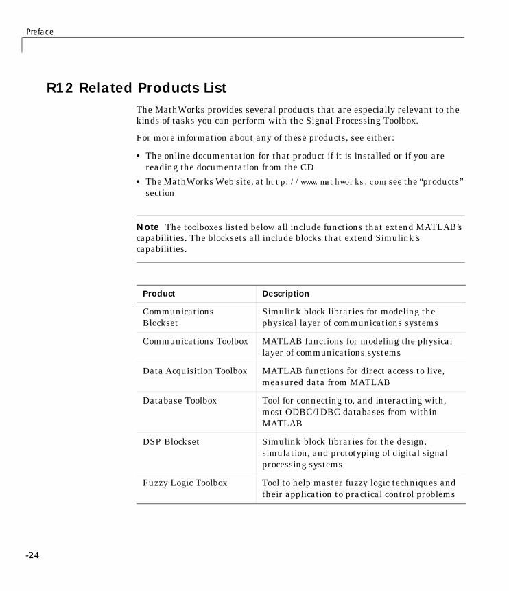
R12 Related Products ListThe MathWorks provides several products that are especially relevant to thekinds of tasks you can perform with the Signal Processing Toolbox.
For more information about any of these products, see either:
• The online documentation for that product if it is installed or if you arereading the documentation from the CD
• The MathWorks Web site, at http://www.mathworks.com; see the “products”section
Note The toolboxes listed below all include functions that extend MATLAB’scapabilities. The blocksets all include blocks that extend Simulink’scapabilities.
Product Description
CommunicationsBlockset
Simulink block libraries for modeling thephysical layer of communications systems
Communications Toolbox MATLAB functions for modeling the physicallayer of communications systems
Data Acquisition Toolbox MATLAB functions for direct access to live,measured data from MATLAB
Database Toolbox Tool for connecting to, and interacting with,most ODBC/JDBC databases from withinMATLAB
DSP Blockset Simulink block libraries for the design,simulation, and prototyping of digital signalprocessing systems
Fuzzy Logic Toolbox Tool to help master fuzzy logic techniques andtheir application to practical control problems
R12 Related Products List
-25
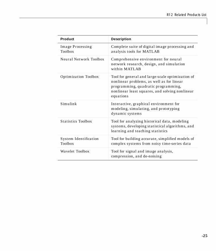
Image ProcessingToolbox
Complete suite of digital image processing andanalysis tools for MATLAB
Neural Network Toolbox Comprehensive environment for neuralnetwork research, design, and simulationwithin MATLAB
Optimization Toolbox Tool for general and large-scale optimization ofnonlinear problems, as well as for linearprogramming, quadratic programming,nonlinear least squares, and solving nonlinearequations
Simulink Interactive, graphical environment formodeling, simulating, and prototypingdynamic systems
Statistics Toolbox Tool for analyzing historical data, modelingsystems, developing statistical algorithms, andlearning and teaching statistics
System IdentificationToolbox
Tool for building accurate, simplified models ofcomplex systems from noisy time-series data
Wavelet Toolbox Tool for signal and image analysis,compression, and de-noising
Product Description

Preface
-26
How to Use This ManualThis section explains how to use the documentation to get help about the SignalProcessing Toolbox. Read the topic that best fits your skill level:
• “If You Are a New User”
• “If You Are an Experienced Toolbox User”
• “All Toolbox Users”
If You Are a New UserBegin with Chapter 1, “Signal Processing Basics.” This chapter introduces theMATLAB signal processing environment through the toolbox functions. Itdescribes the basic functions of the Signal Processing Toolbox, reviewing itsuse in basic waveform generation, filter implementation and analysis, impulseand frequency response, zero-pole analysis, linear system models, and thediscrete Fourier transform.
When you feel comfortable with the basic functions, move on to Chapter 2 andChapter 3 for a more in-depth introduction to using the Signal ProcessingToolbox:
• Chapter 2, “Filter Design,” for a detailed explanation of using the SignalProcessing Toolbox in infinite impulse response (IIR) and finite impulseresponse (FIR) filter design and implementation, including special topics inIIR filter design.
• Chapter 3, “Statistical Signal Processing,” for how to use the correlation,covariance, and spectral analysis tools to estimate important functions ofdiscrete random signals.
Once you understand the general principles and applications of the toolbox,learn how to use the interactive tools:
• Chapter 5, “Filter Design and Analysis Tool,” and Chapter 6, “SPTool: ASignal Processing GUI Suite,” for an overview of the interactive GUIenvironments and examples of how to use them for signal exploration, filterdesign and implementation, and spectral analysis.
Finally, see the following chapter:
How to Use This Manual
-27
• Chapter 4, “Special Topics,” for specialized functions, including filterwindows, parametric modeling, resampling, cepstrum analysis,time-dependent Fourier transforms and spectrograms, median filtering,communications applications, deconvolution, and specialized transforms.
If You Are an Experienced Toolbox UserSee Chapter 5, “Filter Design and Analysis Tool,” and Chapter 6, “SPTool: ASignal Processing GUI Suite,” for an overview of the interactive GUIenvironments and examples of how to use them for signal viewing, filter designand implementation, and spectral analysis.
All Toolbox UsersUse Chapter 7, “Function Reference,” for locating information on specificfunctions. Reference descriptions include a synopsis of the function’s syntax, aswell as a complete explanation of options and operations. Many referencedescriptions also include helpful examples, a description of the function’salgorithm, and references to additional reading material.
Use this manual in conjunction with the software to learn about the powerfulfeatures that MATLAB provides. Each chapter provides numerous examplesthat apply the toolbox to representative signal processing tasks.
Some examples use MATLAB’s random number generation function randn. Inthese cases, to duplicate the results in the example, type
randn('state',0)
before running the example.
Preface
-28
Installing the Signal Processing ToolboxTo determine if the Signal Processing Toolbox is installed on your system, typethis command at the MATLAB prompt.
ver
When you enter this command, MATLAB displays information about theversion of MATLAB you are running, including a list of all toolboxes installedon your system and their version numbers.
For information about installing the toolbox, see the MATLAB InstallationGuide for your platform.

Technical Conventions
-29
Technical ConventionsThis manual and the Signal Processing Toolbox functions use the followingtechnical notations.
Nyquist frequency One-half the sampling frequency. Sometoolbox functions normalize this value to 1.
x(1) The first element of a data sequence orfilter, corresponding to zero lag.
Ω or w Analog frequency in radians per second.
ω or w Digital frequency in radians per sample.
f Digital frequency in hertz.
[x, y) The interval from x to y, including x but notincluding y.
... Ellipses in the argument list for a givensyntax on a function reference pageindicate all possible argument lists for thatfunction appearing prior to the givensyntax are valid.
Preface
-30
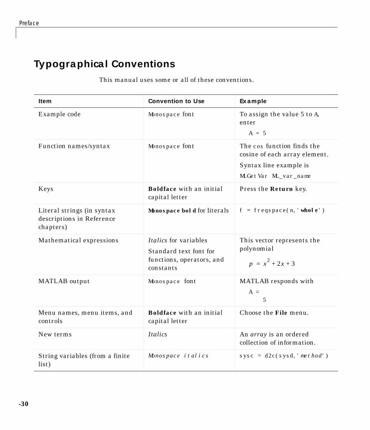
Typographical ConventionsThis manual uses some or all of these conventions.
Item Convention to Use Example
Example code Monospace font To assign the value 5 to A,enter
A = 5
Function names/syntax Monospace font The cos function finds thecosine of each array element.
Syntax line example is
MLGetVar ML_var_name
Keys Boldface with an initialcapital letter
Press the Return key.
Literal strings (in syntaxdescriptions in Referencechapters)
Monospace bold for literals f = freqspace(n,'whole')
Mathematical expressions Italics for variables
Standard text font forfunctions, operators, andconstants
This vector represents thepolynomial
MATLAB output Monospace font MATLAB responds with
A = 5
Menu names, menu items, andcontrols
Boldface with an initialcapital letter
Choose the File menu.
New terms Italics An array is an orderedcollection of information.
String variables (from a finitelist)
Monospace italics sysc = d2c(sysd,'method')
p x2 2x 3+ +=
1
Signal Processing Basics
Signal Processing Toolbox Central Features . . . . . 1-2
Representing Signals . . . . . . . . . . . . . . . . 1-4
Waveform Generation: Time Vectors and Sinusoids . . 1-6
Working with Data . . . . . . . . . . . . . . . . . 1-13
Filter Implementation and Analysis . . . . . . . . . 1-14
The filter Function . . . . . . . . . . . . . . . . . 1-17
Other Functions for Filtering . . . . . . . . . . . . 1-19
Impulse Response . . . . . . . . . . . . . . . . . 1-23
Frequency Response . . . . . . . . . . . . . . . . 1-24
Zero-Pole Analysis . . . . . . . . . . . . . . . . . 1-30
Linear System Models . . . . . . . . . . . . . . . 1-32
Discrete Fourier Transform . . . . . . . . . . . . . 1-44
Selected Bibliography . . . . . . . . . . . . . . . 1-47

1 Signal Processing Basics
1-2
OverviewThis chapter describes how to begin using MATLAB and the Signal ProcessingToolbox for your signal processing applications. It assumes a basic knowledgeand understanding of signals and systems, including such topics as filter andlinear system theory and basic Fourier analysis. The chapter covers thefollowing topics:
• “Signal Processing Toolbox Central Features”
• “Representing Signals”
• “Waveform Generation: Time Vectors and Sinusoids”
• “Working with Data”
• “Filter Implementation and Analysis”
• “The filter Function”
• “Other Functions for Filtering”
• “Impulse Response”
• “Frequency Response”
• “Zero-Pole Analysis”
• “Linear System Models”
• “Discrete Fourier Transform”
• “Selected Bibliography”
Many examples throughout the chapter demonstrate how to apply toolboxfunctions. If you are not already familiar with MATLAB’s signal processingcapabilities, use this chapter in conjunction with the software to try examplesand learn about the powerful features available to you.
Signal Processing Toolbox Central Features
1-3
Signal Processing Toolbox Central FeaturesThe Signal Processing Toolbox functions are algorithms, expressed mostly inM-files, that implement a variety of signal processing tasks. These toolboxfunctions are a specialized extension of the MATLAB computational andgraphical environment.
Filtering and FFTsTwo of the most important functions for signal processing are not in the SignalProcessing Toolbox at all, but are built-in MATLAB functions:
• filter applies a digital filter to a data sequence.
• fft calculates the discrete Fourier transform of a sequence.
The operations these functions perform are the main computationalworkhorses of classical signal processing. Both are described in this chapter.The Signal Processing Toolbox uses many other standard MATLAB functionsand language features, including polynomial root finding, complex arithmetic,matrix inversion and manipulation, and graphics tools.
Signals and SystemsThe basic entities that toolbox functions work with are signals and systems.The functions emphasize digital, or discrete, signals and filters, as opposed toanalog, or continuous, signals. The principal filter type the toolbox supports isthe linear, time-invariant digital filter with a single input and a single output.You can represent linear time-invariant systems using one of several models(such as transfer function, state-space, zero-pole-gain, and second-ordersection) and convert between representations.
Key Areas: Filter Design and Spectral AnalysisIn addition to its core functions, the toolbox provides rich, customizable supportfor the key areas of filter design and spectral analysis. It is easy to implementa design technique that suits your application, design digital filters directly, orcreate analog prototypes and discretize them. Toolbox functions also estimatepower spectral density and cross spectral density, using either parametric ornonparametric techniques. “Filter Design” on page 2-1 and “Statistical SignalProcessing” on page 3-1 respectively detail toolbox functions for filter designand spectral analysis.
1 Signal Processing Basics
1-4
There are functions for computation and graphical display of frequencyresponse, as well as functions for system identification; generating signals;discrete cosine, chirp-z, and Hilbert transforms; lattice filters; resampling;time-frequency analysis; and basic communication systems simulation.
Interactive Tools: SPTool and FDAToolThe power of the Signal Processing Toolbox is greatly enhanced by itseasy-to-use interactive tools. SPTool provides a rich graphical environment forsignal viewing, filter design, and spectral analysis. The Filter Design andAnalysis Tool (FDATool) provides a more comprehensive collection of featuresfor addressing the problem of filter design. The FDATool also offers seamlessaccess to the additional filter design methods and quantization features of theFilter Design Toolbox when that product is installed.
ExtensibilityPerhaps the most important feature of the MATLAB environment is that it isextensible: MATLAB lets you create your own M-files to meet numericcomputation needs for research, design, or engineering of signal processingsystems. Simply copy the M-files provided with the Signal Processing Toolboxand modify them as needed, or create new functions to expand the functionalityof the toolbox.
Representing Signals
1-5
Representing SignalsThe central data construct in MATLAB is the numeric array, an orderedcollection of real or complex numeric data with two or more dimensions. Thebasic data objects of signal processing (one-dimensional signals or sequences,multichannel signals, and two-dimensional signals) are all naturally suited toarray representation.
Vector RepresentationMATLAB represents ordinary one-dimensional sampled data signals, orsequences, as vectors. Vectors are 1-by-n or n-by-1 arrays, where n is thenumber of samples in the sequence. One way to introduce a sequence intoMATLAB is to enter it as a list of elements at the command prompt. Thestatement
x = [4 3 7 -9 1]
creates a simple five-element real sequence in a row vector. Transpositionturns the sequence into a column vector
x = x'
resulting in
x =437-91
Column orientation is preferable for single channel signals because it extendsnaturally to the multichannel case. For multichannel data, each column of amatrix represents one channel. Each row of such a matrix then corresponds toa sample point. A three-channel signal that consists of x, 2x, and x/π is
y = [x 2*x x/pi]

1 Signal Processing Basics
1-6
This results in
y =4.0000 8.0000 1.27323.0000 6.0000 0.95497.0000 14.0000 2.2282-9.0000 -18.0000 -2.86481.0000 2.0000 0.3183

Waveform Generation: Time Vectors and Sinusoids
1-7
Waveform Generation: Time Vectors and SinusoidsA variety of toolbox functions generate waveforms. Most require you to beginwith a vector representing a time base. Consider generating data with a 1000Hz sample frequency, for example. An appropriate time vector is
t = (0:0.001:1)';
where MATLAB’s colon operator creates a 1001-element row vector thatrepresents time running from zero to one second in steps of one millisecond.The transpose operator (') changes the row vector into a column; thesemicolon (;) tells MATLAB to compute but not display the result.
Given t you can create a sample signal y consisting of two sinusoids, one at 50Hz and one at 120 Hz with twice the amplitude.
y = sin(2*pi*50*t) + 2*sin(2*pi*120*t);
The new variable y, formed from vector t, is also 1001 elements long. You canadd normally distributed white noise to the signal and graph the first fiftypoints using
randn('state',0);yn = y + 0.5*randn(size(t));plot(t(1:50),yn(1:50))
0 0.01 0.02 0.03 0.04 0.05−3
−2
−1
0
1
2
3
4
1 Signal Processing Basics
1-8
Common Sequences: Unit Impulse, Unit Step, and Unit RampSince MATLAB is a programming language, an endless variety of differentsignals is possible. Here are some statements that generate several commonlyused sequences, including the unit impulse, unit step, and unit ramp functions.
t = (0:0.001:1)';y = [1; zeros(99,1)]; % impulsey = ones(100,1); % step (filter assumes 0 initial cond.)y = t; % rampy = t.^2;y = square(4*t);
All of these sequences are column vectors. The last three inherit their shapesfrom t.
Multichannel SignalsUse standard MATLAB array syntax to work with multichannel signals. Forexample, a multichannel signal consisting of the last three signals generatedabove is
z = [t t.^2 square(4*t)];
You can generate a multichannel unit sample function using the outer productoperator. For example, a six-element column vector whose first element is one,and whose remaining five elements are zeros, is
a = [1 zeros(1,5)]';
To duplicate column vector a into a matrix without performing anymultiplication, use MATLAB’s colon operator and the ones function.
c = a(:,ones(1,3));

Waveform Generation: Time Vectors and Sinusoids
1-9
Common Periodic WaveformsThe toolbox provides functions for generating widely used periodic waveforms:
• sawtooth generates a sawtooth wave with peaks at ±1 and a period of . Anoptional width parameter specifies a fractional multiple of at which thesignal’s maximum occurs.
• square generates a square wave with a period of . An optional parameterspecifies duty cycle, the percent of the period for which the signal is positive.
To generate 1.5 seconds of a 50 Hz sawtooth wave with a sample rate of 10 kHzand plot 0.2 seconds of the generated waveform, use
fs = 10000;t = 0:1/fs:1.5;x = sawtooth(2*pi*50*t);plot(t,x), axis([0 0.2 -1 1])
2π2π
2π
0 0.02 0.04 0.06 0.08 0.1 0.12 0.14 0.16 0.18 0.2-1
-0.5
0
0.5
1
1 Signal Processing Basics
1-10
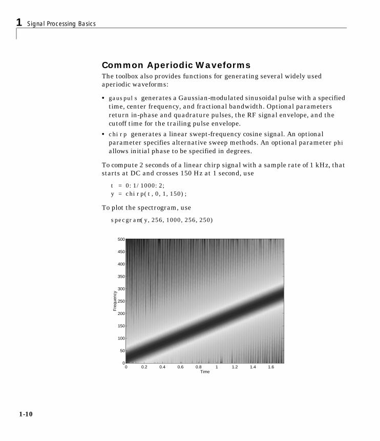
Common Aperiodic WaveformsThe toolbox also provides functions for generating several widely usedaperiodic waveforms:
• gauspuls generates a Gaussian-modulated sinusoidal pulse with a specifiedtime, center frequency, and fractional bandwidth. Optional parametersreturn in-phase and quadrature pulses, the RF signal envelope, and thecutoff time for the trailing pulse envelope.
• chirp generates a linear swept-frequency cosine signal. An optionalparameter specifies alternative sweep methods. An optional parameter phiallows initial phase to be specified in degrees.
To compute 2 seconds of a linear chirp signal with a sample rate of 1 kHz, thatstarts at DC and crosses 150 Hz at 1 second, use
t = 0:1/1000:2;y = chirp(t,0,1,150);
To plot the spectrogram, use
specgram(y,256,1000,256,250)
Time
Fre
quen
cy
0 0.2 0.4 0.6 0.8 1 1.2 1.4 1.60
50
100
150
200
250
300
350
400
450
500

Waveform Generation: Time Vectors and Sinusoids
1-11
The pulstran FunctionThe pulstran function generates pulse trains from either continuous orsampled prototype pulses. The following example generates a pulse trainconsisting of the sum of multiple delayed interpolations of a Gaussian pulse.The pulse train is defined to have a sample rate of 50 kHz, a pulse train lengthof 10 ms, and a pulse repetition rate of 1 kHz; D specifies the delay to each pulserepetition in column 1 and an optional attenuation for each repetition incolumn 2. The pulse train is constructed by passing the name of the gauspulsfunction to pulstran, along with additional parameters that specify a 10 kHzGaussian pulse with 50% bandwidth.
T = 0:1/50E3:10E-3;D = [0:1/1E3:10E-3;0.8.^(0:10)]';Y = pulstran(T,D,'gauspuls',10E3,0.5);plot(T,Y)
0 0.001 0.002 0.003 0.004 0.005 0.006 0.007 0.008 0.009 0.01-0.8
-0.6
-0.4
-0.2
0
0.2
0.4
0.6
0.8
1

1 Signal Processing Basics
1-12
The Sinc FunctionThe sinc function computes the mathematical sinc function for an input vectoror matrix x. The sinc function is the continuous inverse Fourier transform ofthe rectangular pulse of width and height 1.
The sinc function has a value of 1 where x is zero, and a value of
for all other elements of x.
To plot the sinc function for a linearly spaced vector with values ranging from-5 to 5, use the following commands.
x = linspace(-5,5);y = sinc(x);plot(x,y)
2π
πx( )sinπx
--------------------
-5 -4 -3 -2 -1 0 1 2 3 4 5-0.4
-0.2
0
0.2
0.4
0.6
0.8
1
Waveform Generation: Time Vectors and Sinusoids
1-13
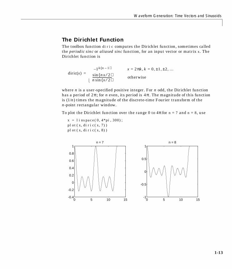
The Dirichlet FunctionThe toolbox function diric computes the Dirichlet function, sometimes calledthe periodic sinc or aliased sinc function, for an input vector or matrix x. TheDirichlet function is
where n is a user-specified positive integer. For n odd, the Dirichlet functionhas a period of ; for n even, its period is . The magnitude of this functionis (1/n) times the magnitude of the discrete-time Fourier transform of then-point rectangular window.
To plot the Dirichlet function over the range 0 to 4π for n = 7 and n = 8, use
x = linspace(0,4*pi,300);plot(x,diric(x,7))plot(x,diric(x,8))
diric x( )1– k n 1–( ) x 2πk k 0 1± 2± …, , ,=,=
nx 2⁄( )sinn x 2⁄( )sin---------------------------- otherwise
=
2π 4π
0 5 10 15-0.4
-0.2
0
0.2
0.4
0.6
0.8
1n = 7
0 5 10 15-1
-0.5
0
0.5
1n = 8

1 Signal Processing Basics
1-14
Working with DataThe examples in the preceding sections obtain data in one of two ways:
• By direct input, that is, entering the data manually at the keyboard
• By using a MATLAB or toolbox function, such as sin, cos, sawtooth, square,or sinc
Some applications, however, may need to import data from outside MATLAB.Depending on your data format, you can do this in the following ways:
• Load data from an ASCII file or MAT-file with MATLAB’s load command.
• Read the data into MATLAB with a low-level file I/O function, such as fopen,fread, and fscanf.
• Develop a MEX-file to read the data.
Other resources are also useful, such as a high-level language program (inFortran or C, for example) that converts your data into MAT-file format – seethe “MATLAB External Interfaces/API Reference” for details. MATLAB readssuch files using the load command.
Similar techniques are available for exporting data generated withinMATLAB. See the MATLAB documentation for more details on importing andexporting data.
Filter Implementation and Analysis
1-15
Filter Implementation and AnalysisThis section describes how to filter discrete signals using MATLAB’s filterfunction and other functions in the Signal Processing Toolbox. It also discusseshow to use the toolbox functions to analyze filter characteristics, includingimpulse response, magnitude and phase response, group delay, and zero-polelocations.
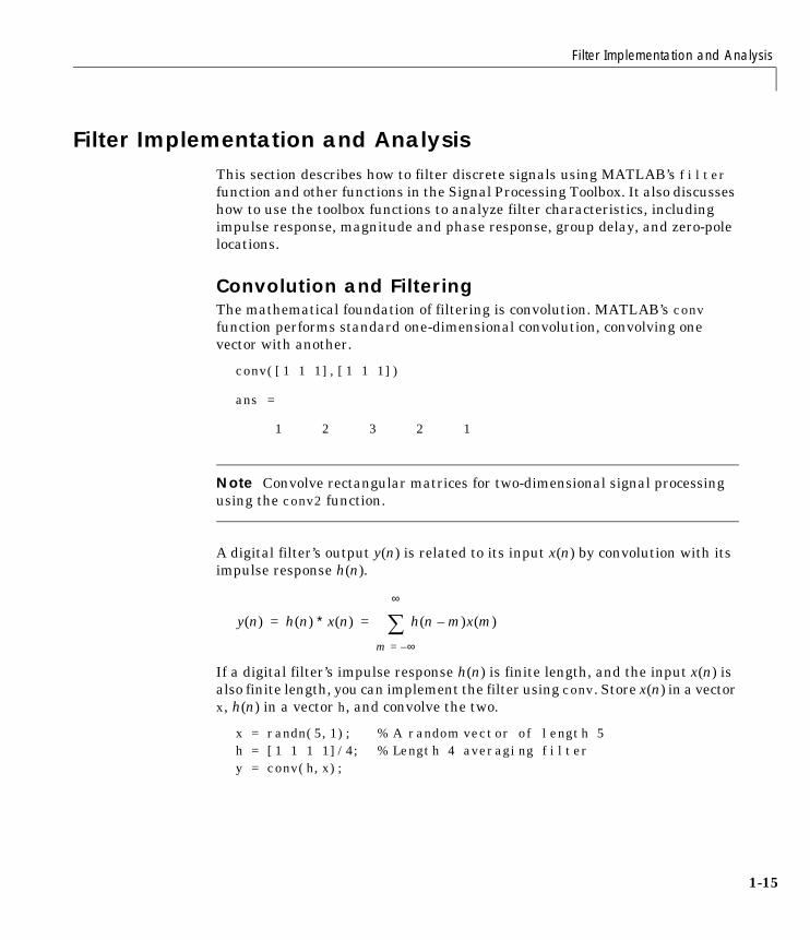
Convolution and FilteringThe mathematical foundation of filtering is convolution. MATLAB’s convfunction performs standard one-dimensional convolution, convolving onevector with another.
conv([1 1 1],[1 1 1])
ans =
1 2 3 2 1
Note Convolve rectangular matrices for two-dimensional signal processingusing the conv2 function.
A digital filter’s output y(n) is related to its input x(n) by convolution with itsimpulse response h(n).
If a digital filter’s impulse response h(n) is finite length, and the input x(n) isalso finite length, you can implement the filter using conv. Store x(n) in a vectorx, h(n) in a vector h, and convolve the two.
x = randn(5,1); % A random vector of length 5h = [1 1 1 1]/4; % Length 4 averaging filtery = conv(h,x);
y n( ) h n( ) x n( )∗ h n m–( )x m( )
m ∞–=
∞
= =
1 Signal Processing Basics
1-16
Filters and Transfer FunctionsIn general, the z-transform Y(z) of a digital filter’s output y(n) is related to thez-transform X(z) of the input by
where H(z) is the filter’s transfer function. Here, the constants b(i) and a(i) arethe filter coefficients and the order of the filter is the maximum of na and nb.
Note The filter coefficients start with subscript 1, rather than 0. This reflectsMATLAB’s standard indexing scheme for vectors.
MATLAB stores the coefficients in two vectors, one for the numerator and onefor the denominator. By convention, MATLAB uses row vectors for filtercoefficients.
Filter Coefficients and Filter NamesMany standard names for filters reflect the number of a and b coefficientspresent:
• When nb = 0 (that is, b is a scalar), the filter is an Infinite Impulse Response(IIR), all-pole, recursive, or autoregressive (AR) filter.
• When na = 0 (that is, a is a scalar), the filter is a Finite Impulse Response(FIR), all-zero, nonrecursive, or moving average (MA) filter.
• If both na and nb are greater than zero, the filter is an IIR, pole-zero,recursive, or autoregressive moving average (ARMA) filter.
The acronyms AR, MA, and ARMA are usually applied to filters associatedwith filtered stochastic processes.
Y z( ) H z( )X z( )b 1( ) b 2( )z 1– b nb 1+( )z nb–+ + +a 1( ) a 2( )z 1– a na 1+( )z na–+ + +--------------------------------------------------------------------------------------------X z( )= =
Filter Implementation and Analysis
1-17
Filtering with the filter FunctionIt is simple to work back to a difference equation from the z-transform relationshown earlier. Assume that a(1) = 1. Move the denominator to the left-handside and take the inverse z-transform.
In terms of current and past inputs, and past outputs, y(n) is
This is the standard time-domain representation of a digital filter, computedstarting with y(1) and assuming zero initial conditions. This representation’sprogression is
A filter in this form is easy to implement with the filter function. Forexample, a simple single-pole filter (lowpass) is
b = 1; % Numeratora = [1 -0.9]; % Denominator
where the vectors b and a represent the coefficients of a filter in transferfunction form. To apply this filter to your data, use
y = filter(b,a,x);
filter gives you as many output samples as there are input samples, that is,the length of y is the same as the length of x. If the first element of a is not 1,filter divides the coefficients by a(1) before implementing the differenceequation.
y n( ) a2y n 1–( ) ana 1+ y n na–( )+ + + b1x n( ) b2x n 1–( ) bnb 1+ x n nb–( )+ + +=
y n( ) b1x n( ) b2x n 1–( ) bnb 1+ x n nb–( ) a2y n 1–( ) – ana 1+ y n na–( )––+ + +=
y 1( ) b1x 1( )=
y 2( ) b1x 2( ) b2x 1( ) a2y 1( )–+=
y 3( ) b1x 3( ) b2x 2( ) b3x 1( ) a2y 2( ) a3y 1( )––+ +=
=
1 Signal Processing Basics
1-18
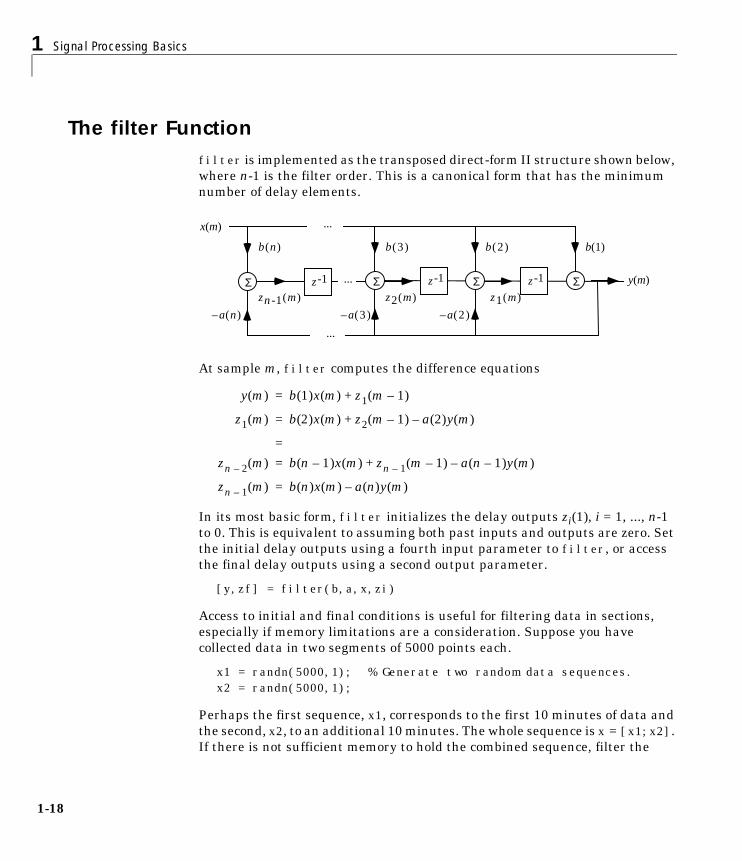
The filter Function filter is implemented as the transposed direct-form II structure shown below,where n-1 is the filter order. This is a canonical form that has the minimumnumber of delay elements.
At sample m, filter computes the difference equations
In its most basic form, filter initializes the delay outputs zi(1), i = 1, ..., n-1to 0. This is equivalent to assuming both past inputs and outputs are zero. Setthe initial delay outputs using a fourth input parameter to filter, or accessthe final delay outputs using a second output parameter.
[y,zf] = filter(b,a,x,zi)
Access to initial and final conditions is useful for filtering data in sections,especially if memory limitations are a consideration. Suppose you havecollected data in two segments of 5000 points each.
x1 = randn(5000,1); % Generate two random data sequences.x2 = randn(5000,1);
Perhaps the first sequence, x1, corresponds to the first 10 minutes of data andthe second, x2, to an additional 10 minutes. The whole sequence is x = [x1;x2].If there is not sufficient memory to hold the combined sequence, filter the
Σ Σ Σz -1 z -1
x(m)
y(m)
b(3) b(2) b(1)
–a(3) –a(2)
z1(m)z2(m)Σ z -1
b(n)
–a(n)
zn -1(m)
...
...
...
y m( ) b 1( )x m( ) z1 m 1–( )+=
z1 m( ) b 2( )x m( ) z2 m 1–( ) a 2( )y m( )–+=
=
zn 2– m( ) b n 1–( )x m( ) zn 1– m 1–( ) a n 1–( )y m( )–+=
zn 1– m( ) b n( )x m( ) a n( )y m( )–=
The filter Function
1-19
subsequences x1 and x2 one at a time. To ensure continuity of the filteredsequences, use the final conditions from x1 as initial conditions to filter x2.
[y1,zf] = filter(b,a,x1);y2 = filter(b,a,x2,zf);
The filtic function generates initial conditions for filter. filtic computesthe delay vector to make the behavior of the filter reflect past inputs andoutputs that you specify. To obtain the same output delay values zf as aboveusing filtic, use
zf = filtic(b,a,flipud(y1),flipud(x1));
This can be useful when filtering short data sequences, as appropriate initialconditions help reduce transient startup effects.
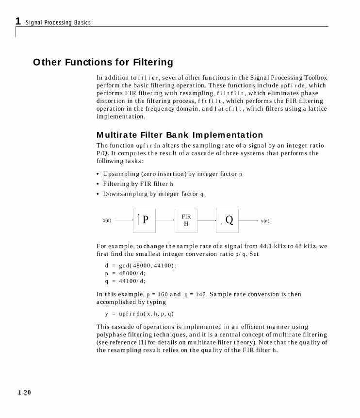
1 Signal Processing Basics
1-20
Other Functions for FilteringIn addition to filter, several other functions in the Signal Processing Toolboxperform the basic filtering operation. These functions include upfirdn, whichperforms FIR filtering with resampling, filtfilt, which eliminates phasedistortion in the filtering process, fftfilt, which performs the FIR filteringoperation in the frequency domain, and latcfilt, which filters using a latticeimplementation.
Multirate Filter Bank ImplementationThe function upfirdn alters the sampling rate of a signal by an integer ratioP/Q. It computes the result of a cascade of three systems that performs thefollowing tasks:
• Upsampling (zero insertion) by integer factor p
• Filtering by FIR filter h
• Downsampling by integer factor q
For example, to change the sample rate of a signal from 44.1 kHz to 48 kHz, wefirst find the smallest integer conversion ratio p/q. Set
d = gcd(48000,44100);p = 48000/d;q = 44100/d;
In this example, p = 160 and q = 147. Sample rate conversion is thenaccomplished by typing
y = upfirdn(x,h,p,q)
This cascade of operations is implemented in an efficient manner usingpolyphase filtering techniques, and it is a central concept of multirate filtering(see reference [1] for details on multirate filter theory). Note that the quality ofthe resampling result relies on the quality of the FIR filter h.
Px(n) y(n)FIRH Q

Other Functions for Filtering
1-21
Filter banks may be implemented using upfirdn by allowing the filter h to bea matrix, with one FIR filter per column. A signal vector is passedindependently through each FIR filter, resulting in a matrix of output signals.
Other functions that perform multirate filtering (with fixed filter) includeresample, interp, and decimate.
Anti-Causal, Zero-Phase Filter ImplementationIn the case of FIR filters, it is possible to design linear phase filters that, whenapplied to data (using filter or conv), simply delay the output by a fixednumber of samples. For IIR filters, however, the phase distortion is usuallyhighly nonlinear. The filtfilt function uses the information in the signal atpoints before and after the current point, in essence “looking into the future,”to eliminate phase distortion.
To see how filtfilt does this, recall that if the z-transform of a real sequencex(n) is X(z), the z-transform of the time reversed sequence x(n) is X(1/z).Consider the processing scheme
When |z| = 1, that is z = ejω, the output reduces to X(ejω)|H(ejω)|2. Given allthe samples of the sequence x(n), a doubly filtered version of x that haszero-phase distortion is possible.
For example, a 1-second duration signal sampled at 100 Hz, composed of twosinusoidal components at 3 Hz and 40 Hz, is
fs = 100;t = 0:1/fs:1;x = sin(2*pi*t*3)+.25*sin(2*pi*t*40);
H(z)X(z)
X(z)H(z) X(1/z)H(1/z) X(1/z)H(1/z)H(z)
X(z)H(1/z)H(z)H(z)TimeReverse
TimeReverse

1 Signal Processing Basics
1-22
Now create a 10-point averaging FIR filter, and filter x using both filter andfiltfilt for comparison.
b = ones(1,10)/10; % 10 point averaging filtery = filtfilt(b,1,x); % Noncausal filteringyy = filter(b,1,x); % Normal filteringplot(t,x,t,y,'--',t,yy,':')
Both filtered versions eliminate the 40 Hz sinusoid evident in the original,solid line. The plot also shows how filter and filtfilt differ; the dashed(filtfilt) line is in phase with the original 3 Hz sinusoid, while the dotted(filter) line is delayed by about five samples. Also, the amplitude of thedashed line is smaller due to the magnitude squared effects of filtfilt.
filtfilt reduces filter startup transients by carefully choosing initialconditions, and by prepending onto the input sequence a short, reflected pieceof the input sequence. For best results, make sure the sequence you arefiltering has length at least three times the filter order and tapers to zero onboth edges.
0 0.1 0.2 0.3 0.4 0.5 0.6 0.7 0.8 0.9 1-1.5
-1
-0.5
0
0.5
1
1.5
Other Functions for Filtering
1-23
Frequency Domain Filter ImplementationDuality between the time domain and the frequency domain makes it possibleto perform any operation in either domain. Usually one domain or the other ismore convenient for a particular operation, but you can always accomplish agiven operation in either domain.
To implement general IIR filtering in the frequency domain, multiply thediscrete Fourier transform (DFT) of the input sequence with the quotient of theDFT of the filter.
n = length(x);y = ifft(fft(x).*fft(b,n)./fft(a,n));
This computes results that are identical to filter, but with different startuptransients (edge effects). For long sequences, this computation is veryinefficient because of the large zero-padded FFT operations on the filtercoefficients, and because the FFT algorithm becomes less efficient as thenumber of points n increases.
For FIR filters, however, it is possible to break longer sequences into shorter,computationally efficient FFT lengths. The function
y = fftfilt(b,x)
uses the overlap add method (see reference [1] at the end of this chapter) tofilter a long sequence with multiple medium-length FFTs. Its output isequivalent to filter(b,1,x).

1 Signal Processing Basics
1-24
Impulse ResponseThe impulse response of a digital filter is the output arising from the unitimpulse input sequence defined as
In MATLAB, you can generate an impulse sequence a number of ways; onestraightforward way is
imp = [1; zeros(49,1)];
The impulse response of the simple filter b = 1 and a = [1 -0.9] is
h = filter(b,a,imp);
The impz function in the toolbox simplifies this operation, choosing the numberof points to generate and then making a stem plot (using the stem function).
impz(b,a)
The plot shows the exponential decay h(n) = 0.9n of the single pole system.
x n( )1 n 1=,0 n 1≠,
=
0 10 20 30 40 50 60 70 80 900
0.1
0.2
0.3
0.4
0.5
0.6
0.7
0.8
0.9
1
Frequency Response
1-25
Frequency ResponseThe Signal Processing Toolbox enables you to perform frequency domainanalysis of both analog and digital filters.
Digital Domainfreqz uses an FFT-based algorithm to calculate the z-transform frequencyresponse of a digital filter. Specifically, the statement
[h,w] = freqz(b,a,n)
returns the n-point complex frequency response, , of the digital filter.
In its simplest form, freqz accepts the filter coefficient vectors b and a, and aninteger n specifying the number of points at which to calculate the frequencyresponse. freqz returns the complex frequency response in vector h, and theactual frequency points in vector w in rad/s.
freqz can accept other parameters, such as a sampling frequency or a vector ofarbitrary frequency points. The example below finds the 256-point frequencyresponse for a 12th-order Chebyshev type I filter. The call to freqz specifies asampling frequency fs of 1000 Hz.
[b,a] = cheby1(12,0.5,200/500);[h,f] = freqz(b,a,256,1000);
Because the parameter list includes a sampling frequency, freqz returns avector f that contains the 256 frequency points between 0 and fs/2 used in thefrequency response calculation.
H ejω( )
H ejω( )b 1( ) b 2( )e j– ω b nb 1+( )e j– ω nb( )+ + +
a 1( ) a 2( )e j– ω a na 1+( )e j– ω na( )+ + +-------------------------------------------------------------------------------------------------------=
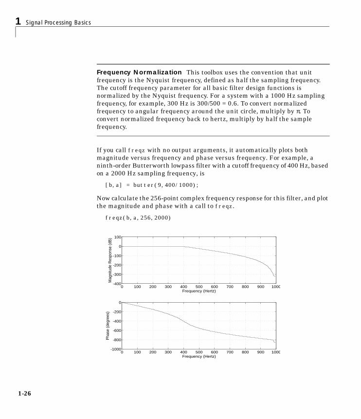
1 Signal Processing Basics
1-26
Frequency Normalization This toolbox uses the convention that unitfrequency is the Nyquist frequency, defined as half the sampling frequency.The cutoff frequency parameter for all basic filter design functions isnormalized by the Nyquist frequency. For a system with a 1000 Hz samplingfrequency, for example, 300 Hz is 300/500 = 0.6. To convert normalizedfrequency to angular frequency around the unit circle, multiply by π. Toconvert normalized frequency back to hertz, multiply by half the samplefrequency.
If you call freqz with no output arguments, it automatically plots bothmagnitude versus frequency and phase versus frequency. For example, aninth-order Butterworth lowpass filter with a cutoff frequency of 400 Hz, basedon a 2000 Hz sampling frequency, is
[b,a] = butter(9,400/1000);
Now calculate the 256-point complex frequency response for this filter, and plotthe magnitude and phase with a call to freqz.
freqz(b,a,256,2000)
0 100 200 300 400 500 600 700 800 900 1000-1000
-800
-600
-400
-200
0
Frequency (Hertz)
Pha
se (d
egre
es)
0 100 200 300 400 500 600 700 800 900 1000-400
-300
-200
-100
0
100
Frequency (Hertz)
Mag
nitu
de R
espo
nse
(dB
)
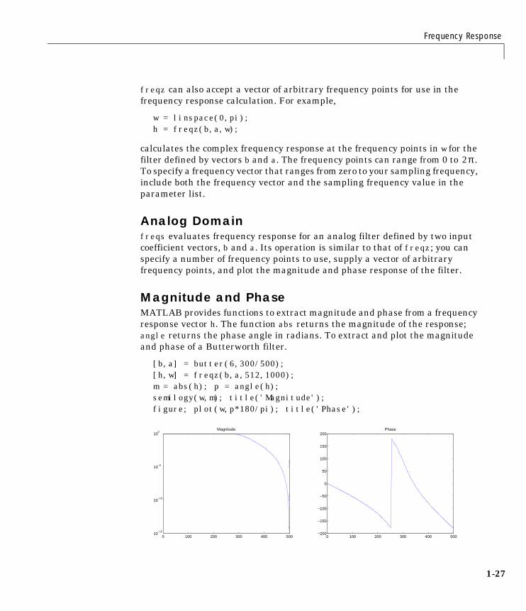
Frequency Response
1-27
freqz can also accept a vector of arbitrary frequency points for use in thefrequency response calculation. For example,
w = linspace(0,pi);h = freqz(b,a,w);
calculates the complex frequency response at the frequency points in w for thefilter defined by vectors b and a. The frequency points can range from 0 to .To specify a frequency vector that ranges from zero to your sampling frequency,include both the frequency vector and the sampling frequency value in theparameter list.
Analog Domainfreqs evaluates frequency response for an analog filter defined by two inputcoefficient vectors, b and a. Its operation is similar to that of freqz; you canspecify a number of frequency points to use, supply a vector of arbitraryfrequency points, and plot the magnitude and phase response of the filter.
Magnitude and PhaseMATLAB provides functions to extract magnitude and phase from a frequencyresponse vector h. The function abs returns the magnitude of the response;angle returns the phase angle in radians. To extract and plot the magnitudeand phase of a Butterworth filter.
[b,a] = butter(6,300/500);[h,w] = freqz(b,a,512,1000);m = abs(h); p = angle(h);semilogy(w,m); title('Magnitude');figure; plot(w,p*180/pi); title('Phase');
2π
0 100 200 300 400 50010
−15
10−10
10−5
100
Magnitude
0 100 200 300 400 500−200
−150
−100
−50
0
50
100
150
200Phase

1 Signal Processing Basics
1-28
The unwrap function is also useful in frequency analysis. unwrap unwraps thephase to make it continuous across 360° phase discontinuities by addingmultiples of ±360°, as needed. To see how unwrap is useful, design a 25th-orderlowpass FIR filter.
h = fir1(25,0.4);
Obtain the filter’s frequency response with freqz, and plot the phase indegrees.
[H,f] = freqz(h,1,512,2);plot(f,angle(H)*180/pi); grid
It is difficult to distinguish the 360° jumps (an artifact of the arctangentfunction inside angle) from the 180° jumps that signify zeros in the frequencyresponse.
Use unwrap to eliminate the 360° jumps.
plot(f,unwrap(angle(H))*180/pi); grid
0 0.1 0.2 0.3 0.4 0.5 0.6 0.7 0.8 0.9 1-200
-150
-100
-50
0
50
100
150
200
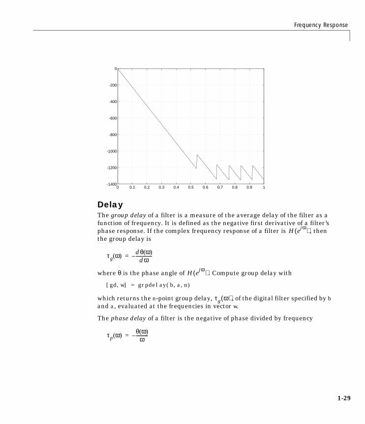
Frequency Response
1-29
DelayThe group delay of a filter is a measure of the average delay of the filter as afunction of frequency. It is defined as the negative first derivative of a filter’sphase response. If the complex frequency response of a filter is , thenthe group delay is
where θ is the phase angle of . Compute group delay with
[gd,w] = grpdelay(b,a,n)
which returns the n-point group delay, , of the digital filter specified by band a, evaluated at the frequencies in vector w.
The phase delay of a filter is the negative of phase divided by frequency
0 0.1 0.2 0.3 0.4 0.5 0.6 0.7 0.8 0.9 1-1400
-1200
-1000
-800
-600
-400
-200
0
H ejω( )
τg ω( )dθ ω( )
dω---------------–=
H ejω( )
τg ω( )
τp ω( )θ ω( )
ω-----------–=

1 Signal Processing Basics
1-30
To plot both the group and phase delays of a system on the same graph, type
[b,a] = butter(10,200/1000);gd = grpdelay(b,a,128);[h,f] = freqz(b,a,128,2000);pd = -unwrap(angle(h))*(2000/(2*pi))./f;plot(f,gd,'-',f,pd,'--')axis([0 1000 -30 30])legend('Group Delay','Phase Delay')
0 200 400 600 800 1000−30
−20
−10
0
10
20
30Group DelayPhase Delay

Zero-Pole Analysis
1-31
Zero-Pole AnalysisThe zplane function plots poles and zeros of a linear system. For example, asimple filter with a zero at -1/2 and a complex pole pair at and
is
zer = -0.5; pol = 0.9*exp(j*2*pi*[-0.3 0.3]');
The zero-pole plot for the filter is
zplane(zer,pol)
For a system in zero-pole form, supply column vector arguments z and p tozplane.
zplane(z,p)
For a system in transfer function form, supply row vectors b and a asarguments to zplane.
zplane(b,a)
0.9ej2π 0.3( )
0.9e j– 2π 0.3( )
-1 -0.5 0 0.5 1
-1
-0.8
-0.6
-0.4
-0.2
0
0.2
0.4
0.6
0.8
1
Real part
Imag
inar
y pa
rt

1 Signal Processing Basics
1-32
In this case zplane finds the roots of b and a using the roots function and plotsthe resulting zeros and poles.
See “Linear System Models” on page 1-33 for details on zero-pole and transferfunction representation of systems.
Linear System Models
1-33
Linear System ModelsThe Signal Processing Toolbox provides several models for representing lineartime-invariant systems. This flexibility lets you choose the representationalscheme that best suits your application and, within the bounds of numericstability, convert freely to and from most other models. This section provides abrief overview of supported linear system models and describes how to workwith these models in MATLAB.
Discrete-Time System ModelsThe discrete-time system models are representational schemes for digitalfilters. MATLAB supports several discrete-time system models, which aredescribed in the following sections:
• “Transfer Function”
• “Zero-Pole-Gain”
• “State-Space”
• “Partial Fraction Expansion (Residue Form)”
• “Second-Order Sections (SOS)”
• “Lattice Structure”
• “Convolution Matrix”
Transfer FunctionThe transfer function is a basic z-domain representation of a digital filter,expressing the filter as a ratio of two polynomials. It is the principaldiscrete-time model for this toolbox. The transfer function model descriptionfor the z-transform of a digital filter’s difference equation is
Here, the constants b(i) and a(i) are the filter coefficients, and the order of thefilter is the maximum of na and nb. In MATLAB, you store these coefficients intwo vectors (row vectors by convention), one row vector for the numerator andone for the denominator. See “Filters and Transfer Functions” on page 1-16 formore details on the transfer function form.
Y z( )b 1( ) b 2( )z 1– b nb 1+( )z nb–+ + +a 1( ) a 2( )z 1– a na 1+( )z na–+ + +--------------------------------------------------------------------------------------------X z( )=
1 Signal Processing Basics
1-34
Zero-Pole-GainThe factored or zero-pole-gain form of a transfer function is
By convention, MATLAB stores polynomial coefficients in row vectors andpolynomial roots in column vectors. In zero-pole-gain form, therefore, the zeroand pole locations for the numerator and denominator of a transfer functionreside in column vectors. The factored transfer function gain k is a MATLABscalar.
The poly and roots functions convert between polynomial and zero-pole-gainrepresentations. For example, a simple IIR filter is
b = [2 3 4];a = [1 3 3 1];
The zeros and poles of this filter are
q = roots(b)
q =-0.7500 + 1.1990i-0.7500 - 1.1990i
p = roots(a)
p =-1.0000-1.0000 + 0.0000i-1.0000 - 0.0000i
k = b(1)/a(1)
k =2
Returning to the original polynomials,
bb = k*poly(q)
bb =2.0000 3.0000 4.0000
H z( )q z( )p z( )---------- k z q 1( )–( ) z q 2( )–( ) z q n( )–( )
z p 1( )–( ) z p 2( )–( ) z p n( )–( )--------------------------------------------------------------------------------= =
Linear System Models
1-35
aa = poly(p)
aa =1.0000 3.0000 3.0000 1.0000
Note that b and a in this case represent the transfer function
For b = [2 3 4], the roots function misses the zero for z equal to 0. In fact, itmisses poles and zeros for z equal to 0 whenever the input transfer function hasmore poles than zeros, or vice versa. This is acceptable in most cases. Tocircumvent the problem, however, simply append zeros to make the vectors thesame length before using the roots function; for example, b = [b 0].
State-SpaceIt is always possible to represent a digital filter, or a system of differenceequations, as a set of first-order difference equations. In matrix or state-spaceform, you can write the equations as
where u is the input, x is the state vector, and y is the output. Forsingle-channel systems, A is an m-by-m matrix where m is the order of the filter,B is a column vector, C is a row vector, and D is a scalar. State-space notation isespecially convenient for multichannel systems where input u and output ybecome vectors, and B, C, and D become matrices.
State-space representation extends easily to the MATLAB environment. InMATLAB, A, B, C, and D are rectangular arrays; MATLAB treats them asindividual variables.
Taking the z-transform of the state-space equations and combining them showsthe equivalence of state-space and transfer function forms.
Don’t be concerned if you are not familiar with the state-space representationof linear systems. Some of the filter design algorithms use state-space forminternally but do not require any knowledge of state-space concepts to use them
H z( )2 3z 1– 4z 2–+ +
1 3z 1– 3z 2– z 3–+ + +------------------------------------------------------
2z3 3z2 4z+ +
z3 3z2 3z 1+ + +--------------------------------------------= =
x n 1+( ) Ax n( ) Bu n( )+=
y n( ) Cx n( ) Du n( )+=
Y z( ) H z( )U z( )= where H z( ) C zI A–( ) 1– B D+=,
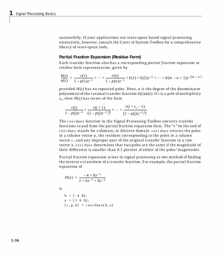
1 Signal Processing Basics
1-36
successfully. If your applications use state-space based signal processingextensively, however, consult the Contr ol System Toolbox for a comprehensivelibrary of state-space tools.
Partial Fraction Expansion (Residue Form)Each transfer function also has a corresponding partial fraction expansion orresidue form representation, given by
provided H(z) has no repeated poles. Here, n is the degree of the denominatorpolynomial of the rational transfer function b(z)/a(z). If r is a pole of multiplicitysr, then H(z) has terms of the form
The residuez function in the Signal Processing Toolbox converts transferfunctions to and from the partial fraction expansion form. The “z” on the end ofresiduez stands for z-domain, or discrete domain. residuez returns the polesin a column vector p, the residues corresponding to the poles in a columnvector r, and any improper part of the original transfer function in a rowvector k. residuez determines that two poles are the same if the magnitude oftheir difference is smaller than 0.1 percent of either of the poles’ magnitudes.
Partial fraction expansion arises in signal processing as one method of findingthe inverse z-transform of a transfer function. For example, the partial fractionexpansion of
is
b = [-4 8];a = [1 6 8];[r,p,k] = residuez(b,a)
b z( )a z( )----------
r 1( )1 p 1( )z 1––----------------------------
r n( )1 p n( )z 1––----------------------------- k 1( ) k 2( )z 1– k m n 1+–( )z m n–( )–+ + + + + +=
r j( )1 p j( )z 1––---------------------------
r j 1+( )
1 p j( )z 1––( )2-----------------------------------
r j sr 1–+( )
1 p j( )z 1––( )sr------------------------------------+ + +
H z( )4– 8z 1–+
1 6z 1– 8z 2–+ +----------------------------------------=
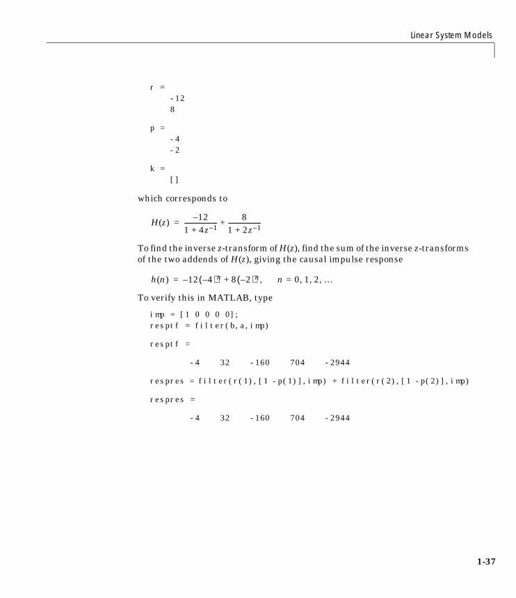
Linear System Models
1-37
r =-128
p =-4-2
k =[]
which corresponds to
To find the inverse z-transform of H(z), find the sum of the inverse z-transformsof the two addends of H(z), giving the causal impulse response
To verify this in MATLAB, type
imp = [1 0 0 0 0];resptf = filter(b,a,imp)
resptf =
-4 32 -160 704 -2944
respres = filter(r(1),[1 -p(1)],imp) + filter(r(2),[1 -p(2)],imp)
respres =
-4 32 -160 704 -2944
H z( )12–
1 4z 1–+---------------------
81 2z 1–+---------------------+=
h n( ) 12– 4–( )n 8 2–( )n+ n 0 1 2 …, , ,=,=
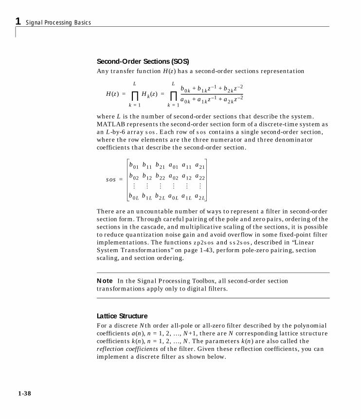
1 Signal Processing Basics
1-38
Second-Order Sections (SOS)Any transfer function H(z) has a second-order sections representation
where L is the number of second-order sections that describe the system.MATLAB represents the second-order section form of a discrete-time system asan L-by-6 array sos. Each row of sos contains a single second-order section,where the row elements are the three numerator and three denominatorcoefficients that describe the second-order section.
There are an uncountable number of ways to represent a filter in second-ordersection form. Through careful pairing of the pole and zero pairs, ordering of thesections in the cascade, and multiplicative scaling of the sections, it is possibleto reduce quantization noise gain and avoid overflow in some fixed-point filterimplementations. The functions zp2sos and ss2sos, described in “LinearSystem Transformations” on page 1-43, perform pole-zero pairing, sectionscaling, and section ordering.
Note In the Signal Processing Toolbox, all second-order sectiontransformations apply only to digital filters.
Lattice StructureFor a discrete Nth order all-pole or all-zero filter described by the polynomialcoefficients a(n), n = 1, 2, …, N+1, there are N corresponding lattice structurecoefficients k(n), n = 1, 2, …, N. The parameters k(n) are also called thereflection coefficients of the filter. Given these reflection coefficients, you canimplement a discrete filter as shown below.
H z( ) Hk z( )
k 1=
L
∏b0k b1kz 1– b2kz 2–+ +
a0k a1kz 1– a2kz 2–+ +----------------------------------------------------------
k 1=
L
∏= =
sos
b01 b11 b21 a01 a11 a21
b02 b12 b22 a02 a12 a22
b0L b1L b2L a0L a1L a2L
=
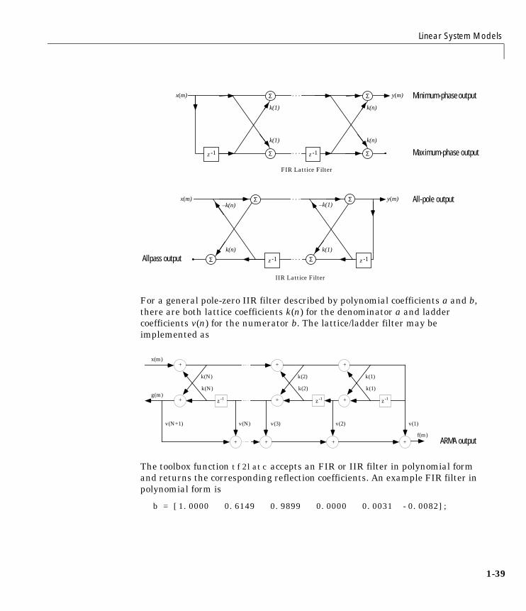
Linear System Models
1-39
For a general pole-zero IIR filter described by polynomial coefficients a and b,there are both lattice coefficients k(n) for the denominator a and laddercoefficients v(n) for the numerator b. The lattice/ladder filter may beimplemented as
The toolbox function tf2latc accepts an FIR or IIR filter in polynomial formand returns the corresponding reflection coefficients. An example FIR filter inpolynomial form is
b = [1.0000 0.6149 0.9899 0.0000 0.0031 -0.0082];
Σ
Σ
z -1
y(m)
k(1)
k(1)
Σ
Σ
k(n)
k(n)
. . .
. . . z -1
FIR Lattice Filter
x(m)
x(m)
Σ
Σ y(m)
k(1)
–k(1)Σ
k(n)
–k(n). . .
. . .z -1 Σ z -1
IIR Lattice Filter
Minimum-phase output
All-pole output
Maximum-phase output
Allpass output
z-1+
+x(m)
g(m)
+
k(N)
k(N)
z-1+
+
k(2)
k(2)
z-1+
+
k(1)
k(1)
++ +
v(N+1) v(N) v(3) v(2) v(1)
f(m)ARMA output
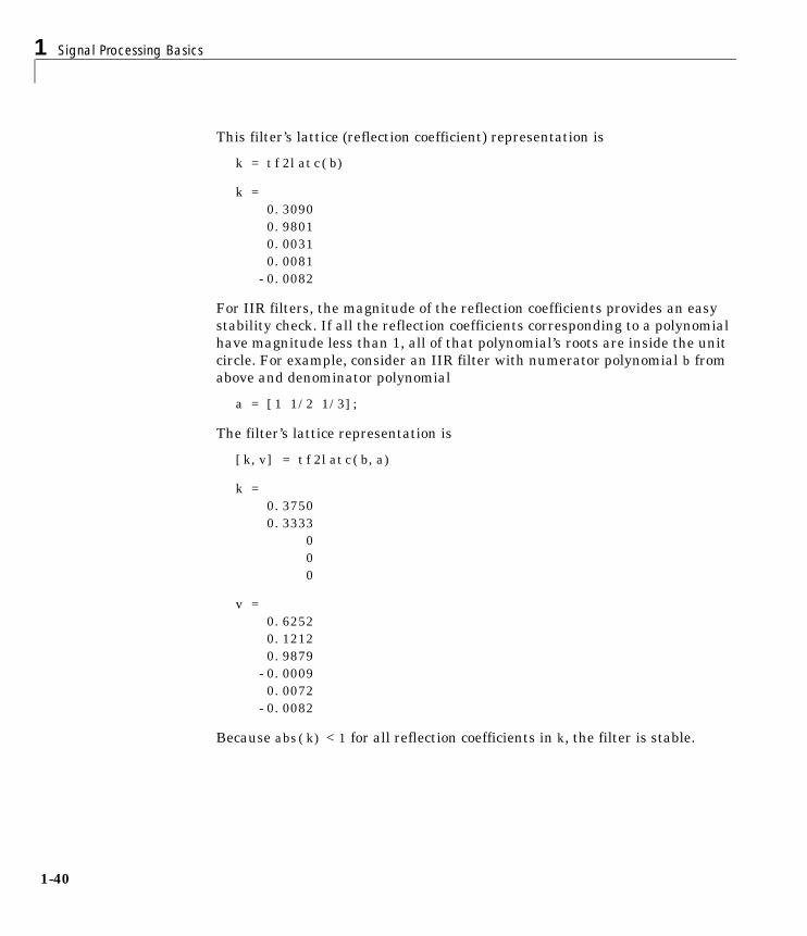
1 Signal Processing Basics
1-40
This filter’s lattice (reflection coefficient) representation is
k = tf2latc(b)
k = 0.3090
0.98010.00310.0081-0.0082
For IIR filters, the magnitude of the reflection coefficients provides an easystability check. If all the reflection coefficients corresponding to a polynomialhave magnitude less than 1, all of that polynomial’s roots are inside the unitcircle. For example, consider an IIR filter with numerator polynomial b fromabove and denominator polynomial
a = [1 1/2 1/3];
The filter’s lattice representation is
[k,v] = tf2latc(b,a)
k = 0.3750 0.3333 0 0 0
v = 0.6252 0.1212 0.9879 -0.0009 0.0072 -0.0082
Because abs(k) < 1 for all reflection coefficients in k, the filter is stable.

Linear System Models
1-41
The function latc2tf calculates the polynomial coefficients for a filter from itslattice (reflection) coefficients. Given the reflection coefficient vector k(above),the corresponding polynomial form is
b = latc2tf(k)
b = 1.0000 0.6149 0.9899 -0.0000 0.0031 -0.0082
The lattice or lattice/ladder coefficients can be used to implement the filterusing the function latcfilt.
Convolution MatrixIn signal processing, convolving two vectors or matrices is equivalent tofiltering one of the input operands by the other. This relationship permits therepresentation of a digital filter as a convolution matrix.
Given any vector, the toolbox function convmtx generates a matrix whose innerproduct with another vector is equivalent to the convolution of the two vectors.The generated matrix represents a digital filter that you can apply to anyvector of appropriate length; the inner dimension of the operands must agreeto compute the inner product.
The convolution matrix for a vector b, representing the numerator coefficientsfor a digital filter, is
b = [1 2 3]; x = randn(3,1);C = convmtx(b',3)
C =1 0 02 1 03 2 10 3 20 0 3
Two equivalent ways to convolve b with x are as follows.
y1 = C*x;y2 = conv(b,x);

1 Signal Processing Basics
1-42
Continuous-Time System ModelsThe continuous-time system models are representational schemes for analogfilters. Many of the discrete-time system models described earlier are alsoappropriate for the representation of continuous-time systems:
• State-space form
• Partial fraction expansion
• Transfer function
• Zero-pole-gain form
It is possible to represent any system of linear time-invariant differentialequations as a set of first-order differential equations. In matrix or state-spaceform, you can express the equations as
where u is a vector of nu inputs, x is an nx-element state vector, and y is a vectorof ny outputs. In MATLAB, store A, B, C, and D in separate rectangular arrays.
An equivalent representation of the state-space system is the Laplacetransform transfer function description
where
For single-input, single-output systems, this form is given by
Given the coefficients of a Laplace transform transfer function, residuedetermines the partial fraction expansion of the system. See the description ofresidue in the MATLAB documentation for details.
The factored zero-pole-gain form is
x· Ax Bu+=
y Cx Du+=
Y s( ) H s( )U s( )=
H s( ) C sI A–( ) 1– B D+=
H s( )b s( )a s( )----------
b 1( )snb b 2( )snb 1– b nb 1+( )+ + +a 1( )sna a 2( )sna 1– a na 1+( )+ + +-------------------------------------------------------------------------------------------------= =
H s( )z s( )p s( )---------- k s z 1( )–( ) s z 2( )–( ) s z n( )–( )
s p 1( )–( ) s p 2( )–( ) s p n( )–( )--------------------------------------------------------------------------------= =

Linear System Models
1-43
As in the discrete-time case, MATLAB stores polynomial coefficients in rowvectors in descending powers of s. MATLAB stores polynomial roots, or zerosand poles, in column vectors.
Linear System TransformationsThe Signal Processing Toolbox provides a number of functions that convertbetween the various linear system models; see Chapter 7, “FunctionReference,” for a complete description of each. You can use the following chartto find an appropriate transfer function: find the row of the model to convertfrom on the left side of the chart and the column of the model to convert to onthe top of the chart and read the function name(s) at the intersection of the rowand column.
Many of the toolbox filter design functions use these functions internally. Forexample, the zp2ss function converts the poles and zeros of an analogprototype into the state-space form required for creation of a Butterworth,Chebyshev, or elliptic filter. Once in state-space form, the filter design functionperforms any required frequency transformation, that is, it transforms theinitial lowpass design into a bandpass, highpass, or bandstop filter, or alowpass filter with the desired cutoff frequency. See the descriptions of the
Transfer function
State- space
Zero-pole-gain
Partial fraction
Lattice filter
Second-order sections
Convolutionmatrix
Transfer function
tf2ss tf2zproots
residuezresidue
tf2latc convmtx
State-space ss2tf ss2zp ss2sos
Zero-pole- gain
zp2tf poly
zp2ss zp2sos
Partial fraction
residuezresidue
Lattice filter latc2tf
SOS sos2tf sos2ss sos2zp
Convolutionmatrix

1 Signal Processing Basics
1-44
individual filter design functions in Chapter 7, “Function Reference,” for moredetails.
Note In the Signal Processing Toolbox, all second-order sectiontransformations apply only to digital filters.

Discrete Fourier Transform
1-45
Discrete Fourier TransformThe discrete Fourier transform, or DFT, is the primary tool of digital signalprocessing. The foundation of the Signal Processing Toolbox is the fast Fouriertransform (FFT), a method for computing the DFT with reduced executiontime. Many of the toolbox functions (including z-domain frequency response,spectrum and cepstrum analysis, and some filter design and implementationfunctions) incorporate the FFT.
MATLAB provides the functions fft and ifft to compute the discrete Fouriertransform and its inverse, respectively. For the input sequence x and itstransformed version X (the discrete-time Fourier transform at equally spacedfrequencies around the unit circle), the two functions implement therelationships
In these equations, the series subscripts begin with 1 instead of 0 because ofMATLAB’s vector indexing scheme, and
Note MATLAB uses a negative j for the fft function. This is an engineeringconvention; physics and pure mathematics typically use a positive j.
fft, with a single input argument x, computes the DFT of the input vector ormatrix. If x is a vector, fft computes the DFT of the vector; if x is a rectangulararray, fft computes the DFT of each array column.
X k 1+( ) x n 1+( )Wnkn
n 0=
N 1–
=
x n 1+( )1N---- X k 1+( )Wn
kn–
k 0=
N 1–
=
WN ej–
2πN-------
=
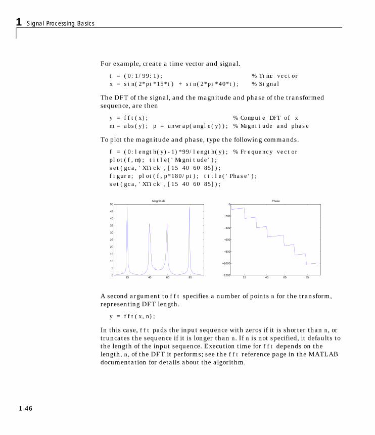
1 Signal Processing Basics
1-46
For example, create a time vector and signal.
t = (0:1/99:1); % Time vectorx = sin(2*pi*15*t) + sin(2*pi*40*t); % Signal
The DFT of the signal, and the magnitude and phase of the transformedsequence, are then
y = fft(x); % Compute DFT of xm = abs(y); p = unwrap(angle(y)); % Magnitude and phase
To plot the magnitude and phase, type the following commands.
f = (0:length(y)-1)*99/length(y); % Frequency vectorplot(f,m); title('Magnitude');set(gca,'XTick',[15 40 60 85]);figure; plot(f,p*180/pi); title('Phase');set(gca,'XTick',[15 40 60 85]);
A second argument to fft specifies a number of points n for the transform,representing DFT length.
y = fft(x,n);
In this case, fft pads the input sequence with zeros if it is shorter than n, ortruncates the sequence if it is longer than n. If n is not specified, it defaults tothe length of the input sequence. Execution time for fft depends on thelength, n, of the DFT it performs; see the fft reference page in the MATLABdocumentation for details about the algorithm.
15 40 60 850
5
10
15
20
25
30
35
40
45
50Magnitude
15 40 60 85−1200
−1000
−800
−600
−400
−200
0Phase
Discrete Fourier Transform
1-47
The inverse discrete Fourier transform function ifft also accepts an inputsequence and, optionally, the number of desired points for the transform. Trythe example below; the original sequence x and the reconstructed sequence areidentical (within rounding error).
t = (0:1/255:1);x = sin(2*pi*120*t);y = real(ifft(fft(x)));
This toolbox also includes functions for the two-dimensional FFT and itsinverse, fft2 and ifft2. These functions are useful for two-dimensional signalor image processing; see the descriptions in Chapter 7, “Function Reference,”for details.
It is sometimes convenient to rearrange the output of the fft or fft2 functionso the zero frequency component is at the center of the sequence. The MATLABfunction fftshiftmoves the zero frequency component to the center of a vectoror matrix.

1 Signal Processing Basics
1-48
Selected BibliographyAlgorithm development for the Signal Processing Toolbox has drawn heavilyupon the references listed below. All are recommended to the interested readerwho needs to know more about signal processing than is covered in thismanual.
[1] Crochiere, R.E., and L.R. Rabiner. Multi-Rate Signal Processing.Englewood Cliffs, NJ: Prentice Hall, 1983. Pgs. 88-91.
[2] IEEE. Programs for Digital Signal Processing. IEEE Press. New York: JohnWiley & Sons, 1979.
[3] Jackson, L.B. Digital Filters and Signal Processing. Third Ed. Boston:Kluwer Academic Publishers, 1989.
[4] Kay, S.M. Modern Spectral Estimation. Englewood Cliffs, NJ: Prentice Hall,1988.
[5] Oppenheim, A.V., and R.W. Schafer. Discrete-Time Signal Processing.Englewood Cliffs, NJ: Prentice Hall, 1989.
[6] Parks, T.W., and C.S. Burrus. Digital Filter Design. New York: John Wiley& Sons, 1987.
[7] Pratt,W.K. Digital Image Processing. New York: John Wiley & Sons, 1991.
[8] Percival, D.B., and A.T. Walden. Spectral Analysis for PhysicalApplications: Multitaper and Conventional Univariate Techniques. Cambridge:Cambridge University Press, 1993.
[9] Proakis, J.G., and D.G. Manolakis. Digital Signal Processing: Principles,Algorithms, and Applications. Upper Saddle River, NJ: Prentice Hall, 1996.
[10] Rabiner, L.R., and B. Gold. Theory and Application of Digital SignalProcessing. Englewood Cliffs, NJ: Prentice Hall, 1975.
[11] Welch, P.D. “The Use of Fast Fourier Transform for the Estimation ofPower Spectra: A Method Based on Time Averaging Over Short, ModifiedPeriodograms.” IEEE Trans. Audio Electroacoust. Vol. AU-15 (June 1967).Pgs. 70-73.

2
Filter Design
Filter Requirements and Specification . . . . . . . . 2-2
IIR Filter Design . . . . . . . . . . . . . . . . . . 2-4Classical IIR Filter Design Using Analog Prototyping . . . . 2-6Comparison of Classical IIR Filter Types . . . . . . . . . 2-8
FIR Filter Design . . . . . . . . . . . . . . . . . . 2-16Linear Phase Filters . . . . . . . . . . . . . . . . . 2-17Windowing Method . . . . . . . . . . . . . . . . . . 2-18Multiband FIR Filter Design with Transition Bands . . . . 2-22Constrained Least Squares FIR Filter Design . . . . . . . 2-27Arbitrary-Response Filter Design . . . . . . . . . . . . 2-31
Special Topics in IIR Filter Design . . . . . . . . . . 2-37Analog Prototype Design . . . . . . . . . . . . . . . 2-38Frequency Transformation . . . . . . . . . . . . . . . 2-38Filter Discretization . . . . . . . . . . . . . . . . . 2-41
Selected Bibliography . . . . . . . . . . . . . . . 2-45

2 Filter Design
2-2
OverviewThe Signal Processing Toolbox provides functions that support a range of filterdesign methodologies. The following sections explain how to apply the filterdesign tools to Infinite Impulse Response (IIR) and Finite Impulse Response(FIR) filter design problems:
• “Filter Requirements and Specification”
• “IIR Filter Design”
• “FIR Filter Design”
• “Special Topics in IIR Filter Design”
• “Selected Bibliography”
Filter Requirements and Specification
2-3
Filter Requirements and SpecificationThe goal of filter design is to perform frequency dependent alteration of a datasequence. A possible requirement might be to remove noise above 30 Hz froma data sequence sampled at 100 Hz. A more rigorous specification might call fora specific amount of passband ripple, stopband attenuation, or transitionwidth. A very precise specification could ask to achieve the performance goalswith the minimum filter order, or it could call for an arbitrary magnitudeshape, or it might require an FIR filter.
Filter design methods differ primarily in how performance is specified. For“loosely specified” requirements, as in the first case above, a Butterworth IIRfilter is often sufficient. To design a fifth-order 30 Hz lowpass Butterworthfilter and apply it to the data in vector x,
[b,a] = butter(5,30/50);y = filter(b,a,x);
The second input argument to butter specifies the cutoff frequency,normalized to half the sampling frequency (the Nyquist frequency).
Frequency Normalization in the Signal Processing Toolbox All of thefilter design functions operate with normalized frequencies, so they do notrequire the system sampling rate as an extra input argument. This toolboxuses the convention that unit frequency is the Nyquist frequency, defined ashalf the sampling frequency. The normalized frequency, therefore, is always inthe interval 0 ≤ f ≤ 1. For a system with a 1000 Hz sampling frequency, 300 Hzis 300/500 = 0.6. To convert normalized frequency to angular frequencyaround the unit circle, multiply by π. To convert normalized frequency back tohertz, multiply by half the sample frequency.
More rigorous filter requirements traditionally include passband ripple (Rp, indecibels), stopband attenuation (Rs, in decibels), and transition width (Ws-Wp,in hertz).
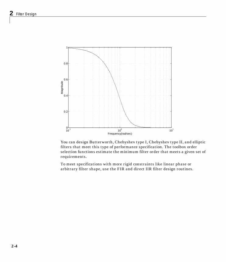
2 Filter Design
2-4
You can design Butterworth, Chebyshev type I, Chebyshev type II, and ellipticfilters that meet this type of performance specification. The toolbox orderselection functions estimate the minimum filter order that meets a given set ofrequirements.
To meet specifications with more rigid constraints like linear phase orarbitrary filter shape, use the FIR and direct IIR filter design routines.
10-1
100
101
0
0.2
0.4
0.6
0.8
1
Frequency(rad/sec)
Mag
nitu
de
IIR Filter Design
2-5
IIR Filter DesignThe primary advantage of IIR filters over FIR filters is that they typically meeta given set of specifications with a much lower filter order than a correspondingFIR filter. Although IIR filters have nonlinear phase, data processing withinMATLAB is commonly performed “off-line,” that is, the entire data sequence isavailable prior to filtering. This allows for a noncausal, zero-phase filteringapproach (via the filtfilt function), which eliminates the nonlinear phasedistortion of an IIR filter.
The classical IIR filters, Butterworth, Chebyshev types I and II, elliptic, andBessel, all approximate the ideal “brick wall” filter in different ways. Thistoolbox provides functions to create all these types of classical IIR filters in boththe analog and digital domains (except Bessel, for which only the analog caseis supported), and in lowpass, highpass, bandpass, and bandstopconfigurations. For most filter types, you can also find the lowest filter orderthat fits a given filter specification in terms of passband and stopbandattenuation, and transition width(s).
The direct filter design function yulewalk finds a filter with magnituderesponse approximating a desired function. This is one way to create amultiband bandpass filter.
You can also use the parametric modeling or system identification functions todesign IIR filters. These functions are discussed in “Parametric Modeling” onpage 4-11.
The generalized Butterworth design function maxflat is discussed in thesection “Generalized Butterworth Filter Design” on page 2-14.
The following table summarizes the various filter methods in the toolbox andlists the functions available to implement these methods.

2 Filter Design
2-6
Method Description Functions
AnalogPrototyping
Using the poles and zeros ofa classical lowpassprototype filter in thecontinuous (Laplace)domain, obtain a digitalfilter through frequencytransformation and filterdiscretization.
Complete design functions:
besself, butter, cheby1, cheby2, ellip
Order estimation functions:
buttord, cheb1ord, cheb2ord, ellipord
Lowpass analog prototype functions:
besselap, buttap, cheb1ap, cheb2ap,ellipap
Frequency transformation functions:
lp2bp, lp2bs, lp2hp, lp2lp
Filter discretization functions:
bilinear, impinvar
Direct Design Design digital filter directlyin the discrete time-domainby approximating apiecewise linear magnituderesponse.
yulewalk
GeneralizedButterworthDesign
Design lowpassButterworth filters withmore zeros than poles.
maxflat
ParametricModeling
Find a digital filter thatapproximates a prescribedtime or frequency domainresponse. (See the SystemIdentification Toolbox for anextensive collection ofparametric modeling tools.)
Time-domain modeling functions:
lpc, prony, stmcb
Frequency-domain modeling functions:
invfreqs, invfreqz
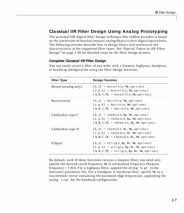
IIR Filter Design
2-7
Classical IIR Filter Design Using Analog PrototypingThe principal IIR digital filter design technique this toolbox provides is basedon the conversion of classical lowpass analog filters to their digital equivalents.The following sections describe how to design filters and summarize thecharacteristics of the supported filter types. See “Special Topics in IIR FilterDesign” on page 2-38 for detailed steps on the filter design process.
Complete Classical IIR Filter DesignYou can easily create a filter of any order with a lowpass, highpass, bandpass,or bandstop configuration using the filter design functions.
By default, each of these functions returns a lowpass filter; you need onlyspecify the desired cutoff frequency Wn in normalized frequency (Nyquistfrequency = 1 Hz). For a highpass filter, append the string 'high' to thefunction’s parameter list. For a bandpass or bandstop filter, specify Wn as atwo-element vector containing the passband edge frequencies, appending thestring 'stop' for the bandstop configuration.
Filter Type Design Function
Bessel (analog only) [b,a] = besself(n,Wn,options)[z,p,k] = besself(n,Wn,options)[A,B,C,D] = besself(n,Wn,options)
Butterworth [b,a] = butter(n,Wn,options)[z,p,k] = butter(n,Wn,options)[A,B,C,D] = butter(n,Wn,options)
Chebyshev type I [b,a] = cheby1(n,Rp,Wn,options)[z,p,k] = cheby1(n,Rp,Wn,options)[A,B,C,D] = cheby1(n,Rp,Wn,options)
Chebyshev type II [b,a] = cheby2(n,Rs,Wn,options)[z,p,k] = cheby2(n,Rs,Wn,options)[A,B,C,D] = cheby2(n,Rs,Wn,options)
Elliptic [b,a] = ellip(n,Rp,Rs,Wn,options)[z,p,k] = ellip(n,Rp,Rs,Wn,options)[A,B,C,D] = ellip(n,Rp,Rs,Wn,options)

2 Filter Design
2-8
Here are some example digital filters.
[b,a] = butter(5,0.4); % Lowpass Butterworth[b,a] = cheby1(4,1,[0.4 0.7]); % Bandpass Chebyshev type I[b,a] = cheby2(6,60,0.8,'high'); % Highpass Chebyshev type II[b,a] = ellip(3,1,60,[0.4 0.7],'stop'); % Bandstop elliptic
To design an analog filter, perhaps for simulation, use a trailing 's' andspecify cutoff frequencies in rad/s.
[b,a] = butter(5,.4,'s'); % Analog Butterworth filter
All filter design functions return a filter in the transfer function,zero-pole-gain, or state-space linear system model representation, dependingon how many output arguments are present.
Note All classical IIR lowpass filters are ill-conditioned for extremely lowcut-off frequencies. Therefore, instead of designing a lowpass IIR filter with avery narrow passband, it can be better to design a wider passband anddecimate the input signal.
Designing IIR Filters to Frequency Domain SpecificationsThis toolbox provides order selection functions that calculate the minimumfilter order that meets a given set of requirements.
These are useful in conjunction with the filter design functions. Suppose youwant a bandpass filter with a passband from 1000 to 2000 Hz, stopbandsstarting 500 Hz away on either side, a 10 kHz sampling frequency, at most 1 dB
Filter Type Order Estimation Function
Butterworth [n,Wn] = buttord(Wp,Ws,Rp,Rs)
Chebyshev type I [n,Wn] = cheb1ord(Wp, Ws, Rp, Rs)
Chebyshev type II [n,Wn] = cheb2ord(Wp, Ws, Rp, Rs)
Elliptic [n,Wn] = ellipord(Wp, Ws, Rp, Rs)
IIR Filter Design
2-9
of passband ripple, and at least 60 dB of stopband attenuation. You can meetthese specifications by using the butter function as follows.
[n,Wn] = buttord([1000 2000]/5000,[500 2500]/5000,1,60)
n = 12Wn = 0.1951 0.4080
[b,a] = butter(n,Wn);
An elliptic filter that meets the same requirements is given by
[n,Wn] = ellipord([1000 2000]/5000,[500 2500]/5000,1,60)
n = 5Wn = 0.2000 0.4000
[b,a] = ellip(n,1,60,Wn);
These functions also work with the other standard band configurations, as wellas for analog filters; see Chapter 7, “Function Reference,” for details.
Comparison of Classical IIR Filter TypesThe toolbox provides five different types of classical IIR filters, each optimal insome way. This section shows the basic analog prototype form for each andsummarizes major characteristics.
Butterworth FilterThe Butterworth filter provides the best Taylor Series approximation to theideal lowpass filter response at analog frequencies and ; for anyorder N, the magnitude squared response has 2N-1 zero derivatives at theselocations (maximally flat at and ). Response is monotonic overall,decreasing smoothly from to . at .
Ω 0= Ω ∞=
Ω 0= Ω ∞=Ω 0= Ω ∞= H jΩ( ) 1 2⁄= Ω 1=

2 Filter Design
2-10
Chebyshev Type I FilterThe Chebyshev type I filter minimizes the absolute difference between theideal and actual frequency response over the entire passband by incorporatingan equal ripple of Rp dB in the passband. Stopband response is maximally flat.The transition from passband to stopband is more rapid than for theButterworth filter. at .
10-1
100
101
0
0.2
0.4
0.6
0.8
1
Frequency(rad/sec)
Mag
nitu
de
H jΩ( ) 10 Rp 20⁄–= Ω 1=
10-1
100
101
0
0.2
0.4
0.6
0.8
1
Frequency(rad/sec)
Mag
nitu
de

IIR Filter Design
2-11
Chebyshev Type II FilterThe Chebyshev type II filter minimizes the absolute difference between theideal and actual frequency response over the entire stopband by incorporatingan equal ripple of Rs dB in the stopband. Passband response is maximally flat.
The stopband does not approach zero as quickly as the type I filter (and doesnot approach zero at all for even-valued filter order n). The absence of ripple inthe passband, however, is often an important advantage.at .
Elliptic FilterElliptic filters are equiripple in both the passband and stopband. Theygenerally meet filter requirements with the lowest order of any supported filtertype. Given a filter order n, passband ripple Rp in decibels, and stopband rippleRs in decibels, elliptic filters minimize transition width. at
.
H jΩ( ) 10 Rs 20⁄–=
Ω 1=
10-1
100
101
0
0.2
0.4
0.6
0.8
1
Frequency(rad/sec)
Mag
nitu
de
H jΩ( ) 10 Rp 20⁄–=
Ω 1=

2 Filter Design
2-12
Bessel FilterAnalog Bessel lowpass filters have maximally flat group delay at zerofrequency and retain nearly constant group delay across the entire passband.Filtered signals therefore maintain their waveshapes in the passbandfrequency range. Frequency mapped and digital Bessel filters, however, do nothave this maximally flat property; this toolbox supports only the analog casefor the complete Bessel filter design function.
Bessel filters generally require a higher filter order than other filters forsatisfactory stopband attenuation. at and decreases asfilter order n increases.
10-1
100
101
0
0.2
0.4
0.6
0.8
1
Frequency(rad/sec)
Mag
nitu
de
H jΩ( ) 1 2⁄< Ω 1=
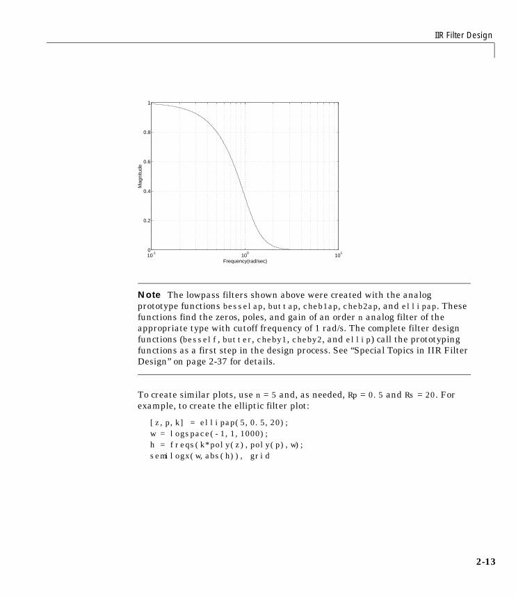
IIR Filter Design
2-13
Note The lowpass filters shown above were created with the analogprototype functions besselap, buttap, cheb1ap, cheb2ap, and ellipap. Thesefunctions find the zeros, poles, and gain of an order n analog filter of theappropriate type with cutoff frequency of 1 rad/s. The complete filter designfunctions (besself, butter, cheby1, cheby2, and ellip) call the prototypingfunctions as a first step in the design process. See “Special Topics in IIR FilterDesign” on page 2-37 for details.
To create similar plots, use n = 5 and, as needed, Rp = 0.5 and Rs = 20. Forexample, to create the elliptic filter plot:
[z,p,k] = ellipap(5,0.5,20);w = logspace(-1,1,1000);h = freqs(k*poly(z),poly(p),w);semilogx(w,abs(h)), grid
10-1
100
101
0
0.2
0.4
0.6
0.8
1
Frequency(rad/sec)
Mag
nitu
de

2 Filter Design
2-14
Direct IIR Filter DesignThis toolbox uses the term direct methods to describe techniques for IIR designthat find a filter based on specifications in the discrete domain. Unlike theanalog prototyping method, direct design methods are not constrained to thestandard lowpass, highpass, bandpass, or bandstop configurations. Rather,these functions design filters with an arbitrary, perhaps multiband, frequencyresponse. This section discusses the yulewalk function, which is intendedspecifically for filter design; “Parametric Modeling” on page 4-11 discussesother methods that may also be considered direct, such as Prony’s method,Linear Prediction, the Steiglitz-McBride method, and inverse frequencydesign.
The yulewalk function designs recursive IIR digital filters by fitting a specifiedfrequency response. yulewalk’s name reflects its method for finding the filter’sdenominator coefficients: it finds the inverse FFT of the ideal desired powerspectrum and solves the “modified Yule-Walker equations” using the resultingautocorrelation function samples. The statement
[b,a] = yulewalk(n,f,m)
returns row vectors b and a containing the n+1 numerator and denominatorcoefficients of the order n IIR filter whose frequency-magnitude characteristicsapproximate those given in vectors f and m. f is a vector of frequency pointsranging from 0 to 1, where 1 represents the Nyquist frequency. m is a vectorcontaining the desired magnitude response at the points in f. f and m candescribe any piecewise linear shape magnitude response, including amultiband response. The FIR counterpart of this function is fir2, which alsodesigns a filter based on an arbitrary piecewise linear magnitude response. See“FIR Filter Design” on page 2-16 for details.
Note that yulewalk does not accept phase information, and no statements aremade about the optimality of the resulting filter.
Design a multiband filter with yulewalk, and plot the desired and actualfrequency response.
m = [0 0 1 1 0 0 1 1 0 0];f = [0 0.1 0.2 0.3 0.4 0.5 0.6 0.7 0.8 1];[b,a] = yulewalk(10,f,m);[h,w] = freqz(b,a,128);plot(f,m,w/pi,abs(h))

IIR Filter Design
2-15
Generalized Butterworth Filter DesignThe toolbox function maxflat enables you to design generalized Butterworthfilters, that is, Butterworth filters with differing numbers of zeros and poles.This is desirable in some implementations where poles are more expensivecomputationally than zeros. maxflat is just like the butter function, exceptthat it you can specify two orders (one for the numerator and one for thedenominator) instead of just one. These filters are maximally flat. This meansthat the resulting filter is optimal for any numerator and denominator orders,with the maximum number of derivatives at 0 and the Nyquist frequency ω = πboth set to 0.
For example, when the two orders are the same, maxflat is the same as butter.
[b,a] = maxflat(3,3,0.25)
b = 0.0317 0.0951 0.0951 0.0317
a = 1.0000 -1.4590 0.9104 -0.1978
0 0.1 0.2 0.3 0.4 0.5 0.6 0.7 0.8 0.9 10
0.2
0.4
0.6
0.8
1
1.2

2 Filter Design
2-16
[b,a] = butter(3,0.25)
b = 0.0317 0.0951 0.0951 0.0317
a = 1.0000 -1.4590 0.9104 -0.1978
However, maxflat is more versatile because it allows you to design a filter withmore zeros than poles.
[b,a] = maxflat(3,1,0.25)
b = 0.0950 0.2849 0.2849 0.0950
a = 1.0000 -0.2402
The third input to maxflat is the half-power frequency, a frequency between0 and 1 with a desired magnitude response of .
You can also design linear phase filters that have the maximally flat propertyusing the 'sym' option.
maxflat(4,'sym',0.3)
ans = 0.0331 0.2500 0.4337 0.2500 0.0331
For complete details of the maxflat algorithm, see Selesnick and Burrus [2].
1 2⁄
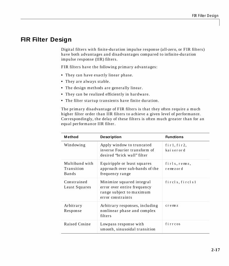
FIR Filter Design
2-17
FIR Filter DesignDigital filters with finite-duration impulse response (all-zero, or FIR filters)have both advantages and disadvantages compared to infinite-durationimpulse response (IIR) filters.
FIR filters have the following primary advantages:
• They can have exactly linear phase.
• They are always stable.
• The design methods are generally linear.
• They can be realized efficiently in hardware.
• The filter startup transients have finite duration.
The primary disadvantage of FIR filters is that they often require a muchhigher filter order than IIR filters to achieve a given level of performance.Correspondingly, the delay of these filters is often much greater than for anequal performance IIR filter.
Method Description Functions
Windowing Apply window to truncatedinverse Fourier transform ofdesired “brick wall” filter
fir1, fir2,kaiserord
Multiband withTransitionBands
Equiripple or least squaresapproach over sub-bands of thefrequency range
firls, remez,remezord
ConstrainedLeast Squares
Minimize squared integralerror over entire frequencyrange subject to maximumerror constraints
fircls, fircls1
ArbitraryResponse
Arbitrary responses, includingnonlinear phase and complexfilters
cremez
Raised Cosine Lowpass response withsmooth, sinusoidal transition
firrcos

2 Filter Design
2-18
Linear Phase FiltersExcept for cremez, all of the FIR filter design functions design linear phasefilters only. The filter coefficients, or “taps,” of such filters obey either an evenor odd symmetry relation. Depending on this symmetry, and on whether theorder n of the filter is even or odd, a linear phase filter (stored in length n+1vector b) has certain inherent restrictions on its frequency response.
The phase delay and group delay of linear phase FIR filters are equal andconstant over the frequency band. For an order n linear phase FIR filter, thegroup delay is n/2, and the filtered signal is simply delayed by n/2 time steps(and the magnitude of its Fourier transform is scaled by the filter’s magnituderesponse). This property preserves the wave shape of signals in the passband;that is, there is no phase distortion.
The functions fir1, fir2, firls, remez, fircls, fircls1, and firrcos alldesign type I and II linear phase FIR filters by default. Both firls and remezdesign type III and IV linear phase FIR filters given a 'hilbert' or'differentiator' flag. cremez can design any type of linear phase filter, andnonlinear phase filters as well.
Note Because the frequency response of a type II filter is zero at the Nyquistfrequency (“high” frequency), fir1 does not design type II highpass andbandstop filters. For odd-valued n in these cases, fir1 adds 1 to the order andreturns a type I filter.
Linear Phase Filter Type
Filter Order Symmetry of Coefficients
Response H(f), f = 0
Response H(f), f = 1 (Nyquist)
Type I Even even: No restriction No restriction
Type II Odd No restriction H(1) = 0
Type III Even odd: H(0) = 0 H(1) = 0
Type IV Odd H(0) = 0 No restriction
b k( ) b n 2 k–+( ) k 1= … n 1+, , ,=
b k( ) b– n 2 k–+( ) k 1= … n 1+, , ,=

FIR Filter Design
2-19
Windowing MethodConsider the ideal, or “brick wall,” digital lowpass filter with a cutoff frequencyof ω0 rad/s. This filter has magnitude 1 at all frequencies with magnitude lessthan ω0, and magnitude 0 at frequencies with magnitude between ω0 and π. Itsimpulse response sequence h(n) is
This filter is not implementable since its impulse response is infinite andnoncausal. To create a finite-duration impulse response, truncate it byapplying a window. By retaining the central section of impulse response in thistruncation, you obtain a linear phase FIR filter. For example, a length 51 filterwith a lowpass cutoff frequency ω0 of rad/s is
b = 0.4*sinc(0.4*(-25:25));
The window applied here is a simple rectangular or “boxcar” window. ByParseval’s theorem, this is the length 51 filter that best approximates the ideallowpass filter, in the integrated least squares sense. The following commandsdisplay the filter’s frequency response.
[H,w] = freqz(b,1,512,2);s.xunits = 'rad/sample';s.yunits = 'squared';s.plot = 'mag'; % Plot magnitude only.freqzplot(H,w,s)title('Truncated Sinc Lowpass FIR Filter');
h n( )1
2π------ H ω( )ejωn ωd
π–
π
1
2π------ ejωn ωd
ω0–
ω0
ω0π
-------sincω0π
-------n( )= = =
0.4π
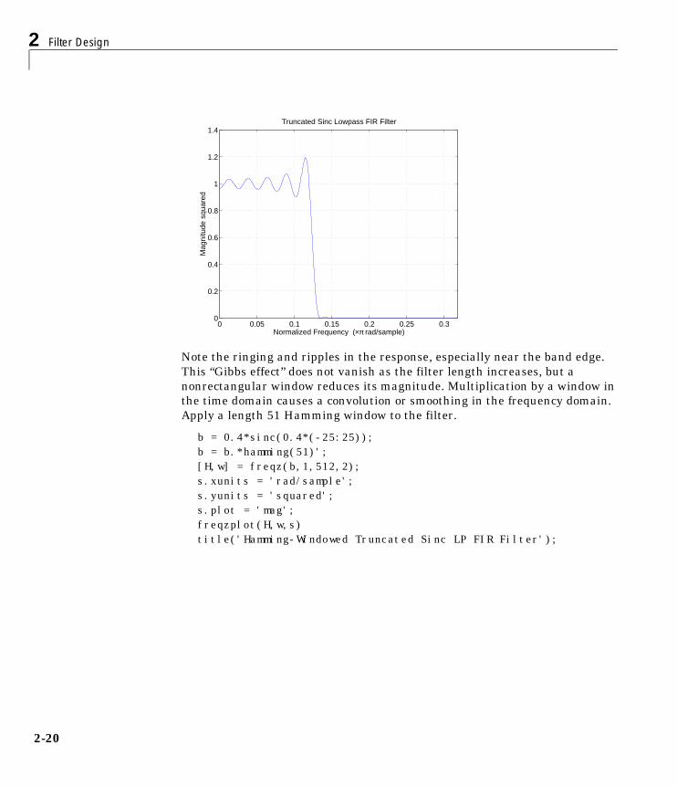
2 Filter Design
2-20
Note the ringing and ripples in the response, especially near the band edge.This “Gibbs effect” does not vanish as the filter length increases, but anonrectangular window reduces its magnitude. Multiplication by a window inthe time domain causes a convolution or smoothing in the frequency domain.Apply a length 51 Hamming window to the filter.
b = 0.4*sinc(0.4*(-25:25));b = b.*hamming(51)';[H,w] = freqz(b,1,512,2);s.xunits = 'rad/sample';s.yunits = 'squared';s.plot = 'mag';freqzplot(H,w,s)title('Hamming-Windowed Truncated Sinc LP FIR Filter');
0 0.05 0.1 0.15 0.2 0.25 0.30
0.2
0.4
0.6
0.8
1
1.2
1.4
Normalized Frequency (×π rad/sample)
Mag
nitu
de s
quar
ed
Truncated Sinc Lowpass FIR Filter
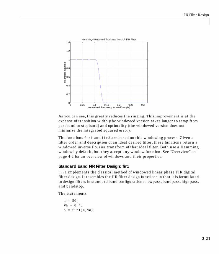
FIR Filter Design
2-21
As you can see, this greatly reduces the ringing. This improvement is at theexpense of transition width (the windowed version takes longer to ramp frompassband to stopband) and optimality (the windowed version does notminimize the integrated squared error).
The functions fir1 and fir2 are based on this windowing process. Given afilter order and description of an ideal desired filter, these functions return awindowed inverse Fourier transform of that ideal filter. Both use a Hammingwindow by default, but they accept any window function. See “Overview” onpage 4-2 for an overview of windows and their properties.
Standard Band FIR Filter Design: fir1fir1 implements the classical method of windowed linear phase FIR digitalfilter design. It resembles the IIR filter design functions in that it is formulatedto design filters in standard band configurations: lowpass, bandpass, highpass,and bandstop.
The statements
n = 50;Wn = 0.4;b = fir1(n,Wn);
0 0.05 0.1 0.15 0.2 0.25 0.30
0.2
0.4
0.6
0.8
1
1.2
1.4
Normalized Frequency (×π rad/sample)
Mag
nitu
de s
quar
ed
Hamming−Windowed Truncated Sinc LP FIR Filter
2 Filter Design
2-22
create row vector b containing the coefficients of the order nHamming-windowed filter. This is a lowpass, linear phase FIR filter with cutofffrequency Wn. Wn is a number between 0 and 1, where 1 corresponds to theNyquist frequency, half the sampling frequency. (Unlike other methods, hereWn corresponds to the 6 dB point.) For a highpass filter, simply append thestring 'high' to the function’s parameter list. For a bandpass or bandstopfilter, specify Wn as a two-element vector containing the passband edgefrequencies; append the string 'stop' for the bandstop configuration.
b = fir1(n,Wn,window) uses the window specified in column vector window forthe design. The vector window must be n+1 elements long. If you do not specifya window, fir1 applies a Hamming window.
Kaiser Window Order Estimation. The kaiserord function estimates the filterorder, cutoff frequency, and Kaiser window beta parameter needed to meet agiven set of specifications. Given a vector of frequency band edges and acorresponding vector of magnitudes, as well as maximum allowable ripple,kaiserord returns appropriate input parameters for the fir1 function.
Multiband FIR Filter Design: fir2The fir2 function also designs windowed FIR filters, but with an arbitrarilyshaped piecewise linear frequency response. This is in contrast to fir1, whichonly designs filters in standard lowpass, highpass, bandpass, and bandstopconfigurations.
The commands
n = 50;f = [0 .4 .5 1];m = [1 1 0 0];b = fir2(n,f,m);
return row vector b containing the n+1 coefficients of the order n FIR filterwhose frequency-magnitude characteristics match those given by vectors fand m. f is a vector of frequency points ranging from 0 to 1, where 1 representsthe Nyquist frequency. m is a vector containing the desired magnitude responseat the points specified in f. (The IIR counterpart of this function is yulewalk,which also designs filters based on arbitrary piecewise linear magnituderesponses. See “IIR Filter Design” on page 2-5 for details.)
FIR Filter Design
2-23
Multiband FIR Filter Design with Transition BandsThe firls and remez functions provide a more general means of specifying theideal desired filter than the fir1 and fir2 functions. These functions designHilbert transformers, differentiators, and other filters with odd symmetriccoefficients (type III and type IV linear phase). They also let you includetransition or “don’t care” regions in which the error is not minimized, andperform band dependent weighting of the minimization.
The firls function is an extension of the fir1 and fir2 functions in that itminimizes the integral of the square of the error between the desired frequencyresponse and the actual frequency response.
The remez function implements the Parks-McClellan algorithm, which usesthe Remez exchange algorithm and Chebyshev approximation theory to designfilters with optimal fits between the desired and actual frequency responses.The filters are optimal in the sense that they minimize the maximum errorbetween the desired frequency response and the actual frequency response;they are sometimes called minimax filters. Filters designed in this way exhibitan equiripple behavior in their frequency response, and hence are also knownas equiripple filters. The Parks-McClellan FIR filter design algorithm isperhaps the most popular and widely used FIR filter design methodology.
The syntax for firls and remez is the same; the only difference is theirminimization schemes. The next example shows how filters designed withfirls and remez reflect these different schemes.
Basic ConfigurationsThe default mode of operation of firls and remez is to design type I or type IIlinear phase filters, depending on whether the order you desire is even or odd,respectively. A lowpass example with approximate amplitude 1 from 0 to0.4 Hz, and approximate amplitude 0 from 0.5 to 1.0 Hz is
n = 20; % Filter orderf = [0 0.4 0.5 1]; % Frequency band edgesa = [1 1 0 0]; % Desired amplitudesb = remez(n,f,a);
From 0.4 to 0.5 Hz, remez performs no error minimization; this is a transitionband or “don’t care” region. A transition band minimizes the error more in thebands that you do care about, at the expense of a slower transition rate. In this
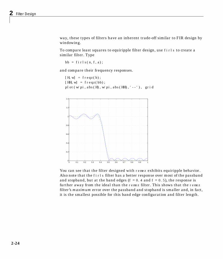
2 Filter Design
2-24
way, these types of filters have an inherent trade-off similar to FIR design bywindowing.
To compare least squares to equiripple filter design, use firls to create asimilar filter. Type
bb = firls(n,f,a);
and compare their frequency responses.
[H,w] = freqz(b);[HH,w] = freqz(bb);plot(w/pi,abs(H),w/pi,abs(HH),'--'), grid
You can see that the filter designed with remez exhibits equiripple behavior.Also note that the firls filter has a better response over most of the passbandand stopband, but at the band edges (f = 0.4 and f = 0.5), the response isfurther away from the ideal than the remez filter. This shows that the remezfilter’s maximum error over the passband and stopband is smaller and, in fact,it is the smallest possible for this band edge configuration and filter length.
0 0.1 0.2 0.3 0.4 0.5 0.6 0.7 0.8 0.9 10
0.2
0.4
0.6
0.8
1
1.2
1.4

FIR Filter Design
2-25
Think of frequency bands as lines over short frequency intervals. remez andfirls use this scheme to represent any piecewise linear desired function withany transition bands. firls and remez design lowpass, highpass, bandpass,and bandstop filters; a bandpass example is
f = [0 0.3 0.4 0.7 0.8 1]; % Band edges in pairsa = [0 0 1 1 0 0]; % Bandpass filter amplitude
Technically, these f and a vectors define five bands:
• Two stopbands, from 0.0 to 0.3 and from 0.8 to 1.0
• A passband from 0.4 to 0.7
• Two transition bands, from 0.3 to 0.4 and from 0.7 to 0.8
Example highpass and bandstop filters are
f = [0 0.7 0.8 1]; % Band edges in pairsa = [0 0 1 1]; % Highpass filter amplitude
f = [0 0.3 0.4 0.5 0.8 1]; % Band edges in pairsa = [1 1 0 0 1 1]; % Bandstop filter amplitude
An example multiband bandpass filter is
f = [0 0.1 0.15 0.25 0.3 0.4 0.45 0.55 0.6 0.7 0.75 0.85 0.9 1];a = [1 1 0 0 1 1 0 0 1 1 0 0 1 1];
Another possibility is a filter that has as a transition region the line connectingthe passband with the stopband; this can help control “runaway” magnituderesponse in wide transition regions.
f = [0 0.4 0.42 0.48 0.5 1];a = [1 1 0.8 0.2 0 0]; % Passband,linear transition,stopband
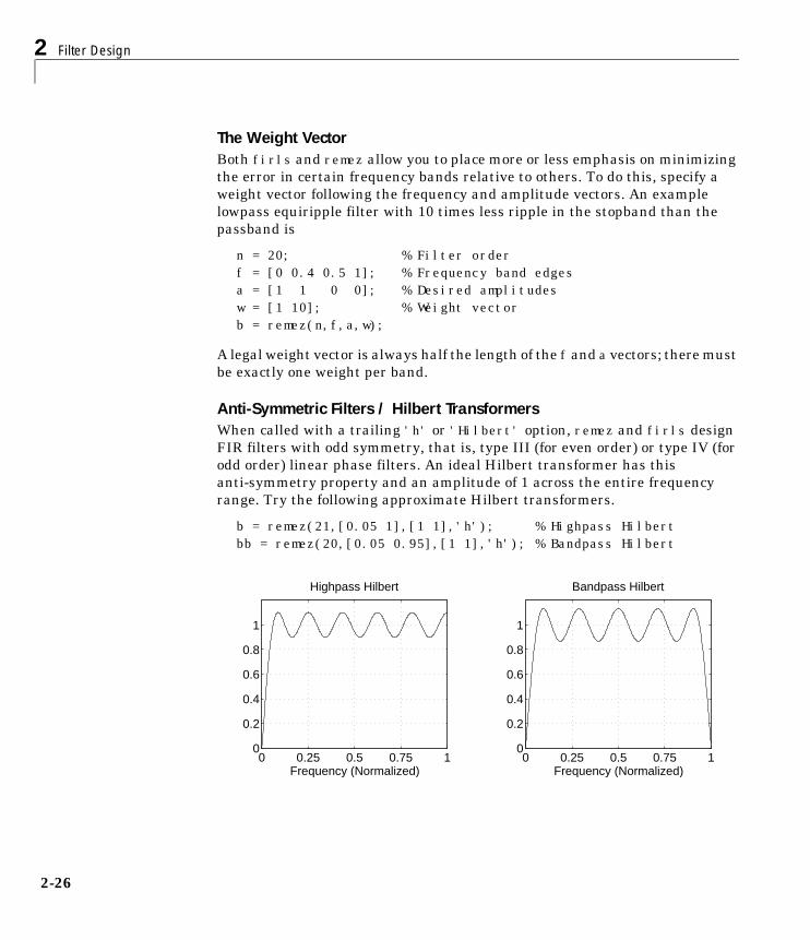
2 Filter Design
2-26
The Weight VectorBoth firls and remez allow you to place more or less emphasis on minimizingthe error in certain frequency bands relative to others. To do this, specify aweight vector following the frequency and amplitude vectors. An examplelowpass equiripple filter with 10 times less ripple in the stopband than thepassband is
n = 20; % Filter orderf = [0 0.4 0.5 1]; % Frequency band edgesa = [1 1 0 0]; % Desired amplitudesw = [1 10]; % Weight vectorb = remez(n,f,a,w);
A legal weight vector is always half the length of the f and a vectors; there mustbe exactly one weight per band.
Anti-Symmetric Filters / Hilbert TransformersWhen called with a trailing 'h' or 'Hilbert' option, remez and firls designFIR filters with odd symmetry, that is, type III (for even order) or type IV (forodd order) linear phase filters. An ideal Hilbert transformer has thisanti-symmetry property and an amplitude of 1 across the entire frequencyrange. Try the following approximate Hilbert transformers.
b = remez(21,[0.05 1],[1 1],'h'); % Highpass Hilbertbb = remez(20,[0.05 0.95],[1 1],'h'); % Bandpass Hilbert
0 0.25 0.5 0.75 10
0.2
0.4
0.6
0.8
1
Frequency (Normalized)
Bandpass Hilbert
0 0.25 0.5 0.75 10
0.2
0.4
0.6
0.8
1
Frequency (Normalized)
Highpass Hilbert
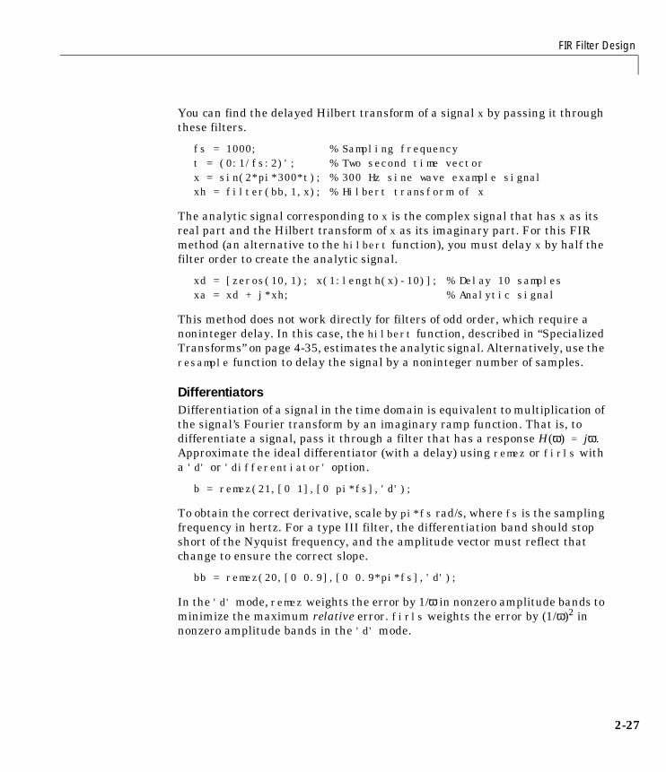
FIR Filter Design
2-27
You can find the delayed Hilbert transform of a signal x by passing it throughthese filters.
fs = 1000; % Sampling frequencyt = (0:1/fs:2)'; % Two second time vectorx = sin(2*pi*300*t); % 300 Hz sine wave example signalxh = filter(bb,1,x); % Hilbert transform of x
The analytic signal corresponding to x is the complex signal that has x as itsreal part and the Hilbert transform of x as its imaginary part. For this FIRmethod (an alternative to the hilbert function), you must delay x by half thefilter order to create the analytic signal.
xd = [zeros(10,1); x(1:length(x)-10)]; % Delay 10 samplesxa = xd + j*xh; % Analytic signal
This method does not work directly for filters of odd order, which require anoninteger delay. In this case, the hilbert function, described in “SpecializedTransforms” on page 4-35, estimates the analytic signal. Alternatively, use theresample function to delay the signal by a noninteger number of samples.
DifferentiatorsDifferentiation of a signal in the time domain is equivalent to multiplication ofthe signal’s Fourier transform by an imaginary ramp function. That is, todifferentiate a signal, pass it through a filter that has a response H(ω) = jω.Approximate the ideal differentiator (with a delay) using remez or firls witha 'd' or 'differentiator' option.
b = remez(21,[0 1],[0 pi*fs],'d');
To obtain the correct derivative, scale by pi*fs rad/s, where fs is the samplingfrequency in hertz. For a type III filter, the differentiation band should stopshort of the Nyquist frequency, and the amplitude vector must reflect thatchange to ensure the correct slope.
bb = remez(20,[0 0.9],[0 0.9*pi*fs],'d');
In the 'd' mode, remez weights the error by 1/ω in nonzero amplitude bands tominimize the maximum relative error. firls weights the error by (1/ω)2 innonzero amplitude bands in the 'd' mode.
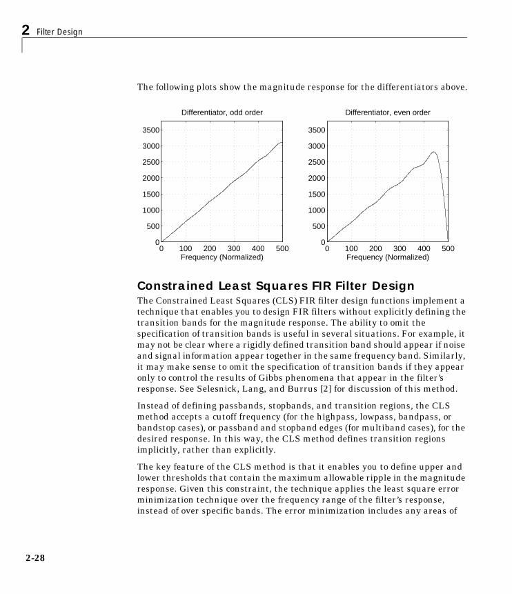
2 Filter Design
2-28
The following plots show the magnitude response for the differentiators above.
Constrained Least Squares FIR Filter DesignThe Constrained Least Squares (CLS) FIR filter design functions implement atechnique that enables you to design FIR filters without explicitly defining thetransition bands for the magnitude response. The ability to omit thespecification of transition bands is useful in several situations. For example, itmay not be clear where a rigidly defined transition band should appear if noiseand signal information appear together in the same frequency band. Similarly,it may make sense to omit the specification of transition bands if they appearonly to control the results of Gibbs phenomena that appear in the filter’sresponse. See Selesnick, Lang, and Burrus [2] for discussion of this method.
Instead of defining passbands, stopbands, and transition regions, the CLSmethod accepts a cutoff frequency (for the highpass, lowpass, bandpass, orbandstop cases), or passband and stopband edges (for multiband cases), for thedesired response. In this way, the CLS method defines transition regionsimplicitly, rather than explicitly.
The key feature of the CLS method is that it enables you to define upper andlower thresholds that contain the maximum allowable ripple in the magnituderesponse. Given this constraint, the technique applies the least square errorminimization technique over the frequency range of the filter’s response,instead of over specific bands. The error minimization includes any areas of
0 100 200 300 400 5000
500
1000
1500
2000
2500
3000
3500
Differentiator, odd order
Frequency (Normalized)0 100 200 300 400 500
0
500
1000
1500
2000
2500
3000
3500
Differentiator, even order
Frequency (Normalized)

FIR Filter Design
2-29
discontinuity in the ideal, “brick wall” response. An additional benefit is thatthe technique enables you to specify arbitrarily small peaks resulting fromGibbs’ phenomena.
There are two toolbox functions that implement this design technique.
For details on the calling syntax for these functions, see their referencedescriptions in Chapter 7, “Function Reference.”
Basic Lowpass and Highpass CLS Filter DesignThe most basic of the CLS design functions, fircls1, uses this technique todesign lowpass and highpass FIR filters. As an example, consider designing afilter with order 61 impulse response and cutoff frequency of 0.3 (normalized).Further, define the upper and lower bounds that constrain the design processas:
• Maximum passband deviation from 1 (passband ripple) of 0.02.
• Maximum stopband deviation from 0 (stopband ripple) of 0.008.
To approach this design problem using fircls1, use the following commands.
n = 61;wo = 0.3;dp = 0.02;ds = 0.008;h = fircls1(n,wo,dp,ds,'plot');
Description Function
Constrained least square multiband FIR filter design fircls
Constrained least square filter design for lowpass andhighpass linear phase filters
fircls1
0 ds = 0.0081dp = 0.02
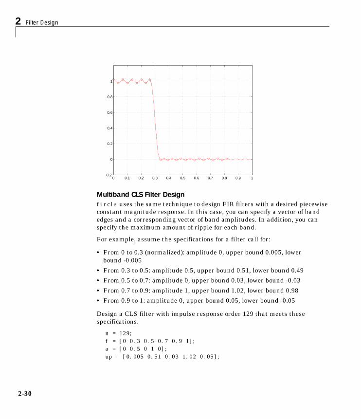
2 Filter Design
2-30
Multiband CLS Filter Designfircls uses the same technique to design FIR filters with a desired piecewiseconstant magnitude response. In this case, you can specify a vector of bandedges and a corresponding vector of band amplitudes. In addition, you canspecify the maximum amount of ripple for each band.
For example, assume the specifications for a filter call for:
• From 0 to 0.3 (normalized): amplitude 0, upper bound 0.005, lowerbound -0.005
• From 0.3 to 0.5: amplitude 0.5, upper bound 0.51, lower bound 0.49
• From 0.5 to 0.7: amplitude 0, upper bound 0.03, lower bound -0.03
• From 0.7 to 0.9: amplitude 1, upper bound 1.02, lower bound 0.98
• From 0.9 to 1: amplitude 0, upper bound 0.05, lower bound -0.05
Design a CLS filter with impulse response order 129 that meets thesespecifications.
n = 129;f = [0 0.3 0.5 0.7 0.9 1];a = [0 0.5 0 1 0];up = [0.005 0.51 0.03 1.02 0.05];
0 0.1 0.2 0.3 0.4 0.5 0.6 0.7 0.8 0.9 1-0.2
0
0.2
0.4
0.6
0.8
1
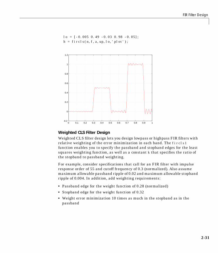
FIR Filter Design
2-31
lo = [-0.005 0.49 -0.03 0.98 -0.05];h = fircls(n,f,a,up,lo,'plot');
Weighted CLS Filter DesignWeighted CLS filter design lets you design lowpass or highpass FIR filters withrelative weighting of the error minimization in each band. The fircls1function enables you to specify the passband and stopband edges for the leastsquares weighting function, as well as a constant k that specifies the ratio ofthe stopband to passband weighting.
For example, consider specifications that call for an FIR filter with impulseresponse order of 55 and cutoff frequency of 0.3 (normalized). Also assumemaximum allowable passband ripple of 0.02 and maximum allowable stopbandripple of 0.004. In addition, add weighting requirements:
• Passband edge for the weight function of 0.28 (normalized)
• Stopband edge for the weight function of 0.32
• Weight error minimization 10 times as much in the stopband as in thepassband
0 0.1 0.2 0.3 0.4 0.5 0.6 0.7 0.8 0.9 1-0.2
0
0.2
0.4
0.6
0.8
1
1.2
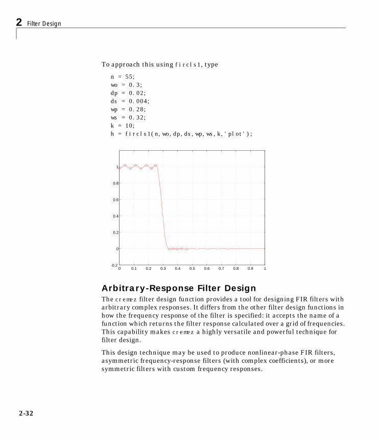
2 Filter Design
2-32
To approach this using fircls1, type
n = 55;wo = 0.3;dp = 0.02;ds = 0.004;wp = 0.28;ws = 0.32;k = 10;h = fircls1(n,wo,dp,ds,wp,ws,k,'plot');
Arbitrary-Response Filter DesignThe cremez filter design function provides a tool for designing FIR filters witharbitrary complex responses. It differs from the other filter design functions inhow the frequency response of the filter is specified: it accepts the name of afunction which returns the filter response calculated over a grid of frequencies.This capability makes cremez a highly versatile and powerful technique forfilter design.
This design technique may be used to produce nonlinear-phase FIR filters,asymmetric frequency-response filters (with complex coefficients), or moresymmetric filters with custom frequency responses.
0 0.1 0.2 0.3 0.4 0.5 0.6 0.7 0.8 0.9 1-0.2
0
0.2
0.4
0.6
0.8
1
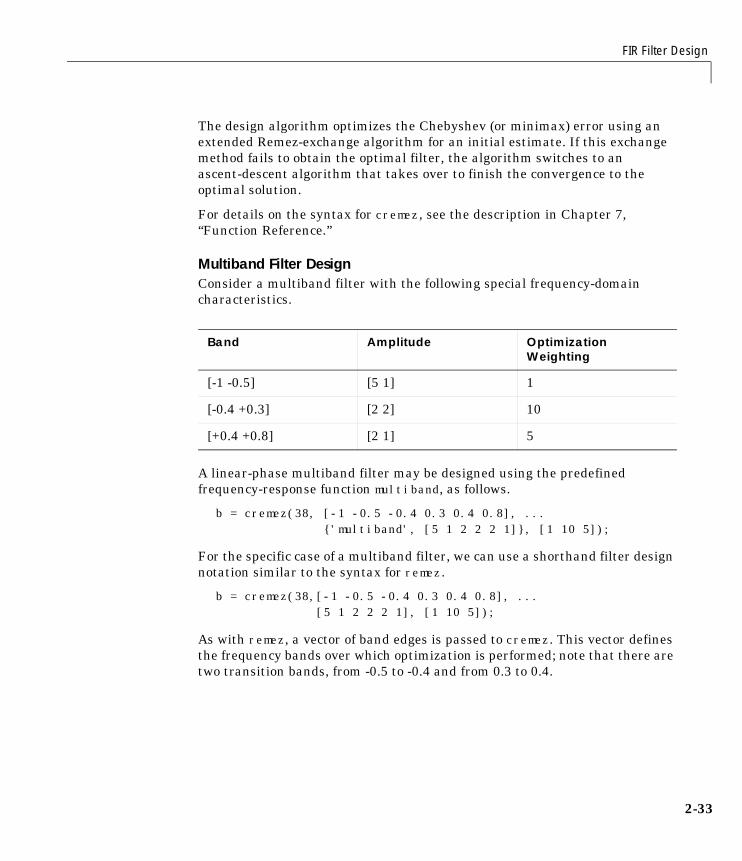
FIR Filter Design
2-33
The design algorithm optimizes the Chebyshev (or minimax) error using anextended Remez-exchange algorithm for an initial estimate. If this exchangemethod fails to obtain the optimal filter, the algorithm switches to anascent-descent algorithm that takes over to finish the convergence to theoptimal solution.
For details on the syntax for cremez, see the description in Chapter 7,“Function Reference.”
Multiband Filter DesignConsider a multiband filter with the following special frequency-domaincharacteristics.
A linear-phase multiband filter may be designed using the predefinedfrequency-response function multiband, as follows.
b = cremez(38, [-1 -0.5 -0.4 0.3 0.4 0.8], ... 'multiband', [5 1 2 2 2 1], [1 10 5]);
For the specific case of a multiband filter, we can use a shorthand filter designnotation similar to the syntax for remez.
b = cremez(38,[-1 -0.5 -0.4 0.3 0.4 0.8], ... [5 1 2 2 2 1], [1 10 5]);
As with remez, a vector of band edges is passed to cremez. This vector definesthe frequency bands over which optimization is performed; note that there aretwo transition bands, from -0.5 to -0.4 and from 0.3 to 0.4.
Band Amplitude Optimization Weighting
[-1 -0.5] [5 1] 1
[-0.4 +0.3] [2 2] 10
[+0.4 +0.8] [2 1] 5

2 Filter Design
2-34
In either case, the frequency response is obtained and plotted using linearscale.
[h,w] = freqz(b,1,512,'whole');plot(w/pi-1,fftshift(abs(h))); grid;xlabel('Normalized Frequency');ylabel('Magnitude Response');
Note that the frequency response has been calculated over the entirenormalized frequency range [-1 +1] by passing the option 'whole' to freqz. Inorder to plot the negative frequency information in a natural way, the responsehas been “wrapped,” just as FFT data is, using fftshift.
The filter response for this multiband filter is complex, which is expectedbecause of the asymmetry in the frequency domain.
-1 -0.8 -0.6 -0.4 -0.2 0 0.2 0.4 0.6 0.8 11
1.5
2
2.5
3
3.5
4
4.5
5
Normalized Frequency
Mag
nitu
de R
espo
nse
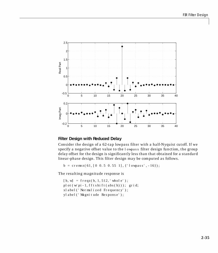
FIR Filter Design
2-35
Filter Design with Reduced DelayConsider the design of a 62-tap lowpass filter with a half-Nyquist cutoff. If wespecify a negative offset value to the lowpass filter design function, the groupdelay offset for the design is significantly less than that obtained for a standardlinear-phase design. This filter design may be computed as follows.
b = cremez(61,[0 0.5 0.55 1],'lowpass',-16);
The resulting magnitude response is
[h,w] = freqz(b,1,512,'whole');plot(w/pi-1,fftshift(abs(h))); grid;xlabel('Normalized Frequency');ylabel('Magnitude Response');
0 5 10 15 20 25 30 35 40-0.5
0
0.5
1
1.5
2
2.5
Rea
l Par
t
0 5 10 15 20 25 30 35 40-0.2
0
0.2
Imag
Par
t
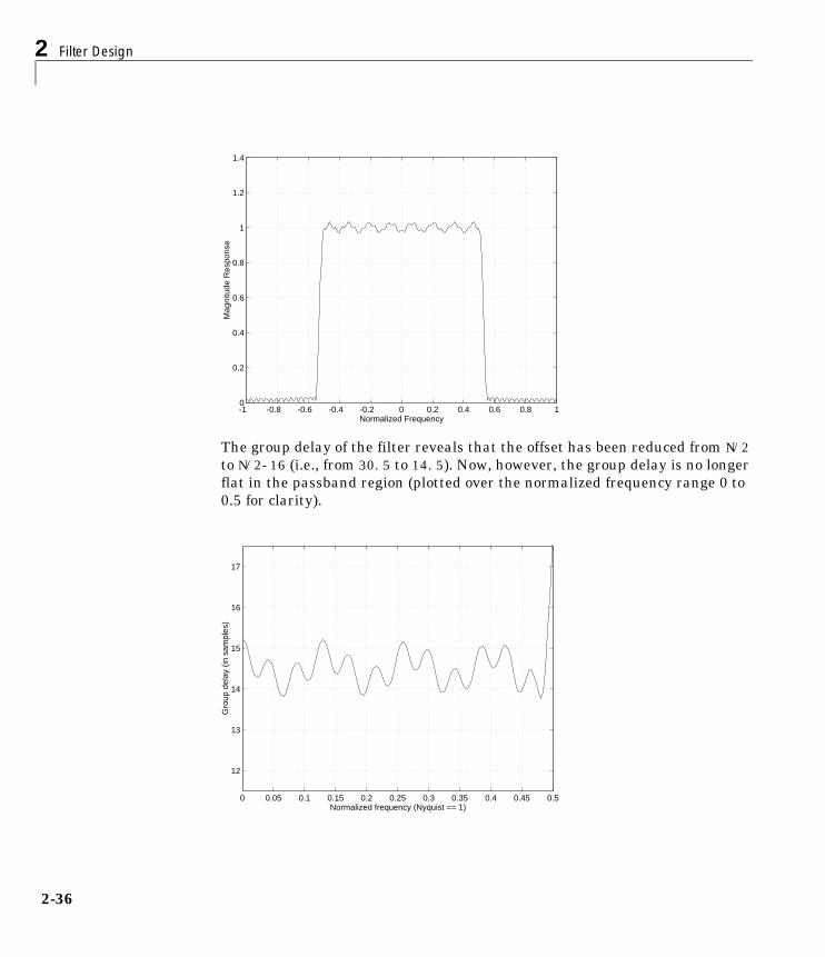
2 Filter Design
2-36
The group delay of the filter reveals that the offset has been reduced from N/2to N/2-16 (i.e., from 30.5 to 14.5). Now, however, the group delay is no longerflat in the passband region (plotted over the normalized frequency range 0 to0.5 for clarity).
-1 -0.8 -0.6 -0.4 -0.2 0 0.2 0.4 0.6 0.8 10
0.2
0.4
0.6
0.8
1
1.2
1.4
Normalized Frequency
Mag
nitu
de R
espo
nse
0 0.05 0.1 0.15 0.2 0.25 0.3 0.35 0.4 0.45 0.5
12
13
14
15
16
17
Normalized frequency (Nyquist == 1)
Gro
up d
elay
(in
sam
ples
)

FIR Filter Design
2-37
If we compare this nonlinear-phase filter to a linear-phase filter that hasexactly 14.5 samples of group delay, the resulting filter is of order 2*14.5, or 29.Using b = cremez(29,[0 0.5 0.55 1],'lowpass'), the passband andstopband ripple is much greater for the order 29 filter. These comparisons canassist you in deciding which filter is more appropriate for a specific application.
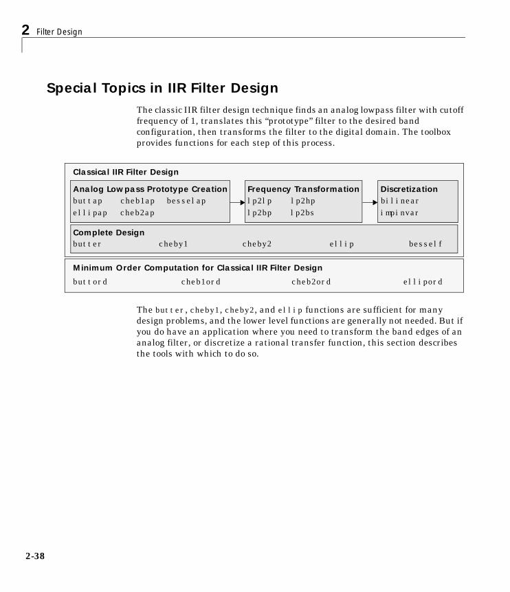
2 Filter Design
2-38
Special Topics in IIR Filter DesignThe classic IIR filter design technique finds an analog lowpass filter with cutofffrequency of 1, translates this “prototype” filter to the desired bandconfiguration, then transforms the filter to the digital domain. The toolboxprovides functions for each step of this process.
The butter, cheby1, cheby2, and ellip functions are sufficient for manydesign problems, and the lower level functions are generally not needed. But ifyou do have an application where you need to transform the band edges of ananalog filter, or discretize a rational transfer function, this section describesthe tools with which to do so.
Classical IIR Filter Design
Analog Lowpass Prototype Creation Frequency Transformation Discretizationbuttapellipap
cheb1apcheb2ap
besselap lp2lplp2bp
lp2hplp2bs
bilinearimpinvar
butter cheby1 cheby2 ellip besself
Minimum Order Computation for Classical IIR Filter Design
buttord cheb1ord cheb2ord ellipord
Complete Design
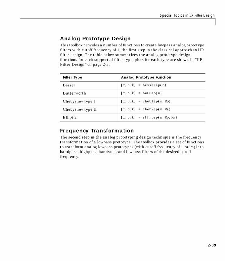
Special Topics in IIR Filter Design
2-39
Analog Prototype DesignThis toolbox provides a number of functions to create lowpass analog prototypefilters with cutoff frequency of 1, the first step in the classical approach to IIRfilter design. The table below summarizes the analog prototype designfunctions for each supported filter type; plots for each type are shown in “IIRFilter Design” on page 2-5.
Frequency TransformationThe second step in the analog prototyping design technique is the frequencytransformation of a lowpass prototype. The toolbox provides a set of functionsto transform analog lowpass prototypes (with cutoff frequency of 1 rad/s) intobandpass, highpass, bandstop, and lowpass filters of the desired cutofffrequency.
Filter Type Analog Prototype Function
Bessel [z,p,k] = besselap(n)
Butterworth [z,p,k] = buttap(n)
Chebyshev type I [z,p,k] = cheb1ap(n,Rp)
Chebyshev type II [z,p,k] = cheb2ap(n,Rs)
Elliptic [z,p,k] = ellipap(n,Rp,Rs)

2 Filter Design
2-40
As shown, all of the frequency transformation functions can accept two linearsystem models: transfer function and state-space form. For the bandpass andbandstop cases
and
where ω1 is the lower band edge and ω2 is the upper band edge.
The frequency transformation functions perform frequency variablesubstitution. In the case of lp2bp and lp2bs, this is a second-ordersubstitution, so the output filter is twice the order of the input. For lp2lp andlp2hp, the output filter is the same order as the input.
To begin designing an order 10 bandpass Chebyshev type I filter with a valueof 3 dB for passband ripple, enter
[z,p,k] = cheb1ap(5,3);
Freq. Transformation Transformation Function
Lowpass to lowpass [numt,dent] = lp2lp(num,den,Wo)[At,Bt,Ct,Dt] = lp2lp(A,B,C,D,Wo)
Lowpass to highpass [numt,dent] = lp2hp(num,den,Wo)[At,Bt,Ct,Dt] = lp2hp(A,B,C,D,Wo)
Lowpass to bandpass [numt,dent] = lp2bp(num,den,Wo,Bw)[At,Bt,Ct,Dt] = lp2bp(A,B,C,D,Wo,Bw)
Lowpass to bandstop [numt,dent] = lp2bs(num,den,Wo,Bw)[At,Bt,Ct,Dt] = lp2bs(A,B,C,D,Wo,Bw)
s' s ω0⁄=
s'ω0s
-------=
s'ω0Bω-------
s ω0⁄( )2 1+
s ω0⁄-------------------------------=
s'Bωω0-------
s ω0⁄
s ω0⁄( )2 1+-------------------------------=
ω0 ω1ω2=
Bω ω2 ω1–=

Special Topics in IIR Filter Design
2-41
Outputs z, p, and k contain the zeros, poles, and gain of a lowpass analog filterwith cutoff frequency Ωc equal to 1 rad/s. Use the lp2bp function to transformthis lowpass prototype to a bandpass analog filter with band edgesand . First, convert the filter to state-space form so the lp2bp functioncan accept it.
[A,B,C,D] = zp2ss(z,p,k); % Convert to state-space form.
Now, find the bandwidth and center frequency, and call lp2bp.
u1 = 0.1*2*pi; u2 = 0.5*2*pi; % In radians per secondBw = u2-u1;Wo = sqrt(u1*u2);[At,Bt,Ct,Dt] = lp2bp(A,B,C,D,Wo,Bw);
Finally, calculate the frequency response and plot its magnitude.
[b,a] = ss2tf(At,Bt,Ct,Dt); % Convert to TF form.w = linspace(0.01,1,500)*2*pi; % Generate frequency vector.h = freqs(b,a,w); % Compute frequency response.semilogy(w/2/pi,abs(h)), grid % Plot log magnitude vs. freq.xlabel('Frequency (Hz)');
.
Ω1 π 5⁄=Ω2 π=
0 0.2 0.4 0.6 0.8 110
−7
10−6
10−5
10−4
10−3
10−2
10−1
100
Frequency (Hz)
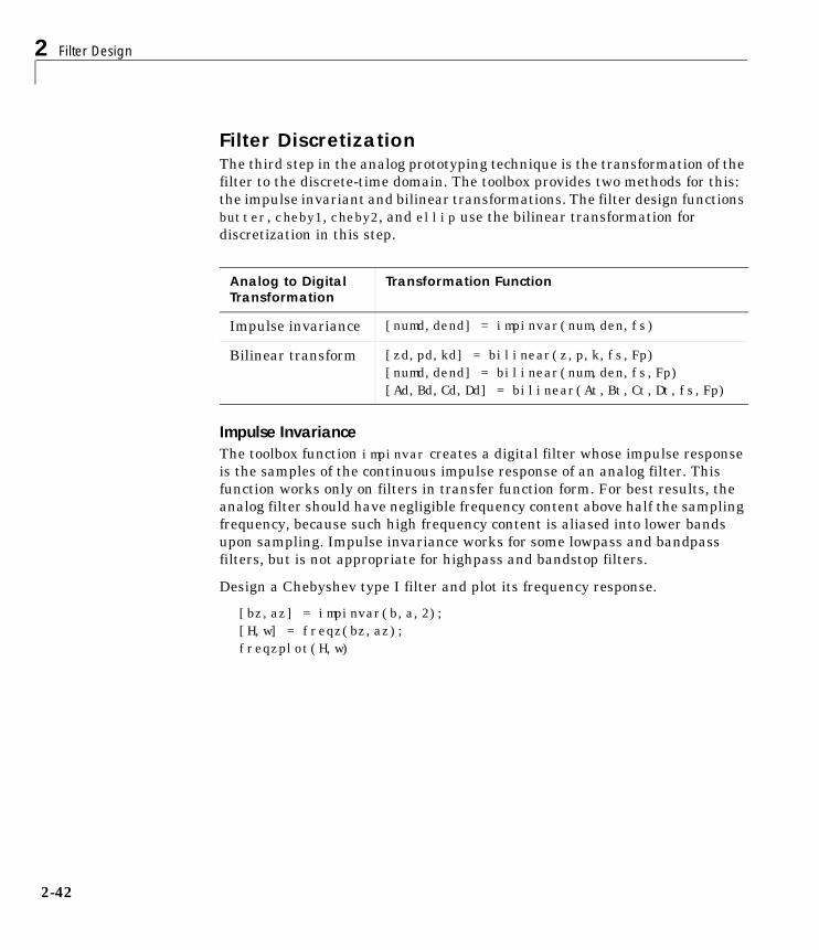
2 Filter Design
2-42
Filter DiscretizationThe third step in the analog prototyping technique is the transformation of thefilter to the discrete-time domain. The toolbox provides two methods for this:the impulse invariant and bilinear transformations. The filter design functionsbutter, cheby1, cheby2, and ellip use the bilinear transformation fordiscretization in this step.
Impulse InvarianceThe toolbox function impinvar creates a digital filter whose impulse responseis the samples of the continuous impulse response of an analog filter. Thisfunction works only on filters in transfer function form. For best results, theanalog filter should have negligible frequency content above half the samplingfrequency, because such high frequency content is aliased into lower bandsupon sampling. Impulse invariance works for some lowpass and bandpassfilters, but is not appropriate for highpass and bandstop filters.
Design a Chebyshev type I filter and plot its frequency response.
[bz,az] = impinvar(b,a,2);[H,w] = freqz(bz,az);freqzplot(H,w)
Analog to Digital Transformation
Transformation Function
Impulse invariance [numd,dend] = impinvar(num,den,fs)
Bilinear transform [zd,pd,kd] = bilinear(z,p,k,fs,Fp)[numd,dend] = bilinear(num,den,fs,Fp)[Ad,Bd,Cd,Dd] = bilinear(At,Bt,Ct,Dt,fs,Fp)
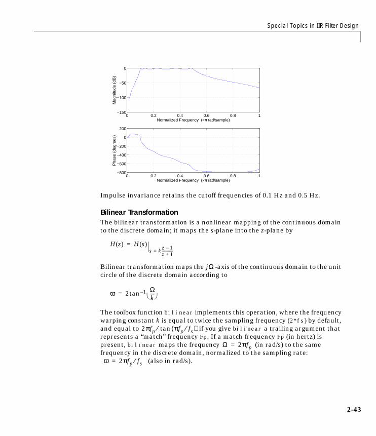
Special Topics in IIR Filter Design
2-43
Impulse invariance retains the cutoff frequencies of 0.1 Hz and 0.5 Hz.
Bilinear TransformationThe bilinear transformation is a nonlinear mapping of the continuous domainto the discrete domain; it maps the s-plane into the z-plane by
Bilinear transformation maps the -axis of the continuous domain to the unitcircle of the discrete domain according to
The toolbox function bilinear implements this operation, where the frequencywarping constant k is equal to twice the sampling frequency (2*fs) by default,and equal to if you give bilinear a trailing argument thatrepresents a “match” frequency Fp. If a match frequency Fp (in hertz) ispresent, bilinear maps the frequency (in rad/s) to the samefrequency in the discrete domain, normalized to the sampling rate:
(also in rad/s).
0 0.2 0.4 0.6 0.8 1−800
−600
−400
−200
0
200
Normalized Frequency (×π rad/sample)
Pha
se (
degr
ees)
0 0.2 0.4 0.6 0.8 1−150
−100
−50
0
Normalized Frequency (×π rad/sample)
Mag
nitu
de (
dB)
H z( ) H s( )s kz 1–
z 1+------------=
=
jΩ
ω 2tan 1– Ωk---- =
2πfp πfp fs⁄( )tan⁄
Ω 2πfp=
ω 2πfp fs⁄=
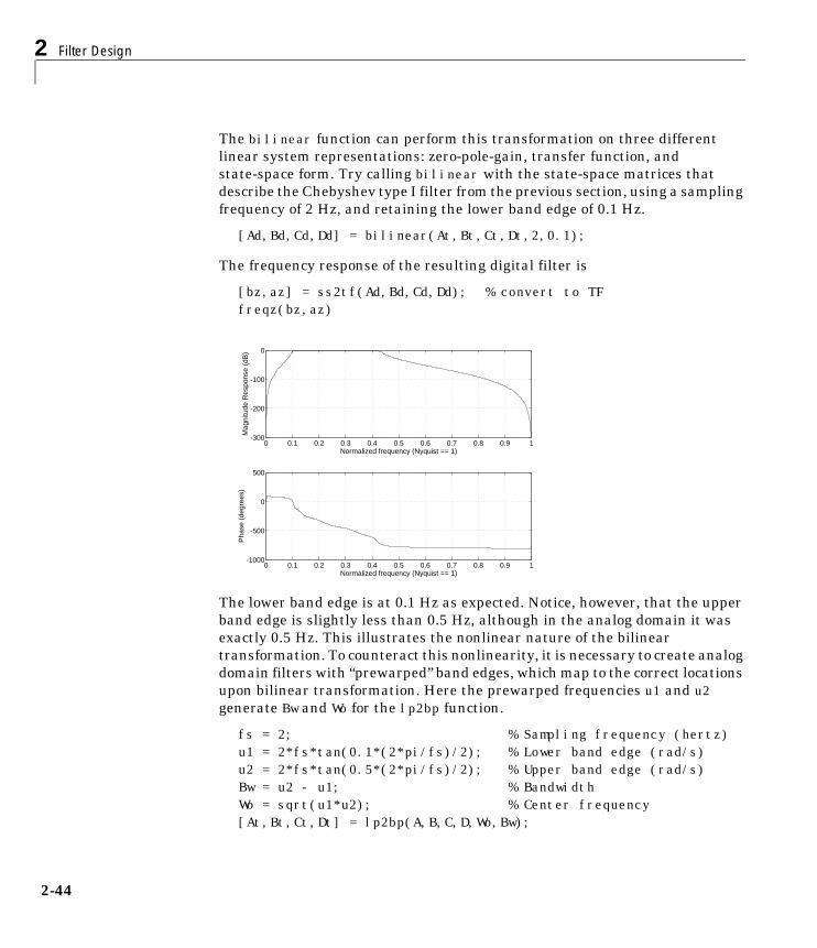
2 Filter Design
2-44
The bilinear function can perform this transformation on three differentlinear system representations: zero-pole-gain, transfer function, andstate-space form. Try calling bilinear with the state-space matrices thatdescribe the Chebyshev type I filter from the previous section, using a samplingfrequency of 2 Hz, and retaining the lower band edge of 0.1 Hz.
[Ad,Bd,Cd,Dd] = bilinear(At,Bt,Ct,Dt,2,0.1);
The frequency response of the resulting digital filter is
[bz,az] = ss2tf(Ad,Bd,Cd,Dd); % convert to TFfreqz(bz,az)
The lower band edge is at 0.1 Hz as expected. Notice, however, that the upperband edge is slightly less than 0.5 Hz, although in the analog domain it wasexactly 0.5 Hz. This illustrates the nonlinear nature of the bilineartransformation. To counteract this nonlinearity, it is necessary to create analogdomain filters with “prewarped” band edges, which map to the correct locationsupon bilinear transformation. Here the prewarped frequencies u1 and u2generate Bw and Wo for the lp2bp function.
fs = 2; % Sampling frequency (hertz)u1 = 2*fs*tan(0.1*(2*pi/fs)/2); % Lower band edge (rad/s)u2 = 2*fs*tan(0.5*(2*pi/fs)/2); % Upper band edge (rad/s)Bw = u2 - u1; % BandwidthWo = sqrt(u1*u2); % Center frequency[At,Bt,Ct,Dt] = lp2bp(A,B,C,D,Wo,Bw);
0 0.1 0.2 0.3 0.4 0.5 0.6 0.7 0.8 0.9 1-1000
-500
0
500
Normalized frequency (Nyquist == 1)
Pha
se (
degr
ees)
0 0.1 0.2 0.3 0.4 0.5 0.6 0.7 0.8 0.9 1-300
-200
-100
0
Normalized frequency (Nyquist == 1)
Mag
nitu
de R
espo
nse
(dB
)

Special Topics in IIR Filter Design
2-45
A digital bandpass filter with correct band edges 0.1 and 0.5 times the Nyquistfrequency is
[Ad,Bd,Cd,Dd] = bilinear(At,Bt,Ct,Dt,fs);
The example bandpass filters from the last two sections could also be createdin one statement using the complete IIR design function cheby1. For instance,an analog version of the example Chebyshev filter is
[b,a] = cheby1(5,3,[0.1 0.5]*2*pi,'s');
Note that the band edges are in rad/s for analog filters, whereas for the digitalcase, frequency is normalized (the Nyquist frequency is equal to 1 Hz).
[bz,az] = cheby1(5,3,[0.1 0.5]);
All of the complete design functions call bilinear internally. They prewarp theband edges as needed to obtain the correct digital filter. See Chapter 7,“Function Reference,” for more on these functions.

2 Filter Design
2-46
Selected Bibliography[1] Karam, L.J., and J.H. McClellan. “Complex Chebyshev Approximation forFIR Filter Design.” IEEE Trans. on Circuits and Systems II. March 1995.
[2] Selesnick, I.W., and C.S. Burrus. “Generalized Digital Butterworth FilterDesign.” Proceedings of the IEEE Int. Conf. Acoust., Speech, Signal Processing.Vol. 3 (May 1996).
[3] Selesnick, I.W., M. Lang, and C.S. Burrus. “Constrained Least SquareDesign of FIR Filters without Specified Transition Bands.” Proceedings of theIEEE Int. Conf. Acoust., Speech, Signal Processing. Vol. 2 (May 1995).Pgs. 1260-1263.
3Statistical SignalProcessing
Overview . . . . . . . . . . . . . . . . . . . . . 3-2
Correlation and Covariance . . . . . . . . . . . . . 3-3Bias and Normalization . . . . . . . . . . . . . . . . 3-4Multiple Channels . . . . . . . . . . . . . . . . . . 3-5
Spectral Analysis . . . . . . . . . . . . . . . . . . 3-6Spectral Estimation Method Overview . . . . . . . . . . 3-8Nonparametric Methods . . . . . . . . . . . . . . . . 3-10Parametric Methods . . . . . . . . . . . . . . . . . 3-30
Selected Bibliography . . . . . . . . . . . . . . . 3-39

3 Statistical Signal Processing
3-2
OverviewThe Signal Processing Toolbox provides tools for estimating importantfunctions of random signals. In particular, there are tools to estimatecorrelation and covariance sequences and spectral density functions of discretesignals. The following sections explain the correlation and covariance functionsand discuss the mathematically related functions for estimating the powerspectrum:
• “Correlation and Covariance”
• “Spectral Analysis”
• “Selected Bibliography”
Correlation and Covariance
3-3
Correlation and CovarianceThe functions xcorr and xcov estimate the cross-correlation andcross-covariance sequences of random processes. They also handleautocorrelation and autocovariance as special cases.
The true cross-correlation sequence is a statistical quantity defined as
where xn and yn are stationary random processes, , and E⋅ is theexpected value operator. The covariance sequence is the mean-removedcross-correlation sequence
or, in terms of the cross-correlation,
In practice, you must estimate these sequences, because it is possible to accessonly a finite segment of the infinite-length random process. A common estimatebased on N samples of xn and yn is the deterministic cross-correlation sequence(also called the time-ambiguity function)
where we assume for this discussion that xn and yn are indexed from 0 to N-1,and from -(N-1) to N-1. The xcorr function evaluates this sum with anefficient FFT-based algorithm, given inputs xn and yn stored in length Nvectors x and y. Its operation is equivalent to convolution with one of the twosubsequences reversed in time.
For example,
x = [1 1 1 1 1]';y = x;
Rxy m( ) Exn m+ y*n Exny*n m– ==
∞– n ∞< <
Cxy m( ) E xn m+ µx–( ) yn µy–( )*=
Cxy m( ) Rxy m( ) µxµ*y–=
Rxy m( )xn m+ yn
*
n 0=
N m– 1–
m 0≥
Rˆ yx*
m–( ) m 0<
=
Rxy m( )
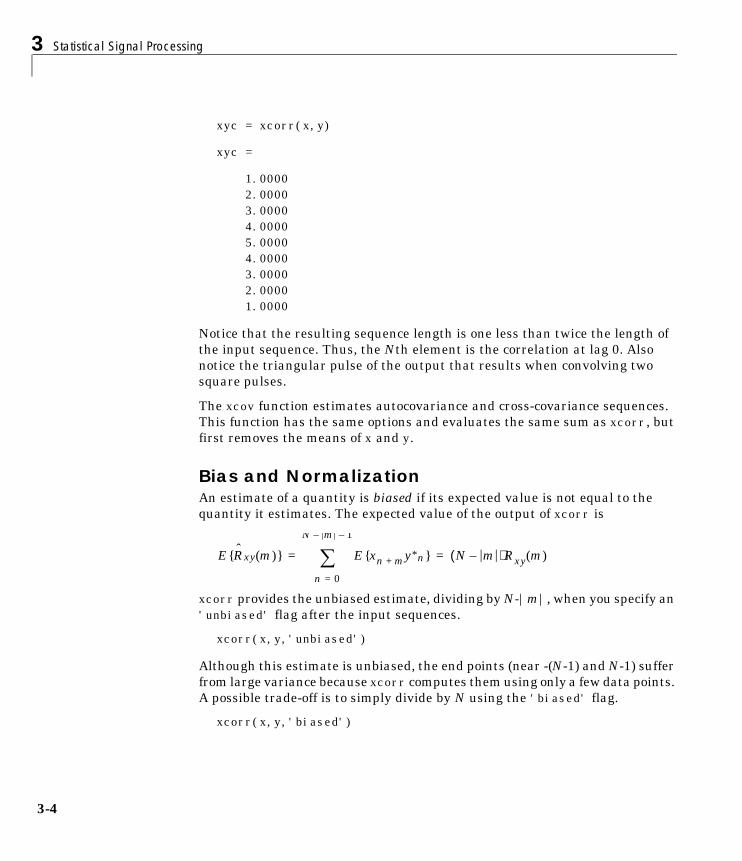
3 Statistical Signal Processing
3-4
xyc = xcorr(x,y)
xyc =
1.0000 2.0000 3.0000 4.0000 5.0000 4.0000 3.0000 2.0000 1.0000
Notice that the resulting sequence length is one less than twice the length ofthe input sequence. Thus, the Nth element is the correlation at lag 0. Alsonotice the triangular pulse of the output that results when convolving twosquare pulses.
The xcov function estimates autocovariance and cross-covariance sequences.This function has the same options and evaluates the same sum as xcorr, butfirst removes the means of x and y.
Bias and NormalizationAn estimate of a quantity is biased if its expected value is not equal to thequantity it estimates. The expected value of the output of xcorr is
xcorr provides the unbiased estimate, dividing by N-|m|, when you specify an'unbiased' flag after the input sequences.
xcorr(x,y,'unbiased')
Although this estimate is unbiased, the end points (near -(N-1) and N-1) sufferfrom large variance because xcorr computes them using only a few data points.A possible trade-off is to simply divide by N using the 'biased' flag.
xcorr(x,y,'biased')
ERxy m( ) Exn m+ y*n
n 0=
N m– 1–
N m–( )Rxy m( )= =
Correlation and Covariance
3-5
With this scheme, only the sample of the correlation at zero lag (the Nth outputelement) is unbiased. This estimate is often more desirable than the unbiasedone because it avoids random large variations at the end points of thecorrelation sequence.
xcorr provides one other normalization scheme. The syntax
xcorr(x,y,'coeff')
divides the output by norm(x)*norm(y) so that, for autocorrelations, thesample at zero lag is 1.
Multiple ChannelsFor a multichannel signal, xcorr and xcov estimate the autocorrelation andcross-correlation and covariance sequences for all of the channels at once. If Sis an M-by-N signal matrix representing N channels in its columns, xcorr(S)returns a (2M-1)-by-N2 matrix with the autocorrelations and cross-correlationsof the channels of S in its N2 columns. If S is a three-channel signal
S = [s1 s2 s3]
then the result of xcorr(S) is organized as
R = [Rs1s1 Rs1s2 Rs1s3 Rs2s1 Rs2s2 Rs2s3 Rs3s1 Rs3s2 Rs3s3]
Two related functions, cov and corrcoef, are available in the standardMATLAB environment. They estimate covariance and normalized covariancerespectively between the different channels at lag 0 and arrange them in asquare matrix.

3 Statistical Signal Processing
3-6
Spectral AnalysisThe goal of spectral estimation is to describe the distribution (over frequency)of the power contained in a signal, based on a finite set of data. Estimation ofpower spectra is useful in a variety of applications, including the detection ofsignals buried in wide-band noise.
The power spectrum of a stationary random process xn is mathematicallyrelated to the correlation sequence by the discrete-time Fourier transform. Interms of normalized frequency, this is given by
This can be written as a function of physical frequency f (e.g., in hertz) by usingthe relation ω = 2πf/fs, where fs is the sampling frequency.
The correlation sequence can be derived from the power spectrum by use of theinverse discrete-time Fourier transform.
The average power of the sequence xn over the entire Nyquist interval isrepresented by
Sxx ω( ) Rxx m( )e jωm–
m ∞–=
∞
=
Sxx f( ) Rxx m( )e 2πjfm– fs⁄
m ∞–=
∞
=
Rxx m( )Sxx ω( )ejωm
2π------------------------------ ωd
π–
π
Sxx f( )e2πjfm fs⁄
fs--------------------------------------- fd
fs 2⁄–
fs 2⁄
= =
Rxx 0( )Sxx ω( )
2π----------------- ωd
π–
π
Sxx f( )
fs--------------- fd
fs 2⁄–
fs 2⁄
= =
Spectral Analysis
3-7
The quantities
from the above expression are defined as the power spectral density (PSD) ofthe stationary random signal xn.
The average power of a signal over a particular frequency band ,, can be found by integrating the PSD over that band.
You can see from the above expression that Pxx(ω) represents the power contentof a signal in an infinitesimal frequency band, which is why we call it the powerspectral density.
The units of the PSD are power (e.g., watts) per unit of frequency. In the caseof Pxx(ω), this is watts/rad/sample or simply watts/rad. In the case of Pxx(f), theunits are watts/hertz. Integration of the PSD with respect to frequency yieldsunits of watts, as expected for the average power .
For real signals, the PSD is symmetric about DC, and thus Pxx(ω) foris sufficient to completely characterize the PSD. However, in order to obtainthe average power over the entire Nyquist interval it is necessary to introducethe concept of the one-sided PSD.
The one-sided PSD is given by
The average power of a signal over the frequency band , ,can be computed using the one-sided PSD as
Pxx ω( )Sxx ω( )
2π-----------------= Pxx f( )
Sxx f( )
fs---------------=and
ω1 ω2[ , ]0 ω1 ω2 π≤<≤
P ω1 ω2,[ ] Pxx ω( ) ωd
ω1
ω2
Pxx ω( ) ωd
ω– 2
ω– 1
+=
P ω1 ω2,[ ]
0 ω π<≤
Ponesided ω( )0 -π ω≤ 0<,2Pxx ω( ) 0 ω≤ π<,
=
ω1 ω2[ , ] 0 ω1 ω2 π≤<≤
P ω1 ω2,[ ] Ponesided ω( ) ωd
ω1
ω2
=

3 Statistical Signal Processing
3-8
Spectral Estimation Method OverviewThe various methods of spectrum estimation available in the Signal ProcessingToolbox can be categorized as follows:
• Nonparametric methods
• Parametric methods
• Subspace methods
Nonparametric methods are those in which the estimate of the PSD is madedirectly from the signal itself. The simplest such method is the periodogram.An improved version of the periodogram is Welch’s method [8]. A more modernnonparametric technique is the multitaper method (MTM).
Parametric methods are those in which the signal whose PSD we want toestimate is assumed to be output of a linear system driven by white noise.Examples are the Yule-Walker autoregressive (AR) method and the Burgmethod. These methods estimate the PSD by first estimating the parameters(coefficients) of the linear system that hypothetically “generates” the signal.They tend to produce better results than classical nonparametric methodswhen the data length of the available signal is relatively short.
Subspace methods, also known as high-resolution methods or super-resolutionmethods, generate frequency component estimates for a signal based on aneigenanalysis or eigendecomposition of the correlation matrix. Examples arethe multiple signal classification (MUSIC) method or the eigenvector (EV)method. These methods are best suited for line spectra – that is, spectra ofsinusoidal signals – and are effective in the detection of sinusoids buried innoise, especially when the signal to noise ratios are low.
All three categories of methods are listed in the table below with thecorresponding toolbox function names. The number below each method nameindicates the page that describes the method in greater detail. See “ParametricModeling” on page 4-11 for details about lpc and other parametric estimationfunctions.

Spectral Analysis
3-9
Method Description Functions
Periodogram(3-10)
Power spectral density estimate periodogram
Welch(3-20)
Averaged periodograms ofoverlapped, windowed signal sections
pwelch, csd,tfe, cohere
Multitaper(3-24)
Spectral estimate from combinationof multiple orthogonal windows (or“tapers”)
pmtm
Yule-Walker AR(3-32)
Autoregressive (AR) spectralestimate of a time-series from itsestimated autocorrelation function
pyulear
Burg(3-33)
Autoregressive (AR) spectralestimation of a time-series byminimization of linear predictionerrors
pburg
Covariance(3-36)
Autoregressive (AR) spectralestimation of a time-series byminimization of the forwardprediction errors
pcov
ModifiedCovariance(3-36)
Autoregressive (AR) spectralestimation of a time-series byminimization of the forward andbackward prediction errors
pmcov
MUSIC(3-36)
Multiple signal classification pmusic
Eigenvector(3-36)
Pseudospectrum estimate peig
3 Statistical Signal Processing
3-10
Nonparametric MethodsThe following sections discuss the periodogram, modified periodogram, Welch,and multitaper methods of nonparametric estimation, along with the relatedCSD function, transfer function estimate, and coherence function.
The PeriodogramOne way of estimating the power spectrum of a process is to simply find thediscrete-time Fourier transform of the samples of the process (usually done ona grid with an FFT) and take the magnitude squared of the result. Thisestimate is called the periodogram.
The periodogram estimate of the PSD of a length-L signal xL[n] is
where
The actual computation of XL(f) can be performed only at a finite number offrequency points, N, and usually employs the FFT. In practice, mostimplementations of the periodogram method compute the N-point PSDestimate
where
It is wise to choose N > L so that N is the next power of two larger than L. Toevaluate XL[fk], we simply pad xL[n] with zeros to length N. If L > N, we mustwrap xL[n] modulo-N prior to computing XL[fk].
Pxx f( )XL f( ) 2
fsL--------------------=
XL f( ) xL n[ ]e2πjfn– fs⁄
n 0=
L 1–
=
Pxx fk[ ]XL fk[ ] 2
fsL-----------------------,= fk
kfsN
--------,= k 0 1 … N 1–, , ,=
XL fk[ ] xL n[ ]e 2πjkn– N⁄
n 0=
N 1–
=
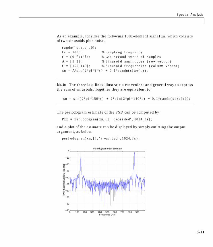
Spectral Analysis
3-11
As an example, consider the following 1001-element signal xn, which consistsof two sinusoids plus noise.
randn('state',0);fs = 1000; % Sampling frequencyt = (0:fs)/fs; % One second worth of samplesA = [1 2]; % Sinusoid amplitudes (row vector)f = [150;140]; % Sinusoid frequencies (column vector)xn = A*sin(2*pi*f*t) + 0.1*randn(size(t));
Note The three last lines illustrate a convenient and general way to expressthe sum of sinusoids. Together they are equivalent to
xn = sin(2*pi*150*t) + 2*sin(2*pi*140*t) + 0.1*randn(size(t));
The periodogram estimate of the PSD can be computed by
Pxx = periodogram(xn,[],'twosided',1024,fs);
and a plot of the estimate can be displayed by simply omitting the outputargument, as below.
periodogram(xn,[],'twosided',1024,fs);
0 100 200 300 400 500 600 700 800 900−90
−80
−70
−60
−50
−40
−30
−20
−10
0
Frequency (Hz)
Pow
er S
pect
ral D
ensi
ty (
dB/H
z)
Periodogram PSD Estimate
3 Statistical Signal Processing
3-12
The average power can be computed by approximating the integral with thefollowing sum.
Pow = (fs/length(Pxx)) * sum(Pxx)
Pow =
2.5028
You can also compute the average power from the one-sided PSD estimate.
Pxxo = periodogram(xn,[],1024,fs);
Pow = (fs/(2*length(Pxxo))) * sum(Pxxo)
Pow =
2.4979
Performance of the PeriodogramThe following sections discuss the performance of the periodogram with regardto the issues of leakage, resolution, bias, and variance.
Spectral Leakage. Consider the power spectrum or PSD of a finite-length signalxL[n], as discussed in “The Periodogram” on page 3-10. It is frequently usefulto interpret xL[n] as the result of multiplying an infinite signal, x[n], by afinite-length rectangular window, wR[n].
Because multiplication in the time domain corresponds to convolution in thefrequency domain, the Fourier transform of the expression above is
The expression developed earlier for the periodogram,
illustrates that the periodogram is also influenced by this convolution.
xL n[ ] x n[ ] wR n[ ]⋅=
XL f( ) 1fs---- X ρ( )WR f ρ–( ) ρd
fs 2⁄–
fs 2⁄
=
Pxx f( )XL f( ) 2
fsL--------------------=

Spectral Analysis
3-13
The effect of the convolution is best understood for sinusoidal data. Supposethat x[n] is composed of a sum of M complex sinusoids.
Its spectrum is
which for a finite-length sequence becomes
So in the spectrum of the finite-length signal, the Dirac deltas have beenreplaced by terms of the form , which corresponds to the frequencyresponse of a rectangular window centered on the frequency fk.
The frequency response of a rectangular window has the shape of a sinc signal,as shown below.
x n[ ] Akejωkn
k 1=
M
=
X f( ) fs Akδ f fk–( )
k 1=
M
=
XL f( ) Akδ ρ fk–( )
k 1=
M
WR f ρ–( ) ρd
fs 2⁄–
fs 2⁄
AkWR f fk–( )
k 1=
M
= =
WR f fk–( )
−0.5 0 0.5−90
−80
−70
−60
−50
−40
−30
−20
−10
0

3 Statistical Signal Processing
3-14
The plot displays a main lobe and several side lobes, the largest of which isapproximately 13.5 dB below the mainlobe peak. These lobes account for theeffect known as spectral leakage. While the infinite-length signal has its powerconcentrated exactly at the discrete frequency points fk, the windowed (ortruncated) signal has a continuum of power “leaked” around the discretefrequency points fk.
Because the frequency response of a short rectangular window is a much poorerapproximation to the Dirac delta function than that of a longer window,spectral leakage is especially evident when data records are short. Consider thefollowing sequence of 100 samples.
randn('state',0)fs = 1000; % Sampling frequencyt = (0:fs/10)/fs; % One-tenth of a second worth of samplesA = [1 2]; % Sinusoid amplitudesf = [150;140]; % Sinusoid frequenciesxn = A*sin(2*pi*f*t) + 0.1*randn(size(t));periodogram(xn,[],1024,fs);
It is important to note that the effect of spectral leakage is contingent solely onthe length of the data record. It is not a consequence of the fact that theperiodogram is computed at a finite number of frequency samples.
0 100 200 300 400 500−80
−70
−60
−50
−40
−30
−20
−10
0
Frequency (Hz)
Pow
er S
pect
ral D
ensi
ty (
dB/H
z)
Periodogram PSD Estimate
Spectral Analysis
3-15
Resolution. Resolution refers to the ability to discriminate spectral features, andis a key concept on the analysis of spectral estimator performance.
In order to resolve two sinusoids that are relatively close together in frequency,it is necessary for the difference between the two frequencies to be greater thanthe width of the mainlobe of the leaked spectra for either one of these sinusoids.The mainlobe width is defined to be the width of the mainlobe at the pointwhere the power is half the peak mainlobe power (i.e., 3 dB width). This widthis approximately equal to fs / L.
In other words, for two sinusoids of frequencies f1 and f2, the resolvabilitycondition requires that
In the example above, where two sinusoids are separated by only 10 Hz, thedata record must be greater than 100 samples to allow resolution of twodistinct sinusoids by a periodogram.
Consider a case where this criterion is not met, as for the sequence of 67samples below.
randn('state',0)fs = 1000; % Sampling frequencyt = (0:fs/15)./fs; % 67 samplesA = [1 2]; % Sinusoid amplitudesf = [150;140]; % Sinusoid frequenciesxn = A*sin(2*pi*f*t) + 0.1*randn(size(t));periodogram(xn,[],1024,fs);
∆f f1 f2–( )fsL---->=

3 Statistical Signal Processing
3-16
The above discussion about resolution did not consider the effects of noise sincethe signal-to-noise ratio (SNR) has been relatively high thus far. When theSNR is low, true spectral features are much harder to distinguish, and noiseartifacts appear in spectral estimates based on the periodogram. The examplebelow illustrates this.
randn('state',0)fs = 1000; % Sampling frequencyt = (0:fs/10)./fs; % One-tenth of a second worth of samplesA = [1 2]; % Sinusoid amplitudesf = [150;140]; % Sinusoid frequenciesxn = A*sin(2*pi*f*t) + 2*randn(size(t));periodogram(xn,[],1024,fs);
0 100 200 300 400 500−70
−60
−50
−40
−30
−20
−10
0
Frequency (Hz)
Pow
er S
pect
ral D
ensi
ty (
dB/H
z)
Periodogram PSD Estimate

Spectral Analysis
3-17
Bias of the Periodogram. The periodogram is a biased estimator of the PSD. Itsexpected value can be shown to be
which is similar to the first expression for XL(f) in “Spectral Leakage” onpage 3-12, except that the expression here is in terms of average power ratherthan magnitude. This suggests that the estimates produced by theperiodogram correspond to a leaky PSD rather than the true PSD.
Note that essentially yields a triangular Bartlett window (whichis apparent from the fact that the convolution of two rectangular pulses is atriangular pulse). This results in a height for the largest sidelobes of the leakypower spectra that is about 27 dB below the mainlobe peak; i.e., about twice thefrequency separation relative to the non-squared rectangular window.
The periodogram is asymptotically unbiased, which is evident from the earlierobservation that as the data record length tends to infinity, the frequencyresponse of the rectangular window more closely approximates the Dirac deltafunction (also true for a Bartlett window). However, in some cases theperiodogram is a poor estimator of the PSD even when the data record is long.This is due to the variance of the periodogram, as explained below.
0 100 200 300 400 500−55
−50
−45
−40
−35
−30
−25
−20
−15
−10
−5
Frequency (Hz)
Pow
er S
pect
ral D
ensi
ty (
dB/H
z)
Periodogram PSD Estimate
EXL f( ) 2
fsL--------------------
1
fsL-------- Pxx ρ( ) WR f ρ–( ) 2 ρd
fs 2⁄–
fs 2⁄
=
WR f ρ–( ) 2

3 Statistical Signal Processing
3-18
Variance of the Periodogram. The variance of the periodogram can be shown to beapproximately
which indicates that the variance does not tend to zero as the data length Ltends to infinity. In statistical terms, the periodogram is not a consistentestimator of the PSD. Nevertheless, the periodogram can be a useful tool forspectral estimation in situations where the SNR is high, and especially if thedata record is long.
The Modified PeriodogramThe modified periodogram windows the time-domain signal prior to computingthe FFT in order to smooth the edges of the signal. This has the effect ofreducing the height of the sidelobes or spectral leakage. This phenomenongives rise to the interpretation of sidelobes as spurious frequencies introducedinto the signal by the abrupt truncation that occurs when a rectangularwindow is used. For nonrectangular windows, the end points of the truncatedsignal are attenuated smoothly, and hence the spurious frequencies introducedare much less severe. On the other hand, nonrectangular windows also broadenthe mainlobe, which results in a net reduction of resolution.
The periodogram function allows you to compute a modified periodogram byspecifying the window to be used on the data. For example, compare arectangular window and a Hamming window.
randn('state',0)fs = 1000; % Sampling frequencyt = (0:fs/10)./fs; % One-tenth of a second worth of samplesA = [1 2]; % Sinusoid amplitudesf = [150;140]; % Sinusoid frequenciesxn = A*sin(2*pi*f*t) + 0.1*randn(size(t));periodogram(xn,boxcar(length(xn)),1024,fs);
varXL f( ) 2
fsL--------------------
Pxx2 f( ) 1
2πLf fs⁄( )sinL 2πf fs⁄( )sin------------------------------------
2+≈
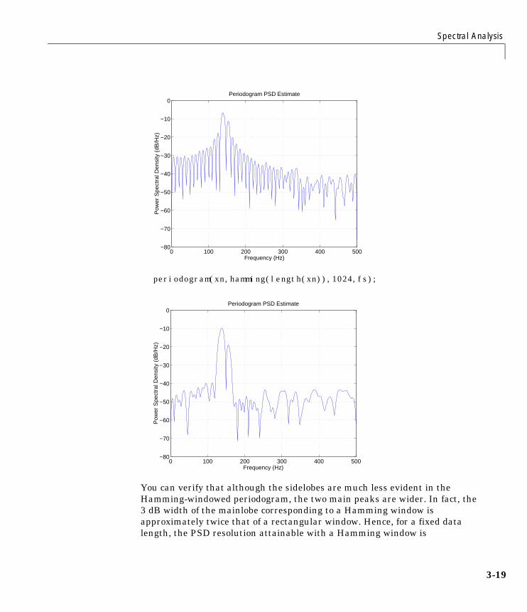
Spectral Analysis
3-19
periodogram(xn,hamming(length(xn)),1024,fs);
You can verify that although the sidelobes are much less evident in theHamming-windowed periodogram, the two main peaks are wider. In fact, the3 dB width of the mainlobe corresponding to a Hamming window isapproximately twice that of a rectangular window. Hence, for a fixed datalength, the PSD resolution attainable with a Hamming window is
0 100 200 300 400 500−80
−70
−60
−50
−40
−30
−20
−10
0
Frequency (Hz)
Pow
er S
pect
ral D
ensi
ty (
dB/H
z)
Periodogram PSD Estimate
0 100 200 300 400 500−80
−70
−60
−50
−40
−30
−20
−10
0
Frequency (Hz)
Pow
er S
pect
ral D
ensi
ty (
dB/H
z)
Periodogram PSD Estimate

3 Statistical Signal Processing
3-20
approximately half that attainable with a rectangular window. The competinginterests of mainlobe width and sidelobe height can be resolved to some extentby using variable windows such as the Kaiser window.
Nonrectangular windowing affects the average power of a signal because someof the time samples are attenuated when multiplied by the window. Tocompensate for this, the periodogram function normalizes the window to havean average power of unity. This way the choice of window does not affect theaverage power of the signal.
The modified periodogram estimate of the PSD is
where U is the window normalization constant
which is independent of the choice of window. The addition of U as anormalization constant ensures that the modified periodogram isasymptotically unbiased.
Welch’s MethodAn improved estimator of the PSD is the one proposed by Welch [8]. Themethod consists of dividing the time series data into (possibly overlapping)segments, computing a modified periodogram of each segment, and thenaveraging the PSD estimates. The result is Welch’s PSD estimate.
Welch’s method is implemented in the Signal Processing Toolbox by the pwelchfunction. By default, the data is divided into eight segments with 50% overlapbetween them. A Hamming window is used to compute the modifiedperiodogram of each segment.
The averaging of modified periodograms tends to decrease the variance of theestimate relative to a single periodogram estimate of the entire data record.Although overlap between segments tends to introduce redundant information,this effect is diminished by the use of a nonrectangular window, which reduces
Pxx f( )XL f( ) 2
fsLU--------------------=
U 1L---- w n( ) 2
n 0=
L 1–
=
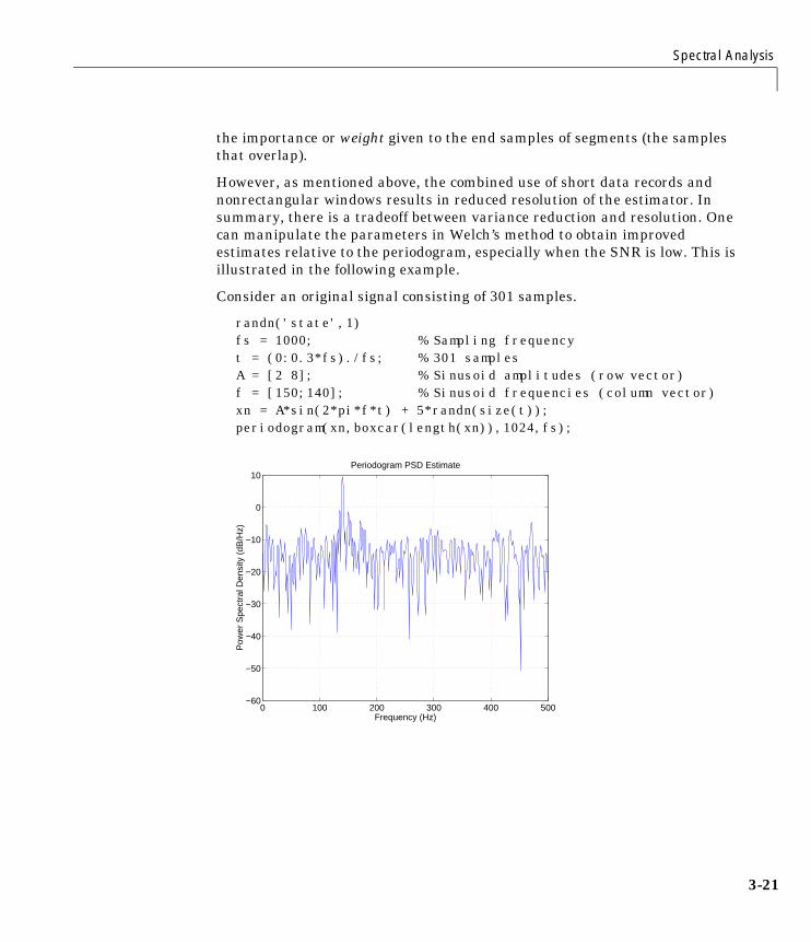
Spectral Analysis
3-21
the importance or weight given to the end samples of segments (the samplesthat overlap).
However, as mentioned above, the combined use of short data records andnonrectangular windows results in reduced resolution of the estimator. Insummary, there is a tradeoff between variance reduction and resolution. Onecan manipulate the parameters in Welch’s method to obtain improvedestimates relative to the periodogram, especially when the SNR is low. This isillustrated in the following example.
Consider an original signal consisting of 301 samples.
randn('state',1)fs = 1000; % Sampling frequencyt = (0:0.3*fs)./fs; % 301 samplesA = [2 8]; % Sinusoid amplitudes (row vector)f = [150;140]; % Sinusoid frequencies (column vector)xn = A*sin(2*pi*f*t) + 5*randn(size(t));periodogram(xn,boxcar(length(xn)),1024,fs);
0 100 200 300 400 500−60
−50
−40
−30
−20
−10
0
10
Frequency (Hz)
Pow
er S
pect
ral D
ensi
ty (
dB/H
z)
Periodogram PSD Estimate
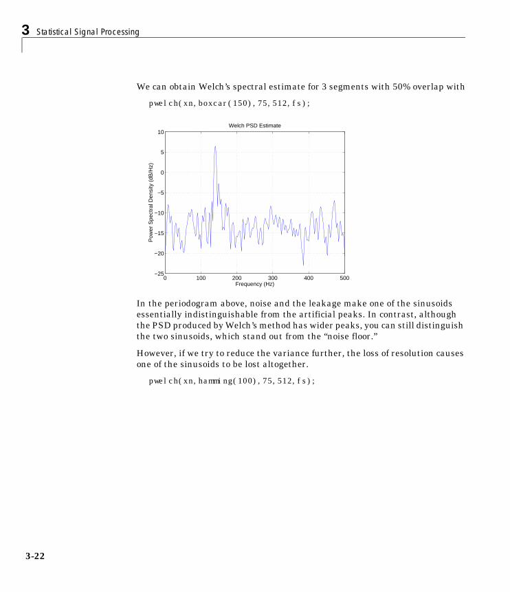
3 Statistical Signal Processing
3-22
We can obtain Welch’s spectral estimate for 3 segments with 50% overlap with
pwelch(xn,boxcar(150),75,512,fs);
In the periodogram above, noise and the leakage make one of the sinusoidsessentially indistinguishable from the artificial peaks. In contrast, althoughthe PSD produced by Welch’s method has wider peaks, you can still distinguishthe two sinusoids, which stand out from the “noise floor.”
However, if we try to reduce the variance further, the loss of resolution causesone of the sinusoids to be lost altogether.
pwelch(xn,hamming(100),75,512,fs);
0 100 200 300 400 500−25
−20
−15
−10
−5
0
5
10
Frequency (Hz)
Pow
er S
pect
ral D
ensi
ty (
dB/H
z)
Welch PSD Estimate
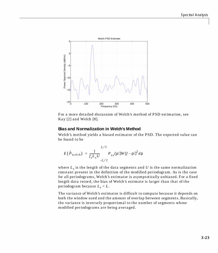
Spectral Analysis
3-23
For a more detailed discussion of Welch’s method of PSD estimation, seeKay [2] and Welch [8].
Bias and Normalization in Welch’s MethodWelch’s method yields a biased estimator of the PSD. The expected value canbe found to be
where Ls is the length of the data segments and U is the same normalizationconstant present in the definition of the modified periodogram. As is the casefor all periodograms, Welch’s estimator is asymptotically unbiased. For a fixedlength data record, the bias of Welch’s estimate is larger than that of theperiodogram because Ls < L.
The variance of Welch’s estimator is difficult to compute because it depends onboth the window used and the amount of overlap between segments. Basically,the variance is inversely proportional to the number of segments whosemodified periodograms are being averaged.
0 100 200 300 400 500−20
−15
−10
−5
0
5
Frequency (Hz)
Pow
er S
pect
ral D
ensi
ty (
dB/H
z)
Welch PSD Estimate
E Pwelch 1fsLsU---------------- Pxx ρ( ) W f ρ–( ) 2 ρd
fs 2⁄–
fs 2⁄
=

3 Statistical Signal Processing
3-24
Multitaper MethodThe periodogram can be interpreted as filtering a length L signal, xL[n],through a filter bank (a set of filters in parallel) of L FIR bandpass filters. The3 dB bandwidth of each of these bandpass filters can be shown to beapproximately equal to fs / L. The magnitude response of each one of thesebandpass filters resembles that of the rectangular window discussed in“Spectral Leakage” on page 3-12. The periodogram can thus be viewed as acomputation of the power of each filtered signal (i.e., the output of eachbandpass filter) that uses just one sample of each filtered signal and assumesthat the PSD of xL[n] is constant over the bandwidth of each bandpass filter.
As the length of the signal increases, the bandwidth of each bandpass filterdecreases, making it a more selective filter, and improving the approximationof constant PSD over the bandwidth of the filter. This provides anotherinterpretation of why the PSD estimate of the periodogram improves as thelength of the signal increases. However, there are two factors apparent fromthis standpoint that compromise the accuracy of the periodogram estimate.First, the rectangular window yields a poor bandpass filter. Second, thecomputation of the power at the output of each bandpass filter relies on a singlesample of the output signal, producing a very crude approximation.
Welch’s method can be given a similar interpretation in terms of a filter bank.In Welch’s implementation, several samples are used to compute the outputpower, resulting in reduced variance of the estimate. On the other hand, thebandwidth of each bandpass filter is larger than that corresponding to theperiodogram method, which results in a loss of resolution. The filter bankmodel thus provides a new interpretation of the compromise between varianceand resolution.
Thompson’s multitaper method (MTM) builds on these results to provide animproved PSD estimate. Instead of using bandpass filters that are essentiallyrectangular windows (as in the periodogram method), the MTM method uses abank of optimal bandpass filters to compute the estimate. These optimal FIRfilters are derived from a set of sequences known as discrete prolate spheroidalsequences (DPSSs, also known as Slepian sequences).
In addition, the MTM method provides a time-bandwidth parameter withwhich to balance the variance and resolution. This parameter is given by thetime-bandwidth product, NW and it is directly related to the number of tapersused to compute the spectrum. There are always 2*NW-1 tapers used to formthe estimate. This means that, as NW increases, there are more estimates of

Spectral Analysis
3-25
the power spectrum, and the variance of the estimate decreases. However, thebandwidth of each taper is also proportional to NW, so as NW increases, eachestimate exhibits more spectral leakage (i.e., wider peaks) and the overallspectral estimate is more biased. For each data set, there is usually a value forNW that allows an optimal trade-off between bias and variance.
The Signal Processing Toolbox function that implements the MTM method iscalled pmtm. Use pmtm to compute the PSD of xn from the previous examples.
randn('state',0)fs = 1000; % Sampling frequencyt = (0:fs)/fs; % One second worth of samplesA = [1 2]; % Sinusoid amplitudesf = [150;140]; % Sinusoid frequenciesxn = A*sin(2*pi*f*t) + 0.1*randn(size(t));
[P,F] = pmtm(xn,4,1024,fs);plot(F,10*log10(P)) % Plot in dB/Hzxlabel('Frequency (Hz)');ylabel('Power Spectral Density (dB/Hz)');
0 100 200 300 400 500−55
−50
−45
−40
−35
−30
−25
−20
−15
−10
−5
Frequency (Hz)
Pow
er S
pect
ral D
ensi
ty (
dB/H
z)

3 Statistical Signal Processing
3-26
By lowering the time-bandwidth product, you can increase the resolution at theexpense of larger variance.
[P1,f] = pmtm(xn,3/2,1024,fs);plot(f,10*log10(P1)) % Plot in dB/Hzxlabel('Frequency (Hz)');ylabel('Power Spectral Density (dB/Hz)');
Note that the average power is conserved in both cases.
Pow = (fs/1024) * sum(P)
Pow =
2.4926
Pow1 = (fs/1024) * sum(P1)
Pow1 =
2.4927
This method is more computationally expensive than Welch’s method due tothe cost of computing the discrete prolate spheroidal sequences. For long dataseries (10,000 points or more), it is useful to compute the DPSSs once and savethem in a MAT-file. The M-files dpsssave, dpssload, dpssdir, and dpssclearare provided to keep a database of saved DPSSs in the MAT-file dpss.mat.
0 100 200 300 400 500−80
−70
−60
−50
−40
−30
−20
−10
0
Frequency (Hz)
Pow
er S
pect
ral D
ensi
ty (
dB/H
z)
Spectral Analysis
3-27
Cross-Spectral Density FunctionThe PSD is a special case of the cross spectral density (CSD) function, definedbetween two signals xn and yn as
As is the case for the correlation and covariance sequences, the toolboxestimates the PSD and CSD because signal lengths are finite.
To estimate the cross-spectral density of two equal length signals x and y usingWelch’s method, the csd function forms the periodogram as the product of theFFT of x and the conjugate of the FFT of y. Unlike the real-valued PSD, theCSD is a complex function. csd handles the sectioning and windowing of x andy in the same way as the pwelch function.
Sxy = csd(x,y,nfft,fs,window,numoverlap)
Confidence IntervalsYou can compute confidence intervals using the csd function by including anadditional input argument p that specifies the percentage of the confidenceinterval, and setting the numoverlap argument to 0.
[Sxy,Sxyc,f] = csd(x,y,nfft,fs,window,0,p)
p must be a scalar between 0 and 1. This function assumes chi-squareddistributed periodograms of the nonoverlapping sections of windowed data incomputing the confidence intervals. This assumption is valid when the signalis a Gaussian distributed random process. Provided these assumptions arecorrect, the confidence interval
[Sxy-Sxyc(:,1) Sxy+Sxyc(:,2)]
covers the true CSD with probability p. If you set numoverlap to any valueother than 0, you generate a warning indicating that the sections overlap andthe confidence interval is not reliable.
Sxy ω( ) Rxy m( )e jωm–
m ∞–=
∞
=
3 Statistical Signal Processing
3-28
Transfer Function EstimateOne application of Welch’s method is nonparametric system identification.Assume that H is a linear, time invariant system, and x(n) and y(n) are theinput to and output of H, respectively. Then the power spectrum of x(n) isrelated to the CSD of x(n) and y(n) by
An estimate of the transfer function between x(n) and y(n) is
This method estimates both magnitude and phase information. The tfefunction uses Welch’s method to compute the CSD and power spectrum, andthen forms their quotient for the transfer function estimate. Use tfe the sameway that you use the csd function.
Filter the signal xn with an FIR filter, then plot the actual magnitude responseand the estimated response.
h = ones(1,10)/10; % Moving average filteryn = filter(h,1,xn);[HEST,f] = tfe(xn,yn,256,fs,256,128,'none');H = freqz(h,1,f,fs);
subplot(2,1,1); plot(f,abs(H)); title('Actual Transfer Function Magnitude');
subplot(2,1,2); plot(f,abs(HEST));title('Transfer Function Magnitude Estimate'); xlabel('Frequency (Hz)');
Sxy ω( ) H ω( )Sxx ω( )=
H ω( )Sxy ω( )
Sxx ω( )-----------------=
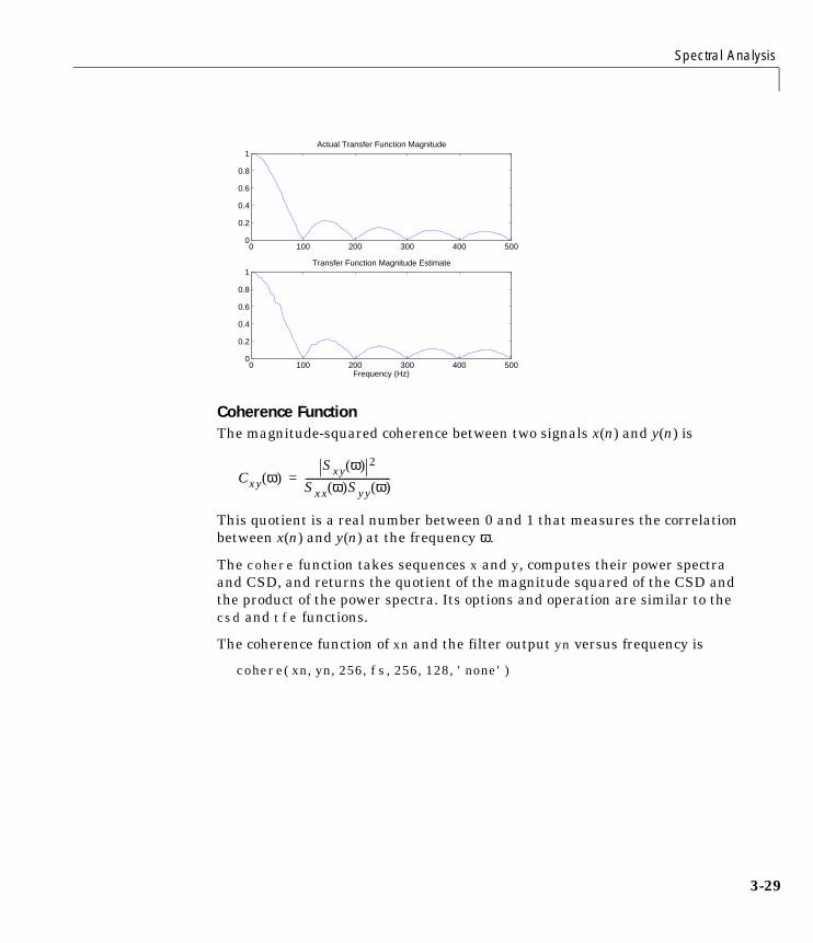
Spectral Analysis
3-29
Coherence FunctionThe magnitude-squared coherence between two signals x(n) and y(n) is
This quotient is a real number between 0 and 1 that measures the correlationbetween x(n) and y(n) at the frequency ω.
The cohere function takes sequences x and y, computes their power spectraand CSD, and returns the quotient of the magnitude squared of the CSD andthe product of the power spectra. Its options and operation are similar to thecsd and tfe functions.
The coherence function of xn and the filter output yn versus frequency is
cohere(xn,yn,256,fs,256,128,'none')
0 100 200 300 400 5000
0.2
0.4
0.6
0.8
1Actual Transfer Function Magnitude
0 100 200 300 400 5000
0.2
0.4
0.6
0.8
1Transfer Function Magnitude Estimate
Frequency (Hz)
Cxy ω( )Sxy ω( ) 2
Sxx ω( )Syy ω( )-----------------------------------=

3 Statistical Signal Processing
3-30
If the input sequence length nfft, window length window, and the number ofoverlapping data points in a window numoverlap, are such that cohereoperates on only a single record, the function returns all ones. This is becausethe coherence function for linearly dependent data is one.
Parametric MethodsParametric methods can yield higher resolutions than nonparametric methodsin cases when the signal length is short. These methods use a differentapproach to spectral estimation; instead of trying to estimate the PSD directlyfrom the data, they model the data as the output of a linear system driven bywhite noise, and then attempt to estimate the parameters of that linearsystem.
The most commonly used linear system model is the all-pole model, a filterwith all of its zeroes at the origin in the z-plane. The output of such a filter forwhite noise input is an autoregressive (AR) process. For this reason, thesemethods are sometimes referred to as AR methods of spectral estimation.
The AR methods tend to adequately describe spectra of data that is “peaky,”that is, data whose PSD is large at certain frequencies. The data in manypractical applications (such as speech) tends to have “peaky spectra” so that ARmodels are often useful. In addition, the AR models lead to a system of linearequations which is relatively simple to solve.
The Signal Processing Toolbox offers the following AR methods for spectralestimation:
• Yule-Walker AR method (autocorrelation method)
• Burg method
0 50 100 150 200 250 300 350 400 450 5000
0.2
0.4
0.6
0.8
1
Frequency
Coh
eren
ce F
unct
ion
Est
imat
e
Coherence Function

Spectral Analysis
3-31
• Covariance method
• Modified covariance method
All AR methods yield a PSD estimate given by
The different AR methods estimate the AR parameters ap(k) slightlydifferently, yielding different PSD estimates. The following table provides asummary of the different AR methods.
PAR f( ) 1fs----
εp
1 ap k( )e2πjkf– fs⁄
k 1=
p
+
2-------------------------------------------------------------------=
Burg Covariance Modified Covariance Yule-Walker
Characteristics Does not applywindow to data
Does not applywindow to data
Does not applywindow to data
Applies window todata
Minimizes theforward and backwardprediction errors inthe least squaressense, with the ARcoefficientsconstrained to satisfythe L-D recursion
Minimizes theforward predictionerror in the leastsquares sense
Minimizes theforward and backwardprediction errors inthe least squaressense
Minimizes theforward predictionerror in the leastsquares sense(also called“Autocorrelationmethod”)
Advantages High resolution forshort data records
Better resolution thanY-W for short datarecords (moreaccurate estimates)
High resolution forshort data records
Performs as well asother methods forlarge data records
Always produces astable model
Able to extractfrequencies from dataconsisting of p or morepure sinusoids
Able to extractfrequencies from dataconsisting of p or morepure sinusoids
Always produces astable model
Does not sufferspectral line-splitting
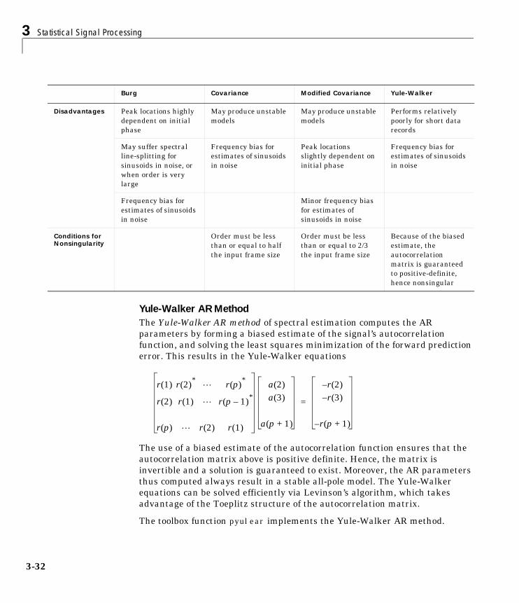
3 Statistical Signal Processing
3-32
Yule-Walker AR MethodThe Yule-Walker AR method of spectral estimation computes the ARparameters by forming a biased estimate of the signal’s autocorrelationfunction, and solving the least squares minimization of the forward predictionerror. This results in the Yule-Walker equations
The use of a biased estimate of the autocorrelation function ensures that theautocorrelation matrix above is positive definite. Hence, the matrix isinvertible and a solution is guaranteed to exist. Moreover, the AR parametersthus computed always result in a stable all-pole model. The Yule-Walkerequations can be solved efficiently via Levinson’s algorithm, which takesadvantage of the Toeplitz structure of the autocorrelation matrix.
The toolbox function pyulear implements the Yule-Walker AR method.
Disadvantages Peak locations highlydependent on initialphase
May produce unstablemodels
May produce unstablemodels
Performs relativelypoorly for short datarecords
May suffer spectralline-splitting forsinusoids in noise, orwhen order is verylarge
Frequency bias forestimates of sinusoidsin noise
Peak locationsslightly dependent oninitial phase
Frequency bias forestimates of sinusoidsin noise
Frequency bias forestimates of sinusoidsin noise
Minor frequency biasfor estimates ofsinusoids in noise
Conditions for Nonsingularity
Order must be lessthan or equal to halfthe input frame size
Order must be lessthan or equal to 2/3the input frame size
Because of the biasedestimate, theautocorrelationmatrix is guaranteedto positive-definite,hence nonsingular
Burg Covariance Modified Covariance Yule-Walker
r 1( ) r 2( )*
r p( )*
r 2( ) r 1( ) r p 1–( )*
r p( ) r 2( ) r 1( )
a 2( )
a 3( )
a p 1+( )
r 2( )–
r 3( )–
r p 1+( )–
=

Spectral Analysis
3-33
For example, compare the spectrum of a speech signal using Welch’s methodand the Yule-Walker AR method.
load mtlb[P1,f] = pwelch(mtlb,hamming(256),128,1024,fs);[P2,f] = pyulear(mtlb,14,1024,fs);plot(f,10*log10(P1),':',f,10*log10(P2)); gridylabel('PSD Estimates (dB/Hz)');xlabel('Frequency (Hz)');legend('Welch','Yule-Walker AR')
The solid-line Yule-Walker AR spectrum is smoother than the periodogrambecause of the simple underlying all-pole model.
Burg MethodThe Burg method for AR spectral estimation is based on minimizing theforward and backward prediction errors while satisfying the Levinson-Durbinrecursion (see Marple [3], Chapter 7, and Proakis [6], Section 12.3.3). Incontrast to other AR estimation methods, the Burg method avoids calculatingthe autocorrelation function, and instead estimates the reflection coefficientsdirectly.
The primary advantages of the Burg method are resolving closely spacedsinusoids in signals with low noise levels, and estimating short data records, in
0 100 200 300 400 500 600−70
−60
−50
−40
−30
−20
−10
PS
D E
stim
ates
(dB
/Hz)
Frequency (Hz)
WelchYule−Walker AR

3 Statistical Signal Processing
3-34
which case the AR power spectral density estimates are very close to the truevalues. In addition, the Burg method ensures a stable AR model and iscomputationally efficient.
The accuracy of the Burg method is lower for high-order models, long datarecords, and high signal-to-noise ratios (which can cause line splitting, or thegeneration of extraneous peaks in the spectrum estimate). The spectral densityestimate computed by the Burg method is also susceptible to frequency shifts(relative to the true frequency) resulting from the initial phase of noisysinusoidal signals. This effect is magnified when analyzing short datasequences.
The toolbox function pburg implements the Burg method. Compare thespectrum of the speech signal generated by both the Burg method and theYule-Walker AR method. They are very similar for large signal lengths.
load mtlb[P1,f] = pburg(mtlb(1:512),14,1024,fs); % 14th order model[P2,f] = pyulear(mtlb(1:512),14,1024,fs); % 14th order modelplot(f,10*log10(P1),':',f,10*log10(P2)); gridylabel('Magnitude (dB)'); xlabel('Frequency (Hz)');legend('Burg','Yule-Walker AR')
0 100 200 300 400 500 600−80
−70
−60
−50
−40
−30
−20
−10
Mag
nitu
de (
dB)
Frequency (Hz)
BurgYule−Walker AR

Spectral Analysis
3-35
Compare the spectrum of a noisy signal computed using the Burg method andthe Welch method.
randn('state',0)fs = 1000; % Sampling frequencyt = (0:fs)/fs; % One second worth of samplesA = [1 2]; % Sinusoid amplitudesf = [150;140]; % Sinusoid frequenciesxn = A*sin(2*pi*f*t) + 0.1*randn(size(t));
[P1,f] = pwelch(xn,hamming(256),128,1024,fs);[P2,f] = pburg(xn,14,1024,fs);
plot(f,10*log10(P1),':',f,10*log10(P2)); gridylabel('PSD Estimates (dB/Hz)');xlabel('Frequency (Hz)');legend('Welch','Burg')
Note that, as the model order for the Burg method is reduced, a frequency shiftdue to the initial phase of the sinusoids will become apparent.
0 100 200 300 400 500 600−60
−50
−40
−30
−20
−10
0
PS
D E
stim
ates
(dB
/Hz)
Frequency (Hz)
WelchBurg
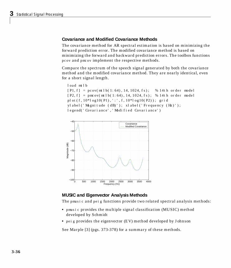
3 Statistical Signal Processing
3-36
Covariance and Modified Covariance MethodsThe covariance method for AR spectral estimation is based on minimizing theforward prediction error. The modified covariance method is based onminimizing the forward and backward prediction errors. The toolbox functionspcov and pmcov implement the respective methods.
Compare the spectrum of the speech signal generated by both the covariancemethod and the modified covariance method. They are nearly identical, evenfor a short signal length.
load mtlb[P1,f] = pcov(mtlb(1:64),14,1024,fs); % 14th order model[P2,f] = pmcov(mtlb(1:64),14,1024,fs); % 14th order modelplot(f,10*log10(P1),':',f,10*log10(P2)); gridylabel('Magnitude (dB)'); xlabel('Frequency (Hz)');legend('Covariance','Modified Covariance')
MUSIC and Eigenvector Analysis MethodsThe pmusic and peig functions provide two related spectral analysis methods:
• pmusic provides the multiple signal classification (MUSIC) methoddeveloped by Schmidt
• peig provides the eigenvector (EV) method developed by Johnson
See Marple [3] (pgs. 373-378) for a summary of these methods.
0 500 1000 1500 2000 2500 3000 3500 4000−100
−90
−80
−70
−60
−50
−40
Mag
nitu
de (
dB)
Frequency (Hz)
Covariance Modified Covariance
Spectral Analysis
3-37
Both of these methods are frequency estimator techniques based oneigenanalysis of the autocorrelation matrix. This type of spectral analysiscategorizes the information in a correlation or data matrix, assigninginformation to either a signal subspace or a noise subspace.
Eigenanalysis OverviewConsider a number of complex sinusoids embedded in white noise. You canwrite the autocorrelation matrix R for this system as the sum of the signalautocorrelation matrix (S) and the noise autocorrelation matrix (W).
There is a close relationship between the eigenvectors of the signalautocorrelation matrix and the signal and noise subspaces. The eigenvectors vof S span the same signal subspace as the signal vectors. If the system containsM complex sinusoids and the order of the autocorrelation matrix is p,eigenvectors vM+1 through vp+1 span the noise subspace of the autocorrelationmatrix.
Frequency Estimator Functions. To generate their frequency estimates,eigenanalysis methods calculate functions of the vectors in the signal and noisesubspaces. Both the MUSIC and EV techniques choose a function that goes toinfinity (denominator goes to zero) at one of the sinusoidal frequencies in theinput signal. Using digital technology, the resulting estimate has sharp peaksat the frequencies of interest; this means that there might not be infinityvalues in the vectors.
The MUSIC estimate is given by the formula
where N is the size of the eigenvectors and e(f) is a vector of complex sinusoids.
v represents the eigenvectors of the input signal’s correlation matrix; vk is thekth eigenvector. H is the conjugate transpose operator. The eigenvectors used
R S W+=
Pmusicf( )1
eH f( ) vkvkH
k p 1+=
N
e f( )
----------------------------------------------------------------1
vkHe f( ) 2
k p 1+=
N
-------------------------------------------= =
e f( ) 1 exp j2πf( ) exp j2πf 2⋅( ) exp j2πf 4⋅( ) … exp j2πf n 1–( )⋅( )[ ]H=
3 Statistical Signal Processing
3-38
in the sum correspond to the smallest eigenvalues and span the noise subspace(p is the size of the signal subspace).
The expression is equivalent to a Fourier transform (the vector e(f)consists of complex exponentials). This form is useful for numeric computationbecause the FFT can be computed for each vk and then the squared magnitudescan be summed.
The EV method weights the summation by the eigenvalues of the correlationmatrix.
The pmusic and peig functions in this toolbox use the svd (singular valuedecomposition) function in the signal case and the eig function for analyzingthe correlation matrix and assigning eigenvectors to the signal or noisesubspaces. When svd is used, pmusic and peig never compute the correlationmatrix explicitly, but the singular values are the eigenvalues.
vkHe f( )
Pev f( )1
vkHe f( ) 2
k p 1+=
N
λk⁄
-----------------------------------------------------------=

Selected Bibliography
3-39
Selected Bibliography[1] Hayes, M.H. Statistical Digital Signal Processing and Modeling. New York:John Wiley & Sons, 1996.
[2] Kay, S.M. Modern Spectral Estimation. Englewood Cliffs, NJ: Prentice Hall,1988.
[3] Marple, S.L. Digital Spectral Analysis. Englewood Cliffs, NJ: Prentice Hall,1987.
[4] Orfanidis, S.J. Introduction to Signal Processing. Upper Saddle River, NJ:Prentice Hall, 1996.
[5] Percival, D.B., and A.T. Walden. Spectral Analysis for PhysicalApplications: Multitaper and Conventional Univariate Techniques. Cambridge:Cambridge University Press, 1993.
[6] Proakis, J.G., and D.G. Manolakis. Digital Signal Processing: Principles,Algorithms, and Applications. Englewood Cliffs, NJ: Prentice Hall, 1996.
[7] Stoica, P., and R. Moses. Introduction to Spectral Analysis. Upper SaddleRiver, NJ: Prentice Hall, 1997.
[8] Welch, P.D. “The Use of Fast Fourier Transform for the Estimation of PowerSpectra: A Method Based on Time Averaging Over Short, ModifiedPeriodograms.” IEEE Trans. Audio Electroacoust. Vol. AU-15 (June 1967).Pgs. 70-73.

3 Statistical Signal Processing
3-40
4
Special Topics
Overview . . . . . . . . . . . . . . . . . . . . . 4-2
Windows . . . . . . . . . . . . . . . . . . . . . . 4-3Basic Shapes . . . . . . . . . . . . . . . . . . . . 4-3Generalized Cosine Windows . . . . . . . . . . . . . . 4-5Kaiser Window . . . . . . . . . . . . . . . . . . . 4-5Chebyshev Window . . . . . . . . . . . . . . . . . . 4-9
Parametric Modeling . . . . . . . . . . . . . . . . 4-11Time-Domain Based Modeling . . . . . . . . . . . . . 4-13Frequency-Domain Based Modeling . . . . . . . . . . . 4-18
Resampling . . . . . . . . . . . . . . . . . . . . 4-21
Cepstrum Analysis . . . . . . . . . . . . . . . . . 4-24Inverse Complex Cepstrum . . . . . . . . . . . . . . 4-26
FFT-Based Time-Frequency Analysis . . . . . . . . . 4-28
Median Filtering . . . . . . . . . . . . . . . . . . 4-29
Communications Applications . . . . . . . . . . . . 4-30
Deconvolution . . . . . . . . . . . . . . . . . . . 4-34
Specialized Transforms . . . . . . . . . . . . . . . 4-35Chirp z-Transform . . . . . . . . . . . . . . . . . . 4-35Discrete Cosine Transform . . . . . . . . . . . . . . . 4-37Hilbert Transform . . . . . . . . . . . . . . . . . . 4-39
Selected Bibliography . . . . . . . . . . . . . . . 4-41

4 Special Topics
4-2
OverviewThe Signal Processing Toolbox provides functions that allow you to apply avariety of signal processing techniques. The following sections describe how touse some of these functions:
• “Windows”
• “Parametric Modeling”
• “Resampling”
• “Cepstrum Analysis”
• “FFT-Based Time-Frequency Analysis”
• “Median Filtering”
• “Communications Applications”
• “Deconvolution”
• “Specialized Transforms”
• “Selected Bibliography”
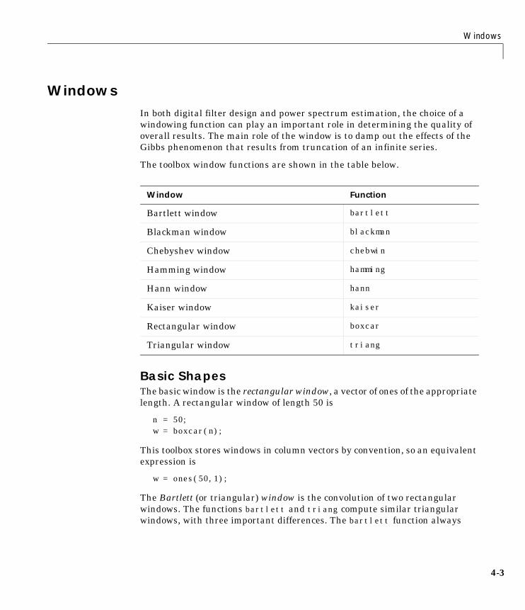
Windows
4-3
WindowsIn both digital filter design and power spectrum estimation, the choice of awindowing function can play an important role in determining the quality ofoverall results. The main role of the window is to damp out the effects of theGibbs phenomenon that results from truncation of an infinite series.
The toolbox window functions are shown in the table below.
Basic ShapesThe basic window is the rectangular window, a vector of ones of the appropriatelength. A rectangular window of length 50 is
n = 50;w = boxcar(n);
This toolbox stores windows in column vectors by convention, so an equivalentexpression is
w = ones(50,1);
The Bartlett (or triangular) window is the convolution of two rectangularwindows. The functions bartlett and triang compute similar triangularwindows, with three important differences. The bartlett function always
Window Function
Bartlett window bartlett
Blackman window blackman
Chebyshev window chebwin
Hamming window hamming
Hann window hann
Kaiser window kaiser
Rectangular window boxcar
Triangular window triang
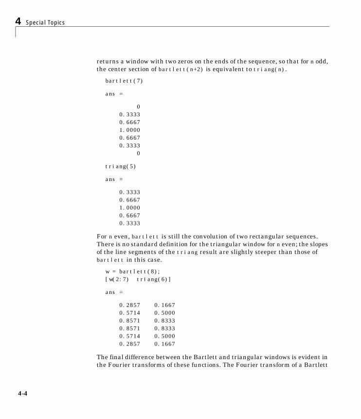
4 Special Topics
4-4
returns a window with two zeros on the ends of the sequence, so that for n odd,the center section of bartlett(n+2) is equivalent to triang(n).
bartlett(7)
ans =
0 0.3333 0.6667 1.0000 0.6667 0.3333 0
triang(5)
ans =
0.3333 0.6667 1.0000 0.6667 0.3333
For n even, bartlett is still the convolution of two rectangular sequences.There is no standard definition for the triangular window for n even; the slopesof the line segments of the triang result are slightly steeper than those ofbartlett in this case.
w = bartlett(8); [w(2:7) triang(6)]
ans =
0.2857 0.1667 0.5714 0.5000 0.8571 0.8333 0.8571 0.8333 0.5714 0.5000 0.2857 0.1667
The final difference between the Bartlett and triangular windows is evident inthe Fourier transforms of these functions. The Fourier transform of a Bartlett
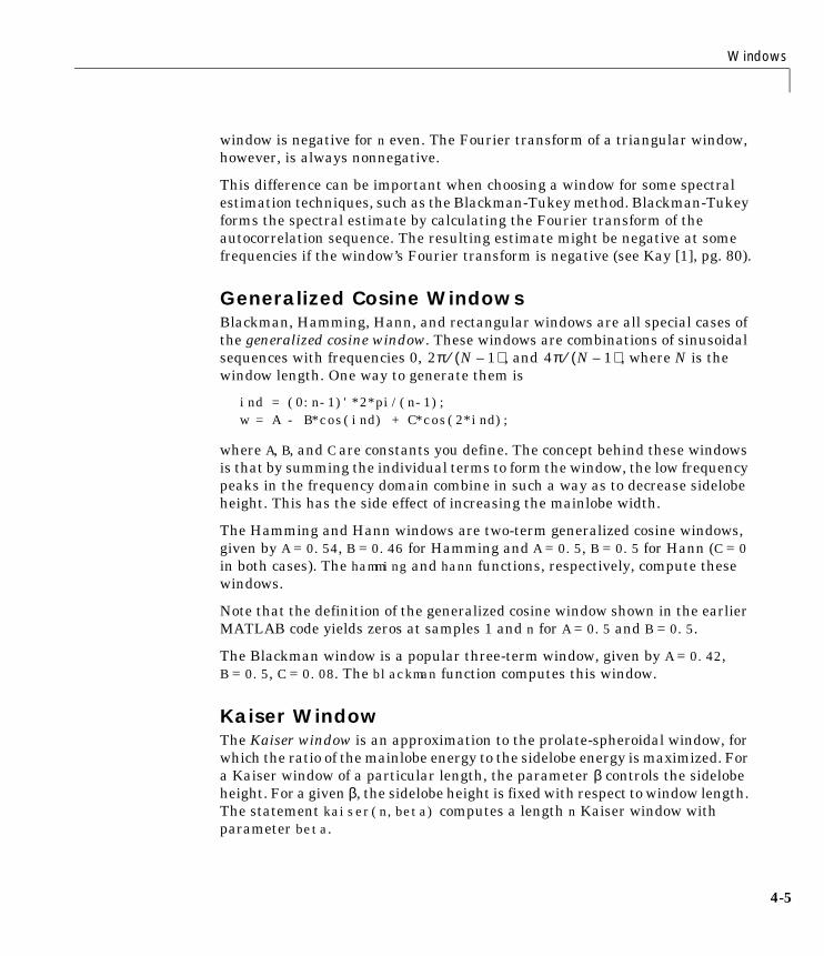
Windows
4-5
window is negative for n even. The Fourier transform of a triangular window,however, is always nonnegative.
This difference can be important when choosing a window for some spectralestimation techniques, such as the Blackman-Tukey method. Blackman-Tukeyforms the spectral estimate by calculating the Fourier transform of theautocorrelation sequence. The resulting estimate might be negative at somefrequencies if the window’s Fourier transform is negative (see Kay [1], pg. 80).
Generalized Cosine WindowsBlackman, Hamming, Hann, and rectangular windows are all special cases ofthe generalized cosine window. These windows are combinations of sinusoidalsequences with frequencies 0, , and , where N is thewindow length. One way to generate them is
ind = (0:n-1)'*2*pi/(n-1);w = A - B*cos(ind) + C*cos(2*ind);
where A, B, and C are constants you define. The concept behind these windowsis that by summing the individual terms to form the window, the low frequencypeaks in the frequency domain combine in such a way as to decrease sidelobeheight. This has the side effect of increasing the mainlobe width.
The Hamming and Hann windows are two-term generalized cosine windows,given by A = 0.54, B = 0.46 for Hamming and A = 0.5, B = 0.5 for Hann (C = 0in both cases). The hamming and hann functions, respectively, compute thesewindows.
Note that the definition of the generalized cosine window shown in the earlierMATLAB code yields zeros at samples 1 and n for A = 0.5 and B = 0.5.
The Blackman window is a popular three-term window, given by A = 0.42,B = 0.5, C = 0.08. The blackman function computes this window.
Kaiser WindowThe Kaiser window is an approximation to the prolate-spheroidal window, forwhich the ratio of the mainlobe energy to the sidelobe energy is maximized. Fora Kaiser window of a particular length, the parameter β controls the sidelobeheight. For a given β, the sidelobe height is fixed with respect to window length.The statement kaiser(n,beta) computes a length n Kaiser window withparameter beta.
2π N 1–( )⁄ 4π N 1–( )⁄
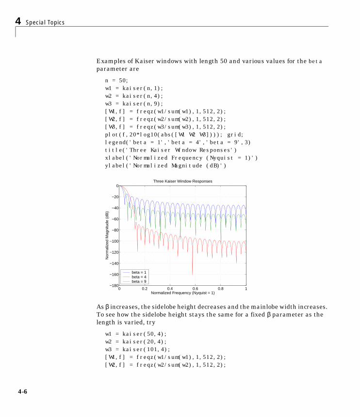
4 Special Topics
4-6
Examples of Kaiser windows with length 50 and various values for the betaparameter are
n = 50;w1 = kaiser(n,1);w2 = kaiser(n,4);w3 = kaiser(n,9);[W1,f] = freqz(w1/sum(w1),1,512,2);[W2,f] = freqz(w2/sum(w2),1,512,2);[W3,f] = freqz(w3/sum(w3),1,512,2);plot(f,20*log10(abs([W1 W2 W3]))); grid;legend('beta = 1','beta = 4','beta = 9',3)title('Three Kaiser Window Responses')xlabel('Normalized Frequency (Nyquist = 1)')ylabel('Normalized Magnitude (dB)')
As β increases, the sidelobe height decreases and the mainlobe width increases.To see how the sidelobe height stays the same for a fixed β parameter as thelength is varied, try
w1 = kaiser(50,4);w2 = kaiser(20,4);w3 = kaiser(101,4);[W1,f] = freqz(w1/sum(w1),1,512,2);[W2,f] = freqz(w2/sum(w2),1,512,2);
0 0.2 0.4 0.6 0.8 1−180
−160
−140
−120
−100
−80
−60
−40
−20
0Three Kaiser Window Responses
Normalized Frequency (Nyquist = 1)
Nor
mal
ized
Mag
nitu
de (
dB)
beta = 1beta = 4beta = 9

Windows
4-7
[W3,f] = freqz(w3/sum(w3),1,512,2);plot(f,20*log10(abs([W1 W2 W3]))); grid;legend('length = 50','length = 20','length = 101')title('Three Kaiser Window Responses, Beta Fixed')xlabel('Normalized Frequency (Nyquist = 1)')ylabel('Normalized Magnitude (dB)')
Kaiser Windows in FIR DesignThere are two design formulas that can help you design FIR filters to meet aset of filter specifications using a Kaiser window. To achieve a sidelobe heightof −α dB, the beta parameter is
For a transition width of ∆ω rad/s, use the length
Filters designed using these heuristics will meet the specificationsapproximately, but you should verify this. To design a lowpass filter with cutoff
0 0.2 0.4 0.6 0.8 1−120
−100
−80
−60
−40
−20
0
20Three Kaiser Window Responses, Beta Fixed
Normalized Frequency (Nyquist = 1)
Nor
mal
ized
Mag
nitu
de (
dB)
length = 50length = 20length = 101
β0.1102 α 8.7–( ), α 50>0.5842 α 21–( )0.4 0.07886 α 21–( )+ , 50 α 21≥ ≥0, α 21<
=
n α 8–2.285 ω∆----------------------- 1+=

4 Special Topics
4-8
frequency rad/s, transition width rad/s, and 40 dB of attenuation inthe stopband, try
[n,wn,beta] = kaiserord([0.4 0.6]*pi,[1 0],[0.01 0.01],2*pi);h = fir1(n,wn,kaiser(n+1,beta),'noscale');
The kaiserord function estimates the filter order, cutoff frequency, and Kaiserwindow beta parameter needed to meet a given set of frequency domainspecifications.
The ripple in the passband is roughly the same as the ripple in the stopband.As you can see from the frequency response, this filter nearly meets thespecifications.
[H,f] = freqz(h,1,512,2);plot(f,20*log10(abs(H))), grid
For details on kaiserord, see the description in Chapter 7, “FunctionReference.”
0.5π 0.2π
0 0.1 0.2 0.3 0.4 0.5 0.6 0.7 0.8 0.9 1-100
-80
-60
-40
-20
0
20
Normalized Frequency (Nyquist == 1)
Mag
nitu
de (
dB)
FIR Design using Kaiser Window
0.2 40 dB
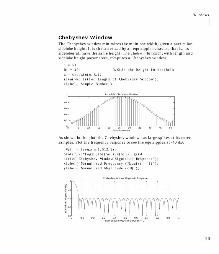
Windows
4-9
Chebyshev WindowThe Chebyshev window minimizes the mainlobe width, given a particularsidelobe height. It is characterized by an equiripple behavior, that is, itssidelobes all have the same height. The chebwin function, with length andsidelobe height parameters, computes a Chebyshev window.
n = 51;Rs = 40; % Sidelobe height in decibelsw = chebwin(n,Rs);stem(w); title('Length 51 Chebyshev Window');xlabel('Sample Number');
As shown in the plot, the Chebyshev window has large spikes at its outersamples. Plot the frequency response to see the equiripples at -40 dB.
[W,f] = freqz(w,1,512,2);plot(f,20*log10(abs(W)/sum(w))), gridtitle('Chebyshev Window Magnitude Response');xlabel('Normalized Frequency (Nyquist = 1)');ylabel('Normalized Magnitude (dB)');
0 5 10 15 20 25 30 35 40 45 500
0.2
0.4
0.6
0.8
1
Sample Number
Length 51 Chebyshev Window
0 0.1 0.2 0.3 0.4 0.5 0.6 0.7 0.8 0.9 1-80
-60
-40
-20
0
Normalized Frequency (Nyquist == 1)
Nor
mai
lzed
Mag
nitu
de (
dB)
Chebyshev Window Magnitude Response

4 Special Topics
4-10
For a detailed discussion of the characteristics and applications of the variouswindow types, see Oppenheim and Schafer [2], pgs. 444-462, and Parks andBurrus [3], pgs. 71-73.
Parametric Modeling
4-11
Parametric ModelingParametric modeling techniques find the parameters for a mathematical modeldescribing a signal, system, or process. These techniques use knowninformation about the system to determine the model. Applications forparametric modeling include speech and music synthesis, data compression,high-resolution spectral estimation, communications, manufacturing, andsimulation.
The toolbox parametric modeling functions operate with the rational transferfunction model. Given appropriate information about an unknown system(impulse or frequency response data, or input and output sequences), thesefunctions find the coefficients of a linear system that models the system.
One important application of the parametric modeling functions is in thedesign of filters that have a prescribed time or frequency response. Thesefunctions provide a data-oriented alternative to the IIR and FIR filter designfunctions discussed in Chapter 2, “Filter Design.”
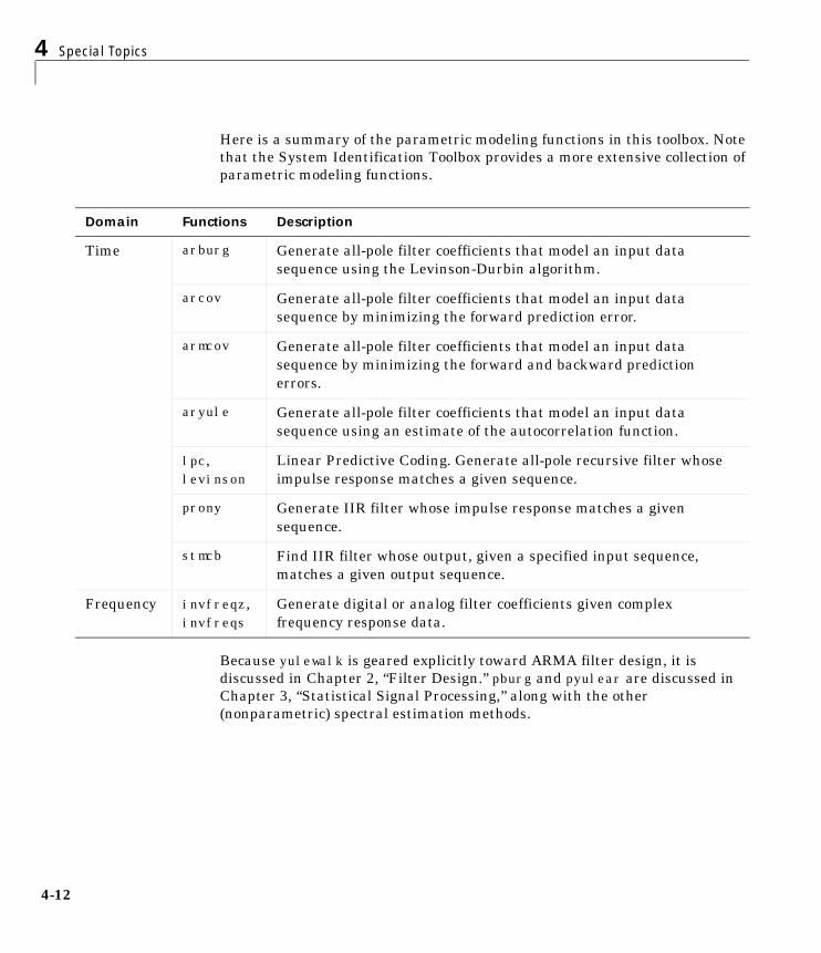
4 Special Topics
4-12
Here is a summary of the parametric modeling functions in this toolbox. Notethat the System Identification Toolbox provides a more extensive collection ofparametric modeling functions.
Because yulewalk is geared explicitly toward ARMA filter design, it isdiscussed in Chapter 2, “Filter Design.” pburg and pyulear are discussed inChapter 3, “Statistical Signal Processing,” along with the other(nonparametric) spectral estimation methods.
Domain Functions Description
Time arburg Generate all-pole filter coefficients that model an input datasequence using the Levinson-Durbin algorithm.
arcov Generate all-pole filter coefficients that model an input datasequence by minimizing the forward prediction error.
armcov Generate all-pole filter coefficients that model an input datasequence by minimizing the forward and backward predictionerrors.
aryule Generate all-pole filter coefficients that model an input datasequence using an estimate of the autocorrelation function.
lpc,levinson
Linear Predictive Coding. Generate all-pole recursive filter whoseimpulse response matches a given sequence.
prony Generate IIR filter whose impulse response matches a givensequence.
stmcb Find IIR filter whose output, given a specified input sequence,matches a given output sequence.
Frequency invfreqz,invfreqs
Generate digital or analog filter coefficients given complexfrequency response data.
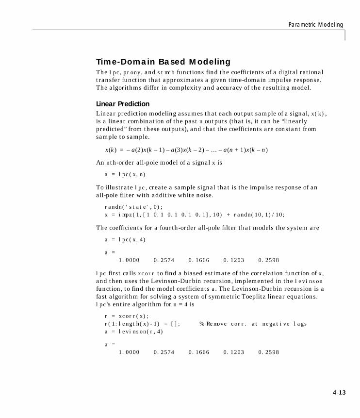
Parametric Modeling
4-13
Time-Domain Based ModelingThe lpc, prony, and stmcb functions find the coefficients of a digital rationaltransfer function that approximates a given time-domain impulse response.The algorithms differ in complexity and accuracy of the resulting model.
Linear PredictionLinear prediction modeling assumes that each output sample of a signal, x(k),is a linear combination of the past n outputs (that is, it can be “linearlypredicted” from these outputs), and that the coefficients are constant fromsample to sample.
An nth-order all-pole model of a signal x is
a = lpc(x,n)
To illustrate lpc, create a sample signal that is the impulse response of anall-pole filter with additive white noise.
randn('state',0);x = impz(1,[1 0.1 0.1 0.1 0.1],10) + randn(10,1)/10;
The coefficients for a fourth-order all-pole filter that models the system are
a = lpc(x,4)
a = 1.0000 0.2574 0.1666 0.1203 0.2598
lpc first calls xcorr to find a biased estimate of the correlation function of x,and then uses the Levinson-Durbin recursion, implemented in the levinsonfunction, to find the model coefficients a. The Levinson-Durbin recursion is afast algorithm for solving a system of symmetric Toeplitz linear equations.lpc’s entire algorithm for n = 4 is
r = xcorr(x);r(1:length(x)-1) = []; % Remove corr. at negative lagsa = levinson(r,4)
a = 1.0000 0.2574 0.1666 0.1203 0.2598
x k( ) a 2( )x k 1–( )– a 3( )x k 2–( )– …– a n 1+( )x k n–( )–=
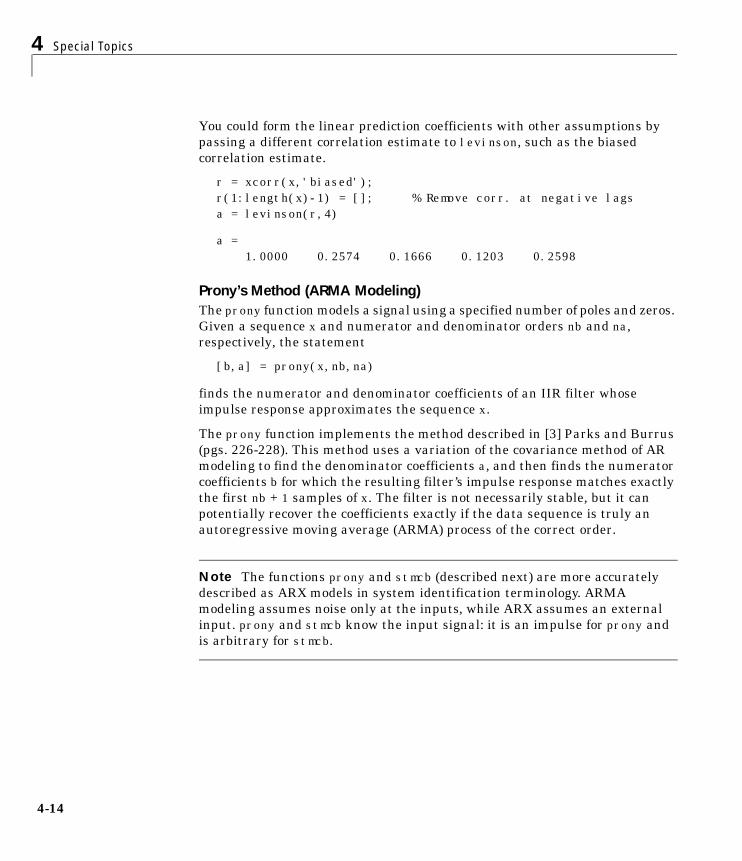
4 Special Topics
4-14
You could form the linear prediction coefficients with other assumptions bypassing a different correlation estimate to levinson, such as the biasedcorrelation estimate.
r = xcorr(x,'biased');r(1:length(x)-1) = []; % Remove corr. at negative lagsa = levinson(r,4)
a = 1.0000 0.2574 0.1666 0.1203 0.2598
Prony’s Method (ARMA Modeling)The prony function models a signal using a specified number of poles and zeros.Given a sequence x and numerator and denominator orders nb and na,respectively, the statement
[b,a] = prony(x,nb,na)
finds the numerator and denominator coefficients of an IIR filter whoseimpulse response approximates the sequence x.
The prony function implements the method described in [3] Parks and Burrus(pgs. 226-228). This method uses a variation of the covariance method of ARmodeling to find the denominator coefficients a, and then finds the numeratorcoefficients b for which the resulting filter’s impulse response matches exactlythe first nb + 1 samples of x. The filter is not necessarily stable, but it canpotentially recover the coefficients exactly if the data sequence is truly anautoregressive moving average (ARMA) process of the correct order.
Note The functions prony and stmcb (described next) are more accuratelydescribed as ARX models in system identification terminology. ARMAmodeling assumes noise only at the inputs, while ARX assumes an externalinput. prony and stmcb know the input signal: it is an impulse for prony andis arbitrary for stmcb.
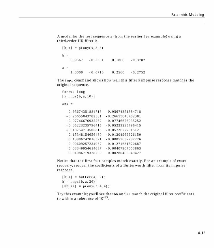
Parametric Modeling
4-15
A model for the test sequence x (from the earlier lpc example) using athird-order IIR filter is
[b,a] = prony(x,3,3)
b = 0.9567 -0.3351 0.1866 -0.3782
a = 1.0000 -0.0716 0.2560 -0.2752
The impz command shows how well this filter’s impulse response matches theoriginal sequence.
format long[x impz(b,a,10)]
ans =
0.95674351884718 0.95674351884718 -0.26655843782381 -0.26655843782381 -0.07746676935252 -0.07746676935252 -0.05223235796415 -0.05223235796415 -0.18754713506815 -0.05726777015121 0.15348154656430 -0.01204969926150 0.13986742016521 -0.00057632797226 0.00609257234067 -0.01271681570687 0.03349954614087 -0.00407967053863 0.01086719328209 0.00280486049427
Notice that the first four samples match exactly. For an example of exactrecovery, recover the coefficients of a Butterworth filter from its impulseresponse.
[b,a] = butter(4,.2);h = impz(b,a,26);[bb,aa] = prony(h,4,4);
Try this example; you’ll see that bb and aa match the original filter coefficientsto within a tolerance of 10-13.
4 Special Topics
4-16
Steiglitz-McBride Method (ARMA Modeling)The stmcb function determines the coefficients for the system b(z)/a(z) given anapproximate impulse response x, as well as the desired number of zeros andpoles. This function identifies an unknown system based on both input andoutput sequences that describe the system’s behavior, or just the impulseresponse of the system. In its default mode, stmcb works like prony.
[b,a] = stmcb(x,3,3)
b = 0.9567 -0.5181 0.5702 -0.5471
a = 1.0000 -0.2384 0.5234 -0.3065
stmcb also finds systems that match given input and output sequences.
y = filter(1,[1 1],x); % Create an output signal.[b,a] = stmcb(y,x,0,1)
b = 1.0000
a = 1 1
In this example, stmcb correctly identifies the system used to create y from x.
The Steiglitz-McBride method is a fast iterative algorithm that solves for thenumerator and denominator coefficients simultaneously in an attempt tominimize the signal error between the filter output and the given outputsignal. This algorithm usually converges rapidly, but might not converge if themodel order is too large. As for prony, stmcb’s resulting filter is not necessarilystable due to its exact modeling approach.
stmcb provides control over several important algorithmic parameters; modifythese parameters if you are having trouble modeling the data. To change thenumber of iterations from the default of five and provide an initial estimate forthe denominator coefficients
n = 10; % Number of iterationsa = lpc(x,3); % Initial estimates for denominator[b,a] = stmcb(x,3,3,n,a);

Parametric Modeling
4-17
The function uses an all-pole model created with prony as an initial estimatewhen you do not provide one of your own.
To compare the functions lpc, prony, and stmcb, compute the signal error ineach case.
a1 = lpc(x,3);[b2,a2] = prony(x,3,3);[b3,a3] = stmcb(x,3,3);[x-impz(1,a1,10) x-impz(b2,a2,10) x-impz(b3,a3,10)]
ans =
-0.0433 0 -0.0000 -0.0240 0 0.0234 -0.0040 0 -0.0778 -0.0448 -0.0000 0.0498 -0.2130 -0.1303 -0.0742 0.1545 0.1655 0.1270 0.1426 0.1404 0.1055 0.0068 0.0188 0.0465 0.0329 0.0376 0.0530 0.0108 0.0081 -0.0162
sum(ans.^2)
ans =
0.0953 0.0659 0.0471
In comparing modeling capabilities for a given order IIR model, the last resultshows that for this example, stmcb performs best, followed by prony, then lpc.This relative performance is typical of the modeling functions.
4 Special Topics
4-18
Frequency-Domain Based ModelingThe invfreqs and invfreqz functions implement the inverse operations offreqs and freqz; they find an analog or digital transfer function of a specifiedorder that matches a given complex frequency response. Though the followingexamples demonstrate invfreqz, the discussion also applies to invfreqs.
To recover the original filter coefficients from the frequency response of asimple digital filter
[b,a] = butter(4,0.4) % Design Butterworth lowpass
b = 0.0466 0.1863 0.2795 0.1863 0.0466
a = 1.0000 -0.7821 0.6800 -0.1827 0.0301
[h,w] = freqz(b,a,64); % Compute frequency response[bb,aa] = invfreqz(h,w,4,4) % Model: nb = 4, na = 4
bb =
0.0466 0.1863 0.2795 0.1863 0.0466
aa =
1.0000 -0.7821 0.6800 -0.1827 0.0301
The vector of frequencies w has the units in rad/sample, and the frequenciesneed not be equally spaced. invfreqz finds a filter of any order to fit thefrequency data; a third-order example is
[bb,aa] = invfreqz(h,w,3,3) % Find third-order IIR
bb =
0.0464 0.1785 0.2446 0.1276
aa =
1.0000 -0.9502 0.7382 -0.2006
Both invfreqs and invfreqz design filters with real coefficients; for a datapoint at positive frequency f, the functions fit the frequency response at both fand -f.
Parametric Modeling
4-19
By default invfreqz uses an equation error method to identify the best modelfrom the data. This finds b and a in
by creating a system of linear equations and solving them with MATLAB’s \operator. Here A(w(k)) and B(w(k)) are the Fourier transforms of thepolynomials a and b respectively at the frequency w(k), and n is the number offrequency points (the length of h and w). wt(k) weights the error relative to theerror at different frequencies. The syntax
invfreqz(h,w,nb,na,wt)
includes a weighting vector. In this mode, the filter resulting from invfreqz isnot guaranteed to be stable.
invfreqz provides a superior (“output-error”) algorithm that solves the directproblem of minimizing the weighted sum of the squared error between theactual frequency response points and the desired response
To use this algorithm, specify a parameter for the iteration count after theweight vector parameter
wt = ones(size(w)); % Create unity weighting vector[bbb,aaa] = invfreqz(h,w,3,3,wt,30) % 30 iterations
bbb =
0.0464 0.1829 0.2572 0.1549
aaa =
1.0000 -0.8664 0.6630 -0.1614
The resulting filter is always stable.
minb a,
wt k( ) h k( )A w k( )( ) B w k( )( )– 2
k 1=
n
minb a,
wt k( ) h k( )B w k( )( )A w k( )( )--------------------–
2
k 1=
n
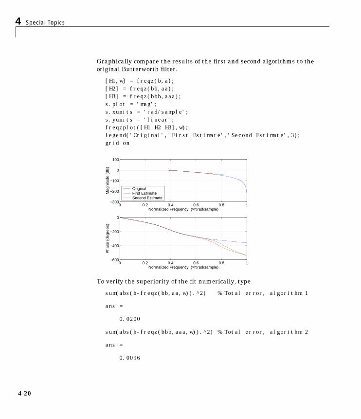
4 Special Topics
4-20
Graphically compare the results of the first and second algorithms to theoriginal Butterworth filter.
[H1,w] = freqz(b,a);[H2] = freqz(bb,aa);[H3] = freqz(bbb,aaa);s.plot = 'mag';s.xunits = 'rad/sample';s.yunits = 'linear';freqzplot([H1 H2 H3],w);legend('Original','First Estimate','Second Estimate',3);grid on
To verify the superiority of the fit numerically, type
sum(abs(h-freqz(bb,aa,w)).^2) % Total error, algorithm 1
ans =
0.0200
sum(abs(h-freqz(bbb,aaa,w)).^2) % Total error, algorithm 2
ans =
0.0096
0 0.2 0.4 0.6 0.8 1−600
−400
−200
0
Normalized Frequency (×π rad/sample)
Pha
se (
degr
ees)
0 0.2 0.4 0.6 0.8 1−300
−200
−100
0
100
Normalized Frequency (×π rad/sample)
Mag
nitu
de (
dB)
OriginalFirst EstimateSecond Estimate
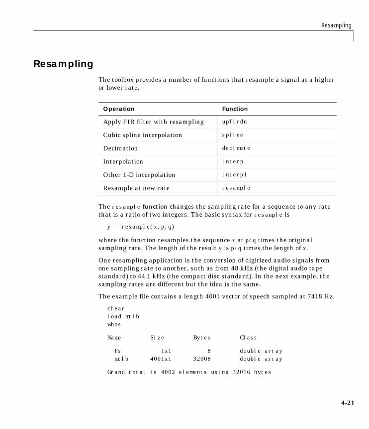
Resampling
4-21
ResamplingThe toolbox provides a number of functions that resample a signal at a higheror lower rate.
The resample function changes the sampling rate for a sequence to any ratethat is a ratio of two integers. The basic syntax for resample is
y = resample(x,p,q)
where the function resamples the sequence x at p/q times the originalsampling rate. The length of the result y is p/q times the length of x.
One resampling application is the conversion of digitized audio signals fromone sampling rate to another, such as from 48 kHz (the digital audio tapestandard) to 44.1 kHz (the compact disc standard). In the next example, thesampling rates are different but the idea is the same.
The example file contains a length 4001 vector of speech sampled at 7418 Hz.
clearload mtlbwhos
Name Size Bytes Class
Fs 1x1 8 double array mtlb 4001x1 32008 double array
Grand total is 4002 elements using 32016 bytes
Operation Function
Apply FIR filter with resampling upfirdn
Cubic spline interpolation spline
Decimation decimate
Interpolation interp
Other 1-D interpolation interp1
Resample at new rate resample
4 Special Topics
4-22
FsFs = 7418
To play this speech signal on a workstation that can only play sound at8192 Hz, use the rat function to find integers p and q that yield the correctresampling factor.
[p,q] = rat(8192/Fs,0.0001)
p = 127
q = 115
Since p/q*Fs = 8192.05 Hz, the tolerance of 0.0001 is acceptable; to resamplethe signal at very close to 8192 Hz.
y = resample(mtlb,p,q);
resample applies a lowpass filter to the input sequence to prevent aliasingduring resampling. It designs this filter using the firls function with a Kaiserwindow. The syntax
resample(x,p,q,l,beta)
controls the filter’s length and the beta parameter of the Kaiser window.Alternatively, use the function intfilt to design an interpolation filter b anduse it with
resample(x,p,q,b)
The decimate and interp functions do the same thing as resample with p = 1and q = 1, respectively. These functions provide different anti-alias filteringoptions, and they incur a slight signal delay due to filtering. The interpfunction is significantly less efficient than the resample function with q = 1.
The toolbox also contains a function, upfirdn, that applies an FIR filter to aninput sequence and outputs the filtered sequence at a different sample ratethan its original rate. See “Multirate Filter Bank Implementation” on page1-20 and the description of upfirdn in Chapter 7, “Function Reference,” formore details.

Resampling
4-23
The standard MATLAB environment contains a function, spline, that workswith irregularly spaced data. The MATLAB function interp1 performsinterpolation, or table lookup, using various methods including linear andcubic interpolation. See the MATLAB documentation for information onspline and interp1.

4 Special Topics
4-24
Cepstrum AnalysisCepstrum analysis is a nonlinear signal processing technique with a variety ofapplications in areas such as speech and image processing. The SignalProcessing Toolbox provides three functions for cepstrum analysis.
The complex cepstrum for a sequence x is calculated by finding the complexnatural logarithm of the Fourier transform of x, then the inverse Fouriertransform of the resulting sequence.
The toolbox function cceps performs this operation, estimating the complexcepstrum for an input sequence. It returns a real sequence the same size as theinput sequence.
xhat = cceps(x)
The complex cepstrum transformation is central to the theory and applicationof homomorphic systems, that is, systems that obey certain general rules ofsuperposition. See Oppenheim and Schafer [2] for a discussion of the complexcepstrum and homomorphic transformations, with details on speech processingapplications.
Try using cceps in an echo detection application. First, create a 45 Hz sinewave sampled at 100 Hz.
t = 0:0.01:1.27;s1 = sin(2*pi*45*t);
Operation Function
Complex cepstrum cceps
Inverse complex cepstrum icceps
Real cepstrum rceps
x 12π------ X ejω( )[ ]log ejωn ωd
π–
π
=
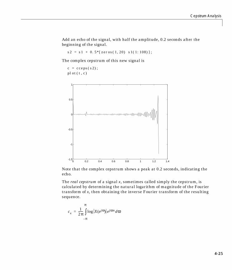
Cepstrum Analysis
4-25
Add an echo of the signal, with half the amplitude, 0.2 seconds after thebeginning of the signal.
s2 = s1 + 0.5*[zeros(1,20) s1(1:108)];
The complex cepstrum of this new signal is
c = cceps(s2);plot(t,c)
Note that the complex cepstrum shows a peak at 0.2 seconds, indicating theecho.
The real cepstrum of a signal x, sometimes called simply the cepstrum, iscalculated by determining the natural logarithm of magnitude of the Fouriertransform of x, then obtaining the inverse Fourier transform of the resultingsequence.
0 0.2 0.4 0.6 0.8 1 1.2 1.4-1.5
-1
-0.5
0
0.5
1
cx1
2π------ X ejω( )log ejωn ωd
π–
π
=
4 Special Topics
4-26
The toolbox function rceps performs this operation, returning the realcepstrum for a sequence x. The returned sequence is a real-valued vector thesame size as the input vector.
y = rceps(x)
By definition, you cannot reconstruct the original sequence from its realcepstrum transformation, as the real cepstrum is based only on the magnitudeof the Fourier transform for the sequence (see Oppenheim and Schafer [2]). Therceps function, however, can reconstruct a minimum-phase version of theoriginal sequence by applying a windowing function in the cepstral domain. Toobtain both the real cepstrum and the minimum phase reconstruction for asequence, use
[y,ym] = rceps(x)
where y is the real cepstrum and ym is the minimum phase reconstruction of x.
Inverse Complex CepstrumTo invert the complex cepstrum, use the icceps function. Inversion iscomplicated by the fact that the cceps function performs a data dependentphase modification so that the unwrapped phase of its input is continuous atzero frequency. The phase modification is equivalent to an integer delay. Thisdelay term is returned by cceps if you ask for a second output. For example,
x = 1:10;[xh,nd] = cceps(x)
xh = Columns 1 through 7 2.2428 -0.0420 -0.0210 0.0045 0.0366 0.0788 0.1386 Columns 8 through 10 0.2327 0.4114 0.9249
nd = 1
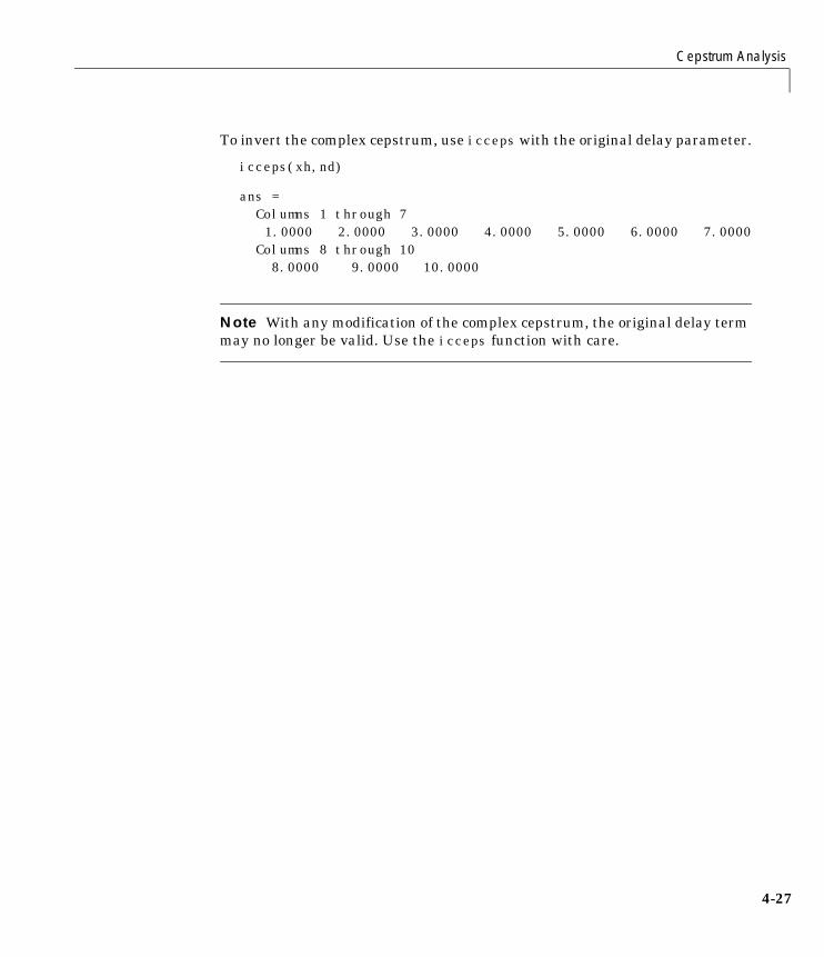
Cepstrum Analysis
4-27
To invert the complex cepstrum, use icceps with the original delay parameter.
icceps(xh,nd)
ans = Columns 1 through 7 1.0000 2.0000 3.0000 4.0000 5.0000 6.0000 7.0000 Columns 8 through 10 8.0000 9.0000 10.0000
Note With any modification of the complex cepstrum, the original delay termmay no longer be valid. Use the icceps function with care.

4 Special Topics
4-28
FFT-Based Time-Frequency AnalysisThe Signal Processing Toolbox provides a function, specgram, that returns thetime-dependent Fourier transform for a sequence, or displays this informationas a spectrogram. The time-dependent Fourier transform is the discrete-timeFourier transform for a sequence, computed using a sliding window. This formof the Fourier transform, also known as the short-time Fourier transform(STFT), has numerous applications in speech, sonar, and radar processing. Thespectrogram of a sequence is the magnitude of the time-dependent Fouriertransform versus time.
To display the spectrogram of a linear FM signal
fs = 10000;t = 0:1/fs:2;x = vco(sawtooth(2*pi*t,.75),[0.1 0.4]*fs,fs);specgram(x,512,fs,kaiser(256,5),220)
Note that the spectrogram display is an image, not a plot.
Time
Fre
quen
cy
0 0.2 0.4 0.6 0.8 1 1.2 1.4 1.6 1.80
500
1000
1500
2000
2500
3000
3500
4000
4500
5000

Median Filtering
4-29
Median FilteringThe function medfilt1 implements one-dimensional median filtering, anonlinear technique that applies a sliding window to a sequence. The medianfilter replaces the center value in the window with the median value of all thepoints within the window [4]. In computing this median, medfilt1 assumeszeros beyond the input points.
When the number of elements n in the window is even, medfilt1 sorts thenumbers, then takes the average of the (n-1)/2 and (n-1)/2 + 1 elements.
Two simple examples with fourth- and third-order median filters are
medfilt1([4 3 5 2 8 9 1],4)
ans =
1.500 3.500 3.500 4.000 6.500 5.000 4.500
medfilt1([4 3 5 2 8 9 1],3)
ans =
3 4 3 5 8 8 1
See the Image Processing Toolbox User’s Guide for information ontwo-dimensional median filtering.
4 Special Topics
4-30
Communications ApplicationsThe toolbox provides three functions for communications simulation.
Modulation varies the amplitude, phase, or frequency of a carrier signal withreference to a message signal. The modulate function modulates a messagesignal with a specified modulation method.
The basic syntax for the modulate function is
y = modulate(x,fc,fs,'method',opt)
where:
• x is the message signal.
• fc is the carrier frequency.
• fs is the sampling frequency.
• method is a flag for the desired modulation method.
• opt is any additional argument that the method requires. (Not allmodulation methods require an option argument.)
The table below summarizes the modulation methods provided; see thedocumentation for modulate, demod, and vco for complete details on each.
Operation Function
Modulation modulate
Demodulation demod
Voltage controlled oscillation vco
Method Description
amdsb-sc or am Amplitude modulation, double side-band, suppressedcarrier
amdsb-tc Amplitude modulation, double side-band, transmittedcarrier
Communications Applications
4-31
If the input x is an array rather than a vector, modulate modulates eachcolumn of the array.
To obtain the time vector that modulate uses to compute the modulated signal,specify a second output parameter.
[y,t] = modulate(x,fc,fs,'method',opt)
The demod function performs demodulation, that is, it obtains the originalmessage signal from the modulated signal.
The syntax for demod is
x = demod(y,fc,fs,'method',opt)
demod uses any of the methods shown for modulate, but the syntax forquadrature amplitude demodulation requires two output parameters.
[X1,X2] = demod(y,fc,fs,'qam')
If the input y is an array, demod demodulates all columns.
Try modulating and demodulating a signal. A 50 Hz sine wave sampled at1000 Hz is
t = (0:1/1000:2);x = sin(2*pi*50*t);
amssb Amplitude modulation, single side-band
fm Frequency modulation
pm Phase modulation
ptm Pulse time modulation
pwm Pulse width modulation
qam Quadrature amplitude modulation
Method Description
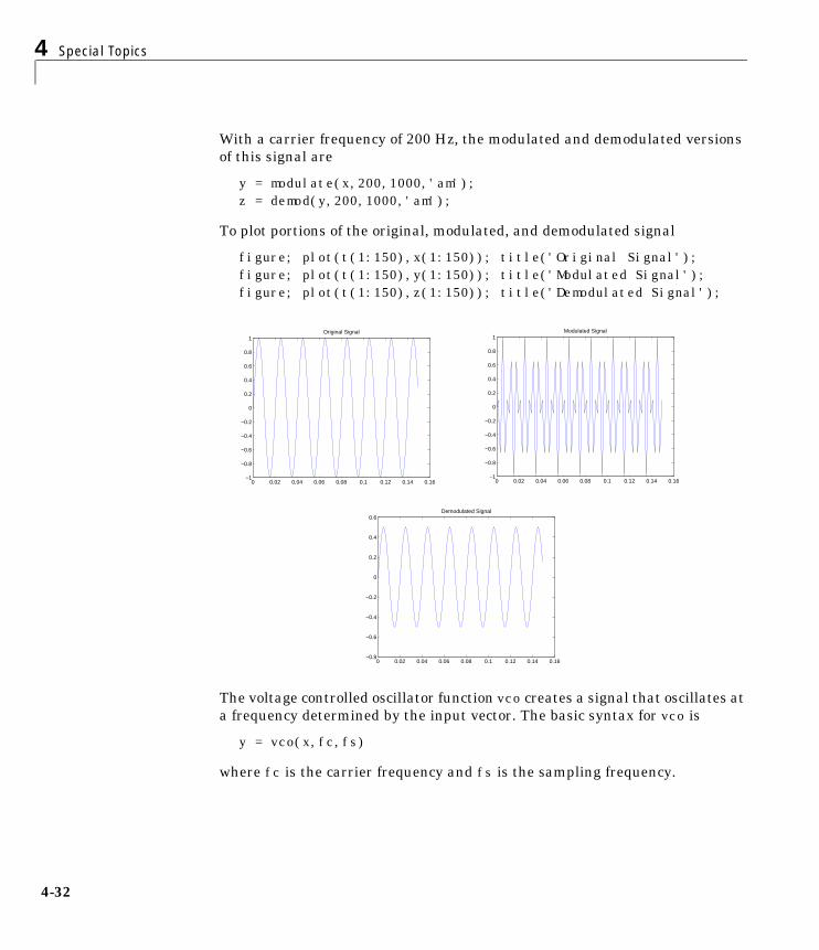
4 Special Topics
4-32
With a carrier frequency of 200 Hz, the modulated and demodulated versionsof this signal are
y = modulate(x,200,1000,'am');z = demod(y,200,1000,'am');
To plot portions of the original, modulated, and demodulated signal
figure; plot(t(1:150),x(1:150)); title('Original Signal');figure; plot(t(1:150),y(1:150)); title('Modulated Signal');figure; plot(t(1:150),z(1:150)); title('Demodulated Signal');
The voltage controlled oscillator function vco creates a signal that oscillates ata frequency determined by the input vector. The basic syntax for vco is
y = vco(x,fc,fs)
where fc is the carrier frequency and fs is the sampling frequency.
0 0.02 0.04 0.06 0.08 0.1 0.12 0.14 0.16−1
−0.8
−0.6
−0.4
−0.2
0
0.2
0.4
0.6
0.8
1Original Signal
0 0.02 0.04 0.06 0.08 0.1 0.12 0.14 0.16−1
−0.8
−0.6
−0.4
−0.2
0
0.2
0.4
0.6
0.8
1Modulated Signal
0 0.02 0.04 0.06 0.08 0.1 0.12 0.14 0.16−0.8
−0.6
−0.4
−0.2
0
0.2
0.4
0.6Demodulated Signal

Communications Applications
4-33
To scale the frequency modulation range, use
y = vco(x,[Fmin Fmax],fs)
In this case, vco scales the frequency modulation range so values of x on theinterval [-1 1] map to oscillations of frequency on [Fmin Fmax].
If the input x is an array, vco produces an array whose columns oscillateaccording to the columns of x.
See “FFT-Based Time-Frequency Analysis” on page 4-28 for an example usingthe vco function.
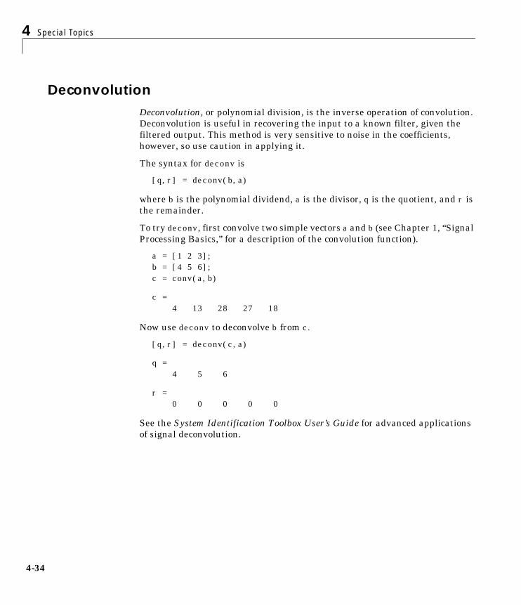
4 Special Topics
4-34
DeconvolutionDeconvolution, or polynomial division, is the inverse operation of convolution.Deconvolution is useful in recovering the input to a known filter, given thefiltered output. This method is very sensitive to noise in the coefficients,however, so use caution in applying it.
The syntax for deconv is
[q,r] = deconv(b,a)
where b is the polynomial dividend, a is the divisor, q is the quotient, and r isthe remainder.
To try deconv, first convolve two simple vectors a and b (see Chapter 1, “SignalProcessing Basics,” for a description of the convolution function).
a = [1 2 3];b = [4 5 6];c = conv(a,b)
c = 4 13 28 27 18
Now use deconv to deconvolve b from c.
[q,r] = deconv(c,a)
q = 4 5 6
r = 0 0 0 0 0
See the System Identification Toolbox User’s Guide for advanced applicationsof signal deconvolution.

Specialized Transforms
4-35
Specialized TransformsIn addition to the discrete Fourier transform (DFT) described in Chapter 1,“Signal Processing Basics,” the Signal Processing Toolbox and the MATLABenvironment together provide the following transform functions:
• The chirp z-transform (CZT), useful in evaluating the z-transform alongcontours other than the unit circle. The chirp z-transform is also moreefficient than the DFT algorithm for the computation of prime-lengthtransforms, and it is useful in computing a subset of the DFT for a sequence.
• The discrete cosine transform (DCT), closely related to the DFT. The DCT’senergy compaction properties are useful for applications like signal coding.
• The Hilbert transform, which facilitates the formation of the analytic signal.The analytic signal is useful in the area of communications, particularly inbandpass signal processing.
Chirp z-TransformThe chirp z-transform, or CZT, computes the z-transform along spiral contoursin the z-plane for an input sequence. Unlike the DFT, the CZT is notconstrained to operate along the unit circle, but can evaluate the z-transformalong contours described by
where A is the complex starting point, W is a complex scalar describing thecomplex ratio between points on the contour, and M is the length of thetransform.
One possible spiral is
A = 0.8*exp(j*pi/6);W = 0.995*exp(-j*pi*.05);M = 91;z = A*(W.^(-(0:M-1)));zplane([],z.')
zl AW l– l 0 … M 1–, ,=,=

4 Special Topics
4-36
czt(x,M,W,A) computes the z-transform of x on these points.
An interesting and useful spiral set is m evenly spaced samples around the unitcircle, parameterized by A = 1 and W = exp(-j*pi/M). The z-transform on thiscontour is simply the DFT, obtained by
y = czt(x)
czt may be faster than the fft function for computing the DFT of sequenceswith certain odd lengths, particularly long prime-length sequences.
-1.5 -1 -0.5 0 0.5 1 1.5
-1
-0.5
0
0.5
1
Real part
Imag
inar
y pa
rt
Specialized Transforms
4-37
Discrete Cosine TransformThe toolbox function dct computes the unitary discrete cosine transform, orDCT, for an input vector or matrix. Mathematically, the unitary DCT of aninput sequence x is
where
The DCT is closely related to the discrete Fourier transform; the DFT isactually one step in the computation of the DCT for a sequence. The DCT,however, has better energy compaction properties, with just a few of thetransform coefficients representing the majority of the energy in the sequence.The energy compaction properties of the DCT make it useful in applicationssuch as data communications.
The function idct computes the inverse DCT for an input sequence,reconstructing a signal from a complete or partial set of DCT coefficients. Theinverse discrete cosine transform is
where
y k( ) w k( ) x n( ) π 2n 1–( ) k 1–( )2N
-------------------------------------------cos
n 1=
N
k 1 … N, ,=,=
w k( )
1N
--------- k 1=,
2N---- 2 k N≤ ≤,
=
x n( ) w n( ) y k( ) π 2n 1–( ) k 1–( )2N
-------------------------------------------cos
k 1=
N
n 1 … N, ,=,=
w n( )
1N
--------- n 1=,
2N---- 2 n N≤ ≤,
=

4 Special Topics
4-38
Because of the energy compaction mentioned above, it is possible to reconstructa signal from only a fraction of its DCT coefficients. For example, generate a25 Hz sinusoidal sequence, sampled at 1000 Hz.
t = (0:1/999:1);x = sin(2*pi*25*t);
Compute the DCT of this sequence and reconstruct the signal using only thosecomponents with value greater than 0.1 (64 of the original 1000 DCTcoefficients).
y = dct(x) % Compute DCTy2 = find(abs(y) < 0.9); % Use 17 coefficientsy(y2) = zeros(size(y2)); % Zero out points < 0.9z = idct(y); % Reconstruct signal using inverse DCT
Plot the original and reconstructed sequences.
subplot(2,1,1); plot(t,x);title('Original Signal')subplot(2,1,2); plot(t,z), axis([0 1 -1 1])title('Reconstructed Signal')
0 0.2 0.4 0.6 0.8 1−1
−0.5
0
0.5
1Original Signal
0 0.2 0.4 0.6 0.8 1−1
−0.5
0
0.5
1Reconstructed Signal

Specialized Transforms
4-39
One measure of the accuracy of the reconstruction is
norm(x-z)/norm(x)
that is, the norm of the difference between the original and reconstructedsignals, divided by the norm of the original signal. In this case, the relativeerror of reconstruction is 0.1443. The reconstructed signal retainsapproximately 85% of the energy in the original signal.
Hilbert TransformThe toolbox function hilbert computes the Hilbert transform for a real inputsequence x and returns a complex result of the same length
y = hilbert(x)
where the real part of y is the original real data and the imaginary part is theactual Hilbert transform. y is sometimes called the analytic signal, in referenceto the continuous-time analytic signal. A key property of the discrete-timeanalytic signal is that its z-transform is 0 on the lower half of the unit circle.Many applications of the analytic signal are related to this property; forexample, the analytic signal is useful in avoiding aliasing effects for bandpasssampling operations. The magnitude of the analytic signal is the complexenvelope of the original signal.
The Hilbert transform is related to the actual data by a 90° phase shift; sinesbecome cosines and vice versa. To plot a portion of data (solid line) and itsHilbert transform (dotted line)
t = (0:1/1023:1);x = sin(2*pi*60*t);y = hilbert(x);plot(t(1:50),real(y(1:50))), hold onplot(t(1:50),imag(y(1:50)),':'), hold off
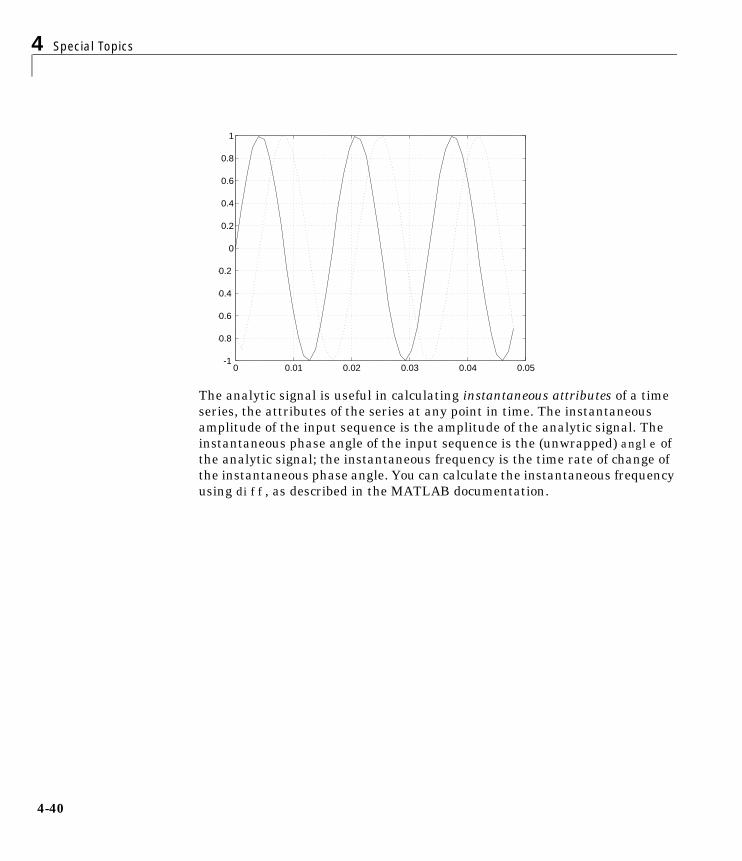
4 Special Topics
4-40
The analytic signal is useful in calculating instantaneous attributes of a timeseries, the attributes of the series at any point in time. The instantaneousamplitude of the input sequence is the amplitude of the analytic signal. Theinstantaneous phase angle of the input sequence is the (unwrapped) angle ofthe analytic signal; the instantaneous frequency is the time rate of change ofthe instantaneous phase angle. You can calculate the instantaneous frequencyusing diff, as described in the MATLAB documentation.
0 0.01 0.02 0.03 0.04 0.05-1
-0.8
-0.6
-0.4
-0.2
0
0.2
0.4
0.6
0.8
1

Selected Bibliography
4-41
Selected Bibliography[1] Kay, S.M. Modern Spectral Estimation. Englewood Cliffs, NJ: Prentice Hall,1988.
[2] Oppenheim, A.V., and R.W. Schafer. Discrete-Time Signal Processing.Englewood Cliffs, NJ: Prentice Hall, 1989.
[3] Parks, T.W., and C.S. Burrus. Digital Filter Design. New York: John Wiley& Sons, 1987.
[4] Pratt,W.K. Digital Image Processing. New York: John Wiley & Sons, 1991.

4 Special Topics
4-42

5Filter Design and AnalysisTool
Overview . . . . . . . . . . . . . . . . . . . . . 5-2
Opening the Filter Design and Analysis Tool . . . . . 5-5
Getting Help . . . . . . . . . . . . . . . . . . . . 5-6
Choosing a Filter Type . . . . . . . . . . . . . . . 5-7
Choosing a Filter Design Method . . . . . . . . . . 5-8
Setting the Filter Design Specifications . . . . . . . 5-9
Computing the Filter Coefficients . . . . . . . . . . 5-12
Analyzing the Filter . . . . . . . . . . . . . . . . 5-13
Converting the Filter Structure . . . . . . . . . . . 5-14
Importing a Filter Design . . . . . . . . . . . . . . 5-16
Exporting a Filter Design . . . . . . . . . . . . . . 5-19
Saving and Opening Filter Design Sessions . . . . . . 5-21

5 Filter Design and Analysis Tool
5-2
OverviewYou can use the Filter Design and Analysis Tool (FDATool) as a convenientalternative to the command line filter design functions. This chapter containsthe following sections, which walk you through a typical filter design sessionusing the FDATool:
• “Opening the Filter Design and Analysis Tool”
• “Getting Help”
• “Choosing a Filter Type”
• “Choosing a Filter Design Method”
• “Setting the Filter Design Specifications”
• “Computing the Filter Coefficients”
• “Analyzing the Filter”
• “Converting the Filter Structure”
• “Importing a Filter Design”
• “Exporting a Filter Design”
• “Saving and Opening Filter Design Sessions”
Below is a brief introduction to the FDATool that will give you a betterunderstanding of how it can be used.
Filter Design MethodsThe tool gives you access to all of the filter design methods in the SignalProcessing Toolbox:
• Butterworth (butter)
• Chebyshev type I (cheby1)
• Chebyshev type II (cheby2)
• Elliptic (ellip)
• Equiripple (remez)
• Least squares (firls)
• Windows
- Bartlett (bartlett, fir2)
- Blackman (blackman, fir2)

5-3
- Boxcar (boxcar, fir2)
- Chebyshev (chebwin, fir2)
- Hamming (hamming, fir2)
- Hann (hann, fir2)
- Kaiser (kaiser, fir1)
- Triangular (triang, fir1)
Additional filter design methods are available to users of the Filter DesignToolbox.
Using the Filter Design and Analysis ToolThere are different ways that you can design filters using the Filter Design andAnalysis Tool. For example:
• You can first choose a filter type, such as bandpass, and then choose from theavailable FIR or IIR filter design methods.
• You can specify the filter by its type alone, along with certain frequency- ortime-domain specifications such as passband frequencies and stopbandfrequencies. The filter you design is then computed using the default filterdesign method and filter order.
Analyzing Filter ResponsesOnce you have designed your filter, you can analyze different filter responses:
• Magnitude response (freqz)
• Phase response (freqz)
• Pole-zero plots (zplane)
• Impulse response (impz)
• Group delay (grpdelay)
• Step response
You can also display the filter coefficients.
Filter Design and Analysis Tool ModesThe Filter Design and Analysis Tool operates in two modes:

5 Filter Design and Analysis Tool
5-4
• Design mode. In this mode, you can:
- Design filters from scratch.
- Modify existing filters designed by FDATool.
- Analyze filters.
• Import mode. In this mode, you can:
- Import previously saved filters or filter coefficients that you have stored inthe MATLAB workspace.
- Analyze imported filters.
There is one more mode available to you if you also have the Filter DesignToolbox: the quantize mode. Use this mode to:
• Quantize double-precision filters that you design in FDATool.
• Quantize double-precision filters that you import into FDATool.
• Analyze quantized filters.
Getting HelpAt any time, you can right-click or press the What’s this? button, , to getinformation on the different parts of the GUI.

Opening the Filter Design and Analysis Tool
5-5
Opening the Filter Design and Analysis ToolTo open the Filter Design and Analysis Tool, type
fdatool
The Filter Design and Analysis Tool opens in the default design mode.
Choose an analysis method for analyzing the filter design.
Choose the type of filter to design.
Choose the filter design method to use
Press Design Filter to compute the filter coefficients.
Select the What’s this? button and click on a region of the GUI to access context-sensitive help.
Set quantization parameters for the Filter Design Toolbox.
Set filter specifications. These depend on the type of filter you are designing, as well as the design method you specify.
Specify a filter order or allow it to be estimated.
Zoom in/out.
Use the Filter menu to choose between importing filter coefficients from the MATLAB workspace and designing the filter in the GUI.
Set window specifications for the FIR Window design.
Quantize the current filter using the Filter Design Toolbox.

5 Filter Design and Analysis Tool
5-6
Getting HelpUse the What’s this? button to find out more information about a particularregion of FDATool.
Context-Sensitive Help: The What’s This? ButtonTo find information on a particular region of the GUI:
1 Select the What’s this? button with your mouse.
2 Click on the region of the GUI you want information on.
You can also right-click a region of the GUI or select What’s this? from theHelp menu to launch context-sensitive help.
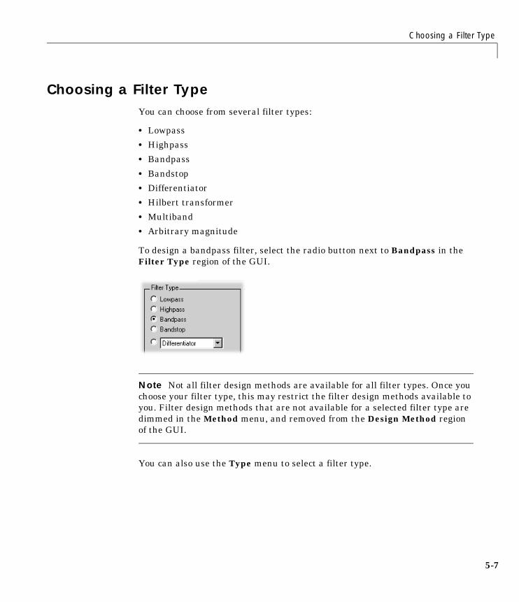
Choosing a Filter Type
5-7
Choosing a Filter TypeYou can choose from several filter types:
• Lowpass
• Highpass
• Bandpass
• Bandstop
• Differentiator
• Hilbert transformer
• Multiband
• Arbitrary magnitude
To design a bandpass filter, select the radio button next to Bandpass in theFilter Type region of the GUI.
Note Not all filter design methods are available for all filter types. Once youchoose your filter type, this may restrict the filter design methods available toyou. Filter design methods that are not available for a selected filter type aredimmed in the Method menu, and removed from the Design Method regionof the GUI.
You can also use the Type menu to select a filter type.

5 Filter Design and Analysis Tool
5-8
Choosing a Filter Design MethodYou can use the default filter design method for the filter type that you’veselected, or you can select a filter design method from the available FIR and IIRmethods listed in the GUI.
To select the Remez algorithm to compute FIR filter coefficients, select the FIRradio button and choose Equiripple from the list of methods.
You can also use the Method menu to select a filter design method.

Setting the Filter Design Specifications
5-9
Setting the Filter Design SpecificationsThe filter design specifications that you can set vary according to filter type anddesign method. For example, to design a bandpass filter, you can enter:
• Frequency specifications
• Magnitude specifications
• Filter order
The display region illustrates filter specifications when you select FilterSpecifications from the Analysis menu.
Bandpass Filter Frequency SpecificationsFor a bandpass filter, you can set:
• Units of frequency:
- Hz
- kHz
- MHz
- Normalized (0 to 1)
• Sampling frequency
• Passband frequencies
• Stopband frequencies

5 Filter Design and Analysis Tool
5-10
You specify the passband with two frequencies. The first frequency determinesthe lower edge of the passband, and the second frequency determines the upperedge of the passband.
Similarly, you specify the stopband with two frequencies. The first frequencydetermines the upper edge of the first stopband, and the second frequencydetermines the lower edge of the second stopband.
For this example:
• Keep the units in Hz (default).
• Set the sampling frequency (Fs) to 2000 Hz.
• Set the end of the first stopband (Fstop1) to 200 Hz.
• Set the beginning of the passband (Fpass1) to 300 Hz.
• Set the end of the passband (Fpass2) to 700 Hz.
• Set the beginning of the second stopband (Fstop2) to 800 Hz.
Bandpass Filter Magnitude SpecificationsFor a bandpass filter, you can specify the following magnitude responsecharacteristics:
• Units for the magnitude response (dB or linear)
• Passband ripple
• Stopband attenuation
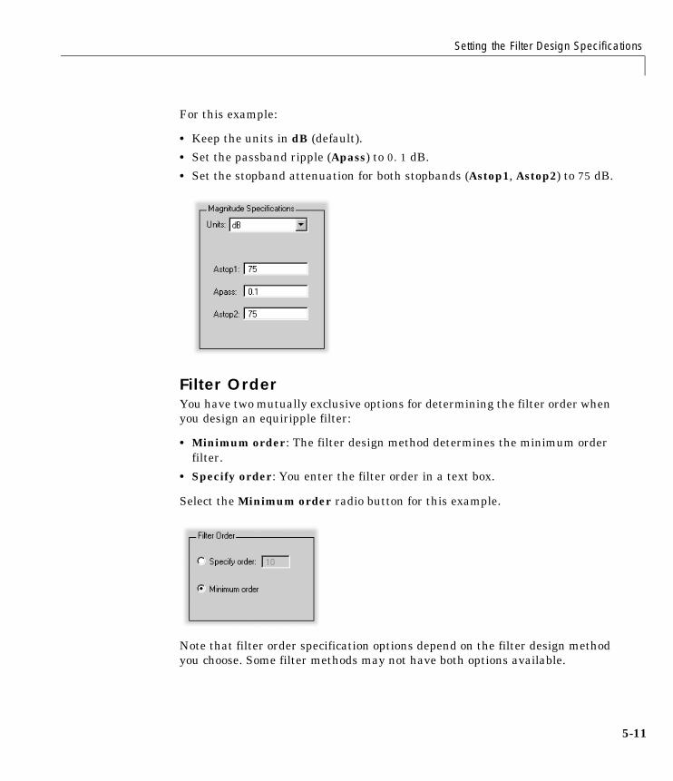
Setting the Filter Design Specifications
5-11
For this example:
• Keep the units in dB (default).
• Set the passband ripple (Apass) to 0.1 dB.
• Set the stopband attenuation for both stopbands (Astop1, Astop2) to 75 dB.
Filter OrderYou have two mutually exclusive options for determining the filter order whenyou design an equiripple filter:
• Minimum order: The filter design method determines the minimum orderfilter.
• Specify order: You enter the filter order in a text box.
Select the Minimum order radio button for this example.
Note that filter order specification options depend on the filter design methodyou choose. Some filter methods may not have both options available.

5 Filter Design and Analysis Tool
5-12
Computing the Filter CoefficientsNow that you’ve specified the filter design, select the Design Filter button tocompute the filter coefficients.
Notice that the Design Filter button is dimmed once you’ve computed thecoefficients for your filter design. This button is enabled again once you makeany changes to the filter specifications.
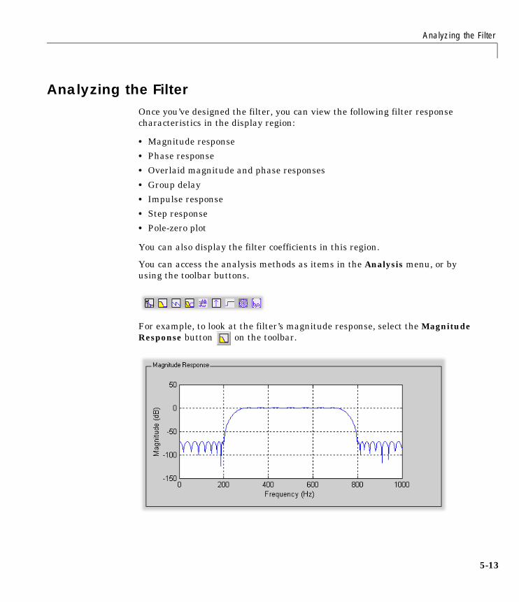
Analyzing the Filter
5-13
Analyzing the FilterOnce you’ve designed the filter, you can view the following filter responsecharacteristics in the display region:
• Magnitude response
• Phase response
• Overlaid magnitude and phase responses
• Group delay
• Impulse response
• Step response
• Pole-zero plot
You can also display the filter coefficients in this region.
You can access the analysis methods as items in the Analysis menu, or byusing the toolbar buttons.
For example, to look at the filter’s magnitude response, select the MagnitudeResponse button on the toolbar.
5 Filter Design and Analysis Tool
5-14
Converting the Filter StructureYou can use the Convert structure button to convert the current filter to a newstructure. All filters can be converted to the following representations:
• Direct form I
• Direct form II
• Direct form I transposed
• Direct form II transposed
• State-space
• Lattice ARMA
In addition, the following conversions are available for particular classes offilters:
• Minimum phase FIR filters can be converted to Lattice MA (min. phase)
• Maximum phase FIR filters can be converted to Lattice MA (max. phase)
• Allpass filters can be converted to Lattice allpass
• IIR filters can be converted to Lattice ARMA
When selected, the Use second-order sections check box instructs the tool tostore the converted filter structure as a collection of second-order sectionsrather than as a monolithic higher-order structure. The subordinate Scalemenu lets you select from the following options.
• None (default)
• L-2 (L2 norm)
• L-infinity (L∞ norm)
The ordering of the second-order sections is optimized for the selected scalingoption. (The tf2sos function that performs the conversion is called with option'down' for L2 norm scaling, and with option 'up' for L∞ norm scaling.)
For example:
• Press the Convert structure button to open the Convert structure dialogbox.
• Select Direct form I in the list of filter structures.

Converting the Filter Structure
5-15
• Select the Use second-order sections check box.
• Select L-infinity from the Scale menu for L∞ norm scaling.
5 Filter Design and Analysis Tool
5-16
Importing a Filter DesignThe Import Filter region allows you to import a filter by specifying the filtercoefficients, either by entering them explicitly or by referring to variables inthe MATLAB workspace. You can access this region by selecting Import Filterfrom the Filter menu, or by pressing Ctrl+I.
The imported filter can be in any of the representations listed in the FilterStructure menu, and described in “Filter Structures” below:
• Direct form I
• Direct form II
• Direct form I transposed
• Direct form II transposed
• Direct form II (Second-order sections)
• State-space
• Lattice allpass
• Lattice MA min. phase
• Lattice MA max. phase
• Lattice ARMA
• Quantized filter (Qfilt object) — available only when Filter DesignToolbox is installed
Select the frequency units from among the following options in the Units menu,and specify the value of the sampling frequency in the Fs field.
To import the filter, press the Import Filter button. The Display Region isautomatically updated when the new filter has been imported.

Importing a Filter Design
5-17
Filter StructuresThe structure that you choose determines the type of coefficients that you needto specify in the text fields to the right:
Direct FormFor Direct Form I, Direct Form II, Direct Form I transposed, and DirectForm II transposed, specify the filter by its transfer function representation:
• The Numerator field specifies a variable name or value for the numeratorcoefficient vector b, which contains m+1 coefficients in descending powers of z.
• The Denominator field specifies a variable name or value for thedenominator coefficient vector a, which contains n+1 coefficients indescending powers of z. For FIR filters, the Denominator is 1.
Filters in transfer function form can be produced by all of the Signal ProcessingToolbox filter design functions (e.g., fir1, fir2, remez, butter, yulewalk). See“Transfer Function” on page 1-33 for more information.
Direct Form II (Second-Order Sections)For Direct form II (Second-order sections), specify the filter by itssecond-order section representation:
The Gain field specifies a variable name or a value for the gain g, and the SOSMatrix field specifies a variable name or a value for the L-by-6 SOS matrix
H z( )B z( )A z( )-----------
b 1( ) b 2( )z 1– b m 1+( )z m–+ + +a 1( ) a 2( )z 1– a n 1+( )z n–+ + +---------------------------------------------------------------------------------------= =
H z( ) g Hk z( )
k 1=
L
∏ gb0k b1kz 1– b2kz 2–+ +
1 a1kz 1– a2kz 2–+ +----------------------------------------------------------
k 1=
L
∏= =
SOS
b01 b11 b21 1 a11 a21
b02 b12 b22 1 a12 a22
b0L b1L b2L 1 a1L a2L
=

5 Filter Design and Analysis Tool
5-18
whose rows contain the numerator and denominator coefficients bik and aik ofthe second-order sections of H(z).
Filters in second-order section form can be produced by functions such astf2sos, zp2sos, ss2sos, and sosfilt. See “Second-Order Sections (SOS)” onpage 1-38 for more information.
State-SpaceFor State-Space, specify the filter by its state-space representation:
The A, B, C, and D fields each specify a variable name or a value for thematrices in this system.
Filters in state-space form can be produced by functions such as tf2ss andzp2ss. See “State-Space” on page 1-35 for more information.
LatticeFor Lattice allpass, Lattice MA, and Lattice ARMA filters, specify the filterby its lattice representation:
• For Lattice allpass, the Lattice coeff field specifies the lattice (reflection)coefficients, k(1) to k(N), were N is the filter order.
• For Lattice MA (minimum or maximum phase), the Lattice coeff fieldspecifies the lattice (reflection) coefficients, k(1) to k(N), were N is the filterorder.
• For Lattice ARMA, the Lattice coeff field specifies the lattice (reflection)coefficients, k(1) to k(N), and the Ladder coeff field specifies the laddercoefficients, v(1) to v(N+1), were N is the filter order.
Filters in lattice form can be produced by tf2latc. See “Lattice Structure” onpage 1-38 for more information.
Quantized Filter (Qfilt Object)For Quantized filter, specify the filter as a Qfilt object. See qfilt in the FilterDesign Toolbox for more information.
x· Ax Bu+=
y Cx Du+=
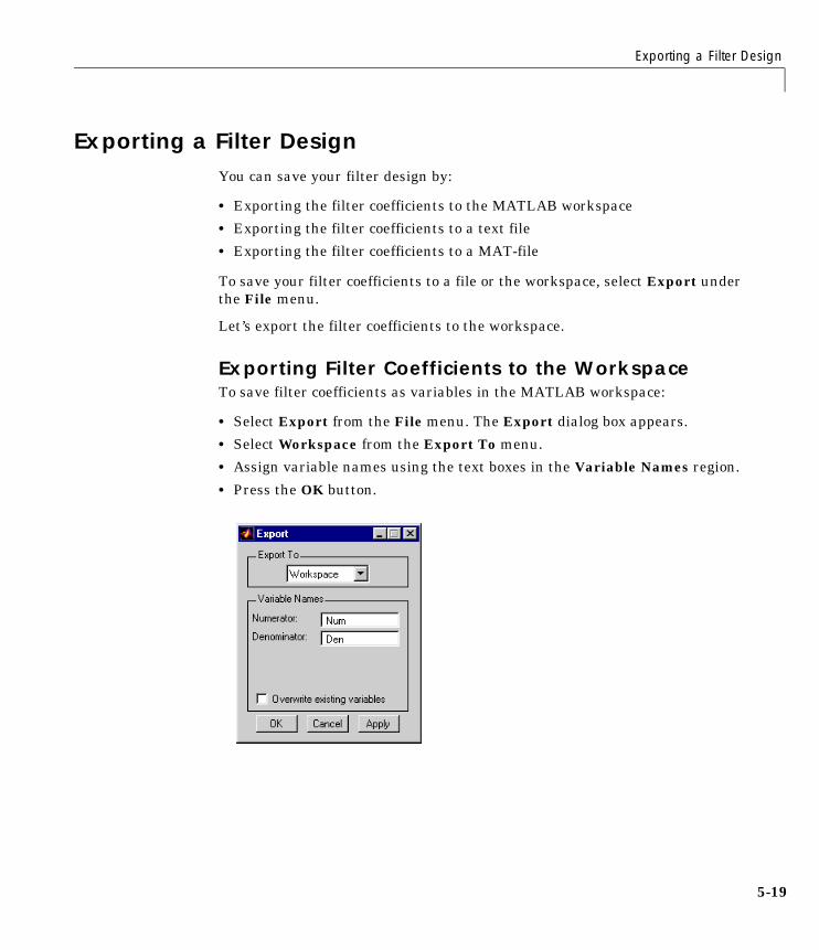
Exporting a Filter Design
5-19
Exporting a Filter DesignYou can save your filter design by:
• Exporting the filter coefficients to the MATLAB workspace
• Exporting the filter coefficients to a text file
• Exporting the filter coefficients to a MAT-file
To save your filter coefficients to a file or the workspace, select Export underthe File menu.
Let’s export the filter coefficients to the workspace.
Exporting Filter Coefficients to the WorkspaceTo save filter coefficients as variables in the MATLAB workspace:
• Select Export from the File menu. The Export dialog box appears.
• Select Workspace from the Export To menu.
• Assign variable names using the text boxes in the Variable Names region.
• Press the OK button.

5 Filter Design and Analysis Tool
5-20
Exporting Filter Coefficients to a Text FileTo save filter coefficients to a text file:
• Select Export from the File menu. The Export dialog box appears.
• Select Text-file from the Export To menu.
• Press the OK button. The Export Filter Coefficients to a Text-file dialogbox appears.
• Choose a filename and press Save.
The coefficients are saved in the text file that you specified, and the MATLABEditor opens to display the file.
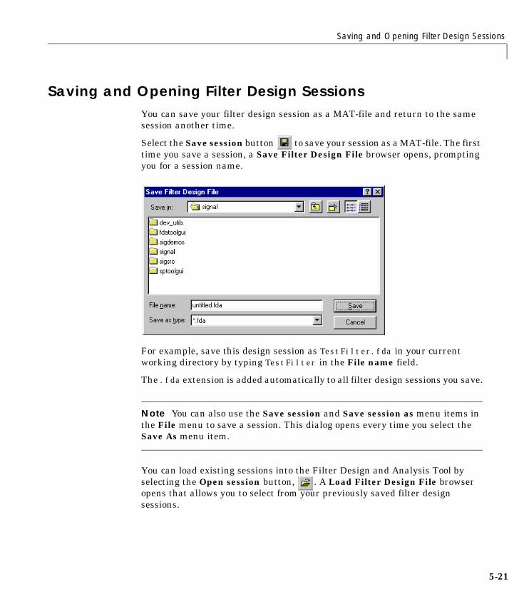
Saving and Opening Filter Design Sessions
5-21
Saving and Opening Filter Design SessionsYou can save your filter design session as a MAT-file and return to the samesession another time.
Select the Save session button to save your session as a MAT-file. The firsttime you save a session, a Save Filter Design File browser opens, promptingyou for a session name.
For example, save this design session as TestFilter.fda in your currentworking directory by typing TestFilter in the File name field.
The .fda extension is added automatically to all filter design sessions you save.
Note You can also use the Save session and Save session as menu items inthe File menu to save a session. This dialog opens every time you select theSave As menu item.
You can load existing sessions into the Filter Design and Analysis Tool byselecting the Open session button, . A Load Filter Design File browseropens that allows you to select from your previously saved filter designsessions.

5 Filter Design and Analysis Tool
5-22
6SPTool: A SignalProcessing GUI Suite
Overview . . . . . . . . . . . . . . . . . . . . . 6-2
SPTool: An Interactive Signal Processing Environment 6-3
Opening SPTool . . . . . . . . . . . . . . . . . . 6-5
Overview of the Signal Browser: Signal Analysis . . . 6-6
Overview of the Filter Designer: Filter Design . . . . 6-8
Overview of the Filter Viewer: Filter Analysis . . . . 6-11
Overview of the Spectrum Viewer: Spectral Analysis . 6-14
Getting Help . . . . . . . . . . . . . . . . . . . . 6-17
Using SPTool: Filtering and Analysis of Noise . . . . . 6-18
Importing a Signal into SPTool . . . . . . . . . . . 6-19
Designing a Filter . . . . . . . . . . . . . . . . . 6-22
Applying a Filter to a Signal . . . . . . . . . . . . . 6-24
Analyzing Signals: Opening the Signal Browser . . . . 6-26
Spectral Analysis in the Spectrum Viewer . . . . . . 6-29
Exporting Signals, Filters, and Spectra . . . . . . . . 6-32
Designing a Filter with the Pole/Zero Editor . . . . . 6-34
Redesigning a Filter Using the Magnitude Plot . . . . 6-37

6 SPTool: A Signal Processing GUI Suite
6-2
OverviewSPTool is a graphical user interface (GUI) for analyzing and manipulatingdigital signals, filters, and spectra. The first few sections of this chapter givean overview of SPTool and its associated GUIs:
• “SPTool: An Interactive Signal Processing Environment”
• “Opening SPTool”
• “Overview of the Signal Browser: Signal Analysis”
• “Overview of the Filter Designer: Filter Design”
• “Overview of the Filter Viewer: Filter Analysis”
• “Overview of the Spectrum Viewer: Spectral Analysis”
• “Getting Help”
The rest of this chapter illustrates in detail how to use the GUI-basedinteractive tools by walking through some examples:
• “Using SPTool: Filtering and Analysis of Noise”
• “Importing a Signal into SPTool”
• “Designing a Filter”
• “Applying a Filter to a Signal”
• “Analyzing Signals: Opening the Signal Browser”
• “Spectral Analysis in the Spectrum Viewer”
• “Exporting Signals, Filters, and Spectra”
• “Designing a Filter with the Pole/Zero Editor”
• “Redesigning a Filter Using the Magnitude Plot”
• “Accessing Filter Parameters in a Saved Filter”
• “Accessing Parameters in a Saved Spectrum”
• “Importing Filters and Spectra into SPTool”
• “Loading Variables from the Disk”
• “Selecting Signals, Filters, and Spectra in SPTool”
• “Editing Signals, Filters, or Spectra in SPTool”
• “Setting Preferences”
• “Making Signal Measurements: Using Markers”

SPTool: An Interactive Signal Processing Environment
6-3
SPTool: An Interactive Signal Processing EnvironmentSPTool is an interactive GUI for digital signal processing that can be used to:
• Analyze signals.
• Design filters.
• Analyze (view) filters.
• Filter signals.
• Analyze signal spectra.
You can accomplish these tasks using four GUIs that you access from withinSPTool:
• The Signal Browser is for analyzing signals. You can also play portions ofsignals using your computer’s audio hardware.
• The Filter Designer is for designing or editing the following types of FIR andIIR digital filters:
- Lowpass
- Highpass
- Bandpass
- Bandstop
Most of the Signal Processing Toolbox filter design methods available at thecommand line are also available in the Filter Designer. Additionally, you candesign a filter by using the Pole-Zero Editor to graphically place poles andzeros on the z-plane.
• The Filter Viewer is for analyzing filter characteristics. You can analyze afilter’s:
- Magnitude response
- Phase response
- Group delay
- Pole/zero plot
- Impulse response
- Step response

6 SPTool: A Signal Processing GUI Suite
6-4
• The Spectrum Viewer is for spectral analysis. You can use the SignalProcessing Toolbox spectral estimation methods to estimate the powerspectral density of a signal.
SPTool Data StructuresYou can use SPTool to analyze signals, filters, or spectra that you create at theMATLAB command line.
You can bring signals, filters, or spectra from the MATLAB workspace into theSPTool workspace using the Import item under the File menu. Signals, filters,or spectra that you create in (or import into) the SPTool workspace exist asMATLAB structures. See the MATLAB documentation for more information onMATLAB structures.
When you use the Export item under the File menu to save signals, filters, andspectra that you create or modify in SPTool, these are also saved as MATLABstructures.
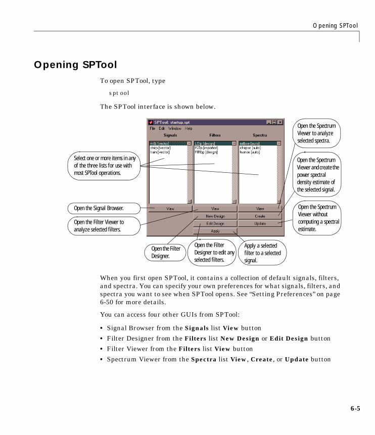
Opening SPTool
6-5
Opening SPToolTo open SPTool, type
sptool
The SPTool interface is shown below.
When you first open SPTool, it contains a collection of default signals, filters,and spectra. You can specify your own preferences for what signals, filters, andspectra you want to see when SPTool opens. See “Setting Preferences” on page6-50 for more details.
You can access four other GUIs from SPTool:
• Signal Browser from the Signals list View button
• Filter Designer from the Filters list New Design or Edit Design button
• Filter Viewer from the Filters list View button
• Spectrum Viewer from the Spectra list View, Create, or Update button
Open the Filter Viewer to analyze selected filters.
Open the Filter Designer.
Apply a selected filter to a selected signal.
Open the Spectrum Viewer to analyze selected spectra.
Open the Spectrum Viewer without computing a spectral estimate.
Select one or more items in any of the three lists for use with most SPTool operations.
Open the Signal Browser.
Open the Spectrum Viewer and create the power spectral density estimate of the selected signal.
Open the Filter Designer to edit any selected filters.
6 SPTool: A Signal Processing GUI Suite
6-6
Overview of the Signal Browser: Signal AnalysisYou can use the Signal Browser to display and analyze signals listed in theSignals list box in SPTool.
Using the Signal Browser you can:
• Analyze and compare vector or array (matrix) signals.
• Zoom in on portions of signal data.
• Measure a variety of characteristics of signal data.
• Compare multiple signals.
• Play portions of signal data on audio hardware.
• Print signal plots.
Opening the Signal BrowserYou can open the Signal Browser from SPTool by:
1 Selecting one or more signals in the Signals list in SPTool
2 Pressing the View button under the Signals list
The Signal Browser has the following components:
• A display region for analyzing signals, including markers for measuring,comparing, or playing signals
• A toolbar providing convenient access to frequently used functions:
- Zoom buttons for getting a closer look at signal features
- A button for printing signal plots
- A button for playing portions of a selected signal through audio equipment
• A “panner” that displays the entire signal length, highlighting the portioncurrently active in the display region

Overview of the Signal Browser: Signal Analysis
6-7
Toggle markers on or off
Marker measurements
Panner
Display region
Context-sensitive help
Play button for audio signals
Signal Display buttons
Print button
Choose the display color and line style of a selected signal.
Select one of several loaded signals.
Zoom buttons
6 SPTool: A Signal Processing GUI Suite
6-8
Overview of the Filter Designer: Filter DesignThe Filter Designer provides an interactive graphical environment for thedesign of digital IIR and FIR filters based on specifications that you enter on amagnitude or pole-zero plot.
Note You can also use the Filter Design and Analysis Tool (FDATool)described in Chapter 5, “Filter Design and Analysis Tool,” for filter design andanalysis.
Filter TypesYou can design filters of the following types using the Filter Designer:
• Bandpass
• Lowpass
• Bandstop
• Highpass
FIR Filter Methods You can use the following filter methods to design FIR filters:
• Equiripple
• Least squares
• Window
IIR Filter MethodsYou can use the following filter methods to design IIR filters:
• Butterworth
• Chebyshev type I
• Chebyshev type II
• Elliptic
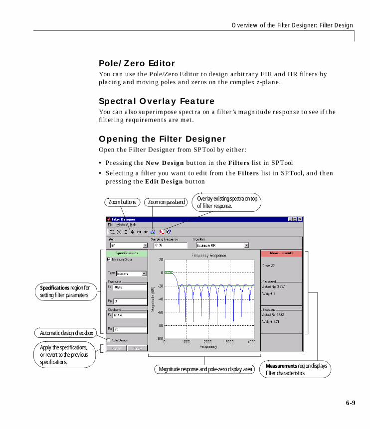
Overview of the Filter Designer: Filter Design
6-9
Pole/Zero EditorYou can use the Pole/Zero Editor to design arbitrary FIR and IIR filters byplacing and moving poles and zeros on the complex z-plane.
Spectral Overlay FeatureYou can also superimpose spectra on a filter’s magnitude response to see if thefiltering requirements are met.
Opening the Filter DesignerOpen the Filter Designer from SPTool by either:
• Pressing the New Design button in the Filters list in SPTool
• Selecting a filter you want to edit from the Filters list in SPTool, and thenpressing the Edit Design button
Automatic design checkbox
Zoom buttons
Specifications region for setting filter parameters
Magnitude response and pole-zero display area Measurements region displays filter characteristics
Apply the specifications, or revert to the previous specifications.
Zoom on passband Overlay existing spectra on top of filter response.

6 SPTool: A Signal Processing GUI Suite
6-10
The Filter Designer has the following components:
• A menu for selecting filters from the list in SPTool
• A menu for selecting different filter design methods (algorithms)
• A plot display region for graphically adjusting filter magnitude responses
• Measurement lines for measuring the magnitude response parameters of afilter
• A pole-zero plot display region for graphically editing filter designs bymanipulating transfer function poles and zeros
• Zoom buttons for navigating the displays
• A Specifications region for viewing and modifying the design parameters orpole-zero locations of the current filter
• A Measurements region for viewing the response characteristics andstability of the current filter
Overview of the Filter Viewer: Filter Analysis
6-11
Overview of the Filter Viewer: Filter AnalysisYou can use the Filter Viewer to analyze the following response characteristicsof selected filters:
• Magnitude response
• Phase response
• Impulse response
• Step response
• Group delay
• Pole and zero locations
The Filter Viewer can display up to six different response characteristics plotsfor a selected filter at any time. The Filter Viewer provides features for:
• Zooming
• Measuring filter responses
• Overlaying filter responses
• Modifying display parameters such as frequency ranges or magnitude units
Opening the Filter ViewerYou can open the Filter Viewer from SPTool by:
1 Selecting one or more filters in the Filters list in SPTool
2 Pressing the View button under the Filters list
When you first open the Filter Viewer, it displays the default plot configurationfor the selected filter(s).
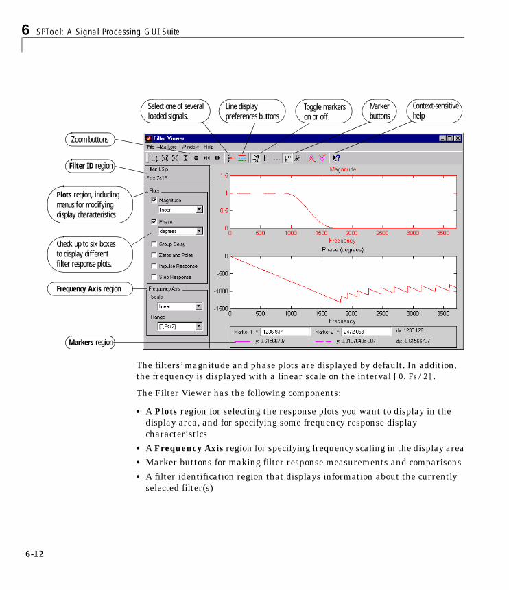
6 SPTool: A Signal Processing GUI Suite
6-12
The filters’ magnitude and phase plots are displayed by default. In addition,the frequency is displayed with a linear scale on the interval [0,Fs/2].
The Filter Viewer has the following components:
• A Plots region for selecting the response plots you want to display in thedisplay area, and for specifying some frequency response displaycharacteristics
• A Frequency Axis region for specifying frequency scaling in the display area
• Marker buttons for making filter response measurements and comparisons
• A filter identification region that displays information about the currentlyselected filter(s)
Context-sensitive help
Plots region, including menus for modifying display characteristics
Frequency Axis region
Filter ID region
Markers region
Marker buttons
Zoom buttons
Line display preferences buttons
Check up to six boxes to display different filter response plots.
Toggle markers on or off.
Select one of several loaded signals.

Overview of the Filter Viewer: Filter Analysis
6-13
• A display area for analyzing one or more frequency response plots for theselected filter(s)
• Zoom buttons to navigate the displays

6 SPTool: A Signal Processing GUI Suite
6-14
Overview of the Spectrum Viewer: Spectral AnalysisYou can use the Spectrum Viewer for estimating and analyzing a signal’spower spectral density (PSD). You can use the PSD estimates to understand asignal’s frequency content.
Using the Spectrum Viewer you can:
• Analyze and compare spectral density plots.
• Use different spectral estimation methods to create spectra:
- Burg (pburg)
- Covariance (pcov)
- FFT (fft)
- Modified covariance (pmcov)
- MTM (multitaper method) (pmtm)
- MUSIC (pmusic)
- Welch (pwelch)
- Yule-Walker AR (pyulear)
• Modify power spectral density parameters such as FFT length, window type,and sample frequency.
• Print spectral plots.
Opening the Spectrum ViewerTo open the Spectrum Viewer and create a PSD estimate from SPTool:
1 Select a signal from the Signal list box in SPTool.
2 Press the Create button in the Spectra list.
3 Press the Apply button in the Spectrum Viewer.
To open the Spectrum Viewer with a PSD estimate already listed in SPTool:
1 Select a PSD estimate from the Spectra list box in SPTool.
2 Press the View button in the Spectra list.
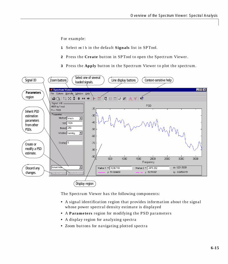
Overview of the Spectrum Viewer: Spectral Analysis
6-15
For example:
1 Select mtlb in the default Signals list in SPTool.
2 Press the Create button in SPTool to open the Spectrum Viewer.
3 Press the Apply button in the Spectrum Viewer to plot the spectrum.
The Spectrum Viewer has the following components:
• A signal identification region that provides information about the signalwhose power spectral density estimate is displayed
• A Parameters region for modifying the PSD parameters
• A display region for analyzing spectra
• Zoom buttons for navigating plotted spectra
Display region
Signal ID Zoom buttons
Parameters region
Line display buttons Context-sensitive help
Inherit PSD estimation parameters from other PSDs.
Discard any changes.
Create or modify a PSD estimate.
Select one of several loaded signals.

6 SPTool: A Signal Processing GUI Suite
6-16
• Marker buttons and line-display buttons for making spectral measurementsand comparisons
• Spectrum management controls:
- Inherit from menu to inherit PSD specifications from another PSD objectlisted in the menu
- Revert button to revert to the named PSD’s original specifications- Apply button for creating or updating PSD estimates
• Menu options for modifying plot display characteristics
• Menu options and buttons for printing PSD plots

Getting Help
6-17
Getting HelpUse the What’s this? button to find out more information about a particularregion of the GUI.
Context-Sensitive Help: The What’s This? ButtonTo find information on a particular region of the Signal Browser, FilterDesigner, Filter Viewer, or Spectrum Viewer:
1 Press the What’s this? button, .
2 Click on the region of the GUI you want information on.
You can also use the What’s this? menu item in the Help menu to launchcontext-sensitive help.
6 SPTool: A Signal Processing GUI Suite
6-18
Using SPTool: Filtering and Analysis of NoiseThe following sections provide an example of using the GUI-based interactivetools to:
• Design and implement an FIR bandpass digital filter.
• Apply the filter to a noisy signal.
• Analyze signals and their spectra.
The steps include:
• Creating a noisy signal in the MATLAB workspace and importing it intoSPTool
• Designing a bandpass filter using the Filter Designer
• Applying the filter to the original noise signal to create a bandlimited noisesignal
• Comparing the time domain information of the original and filtered signalsusing the Signal Browser
• Comparing the spectra of both signals using the Spectrum Viewer
• Exporting the filter design to the MATLAB workspace as a structure
• Accessing the filter coefficients from the exported MATLAB structure
Using SPTool: Filtering and Analysis of Noise
6-19
Importing a Signal into SPToolTo import a signal into SPTool from the workspace or disk, the signal must beeither:
• A special MATLAB signal structure, such as that saved from a previousSPTool session
• A signal created as a variable (vector or matrix) in the MATLAB workspace
For this example, create a new signal at the command line and then import itas a structure into SPTool.
1 Create a random signal in the MATLAB workspace by typing
randn('state',0);x = randn(5000,1);
2 If SPTool is not already open, open SPTool by typing
sptool
The SPTool window is displayed.
3 Select Import from the File menu in SPTool. The Import to SPTool dialogopens.

6 SPTool: A Signal Processing GUI Suite
6-20
Notice that the variable x is displayed in the Workspace Contents list. (Ifit is not, select the From Workspace radio button to display the contents ofthe workspace.)
4 Select the signal and import it into the Data field:
a Make sure that Signal is selected in the Import As pull-down menu.
b Select the signal variable x in the Workspace Contents list.
c Click on the arrow to the left of the Data field or type x in the Data field.
d Type 5000 in the Sampling Frequency field.
e Name the signal by typing noise in the Name field.
f Press OK.
At this point, the signal noise[vector] is selected in SPTool’s Signals list.
Select From Workspace to display all MATLAB workspace variables
Select From Disk to load the contents of a MAT-file into the File Contents list.
Workspace Contents (or File Contents) list
Import signals, filters, or spectra
SPTool structures appear in square brackets. Vectors and matrices are not in brackets.
Move selected items from the Workspace Contents or File Contents list to the Data field.
Edit the sampling frequency.
Edit the signal name.

Using SPTool: Filtering and Analysis of Noise
6-21
Note You can import filters and spectra into SPTool in much the same way asyou import signals. See “Importing Filters and Spectra into SPTool” on page6-43 for specific details.
You can also import signals from MAT-files on your disk, rather than from theworkspace. See “Loading Variables from the Disk” on page 6-47 for moreinformation.
Type help sptool for information about importing from the command line.

6 SPTool: A Signal Processing GUI Suite
6-22
Designing a FilterYou can import an existing filter into SPTool, or you can design and edit a newfilter using the Filter Designer.
In this example:
1 Open a default filter in the Filter Designer.
2 Specify an equiripple bandpass FIR filter.
Opening the Filter DesignerTo open the Filter Designer, press the New Design button in SPTool. Thisopens the Filter Designer with a default filter named filt1.
Specifying the Bandpass FilterDesign an equiripple bandpass FIR filter with the following characteristics:
• Sampling frequency of 5000 Hz
• Stopband frequency ranges of [0 500] Hz and [1500 2500] Hz
• Passband frequency range of [750 1250] Hz
• Ripple in the passband of 0.01 dB
• Stopband attenuation of 75 dB
To modify your filter in the Filter Designer to meet these specifications:
1 Change the filter sampling frequency to 5000 by entering this value in theSampling Frequency text box.
2 Select Equiripple FIR from the Algorithm list.
3 Select bandpass from the Type list.
4 Set the passband edge frequencies by entering 750 for Fp1 and 1250 for Fp2.
5 Set the stopband edge frequencies by entering 500 for Fs1 and 1500 for Fs2.
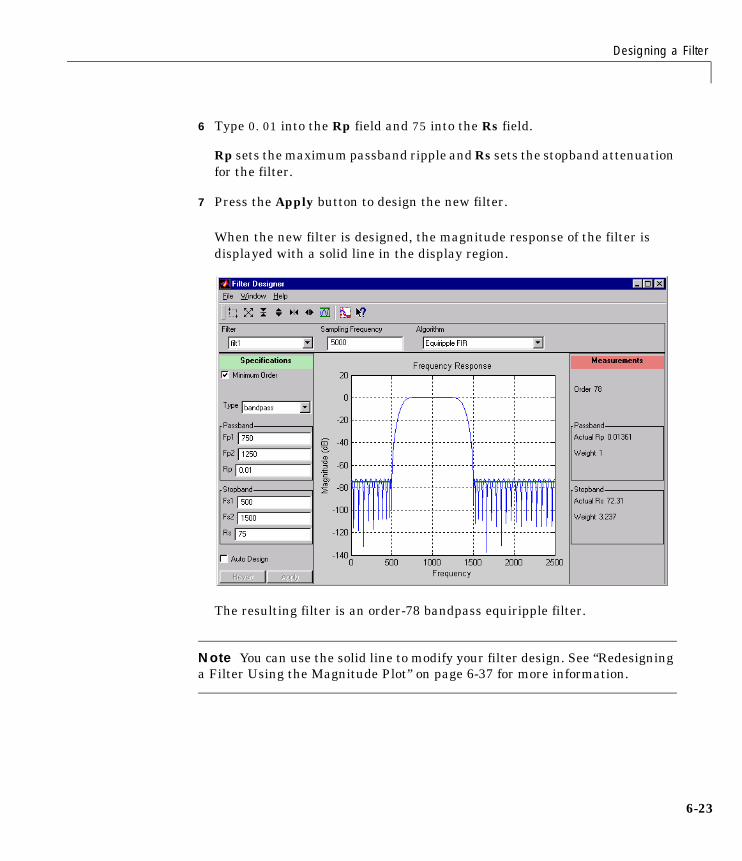
Designing a Filter
6-23
6 Type 0.01 into the Rp field and 75 into the Rs field.
Rp sets the maximum passband ripple and Rs sets the stopband attenuationfor the filter.
7 Press the Apply button to design the new filter.
When the new filter is designed, the magnitude response of the filter isdisplayed with a solid line in the display region.
The resulting filter is an order-78 bandpass equiripple filter.
Note You can use the solid line to modify your filter design. See “Redesigninga Filter Using the Magnitude Plot” on page 6-37 for more information.

6 SPTool: A Signal Processing GUI Suite
6-24
Applying a Filter to a SignalWhen you apply a filter to a signal, you create a new signal in SPToolrepresenting the filtered signal.
To apply the filter filt1 you just created to the signal noise:
1 Select SPTool from the Window menu in the Filter Designer.
2 Select the signal noise[vector] from the Signals list and select the filter(named filt1[design]) from the Filters list, as shown below.
3 Press Apply to apply the filter filt1 to the signal noise.
The Apply Filter dialog box is displayed.
The Algorithm list provides a choice of several filter structures.
Type a new signal name here.

Applying a Filter to a Signal
6-25
4 Keep the default filter structure selected in the Algorithm list. Name thenew signal by typing blnoise in the Output Signal field in this dialog box.
5 Press OK to close the Apply Filter dialog box.
The filter is applied to the selected signal and the filtered signalblnoise[vector] is listed in the Signals list in SPTool.

6 SPTool: A Signal Processing GUI Suite
6-26
Analyzing Signals: Opening the Signal BrowserYou can analyze and print signals using the Signal Browser. You can also playthe signals if your computer has audio output capabilities.
For example, compare the signal noise to the filtered signal blnoise:
1 Shift+click on the noise and blnoise signals in the Signals list of SPTool toselect both signals.
2 Press the View button under the Signals list.
The Signal Browser is activated and both signals are displayed in thedisplay region. (The names of both signals are shown above the displayregion.) Initially, the original noise signal covers up the bandlimitedblnoise signal.
3 Push the selection button on the toolbar, , to select the blnoise signal.
The display area is updated. Now you can see the blnoise signalsuperimposed on top of the noise signal. The signals are displayed indifferent colors in both the display region and the panner. You can changethe color of the selected signal using the Line Properties button on thetoolbar, .
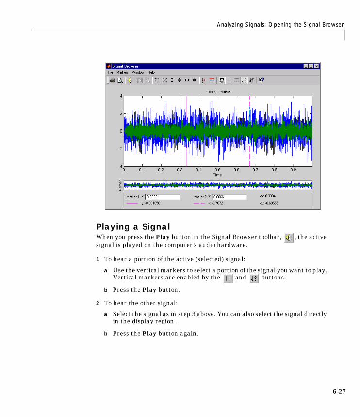
Analyzing Signals: Opening the Signal Browser
6-27
Playing a SignalWhen you press the Play button in the Signal Browser toolbar, , the activesignal is played on the computer’s audio hardware.
1 To hear a portion of the active (selected) signal:
a Use the vertical markers to select a portion of the signal you want to play.Vertical markers are enabled by the and buttons.
b Press the Play button.
2 To hear the other signal:
a Select the signal as in step 3 above. You can also select the signal directlyin the display region.
b Press the Play button again.
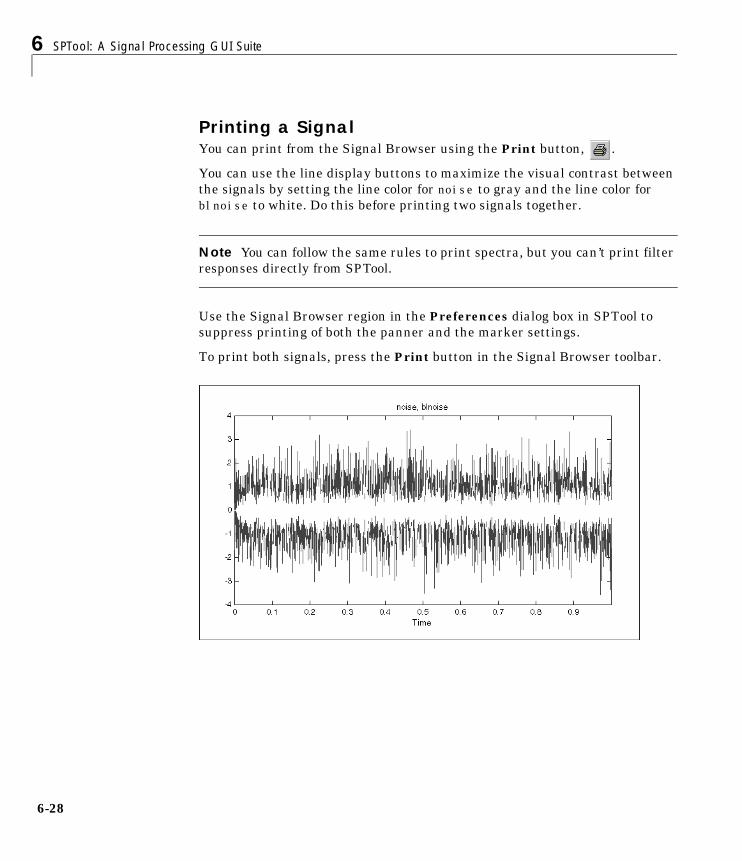
6 SPTool: A Signal Processing GUI Suite
6-28
Printing a SignalYou can print from the Signal Browser using the Print button, .
You can use the line display buttons to maximize the visual contrast betweenthe signals by setting the line color for noise to gray and the line color forblnoise to white. Do this before printing two signals together.
Note You can follow the same rules to print spectra, but you can’t print filterresponses directly from SPTool.
Use the Signal Browser region in the Preferences dialog box in SPTool tosuppress printing of both the panner and the marker settings.
To print both signals, press the Print button in the Signal Browser toolbar.

Spectral Analysis in the Spectrum Viewer
6-29
Spectral Analysis in the Spectrum ViewerYou can analyze the frequency content of a signal using the Spectrum Viewer,which estimates and displays a signal’s power spectral density.
For example, to analyze and compare the spectra of noise and blnoise:
1 Create a power spectral density object, spect1, that is associated with thesignal noise, and a second power spectral density object, spect2, that isassociated with the signal blnoise.
2 Open the Spectrum Viewer to analyze both of these spectra.
3 Print both spectra.
Creating a PSD Object From a Signal
1 Click on SPTool, or select SPTool from the Window menu of any active openGUI. SPTool is now the active window.
2 Select the noise[vector] signal in the Signals list of SPTool.
3 Press Create in the Spectra list.
The Spectrum Viewer is activated, and a power spectral density object(spect1) corresponding to the noise signal is created in the Spectra list.The power spectral density is not computed or displayed yet.
4 Press Apply in the Spectrum Viewer to compute and display the powerspectral density estimate spect1 using the default parameters.
The power spectral density of the noise signal is displayed in the displayregion. The identifying information for the power spectral density’sassociated signal (noise) is displayed above the Parameters region.
The power spectral density estimate spect1 is within 2 or 3 dB of 0, so thenoise has a fairly “flat” power spectral density.
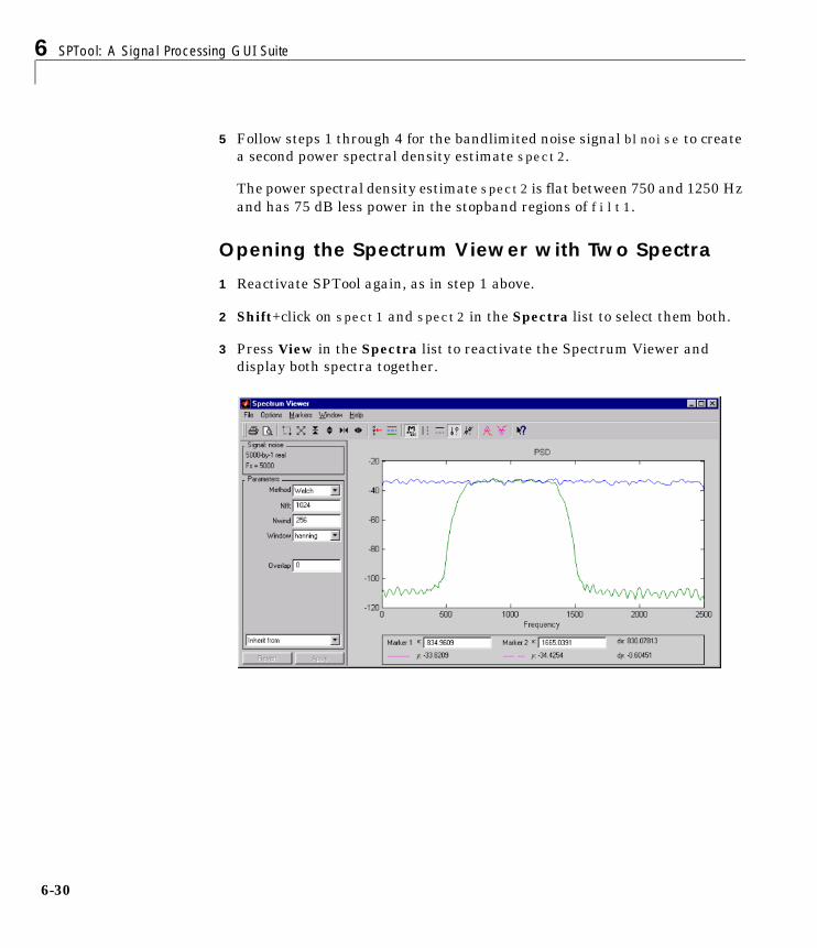
6 SPTool: A Signal Processing GUI Suite
6-30
5 Follow steps 1 through 4 for the bandlimited noise signal blnoise to createa second power spectral density estimate spect2.
The power spectral density estimate spect2 is flat between 750 and 1250 Hzand has 75 dB less power in the stopband regions of filt1.
Opening the Spectrum Viewer with Two Spectra
1 Reactivate SPTool again, as in step 1 above.
2 Shift+click on spect1 and spect2 in the Spectra list to select them both.
3 Press View in the Spectra list to reactivate the Spectrum Viewer anddisplay both spectra together.
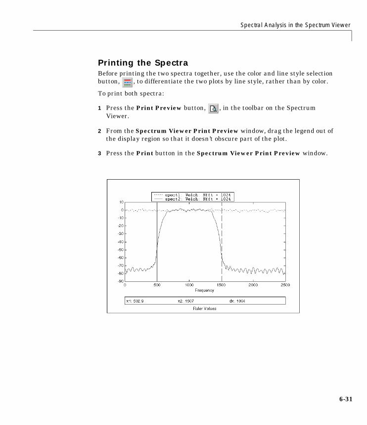
Spectral Analysis in the Spectrum Viewer
6-31
Printing the SpectraBefore printing the two spectra together, use the color and line style selectionbutton, , to differentiate the two plots by line style, rather than by color.
To print both spectra:
1 Press the Print Preview button, , in the toolbar on the SpectrumViewer.
2 From the Spectrum Viewer Print Preview window, drag the legend out ofthe display region so that it doesn’t obscure part of the plot.
3 Press the Print button in the Spectrum Viewer Print Preview window.
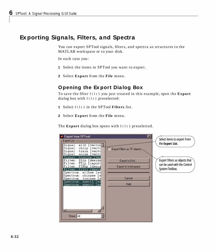
6 SPTool: A Signal Processing GUI Suite
6-32
Exporting Signals, Filters, and SpectraYou can export SPTool signals, filters, and spectra as structures to theMATLAB workspace or to your disk.
In each case you:
1 Select the items in SPTool you want to export.
2 Select Export from the File menu.
Opening the Export Dialog BoxTo save the filter filt1 you just created in this example, open the Exportdialog box with filt1 preselected:
1 Select filt1 in the SPTool Filters list.
2 Select Export from the File menu.
The Export dialog box opens with filt1 preselected.
Select items to export from the Export List.
Export filters as objects that can be used with the Control System Toolbox.

Exporting Signals, Filters, and Spectra
6-33
Exporting a Filter to the MATLAB WorkspaceTo export the filter filt1 to the MATLAB workspace:
1 Select filt1 and deselect all other items using Ctrl+click.
2 Press the Export to Workspace button.

6 SPTool: A Signal Processing GUI Suite
6-34
Designing a Filter with the Pole/Zero EditorTo design a filter transfer function using the Filter Designer’s Pole/Zero Editor:
1 Select the Pole/Zero Editor option from theAlgorithm list.
This opens the Pole/Zero Editor in the FilterDesigner display.
2 Enter the desired filter gain in the Gain edit box.
3 Select a pole or zero (or conjugate pair) by selecting one of the (pole) or(zero) symbols on the plot.
4 Choose the coordinates to work in by specifying Polar or Rectangular fromthe Coordinates list.
5 Specify the new location(s) of the selected pole, zero, or conjugate pair bytyping values into the Mag and Angle fields (for angular coordinates) or Xand Y (for rectangular coordinates) fields. Alternatively, position the polesand zeros by dragging the and symbols.
6 Use the Conjugate pair check box to create a conjugate pair from a lone poleor zero, or to break a conjugate pair into two individual poles or zeros.
Design a new filter or edit an existing filter in the same way.
Tip Keep the Filter Viewer open while designing a filter with the Pole/ZeroEditor. Any changes that you make to the filter transfer function in thePole/Zero Editor are then simultaneously reflected in the response plots of theFilter Viewer.
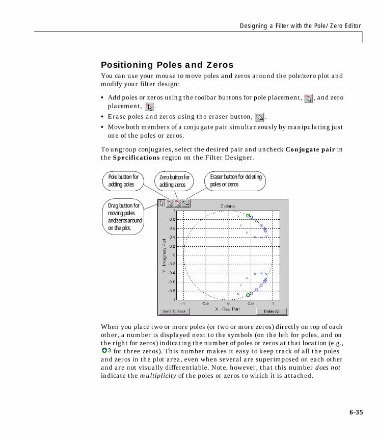
Designing a Filter with the Pole/Zero Editor
6-35
Positioning Poles and ZerosYou can use your mouse to move poles and zeros around the pole/zero plot andmodify your filter design:
• Add poles or zeros using the toolbar buttons for pole placement, , and zeroplacement, .
• Erase poles and zeros using the eraser button, .
• Move both members of a conjugate pair simultaneously by manipulating justone of the poles or zeros.
To ungroup conjugates, select the desired pair and uncheck Conjugate pair inthe Specifications region on the Filter Designer.
When you place two or more poles (or two or more zeros) directly on top of eachother, a number is displayed next to the symbols (on the left for poles, and onthe right for zeros) indicating the number of poles or zeros at that location (e.g.,
for three zeros). This number makes it easy to keep track of all the polesand zeros in the plot area, even when several are superimposed on each otherand are not visually differentiable. Note, however, that this number does notindicate the multiplicity of the poles or zeros to which it is attached.
Pole button for adding poles
Zero button for adding zeros
Eraser button for deleting poles or zeros
Drag button for moving poles and zeros around on the plot.

6 SPTool: A Signal Processing GUI Suite
6-36
To detect whether or not a set of poles or zeros are truly multiples, use the zoomtools to magnify the region around the poles or zeros in question. Becausenumerical limitations usually prevent any set of poles or zeros from sharingexactly the same value, at a high enough zoom level even truly multiple polesor zeros appear distinct from each other.
A common way to assess whether a particular group of poles or zeros containsmultiples is by comparing the mutual proximity of the group members againsta selected threshold value. As an example, the residuez function defines a poleor zero as being a multiple of another pole or zero if the absolute distanceseparating them is less than 0.1% of the larger pole or zero’s magnitude.
Redesigning a Filter Using the Magnitude Plot
6-37
Redesigning a Filter Using the Magnitude PlotAfter designing a filter in the Filter Designer, you can redesign it by draggingthe specification lines on the magnitude plot. Use the specification lines tochange passband ripple, stopband attenuation, and edge frequencies.
In the following example, create a Chebyshev filter and modify it by draggingthe specification lines:
1 Select Chebyshev Type I IIR from the Algorithm menu.
2 Select highpass from the Type menu.
3 Type 2000 in the Sampling Frequency field.
4 Set the following parameters:
a Fp = 800
b Fs = 700
c Rp = 2.5
d Rs = 35
5 Check Minimum Order so the Filter Designer can calculate the lowest filterorder that produces the desired characteristics.
6 Press Apply to compute the filter and update the response plot.
7 Position the cursor over the horizontal filter specification line for thestopband. This is the first (leftmost) horizontal specification line you see.
The cursor changes to the up/down drag indicator.
8 Drag the line until the Rs (stopband attenuation) field reads 100.
Note The Order value in the Measurements region changes because ahigher filter order is needed to meet the new specifications.
6 SPTool: A Signal Processing GUI Suite
6-38
Accessing Filter Parameters in a Saved FilterThe MATLAB structures created by SPTool have several associated fields,many of which are also MATLAB structures. See the MATLAB documentationfor general information about MATLAB structures.
For example, after exporting a filter filt1 to the MATLAB workspace, type
filt1
to display the fields of the MATLAB filter structure. The tf, Fs, and specsfields of the structure contain the information that describes the filter.
The tf Field: Accessing Filter CoefficientsThe tf field is a structure containing the transfer function representation ofthe filter. Use this field to obtain the filter coefficients:
• filt1.tf.num contains the numerator coefficients.
• filt1.tf.den contains the denominator coefficients.
The vectors contained in these structures represent polynomials in descendingpowers of z. The numerator and denominator polynomials are used to specifythe transfer function
where:
• b is a vector containing the coefficients from the tf.num field.
• a is a vector containing the coefficients from the tf.den field.
• m is the numerator order.
• n is the denominator order.
You can change the filter representation from the default transfer function toanother form by using the tf2ss or tf2zp functions.
The Fs Field: Accessing Filter Sample FrequencyThe Fs field contains the sampling frequency of the filter in hertz.
H z( )B z( )A z( )-----------
b 1( ) b 2( )z 1– b nb 1+( )z m–+ + +
a 1( ) a 2( )z 1– a na 1+( )z n–+ + +-----------------------------------------------------------------------------------------= =
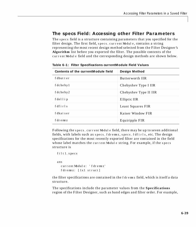
Accessing Filter Parameters in a Saved Filter
6-39
The specs Field: Accessing other Filter ParametersThe specs field is a structure containing parameters that you specified for thefilter design. The first field, specs.currentModule, contains a stringrepresenting the most recent design method selected from the Filter Designer’sAlgorithm list before you exported the filter. The possible contents of thecurrentModule field and the corresponding design methods are shown below.
Following the specs.currentModule field, there may be up to seven additionalfields, with labels such as specs.fdremez, specs.fdfirls, etc. The designspecifications for the most recently exported filter are contained in the fieldwhose label matches the currentModule string. For example, if the specsstructure is
filt1.specs
anscurrentModule: 'fdremez'fdremez: [1x1 struct]
the filter specifications are contained in the fdremez field, which is itself a datastructure.
The specifications include the parameter values from the Specificationsregion of the Filter Designer, such as band edges and filter order. For example,
Table 6-1: Filter Specifications currentModule Field Values
Contents of the currentModule field Design Method
fdbutter Butterworth IIR
fdcheby1 Chebyshev Type I IIR
fdcheby2 Chebyshev Type II IIR
fdellip Elliptic IIR
fdfirls Least Squares FIR
fdkaiser Kaiser Window FIR
fdremez Equiripple FIR

6 SPTool: A Signal Processing GUI Suite
6-40
the filter above has the following specifications stored infilt1.specs.fdremez.
filt1.specs.fdremez
ans = setOrderFlag: 0 type: 3 f: [0 0.2000 0.3000 0.5000 0.6000 1] m: [6x1 double] Rp: 0.0100 Rs: 75 wt: [3.2371 1 3.2371] order: 78
Because certain filter parameters are unique to a particular design, thisstructure has a different set of fields for each filter design.
The table below describes the possible fields associated with the filter designspecification field (the specs field) that can appear in the exported structure.
Table 6-2: SPTool Structure Specifications for Filters
Parameter Description
Beta Kaiser window β parameter.
f Contains a vector of band-edge frequencies, normalized sothat 1 Hz corresponds to half the sample frequency.
Fpass Passband cutoff frequencies. Scalar for lowpass andhighpass designs, two-element vector for bandpass andbandstop designs.
Fstop Stopband cutoff frequencies. Scalar for lowpass andhighpass designs, two-element vector for bandpass andbandstop designs.
m The response magnitudes corresponding to the band-edgefrequencies in f.
order Filter order.

Accessing Filter Parameters in a Saved Filter
6-41
Rp Passband ripple (dB)
Rs Stopband attenuation (dB)
setOrderFlag Contains 1 if the filter order was specified manually (i.e.,the Minimum Order box in the Specifications regionwas not checked). Contains 0 if the filter order wascomputed automatically.
type Contains 1 for lowpass, 2 for highpass, 3 for bandpass, or4 for bandstop.
w3db -3 dB frequency for Butterworth IIR designs.
wind Vector of Kaiser window coefficients.
Wn Cutoff frequency for the Kaiser window FIR filter whensetOrderFlag = 1.
wt Vector of weights, one weight per frequency band.
Table 6-2: SPTool Structure Specifications for Filters (Continued)
Parameter Description
6 SPTool: A Signal Processing GUI Suite
6-42
Accessing Parameters in a Saved SpectrumThe following structure fields describe the spectra saved by SPTool.
You can access the information in these fields as you do with every MATLABstructure.
For example, if you export an SPTool PSD estimate spect1 to the workspace,type
spect1.P
to obtain the vector of associated power values.
Field Description
P The spectral power vector.
f The spectral frequency vector.
confid A structure containing the confidence intervals data:
• The confid.level field contains the chosenconfidence level.
• The confid.Pc field contains the spectral powerdata for the confidence intervals.
• The confid.enable field contains a 1 if confidencelevels are enabled for the power spectral density.
signalLabel The name of the signal from which the power spectraldensity was generated.
Fs The associated signal’s sample rate.
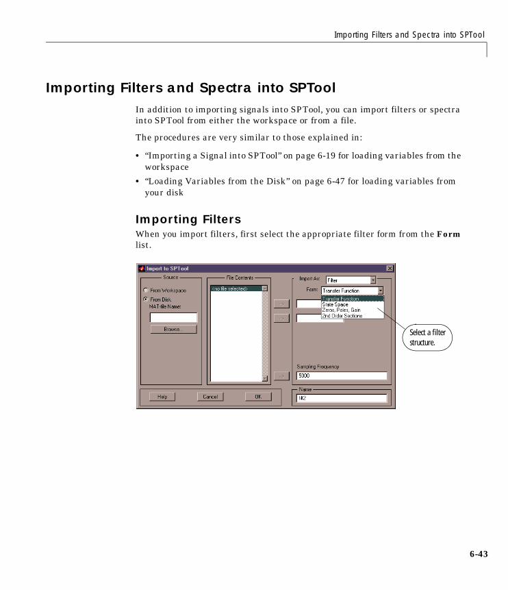
Importing Filters and Spectra into SPTool
6-43
Importing Filters and Spectra into SPToolIn addition to importing signals into SPTool, you can import filters or spectrainto SPTool from either the workspace or from a file.
The procedures are very similar to those explained in:
• “Importing a Signal into SPTool” on page 6-19 for loading variables from theworkspace
• “Loading Variables from the Disk” on page 6-47 for loading variables fromyour disk
Importing FiltersWhen you import filters, first select the appropriate filter form from the Formlist.
Select a filter structure.
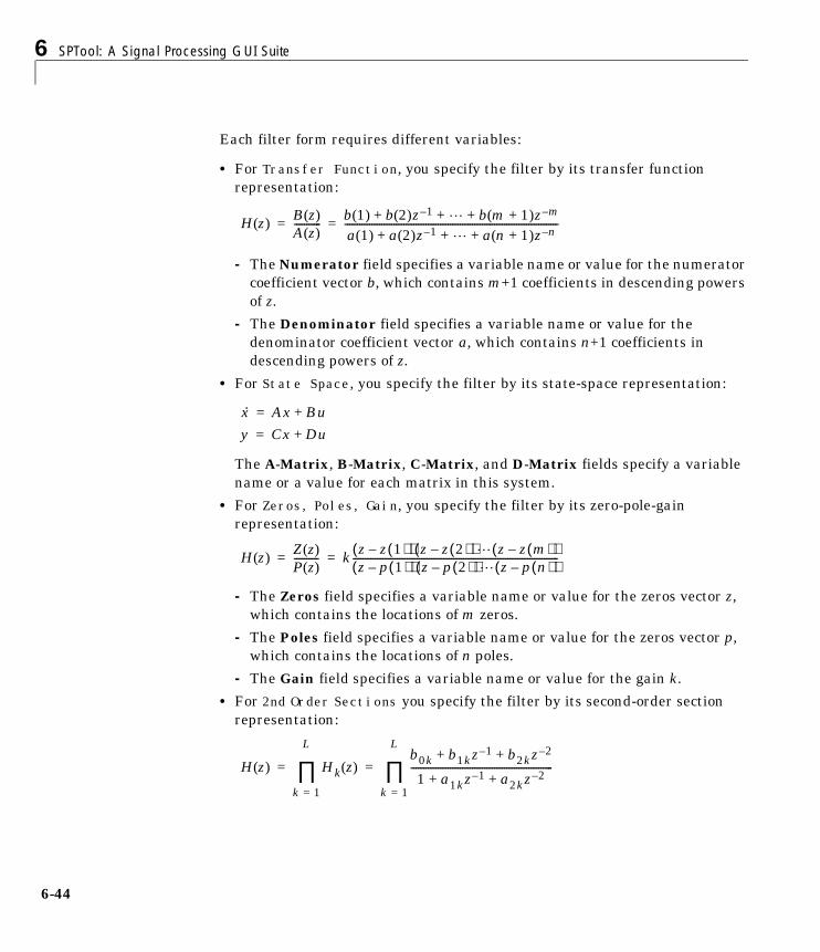
6 SPTool: A Signal Processing GUI Suite
6-44
Each filter form requires different variables:
• For Transfer Function, you specify the filter by its transfer functionrepresentation:
- The Numerator field specifies a variable name or value for the numeratorcoefficient vector b, which contains m+1 coefficients in descending powersof z.
- The Denominator field specifies a variable name or value for thedenominator coefficient vector a, which contains n+1 coefficients indescending powers of z.
• For State Space, you specify the filter by its state-space representation:
The A-Matrix, B-Matrix, C-Matrix, and D-Matrix fields specify a variablename or a value for each matrix in this system.
• For Zeros, Poles, Gain, you specify the filter by its zero-pole-gainrepresentation:
- The Zeros field specifies a variable name or value for the zeros vector z,which contains the locations of m zeros.
- The Poles field specifies a variable name or value for the zeros vector p,which contains the locations of n poles.
- The Gain field specifies a variable name or value for the gain k.
• For 2nd Order Sections you specify the filter by its second-order sectionrepresentation:
H z( )B z( )A z( )-----------
b 1( ) b 2( )z 1– b m 1+( )z m–+ + +a 1( ) a 2( )z 1– a n 1+( )z n–+ + +---------------------------------------------------------------------------------------= =
x· Ax Bu+=
y Cx Du+=
H z( )Z z( )P z( )---------- k z z 1( )–( ) z z 2( )–( ) z z m( )–( )
z p 1( )–( ) z p 2( )–( ) z p n( )–( )------------------------------------------------------------------------------------= =
H z( ) Hk z( )
k 1=
L
∏b0k b1kz 1– b2kz 2–+ +
1 a1kz 1– a2kz 2–+ +----------------------------------------------------------
k 1=
L
∏= =

Importing Filters and Spectra into SPTool
6-45
The SOS Matrix field specifies a variable name or a value for the L-by-6 SOSmatrix
whose rows contain the numerator and denominator coefficients bik and aikof the second-order sections of H(z).
• For every filter you specify a variable name or a value for the filter’ssampling frequency in the Sampling Frequency field.
Note If you import a filter that was not created in SPTool, you can only editthat filter using the Pole/Zero Editor.
Importing SpectraWhen you import a power spectral density (PSD), you specify:
• A variable name or a value for the PSD vector in the PSD field
• A variable name or a value for the frequency vector in the Freq. Vector field
sos
b01 b11 b21 1 a11 a21
b02 b12 b22 1 a12 a22
b0L b1L b2L 1 a1L a2L
=

6 SPTool: A Signal Processing GUI Suite
6-46
The PSD values in the PSD vector correspond to the frequencies containedin the Freq. Vector vector; the two vectors must have the same length.
Loading Variables from the Disk
6-47
Loading Variables from the DiskTo import variables representing signals, filters, or spectra from a MAT-file onyour disk:
1 Select the From Disk radio button and do either of the following:
- Type the name of the file you want to import into the MAT-file Name fieldand press either the Tab or the Enter key on your keyboard.
- Select Browse, and then find and select the file you want to import usingthe Select File to Open dialog. Press OK to close that dialog.
In either case, all variables in the MAT-file you selected are displayed in theFile Contents list.
2 Select the variables to be imported into SPTool.
You can now import one or more variables from the File Contents list intoSPTool, as long as these variables are scalars, vectors, or matrices.

6 SPTool: A Signal Processing GUI Suite
6-48
Selecting Signals, Filters, and Spectra in SPToolAll signals, filters, or spectra listed in SPTool exist as special MATLABstructures. You can bring data representing signals, filters, or spectra intoSPTool from the MATLAB workspace. In general, you can select one or severalitems in a given list box. An item is selected when it is highlighted.
The Signals list shows all vector and array signals in the current SPToolsession.
The Filters list shows all designed and imported filters in the current SPToolsession.
The Spectra list shows all spectra in the current SPTool session.
You can select a single data object in a list, a range of data objects in a list, ormultiple separate data objects in a list. You can also have data objectssimultaneously selected in different lists:
• To select a single item, click on it. All other items in that list box becomedeselected.
• To add or remove a range of items, Shift+click on the items at the top andbottom of the section of the list that you want to add. You can also drag yourmouse pointer to select these items.
• To add a single data object to a selection or remove a single data object froma multiple selection, Ctrl+click on the object.
Editing Signals, Filters, or Spectra in SPTool
6-49
Editing Signals, Filters, or Spectra in SPToolYou can edit selected items in SPTool by:
1 Selecting the names of the signals, filters, or spectra you want to edit.
2 Selecting the appropriate Edit menu item:
- Duplicate to copy an item in an SPTool list
- Clear to delete an item in an SPTool list
- Name to rename an item in an SPTool list
- Sampling Frequency to modify the sampling frequency associated witheither a signal (and its associated spectra) or filter in an SPTool list
The pull-down menu next to each menu item shows the names of all selecteditems.
You can also edit the following signal characteristics by right-clicking in thedisplay region of the Signal Browser, the Filter Viewer, or the SpectrumViewer:
• The signal name
• The sampling frequency
• The line style properties
Note If you modify the sampling frequency associated with a signal’sspectrum using the right-click menu on the Spectrum Viewer display region,the sampling frequency of the associated signal is automatically updated.
6 SPTool: A Signal Processing GUI Suite
6-50
Setting PreferencesUse Preferences from the SPTool File menu to customize displays and certainparameters for SPTool and its four component GUIs. The new settings aresaved on disk and are used when you restart SPTool from MATLAB.
In the Preferences regions, you can:
• Select colors and markers for all displays.
• Select colors and line styles for displayed signals.
• Configure labels, and enable/disable markers, panner, and zoom in theSignal Browser.
• Configure display parameters, and enable/disable markers and zoom in theSpectrum Viewer.
• Configure filter and display parameters, and enable/disable zoom in theFilter Viewer.
• Configure tiling preferences in the Filter Viewer.
• Specify FFT length, and enable/disable mouse zoom and grid in the FilterDesigner.
• Enable/disable use of a default session file.
• Export filters for use with the Control System Toolbox.
• Enable/disable search for plug-ins at start-up.
When you first select Preferences, the Preferences dialog box opens withMarkers selected by default. You can:
• Change the settings for markers from this panel of the Preferences dialog.
• Choose any of the other categories listed to customize its settings.
Click once on any listed category in the left pane of the Preferences dialog toselect it.

Making Signal Measurements: Using Markers
6-51
Making Signal Measurements: Using MarkersYou can use the markers on the Signal Browser, the Filter Viewer, or theSpectrum Viewer to make measurements on any of the following:
• A signal in the Signal Browser
• A filter response in the Filter Viewer
• A power spectral density plotted in the Spectrum Viewer
To make a measurement:
1 Select a line to measure (or play, if you are in the Signal Browser).
2 Select one of the marker buttons, , , , , , , to apply amarker to the displayed signal.
3 Position a marker in the main display area by grabbing it with your mouseand dragging:
a Select a marker setting. If you choose the Vertical, Track, or Slopebuttons, you can drag a marker to the right or left. If you choose theHorizontal button, you can drag a marker up or down.
b Move the mouse over the marker (1 or 2) that you want to drag.
The hand cursor with the marker number inside it is displayed whenyour mouse passes over a marker.
c Drag the marker to where you want it on the signal.
As you drag a marker, the bottom of the Signal Browser shows the currentposition of both markers. Depending on which marker setting you select,some or all of the following fields are displayed: x1, y1, x2, y2, dx, dy, m.These fields are also displayed when you print from the Signal Browser,unless you suppress them.
You can also position a marker by typing its x1 and x2 or y1 and y2 values inthe region at the bottom.

6 SPTool: A Signal Processing GUI Suite
6-52
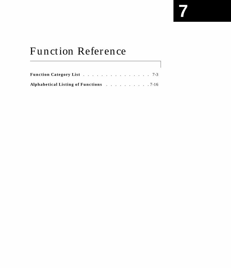
7
Function Reference
Function Category List . . . . . . . . . . . . . . . 7-3
Alphabetical Listing of Functions . . . . . . . . . . 7-16

7 Function Reference
7-2
This chapter contains detailed descriptions of all Signal Processing Toolboxfunctions. It is divided into two sections:
• “Function Category List” – a list of functions, grouped by subject area
• “Alphabetical List of Functions” – reference pages in alphabetical order

Function Category List
7-3
Function Category ListThe tables below list all of the Signal Processing Toolbox functions by category.
Filter Analysis
abs Absolute value (magnitude).
angle Phase angle.
freqs Frequency response of analog filters.
freqspace Frequency spacing for frequency response.
freqz Compute the frequency response of digital filters.
freqzplot Plot frequency response data.
grpdelay Compute the average filter delay (group delay).
impz Compute the impulse response of digital filters.
unwrap Unwrap phase angles.
zplane Zero-pole plot.
Filter Implementation
conv Convolution and polynomial multiplication.
conv2 Two-dimensional convolution.
deconv Deconvolution and polynomial division.
fftfilt FFT-based FIR filtering using the overlap-add method.
filter Filter data with a recursive (IIR) or nonrecursive (FIR)filter.
filter2 Two-dimensional digital filtering.
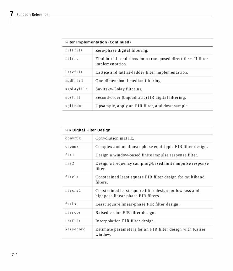
7 Function Reference
7-4
filtfilt Zero-phase digital filtering.
filtic Find initial conditions for a transposed direct form II filterimplementation.
latcfilt Lattice and lattice-ladder filter implementation.
medfilt1 One-dimensional median filtering.
sgolayfilt Savitzky-Golay filtering.
sosfilt Second-order (biquadratic) IIR digital filtering.
upfirdn Upsample, apply an FIR filter, and downsample.
FIR Digital Filter Design
convmtx Convolution matrix.
cremez Complex and nonlinear-phase equiripple FIR filter design.
fir1 Design a window-based finite impulse response filter.
fir2 Design a frequency sampling-based finite impulse responsefilter.
fircls Constrained least square FIR filter design for multibandfilters.
fircls1 Constrained least square filter design for lowpass andhighpass linear phase FIR filters.
firls Least square linear-phase FIR filter design.
firrcos Raised cosine FIR filter design.
intfilt Interpolation FIR filter design.
kaiserord Estimate parameters for an FIR filter design with Kaiserwindow.
Filter Implementation (Continued)

Function Category List
7-5
remez Compute the Parks-McClellan optimal FIR filter design.
remezord Parks-McClellan optimal FIR filter order estimation.
sgolay Savitzky-Golay filter design.
IIR Digital Filter Design—Classical and Direct
butter Butterworth analog and digital filter design.
cheby1 Chebyshev type I filter design (passband ripple).
cheby2 Chebyshev type II filter design (stopband ripple).
ellip Elliptic (Cauer) filter design.
maxflat Generalized digital Butterworth filter design.
prony Prony’s method for time-domain IIR filter design.
stmcb Compute a linear model using Steiglitz-McBride iteration.
yulewalk Recursive digital filter design.
IIR Filter Order Estimation
buttord Calculate the order and cutoff frequency for a Butterworthfilter.
cheb1ord Calculate the order for a Chebyshev type I filter.
cheb2ord Calculate the order for a Chebyshev type II filter.
ellipord Calculate the minimum order for elliptic filters.
FIR Digital Filter Design (Continued)
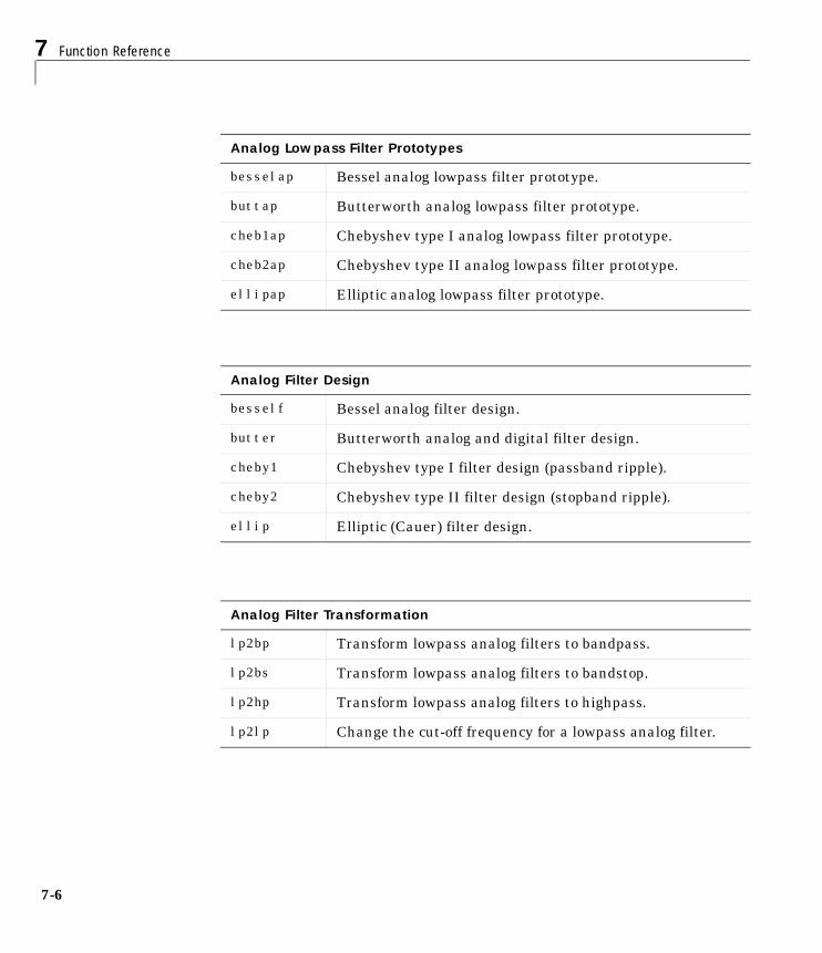
7 Function Reference
7-6
Analog Lowpass Filter Prototypes
besselap Bessel analog lowpass filter prototype.
buttap Butterworth analog lowpass filter prototype.
cheb1ap Chebyshev type I analog lowpass filter prototype.
cheb2ap Chebyshev type II analog lowpass filter prototype.
ellipap Elliptic analog lowpass filter prototype.
Analog Filter Design
besself Bessel analog filter design.
butter Butterworth analog and digital filter design.
cheby1 Chebyshev type I filter design (passband ripple).
cheby2 Chebyshev type II filter design (stopband ripple).
ellip Elliptic (Cauer) filter design.
Analog Filter Transformation
lp2bp Transform lowpass analog filters to bandpass.
lp2bs Transform lowpass analog filters to bandstop.
lp2hp Transform lowpass analog filters to highpass.
lp2lp Change the cut-off frequency for a lowpass analog filter.

Function Category List
7-7
Filter Discretization
bilinear Bilinear transformation method for analog-to-digital filterconversion.
impinvar Impulse invariance method for analog-to-digital filterconversion.
Linear System Transformations
latc2tf Convert lattice filter parameters to transfer function form.
polystab Stabilize a polynomial.
polyscale Scale the roots of a polynomial.
residuez z-transform partial-fraction expansion.
sos2ss Convert digital filter second-order section parameters tostate-space form.
sos2tf Convert digital filter second-order section data to transferfunction form.
sos2zp Convert digital filter second-order sections parameters tozero-pole-gain form.
ss2sos Convert digital filter state-space parameters tosecond-order sections form.
ss2tf Convert state-space filter parameters to transfer functionform.
ss2zp Convert state-space filter parameters to zero-pole-gainform.
tf2latc Convert transfer function filter parameters to lattice filterform.
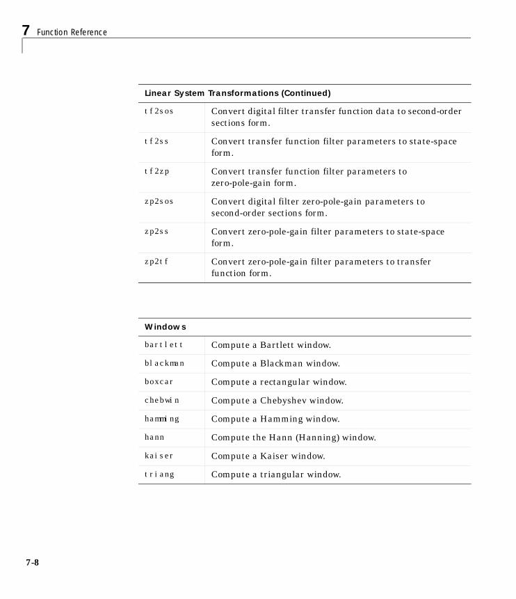
7 Function Reference
7-8
tf2sos Convert digital filter transfer function data to second-ordersections form.
tf2ss Convert transfer function filter parameters to state-spaceform.
tf2zp Convert transfer function filter parameters tozero-pole-gain form.
zp2sos Convert digital filter zero-pole-gain parameters tosecond-order sections form.
zp2ss Convert zero-pole-gain filter parameters to state-spaceform.
zp2tf Convert zero-pole-gain filter parameters to transferfunction form.
Windows
bartlett Compute a Bartlett window.
blackman Compute a Blackman window.
boxcar Compute a rectangular window.
chebwin Compute a Chebyshev window.
hamming Compute a Hamming window.
hann Compute the Hann (Hanning) window.
kaiser Compute a Kaiser window.
triang Compute a triangular window.
Linear System Transformations (Continued)

Function Category List
7-9
Transforms
czt Chirp z-transform.
dct Discrete cosine transform (DCT).
dftmtx Discrete Fourier transform matrix.
fft Compute the one-dimensional fast Fourier transform.
fft2 Compute the two-dimensional fast Fourier transform.
fftshift Rearrange the outputs of the FFT functions.
hilbert Compute the discrete-time analytic signal using the Hilberttransform.
idct Inverse discrete cosine transform.
ifft One-dimensional inverse fast Fourier transform.
ifft2 Two-dimensional inverse fast Fourier transform.
Cepstral Analysis
cceps Complex cepstral analysis.
icceps Inverse complex cepstrum.
rceps Real cepstrum and minimum phase reconstruction.
Statistical Signal Processing and Spectral Analysis
cohere Estimate magnitude squared coherence function betweentwo signals.
corrcoef Compute the correlation coefficient matrix.
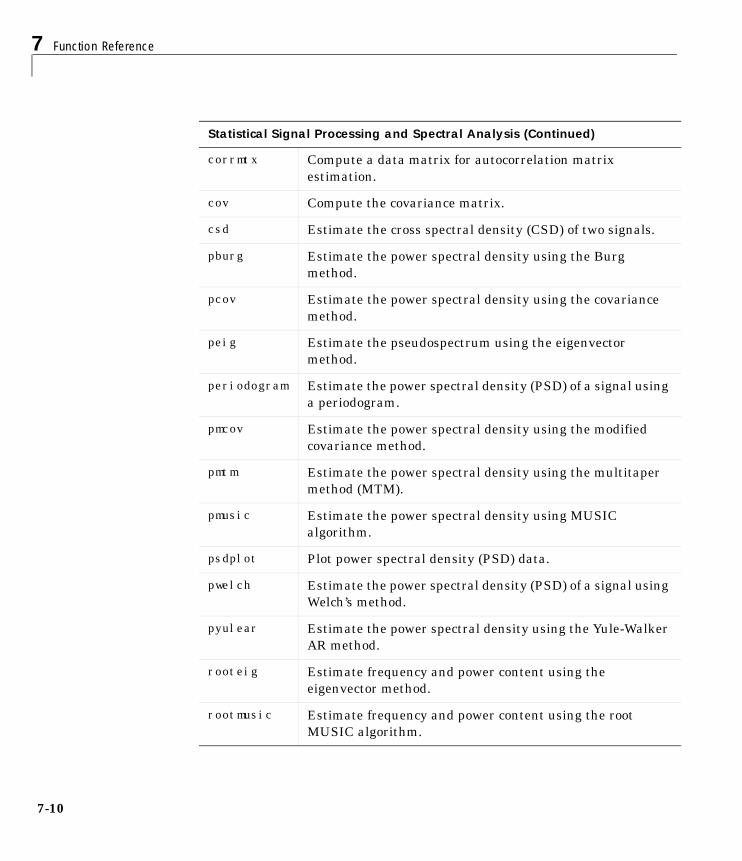
7 Function Reference
7-10
corrmtx Compute a data matrix for autocorrelation matrixestimation.
cov Compute the covariance matrix.
csd Estimate the cross spectral density (CSD) of two signals.
pburg Estimate the power spectral density using the Burgmethod.
pcov Estimate the power spectral density using the covariancemethod.
peig Estimate the pseudospectrum using the eigenvectormethod.
periodogram Estimate the power spectral density (PSD) of a signal usinga periodogram.
pmcov Estimate the power spectral density using the modifiedcovariance method.
pmtm Estimate the power spectral density using the multitapermethod (MTM).
pmusic Estimate the power spectral density using MUSICalgorithm.
psdplot Plot power spectral density (PSD) data.
pwelch Estimate the power spectral density (PSD) of a signal usingWelch’s method.
pyulear Estimate the power spectral density using the Yule-WalkerAR method.
rooteig Estimate frequency and power content using theeigenvector method.
rootmusic Estimate frequency and power content using the rootMUSIC algorithm.
Statistical Signal Processing and Spectral Analysis (Continued)
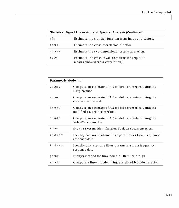
Function Category List
7-11
tfe Estimate the transfer function from input and output.
xcorr Estimate the cross-correlation function.
xcorr2 Estimate the two-dimensional cross-correlation.
xcov Estimate the cross-covariance function (equal tomean-removed cross-correlation).
Parametric Modeling
arburg Compute an estimate of AR model parameters using theBurg method.
arcov Compute an estimate of AR model parameters using thecovariance method.
armcov Compute an estimate of AR model parameters using themodified covariance method.
aryule Compute an estimate of AR model parameters using theYule-Walker method.
ident See the System Identification Toolbox documentation.
invfreqs Identify continuous-time filter parameters from frequencyresponse data.
invfreqz Identify discrete-time filter parameters from frequencyresponse data.
prony Prony’s method for time domain IIR filter design.
stmcb Compute a linear model using Steiglitz-McBride iteration.
Statistical Signal Processing and Spectral Analysis (Continued)
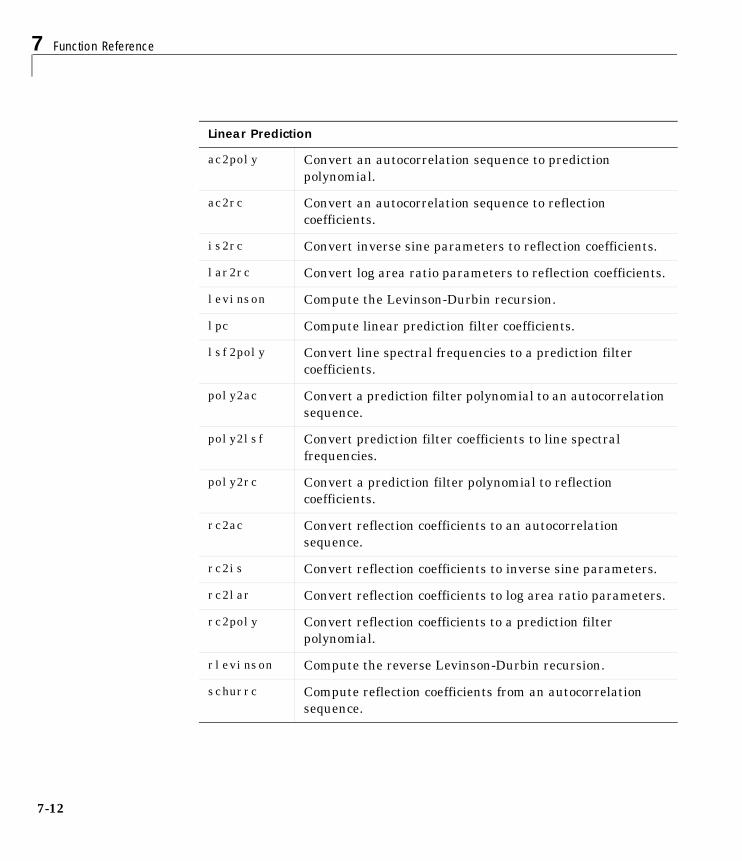
7 Function Reference
7-12
Linear Prediction
ac2poly Convert an autocorrelation sequence to predictionpolynomial.
ac2rc Convert an autocorrelation sequence to reflectioncoefficients.
is2rc Convert inverse sine parameters to reflection coefficients.
lar2rc Convert log area ratio parameters to reflection coefficients.
levinson Compute the Levinson-Durbin recursion.
lpc Compute linear prediction filter coefficients.
lsf2poly Convert line spectral frequencies to a prediction filtercoefficients.
poly2ac Convert a prediction filter polynomial to an autocorrelationsequence.
poly2lsf Convert prediction filter coefficients to line spectralfrequencies.
poly2rc Convert a prediction filter polynomial to reflectioncoefficients.
rc2ac Convert reflection coefficients to an autocorrelationsequence.
rc2is Convert reflection coefficients to inverse sine parameters.
rc2lar Convert reflection coefficients to log area ratio parameters.
rc2poly Convert reflection coefficients to a prediction filterpolynomial.
rlevinson Compute the reverse Levinson-Durbin recursion.
schurrc Compute reflection coefficients from an autocorrelationsequence.
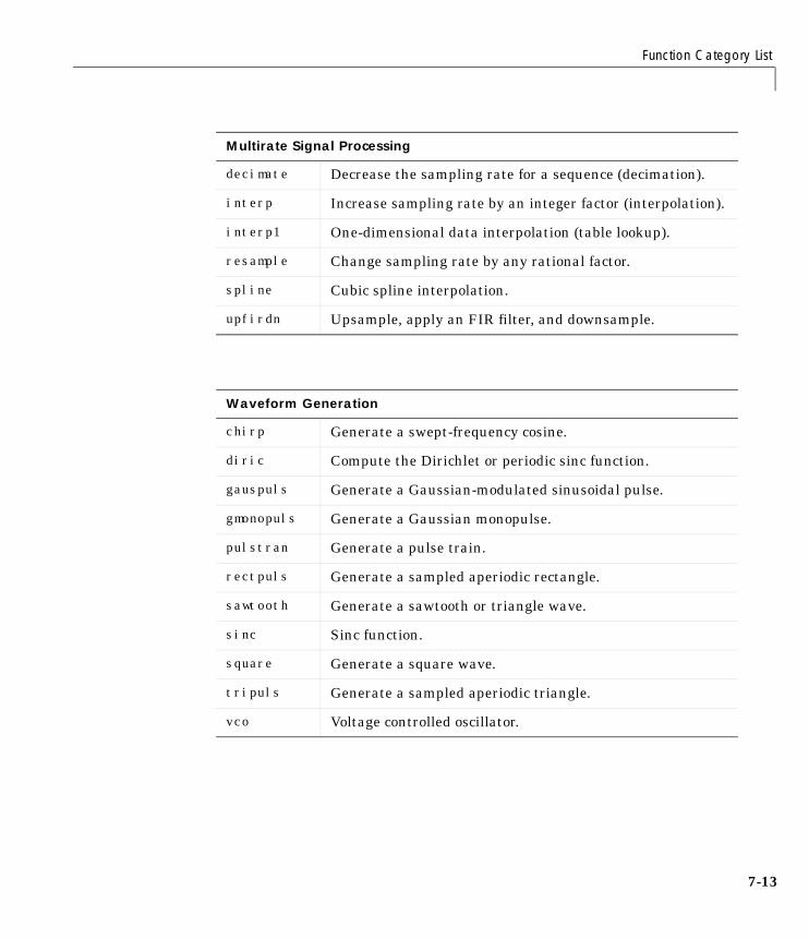
Function Category List
7-13
Multirate Signal Processing
decimate Decrease the sampling rate for a sequence (decimation).
interp Increase sampling rate by an integer factor (interpolation).
interp1 One-dimensional data interpolation (table lookup).
resample Change sampling rate by any rational factor.
spline Cubic spline interpolation.
upfirdn Upsample, apply an FIR filter, and downsample.
Waveform Generation
chirp Generate a swept-frequency cosine.
diric Compute the Dirichlet or periodic sinc function.
gauspuls Generate a Gaussian-modulated sinusoidal pulse.
gmonopuls Generate a Gaussian monopulse.
pulstran Generate a pulse train.
rectpuls Generate a sampled aperiodic rectangle.
sawtooth Generate a sawtooth or triangle wave.
sinc Sinc function.
square Generate a square wave.
tripuls Generate a sampled aperiodic triangle.
vco Voltage controlled oscillator.
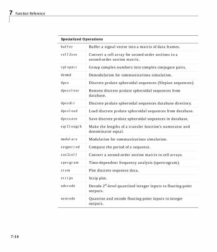
7 Function Reference
7-14
Specialized Operations
buffer Buffer a signal vector into a matrix of data frames.
cell2sos Convert a cell array for second-order sections to asecond-order section matrix.
cplxpair Group complex numbers into complex conjugate pairs.
demod Demodulation for communications simulation.
dpss Discrete prolate spheroidal sequences (Slepian sequences).
dpssclear Remove discrete prolate spheroidal sequences fromdatabase.
dpssdir Discrete prolate spheroidal sequences database directory.
dpssload Load discrete prolate spheroidal sequences from database.
dpsssave Save discrete prolate spheroidal sequences in database.
eqtflength Make the lengths of a transfer function's numerator anddenominator equal.
modulate Modulation for communications simulation.
seqperiod Compute the period of a sequence.
sos2cell Convert a second-order section matrix to cell arrays.
specgram Time-dependent frequency analysis (spectrogram).
stem Plot discrete sequence data.
strips Strip plot.
udecode Decode 2n-level quantized integer inputs to floating-pointoutputs.
uencode Quantize and encode floating-point inputs to integeroutputs.

Function Category List
7-15
Graphical User Interfaces
fdatool Open the Filter Design and Analysis Tool.
sptool Interactive digital signal processing tool (SPTool).
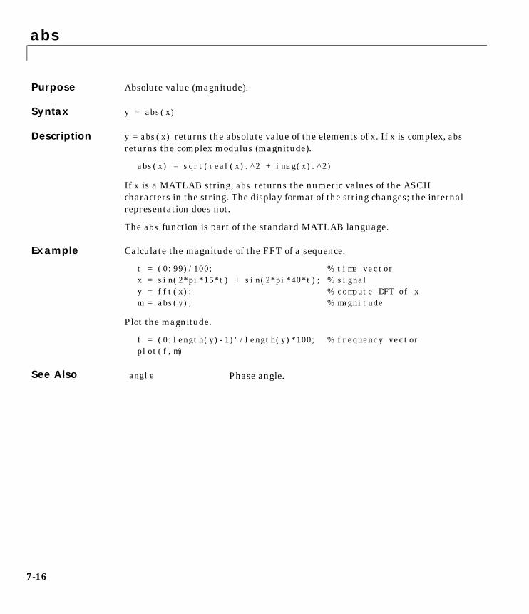
abs
7-16
7absPurpose Absolute value (magnitude).
Syntax y = abs(x)
Description y = abs(x) returns the absolute value of the elements of x. If x is complex, absreturns the complex modulus (magnitude).
abs(x) = sqrt(real(x).^2 + imag(x).^2)
If x is a MATLAB string, abs returns the numeric values of the ASCIIcharacters in the string. The display format of the string changes; the internalrepresentation does not.
The abs function is part of the standard MATLAB language.
Example Calculate the magnitude of the FFT of a sequence.
t = (0:99)/100; % time vectorx = sin(2*pi*15*t) + sin(2*pi*40*t); % signaly = fft(x); % compute DFT of xm = abs(y); % magnitude
Plot the magnitude.
f = (0:length(y)-1)'/length(y)*100; % frequency vectorplot(f,m)
See Also angle Phase angle.

ac2poly
7-17
7ac2polyPurpose Convert an autocorrelation sequence to a prediction filter polynomial.
Syntax a = ac2poly(r)[a,efinal] = ac2poly(r)
Description a = ac2poly(r) finds the prediction filter polynomial a corresponding to theautocorrelation sequence r. a is the same length as r, and a(1) = 1. Theprediction filter polynomial represents the coefficients of the prediction filterwhose output produces a signal whose autocorrelation sequence isapproximately the same as the given autocorrelation sequence r.
[a,efinal] = ac2poly(r) returns the final prediction error efinal,determined by running the filter for length(r) steps.
Remarks You can apply this function to real or complex data.
Example Consider the autocorrelation sequence
r = [5.0000 -1.5450 -3.9547 3.9331 1.4681 -4.7500];
The equivalent prediction filter polynomial is
[a,efinal] = ac2poly(r)
a = 1.0000 0.6147 0.9898 0.0004 0.0034 -0.0077
efinal =
0.1791
See Also
References [1] Kay, S.M. Modern Spectral Estimation. Englewood Cliffs, NJ:Prentice-Hall, 1988.
ac2rc Convert an autocorrelation sequence to reflectioncoefficients.
poly2ac Convert a prediction filter polynomial to anautocorrelation sequence.
rc2poly Convert reflection coefficients to a prediction filterpolynomial.
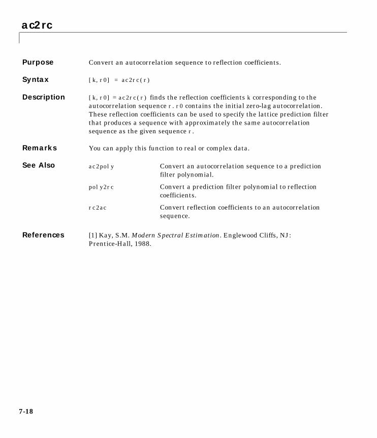
ac2rc
7-18
7ac2rcPurpose Convert an autocorrelation sequence to reflection coefficients.
Syntax [k,r0] = ac2rc(r)
Description [k,r0] = ac2rc(r) finds the reflection coefficients k corresponding to theautocorrelation sequence r. r0 contains the initial zero-lag autocorrelation.These reflection coefficients can be used to specify the lattice prediction filterthat produces a sequence with approximately the same autocorrelationsequence as the given sequence r.
Remarks You can apply this function to real or complex data.
See Also
References [1] Kay, S.M. Modern Spectral Estimation. Englewood Cliffs, NJ:Prentice-Hall, 1988.
ac2poly Convert an autocorrelation sequence to a predictionfilter polynomial.
poly2rc Convert a prediction filter polynomial to reflectioncoefficients.
rc2ac Convert reflection coefficients to an autocorrelationsequence.
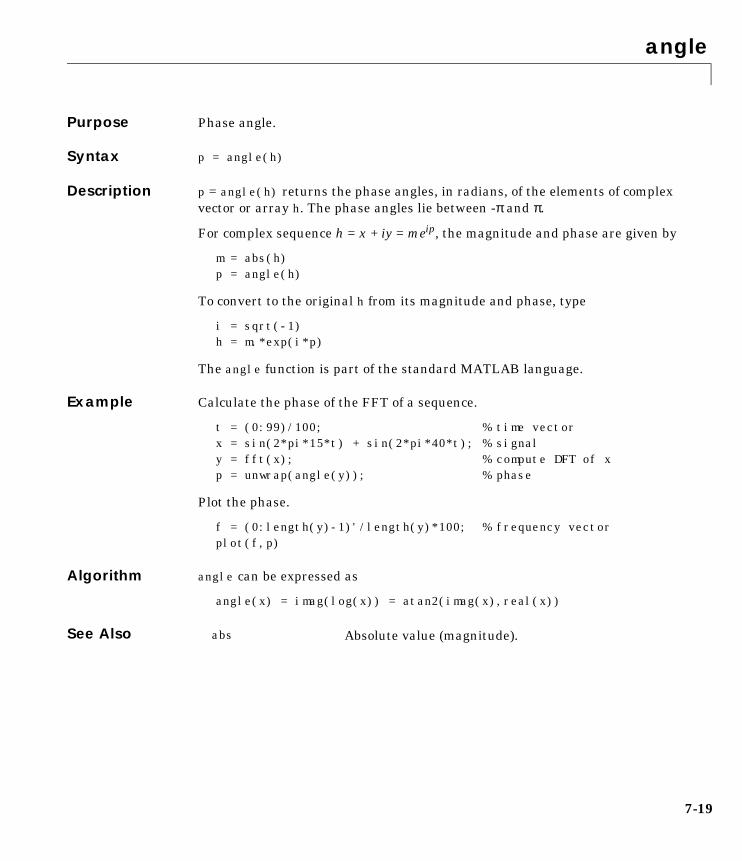
angle
7-19
7anglePurpose Phase angle.
Syntax p = angle(h)
Description p = angle(h) returns the phase angles, in radians, of the elements of complexvector or array h. The phase angles lie between -π and π.
For complex sequence h = x + iy = meip, the magnitude and phase are given by
m = abs(h)p = angle(h)
To convert to the original h from its magnitude and phase, type
i = sqrt(-1)h = m.*exp(i*p)
The angle function is part of the standard MATLAB language.
Example Calculate the phase of the FFT of a sequence.
t = (0:99)/100; % time vectorx = sin(2*pi*15*t) + sin(2*pi*40*t); % signaly = fft(x); % compute DFT of xp = unwrap(angle(y)); % phase
Plot the phase.
f = (0:length(y)-1)'/length(y)*100; % frequency vectorplot(f,p)
Algorithm angle can be expressed as
angle(x) = imag(log(x)) = atan2(imag(x),real(x))
See Also abs Absolute value (magnitude).
arburg
7-20
7arburgPurpose Compute an estimate of AR model parameters using the Burg method.
Syntax a = arburg(x,p)[a,e] = arburg(x,p)[a,e,k] = arburg(x,p)
Description a = arburg(x,p) uses the Burg method to fit a pth order autoregressive (AR)model to the input signal, x, by minimizing (least squares) the forward andbackward prediction errors while constraining the AR parameters to satisfythe Levinson-Durbin recursion. x is assumed to be the output of an AR systemdriven by white noise. Vector a contains the normalized estimate of the ARsystem parameters, A(z), in descending powers of z.
Since the method characterizes the input data using an all-pole model, thecorrect choice of the model order p is important.
[a,e] = arburg(x,p) returns the variance estimate, e, of the white noise inputto the AR model.
[a,e,k] = arburg(x,p) returns a vector, k, of reflection coefficients.
See Also
H z( ) eA z( )------------ e
1 a2z 1– … a p 1+( )zp–
+ + +----------------------------------------------------------------------= =
arcov Compute an estimate of AR model parameters usingthe covariance method.
armcov Compute an estimate of AR model parameters usingthe modified covariance method.
aryule Compute an estimate of AR model parameters usingthe Yule-Walker method.
lpc Compute linear predictive recursion coefficients.
pburg Compute the power spectrum estimate using theBurg method.
prony Prony’s method for time-domain IIR filter design.

arcov
7-21
7arcovPurpose Compute an estimate of AR model parameters using the covariance method.
Syntax a = arcov(x,p)[a,e] = arcov(x,p)
Description a = arcov(x,p) uses the covariance method to fit a pth order autoregressive(AR) model to the input signal, x, which is assumed to be the output of an ARsystem driven by white noise. This method minimizes the forward predictionerror in the least-squares sense. Vector a contains the normalized estimate ofthe AR system parameters, A(z), in descending powers of z.
Because the method characterizes the input data using an all-pole model, thecorrect choice of the model order p is important.
[a,e] = arcov(x,p) returns the variance estimate, e, of the white noise inputto the AR model.
See Also
H z( ) eA z( )------------ e
1 a2z 1– … a p 1+( )zp–
+ + +----------------------------------------------------------------------= =
arburg Compute an estimate of AR model parameters usingthe Burg method.
armcov Compute an estimate of AR model parameters usingthe modified covariance method.
aryule Compute an estimate of AR model parameters usingthe Yule-Walker method.
lpc Compute linear predictive recursion coefficients.
pcov Estimate the power spectrum using the covariancemethod.
prony Prony’s method for IIR filter design.
armcov
7-22
7armcovPurpose Compute an estimate of AR model parameters using the modified covariancemethod.
Syntax a = armcov(x,p)[a,e] = armcov(x,p)
Description a = armcov(x,p) uses the modified covariance method to fit a pth orderautoregressive (AR) model to the input signal, x, which is assumed to be theoutput of an AR system driven by white noise. This method minimizes theforward and backward prediction errors in the least-squares sense. Vector acontains the normalized estimate of the AR system parameters, A(z), indescending powers of z.
Because the method characterizes the input data using an all-pole model, thecorrect choice of the model order p is important.
[a,e] = armcov(x,p) returns the variance estimate, e, of the white noise inputto the AR model.
See Also
H z( ) eA z( )------------ e
1 a2z 1– … a p 1+( )zp–
+ + +----------------------------------------------------------------------= =
arburg Compute an estimate of AR model parameters usingthe Burg method.
arcov Compute an estimate of AR model parameters usingthe covariance method.
aryule Compute an estimate of AR model parameters usingthe Yule-Walker method.
lpc Compute linear predictive recursion coefficients.
pmcov Estimate the power spectrum using the modifiedcovariance method.
prony Prony’s method for IIR filter design.
aryule
7-23
7aryulePurpose Compute an estimate of AR model parameters using the Yule-Walker method.
Syntax a = aryule(x,p)[a,e] = aryule(x,p)[a,e,k] = aryule(x,p)
Description a = aryule(x,p) uses the Yule-Walker method, also called the autocorrelationmethod, to fit a pth order autoregressive (AR) model to the windowed inputsignal, x, by minimizing the forward prediction error in the least-squaressense. This formulation leads to the Yule-Walker equations, which are solvedby the Levinson-Durbin recursion. x is assumed to be the output of an ARsystem driven by white noise. Vector a contains the normalized estimate of theAR system parameters, A(z), in descending powers of z.
Because the method characterizes the input data using an all-pole model, thecorrect choice of the model order p is important.
[a,e] = aryule(x,p) returns the variance estimate, e, of the white noise inputto the AR model.
[a,e,k] = aryule(x,p) returns a vector, k, of reflection coefficients.
See Also
H z( ) eA z( )------------ e
1 a2z 1– … a p 1+( )zp–
+ + +----------------------------------------------------------------------= =
arburg Compute an estimate of AR model parameters usingthe Burg method.
arcov Compute an estimate of AR model parameters usingthe covariance method.
armcov Compute an estimate of AR model parameters usingthe modified covariance method.
lpc Compute linear predictive recursion coefficients.
prony Prony’s method for IIR filter design.
pyulear Estimate the power spectrum using the Yule-Walkerautoregressive approach.
bartlett
7-24
7bartlettPurpose Compute a Bartlett window.
Syntax w = bartlett(n)
Description w = bartlett(n) returns an n-point Bartlett window in the column vector w,where n must be a positive integer. The coefficients of a Bartlett window arecomputed as follows:
• For n odd
• For n even
The Bartlett window is very similar to a triangular window as returned by thetriang function. The Bartlett window always ends with zeros at samples 1 andn, however, while the triangular window is nonzero at those points. For n odd,the center n-2 points of bartlett(n) are equivalent to triang(n-2).
Note If you specify a one-point window (set n=1), the value 1 is returned.
Example w = bartlett(64);plot(w)title('Bartlett Window')
w k 1+[ ]
2kn 1–------------- 0 k n 1–
2-------------≤ ≤,
2 2 k( )n 1–-------------–
n 1–2
------------- k n 1–≤ ≤,
=
w k 1+[ ]
2 k( )n 1–------------- 0 k n
2--- 1–≤ ≤,
2 n k– 1–( )n 1–
------------------------------ n2--- k n 1–≤ ≤,
=
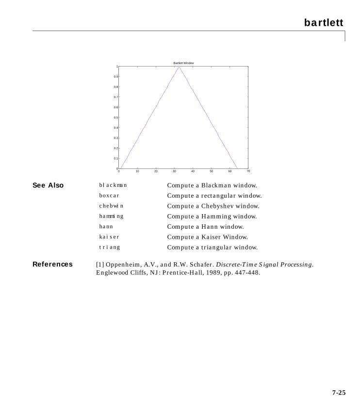
bartlett
7-25
See Also
References [1] Oppenheim, A.V., and R.W. Schafer. Discrete-Time Signal Processing.Englewood Cliffs, NJ: Prentice-Hall, 1989, pp. 447-448.
0 10 20 30 40 50 60 700
0.1
0.2
0.3
0.4
0.5
0.6
0.7
0.8
0.9
1Bartlett Window
blackman Compute a Blackman window.
boxcar Compute a rectangular window.
chebwin Compute a Chebyshev window.
hamming Compute a Hamming window.
hann Compute a Hann window.
kaiser Compute a Kaiser Window.
triang Compute a triangular window.
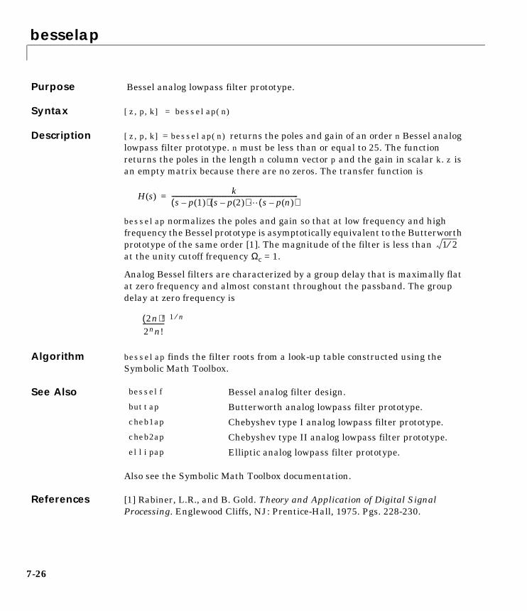
besselap
7-26
7besselapPurpose Bessel analog lowpass filter prototype.
Syntax [z,p,k] = besselap(n)
Description [z,p,k] = besselap(n) returns the poles and gain of an order n Bessel analoglowpass filter prototype. n must be less than or equal to 25. The functionreturns the poles in the length n column vector p and the gain in scalar k. z isan empty matrix because there are no zeros. The transfer function is
besselap normalizes the poles and gain so that at low frequency and highfrequency the Bessel prototype is asymptotically equivalent to the Butterworthprototype of the same order [1]. The magnitude of the filter is less than at the unity cutoff frequency Ωc = 1.
Analog Bessel filters are characterized by a group delay that is maximally flatat zero frequency and almost constant throughout the passband. The groupdelay at zero frequency is
Algorithm besselap finds the filter roots from a look-up table constructed using theSymbolic Math Toolbox.
See Also
Also see the Symbolic Math Toolbox documentation.
References [1] Rabiner, L.R., and B. Gold. Theory and Application of Digital SignalProcessing. Englewood Cliffs, NJ: Prentice-Hall, 1975. Pgs. 228-230.
H s( )k
s p 1( )–( ) s p 2( )–( ) s p n( )–( )--------------------------------------------------------------------------------=
1 2⁄
2n( )!2nn!-------------- 1 n⁄
besself Bessel analog filter design.
buttap Butterworth analog lowpass filter prototype.
cheb1ap Chebyshev type I analog lowpass filter prototype.
cheb2ap Chebyshev type II analog lowpass filter prototype.
ellipap Elliptic analog lowpass filter prototype.
besself
7-27
7besselfPurpose Bessel analog filter design.
Syntax [b,a] = besself(n,Wn)[b,a] = besself(n,Wn,'ftype')[z,p,k] = besself(...)[A,B,C,D] = besself(...)
Description besself designs lowpass, bandpass, highpass, and bandstop analog Besselfilters. Analog Bessel filters are characterized by almost constant group delayacross the entire passband, thus preserving the wave shape of filtered signalsin the passband. Digital Bessel filters do not retain this quality, and besselftherefore does not support the design of digital Bessel filters.
[b,a] = besself(n,Wn) designs an order n lowpass analog filter with cutofffrequency Wn. It returns the filter coefficients in the length n+1 row vectors band a, with coefficients in descending powers of s, derived from the transferfunction
Cutoff frequency is the frequency at which the magnitude response of the filterbegins to decrease significantly. For besself, the cutoff frequency Wn must begreater than 0. The magnitude response of a Bessel filter designed by besselfis always less than at the cutoff frequency, and it decreases as the ordern increases.
If Wn is a two-element vector, Wn = [w1 w2] with w1 < w2, then besself(n,Wn) returns an order 2*n bandpass analog filter with passband w1 < ω < w2.
[b,a] = besself(n,Wn,'ftype') designs a highpass or bandstop filter, wherethe string 'ftype' is:
• 'high' for a highpass analog filter with cutoff frequency Wn
• 'stop' for an order 2*n bandstop analog filter if Wn is a two-element vector,Wn = [w1 w2]
The stopband is w1 < ω < w2.
H s( )B s( )A s( )----------- b 1( )sn b 2( )sn 1– b n 1+( )+ + +
sn a 2( )sn 1– a n 1+( )+ + +-------------------------------------------------------------------------------------= =
1 2⁄
besself
7-28
With different numbers of output arguments, besself directly obtains otherrealizations of the analog filter. To obtain zero-pole-gain form, use three outputarguments as shown below.
[z,p,k] = besself(n,Wn) or
[z,p,k] = besself(n,Wn,'ftype') returns the zeros and poles in length n or2*n column vectors z and p and the gain in the scalar k.
To obtain state-space form, use four output arguments as shown below.
[A,B,C,D] = besself(n,Wn) or
[A,B,C,D] = besself(n,Wn,'ftype') where A, B, C, and D are
and u is the input, x is the state vector, and y is the output.
Example Design a fifth-order analog lowpass Bessel filter that suppresses frequenciesgreater than 10,000 rad/s and plot the frequency response of the filter usingfreqs.
[b,a] = besself(5,10000);freqs(b,a) % Plot frequency response
x· Ax Bu+=
y Cx Du+=
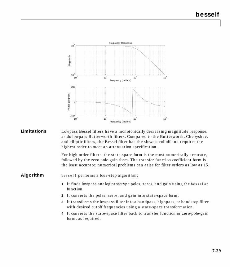
besself
7-29
Limitations Lowpass Bessel filters have a monotonically decreasing magnitude response,as do lowpass Butterworth filters. Compared to the Butterworth, Chebyshev,and elliptic filters, the Bessel filter has the slowest rolloff and requires thehighest order to meet an attenuation specification.
For high order filters, the state-space form is the most numerically accurate,followed by the zero-pole-gain form. The transfer function coefficient form isthe least accurate; numerical problems can arise for filter orders as low as 15.
Algorithm besself performs a four-step algorithm:
1 It finds lowpass analog prototype poles, zeros, and gain using the besselapfunction.
2 It converts the poles, zeros, and gain into state-space form.
3 It transforms the lowpass filter into a bandpass, highpass, or bandstop filterwith desired cutoff frequencies using a state-space transformation.
4 It converts the state-space filter back to transfer function or zero-pole-gainform, as required.
102
103
104
105
-200
0
200
Frequency (radians)
Pha
se (
degr
ees)
102
103
104
105
10-5
100
Frequency (radians)
Mag
nitu
de
Frequency Response

besself
7-30
See Also besselap Bessel analog lowpass filter prototype.
butter Butterworth analog and digital filter design.
cheby1 Chebyshev type I filter design (passband ripple).
cheby2 Chebyshev type II filter design (stopband ripple).
ellip Elliptic (Cauer) filter design.
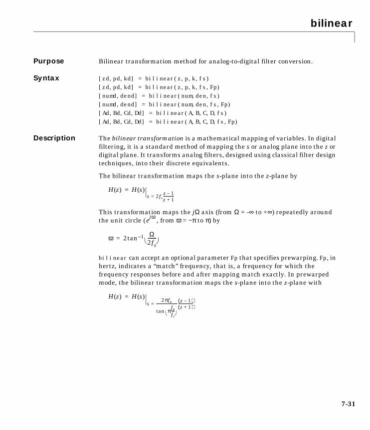
bilinear
7-31
7bilinearPurpose Bilinear transformation method for analog-to-digital filter conversion.
Syntax [zd,pd,kd] = bilinear(z,p,k,fs)[zd,pd,kd] = bilinear(z,p,k,fs,Fp)[numd,dend] = bilinear(num,den,fs)[numd,dend] = bilinear(num,den,fs,Fp)[Ad,Bd,Cd,Dd] = bilinear(A,B,C,D,fs)[Ad,Bd,Cd,Dd] = bilinear(A,B,C,D,fs,Fp)
Description The bilinear transformation is a mathematical mapping of variables. In digitalfiltering, it is a standard method of mapping the s or analog plane into the z ordigital plane. It transforms analog filters, designed using classical filter designtechniques, into their discrete equivalents.
The bilinear transformation maps the s-plane into the z-plane by
This transformation maps the jΩ axis (from Ω = -∞ to +∞) repeatedly aroundthe unit circle ( , from ω = −π to π) by
bilinear can accept an optional parameter Fp that specifies prewarping. Fp, inhertz, indicates a “match” frequency, that is, a frequency for which thefrequency responses before and after mapping match exactly. In prewarpedmode, the bilinear transformation maps the s-plane into the z-plane with
H z( ) H s( )s 2fs
z 1–z 1+------------=
=
ejω
ω 2tan 1– Ω2fs-------- =
H z( ) H s( )s
2πfp
πfp
fs
---- tan
------------------------ z 1–( )z 1+( )
-----------------==

bilinear
7-32
With the prewarping option, bilinear maps the jΩ axis (from Ω = -∞ to +∞)repeatedly around the unit circle ( , from ω = −π to π) by
In prewarped mode, bilinear matches the frequency 2πfp (in radians persecond) in the s-plane to the normalized frequency 2πfp/fs (in radians persecond) in the z-plane.
The bilinear function works with three different linear systemrepresentations: zero-pole-gain, transfer function, and state-space form.
Zero-Pole-Gain
[zd,pd,kd] = bilinear(z,p,k,fs) and
[zd,pd,kd] = bilinear(z,p,k,fs,Fp) convert the s-domain transfer functionspecified by z, p, and k to a discrete equivalent. Inputs z and p are columnvectors containing the zeros and poles, k is a scalar gain, and fs is the samplingfrequency in hertz. bilinear returns the discrete equivalent in column vectorszd and pd and scalar kd. Fp is the optional match frequency, in hertz, forprewarping.
Transfer Function
[numd,dend] = bilinear(num,den,fs) and
[numd,dend] = bilinear(num,den,fs,Fp) convert an s-domain transferfunction given by num and den to a discrete equivalent. Row vectors num and denspecify the coefficients of the numerator and denominator, respectively, indescending powers of s.
ejω
ω 2tan 1–Ω π
fpfs----
tan
2πfp-----------------------------
=
num s( )den s( )-------------------- num 1( )snn num nn( )s num nn 1+( )+ + +
den 1( )snd den nd( )s den nd 1+( )+ + +----------------------------------------------------------------------------------------------------------------------=

bilinear
7-33
fs is the sampling frequency in hertz. bilinear returns the discrete equivalentin row vectors numd and dend in descending powers of z (ascending powersof z-1). Fp is the optional match frequency, in hertz, for prewarping.
State-Space
[Ad,Bd,Cd,Dd] = bilinear(A,B,C,D,fs) and
[Ad,Bd,Cd,Dd] = bilinear(A,B,C,D,fs,Fp) convert the continuous-timestate-space system in matrices A, B, C, D,
to the discrete-time system
fs is the sampling frequency in hertz. bilinear returns the discrete equivalentin matrices Ad, Bd, Cd, Dd. Fp is the optional match frequency, in hertz, forprewarping.
Algorithm bilinear uses one of two algorithms depending on the format of the inputlinear system you supply. One algorithm works on the zero-pole-gain formatand the other on the state-space format. For transfer function representations,bilinear converts to state-space form, performs the transformation, andconverts the resulting state-space system back to transfer function form.
Zero-Pole-Gain AlgorithmFor a system in zero-pole-gain form, bilinear performs four steps:
1 If Fp is present, k = 2*pi*Fp/tan(pi*Fp/fs); otherwise k = 2*fs.
2 It strips any zeros at ±∞ using z = z(find(finite(z)));
x· Ax Bu+=
y Cx Du+=
x n 1+[ ] Adx n[ ] Bdu n[ ]+=
y n[ ] Cdx n[ ] Ddu n[ ]+=

bilinear
7-34
3 It transforms the zeros, poles, and gain using pd = (1+p/k)./(1-p/k); zd = (1+z/k)./(1-z/k); kd = real(k*prod(fs-z)./prod(fs-p));
4 It adds extra zeros at -1 so the resulting system has equivalent numeratorand denominator order.
State-Space AlgorithmFor a system in state-space form, bilinear performs two steps:
1 If Fp is present, k = 2*pi*Fp/tan(pi*Fp/fs); else k = 2*fs.
2 It computes Ad, Bd, Cd, and Dd in terms of A, B, C, and D using
bilinear implements these relations using conventional MATLABstatements. The scalar r is arbitrary; bilinear uses to ensure goodquantization noise properties in the resulting system.
Diagnostics bilinear requires that the numerator order be no greater than thedenominator order. If this is not the case, bilinear displays
Numerator cannot be higher order than denominator.
For bilinear to distinguish between the zero-pole-gain and transfer functionlinear system formats, the first two input parameters must be vectors with thesame orientation in these cases. If this is not the case, bilinear displays
First two arguments must have the same orientation.
Ad I 1k--- A+
I 1
k--- A–
1–=
Bd2kr
------- I 1k--- A–
1–B=
Cd rC I 1k--- A–
1–
=
Dd1k--- C I 1
k--- A–
1–B D+=
r 2 k⁄=

bilinear
7-35
See Also
References [1] Parks, T.W., and C.S. Burrus. Digital Filter Design. New York: John Wiley& Sons, 1987. Pgs. 209-213.
[2] Oppenheim, A.V., and R.W. Schafer. Discrete-Time Signal Processing.Englewood Cliffs, NJ: Prentice-Hall, 1989. Pgs. 415-430.
impinvar Analog to digital conversion using the impulseinvariance method.
lp2bp Transform lowpass analog filters to bandpass.
lp2bs Transform lowpass analog filters to bandstop.
lp2hp Transform lowpass analog filters to highpass.
lp2lp Change the cut-off frequency for lowpass analogfilters.

blackman
7-36
7blackmanPurpose Compute a Blackman window.
Syntax w = blackman(n)w = blackman(n,'sflag')
Description w = blackman(n) returns the n-point symmetric Blackman window in thecolumn vector w, where n is a positive integer.
w = blackman(n,'sflag') returns an n-point Blackman window using thewindow sampling specified by 'sflag', which can be either 'periodic' or'symmetric' (the default). When 'periodic' is specified, blackman computesa length n+1 window and returns the first n points.
Note If you specify a one-point window (set n=1), the value 1 is returned.
Algorithm The equation for computing the coefficients of a Blackman window is
Blackman windows have slightly wider central lobes and less sideband leakagethan equivalent length Hamming and Hann windows.
Examples w = blackman(64);plot(w)title('Blackman Window')
w k 1+[ ] 0.42 0.5 2π kn 1–-------------
cos– 0.08 4π k
n 1–-------------
cos+ k 0= … n 1–, , ,=
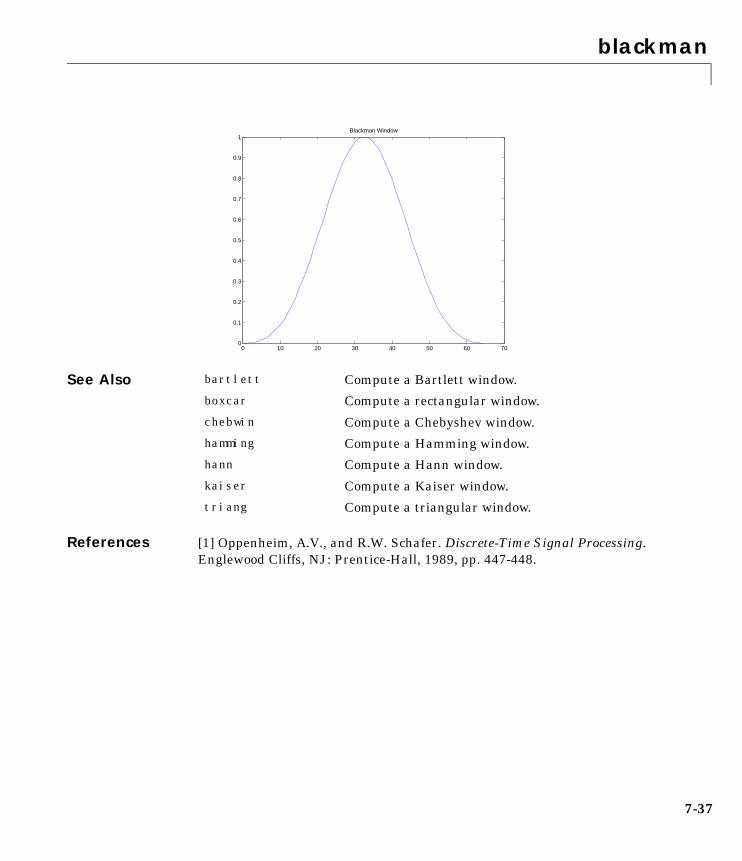
blackman
7-37
See Also
References [1] Oppenheim, A.V., and R.W. Schafer. Discrete-Time Signal Processing.Englewood Cliffs, NJ: Prentice-Hall, 1989, pp. 447-448.
0 10 20 30 40 50 60 700
0.1
0.2
0.3
0.4
0.5
0.6
0.7
0.8
0.9
1Blackman Window
bartlett Compute a Bartlett window.
boxcar Compute a rectangular window.
chebwin Compute a Chebyshev window.
hamming Compute a Hamming window.
hann Compute a Hann window.
kaiser Compute a Kaiser window.
triang Compute a triangular window.
boxcar
7-38
7boxcarPurpose Compute a rectangular window.
Syntax w = boxcar(n)
Description w = boxcar(n) returns a rectangular window of length n in the column vector w.This function is provided for completeness; a rectangular window is equivalentto no window at all.
Algorithm w = ones(n,1);
See Also
References [1] Oppenheim, A.V., and R.W. Schafer. Discrete-Time Signal Processing.Englewood Cliffs, NJ: Prentice-Hall, 1989, pp. 447-448.
bartlett Compute a Bartlett window.
blackman Compute a Blackman window.
chebwin Compute a Chebyshev window.
hamming Compute a Hamming window.
hann Compute a Hann window.
kaiser Compute a Kaiser window.
triang Compute a triangular window.

buffer
7-39
7bufferPurpose Buffer a signal vector into a matrix of data frames.
Syntax y = buffer(x,n)y = buffer(x,n,p)y = buffer(x,n,p,opt)[y,z] = buffer(...)[y,z,opt] = buffer(...)
Description y = buffer(x,n) partitions a length-L signal vector x into nonoverlapping datasegments (frames) of length n. Each data frame occupies one column of matrixoutput y, which has n rows and ceil(L/n) columns. If L is not evenly divisibleby n, the last column is zero-padded to length n.
y = buffer(x,n,p) overlaps or underlaps successive frames in the outputmatrix by p samples:
• For 0 < p < n (overlap), buffer repeats the final p samples of each frame atthe beginning of the following frame. For example, if x = 1:30 and n = 7, anoverlap of p = 3 looks like this.
The first frame starts with p zeros (the default initial condition), and thenumber of columns in y is ceil(L/(n-p)).
y = 0 2 6 10 14 18 22 26 0 3 7 11 15 19 23 27 0 4 8 12 16 20 24 28 1 5 9 13 17 21 25 29 2 6 10 14 18 22 26 30 3 7 11 15 19 23 27 0 4 8 12 16 20 24 28 0
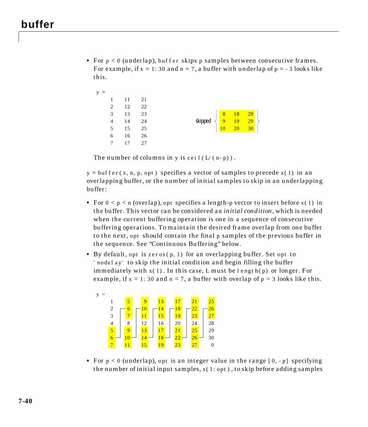
buffer
7-40
• For p < 0 (underlap), buffer skips p samples between consecutive frames.For example, if x = 1:30 and n = 7, a buffer with underlap of p = -3 looks likethis.
The number of columns in y is ceil(L/(n-p)).
y = buffer(x,n,p,opt) specifies a vector of samples to precede x(1) in anoverlapping buffer, or the number of initial samples to skip in an underlappingbuffer:
• For 0 < p < n (overlap), opt specifies a length-p vector to insert before x(1) inthe buffer. This vector can be considered an initial condition, which is neededwhen the current buffering operation is one in a sequence of consecutivebuffering operations. To maintain the desired frame overlap from one bufferto the next, opt should contain the final p samples of the previous buffer inthe sequence. See “Continuous Buffering” below.
• By default, opt is zeros(p,1) for an overlapping buffer. Set opt to'nodelay' to skip the initial condition and begin filling the bufferimmediately with x(1). In this case, L must be length(p) or longer. Forexample, if x = 1:30 and n = 7, a buffer with overlap of p = 3 looks like this.
• For p < 0 (underlap), opt is an integer value in the range [0,-p] specifyingthe number of initial input samples, x(1:opt), to skip before adding samples
y = 1 11 21 2 12 22 3 13 23 4 14 24 5 15 25 6 16 26 7 17 27
8 18 289 19 2910 20 30
skipped
y = 1 5 9 13 17 21 25 2 6 10 14 18 22 26 3 7 11 15 19 23 27 4 8 12 16 20 24 28 5 9 13 17 21 25 29 6 10 14 18 22 26 30 7 11 15 19 23 27 0
buffer
7-41
to the buffer. The first value in the buffer is therefore x(opt+1). By default,opt is zero for an underlapping buffer.
This option is especially useful when the current buffering operation is onein a sequence of consecutive buffering operations. To maintain the desiredframe underlap from one buffer to the next, opt should equal the differencebetween the total number of points to skip between frames (p) and thenumber of points that were available to be skipped in the previous input tobuffer. If the previous input had fewer than p points that could be skippedafter filling the final frame of that buffer, the remaining opt points need tobe removed from the first frame of the current buffer. See “ContinuousBuffering” below for an example of how this works in practice.
[y,z] = buffer(...) partitions the length-L signal vector x into frames oflength n, and outputs only the full frames in y. If y is an overlapping buffer, ithas n rows and m columns, where
m = floor(L/(n-p)) % When length(opt) = p
or
m = floor((L-n)/(n-p))+1 % When opt = 'nodelay'
If y is an underlapping buffer, it has n rows and m columns, where
m = floor((L-opt)/(n-p)) + (rem((L-opt),(n-p)) >= n)
If the number of samples in the input vector (after the appropriate overlappingor underlapping operations) exceeds the number of places available in then-by-m buffer, the remaining samples in x are output in vector z, which for anoverlapping buffer has length
length(z) = L - m*(n-p) % When length(opt) = p
or
length(z) = L - ((m-1)*(n-p)+n)% When opt = 'nodelay'
and for an underlapping buffer has length
length(z) = (L-opt) - m*(n-p)
buffer
7-42
Output z shares the same orientation (row or column) as x. If there are noremaining samples in the input after the buffer with the specified overlap orunderlap is filled, z is an empty vector.
[y,z,opt] = buffer(...) returns the last p samples of a overlapping buffer inoutput opt. In an underlapping buffer, opt is the difference between the totalnumber of points to skip between frames (-p) and the number of points in x thatwere available to be skipped after filling the last frame:
• For 0 < p < n (overlap), opt (as an output) contains the final p samples in thelast frame of the buffer. This vector can be used as the initial condition for asubsequent buffering operation in a sequence of consecutive bufferingoperations. This allows the desired frame overlap to be maintained from onebuffer to the next. See “Continuous Buffering” below.
• For p < 0 (underlap), opt (as an output) is the difference between the totalnumber of points to skip between frames (-p) and the number of points in xthat were available to be skipped after filling the last frame.opt = m*(n-p) + opt - L % z is the empty vector.
where opt on the right-hand side is the input argument to buffer, and opton the left-hand side is the output argument. Here m is the number ofcolumns in the buffer, which ism = floor((L-opt)/(n-p)) + (rem((L-opt),(n-p))>=n)
Note that for an underlapping buffer output opt is always zero whenoutput z contains data.
The opt output for an underlapping buffer is especially useful when thecurrent buffering operation is one in a sequence of consecutive bufferingoperations. The opt output from each buffering operation specifies thenumber of samples that need to be skipped at the start of the next bufferingoperation to maintain the desired frame underlap from one buffer to thenext. If fewer than p points were available to be skipped after filling the finalframe of the current buffer, the remaining opt points need to be removedfrom the first frame of the next buffer.
In a sequence of buffering operations, the opt output from each operationshould be used as the opt input to the subsequent buffering operation. Thisensures that the desired frame overlap or underlap is maintained from buffer

buffer
7-43
to buffer, as well as from frame to frame within the same buffer. See“Continuous Buffering” below for an example of how this works in practice.
Continuous BufferingIn a continuous buffering operation, the vector input to the buffer functionrepresents one frame in a sequence of frames that make up a discrete signal.These signal frames can originate in a frame-based data acquisition process, orwithin a frame-based algorithm like the FFT.
As an example, you might acquire data from an A/D card in frames of 64samples. In the simplest case, you could rebuffer the data into frames of 16samples; buffer with n = 16 creates a buffer of four frames from each64-element input frame. The result is that the signal of frame size 64 has beenconverted to a signal of frame size 16; no samples were added or removed.
In the general case where the original signal frame size, L, is not equallydivisible by the new frame size, n, the overflow from the last frame needs to becaptured and recycled into the following buffer. You can do this by iterativelycalling buffer on input x with the two-output-argument syntax.
[y,z] = buffer([z;x],n) % x is a column vector.
[y,z] = buffer([z,x],n) % x is a row vector.
This simply captures any buffer overflow in z, and prepends the data to thesubsequent input in the next call to buffer. Again, the input signal, x, of framesize L, has been converted to a signal of frame size n without any insertion ordeletion of samples.
Note that continuous buffering cannot be done with the single-output syntaxy = buffer(...), because the last frame of y in this case is zero padded, whichadds new samples to the signal.
Continuous buffering in the presence of overlap and underlap is handled withthe opt parameter, which is used as both an input and output to buffer. Thefollowing two examples demonstrate how the opt parameter should be used.
buffer
7-44
Examples Example 1: Continuous Overlapping BuffersFirst create a buffer containing 100 frames, each with 11 samples.
data = buffer(1:1100,11); % 11 samples per frame
Imagine that the frames (columns) in the matrix called data are the sequentialoutputs of a data acquisition board sampling a physical signal: data(:,1) isthe first D/A output, containing the first 11 signal samples; data(:,2) is thesecond output, containing the next 11 signal samples, and so on.
You want to rebuffer this signal from the acquired frame size of 11 to a framesize of 4 with an overlap of 1. To do this, you will repeatedly call buffer tooperate on each successive input frame, using the opt parameter to maintainconsistency in the overlap from one buffer to the next.
Set the buffer parameters.
n = 4; % New frame sizep = 1; % Overlapopt = -5; % Value of y(1)z = []; % Initialize the carry-over vector.
Now repeatedly call buffer, each time passing in a new signal frame fromdata. Note that overflow samples (returned in z) are carried over andprepended to the input in the subsequent call to buffer.
for i=1:size(data,2), % Loop over each source frame (column). x = data(:,i); % A single frame of the D/A output
[y,z,opt] = buffer([z;x],n,p,opt);
disp(y); % Display the buffer of data.pause
end

buffer
7-45
Here’s what happens during the first four iterations.
Note that the size of the output matrix, y, can vary by a single column from oneiteration to the next. This is typical for buffering operations with overlap orunderlap.
[1:11]i=1
5– 3 61 4 72 5 83 6 9
Iteration Input frame [z;x]' opt (input) opt (output) Output buffer (y) Overflow (z)
[10 11]–5 9
i=2 [10 11 12:22] 9 21
9 12 15 1810 13 16 1911 14 17 2012 15 18 21
[22]
i=3 [22 23:33] 21 33
21 24 27 3022 25 28 3123 26 29 3224 27 30 33
[]
33 36 3934 37 4035 38 4136 39 42
[43 44]42[34:44]i=4 33
buffer
7-46
Example 2: Continuous Underlapping BuffersAgain create a buffer containing 100 frames, each with 11 samples.
data = buffer(1:1100,11); % 11 samples per frame
Again, imagine that data(:,1) is the first D/A output, containing the first 11signal samples; data(:,2) is the second output, containing the next 11 signalsamples, and so on.
You want to rebuffer this signal from the acquired frame size of 11 to a framesize of 4 with an underlap of 2. To do this, you will repeatedly call buffer tooperate on each successive input frame, using the opt parameter to maintainconsistency in the underlap from one buffer to the next.
Set the buffer parameters.
n = 4; % New frame sizep = -2; % Underlapopt = 1; % Skip the first input element, x(1).z = []; % Initialize the carry-over vector.
Now repeatedly call buffer, each time passing in a new signal frame fromdata. Note that overflow samples (returned in z) are carried over andprepended to the input in the subsequent call to buffer.
for i=1:size(data,2), % Loop over each source frame (column). x = data(:,i); % A single frame of the D/A output
[y,z,opt] = buffer([z;x],n,p,opt);
disp(y); % Display the buffer of data.pause
end
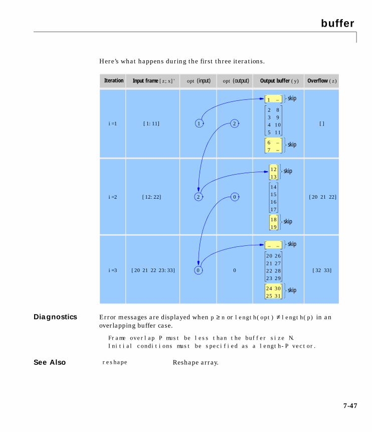
buffer
7-47
Here’s what happens during the first three iterations.
Diagnostics Error messages are displayed when p ≥ n or length(opt) ≠ length(p) in anoverlapping buffer case.
Frame overlap P must be less than the buffer size N.Initial conditions must be specified as a length-P vector.
See Also
[1:11]i=1
2 83 94 105 11
Iteration Input frame [z;x]' opt (input) opt (output) Output buffer (y) Overflow (z)
[]1 2
i=2 [12:22] 2 0
14151617
[20 21 22]
i=3 [20 21 22 23:33] 0 0
20 2621 2722 2823 29
[32 33]
6 –7 –
1 –
1819
1213
– –
24 3025 31
skip
skip
skip
skip
skip
skip
reshape Reshape array.

buttap
7-48
7buttapPurpose Butterworth analog lowpass filter prototype.
Syntax [z,p,k] = buttap(n)
Description [z,p,k] = buttap(n) returns the poles and gain of an order n Butterworthanalog lowpass filter prototype. The function returns the poles in the length ncolumn vector p and the gain in scalar k. z is an empty matrix because thereare no zeros. The transfer function is
Butterworth filters are characterized by a magnitude response that ismaximally flat in the passband and monotonic overall. In the lowpass case, thefirst 2n–1 derivatives of the squared magnitude response are zero at ω = 0. Thesquared magnitude response function is
corresponding to a transfer function with poles equally spaced around a circlein the left half plane. The magnitude response at the cutoff frequency ω0 isalways regardless of the filter order. buttap sets ω0 to 1 for a normalizedresult.
Algorithm z = [];p = exp(sqrt(-1)*(pi*(1:2:2*n-1)/(2*n)+pi/2)).';k = real(prod(-p));
See Also
References [1] Parks, T.W., and C.S. Burrus. Digital Filter Design. New York: John Wiley& Sons, 1987. Chapter 7.
H s( )z s( )p s( )---------- k
s p 1( )–( ) s p 2( )–( ) s p n( )–( )--------------------------------------------------------------------------------= =
H ω( ) 2 11 ω ω0⁄( )2n+------------------------------------=
1 2⁄
besselap Bessel analog lowpass filter prototype.
butter Butterworth analog and digital filter design.
cheb1ap Chebyshev type I analog lowpass filter prototype.
cheb2ap Chebyshev type II analog lowpass filter prototype.
ellipap Elliptic analog lowpass filter prototype.

butter
7-49
7butterPurpose Butterworth analog and digital filter design.
Syntax [b,a] = butter(n,Wn)[b,a] = butter(n,Wn,'ftype')[b,a] = butter(n,Wn,'s')[b,a] = butter(n,Wn,'ftype','s')[z,p,k] = butter(...)[A,B,C,D] = butter(...)
Description butter designs lowpass, bandpass, highpass, and bandstop digital and analogButterworth filters. Butterworth filters are characterized by a magnituderesponse that is maximally flat in the passband and monotonic overall.
Butterworth filters sacrifice rolloff steepness for monotonicity in the pass- andstopbands. Unless the smoothness of the Butterworth filter is needed, anelliptic or Chebyshev filter can generally provide steeper rolloff characteristicswith a lower filter order.
Digital Domain
[b,a] = butter(n,Wn) designs an order n lowpass digital Butterworth filterwith cutoff frequency Wn. It returns the filter coefficients in length n+1 rowvectors b and a, with coefficients in descending powers of z.
Cutoff frequency is that frequency where the magnitude response of the filteris . For butter, the normalized cutoff frequency Wn must be a numberbetween 0 and 1, where 1 corresponds to the Nyquist frequency, π radians persample.
If Wn is a two-element vector, Wn = [w1 w2], butter returns an order 2*n digitalbandpass filter with passband w1 < ω < w2.
H z( )B z( )A z( )----------- b 1( ) b 2( )z 1– b n 1+( )z n–+ + +
1 a 2( )z 1– a n 1+( )z n–+ + +------------------------------------------------------------------------------------= =
1 2⁄
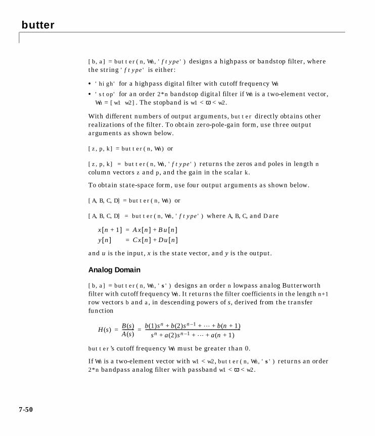
butter
7-50
[b,a] = butter(n,Wn,'ftype') designs a highpass or bandstop filter, wherethe string 'ftype' is either:
• 'high' for a highpass digital filter with cutoff frequency Wn
• 'stop' for an order 2*n bandstop digital filter if Wn is a two-element vector,Wn = [w1 w2]. The stopband is w1 < ω < w2.
With different numbers of output arguments, butter directly obtains otherrealizations of the filter. To obtain zero-pole-gain form, use three outputarguments as shown below.
[z,p,k] = butter(n,Wn) or
[z,p,k] = butter(n,Wn,'ftype') returns the zeros and poles in length ncolumn vectors z and p, and the gain in the scalar k.
To obtain state-space form, use four output arguments as shown below.
[A,B,C,D] = butter(n,Wn) or
[A,B,C,D] = butter(n,Wn,'ftype') where A, B, C, and D are
and u is the input, x is the state vector, and y is the output.
Analog Domain
[b,a] = butter(n,Wn,'s') designs an order n lowpass analog Butterworthfilter with cutoff frequency Wn. It returns the filter coefficients in the length n+1row vectors b and a, in descending powers of s, derived from the transferfunction
butter’s cutoff frequency Wn must be greater than 0.
If Wn is a two-element vector with w1 < w2, butter(n,Wn,'s') returns an order2*n bandpass analog filter with passband w1 < ω < w2.
x n 1+[ ] Ax n[ ] Bu n[ ]+=
y n[ ] Cx n[ ] Du n[ ]+=
H s( )B s( )A s( )----------- b 1( )sn b 2( )sn 1– b n 1+( )+ + +
sn a 2( )sn 1– a n 1+( )+ + +-------------------------------------------------------------------------------------= =

butter
7-51
[b,a] = butter(n,Wn,'ftype','s') designs a highpass or bandstop filter.
With different numbers of output arguments, butter directly obtains otherrealizations of the analog filter. To obtain zero-pole-gain form, use three outputarguments as shown below.
[z,p,k] = butter(n,Wn,'s') or
[z,p,k] = butter(n,Wn,'ftype','s') returns the zeros and poles in lengthn or 2*n column vectors z and p and the gain in the scalar k.
To obtain state-space form, use four output arguments as shown below.
[A,B,C,D] = butter(n,Wn,'s') or
[A,B,C,D] = butter(n,Wn,'ftype','s') where A, B, C, and D are
and u is the input, x is the state vector, and y is the output.
Examples Example 1For data sampled at 1000 Hz, design a 9th-order highpass Butterworth filterwith cutoff frequency of 300 Hz.
[b,a] = butter(9,300/500,'high');
The filter’s frequency response is
freqz(b,a,128,1000)
x· Ax Bu+=
y Cx Du+=
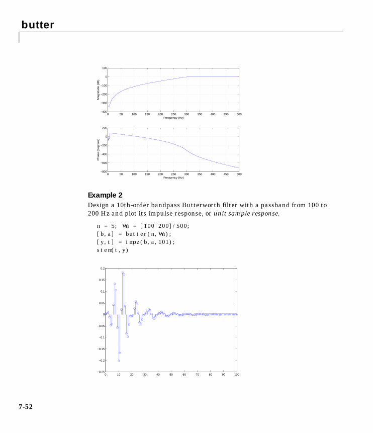
butter
7-52
Example 2Design a 10th-order bandpass Butterworth filter with a passband from 100 to200 Hz and plot its impulse response, or unit sample response.
n = 5; Wn = [100 200]/500;[b,a] = butter(n,Wn);[y,t] = impz(b,a,101);stem(t,y)
0 50 100 150 200 250 300 350 400 450 500−800
−600
−400
−200
0
200
Frequency (Hz)
Pha
se (
degr
ees)
0 50 100 150 200 250 300 350 400 450 500−400
−300
−200
−100
0
100
Frequency (Hz)
Mag
nitu
de (
dB)
0 10 20 30 40 50 60 70 80 90 100−0.25
−0.2
−0.15
−0.1
−0.05
0
0.05
0.1
0.15
0.2

butter
7-53
Limitations For high order filters, the state-space form is the most numerically accurate,followed by the zero-pole-gain form. The transfer function coefficient form isthe least accurate; numerical problems can arise for filter orders as low as 15.
Algorithm butter uses a five-step algorithm:
1 It finds the lowpass analog prototype poles, zeros, and gain using the buttapfunction.
2 It converts the poles, zeros, and gain into state-space form.
3 It transforms the lowpass filter into a bandpass, highpass, or bandstop filterwith desired cutoff frequencies, using a state-space transformation.
4 For digital filter design, butter uses bilinear to convert the analog filterinto a digital filter through a bilinear transformation with frequencyprewarping. Careful frequency adjustment guarantees that the analogfilters and the digital filters will have the same frequency responsemagnitude at Wn or w1 and w2.
5 It converts the state-space filter back to transfer function or zero-pole-gainform, as required.
See Also besself Bessel analog filter design.
buttap Butterworth analog lowpass filter prototype.
buttord Calculate the order of a Butterworth filter.
cheby1 Chebyshev type I filter design (passband ripple).
cheby2 Chebyshev type II filter design (stopband ripple).
ellip Elliptic (Cauer) filter design.
maxflat Generalized Butterworth filter design.
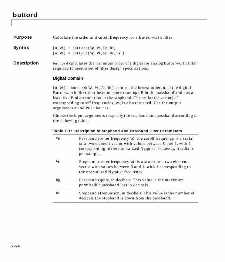
buttord
7-54
7buttordPurpose Calculate the order and cutoff frequency for a Butterworth filter.
Syntax [n,Wn] = buttord(Wp,Ws,Rp,Rs)[n,Wn] = buttord(Wp,Ws,Rp,Rs,'s')
Description buttord calculates the minimum order of a digital or analog Butterworth filterrequired to meet a set of filter design specifications.
Digital Domain
[n,Wn] = buttord(Wp,Ws,Rp,Rs) returns the lowest order, n, of the digitalButterworth filter that loses no more than Rp dB in the passband and has atleast Rs dB of attenuation in the stopband. The scalar (or vector) ofcorresponding cutoff frequencies, Wn, is also returned. Use the outputarguments n and Wn in butter.
Choose the input arguments to specify the stopband and passband according tothe following table.
Table 7-1: Description of Stopband and Passband Filter Parameters
Wp Passband corner frequency Wp, the cutoff frequency, is a scalaror a two-element vector with values between 0 and 1, with 1corresponding to the normalized Nyquist frequency, π radiansper sample.
Ws Stopband corner frequency Ws, is a scalar or a two-elementvector with values between 0 and 1, with 1 corresponding tothe normalized Nyquist frequency.
Rp Passband ripple, in decibels. This value is the maximumpermissible passband loss in decibels.
Rs Stopband attenuation, in decibels. This value is the number ofdecibels the stopband is down from the passband.
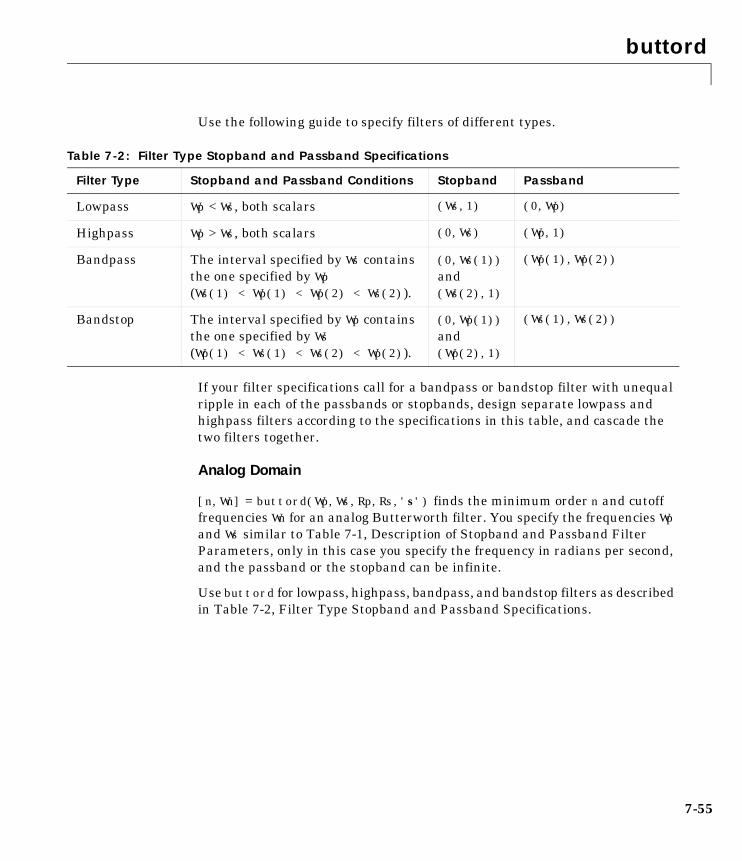
buttord
7-55
Use the following guide to specify filters of different types.
If your filter specifications call for a bandpass or bandstop filter with unequalripple in each of the passbands or stopbands, design separate lowpass andhighpass filters according to the specifications in this table, and cascade thetwo filters together.
Analog Domain
[n,Wn] = buttord(Wp,Ws,Rp,Rs,'s') finds the minimum order n and cutofffrequencies Wn for an analog Butterworth filter. You specify the frequencies Wpand Ws similar to Table 7-1, Description of Stopband and Passband FilterParameters, only in this case you specify the frequency in radians per second,and the passband or the stopband can be infinite.
Use buttord for lowpass, highpass, bandpass, and bandstop filters as describedin Table 7-2, Filter Type Stopband and Passband Specifications.
Table 7-2: Filter Type Stopband and Passband Specifications
Filter Type Stopband and Passband Conditions Stopband Passband
Lowpass Wp < Ws, both scalars (Ws,1) (0,Wp)
Highpass Wp > Ws, both scalars (0,Ws) (Wp,1)
Bandpass The interval specified by Ws containsthe one specified by Wp(Ws(1) < Wp(1) < Wp(2) < Ws(2)).
(0,Ws(1))and(Ws(2),1)
(Wp(1),Wp(2))
Bandstop The interval specified by Wp containsthe one specified by Ws(Wp(1) < Ws(1) < Ws(2) < Wp(2)).
(0,Wp(1))and(Wp(2),1)
(Ws(1),Ws(2))

buttord
7-56
Examples Example 1For data sampled at 1000 Hz, design a lowpass filter with less than 3 dB ofripple in the passband, defined from 0 to 40 Hz, and at least 60 dB ofattenuation in the stopband, defined from 150 Hz to the Nyquist frequency(500 Hz). Plot the filter’s frequency response.
Wp = 40/500; Ws = 150/500;[n,Wn] = buttord(Wp,Ws,3,60)
n = 5Wn = 0.0810
[b,a] = butter(n,Wn);freqz(b,a,512,1000); title('n=5 Butterworth Lowpass Filter')
0 50 100 150 200 250 300 350 400 450 500−500
−400
−300
−200
−100
0
Frequency (Hz)
Ph
ase
(d
eg
ree
s)
0 50 100 150 200 250 300 350 400 450 500−400
−300
−200
−100
0
100
Frequency (Hz)
Ma
gn
itud
e (
dB
)
n=5 Butterworth Lowpass Filter
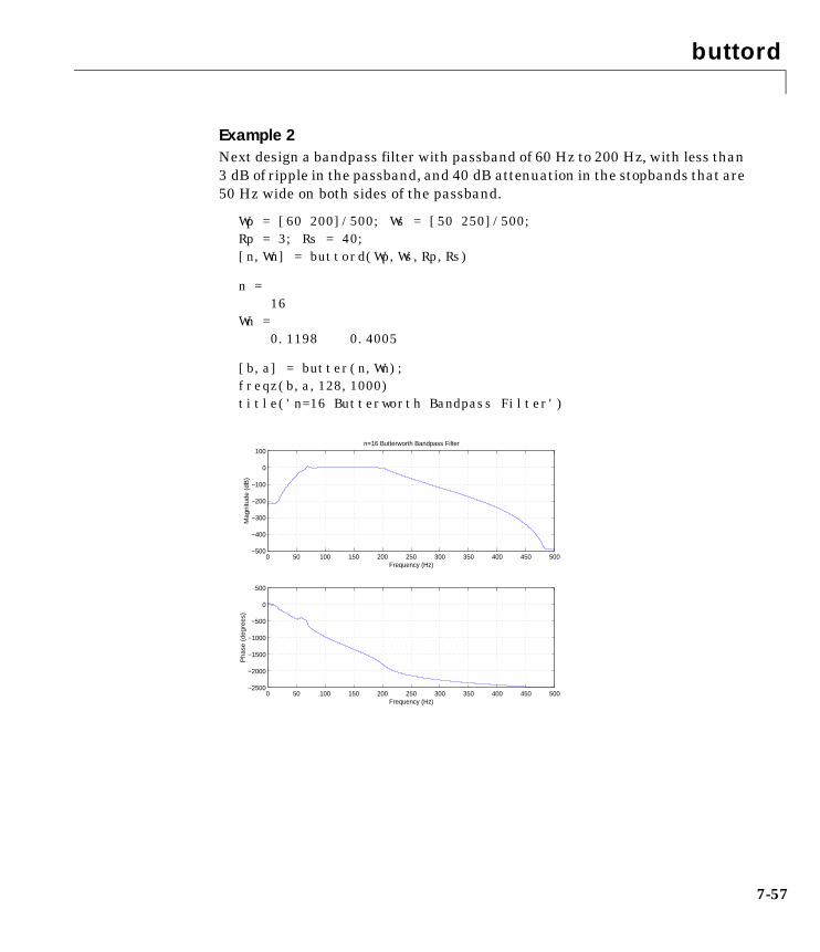
buttord
7-57
Example 2Next design a bandpass filter with passband of 60 Hz to 200 Hz, with less than3 dB of ripple in the passband, and 40 dB attenuation in the stopbands that are50 Hz wide on both sides of the passband.
Wp = [60 200]/500; Ws = [50 250]/500;Rp = 3; Rs = 40;[n,Wn] = buttord(Wp,Ws,Rp,Rs)
n = 16Wn = 0.1198 0.4005
[b,a] = butter(n,Wn);freqz(b,a,128,1000)title('n=16 Butterworth Bandpass Filter')
0 50 100 150 200 250 300 350 400 450 500−2500
−2000
−1500
−1000
−500
0
500
Frequency (Hz)
Ph
ase
(d
eg
ree
s)
0 50 100 150 200 250 300 350 400 450 500−500
−400
−300
−200
−100
0
100
Frequency (Hz)
Ma
gn
itud
e (
dB
)
n=16 Butterworth Bandpass Filter

buttord
7-58
Algorithm buttord’s order prediction formula is described in [1]. It operates in the analogdomain for both analog and digital cases. For the digital case, it converts thefrequency parameters to the s-domain before estimating the order and naturalfrequency, and then converts back to the z-domain.
buttord initially develops a lowpass filter prototype by transforming thepassband frequencies of the desired filter to 1 rad/s (for lowpass and highpassfilters) and to -1 and 1 rad/s (for bandpass and bandstop filters). It thencomputes the minimum order required for a lowpass filter to meet the stopbandspecification.
See Also
References [1] Rabiner, L.R., and B. Gold. Theory and Application of Digital SignalProcessing. Englewood Cliffs, NJ: Prentice-Hall, 1975. Pg. 227.
butter Design a Butterworth analog or digital filter.
cheb1ord Calculate the order for a Chebyshev type I filter.
cheb2ord Calculate the order for a Chebyshev type II filter.
ellipord Calculate the order for an elliptic filter.
kaiserord Estimate Kaiser window FIR filter parameters.
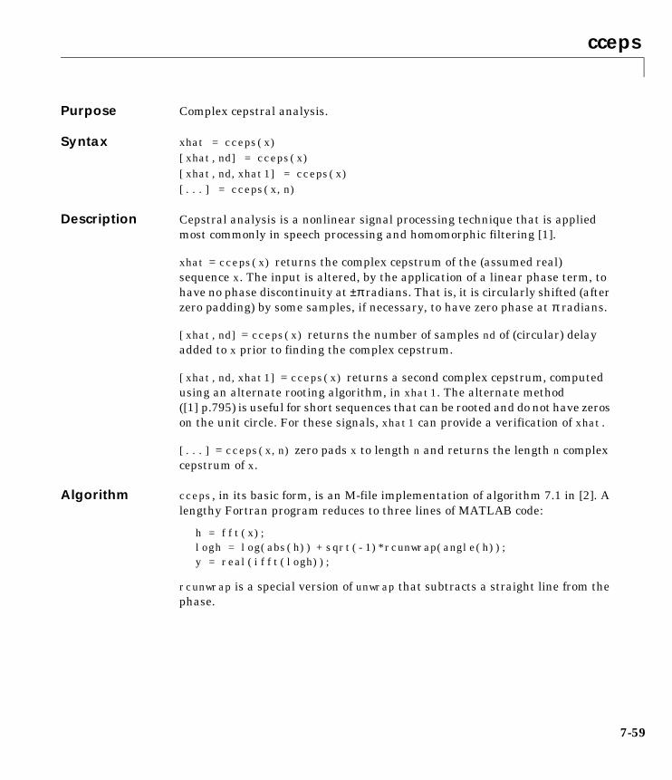
cceps
7-59
7ccepsPurpose Complex cepstral analysis.
Syntax xhat = cceps(x)[xhat,nd] = cceps(x)[xhat,nd,xhat1] = cceps(x)[...] = cceps(x,n)
Description Cepstral analysis is a nonlinear signal processing technique that is appliedmost commonly in speech processing and homomorphic filtering [1].
xhat = cceps(x) returns the complex cepstrum of the (assumed real)sequence x. The input is altered, by the application of a linear phase term, tohave no phase discontinuity at ±π radians. That is, it is circularly shifted (afterzero padding) by some samples, if necessary, to have zero phase at π radians.
[xhat,nd] = cceps(x) returns the number of samples nd of (circular) delayadded to x prior to finding the complex cepstrum.
[xhat,nd,xhat1] = cceps(x) returns a second complex cepstrum, computedusing an alternate rooting algorithm, in xhat1. The alternate method([1] p.795) is useful for short sequences that can be rooted and do not have zeroson the unit circle. For these signals, xhat1 can provide a verification of xhat.
[...] = cceps(x,n) zero pads x to length n and returns the length n complexcepstrum of x.
Algorithm cceps, in its basic form, is an M-file implementation of algorithm 7.1 in [2]. Alengthy Fortran program reduces to three lines of MATLAB code:
h = fft(x);logh = log(abs(h)) + sqrt(-1)*rcunwrap(angle(h));y = real(ifft(logh));
rcunwrap is a special version of unwrap that subtracts a straight line from thephase.

cceps
7-60
See Also
References [1] Oppenheim, A.V., and R.W. Schafer. Discrete-Time Signal Processing.Englewood Cliffs, NJ: Prentice-Hall, 1989.
[2] IEEE. Programs for Digital Signal Processing. IEEE Press. New York: JohnWiley & Sons, 1979.
icceps Inverse complex cepstrum.
hilbert Hilbert transform.
rceps Real cepstrum and minimum phase reconstruction.
unwrap Unwrap phase angles.

cell2sos
7-61
7cell2sosPurpose Convert a cell array for second-order sections to a second-order section matrix.
Syntax m = cell2sos(c)
Description m = cell2sos(c) changes a 1-by-L cell array c consisting of 1-by-2 cell arraysinto an L-by-6 second-order section matrix m. Matrix m takes the same form asthe matrix generated by tf2sos. You can use m = cell2sos(c) to invert theresults of c = sos2cell(m).
c must be a cell array of the form
c = b1 a1 b2 a2 ... bL aL
where both bi and ai are row vectors of at most length 3, and i = 1, 2, ..., L. Theresulting matrix m is given by
m = [b1 a1;b2 a2; ... ;bL aL]
See Also sos2cell Convert second-order section matrices to cell arrays.
tf2sos Convert transfer functions to second-order sections.

cheb1ap
7-62
7cheb1apPurpose Chebyshev type I analog lowpass filter prototype.
Syntax [z,p,k] = cheb1ap(n,Rp)
Description [z,p,k] = cheb1ap(n,Rp) returns the poles and gain of an order n Chebyshevtype I analog lowpass filter prototype with Rp dB of ripple in the passband. Thefunction returns the poles in the length n column vector p and the gain inscalar k. z is an empty matrix, because there are no zeros. The transferfunction is
Chebyshev type I filters are equiripple in the passband and monotonic in thestopband. The poles are evenly spaced about an ellipse in the left half plane.The Chebyshev type I cutoff frequency is set to 1.0 for a normalized result.This is the frequency at which the passband ends and the filter has magnituderesponse of 10-Rp/20.
See Also
References [1] Parks, T.W., and C.S. Burrus. Digital Filter Design. New York: John Wiley& Sons, 1987. Chapter 7.
H s( )z s( )p s( )---------- k
s p 1( )–( ) s p 2( )–( ) s p n( )–( )--------------------------------------------------------------------------------= =
ω0
besselap Bessel analog lowpass filter prototype.
buttap Butterworth analog and digital filter design.
cheb2ap Chebyshev type I analog lowpass filter prototype.
cheby1 Chebyshev type I filter design (passband ripple).
ellipap Elliptic analog lowpass filter prototype.
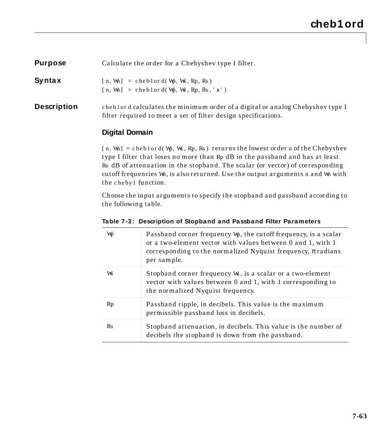
cheb1ord
7-63
7cheb1ordPurpose Calculate the order for a Chebyshev type I filter.
Syntax [n,Wn] = cheb1ord(Wp,Ws,Rp,Rs)[n,Wn] = cheb1ord(Wp,Ws,Rp,Rs,'s')
Description cheb1ord calculates the minimum order of a digital or analog Chebyshev type Ifilter required to meet a set of filter design specifications.
Digital Domain
[n,Wn] = cheb1ord(Wp,Ws,Rp,Rs) returns the lowest order n of the Chebyshevtype I filter that loses no more than Rp dB in the passband and has at leastRs dB of attenuation in the stopband. The scalar (or vector) of correspondingcutoff frequencies Wn, is also returned. Use the output arguments n and Wn withthe cheby1 function.
Choose the input arguments to specify the stopband and passband according tothe following table.
Table 7-3: Description of Stopband and Passband Filter Parameters
Wp Passband corner frequency Wp, the cutoff frequency, is a scalaror a two-element vector with values between 0 and 1, with 1corresponding to the normalized Nyquist frequency, π radiansper sample.
Ws Stopband corner frequency Ws, is a scalar or a two-elementvector with values between 0 and 1, with 1 corresponding tothe normalized Nyquist frequency.
Rp Passband ripple, in decibels. This value is the maximumpermissible passband loss in decibels.
Rs Stopband attenuation, in decibels. This value is the number ofdecibels the stopband is down from the passband.
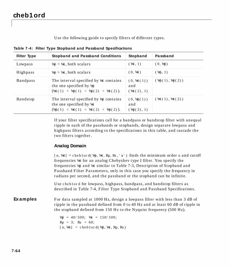
cheb1ord
7-64
Use the following guide to specify filters of different types.
If your filter specifications call for a bandpass or bandstop filter with unequalripple in each of the passbands or stopbands, design separate lowpass andhighpass filters according to the specifications in this table, and cascade thetwo filters together.
Analog Domain
[n,Wn] = cheb1ord(Wp,Ws,Rp,Rs,'s') finds the minimum order n and cutofffrequencies Wn for an analog Chebyshev type I filter. You specify thefrequencies Wp and Ws similar to Table 7-3, Description of Stopband andPassband Filter Parameters, only in this case you specify the frequency inradians per second, and the passband or the stopband can be infinite.
Use cheb1ord for lowpass, highpass, bandpass, and bandstop filters asdescribed in Table 7-4, Filter Type Stopband and Passband Specifications.
Examples For data sampled at 1000 Hz, design a lowpass filter with less than 3 dB ofripple in the passband defined from 0 to 40 Hz and at least 60 dB of ripple inthe stopband defined from 150 Hz to the Nyquist frequency (500 Hz).
Wp = 40/500; Ws = 150/500;Rp = 3; Rs = 60;[n,Wn] = cheb1ord(Wp,Ws,Rp,Rs)
Table 7-4: Filter Type Stopband and Passband Specifications
Filter Type Stopband and Passband Conditions Stopband Passband
Lowpass Wp < Ws, both scalars (Ws,1) (0,Wp)
Highpass Wp > Ws, both scalars (0,Ws) (Wp,1)
Bandpass The interval specified by Ws containsthe one specified by Wp(Ws(1) < Wp(1) < Wp(2) < Ws(2)).
(0,Ws(1))and(Ws(2),1)
(Wp(1),Wp(2))
Bandstop The interval specified by Wp containsthe one specified by Ws(Wp(1) < Ws(1) < Ws(2) < Wp(2)).
(0,Wp(1))and(Wp(2),1)
(Ws(1),Ws(2))
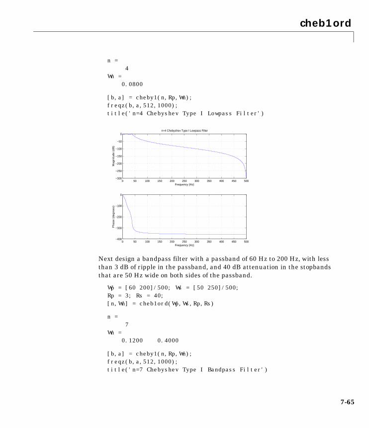
cheb1ord
7-65
n = 4Wn = 0.0800
[b,a] = cheby1(n,Rp,Wn);freqz(b,a,512,1000); title('n=4 Chebyshev Type I Lowpass Filter')
Next design a bandpass filter with a passband of 60 Hz to 200 Hz, with lessthan 3 dB of ripple in the passband, and 40 dB attenuation in the stopbandsthat are 50 Hz wide on both sides of the passband.
Wp = [60 200]/500; Ws = [50 250]/500;Rp = 3; Rs = 40;[n,Wn] = cheb1ord(Wp,Ws,Rp,Rs)
n = 7Wn = 0.1200 0.4000
[b,a] = cheby1(n,Rp,Wn);freqz(b,a,512,1000);title('n=7 Chebyshev Type I Bandpass Filter')
0 50 100 150 200 250 300 350 400 450 500−400
−300
−200
−100
0
Frequency (Hz)
Ph
ase
(d
eg
ree
s)
0 50 100 150 200 250 300 350 400 450 500−300
−250
−200
−150
−100
−50
0
Frequency (Hz)
Ma
gn
itud
e (
dB
)
n=4 Chebyshev Type I Lowpass Filter

cheb1ord
7-66
Algorithm cheb1ord uses the Chebyshev lowpass filter order prediction formula describedin [1]. The function performs its calculations in the analog domain for bothanalog and digital cases. For the digital case, it converts the frequencyparameters to the s-domain before the order and natural frequency estimationprocess, and then converts them back to the z-domain.
cheb1ord initially develops a lowpass filter prototype by transforming thepassband frequencies of the desired filter to 1 rad/s (for low- or highpass filters)or to -1 and 1 rad/s (for bandpass or bandstop filters). It then computes theminimum order required for a lowpass filter to meet the stopband specification.
See Also
References [1] Rabiner, L.R., and B. Gold. Theory and Application of Digital SignalProcessing. Englewood Cliffs, NJ: Prentice-Hall, 1975. Pg. 241.
0 50 100 150 200 250 300 350 400 450 500−1500
−1000
−500
0
500
Frequency (Hz)
Ph
ase
(d
eg
ree
s)
0 50 100 150 200 250 300 350 400 450 500−500
−400
−300
−200
−100
0
Frequency (Hz)
Ma
gn
itud
e (
dB
)
n=7 Chebyshev Type I Bandpass Filter
buttord Calculate the order for a Butterworth filter.
cheby1 Design a Chebyshev type I filter (passband ripple).
cheb2ord Calculate the order for a Chebyshev type II filter.
ellipord Calculate the order for an elliptic filter.
kaiserord Estimate Kaiser window FIR filter parameters.
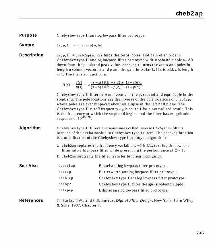
cheb2ap
7-67
7cheb2apPurpose Chebyshev type II analog lowpass filter prototype.
Syntax [z,p,k] = cheb2ap(n,Rs)
Description [z,p,k] = cheb2ap(n,Rs) finds the zeros, poles, and gain of an order nChebyshev type II analog lowpass filter prototype with stopband ripple Rs dBdown from the passband peak value. cheb2ap returns the zeros and poles inlength n column vectors z and p and the gain in scalar k. If n is odd, z is lengthn-1. The transfer function is
Chebyshev type II filters are monotonic in the passband and equiripple in thestopband. The pole locations are the inverse of the pole locations of cheb1ap,whose poles are evenly spaced about an ellipse in the left half plane. TheChebyshev type II cutoff frequency ω0 is set to 1 for a normalized result. Thisis the frequency at which the stopband begins and the filter has magnituderesponse of 10-Rs/20.
Algorithm Chebyshev type II filters are sometimes called inverse Chebyshev filtersbecause of their relationship to Chebyshev type I filters. The cheb2ap functionis a modification of the Chebyshev type I prototype algorithm:
1 cheb2ap replaces the frequency variable ω with 1/ω, turning the lowpassfilter into a highpass filter while preserving the performance at ω = 1.
2 cheb2ap subtracts the filter transfer function from unity.
See Also
References [1] Parks, T.W., and C.S. Burrus. Digital Filter Design. New York: John Wiley& Sons, 1987. Chapter 7.
H s( )z s( )p s( )---------- k s z 1( )–( ) s z 2( )–( ) s z n( )–( )
s p 1( )–( ) s p 2( )–( ) s p n( )–( )--------------------------------------------------------------------------------= =
besselap Bessel analog lowpass filter prototype.
buttap Butterworth analog lowpass filter prototype.
cheb1ap Chebyshev type I analog lowpass filter prototype.
cheby2 Chebyshev type II filter design (stopband ripple).
ellipap Elliptic analog lowpass filter prototype.
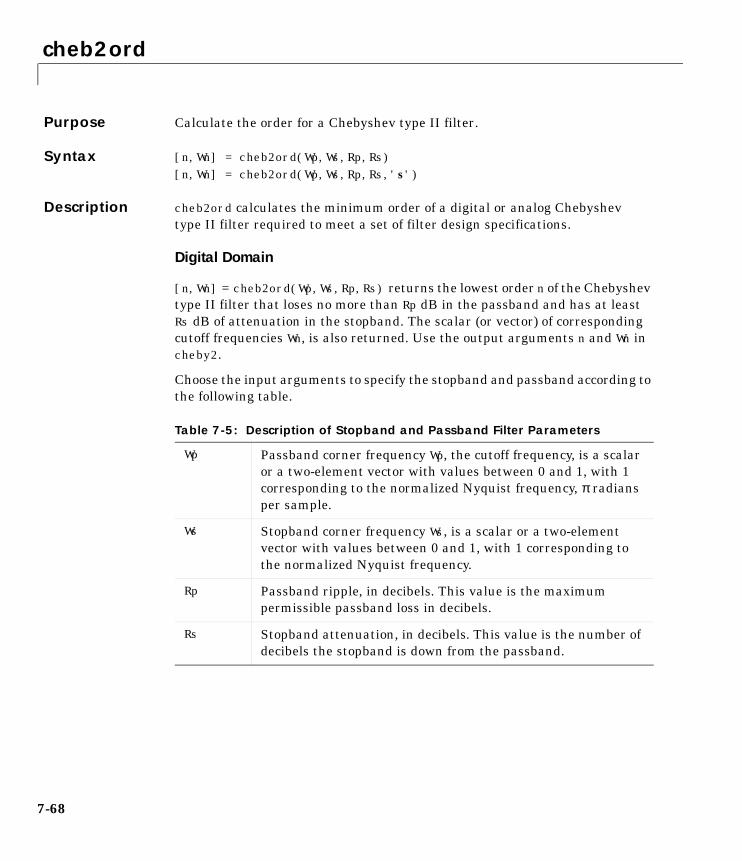
cheb2ord
7-68
7cheb2ordPurpose Calculate the order for a Chebyshev type II filter.
Syntax [n,Wn] = cheb2ord(Wp,Ws,Rp,Rs)[n,Wn] = cheb2ord(Wp,Ws,Rp,Rs,'s')
Description cheb2ord calculates the minimum order of a digital or analog Chebyshevtype II filter required to meet a set of filter design specifications.
Digital Domain
[n,Wn] = cheb2ord(Wp,Ws,Rp,Rs) returns the lowest order n of the Chebyshevtype II filter that loses no more than Rp dB in the passband and has at leastRs dB of attenuation in the stopband. The scalar (or vector) of correspondingcutoff frequencies Wn, is also returned. Use the output arguments n and Wn incheby2.
Choose the input arguments to specify the stopband and passband according tothe following table.
Table 7-5: Description of Stopband and Passband Filter Parameters
Wp Passband corner frequency Wp, the cutoff frequency, is a scalaror a two-element vector with values between 0 and 1, with 1corresponding to the normalized Nyquist frequency, π radiansper sample.
Ws Stopband corner frequency Ws, is a scalar or a two-elementvector with values between 0 and 1, with 1 corresponding tothe normalized Nyquist frequency.
Rp Passband ripple, in decibels. This value is the maximumpermissible passband loss in decibels.
Rs Stopband attenuation, in decibels. This value is the number ofdecibels the stopband is down from the passband.

cheb2ord
7-69
Use the following guide to specify filters of different types.
If your filter specifications call for a bandpass or bandstop filter with unequalripple in each of the passbands or stopbands, design separate lowpass andhighpass filters according to the specifications in this table, and cascade thetwo filters together.
Analog Domain
[n,Wn] = cheb2ord(Wp,Ws,Rp,Rs,'s') finds the minimum order n and cutofffrequencies Wn for an analog Chebyshev type II filter. You specify thefrequencies Wp and Ws similar to Table 7-5, Description of Stopband andPassband Filter Parameters, only in this case you specify the frequency inradians per second, and the passband or the stopband can be infinite.
Use cheb2ord for lowpass, highpass, bandpass, and bandstop filters asdescribed in Table 7-6, Filter Type Stopband and Passband Specifications.
Table 7-6: Filter Type Stopband and Passband Specifications
Filter Type Stopband and Passband Conditions Stopband Passband
Lowpass Wp < Ws, both scalars (Ws,1) (0,Wp)
Highpass Wp > Ws, both scalars (0,Ws) (Wp,1)
Bandpass The interval specified by Ws containsthe one specified by Wp(Ws(1) < Wp(1) < Wp(2) < Ws(2)).
(0,Ws(1))and(Ws(2),1)
(Wp(1),Wp(2))
Bandstop The interval specified by Wp containsthe one specified by Ws(Wp(1) < Ws(1) < Ws(2) < Wp(2)).
(0,Wp(1))and(Wp(2),1)
(Ws(1),Ws(2))
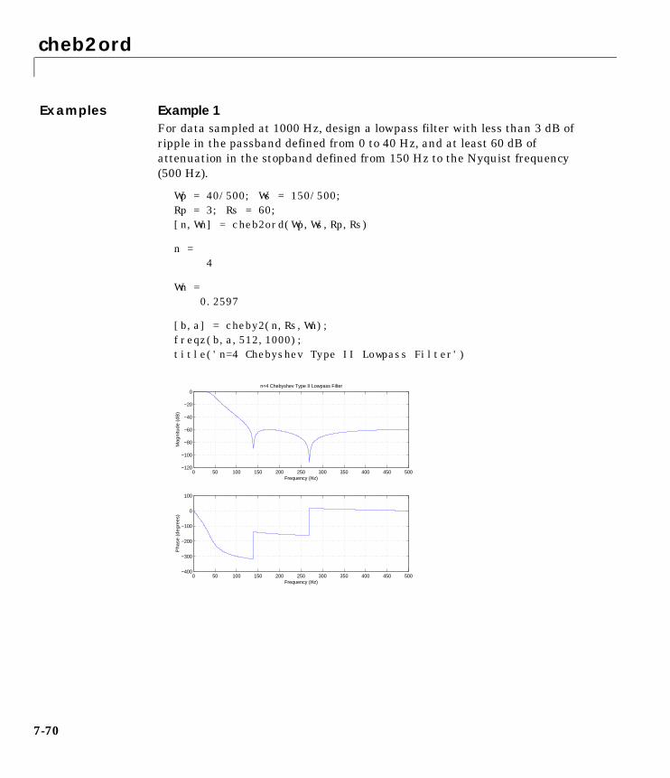
cheb2ord
7-70
Examples Example 1For data sampled at 1000 Hz, design a lowpass filter with less than 3 dB ofripple in the passband defined from 0 to 40 Hz, and at least 60 dB ofattenuation in the stopband defined from 150 Hz to the Nyquist frequency(500 Hz).
Wp = 40/500; Ws = 150/500;Rp = 3; Rs = 60;[n,Wn] = cheb2ord(Wp,Ws,Rp,Rs)
n = 4
Wn = 0.2597
[b,a] = cheby2(n,Rs,Wn);freqz(b,a,512,1000); title('n=4 Chebyshev Type II Lowpass Filter')
0 50 100 150 200 250 300 350 400 450 500−400
−300
−200
−100
0
100
Frequency (Hz)
Ph
ase
(d
eg
ree
s)
0 50 100 150 200 250 300 350 400 450 500−120
−100
−80
−60
−40
−20
0
Frequency (Hz)
Ma
gn
itud
e (
dB
)
n=4 Chebyshev Type II Lowpass Filter
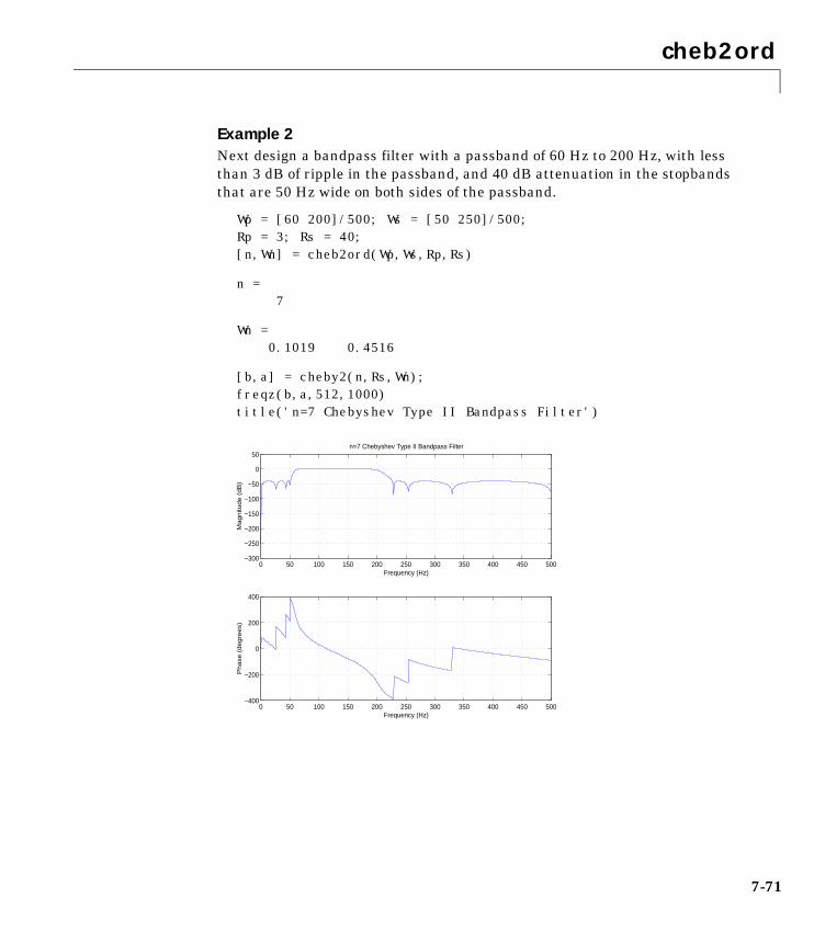
cheb2ord
7-71
Example 2Next design a bandpass filter with a passband of 60 Hz to 200 Hz, with lessthan 3 dB of ripple in the passband, and 40 dB attenuation in the stopbandsthat are 50 Hz wide on both sides of the passband.
Wp = [60 200]/500; Ws = [50 250]/500;Rp = 3; Rs = 40;[n,Wn] = cheb2ord(Wp,Ws,Rp,Rs)
n = 7
Wn = 0.1019 0.4516
[b,a] = cheby2(n,Rs,Wn);freqz(b,a,512,1000)title('n=7 Chebyshev Type II Bandpass Filter')
0 50 100 150 200 250 300 350 400 450 500−400
−200
0
200
400
Frequency (Hz)
Ph
ase
(d
eg
ree
s)
0 50 100 150 200 250 300 350 400 450 500−300
−250
−200
−150
−100
−50
0
50
Frequency (Hz)
Ma
gn
itud
e (
dB
)
n=7 Chebyshev Type II Bandpass Filter

cheb2ord
7-72
Algorithm cheb2ord uses the Chebyshev lowpass filter order prediction formula describedin [1]. The function performs its calculations in the analog domain for bothanalog and digital cases. For the digital case, it converts the frequencyparameters to the s-domain before the order and natural frequency estimationprocess, and then converts them back to the z-domain.
cheb2ord initially develops a lowpass filter prototype by transforming thestopband frequencies of the desired filter to 1 rad/s (for low- and highpassfilters) and to -1 and 1 rad/s (for bandpass and bandstop filters). It thencomputes the minimum order required for a lowpass filter to meet thepassband specification.
See Also
References [1] Rabiner, L.R., and B. Gold. Theory and Application of Digital SignalProcessing. Englewood Cliffs, NJ: Prentice-Hall, 1975. Pg. 241.
buttord Calculate the order for a Butterworth filter.
cheb1ord Calculate the order for a Chebyshev type I filter.
cheby2 Design a Chebyshev type II filter (stopband ripple).
ellipord Calculate the order for an elliptic filter.
kaiserord Estimate Kaiser window FIR filter parameters.
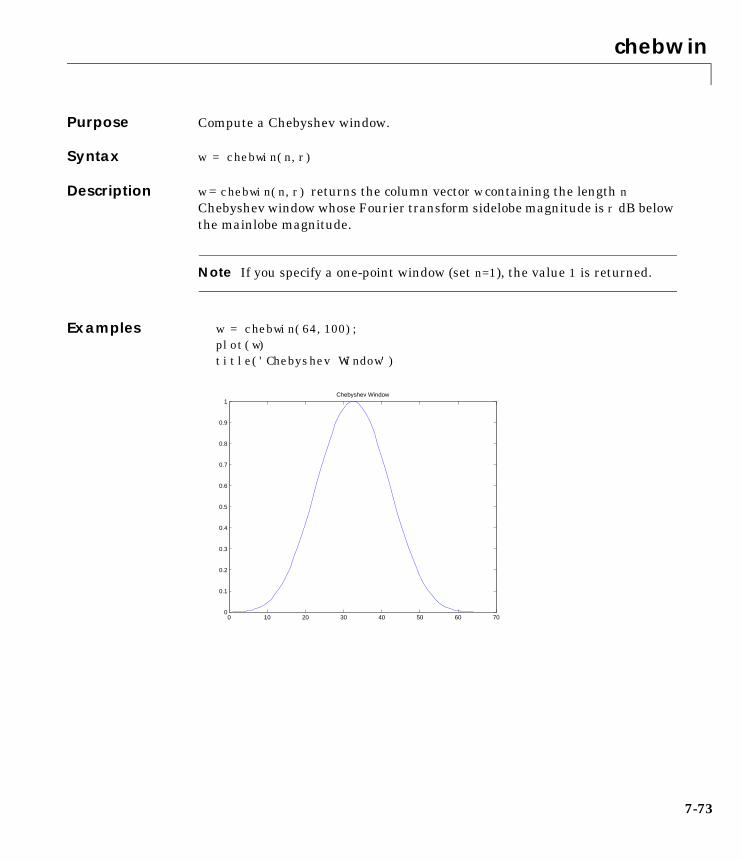
chebwin
7-73
7chebwinPurpose Compute a Chebyshev window.
Syntax w = chebwin(n,r)
Description w = chebwin(n,r) returns the column vector w containing the length nChebyshev window whose Fourier transform sidelobe magnitude is r dB belowthe mainlobe magnitude.
Note If you specify a one-point window (set n=1), the value 1 is returned.
Examples w = chebwin(64,100);plot(w)title('Chebyshev Window')
0 10 20 30 40 50 60 700
0.1
0.2
0.3
0.4
0.5
0.6
0.7
0.8
0.9
1Chebyshev Window

chebwin
7-74
See Also
References [1] IEEE. Programs for Digital Signal Processing. IEEE Press. New York: JohnWiley & Sons, 1979. Program 5.2.
bartlett Compute a Bartlett window.
blackman Compute a Blackman window.
boxcar Compute a rectangular window.
hamming Compute a Hamming window.
hann Compute a Hann window.
kaiser Compute a Kaiser window.
triang Compute a triangular window.

cheby1
7-75
7cheby1Purpose Chebyshev type I filter design (passband ripple).
Syntax [b,a] = cheby1(n,Rp,Wn)[b,a] = cheby1(n,Rp,Wn,'ftype')[b,a] = cheby1(n,Rp,Wn,'s')[b,a] = cheby1(n,Rp,Wn,'ftype','s')[z,p,k] = cheby1(...)[A,B,C,D] = cheby1(...)
Description cheby1 designs lowpass, bandpass, highpass, and bandstop digital and analogChebyshev type I filters. Chebyshev type I filters are equiripple in thepassband and monotonic in the stopband. Type I filters roll off faster thantype II filters, but at the expense of greater deviation from unity in thepassband.
Digital Domain
[b,a] = cheby1(n,Rp,Wn) designs an order n lowpass digital Chebyshev filterwith cutoff frequency Wn and Rp dB of ripple in the passband. It returns thefilter coefficients in the length n+1 row vectors b and a, with coefficients indescending powers of z.
Cutoff frequency is the frequency at which the magnitude response of the filteris equal to -Rp dB. For cheby1, the cutoff frequency Wn is a number between 0and 1, where 1 corresponds to the Nyquist frequency, π radians per sample.Smaller values of passband ripple Rp lead to wider transition widths (shallowerrolloff characteristics).
If Wn is a two-element vector, Wn = [w1 w2], cheby1 returns an order 2*nbandpass filter with passband w1 < < w2.
H z( )B z( )A z( )----------- b 1( ) b 2( )z 1– b n 1+( )z n–+ + +
1 a 2( )z 1– a n 1+( )z n–+ + +------------------------------------------------------------------------------------= =
ω

cheby1
7-76
[b,a] = cheby1(n,Rp,Wn,'ftype') designs a highpass or bandstop filter,where the string 'ftype' is either:
• 'high' for a highpass digital filter with cutoff frequency Wn
• 'stop' for an order 2*n bandstop digital filter if Wn is a two-element vector,Wn = [w1 w2]
The stopband is w1 < ω < w2.
With different numbers of output arguments, cheby1 directly obtains otherrealizations of the filter. To obtain zero-pole-gain form, use three outputarguments as shown below.
[z,p,k] = cheby1(n,Rp,Wn) or
[z,p,k] = cheby1(n,Rp,Wn,'ftype') returns the zeros and poles in length ncolumn vectors z and p and the gain in the scalar k.
To obtain state-space form, use four output arguments as shown below.
[A,B,C,D] = cheby1(n,Rp,Wn) or
[A,B,C,D] = cheby1(n,Rp,Wn,'ftype') where A, B, C, and D are
and u is the input, x is the state vector, and y is the output.
Analog Domain
[b,a] = cheby1(n,Rp,Wn,'s') designs an order n lowpass analog Chebyshevtype I filter with cutoff frequency Wn. It returns the filter coefficients in lengthn+1 row vectors b and a, in descending powers of s, derived from the transferfunction
Cutoff frequency is the frequency at which the magnitude response of the filteris -Rp dB. For cheby1, the cutoff frequency Wn must be greater than 0.
x n 1+[ ] Ax n[ ] Bu n[ ]+=
y n[ ] Cx n[ ] Du n[ ]+=
H s( )B s( )A s( )----------- b 1( )sn b 2( )sn 1– b n 1+( )+ + +
sn a 2( )sn 1– a n 1+( )+ + +-------------------------------------------------------------------------------------= =
cheby1
7-77
If Wn is a two-element vector Wn = [w1 w2] with w1 < w2, thencheby1(n,Rp,Wn,'s') returns an order 2*n bandpass analog filter withpassband w1 < ω < w2.
[b,a] = cheby1(n,Rp,Wn,'ftype','s') designs a highpass or bandstop filter.
You can supply different numbers of output arguments for cheby1 to directlyobtain other realizations of the analog filter. To obtain zero-pole-gain form, usethree output arguments as shown below.
[z,p,k] = cheby1(n,Rp,Wn,'s') or
[z,p,k] = cheby1(n,Rp,Wn,'ftype','s') returns the zeros and poles inlength n or 2*n column vectors z and p and the gain in the scalar k.
To obtain state-space form, use four output arguments as shown below.
[A,B,C,D] = cheby1(n,Rp,Wn,'s') or
[A,B,C,D] = cheby1(n,Rp,Wn,'ftype','s') where A, B, C, and D are definedas
and u is the input, x is the state vector, and y is the output.
Examples For data sampled at 1000 Hz, design a 9th-order lowpass Chebyshev type Ifilter with 0.5 dB of ripple in the passband and a cutoff frequency of 300 Hz.
[b,a] = cheby1(9,0.5,300/500);
The frequency response of the filter is
freqz(b,a,512,1000)
x· Ax Bu+=
y Cx Du+=

cheby1
7-78
Design a 10th-order bandpass Chebyshev type I filter with a passband from100 to 200 Hz and plot its impulse response.
n = 10; Rp = 0.5;Wn = [100 200]/500;[b,a] = cheby1(n,Rp,Wn);[y,t] = impz(b,a,101); stem(t,y)
0 50 100 150 200 250 300 350 400 450 500-1000
-800
-600
-400
-200
0
Frequency (Hertz)
Pha
se (
degr
ees)
0 50 100 150 200 250 300 350 400 450 500-300
-200
-100
0
100
Frequency (Hertz)
Mag
nitu
de R
espo
nse
(dB
)
n = 9 Chebyshev Type I Lowpass Filter
0 10 20 30 40 50 60 70 80 90 100-0.2
-0.15
-0.1
-0.05
0
0.05
0.1
0.15Impulse Response of n = 10 Chebyshev Type I Filter

cheby1
7-79
Limitations For high order filters, the state-space form is the most numerically accurate,followed by the zero-pole-gain form. The transfer function form is the leastaccurate; numerical problems can arise for filter orders as low as 15.
Algorithm cheby1 uses a five-step algorithm:
1 It finds the lowpass analog prototype poles, zeros, and gain using thecheb1ap function.
2 It converts the poles, zeros, and gain into state-space form.
3 It transforms the lowpass filter into a bandpass, highpass, or bandstop filterwith desired cutoff frequencies, using a state-space transformation.
4 For digital filter design, cheby1 uses bilinear to convert the analog filterinto a digital filter through a bilinear transformation with frequencyprewarping. Careful frequency adjustment guarantees that the analogfilters and the digital filters will have the same frequency responsemagnitude at Wn or w1 and w2.
5 It converts the state-space filter back to transfer function or zero-pole-gainform, as required.
See Also besself Bessel analog filter design.
butter Butterworth analog and digital filter design.
cheb1ap Chebyshev type I analog lowpass filter prototype.
cheb1ord Calculate the order of a Chebyshev type I filter.
cheby2 Chebyshev type II filter design (stopband ripple).
ellip Elliptic (Cauer) filter design.

cheby2
7-80
7cheby2Purpose Chebyshev type II filter design (stopband ripple).
Syntax [b,a] = cheby2(n,Rs,Wn)[b,a] = cheby2(n,Rs,Wn,'ftype')[b,a] = cheby2(n,Rs,Wn,'s')[b,a] = cheby2(n,Rs,Wn,'ftype','s')[z,p,k] = cheby2(...)[A,B,C,D] = cheby2(...)
Description cheby2 designs lowpass, highpass, bandpass, and bandstop digital and analogChebyshev type II filters. Chebyshev type II filters are monotonic in thepassband and equiripple in the stopband. Type II filters do not roll off as fastas type I filters, but are free of passband ripple.
Digital Domain
[b,a] = cheby2(n,Rs,Wn) designs an order n lowpass digital Chebyshev typeII filter with cutoff frequency Wn and stopband ripple Rs dB down from the peakpassband value. It returns the filter coefficients in the length n+1 row vectorsb and a, with coefficients in descending powers of z.
Cutoff frequency is the beginning of the stopband, where the magnituderesponse of the filter is equal to -Rs dB. For cheby2, the normalized cutofffrequency Wn is a number between 0 and 1, where 1 corresponds to the Nyquistfrequency. Larger values of stopband attenuation Rs lead to wider transitionwidths (shallower rolloff characteristics).
If Wn is a two-element vector, Wn = [w1 w2], cheby2 returns an order 2*nbandpass filter with passband w1 < ω < w2.
[b,a] = cheby2(n,Rs,Wn,'ftype') designs a highpass or bandstop filter,where the string 'ftype' is either:
• 'high' for a highpass digital filter with cutoff frequency Wn
• 'stop' for an order 2*n bandstop digital filter if Wn is a two-element vector,Wn = [w1 w2]. The stopband is w1 < ω < w2.
H z( )B z( )A z( )----------- b 1( ) b 2( )z 1– b n 1+( )z n–+ + +
1 a 2( )z 1– a n 1+( )z n–+ + +------------------------------------------------------------------------------------= =
cheby2
7-81
With different numbers of output arguments, cheby2 directly obtains otherrealizations of the filter. To obtain zero-pole-gain form, use three outputarguments as shown below.
[z,p,k] = cheby2(n,Rs,Wn) or
[z,p,k] = cheby2(n,Rs,Wn,'ftype') returns the zeros and poles in length ncolumn vectors z and p and the gain in the scalar k.
To obtain state-space form, use four output arguments as shown below.
[A,B,C,D] = cheby2(n,Rs,Wn) or
[A,B,C,D] = cheby2(n,Rs,Wn,'ftype') where A, B, C, and D are
and u is the input, x is the state vector, and y is the output.
Analog Domain
[b,a] = cheby2(n,Rs,Wn,'s') designs an order n lowpass analog Chebyshevtype II filter with cutoff frequency Wn. It returns the filter coefficients in thelength n+1 row vectors b and a, with coefficients in descending powers of s,derived from the transfer function.
Cutoff frequency is the frequency at which the magnitude response of the filteris equal to -Rs dB. For cheby2, the cutoff frequency Wn must be greater than 0.
If Wn is a two-element vector Wn = [w1 w2] with w1 < w2, thencheby2(n,Rs,Wn,'s') returns an order 2*n bandpass analog filter withpassband w1 < ω < w2.
[b,a] = cheby2(n,Rs,Wn,'ftype','s') designs a highpass or bandstop filter.
With different numbers of output arguments, cheby2 directly obtains otherrealizations of the analog filter. To obtain zero-pole-gain form, use three outputarguments as shown below.
x n 1+[ ] Ax n[ ] Bu n[ ]+=
y n[ ] Cx n[ ] Du n[ ]+=
H s( )B s( )A s( )----------- b 1( )sn b 2( )sn 1– b n 1+( )+ + +
sn a 2( )sn 1– a n 1+( )+ + +-------------------------------------------------------------------------------------= =
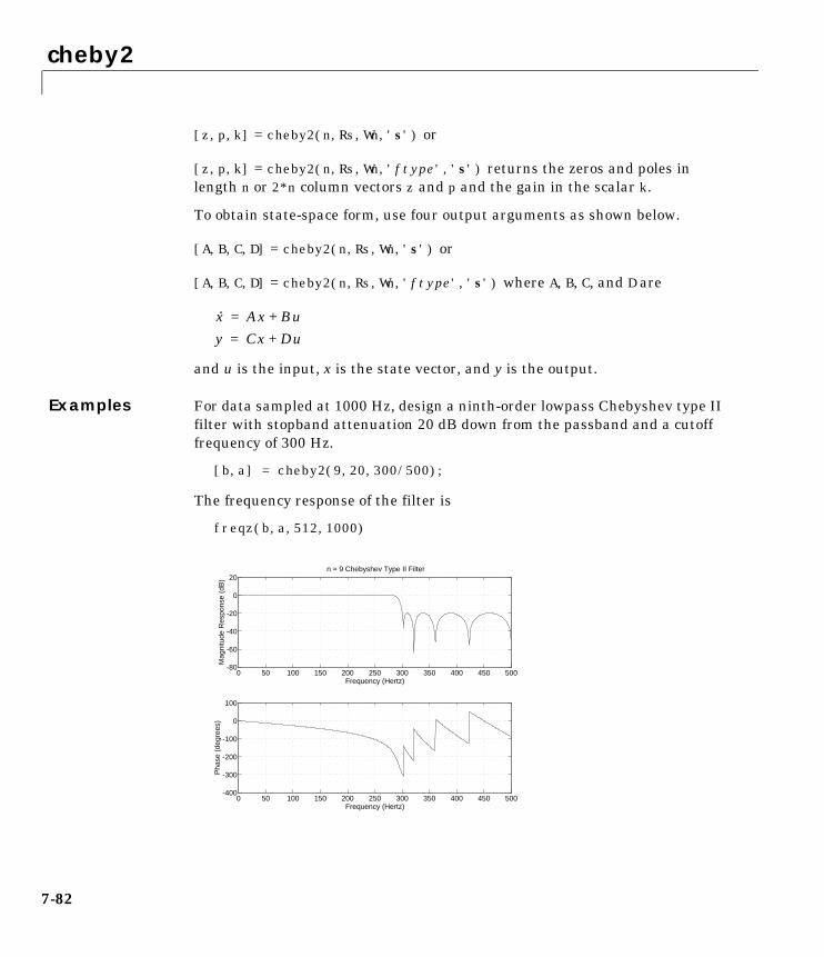
cheby2
7-82
[z,p,k] = cheby2(n,Rs,Wn,'s') or
[z,p,k] = cheby2(n,Rs,Wn,'ftype','s') returns the zeros and poles inlength n or 2*n column vectors z and p and the gain in the scalar k.
To obtain state-space form, use four output arguments as shown below.
[A,B,C,D] = cheby2(n,Rs,Wn,'s') or
[A,B,C,D] = cheby2(n,Rs,Wn,'ftype','s') where A, B, C, and D are
and u is the input, x is the state vector, and y is the output.
Examples For data sampled at 1000 Hz, design a ninth-order lowpass Chebyshev type IIfilter with stopband attenuation 20 dB down from the passband and a cutofffrequency of 300 Hz.
[b,a] = cheby2(9,20,300/500);
The frequency response of the filter is
freqz(b,a,512,1000)
x· Ax Bu+=
y Cx Du+=
0 50 100 150 200 250 300 350 400 450 500-400
-300
-200
-100
0
100
Frequency (Hertz)
Pha
se (
degr
ees)
0 50 100 150 200 250 300 350 400 450 500-80
-60
-40
-20
0
20
Frequency (Hertz)
Mag
nitu
de R
espo
nse
(dB
)
n = 9 Chebyshev Type II Filter

cheby2
7-83
Design a fifth-order bandpass Chebyshev type II filter with passband from 100to 200 Hz and plot the impulse response of the filter.
n = 5; r = 20;Wn = [100 200]/500;[b,a] = cheby2(n,r,Wn);[y,t] = impz(b,a,101); stem(t,y)
Limitations For high order filters, the state-space form is the most numerically accurate,followed by the zero-pole-gain form. The transfer function coefficient form isthe least accurate; numerical problems can arise for filter orders as low as 15.
Algorithm cheby2 uses a five-step algorithm:
1 It finds the lowpass analog prototype poles, zeros, and gain using thecheb2ap function.
2 It converts poles, zeros, and gain into state-space form.
3 It transforms the lowpass filter into a bandpass, highpass, or bandstop filterwith desired cutoff frequencies, using a state-space transformation.
4 For digital filter design, cheby2 uses bilinear to convert the analog filterinto a digital filter through a bilinear transformation with frequencyprewarping. Careful frequency adjustment guarantees that the analog
0 10 20 30 40 50 60 70 80 90 100-0.2
-0.15
-0.1
-0.05
0
0.05
0.1
0.15
0.2Impulse Response of n = 5 Chebyshev Type II Filter
cheby2
7-84
filters and the digital filters will have the same frequency responsemagnitude at Wn or w1 and w2.
5 It converts the state-space filter back to transfer function or zero-pole-gainform, as required.
See Also besself Bessel analog filter design.
butter Butterworth analog and digital filter design.
cheb2ap Chebyshev type II analog lowpass filter prototype.
cheb2ord Calculate the order of a Chebyshev type II filter.
cheby1 Chebyshev type I filter design (passband ripple).
ellip Elliptic (Cauer) filter design.
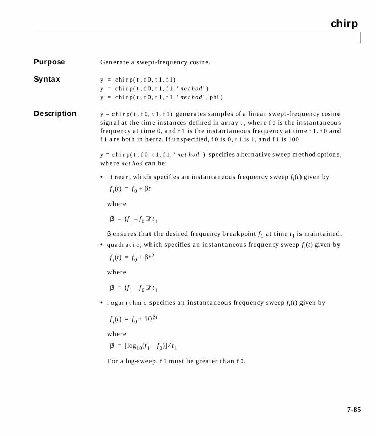
chirp
7-85
7chirpPurpose Generate a swept-frequency cosine.
Syntax y = chirp(t,f0,t1,f1)y = chirp(t,f0,t1,f1,'method')y = chirp(t,f0,t1,f1,'method',phi)
Description y = chirp(t,f0,t1,f1) generates samples of a linear swept-frequency cosinesignal at the time instances defined in array t, where f0 is the instantaneousfrequency at time 0, and f1 is the instantaneous frequency at time t1. f0 andf1 are both in hertz. If unspecified, f0 is 0, t1 is 1, and f1 is 100.
y = chirp(t,f0,t1,f1,'method') specifies alternative sweep method options,where method can be:
• linear, which specifies an instantaneous frequency sweep fi(t) given by
where
β ensures that the desired frequency breakpoint f1 at time t1 is maintained.
• quadratic, which specifies an instantaneous frequency sweep fi(t) given by
where
• logarithmic specifies an instantaneous frequency sweep fi(t) given by
where
For a log-sweep, f1 must be greater than f0.
fi t( ) f0 βt+=
β f1 f0–( ) t1⁄=
fi t( ) f0 βt2+=
β f1 f0–( ) t1⁄=
fi t( ) f0 10βt+=
β log10 f1 f0–( )[ ] t1⁄=
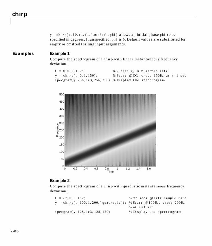
chirp
7-86
y = chirp(t,f0,t1,f1,'method',phi) allows an initial phase phi to bespecified in degrees. If unspecified, phi is 0. Default values are substituted forempty or omitted trailing input arguments.
Examples Example 1Compute the spectrogram of a chirp with linear instantaneous frequencydeviation.
t = 0:0.001:2; % 2 secs @ 1kHz sample ratey = chirp(t,0,1,150); % Start @ DC, cross 150Hz at t=1 secspecgram(y,256,1e3,256,250) % Display the spectrogram
Example 2Compute the spectrogram of a chirp with quadratic instantaneous frequencydeviation.
t = -2:0.001:2; % ±2 secs @ 1kHz sample ratey = chirp(t,100,1,200,'quadratic'); % Start @ 100Hz, cross 200Hz
% at t=1 secspecgram(y,128,1e3,128,120) % Display the spectrogram
Time
Fre
quen
cy
0 0.2 0.4 0.6 0.8 1 1.2 1.4 1.60
50
100
150
200
250
300
350
400
450
500
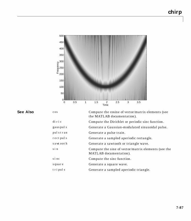
chirp
7-87
See Also
Time
Fre
quen
cy
0 0.5 1 1.5 2 2.5 3 3.50
50
100
150
200
250
300
350
400
450
500
cos Compute the cosine of vector/matrix elements (seethe MATLAB documentation).
diric Compute the Dirichlet or periodic sinc function.
gauspuls Generate a Gaussian-modulated sinusoidal pulse.
pulstran Generate a pulse train.
rectpuls Generate a sampled aperiodic rectangle.
sawtooth Generate a sawtooth or triangle wave.
sin Compute the sine of vector/matrix elements (see theMATLAB documentation).
sinc Compute the sinc function.
square Generate a square wave.
tripuls Generate a sampled aperiodic triangle.
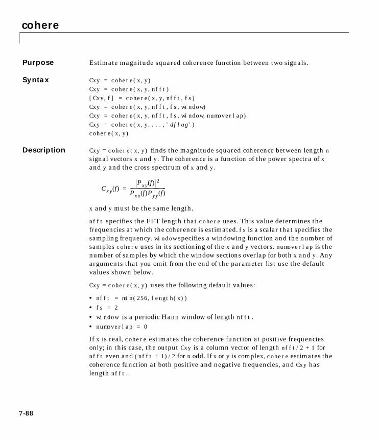
cohere
7-88
7coherePurpose Estimate magnitude squared coherence function between two signals.
Syntax Cxy = cohere(x,y)Cxy = cohere(x,y,nfft)[Cxy,f] = cohere(x,y,nfft,fs)Cxy = cohere(x,y,nfft,fs,window)Cxy = cohere(x,y,nfft,fs,window,numoverlap)Cxy = cohere(x,y,...,'dflag')cohere(x,y)
Description Cxy = cohere(x,y) finds the magnitude squared coherence between length nsignal vectors x and y. The coherence is a function of the power spectra of xand y and the cross spectrum of x and y.
x and y must be the same length.
nfft specifies the FFT length that cohere uses. This value determines thefrequencies at which the coherence is estimated. fs is a scalar that specifies thesampling frequency. window specifies a windowing function and the number ofsamples cohere uses in its sectioning of the x and y vectors. numoverlap is thenumber of samples by which the window sections overlap for both x and y. Anyarguments that you omit from the end of the parameter list use the defaultvalues shown below.
Cxy = cohere(x,y) uses the following default values:
• nfft = min(256,length(x))
• fs = 2
• window is a periodic Hann window of length nfft.• numoverlap = 0
If x is real, cohere estimates the coherence function at positive frequenciesonly; in this case, the output Cxy is a column vector of length nfft/2 + 1 fornfft even and (nfft + 1)/2 for n odd. If x or y is complex, cohere estimates thecoherence function at both positive and negative frequencies, and Cxy haslength nfft.
Cxy f( )Pxy f( ) 2
Pxx f( )Pyy f( )-------------------------------=
cohere
7-89
Cxy = cohere(x,y,nfft) uses the FFT length nfft in estimating the powerspectrum for x. Specify nfft as a power of 2 for fastest execution.
Cxy = cohere(x,y,nfft,fs) returns a vector f of frequencies at which thefunction evaluates the coherence. fs is the sampling frequency. f is the samesize as Cxy, so plot(f,Cxy) plots the coherence function versus properly scaledfrequency. fs has no effect on the output Cxy; it is a frequency scalingmultiplier.
cohere(x,y,nfft,fs,window) specifies a windowing function and the numberof samples per section of the vectors x and y. If you supply a scalar for window,cohere uses a Hann window of that length. The length of the window must beless than or equal to nfft; cohere zero pads the sections if the window lengthexceeds nfft.
cohere(x,y,nfft,fs,window,numoverlap) overlaps the sections of x bynumoverlap samples.
You can use the empty matrix [] to specify the default value for any inputargument except x or y. For example,
cohere(x,y,[],[],kaiser(128,5));
uses 256 as the value for nfft and 2 as the value for fs.
cohere(x,y,...,'dflag') specifies a detrend option, where 'dflag' is:
• 'linear', to remove the best straight-line fit from the prewindowed sectionsof x and y
• 'mean', to remove the mean from the prewindowed sections of x and y
• 'none', for no detrending (default)
The 'dflag' parameter must appear last in the list of input arguments. cohererecognizes a 'dflag' string no matter how many intermediate arguments areomitted.
cohere with no output arguments plots the coherence estimate versusfrequency in the current figure window.
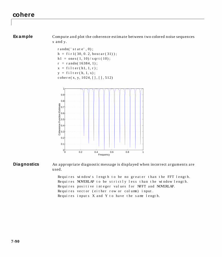
cohere
7-90
Example Compute and plot the coherence estimate between two colored noise sequencesx and y.
randn('state',0);h = fir1(30,0.2,boxcar(31));h1 = ones(1,10)/sqrt(10);r = randn(16384,1);x = filter(h1,1,r);y = filter(h,1,x);cohere(x,y,1024,[],[],512)
Diagnostics An appropriate diagnostic message is displayed when incorrect arguments areused.
Requires window's length to be no greater than the FFT length.Requires NOVERLAP to be strictly less than the window length.Requires positive integer values for NFFT and NOVERLAP.Requires vector (either row or column) input.Requires inputs X and Y to have the same length.
0 0.2 0.4 0.6 0.8 10
0.1
0.2
0.3
0.4
0.5
0.6
0.7
0.8
0.9
1
Frequency
Coh
eren
ce F
unct
ion
Est
imat
e
cohere
7-91
Algorithm cohere estimates the magnitude squared coherence function [1] using Welch’smethod of power spectrum estimation (see references [2] and [3]), as follows:
1 It divides the signals x and y into separate overlapping sections, detrendseach section, and multiplies each section by window.
2 It calculates the length nfft fast Fourier transform of each section.
3 It averages the squares of the spectra of the x sections to form Pxx, averagesthe squares of the spectra of the y sections to form Pyy, and averages theproducts of the spectra of the x and y sections to form Pxy. It calculates Cxyby the following formula.
Cxy = abs(Pxy).^2/(Pxx.*Pyy)
See Also
References [1] Kay, S.M. Modern Spectral Estimation. Englewood Cliffs, NJ:Prentice-Hall, 1988. Pg. 454.
[2] Rabiner, L.R., and B. Gold. Theory and Application of Digital SignalProcessing. Englewood Cliffs, NJ: Prentice-Hall, 1975.
[3] Welch, P.D. “The Use of Fast Fourier Transform for the Estimation of PowerSpectra: A Method Based on Time Averaging Over Short, ModifiedPeriodograms.” IEEE Trans. Audio Electroacoust. Vol. AU-15 (June 1967).Pgs. 70-73.
csd Estimate the cross spectral density (CSD) of twosignals.
pwelch Power spectral density estimate using Welch’smethod.
tfe Transfer function estimate from input and output.
conv
7-92
7convPurpose Convolution and polynomial multiplication.
Syntax c = conv(a,b)
Description c = conv(a,b) convolves vectors a and b. The convolution sum is
where N is the maximum sequence length. The series is indexed from n + 1 andk + 1 instead of the usual n and k because MATLAB vectors run from 1 to ninstead of from 0 to n-1.
The conv function is part of the standard MATLAB language.
Example The convolution of a = [1 2 3] and b = [4 5 6] is
c = conv(a,b)
c =4 13 28 27 18
Algorithm The conv function is an M-file that uses the filter primitive. conv computesthe convolution operation as FIR filtering with an appropriate number of zerosappended to the input.
See Also
c n 1+( ) a k 1+( )b n k–( )
k 0=
N 1–
=
conv2 Two-dimensional convolution.
convmtx Convolution matrix.
convn N-dimensional convolution (see the MATLABdocumentation).
deconv Deconvolution and polynomial division.
filter Apply a filter to data.
residuez z-transform partial fraction expansion.
xcorr Cross-correlation function estimate.

conv2
7-93
7conv2Purpose Two-dimensional convolution.
Syntax C = conv2(A,B)C = conv2(A,B,'shape')
Description C = conv2(A,B) computes the two-dimensional convolution of matrices Aand B. If one of these matrices describes a two-dimensional FIR filter, the othermatrix is filtered in two dimensions.
Each dimension of the output matrix C is equal in size to one less than the sumof the corresponding dimensions of the input matrices. When[ma,na] = size(A) and [mb,nb] = size(B),
size(C) = [ma+mb-1,na+nb-1]
C = conv2(A,B,'shape') returns a subsection of the two-dimensionalconvolution with size specified by 'shape', where:
• 'full' returns the full two-dimensional convolution (default)
• 'same' returns the central part of the convolution that is the same size as A
• 'valid' returns only those parts of the convolution that are computedwithout the zero-padded edges. Using this option,size(C) = [ma-mb+1,na-nb+1] when size(A) > size(B)
conv2 executes most quickly when size(A) > size(B).
The conv2 function is part of the standard MATLAB language.
Examples In image processing, the Sobel edge-finding operation is a two-dimensionalconvolution of an input array with the special matrix
s = [1 2 1; 0 0 0; -1 -2 -1];
Given any image, the following code extracts the horizontal edges.
h = conv2(I,s);
The following code extracts the vertical edges first, and then extracts bothhorizontal and vertical edges combined.
v = conv2(I,s');v2 = (sqrt(h.^2 + v.^2))

conv2
7-94
See Also conv Convolution and polynomial multiplication.
convn N-dimensional convolution (see the MATLABdocumentation).
deconv Deconvolution and polynomial division.
filter2 Apply a two-dimensional filter to data.
xcorr Cross-correlation function estimate.
xcorr2 Two-dimensional cross-correlation.

convmtx
7-95
7convmtxPurpose Convolution matrix.
Syntax A = convmtx(c,n)A = convmtx(r,n)
Description A convolution matrix is a matrix, formed from a vector, whose inner productwith another vector is the convolution of the two vectors.
A = convmtx(c,n) where c is a length m column vector returns a matrix A ofsize (m+n-1)-by-n. The product of A and another column vector x of length n isthe convolution of c with x.
A = convmtx(r,n) where r is a length m row vector returns a matrix A of sizen-by-(m+n-1). The product of A and another row vector x of length n is theconvolution of r with x.
Example Generate a simple convolution matrix.
h = [1 2 3 2 1];convmtx(h,7)ans =
1 2 3 2 1 0 0 0 0 0 0 0 1 2 3 2 1 0 0 0 0 0 0 0 1 2 3 2 1 0 0 0 0 0 0 0 1 2 3 2 1 0 0 0 0 0 0 0 1 2 3 2 1 0 0 0 0 0 0 0 1 2 3 2 1 0 0 0 0 0 0 0 1 2 3 2 1
Note that convmtx handles edge conditions by zero padding.
In practice, it is more efficient to compute convolution using
y = conv(c,x)
than by using a convolution matrix.
n = length(x);y = convmtx(c,n)*x
Algorithm convmtx uses the function toeplitz to generate the convolution matrix.

convmtx
7-96
See Also conv Convolution and polynomial multiplication.
convn N-dimensional convolution (see the MATLABdocumentation).
conv2 Two-dimensional convolution.
dftmtx Discrete Fourier transform matrix.
corrcoef
7-97
7corrcoefPurpose Compute the correlation coefficient matrix.
Syntax C = corrcoef(X)C = corrcoef(X,Y)
Description corrcoef returns a matrix of correlation coefficients calculated from an inputmatrix whose rows are observations and whose columns are variables. IfC = cov(X), then corrcoef(X) is the matrix whose element (i, j) is
C = corrcoef(X) is the zeroth lag of the covariance function, that is, thezeroth lag of xcov(x,'coeff') packed into a square array.
C = corrcoef(X,Y) is the same as corrcoef([X Y]); that is, it concatenates Xand Y in the row direction before its computation.
corrcoef removes the mean from each column before calculating the results.See the xcorr function for cross-correlation options.
The corrcoef function is part of the standard MATLAB language.
See Also
corrcoef i j,( )C i j,( )
C i i,( )C j j,( )-----------------------------------=
cov Covariance matrix.
mean Average value (see the MATLAB documentation).
median Median value (see the MATLAB documentation).
std Standard deviation (see the MATLABdocumentation).
xcorr Cross-correlation function estimate.
xcov Cross-covariance function estimate (equal tomean-removed cross-correlation).
corrmtx
7-98
7corrmtxPurpose Compute a data matrix for autocorrelation matrix estimation.
Syntax X = corrmtx(x,m)X = corrmtx(x,m,'method')[X,R] = corrmtx(...)
Description X = corrmtx(x,m) returns an (n+m)-by-(m+1) rectangular Toeplitz matrix X,such that X'X is a (biased) estimate of the autocorrelation matrix for thelength n data vector x.
X = corrmtx(x,m,'method') computes the matrix X according to the methodspecified by the string 'method':
• 'autocorrelation': (default) X is the (n+m)-by-(m+1) rectangular Toeplitzmatrix that generates an autocorrelation estimate for the length n datavector x, derived using prewindowed and postwindowed data, based on anmth order prediction error model.
• 'prewindowed': X is the n-by-(m+1) rectangular Toeplitz matrix thatgenerates an autocorrelation estimate for the length n data vector x, derivedusing prewindowed data, based on an mth order prediction error model.
• 'postwindowed': X is the n-by-(m+1) rectangular Toeplitz matrix thatgenerates an autocorrelation estimate for the length n data vector x, derivedusing postwindowed data, based on an mth order prediction error model.
• 'covariance': X is the (n-m)-by-(m+1) rectangular Toeplitz matrix thatgenerates an autocorrelation estimate for the length n data vector x, derivedusing nonwindowed data, based on an mth order prediction error model.
• 'modified': X is the 2(n-m)-by-(m+1) modified rectangular Toeplitz matrixthat generates an autocorrelation estimate for the length n data vector x,derived using forward and backward prediction error estimates, based on anmth order prediction error model.
[X,R] = corrmtx(...) also returns the (m+1)-by-(m+1) autocorrelation matrixestimate R, calculated as X'*X.
Examples randn('state',1); n=0:99; s=exp(i*pi/2*n)+2*exp(i*pi/4*n)+exp(i*pi/3*n)+randn(1,100); X=corrmtx(s,12,'mod');

corrmtx
7-99
Algorithm The Toeplitz data matrix computed by corrmtx depends on the method youselect. The matrix determined by the autocorrelation (default) method is givenby the following matrix.
In this matrix, m is the same as the input argument m to corrmtx, and n islength(x). Variations of this matrix are used to return the output X of corrmtxfor each method:
• 'autocorrelation': (default) X = X, above.
• 'prewindowed': X is the n-by-(m+1) submatrix of X that is given by theportion of X above the lower gray line.
• 'postwindowed': X is the n-by-(m+1) submatrix of X that is given by theportion of X below the upper gray line.
• 'covariance': X is the (n-m)-by-(m+1) submatrix of X that is given by theportion of X between the two gray lines.
• 'modified': X is the 2(n-m)-by-(m+1) matrix Xmod shown below.
X
x 1( ) 0
x m 1+( ) x1 )
x n m–( ) x m 1+( )
x n( ) x n m–( )
0 x n( )
=
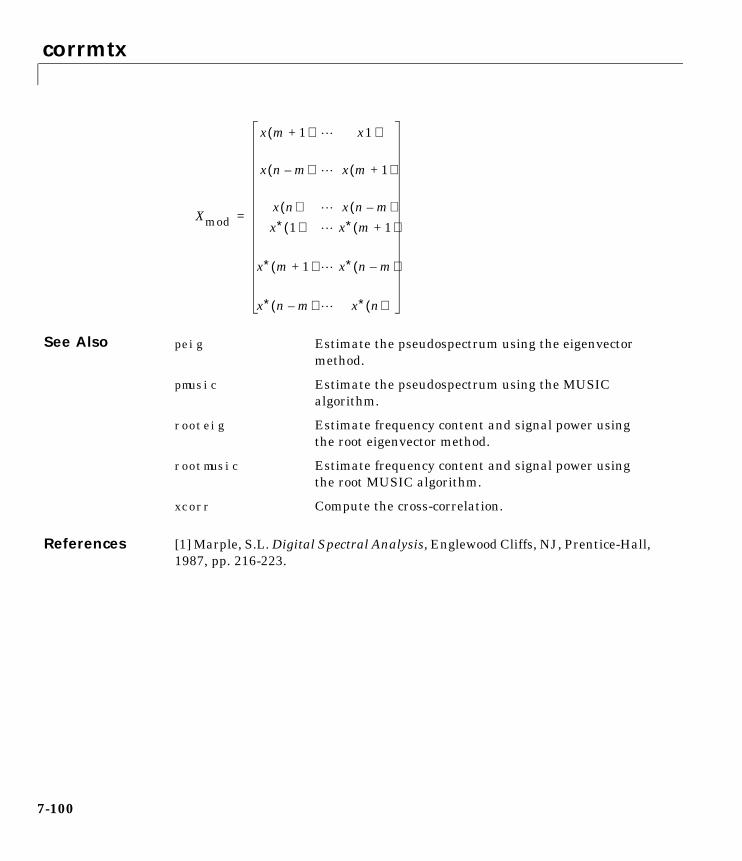
corrmtx
7-100
See Also
References [1] Marple, S.L. Digital Spectral Analysis, Englewood Cliffs, NJ, Prentice-Hall,1987, pp. 216-223.
Xmod
x m 1+( ) x1 )
x n m–( ) x m 1+( )
x n( ) x n m–( )x∗ 1( ) x∗ m 1+( )
x∗ m 1+( ) x∗ n m–( )
x∗ n m–( ) x∗ n( )
=
peig Estimate the pseudospectrum using the eigenvectormethod.
pmusic Estimate the pseudospectrum using the MUSICalgorithm.
rooteig Estimate frequency content and signal power usingthe root eigenvector method.
rootmusic Estimate frequency content and signal power usingthe root MUSIC algorithm.
xcorr Compute the cross-correlation.
cov
7-101
7covPurpose Compute the covariance matrix.
Syntax c = cov(x)c = cov(x,y)
Description cov computes the covariance matrix. If x is a vector, c is a scalar containing thevariance. For an array where each row is an observation and each column avariable, cov(X) is the covariance matrix. diag(cov(X)) is a vector ofvariances for each column, and sqrt(diag(cov(X))) is a vector of standarddeviations.
cov(x) is the zeroth lag of the covariance function, that is, the zeroth lag ofxcov(x)/(n-1) packed into a square array.
cov(x,y) where x and y are column vectors of equal length is equivalent tocov([x y])), that is, it concatenates x and y in the row direction before itscomputation.
cov removes the mean from each column before calculating the results.
The cov function is part of the standard MATLAB language.
Algorithm [n,p] = size(x);x = x-ones(n,1)*(sum(x)/n);y = x'*x/(n-1);
See Also corrcoef Correlation coefficient matrix.
mean Average value (see the MATLAB documentation).
median Median value (see the MATLAB documentation).
std Standard deviation (see the MATLABdocumentation).
xcorr Cross-correlation function estimate.
xcov Cross-covariance function estimate (equal tomean-removed cross-correlation).
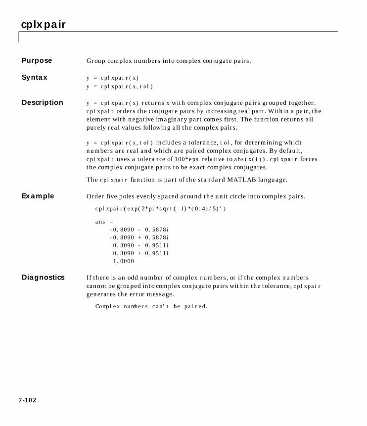
cplxpair
7-102
7cplxpairPurpose Group complex numbers into complex conjugate pairs.
Syntax y = cplxpair(x)y = cplxpair(x,tol)
Description y = cplxpair(x) returns x with complex conjugate pairs grouped together.cplxpair orders the conjugate pairs by increasing real part. Within a pair, theelement with negative imaginary part comes first. The function returns allpurely real values following all the complex pairs.
y = cplxpair(x,tol) includes a tolerance, tol, for determining whichnumbers are real and which are paired complex conjugates. By default,cplxpair uses a tolerance of 100*eps relative to abs(x(i)). cplxpair forcesthe complex conjugate pairs to be exact complex conjugates.
The cplxpair function is part of the standard MATLAB language.
Example Order five poles evenly spaced around the unit circle into complex pairs.
cplxpair(exp(2*pi*sqrt(-1)*(0:4)/5)')
ans =-0.8090 - 0.5878i-0.8090 + 0.5878i0.3090 - 0.9511i0.3090 + 0.9511i1.0000
Diagnostics If there is an odd number of complex numbers, or if the complex numberscannot be grouped into complex conjugate pairs within the tolerance, cplxpairgenerates the error message.
Complex numbers can't be paired.

cremez
7-103
7cremezPurpose Complex and nonlinear-phase equiripple FIR filter design.
Syntax b = cremez(n,f,'fresp')b = cremez(n,f,'fresp',w)b = cremez(n,f,'fresp',p1,p2,...,w)b = cremez(n,f,a,w)b = cremez(...,'sym')b = cremez(...,'skip_stage2')b = cremez(...,'debug')b = cremez(...,lgrid)[b,delta,opt] = cremez(...)
Description cremez allows arbitrary frequency-domain constraints to be specified for thedesign of a possibly complex FIR filter. The Chebyshev (or minimax) filter erroris optimized, producing equiripple FIR filter designs.
b = cremez(n,f,'fresp') returns a length n+1 FIR filter with the bestapproximation to the desired frequency response as returned by functionfresp. f is a vector of frequency band edge pairs, specified in the range -1and 1, where 1 corresponds to the normalized Nyquist frequency. Thefrequencies must be in increasing order, and f must have even length. Thefrequency bands span f(k) to f(k+1) for k odd; the intervals f(k+1) to f(k+2)for k odd are “transition bands” or “don’t care” regions during optimization.
b = cremez(n,f,'fresp',w) uses the real, non-negative weights in vector w toweight the fit in each frequency band. The length of w is half the length of f, sothere is exactly one weight per band.
b = cremez(n,f,'fresp',p1,p2,...,...) supplies optional parametersp1, p2, ..., to the frequency response function fresp. Predefined 'fresp'frequency response functions are included for a number of common filterdesigns, as described below. For all of the predefined frequency responsefunctions, the symmetry option 'sym' defaults to 'even' if no negativefrequencies are contained in f and d = 0; otherwise 'sym' defaults to 'none'.(See the 'sym' option below for details.) For all of the predefined frequencyresponse functions, d specifies a group-delay offset such that the filter response

cremez
7-104
has a group delay of n/2+d in units of the sample interval. Negative valuescreate less delay; positive values create more delay. By default d = 0:
• lowpass, highpass, bandpass, bandstop
These functions share a common syntax, exemplified below by the string'lowpass'.
b = cremez(n,f,'lowpass',...) and
b = cremez(n,f,'lowpass',d,...) design a linear-phase(n/2+d delay) filter.
• multiband designs a linear-phase frequency response filter with arbitraryband amplitudes.
b = cremez(n,f,'multiband',a,...) and
b = cremez(n,f,'multiband',a,d,...) specify vector a containingthe desired amplitudes at the band edges in f. The desired amplitude atfrequencies between pairs of points f(k) and f(k+1) for k odd is the linesegment connecting the points (f(k),a(k)) and (f(k+1),a(k+1)).
• differentiator designs a linear-phase differentiator. For these designs,zero-frequency must be in a transition band, and band weighting is set to beinversely proportional to frequency.
b = cremez(n,f,'differentiator',fs,...) and
b = cremez(n,f,'differentiator',fs,d,...) specify the sample ratefs used to determine the slope of the differentiator response. If omitted, fsdefaults to 1.
• hilbfilt designs a linear-phase Hilbert transform filter response. ForHilbert designs, zero-frequency must be in a transition band.
b = cremez(n,f,'hilbfilt',...) and
b = cremez(N,F,'hilbfilt',d,...) design a linear-phase(n/2+d delay) Hilbert transform filter.
b = cremez(n,f,a,w) is a synonym forb = cremez(n,f,'multiband',a,w).
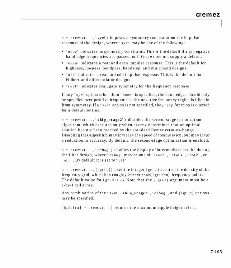
cremez
7-105
b = cremez(...,'sym') imposes a symmetry constraint on the impulseresponse of the design, where 'sym' may be one of the following:
• 'none' indicates no symmetry constraint. This is the default if any negativeband edge frequencies are passed, or if fresp does not supply a default.
• 'even' indicates a real and even impulse response. This is the default forhighpass, lowpass, bandpass, bandstop, and multiband designs.
• 'odd' indicates a real and odd impulse response. This is the default forHilbert and differentiator designs.
• 'real' indicates conjugate symmetry for the frequency response
If any 'sym' option other than 'none' is specified, the band edges should onlybe specified over positive frequencies; the negative frequency region is filled infrom symmetry. If a 'sym' option is not specified, the fresp function is queriedfor a default setting.
b = cremez(...,'skip_stage2') disables the second-stage optimizationalgorithm, which executes only when cremez determines that an optimalsolution has not been reached by the standard Remez error-exchange.Disabling this algorithm may increase the speed of computation, but may incura reduction in accuracy. By default, the second-stage optimization is enabled.
b = cremez(...,'debug') enables the display of intermediate results duringthe filter design, where 'debug' may be one of 'trace', 'plots', 'both', or 'off'. By default it is set to 'off'.
b = cremez(...,lgrid) uses the integer lgrid to control the density of thefrequency grid, which has roughly 2^nextpow2(lgrid*n) frequency points.The default value for lgrid is 25. Note that the lgrid argument must be a1-by-1 cell array.
Any combination of the 'sym', 'skip_stage2', 'debug', and lgrid optionsmay be specified.
[b,delta] = cremez(...) returns the maximum ripple height delta.

cremez
7-106
[b,delta,opt] = cremez(...) returns a structure opt of optional resultscomputed by cremez and contains the following fields.
User-definable functions may be used, instead of the predefined frequencyresponse functions for fresp. The function is called from within cremez usingthe following syntax
[dh,dw] = fresp(n,f,gf,w,p1,p2,...)
where:
• n is the filter order.
• f is the vector of frequency band edges that appear monotonically between -1and 1, where 1 corresponds to the Nyquist frequency.
• gf is a vector of grid points that have been linearly interpolated over eachspecified frequency band by cremez. gf determines the frequency grid atwhich the response function must be evaluated. This is the same datareturned by cremez in the fgrid field of the opt structure.
• w is a vector of real, positive weights, one per band, used during optimization.w is optional in the call to cremez; if not specified, it is set to unity weightingbefore being passed to fresp.
• dh and dw are the desired complex frequency response and band weightvectors, respectively, evaluated at each frequency in grid gf.
• p1, p2, ..., are optional parameters that may be passed to fresp.
opt.fgrid Frequency grid vector used for the filter design optimization
opt.des Desired frequency response for each point in opt.fgrid
opt.wt Weighting for each point in opt.fgrid
opt.H Actual frequency response for each point in opt.fgrid
opt.error Error at each point in opt.fgrid
opt.iextr Vector of indices into opt.fgrid for extremal frequencies
opt.fextr Vector of extremal frequencies
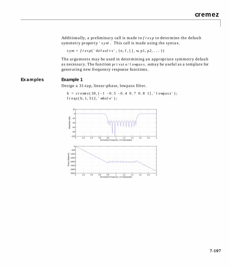
cremez
7-107
Additionally, a preliminary call is made to fresp to determine the defaultsymmetry property 'sym'. This call is made using the syntax.
sym = fresp('defaults',n,f,[],w,p1,p2,...)
The arguments may be used in determining an appropriate symmetry defaultas necessary. The function private/lowpass.m may be useful as a template forgenerating new frequency response functions.
Examples Example 1Design a 31-tap, linear-phase, lowpass filter.
b = cremez(30,[-1 -0.5 -0.4 0.7 0.8 1],'lowpass');freqz(b,1,512,'whole');
0 0.2 0.4 0.6 0.8 1 1.2 1.4 1.6 1.8 2−3500
−3000
−2500
−2000
−1500
−1000
−500
0
Normalized Frequency (×π rad/sample)
Pha
se (
degr
ees)
0 0.2 0.4 0.6 0.8 1 1.2 1.4 1.6 1.8 2−100
−80
−60
−40
−20
0
20
Normalized Frequency (×π rad/sample)
Mag
nitu
de (
dB)
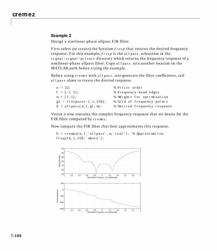
cremez
7-108
Example 2Design a nonlinear-phase allpass FIR filter.
First select (or create) the function fresp that returns the desired frequencyresponse. For this example, fresp is the allpass.m function in thesignal/signal/private directory which returns the frequency response of anonlinear-phase allpass filter. Copy allpass.m to another location on theMATLAB path before trying the example.
Before using cremez with allpass.m to generate the filter coefficients, callallpass alone to create the desired response.
n = 22; % Filter orderf = [-1 1]; % Frequency band edgesw = [1 1]; % Weights for optimizationgf = linspace(-1,1,256); % Grid of frequency points d = allpass(n,f,gf,w); % Desired frequency response
Vector d now contains the complex frequency response that we desire for theFIR filter computed by cremez.
Now compute the FIR filter that best approximates this response.
b = cremez(n,f,'allpass',w,'real'); % Approximationfreqz(b,1,256,'whole');
0 0.2 0.4 0.6 0.8 1 1.2 1.4 1.6 1.8 2−1500
−1000
−500
0
500
Normalized Frequency (×π rad/sample)
Pha
se (
degr
ees)
0 0.2 0.4 0.6 0.8 1 1.2 1.4 1.6 1.8 2−90
−80
−70
−60
−50
−40
−30
Normalized Frequency (×π rad/sample)
Mag
nitu
de (
dB)
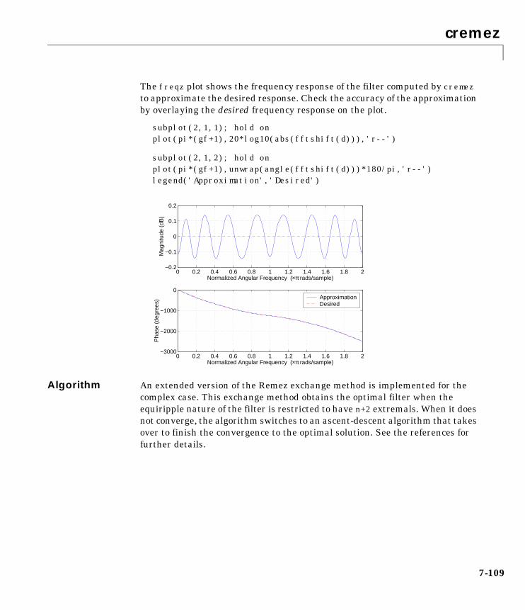
cremez
7-109
The freqz plot shows the frequency response of the filter computed by cremez to approximate the desired response. Check the accuracy of the approximationby overlaying the desired frequency response on the plot.
subplot(2,1,1); hold onplot(pi*(gf+1),20*log10(abs(fftshift(d))),'r--')
subplot(2,1,2); hold onplot(pi*(gf+1),unwrap(angle(fftshift(d)))*180/pi,'r--')legend('Approximation','Desired')
Algorithm An extended version of the Remez exchange method is implemented for thecomplex case. This exchange method obtains the optimal filter when theequiripple nature of the filter is restricted to have n+2 extremals. When it doesnot converge, the algorithm switches to an ascent-descent algorithm that takesover to finish the convergence to the optimal solution. See the references forfurther details.
0 0.2 0.4 0.6 0.8 1 1.2 1.4 1.6 1.8 2−3000
−2000
−1000
0
Normalized Angular Frequency (×π rads/sample)
Pha
se (
degr
ees)
0 0.2 0.4 0.6 0.8 1 1.2 1.4 1.6 1.8 2−0.2
−0.1
0
0.1
0.2
Normalized Angular Frequency (×π rads/sample)
Mag
nitu
de (
dB)
ApproximationDesired
cremez
7-110
See Also
References [1] Karam, L.J., and J.H. McClellan. “Complex Chebyshev Approximation forFIR Filter Design.” IEEE Trans. on Circuits and Systems II. March 1995.Pgs. 207-216.
[2] Karam, L.J. Design of Complex Digital FIR Filters in the Chebyshev Sense.Ph.D. Thesis, Georgia Institute of Technology, March 1995.
[3] Demjanjov, V.F., and V.N. Malozemov. Introduction to Minimax. New York:John Wiley & Sons, 1974.
fir1 FIR filter design using the window method.
fir2 FIR filter design with arbitrary filter shape using thewindow method.
firls Linear phase FIR filter design using theleast-squares method.
remez Parks-McClellan optimal FIR filter design.
csd
7-111
7csdPurpose Estimate the cross spectral density (CSD) of two signals.
Syntax Pxy = csd(x,y)Pxy = csd(x,y,nfft)[Pxy,f] = csd(x,y,nfft,fs)Pxy = csd(x,y,nfft,fs,window)Pxy = csd(x,y,nfft,fs,window,numoverlap)Pxy = csd(x,y,...,'dflag')[Pxy,Pxyc,f] = csd(x,y,nfft,fs,window,numoverlap,p)csd(x,y,...)
Description Pxy = csd(x,y) estimates the cross spectral density of the length n sequencesx and y using the Welch method of spectral estimation. Pxy = csd(x,y) usesthe following default values:
• nfft = min(256,length(x))
• fs = 2
• window is a periodic Hann window of length nfft.
• numoverlap = 0
nfft specifies the FFT length that csd uses. This value determines thefrequencies at which the cross spectrum is estimated. fs is a scalar thatspecifies the sampling frequency. window specifies a windowing function andthe number of samples csd uses in its sectioning of the x and y vectors.numoverlap is the number of samples by which the sections overlap. Anyarguments omitted from the end of the parameter list use the default valuesshown above.
If x and y are real, csd estimates the cross spectral density at positivefrequencies only; in this case, the output Pxy is a column vector of lengthnfft/2 + 1 for nfft even and (nfft + 1)/2 for nfft odd. If x or y is complex,csd estimates the cross spectral density at both positive and negativefrequencies and Pxy has length nfft.
Pxy = csd(x,y,nfft) uses the FFT length nfft in estimating the crossspectral density of x and y. Specify nfft as a power of 2 for fastest execution.
[Pxy,f] = csd(x,y,nfft,fs) returns a vector f of frequencies at which thefunction evaluates the CSD. f is the same size as Pxy, so plot(f,Pxy) plots the
csd
7-112
spectrum versus properly scaled frequency. fs has no effect on the output Pxy;it is a frequency scaling multiplier.
Pxy = csd(x,y,nfft,fs,window) specifies a windowing function and thenumber of samples per section of the x vector. If you supply a scalar for window,csd uses a Hann window of that length. The length of the window must be lessthan or equal to nfft; csd zero pads the sections if the length of the window isless than nfft. csd returns an error if the length of the window is greater thannfft.
Pxy = csd(x,y,nfft,fs,window,numoverlap) overlaps the sections of x and yby numoverlap samples.
You can use the empty matrix [] to specify the default value for any inputargument except x or y. For example,
csd(x,y,[],10000)
is equivalent to
csd(x)
but with a sampling frequency of 10,000 Hz instead of the default of 2 Hz.
Pxy = csd(x,y,...,'dflag') specifies a detrend option, where the string'dflag' is one of the following:
• 'linear', to remove the best straight-line fit from the prewindowed sectionsof x and y
• 'mean', to remove the mean from the prewindowed sections of x and y
• 'none', for no detrending (default)
The dflag parameter must appear last in the list of input arguments. csdrecognizes a dflag string no matter how many intermediate arguments areomitted.
[Pxy,Pxyc,f] = csd(x,y,nfft,fs,window,numoverlap,p) where p is apositive scalar between 0 and 1 returns a vector Pxyc that contains an estimateof the p*100 percent confidence interval for Pxy. Pxyc is a two-column matrixthe same length as Pxy. The interval [Pxyc(:,1),Pxyc(:,2)] covers the true
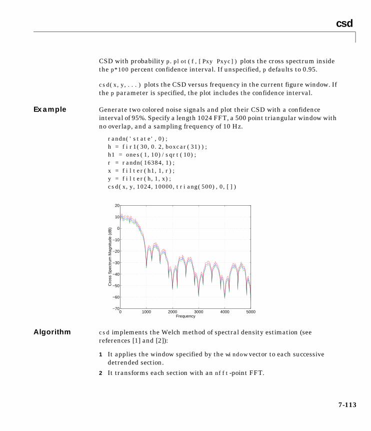
csd
7-113
CSD with probability p. plot(f,[Pxy Pxyc]) plots the cross spectrum insidethe p*100 percent confidence interval. If unspecified, p defaults to 0.95.
csd(x,y,...) plots the CSD versus frequency in the current figure window. Ifthe p parameter is specified, the plot includes the confidence interval.
Example Generate two colored noise signals and plot their CSD with a confidenceinterval of 95%. Specify a length 1024 FFT, a 500 point triangular window withno overlap, and a sampling frequency of 10 Hz.
randn('state',0);h = fir1(30,0.2,boxcar(31));h1 = ones(1,10)/sqrt(10);r = randn(16384,1);x = filter(h1,1,r);y = filter(h,1,x);csd(x,y,1024,10000,triang(500),0,[])
Algorithm csd implements the Welch method of spectral density estimation (seereferences [1] and [2]):
1 It applies the window specified by the window vector to each successivedetrended section.
2 It transforms each section with an nfft-point FFT.
0 1000 2000 3000 4000 5000−70
−60
−50
−40
−30
−20
−10
0
10
20
Frequency
Cro
ss S
pect
rum
Mag
nitu
de (
dB)
csd
7-114
3 It forms the periodogram of each section by scaling the product of thetransform of the y section and the conjugate of the transformed x section.
4 It averages the periodograms of the successive overlapping sections to formPxy, the cross spectral density of x and y.
The number of sections that csd averages is k, where k is
fix((length(x)-numoverlap)/(length(window)-numoverlap))
Diagnostics An appropriate diagnostic message is displayed when incorrect arguments tocsd are used.
Requires window's length to be no greater than the FFT length.Requires NOVERLAP to be strictly less than the window length.Requires positive integer values for NFFT and NOVERLAP.Requires vector (either row or column) input.Requires inputs X and Y to have the same length.Requires confidence parameter to be a scalar between 0 and 1.
See Also
References [1] Rabiner, L.R., and B. Gold. Theory and Application of Digital SignalProcessing. Englewood Cliffs, NJ: Prentice-Hall, 1975. Pgs. 414-419.
[2] Welch, P.D. “The Use of Fast Fourier Transform for the Estimation of PowerSpectra: A Method Based on Time Averaging Over Short, ModifiedPeriodograms.” IEEE Trans. Audio Electroacoust. Vol. AU-15 (June 1967).Pgs. 70-73.
cohere Estimate magnitude squared coherence functionbetween two signals.
pburg Estimate the power spectrum using the Burgmethod.
pmtm Estimate the power spectrum using the multitapermethod (MTM).
pmusic Estimate the pseudospectrum using the MUSICalgorithm.
pwelch Estimate the power spectrum using Welch’s method.
pyulear Estimate the power spectrum using the Yule-Walkerautoregressive method.
tfe Transfer function estimate from input and output.

csd
7-115
[3] Oppenheim, A.V., and R.W. Schafer. Discrete-Time Signal Processing.Englewood Cliffs, NJ: Prentice-Hall, 1989. Pg. 737.
czt
7-116
7cztPurpose Chirp z-transform.
Syntax y = czt(x,m,w,a)y = czt(x)
Description y = czt(x,m,w,a) returns the chirp z-transform of signal x. The chirpz-transform is the z-transform of x along a spiral contour defined by w and a.m is a scalar that specifies the length of the transform, w is the ratio betweenpoints along the z-plane spiral contour of interest, and scalar a is the complexstarting point on that contour. The contour, a spiral or “chirp” in the z-plane, isgiven by
z = a*(w.^-(0:m-1))
y = czt(x) uses the following default values:
• m = length(x)
• w = exp(j*2*pi/m)
• a = 1
With these defaults, czt returns the z-transform of x at m equally spaced pointsaround the unit circle. This is equivalent to the discrete Fourier transform of x,or fft(x). The empty matrix [] specifies the default value for a parameter.
If x is a matrix, czt(x,m,w,a) transforms the columns of x.
Examples Create a random vector x of length 1013 and compute its DFT using czt. Thisis faster than the fft function on the same sequence.
randn('state',0);x = randn(1013,1);y = czt(x);
Use czt to zoom in on a narrow-band section (100 to 150 Hz) of a filter’sfrequency response. First design the filter.
h = fir1(30,125/500,boxcar(31)); % filter

czt
7-117
Establish frequency and CZT parameters.
fs = 1000; f1 = 100; f2 = 150; % in hertzm = 1024;w = exp(-j*2*pi*(f2-f1)/(m*fs));a = exp(j*2*pi*f1/fs);
Compute both the DFT and CZT of the filter.
y = fft(h,1000);z = czt(h,m,w,a);
Create frequency vectors and compare the results.
fy = (0:length(y)-1)'*1000/length(y); fz = ((0:length(z)-1)'*(f2-f1)/length(z)) + f1;plot(fy(1:500),abs(y(1:500))); axis([1 500 0 1.2])title('FFT')figureplot(fz,abs(z)); axis([f1 f2 0 1.2])title('CZT')
Algorithm czt uses the next power-of-2 length FFT to perform a fast convolution whencomputing the z-transform on a specified chirp contour [1]. czt can besignificantly faster than fft for large, prime-length sequences.
Diagnostics If m, w, or a is not a scalar, czt gives the following error message.
Inputs M, W, and A must be scalars.
100 200 300 400 5000
0.2
0.4
0.6
0.8
1
FFT
100 110 120 130 1400
0.2
0.4
0.6
0.8
1
CZT

czt
7-118
See Also
References [1] Rabiner, L.R., and B. Gold. Theory and Application of Digital SignalProcessing. Englewood Cliffs, NJ: Prentice-Hall, 1975. Pgs. 393-399.
fft Compute the one-dimensional fast FourierTransform.
freqz Compute the frequency response for digital filters.

dct
7-119
7dctPurpose Discrete cosine transform (DCT).
Syntax y = dct(x)y = dct(x,n)
Description y = dct(x) returns the unitary discrete cosine transform of x
where
N is the length of x, and x and y are the same size. If x is a matrix, dcttransforms its columns. The series is indexed from n = 1 and k = 1 instead ofthe usual n = 0 and k = 0 because MATLAB vectors run from 1 to N instead offrom 0 to N- 1.
y = dct(x,n) pads or truncates x to length n before transforming.
The DCT is closely related to the discrete Fourier transform. You can oftenreconstruct a sequence very accurately from only a few DCT coefficients, auseful property for applications requiring data reduction.
y k( ) w k( ) x n( ) π 2n 1–( ) k 1–( )2N
-------------------------------------------cos
n 1=
N
k 1 … N, ,=,=
w k( )
1N
--------- k 1=,
2N---- 2 k N≤ ≤,
=
dct
7-120
Example Find how many DCT coefficients represent 99% of the energy in a sequence.
x = (1:100) + 50*cos((1:100)*2*pi/40);X = dct(x);[XX,ind] = sort(abs(X)); ind = fliplr(ind);i = 1;while (norm([X(ind(1:i)) zeros(1,100-i)])/norm(X)<.99)
i = i + 1;end
i = 3
See Also
References [1] Jain, A.K. Fundamentals of Digital Image Processing. Englewood Cliffs, NJ:Prentice-Hall, 1989.
[2] Pennebaker, W.B., and J.L. Mitchell. JPEG Still Image Data CompressionStandard. New York, NY: Van Nostrand Reinhold, 1993. Chapter 4.
fft Compute the one-dimensional fast Fouriertransform.
idct Compute the inverse discrete cosine transform.
dct2 Two-dimensional DCT (see Image Processing ToolboxUser’s Guide).
idct2 Two-dimensional inverse DCT (see Image ProcessingToolbox User’s Guide).
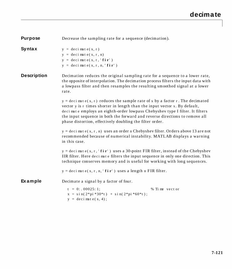
decimate
7-121
7decimatePurpose Decrease the sampling rate for a sequence (decimation).
Syntax y = decimate(x,r)y = decimate(x,r,n)y = decimate(x,r,'fir')y = decimate(x,r,n,'fir')
Description Decimation reduces the original sampling rate for a sequence to a lower rate,the opposite of interpolation. The decimation process filters the input data witha lowpass filter and then resamples the resulting smoothed signal at a lowerrate.
y = decimate(x,r) reduces the sample rate of x by a factor r. The decimatedvector y is r times shorter in length than the input vector x. By default,decimate employs an eighth-order lowpass Chebyshev type I filter. It filtersthe input sequence in both the forward and reverse directions to remove allphase distortion, effectively doubling the filter order.
y = decimate(x,r,n) uses an order nChebyshev filter. Orders above 13 are notrecommended because of numerical instability. MATLAB displays a warningin this case.
y = decimate(x,r,'fir') uses a 30-point FIR filter, instead of the ChebyshevIIR filter. Here decimate filters the input sequence in only one direction. Thistechnique conserves memory and is useful for working with long sequences.
y = decimate(x,r,n,'fir') uses a length n FIR filter.
Example Decimate a signal by a factor of four.
t = 0:.00025:1; % Time vectorx = sin(2*pi*30*t) + sin(2*pi*60*t);y = decimate(x,4);
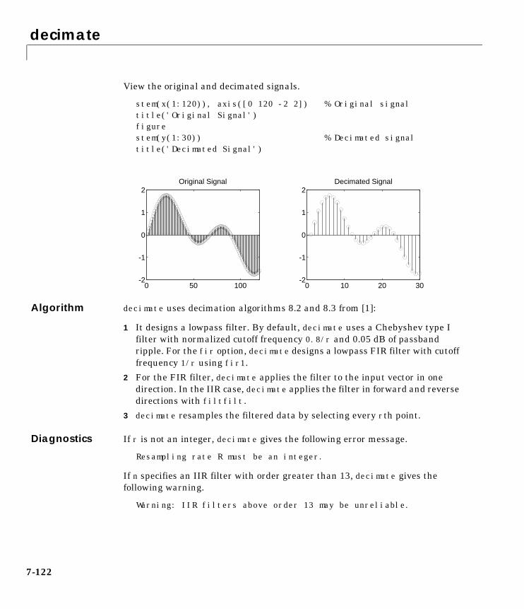
decimate
7-122
View the original and decimated signals.
stem(x(1:120)), axis([0 120 -2 2]) % Original signaltitle('Original Signal')figurestem(y(1:30)) % Decimated signaltitle('Decimated Signal')
Algorithm decimate uses decimation algorithms 8.2 and 8.3 from [1]:
1 It designs a lowpass filter. By default, decimate uses a Chebyshev type Ifilter with normalized cutoff frequency 0.8/r and 0.05 dB of passbandripple. For the fir option, decimate designs a lowpass FIR filter with cutofffrequency 1/r using fir1.
2 For the FIR filter, decimate applies the filter to the input vector in onedirection. In the IIR case, decimate applies the filter in forward and reversedirections with filtfilt.
3 decimate resamples the filtered data by selecting every rth point.
Diagnostics If r is not an integer, decimate gives the following error message.
Resampling rate R must be an integer.
If n specifies an IIR filter with order greater than 13, decimate gives thefollowing warning.
Warning: IIR filters above order 13 may be unreliable.
0 50 100-2
-1
0
1
2Original Signal
0 10 20 30-2
-1
0
1
2Decimated Signal

decimate
7-123
See Also
References [1] IEEE. Programs for Digital Signal Processing. IEEE Press. New York: JohnWiley & Sons, 1979. Chapter 8.
interp Resample data at a higher rate using lowpassinterpolation.
resample Change sampling rate by any rational factor.
spline Cubic spline interpolation (see the MATLABdocumentation).
upfirdn Upsample, apply an FIR filter, and downsample.
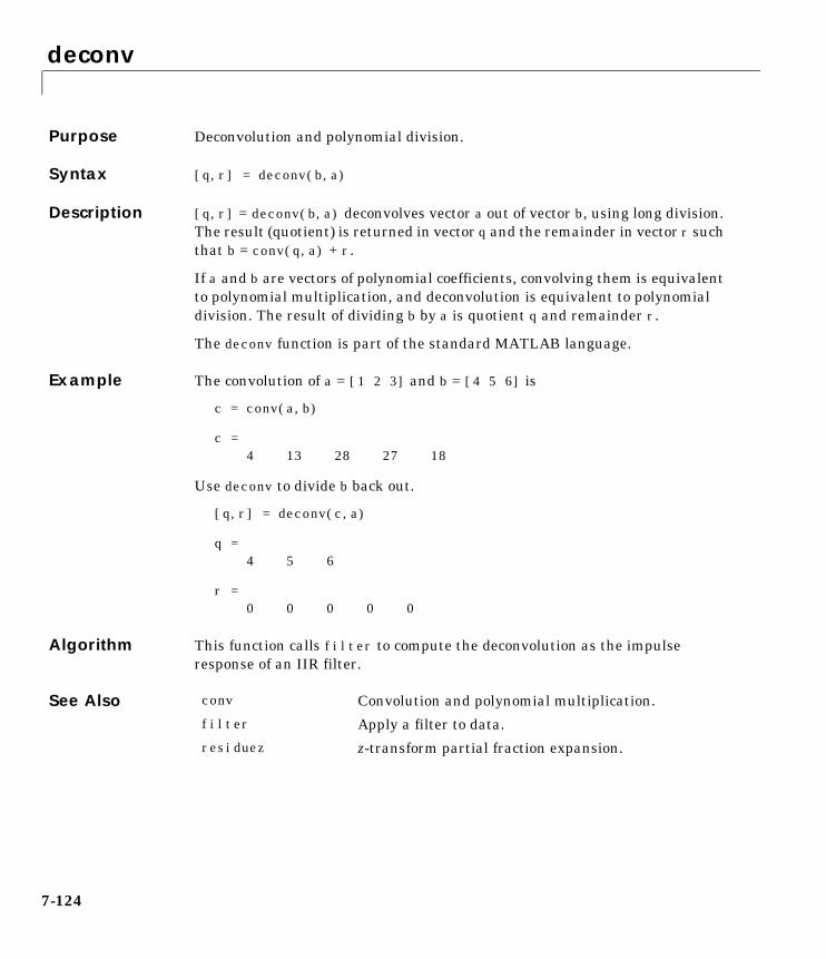
deconv
7-124
7deconvPurpose Deconvolution and polynomial division.
Syntax [q,r] = deconv(b,a)
Description [q,r] = deconv(b,a) deconvolves vector a out of vector b, using long division.The result (quotient) is returned in vector q and the remainder in vector r suchthat b = conv(q,a) + r.
If a and b are vectors of polynomial coefficients, convolving them is equivalentto polynomial multiplication, and deconvolution is equivalent to polynomialdivision. The result of dividing b by a is quotient q and remainder r.
The deconv function is part of the standard MATLAB language.
Example The convolution of a = [1 2 3] and b = [4 5 6] is
c = conv(a,b)
c =4 13 28 27 18
Use deconv to divide b back out.
[q,r] = deconv(c,a)
q =4 5 6
r =0 0 0 0 0
Algorithm This function calls filter to compute the deconvolution as the impulseresponse of an IIR filter.
See Also conv Convolution and polynomial multiplication.
filter Apply a filter to data.
residuez z-transform partial fraction expansion.

demod
7-125
7demodPurpose Demodulation for communications simulation.
Syntax x = demod(y,fc,fs,'method')x = demod(y,fc,fs,'method',opt)x = demod(y,fc,fs,'pwm','centered')[x1,x2] = demod(y,fc,fs,'qam')
Description demod performs demodulation, that is, it obtains the original signal from amodulated version of the signal. demod undoes the operation performed bymodulate.
x = demod(y,fc,fs,'method') and
x = demod(y,fc,fs,'method',opt) demodulate the real carrier signal ywith acarrier frequency fc and sampling frequency fs, using one of the options listedbelow for method. (Note that some methods accept an option, opt.)
amdsb-scoram
Amplitude demodulation, double sideband, suppressedcarrier. Multiplies y by a sinusoid of frequency fc and applies afifth-order Butterworth lowpass filter using filtfilt.
x = y.*cos(2*pi*fc*t);[b,a] = butter(5,fc*2/fs);x = filtfilt(b,a,x);
amdsb-tc Amplitude demodulation, double sideband, transmittedcarrier. Multiplies y by a sinusoid of frequency fc, and applies afifth-order Butterworth lowpass filter using filtfilt.
x = y.*cos(2*pi*fc*t);[b,a] = butter(5,fc*2/fs);x = filtfilt(b,a,x);
If you specify opt, demod subtracts scalar opt from x. The defaultvalue for opt is 0.
amssb Amplitude demodulation, single sideband. Multiplies y by asinusoid of frequency fc and applies a fifth-order Butterworthlowpass filter using filtfilt.
x = y.*cos(2*pi*fc*t);[b,a] = butter(5,fc*2/fs);x = filtfilt(b,a,x);
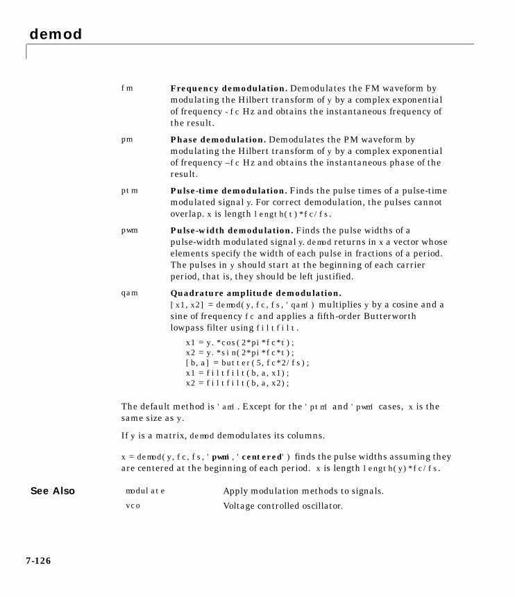
demod
7-126
The default method is 'am'. Except for the 'ptm' and 'pwm' cases, x is thesame size as y.
If y is a matrix, demod demodulates its columns.
x = demod(y,fc,fs,'pwm','centered') finds the pulse widths assuming theyare centered at the beginning of each period. x is length length(y)*fc/fs.
See Also
fm Frequency demodulation. Demodulates the FM waveform bymodulating the Hilbert transform of y by a complex exponentialof frequency -fc Hz and obtains the instantaneous frequency ofthe result.
pm Phase demodulation. Demodulates the PM waveform bymodulating the Hilbert transform of y by a complex exponentialof frequency –fc Hz and obtains the instantaneous phase of theresult.
ptm Pulse-time demodulation. Finds the pulse times of a pulse-timemodulated signal y. For correct demodulation, the pulses cannotoverlap. x is length length(t)*fc/fs.
pwm Pulse-width demodulation. Finds the pulse widths of apulse-width modulated signal y. demod returns in x a vector whoseelements specify the width of each pulse in fractions of a period.The pulses in y should start at the beginning of each carrierperiod, that is, they should be left justified.
qam Quadrature amplitude demodulation.[x1,x2] = demod(y,fc,fs,'qam') multiplies y by a cosine and asine of frequency fc and applies a fifth-order Butterworthlowpass filter using filtfilt.
x1 = y.*cos(2*pi*fc*t);x2 = y.*sin(2*pi*fc*t);[b,a] = butter(5,fc*2/fs);x1 = filtfilt(b,a,x1);x2 = filtfilt(b,a,x2);
modulate Apply modulation methods to signals.
vco Voltage controlled oscillator.
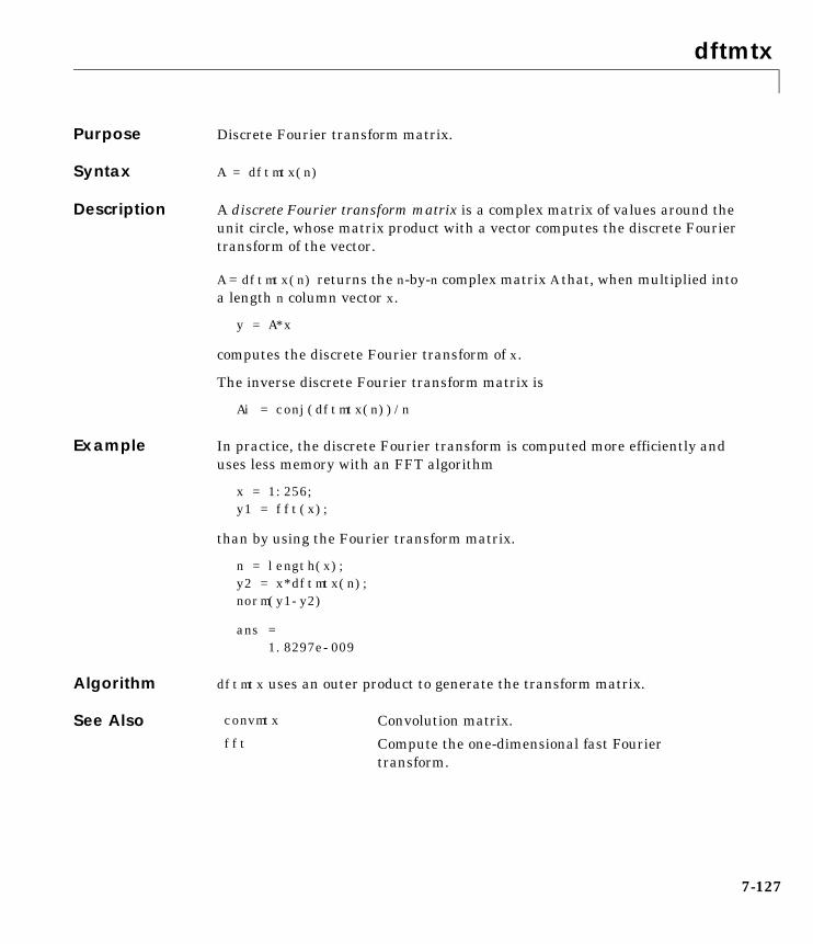
dftmtx
7-127
7dftmtxPurpose Discrete Fourier transform matrix.
Syntax A = dftmtx(n)
Description A discrete Fourier transform matrix is a complex matrix of values around theunit circle, whose matrix product with a vector computes the discrete Fouriertransform of the vector.
A = dftmtx(n) returns the n-by-n complex matrix A that, when multiplied intoa length n column vector x.
y = A*x
computes the discrete Fourier transform of x.
The inverse discrete Fourier transform matrix is
Ai = conj(dftmtx(n))/n
Example In practice, the discrete Fourier transform is computed more efficiently anduses less memory with an FFT algorithm
x = 1:256;y1 = fft(x);
than by using the Fourier transform matrix.
n = length(x);y2 = x*dftmtx(n);norm(y1-y2)
ans =1.8297e-009
Algorithm dftmtx uses an outer product to generate the transform matrix.
See Also convmtx Convolution matrix.
fft Compute the one-dimensional fast Fouriertransform.
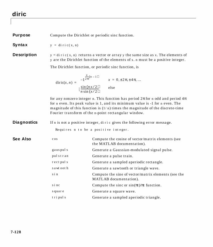
diric
7-128
7diricPurpose Compute the Dirichlet or periodic sinc function.
Syntax y = diric(x,n)
Description y = diric(x,n) returns a vector or array y the same size as x. The elements ofy are the Dirichlet function of the elements of x. n must be a positive integer.
The Dirichlet function, or periodic sinc function, is
for any nonzero integer n. This function has period 2π for n odd and period 4πfor n even. Its peak value is 1, and its minimum value is -1 for n even. Themagnitude of this function is (1/n) times the magnitude of the discrete-timeFourier transform of the n-point rectangular window.
Diagnostics If n is not a positive integer, diric gives the following error message.
Requires n to be a positive integer.
See Also
diric x n,( )1–
x2π------- n 1–( )
x 0 2π± 4π± …, , ,=
nx 2⁄( )sinn x 2⁄( )sin---------------------------- else
=
cos Compute the cosine of vector/matrix elements (seethe MATLAB documentation).
gauspuls Generate a Gaussian-modulated signal pulse.
pulstran Generate a pulse train.
rectpuls Generate a sampled aperiodic rectangle.
sawtooth Generate a sawtooth or triangle wave.
sin Compute the sine of vector/matrix elements (see theMATLAB documentation).
sinc Compute the sinc or sin(πt)/πt function.
square Generate a square wave.
tripuls Generate a sampled aperiodic triangle.
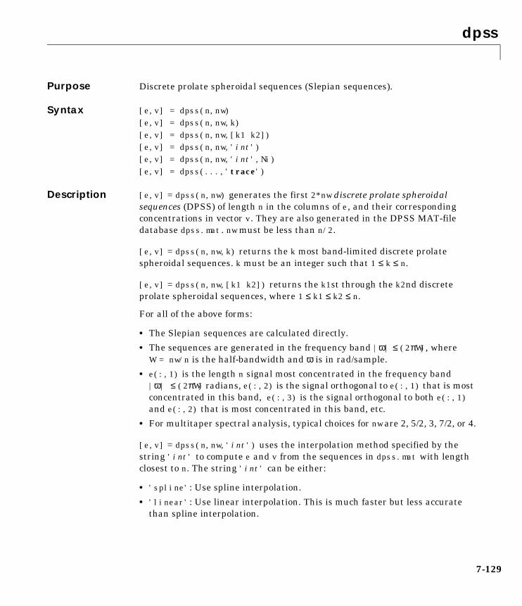
dpss
7-129
7dpssPurpose Discrete prolate spheroidal sequences (Slepian sequences).
Syntax [e,v] = dpss(n,nw)[e,v] = dpss(n,nw,k)[e,v] = dpss(n,nw,[k1 k2])[e,v] = dpss(n,nw,'int')[e,v] = dpss(n,nw,'int',Ni)[e,v] = dpss(...,'trace')
Description [e,v] = dpss(n,nw) generates the first 2*nw discrete prolate spheroidalsequences (DPSS) of length n in the columns of e, and their correspondingconcentrations in vector v. They are also generated in the DPSS MAT-filedatabase dpss.mat. nw must be less than n/2.
[e,v] = dpss(n,nw,k) returns the k most band-limited discrete prolatespheroidal sequences. k must be an integer such that 1 ≤ k ≤ n.
[e,v] = dpss(n,nw,[k1 k2]) returns the k1st through the k2nd discreteprolate spheroidal sequences, where 1 ≤ k1 ≤ k2 ≤ n.
For all of the above forms:
• The Slepian sequences are calculated directly.
• The sequences are generated in the frequency band |ω| ≤ (2πW), where W = nw/n is the half-bandwidth and ω is in rad/sample.
• e(:,1) is the length n signal most concentrated in the frequency band|ω| ≤ (2πW) radians, e(:,2) is the signal orthogonal to e(:,1) that is mostconcentrated in this band, e(:,3) is the signal orthogonal to both e(:,1)and e(:,2) that is most concentrated in this band, etc.
• For multitaper spectral analysis, typical choices for nw are 2, 5/2, 3, 7/2, or 4.
[e,v] = dpss(n,nw,'int') uses the interpolation method specified by thestring 'int' to compute e and v from the sequences in dpss.mat with lengthclosest to n. The string 'int' can be either:
• 'spline': Use spline interpolation.
• 'linear': Use linear interpolation. This is much faster but less accuratethan spline interpolation.
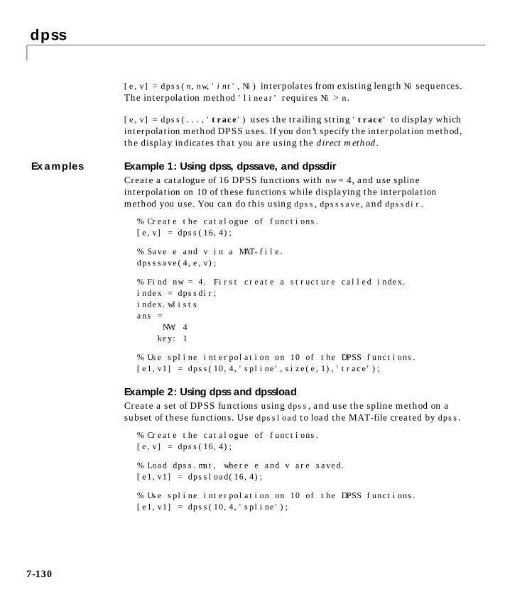
dpss
7-130
[e,v] = dpss(n,nw,'int',Ni) interpolates from existing length Ni sequences.The interpolation method 'linear' requires Ni > n.
[e,v] = dpss(...,'trace') uses the trailing string 'trace' to display whichinterpolation method DPSS uses. If you don’t specify the interpolation method,the display indicates that you are using the direct method.
Examples Example 1: Using dpss, dpssave, and dpssdirCreate a catalogue of 16 DPSS functions with nw = 4, and use splineinterpolation on 10 of these functions while displaying the interpolationmethod you use. You can do this using dpss, dpsssave, and dpssdir.
% Create the catalogue of functions.[e,v] = dpss(16,4);
% Save e and v in a MAT-file. dpsssave(4,e,v);
% Find nw = 4. First create a structure called index.index = dpssdir;index.wlistsans = NW: 4 key: 1
% Use spline interpolation on 10 of the DPSS functions.[e1,v1] = dpss(10,4,'spline',size(e,1),'trace');
Example 2: Using dpss and dpssloadCreate a set of DPSS functions using dpss, and use the spline method on asubset of these functions. Use dpssload to load the MAT-file created by dpss.
% Create the catalogue of functions.[e,v] = dpss(16,4);
% Load dpss.mat, where e and v are saved. [e1,v1] = dpssload(16,4);
% Use spline interpolation on 10 of the DPSS functions.[e1,v1] = dpss(10,4,'spline');
dpss
7-131
See Also
References [1] Percival, D.B., and A.T. Walden. Spectral Analysis for PhysicalApplications: Multitaper and Conventional Univariate Techniques. Cambridge:Cambridge University Press, 1993.
dpssclear Remove discrete prolate spheroidal sequences fromdatabase.
dpssdir Discrete prolate spheroidal sequences databasedirectory.
dpssload Load discrete prolate spheroidal sequences fromdatabase.
dpsssave Save discrete prolate spheroidal sequences indatabase.
pmtm Estimate the power spectral density using themultitaper method (MTM).
dpssclear
7-132
7dpssclearPurpose Remove discrete prolate spheroidal sequences from database.
Syntax dpssclear(n,nw)
Description dpssclear(n,nw) removes sequences with length n and time-bandwidthproduct nw from the DPSS MAT-file database dpss.mat.
See Also dpss Discrete prolate spheroidal sequences (Slepiansequences).
dpssdir Discrete prolate spheroidal sequences databasedirectory.
dpssload Load discrete prolate spheroidal sequences fromdatabase.
dpsssave Save discrete prolate spheroidal sequences indatabase.
dpssdir
7-133
7dpssdirPurpose Discrete prolate spheroidal sequences database directory.
Syntax dpssdirdpssdir(n)dpssdir(nw,'nw')dpssdir(n,nw)index = dpssdir
Description dpssdir manages the database directory that contains the generated DPSSsamples in the DPSS MAT-file database dpss.mat.
dpssdir lists the directory of saved sequences in dpss.mat.
dpssdir(n) lists the sequences saved with length n.
dpssdir(nw,'nw') lists the sequences saved with time-bandwidth product nw.
dpssdir(n,nw) lists the sequences saved with length n and time-bandwidthproduct nw.
index = dpssdir is a structure array describing the DPSS database. Pass n and nw options as for the no output case to get a filtered index.
Examples See “Example 1: Using dpss, dpssave, and dpssdir” on page 7-130.
See Also dpss Discrete prolate spheroidal sequences (Slepiansequences).
dpssclear Remove discrete prolate spheroidal sequences fromdatabase.
dpssload Load discrete prolate spheroidal sequences fromdatabase.
dpsssave Save discrete prolate spheroidal sequences indatabase.

dpssload
7-134
7dpssloadPurpose Load discrete prolate spheroidal sequences from database.
Syntax [e,v] = dpssload(n,nw)
Description [e,v] = dpssload(n,nw) loads all sequences with length n andtime-bandwidth product nw in the columns of e and their correspondingconcentrations in vector v from the DPSS MAT-file database dpss.mat.
Examples See “Example 2: Using dpss and dpssload” on page 7-130.
See Also dpss Discrete prolate spheroidal sequences (Slepiansequences).
dpssclear Remove discrete prolate spheroidal sequences fromdatabase.
dpssdir Discrete prolate spheroidal sequences databasedirectory.
dpsssave Save discrete prolate spheroidal sequences indatabase.
dpsssave
7-135
7dpsssavePurpose Save discrete prolate spheroidal sequences in database.
Syntax dpsssave(nw,e,v)status = dpsssave(nw,e,v)
Description dpsssave(nw,e,v) saves the sequences in the columns of e and theircorresponding concentrations in vector v in the DPSS MAT-file databasedpss.mat.
• It is not necessary to specify sequence length, because the length of thesequence is determined by the number of rows of e.
• nw is the time-bandwidth product that was specified when the sequence wascreated using dpss.
status = dpsssave(nw,e,v) returns 0 if the save was successful and 1 if therewas an error.
Examples See “Example 1: Using dpss, dpssave, and dpssdir” on page 7-130.
See Also dpss Discrete prolate spheroidal sequences (Slepiansequences).
dpssclear Remove discrete prolate spheroidal sequences fromdatabase.
dpssdir Discrete prolate spheroidal sequences databasedirectory.
dpssload Load discrete prolate spheroidal sequences fromdatabase.

ellip
7-136
7ellipPurpose Elliptic (Cauer) filter design.
Syntax [b,a] = ellip(n,Rp,Rs,Wn)[b,a] = ellip(n,Rp,Rs,Wn,'ftype')[b,a] = ellip(n,Rp,Rs,Wn,'s')[b,a] = ellip(n,Rp,Rs,Wn,'ftype','s')[z,p,k] = ellip(...)[A,B,C,D] = ellip(...)
Description ellip designs lowpass, bandpass, highpass, and bandstop digital and analogelliptic filters. Elliptic filters offer steeper rolloff characteristics thanButterworth or Chebyshev filters, but are equiripple in both the pass- andstopbands. In general, elliptic filters meet given performance specificationswith the lowest order of any filter type.
Digital Domain
[b,a] = ellip(n,Rp,Rs,Wn) designs an order n lowpass digital elliptic filterwith cutoff frequency Wn, Rp dB of ripple in the passband, and a stopband Rs dBdown from the peak value in the passband. It returns the filter coefficients in thelength n+1 row vectors b and a, with coefficients in descending powers of z.
The cutoff frequency is the edge of the passband, at which the magnituderesponse of the filter is -Rp dB. For ellip, the cutoff frequency Wn is a numberbetween 0 and 1, where 1 corresponds to half the sampling frequency (Nyquistfrequency). Smaller values of passband ripple Rp and larger values of stopbandattenuation Rs both lead to wider transition widths (shallower rolloffcharacteristics).
If Wn is a two-element vector, Wn = [w1 w2], ellip returns an order 2*nbandpass filter with passband w1 < ω < w2.
H z( )B z( )A z( )----------- b 1( ) b 2( )z 1– b n 1+( )z n–+ + +
1 a 2( )z 1– a n 1+( )z n–+ + +------------------------------------------------------------------------------------= =
ellip
7-137
[b,a] = ellip(n,Rp,Rs,Wn,'ftype') designs a highpass or bandstop filter,where the string 'ftype' is either:
• 'high' for a highpass digital filter with cutoff frequency Wn
• 'stop' for an order 2*n bandstop digital filter if Wn is a two-element vector,Wn = [w1 w2]. The stopband is w1 < ω < w2.
With different numbers of output arguments, ellip directly obtains otherrealizations of the filter. To obtain zero-pole-gain form, use three outputarguments as shown below.
[z,p,k] = ellip(n,Rp,Rs,Wn) or
[z,p,k] = ellip(n,Rp,Rs,Wn,'ftype') returns the zeros and poles in lengthn column vectors z and p and the gain in the scalar k.
To obtain state-space form, use four output arguments as shown below.
[A,B,C,D] = ellip(n,Rp,Rs,Wn) or
[A,B,C,D] = ellip(n,Rp,Rs,Wn,'ftype') where A, B, C, and D are
and u is the input, x is the state vector, and y is the output.
Analog Domain
[b,a] = ellip(n,Rp,Rs,Wn,'s') designs an order n lowpass analog ellipticfilter with cutoff frequency Wn and returns the filter coefficients in the lengthn+1 row vectors b and a, in descending powers of s, derived from the transferfunction
The cutoff frequency is the edge of the passband, at which the magnituderesponse of the filter is -Rp dB. For ellip, the cutoff frequency Wn must begreater than 0.
x n 1+[ ] Ax n[ ] Bu n[ ]+=
y n[ ] Cx n[ ] Du n[ ]+=
H s( )B s( )A s( )----------- b 1( )sn b 2( )sn 1– b n 1+( )+ + +
sn a 2( )sn 1– a n 1+( )+ + +-------------------------------------------------------------------------------------= =
ellip
7-138
If Wn is a two-element vector with w1 < w2, then ellip(n,Rp,Rs,Wn,'s')returns an order 2*n bandpass analog filter with passband w1 < ω < w2.
[b,a] = ellip(n,Rp,Rs,Wn,'ftype','s') designs a highpass or bandstopfilter.
With different numbers of output arguments, ellip directly obtains otherrealizations of the analog filter. To obtain zero-pole-gain form, use three outputarguments as shown below.
[z,p,k] = ellip(n,Rp,Rs,Wn,'s') or
[z,p,k] = ellip(n,Rp,Rs,Wn,'ftype','s') returns the zeros and poles inlength n or 2*n column vectors z and p and the gain in the scalar k.
To obtain state-space form, use four output arguments as shown below.
[A,B,C,D] = ellip(n,Rp,Rs,Wn,'s') or
[A,B,C,D] = ellip(n,Rp,Rs,Wn,'ftype','s') where A, B, C, and D are
and u is the input, x is the state vector, and y is the output.
Examples Example 1For data sampled at 1000 Hz, design a sixth-order lowpass elliptic filter with acutoff frequency of 300 Hz, 3 dB of ripple in the passband, and 50 dB ofattenuation in the stopband.
[b,a] = ellip(6,3,50,300/500);
The filter’s frequency response is
freqz(b,a,512,1000)title('n=6 Lowpass Elliptic Filter')
x· Ax Bu+=
y Cx Du+=

ellip
7-139
Example 2Design a 20th-order bandpass elliptic filter with a passband from 100 to 200 Hzand plot its impulse response.
n = 10; Rp = 0.5; Rs = 20;Wn = [100 200]/500;[b,a] = ellip(n,Rp,Rs,Wn);[y,t] = impz(b,a,101); stem(t,y)title('Impulse Response of n=10 Elliptic Filter')
0 50 100 150 200 250 300 350 400 450 500−500
−400
−300
−200
−100
0
100
Frequency (Hz)
Ph
ase
(d
eg
ree
s)0 50 100 150 200 250 300 350 400 450 500
−100
−80
−60
−40
−20
0
Frequency (Hz)M
ag
nitu
de
(d
B)
n=6 Lowpass Elliptic Filter

ellip
7-140
Limitations For high order filters, the state-space form is the most numerically accurate,followed by the zero-pole-gain form. The transfer function form is the leastaccurate; numerical problems can arise for filter orders as low as 15.
Algorithm The design of elliptic filters is the most difficult and computationally intensiveof the Butterworth, Chebyshev type I and II, and elliptic designs. ellip uses afive-step algorithm:
1 It finds the lowpass analog prototype poles, zeros, and gain using theellipap function.
2 It converts the poles, zeros, and gain into state-space form.
3 It transforms the lowpass filter to a bandpass, highpass, or bandstop filterwith the desired cutoff frequencies using a state-space transformation.
4 For digital filter design, ellip uses bilinear to convert the analog filterinto a digital filter through a bilinear transformation with frequencyprewarping. Careful frequency adjustment guarantees that the analogfilters and the digital filters will have the same frequency responsemagnitude at Wn or w1 and w2.
5 It converts the state-space filter back to transfer function or zero-pole-gainform, as required.
0 10 20 30 40 50 60 70 80 90 100-0.2
-0.15
-0.1
-0.05
0
0.05
0.1
0.15
0.2Impulse Response of n = 10 Elliptic Filter

ellip
7-141
See Also besself Design a Bessel analog filter.
butter Design a Butterworth analog or digital filter.
cheby1 Design a Chebyshev type I filter (passband ripple).
cheby2 Design a Chebyshev type II filter (stopband ripple).
ellipap Design an elliptic analog lowpass filter prototype.
ellipord Calculate the order for an elliptic filter.
ellipap
7-142
7ellipapPurpose Elliptic analog lowpass filter prototype.
Syntax [z,p,k] = ellipap(n,Rp,Rs)
Description [z,p,k] = ellipap(n,Rp,Rs) returns the zeros, poles, and gain of an order nelliptic analog lowpass filter prototype, with Rp dB of ripple in the passband,and a stopband Rs dB down from the peak value in the passband. The zeros andpoles are returned in length n column vectors z and p and the gain in scalar k.If n is odd, z is length n - 1. The transfer function is
Elliptic filters offer steeper rolloff characteristics than Butterworth andChebyshev filters, but they are equiripple in both the passband and thestopband. Of the four classical filter types, elliptic filters usually meet a givenset of filter performance specifications with the lowest filter order.
ellip sets the cutoff frequency of the elliptic filter to 1 for a normalizedresult. The cutoff frequency is the frequency at which the passband ends andthe filter has a magnitude response of 10-Rp/20.
Algorithm ellipap uses the algorithm outlined in [1]. It employs the M-file ellipk tocalculate the complete elliptic integral of the first kind and the M-file ellipjto calculate Jacobi elliptic functions.
See Also
References [1] Parks, T.W., and C.S. Burrus. Digital Filter Design. New York: John Wiley& Sons, 1987. Chapter 7.
H s( )z s( )p s( )---------- k s z 1( )–( ) s z 2( )–( ) s z n( )–( )
s p 1( )–( ) s p 2( )–( ) s p n( )–( )--------------------------------------------------------------------------------= =
ω0
besselap Bessel analog lowpass filter prototype.
buttap Butterworth analog lowpass filter prototype.
cheb1ap Chebyshev type I analog lowpass filter prototype.
cheb2ap Chebyshev type II analog lowpass filter prototype.
ellip Elliptic (Cauer) filter design.
ellipord
7-143
7ellipordPurpose Calculate the minimum order for elliptic filters.
Syntax [n,Wn] = ellipord(Wp,Ws,Rp,Rs)[n,Wn] = ellipord(Wp,Ws,Rp,Rs,'s')
Description ellipord calculates the minimum order of a digital or analog elliptic filterrequired to meet a set of filter design specifications.
Digital Domain
[n,Wn] = ellipord(Wp,Ws,Rp,Rs) returns the lowest order n of the ellipticfilter that loses no more than Rp dB in the passband and has at least Rs dB ofattenuation in the stopband. The scalar (or vector) of corresponding cutofffrequencies Wn, is also returned. Use the output arguments n and Wn in ellip.
Choose the input arguments to specify the stopband and passband according tothe following table.
Table 7-7: Description of Stopband and Passband Filter Parameters
Wp Passband corner frequency Wp, the cutoff frequency, is a scalaror a two-element vector with values between 0 and 1, with 1corresponding to the normalized Nyquist frequency, π radiansper sample.
Ws Stopband corner frequency Ws, is a scalar or a two-elementvector with values between 0 and 1, with 1 corresponding tothe normalized Nyquist frequency.
Rp Passband ripple, in decibels. Twice this value specifies themaximum permissible passband width in decibels.
Rs Stopband attenuation, in decibels. This value is the number ofdecibels the stopband is attenuated with respect to thepassband response.
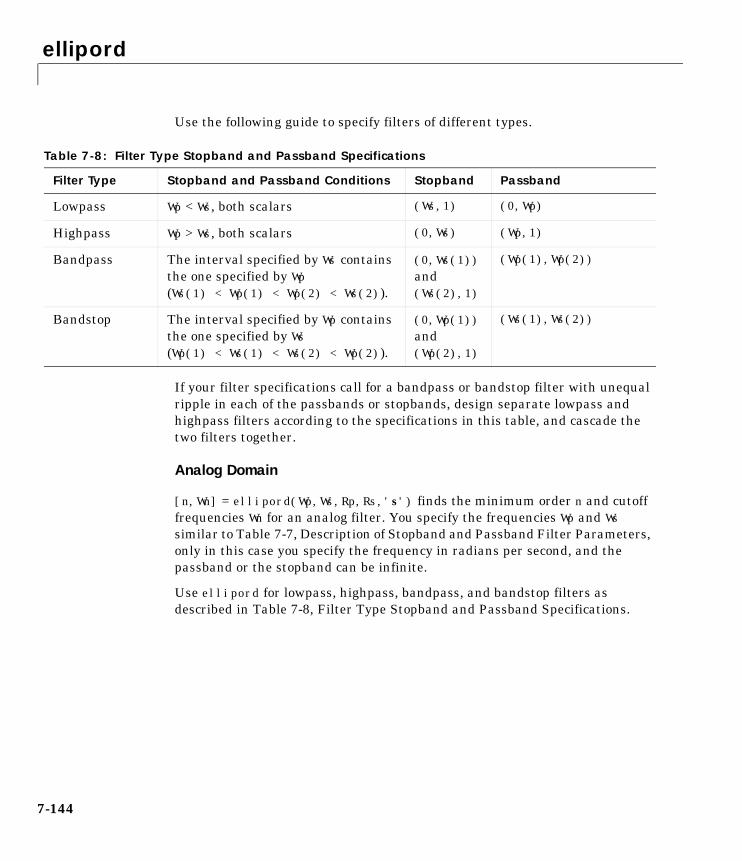
ellipord
7-144
Use the following guide to specify filters of different types.
If your filter specifications call for a bandpass or bandstop filter with unequalripple in each of the passbands or stopbands, design separate lowpass andhighpass filters according to the specifications in this table, and cascade thetwo filters together.
Analog Domain
[n,Wn] = ellipord(Wp,Ws,Rp,Rs,'s') finds the minimum order n and cutofffrequencies Wn for an analog filter. You specify the frequencies Wp and Wssimilar to Table 7-7, Description of Stopband and Passband Filter Parameters,only in this case you specify the frequency in radians per second, and thepassband or the stopband can be infinite.
Use ellipord for lowpass, highpass, bandpass, and bandstop filters asdescribed in Table 7-8, Filter Type Stopband and Passband Specifications.
Table 7-8: Filter Type Stopband and Passband Specifications
Filter Type Stopband and Passband Conditions Stopband Passband
Lowpass Wp < Ws, both scalars (Ws,1) (0,Wp)
Highpass Wp > Ws, both scalars (0,Ws) (Wp,1)
Bandpass The interval specified by Ws containsthe one specified by Wp(Ws(1) < Wp(1) < Wp(2) < Ws(2)).
(0,Ws(1))and(Ws(2),1)
(Wp(1),Wp(2))
Bandstop The interval specified by Wp containsthe one specified by Ws(Wp(1) < Ws(1) < Ws(2) < Wp(2)).
(0,Wp(1))and(Wp(2),1)
(Ws(1),Ws(2))
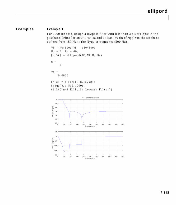
ellipord
7-145
Examples Example 1For 1000 Hz data, design a lowpass filter with less than 3 dB of ripple in thepassband defined from 0 to 40 Hz and at least 60 dB of ripple in the stopbanddefined from 150 Hz to the Nyquist frequency (500 Hz).
Wp = 40/500; Ws = 150/500;Rp = 3; Rs = 60;[n,Wn] = ellipord(Wp,Ws,Rp,Rs)
n = 4
Wn = 0.0800
[b,a] = ellip(n,Rp,Rs,Wn);freqz(b,a,512,1000);title('n=4 Elliptic Lowpass Filter')
0 50 100 150 200 250 300 350 400 450 500−400
−300
−200
−100
0
100
Frequency (Hz)
Ph
ase
(d
eg
ree
s)
0 50 100 150 200 250 300 350 400 450 500−120
−100
−80
−60
−40
−20
0
Frequency (Hz)
Ma
gn
itud
e (
dB
)
n=4 Elliptic Lowpass Filter

ellipord
7-146
Example 2Now design a bandpass filter with a passband from 60 Hz to 200 Hz, with lessthan 3 dB of ripple in the passband, and 40 dB attenuation in the stopbandsthat are 50 Hz wide on both sides of the passband.
Wp = [60 200]/500; Ws = [50 250]/500;Rp = 3; Rs = 40;[n,Wn] = ellipord(Wp,Ws,Rp,Rs)
n = 5Wn = 0.1200 0.4000
[b,a] = ellip(n,Rp,Rs,Wn);freqz(b,a,512,1000);title('n=5 Elliptic Bandpass Filter')
0 50 100 150 200 250 300 350 400 450 500−500
0
500
Frequency (Hz)
Ph
ase
(d
eg
ree
s)
0 50 100 150 200 250 300 350 400 450 500−300
−250
−200
−150
−100
−50
0
Frequency (Hz)
Ma
gn
itud
e (
dB
)
n=5 Elliptic Bandpass Filter
ellipord
7-147
Algorithm ellipord uses the elliptic lowpass filter order prediction formula describedin [1]. The function performs its calculations in the analog domain for both theanalog and digital cases. For the digital case, it converts the frequencyparameters to the s-domain before estimating the order and naturalfrequencies, and then converts them back to the z-domain.
ellipord initially develops a lowpass filter prototype by transforming thepassband frequencies of the desired filter to 1 rad/s (for low- and highpassfilters) and to -1 and 1 rad/s (for bandpass and bandstop filters). It thencomputes the minimum order required for a lowpass filter to meet the stopbandspecification.
See Also
References [1] Rabiner, L.R., and B. Gold. Theory and Application of Digital SignalProcessing. Englewood Cliffs, NJ: Prentice-Hall, 1975. Pg. 241.
buttord Calculate the order for a Butterworth filter.
cheb1ord Calculate the order for a Chebyshev type I filter.
cheb2ord Calculate the order for a Chebyshev type II filter.
ellip Design an elliptic (Cauer) filter.

eqtflength
7-148
7eqtflengthPurpose Make the lengths of a transfer function’s numerator and denominator equal.
Syntax [b,a] = eqtflength(num,den)
Description [b,a] = eqtflength(num,den) modifies the vector num and/or the vector den,so that the resulting output vectors b and a have the same length. The inputvectors num and den may have different lengths. The vector num represents thenumerator polynomial of a given discrete-time transfer function, and the vectorden represents its numerator. The resulting numerator b and denominator arepresent the same discrete-time transfer function, but these vectors have thesame length.
Use eqtflength to obtain a numerator and denominator of equal length beforeapplying transfer function conversion functions such as tf2ss and tf2zp todiscrete-time models.
Examples num = [1 0.5];den = [1 0.75 0.6 0];[b,a] = eqtflength(num,den)
b = 1.0000 0.5000 0a = 1.0000 0.7500 0.6000
Algorithm eqtflength(num,den) appends zeros to either num or den as necessary. If bothnum and den have trailing zeros in common, these are removed.
See Also tf2ss Convert a transfer function to state-space form.
tf2zp Convert a transfer function to zero-pole-gain form.
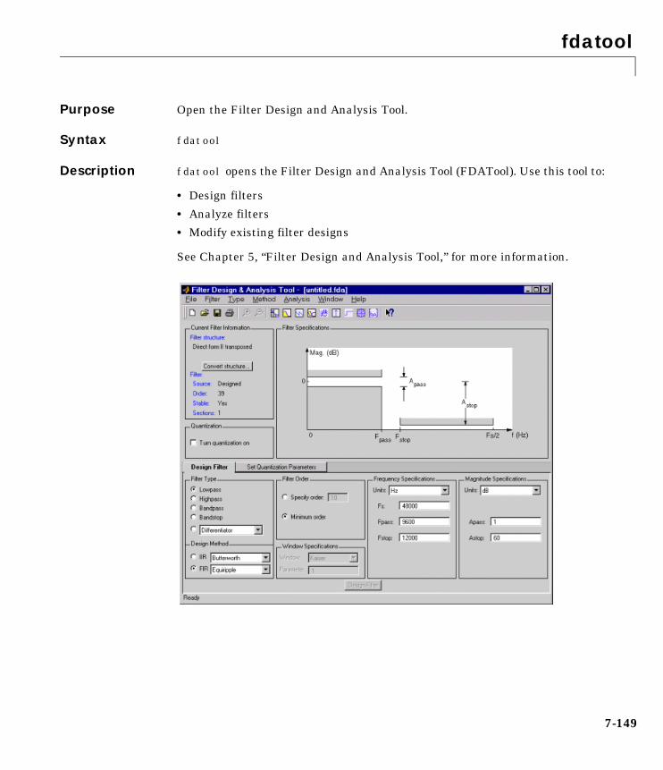
fdatool
7-149
7fdatoolPurpose Open the Filter Design and Analysis Tool.
Syntax fdatool
Description fdatool opens the Filter Design and Analysis Tool (FDATool). Use this tool to:
• Design filters
• Analyze filters
• Modify existing filter designs
See Chapter 5, “Filter Design and Analysis Tool,” for more information.

fdatool
7-150
Remarks The Filter Design and Analysis Tool provides more design methods than theSPTool Filter Designer.
See Also sptool Open the signal processing GUI.

fft
7-151
7fftPurpose Compute the one-dimensional fast Fourier transform.
Syntax y = fft(x)y = fft(x,n)
Description fft computes the discrete Fourier transform of a vector or matrix. Thisfunction implements the transform given by
where WN = e-j(2π/N) and N = length(x). Note that the series is indexed asn + 1 and k + 1 instead of the usual n and k because MATLAB vectors run from1 to N instead of from 0 to N-1.
y = fft(x) is the discrete Fourier transform of vector x, computed with a fastFourier transform (FFT) algorithm. If x is a matrix, y is the FFT of each columnof the matrix.
y = fft(x,n) is the n-point FFT. If the length of x is less than n, fft pads xwith trailing zeros to length n. If the length of x is greater than n, fft truncatesthe sequence x. If x is an array, fft adjusts the length of the columns in thesame manner.
The fft function is part of the standard MATLAB language.
Examples A common use of the Fourier transform is to find the frequency components ofa time-domain signal buried in noise. Consider data sampled at 1000 Hz. Forma signal consisting of 50 Hz and 120 Hz sinusoids and corrupt the signal withzero-mean random noise.
randn('state',0)t = 0:0.001:0.6;x = sin(2*pi*50*t) + sin(2*pi*120*t);y = x + 2*randn(1,length(t));plot(y(1:50))
X k 1+( ) x n 1+( )Wnkn
n 0=
N 1–
=
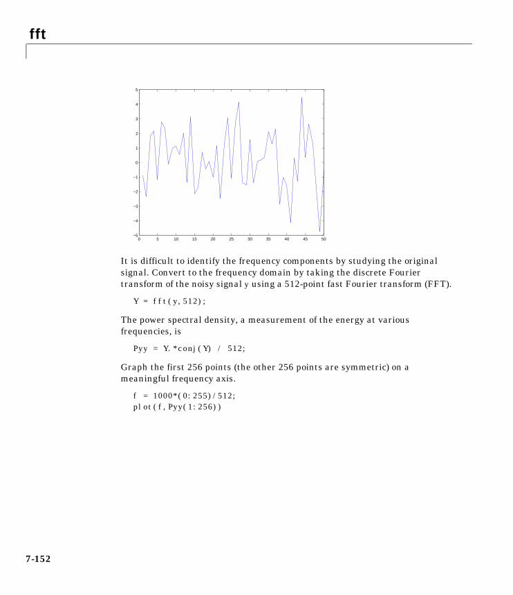
fft
7-152
It is difficult to identify the frequency components by studying the originalsignal. Convert to the frequency domain by taking the discrete Fouriertransform of the noisy signal y using a 512-point fast Fourier transform (FFT).
Y = fft(y,512);
The power spectral density, a measurement of the energy at variousfrequencies, is
Pyy = Y.*conj(Y) / 512;
Graph the first 256 points (the other 256 points are symmetric) on ameaningful frequency axis.
f = 1000*(0:255)/512;plot(f,Pyy(1:256))
0 5 10 15 20 25 30 35 40 45 50−5
−4
−3
−2
−1
0
1
2
3
4
5
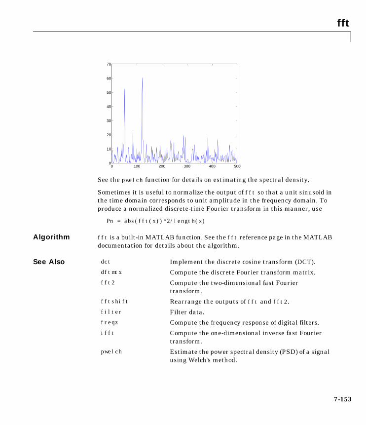
fft
7-153
See the pwelch function for details on estimating the spectral density.
Sometimes it is useful to normalize the output of fft so that a unit sinusoid inthe time domain corresponds to unit amplitude in the frequency domain. Toproduce a normalized discrete-time Fourier transform in this manner, use
Pn = abs(fft(x))*2/length(x)
Algorithm fft is a built-in MATLAB function. See the fft reference page in the MATLABdocumentation for details about the algorithm.
See Also
0 100 200 300 400 5000
10
20
30
40
50
60
70
dct Implement the discrete cosine transform (DCT).
dftmtx Compute the discrete Fourier transform matrix.
fft2 Compute the two-dimensional fast Fouriertransform.
fftshift Rearrange the outputs of fft and fft2.
filter Filter data.
freqz Compute the frequency response of digital filters.
ifft Compute the one-dimensional inverse fast Fouriertransform.
pwelch Estimate the power spectral density (PSD) of a signalusing Welch’s method.
fft2
7-154
7fft2Purpose Compute the two-dimensional fast Fourier transform.
Syntax Y = fft2(X)Y = fft2(X,m,n)
Description Y = fft2(X) performs a two-dimensional FFT, producing a result Y with thesame size as X. If X is a vector, Y has the same orientation as X.
Y = fft2(X,m,n) truncates or zero pads X, if necessary, to create an m-by-narray before performing the FFT. The result Y is also m-by-n.
The fft2 function is part of the standard MATLAB language.
Algorithm fft2(x) is simply
fft(fft(x).').'
This computes the one-dimensional fft of each column of x, then of each rowof the result. The time required to compute fft2(x) depends on the number ofprime factors in [m,n] = size(x). fft2 is fastest when m and n are powers of 2.
See Also fft One-dimensional fast Fourier transform.
fftshift Rearrange the outputs of fft and fft2.
ifft One-dimensional inverse fast Fourier transform.
ifft2 Two-dimensional inverse fast Fourier transform.
fftfilt
7-155
7fftfiltPurpose FFT-based FIR filtering using the overlap-add method.
Syntax y = fftfilt(b,x)y = fftfilt(b,x,n)
Description fftfilt filters data using the efficient FFT-based method of overlap-add, afrequency domain filtering technique that works only for FIR filters.
y = fftfilt(b,x) filters the data in vector x with the filter described bycoefficient vector b. It returns the data vector y. The operation performed byfftfilt is described in the time domain by the difference equation
An equivalent representation is the z-transform or frequency domain description
By default, fftfilt chooses an FFT length and data block length thatguarantee efficient execution time.
y = fftfilt(b,x,n) uses an FFT length of nfft = 2^nextpow2(n) and a datablock length of nfft - length(b) + 1.
fftfilt works for both real and complex inputs.
Examples Show that the results from fftfilt and filter are identical.
b = [1 2 3 4];x = [1 zeros(1,99)]';norm(fftfilt(b,x) - filter(b,1,x))
ans =9.5914e-15
Algorithm fftfilt uses fft to implement the overlap-add method [1], a technique thatcombines successive frequency domain filtered blocks of an input sequence.fftfilt breaks an input sequence x into length L data blocks
y n( ) b 1( )x n( ) b 2( )x n 1–( ) b nb 1+( )x n nb–( )+ + +=
Y z( ) b 1( ) b 2( )z 1– b nb 1+( )z nb–+ + +( )X z( )=
xL 2L 3L ceil(nx/L)*L
. . .
fftfilt
7-156
and convolves each block with the filter b by
y = ifft(fft(x(i:i+L-1),nfft).*fft(b,nfft));
where nfft is the FFT length. fftfilt overlaps successive output sections bynb-1 points, where nb is the length of the filter, and sums them.
fftfilt chooses the key parameters L and nfft in different ways, dependingon whether you supply an FFT length n and on the lengths of the filter andsignal. If you do not specify a value for n (which determines FFT length),fftfilt chooses these key parameters automatically:
• If length(x)is greater than length(b), fftfilt chooses values thatminimize the number of blocks times the number of flops per FFT.
• If length(b) is greater than or equal to length(x), fftfilt uses a singleFFT of length
2^nextpow2(length(b) + length(x) - 1)
This essentially computesy = ifft(fft(B,nfft).*fft(X,nfft))
If you supply a value for n, fftfilt chooses an FFT length, nfft, of2^nextpow2(n)and a data block length of nfft - length(b) + 1. If n is less thanlength(b), fftfilt sets n to length(b).
See Also
References [1] Oppenheim, A.V., and R.W. Schafer, Discrete-Time Signal Processing,Prentice-Hall, 1989.
nb–1L
nb–12L
nb–13L. . .
conv Convolution and polynomial multiplication.
filter Filter data with a recursive (IIR) or nonrecursive(FIR) filter.
filtfilt Zero-phase digital filtering.

fftshift
7-157
7fftshiftPurpose Rearrange the outputs of the FFT functions.
Syntax y = fftshift(x)
Description y = fftshift(x) rearranges the outputs of fft and fft2 by moving the zerofrequency component to the center of the spectral density, which is sometimesa more convenient form.
For vectors, fftshift(x) returns a vector with the left and right halvesswapped.
For arrays, fftshift(x) swaps quadrants one and three with quadrants twoand four.
The fftshift function is part of the standard MATLAB language.
Examples For any array X
Y = fft2(x)
has Y(1,1) = sum(sum(X)); the DC component of the signal is in the upper-leftcorner of the two-dimensional FFT. For
Z = fftshift(Y)
the DC component is near the center of the matrix.
See Also fft One-dimensional fast Fourier transform.
fft2 Two-dimensional fast Fourier transform.
filter
7-158
7filterPurpose Filter data with a recursive (IIR) or nonrecursive (FIR) filter.
Syntax y = filter(b,a,x)[y,zf] = filter(b,a,x)[...] = filter(b,a,x,zi)[...] = filter(b,a,x,zi,dim)
Description y = filter(b,a,x) filters the data in vector x with the filter described bycoefficient vectors a and b to create the filtered data vector y. When x is amatrix, filter operates on the columns of x. When x is an N-dimensional array,filter operates on the first nonsingleton dimension. a(1) cannot be 0, and ifa(1) ≠ 1, filter normalizes the filter coefficients by a(1).
[y,zf] = filter(b,a,x) returns the final values zf of the state vector. Whenx is a vector, the size of the final condition vector zf ismax(length(b),length(a))-1, the number of delays in the filter. When x is amultidimensional array, zf is an s-by-c matrix, where:
• s is the number of delays in the filter.
• c is prod(size(x))/size(x,dim), where dim is the dimension into which youare filtering (the first nonsingleton dimension by default).
[...] = filter(b,a,x,zi) specifies initial state conditions in the vector zi.The size of the initial condition vector zi must be the same asmax(length(b),length(a))-1, the number of delays in the filter.
[...] = filter(b,a,x,zi,dim) filters the input data located along thedimension dim of x. Set zi to the empty vector [] to use zero initial conditions.
The filter function is part of the standard MATLAB language.
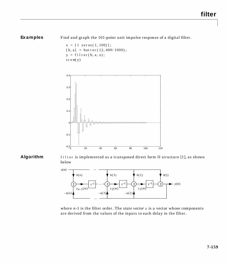
filter
7-159
Examples Find and graph the 101-point unit impulse response of a digital filter.
x = [1 zeros(1,100)];[b,a] = butter(12,400/1000);y = filter(b,a,x);stem(y)
Algorithm filter is implemented as a transposed direct form II structure [1], as shownbelow
where n-1 is the filter order. The state vector z is a vector whose componentsare derived from the values of the inputs to each delay in the filter.
0 20 40 60 80 100 120-0.2
-0.1
0
0.1
0.2
0.3
0.4
Σ Σ Σz -1 z -1
x(m)
y(m)
b(3) b(2) b(1)
–a(3) –a(2)
z1(m)z2(m)Σ z -1
b(n)
–a(n)
zn -1(m)
...
...
...

filter
7-160
The operation of filter at sample m is implemented using the transposeddirect form II structure. This is calculated by the time domain differenceequations for y and the states zi.
Note the division by a(1). For efficient computation, select this coefficient to bea power of 2.
You can use filtic to generate the state vector zi(0) from past inputs andoutputs.
The input-output description of this filtering operation in the z-transformdomain is a rational transfer function.
See Also
References [1] Oppenheim, A.V., and R.W. Schafer, Discrete-Time Signal Processing,Prentice-Hall, 1989, pp. 311-312.
y m( )b 1( )x m( ) z1 m 1–( )+( )
a 1( )----------------------------------------------------------=
z1 m( ) b 2( )x m( ) z2 m 1–( ) a 2( )y m( )–+=
=
zn 2– m( ) b n 1–( )x m( ) zn 1– m 1–( ) a n 1–( )y m( )–+=
zn 1– m( ) b n( )x m( ) a n( )y m( )–=
Y z( )b 1( ) b 2( )z 1– b nb 1+( )z nb–+ + +a 1( ) a 2( )z 1– a na 1+( )z na–+ + +--------------------------------------------------------------------------------------------X z( )=
fftfilt FFT-based FIR filtering using the overlap-addmethod.
filter2 Two-dimensional digital filtering.
filtfilt Zero-phase digital filtering.
filtic Make initial conditions for filter function.
filter2
7-161
7filter2Purpose Two-dimensional digital filtering.
Syntax Y = filter2(B,X)Y = filter2(B,X,'shape')
Description Y = filter2(B,X) filters the two-dimensional data in X with thetwo-dimensional FIR filter in the matrix B. The result, Y, is computed usingtwo-dimensional convolution and is the same size as X.
Y = filter2(B,X,'shape') returns Y computed with size specified by'shape':
• 'same' returns the central part of the convolution that is the same size as X(default).
• 'full' returns the full two-dimensional convolution, when size(Y) exceedssize(X).
• 'valid' returns only those parts of the convolution that are computedwithout the zero-padded edges, when size(Y) is less than size(X).
The filter2 function is part of the standard MATLAB language.
Algorithm The filter2 function uses conv2 to compute the full two-dimensionalconvolution of the FIR filter with the input matrix. By default, filter2extracts and returns the central part of the convolution that is the same size asthe input matrix. Use the 'shape' parameter to specify an alternate part of theconvolution for return.
See Also conv2 Two-dimensional convolution.
filter Filter data with a recursive (IIR) or nonrecursive(FIR) filter.
filtfilt
7-162
7filtfiltPurpose Zero-phase digital filtering.
Syntax y = filtfilt(b,a,x)
Description y = filtfilt(b,a,x) performs zero-phase digital filtering by processing theinput data in both the forward and reverse directions (see problem 5.39 in [1]).After filtering in the forward direction, it reverses the filtered sequence andruns it back through the filter. The resulting sequence has precisely zero-phasedistortion and double the filter order. filtfilt minimizes start-up and endingtransients by matching initial conditions, and works for both real and complexinputs.
Note that filtfilt should not be used with differentiator and Hilbert FIRfilters, since the operation of these filters depends heavily on their phaseresponse.
Algorithm filtfilt is an M-file that uses the filter function. In addition to theforward-reverse filtering, it attempts to minimize startup transients byadjusting initial conditions to match the DC component of the signal and byprepending several filter lengths of a flipped, reflected copy of the input signal.
See Also
References [1] Oppenheim, A.V., and R.W. Schafer, Discrete-Time Signal Processing,Prentice-Hall, 1989, pp. 311-312.
fftfilt FFT-based FIR filtering using the overlap-addmethod.
filter Filter data with a recursive (IIR) or nonrecursive(FIR) filter.
filter2 Two-dimensional digital filtering.

filtic
7-163
7filticPurpose Find initial conditions for a transposed direct form II filter implementation.
Syntax z = filtic(b,a,y,x)z = filtic(b,a,y)
Description z = filtic(b,a,y,x) finds the initial conditions, z, for the delays in thetransposed direct form II filter implementation given past outputs y andinputs x. The vectors b and a represent the numerator and denominatorcoefficients, respectively, of the filter’s transfer function.
The vectors x and y contain the most recent input or output first, and oldestinput or output last.
where nb is length(b)-1 (the numerator order) and na is length(a)-1 (thedenominator order). If length(x) is less than nb, filtic pads it with zeros tolength nb; if length(y) is less than na, filtic pads it with zeros to length na.Elements of x beyond x(nb-1) and elements of y beyond y(na-1) areunnecessary so filtic ignores them.
Output z is a column vector of length equal to the larger of nb and na.z describes the state of the delays given past inputs x and past outputs y.
z = filtic(b,a,y) assumes that the input x is 0 in the past.
The transposed direct form II structure is
where n-1 is the filter order.
filtic works for both real and complex inputs.
x x 1–( ) x 2–( ) x 3–( ) … x nb–( ) …, , , , , =
y y 1–( ) y 2–( ) y 3–( ) … y n– a( ) …, , , , , =
Σ Σ Σz -1 z -1
x(m)
y(m)
b(3) b(2) b(1)
–a(3) –a(2)
z1(m)z2(m)Σ z -1
b(n)
–a(n)
zn -1(m)
...
...
...

filtic
7-164
Algorithm filtic performs a reverse difference equation to obtain the delay states z.
Diagnostics If any of the input arguments y, x, b, or a is not a vector (that is, if anyargument is a scalar or array), filtic gives the following error message.
Requires vector inputs.
See Also
References [1] Oppenheim, A.V., and R.W. Schafer, Discrete-Time Signal Processing,Prentice-Hall, 1989, pp. 296, 301-302.
filter Filter data with a recursive (IIR) or nonrecursive(FIR) filter.
filtfilt Zero-phase digital filtering.
fir1
7-165
7fir1Purpose Design a window-based finite impulse response filter.
Syntax b = fir1(n,Wn)b = fir1(n,Wn,'ftype')b = fir1(n,Wn,window)b = fir1(n,Wn,'ftype',window)b = fir1(...,'normalization')
Description fir1 implements the classical method of windowed linear-phase FIR digitalfilter design [1]. It designs filters in standard lowpass, bandpass, highpass, andbandpass configurations. By default the filter is normalized so that themagnitude response of the filter at the center frequency of the passband is0 dB.
Note Use fir2 for windowed filters with arbitrary frequency response.
b = fir1(n,Wn) returns row vector b containing the n+1 coefficients of anorder n lowpass FIR filter. This is a Hamming-window based, linear-phasefilter with normalized cutoff frequency Wn. The output filter coefficients, b, areordered in descending powers of z.
Wn is a number between 0 and 1, where 1 corresponds to the Nyquist frequency.
If Wn is a two-element vector, Wn = [w1 w2], fir1 returns a bandpass filter withpassband w1 < ω < w2.
If Wn is a multi-element vector, Wn = [w1 w2 w3 w4 w5 ... wn], fir1 returnsan order n multiband filter with bands 0 < ω < w1, w1 < ω < w2, ..., wn < ω < 1.
By default, the filter is scaled so that the center of the first passband has amagnitude of exactly 1 after windowing.
B z( ) b 1( ) b 2( )z 1– b n 1+( )z n–+ + +=
fir1
7-166
b = fir1(n,Wn,'ftype') specifies a filter type, where 'ftype' is:
• 'high' for a highpass filter with cutoff frequency Wn.
• 'stop' for a bandstop filter, if Wn = [w1 w2]. The stopband frequency rangeis specified by this interval.
• 'DC-1' to make the first band of a multiband filter a passband.
• 'DC-0' to make the first band of a multiband filter a stopband.
fir1 always uses an even filter order for the highpass and bandstopconfigurations. This is because for odd orders, the frequency response at theNyquist frequency is 0, which is inappropriate for highpass and bandstopfilters. If you specify an odd-valued n, fir1 increments it by 1.
b = fir1(n,Wn,window) uses the window specified in column vector windowfor the design. The vector window must be n+1 elements long. If no window isspecified, fir1 uses a Hamming window (see hamming) of length n+1.
b = fir1(n,Wn,'ftype',window) accepts both 'ftype' and windowparameters.
b = fir1(...,'normalization') specifies whether or not the filtermagnitude is normalized. The string 'normalization' can be:
• 'scale' (default): Normalize the filter so that the magnitude response of thefilter at the center frequency of the passband is 0 dB.
• 'noscale': Do not normalize the filter.
The group delay of the FIR filter designed by fir1 is n/2.
Algorithm fir1 uses the window method of FIR filter design [1]. If w(n) denotes a window,where 1 ≤ n ≤ N, and the impulse response of the ideal filter is h(n), whereh(n) is the inverse Fourier transform of the ideal frequency response, then thewindowed digital filter coefficients are given by
b n( ) w n( )h n( ) 1 n N≤ ≤,=

fir1
7-167
Examples Example 1Design a 48th-order FIR bandpass filter with passband 0.35 ≤ w ≤ 0.65.
b = fir1(48,[0.35 0.65]);freqz(b,1,512)
Example 2The chirp.mat file contains a signal, y, that has most of its power above fs/4,or half the Nyquist frequency. Design a 34th-order FIR highpass filter toattenuate the components of the signal below fs/4. Use a cutoff frequencyof 0.48 and a Chebyshev window with 30 dB of ripple.
load chirp % Load y and fs.b = fir1(34,0.48,'high',chebwin(35,30));freqz(b,1,512)
0 0.1 0.2 0.3 0.4 0.5 0.6 0.7 0.8 0.9 1−2500
−2000
−1500
−1000
−500
0
Normalized Frequency (×π rad/sample)
Pha
se (
degr
ees)
0 0.1 0.2 0.3 0.4 0.5 0.6 0.7 0.8 0.9 1−100
−80
−60
−40
−20
0
20
Normalized Frequency (×π rad/sample)
Mag
nitu
de (
dB)
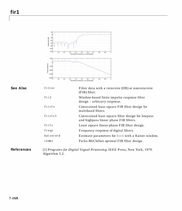
fir1
7-168
See Also
References [1] Programs for Digital Signal Processing, IEEE Press, New York, 1979.Algorithm 5.2.
0 0.1 0.2 0.3 0.4 0.5 0.6 0.7 0.8 0.9 1−2000
−1500
−1000
−500
0
500
Normalized Frequency (×π rad/sample)
Pha
se (
degr
ees)
0 0.1 0.2 0.3 0.4 0.5 0.6 0.7 0.8 0.9 1−120
−100
−80
−60
−40
−20
0
20
Normalized Frequency (×π rad/sample)
Mag
nitu
de (
dB)
filter Filter data with a recursive (IIR) or nonrecursive(FIR) filter.
fir2 Window-based finite impulse response filterdesign – arbitrary response.
fircls Constrained least square FIR filter design formultiband filters.
fircls1 Constrained least square filter design for lowpassand highpass linear phase FIR filters.
firls Least square linear-phase FIR filter design.
freqz Frequency response of digital filters.
kaiserord Estimate parameters for fir1 with a Kaiser window.
remez Parks-McClellan optimal FIR filter design.
fir2
7-169
7fir2Purpose Design a frequency sampling-based finite impulse response filter.
Syntax b = fir2(n,f,m)b = fir2(n,f,m,window)b = fir2(n,f,m,npt)b = fir2(n,f,m,npt,window)b = fir2(n,f,m,npt,lap)b = fir2(n,f,m,npt,lap,window)
Description fir2 designs frequency sampling-based digital FIR filters with arbitrarilyshaped frequency response.
Note Use fir1 for windows-based standard lowpass, bandpass, highpass,and bandstop configurations.
b = fir2(n,f,m) returns row vector b containing the n+1 coefficients of anorder n FIR filter. The frequency-magnitude characteristics of this filter matchthose given by vectors f and m:
• f is a vector of frequency points in the range from 0 to 1, where 1 correspondsto the Nyquist frequency. The first point of f must be 0 and the last point 1.The frequency points must be in increasing order.
• m is a vector containing the desired magnitude response at the pointsspecified in f.
• f and m must be the same length.
• Duplicate frequency points are allowed, corresponding to steps in thefrequency response.
Use plot(f,m) to view the filter shape.
The output filter coefficients, b, are ordered in descending powers of z.
fir2 always uses an even filter order for configurations with a passband at theNyquist frequency. This is because for odd orders, the frequency response at
b z( ) b 1( ) b 2( )z 1– b n 1+( )z n–+ + +=
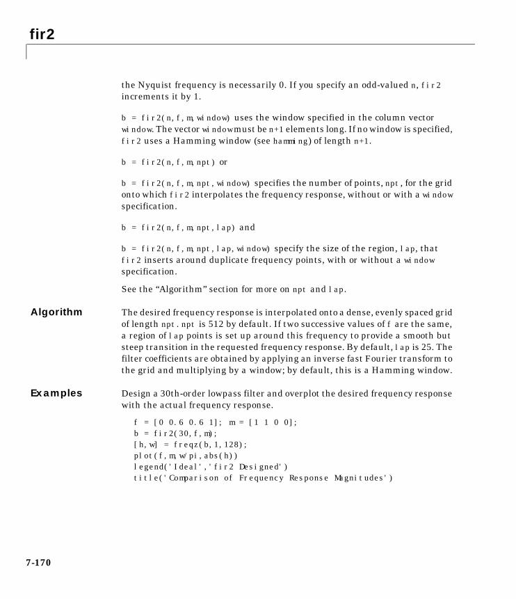
fir2
7-170
the Nyquist frequency is necessarily 0. If you specify an odd-valued n, fir2increments it by 1.
b = fir2(n,f,m,window) uses the window specified in the column vectorwindow. The vector windowmust be n+1 elements long. If no window is specified,fir2 uses a Hamming window (see hamming) of length n+1.
b = fir2(n,f,m,npt) or
b = fir2(n,f,m,npt,window) specifies the number of points, npt, for the gridonto which fir2 interpolates the frequency response, without or with a windowspecification.
b = fir2(n,f,m,npt,lap) and
b = fir2(n,f,m,npt,lap,window) specify the size of the region, lap, thatfir2 inserts around duplicate frequency points, with or without a windowspecification.
See the “Algorithm” section for more on npt and lap.
Algorithm The desired frequency response is interpolated onto a dense, evenly spaced gridof length npt. npt is 512 by default. If two successive values of f are the same,a region of lap points is set up around this frequency to provide a smooth butsteep transition in the requested frequency response. By default, lap is 25. Thefilter coefficients are obtained by applying an inverse fast Fourier transform tothe grid and multiplying by a window; by default, this is a Hamming window.
Examples Design a 30th-order lowpass filter and overplot the desired frequency responsewith the actual frequency response.
f = [0 0.6 0.6 1]; m = [1 1 0 0];b = fir2(30,f,m);[h,w] = freqz(b,1,128);plot(f,m,w/pi,abs(h))legend('Ideal','fir2 Designed')title('Comparison of Frequency Response Magnitudes')
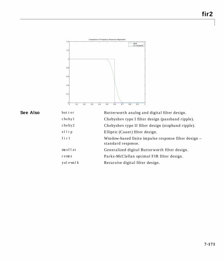
fir2
7-171
See Also
0 0.1 0.2 0.3 0.4 0.5 0.6 0.7 0.8 0.9 10
0.2
0.4
0.6
0.8
1
1.2
1.4Comparison of Frequency Response Magnitudes
Ideal fir2 Designed
butter Butterworth analog and digital filter design.
cheby1 Chebyshev type I filter design (passband ripple).
cheby2 Chebyshev type II filter design (stopband ripple).
ellip Elliptic (Cauer) filter design.
fir1 Window-based finite impulse response filter design –standard response.
maxflat Generalized digital Butterworth filter design.
remez Parks-McClellan optimal FIR filter design.
yulewalk Recursive digital filter design.

fircls
7-172
7firclsPurpose Constrained least square FIR filter design for multiband filters.
Syntax b = fircls(n,f,amp,up,lo)fircls(n,f,amp,up,lo,'design_flag')
Description b = fircls(n,f,amp,up,lo) generates a length n+1 linear phase FIR filter b.The frequency-magnitude characteristics of this filter match those given byvectors f and amp:
• f is a vector of transition frequencies in the range from 0 to 1, where 1corresponds to the Nyquist frequency. The first point of f must be 0 and thelast point 1. The frequency points must be in increasing order.
• amp is a vector describing the piecewise constant desired amplitude of thefrequency response. The length of amp is equal to the number of bands in theresponse and should be equal to length(f)-1.
• up and lo are vectors with the same length as amp. They define the upper andlower bounds for the frequency response in each band.
fircls always uses an even filter order for configurations with a passband atthe Nyquist frequency. This is because for odd orders, the frequency responseat the Nyquist frequency is necessarily 0. If you specify an odd-valued n,fircls increments it by 1.
fircls(n,f,amp,up,lo,'design_flag') enables you to monitor the filterdesign, where 'design_flag' can be:
• 'trace', for a textual display of the design error at each iteration step.
• 'plots', for a collection of plots showing the filter’s full-band magnituderesponse and a zoomed view of the magnitude response in each sub-band. Allplots are updated at each iteration step.
• 'both', for both the textual display and plots.

fircls
7-173
Examples Design an order 50 bandpass filter.
n = 50;f = [0 0.4 0.8 1];amp = [0 1 0];up = [0.02 1.02 0.01];lo = [-0.02 0.98 -0.01];b = fircls(n,f,amp,up,lo,'plots'); % Plot magnitude response
Note Normally, the lower value in the stopband will be specified as negative.By setting lo equal to 0 in the stopbands, a nonnegative frequency responseamplitude can be obtained. Such filters can be spectrally factored to obtainminimum phase filters.
Algorithm The algorithm is a multiple exchange algorithm that uses Lagrangemultipliers and Kuhn-Tucker conditions on each iteration.
0 0.2 0.4 0.6 0.8 1 1.2 1.4-2
0
2
0 0.05 0.1 0.15 0.2 0.25 0.3 0.35 0.4
-0.02
0
0.02
Ban
d #1
0.4 0.45 0.5 0.55 0.6 0.65 0.7 0.75 0.8
0.98
1
1.02
Ban
d #2
0.8 0.85 0.9 0.95 1
-0.01
0
0.01
Ban
d #3
Frequency

fircls
7-174
See Also
References [1] Selesnick, I.W., M. Lang, and C.S. Burrus, “Constrained Least SquareDesign of FIR Filters without Specified Transition Bands,” Proceedings of theIEEE Int. Conf. Acoust., Speech, Signal Processing, Vol. 2 (May 1995),pp. 1260-1263.
[2] Selesnick, I.W., M. Lang, and C.S. Burrus. “Constrained Least SquareDesign of FIR Filters without Specified Transition Bands.” IEEE Transactionson Signal Processing, Vol. 44, No. 8 (August 1996).
fircls1 Constrained least square filter design for lowpassand highpass linear phase FIR filters.
firls Least square linear-phase FIR filter design.
remez Parks-McClellan optimal FIR filter design.

fircls1
7-175
7fircls1Purpose Constrained least square filter design for lowpass and highpass linear phaseFIR filters.
Syntax b = fircls1(n,wo,dp,ds)b = fircls1(n,wo,dp,ds,'high')b = fircls1(n,wo,dp,ds,wt)b = fircls1(n,wo,dp,ds,wt,'high')b = fircls1(n,wo,dp,ds,wp,ws,k)b = fircls1(n,wo,dp,ds,wp,ws,k,'high')b = fircls1(n,wo,dp,ds,...,'design_flag')
Description b = fircls1(n,wo,dp,ds) generates a lowpass FIR filter b, where n+1 is thefilter length, wo is the normalized cutoff frequency in the range between 0 and 1(where 1 corresponds to the Nyquist frequency), dp is the maximum passbanddeviation from 1 (passband ripple), and ds is the maximum stopband deviationfrom 0 (stopband ripple).
b = fircls1(n,wo,dp,ds,'high') generates a highpass FIR filter b. fircls1always uses an even filter order for the highpass configuration. This is becausefor odd orders, the frequency response at the Nyquist frequency isnecessarily 0. If you specify an odd-valued n, fircls1 increments it by 1.
b = fircls1(n,wo,dp,ds,wt) and
b = fircls1(n,wo,dp,ds,wt,'high') specifies a frequency wt above which(for wt > wo) or below which (for wt < wo) the filter is guaranteed to meet thegiven band criterion. This will help you design a filter that meets a passbandor stopband edge requirement. There are four cases:
• Lowpass:
- 0 < wt < wo < 1: the amplitude of the filter is within dp of 1 over thefrequency range 0 < ω < wt.
- 0 < wo < wt < 1: the amplitude of the filter is within ds of 0 over thefrequency range wt < ω < 1.

fircls1
7-176
• Highpass:
- 0 < wt < wo < 1: the amplitude of the filter is within ds of 0 over thefrequency range 0 < ω < wt.
- 0 < wo < wt < 1: the amplitude of the filter is within dp of 1 over thefrequency range wt < ω < 1.
b = fircls1(n,wo,dp,ds,wp,ws,k) generates a lowpass FIR filter b with aweighted function, where n+1 is the filter length, wo is the normalized cutofffrequency, dp is the maximum passband deviation from 1 (passband ripple), andds is the maximum stopband deviation from 0 (stopband ripple). wp is thepassband edge of the L2 weight function and ws is the stopband edge of the L2weight function, where wp < wo < ws. k is the ratio (passband L2 error)/(stopbandL2 error)
b = fircls1(n,wo,dp,ds,wp,ws,k,'high') generates a highpass FIR filter bwith a weighted function, where ws < wo < wp.
b = fircls1(n,wo,dp,ds,...,'design_flag') enables you to monitor thefilter design, where 'design_flag' can be:
• 'trace', for a textual display of the design table used in the design
• 'plots', for plots of the filter’s magnitude, group delay, and zeros and poles
• 'both', for both the textual display and plots
Note In the design of very narrow band filters with small dp and ds, theremay not exist a filter of the given length that meets the specifications.
kA ω( ) D ω( )– 2 ωd
0
wp
A ω( ) D ω( )– 2 ωdws
π
------------------------------------------------------=
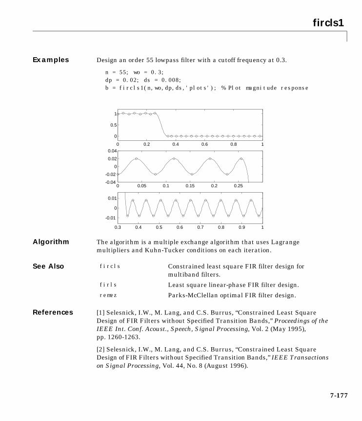
fircls1
7-177
Examples Design an order 55 lowpass filter with a cutoff frequency at 0.3.
n = 55; wo = 0.3;dp = 0.02; ds = 0.008;b = fircls1(n,wo,dp,ds,'plots'); % Plot magnitude response
Algorithm The algorithm is a multiple exchange algorithm that uses Lagrangemultipliers and Kuhn-Tucker conditions on each iteration.
See Also
References [1] Selesnick, I.W., M. Lang, and C.S. Burrus, “Constrained Least SquareDesign of FIR Filters without Specified Transition Bands,” Proceedings of theIEEE Int. Conf. Acoust., Speech, Signal Processing, Vol. 2 (May 1995),pp. 1260-1263.
[2] Selesnick, I.W., M. Lang, and C.S. Burrus, “Constrained Least SquareDesign of FIR Filters without Specified Transition Bands,” IEEE Transactionson Signal Processing, Vol. 44, No. 8 (August 1996).
0 0.2 0.4 0.6 0.8 1
0
0.5
1
0 0.05 0.1 0.15 0.2 0.25-0.04
-0.02
0
0.02
0.04
0.3 0.4 0.5 0.6 0.7 0.8 0.9 1
-0.01
0
0.01
fircls Constrained least square FIR filter design formultiband filters.
firls Least square linear-phase FIR filter design.
remez Parks-McClellan optimal FIR filter design.

firls
7-178
7firlsPurpose Least square linear-phase FIR filter design.
Syntax b = firls(n,f,a)b = firls(n,f,a,w)b = firls(n,f,a,'ftype')b = firls(n,f,a,w,'ftype')
Description firls designs a linear-phase FIR filter that minimizes the weighted,integrated squared error between an ideal piecewise linear function and themagnitude response of the filter over a set of desired frequency bands.
b = firls(n,f,a) returns row vector b containing the n+1 coefficients of theorder n FIR filter whose frequency-amplitude characteristics approximatelymatch those given by vectors f and a. The output filter coefficients, or “taps,”in b obey the symmetry relation.
These are type I (n odd) and type II (n even) linear-phase filters. Vectors f and aspecify the frequency-amplitude characteristics of the filter:
• f is a vector of pairs of frequency points, specified in the range between 0and 1, where 1 corresponds to the Nyquist frequency. The frequencies mustbe in increasing order. Duplicate frequency points are allowed and, in fact,can be used to design a filter exactly the same as those returned by the fir1and fir2 functions with a rectangular or boxcar window.
• a is a vector containing the desired amplitude at the points specified in f.
The desired amplitude function at frequencies between pairs of points(f(k), f(k+1)) for k odd is the line segment connecting the points (f(k), a(k))and (f(k+1), a(k+1)).
The desired amplitude function at frequencies between pairs of points(f(k), f(k+1)) for k even is unspecified. These are transition or “don’t care”regions.
• f and a are the same length. This length must be an even number.
firls always uses an even filter order for configurations with a passband atthe Nyquist frequency. This is because for odd orders, the frequency response
b k( ) b n 2 k–+( ) k 1= … n 1+, , ,=

firls
7-179
at the Nyquist frequency is necessarily 0. If you specify an odd-valued n, firlsincrements it by 1.
The figure below illustrates the relationship between the f and a vectors indefining a desired amplitude response.
b = firls(n,f,a,w) uses the weights in vector w to weight the fit in eachfrequency band. The length of w is half the length of f and a, so there is exactlyone weight per band.
b = firls(n,f,a,'ftype') and
b = firls(n,f,a,w,'ftype') specify a filter type, where 'ftype' is:
• 'hilbert' for linear-phase filters with odd symmetry (type III and type IV).The output coefficients in b obey the relation b(k) = -b(n+2-k),k = 1, ... , n + 1. This class of filters includes the Hilbert transformer, whichhas a desired amplitude of 1 across the entire band.
• 'differentiator' for type III and type IV filters, using a special weightingtechnique. For nonzero amplitude bands, the integrated squared error has aweight of (1/f)2 so that the error at low frequencies is much smaller than athigh frequencies. For FIR differentiators, which have an amplitudecharacteristic proportional to frequency, the filters minimize the relativeintegrated squared error (the integral of the square of the ratio of the errorto the desired amplitude).
1.0
0.0
Desired amplituderesponse (a)
Normalizedfrequency (f)
0.5
"Don't care"/transition regions
f = [0 .3 .4 .6 .7 .9]a = [0 1 0 0 .5 .5]
0.1 0.2 0.3 0.4 0.5 0.6 0.70.0 0.8 0.9 1.0 (Nyquist)
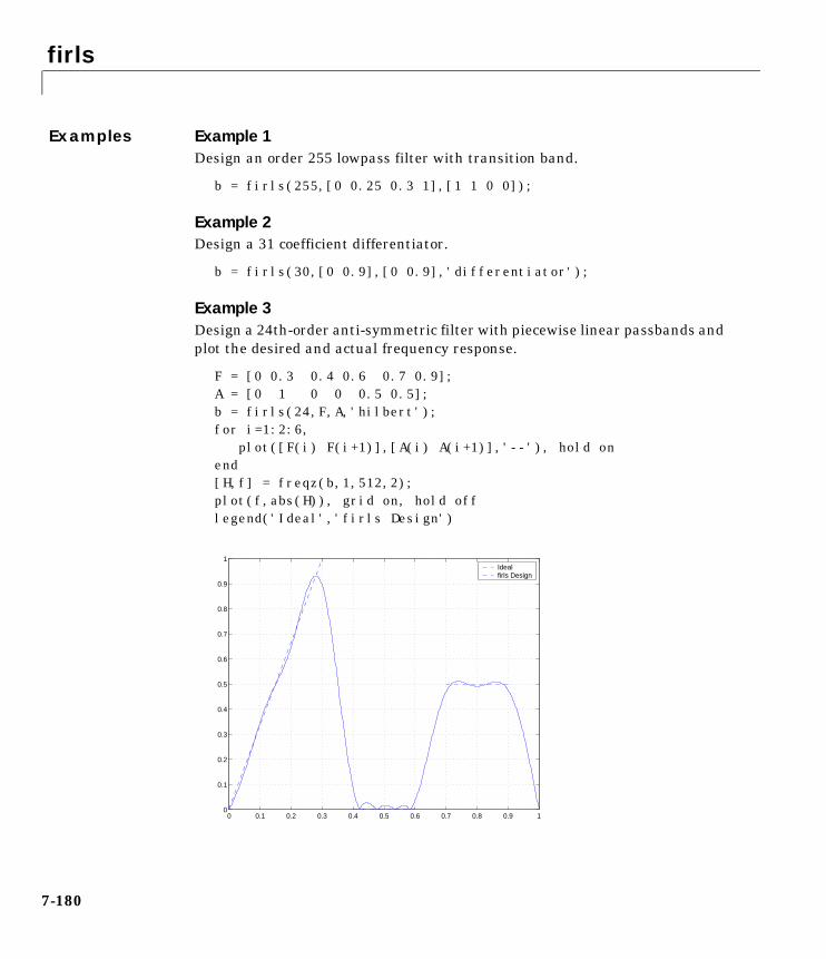
firls
7-180
Examples Example 1Design an order 255 lowpass filter with transition band.
b = firls(255,[0 0.25 0.3 1],[1 1 0 0]);
Example 2Design a 31 coefficient differentiator.
b = firls(30,[0 0.9],[0 0.9],'differentiator');
Example 3Design a 24th-order anti-symmetric filter with piecewise linear passbands andplot the desired and actual frequency response.
F = [0 0.3 0.4 0.6 0.7 0.9]; A = [0 1 0 0 0.5 0.5];b = firls(24,F,A,'hilbert');for i=1:2:6, plot([F(i) F(i+1)],[A(i) A(i+1)],'--'), hold onend[H,f] = freqz(b,1,512,2);plot(f,abs(H)), grid on, hold offlegend('Ideal','firls Design')
0 0.1 0.2 0.3 0.4 0.5 0.6 0.7 0.8 0.9 10
0.1
0.2
0.3
0.4
0.5
0.6
0.7
0.8
0.9
1Ideal firls Design
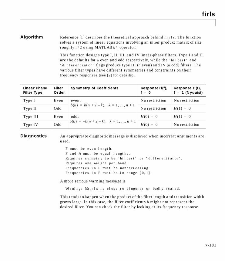
firls
7-181
Algorithm Reference [1] describes the theoretical approach behind firls. The functionsolves a system of linear equations involving an inner product matrix of sizeroughly n/2 using MATLAB’s \ operator.
This function designs type I, II, III, and IV linear-phase filters. Type I and IIare the defaults for n even and odd respectively, while the 'hilbert' and'differentiator' flags produce type III (n even) and IV (n odd) filters. Thevarious filter types have different symmetries and constraints on theirfrequency responses (see [2] for details).
Diagnostics An appropriate diagnostic message is displayed when incorrect arguments areused.
F must be even length.F and A must be equal lengths.Requires symmetry to be 'hilbert' or 'differentiator'.Requires one weight per band.Frequencies in F must be nondecreasing.Frequencies in F must be in range [0,1].
A more serious warning message is
Warning: Matrix is close to singular or badly scaled.
This tends to happen when the product of the filter length and transition widthgrows large. In this case, the filter coefficients b might not represent thedesired filter. You can check the filter by looking at its frequency response.
Linear Phase Filter Type
Filter Order
Symmetry of Coefficients Response H(f), f = 0
Response H(f), f = 1 (Nyquist)
Type I Even even: No restriction No restriction
Type II Odd No restriction H(1) = 0
Type III Even odd: H(0) = 0 H(1) = 0
Type IV Odd H(0) = 0 No restriction
b k( ) b n 2 k–+( ) k 1= … n 1+, , ,=
b k( ) b– n 2 k–+( ) k 1= … n 1+, , ,=

firls
7-182
See Also
References [1] Parks, T.W., and C.S. Burrus, Digital Filter Design, John Wiley & Sons,1987, pp. 54-83.
[2] Oppenheim, A.V., and R.W. Schafer, Discrete-Time Signal Processing,Prentice-Hall, 1989, pp. 256-266.
fir1 Window-based finite impulse response filter design –standard response.
fir2 Window-based finite impulse response filter design –arbitrary response.
firrcos Raised cosine FIR filter design.
remez Parks-McClellan optimal FIR filter design.
firrcos
7-183
7firrcosPurpose Raised cosine FIR filter design.
b = firrcos(n,F0,df,fs)b = firrcos(n,F0,df,fs,'bandwidth')b = firrcos(n,F0,df)b = firrcos(n,F0,r,fs,'rolloff')b = firrcos(...,'type')b = firrcos(...,'type',delay)b = firrcos(...,'type',delay,window)[b,a] = firrcos(...)
Description b = firrcos(n,F0,df,fs) or, equivalently,
b = firrcos(n,F0,df,fs,'bandwidth') returns an order n lowpasslinear-phase FIR filter with a raised cosine transition band. The filter hascutoff frequency F0, transition bandwidth df, and sampling frequency fs, all inhertz. df must be small enough so that F0 ± df/2 is between 0 and fs/2. Thecoefficients in b are normalized so that the nominal passband gain is alwaysequal to 1. Specify fs as the empty vector [] to use the default value fs = 2.
b = firrcos(n,F0,df) uses a default sampling frequency of fs = 2.
b = firrcos(n,F0,r,fs,'rolloff') interprets the third argument, r, as therolloff factor instead of the transition bandwidth, df. r must be in the range[0,1].
b = firrcos(...,'type') designs either a normal raised cosine filter or asquare root raised cosine filter according to how you specify of the string'type'. Specify 'type' as:
• 'normal', for a regular raised cosine filter. This is the default, and is also ineffect when the 'type' argument is left empty, [].
• 'sqrt', for a square root raised cosine filter.
b = firrcos(...,'type',delay) specifies an integer delay in the range[0,n+1]. The default is n/2 for even n and (n+1)/2 for odd n.
b = firrcos(...,'type',delay,window) applies a length n+1 window to thedesigned filter to reduce the ripple in the frequency response. window must bea length n+1 column vector. If no window is specified, a boxcar (rectangular)

firrcos
7-184
window is used. Care must be exercised when using a window with a delayother than the default.
[b,a] = firrcos(...) always returns a = 1.
Examples Design an order 20 raised cosine FIR filter with cutoff frequency 0.25 of theNyquist frequency and a transition bandwidth of 0.25.
h = firrcos(20,0.25,0.25);freqz(h,1)
See Also
0 0.1 0.2 0.3 0.4 0.5 0.6 0.7 0.8 0.9 1−700
−600
−500
−400
−300
−200
−100
0
Normalized Frequency (×π rad/sample)
Pha
se (
degr
ees)
0 0.1 0.2 0.3 0.4 0.5 0.6 0.7 0.8 0.9 1−120
−100
−80
−60
−40
−20
0
20
Normalized Frequency (×π rad/sample)
Mag
nitu
de (
dB)
fir1 Window-based finite impulse response filter design –standard response.
fir2 Window-based finite impulse response filter design –arbitrary response.
firls Least square linear-phase FIR filter design.
remez Parks-McClellan optimal FIR filter design.
freqs
7-185
7freqsPurpose Frequency response of analog filters.
Syntax h = freqs(b,a,w)[h,w] = freqs(b,a)[h,w] = freqs(b,a,n)freqs(b,a)
Description freqs returns the complex frequency response H(jω) (Laplace transform) of ananalog filter
given the numerator and denominator coefficients in vectors b and a.
h = freqs(b,a,w) returns the complex frequency response of the analog filterspecified by coefficient vectors b and a. freqs evaluates the frequency responsealong the imaginary axis in the complex plane at the frequencies specified inreal vector w.
[h,w] = freqs(b,a) automatically picks a set of 200 frequency points w onwhich to compute the frequency response h.
[h,w] = freqs(b,a,n) picks n frequencies on which to compute the frequencyresponse h.
freqs with no output arguments plots the magnitude and phase responseversus frequency in the current figure window.
freqs works only for real input systems and positive frequencies.
Examples Find and graph the frequency response of the transfer function given by
a = [1 0.4 1];b = [0.2 0.3 1];w = logspace(-1,1);freqs(b,a,w)
H s( )B s( )A s( )----------- b 1( )snb b 2( )snb 1– b nb 1+( )+ + +
a 1( )sna a 2( )sna 1– a na 1+( )+ + +-------------------------------------------------------------------------------------------------= =
H s( )0.2s2 0.3s 1+ +
s2 0.4s 1+ +-----------------------------------------=
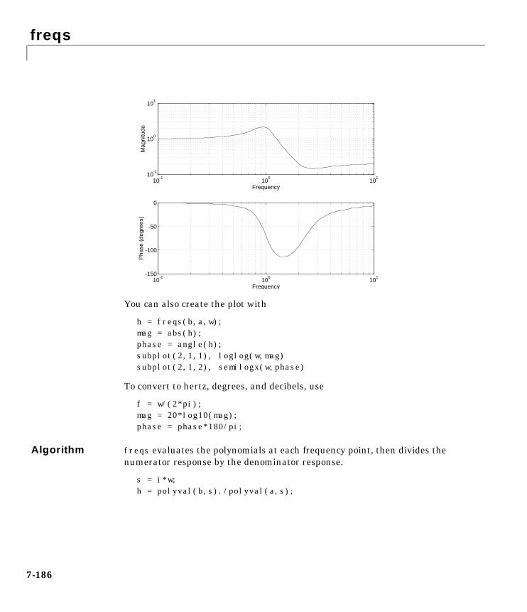
freqs
7-186
You can also create the plot with
h = freqs(b,a,w);mag = abs(h);phase = angle(h);subplot(2,1,1), loglog(w,mag)subplot(2,1,2), semilogx(w,phase)
To convert to hertz, degrees, and decibels, use
f = w/(2*pi);mag = 20*log10(mag);phase = phase*180/pi;
Algorithm freqs evaluates the polynomials at each frequency point, then divides thenumerator response by the denominator response.
s = i*w;h = polyval(b,s)./polyval(a,s);
10-1
100
101
10-1
100
101
Frequency
Mag
nitu
de
10-1
100
101
-150
-100
-50
0
Frequency
Pha
se (
degr
ees)

freqs
7-187
See Also abs Absolute value (magnitude).
angle Phase angle.
freqz Frequency response of digital filters.
invfreqs Continuous-time (analog) filter identification fromfrequency data.
logspace Generate logarithmically spaced vectors (see theMATLAB documentation).
polyval Polynomial evaluation (see the MATLABdocumentation).
freqspace
7-188
7freqspacePurpose Frequency spacing for frequency response.
Syntax f = freqspace(n)f = freqspace(n,'whole')[f1,f2] = freqspace(n)[f1,f2] = freqspace([m n])[x1,y1] = freqspace(n,'meshgrid')[x1,y1] = freqspace([m n],'meshgrid')
Description freqspace returns the implied frequency range for equally spaced frequencyresponses. This is useful when creating frequency vectors for use with freqz.
f = freqspace(n) returns the frequency vector f assuming n evenly spacedpoints around the unit circle. For n even or odd, f is (0:2/n:1). For n even,freqspace returns (n + 2)/2 points. For N odd, it returns (n + 1)/2 points.
f = freqspace(n,'whole') returns n evenly spaced points around the wholeunit circle. In this case, f is 0:2/n:2*(n-1)/n.
[f1,f2] = freqspace(n) returns the two-dimensional frequency vectors f1and f2 for an n-by-n matrix. For n odd, both f1 and f2 are[-1 + 1/n:2/n:1-1/n]. For n even, both f1 and f2 are [-1:2/n:1-2/n].
[f1,f2] = freqspace([m n]) returns the two-dimensional frequency vectorsf1 and f2 for an m-by-n matrix.
[x1,y1] = freqspace(n,'meshgrid') and
[x1,y1] = freqspace([m n],'meshgrid') are equivalent to
[f1,f2] = freqspace(...);[x1,y1] = meshgrid(f1,f2);
See the MATLAB documentation for details on the meshgrid function.
See Also freqz Compute the frequency response of digital filters.
invfreqz Discrete-time filter identification from frequencydata.

freqz
7-189
7freqzPurpose Compute the frequency response of digital filters.
Syntax [h,w]= freqz(b,a,n)h = freqz(b,a,w)[h,w] = freqz(b,a,n,'whole')[h,w,units] = freqz(b,a,...)[h,f] = freqz(b,a,n,fs)h = freqz(b,a,f,fs)[h,f] = freqz(b,a,n,'whole',fs)[h,f,units] = freqz(b,a,n,'whole',fs)freqz(b,a,...)
Description [h,w] = freqz(b,a,n) returns the frequency response vector h and thecorresponding frequency vector w for the digital filter whose transfer functionis determined by the (real or complex) numerator and denominatorpolynomials represented in the vectors b and a, respectively. The vectors hand w are both of length n. The frequency vector w has values ranging from 0 to π radians per sample. When you don’t specify the integer n, or you specify it asthe empty vector [], the frequency response is calculated using the defaultvalue of 512 samples.
h = freqz(b,a,w) returns the frequency response vector h calculated at thefrequencies (in radians per sample) supplied by the vector w. The vector w canhave any length.
[h,w] = freqz(b,a,n,'whole') uses n sample points around the entire unitcircle to calculate the frequency response. The frequency vector w has length nand has values ranging from 0 to 2π radians per sample.
[h,w,units] = freqz(b,a,...) returns the optional string argument units,specifying the units for the frequency vector w. The string returned in units is'rad/sample', denoting radians per sample.
[h,f] = freqz(b,a,n,fs) returns the frequency response vector h and thecorresponding frequency vector f for the digital filter whose transfer functionis determined by the (real or complex) numerator and denominatorpolynomials represented in the vectors b and a, respectively. The vectors hand f are both of length n. For this syntax, the frequency response is calculated
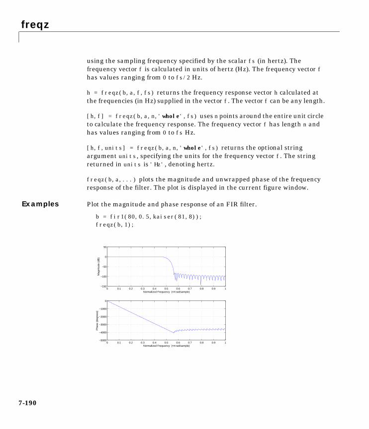
freqz
7-190
using the sampling frequency specified by the scalar fs (in hertz). Thefrequency vector f is calculated in units of hertz (Hz). The frequency vector fhas values ranging from 0 to fs/2 Hz.
h = freqz(b,a,f,fs) returns the frequency response vector h calculated atthe frequencies (in Hz) supplied in the vector f. The vector f can be any length.
[h,f] = freqz(b,a,n,'whole',fs) uses n points around the entire unit circleto calculate the frequency response. The frequency vector f has length n andhas values ranging from 0 to fs Hz.
[h,f,units] = freqz(b,a,n,'whole',fs) returns the optional stringargument units, specifying the units for the frequency vector f. The stringreturned in units is 'Hz', denoting hertz.
freqz(b,a,...) plots the magnitude and unwrapped phase of the frequencyresponse of the filter. The plot is displayed in the current figure window.
Examples Plot the magnitude and phase response of an FIR filter.
b = fir1(80,0.5,kaiser(81,8));freqz(b,1);
0 0.1 0.2 0.3 0.4 0.5 0.6 0.7 0.8 0.9 1−5000
−4000
−3000
−2000
−1000
0
Normalized Frequency (×π rad/sample)
Pha
se (
degr
ees)
0 0.1 0.2 0.3 0.4 0.5 0.6 0.7 0.8 0.9 1−150
−100
−50
0
50
Normalized Frequency (×π rad/sample)
Mag
nitu
de (
dB)
freqz
7-191
Remarks It is best to choose a power of two for the third input argument n, because freqzuses an FFT algorithm to calculate the frequency response. See the referencedescription of fft for more information.
Algorithm The frequency response [1] of a digital filter can be interpreted as the transferfunction evaluated at z = ejω. You can always write a rational transfer functionin the following form.
freqz determines the transfer function from the (real or complex) numeratorand denominator polynomials you specify, and returns the complex frequencyresponse H(ejω) of a digital filter. The frequency response is evaluated atsample points determined by the syntax that you use.
freqz generally uses an FFT algorithm to compute the frequency responsewhenever you don’t supply a vector of frequencies as an input argument. Itcomputes the frequency response as the ratio of the transformed numeratorand denominator coefficients, padded with zeros to the desired length.
When you do supply a vector of frequencies as an input argument, then freqzevaluates the polynomials at each frequency point using Horner’s method ofnested polynomial evaluation [1], dividing the numerator response by thedenominator response.
H z( )B z( )A z( )----------- b 1( ) b 2( )z 1– b nb 1+( )z nb–+ + +
a 1( ) a 2( )z 1– a na 1+( )z na–+ + +--------------------------------------------------------------------------------------------= =
freqz
7-192
See Also
References [1] Oppenheim, A.V., and R.W. Schafer, Discrete-Time Signal Processing,Prentice-Hall, 1989, pp. 203-205.
abs Compute the absolute value (magnitude).
angle Compute the phase angle.
fft Compute the one-dimensional fast Fouriertransform.
filter Filter data.
freqs Compute the frequency response of analog filters.
freqzplot Plot the frequency response of a digital filter.
impz Compute the impulse response of digital filters.
invfreqz Identify discrete-time filter parameters fromfrequency data.
logspace Generate logarithmically spaced vectors (see theMATLAB documentation).
freqzplot
7-193
7freqzplotPurpose Plot frequency response data.
Syntax freqzplot(h,w)freqzplot(h,w,s)
Description freqzplot(h,w) plots the frequency response data contained in h at thefrequencies specified in the vector w, where h can be either a vector or a matrix.w must be a vector whose length is the number of rows in h. The data in h isplotted versus frequency w on two plots:
• The magnitude of h is plotted in dB.
• The phase of h is plotted in degrees.
The units for frequency on the plots are in radians per sample. If h is a matrix,the frequency responses of each column of h is plotted.
freqzplot(h,w,s) specifies a structure of plotting options, s, with thefollowing fields:
• s.xunits – a string specifying the frequency axis units. The contents ofs.xunits can be one of the following:
- 'rad/sample' (default)
- 'Hz'
- 'kHz'
- 'MHz'
- 'GHz'
- A user-specified string
• s.yunits – a string specifying the vertical axis units. The contents ofs.yunits can be one of the following:
- 'dB' (default)
- 'linear'
- 'squared'
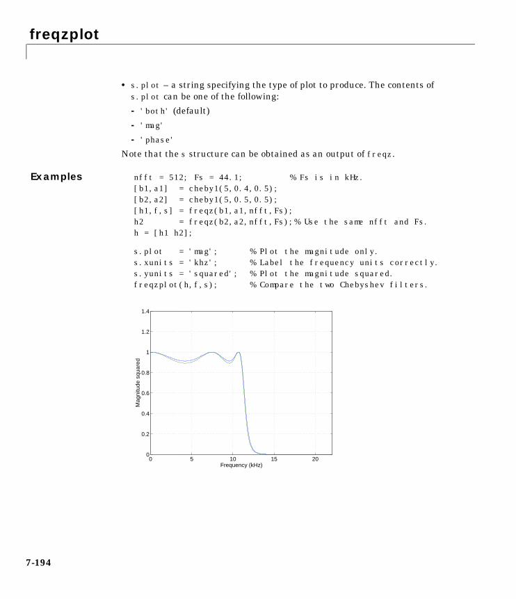
freqzplot
7-194
• s.plot – a string specifying the type of plot to produce. The contents ofs.plot can be one of the following:
- 'both' (default)
- 'mag'
- 'phase'
Note that the s structure can be obtained as an output of freqz.
Examples nfft = 512; Fs = 44.1; % Fs is in kHz.[b1,a1] = cheby1(5,0.4,0.5);[b2,a2] = cheby1(5,0.5,0.5);[h1,f,s] = freqz(b1,a1,nfft,Fs);h2 = freqz(b2,a2,nfft,Fs);% Use the same nfft and Fs.h = [h1 h2];
s.plot = 'mag'; % Plot the magnitude only.s.xunits = 'khz'; % Label the frequency units correctly.s.yunits = 'squared'; % Plot the magnitude squared.freqzplot(h,f,s); % Compare the two Chebyshev filters.
0 5 10 15 200
0.2
0.4
0.6
0.8
1
1.2
1.4
Frequency (kHz)
Mag
nitu
de s
quar
ed

freqzplot
7-195
See Also freqz Compute and plot the frequency response of a filter.
grpdelay Compute the average filter delay.
psdplot Plot power spectral density (PSD) data.
gauspuls
7-196
7gauspulsPurpose Generate a Gaussian-modulated sinusoidal pulse.
Syntax yi = gauspuls(t,fc,bw)yi = gauspuls(t,fc,bw,bwr)[yi,yq] = gauspuls(...)[yi,yq,ye] = gauspuls(...)tc = gauspuls('cutoff',fc,bw,bwr,tpe)
Description gauspuls generates Gaussian-modulated sinusoidal pulses.
yi = gauspuls(t,fc,bw) returns a unity-amplitude Gaussian RF pulse at thetimes indicated in array t, with a center frequency fc in hertz and a fractionalbandwidth bw, which must be greater than 0. The default value for fc is1000 Hz and for bw is 0.5.
yi = gauspuls(t,fc,bw,bwr) returns a unity-amplitude Gaussian RF pulsewith a fractional bandwidth of bw as measured at a level of bwr dB with respectto the normalized signal peak. The fractional bandwidth reference level bwr must be less than 0, because it indicates a reference level less than the peak(unity) envelope amplitude. The default value for bwr is -6 dB.
[yi,yq] = gauspuls(...) returns both the in-phase and quadrature pulses.
[yi,yq,ye] = gauspuls(...) returns the RF signal envelope.
tc = gauspuls('cutoff',fc,bw,bwr,tpe) returns the cutoff time tc (greaterthan or equal to 0) at which the trailing pulse envelope falls below tpe dB withrespect to the peak envelope amplitude. The trailing pulse envelope level tpe must be less than 0, because it indicates a reference level less than the peak(unity) envelope amplitude. The default value for tpe is -60 dB.
Remarks Default values are substituted for empty or omitted trailing input arguments.

gauspuls
7-197
Examples Plot a 50 kHz Gaussian RF pulse with 60% bandwidth, sampled at a rate of1 MHz. Truncate the pulse where the envelope falls 40 dB below the peak.
tc = gauspuls('cutoff',50e3,0.6,[],-40); t = -tc : 1e-6 : tc; yi = gauspuls(t,50e3,0.6); plot(t,yi)
See Also
-4 -2 0 2 4
x 10-5
-0.8
-0.6
-0.4
-0.2
0
0.2
0.4
0.6
0.8
1
chirp Generate a swept-frequency cosine.
cos Compute the cosine of vector/matrix elements (seethe MATLAB documentation).
diric Compute the Dirichlet or periodic sinc function.
pulstran Generate a pulse train.
rectpuls Generate a sampled aperiodic rectangle.
sawtooth Generate a sawtooth or triangle wave.
sin Compute the sine of vector/matrix elements (see theMATLAB documentation).
sinc Compute the sinc or sin(πt)/πt function.
square Generate a square wave.
tripuls Generate a sampled aperiodic triangle.
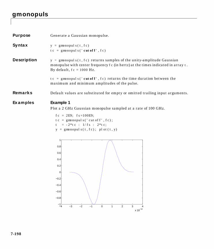
gmonopuls
7-198
7gmonopulsPurpose Generate a Gaussian monopulse.
Syntax y = gmonopuls(t,fc)tc = gmonopuls('cutoff',fc)
Description y = gmonopuls(t,fc) returns samples of the unity-amplitude Gaussianmonopulse with center frequency fc (in hertz) at the times indicated in array t.By default, fc = 1000 Hz.
tc = gmonopuls('cutoff',fc) returns the time duration between themaximum and minimum amplitudes of the pulse.
Remarks Default values are substituted for empty or omitted trailing input arguments.
Examples Example 1Plot a 2 GHz Gaussian monopulse sampled at a rate of 100 GHz.
fc = 2E9; fs=100E9;tc = gmonopuls('cutoff',fc);t = -2*tc : 1/fs : 2*tc;y = gmonopuls(t,fc); plot(t,y)
−4 −3 −2 −1 0 1 2 3 4
x 10−10
−1
−0.8
−0.6
−0.4
−0.2
0
0.2
0.4
0.6
0.8
1

gmonopuls
7-199
Example 2Construct a pulse train from the monopulse of Example 1 using a spacing of7.5 ns.
fc = 2E9; fs=100E9; % center freq, sample freqD = [2.5 10 17.5]' * 1e-9; % pulse delay timestc = gmonopuls('cutoff',fc); % width of each pulset = 0 : 1/fs : 150*tc; % signal evaluation timeyp = pulstran(t,D,@gmonopuls,fc);plot(t,yp)
See Also
0 0.5 1 1.5 2 2.5
x 10−8
−1
−0.8
−0.6
−0.4
−0.2
0
0.2
0.4
0.6
0.8
1
chirp Generate a swept-frequency cosine.
gauspuls Generate a Gaussian-modulated sinusoidal pulse.
pulstran Generate a pulse train.
rectpuls Generate a sampled aperiodic rectangle.
tripuls Generate a sampled aperiodic triangle.
grpdelay
7-200
7grpdelayPurpose Compute the average filter delay (group delay).
Syntax [gd,w] = grpdelay(b,a,n)[gd,f] = grpdelay(b,a,n,fs)[gd,w] = grpdelay(b,a,n,'whole')[gd,f] = grpdelay(b,a,n,'whole',fs)gd = grpdelay(b,a,w)gd = grpdelay(b,a,f,fs)grpdelay(b,a)
Description The group delay of a filter is a measure of the average delay of the filter as afunction of frequency. It is the negative first derivative of the phase responseof the filter. If the complex frequency response of a filter is , then thegroup delay is
where ω is frequency and θ is the phase angle of .
[gd,w] = grpdelay(b,a,n) returns the n-point group delay, , of thedigital filter
given the numerator and denominator coefficients in vectors b and a. grpdelayreturns both gd, the group delay, and w, a vector containing the n frequencypoints in radians. grpdelay evaluates the group delay at n points equallyspaced around the upper half of the unit circle, so w contains n points between0 and π.
[gd,f] = grpdelay(b,a,n,fs) specifies a positive sampling frequency fs inhertz. It returns a length n vector f containing the actual frequency points atwhich the group delay is calculated, also in hertz. f contains n points between0 and fs/2.
H ejω( )
τg ω( )dθ ω( )
dω---------------–=
H ejω( )
τg ω( )
H z( )B z( )A z( )----------- b 1( ) b 2( )z 1– b nb 1+( )z nb–+ + +
a 1( ) a 2( )z 1– a na 1+( )z na–+ + +--------------------------------------------------------------------------------------------= =
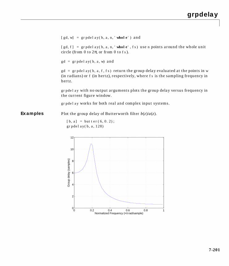
grpdelay
7-201
[gd,w] = grpdelay(b,a,n,'whole') and
[gd,f] = grpdelay(b,a,n,'whole',fs) use n points around the whole unitcircle (from 0 to 2π, or from 0 to fs).
gd = grpdelay(b,a,w) and
gd = grpdelay(b,a,f,fs) return the group delay evaluated at the points in w(in radians) or f (in hertz), respectively, where fs is the sampling frequency inhertz.
grpdelay with no output arguments plots the group delay versus frequency inthe current figure window.
grpdelay works for both real and complex input systems.
Examples Plot the group delay of Butterworth filter b(z)/a(z).
[b,a] = butter(6,0.2);grpdelay(b,a,128)
0 0.2 0.4 0.6 0.8 10
2
4
6
8
10
12
Normalized Frequency (×π rad/sample)
Gro
up d
elay
(sa
mpl
es)

grpdelay
7-202
Plot both the group and phase delays of a system on the same graph.
gd = grpdelay(b,a,512);gd(1) = []; % Avoid NaNs[h,w] = freqz(b,a,512); h(1) = []; w(1) = [];pd = -unwrap(angle(h))./w;plot(w,gd,w,pd,':')xlabel('Frequency (rad/sec)'); grid;legend('Group Delay','Phase Delay');
Algorithm grpdelay multiplies the filter coefficients by a unit ramp. After Fouriertransformation, this process corresponds to differentiation.
See Also
0 0.5 1 1.5 2 2.5 3 3.5−6
−4
−2
0
2
4
6
8
10
12
Frequency (rad/sec)
Group DelayPhase Delay
cceps Implement complex cepstral analysis.
fft Compute the frequency one-dimensional fast Fouriertransform.
freqz Compute the frequency response of digital filters.
hilbert Compute the Hilbert transform.
icceps Compute the inverse complex cepstrum.
rceps Real cepstrum and minimum phase reconstruction.
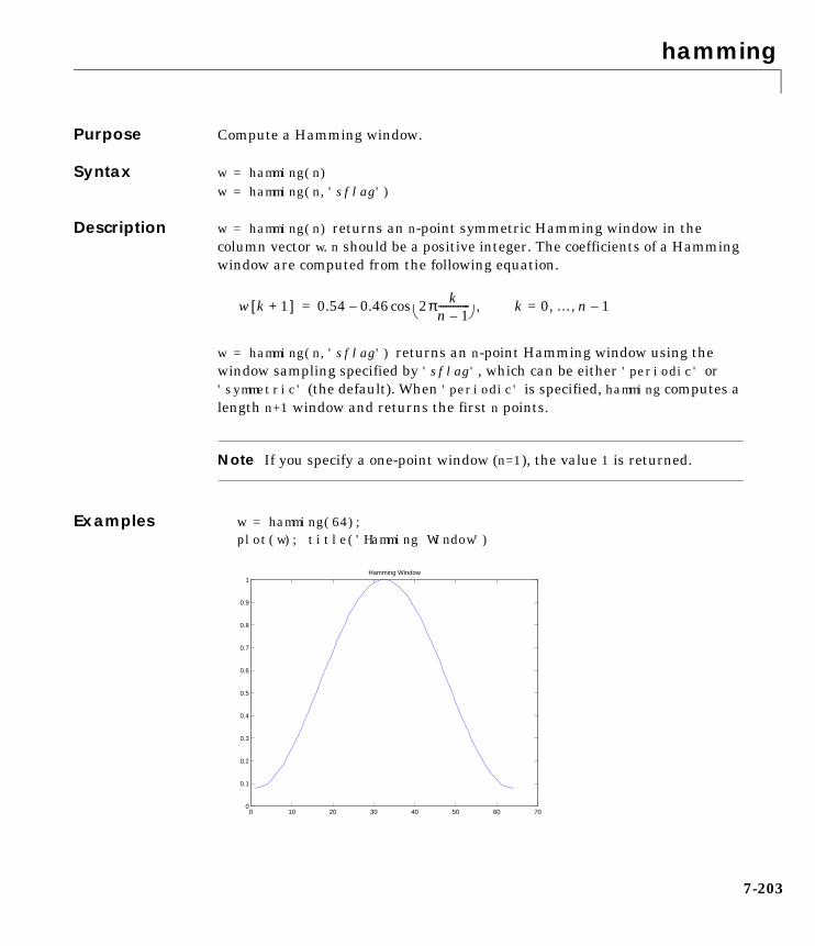
hamming
7-203
7hammingPurpose Compute a Hamming window.
Syntax w = hamming(n)w = hamming(n,'sflag')
Description w = hamming(n) returns an n-point symmetric Hamming window in thecolumn vector w. n should be a positive integer. The coefficients of a Hammingwindow are computed from the following equation.
w = hamming(n,'sflag') returns an n-point Hamming window using thewindow sampling specified by 'sflag', which can be either 'periodic' or'symmetric' (the default). When 'periodic' is specified, hamming computes alength n+1 window and returns the first n points.
Note If you specify a one-point window (n=1), the value 1 is returned.
Examples w = hamming(64);plot(w); title('Hamming Window')
w k 1+[ ] 0.54 0.46 2π kn 1–-------------
cos– k 0= … n 1–, , ,=
0 10 20 30 40 50 60 700
0.1
0.2
0.3
0.4
0.5
0.6
0.7
0.8
0.9
1Hamming Window

hamming
7-204
See Also
References [1] Oppenheim, A.V., and R.W. Schafer, Discrete-Time Signal Processing,Prentice-Hall, 1989, pp. 447-448.
bartlett Compute a Bartlett window.
blackman Compute a Blackman window.
boxcar Compute a rectangular window.
chebwin Compute a Chebyshev window.
hann Compute a Hann window.
kaiser Compute a Kaiser window.
triang Compute a triangular window.
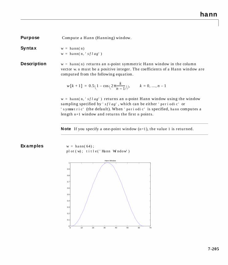
hann
7-205
7hannPurpose Compute a Hann (Hanning) window.
Syntax w = hann(n)w = hann(n,'sflag')
Description w = hann(n) returns an n-point symmetric Hann window in the columnvector w. n must be a positive integer. The coefficients of a Hann window arecomputed from the following equation.
w = hann(n,'sflag') returns an n-point Hann window using the windowsampling specified by 'sflag', which can be either 'periodic' or'symmetric' (the default). When 'periodic' is specified, hann computes alength n+1 window and returns the first n points.
Note If you specify a one-point window (n=1), the value 1 is returned.
Examples w = hann(64);plot(w); title('Hann Window')
w k 1+[ ] 0.5 1 2π kn 1–-------------
cos–
k 0= … n 1–, , ,=
0 10 20 30 40 50 60 700
0.1
0.2
0.3
0.4
0.5
0.6
0.7
0.8
0.9
1Hann Window

hann
7-206
See Also
References [1] Oppenheim, A.V., and R.W. Schafer, Discrete-Time Signal Processing,Prentice-Hall, 1989, pp. 447-448.
bartlett Compute a Bartlett window.
blackman Compute a Blackman window.
boxcar Compute a rectangular window.
chebwin Compute a Chebyshev window.
hamming Compute a Hamming window.
kaiser Compute a Kaiser window.
triang Compute a triangular window.
hilbert
7-207
7hilbertPurpose Compute the discrete-time analytic signal using the Hilbert transform.
Syntax x = hilbert(xr)x = hilbert(xr,n)
Description x = hilbert(xr) returns a complex helical sequence, sometimes called theanalytic signal, from a real data sequence. The analytic signal x = xr + i*xihas a real part, xr, which is the original data, and an imaginary part, xi, whichcontains the Hilbert transform. The imaginary part is a version of the originalreal sequence with a 90° phase shift. Sines are therefore transformed to cosinesand vice versa. The Hilbert transformed series has the same amplitude andfrequency content as the original real data and includes phase information thatdepends on the phase of the original data.
If xr is a matrix, x = hilbert(xr) operates columnwise on the matrix, findingthe Hilbert transform of each column.
x = hilbert(xr,n) uses an n point FFT to compute the Hilbert transform.The input data xr is zero-padded or truncated to length n, as appropriate.
The Hilbert transform is useful in calculating instantaneous attributes of atime series, especially the amplitude and frequency. The instantaneousamplitude is the amplitude of the complex Hilbert transform; theinstantaneous frequency is the time rate of change of the instantaneous phaseangle. For a pure sinusoid, the instantaneous amplitude and frequency areconstant. The instantaneous phase, however, is a sawtooth, reflecting the wayin which the local phase angle varies linearly over a single cycle. For mixturesof sinusoids, the attributes are short term, or local, averages spanning no morethan two or three points.
Reference [1] describes the Kolmogorov method for minimum phasereconstruction, which involves taking the Hilbert transform of the logarithm ofthe spectral density of a time series. The toolbox function rceps performs thisreconstruction.
For a discrete-time analytic signal x, the last half of fft(x) is zero, and thefirst (DC) and center (Nyquist) elements of fft(x) are purely real.

hilbert
7-208
Algorithm The analytic signal for a sequence x has a one-sided Fourier transform, that is,negative frequencies are 0. To approximate the analytic signal, hilbertcalculates the FFT of the input sequence, replaces those FFT coefficients thatcorrespond to negative frequencies with zeros, and calculates the inverse FFTof the result.
In detail, hilbert uses a four-step algorithm:
1 It calculates the FFT of the input sequence, storing the result in a vector x.
2 It creates a vector h whose elements h(i) have the values:
- 1 for i = 1, (n/2)+1
- 2 for i = 2, 3, ... , (n/2)
- 0 for i = (n/2)+2, ... , n
3 It calculates the element-wise product of x and h.
4 It calculates the inverse FFT of the sequence obtained in step 3 and returnsthe first n elements of the result.
If the input data xr is a matrix, hilbert operates in a similar manner,extending each step above to handle the matrix case.
Example xr = [1 2 3 4];x = hilbert(xr)
x = 1.0000+1.0000i 2.0000-1.0000i 3.0000-1.0000i 4.0000+1.0000i
You can see that the imaginary part, imag(x) = [1 -1 -1 1], is the Hilberttransform of xr, and the real part, real(x) = [1 2 3 4], is simply xr itself.Note that the last half of fft(x) = [10 -4+4i -2 0] is zero (in this example,the last half is just the last element), and that the DC and Nyquist elements offft(x), 10 and -2 respectively, are purely real.
See Also fft One-dimensional fast Fourier transform.
ifft One-dimensional inverse fast Fourier transform.
rceps Real cepstrum and minimum phase reconstruction.

hilbert
7-209
References [1] Claerbout, J.F., Fundamentals of Geophysical Data Processing,McGraw-Hill, 1976, pp. 59-62.
[2] Marple, S.L., “Computing the discrete-time analytic signal via FFT,” IEEETransactions on Signal Processing, Vol. 47, No. 9 (September 1999),pp. 2600-2603.
[3] Oppenheim, A.V., and R.W. Schafer, Discrete-Time Signal Processing,2nd ed., Prentice-Hall, 1998.

icceps
7-210
7iccepsPurpose Inverse complex cepstrum.
Syntax x = icceps(xhat,nd)
Description x = icceps(xhat,nd) returns the inverse complex cepstrum of the (assumedreal) sequence xhat, removing nd samples of delay. If xhat was obtained withcceps(x), then the amount of delay that was added to x was the element ofround(unwrap(angle(fft(x)))/pi) corresponding to π radians.
See Also
References [1] Oppenheim, A.V., and R.W. Schafer, Discrete-Time Signal Processing,Prentice-Hall, 1989.
cceps Complex cepstral analysis.
hilbert Hilbert transform.
rceps Real cepstrum and minimum phase reconstruction.
unwrap Unwrap phase angles.

idct
7-211
7idctPurpose Inverse discrete cosine transform.
Syntax x = idct(y)x = idct(y,n)
Description The inverse discrete cosine transform reconstructs a sequence from its discretecosine transform (DCT) coefficients. The idct function is the inverse of the dctfunction.
x = idct(y) returns the inverse discrete cosine transform of y
where
and N = length(x), which is the same as length(y). The series is indexedfrom n = 1 and k = 1 instead of the usual n = 0 and k = 0 because MATLABvectors run from 1 to N instead of from 0 to N-1.
x = idct(y,n) appends zeros or truncates the vector y to length n beforetransforming.
If y is a matrix, idct transforms its columns.
See Also
x n( ) w k( )y k( ) π 2n 1–( ) k 1–( )2N
-------------------------------------------cos
k 1=
N
n 1 … N, ,=,=
w k( )
1N
--------- k 1=,
2N---- 2 k N≤ ≤,
=
dct Discrete cosine transform (DCT).
dct2 Two-dimensional DCT (see the Image Processing Toolboxdocumentation).
idct2 Two-dimensional inverse DCT (see the Image Processing Toolboxdocumentation).
ifft One-dimensional inverse fast Fourier transform.

idct
7-212
References [1] Jain, A.K., Fundamentals of Digital Image Processing, Prentice-Hall, 1989.
[2] Pennebaker, W.B., and J.L. Mitchell, JPEG Still Image Data CompressionStandard, Van Nostrand Reinhold, 1993, Chapter 4.
ifft
7-213
7ifftPurpose One-dimensional inverse fast Fourier transform.
Syntax y = ifft(x)y = ifft(x,n)
Description ifft computes the inverse Fourier transform of a vector or array. This functionimplements the inverse transform given by
where WN = e-j(2π/N) and N = length(x). Note that the series is indexed asn + 1 and k + 1 instead of the usual n and k because MATLAB vectors run from1 to N instead of from 0 to N-1.
y = ifft(x) is the inverse Fourier transform of vector x. If x is an array, y isthe inverse FFT of each column of the matrix.
y = ifft(x,n) is the n-point inverse FFT. If the length of x is less than n, ifftpads x with trailing zeros to length n. If the length of x is greater than n, iffttruncates the sequence x. When x is an array, ifft adjusts the length of thecolumns in the same manner.
The ifft function is part of the standard MATLAB language.
Algorithm The ifft function is an M-file. The algorithm for ifft is the same as that forfft, except for a sign change and a scale factor of n = length(x). The executiontime is fastest when n is a power of two and slowest when n is a large prime.
See Also
x n 1+( )1N---- X k 1+( )Wn
kn–
k 0=
N 1–
=
fft One-dimensional fast Fourier transform.
fft2 Two-dimensional fast Fourier transform.
fftshift Rearrange the outputs of fft and fft2.
ifft2 Two-dimensional inverse fast Fourier transform.
ifft2
7-214
7ifft2Purpose Two-dimensional inverse fast Fourier transform.
Syntax Y = ifft2(X)Y = ifft2(X,m,n)
Description Y = ifft2(X) returns the two-dimensional inverse fast Fourier transform(FFT) of the array X. If X is a vector, Y has the same orientation as X.
Y = ifft2(X,m,n) truncates or zero pads X, if necessary, to create an m-by-narray before performing the inverse FFT. The result Y is also m-by-n.
For any X, ifft2(fft2(X)) equals X to within roundoff error. If X is real,ifft2(fft2(X)) may have small imaginary parts.
The ifft2 function is part of the standard MATLAB language.
Algorithm The algorithm for ifft2 is the same as that for fft2, except for a sign changeand scale factors of [m n] = size(X). The execution time is fastest when mand n are powers of two and slowest when they are large primes.
See Also fft One-dimensional fast Fourier transform.
fft2 Two-dimensional fast Fourier transform.
fftn N-dimensional fast Fourier transform (see theMATLAB documentation).
fftshift Rearrange the outputs of fft and fft2.
ifft One-dimensional inverse fast Fourier transform.
ifftn N-dimensional inverse fast Fourier transform (seethe MATLAB documentation).
impinvar
7-215
7impinvarPurpose Impulse invariance method for analog-to-digital filter conversion.
Syntax [bz,az] = impinvar(b,a,fs)[bz,az] = impinvar(b,a)[bz,az] = impinvar(b,a,fs,tol)
Description [bz,az] = impinvar(b,a,fs) creates a digital filter with numerator anddenominator coefficients bz and az, respectively, whose impulse response isequal to the impulse response of the analog filter with coefficients b and a,scaled by 1/fs. If you leave out the argument fs, or specify fs as the emptyvector [], it takes the default value of 1 Hz.
[bz,az] = impinvar(b,a,fs,tol) uses the tolerance specified by tol todetermine whether poles are repeated. A larger tolerance increases thelikelihood that impinvar interprets closely located poles as multiplicities(repeated ones). The default is 0.001, or 0.1% of a pole’s magnitude. Note thatthe accuracy of the pole values is still limited to the accuracy obtainable by theroots function.
Examples Convert an analog lowpass filter to a digital filter using impinvar with asampling frequency of 10 Hz.
[b,a] = butter(4,0.3,'s');[bz,az] = impinvar(b,a,10)
bz =
1.0e-006 *
-0.0000 0.1324 0.5192 0.1273 0
az =
1.0000 -3.9216 5.7679 -3.7709 0.9246
impinvar
7-216
Algorithm impinvar performs the impulse-invariant method of analog-to-digital transferfunction conversion discussed in reference [1]:
1 It finds the partial fraction expansion of the system represented by b and a.
2 It replaces the poles p by the poles exp(p/fs).
3 It finds the transfer function coefficients of the system from the residuesfrom step 1 and the poles from step 2.
See Also
References [1] Parks, T.W., and C.S. Burrus, Digital Filter Design, John Wiley & Sons,1987, pp. 206-209.
bilinear Bilinear transformation method for analog-to-digitalfilter conversion.
lp2bp Transform lowpass analog filters to bandpass.
lp2bs Transform lowpass analog filters to bandstop.
lp2hp Transform lowpass analog filters to highpass.
lp2lp Change the cut-off frequency for a lowpass analogfilter.
impz
7-217
7impzPurpose Compute the impulse response of digital filters.
Syntax [h,t] = impz(b,a)[h,t] = impz(b,a,n)[h,t] = impz(b,a,n,fs)impz(b,a)impz(...)
Description [h,t] = impz(b,a) computes the impulse response of the filter withnumerator coefficients b and denominator coefficients a. impz chooses thenumber of samples and returns the response in the column vector h and sampletimes in the column vector t (where t = [0:n-1]', and n = length(t) iscomputed automatically).
[h,t] = impz(b,a,n) computes n samples of the impulse response when n isan integer (t = [0:n-1]'). If n is a vector of integers, impz computes theimpulse response at those integer locations, starting the response computationfrom 0 (and t = n or t = [0 n]). If, instead of n, you include the empty vector []for the second argument, the number of samples is computed automatically bydefault.
[h,t] = impz(b,a,n,fs) computes n samples and produces a vector t oflength n so that the samples are spaced 1/fs units apart.
impz with no output arguments plots the impulse response in the currentfigure window using stem(t,h).
impz works for both real and complex input systems.
Examples Plot the first 50 samples of the impulse response of a fourth-order lowpasselliptic filter with cutoff frequency of 0.4 times the Nyquist frequency.
[b,a] = ellip(4,0.5,20,0.4);impz(b,a,50)
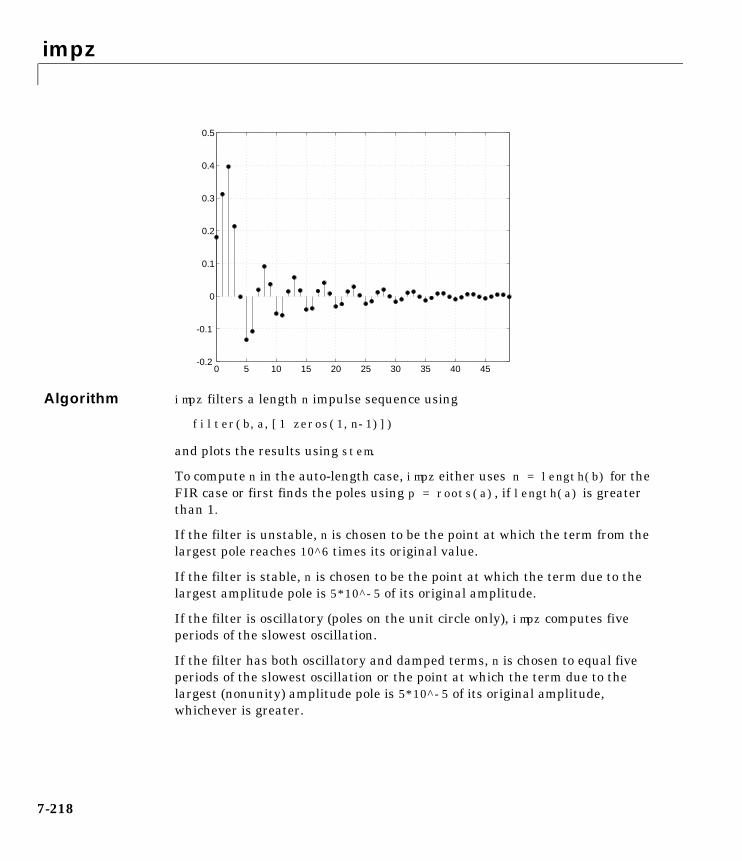
impz
7-218
Algorithm impz filters a length n impulse sequence using
filter(b,a,[1 zeros(1,n-1)])
and plots the results using stem.
To compute n in the auto-length case, impz either uses n = length(b) for theFIR case or first finds the poles using p = roots(a), if length(a) is greaterthan 1.
If the filter is unstable, n is chosen to be the point at which the term from thelargest pole reaches 10^6 times its original value.
If the filter is stable, n is chosen to be the point at which the term due to thelargest amplitude pole is 5*10^-5 of its original amplitude.
If the filter is oscillatory (poles on the unit circle only), impz computes fiveperiods of the slowest oscillation.
If the filter has both oscillatory and damped terms, n is chosen to equal fiveperiods of the slowest oscillation or the point at which the term due to thelargest (nonunity) amplitude pole is 5*10^-5 of its original amplitude,whichever is greater.
0 5 10 15 20 25 30 35 40 45-0.2
-0.1
0
0.1
0.2
0.3
0.4
0.5

impz
7-219
impz also allows for delays in the numerator polynomial. The number of delaysis incorporated into the computation for the number of samples.
See Also impulse Unit impulse response (see the Control System Toolboxdocumentation).
stem Plot discrete sequence data (see the MATLABdocumentation).
interp
7-220
7interpPurpose Increase sampling rate by an integer factor (interpolation).
Syntax y = interp(x,r)y = interp(x,r,l,alpha)[y,b] = interp(x,r,l,alpha)
Description Interpolation increases the original sampling rate for a sequence to a higherrate. interp performs lowpass interpolation by inserting zeros into the originalsequence and then applying a special lowpass filter.
y = interp(x,r) increases the sampling rate of x by a factor of r. Theinterpolated vector y is r times longer than the original input x.
y = interp(x,r,l,alpha) specifies l (filter length) and alpha (cut-offfrequency). The default value for l is 4 and the default value for alpha is 0.5.
[y,b] = interp(x,r,l,alpha) returns vector b containing the filtercoefficients used for the interpolation.
Examples Interpolate a signal by a factor of four.
t = 0:0.001:1; % Time vectorx = sin(2*pi*30*t) + sin(2*pi*60*t);y = interp(x,4);stem(x(1:30)); title('Original Signal');figurestem(y(1:120)); title('Interpolated Signal');
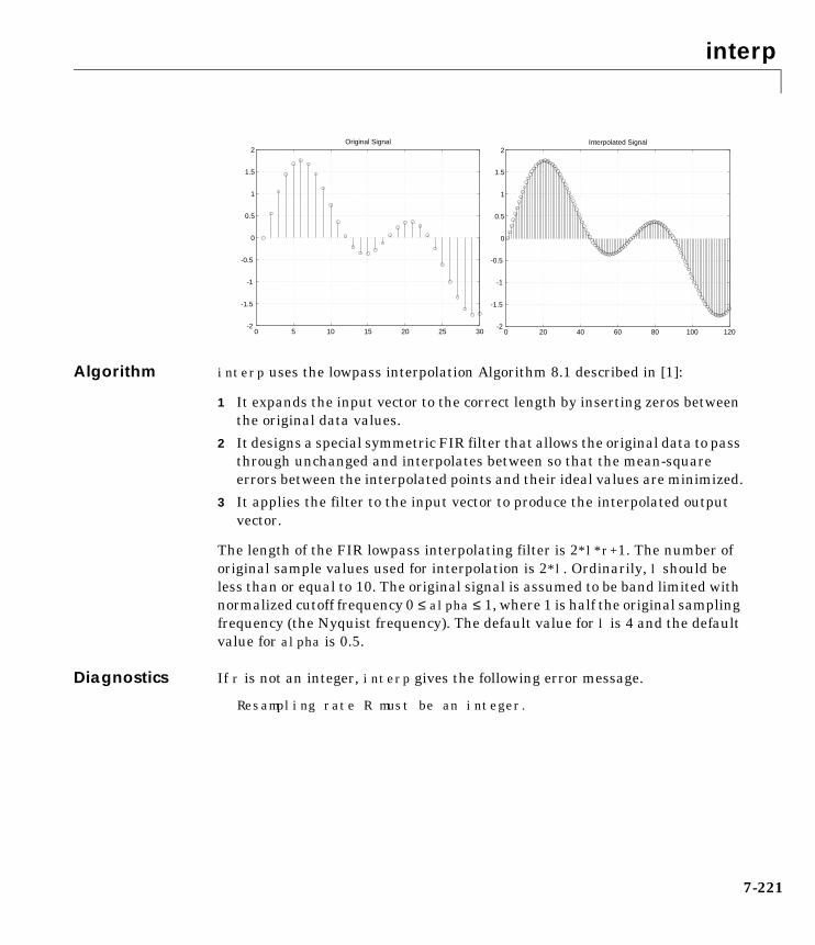
interp
7-221
Algorithm interp uses the lowpass interpolation Algorithm 8.1 described in [1]:
1 It expands the input vector to the correct length by inserting zeros betweenthe original data values.
2 It designs a special symmetric FIR filter that allows the original data to passthrough unchanged and interpolates between so that the mean-squareerrors between the interpolated points and their ideal values are minimized.
3 It applies the filter to the input vector to produce the interpolated outputvector.
The length of the FIR lowpass interpolating filter is 2*l*r+1. The number oforiginal sample values used for interpolation is 2*l. Ordinarily, l should beless than or equal to 10. The original signal is assumed to be band limited withnormalized cutoff frequency 0 ≤ alpha ≤ 1, where 1 is half the original samplingfrequency (the Nyquist frequency). The default value for l is 4 and the defaultvalue for alpha is 0.5.
Diagnostics If r is not an integer, interp gives the following error message.
Resampling rate R must be an integer.
0 20 40 60 80 100 120-2
-1.5
-1
-0.5
0
0.5
1
1.5
2Interpolated Signal
0 5 10 15 20 25 30-2
-1.5
-1
-0.5
0
0.5
1
1.5
2Original Signal
interp
7-222
See Also
References [1] Programs for Digital Signal Processing, IEEE Press, New York, 1979,Algorithm 8.1.
decimate Decrease the sampling rate for a sequence(decimation).
interp1 One-dimensional data interpolation (table lookup)(see the MATLAB documentation).
resample Change sampling rate by any rational factor.
spline Cubic spline interpolation (see the MATLABdocumentation).
upfirdn Upsample, apply an FIR filter, and downsample.
intfilt
7-223
7intfiltPurpose Interpolation FIR filter design.
Syntax b = intfilt(r,l,alpha)b = intfilt(r,n,'Lagrange')
Description b = intfilt(r,l,alpha) designs a linear phase FIR filter that performs idealbandlimited interpolation using the nearest 2*l nonzero samples, when usedon a sequence interleaved with r-1 consecutive zeros every r samples. Itassumes an original bandlimitedness of alpha times the Nyquist frequency.The returned filter is identical to that used by interp.
b = intfilt(r,n,'Lagrange') or
b = intfilt(r,n,'l') designs an FIR filter that performs nth-orderLagrange polynomial interpolation on a sequence interleaved with r-1consecutive zeros every r samples. b has length (n + 1)*r for n even, and length(n + 1)*r-1 for n odd.
Both types of filters are basically lowpass and are intended for interpolationand decimation.
Examples Design a digital interpolation filter to upsample a signal by four, using thebandlimited method.
alpha = 0.5; % "Bandlimitedness" factorh1 = intfilt(4,2,alpha); % Bandlimited interpolation
The filter h1 works best when the original signal is bandlimited to alpha timesthe Nyquist frequency. Create a bandlimited noise signal.
randn('state',0)x = filter(fir1(40,0.5),1,randn(200,1)); % Bandlimit
Now zero pad the signal with three zeros between every sample. The resultingsequence is four times the length of x.
xr = reshape([x zeros(length(x),3)]',4*length(x),1);
Interpolate using the filter command.
y = filter(h1,1,xr);
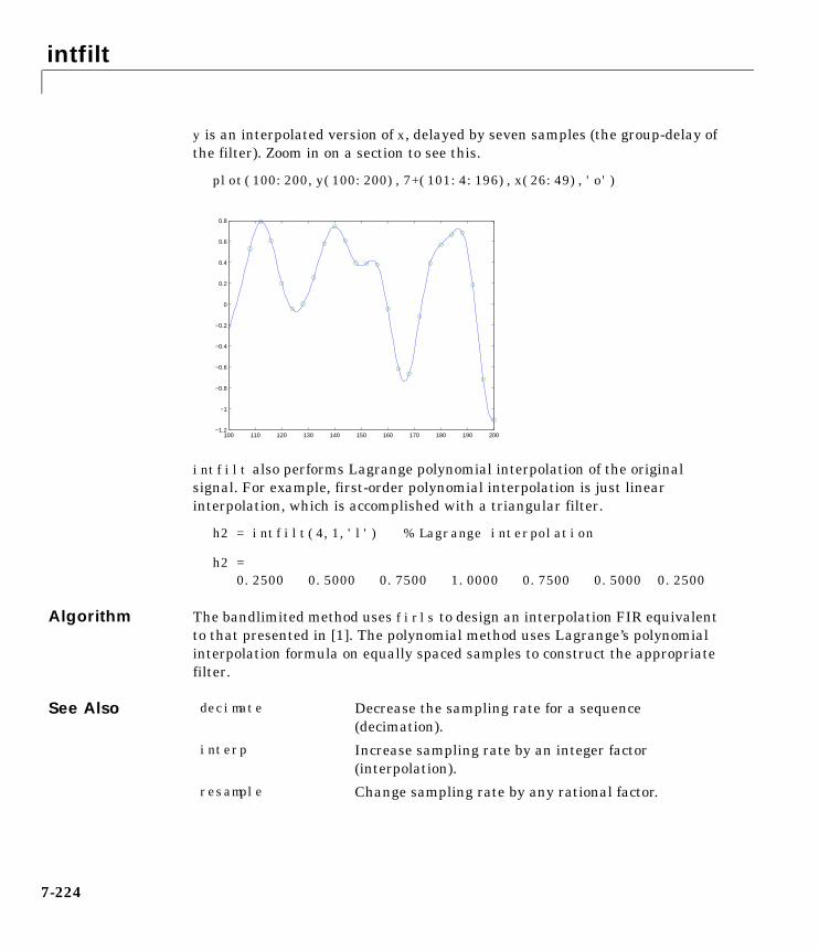
intfilt
7-224
y is an interpolated version of x, delayed by seven samples (the group-delay ofthe filter). Zoom in on a section to see this.
plot(100:200,y(100:200),7+(101:4:196),x(26:49),'o')
intfilt also performs Lagrange polynomial interpolation of the originalsignal. For example, first-order polynomial interpolation is just linearinterpolation, which is accomplished with a triangular filter.
h2 = intfilt(4,1,'l') % Lagrange interpolation
h2 = 0.2500 0.5000 0.7500 1.0000 0.7500 0.5000 0.2500
Algorithm The bandlimited method uses firls to design an interpolation FIR equivalentto that presented in [1]. The polynomial method uses Lagrange’s polynomialinterpolation formula on equally spaced samples to construct the appropriatefilter.
See Also
100 110 120 130 140 150 160 170 180 190 200−1.2
−1
−0.8
−0.6
−0.4
−0.2
0
0.2
0.4
0.6
0.8
decimate Decrease the sampling rate for a sequence(decimation).
interp Increase sampling rate by an integer factor(interpolation).
resample Change sampling rate by any rational factor.

intfilt
7-225
References [1] Oetken, Parks, and Schüßler, “New Results in the Design of DigitalInterpolators,” IEEE Trans. Acoust., Speech, Signal Processing, Vol. ASSP-23(June 1975), pp. 301-309.

invfreqs
7-226
7invfreqsPurpose Identify continuous-time filter parameters from frequency response data.
Syntax [b,a] = invfreqs(h,w,nb,na)[b,a] = invfreqs(h,w,nb,na,wt)[b,a] = invfreqs(h,w,nb,na,wt,iter)[b,a] = invfreqs(h,w,nb,na,wt,iter,tol)[b,a] = invfreqs(h,w,nb,na,wt,iter,tol,'trace')[b,a] = invfreqs(h,w,'complex',nb,na,...)
Description invfreqs is the inverse operation of freqs; it finds a continuous-time transferfunction that corresponds to a given complex frequency response. From alaboratory analysis standpoint, invfreqs is useful in converting magnitudeand phase data into transfer functions.
[b,a] = invfreqs(h,w,nb,na) returns the real numerator and denominatorcoefficient vectors b and a of the transfer function
whose complex frequency response is given in vector h at the frequency pointsspecified in vector w. Scalars nb and na specify the desired orders of thenumerator and denominator polynomials.
Frequency is specified in radians between 0 and π, and the length of h must bethe same as the length of w. invfreqs uses conj(h) at -w to ensure the properfrequency domain symmetry for a real filter.
[b,a] = invfreqs(h,w,nb,na,wt) weights the fit-errors versus frequency,where wt is a vector of weighting factors the same length as w.
[b,a] = invfreqs(h,w,nb,na,wt,iter) and
[b,a] = invfreqs(h,w,nb,na,wt,iter,tol) provide a superior algorithmthat guarantees stability of the resulting linear system and searches for thebest fit using a numerical, iterative scheme. The iter parameter tellsinvfreqs to end the iteration when the solution has converged, or after iteriterations, whichever comes first. invfreqs defines convergence as occurringwhen the norm of the (modified) gradient vector is less than tol, where tol is
H s( )B s( )A s( )----------- b 1( )snb b 2( )snb 1– b nb 1+( )+ + +
a 1( )sna a 2( )sna 1– a na 1+( )+ + +-------------------------------------------------------------------------------------------------= =
invfreqs
7-227
an optional parameter that defaults to 0.01. To obtain a weight vector of allones, use
invfreqs(h,w,nb,na,[],iter,tol)
[b,a] = invfreqs(h,w,nb,na,wt,iter,tol,'trace') displays a textualprogress report of the iteration.
[b,a] = invfreqs(h,w,'complex',nb,na,...) creates a complex filter. Inthis case no symmetry is enforced, and the frequency is specified in radiansbetween -π and π.
Remarks When building higher order models using high frequencies, it is important toscale the frequencies, dividing by a factor such as half the highest frequencypresent in w, so as to obtain well conditioned values of a and b. This correspondsto a rescaling of time.
Examples Example 1Convert a simple transfer function to frequency response data and then backto the original filter coefficients.
a = [1 2 3 2 1 4]; b = [1 2 3 2 3];[h,w] = freqs(b,a,64);[bb,aa] = invfreqs(h,w,4,5)
bb =
1.0000 2.0000 3.0000 2.0000 3.0000
aa =
1.0000 2.0000 3.0000 2.0000 1.0000 4.0000
invfreqs
7-228
Notice that bb and aa are equivalent to b and a, respectively. However, aa haspoles in the left half-plane and thus the system is unstable. Use invfreqs’siterative algorithm to find a stable approximation to the system.
[bbb,aaa] = invfreqs(h,w,4,5,[],30)
bbb =
0.6816 2.1015 2.6694 0.9113 -0.1218
aaa =
1.0000 3.4676 7.4060 6.2102 2.5413 0.0001
Example 2Suppose you have two vectors, mag and phase, that contain magnitude andphase data gathered in a laboratory, and a third vector w of frequencies. Youcan convert the data into a continuous-time transfer function using invfreqs.
[b,a] = invfreqs(mag.*exp(j*phase),w,2,3);
Algorithm By default, invfreqs uses an equation error method to identify the best modelfrom the data. This finds b and a in
by creating a system of linear equations and solving them with MATLAB’s \operator. Here A(w(k)) and B(w(k)) are the Fourier transforms of thepolynomials a and b, respectively, at the frequency w(k), and n is the numberof frequency points (the length of h and w). This algorithm is based on Levi [1].Several variants have been suggested in the literature, where the weightingfunction wt gives less attention to high frequencies.
minb a,
wt k( ) h k( )A w k( )( ) B w k( )( )– 2
k 1=
n
invfreqs
7-229
The superior (“output-error”) algorithm uses the damped Gauss-Newton methodfor iterative search [2], with the output of the first algorithm as the initialestimate. This solves the direct problem of minimizing the weighted sum of thesquared error between the actual and the desired frequency response points.
See Also
References [1] Levi, E.C., “Complex-Curve Fitting,” IRE Trans. on Automatic Control,Vol. AC-4 (1959), pp. 37-44.
[2] Dennis, J.E., Jr., and R.B. Schnabel. Numerical Methods for UnconstrainedOptimization and Nonlinear Equations. Englewood Cliffs, NJ: Prentice-Hall,1983.
minb a,
wt k( ) h k( )B w k( )( )A w k( )( )--------------------–
2
k 1=
n
freqs Compute the frequency response of analog filters.
freqz Compute the frequency response of digital filters.
invfreqz Identify a discrete-time filter from frequency data.
prony Implement Prony’s method for time domain IIR filterdesign.

invfreqz
7-230
7invfreqzPurpose Identify discrete-time filter parameters from frequency response data.
Syntax [b,a] = invfreqz(h,w,nb,na)[b,a] = invfreqz(h,w,nb,na,wt)[b,a] = invfreqz(h,w,nb,na,wt,iter)[b,a] = invfreqz(h,w,nb,na,wt,iter,tol)[b,a] = invfreqz(h,w,nb,na,wt,iter,tol,'trace')[b,a] = invfreqz(h,w,'complex',nb,na,...)
Description invfreqz is the inverse operation of freqz; it finds a discrete-time transferfunction that corresponds to a given complex frequency response. From alaboratory analysis standpoint, invfreqz can be used to convert magnitudeand phase data into transfer functions.
[b,a] = invfreqz(h,w,nb,na) returns the real numerator and denominatorcoefficients in vectors b and a of the transfer function
whose complex frequency response is given in vector h at the frequency pointsspecified in vector w. Scalars nb and na specify the desired orders of thenumerator and denominator polynomials.
Frequency is specified in radians between 0 and π, and the length of h must bethe same as the length of w. invfreqz uses conj(h) at -w to ensure the properfrequency domain symmetry for a real filter.
[b,a] = invfreqz(h,w,nb,na,wt) weights the fit-errors versus frequency,where wt is a vector of weighting factors the same length as w.
[b,a] = invfreqz(h,w,nb,na,wt,iter) and
[b,a] = invfreqz(h,w,nb,na,wt,iter,tol) provide a superior algorithmthat guarantees stability of the resulting linear system and searches for thebest fit using a numerical, iterative scheme. The iter parameter tellsinvfreqz to end the iteration when the solution has converged, or after iteriterations, whichever comes first. invfreqz defines convergence as occurringwhen the norm of the (modified) gradient vector is less than tol, where tol is
H z( )B z( )A z( )----------- b 1( ) b 2( )z 1– b nb 1+( )z nb–+ + +
a 1( ) a 2( )z 1– a na 1+( )z na–+ + +--------------------------------------------------------------------------------------------= =
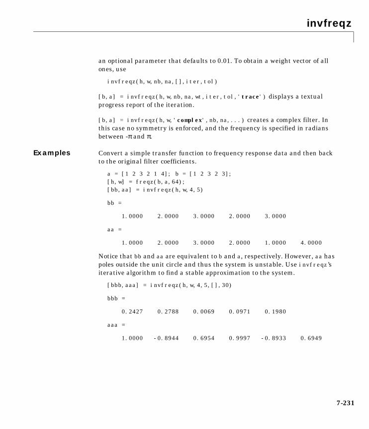
invfreqz
7-231
an optional parameter that defaults to 0.01. To obtain a weight vector of allones, use
invfreqz(h,w,nb,na,[],iter,tol)
[b,a] = invfreqz(h,w,nb,na,wt,iter,tol,'trace') displays a textualprogress report of the iteration.
[b,a] = invfreqz(h,w,'complex',nb,na,...) creates a complex filter. Inthis case no symmetry is enforced, and the frequency is specified in radiansbetween -π and π.
Examples Convert a simple transfer function to frequency response data and then backto the original filter coefficients.
a = [1 2 3 2 1 4]; b = [1 2 3 2 3];[h,w] = freqz(b,a,64);[bb,aa] = invfreqz(h,w,4,5)
bb =
1.0000 2.0000 3.0000 2.0000 3.0000
aa =
1.0000 2.0000 3.0000 2.0000 1.0000 4.0000
Notice that bb and aa are equivalent to b and a, respectively. However, aa haspoles outside the unit circle and thus the system is unstable. Use invfreqz’siterative algorithm to find a stable approximation to the system.
[bbb,aaa] = invfreqz(h,w,4,5,[],30)
bbb =
0.2427 0.2788 0.0069 0.0971 0.1980
aaa =
1.0000 -0.8944 0.6954 0.9997 -0.8933 0.6949
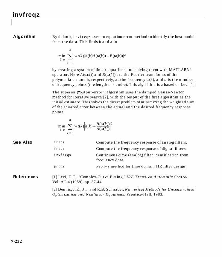
invfreqz
7-232
Algorithm By default, invfreqz uses an equation error method to identify the best modelfrom the data. This finds b and a in
by creating a system of linear equations and solving them with MATLAB’s \operator. Here A(ω(k)) and B(ω(k)) are the Fourier transforms of thepolynomials a and b, respectively, at the frequency ω(k), and n is the numberof frequency points (the length of h and w). This algorithm is a based on Levi [1].
The superior (“output-error”) algorithm uses the damped Gauss-Newtonmethod for iterative search [2], with the output of the first algorithm as theinitial estimate. This solves the direct problem of minimizing the weighted sumof the squared error between the actual and the desired frequency responsepoints.
See Also
References [1] Levi, E.C., “Complex-Curve Fitting,” IRE Trans. on Automatic Control,Vol. AC-4 (1959), pp. 37-44.
[2] Dennis, J.E., Jr., and R.B. Schnabel, Numerical Methods for UnconstrainedOptimization and Nonlinear Equations, Prentice-Hall, 1983.
minb a,
wt k( ) h k( )A ω k( )( ) B ω k( )( )– 2
k 1=
n
minb a,
wt k( ) h k( )B ω k( )( )A ω k( )( )-------------------–
2
k 1=
n
freqs Compute the frequency response of analog filters.
freqz Compute the frequency response of digital filters.
invfreqs Continuous-time (analog) filter identification fromfrequency data.
prony Prony’s method for time domain IIR filter design.
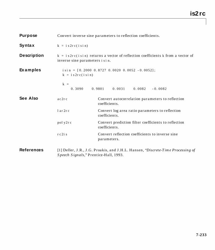
is2rc
7-233
7is2rcPurpose Convert inverse sine parameters to reflection coefficients.
Syntax k = is2rc(isin)
Description k = is2rc(isin) returns a vector of reflection coefficients k from a vector ofinverse sine parameters isin.
Examples isin = [0.2000 0.8727 0.0020 0.0052 -0.0052];k = is2rc(isin)
k = 0.3090 0.9801 0.0031 0.0082 -0.0082
See Also
References [1] Deller, J.R., J.G. Proakis, and J.H.L. Hansen, “Discrete-Time Processing ofSpeech Signals,” Prentice-Hall, 1993.
ac2rc Convert autocorrelation parameters to reflectioncoefficients.
lar2rc Convert log area ratio parameters to reflectioncoefficients.
poly2rc Convert prediction filter coefficients to reflectioncoefficients.
rc2is Convert reflection coefficients to inverse sineparameters.
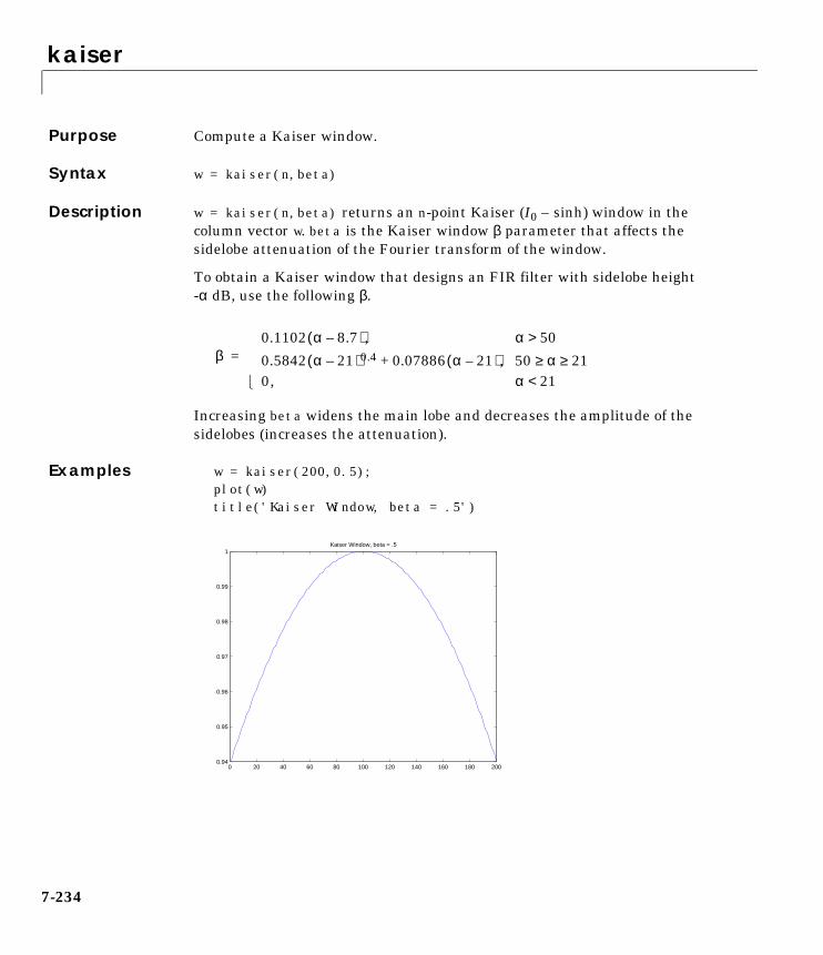
kaiser
7-234
7kaiserPurpose Compute a Kaiser window.
Syntax w = kaiser(n,beta)
Description w = kaiser(n,beta) returns an n-point Kaiser (I0 – sinh) window in thecolumn vector w. beta is the Kaiser window β parameter that affects thesidelobe attenuation of the Fourier transform of the window.
To obtain a Kaiser window that designs an FIR filter with sidelobe height-α dB, use the following β.
Increasing beta widens the main lobe and decreases the amplitude of thesidelobes (increases the attenuation).
Examples w = kaiser(200,0.5);plot(w)title('Kaiser Window, beta = .5')
β0.1102 α 8.7–( ), α 50>0.5842 α 21–( )0.4 0.07886 α 21–( )+ , 50 α 21≥ ≥0, α 21<
=
0 20 40 60 80 100 120 140 160 180 2000.94
0.95
0.96
0.97
0.98
0.99
1Kaiser Window, beta = .5
kaiser
7-235
See Also
References [1] Kaiser, J.F., “Nonrecursive Digital Filter Design Using the - sinhWindow Function,” Proc. 1974 IEEE Symp. Circuits and Systems, (April 1974),pp. 20-23.
[2] Selected Papers in Digital Signal Processing II, IEEE Press, New York,1975.
[3] Oppenheim, A.V., and R.W. Schafer, Discrete-Time Signal Processing,Prentice-Hall, 1989, p. 453.
bartlett Compute a Bartlett window.
blackman Compute a Blackman window.
boxcar Compute a rectangular window.
chebwin Compute a Chebyshev window.
hamming Compute a Hamming window.
hann Compute a Hann window.
kaiserord Estimate parameters for fir1 with a Kaiser window.
triang Compute a triangular window.
I0
kaiserord
7-236
7kaiserordPurpose Estimate parameters for an FIR filter design with a Kaiser window.
Syntax [n,Wn,beta,ftype] = kaiserord(f,a,dev)[n,Wn,beta,ftype] = kaiserord(f,a,dev,fs)c = kaiserord(f,a,dev,fs,'cell')
Description kaiserord returns a filter order n and beta parameter to specify a Kaiserwindow for use with the fir1 function. Given a set of specifications in thefrequency domain, kaiserord estimates the minimum FIR filter order that willapproximately meet the specifications. kaiserord converts the given filterspecifications into passband and stopband ripples and converts cutofffrequencies into the form needed for windowed FIR filter design.
[n,Wn,beta,ftype] = kaiserord(f,a,dev) finds the approximate order n,normalized frequency band edges Wn, and weights that meet inputspecifications f, a, and dev. f is a vector of band edges and a is a vectorspecifying the desired amplitude on the bands defined by f. The length of f istwice the length of a, minus 2. Together, f and a define a desired piecewiseconstant response function. dev is a vector the same size as a that specifies themaximum allowable error or deviation between the frequency response of theoutput filter and its desired amplitude, for each band. The entries in devspecify the passband ripple and the stopband attenuation. You specify eachentry in dev as a positive number, representing absolute filter gain (not indecibels).
Note If, in the vector dev, you specify unequal deviations across bands, theminimum specified deviation is used, since the Kaiser window method isconstrained to produce filters with minimum deviation in all of the bands.
fir1 can use the resulting order n, frequency vector Wn, multiband magnitudetype ftype, and the Kaiser window parameter beta. The ftype string isintended for use with fir1; it is equal to 'high' for a highpass filter and 'stop'for a bandstop filter. For multiband filters, it can be equal to 'dc-0' when thefirst band is a stopband (starting at f = 0) or 'dc-1' when the first band is apassband.
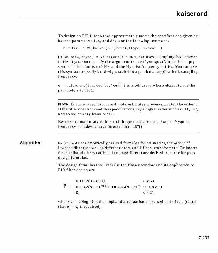
kaiserord
7-237
To design an FIR filter b that approximately meets the specifications given bykaiser parameters f, a, and dev, use the following command.
b = fir1(n,Wn,kaiser(n+1,beta),ftype,'noscale')
[n,Wn,beta,ftype] = kaiserord(f,a,dev,fs) uses a sampling frequency fsin Hz. If you don’t specify the argument fs, or if you specify it as the emptyvector [], it defaults to 2 Hz, and the Nyquist frequency is 1 Hz. You can usethis syntax to specify band edges scaled to a particular application’s samplingfrequency.
c = kaiserord(f,a,dev,fs,'cell') is a cell-array whose elements are theparameters to fir1.
Note In some cases, kaiserord underestimates or overestimates the order n.If the filter does not meet the specifications, try a higher order such as n+1, n+2,and so on, or a try lower order.
Results are inaccurate if the cutoff frequencies are near 0 or the Nyquistfrequency, or if dev is large (greater than 10%).
Algorithm kaiserord uses empirically derived formulas for estimating the orders oflowpass filters, as well as differentiators and Hilbert transformers. Estimatesfor multiband filters (such as bandpass filters) are derived from the lowpassdesign formulas.
The design formulas that underlie the Kaiser window and its application toFIR filter design are
where α = -20log10δ is the stopband attenuation expressed in decibels (recallthat δp = δs is required).
β0.1102 α 8.7–( ), α 50>0.5842 α 21–( )0.4 0.07886 α 21–( )+ , 50 α 21≥ ≥0, α 21<
=

kaiserord
7-238
The design formula is
where n is the filter order and ∆ω is the width of the smallest transition region.
Examples Example 1Design a lowpass filter with passband defined from 0 to 1 kHz and stopbanddefined from 1500 Hz to 4 kHz. Specify a passband ripple of 5% and a stopbandattenuation of 40 dB.
fsamp = 8000;fcuts = [1000 1500];mags = [1 0];devs = [0.05 0.01];[n,Wn,beta,ftype] = kaiserord(fcuts,mags,devs,fsamp);hh = fir1(n,Wn,ftype,kaiser(n+1,beta),'noscale');freqz(hh)
n α 7.95–2.285 ω∆( )----------------------------=
0 0.1 0.2 0.3 0.4 0.5 0.6 0.7 0.8 0.9 1−1400
−1200
−1000
−800
−600
−400
−200
0
Normalized Frequency (×π rad/sample)
Pha
se (
degr
ees)
0 0.1 0.2 0.3 0.4 0.5 0.6 0.7 0.8 0.9 1−120
−100
−80
−60
−40
−20
0
20
Normalized Frequency (×π rad/sample)
Mag
nitu
de (
dB)
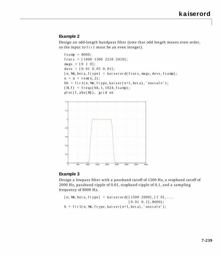
kaiserord
7-239
Example 2Design an odd-length bandpass filter (note that odd length means even order,so the input to fir1 must be an even integer).
fsamp = 8000;fcuts = [1000 1300 2210 2410];mags = [0 1 0];devs = [0.01 0.05 0.01];[n,Wn,beta,ftype] = kaiserord(fcuts,mags,devs,fsamp);n = n + rem(n,2);hh = fir1(n,Wn,ftype,kaiser(n+1,beta),'noscale');[H,f] = freqz(hh,1,1024,fsamp);plot(f,abs(H)), grid on
Example 3Design a lowpass filter with a passband cutoff of 1500 Hz, a stopband cutoff of2000 Hz, passband ripple of 0.01, stopband ripple of 0.1, and a samplingfrequency of 8000 Hz.
[n,Wn,beta,ftype] = kaiserord([1500 2000],[1 0],...[0.01 0.1],8000);
b = fir1(n,Wn,ftype,kaiser(n+1,beta),'noscale');
0 500 1000 1500 2000 2500 3000 3500 40000
0.2
0.4
0.6
0.8
1
1.2
1.4

kaiserord
7-240
This is equivalent to
c = kaiserord([1500 2000],[1 0],[0.01 0.1],8000,'cell');b = fir1(c:);
Remarks Be careful to distinguish between the meanings of filter length and filter order.The filter length is the number of impulse response samples in the FIR filter.Generally, the impulse response is indexed from n = 0 to n = L-1, where L is thefilter length. The filter order is the highest power in a z-transformrepresentation of the filter. For an FIR transfer function, this representation isa polynomial in z, where the highest power is zL-1 and the lowest power is z0.The filter order is one less than the length (L-1) and is also equal to the numberof zeros of the z polynomial.
See Also
References [1] Kaiser, J.F., “Nonrecursive Digital Filter Design Using the - sinhWindow Function,” Proc. 1974 IEEE Symp. Circuits and Systems, (April 1974),pp. 20-23.
[2] Selected Papers in Digital Signal Processing II, IEEE Press, New York,1975, pp. 123-126.
[3] Oppenheim, A.V., and R.W. Schafer, Discrete-Time Signal Processing,Prentice-Hall, 1989, pp. 458-562.
fir1 Window-based finite impulse response filter design –standard response.
kaiser Kaiser window.
remezord Parks-McClellan optimal FIR filter order estimation.
I0

lar2rc
7-241
7lar2rcPurpose Convert log area ratio parameters to reflection coefficients.
Syntax k = lar2rc(g)
Description k = lar2rc(g) returns a vector of reflection coefficients k from a vector of logarea ratio parameters g.
Examples g = [0.6389 4.5989 0.0063 0.0163 -0.0163];k = lar2rc(g)
k = 0.3090 0.9801 0.0031 0.0081 -0.0081
See Also
References [1] Deller, J.R., J.G. Proakis, and J.H.L. Hansen, “Discrete-Time Processing ofSpeech Signals,” Prentice-Hall, 1993.
ac2rc Convert autocorrelation parameters to reflectioncoefficients.
is2rc Convert inverse sine parameters to reflectioncoefficients.
poly2rc Convert prediction filter coefficients to reflectioncoefficients.
rc2lar Convert reflection coefficients to log area ratioparameters.

latc2tf
7-242
7latc2tfPurpose Convert lattice filter parameters to transfer function form.
Syntax [num,den] = latc2tf(k,v)[num,den] = latc2tf(k,'iiroption')num = latc2tf(k,'firoption')num = latc2tf(k)
Description [num,den] = latc2tf(k,v) finds the transfer function numerator num anddenominator den from the IIR lattice coefficients k and ladder coefficients v.
[num,den] = latc2tf(k,'iiroption') produces an IIR filter transferfunction according to the value of the string 'iiroption':
• 'allpole': Produces an all-pole filter transfer function from the associatedall-pole IIR lattice filter coefficients k.
• 'allpass': Produces an allpass filter transfer function from the associatedallpass IIR lattice filter coefficients k.
num = latc2tf(k,'firoption') produces an FIR filter according to the valueof the string 'firoption':
• 'min': Produces a minimum-phase FIR filter numerator from the associatedminimum-phase FIR lattice filter coefficients k.
• 'max': Produces a maximum-phase FIR filter numerator from the associatedmaximum-phase FIR lattice filter coefficients k.
• 'FIR': Produces a general FIR filter numerator from the lattice filtercoefficients k (default, if you leave off the string altogether).
See Also latcfilt Lattice and lattice-ladder filter implementation.
tf2latc Convert transfer function filter parameters to latticefilter form.
latcfilt
7-243
7latcfiltPurpose Lattice and lattice-ladder filter implementation.
Syntax [f,g] = latcfilt(k,x)[f,g] = latcfilt(k,v,x)[f,g] = latcfilt(k,1,x)[f,g,zf] = latcfilt(...,'ic',zi)
Description When filtering data, lattice coefficients can be used to represent:
• FIR filters
• All-pole IIR filters
• Allpass IIR filters
• General IIR filters
[f,g] = latcfilt(k,x) filters x with the FIR lattice coefficients in thevector k. f is the forward lattice filter result and g is the backward filter result.If , f corresponds to the minimum-phase output, and g corresponds to themaximum-phase output.
If k and x are vectors, the result is a (signal) vector. Matrix arguments arepermitted under the following rules:
• If x is a matrix and k is a vector, each column of x is processed through thelattice filter specified by k.
• If x is a vector and k is a matrix, each column of k is used to filter x, and asignal matrix is returned.
• If x and k are both matrices with the same number of columns, then the ithcolumn of k is used to filter the ith column of x. A signal matrix is returned.
[f,g] = latcfilt(k,v,x) filters x with the IIR lattice coefficients k andladder coefficients v. k and v must be vectors, while x can be a signal matrix.
[f,g] = latcfilt(k,1,x) filters x with the IIR lattice specified by k, where kand x can be vectors or matrices. f is the all-pole lattice filter result and g is theallpass filter result.
[f,g,zf] = latcfilt(...,'ic',zi) accepts a length-k vector zi specifyingthe initial condition of the lattice states. Output zf is a length-k vectorspecifying the final condition of the lattice states.
k 1≤

latcfilt
7-244
See Also filter Filter data with a recursive (IIR) or nonrecursive(FIR) filter.
latc2tf Convert lattice filter parameters to transfer functionform.
tf2latc Convert transfer function filter parameters to latticefilter form.

levinson
7-245
7levinsonPurpose Compute the Levinson-Durbin recursion.
Syntax a = levinson(r,p)
Description The Levinson-Durbin recursion is an algorithm for finding an all-pole IIR filterwith a prescribed deterministic autocorrelation sequence. It has applications infilter design, coding, and spectral estimation. The filter that levinson producesis minimum phase.
a = levinson(r,p) finds the coefficients of an pth-order autoregressive linearprocess which has r as its autocorrelation sequence. r is a real or complexdeterministic autocorrelation sequence (a vector), and p is the order ofdenominator polynomial A(z); that is, a = [1 a(2) ... a(p+1)]. The filtercoefficients are ordered in descending powers of z.
Algorithm levinson solves the symmetric Toeplitz system of linear equations
where r = [r(1) ... r(p+1)] is the input autocorrelation vector, and r(i)*
denotes the complex conjugate of r(i). The algorithm requires O(p2) flops and isthus much more efficient than the MATLAB \ command for large p. However,the levinson function uses \ for low orders to provide the fastest possibleexecution.
H z( )1
A z( )----------- 1
1 a 2( )z 1– a p 1+( )z p–+ + +-----------------------------------------------------------------------------= =
r 1( ) r 2( )∗
r p( )∗
r 2( ) r 1( ) r p 1–( )∗
r p( ) r 2( ) r 1( )
a 2( )
a 3( )
a p 1+( )
r 2( )–
r 3( )–
r p 1+( )–
=

levinson
7-246
See Also
References [1] Ljung, L., System Identification: Theory for the User, Prentice-Hall, 1987,pp. 278-280.
lpc Compute linear prediction filter coefficients.
prony Prony’s method for time domain IIR filter design.
rlevinson Compute the reverse Levinson-Durbin recursion.
schurrc Compute reflection coefficients using Schur’salgorithm.
stmcb Compute a linear model using Steiglitz-McBrideiteration.
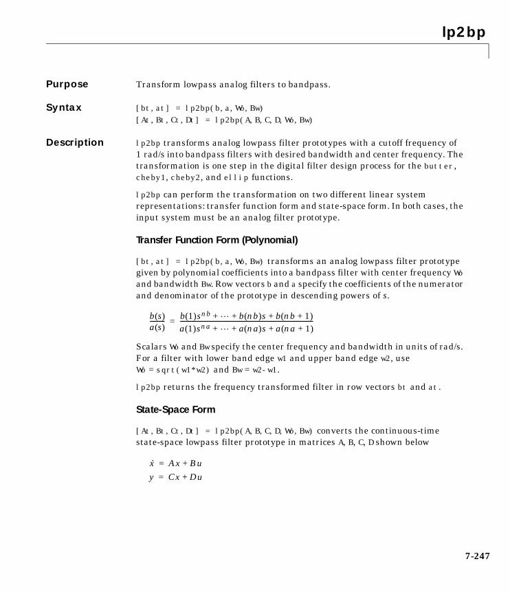
lp2bp
7-247
7lp2bpPurpose Transform lowpass analog filters to bandpass.
Syntax [bt,at] = lp2bp(b,a,Wo,Bw)[At,Bt,Ct,Dt] = lp2bp(A,B,C,D,Wo,Bw)
Description lp2bp transforms analog lowpass filter prototypes with a cutoff frequency of1 rad/s into bandpass filters with desired bandwidth and center frequency. Thetransformation is one step in the digital filter design process for the butter,cheby1, cheby2, and ellip functions.
lp2bp can perform the transformation on two different linear systemrepresentations: transfer function form and state-space form. In both cases, theinput system must be an analog filter prototype.
Transfer Function Form (Polynomial)
[bt,at] = lp2bp(b,a,Wo,Bw) transforms an analog lowpass filter prototypegiven by polynomial coefficients into a bandpass filter with center frequency Woand bandwidth Bw. Row vectors b and a specify the coefficients of the numeratorand denominator of the prototype in descending powers of s.
Scalars Wo and Bw specify the center frequency and bandwidth in units of rad/s.For a filter with lower band edge w1 and upper band edge w2, useWo = sqrt(w1*w2) and Bw = w2-w1.
lp2bp returns the frequency transformed filter in row vectors bt and at.
State-Space Form
[At,Bt,Ct,Dt] = lp2bp(A,B,C,D,Wo,Bw) converts the continuous-timestate-space lowpass filter prototype in matrices A, B, C, D shown below
b s( )a s( )---------- b 1( )snb b nb( )s b nb 1+( )+ + +
a 1( )sna a na( )s a na 1+( )+ + +---------------------------------------------------------------------------------------=
x· Ax Bu+=
y Cx Du+=

lp2bp
7-248
into a bandpass filter with center frequency Wo and bandwidth Bw. For a filterwith lower band edge w1 and upper band edge w2, use Wo = sqrt(w1*w2) andBw = w2-w1.
The bandpass filter is returned in matrices At, Bt, Ct, Dt.
Algorithm lp2bp is a highly accurate state-space formulation of the classic analog filterfrequency transformation. Consider the state-space system
where u is the input, x is the state vector, and y is the output. The Laplacetransform of the first equation (assuming zero initial conditions) is
Now if a bandpass filter is to have center frequency ω0 and bandwidth Bw, thestandard s-domain transformation is
where Q = ω0/Bw and p = s/ω0. Substituting this for s in the Laplacetransformed state-space equation, and considering the operator p as d/dtresults in
or
Now define
which, when substituted, leads to
x· Ax Bu+=
y Cx Du+=
sX s( ) AX s( ) BU s( )+=
s Q p2 1+( ) p⁄=
Qx·· Qx+ A·x Bu·+=
Qx·· A·– x B– u· Qx–=
Qω· Qx–=
Qx· Ax Qω Bu+ +=
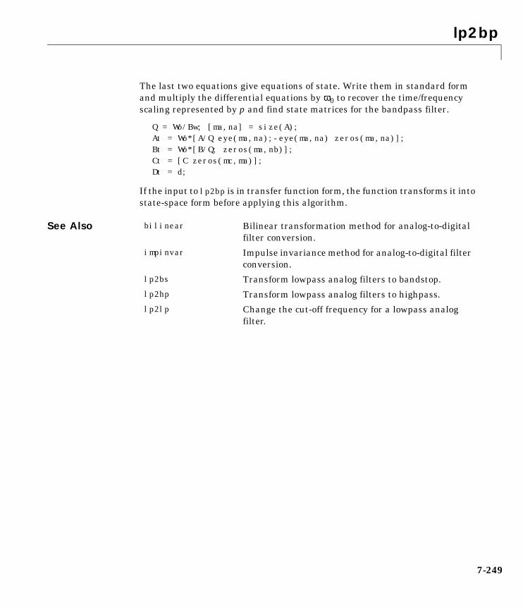
lp2bp
7-249
The last two equations give equations of state. Write them in standard formand multiply the differential equations by ω0 to recover the time/frequencyscaling represented by p and find state matrices for the bandpass filter.
Q = Wo/Bw; [ma,na] = size(A);At = Wo*[A/Q eye(ma,na);-eye(ma,na) zeros(ma,na)];Bt = Wo*[B/Q; zeros(ma,nb)];Ct = [C zeros(mc,ma)];Dt = d;
If the input to lp2bp is in transfer function form, the function transforms it intostate-space form before applying this algorithm.
See Also bilinear Bilinear transformation method for analog-to-digitalfilter conversion.
impinvar Impulse invariance method for analog-to-digital filterconversion.
lp2bs Transform lowpass analog filters to bandstop.
lp2hp Transform lowpass analog filters to highpass.
lp2lp Change the cut-off frequency for a lowpass analogfilter.
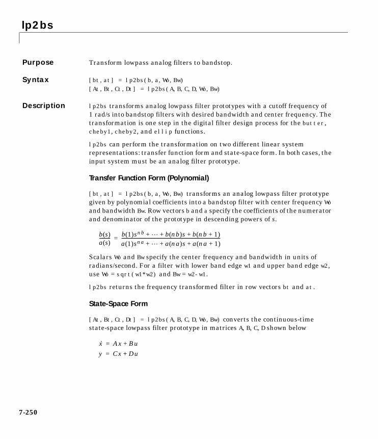
lp2bs
7-250
7lp2bsPurpose Transform lowpass analog filters to bandstop.
Syntax [bt,at] = lp2bs(b,a,Wo,Bw)[At,Bt,Ct,Dt] = lp2bs(A,B,C,D,Wo,Bw)
Description lp2bs transforms analog lowpass filter prototypes with a cutoff frequency of1 rad/s into bandstop filters with desired bandwidth and center frequency. Thetransformation is one step in the digital filter design process for the butter,cheby1, cheby2, and ellip functions.
lp2bs can perform the transformation on two different linear systemrepresentations: transfer function form and state-space form. In both cases, theinput system must be an analog filter prototype.
Transfer Function Form (Polynomial)
[bt,at] = lp2bs(b,a,Wo,Bw) transforms an analog lowpass filter prototypegiven by polynomial coefficients into a bandstop filter with center frequency Woand bandwidth Bw. Row vectors b and a specify the coefficients of the numeratorand denominator of the prototype in descending powers of s.
Scalars Wo and Bw specify the center frequency and bandwidth in units ofradians/second. For a filter with lower band edge w1 and upper band edge w2,use Wo = sqrt(w1*w2) and Bw = w2-w1.
lp2bs returns the frequency transformed filter in row vectors bt and at.
State-Space Form
[At,Bt,Ct,Dt] = lp2bs(A,B,C,D,Wo,Bw) converts the continuous-timestate-space lowpass filter prototype in matrices A, B, C, D shown below
b s( )a s( )---------- b 1( )snb b nb( )s b nb 1+( )+ + +
a 1( )sna a na( )s a na 1+( )+ + +---------------------------------------------------------------------------------------=
x· Ax Bu+=
y Cx Du+=
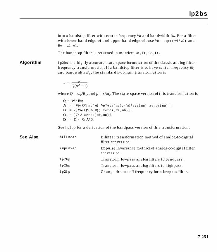
lp2bs
7-251
into a bandstop filter with center frequency Wo and bandwidth Bw. For a filterwith lower band edge w1 and upper band edge w2, use Wo = sqrt(w1*w2) andBw = w2-w1.
The bandstop filter is returned in matrices At, Bt, Ct, Dt.
Algorithm lp2bs is a highly accurate state-space formulation of the classic analog filterfrequency transformation. If a bandstop filter is to have center frequency ω0and bandwidth Bw, the standard s-domain transformation is
where Q = ω0/Bw and p = s/ω0. The state-space version of this transformation is
Q = Wo/Bw;At = [Wo/Q*inv(A) Wo*eye(ma);-Wo*eye(ma) zeros(ma)];Bt = -[Wo/Q*(A B); zeros(ma,nb)];Ct = [C/A zeros(mc,ma)];Dt = D - C/A*B;
See lp2bp for a derivation of the bandpass version of this transformation.
See Also
s pQ p2 1+( )------------------------=
bilinear Bilinear transformation method of analog-to-digitalfilter conversion.
impinvar Impulse invariance method of analog-to-digital filterconversion.
lp2bp Transform lowpass analog filters to bandpass.
lp2hp Transform lowpass analog filters to highpass.
lp2lp Change the cut-off frequency for a lowpass filter.
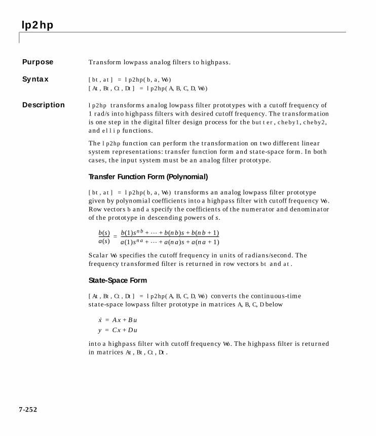
lp2hp
7-252
7lp2hpPurpose Transform lowpass analog filters to highpass.
Syntax [bt,at] = lp2hp(b,a,Wo)[At,Bt,Ct,Dt] = lp2hp(A,B,C,D,Wo)
Description lp2hp transforms analog lowpass filter prototypes with a cutoff frequency of1 rad/s into highpass filters with desired cutoff frequency. The transformationis one step in the digital filter design process for the butter, cheby1, cheby2,and ellip functions.
The lp2hp function can perform the transformation on two different linearsystem representations: transfer function form and state-space form. In bothcases, the input system must be an analog filter prototype.
Transfer Function Form (Polynomial)
[bt,at] = lp2hp(b,a,Wo) transforms an analog lowpass filter prototypegiven by polynomial coefficients into a highpass filter with cutoff frequency Wo.Row vectors b and a specify the coefficients of the numerator and denominatorof the prototype in descending powers of s.
Scalar Wo specifies the cutoff frequency in units of radians/second. Thefrequency transformed filter is returned in row vectors bt and at.
State-Space Form
[At,Bt,Ct,Dt] = lp2hp(A,B,C,D,Wo) converts the continuous-timestate-space lowpass filter prototype in matrices A, B, C, D below
into a highpass filter with cutoff frequency Wo. The highpass filter is returnedin matrices At, Bt, Ct, Dt.
b s( )a s( )---------- b 1( )snb b nb( )s b nb 1+( )+ + +
a 1( )sna a na( )s a na 1+( )+ + +---------------------------------------------------------------------------------------=
x· Ax Bu+=
y Cx Du+=

lp2hp
7-253
Algorithm lp2hp is a highly accurate state-space formulation of the classic analog filterfrequency transformation. If a highpass filter is to have cutoff frequency ω0, thestandard s-domain transformation is
The state-space version of this transformation is
At = Wo*inv(A);Bt = -Wo*(A\B);Ct = C/A;Dt = D - C/A*B;
See lp2bp for a derivation of the bandpass version of this transformation.
See Also
sω0p
-------=
bilinear Bilinear transformation method for analog-to-digitalfilter conversion.
impinvar Impulse invariance method for analog-to-digital filterconversion.
lp2bp Transform lowpass analog filters to bandpass.
lp2bs Transform lowpass analog filters to bandstop.
lp2lp Change the cut-off frequency for lowpass analogfilters.

lp2lp
7-254
7lp2lpPurpose Change the cut-off frequency for a lowpass analog filter.
Syntax [bt,at] = lp2lp(b,a,Wo)[At,Bt,Ct,Dt] = lp2lp(A,B,C,D,Wo)
Description lp2lp transforms an analog lowpass filter prototype with a cutoff frequency of1 rad/s into a lowpass filter with any specified cutoff frequency. Thetransformation is one step in the digital filter design process for the butter,cheby1, cheby2, and ellip functions.
The lp2lp function can perform the transformation on two different linearsystem representations: transfer function form and state-space form. In bothcases, the input system must be an analog filter prototype.
Transfer Function Form (Polynomial)
[bt,at] = lp2lp(b,a,Wo) transforms an analog lowpass filter prototypegiven by polynomial coefficients into a lowpass filter with cutoff frequency Wo.Row vectors b and a specify the coefficients of the numerator and denominatorof the prototype in descending powers of s.
Scalar Wo specifies the cutoff frequency in units of radians/second. lp2lpreturns the frequency transformed filter in row vectors bt and at.
State-Space Form
[At,Bt,Ct,Dt] = lp2lp(A,B,C,D,Wo) converts the continuous-timestate-space lowpass filter prototype in matrices A, B, C, D below
into a lowpass filter with cutoff frequency Wo. lp2lp returns the lowpass filterin matrices At, Bt, Ct, Dt.
b s( )a s( )---------- b 1( )snb b nb( )s b nb 1+( )+ + +
a 1( )sna a na( )s a na 1+( )+ + +---------------------------------------------------------------------------------------=
x· Ax Bu+=
y Cx Du+=
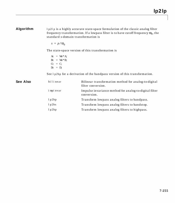
lp2lp
7-255
Algorithm lp2lp is a highly accurate state-space formulation of the classic analog filterfrequency transformation. If a lowpass filter is to have cutoff frequency ω0, thestandard s-domain transformation is
The state-space version of this transformation is
At = Wo*A;Bt = Wo*B;Ct = C;Dt = D;
See lp2bp for a derivation of the bandpass version of this transformation.
See Also
s p ω0⁄=
bilinear Bilinear transformation method for analog-to-digitalfilter conversion.
impinvar Impulse invariance method for analog-to-digital filterconversion.
lp2bp Transform lowpass analog filters to bandpass.
lp2bs Transform lowpass analog filters to bandstop.
lp2hp Transform lowpass analog filters to highpass.
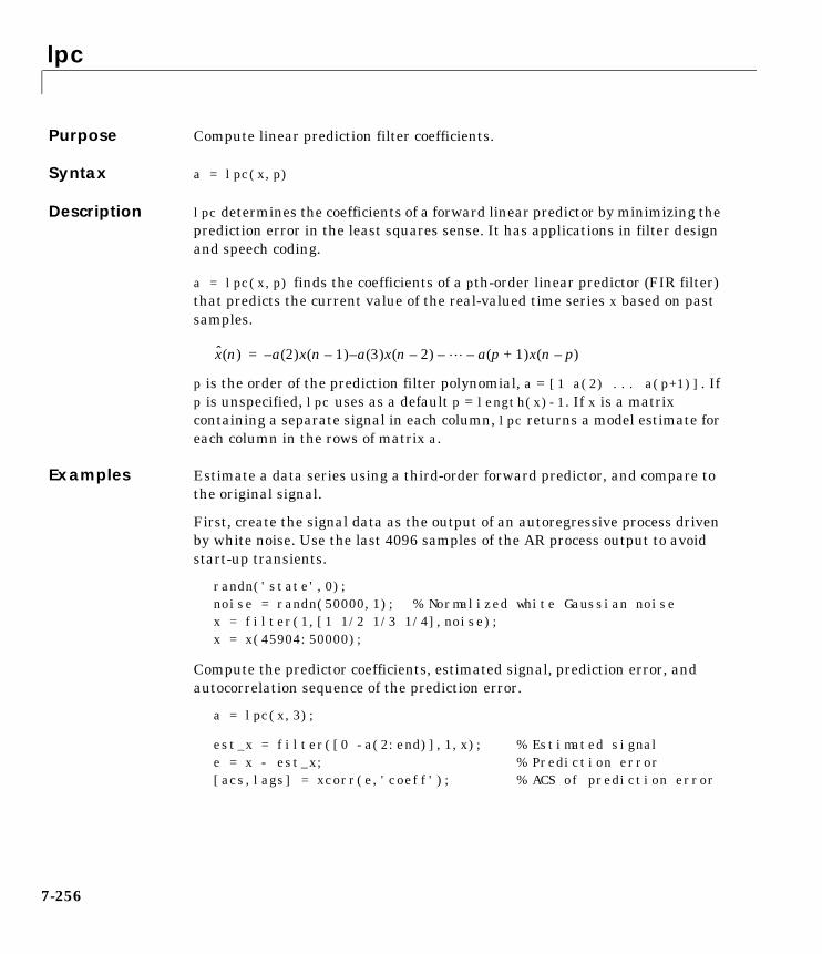
lpc
7-256
7lpcPurpose Compute linear prediction filter coefficients.
Syntax a = lpc(x,p)
Description lpc determines the coefficients of a forward linear predictor by minimizing theprediction error in the least squares sense. It has applications in filter designand speech coding.
a = lpc(x,p) finds the coefficients of a pth-order linear predictor (FIR filter)that predicts the current value of the real-valued time series x based on pastsamples.
p is the order of the prediction filter polynomial, a = [1 a(2) ... a(p+1)]. Ifp is unspecified, lpc uses as a default p = length(x)-1. If x is a matrixcontaining a separate signal in each column, lpc returns a model estimate foreach column in the rows of matrix a.
Examples Estimate a data series using a third-order forward predictor, and compare tothe original signal.
First, create the signal data as the output of an autoregressive process drivenby white noise. Use the last 4096 samples of the AR process output to avoidstart-up transients.
randn('state',0);noise = randn(50000,1); % Normalized white Gaussian noisex = filter(1,[1 1/2 1/3 1/4],noise);x = x(45904:50000);
Compute the predictor coefficients, estimated signal, prediction error, andautocorrelation sequence of the prediction error.
a = lpc(x,3);
est_x = filter([0 -a(2:end)],1,x); % Estimated signale = x - est_x; % Prediction error[acs,lags] = xcorr(e,'coeff'); % ACS of prediction error
x n( ) a– 2( )x n 1–( ) a– 3( )x n 2–( ) – a p 1+( )x n p–( )–=
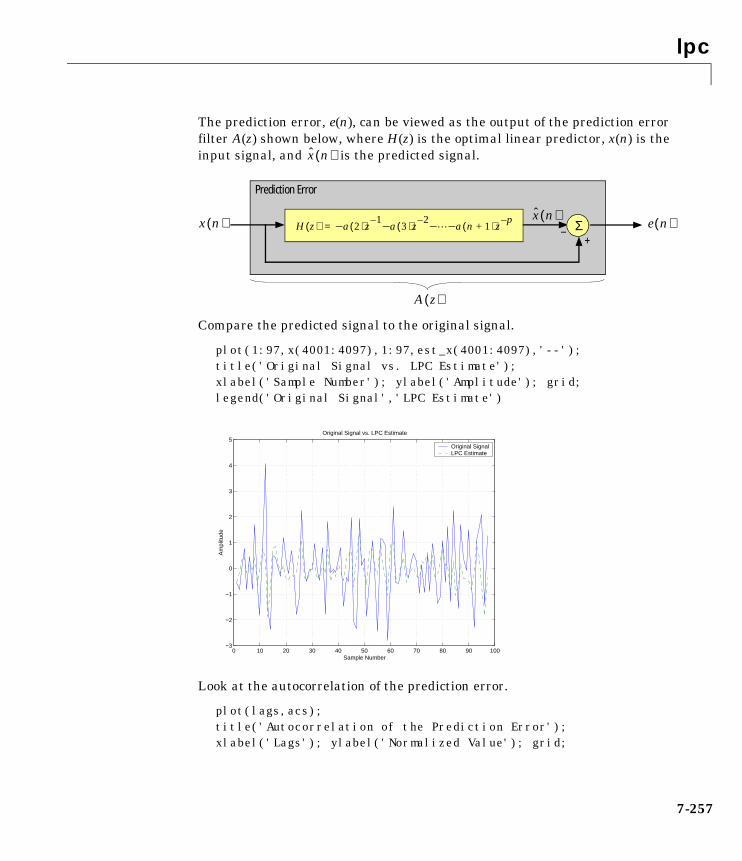
lpc
7-257
The prediction error, e(n), can be viewed as the output of the prediction errorfilter A(z) shown below, where H(z) is the optimal linear predictor, x(n) is theinput signal, and is the predicted signal.
Compare the predicted signal to the original signal.
plot(1:97,x(4001:4097),1:97,est_x(4001:4097),'--');title('Original Signal vs. LPC Estimate');xlabel('Sample Number'); ylabel('Amplitude'); grid;legend('Original Signal','LPC Estimate')
Look at the autocorrelation of the prediction error.
plot(lags,acs); title('Autocorrelation of the Prediction Error');xlabel('Lags'); ylabel('Normalized Value'); grid;
x n( )
H z( ) a– 2( )z 1–a– 3( )z 2–
– a– n 1+( )z p–= Σ
x n( )x n( )–
+e n( )
Prediction Error
A z( )
0 10 20 30 40 50 60 70 80 90 100−3
−2
−1
0
1
2
3
4
5Original Signal vs. LPC Estimate
Sample Number
Am
plitu
de
Original SignalLPC Estimate
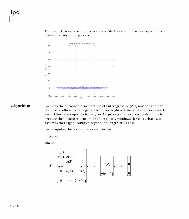
lpc
7-258
The prediction error is approximately white Gaussian noise, as expected for athird-order AR input process.
Algorithm lpc uses the autocorrelation method of autoregressive (AR) modeling to findthe filter coefficients. The generated filter might not model the process exactlyeven if the data sequence is truly an AR process of the correct order. This isbecause the autocorrelation method implicitly windows the data, that is, itassumes that signal samples beyond the length of x are 0.
lpc computes the least squares solution to
where
−5000 −4000 −3000 −2000 −1000 0 1000 2000 3000 4000 5000−0.2
0
0.2
0.4
0.6
0.8
1
1.2Autocorrelation of the Prediction Error
Lags
Nor
mal
ized
Val
ue
Xa b≈
X
x 1( ) 0 0x 2( ) x 1( )
x 2( ) 0x m( ) x 1( )
0 x m( ) x 2( )
0 0 x m( )
= a
1a 2( )
a p 1+( )
= b
10
0
=, ,
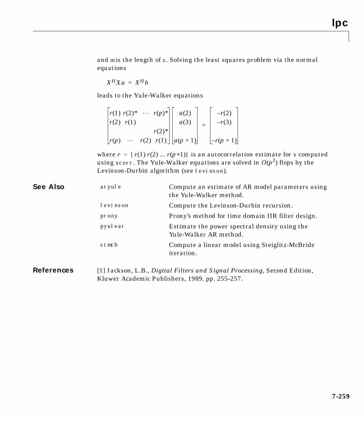
lpc
7-259
and m is the length of x. Solving the least squares problem via the normalequations
leads to the Yule-Walker equations
where r = [r(1) r(2) ... r(p+1)] is an autocorrelation estimate for x computedusing xcorr. The Yule-Walker equations are solved in O(p2) flops by theLevinson-Durbin algorithm (see levinson).
See Also
References [1] Jackson, L.B., Digital Filters and Signal Processing, Second Edition,Kluwer Academic Publishers, 1989. pp. 255-257.
XHXa XHb=
r 1( ) r 2( )* r p( )*r 2( ) r 1( )
r 2( )*r p( ) r 2( ) r 1( )
a 2( )
a 3( )
a p 1+( )
r 2( )–
r 3( )–
r p 1+( )–
=
aryule Compute an estimate of AR model parameters usingthe Yule-Walker method.
levinson Compute the Levinson-Durbin recursion.
prony Prony’s method for time domain IIR filter design.
pyulear Estimate the power spectral density using theYule-Walker AR method.
stmcb Compute a linear model using Steiglitz-McBrideiteration.
lsf2poly
7-260
7lsf2polyPurpose Convert line spectral frequencies to prediction filter coefficients.
Syntax a = lsf2poly(lsf)
Description a = lsf2poly(lsf) returns a vector a containing the prediction filtercoefficients from a vector lsf of line spectral frequencies (also known as linespectrum pairs).
Examples lsf = [0.7842 1.5605 1.8776 1.8984 2.3593];a = lsf2poly(lsf)
a = 1.0000 0.6148 0.9899 0.0001 0.0031 -0.0081
See Also
References [1] Deller, J.R., J.G. Proakis, and J.H.L. Hansen, “Discrete-Time Processing ofSpeech Signals,” Prentice-Hall, 1993.
[2] Rabiner, L.R., and R.W. Schafer, “Digital Processing of Speech Signals,”Prentice-Hall, 1978.
ac2poly Convert autocorrelation parameters to predictionfilter coefficients.
poly2lsf Convert prediction filter coefficients to line spectralfrequencies.
rc2poly Convert reflection coefficients to prediction filtercoefficients.

maxflat
7-261
7maxflatPurpose Generalized digital Butterworth filter design.
Syntax [b,a,] = maxflat(nb,na,Wn)b = maxflat(nb,'sym',Wn)[b,a,b1,b2] = maxflat(nb,na,Wn)[...] = maxflat(nb,na,Wn,'design_flag')
Description [b,a,] = maxflat(nb,na,Wn) is a lowpass Butterworth filter with numeratorand denominator coefficients b and a of orders nb and na respectively. Wn is thenormalized cutoff frequency at which the magnitude response of the filter isequal to (approx. -3 dB). Wnmust be between 0 and 1, where 1 correspondsto the Nyquist frequency.
b = maxflat(nb,'sym',Wn) is a symmetric FIR Butterworth filter. nbmust beeven, and Wn is restricted to a subinterval of [0,1]. The function raises an errorif Wn is specified outside of this subinterval.
[b,a,b1,b2] = maxflat(nb,na,Wn) returns two polynomials b1 and b2whoseproduct is equal to the numerator polynomial b (that is, b = conv(b1,b2)).b1 contains all the zeros at z = -1, and b2 contains all the other zeros.
[...] = maxflat(nb,na,Wn,'design_flag') enables you to monitor the filterdesign, where 'design_flag' is:
• 'trace', for a textual display of the design table used in the design
• 'plots', for plots of the filter’s magnitude, group delay, and zeros and poles
• 'both', for both the textual display and plots
Examples nb = 10; na = 2; Wn = 0.2;[b,a,b1,b2] = maxflat(nb,na,Wn,'plots')
1 2⁄
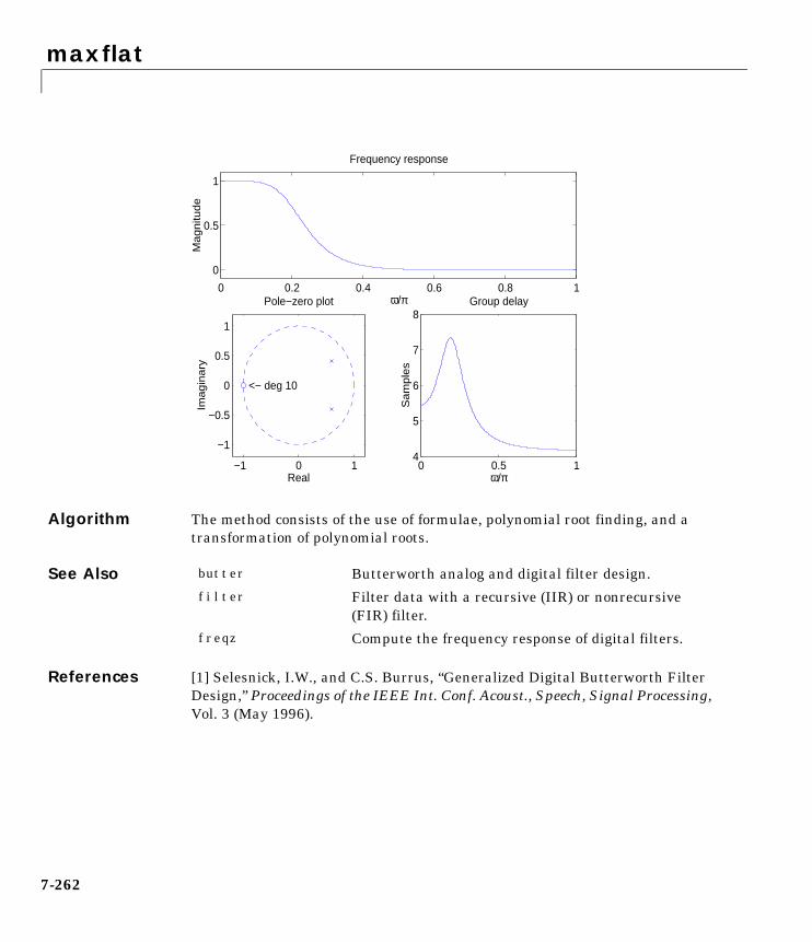
maxflat
7-262
Algorithm The method consists of the use of formulae, polynomial root finding, and atransformation of polynomial roots.
See Also
References [1] Selesnick, I.W., and C.S. Burrus, “Generalized Digital Butterworth FilterDesign,” Proceedings of the IEEE Int. Conf. Acoust., Speech, Signal Processing,Vol. 3 (May 1996).
0 0.2 0.4 0.6 0.8 1
0
0.5
1
ω/π
Ma
gn
itud
e
Frequency response
−1 0 1
−1
−0.5
0
0.5
1
Real
Ima
gin
ary
Pole−zero plot
<− deg 10
0 0.5 14
5
6
7
8
ω/π
Sa
mp
les
Group delay
butter Butterworth analog and digital filter design.
filter Filter data with a recursive (IIR) or nonrecursive(FIR) filter.
freqz Compute the frequency response of digital filters.
medfilt1
7-263
7medfilt1Purpose One-dimensional median filtering.
Syntax y = medfilt1(x,n)y = medfilt1(x,n,blksz)
Description y = medfilt1(x,n) applies an order n one-dimensional median filter tovector x; the function considers the signal to be 0 beyond the end points.Output y has the same length as x.
For n odd, y(k) is the median of x(k-(n-1)/2:k+(n-1)/2).
For n even, y(k) is the median of x(k-n/2), x(k-(n/2)+1), ..., x(k+(n/2)-1).In this case, medfilt1 sorts the numbers, then takes the average of the(n-1)/2 and ((n-1)/2)+1 elements.
The default for n is 3.
y = medfilt1(x,n,blksz) uses a for-loop to compute blksz (block size)output samples at a time. Use blksz << length(x) if you are low on memory,since medfilt1 uses a working matrix of size n-by-blksz. By default,blksz = length(x); this provides the fastest execution if you have sufficientmemory.
If x is a matrix, medfilt1 median filters its columns using
y(:,i) = medfilt1(x(:,i),n,blksz)
in a loop over the columns of x.
See Also
References [1] Pratt, W.K., Digital Image Processing, John Wiley & Sons, 1978,pp. 330-333.
filter Filter data with a recursive (IIR) or nonrecursive(FIR) filter.
medfilt2 Two-dimensional median filtering (see the ImageProcessing Toolbox documentation).
median Median value (see the MATLAB documentation).
modulate
7-264
7modulatePurpose Modulation for communications simulation.
Syntax y = modulate(x,fc,fs,'method')y = modulate(x,fc,fs,'method',opt)[y,t] = modulate(x,fc,fs)
Description y = modulate(x,fc,fs,'method') and
y = modulate(x,fc,fs,'method',opt) modulate the real message signal xwith a carrier frequency fc and sampling frequency fs, using one of the optionslisted below for 'method'. Note that some methods accept an option, opt.
amdsb-scor
am
Amplitude modulation, double sideband, suppressed carrier.Multiplies x by a sinusoid of frequency fc.
y = x.*cos(2*pi*fc*t)
amdsb-tc Amplitude modulation, double sideband, transmitted carrier.Subtracts scalar opt from x and multiplies the result by a sinusoidof frequency fc.
y = (x-opt).*cos(2*pi*fc*t)
If the opt parameter is not present, modulate uses a default ofmin(min(x)) so that the message signal (x-opt) is entirelynonnegative and has a minimum value of 0.
amssb Amplitude modulation, single sideband. Multiplies x by asinusoid of frequency fc and adds the result to the Hilbert transformof x multiplied by a phase shifted sinusoid of frequency fc.
y =x.*cos(2*pi*fc*t)+imag(hilbert(x)).*sin(2*pi*fc*t)
This effectively removes the upper sideband.

modulate
7-265
fm Frequency modulation. Creates a sinusoid with instantaneousfrequency that varies with the message signal x.
y = cos(2*pi*fc*t + opt*cumsum(x))
cumsum is a rectangular approximation to the integral of x.modulate uses opt as the constant of frequency modulation. If optis not present, modulate uses a default of
opt = (fc/fs)*2*pi/(max(max(x)))
so the maximum frequency excursion from fc is fc Hz.
pm Phase modulation. Creates a sinusoid of frequency fc whosephase varies with the message signal x.
y = cos(2*pi*fc*t + opt*x)
modulate uses opt as the constant of phase modulation. If opt isnot present, modulate uses a default of
opt = pi/(max(max(x)))
so the maximum phase excursion is π radians.
pwm Pulse-width modulation. Creates a pulse-width modulatedsignal from the pulse widths in x. The elements of x must bebetween 0 and 1, specifying the width of each pulse in fractions ofa period. The pulses start at the beginning of each period, that is,they are left justified.
modulate(x,fc,fs,'pwm','centered')
yields pulses centered at the beginning of each period. y is length length(x)*fs/fc.
ptm Pulse time modulation. Creates a pulse time modulated signalfrom the pulse times in x. The elements of x must be between 0and 1, specifying the left edge of each pulse in fractions of a period.opt is a scalar between 0 and 1 that specifies the length of eachpulse in fractions of a period. The default for opt is 0.1. y is lengthlength(x)*fs/fc.
qam Quadrature amplitude modulation. Creates a quadratureamplitude modulated signal from signals x and opt.
y = x.*cos(2*pi*fc*t) + opt.*sin(2*pi*fc*t)
opt must be the same size as x.

modulate
7-266
If you do not specify 'method', then modulate assumes am. Except for the pwmand ptm cases, y is the same size as x.
If x is an array, modulate modulates its columns.
[y,t] = modulate(x,fc,fs) returns the internal time vector t that modulateuses in its computations.
See Also demod Demodulation for communications simulation.
vco Voltage controlled oscillator.

pburg
7-267
7pburgPurpose Estimate the power spectral density using the Burg method.
Syntax Pxx = pburg(x,p)[Pxx,w] = pburg(x,p)[Pxx,w] = pburg(x,p,nfft)[Pxx,f] = pburg(x,p,nfft,fs)[Pxx,f] = pburg(x,p,nfft,fs,'range')[Pxx,w] = pburg(x,p,nfft,'range')pburg(...)
Description Pxx = pburg(x,p) implements the Burg algorithm, a parametric spectralestimation method, and returns Pxx, an estimate of the power spectral density(PSD) of the vector x. The entries of x represent samples of a discrete-timesignal, and p is the integer specifying the order of an autoregressive (AR)prediction model for the signal, used in estimating the PSD.
The power spectral density is calculated in units of power per radians persample. Real-valued inputs produce full power one-sided (in frequency) PSDs(by default), while complex-valued inputs produce two-sided PSDs.
In general, the length of the FFT and the values of the input x determine thelength of Pxx and the range of the corresponding normalized frequencies. Forthis syntax, the (default) FFT length is 256. The following table indicates thelength of Pxx and the range of the corresponding normalized frequencies forthis syntax.
[Pxx,w] = pburg(x,p) also returns w, a vector of frequencies at which thePSD is estimated. Pxx and w have the same length. The units for frequency arerad/sample.
Table 7-9: PSD Vector Characteristics for an FFT Length of 256 (Default)
Real/Complex Input Data
Length of Pxx Range of the Corresponding Normalized Frequencies
Real-valued 129 [0, π]
Complex-valued 256 [0, 2π)

pburg
7-268
[Pxx,w] = pburg(x,p,nfft) uses the Burg method to estimate the PSD whilespecifying the length of the FFT with the integer nfft. If you specify nfft asthe empty vector [], it takes the default value of 256.
The length of Pxx and the frequency range for w depend on nfft and the valuesof the input x. The following table indicates the length of Pxx and the frequencyrange for w in this syntax.
[Pxx,f] = pburg(x,p,nfft,fs) uses the sampling frequency fs specified asan integer in hertz (Hz) to compute the PSD vector (Pxx) and the correspondingvector of frequencies (f). In this case, the units for the frequency vector arein Hz. The spectral density produced is calculated in units of power per Hz. Ifyou specify fs as the empty vector [], the sampling frequency defaults to 1 Hz.
The frequency range for f depends on nfft, fs, and the values of the input x.The length of Pxx is the same as in the table above. The following tableindicates the frequency range for f for this syntax.
Table 7-10: PSD and Frequency Vector Characteristics
Real/Complex Input Data
nfft Even/Odd Length of Pxx Range of w
Real-valued Even (nfft/2 + 1) [0, π]
Real-valued Odd (nfft + 1)/2 [0, π)
Complex-valued Even or odd nfft [0, 2π)
Table 7-11: PSD and Frequency Vector Characteristics with fs Specified
Real/Complex Input Data nfft Even/Odd Range of f
Real-valued Even [0,fs/2]
Real-valued Odd [0,fs/2)
Complex-valued Even or odd [0,fs)

pburg
7-269
[Pxx,f] = pburg(x,p,nfft,fs,'range') or
[Pxx,w] = pburg(x,p,nfft,'range') specifies the range of frequency valuesto include in f or w. This syntax is useful when x is real. 'range' can be either:
• 'twosided': Compute the two-sided PSD over the frequency range [0,fs).This is the default for determining the frequency range for complex-valuedx.
- If you specify fs as the empty vector, [], the frequency range is [0,1).
- If you don’t specify fs, the frequency range is [0, 2π).
• 'onesided': Compute the one-sided PSD over the frequency ranges specifiedfor real x. This is the default for determining the frequency range forreal-valued x.
Note You can put the string argument 'range' anywhere in the inputargument list after p.
pburg(...) with no outputs plots the power spectral density in the currentfigure window. The frequency range on the plot is the same as the range ofoutput w (or f) for a given set of parameters.
Examples Because the Burg method estimates the spectral density by fitting an ARprediction model of a given order to the signal, first generate a signal from anAR (all-pole) model of a given order. You can use freqz to check the magnitudeof the frequency response of your AR filter. This will give you an idea of whatto expect when you estimate the PSD using pburg.
a = [1 -2.2137 2.9403 -2.1697 0.9606]; % AR filter coefficientsfreqz(1,a) % AR filter frequency responsetitle('AR System Frequency Response')
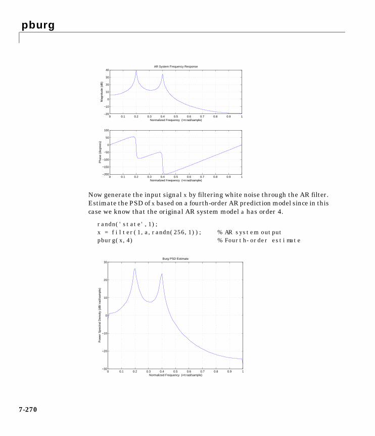
pburg
7-270
Now generate the input signal x by filtering white noise through the AR filter.Estimate the PSD of x based on a fourth-order AR prediction model since in thiscase we know that the original AR system model a has order 4.
randn('state',1);x = filter(1,a,randn(256,1)); % AR system outputpburg(x,4) % Fourth-order estimate
0 0.1 0.2 0.3 0.4 0.5 0.6 0.7 0.8 0.9 1−200
−150
−100
−50
0
50
100
Normalized Frequency (×π rad/sample)
Pha
se (
degr
ees)
0 0.1 0.2 0.3 0.4 0.5 0.6 0.7 0.8 0.9 1−20
−10
0
10
20
30
40
Normalized Frequency (×π rad/sample)
Mag
nitu
de (
dB)
AR System Frequency Response
0 0.1 0.2 0.3 0.4 0.5 0.6 0.7 0.8 0.9 1−30
−20
−10
0
10
20
30
Normalized Frequency (×π rad/sample)
Pow
er S
pect
ral D
ensi
ty (
dB/ r
ad/s
ampl
e)
Burg PSD Estimate
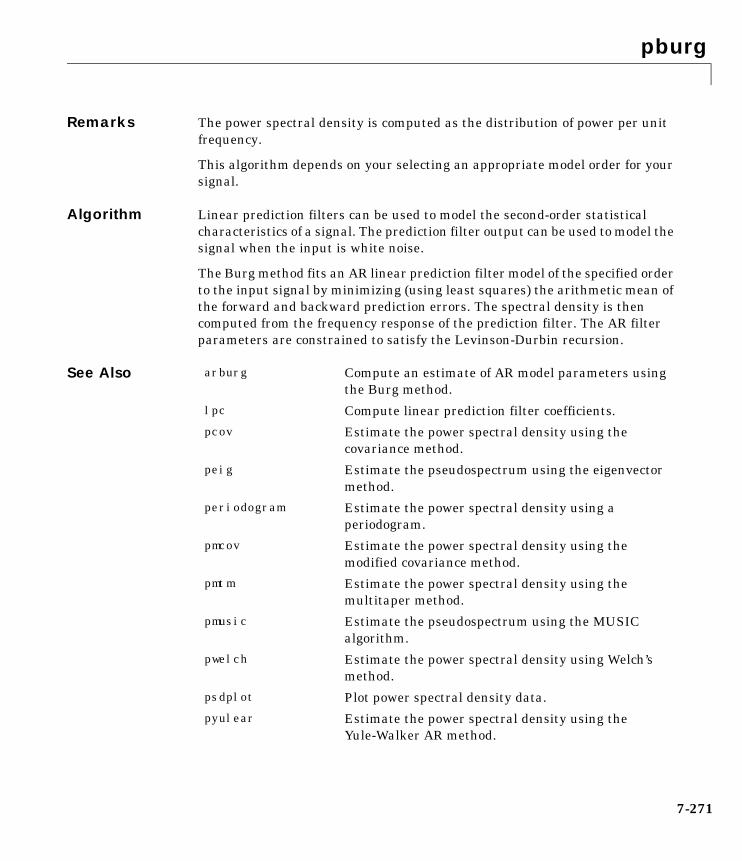
pburg
7-271
Remarks The power spectral density is computed as the distribution of power per unitfrequency.
This algorithm depends on your selecting an appropriate model order for yoursignal.
Algorithm Linear prediction filters can be used to model the second-order statisticalcharacteristics of a signal. The prediction filter output can be used to model thesignal when the input is white noise.
The Burg method fits an AR linear prediction filter model of the specified orderto the input signal by minimizing (using least squares) the arithmetic mean ofthe forward and backward prediction errors. The spectral density is thencomputed from the frequency response of the prediction filter. The AR filterparameters are constrained to satisfy the Levinson-Durbin recursion.
See Also arburg Compute an estimate of AR model parameters usingthe Burg method.
lpc Compute linear prediction filter coefficients.
pcov Estimate the power spectral density using thecovariance method.
peig Estimate the pseudospectrum using the eigenvectormethod.
periodogram Estimate the power spectral density using aperiodogram.
pmcov Estimate the power spectral density using themodified covariance method.
pmtm Estimate the power spectral density using themultitaper method.
pmusic Estimate the pseudospectrum using the MUSICalgorithm.
pwelch Estimate the power spectral density using Welch’smethod.
psdplot Plot power spectral density data.
pyulear Estimate the power spectral density using theYule-Walker AR method.

pburg
7-272
References [1] Marple, S.L. Digital Spectral Analysis, Englewood Cliffs, NJ, Prentice-Hall,1987, Chapter 7.
[2] Stoica, P., and R.L. Moses, Introduction to Spectral Analysis, Prentice-Hall,1997.
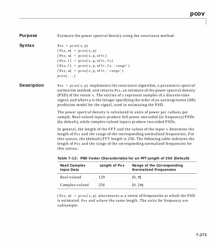
pcov
7-273
7pcovPurpose Estimate the power spectral density using the covariance method.
Syntax Pxx = pcov(x,p)[Pxx,w] = pcov(x,p)[Pxx,w] = pcov(x,p,nfft)[Pxx,f] = pcov(x,p,nfft,fs)[Pxx,f] = pcov(x,p,nfft,fs,'range')[Pxx,w] = pcov(x,p,nfft,'range')pcov(...)
Description Pxx = pcov(x,p) implements the covariance algorithm, a parametric spectralestimation method, and returns Pxx, an estimate of the power spectral density(PSD) of the vector x. The entries of x represent samples of a discrete-timesignal, and where p is the integer specifying the order of an autoregressive (AR)prediction model for the signal, used in estimating the PSD.
The power spectral density is calculated in units of power per radians persample. Real-valued inputs produce full power one-sided (in frequency) PSDs(by default), while complex-valued inputs produce two-sided PSDs.
In general, the length of the FFT and the values of the input x determine thelength of Pxx and the range of the corresponding normalized frequencies. Forthis syntax, the (default) FFT length is 256. The following table indicates thelength of Pxx and the range of the corresponding normalized frequencies forthis syntax.
[Pxx,w] = pcov(x,p) also returns w, a vector of frequencies at which the PSDis estimated. Pxx and w have the same length. The units for frequency arerad/sample.
Table 7-12: PSD Vector Characteristics for an FFT Length of 256 (Default)
Real/Complex Input Data
Length of Pxx Range of the Corresponding Normalized Frequencies
Real-valued 129 [0, π]
Complex-valued 256 [0, 2π)
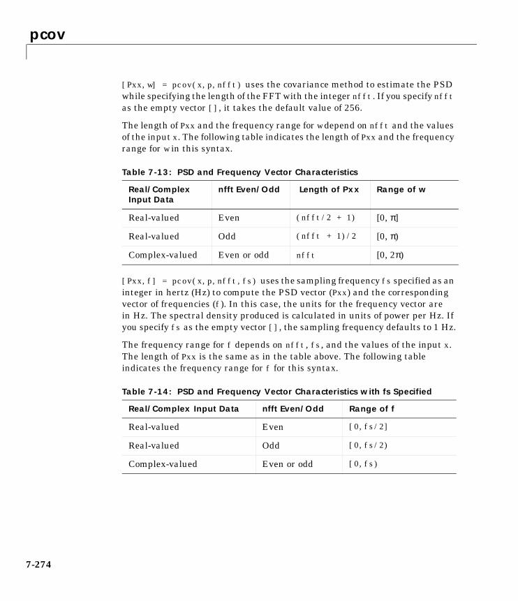
pcov
7-274
[Pxx,w] = pcov(x,p,nfft) uses the covariance method to estimate the PSDwhile specifying the length of the FFT with the integer nfft. If you specify nfftas the empty vector [], it takes the default value of 256.
The length of Pxx and the frequency range for w depend on nfft and the valuesof the input x. The following table indicates the length of Pxx and the frequencyrange for w in this syntax.
[Pxx,f] = pcov(x,p,nfft,fs) uses the sampling frequency fs specified as aninteger in hertz (Hz) to compute the PSD vector (Pxx) and the correspondingvector of frequencies (f). In this case, the units for the frequency vector arein Hz. The spectral density produced is calculated in units of power per Hz. Ifyou specify fs as the empty vector [], the sampling frequency defaults to 1 Hz.
The frequency range for f depends on nfft, fs, and the values of the input x.The length of Pxx is the same as in the table above. The following tableindicates the frequency range for f for this syntax.
Table 7-13: PSD and Frequency Vector Characteristics
Real/Complex Input Data
nfft Even/Odd Length of Pxx Range of w
Real-valued Even (nfft/2 + 1) [0, π]
Real-valued Odd (nfft + 1)/2 [0, π)
Complex-valued Even or odd nfft [0, 2π)
Table 7-14: PSD and Frequency Vector Characteristics with fs Specified
Real/Complex Input Data nfft Even/Odd Range of f
Real-valued Even [0,fs/2]
Real-valued Odd [0,fs/2)
Complex-valued Even or odd [0,fs)
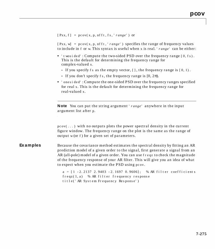
pcov
7-275
[Pxx,f] = pcov(x,p,nfft,fs,'range') or
[Pxx,w] = pcov(x,p,nfft,'range') specifies the range of frequency valuesto include in f or w. This syntax is useful when x is real. 'range' can be either:
• 'twosided': Compute the two-sided PSD over the frequency range [0,fs).This is the default for determining the frequency range forcomplex-valued x.
- If you specify fs as the empty vector, [], the frequency range is [0,1).
- If you don’t specify fs, the frequency range is [0, 2π).
• 'onesided': Compute the one-sided PSD over the frequency ranges specifiedfor real x. This is the default for determining the frequency range forreal-valued x.
Note You can put the string argument 'range' anywhere in the inputargument list after p.
pcov(...) with no outputs plots the power spectral density in the currentfigure window. The frequency range on the plot is the same as the range ofoutput w (or f) for a given set of parameters.
Examples Because the covariance method estimates the spectral density by fitting an ARprediction model of a given order to the signal, first generate a signal from anAR (all-pole) model of a given order. You can use freqz to check the magnitudeof the frequency response of your AR filter. This will give you an idea of whatto expect when you estimate the PSD using pcov.
a = [1 -2.2137 2.9403 -2.1697 0.9606]; % AR filter coefficientsfreqz(1,a) % AR filter frequency responsetitle('AR System Frequency Response')
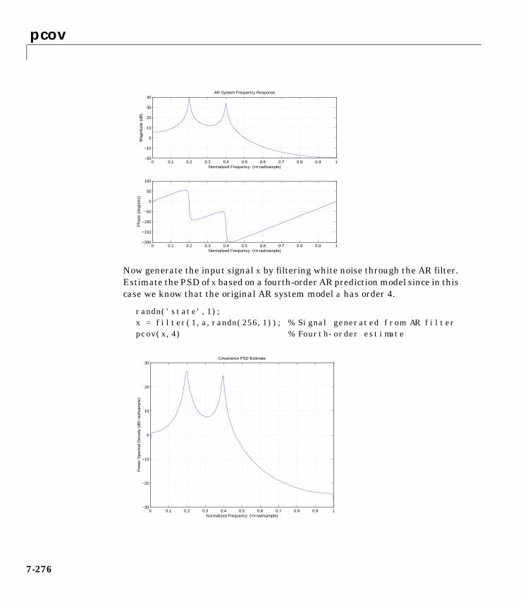
pcov
7-276
Now generate the input signal x by filtering white noise through the AR filter.Estimate the PSD of x based on a fourth-order AR prediction model since in thiscase we know that the original AR system model a has order 4.
randn('state',1);x = filter(1,a,randn(256,1)); % Signal generated from AR filter pcov(x,4) % Fourth-order estimate
0 0.1 0.2 0.3 0.4 0.5 0.6 0.7 0.8 0.9 1−200
−150
−100
−50
0
50
100
Normalized Frequency (×π rad/sample)
Pha
se (
degr
ees)
0 0.1 0.2 0.3 0.4 0.5 0.6 0.7 0.8 0.9 1−20
−10
0
10
20
30
40
Normalized Frequency (×π rad/sample)
Mag
nitu
de (
dB)
AR System Frequency Response
0 0.1 0.2 0.3 0.4 0.5 0.6 0.7 0.8 0.9 1−30
−20
−10
0
10
20
30
Normalized Frequency (×π rad/sample)
Pow
er S
pect
ral D
ensi
ty (
dB/ r
ad/s
ampl
e)
Covariance PSD Estimate

pcov
7-277
Remarks The power spectral density is computed as the distribution of power per unitfrequency.
This algorithm depends on your selecting an appropriate model order for yoursignal.
Algorithm Linear prediction filters can be used to model the second-order statisticalcharacteristics of a signal. The prediction filter output can be used to model thesignal when the input is white noise.
The covariance method estimates the PSD of a signal using the covariancemethod. The covariance (or nonwindowed) method fits an AR linear predictionfilter model to the signal by minimizing the forward prediction error (based oncausal observations of your input signal) in the least squares sense. Thespectral estimate returned by pcov is the squared magnitude of the frequencyresponse of this AR model.
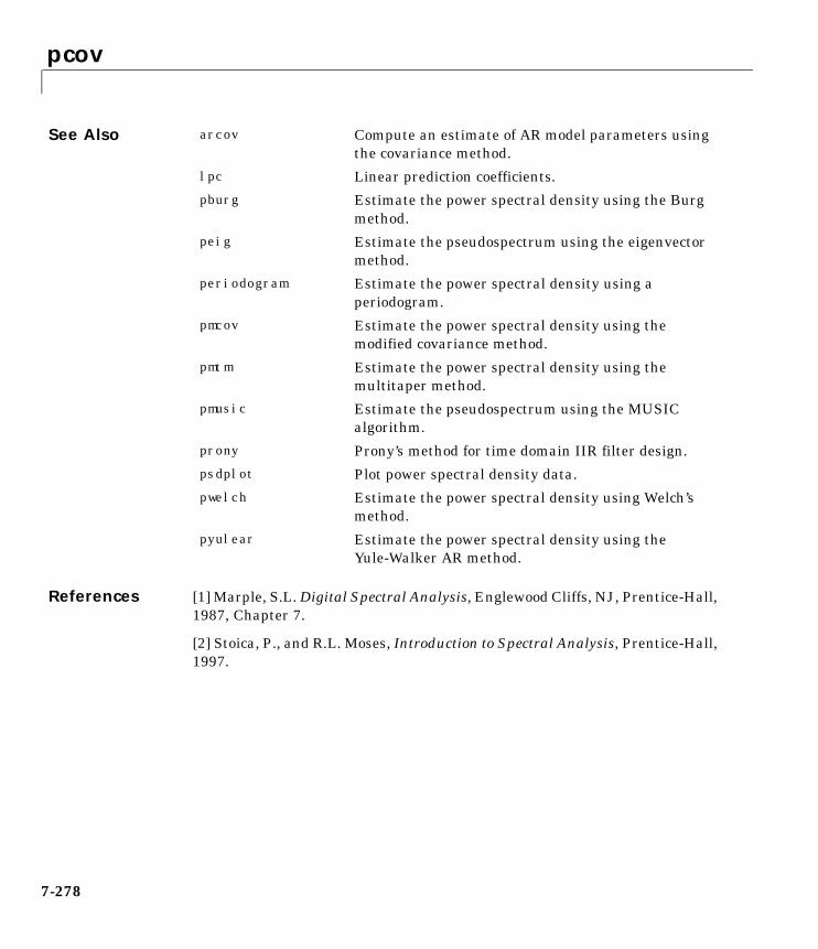
pcov
7-278
See Also
References [1] Marple, S.L. Digital Spectral Analysis, Englewood Cliffs, NJ, Prentice-Hall,1987, Chapter 7.
[2] Stoica, P., and R.L. Moses, Introduction to Spectral Analysis, Prentice-Hall,1997.
arcov Compute an estimate of AR model parameters usingthe covariance method.
lpc Linear prediction coefficients.
pburg Estimate the power spectral density using the Burgmethod.
peig Estimate the pseudospectrum using the eigenvectormethod.
periodogram Estimate the power spectral density using aperiodogram.
pmcov Estimate the power spectral density using themodified covariance method.
pmtm Estimate the power spectral density using themultitaper method.
pmusic Estimate the pseudospectrum using the MUSICalgorithm.
prony Prony’s method for time domain IIR filter design.
psdplot Plot power spectral density data.
pwelch Estimate the power spectral density using Welch’smethod.
pyulear Estimate the power spectral density using theYule-Walker AR method.
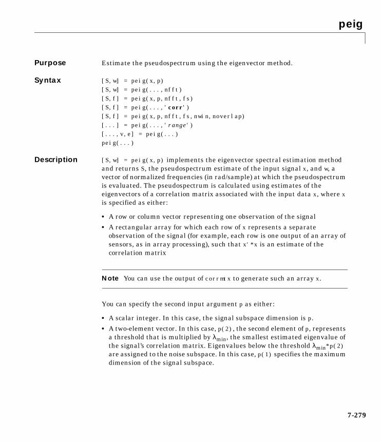
peig
7-279
7peigPurpose Estimate the pseudospectrum using the eigenvector method.
Syntax [S,w] = peig(x,p)[S,w] = peig(...,nfft)[S,f] = peig(x,p,nfft,fs)[S,f] = peig(...,'corr')[S,f] = peig(x,p,nfft,fs,nwin,noverlap)[...] = peig(...,'range')[...,v,e] = peig(...)peig(...)
Description [S,w] = peig(x,p) implements the eigenvector spectral estimation methodand returns S, the pseudospectrum estimate of the input signal x, and w, avector of normalized frequencies (in rad/sample) at which the pseudospectrumis evaluated. The pseudospectrum is calculated using estimates of theeigenvectors of a correlation matrix associated with the input data x, where xis specified as either:
• A row or column vector representing one observation of the signal
• A rectangular array for which each row of x represents a separateobservation of the signal (for example, each row is one output of an array ofsensors, as in array processing), such that x'*x is an estimate of thecorrelation matrix
Note You can use the output of corrmtx to generate such an array x.
You can specify the second input argument p as either:
• A scalar integer. In this case, the signal subspace dimension is p.
• A two-element vector. In this case, p(2), the second element of p, representsa threshold that is multiplied by λmin, the smallest estimated eigenvalue ofthe signal’s correlation matrix. Eigenvalues below the threshold λmin*p(2)are assigned to the noise subspace. In this case, p(1) specifies the maximumdimension of the signal subspace.
peig
7-280
The extra threshold parameter in the second entry in p provides you moreflexibility and control in assigning the noise and signal subspaces.
S and w have the same length. In general, the length of the FFT and the valuesof the input x determine the length of the computed S and the range of thecorresponding normalized frequencies. The following table indicates the lengthof S (and w) and the range of the corresponding normalized frequencies for thissyntax.
[S,w] = peig(...,nfft) specifies the length of the FFT used to estimate thepseudospectrum with the integer nfft. The default value for nfft (entered asan empty vector []) is 256.
The following table indicates the length of S and w, and the frequency rangefor w for this syntax.
[S,f] = peig(x,p,nfft,fs)) returns the pseudospectrum in the vector Sevaluated at the corresponding vector of frequencies f (in Hz). You supply thesampling frequency fs in Hz. If you specify fs with the empty vector [], thesampling frequency defaults to 1 Hz.
Table 7-15: S Characteristics for an FFT Length of 256 (Default)
Real/Complex Input Data
Length of S and w Range of the Corresponding Normalized Frequencies
Real-valued 129 [0, π]
Complex-valued 256 [0, 2π)
Table 7-16: S and Frequency Vector Characteristics
Real/Complex Input Data
nfft Even/Odd Length of S and w
Range of w
Real-valued Even (nfft/2 + 1) [0, π]
Real-valued Odd (nfft + 1)/2 [0, π)
Complex-valued Even or odd nfft [0, 2π)
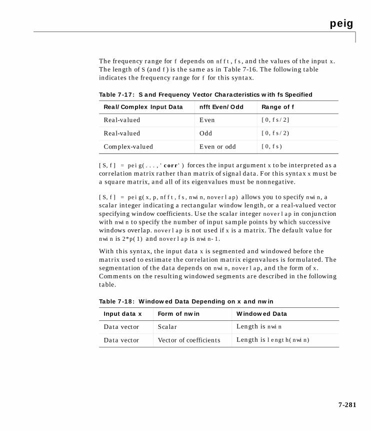
peig
7-281
The frequency range for f depends on nfft, fs, and the values of the input x.The length of S (and f) is the same as in Table 7-16. The following tableindicates the frequency range for f for this syntax.
[S,f] = peig(...,'corr') forces the input argument x to be interpreted as acorrelation matrix rather than matrix of signal data. For this syntax x must bea square matrix, and all of its eigenvalues must be nonnegative.
[S,f] = peig(x,p,nfft,fs,nwin,noverlap) allows you to specify nwin, ascalar integer indicating a rectangular window length, or a real-valued vectorspecifying window coefficients. Use the scalar integer noverlap in conjunctionwith nwin to specify the number of input sample points by which successivewindows overlap. noverlap is not used if x is a matrix. The default value fornwin is 2*p(1) and noverlap is nwin-1.
With this syntax, the input data x is segmented and windowed before thematrix used to estimate the correlation matrix eigenvalues is formulated. Thesegmentation of the data depends on nwin, noverlap, and the form of x.Comments on the resulting windowed segments are described in the followingtable.
Table 7-17: S and Frequency Vector Characteristics with fs Specified
Real/Complex Input Data nfft Even/Odd Range of f
Real-valued Even [0,fs/2]
Real-valued Odd [0,fs/2)
Complex-valued Even or odd [0,fs)
Table 7-18: Windowed Data Depending on x and nwin
Input data x Form of nwin Windowed Data
Data vector Scalar Length is nwin
Data vector Vector of coefficients Length is length(nwin)
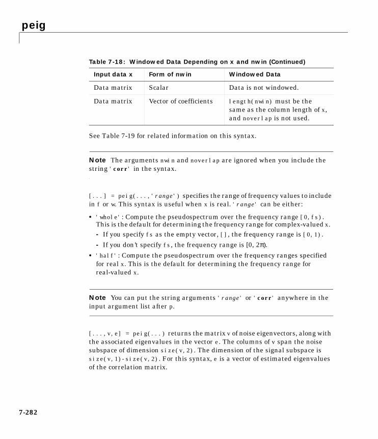
peig
7-282
See Table 7-19 for related information on this syntax.
Note The arguments nwin and noverlap are ignored when you include thestring 'corr' in the syntax.
[...] = peig(...,'range') specifies the range of frequency values to includein f or w. This syntax is useful when x is real. 'range' can be either:
• 'whole': Compute the pseudospectrum over the frequency range [0,fs).This is the default for determining the frequency range for complex-valued x. - If you specify fs as the empty vector, [], the frequency range is [0,1).
- If you don’t specify fs, the frequency range is [0, 2π).
• 'half': Compute the pseudospectrum over the frequency ranges specifiedfor real x. This is the default for determining the frequency range forreal-valued x.
Note You can put the string arguments 'range' or 'corr' anywhere in theinput argument list after p.
[...,v,e] = peig(...) returns the matrix v of noise eigenvectors, along withthe associated eigenvalues in the vector e. The columns of v span the noisesubspace of dimension size(v,2). The dimension of the signal subspace issize(v,1)-size(v,2). For this syntax, e is a vector of estimated eigenvaluesof the correlation matrix.
Data matrix Scalar Data is not windowed.
Data matrix Vector of coefficients length(nwin) must be thesame as the column length of x,and noverlap is not used.
Table 7-18: Windowed Data Depending on x and nwin (Continued)
Input data x Form of nwin Windowed Data

peig
7-283
peig(...) with no output arguments plots the pseudospectrum in the currentfigure window.
Remarks In the process of estimating the pseudospectrum, peig computes the noise andsignal subspaces from the estimated eigenvectors vj and eigenvalues λj of thesignal’s correlation matrix. The smallest of these eigenvalues is used inconjunction with the threshold parameter p(2) to affect the dimension of thenoise subspace in some cases.
The length n of the eigenvectors computed by peig is the sum of the dimensionsof the signal and noise subspaces. This eigenvector length depends on yourinput (signal data or correlation matrix) and the syntax you use.
The following table summarizes the dependency of the eigenvector length onthe input argument.
You should specify nwin > p(1) or length(nwin) > p(1) if you want p(2) > 1 tohave any effect.
Table 7-19: Eigenvector Length Depending on Input Data and Syntax
Form of Input Data x Comments on the Syntax Length n of Eigenvectors
Row or column vector nwin is specified as a scalarinteger.
nwin
Row or column vector nwin is specified as a vector. length(nwin)
Row or column vector nwin is not specified. 2*p(1)
l-by-m matrix If nwin is specified as ascalar, it is not used. If nwinis specified as a vector,length(nwin) must equalm.
m
m-by-m nonnegativedefinite matrix
The string 'corr' isspecified and nwin is notused.
m

peig
7-284
Examples Implement the eigenvector method to find the pseudospectrum of the sum ofthree sinusoids in noise, using the default FFT length of 256. Use the modifiedcovariance method for the correlation matrix estimate.
randn('state',1); n=0:99; s=exp(i*pi/2*n)+2*exp(i*pi/4*n)+exp(i*pi/3*n)+randn(1,100); X=corrmtx(s,12,'mod'); peig(X,3,'whole') % Uses the default NFFT of 256.
Algorithm The eigenvector method estimates the pseudospectrum from a signal or acorrelation matrix using a weighted version of the MUSIC algorithm derivedfrom Schmidt’s eigenspace analysis method [1][2]. The algorithm performseigenspace analysis of the signal’s correlation matrix in order to estimate thesignal’s frequency content. The eigenvalues and eigenvectors of the signal’scorrelation matrix are estimated using svd if you don’t supply the correlationmatrix. This algorithm is particularly suitable for signals that are the sum ofsinusoids with additive white Gaussian noise.
0 0.2 0.4 0.6 0.8 1 1.2 1.4 1.6 1.8−15
−10
−5
0
5
10
15
20
25
30
Normalized Frequency (×π rad/sample)
dB
Eigenvector Method Pseudospectrum
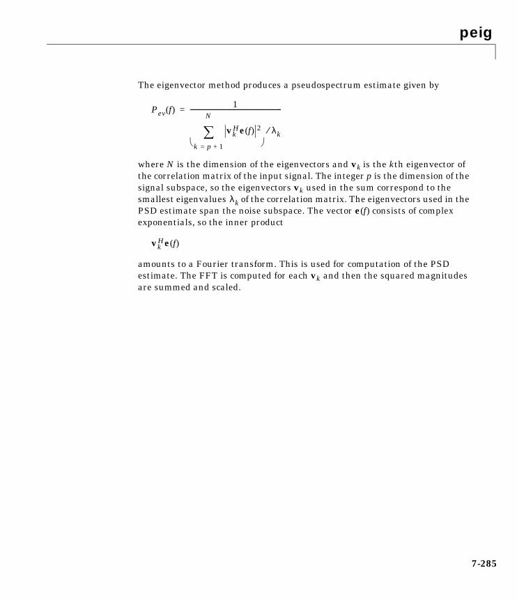
peig
7-285
The eigenvector method produces a pseudospectrum estimate given by
where N is the dimension of the eigenvectors and vk is the kth eigenvector ofthe correlation matrix of the input signal. The integer p is the dimension of thesignal subspace, so the eigenvectors vk used in the sum correspond to thesmallest eigenvalues of the correlation matrix. The eigenvectors used in thePSD estimate span the noise subspace. The vector e(f) consists of complexexponentials, so the inner product
amounts to a Fourier transform. This is used for computation of the PSDestimate. The FFT is computed for each vk and then the squared magnitudesare summed and scaled.
Pev f( )1
vkHe f( ) 2
k p 1+=
N
λk⁄
-----------------------------------------------------------=
λk
vkHe f( )
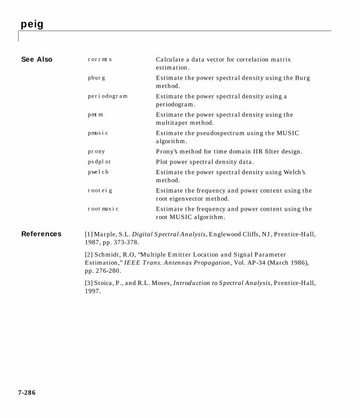
peig
7-286
See Also
References [1] Marple, S.L. Digital Spectral Analysis, Englewood Cliffs, NJ, Prentice-Hall,1987, pp. 373-378.
[2] Schmidt, R.O, “Multiple Emitter Location and Signal ParameterEstimation,” IEEE Trans. Antennas Propagation, Vol. AP-34 (March 1986),pp. 276-280.
[3] Stoica, P., and R.L. Moses, Introduction to Spectral Analysis, Prentice-Hall,1997.
corrmtx Calculate a data vector for correlation matrixestimation.
pburg Estimate the power spectral density using the Burgmethod.
periodogram Estimate the power spectral density using aperiodogram.
pmtm Estimate the power spectral density using themultitaper method.
pmusic Estimate the pseudospectrum using the MUSICalgorithm.
prony Prony’s method for time domain IIR filter design.
psdplot Plot power spectral density data.
pwelch Estimate the power spectral density using Welch’smethod.
rooteig Estimate the frequency and power content using theroot eigenvector method.
rootmusic Estimate the frequency and power content using theroot MUSIC algorithm.
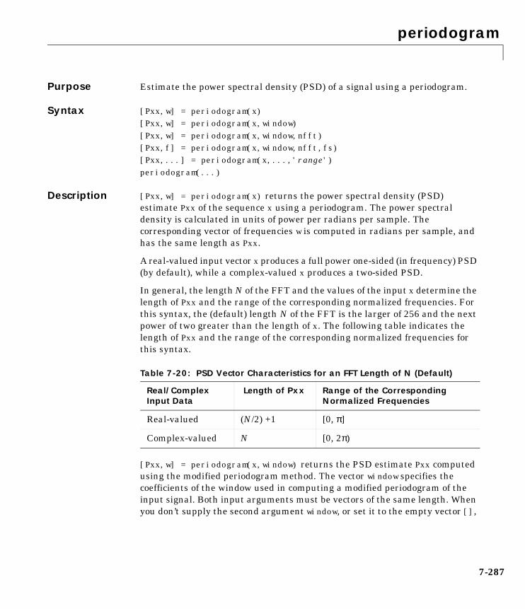
periodogram
7-287
7periodogramPurpose Estimate the power spectral density (PSD) of a signal using a periodogram.
Syntax [Pxx,w] = periodogram(x)[Pxx,w] = periodogram(x,window)[Pxx,w] = periodogram(x,window,nfft)[Pxx,f] = periodogram(x,window,nfft,fs)[Pxx,...] = periodogram(x,...,'range')periodogram(...)
Description [Pxx,w] = periodogram(x) returns the power spectral density (PSD)estimate Pxx of the sequence x using a periodogram. The power spectraldensity is calculated in units of power per radians per sample. Thecorresponding vector of frequencies w is computed in radians per sample, andhas the same length as Pxx.
A real-valued input vector x produces a full power one-sided (in frequency) PSD(by default), while a complex-valued x produces a two-sided PSD.
In general, the length N of the FFT and the values of the input x determine thelength of Pxx and the range of the corresponding normalized frequencies. Forthis syntax, the (default) length N of the FFT is the larger of 256 and the nextpower of two greater than the length of x. The following table indicates thelength of Pxx and the range of the corresponding normalized frequencies forthis syntax.
[Pxx,w] = periodogram(x,window) returns the PSD estimate Pxx computedusing the modified periodogram method. The vector window specifies thecoefficients of the window used in computing a modified periodogram of theinput signal. Both input arguments must be vectors of the same length. Whenyou don’t supply the second argument window, or set it to the empty vector [],
Table 7-20: PSD Vector Characteristics for an FFT Length of N (Default)
Real/Complex Input Data
Length of Pxx Range of the Corresponding Normalized Frequencies
Real-valued (N/2) +1 [0, π]
Complex-valued N [0, 2π)
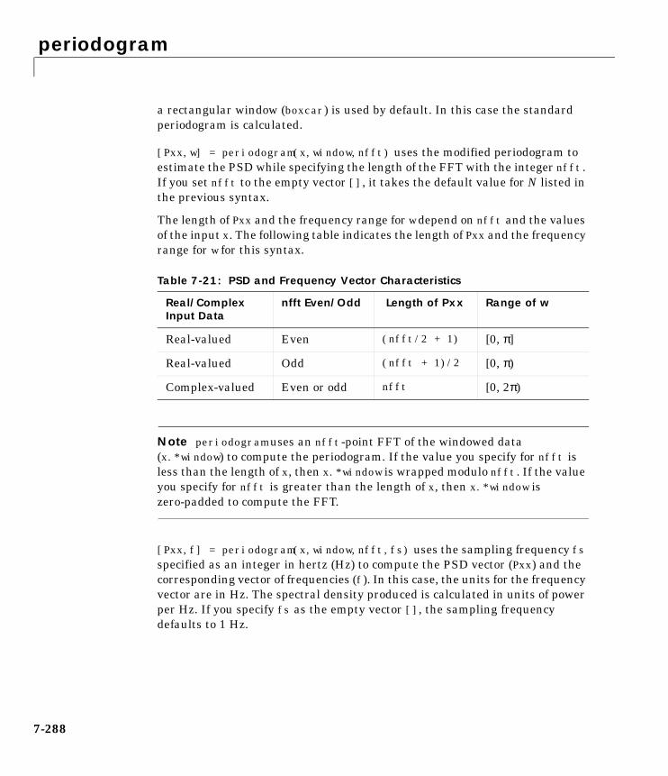
periodogram
7-288
a rectangular window (boxcar) is used by default. In this case the standardperiodogram is calculated.
[Pxx,w] = periodogram(x,window,nfft) uses the modified periodogram toestimate the PSD while specifying the length of the FFT with the integer nfft.If you set nfft to the empty vector [], it takes the default value for N listed inthe previous syntax.
The length of Pxx and the frequency range for w depend on nfft and the valuesof the input x. The following table indicates the length of Pxx and the frequencyrange for w for this syntax.
Note periodogram uses an nfft-point FFT of the windowed data(x.*window) to compute the periodogram. If the value you specify for nfft isless than the length of x, then x.*window is wrapped modulo nfft. If the valueyou specify for nfft is greater than the length of x, then x.*window iszero-padded to compute the FFT.
[Pxx,f] = periodogram(x,window,nfft,fs) uses the sampling frequency fsspecified as an integer in hertz (Hz) to compute the PSD vector (Pxx) and thecorresponding vector of frequencies (f). In this case, the units for the frequencyvector are in Hz. The spectral density produced is calculated in units of powerper Hz. If you specify fs as the empty vector [], the sampling frequencydefaults to 1 Hz.
Table 7-21: PSD and Frequency Vector Characteristics
Real/Complex Input Data
nfft Even/Odd Length of Pxx Range of w
Real-valued Even (nfft/2 + 1) [0, π]
Real-valued Odd (nfft + 1)/2 [0, π)
Complex-valued Even or odd nfft [0, 2π)
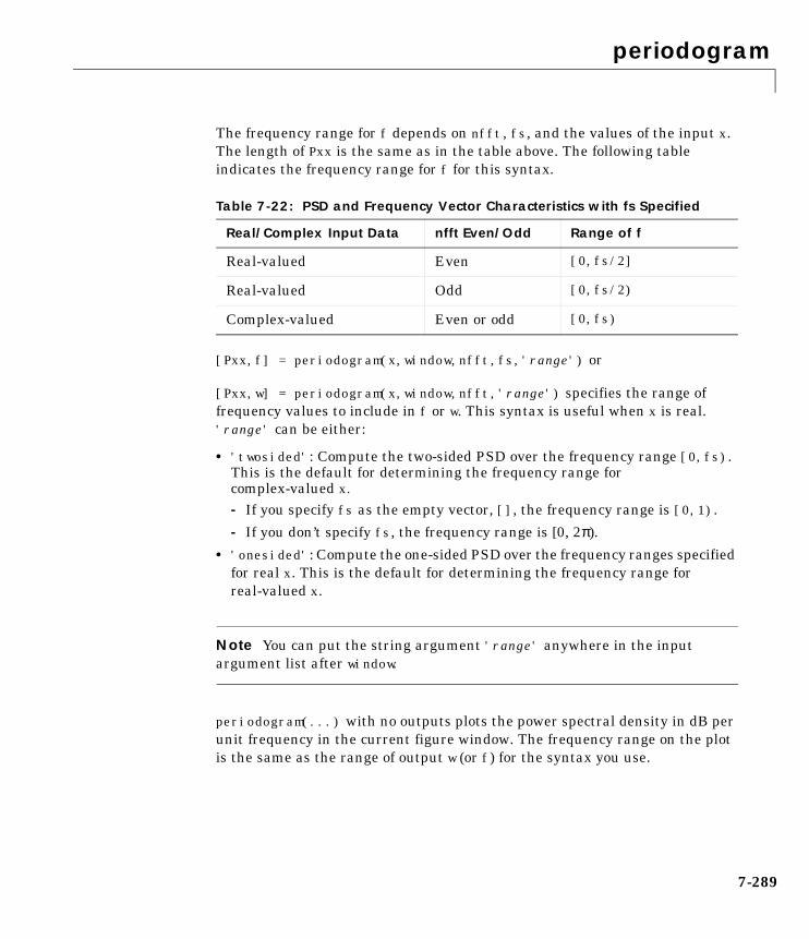
periodogram
7-289
The frequency range for f depends on nfft, fs, and the values of the input x.The length of Pxx is the same as in the table above. The following tableindicates the frequency range for f for this syntax.
[Pxx,f] = periodogram(x,window,nfft,fs,'range') or
[Pxx,w] = periodogram(x,window,nfft,'range') specifies the range offrequency values to include in f or w. This syntax is useful when x is real.'range' can be either:
• 'twosided': Compute the two-sided PSD over the frequency range [0,fs).This is the default for determining the frequency range forcomplex-valued x.
- If you specify fs as the empty vector, [], the frequency range is [0,1).
- If you don’t specify fs, the frequency range is [0, 2π).
• 'onesided': Compute the one-sided PSD over the frequency ranges specifiedfor real x. This is the default for determining the frequency range forreal-valued x.
Note You can put the string argument 'range' anywhere in the inputargument list after window.
periodogram(...) with no outputs plots the power spectral density in dB perunit frequency in the current figure window. The frequency range on the plotis the same as the range of output w (or f) for the syntax you use.
Table 7-22: PSD and Frequency Vector Characteristics with fs Specified
Real/Complex Input Data nfft Even/Odd Range of f
Real-valued Even [0,fs/2]
Real-valued Odd [0,fs/2)
Complex-valued Even or odd [0,fs)
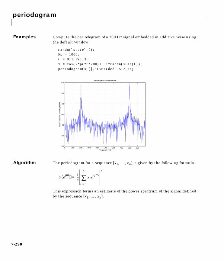
periodogram
7-290
Examples Compute the periodogram of a 200 Hz signal embedded in additive noise usingthe default window.
randn('state',0);Fs = 1000; t = 0:1/Fs:.3;x = cos(2*pi*t*200)+0.1*randn(size(t)); periodogram(x,[],'twosided',512,Fs)
Algorithm The periodogram for a sequence [x1, ... , xn] is given by the following formula.
This expression forms an estimate of the power spectrum of the signal definedby the sequence [x1, ... , xn].
0 100 200 300 400 500 600 700 800 900−70
−60
−50
−40
−30
−20
−10
Frequency (Hz)
Pow
er S
pect
ral D
ensi
ty (
dB/H
z)
Periodogram PSD Estimate
S ejω( ) 1n--- xle
jωl–
l 1=
n
2
=
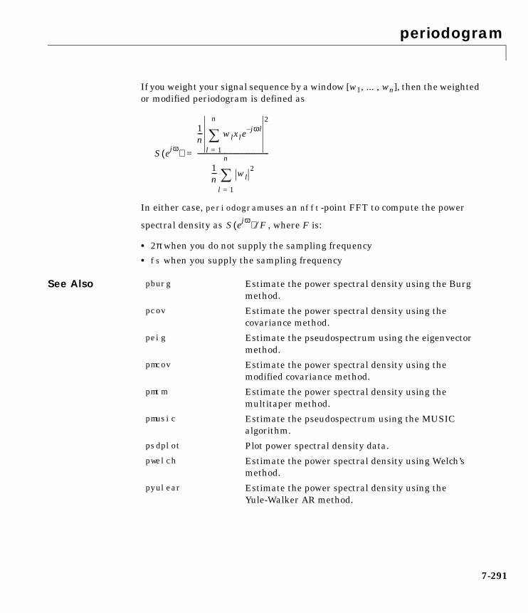
periodogram
7-291
If you weight your signal sequence by a window [w1, ... , wn], then the weightedor modified periodogram is defined as
In either case, periodogram uses an nfft-point FFT to compute the power
spectral density as , where F is:
• 2π when you do not supply the sampling frequency
• fs when you supply the sampling frequency
See Also
S ejω( )
1n--- wlxle
jωl–
l 1=
n
2
1n--- wl
2
l 1=
n
---------------------------------------------=
S ejω( ) F⁄
pburg Estimate the power spectral density using the Burgmethod.
pcov Estimate the power spectral density using thecovariance method.
peig Estimate the pseudospectrum using the eigenvectormethod.
pmcov Estimate the power spectral density using themodified covariance method.
pmtm Estimate the power spectral density using themultitaper method.
pmusic Estimate the pseudospectrum using the MUSICalgorithm.
psdplot Plot power spectral density data.
pwelch Estimate the power spectral density using Welch’smethod.
pyulear Estimate the power spectral density using theYule-Walker AR method.
periodogram
7-292
References [1] Stoica, P., and R.L. Moses, Introduction to Spectral Analysis, Prentice-Hall,1997, pp. 24-26.
[2] Welch, P.D, “The Use of Fast Fourier Transform for the Estimation of PowerSpectra: A Method Based on Time Averaging Over Short, ModifiedPeriodograms,” IEEE Trans. Audio Electroacoustics, Vol. AU-15 (June 1967),pp. 70-73.
[3] Oppenheim, A.V., and R.W. Schafer, Discrete-Time Signal Processing,Prentice-Hall, 1989, pp. 730-742.
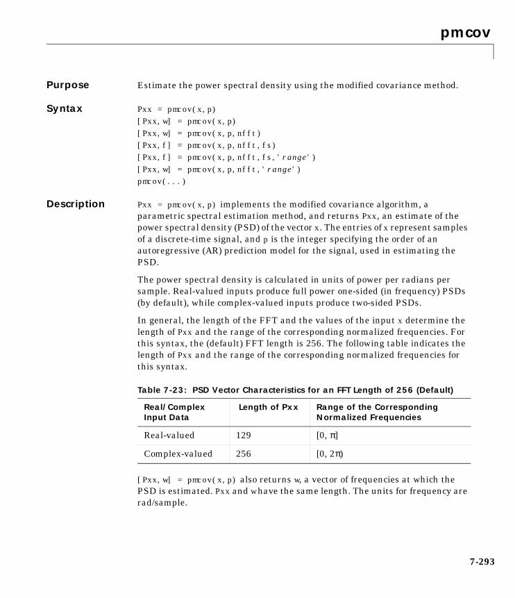
pmcov
7-293
7pmcovPurpose Estimate the power spectral density using the modified covariance method.
Syntax Pxx = pmcov(x,p)[Pxx,w] = pmcov(x,p)[Pxx,w] = pmcov(x,p,nfft)[Pxx,f] = pmcov(x,p,nfft,fs)[Pxx,f] = pmcov(x,p,nfft,fs,'range')[Pxx,w] = pmcov(x,p,nfft,'range')pmcov(...)
Description Pxx = pmcov(x,p) implements the modified covariance algorithm, aparametric spectral estimation method, and returns Pxx, an estimate of thepower spectral density (PSD) of the vector x. The entries of x represent samplesof a discrete-time signal, and p is the integer specifying the order of anautoregressive (AR) prediction model for the signal, used in estimating thePSD.
The power spectral density is calculated in units of power per radians persample. Real-valued inputs produce full power one-sided (in frequency) PSDs(by default), while complex-valued inputs produce two-sided PSDs.
In general, the length of the FFT and the values of the input x determine thelength of Pxx and the range of the corresponding normalized frequencies. Forthis syntax, the (default) FFT length is 256. The following table indicates thelength of Pxx and the range of the corresponding normalized frequencies forthis syntax.
[Pxx,w] = pmcov(x,p) also returns w, a vector of frequencies at which thePSD is estimated. Pxx and w have the same length. The units for frequency arerad/sample.
Table 7-23: PSD Vector Characteristics for an FFT Length of 256 (Default)
Real/Complex Input Data
Length of Pxx Range of the Corresponding Normalized Frequencies
Real-valued 129 [0, π]
Complex-valued 256 [0, 2π)
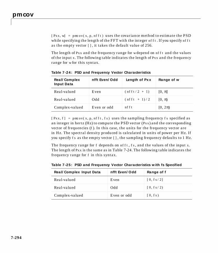
pmcov
7-294
[Pxx,w] = pmcov(x,p,nfft) uses the covariance method to estimate the PSDwhile specifying the length of the FFT with the integer nfft. If you specify nfftas the empty vector [], it takes the default value of 256.
The length of Pxx and the frequency range for w depend on nfft and the valuesof the input x. The following table indicates the length of Pxx and the frequencyrange for w for this syntax.
[Pxx,f] = pmcov(x,p,nfft,fs) uses the sampling frequency fs specified asan integer in hertz (Hz) to compute the PSD vector (Pxx) and the correspondingvector of frequencies (f). In this case, the units for the frequency vector arein Hz. The spectral density produced is calculated in units of power per Hz. Ifyou specify fs as the empty vector [], the sampling frequency defaults to 1 Hz.
The frequency range for f depends on nfft, fs, and the values of the input x.The length of Pxx is the same as in Table 7-24. The following table indicates thefrequency range for f in this syntax.
Table 7-24: PSD and Frequency Vector Characteristics
Real/Complex Input Data
nfft Even/Odd Length of Pxx Range of w
Real-valued Even (nfft/2 + 1) [0, π]
Real-valued Odd (nfft + 1)/2 [0, π)
Complex-valued Even or odd nfft [0, 2π)
Table 7-25: PSD and Frequency Vector Characteristics with fs Specified
Real/Complex Input Data nfft Even/Odd Range of f
Real-valued Even [0,fs/2]
Real-valued Odd [0,fs/2)
Complex-valued Even or odd [0,fs)
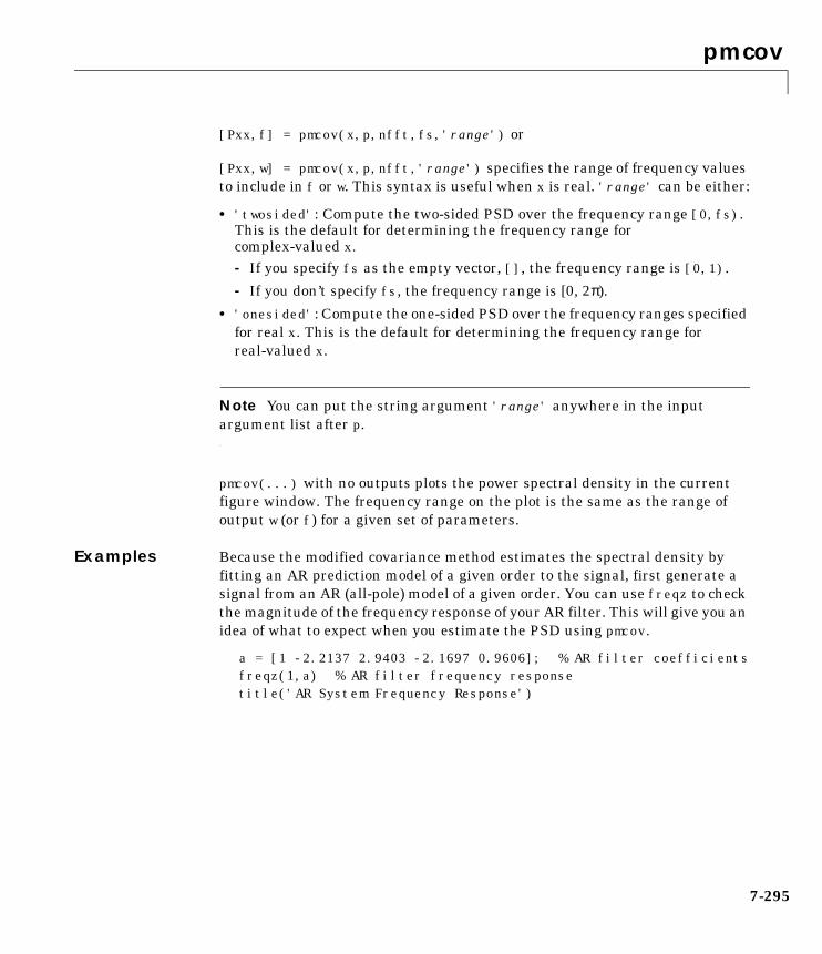
pmcov
7-295
[Pxx,f] = pmcov(x,p,nfft,fs,'range') or
[Pxx,w] = pmcov(x,p,nfft,'range') specifies the range of frequency valuesto include in f or w. This syntax is useful when x is real. 'range' can be either:
• 'twosided': Compute the two-sided PSD over the frequency range [0,fs).This is the default for determining the frequency range forcomplex-valued x.
- If you specify fs as the empty vector, [], the frequency range is [0,1).
- If you don’t specify fs, the frequency range is [0, 2π).
• 'onesided': Compute the one-sided PSD over the frequency ranges specifiedfor real x. This is the default for determining the frequency range forreal-valued x.
Note You can put the string argument 'range' anywhere in the inputargument list after p.
pmcov(...) with no outputs plots the power spectral density in the currentfigure window. The frequency range on the plot is the same as the range ofoutput w (or f) for a given set of parameters.
Examples Because the modified covariance method estimates the spectral density byfitting an AR prediction model of a given order to the signal, first generate asignal from an AR (all-pole) model of a given order. You can use freqz to checkthe magnitude of the frequency response of your AR filter. This will give you anidea of what to expect when you estimate the PSD using pmcov.
a = [1 -2.2137 2.9403 -2.1697 0.9606]; % AR filter coefficientsfreqz(1,a) % AR filter frequency responsetitle('AR System Frequency Response')

pmcov
7-296
Now generate the input signal x by filtering white noise through the AR filter.Estimate the PSD of x based on a fourth-order AR prediction model since in thiscase we know that the original AR system model a has order 4.
randn('state',1);x = filter(1,a,randn(256,1)); % AR filter outputpmcov(x,4) % Fourth-order estimate
0 0.1 0.2 0.3 0.4 0.5 0.6 0.7 0.8 0.9 1−200
−150
−100
−50
0
50
100
Normalized Frequency (×π rad/sample)
Pha
se (
degr
ees)
0 0.1 0.2 0.3 0.4 0.5 0.6 0.7 0.8 0.9 1−20
−10
0
10
20
30
40
Normalized Frequency (×π rad/sample)
Mag
nitu
de (
dB)
AR System Frequency Response
0 0.1 0.2 0.3 0.4 0.5 0.6 0.7 0.8 0.9 1−30
−20
−10
0
10
20
30
Normalized Frequency (×π rad/sample)
Pow
er S
pect
ral D
ensi
ty (
dB/ r
ad/s
ampl
e)
Modified Covariance PSD Estimate

pmcov
7-297
Remarks The power spectral density is computed as the distribution of power per unitfrequency.
This algorithm depends on your selecting an appropriate model order for yoursignal.
Algorithm Linear prediction filters can be used to model the second-order statisticalcharacteristics of a signal. The prediction filter output can be used to model thesignal when the input is white noise.
pmcov estimates the PSD of the signal vector using the modified covariancemethod. This method fits an autoregressive (AR) linear prediction filter modelto the signal by simultaneously minimizing the forward and backwardprediction errors (based on causal observations of your input signal) in theleast squares sense. The spectral estimate returned by pmcov is the magnitudesquared frequency response of this AR model.
pmcov
7-298
See Also
References [1] Marple, S.L. Digital Spectral Analysis, Englewood Cliffs, NJ, Prentice-Hall,1987, Chapter 7.
[2] Stoica, P., and R.L. Moses, Introduction to Spectral Analysis, Prentice-Hall,1997.
armcov Compute an estimate of AR model parameters usingthe modified covariance method.
lpc Linear prediction coefficients.
pburg Estimate the power spectral density using the Burgmethod.
pcov Estimate the power spectral density using thecovariance method.
peig Estimate the pseudospectrum using the eigenvectormethod.
periodogram Estimate the power spectral density using aperiodogram.
pmtm Estimate the power spectral density using themultitaper method.
pmusic Estimate the pseudospectrum using the MUSICalgorithm.
prony Prony’s method for time domain IIR filter design.
psdplot Plot power spectral density data.
pwelch Estimate the power spectral density using Welch’smethod.
pyulear Estimate the power spectral density using theYule-Walker AR method.
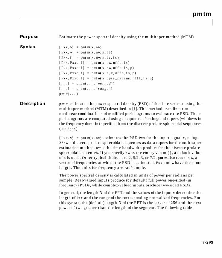
pmtm
7-299
7pmtmPurpose Estimate the power spectral density using the multitaper method (MTM).
Syntax [Pxx,w] = pmtm(x,nw)[Pxx,w] = pmtm(x,nw,nfft)[Pxx,f] = pmtm(x,nw,nfft,fs)[Pxx,Pxxc,f] = pmtm(x,nw,nfft,fs)[Pxx,Pxxc,f] = pmtm(x,nw,nfft,fs,p)[Pxx,Pxxc,f] = pmtm(x,e,v,nfft,fs,p)[Pxx,Pxxc,f] = pmtm(x,dpss_params,nfft,fs,p)[...] = pmtm(...,'method')[...] = pmtm(...,'range')pmtm(...)
Description pmtm estimates the power spectral density (PSD) of the time series x using themultitaper method (MTM) described in [1]. This method uses linear ornonlinear combinations of modified periodograms to estimate the PSD. Theseperiodograms are computed using a sequence of orthogonal tapers (windows inthe frequency domain) specified from the discrete prolate spheroidal sequences(see dpss).
[Pxx,w] = pmtm(x,nw) estimates the PSD Pxx for the input signal x, using2*nw-1 discrete prolate spheroidal sequences as data tapers for the multitaperestimation method. nw is the time-bandwidth product for the discrete prolatespheroidal sequences. If you specify nw as the empty vector [], a default valueof 4 is used. Other typical choices are 2, 5/2, 3, or 7/2. pmtm also returns w, avector of frequencies at which the PSD is estimated. Pxx and w have the samelength. The units for frequency are rad/sample.
The power spectral density is calculated in units of power per radians persample. Real-valued inputs produce (by default) full power one-sided (infrequency) PSDs, while complex-valued inputs produce two-sided PSDs.
In general, the length N of the FFT and the values of the input x determine thelength of Pxx and the range of the corresponding normalized frequencies. Forthis syntax, the (default) length N of the FFT is the larger of 256 and the nextpower of two greater than the length of the segment. The following table
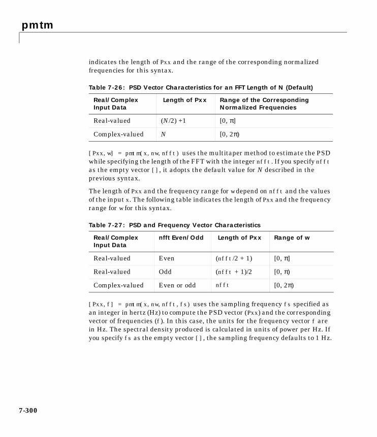
pmtm
7-300
indicates the length of Pxx and the range of the corresponding normalizedfrequencies for this syntax.
[Pxx,w] = pmtm(x,nw,nfft) uses the multitaper method to estimate the PSDwhile specifying the length of the FFT with the integer nfft. If you specify nfftas the empty vector [], it adopts the default value for N described in theprevious syntax.
The length of Pxx and the frequency range for w depend on nfft and the valuesof the input x. The following table indicates the length of Pxx and the frequencyrange for w for this syntax.
[Pxx,f] = pmtm(x,nw,nfft,fs) uses the sampling frequency fs specified asan integer in hertz (Hz) to compute the PSD vector (Pxx) and the correspondingvector of frequencies (f). In this case, the units for the frequency vector f arein Hz. The spectral density produced is calculated in units of power per Hz. Ifyou specify fs as the empty vector [], the sampling frequency defaults to 1 Hz.
Table 7-26: PSD Vector Characteristics for an FFT Length of N (Default)
Real/Complex Input Data
Length of Pxx Range of the Corresponding Normalized Frequencies
Real-valued (N/2) +1 [0, π]
Complex-valued N [0, 2π)
Table 7-27: PSD and Frequency Vector Characteristics
Real/Complex Input Data
nfft Even/Odd Length of Pxx Range of w
Real-valued Even (nfft/2 + 1) [0, π]
Real-valued Odd (nfft + 1)/2 [0, π)
Complex-valued Even or odd nfft [0, 2π)
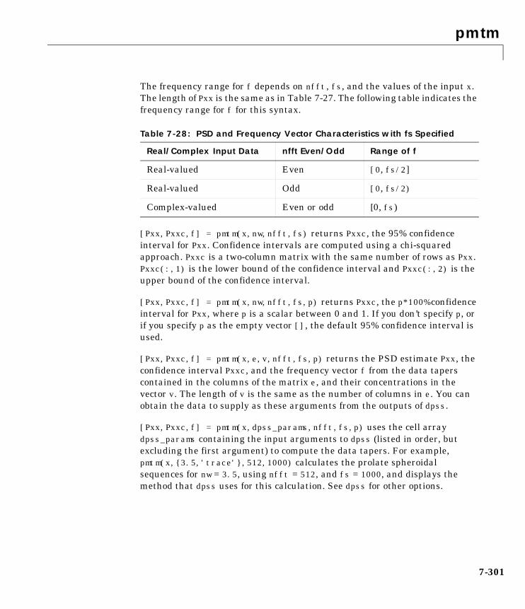
pmtm
7-301
The frequency range for f depends on nfft, fs, and the values of the input x.The length of Pxx is the same as in Table 7-27. The following table indicates thefrequency range for f for this syntax.
[Pxx,Pxxc,f] = pmtm(x,nw,nfft,fs) returns Pxxc, the 95% confidenceinterval for Pxx. Confidence intervals are computed using a chi-squaredapproach. Pxxc is a two-column matrix with the same number of rows as Pxx.Pxxc(:,1) is the lower bound of the confidence interval and Pxxc(:,2) is theupper bound of the confidence interval.
[Pxx,Pxxc,f] = pmtm(x,nw,nfft,fs,p) returns Pxxc, the p*100% confidenceinterval for Pxx, where p is a scalar between 0 and 1. If you don’t specify p, orif you specify p as the empty vector [], the default 95% confidence interval isused.
[Pxx,Pxxc,f] = pmtm(x,e,v,nfft,fs,p) returns the PSD estimate Pxx, theconfidence interval Pxxc, and the frequency vector f from the data taperscontained in the columns of the matrix e, and their concentrations in thevector v. The length of v is the same as the number of columns in e. You canobtain the data to supply as these arguments from the outputs of dpss.
[Pxx,Pxxc,f] = pmtm(x,dpss_params,nfft,fs,p) uses the cell arraydpss_params containing the input arguments to dpss (listed in order, butexcluding the first argument) to compute the data tapers. For example,pmtm(x,3.5,'trace',512,1000) calculates the prolate spheroidalsequences for nw = 3.5, using nfft = 512, and fs = 1000, and displays themethod that dpss uses for this calculation. See dpss for other options.
Table 7-28: PSD and Frequency Vector Characteristics with fs Specified
Real/Complex Input Data nfft Even/Odd Range of f
Real-valued Even [0, fs/2]
Real-valued Odd [0, fs/2)
Complex-valued Even or odd [0, fs)

pmtm
7-302
[...] = pmtm(...,'method') specifies the algorithm used for combining theindividual spectral estimates. The string 'method' can be one of the following:
• 'adapt': Thomson’s adaptive nonlinear combination (default)
• 'unity': A linear combination of the weighted periodograms with unityweights
• 'eigen': A linear combination of the weighted periodograms witheigenvalue weights
[...] = pmtm(...,'range') specifies the range of frequency values to includein f or w. This syntax is useful when x is real. 'range' can be either:
• 'twosided': Compute the two-sided PSD over the frequency range [0,fs).This is the default for determining the frequency range for complex-valuedx.
- If you specify fs as the empty vector, [], the frequency range is [0,1).
- If you don’t specify fs, the frequency range is [0, 2π).
• 'onesided': Compute the one-sided PSD over the frequency ranges specifiedfor real x. This is the default for determining the frequency range forreal-valued x.
Note You can put the string arguments 'range' or 'method' anywhere afterthe input argument nw or v.
pmtm(...) with no output arguments plots the PSD estimate and theconfidence intervals in the current figure window. If you don’t specify fs, the95% confidence interval is plotted. If you do specify fs, the confidence intervalsplotted depend on the value of p.
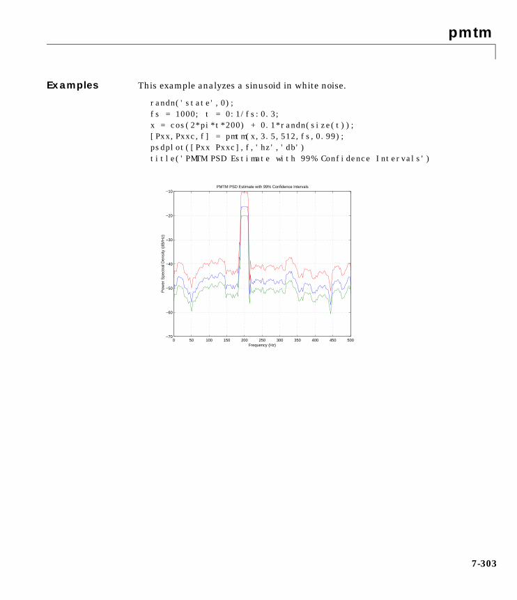
pmtm
7-303
Examples This example analyzes a sinusoid in white noise.
randn('state',0);fs = 1000; t = 0:1/fs:0.3;x = cos(2*pi*t*200) + 0.1*randn(size(t));[Pxx,Pxxc,f] = pmtm(x,3.5,512,fs,0.99);psdplot([Pxx Pxxc],f,'hz','db')title('PMTM PSD Estimate with 99% Confidence Intervals')
0 50 100 150 200 250 300 350 400 450 500−70
−60
−50
−40
−30
−20
−10
Frequency (Hz)
Po
we
r S
pe
ctra
l De
nsi
ty (
dB
/Hz)
PMTM PSD Estimate with 99% Confidence Intervals

pmtm
7-304
See Also
References [1] Percival, D.B., and A.T. Walden, Spectral Analysis for PhysicalApplications: Multitaper and Conventional Univariate Techniques, CambridgeUniversity Press, 1993.
[2] Thomson, D.J., “Spectrum estimation and harmonic analysis,” Proceedingsof the IEEE, Vol. 70 (1982), pp. 1055-1096.
dpss Compute the discrete prolate spheroidal sequences(Slepian sequences).
pburg Estimate the power spectral density using the Burgmethod.
pcov Estimate the power spectral density using thecovariance method.
peig Estimate the pseudospectrum using the eigenvectormethod.
periodogram Estimate the power spectral density using aperiodogram.
pmcov Estimate the power spectral density using themodified covariance method.
pmusic Estimate the pseudospectrum using the MUSICalgorithm.
psdplot Plot power spectral density data.
pwelch Estimate the power spectral density using Welch’smethod.
pyulear Estimate the power spectral density using theYule-Walker AR method.
pmusic
7-305
7pmusicPurpose Estimate the pseudospectrum using the MUSIC algorithm.
Syntax [S,w] = pmusic(x,p)[S,w] = pmusic(...,nfft)[S,f] = pmusic(x,p,nfft,fs))[S,f] = pmusic(...,'corr')[S,f] = pmusic(x,p,nfft,fs,nwin,noverlap)[...] = pmusic(...,'range')[...,v,e] = pmusic(...)pmusic(...)
Description [S,w] = pmusic(x,p) implements the MUSIC (Multiple Signal Classification)algorithm and returns S, the pseudospectrum estimate of the input signal x,and a vector w of normalized frequencies (in rad/sample) at which thepseudospectrum is evaluated. The pseudospectrum is calculated usingestimates of the eigenvectors of a correlation matrix associated with the inputdata x, where x is specified as either:
• A row or column vector representing one observation of the signal
• A rectangular array for which each row of x represents a separateobservation of the signal (for example, each row is one output of an array ofsensors, as in array processing), such that x'*x is an estimate of thecorrelation matrix
Note You can use the output of corrmtx to generate such an array x.
You can specify the second input argument p as either:
• A scalar integer. In this case, the signal subspace dimension is p.
• A two-element vector. In this case, p(2), the second element of p, representsa threshold that is multiplied by λmin, the smallest estimated eigenvalue ofthe signal’s correlation matrix. Eigenvalues below the threshold λmin*p(2)are assigned to the noise subspace. In this case, p(1) specifies the maximumdimension of the signal subspace.

pmusic
7-306
The extra threshold parameter in the second entry in p provides you moreflexibility and control in assigning the noise and signal subspaces.
S and w have the same length. In general, the length of the FFT and the valuesof the input x determine the length of the computed S and the range of thecorresponding normalized frequencies. The following table indicates the lengthof S (and w) and the range of the corresponding normalized frequencies for thissyntax.
[S,w] = pmusic(...,nfft) specifies the length of the FFT used to estimatethe pseudospectrum with the integer nfft. The default value for nfft (enteredas an empty vector []) is 256.
The following table indicates the length of S and w, and the frequency range forw in this syntax.
[S,f] = pmusic(x,p,nfft,fs) returns the pseudospectrum in the vector Sevaluated at the corresponding vector of frequencies f (in Hz). You supply thesampling frequency fs in Hz. If you specify fs with the empty vector [], thesampling frequency defaults to 1 Hz.
Table 7-29: S Characteristics for an FFT Length of 256 (Default)
Real/Complex Input Data
Length of S and w Range of the Corresponding Normalized Frequencies
Real-valued 129 [0, π]
Complex-valued 256 [0, 2π)
Table 7-30: S and Frequency Vector Characteristics
Real/Complex Input Data
nfft Even/Odd Length of S and w
Range of w
Real-valued Even (nfft/2 + 1) [0, π]
Real-valued Odd (nfft + 1)/2 [0, π)
Complex-valued Even or odd nfft [0, 2π)
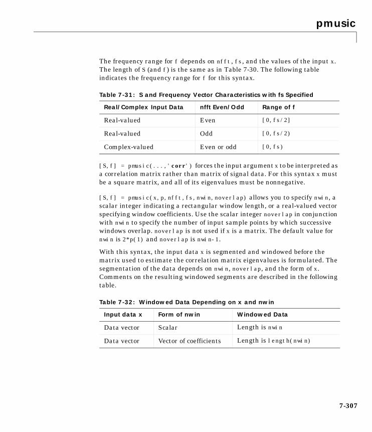
pmusic
7-307
The frequency range for f depends on nfft, fs, and the values of the input x.The length of S (and f) is the same as in Table 7-30. The following tableindicates the frequency range for f for this syntax.
[S,f] = pmusic(...,'corr') forces the input argument x to be interpreted asa correlation matrix rather than matrix of signal data. For this syntax x mustbe a square matrix, and all of its eigenvalues must be nonnegative.
[S,f] = pmusic(x,p,nfft,fs,nwin,noverlap) allows you to specify nwin, ascalar integer indicating a rectangular window length, or a real-valued vectorspecifying window coefficients. Use the scalar integer noverlap in conjunctionwith nwin to specify the number of input sample points by which successivewindows overlap. noverlap is not used if x is a matrix. The default value fornwin is 2*p(1) and noverlap is nwin-1.
With this syntax, the input data x is segmented and windowed before thematrix used to estimate the correlation matrix eigenvalues is formulated. Thesegmentation of the data depends on nwin, noverlap, and the form of x.Comments on the resulting windowed segments are described in the followingtable.
Table 7-31: S and Frequency Vector Characteristics with fs Specified
Real/Complex Input Data nfft Even/Odd Range of f
Real-valued Even [0,fs/2]
Real-valued Odd [0,fs/2)
Complex-valued Even or odd [0,fs)
Table 7-32: Windowed Data Depending on x and nwin
Input data x Form of nwin Windowed Data
Data vector Scalar Length is nwin
Data vector Vector of coefficients Length is length(nwin)
pmusic
7-308
See Table 7-33 for related information on this syntax.
Note The arguments nwin and noverlap are ignored when you include thestring 'corr' in the syntax.
[...] = pmusic(...,'range') specifies the range of frequency values toinclude in f or w. This syntax is useful when x is real. 'range' can be either:
• 'whole': Compute the pseudospectrum over the frequency range [0,fs).This is the default for determining the frequency range for complex-valued x. - If you specify fs as the empty vector, [], the frequency range is [0,1).
- If you don’t specify fs, the frequency range is [0, 2π).
• 'half': Compute the pseudospectrum over the frequency ranges specifiedfor real x. This is the default for determining the frequency range forreal-valued x.
Note You can put the string arguments 'range' or 'corr' anywhere in theinput argument list after p.
[...,v,e] = pmusic(...) returns the matrix v of noise eigenvectors, alongwith the associated eigenvalues in the vector e. The columns of v span the noisesubspace of dimension size(v,2). The dimension of the signal subspace issize(v,1)-size(v,2). For this syntax, e is a vector of estimated eigenvaluesof the correlation matrix.
Data matrix Scalar Data is not windowed.
Data matrix Vector of coefficients length(nwin) must be thesame as the column length of x,and noverlap is not used.
Table 7-32: Windowed Data Depending on x and nwin (Continued)
Input data x Form of nwin Windowed Data

pmusic
7-309
pmusic(...) with no output arguments plots the pseudospectrum in thecurrent figure window.
Remarks In the process of estimating the pseudospectrum, pmusic computes the noiseand signal subspaces from the estimated eigenvectors vj and eigenvalues λj ofthe signal’s correlation matrix. The smallest of these eigenvalues is used inconjunction with the threshold parameter p(2) to affect the dimension of thenoise subspace in some cases.
The length n of the eigenvectors computed by pmusic is the sum of thedimensions of the signal and noise subspaces. This eigenvector length dependson your input (signal data or correlation matrix) and the syntax you use.
The following table summarizes the dependency of the eigenvector length onthe input argument.
You should specify nwin > p(1) or length(nwin) > p(1) if you want p(2) > 1 tohave any effect.
Table 7-33: Eigenvector Length Depending on Input Data and Syntax
Form of Input Data x Comments on the Syntax Length n of Eigenvectors
Row or column vector nwin is specified as a scalarinteger.
nwin
Row or column vector nwin is specified as a vector. length(nwin)
Row or column vector nwin is not specified. 2*p(1)
l-by-m matrix If nwin is specified as ascalar, it is not used. If nwinis specified as a vector,length(nwin) must equalm.
m
m-by-m nonnegativedefinite matrix
The string 'corr' isspecified and nwin is notused.
m
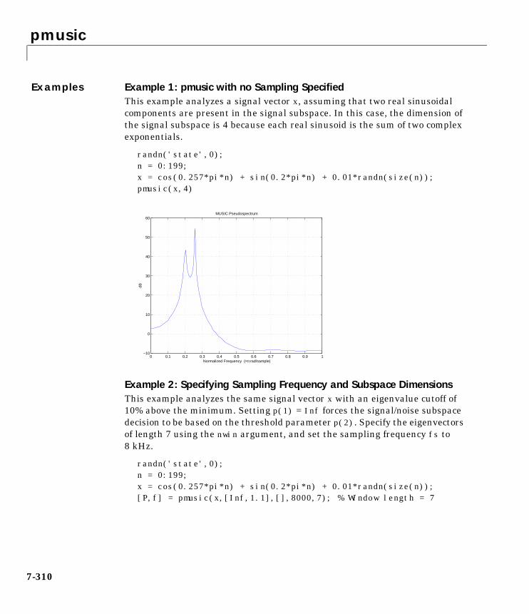
pmusic
7-310
Examples Example 1: pmusic with no Sampling SpecifiedThis example analyzes a signal vector x, assuming that two real sinusoidalcomponents are present in the signal subspace. In this case, the dimension ofthe signal subspace is 4 because each real sinusoid is the sum of two complexexponentials.
randn('state',0);n = 0:199;x = cos(0.257*pi*n) + sin(0.2*pi*n) + 0.01*randn(size(n));pmusic(x,4)
Example 2: Specifying Sampling Frequency and Subspace DimensionsThis example analyzes the same signal vector x with an eigenvalue cutoff of10% above the minimum. Setting p(1) = Inf forces the signal/noise subspacedecision to be based on the threshold parameter p(2). Specify the eigenvectorsof length 7 using the nwin argument, and set the sampling frequency fs to8 kHz.
randn('state',0);n = 0:199;x = cos(0.257*pi*n) + sin(0.2*pi*n) + 0.01*randn(size(n));[P,f] = pmusic(x,[Inf,1.1],[],8000,7); % Window length = 7
0 0.1 0.2 0.3 0.4 0.5 0.6 0.7 0.8 0.9 1−10
0
10
20
30
40
50
60
Normalized Frequency (×π rad/sample)
dB
MUSIC Pseudospectrum
pmusic
7-311
Example 3: Entering a Correlation MatrixSupply a positive definite correlation matrix R for estimating the spectraldensity. Use the default 256 samples.
R = toeplitz(cos(0.1*pi*[0:6])) + 0.1*eye(7);[P,f] = pmusic(R,4,'corr');
Example 4: Entering a Signal Data Matrix Generated from corrmtxEnter a signal data matrix Xm generated from data using corrmtx.
randn('state',0);n = 0:699;x = cos(0.257*pi*(n)) + 0.1*randn(size(n));Xm = corrmtx(x,7,'mod');[P,w] = pmusic(Xm,2);
Example 5: Using Windowing to Create the Effect of a Signal Data MatrixUse the same signal, but let pmusic form the 100-by-7 data matrix using itswindowing input arguments. In addition, specify an FFT of length 512.
randn('state',0);n = 0:699;x = cos(0.257*pi*(n)) + 0.1*randn(size(n));[PP,ff] = pmusic(x,2,512,[],7,0);
Algorithm The name MUSIC is an acronym for MUltiple SIgnal Classification. TheMUSIC algorithm estimates the pseudospectrum from a signal or a correlationmatrix using Schmidt’s eigenspace analysis method [1]. The algorithmperforms eigenspace analysis of the signal’s correlation matrix in order toestimate the signal’s frequency content. This algorithm is particularly suitablefor signals that are the sum of sinusoids with additive white Gaussian noise.The eigenvalues and eigenvectors of the signal’s correlation matrix areestimated if you don’t supply the correlation matrix.
The MUSIC pseudospectrum estimate is given by
Pmusicf( )1
eH f( ) vkvkH
k p 1+=
N
e f( )
---------------------------------------------------------------- 1
vkHe f( ) 2
k p 1+=
N
-------------------------------------------= =
pmusic
7-312
where N is the dimension of the eigenvectors and vk is the k-th eigenvector ofthe correlation matrix. The integer p is the dimension of the signal subspace,so the eigenvectors vk used in the sum correspond to the smallest eigenvaluesand also span the noise subspace. The vector e(f) consists of complexexponentials, so the inner product
amounts to a Fourier transform. This is used for computation of thepseudospectrum estimate. The FFT is computed for each vk and then thesquared magnitudes are summed.
See Also
References [1] Marple, S.L. Digital Spectral Analysis, Englewood Cliffs, NJ, Prentice-Hall,1987, pp. 373-378.
[2] Schmidt, R.O, “Multiple Emitter Location and Signal ParameterEstimation,” IEEE Trans. Antennas Propagation, Vol. AP-34 (March 1986),pp. 276-280.
vkHe f( )
corrmtx Prepare input data for a correlation matrix estimate.
pburg Estimate the power spectral density using the Burgmethod.
peig Estimate the pseudospectrum using the eigenvectormethod.
periodogram Estimate the power spectral density using aperiodogram.
pmtm Estimate the power spectral density using themultitaper method.
prony Prony’s method for time domain IIR filter design.
psdplot Plot power spectral density data.
pwelch Estimate the power spectral density using Welch’smethod.
rooteig Estimate the frequency and power content using theroot eigenvector method.
rootmusic Estimate the frequency and power content using theroot MUSIC algorithm.

pmusic
7-313
[3] Stoica, P., and R.L. Moses, Introduction to Spectral Analysis, Prentice-Hall,Englewood Cliffs, NJ, 1997.
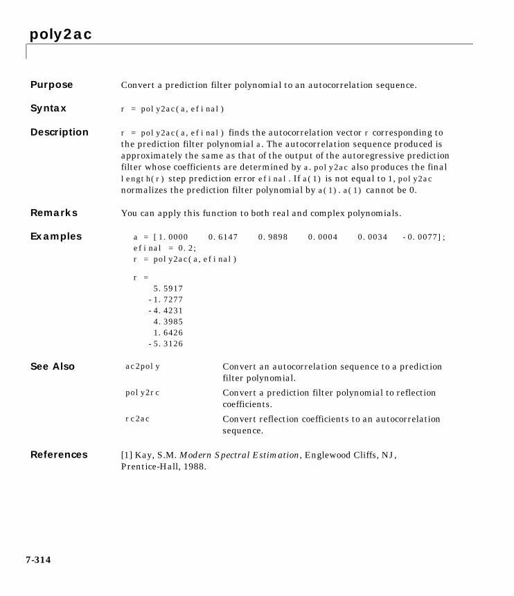
poly2ac
7-314
7poly2acPurpose Convert a prediction filter polynomial to an autocorrelation sequence.
Syntax r = poly2ac(a,efinal)
Description r = poly2ac(a,efinal) finds the autocorrelation vector r corresponding tothe prediction filter polynomial a. The autocorrelation sequence produced isapproximately the same as that of the output of the autoregressive predictionfilter whose coefficients are determined by a. poly2ac also produces the finallength(r) step prediction error efinal. If a(1) is not equal to 1, poly2acnormalizes the prediction filter polynomial by a(1). a(1) cannot be 0.
Remarks You can apply this function to both real and complex polynomials.
Examples a = [1.0000 0.6147 0.9898 0.0004 0.0034 -0.0077];efinal = 0.2;r = poly2ac(a,efinal)
r = 5.5917 -1.7277 -4.4231 4.3985 1.6426 -5.3126
See Also
References [1] Kay, S.M. Modern Spectral Estimation, Englewood Cliffs, NJ,Prentice-Hall, 1988.
ac2poly Convert an autocorrelation sequence to a predictionfilter polynomial.
poly2rc Convert a prediction filter polynomial to reflectioncoefficients.
rc2ac Convert reflection coefficients to an autocorrelationsequence.
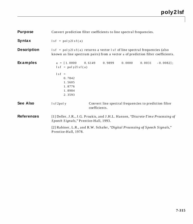
poly2lsf
7-315
7poly2lsfPurpose Convert prediction filter coefficients to line spectral frequencies.
Syntax lsf = poly2lsf(a)
Description lsf = poly2lsf(a) returns a vector lsf of line spectral frequencies (alsoknown as line spectrum pairs) from a vector a of prediction filter coefficients.
Examples a = [1.0000 0.6149 0.9899 0.0000 0.0031 -0.0082];lsf = poly2lsf(a)
lsf = 0.7842 1.5605 1.8776 1.8984 2.3593
See Also lsf2poly Convert line spectral frequencies to prediction filtercoefficients.
References [1] Deller, J.R., J.G. Proakis, and J.H.L. Hansen, “Discrete-Time Processing ofSpeech Signals,” Prentice-Hall, 1993.
[2] Rabiner, L.R., and R.W. Schafer, “Digital Processing of Speech Signals,”Prentice-Hall, 1978.
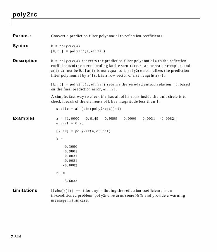
poly2rc
7-316
7poly2rcPurpose Convert a prediction filter polynomial to reflection coefficients.
Syntax k = poly2rc(a)[k,r0] = poly2rc(a,efinal)
Description k = poly2rc(a) converts the prediction filter polynomial a to the reflectioncoefficients of the corresponding lattice structure. a can be real or complex, anda(1) cannot be 0. If a(1) is not equal to 1, poly2rc normalizes the predictionfilter polynomial by a(1). k is a row vector of size length(a)-1.
[k,r0] = poly2rc(a,efinal) returns the zero-lag autocorrelation, r0, basedon the final prediction error, efinal.
A simple, fast way to check if a has all of its roots inside the unit circle is tocheck if each of the elements of k has magnitude less than 1.
stable = all(abs(poly2rc(a))<1)
Examples a = [1.0000 0.6149 0.9899 0.0000 0.0031 -0.0082];efinal = 0.2;
[k,r0] = poly2rc(a,efinal)
k =
0.3090 0.9801 0.0031 0.0081 -0.0082
r0 =
5.6032
Limitations If abs(k(i)) == 1 for any i, finding the reflection coefficients is anill-conditioned problem. poly2rc returns some NaNs and provide a warningmessage in this case.
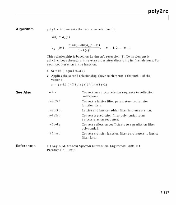
poly2rc
7-317
Algorithm poly2rc implements the recursive relationship
This relationship is based on Levinson’s recursion [1]. To implement it,poly2rc loops through a in reverse order after discarding its first element. Foreach loop iteration i, the function:
1 Sets k(i) equal to a(i)
2 Applies the second relationship above to elements 1 through i of thevector a.a = (a–k(i)*fliplr(a))/(1–k(i)^2);
See Also
References [1] Kay, S.M. Modern Spectral Estimation, Englewood Cliffs, NJ,Prentice-Hall, 1988.
k n( ) an n( )=
an 1– m( )an m( ) k n( )an n m–( )–
1 k n( )2–---------------------------------------------------------- m 1= 2 … n 1–, , , ,=
ac2rc Convert an autocorrelation sequence to reflectioncoefficients.
latc2tf Convert a lattice filter parameters to transferfunction form.
latcfilt Lattice and lattice-ladder filter implementation.
poly2ac Convert a prediction filter polynomial to anautocorrelation sequence.
rc2poly Convert reflection coefficients to a prediction filterpolynomial.
tf2latc Convert transfer function filter parameters to latticefilter form.

polyscale
7-318
7polyscalePurpose Scale the roots of a polynomial.
Syntax b = polyscale(a,alpha)
Description b = polyscale(a,alpha) scales the roots of a polynomial in the z-plane,where a is a vector containing the polynomial coefficients and alpha is thescaling factor.
If alpha is a real value in the range [0 1], then the roots of a are radially scaledtoward the origin in the z-plane. Complex values for alpha allow arbitrarychanges to the root locations.
Remark By reducing the radius of the roots in an autoregressive polynomial, thebandwidth of the spectral peaks in the frequency response is expanded(flattened). This operation is often referred to as bandwidth expansion.
See Also polystab Stabilize a polynomial.
roots Polynomial roots (see the MATLAB documentation).

polystab
7-319
7polystabPurpose Stabilize polynomial.
Syntax b = polystab(a)
Description polystab stabilizes a polynomial with respect to the unit circle; it reflects rootswith magnitudes greater than 1 inside the unit circle.
b = polystab(a) returns a row vector b containing the stabilized polynomial,where a is a vector of polynomial coefficients, normally in the z-domain.
Examples polystab can convert a linear-phase filter into a minimum-phase filter withthe same magnitude response.
h = fir1(25,0.4);hmin = polystab(h) * norm(h)/norm(polystab(h));
Algorithm polystab finds the roots of the polynomial and maps those roots found outsidethe unit circle to the inside of the unit circle.
v = roots(a);vs = 0.5*(sign(abs(v)-1)+1);v = (1-vs).*v + vs./conj(v);b = a(1)*poly(v);
See Also
a z( ) a 1( ) a 2( )z 1– a na 1+( )z na–+ + +=
roots Polynomial roots (see the MATLAB documentation).
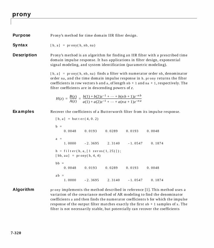
prony
7-320
7pronyPurpose Prony’s method for time domain IIR filter design.
Syntax [b,a] = prony(h,nb,na)
Description Prony’s method is an algorithm for finding an IIR filter with a prescribed timedomain impulse response. It has applications in filter design, exponentialsignal modeling, and system identification (parametric modeling).
[b,a] = prony(h,nb,na) finds a filter with numerator order nb, denominatororder na, and the time domain impulse response in h. prony returns the filtercoefficients in row vectors b and a, of length nb + 1 and na + 1, respectively. Thefilter coefficients are in descending powers of z.
Examples Recover the coefficients of a Butterworth filter from its impulse response.
[b,a] = butter(4,0.2)
b =0.0048 0.0193 0.0289 0.0193 0.0048
a =1.0000 -2.3695 2.3140 -1.0547 0.1874
h = filter(b,a,[1 zeros(1,25)]);[bb,aa] = prony(h,4,4)
bb =0.0048 0.0193 0.0289 0.0193 0.0048
ab =1.0000 -2.3695 2.3140 -1.0547 0.1874
Algorithm prony implements the method described in reference [1]. This method uses avariation of the covariance method of AR modeling to find the denominatorcoefficients a and then finds the numerator coefficients b for which the impulseresponse of the output filter matches exactly the first nb + 1 samples of x. Thefilter is not necessarily stable, but potentially can recover the coefficients
H z( )B z( )A z( )----------- b 1( ) b 2( )z 1– b nb 1+( )z nb–+ + +
a 1( ) a 2( )z 1– a na 1+( )z na–+ + +--------------------------------------------------------------------------------------------= =

prony
7-321
exactly if the data sequence is truly an autoregressive moving average (ARMA)process of the correct order.
See Also
References [1] Parks, T.W., and C.S. Burrus, Digital Filter Design, John Wiley & Sons,1987, pp. 226-228.
butter Butterworth analog and digital filter design.
cheby1 Chebyshev type I filter design (passband ripple).
cheby2 Chebyshev type II filter design (stopband ripple).
ellip Elliptic (Cauer) filter design.
invfreqz Identify discrete-time filter parameters fromfrequency response data.
levinson Compute the Levinson-Durbin recursion.
lpc Compute linear prediction filter coefficients.
stmcb Compute a linear model using Steiglitz-McBrideiteration.
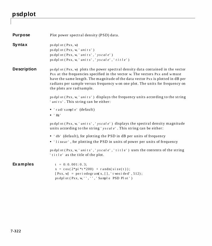
psdplot
7-322
7psdplotPurpose Plot power spectral density (PSD) data.
Syntax psdplot(Pxx,w)psdplot(Pxx,w,'units')psdplot(Pxx,w,'units','yscale')psdplot(Pxx,w,'units','yscale','title')
Description psdplot(Pxx,w) plots the power spectral density data contained in the vectorPxx at the frequencies specified in the vector w. The vectors Pxx and w musthave the same length. The magnitude of the data vector Pxx is plotted in dB perradians per sample versus frequency w on one plot. The units for frequency onthe plots are rad/sample.
psdplot(Pxx,w,'units') displays the frequency units according to the string'units'. This string can be either:
• 'rad/sample' (default)• 'Hz'
psdplot(Pxx,w,'units','yscale') displays the spectral density magnitudeunits according to the string 'yscale'. This string can be either:
• 'db' (default), for plotting the PSD in dB per units of frequency• 'linear', for plotting the PSD in units of power per units of frequency
psdplot(Pxx,w,'units','yscale','title') uses the contents of the string'title' as the title of the plot.
Examples t = 0:0.001:0.3;x = cos(2*pi*t*200) + randn(size(t)); [Pxx,w] = periodogram(x,[],'twosided',512);psdplot(Pxx,w,'','','Sample PSD Plot')
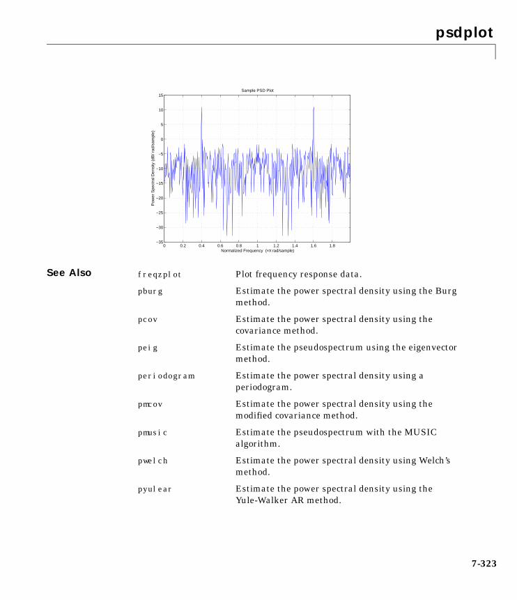
psdplot
7-323
See Also
0 0.2 0.4 0.6 0.8 1 1.2 1.4 1.6 1.8−35
−30
−25
−20
−15
−10
−5
0
5
10
15
Normalized Frequency (×π rad/sample)
Pow
er S
pect
ral D
ensi
ty (
dB/ r
ad/s
ampl
e)
Sample PSD Plot
freqzplot Plot frequency response data.
pburg Estimate the power spectral density using the Burgmethod.
pcov Estimate the power spectral density using thecovariance method.
peig Estimate the pseudospectrum using the eigenvectormethod.
periodogram Estimate the power spectral density using aperiodogram.
pmcov Estimate the power spectral density using themodified covariance method.
pmusic Estimate the pseudospectrum with the MUSICalgorithm.
pwelch Estimate the power spectral density using Welch’smethod.
pyulear Estimate the power spectral density using theYule-Walker AR method.
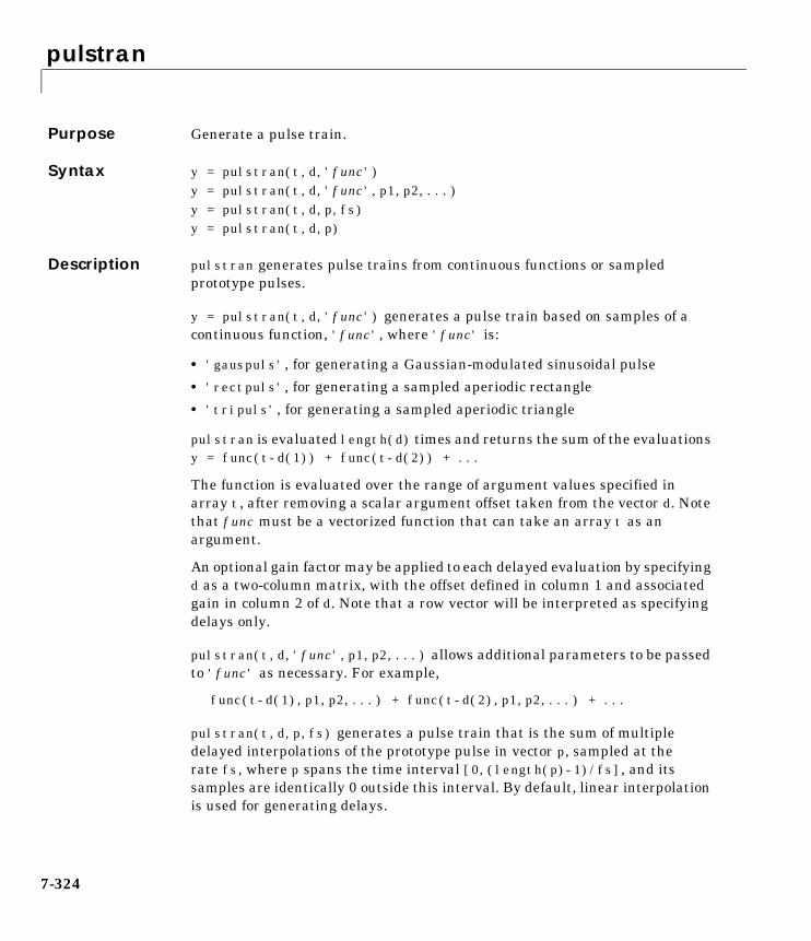
pulstran
7-324
7pulstranPurpose Generate a pulse train.
Syntax y = pulstran(t,d,'func')y = pulstran(t,d,'func',p1,p2,...)y = pulstran(t,d,p,fs)y = pulstran(t,d,p)
Description pulstran generates pulse trains from continuous functions or sampledprototype pulses.
y = pulstran(t,d,'func') generates a pulse train based on samples of acontinuous function, 'func', where 'func' is:
• 'gauspuls', for generating a Gaussian-modulated sinusoidal pulse
• 'rectpuls', for generating a sampled aperiodic rectangle
• 'tripuls', for generating a sampled aperiodic triangle
pulstran is evaluated length(d) times and returns the sum of the evaluationsy = func(t-d(1)) + func(t-d(2)) + ...
The function is evaluated over the range of argument values specified inarray t, after removing a scalar argument offset taken from the vector d. Notethat func must be a vectorized function that can take an array t as anargument.
An optional gain factor may be applied to each delayed evaluation by specifyingd as a two-column matrix, with the offset defined in column 1 and associatedgain in column 2 of d. Note that a row vector will be interpreted as specifyingdelays only.
pulstran(t,d,'func',p1,p2,...) allows additional parameters to be passedto 'func' as necessary. For example,
func(t-d(1),p1,p2,...) + func(t-d(2),p1,p2,...) + ...
pulstran(t,d,p,fs) generates a pulse train that is the sum of multipledelayed interpolations of the prototype pulse in vector p, sampled at therate fs, where p spans the time interval [0,(length(p)-1)/fs], and itssamples are identically 0 outside this interval. By default, linear interpolationis used for generating delays.
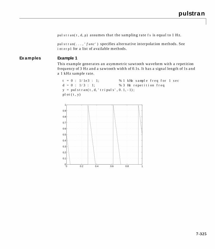
pulstran
7-325
pulstran(t,d,p) assumes that the sampling rate fs is equal to 1 Hz.
pulstran(...,'func') specifies alternative interpolation methods. Seeinterp1 for a list of available methods.
Examples Example 1This example generates an asymmetric sawtooth waveform with a repetitionfrequency of 3 Hz and a sawtooth width of 0.1s. It has a signal length of 1s anda 1 kHz sample rate.
t = 0 : 1/1e3 : 1; % 1 kHz sample freq for 1 sec d = 0 : 1/3 : 1; % 3 Hz repetition freq y = pulstran(t,d,'tripuls',0.1,-1);plot(t,y)
0 0.2 0.4 0.6 0.8 10
0.1
0.2
0.3
0.4
0.5
0.6
0.7
0.8
0.9
1
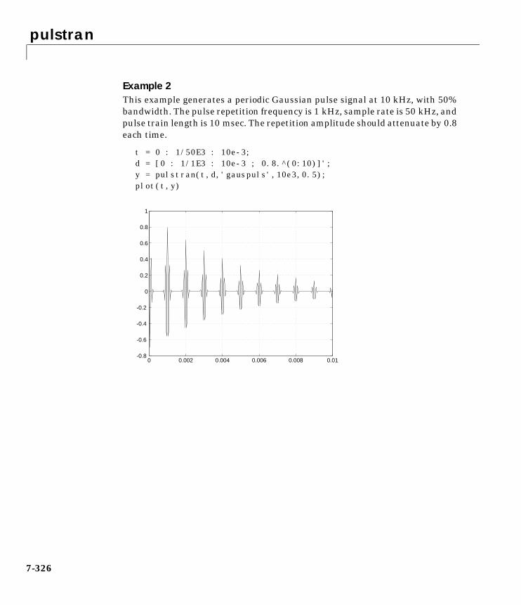
pulstran
7-326
Example 2This example generates a periodic Gaussian pulse signal at 10 kHz, with 50%bandwidth. The pulse repetition frequency is 1 kHz, sample rate is 50 kHz, andpulse train length is 10 msec. The repetition amplitude should attenuate by 0.8each time.
t = 0 : 1/50E3 : 10e-3;d = [0 : 1/1E3 : 10e-3 ; 0.8.^(0:10)]';y = pulstran(t,d,'gauspuls',10e3,0.5); plot(t,y)
0 0.002 0.004 0.006 0.008 0.01-0.8
-0.6
-0.4
-0.2
0
0.2
0.4
0.6
0.8
1
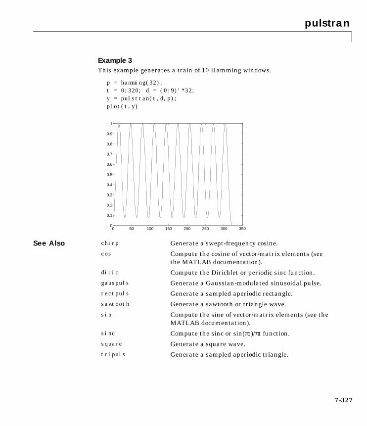
pulstran
7-327
Example 3This example generates a train of 10 Hamming windows.
p = hamming(32);t = 0:320; d = (0:9)'*32;y = pulstran(t,d,p);plot(t,y)
See Also
0 50 100 150 200 250 300 3500
0.1
0.2
0.3
0.4
0.5
0.6
0.7
0.8
0.9
1
chirp Generate a swept-frequency cosine.
cos Compute the cosine of vector/matrix elements (seethe MATLAB documentation).
diric Compute the Dirichlet or periodic sinc function.
gauspuls Generate a Gaussian-modulated sinusoidal pulse.
rectpuls Generate a sampled aperiodic rectangle.
sawtooth Generate a sawtooth or triangle wave.
sin Compute the sine of vector/matrix elements (see theMATLAB documentation).
sinc Compute the sinc or sin(πt)/πt function.
square Generate a square wave.
tripuls Generate a sampled aperiodic triangle.
pwelch
7-328
7pwelchPurpose Estimate the power spectral density (PSD) of a signal using Welch’s method.
Syntax [Pxx,w] = pwelch(x)[Pxx,w] = pwelch(x,nwin)[Pxx,w] = pwelch(x,nwin,noverlap)[Pxx,w] = pwelch(x,nwin,noverlap,nfft)[Pxx,f] = pwelch(x,nwin,noverlap,nfft,fs)[...] = pwelch(x,nwin,noverlap,...,'range')pwelch(...)
Description [Pxx,w] = pwelch(x) estimates the power spectral density Pxx of the inputsignal vector x using Welch’s averaged modified periodogram method ofspectral estimation. With this syntax:
• The vector x is segmented into eight sections of equal length, each with 50%overlap.
• Any remaining (trailing) entries in x that cannot be included in the eightsegments of equal length are discarded.
• Each segment is windowed with a Hamming window (see hamming) that isthe same length as the segment.
The power spectral density is calculated in units of power per radians persample. The corresponding vector of frequencies w is computed in radians persample, and has the same length as Pxx.
A real-valued input vector x produces a full power one-sided (in frequency) PSD(by default), while a complex-valued x produces a two-sided PSD.
In general, the length N of the FFT and the values of the input x determine thelength of Pxx and the range of the corresponding normalized frequencies. Forthis syntax, the (default) length N of the FFT is the larger of 256 and the nextpower of two greater than the length of the segment. The following table

pwelch
7-329
indicates the length of Pxx and the range of the corresponding normalizedfrequencies for this syntax.
[Pxx,w] = pwelch(x,nwin) calculates the modified periodogram using either:
• The window length nwin for the Hamming window when nwin is a positiveinteger
• The window weights specified in nwin when nwin is a vector
With this syntax, the input vector x is divided into an integer number ofsegments with 50% overlap, and each segment is the same length as thewindow. Entries in x that are left over after it is divided into segments arediscarded. If you specify nwin as the empty vector [], then the signal data isdivided into eight segments, and a Hamming window is used on each one.
[Pxx,w] = pwelch(x,nwin,noverlap) divides x into segments according tonwin, and uses the integer noverlap to specify the number of signal samples(elements of x) that are common to two adjacent segments. noverlap must beless than the length of the window you specify. If you specify noverlap as theempty vector [], then pwelch determines the segments of x so that there is 50%overlap (default).
[Pxx,w] = pwelch(x,nwin,noverlap,nfft) uses Welch’s method to estimatethe PSD while specifying the length of the FFT with the integer nfft. If you setnfft to the empty vector [], it adopts the default value for N listed in theprevious syntax.
Table 7-34: PSD Vector Characteristics for an FFT Length of N (Default)
Real/Complex Input Data
Length of Pxx Range of the Corresponding Normalized Frequencies
Real-valued (N/2) +1 [0, π]
Complex-valued N [0, 2π)

pwelch
7-330
The length of Pxx and the frequency range for w depend on nfft and the valuesof the input x. The following table indicates the length of Pxx and the frequencyrange for w for this syntax.
[Pxx,f] = pwelch(x,nwin,noverlap,nfft,fs) uses the sampling frequencyfs specified as an integer in hertz (Hz) to compute the PSD vector (Pxx) and thecorresponding vector of frequencies (f). In this case, the units for the frequencyvector are in Hz. The spectral density produced is calculated in units of powerper Hz. If you specify fs as the empty vector [], the sampling frequencydefaults to 1 Hz.
The frequency range for f depends on nfft, fs, and the values of the input x.The length of Pxx is the same as in Table 7-35. The following table indicates thefrequency range for f for this syntax.
Table 7-35: PSD and Frequency Vector Characteristics
Real/Complex Input Data
nfft Even/Odd Length of Pxx Range of w
Real-valued Even (nfft/2 + 1) [0, π]
Real-valued Odd (nfft + 1)/2 [0, π)
Complex-valued Even or odd nfft [0, 2π)
Table 7-36: PSD and Frequency Vector Characteristics with fs Specified
Real/Complex Input Data nfft Even/Odd Range of f
Real-valued Even [0,fs/2]
Real-valued Odd [0,fs/2)
Complex-valued Even or odd [0,fs)
pwelch
7-331
[...] = pwelch(x,nwin,noverlap,...,'range') specifies the range offrequency values. This syntax is useful when x is real. The string 'range' canbe either:
• 'twosided': Compute the two-sided PSD over the frequency range [0,fs).This is the default for determining the frequency range forcomplex-valued x.
- If you specify fs as the empty vector, [], the frequency range is [0,1).
- If you don’t specify fs, the frequency range is [0, 2π).
• 'onesided': Compute the one-sided PSD over the frequency ranges specifiedfor real x. This is the default for determining the frequency range forreal-valued x.
The string 'range' can appear anywhere in the syntax after noverlap.
pwelch(x,...) with no output arguments plots the PSD estimate in dB perunit frequency in the current figure window.
Examples Estimate the PSD of a signal composed of a sinusoid plus noise, sampled at1000 Hz. Use 33-sample windows with 32-sample overlap, and the default FFTlength, and display the two-sided PSD estimate.
randn('state',0);Fs = 1000; t = 0:1/Fs:.3;x = cos(2*pi*t*200) + randn(size(t)); % 200Hz cosine plus noisepwelch(x,33,32,[],Fs,'twosided')
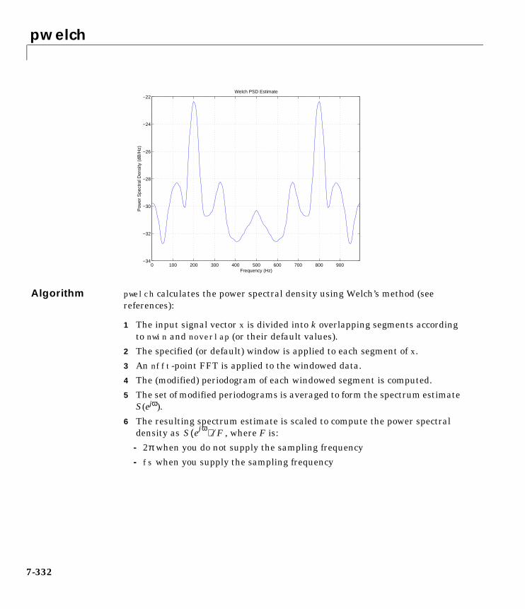
pwelch
7-332
Algorithm pwelch calculates the power spectral density using Welch’s method (seereferences):
1 The input signal vector x is divided into k overlapping segments accordingto nwin and noverlap (or their default values).
2 The specified (or default) window is applied to each segment of x.
3 An nfft-point FFT is applied to the windowed data.
4 The (modified) periodogram of each windowed segment is computed.
5 The set of modified periodograms is averaged to form the spectrum estimateS(ejω).
6 The resulting spectrum estimate is scaled to compute the power spectraldensity as , where F is:
- 2π when you do not supply the sampling frequency
- fs when you supply the sampling frequency
0 100 200 300 400 500 600 700 800 900−34
−32
−30
−28
−26
−24
−22
Frequency (Hz)
Pow
er S
pect
ral D
ensi
ty (
dB/H
z)
Welch PSD Estimate
S ejω( ) F⁄

pwelch
7-333
The number of segments k that x is divided into is calculated as:
• Eight if you don’t specify nwin, or if you specify it as the empty vector []
• if you specify nwin as a nonempty vector or a scalar
In this equation, m is the length of the signal vector x, o is the number ofoverlapping samples (noverlap), and l is the length of each segment (thewindow length).
See Also
References [1] Hayes, M., Statistical Digital Signal Processing and Modeling, John Wiley& Sons, 1996.
k m o–l o–
--------------=
pburg Estimate the power spectral density using the Burgmethod.
pcov Estimate the power spectral density using thecovariance method.
peig Estimate the pseudospectrum using the eigenvectormethod.
periodogram Estimate the power spectral density using aperiodogram.
pmcov Estimate the power spectral density using themodified covariance method.
pmtm Estimate the power spectral density using themultitaper method.
pmusic Estimate the pseudospectrum using the MUSICalgorithm.
psdplot Plot power spectral density data.
pyulear Estimate the power spectral density using theYule-Walker AR method.

pwelch
7-334
[2] Stoica, P., and R.L. Moses, Introduction to Spectral Analysis, Prentice-Hall,Englewood Cliffs, NJ, 1997, pp. 52-54.
[3] Welch, P.D, “The Use of Fast Fourier Transform for the Estimation of PowerSpectra: A Method Based on Time Averaging Over Short, ModifiedPeriodograms,” IEEE Trans. Audio Electroacoustics, Vol. AU-15 (June 1967),pp. 70-73.

pyulear
7-335
7pyulearPurpose Estimate the power spectral density using the Yule-Walker AR method.
Syntax Pxx = pyulear(x,p)[Pxx,w] = pyulear(x,p,nfft)[Pxx,f] = pyulear(x,p,nfft,fs)[Pxx,f] = pyulear(x,p,nfft,fs,'range')[Pxx,w] = pyulear(x,p,nfft,'range')pyulear(...)
Description Pxx = pyulear(x,p) implements the Yule-Walker algorithm, a parametricspectral estimation method, and returns Pxx, an estimate of the power spectraldensity (PSD) of the vector x. The entries of x represent samples of adiscrete-time signal. p is the integer specifying the order of an autoregressive(AR) prediction model for the signal, used in estimating the PSD.
The power spectral density is calculated in units of power per radians persample. Real-valued inputs produce full power one-sided (in frequency) PSDs(by default), while complex-valued inputs produce two-sided PSDs.
In general, the length of the FFT and the values of the input x determine thelength of Pxx and the range of the corresponding normalized frequencies. Forthis syntax, the (default) FFT length is 256. The following table indicates thelength of Pxx and the range of the corresponding normalized frequencies forthis syntax.
[Pxx,w] = pyulear(x,p) also returns w, a vector of frequencies at which thePSD is estimated. Pxx and w have the same length. The units for frequency arerad/sample.
Table 7-37: PSD Vector Characteristics for an FFT Length of 256 (Default)
Real/Complex Input Data
Length of Pxx Range of the Corresponding Normalized Frequencies
Real-valued 129 [0, π]
Complex-valued 256 [0, 2π)

pyulear
7-336
[Pxx,w] = pyulear(x,p,nfft) uses the Yule-walker method to estimate thePSD while specifying the length of the FFT with the integer nfft. If you specifynfft as the empty vector [], it adopts the default value of 256.
The length of Pxx and the frequency range for w depend on nfft and the valuesof the input x. The following table indicates the length of Pxx and the frequencyrange for w for this syntax.
[Pxx,f] = pyulear(x,p,nfft,fs) uses the sampling frequency fs specifiedas an integer in hertz (Hz) to compute the PSD vector (Pxx) and thecorresponding vector of frequencies (f). In this case, the units for the frequencyvector are in Hz. The spectral density produced is calculated in units of powerper Hz. If you specify fs as the empty vector [], the sampling frequencydefaults to 1 Hz.
The frequency range for f depends on nfft, fs, and the values of the input x.The length of Pxx is the same as in Table 7-38. The following table indicates thefrequency range for f for this syntax.
Table 7-38: PSD and Frequency Vector Characteristics
Real/Complex Input Data
nfft Even/Odd Length of Pxx Range of w
Real-valued Even (nfft/2 + 1) [0, π]
Real-valued Odd (nfft + 1)/2 [0, π)
Complex-valued Even or odd nfft [0, 2π)
Table 7-39: PSD and Frequency Vector Characteristics with fs Specified
Real/Complex Input Data nfft Even/Odd Range of f
Real-valued Even [0,fs/2]
Real-valued Odd [0,fs/2)
Complex-valued Even or odd [0,fs)
pyulear
7-337
[Pxx,f] = pyulear(x,p,nfft,fs,'range') or
[Pxx,w] = pyulear(x,p,nfft,'range') specifies the range of frequencyvalues to include in f or w. This syntax is useful when x is real. 'range' can beeither:
• 'twosided': Compute the two-sided PSD over the frequency range [0,fs).This is the default for determining the frequency range forcomplex-valued x.
- If you specify fs as the empty vector, [], the frequency range is [0,1).
- If you don’t specify fs, the frequency range is [0, 2π).
• 'onesided': Compute the one-sided PSD over the frequency ranges specifiedfor real x. This is the default for determining the frequency range forreal-valued x.
Note You can put the string argument 'range' anywhere in the inputargument list after p.
pyulear(...) plots the power spectral density in the current figure window.The frequency range on the plot is the same as the range of output w (or f) fora given set of parameters.
Examples Because the Yule-walker method estimates the spectral density by fitting anAR prediction model of a given order to the signal, first generate a signal froman AR (all-pole) model of a given order. You can use freqz to check themagnitude of the frequency response of your AR filter. This will give you anidea of what to expect when you estimate the PSD using pyulear.
a = [1 -2.2137 2.9403 -2.1697 0.9606]; % AR filter coefficientsfreqz(1,a) % AR filter frequency responsetitle('AR System Frequency Response')
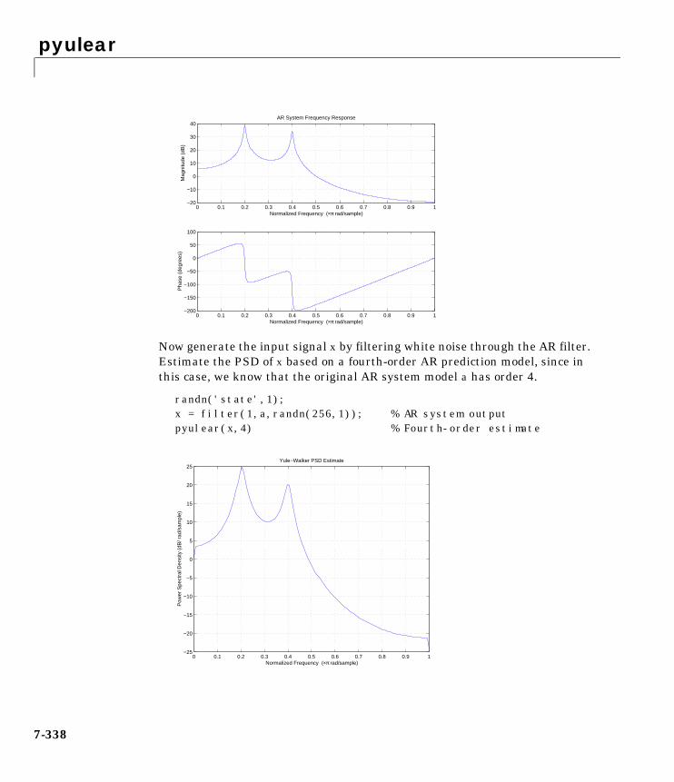
pyulear
7-338
Now generate the input signal x by filtering white noise through the AR filter.Estimate the PSD of x based on a fourth-order AR prediction model, since inthis case, we know that the original AR system model a has order 4.
randn('state',1);x = filter(1,a,randn(256,1)); % AR system outputpyulear(x,4) % Fourth-order estimate
0 0.1 0.2 0.3 0.4 0.5 0.6 0.7 0.8 0.9 1−200
−150
−100
−50
0
50
100
Normalized Frequency (×π rad/sample)
Pha
se (
degr
ees)
0 0.1 0.2 0.3 0.4 0.5 0.6 0.7 0.8 0.9 1−20
−10
0
10
20
30
40
Normalized Frequency (×π rad/sample)
Mag
nitu
de (
dB)
AR System Frequency Response
0 0.1 0.2 0.3 0.4 0.5 0.6 0.7 0.8 0.9 1−25
−20
−15
−10
−5
0
5
10
15
20
25
Normalized Frequency (×π rad/sample)
Pow
er S
pect
ral D
ensi
ty (
dB/ r
ad/s
ampl
e)
Yule−Walker PSD Estimate

pyulear
7-339
Remarks The power spectral density is computed as the distribution of power per unitfrequency.
This algorithm depends on your selecting an appropriate model order for yoursignal.
Algorithm Linear prediction filters can be used to model the second-order statisticalcharacteristics of a signal. The prediction filter output can be used to model thesignal when the input is white noise.
pyulear estimates the PSD of an input signal vector using the Yule-Walker ARmethod. This method, also called the autocorrelation or windowed method, fitsan autoregressive (AR) linear prediction filter model to the signal byminimizing the forward prediction error (based on all observations of the in putsequence) in the least squares sense. This formulation leads to theYule-Walker equations, which are solved by the Levinson-Durbin recursion.The spectral estimate returned by pyulear is the squared magnitude of thefrequency response of this AR model.

pyulear
7-340
See Also
References [1] Marple, S.L., Digital Spectral Analysis, Prentice-Hall, 1987, Chapter 7.
[2] Stoica, P., and R.L. Moses, Introduction to Spectral Analysis, Prentice-Hall,1997.
aryule Compute an estimate of AR model parameters usingthe Yule-Walker method.
lpc Linear prediction coefficients.
pburg Estimate the power spectral density using the Burgmethod.
pcov Estimate the power spectral density using thecovariance method.
peig Estimate the pseudospectrum using the eigenvectormethod.
periodogram Estimate the power spectral density using aperiodogram.
pmcov Estimate the power spectral density using themodified covariance method.
pmtm Estimate the power spectral density using themultitaper method.
pmusic Estimate the pseudospectrum using the MUSICalgorithm.
prony Prony’s method for time domain IIR filter design.
psdplot Plot power spectral density data.
pwelch Estimate the power spectral density using Welch’smethod.
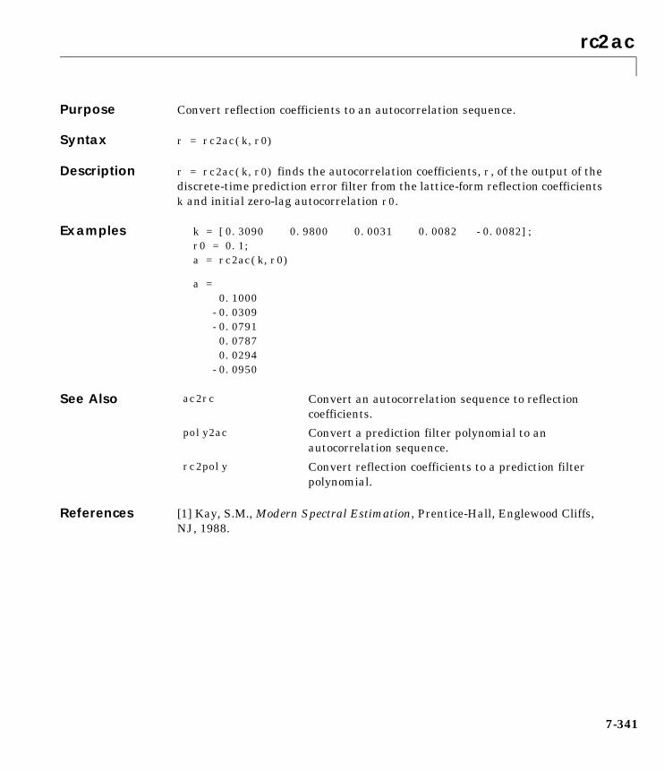
rc2ac
7-341
7rc2acPurpose Convert reflection coefficients to an autocorrelation sequence.
Syntax r = rc2ac(k,r0)
Description r = rc2ac(k,r0) finds the autocorrelation coefficients, r, of the output of thediscrete-time prediction error filter from the lattice-form reflection coefficientsk and initial zero-lag autocorrelation r0.
Examples k = [0.3090 0.9800 0.0031 0.0082 -0.0082];r0 = 0.1;a = rc2ac(k,r0)
a = 0.1000 -0.0309 -0.0791 0.0787 0.0294 -0.0950
See Also
References [1] Kay, S.M., Modern Spectral Estimation, Prentice-Hall, Englewood Cliffs,NJ, 1988.
ac2rc Convert an autocorrelation sequence to reflectioncoefficients.
poly2ac Convert a prediction filter polynomial to anautocorrelation sequence.
rc2poly Convert reflection coefficients to a prediction filterpolynomial.
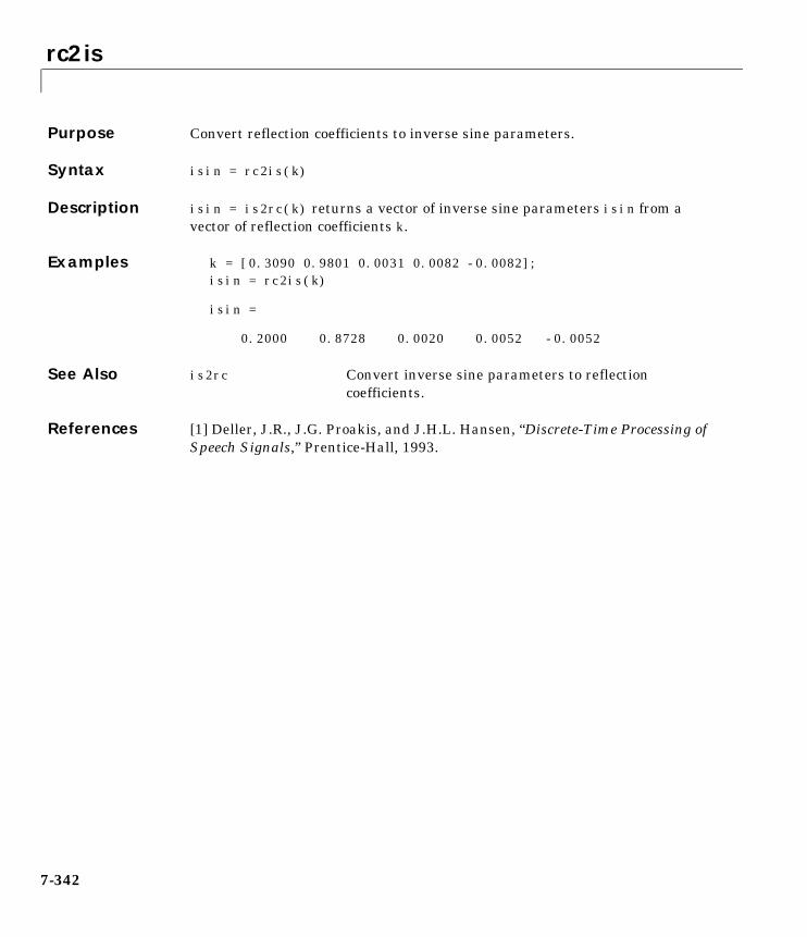
rc2is
7-342
7rc2isPurpose Convert reflection coefficients to inverse sine parameters.
Syntax isin = rc2is(k)
Description isin = is2rc(k) returns a vector of inverse sine parameters isin from avector of reflection coefficients k.
Examples k = [0.3090 0.9801 0.0031 0.0082 -0.0082];isin = rc2is(k)
isin =
0.2000 0.8728 0.0020 0.0052 -0.0052
See Also is2rc Convert inverse sine parameters to reflectioncoefficients.
References [1] Deller, J.R., J.G. Proakis, and J.H.L. Hansen, “Discrete-Time Processing ofSpeech Signals,” Prentice-Hall, 1993.
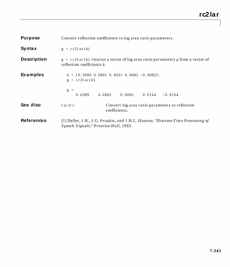
rc2lar
7-343
7rc2larPurpose Convert reflection coefficients to log area ratio parameters.
Syntax g = rc2lar(k)
Description g = rc2lar(k) returns a vector of log area ratio parameters g from a vector ofreflection coefficients k.
Examples k = [0.3090 0.9801 0.0031 0.0082 -0.0082];g = rc2lar(k)
g = 0.6389 4.6002 0.0062 0.0164 -0.0164
See Also lar2rc Convert log area ratio parameters to reflectioncoefficients.
References [1] Deller, J.R., J.G. Proakis, and J.H.L. Hansen, “Discrete-Time Processing ofSpeech Signals,” Prentice-Hall, 1993.
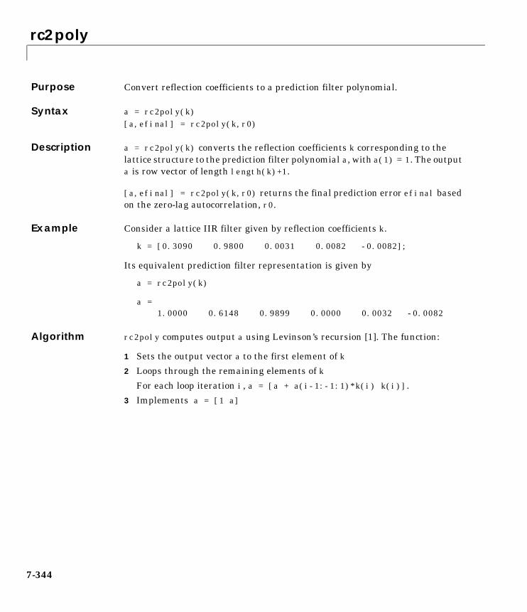
rc2poly
7-344
7rc2polyPurpose Convert reflection coefficients to a prediction filter polynomial.
Syntax a = rc2poly(k)[a,efinal] = rc2poly(k,r0)
Description a = rc2poly(k) converts the reflection coefficients k corresponding to thelattice structure to the prediction filter polynomial a, with a(1) = 1. The outputa is row vector of length length(k)+1.
[a,efinal] = rc2poly(k,r0) returns the final prediction error efinal basedon the zero-lag autocorrelation, r0.
Example Consider a lattice IIR filter given by reflection coefficients k.
k = [0.3090 0.9800 0.0031 0.0082 -0.0082];
Its equivalent prediction filter representation is given by
a = rc2poly(k)
a = 1.0000 0.6148 0.9899 0.0000 0.0032 -0.0082
Algorithm rc2poly computes output a using Levinson’s recursion [1]. The function:
1 Sets the output vector a to the first element of k
2 Loops through the remaining elements of k
For each loop iteration i, a = [a + a(i-1:-1:1)*k(i) k(i)].
3 Implements a = [1 a]
rc2poly
7-345
See Also
References [1] Kay, S.M., Modern Spectral Estimation, Prentice-Hall, Englewood Cliffs,NJ, 1988.
ac2poly Convert an autocorrelation sequence to a predictionfilter polynomial.
latc2tf Lattice filter to transfer function conversion.
latcfilt Lattice and lattice-ladder filter implementation.
poly2rc Convert a prediction filter polynomial to reflectioncoefficients.
rc2ac Convert reflection coefficients to an autocorrelationsequence.
rc2is Convert reflection coefficients to inverse sineparameters.
rc2lar Convert reflection coefficients to log area ratioparameters.
tf2latc Convert transfer function to lattice filter.
rceps
7-346
7rcepsPurpose Real cepstrum and minimum phase reconstruction.
Syntax y = rceps(x)[y,ym] = rceps(x)
Description The real cepstrum is the inverse Fourier transform of the real logarithm of themagnitude of the Fourier transform of a sequence.
rceps(x) returns the real cepstrum of the real sequence x. The real cepstrumis a real-valued function.
[y,ym] = rceps(x) returns both the real cepstrum y and a minimum phasereconstructed version ym of the input sequence.
Algorithm rceps is an M-file implementation of algorithm 7.2 in [2], that is,
y = real(ifft(log(abs(fft(x)))));
Appropriate windowing in the cepstral domain forms the reconstructedminimum phase signal.
w = [1; 2*ones(n/2-1,1); ones(1 - rem(n,2),1); zeros(n/2-1,1)];ym = real(ifft(exp(fft(w.*y))));
See Also
References [1] Oppenheim, A.V., and R.W. Schafer, Digital Signal Processing, EnglewoodCliffs, NJ, Prentice-Hall, 1975.
[2] Programs for Digital Signal Processing, IEEE Press, New York, 1979.
cceps Complex cepstral analysis.
fft One-dimensional fast Fourier transform.
hilbert Hilbert transform.
icceps Inverse complex cepstrum.
unwrap Unwrap phase angles.

rectpuls
7-347
7rectpulsPurpose Generate a sampled aperiodic rectangle.
Syntax y = rectpuls(t)y = rectpuls(t,w)
Description y = rectpuls(t) returns a continuous, aperiodic, unity-height rectangularpulse at the sample times indicated in array t, centered about t = 0 and with adefault width of 1. Note that the interval of non-zero amplitude is defined to beopen on the right, that is, rectpuls(-0.5) = 1 while rectpuls(0.5) = 0.
y = rectpuls(t,w) generates a rectangle of width w.
rectpuls is typically used in conjunction with the pulse train generatingfunction pulstran.
See Also chirp Generate a swept-frequency cosine.
cos Compute the cosine of vector/matrix elements (seethe MATLAB documentation).
diric Compute the Dirichlet or periodic sinc function.
gauspuls Generate a Gaussian-modulated sinusoidal pulse.
pulstran Generate a pulse train.
sawtooth Generate a sawtooth or triangle wave.
sin Compute the sine of vector/matrix elements (see theMATLAB documentation).
sinc Compute the sinc or sin(πt)/πt function.
square Generate a square wave.
tripuls Generate a sampled aperiodic triangle.

remez
7-348
7remezPurpose Compute the Parks-McClellan optimal FIR filter design.
Syntax b = remez(n,f,a)b = remez(n,f,a,w)b = remez(n,f,a,'ftype')b = remez(n,f,a,w,'ftype')b = remez(...,lgrid)b = remez(n,f,'fresp',w)b = remez(n,f,'fresp',w,'ftype')b = remez(n,f,'fresp',p1,p2,...,w)b = remez(n,f,'fresp',p1,p2,...,w,'ftype')[b,delta] = remez(...)[b,delta,opt] = remez(...)
Description remez designs a linear-phase FIR filter using the Parks-McClellanalgorithm [1]. The Parks-McClellan algorithm uses the Remez exchangealgorithm and Chebyshev approximation theory to design filters with anoptimal fit between the desired and actual frequency responses. The filters areoptimal in the sense that the maximum error between the desired frequencyresponse and the actual frequency response is minimized. Filters designed thisway exhibit an equiripple behavior in their frequency responses and aresometimes called equiripple filters.
b = remez(n,f,a) returns row vector b containing the n+1 coefficients of theorder n FIR filter whose frequency-amplitude characteristics match thosegiven by vectors f and a.
The output filter coefficients (taps) in b obey the symmetry relation
b k( ) b n 2 k–+( ) k 1= … n 1+, , ,=

remez
7-349
Vectors f and a specify the frequency-magnitude characteristics of the filter:
• f is a vector of pairs of normalized frequency points, specified in the rangebetween 0 and 1, where 1 corresponds to the Nyquist frequency. Thefrequencies must be in increasing order.
• a is a vector containing the desired amplitudes at the points specified in f.
The desired amplitude at frequencies between pairs of points (f(k), f(k+1)) fork odd is the line segment connecting the points (f(k), a(k)) and(f(k+1), a(k+1)).
The desired amplitude at frequencies between pairs of points (f(k), f(k+1)) fork even is unspecified. The areas between such points are transition or “don’tcare” regions.
• f and a must be the same length. The length must be an even number.
The relationship between the f and a vectors in defining a desired frequencyresponse is shown in the example below.
remez always uses an even filter order for configurations with a passband atthe Nyquist frequency. This is because for odd orders, the frequency responseat the Nyquist frequency is necessarily 0. If you specify an odd-valued n, remezincrements it by 1.
1.0
0.0
Desired amplituderesponse (a)
Normalizedfrequency (f)
0.5
"Don't care"/transition regions
f = [0 .3 .4 .6 .7 .9]a = [0 1 0 0 .5 .5]
0.1 0.2 0.3 0.4 0.5 0.6 0.70.0 0.8 0.9 1.0 (Nyquist)
remez
7-350
remez(n,f,a,w) uses the weights in vector w to weight the fit in each frequencyband. The length of w is half the length of f and a, so there is exactly one weightper band.
b = remez(n,f,a,'ftype') and
b = remez(n,f,a,w,'ftype') specify a filter type, where 'ftype' is
• 'hilbert', for linear-phase filters with odd symmetry (type III and type IV)
The output coefficients in b obey the relation b(k) = -b(n+2-k), k = 1, ...,n + 1. This class of filters includes the Hilbert transformer, which has adesired amplitude of 1 across the entire band.
For example,h = remez(30,[0.1 0.9],[1 1],'hilbert');
designs an approximate FIR Hilbert transformer of length 31.
• 'differentiator', for type III and type IV filters, using a special weightingtechnique
For nonzero amplitude bands, it weights the error by a factor of 1/f so thatthe error at low frequencies is much smaller than at high frequencies. ForFIR differentiators, which have an amplitude characteristic proportional tofrequency, these filters minimize the maximum relative error (the maximumof the ratio of the error to the desired amplitude).
b = remez(...,lgrid) uses the integer lgrid to control the density of thefrequency grid, which has roughly (lgrid*n)/(2*bw) frequency points, wherebw is the fraction of the total frequency band interval [0,1] covered by f.Increasing lgrid often results in filters that more exactly match an equiripplefilter, but that take longer to compute. The default value of 16 is the minimumvalue that should be specified for lgrid. Note that the lgrid argument mustbe a 1-by-1 cell array.
b = remez(n,f,'fresp',w) returns row vector b containing the n+1coefficients of the order n FIR filter whose frequency-amplitude characteristicsbest approximate the response specified by function fresp. The function iscalled from within remez with the following syntax.
[dh,dw] = fresp(n,f,gf,w)
remez
7-351
The arguments are similar to those for remez:
• n is the filter order.
• f is the vector of normalized frequency band edges that appear monotonicallybetween 0 and 1, where 1 is the Nyquist frequency.
• gf is a vector of grid points that have been linearly interpolated over eachspecified frequency band by remez. gf determines the frequency grid atwhich the response function must be evaluated, and contains the same datareturned by cremez in the fgrid field of the opt structure.
• w is a vector of real, positive weights, one per band, used during optimization.w is optional in the call to remez; if not specified, it is set to unity weightingbefore being passed to fresp.
• dh and dw are the desired complex frequency response and band weightvectors, respectively, evaluated at each frequency in grid gf.
The predefined frequency response function fresp that remez calls is remezfrfin the signal/private directory.
b = remez(n,f,'fresp',p1,p2,...,w) allows you to specify additionalparameters (p1, p2, etc.) to pass to fresp. Note that b = remez(n,f,a,w) is asynonym for b = remez(n,f,'remezfrf',a,w), where a is a vectorcontaining the desired amplitudes at the points specified in f.
b = remez(n,f,'fresp',w,'ftype') and
b = remez(n,f,'fresp',p1,p2,...,w,'ftype') design antisymmetric(odd) rather than symmetric (even) filters, where 'ftype' is either 'd' for adifferentiator or 'h' for a Hilbert transformer.
In the absence of a specification for ftype, a preliminary call is made to frespto determine the default symmetry property sym. This call is made using thesyntax.
sym = fresp('defaults',n,f,[],w,p1,p2,...)
The arguments n, f, w, etc., may be used as necessary in determining anappropriate value for sym, which remez expects to be either 'even' or 'odd'. Ifthe fresp function does not support this calling syntax, remez defaults to evensymmetry.
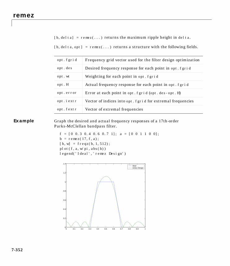
remez
7-352
[b,delta] = remez(...) returns the maximum ripple height in delta.
[b,delta,opt] = remez(...) returns a structure with the following fields.
Example Graph the desired and actual frequency responses of a 17th-orderParks-McClellan bandpass filter.
f = [0 0.3 0.4 0.6 0.7 1]; a = [0 0 1 1 0 0];b = remez(17,f,a);[h,w] = freqz(b,1,512);plot(f,a,w/pi,abs(h))legend('Ideal','remez Design')
opt.fgrid Frequency grid vector used for the filter design optimization
opt.des Desired frequency response for each point in opt.fgrid
opt.wt Weighting for each point in opt.fgrid
opt.H Actual frequency response for each point in opt.fgrid
opt.error Error at each point in opt.fgrid (opt.des-opt.H)
opt.iextr Vector of indices into opt.fgrid for extremal frequencies
opt.fextr Vector of extremal frequencies
0 0.1 0.2 0.3 0.4 0.5 0.6 0.7 0.8 0.9 10
0.2
0.4
0.6
0.8
1
1.2
1.4Ideal remez Design

remez
7-353
Algorithm remez is a MEX-file version of the original Fortran code from [1], altered todesign arbitrarily long filters with arbitrarily many linear bands.
remez designs type I, II, III, and IV linear-phase filters. Type I and type II arethe defaults for n even and n odd, respectively, while type III (n even) andtype IV (n odd) are obtained with the 'hilbert' and 'differentiator' flags.The different types of filters have different symmetries and certain constraintson their frequency responses (see [5] for more details).
Remarks If you get the following warning message,
-– Failure to Converge -–Probable cause is machine rounding error.
it is possible that the filter design may still be correct. Verify the design bychecking its frequency response.
Linear Phase Filter Type
Filter Order
Symmetry of Coefficients Response H(f), f = 0
Response H(f), f = 1 (Nyquist)
Type I Even even: No restriction No restriction
Type II Odd No restriction H(1) = 0
Type III Even odd: H(0) = 0 H(1) = 0
Type IV Odd H(0) = 0 No restriction
b k( ) b n 2 k–+( ) k 1= … n 1+, , ,=
b k( ) b– n 2 k–+( ) k 1= … n 1+, , ,=
remez
7-354
See Also
References [1] Programs for Digital Signal Processing, IEEE Press, New York, 1979,Algorithm 5.1.
[2] Selected Papers in Digital Signal Processing, II, IEEE Press, New York,1979.
[3] Parks, T.W., and C.S. Burrus, Digital Filter Design, John Wiley & Sons,New York:, 1987, p. 83.
[4] Rabiner, L.R., J.H. McClellan, and T.W. Parks, “FIR Digital Filter DesignTechniques Using Weighted Chebyshev Approximations,” Proc. IEEE 63(1975).
butter Design a Butterworth analog and digital filter .
cheby1 Design a Chebyshev type I filter (passband ripple).
cheby2 Design a Chebyshev type II filter (stopband ripple).
cremez Design a complex and nonlinear-phase equirippleFIR filter.
ellip Design an elliptic (Cauer) filter.
fir1 Design a window-based finite impulse response filter:standard response.
fir2 Design a window-based finite impulse response filter:arbitrary response.
fircls Design a constrained least square FIR filter formultiband filters.
fircls1 Design a constrained least square filter for lowpassand highpass linear phase FIR filters.
firls Design a least square linear-phase FIR filter.
firrcos Design a raised cosine FIR filter.
gremez Design a generalized Remez optimal FIR filter design(see the Filter Design Toolbox documentation).
remezord Estimate the Parks-McClellan optimal FIR filterorder.
yulewalk Design a recursive digital filter.

remez
7-355
[5] Oppenheim, A.V., and R.W. Schafer, Discrete-Time Signal Processing,Prentice-Hall, Englewood Cliffs, NJ, 1989, pp. 256-266.
remezord
7-356
7remezordPurpose Parks-McClellan optimal FIR filter order estimation.
Syntax [n,fo,ao,w] = remezord(f,a,dev)[n,fo,ao,w] = remezord(f,a,dev,fs)c = remezord(f,a,dev,fs,'cell')
Description [n,fo,ao,w] = remezord(f,a,dev) finds the approximate order, normalizedfrequency band edges, frequency band amplitudes, and weights that meetinput specifications f, a, and dev.
• f is a vector of frequency band edges (between 0 and fs/2, where fs is thesampling frequency), and a is a vector specifying the desired amplitude onthe bands defined by f. The length of f is two less than twice the length of a.The desired function is piecewise constant.
• dev is a vector the same size as a that specifies the maximum allowabledeviation or ripples between the frequency response and the desiredamplitude of the output filter for each band.
Use remez with the resulting order n, frequency vector fo, amplitude responsevector ao, and weights w to design the filter b which approximately meets thespecifications given by remezord input parameters f, a, and dev.
b = remez(n,fo,ao,w)
[n,fo,ao,w] = remezord(f,a,dev,fs) specifies a sampling frequency fs.fs defaults to 2 Hz, implying a Nyquist frequency of 1 Hz. You can thereforespecify band edges scaled to a particular application’s sampling frequency.
In some cases remezord underestimates the order n. If the filter does not meetthe specifications, try a higher order such as n+1 or n+2.
c = remezord(f,a,dev,fs,'cell') generates a cell-array whose elementsare the parameters to remez.
Examples Example 1Design a minimum-order lowpass filter with a 500 Hz passband cutofffrequency and 600 Hz stopband cutoff frequency, with a sampling frequency of2000 Hz, at least 40 dB attenuation in the stopband, and less than 3 dB ofripple in the passband.
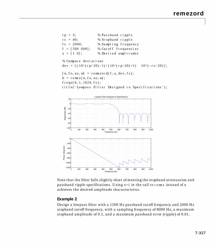
remezord
7-357
rp = 3; % Passband ripplers = 40; % Stopband ripplefs = 2000; % Sampling frequencyf = [500 600]; % Cutoff frequenciesa = [1 0]; % Desired amplitudes
% Compute deviationsdev = [(10^(rp/20)-1)/(10^(rp/20)+1) 10^(-rs/20)];
[n,fo,ao,w] = remezord(f,a,dev,fs);b = remez(n,fo,ao,w);freqz(b,1,1024,fs);title('Lowpass Filter Designed to Specifications');
Note that the filter falls slightly short of meeting the stopband attenuation andpassband ripple specifications. Using n+1 in the call to remez instead of nachieves the desired amplitude characteristics.
Example 2Design a lowpass filter with a 1500 Hz passband cutoff frequency and 2000 Hzstopband cutoff frequency, with a sampling frequency of 8000 Hz, a maximumstopband amplitude of 0.1, and a maximum passband error (ripple) of 0.01.
0 100 200 300 400 500 600 700 800 900 1000−1200
−1000
−800
−600
−400
−200
0
Frequency (Hz)
Ph
ase
(d
eg
ree
s)
0 100 200 300 400 500 600 700 800 900 1000−100
−80
−60
−40
−20
0
20
Frequency (Hz)
Ma
gn
itud
e (
dB
)
Lowpass Filter Designed to Specifications
remezord
7-358
[n,fo,ao,w] = remezord([1500 2000],[1 0],[0.01 0.1],8000 );b = remez(n,fo,ao,w);
This is equivalent to
c = remezord( [1500 2000],[1 0],[0.01 0.1],8000,'cell');b = remez(c:);
Note In some cases, remezord underestimates or overestimates the order n. Ifthe filter does not meet the specifications, try a higher order such as n+1 or n+2.
Results are inaccurate if the cutoff frequencies are near 0 or the Nyquistfrequency.
Algorithm remezord uses the algorithm suggested in [1]. This method is inaccurate forband edges close to either 0 or the Nyquist frequency (fs/2).
See Also
References [1] Rabiner, L.R., and O. Herrmann, “The Predictability of Certain OptimumFinite Impulse Response Digital Filters,” IEEE Trans. on Circuit Theory,Vol. CT-20, No. 4 (July 1973), pp. 401-408.
[2] Rabiner, L.R., and B. Gold. Theory and Application of Digital SignalProcessing. Englewood Cliffs, NJ: Prentice-Hall, 1975, pp. 156-157.
buttord Butterworth filter order selection.
cheb1ord Chebyshev type I filter order selection.
cheb2ord Chebyshev type II filter order selection.
ellipord Elliptic filter order selection.
kaiserord Estimate parameters for an FIR filter design withKaiser window.
remez Parks-McClellan optimal FIR filter design.
resample
7-359
7resamplePurpose Change sampling rate by any rational factor.
Syntax y = resample(x,p,q)y = resample(x,p,q,n)y = resample(x,p,q,n,beta)y = resample(x,p,q,b)[y,b] = resample(x,p,q)
Description y = resample(x,p,q) resamples the sequence in vector x at p/q times theoriginal sampling rate, using a polyphase filter implementation. p and q mustbe positive integers. The length of y is equal to ceil(length(x)*p/q). If x is amatrix, resample works down the columns of x.
resample applies an anti-aliasing (lowpass) FIR filter to x during theresampling process. It designs the filter using firls with a Kaiser window.
y = resample(x,p,q,n) uses n terms on either side of the current sample,x(k), to perform the resampling. The length of the FIR filter resample uses isproportional to n; larger values of n provide better accuracy at the expense ofmore computation time. The default for n is 10. If you let n = 0, resampleperforms a nearest-neighbor interpolation
y(k) = x(round((k-1)*q/p)+1)
where y(k) = 0 if the index to x is greater than length(x).
y = resample(x,p,q,n,beta) uses beta as the design parameter for theKaiser window that resample employs in designing the lowpass filter. Thedefault for beta is 5.
y = resample(x,p,q,b) filters x using the vector of filter coefficients b.
[y,b] = resample(x,p,q) returns the vector b, which contains thecoefficients of the filter applied to x during the resampling process.

resample
7-360
Examples Resample a simple linear sequence at 3/2 the original rate.
fs1 = 10; % Original sampling frequency in Hzt1 = 0:1/fs1:1; % Time vectorx = t1; % Define a linear sequencey = resample(x,3,2); % Now resample it
t2 = (0:(length(y)-1))*2/(3*fs1); % New time vectorplot(t1,x,'*',t2,y,'o',-0.5:0.01:1.5,-0.5:0.01:1.5,':')legend('original','resampled'); xlabel('Time')
Notice that the last few points of the output y are inaccurate. In its filteringprocess, resample assumes the samples at times before and after the givensamples in x are equal to zero. Thus large deviations from zero at the endpoints of the sequence x can cause inaccuracies in y at its end points. Thefollowing two plots illustrate this side effect of resample.
x = [1:10 9:-1:1]; y = resample(x,3,2);subplot(2,1,1);plot(1:19,x,'*',(0:28)*2/3 + 1,y,'o');title('Edge Effects Not Noticeable');legend('original','resampled');
−0.5 0 0.5 1 1.5−0.5
0
0.5
1
1.5
Time
original resampled
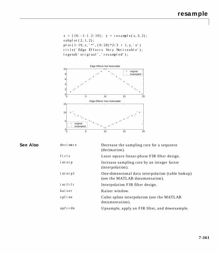
resample
7-361
x = [10:-1:1 2:10]; y = resample(x,3,2);subplot(2,1,2);plot(1:19,x,'*',(0:28)*2/3 + 1,y,'o')title('Edge Effects Very Noticeable');legend('original','resampled');
See Also
0 5 10 15 200
2
4
6
8
10Edge Effects Not Noticeable
original resampled
0 5 10 15 200
5
10
15Edge Effects Very Noticeable
original resampled
decimate Decrease the sampling rate for a sequence(decimation).
firls Least square linear-phase FIR filter design.
interp Increase sampling rate by an integer factor(interpolation).
interp1 One-dimensional data interpolation (table lookup)(see the MATLAB documentation).
intfilt Interpolation FIR filter design.
kaiser Kaiser window.
spline Cubic spline interpolation (see the MATLABdocumentation).
upfirdn Upsample, apply an FIR filter, and downsample.
residuez
7-362
7residuezPurpose z-transform partial-fraction expansion.
Syntax [r,p,k] = residuez(b,a)[b,a] = residuez(r,p,k)
Description residuez converts a discrete time system, expressed as the ratio of twopolynomials, to partial fraction expansion, or residue, form. It also converts thepartial fraction expansion back to the original polynomial coefficients.
[r,p,k] = residuez(b,a) finds the residues, poles, and direct terms of apartial fraction expansion of the ratio of two polynomials, b(z) and a(z).Vectors b and a specify the coefficients of the polynomials of the discrete-timesystem b(z)/a(z) in descending powers of z.
If there are no multiple roots and a > n-1,
The returned column vector r contains the residues, column vector p containsthe pole locations, and row vector k contains the direct terms. The number ofpoles is
n = length(a)-1 = length(r) = length(p)
The direct term coefficient vector k is empty if length(b) is less thanlength(a); otherwise
length(k) = length(b) - length(a) + 1
If p(j) = ... = p(j+s-1) is a pole of multiplicity s, then the expansionincludes terms of the form
b z( ) b0 b1z 1– b2z 2– bmz m–+ + + +=
a z( ) a0 a1z 1– a2z 2– anz n–+ + + +=
b z( )a z( )---------- r 1( )
1 p 1( )z 1––----------------------------
r n( )
1 p n( )z 1––----------------------------- k 1( ) k 2( )z 1– k m n 1+–( )z m n–( )–+ + + + + +=
r j( )
1 p j( )z 1––--------------------------- r j 1+( )
1 p j( )z 1––( )2-----------------------------------
r j sr 1–+( )
1 p j( )z 1––( )sr------------------------------------+ + +
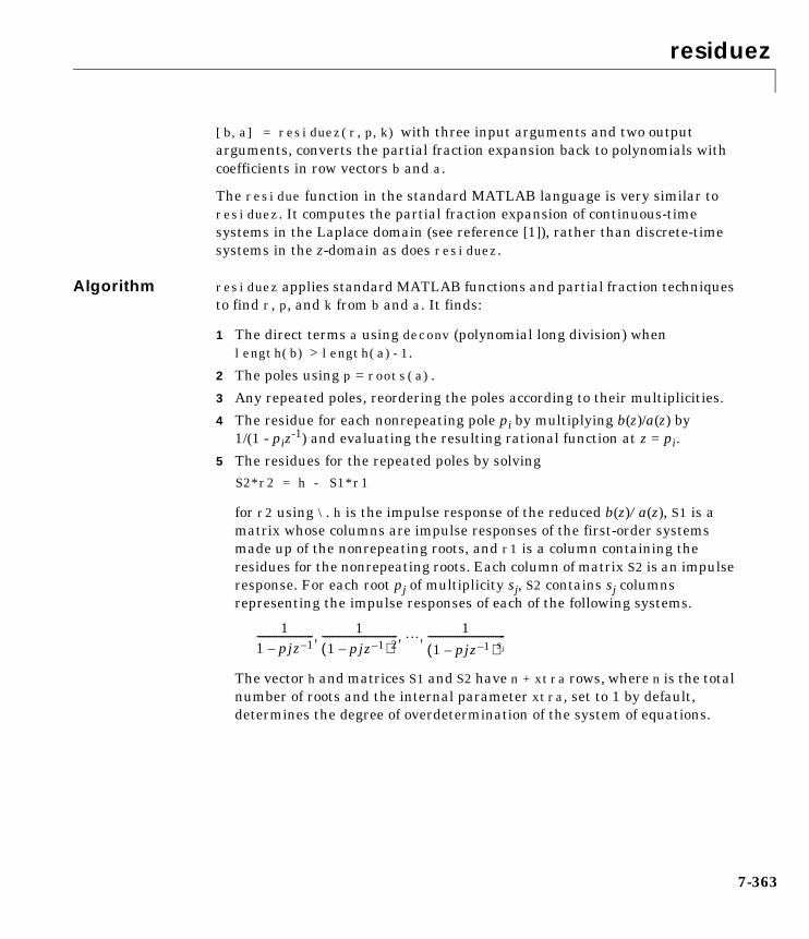
residuez
7-363
[b,a] = residuez(r,p,k) with three input arguments and two outputarguments, converts the partial fraction expansion back to polynomials withcoefficients in row vectors b and a.
The residue function in the standard MATLAB language is very similar toresiduez. It computes the partial fraction expansion of continuous-timesystems in the Laplace domain (see reference [1]), rather than discrete-timesystems in the z-domain as does residuez.
Algorithm residuez applies standard MATLAB functions and partial fraction techniquesto find r, p, and k from b and a. It finds:
1 The direct terms a using deconv (polynomial long division) whenlength(b) > length(a)-1.
2 The poles using p = roots(a).
3 Any repeated poles, reordering the poles according to their multiplicities.
4 The residue for each nonrepeating pole pi by multiplying b(z)/a(z) by1/(1 - piz
-1) and evaluating the resulting rational function at z = pi.
5 The residues for the repeated poles by solvingS2*r2 = h - S1*r1
for r2 using \. h is the impulse response of the reduced b(z)/a(z), S1 is amatrix whose columns are impulse responses of the first-order systemsmade up of the nonrepeating roots, and r1 is a column containing theresidues for the nonrepeating roots. Each column of matrix S2 is an impulseresponse. For each root pj of multiplicity sj, S2 contains sj columnsrepresenting the impulse responses of each of the following systems.
The vector h and matrices S1 and S2 have n + xtra rows, where n is the totalnumber of roots and the internal parameter xtra, set to 1 by default,determines the degree of overdetermination of the system of equations.
11 pjz 1––----------------------- 1
1 pjz 1––( )2-------------------------------
11 pjz 1––( )sj
--------------------------------, , ,
residuez
7-364
See Also
References [1] Oppenheim, A.V., and R.W. Schafer, Digital Signal Processing,Prentice-Hall, Englewood Cliffs, NJ, 1975, pp. 166-170.
convmtx Convolution matrix.
deconv Deconvolution and polynomial division (see theMATLAB documentation).
poly Polynomial with specified roots (see the MATLABdocumentation).
prony Prony’s method for time domain IIR filter design.
residue Partial fraction expansion (see the MATLABdocumentation).
roots Polynomial roots (see the MATLAB documentation).
ss2tf Convert state-space filter parameters tozero-pole-gain form.
tf2ss Convert transfer function filter parameters tostate-space form.
tf2zp Convert transfer function filter parameters tozero-pole-gain form.
zp2ss Convert zero-pole-gain filter parameters tostate-space form.
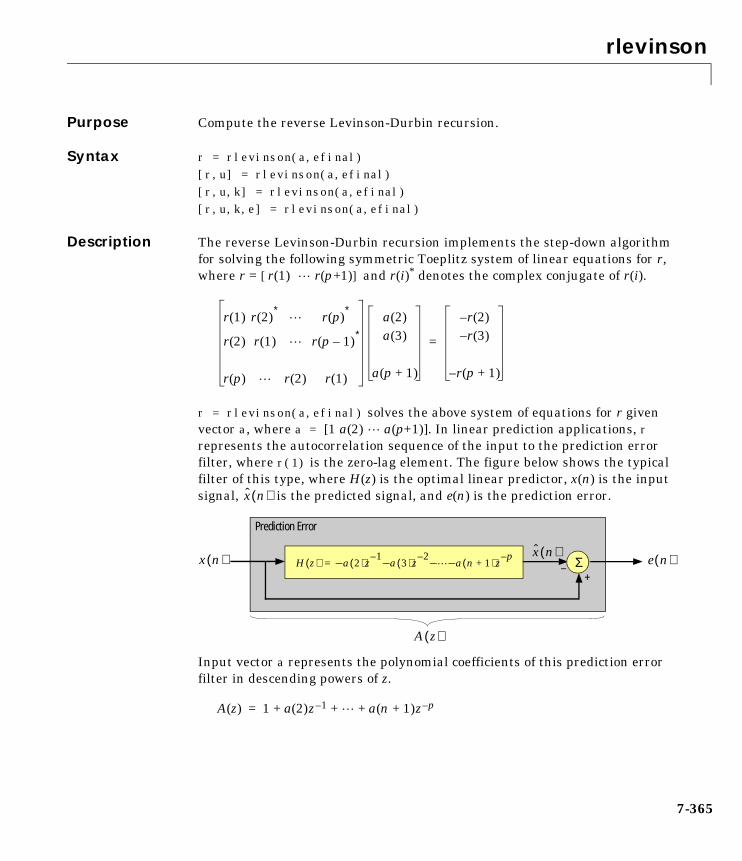
rlevinson
7-365
7rlevinsonPurpose Compute the reverse Levinson-Durbin recursion.
Syntax r = rlevinson(a,efinal)[r,u] = rlevinson(a,efinal)[r,u,k] = rlevinson(a,efinal)[r,u,k,e] = rlevinson(a,efinal)
Description The reverse Levinson-Durbin recursion implements the step-down algorithmfor solving the following symmetric Toeplitz system of linear equations for r,where r = [r(1) r(p+1)] and r(i)* denotes the complex conjugate of r(i).
r = rlevinson(a,efinal) solves the above system of equations for r givenvector a, where a = [1 a(2) a(p+1)]. In linear prediction applications, rrepresents the autocorrelation sequence of the input to the prediction errorfilter, where r(1) is the zero-lag element. The figure below shows the typicalfilter of this type, where H(z) is the optimal linear predictor, x(n) is the inputsignal, is the predicted signal, and e(n) is the prediction error.
Input vector a represents the polynomial coefficients of this prediction errorfilter in descending powers of z.
r 1( ) r 2( )∗
r p( )∗
r 2( ) r 1( ) r p 1–( )∗
r p( ) r 2( ) r 1( )
a 2( )
a 3( )
a p 1+( )
r 2( )–
r 3( )–
r p 1+( )–
=
x n( )
H z( ) a– 2( )z1–
a– 3( )z2–
– a– n 1+( )zp–
= Σx n( )x n( )
–+
e n( )
Prediction Error
A z( )
A z( ) 1 a 2( )z 1– a n 1+( )z p–+ + +=
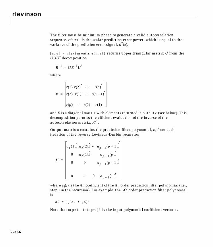
rlevinson
7-366
The filter must be minimum phase to generate a valid autocorrelationsequence. efinal is the scalar prediction error power, which is equal to thevariance of the prediction error signal, σ2(e).
[r,u] = rlevinson(a,efinal) returns upper triangular matrix U from theUDU* decomposition
where
and E is a diagonal matrix with elements returned in output e (see below). Thisdecomposition permits the efficient evaluation of the inverse of theautocorrelation matrix, R-1.
Output matrix u contains the prediction filter polynomial, a, from eachiteration of the reverse Levinson-Durbin recursion
where ai(j) is the jth coefficient of the ith order prediction filter polynomial (i.e.,step i in the recursion). For example, the 5th order prediction filter polynomialis
a5 = u(5:-1:1,5)'
Note that u(p+1:-1:1,p+1)' is the input polynomial coefficient vector a.
R 1– UE 1– U∗=
R
r 1( ) r 2( )∗
r p( )∗
r 2( ) r 1( ) r p 1–( )∗
r p( ) r 2( ) r 1( )
=
U
a1 1( )∗ a2 2( )∗ ap 1+ p 1+( )∗
0 a2 1( )∗ ap 1+ p( )∗
0 0 ap 1+ p 1–( )∗
0 0 ap 1+ 1( )∗
=
rlevinson
7-367
[r,u,k] = rlevinson(a,efinal) returns a vector k of length (p+1) containingthe reflection coefficients. The reflection coefficients are the conjugates of thevalues in the first row of u.
k = conj(u(1,2:end))
[r,u,k,e] = rlevinson(a,efinal) returns a vector of length p+1 containingthe prediction errors from each iteration of the reverse Levinson-Durbinrecursion: e(1) is the prediction error from the first-order model, e(2) is theprediction error from the second-order model, and so on.
These prediction error values form the diagonal of the matrix E in the UDU*
decomposition of R-1.
.
See Also
References [1] Kay, S.M., Modern Spectral Estimation: Theory and Application,Prentice-Hall, Englewood Cliffs, NJ, 1988.
R 1– UE 1– U∗=
levinson Compute the Levinson-Durbin recursion.
lpc Compute linear prediction filter coefficients.
prony Prony’s method for time domain IIR filter design.
stmcb Compute a linear model using Steiglitz-McBrideiteration.

rooteig
7-368
7rooteigPurpose Estimate frequency and power content using the eigenvector method.
Syntax [w,pow] = rooteig(x,p)[f,pow] = rooteig(...,fs)[w,pow] = rooteig(...,'corr')
Description [w,pow] = rooteig(x,p) estimates the frequency content in the time samplesof a signal x, and returns w, a vector of frequencies in rad/sample, and thecorresponding signal power in the vector pow in dB per rad/sample. The inputsignal x is specified either as:
• A row or column vector representing one observation of the signal
• A rectangular array for which each row of x represents a separateobservation of the signal (for example, each row is one output of an array ofsensors, as in array processing), such that x'*x is an estimate of thecorrelation matrix
Note You can use the output of corrmtx to generate such an array x.
You can specify the second input argument p as either:
• A scalar integer. In this case, the signal subspace dimension is p.
• A two-element vector. In this case, p(2), the second element of p, representsa threshold that is multiplied by λmin, the smallest estimated eigenvalue ofthe signal’s correlation matrix. Eigenvalues below the threshold λmin*p(2)are assigned to the noise subspace. In this case, p(1) specifies the maximumdimension of the signal subspace.
The extra threshold parameter in the second entry in p provides you moreflexibility and control in assigning the noise and signal subspaces.
The length of the vector w is the computed dimension of the signal subspace.For real-valued input data x, the length of the corresponding power vector powis given by
length(pow) = 0.5*length(w)
For complex-valued input data x, pow and w have the same length.
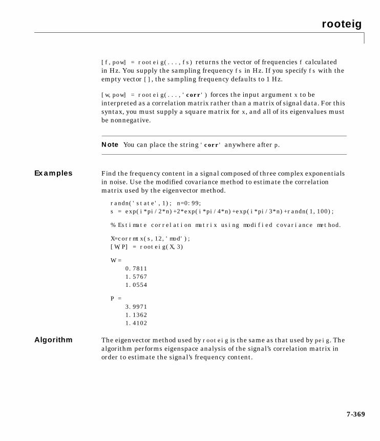
rooteig
7-369
[f,pow] = rooteig(...,fs) returns the vector of frequencies f calculatedin Hz. You supply the sampling frequency fs in Hz. If you specify fs with theempty vector [], the sampling frequency defaults to 1 Hz.
[w,pow] = rooteig(...,'corr') forces the input argument x to beinterpreted as a correlation matrix rather than a matrix of signal data. For thissyntax, you must supply a square matrix for x, and all of its eigenvalues mustbe nonnegative.
Note You can place the string 'corr' anywhere after p.
Examples Find the frequency content in a signal composed of three complex exponentialsin noise. Use the modified covariance method to estimate the correlationmatrix used by the eigenvector method.
randn('state',1); n=0:99; s = exp(i*pi/2*n)+2*exp(i*pi/4*n)+exp(i*pi/3*n)+randn(1,100);
% Estimate correlation matrix using modified covariance method.
X=corrmtx(s,12,'mod'); [W,P] = rooteig(X,3)
W = 0.7811 1.5767 1.0554
P = 3.9971 1.1362 1.4102
Algorithm The eigenvector method used by rooteig is the same as that used by peig. Thealgorithm performs eigenspace analysis of the signal’s correlation matrix inorder to estimate the signal’s frequency content.

rooteig
7-370
The difference between peig and rooteig is:
• peig returns the pseudospectrum at all frequency samples.
• rooteig returns the estimated discrete frequency spectrum, along with thecorresponding signal power estimates.
rooteig is most useful for frequency estimation of signals made up of a sum ofsinusoids embedded in additive white Gaussian noise.
See Also corrmtx Calculate a data matrix for correlation estimation.
peig Estimate the pseudospectrum using the eigenvectormethod.
pmusic Estimate the pseudospectrum using the MUSICalgorithm.
rootmusic Estimate frequency and power content using the rootMUSIC algorithm.

rootmusic
7-371
7rootmusicPurpose Estimate frequency and power content using the root MUSIC algorithm.
Syntax [w,pow] = rootmusic(x,p)[f,pow] = rootmusic(...,fs)[w,pow] = rootmusic(...,'corr')
Description [w,pow] = rootmusic(x,p) estimates the frequency content in the timesamples of a signal x, and returns w, a vector of frequencies in rad/sample, andthe corresponding signal power in the vector pow in dB per rad/sample. Theinput signal x is specified either as:
• A row or column vector representing one observation of the signal
• A rectangular array for which each row of x represents a separateobservation of the signal (for example, each row is one output of an array ofsensors, as in array processing), such that x'*x is an estimate of thecorrelation matrix
Note You can use the output of corrmtx to generate such an array x.
You can specify the second input argument p as either:
• A scalar integer. In this case, the signal subspace dimension is p.
• A two-element vector. In this case, p(2), the second element of p, representsa threshold that is multiplied by λmin, the smallest estimated eigenvalue ofthe signal’s correlation matrix. Eigenvalues below the threshold λmin*p(2)are assigned to the noise subspace. In this case, p(1) specifies the maximumdimension of the signal subspace.
The extra threshold parameter in the second entry in p provides you moreflexibility and control in assigning the noise and signal subspaces.
The length of the vector w is the computed dimension of the signal subspace.For real-valued input data x, the length of the corresponding power vector powis given by
length(pow) = 0.5*length(w)
For complex-valued input data x, pow and w have the same length.
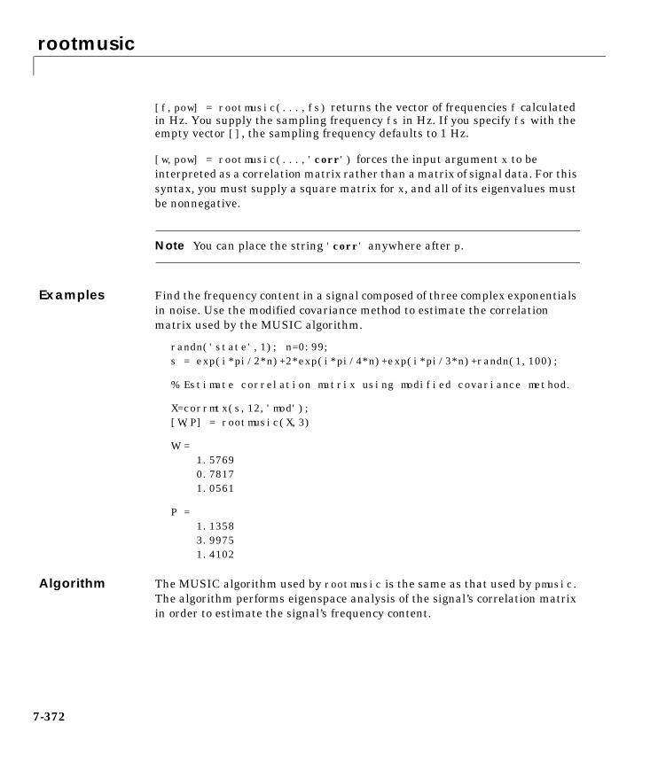
rootmusic
7-372
[f,pow] = rootmusic(...,fs) returns the vector of frequencies f calculatedin Hz. You supply the sampling frequency fs in Hz. If you specify fs with theempty vector [], the sampling frequency defaults to 1 Hz.
[w,pow] = rootmusic(...,'corr') forces the input argument x to beinterpreted as a correlation matrix rather than a matrix of signal data. For thissyntax, you must supply a square matrix for x, and all of its eigenvalues mustbe nonnegative.
Note You can place the string 'corr' anywhere after p.
Examples Find the frequency content in a signal composed of three complex exponentialsin noise. Use the modified covariance method to estimate the correlationmatrix used by the MUSIC algorithm.
randn('state',1); n=0:99; s = exp(i*pi/2*n)+2*exp(i*pi/4*n)+exp(i*pi/3*n)+randn(1,100);
% Estimate correlation matrix using modified covariance method.
X=corrmtx(s,12,'mod'); [W,P] = rootmusic(X,3)
W = 1.5769 0.7817 1.0561
P = 1.1358 3.9975 1.4102
Algorithm The MUSIC algorithm used by rootmusic is the same as that used by pmusic.The algorithm performs eigenspace analysis of the signal’s correlation matrixin order to estimate the signal’s frequency content.

rootmusic
7-373
The difference between pmusic and rootmusic is:
• pmusic returns the pseudospectrum at all frequency samples.
• rootmusic returns the estimated discrete frequency spectrum, along withthe corresponding signal power estimates.
rootmusic is most useful for frequency estimation of signals made up of a sumof sinusoids embedded in additive white Gaussian noise.
See Also corrmtx Calculate a data matrix for correlation estimation.
peig Estimate the pseudospectrum using the eigenvectormethod.
pmusic Estimate the pseudospectrum using the MUSICalgorithm.
rooteig Estimate frequency and power content using the rooteigenvector method.
sawtooth
7-374
7sawtoothPurpose Generate a sawtooth or triangle wave.
Syntax x = sawtooth(t)x = sawtooth(t,width)
Description sawtooth(t) generates a sawtooth wave with period 2π for the elements oftime vector t. sawtooth(t) is similar to sin(t), but creates a sawtooth wavewith peaks of -1 and 1 instead of a sine wave. The sawtooth wave is defined tobe -1 at multiples of 2π and to increase linearly with time with a slope of 1/π atall other times.
sawtooth(t,width) generates a modified triangle wave where width, a scalarparameter between 0 and 1, determines the point between 0 and 2π at whichthe maximum occurs. The function increases from -1 to 1 on the interval 0 to2π*width, then decreases linearly from 1 to -1 on the interval 2π*width to 2π.Thus a parameter of 0.5 specifies a standard triangle wave, symmetric abouttime instant π with peak-to-peak amplitude of 1. sawtooth(t,1) is equivalentto sawtooth(t).
See Also chirp Generate a swept-frequency cosine.
cos Compute the cosine of vector/matrix elements (see theMATLAB documentation).
diric Compute the Dirichlet or periodic sinc function.
gauspuls Generate a Gaussian-modulated sinusoidal pulse.
pulstran Generate a pulse train.
rectpuls Generate a sampled aperiodic rectangle.
sin Compute the sine of vector/matrix elements (see theMATLAB documentation).
sinc Compute the sinc or sin(πt)/πt function.
square Generate a square wave.
tripuls Generate a sampled aperiodic triangle.
schurrc
7-375
7schurrcPurpose Compute reflection coefficients from an autocorrelation sequence.
Syntax k = schurrc(r)[k,e] = schurrc(r)
Description k = schurrc(r) uses the Schur algorithm to compute a vector k of reflectioncoefficients from a vector r representing an autocorrelation sequence. k and rare the same size. The reflection coefficients represent the lattice parametersof a prediction filter for a signal with the given autocorrelation sequence, r.When r is a matrix, schurrc treats each column of r as an independentautocorrelation sequence, and produces a matrix k, the same size as r. Eachcolumn of k represents the reflection coefficients for the lattice filter forpredicting the process with the corresponding autocorrelation sequence r.
[k,e] = schurrc(r) also computes the scalar e, the prediction error variance.When r is a matrix, e is a row vector. The length of e is the same as the numberof columns of r.
Examples Create an autocorrelation sequence from the MATLAB speech signal containedin mtlb.mat, and use the Schur algorithm to compute the reflection coefficientsof a lattice prediction filter for this autocorrelation sequence.
load mtlbr = xcorr(mtlb(1:5),'unbiased');k = schurrc(r(5:end))
k = -0.7583 0.1384 0.7042 -0.3699
See Also levinson Compute a prediction filter using the Levinsonalgorithm.
References [1] Proakis, J. and D. Manolakis, Digital Signal Processing: Principles,Algorithms, and Applications, Third edition, Prentice-Hall, 1996, pp. 868-873.

seqperiod
7-376
7seqperiodPurpose Compute the period of a sequence.
Syntax p = seqperiod(x)[p,num] = seqperiod(x)
Description p = seqperiod(x) returns the integer p that corresponds to the period of thesequence in a vector x. The period p is computed as the minimum length of asubsequence x(1:p) of x that repeats itself continuously every p samples in x.The length of x does not have to be a multiple of p, so that an incompleterepetition is permitted at the end of x. If the sequence x is not periodic, thenp = length(x).
• If x is a matrix, then seqperiod checks for periodicity along each column of x.The resulting output p is a row vector with the same number of columns as x.
• If x is a multidimensional array, then seqperiod checks for periodicity alongthe first nonsingleton dimension of x. In this case:
- p is a multidimensional array of integers with a leading singletondimension.
- The lengths of the remaining dimensions of p correspond to those of thedimensions of x after the first nonsingleton one.
[p,num] = seqperiod(x) also returns the number num of repetitions of x(1:p)in x. num might not be an integer.
Examples x = [4 0 1 6; 2 0 2 7; 4 0 1 5; 2 0 5 6];
p = seqperiod(x)
p = 2 1 4 3

seqperiod
7-377
The result implies:
• The first column of x has period 2.
• The second column of x has period 1.
• The third column of x is not periodic, so p(3) is just the number of rows of x.
• The fourth column of x has period 3, although the last (second) repetition ofthe periodic sequence is incomplete.
sgolay
7-378
7sgolayPurpose Savitzky-Golay filter design.
Syntax b = sgolay(k,f)b = sgolay(k,f,w)
Description b = sgolay(k,f) designs a Savitzky-Golay FIR smoothing filter b. Thepolynomial order k must be less than the frame size, f, which must be odd. Ifk = f-1, the designed filter produces no smoothing. The output, b, is an f-by-fmatrix whose rows represent the time-varying FIR filter coefficients. In asmoothing filter implementation (for example, sgolayfilt), the last (f-1)/2rows (each an FIR filter) are applied to the signal during the startup transient,and the first (f-1)/2 rows are applied to the signal during the terminaltransient. The center row is applied to the signal in the steady state.
b = sgolay(k,f,w) specifies a weighting vector w with length f, whichcontains the real, positive-valued weights to be used during the least-squaresminimization.
Remarks Savitzky-Golay smoothing filters (also called digital smoothing polynomialfilters or least squares smoothing filters) are typically used to “smooth out” anoisy signal whose frequency span (without noise) is large. In this type ofapplication, Savitzky-Golay smoothing filters perform much better thanstandard averaging FIR filters, which tend to filter out a significant portion ofthe signal’s high frequency content along with the noise. AlthoughSavitzky-Golay filters are more effective at preserving the pertinent highfrequency components of the signal, they are less successful than standardaveraging FIR filters at rejecting noise.
Savitzky-Golay filters are optimal in the sense that they minimize theleast-squares error in fitting a polynomial to each frame of noisy data.
See Also fir1 Window-based finite impulse response filter design –standard response.
firls Least square linear-phase FIR filter design.
filter Filter data with a recursive (IIR) or nonrecursive(FIR) filter.
sgolayfilt Savitzky-Golay filtering.

sgolay
7-379
References [1] Orfanidis, S.J., Introduction to Signal Processing, Prentice-Hall, EnglewoodCliffs, NJ, 1996.
sgolayfilt
7-380
7sgolayfiltPurpose Savitzky-Golay filtering.
Syntax y = sgolayfilt(x,k,f)y = sgolayfilt(x,k,f,w)
Description y = sgolayfilt(x,k,f) applies a Savitzky-Golay FIR smoothing filter to thedata in vector x. If x is a matrix, sgolayfilt operates on each column. Thepolynomial order k must be less than the frame size, f, which must be odd. Ifk = f-1, the filter produces no smoothing.
y = sgolayfilt(x,k,f,w) specifies a weighting vector w with length f, whichcontains the real, positive-valued weights to be used during the least-squaresminimization.
Remarks Savitzky-Golay smoothing filters (also called digital smoothing polynomialfilters or least-squares smoothing filters) are typically used to “smooth out” anoisy signal whose frequency span (without noise) is large. In this type ofapplication, Savitzky-Golay smoothing filters perform much better thanstandard averaging FIR filters, which tend to filter out a significant portion ofthe signal’s high frequency content along with the noise. AlthoughSavitzky-Golay filters are more effective at preserving the pertinent highfrequency components of the signal, they are less successful than standardaveraging FIR filters at rejecting noise.
Savitzky-Golay filters are optimal in the sense that they minimize theleast-squares error in fitting a polynomial to frames of noisy data.
Example Smooth the mtlb signal by applying a cubic Savitzky-Golay filter to dataframes of length 41.
load mtlb % Load the data.smtlb = sgolayfilt(mtlb,3,41); % Apply the 3rd-order filter.
subplot(2,1,1)plot([1:2000],mtlb(1:2000)); axis([0 2000 -4 4]);title('mtlb'); grid;
subplot(2,1,2)plot([1:2000],smtlb(1:2000)); axis([0 2000 -4 4]);title('smtlb'); grid;
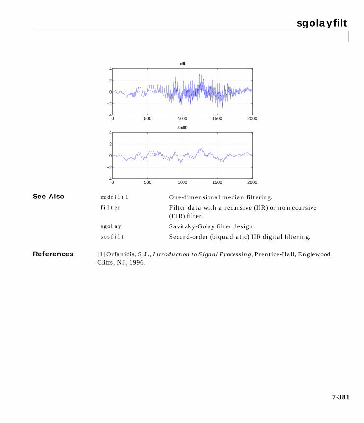
sgolayfilt
7-381
See Also
References [1] Orfanidis, S.J., Introduction to Signal Processing, Prentice-Hall, EnglewoodCliffs, NJ, 1996.
0 500 1000 1500 2000−4
−2
0
2
4mtlb
0 500 1000 1500 2000−4
−2
0
2
4smtlb
medfilt1 One-dimensional median filtering.
filter Filter data with a recursive (IIR) or nonrecursive(FIR) filter.
sgolay Savitzky-Golay filter design.
sosfilt Second-order (biquadratic) IIR digital filtering.
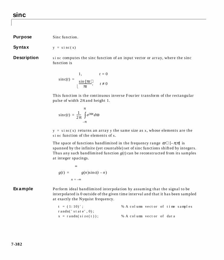
sinc
7-382
7sincPurpose Sinc function.
Syntax y = sinc(x)
Description sinc computes the sinc function of an input vector or array, where the sincfunction is
This function is the continuous inverse Fourier transform of the rectangularpulse of width 2π and height 1.
y = sinc(x) returns an array y the same size as x, whose elements are thesinc function of the elements of x.
The space of functions bandlimited in the frequency range isspanned by the infinite (yet countable) set of sinc functions shifted by integers.Thus any such bandlimited function g(t) can be reconstructed from its samplesat integer spacings.
Example Perform ideal bandlimited interpolation by assuming that the signal to beinterpolated is 0 outside of the given time interval and that it has been sampledat exactly the Nyquist frequency.
t = (1:10)'; % A column vector of time samplesrandn('state',0);x = randn(size(t)); % A column vector of data
sinc t( )1 t 0=,
πt( )sinπt
------------------- t 0≠,
=
sinc t( )1
2π------ ejωt ωd
π–
π
=
ω π– π[ , ]∈
g t( ) g n( )sinc t n–( )
n ∞–=
∞
=
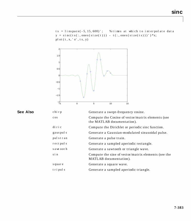
sinc
7-383
ts = linspace(-5,15,600)'; % times at which to interpolate datay = sinc(ts(:,ones(size(t))) - t(:,ones(size(ts)))')*x;plot(t,x,'o',ts,y)
See Also
−5 0 5 10 15−2
−1.5
−1
−0.5
0
0.5
1
1.5
2
chirp Generate a swept-frequency cosine.
cos Compute the Cosine of vector/matrix elements (seethe MATLAB documentation).
diric Compute the Dirichlet or periodic sinc function.
gauspuls Generate a Gaussian-modulated sinusoidal pulse.
pulstran Generate a pulse train.
rectpuls Generate a sampled aperiodic rectangle.
sawtooth Generate a sawtooth or triangle wave.
sin Compute the sine of vector/matrix elements (see theMATLAB documentation).
square Generate a square wave.
tripuls Generate a sampled aperiodic triangle.
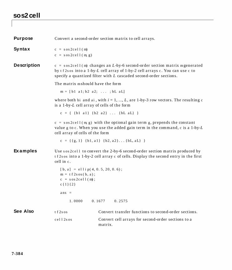
sos2cell
7-384
7sos2cellPurpose Convert a second-order section matrix to cell arrays.
Syntax c = sos2cell(m)
c = sos2cell(m,g)
Description c = sos2cell(m) changes an L-by-6 second-order section matrix m generatedby tf2sos into a 1-by-L cell array of 1-by-2 cell arrays c. You can use c tospecify a quantized filter with L cascaded second-order sections.
The matrix m should have the form
m = [b1 a1;b2 a2; ... ;bL aL]
where both bi and ai, with i = 1, ..., L, are 1-by-3 row vectors. The resulting cis a 1-by-L cell array of cells of the form
c = b1 a1 b2 a2 ... bL aL
c = sos2cell(m,g) with the optional gain term g, prepends the constantvalue g to c. When you use the added gain term in the command, c is a 1-by-Lcell array of cells of the form
c = g,1 b1,a1 b2,a2...bL,aL
Examples Use sos2cell to convert the 2-by-6 second-order section matrix produced bytf2sos into a 1-by-2 cell array c of cells. Display the second entry in the firstcell in c.
[b,a] = ellip(4,0.5,20,0.6);m = tf2sos(b,a);c = sos2cell(m);c12
ans =
1.0000 0.1677 0.2575
See Also tf2sos Convert transfer functions to second-order sections.
cell2sos Convert cell arrays for second-order sections to amatrix.

sos2ss
7-385
7sos2ssPurpose Convert digital filter second-order section parameters to state-space form.
Syntax [A,B,C,D] = sos2ss(sos)[A,B,C,D] = sos2ss(sos,g)
Description sos2ss converts a second-order section representation of a given digital filterto an equivalent state-space representation.
[A,B,C,D] = sos2ss(sos) converts the system sos, in second-order sectionform, to a single-input, single-output state-space representation.
The discrete transfer function in second-order section form is given by
sos is a L-by-6 matrix organized as
The entries of sos must be real for proper conversion to state space. Thereturned matrix A is size N-by-N, where N = 2L-1, B is a length N-1 columnvector, C is a length N-1 row vector, and D is a scalar.
[A,B,C,D] = sos2ss(sos,g) converts the system sos in second-order sectionform with gain g.
x n 1+[ ] Ax n[ ] Bu n[ ]+=
y n[ ] Cx n[ ] Du n[ ]+=
H z( ) Hk z( )
k 1=
L
∏b0k b1kz 1– b2kz 2–+ +
1 a1kz 1– a2kz 2–+ +----------------------------------------------------------
k 1=
L
∏= =
sos
b01 b11 b21 1 a11 a21
b02 b12 b22 1 a12 a22
b0L b1L b2L 1 a1L a2L
=
H z( ) g Hk z( )
k 1=
L
∏=
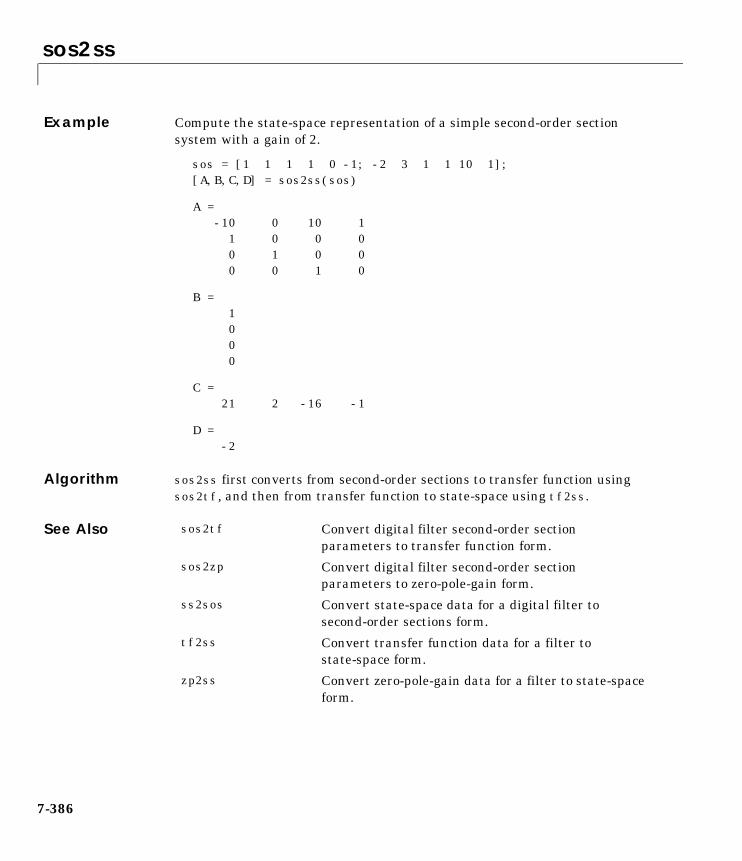
sos2ss
7-386
Example Compute the state-space representation of a simple second-order sectionsystem with a gain of 2.
sos = [1 1 1 1 0 -1; -2 3 1 1 10 1];[A,B,C,D] = sos2ss(sos)
A = -10 0 10 1 1 0 0 0 0 1 0 0 0 0 1 0
B = 1 0 0 0
C = 21 2 -16 -1
D = -2
Algorithm sos2ss first converts from second-order sections to transfer function usingsos2tf, and then from transfer function to state-space using tf2ss.
See Also sos2tf Convert digital filter second-order sectionparameters to transfer function form.
sos2zp Convert digital filter second-order sectionparameters to zero-pole-gain form.
ss2sos Convert state-space data for a digital filter tosecond-order sections form.
tf2ss Convert transfer function data for a filter tostate-space form.
zp2ss Convert zero-pole-gain data for a filter to state-spaceform.
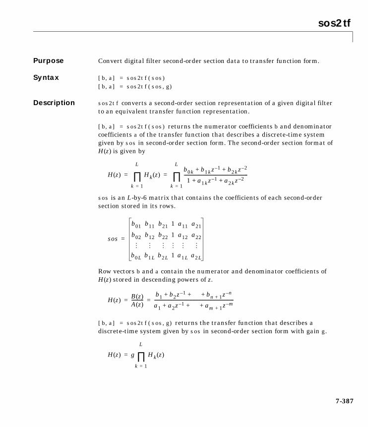
sos2tf
7-387
7sos2tfPurpose Convert digital filter second-order section data to transfer function form.
Syntax [b,a] = sos2tf(sos)[b,a] = sos2tf(sos,g)
Description sos2tf converts a second-order section representation of a given digital filterto an equivalent transfer function representation.
[b,a] = sos2tf(sos) returns the numerator coefficients b and denominatorcoefficients a of the transfer function that describes a discrete-time systemgiven by sos in second-order section form. The second-order section format ofH(z) is given by
sos is an L-by-6 matrix that contains the coefficients of each second-ordersection stored in its rows.
Row vectors b and a contain the numerator and denominator coefficients ofH(z) stored in descending powers of z.
[b,a] = sos2tf(sos,g) returns the transfer function that describes adiscrete-time system given by sos in second-order section form with gain g.
H z( ) Hk z( )
k 1=
L
∏b0k b1kz 1– b2kz 2–+ +
1 a1kz 1– a2kz 2–+ +----------------------------------------------------------
k 1=
L
∏= =
sos
b01 b11 b21 1 a11 a21
b02 b12 b22 1 a12 a22
b0L b1L b2L 1 a1L a2L
=
H z( )B z( )A z( )-----------
b1 b2z 1– bn 1+ z n–+ + +
a1 a2z 1– am 1+ z m–+ + +------------------------------------------------------------------------= =
H z( ) g Hk z( )
k 1=
L
∏=
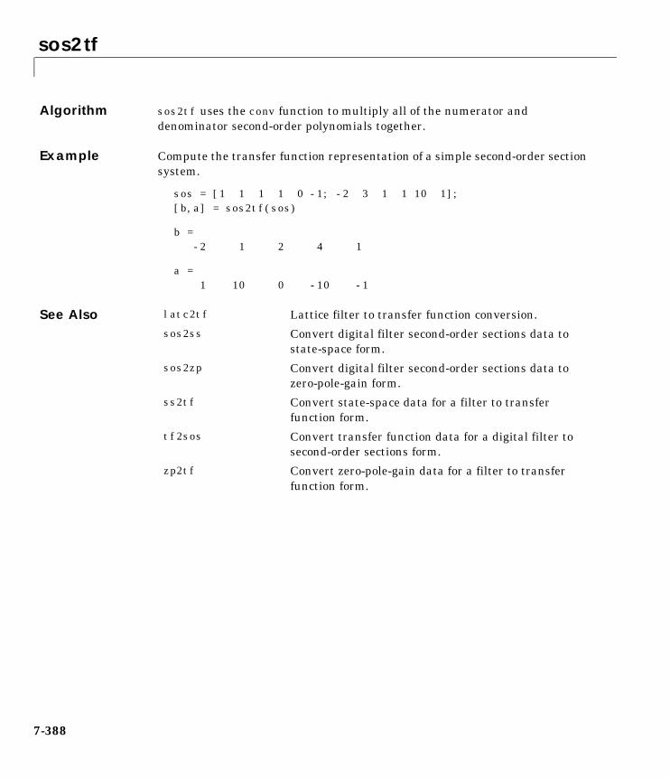
sos2tf
7-388
Algorithm sos2tf uses the conv function to multiply all of the numerator anddenominator second-order polynomials together.
Example Compute the transfer function representation of a simple second-order sectionsystem.
sos = [1 1 1 1 0 -1; -2 3 1 1 10 1];[b,a] = sos2tf(sos)
b = -2 1 2 4 1
a = 1 10 0 -10 -1
See Also latc2tf Lattice filter to transfer function conversion.
sos2ss Convert digital filter second-order sections data tostate-space form.
sos2zp Convert digital filter second-order sections data tozero-pole-gain form.
ss2tf Convert state-space data for a filter to transferfunction form.
tf2sos Convert transfer function data for a digital filter tosecond-order sections form.
zp2tf Convert zero-pole-gain data for a filter to transferfunction form.
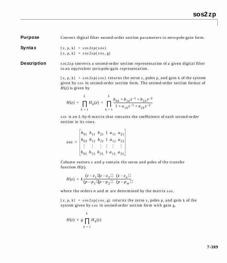
sos2zp
7-389
7sos2zpPurpose Convert digital filter second-order section parameters to zero-pole-gain form.
Syntax [z,p,k] = sos2zp(sos)[z,p,k] = sos2zp(sos,g)
Description sos2zp converts a second-order section representation of a given digital filterto an equivalent zero-pole-gain representation.
[z,p,k] = sos2zp(sos) returns the zeros z, poles p, and gain k of the systemgiven by sos in second-order section form. The second-order section format ofH(z) is given by
sos is an L-by-6 matrix that contains the coefficients of each second-ordersection in its rows.
Column vectors z and p contain the zeros and poles of the transferfunction H(z).
where the orders n and m are determined by the matrix sos.
[z,p,k] = sos2zp(sos,g) returns the zeros z, poles p, and gain k of thesystem given by sos in second-order section form with gain g.
H z( ) Hk z( )
k 1=
L
∏b0k b1kz 1– b2kz 2–+ +
1 a1kz 1– a2kz 2–+ +----------------------------------------------------------
k 1=
L
∏= =
sos
b01 b11 b21 1 a11 a21
b02 b12 b22 1 a12 a22
b0L b1L b2L 1 a1L a2L
=
H z( ) kz z1–( ) z z2–( ) z zn–( )
p p1–( ) p p2–( ) p pm–( )----------------------------------------------------------------------=
H z( ) g Hk z( )
k 1=
L
∏=
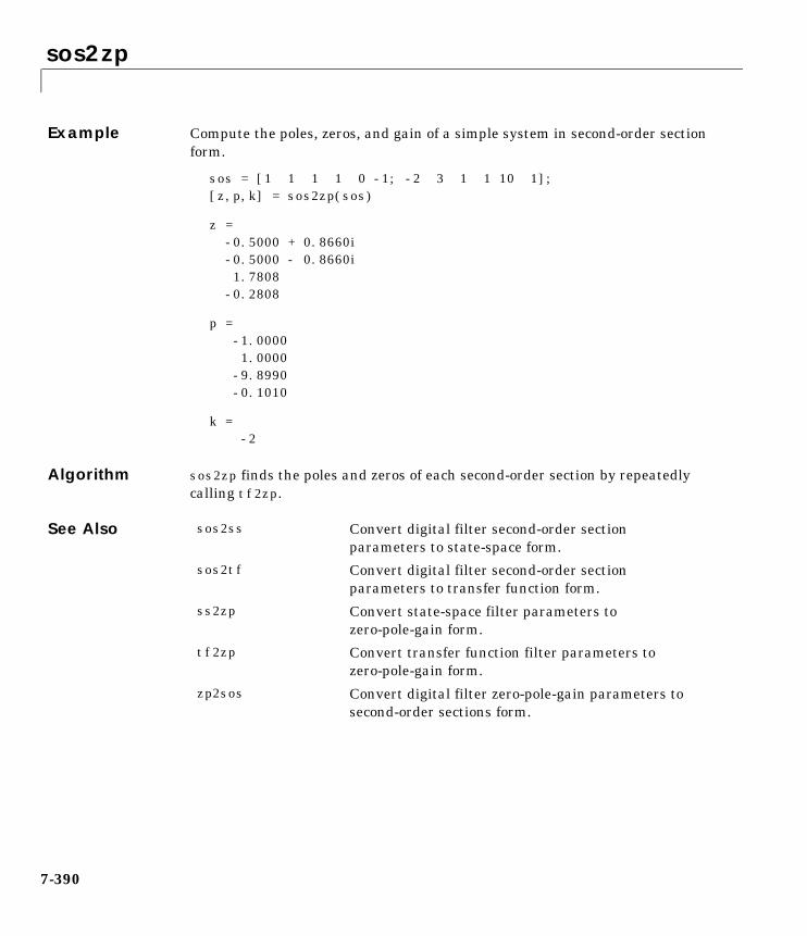
sos2zp
7-390
Example Compute the poles, zeros, and gain of a simple system in second-order sectionform.
sos = [1 1 1 1 0 -1; -2 3 1 1 10 1];[z,p,k] = sos2zp(sos)
z = -0.5000 + 0.8660i -0.5000 - 0.8660i 1.7808 -0.2808
p = -1.0000 1.0000 -9.8990 -0.1010
k = -2
Algorithm sos2zp finds the poles and zeros of each second-order section by repeatedlycalling tf2zp.
See Also sos2ss Convert digital filter second-order sectionparameters to state-space form.
sos2tf Convert digital filter second-order sectionparameters to transfer function form.
ss2zp Convert state-space filter parameters tozero-pole-gain form.
tf2zp Convert transfer function filter parameters tozero-pole-gain form.
zp2sos Convert digital filter zero-pole-gain parameters tosecond-order sections form.
sosfilt
7-391
7sosfiltPurpose Second-order (biquadratic) IIR digital filtering.
Syntax y = sosfilt(sos,x)
Description y = sosfilt(sos,x) applies the second-order section digital filter sos to thevector x. The output, y, is the same length as x.
sos represents the second-order section digital filter H(z)
by an L-by-6 matrix containing the coefficients of each second-order section inits rows.
If x is a matrix, sosfilt applies the filter to each column of x independently.Output y is a matrix of the same size, containing the filtered datacorresponding to each column of x.
See Also
References [1] Orfanidis, S.J., Introduction to Signal Processing, Prentice-Hall, EnglewoodCliffs, NJ, 1996.
H z( ) Hk z( )
k 1=
L
∏b0k b1kz 1– b2kz 2–+ +
1 a1kz 1– a2kz 2–+ +----------------------------------------------------------
k 1=
L
∏= =
sos
b01 b11 b21 1 a11 a21
b02 b12 b22 1 a12 a22
b0L b1L b2L 1 a1L a2L
=
filter Apply a filter to data.
medfilt1 One-dimensional median filtering.
sgolayfilt Savitzky-Golay filtering.
specgram
7-392
7specgramPurpose Time-dependent frequency analysis (spectrogram).
Syntax B = specgram(a)B = specgram(a,nfft)[B,f] = specgram(a,nfft,fs)[B,f,t] = specgram(a,nfft,fs)B = specgram(a,nfft,fs,window)B = specgram(a,nfft,fs,window,numoverlap)specgram(a)B = specgram(a,f,fs,window,numoverlap)
Description specgram computes the windowed discrete-time Fourier transform of a signalusing a sliding window. The spectrogram is the magnitude of this function.
B = specgram(a) calculates the spectrogram for the signal in vector a. Thissyntax uses the default values:
• nfft = min(256,length(a))
• fs = 2
• window is a periodic Hann (Hanning) window of length nfft.• numoverlap = length(window)/2
nfft specifies the FFT length that specgram uses. This value determines thefrequencies at which the discrete-time Fourier transform is computed. fs is ascalar that specifies the sampling frequency. window specifies a windowingfunction and the number of samples specgram uses in its sectioning of vector a.numoverlap is the number of samples by which the sections overlap. Anyarguments that you omit from the end of the input parameter list use thedefault values shown above.
If a is real, specgram computes the discrete-time Fourier transform at positivefrequencies only. If n is even, specgram returns nfft/2+1 rows (including thezero and Nyquist frequency terms). If n is odd, specgram returns nfft/2 rows.The number of columns in B is
k = fix((n-numoverlap)/(length(window)-numoverlap))
If a is complex, specgram computes the discrete-time Fourier transform at bothpositive and negative frequencies. In this case, B is a complex matrix with nfft

specgram
7-393
rows. Time increases linearly across the columns of B, starting with sample 1in column 1. Frequency increases linearly down the rows, starting at 0.
B = specgram(a,nfft) uses the specified FFT length nfft in its calculations.
[B,f] = specgram(a,nfft,fs) returns a vector f of frequencies at which thefunction computes the discrete-time Fourier transform. fs has no effect on theoutput B; it is a frequency scaling multiplier.
[B,f,t] = specgram(a,nfft,fs) returns frequency and time vectors f and trespectively. t is a column vector of scaled times, with length equal to thenumber of columns of B. t(j) is the earliest time at which the jth windowintersects a. t(1) is always equal to 0.
B = specgram(a,nfft,fs,window) specifies a windowing function and thenumber of samples per section of the x vector. If you supply a scalar for window,specgram uses a Hann window of that length. The length of the window mustbe less than or equal to nfft.
B = specgram(a,nfft,fs,window,numoverlap) overlaps the sections of x bynumoverlap samples.
You can use the empty matrix [] to specify the default value for any inputargument. For example,
B = specgram(x,[],10000)
is equivalent to
B = specgram(x)
but with a sampling frequency of 10,000 Hz instead of the default 2 Hz.
specgram(...) with no output arguments displays the scaled logarithm of thespectrogram in the current figure window using
imagesc(t,f,20*log10(abs(b))), axis xy, colormap(jet)
The axis xy mode displays the low-frequency content of the first portion of thesignal in the lower-left corner of the axes. specgram uses fs to label the axesaccording to true time and frequency.
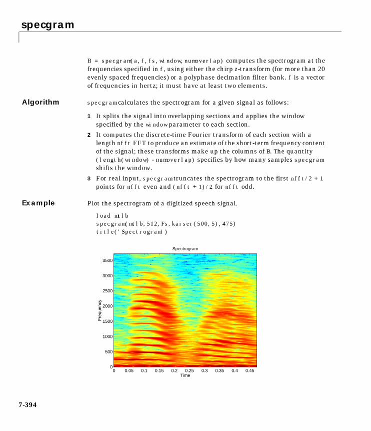
specgram
7-394
B = specgram(a,f,fs,window,numoverlap) computes the spectrogram at thefrequencies specified in f, using either the chirp z-transform (for more than 20evenly spaced frequencies) or a polyphase decimation filter bank. f is a vectorof frequencies in hertz; it must have at least two elements.
Algorithm specgram calculates the spectrogram for a given signal as follows:
1 It splits the signal into overlapping sections and applies the windowspecified by the window parameter to each section.
2 It computes the discrete-time Fourier transform of each section with alength nfft FFT to produce an estimate of the short-term frequency contentof the signal; these transforms make up the columns of B. The quantity(length(window) - numoverlap) specifies by how many samples specgramshifts the window.
3 For real input, specgram truncates the spectrogram to the first nfft/2 + 1points for nfft even and (nfft + 1)/2 for nfft odd.
Example Plot the spectrogram of a digitized speech signal.
load mtlbspecgram(mtlb,512,Fs,kaiser(500,5),475)title('Spectrogram')
Time
Fre
quen
cy
Spectrogram
0 0.05 0.1 0.15 0.2 0.25 0.3 0.35 0.4 0.450
500
1000
1500
2000
2500
3000
3500

specgram
7-395
Diagnostics An appropriate diagnostic message is displayed when incorrect arguments areused.
Requires window's length to be no greater than the FFT length.Requires NOVERLAP to be strictly less than the window length.Requires positive integer values for NFFT and NOVERLAP.Requires vector input.
See Also
References [1] Oppenheim, A.V., and R.W. Schafer, Discrete-Time Signal Processing,Prentice-Hall, Englewood Cliffs, NJ, 1989, pp. 713-718.
[2] Rabiner, L.R., and R.W. Schafer, Digital Processing of Speech Signals,Prentice-Hall, Englewood Cliffs, NJ, 1978.
cohere Estimate magnitude squared coherence functionbetween two signals.
csd Estimate the cross spectral density (CSD) of twosignals.
pwelch Estimate the power spectral density (PSD) of a signalusing Welch’s method.
tfe Transfer function estimate from input and output.
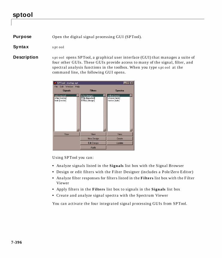
sptool
7-396
7sptoolPurpose Open the digital signal processing GUI (SPTool).
Syntax sptool
Description sptool opens SPTool, a graphical user interface (GUI) that manages a suite offour other GUIs. These GUIs provide access to many of the signal, filter, andspectral analysis functions in the toolbox. When you type sptool at thecommand line, the following GUI opens.
Using SPTool you can:
• Analyze signals listed in the Signals list box with the Signal Browser
• Design or edit filters with the Filter Designer (includes a Pole/Zero Editor)
• Analyze filter responses for filters listed in the Filters list box with the FilterViewer
• Apply filters in the Filters list box to signals in the Signals list box
• Create and analyze signal spectra with the Spectrum Viewer
You can activate the four integrated signal processing GUIs from SPTool.
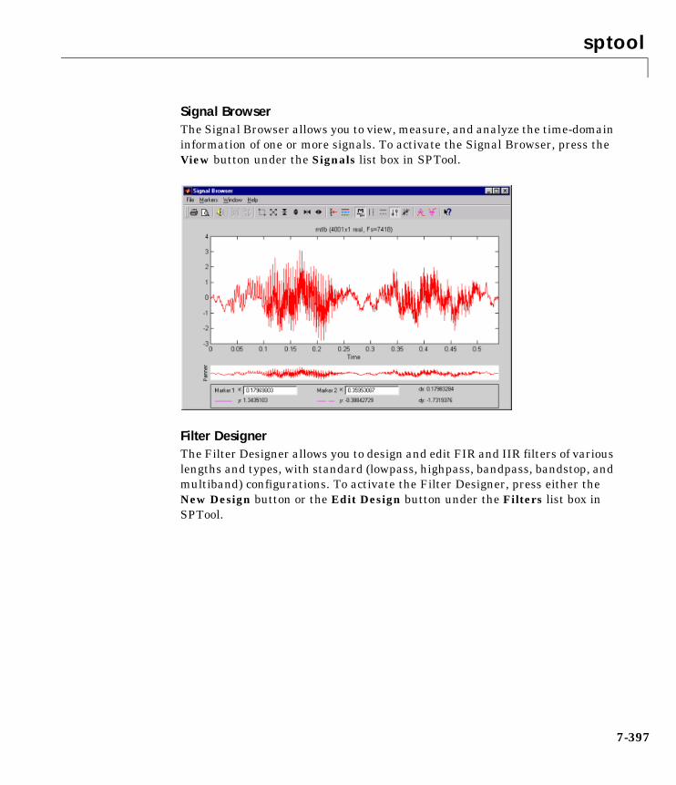
sptool
7-397
Signal BrowserThe Signal Browser allows you to view, measure, and analyze the time-domaininformation of one or more signals. To activate the Signal Browser, press theView button under the Signals list box in SPTool.
Filter DesignerThe Filter Designer allows you to design and edit FIR and IIR filters of variouslengths and types, with standard (lowpass, highpass, bandpass, bandstop, andmultiband) configurations. To activate the Filter Designer, press either theNew Design button or the Edit Design button under the Filters list box inSPTool.
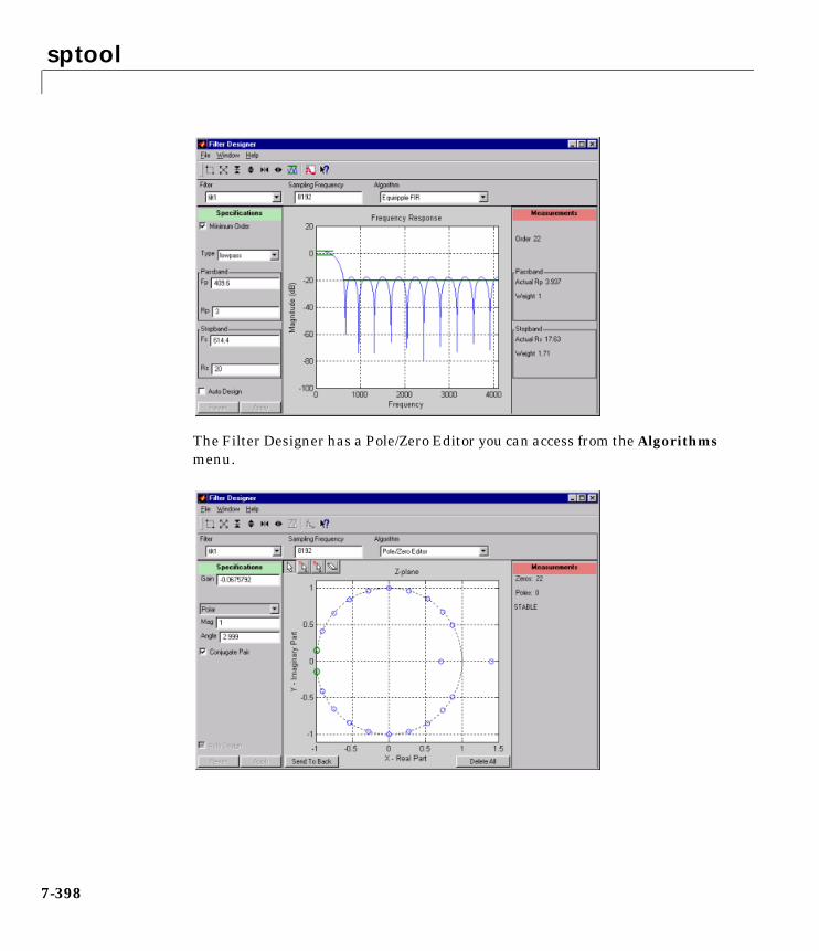
sptool
7-398
The Filter Designer has a Pole/Zero Editor you can access from the Algorithmsmenu.
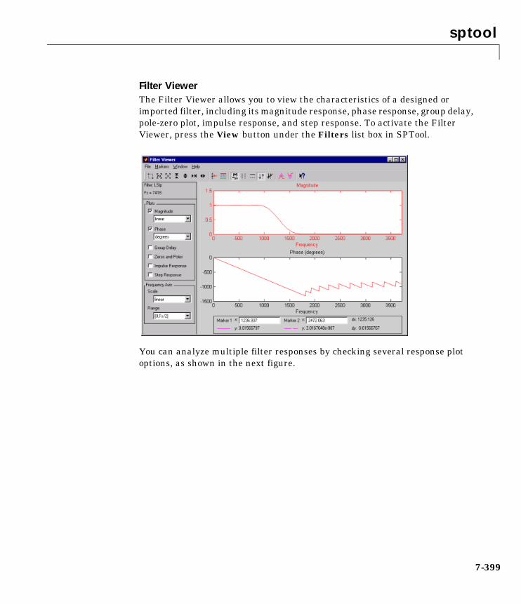
sptool
7-399
Filter ViewerThe Filter Viewer allows you to view the characteristics of a designed orimported filter, including its magnitude response, phase response, group delay,pole-zero plot, impulse response, and step response. To activate the FilterViewer, press the View button under the Filters list box in SPTool.
You can analyze multiple filter responses by checking several response plotoptions, as shown in the next figure.
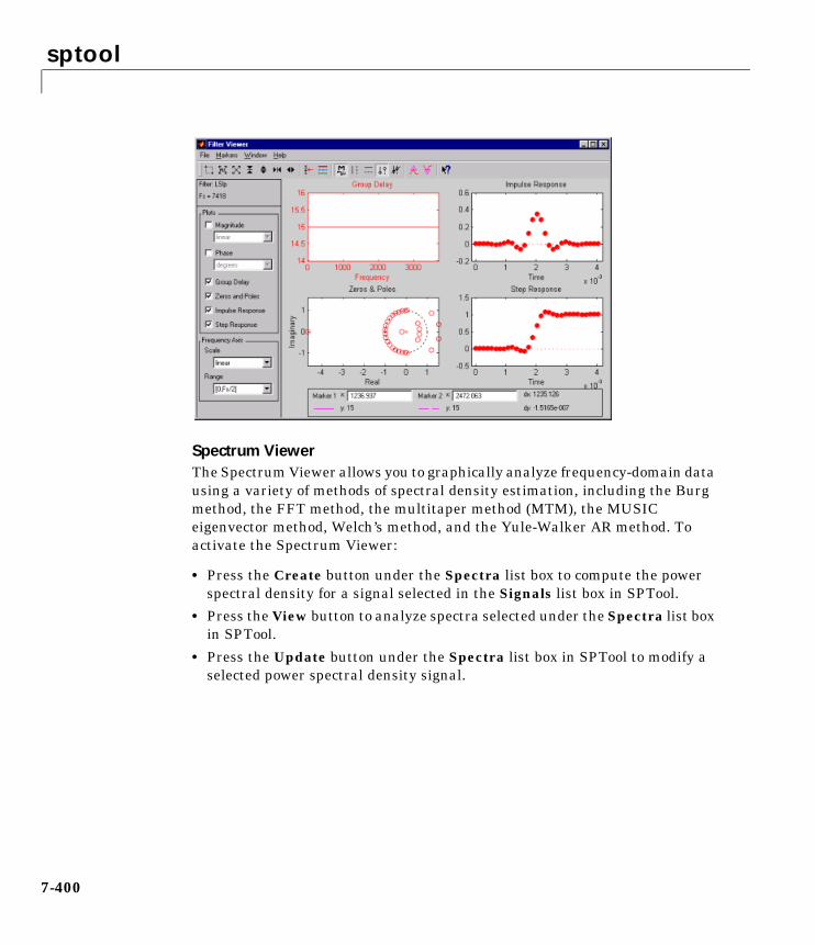
sptool
7-400
Spectrum ViewerThe Spectrum Viewer allows you to graphically analyze frequency-domain datausing a variety of methods of spectral density estimation, including the Burgmethod, the FFT method, the multitaper method (MTM), the MUSICeigenvector method, Welch’s method, and the Yule-Walker AR method. Toactivate the Spectrum Viewer:
• Press the Create button under the Spectra list box to compute the powerspectral density for a signal selected in the Signals list box in SPTool.
• Press the View button to analyze spectra selected under the Spectra list boxin SPTool.
• Press the Update button under the Spectra list box in SPTool to modify aselected power spectral density signal.
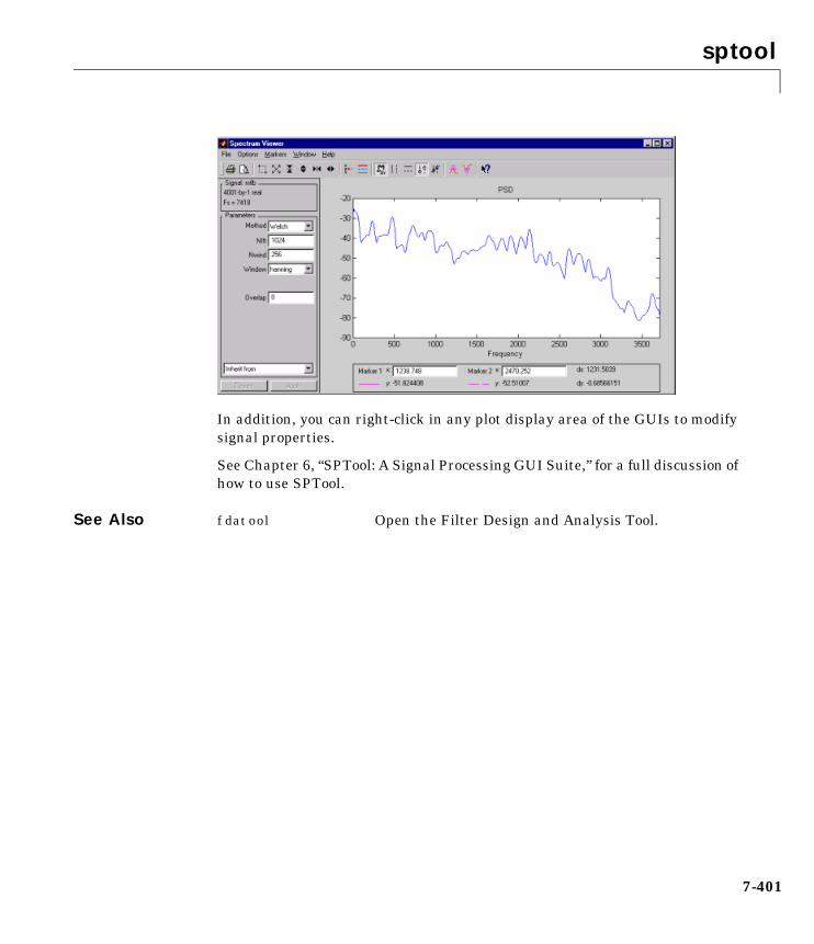
sptool
7-401
In addition, you can right-click in any plot display area of the GUIs to modifysignal properties.
See Chapter 6, “SPTool: A Signal Processing GUI Suite,” for a full discussion ofhow to use SPTool.
See Also fdatool Open the Filter Design and Analysis Tool.

square
7-402
7squarePurpose Generate a square wave.
Syntax x = square(t)x = square(t,duty)
Description x = square(t) generates a square wave with period 2π for the elements oftime vector t. square(t) is similar to sin(t), but creates a square wave withpeaks of ±1 instead of a sine wave.
x = square(t,duty) generates a square wave with specified duty cycle, duty.The duty cycle is the percent of the period in which the signal is positive.
See Also chirp Generate a swept-frequency cosine.
cos Compute the cosine of vector/matrix elements (seethe MATLAB documentation).
diric Compute the Dirichlet or periodic sinc function.
gauspuls Generate a Gaussian-modulated sinusoidal pulse.
pulstran Generate a Pulse train.
rectpuls Generate a sampled aperiodic rectangle.
sawtooth Generate a sawtooth or triangle wave.
sin Compute the sine of vector/matrix elements (see theMATLAB documentation).
sinc Compute the sinc or sin(πt)/πt function.
tripuls Generate a sampled aperiodic triangle.
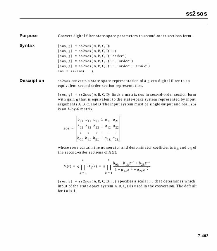
ss2sos
7-403
7ss2sosPurpose Convert digital filter state-space parameters to second-order sections form.
Syntax [sos,g] = ss2sos(A,B,C,D)[sos,g] = ss2sos(A,B,C,D,iu)[sos,g] = ss2sos(A,B,C,D,'order')[sos,g] = ss2sos(A,B,C,D,iu,'order')[sos,g] = ss2sos(A,B,C,D,iu,'order','scale')sos = ss2sos(...)
Description ss2sos converts a state-space representation of a given digital filter to anequivalent second-order section representation.
[sos,g] = ss2sos(A,B,C,D) finds a matrix sos in second-order section formwith gain g that is equivalent to the state-space system represented by inputarguments A, B, C, and D. The input system must be single output and real. sosis an L-by-6 matrix
whose rows contain the numerator and denominator coefficients bik and aik ofthe second-order sections of H(z).
[sos,g] = ss2sos(A,B,C,D,iu) specifies a scalar iu that determines whichinput of the state-space system A, B, C, D is used in the conversion. The defaultfor iu is 1.
sos
b01 b11 b21 1 a11 a21
b02 b12 b22 1 a12 a22
b0L b1L b2L 1 a1L a2L
=
H z( ) g Hk z( )
k 1=
L
∏ gb0k b1kz 1– b2kz 2–+ +
1 a1kz 1– a2kz 2–+ +----------------------------------------------------------
k 1=
L
∏= =
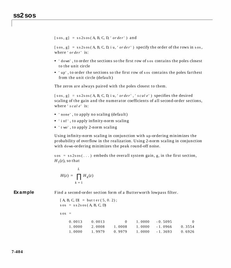
ss2sos
7-404
[sos,g] = ss2sos(A,B,C,D,'order') and
[sos,g] = ss2sos(A,B,C,D,iu,'order') specify the order of the rows in sos,where 'order' is:
• 'down', to order the sections so the first row of sos contains the poles closestto the unit circle
• 'up', to order the sections so the first row of sos contains the poles farthestfrom the unit circle (default)
The zeros are always paired with the poles closest to them.
[sos,g] = ss2sos(A,B,C,D,iu,'order','scale') specifies the desiredscaling of the gain and the numerator coefficients of all second-order sections,where 'scale' is:
• 'none', to apply no scaling (default)
• 'inf', to apply infinity-norm scaling
• 'two', to apply 2-norm scaling
Using infinity-norm scaling in conjunction with up-ordering minimizes theprobability of overflow in the realization. Using 2-norm scaling in conjunctionwith down-ordering minimizes the peak round-off noise.
sos = ss2sos(...) embeds the overall system gain, g, in the first section,H1(z), so that
Example Find a second-order section form of a Butterworth lowpass filter.
[A,B,C,D] = butter(5,0.2);sos = ss2sos(A,B,C,D)
sos =
0.0013 0.0013 0 1.0000 -0.5095 0 1.0000 2.0008 1.0008 1.0000 -1.0966 0.3554 1.0000 1.9979 0.9979 1.0000 -1.3693 0.6926
H z( ) Hk z( )
k 1=
L
∏=

ss2sos
7-405
Algorithm ss2sos uses a four-step algorithm to determine the second-order sectionrepresentation for an input state-space system:
1 It finds the poles and zeros of the system given by A, B, C, and D.
2 It uses the function zp2sos, which first groups the zeros and poles intocomplex conjugate pairs using the cplxpair function. zp2sos then forms thesecond-order sections by matching the pole and zero pairs according to thefollowing rules:
a Match the poles closest to the unit circle with the zeros closest to thosepoles.
b Match the poles next closest to the unit circle with the zeros closest tothose poles.
c Continue until all of the poles and zeros are matched.
ss2sos groups real poles into sections with the real poles closest to them inabsolute value. The same rule holds for real zeros.
3 It orders the sections according to the proximity of the pole pairs to the unitcircle. ss2sos normally orders the sections with poles closest to the unitcircle last in the cascade. You can tell ss2sos to order the sections in thereverse order by specifying the 'down' flag.
4 ss2sos scales the sections by the norm specified in the 'scale' argument.For arbitrary H(ω), the scaling is defined by
where p can be either ∞ or 2. See the references for details. This scaling isan attempt to minimize overflow or peak round-off noise in fixed point filterimplementations.
Diagnostics If there is more than one input to the system, ss2sos gives the following errormessage.
State-space system must have only one input.
H p1
2π------ H ω( ) p ωd
0
2π
1p---
=

ss2sos
7-406
See Also
References [1] Jackson, L.B., Digital Filters and Signal Processing, 3rd ed., KluwerAcademic Publishers, Boston, 1996. Chapter 11.
[2] Mitra, S.K., Digital Signal Processing: A Computer-Based Approach,McGraw-Hill, New York, 1998. Chapter 9.
[3] Vaidyanathan, P.P.,“Robust Digital Filter Structures,” Handbook forDigital Signal Processing, S.K. Mitra and J.F. Kaiser, ed., John Wiley & Sons,New York, 1993, Chapter 7.
cplxpair Group complex numbers into complex conjugatepairs.
sos2ss Convert digital filter second-order sectionsparameters to state-space form.
ss2tf Convert state-space filter parameters to transferfunction form.
ss2zp Convert state-space filter parameters tozero-pole-gain form.
tf2sos Convert digital filter transfer function parameters tosecond-order sections form.
zp2sos Convert digital filter zero-pole-gain parameters tosecond-order sections form.
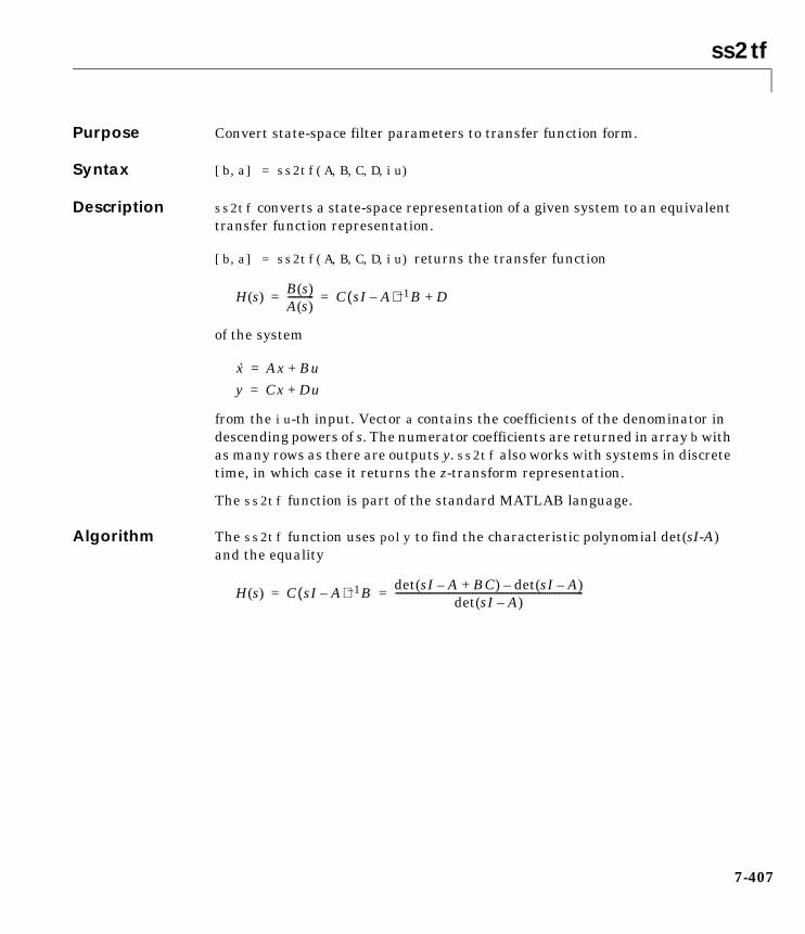
ss2tf
7-407
7ss2tfPurpose Convert state-space filter parameters to transfer function form.
Syntax [b,a] = ss2tf(A,B,C,D,iu)
Description ss2tf converts a state-space representation of a given system to an equivalenttransfer function representation.
[b,a] = ss2tf(A,B,C,D,iu) returns the transfer function
of the system
from the iu-th input. Vector a contains the coefficients of the denominator indescending powers of s. The numerator coefficients are returned in array b withas many rows as there are outputs y. ss2tf also works with systems in discretetime, in which case it returns the z-transform representation.
The ss2tf function is part of the standard MATLAB language.
Algorithm The ss2tf function uses poly to find the characteristic polynomial det(sI-A)and the equality
H s( )B s( )A s( )----------- C sI A–( ) 1– B D+= =
x· Ax Bu+=
y Cx Du+=
H s( ) C sI A–( ) 1– B det sI A– BC+( ) det sI A–( )–det sI A–( )
------------------------------------------------------------------------------= =

ss2tf
7-408
See Also latc2tf Lattice filter to transfer function conversion.
sos2tf Convert digital filter second-order sectionparameters to transfer function form.
ss2sos Convert digital filter state-space parameters tosecond-order sections form.
ss2zp Convert state-space filter parameters tozero-pole-gain form.
tf2ss Convert transfer function filter parameters tostate-space form.
zp2tf Convert zero-pole-gain filter parameters to transferfunction form.

ss2zp
7-409
7ss2zpPurpose Convert state-space filter parameters to zero-pole-gain form.
Syntax [z,p,k] = ss2zp(A,B,C,D,i)
Description ss2zp converts a state-space representation of a given system to an equivalentzero-pole-gain representation. The zeros, poles, and gains of state-spacesystems represent the transfer function in factored form.
[z,p,k] = ss2zp(A,B,C,D,iu) calculates the transfer function in factoredform
of the continuous-time system
from the ith input (using the ith columns of B and D). The column vector pcontains the pole locations of the denominator coefficients of the transferfunction. The matrix z contains the numerator zeros in its columns, with asmany columns as there are outputs y (rows in C). The column vector k containsthe gains for each numerator transfer function.
ss2zp also works for discrete time systems. The input state-space system mustbe real.
The ss2zp function is part of the standard MATLAB language.
Example Here are two ways of finding the zeros, poles, and gains of a discrete-timetransfer function
b = [2 3]; a = [1 0.4 1];[b,a] = eqtflength(b,a);[z,p,k] = tf2zp(b,a)
H s( )Z s( )P s( )---------- k
s z1–( ) s z2–( ) s zn–( )s p1–( ) s p2–( ) s pn–( )
------------------------------------------------------------------= =
x· Ax Bu+=
y Cx Du+=
H z( )2 3z 1–
+
1 0.4z 1– z 2–+ +
-----------------------------------------=

ss2zp
7-410
z = 0.0000 -1.5000
p =-0.2000 + 0.9798i-0.2000 - 0.9798i
k =2
[A,B,C,D] = tf2ss(b,a);[z,p,k] = ss2zp(A,B,C,D,1)
z = 0.0000 -1.5000
p =-0.2000 + 0.9798i-0.2000 - 0.9798i
k =2
Algorithm ss2zp finds the poles from the eigenvalues of the A array. The zeros are thefinite solutions to a generalized eigenvalue problem.
z = eig([A B;C D], diag([ones(1,n) 0]);
In many situations this algorithm produces spurious large, but finite, zeros.ss2zp interprets these large zeros as infinite.
ss2zp finds the gains by solving for the first nonzero Markov parameters.

ss2zp
7-411
See Also
References [1] Laub, A.J., and B.C. Moore, “Calculation of Transmission Zeros Using QZTechniques,” Automatica 14 (1978), p. 557.
pzmap Pole-zero map of LTI system (see the Control SystemToolbox documentation).
sos2zp Convert digital filter second-order section parametersto zero-pole-gain form.
ss2sos Convert digital filter state-space parameters tosecond-order sections form.
ss2tf Convert state-space filter parameters to transferfunction form.
tf2zp Convert transfer function filter parameters tozero-pole-gain form.
zp2ss Convert zero-pole-gain filter parameters tostate-space form.

stmcb
7-412
7stmcbPurpose Compute a linear model using Steiglitz-McBride iteration.
Syntax [b,a] = stmcb(x,nb,na)[b,a] = stmcb(x,u,nb,na)[b,a] = stmcb(x,nb,na,niter)[b,a] = stmcb(x,u,nb,na,niter)[b,a] = stmcb(x,nb,na,niter,ai)[b,a] = stmcb(x,u,nb,na,niter,ai)
Description Steiglitz-McBride iteration is an algorithm for finding an IIR filter with aprescribed time domain impulse response. It has applications in both filterdesign and system identification (parametric modeling).
[b,a] = stmcb(x,nb,na) finds the coefficients b and a of the system b(z)/a(z)with approximate impulse response x, exactly nb zeros, and exactly na poles.
[b,a] = stmcb(x,u,nb,na) finds the system coefficients b and a of the systemthat, given u as input, has x as output. x and u must be the same length.
[b,a] = stmcb(x,nb,na,niter) and
[b,a] = stmcb(x,u,nb,na,niter) use niter iterations. The default for niteris 5.
[b,a] = stmcb(x,nb,na,niter,ai) and
[b,a] = stmcb(x,u,nb,na,niter,ai) use the vector ai as the initial estimateof the denominator coefficients. If ai is not specified, stmcb uses the outputargument from [b,ai] = prony(x,0,na) as the vector ai.
stmcb returns the IIR filter coefficients in length nb+1 and na+1 row vectors band a. The filter coefficients are ordered in descending powers of z.
H z( )B z( )A z( )----------- b 1( ) b 2( )z 1– b nb 1+( )z nb–+ + +
a 1( ) a 2( )z 1– a na 1+( )z na–+ + +--------------------------------------------------------------------------------------------= =

stmcb
7-413
Example Approximate the impulse response of a Butterworth filter with a system oflower order.
[b,a] = butter(6,0.2);h = filter(b,a,[1 zeros(1,100)]);freqz(b,a,128)
[bb,aa] = stmcb(h,4,4);freqz(bb,aa,128)
0 0.1 0.2 0.3 0.4 0.5 0.6 0.7 0.8 0.9 1−600
−500
−400
−300
−200
−100
0
Normalized Frequency (×π rad/sample)
Pha
se (
degr
ees)
0 0.1 0.2 0.3 0.4 0.5 0.6 0.7 0.8 0.9 1−300
−250
−200
−150
−100
−50
0
50
Normalized Frequency (×π rad/sample)
Mag
nitu
de (
dB)
0 0.1 0.2 0.3 0.4 0.5 0.6 0.7 0.8 0.9 1−100
−80
−60
−40
−20
0
20
Normalized Frequency (×π rad/sample)
Pha
se (
degr
ees)
0 0.1 0.2 0.3 0.4 0.5 0.6 0.7 0.8 0.9 1−20
−10
0
10
20
30
40
Normalized Frequency (×π rad/sample)
Mag
nitu
de (
dB)

stmcb
7-414
Algorithm stmcb attempts to minimize the squared error between the impulse response x'of b(z)/a(z) and the input signal x.
stmcb iterates using two steps:
1 It prefilters x and u using 1/a(z).
2 It solves a system of linear equations for b and a using \.
stmcb repeats this process niter times. No checking is done to see if the b and acoefficients have converged in fewer than niter iterations.
Diagnostics If x and u have different lengths, stmcb gives the following error message.
X and U must have same length.
See Also
References [1] Steiglitz, K., and L.E. McBride, “A Technique for the Identification of LinearSystems,” IEEE Trans. Automatic Control, Vol. AC-10 (1965), pp. 461-464.
[2] Ljung, L., System Identification: Theory for the User, Prentice-Hall,Englewood Cliffs, NJ, 1987, p. 297.
mina b,
x i( ) x' i( )– 2
i 0=
∞
levinson Compute the Levinson-Durbin recursion.
lpc Compute linear prediction filter coefficients.
aryule Compute an estimate of AR model parameters usingthe Yule-Walker method.
prony Prony’s method for time domain IIR filter design.

strips
7-415
7stripsPurpose Strip plot.
Syntax strips(x)strips(x,n)strips(x,sd,fs)strips(x,sd,fs,scale)
Description strips(x) plots vector x in horizontal strips of length 250. If x is a matrix,strips(x) plots each column of x. The left-most column (column 1) is the tophorizontal strip.
strips(x,n) plots vector x in strips that are each n samples long.
strips(x,sd,fs) plots vector x in strips of duration sd seconds, given asampling frequency of fs samples per second.
strips(x,sd,fs,scale) scales the vertical axes.
If x is a matrix, strips(x,n), strips(x,sd,fs), and strips(x,sd,fs,scale)plot the different columns of x on the same strip plot.
strips ignores the imaginary part of complex-valued x.
Example Plot two seconds of a frequency modulated sinusoid in 0.25 second strips.
fs = 1000; % Sampling frequencyt = 0:1/fs:2; % Time vectorx = vco(sin(2*pi*t),[10 490],fs); % FM waveformstrips(x,0.25,fs)

strips
7-416
See Also
0 0.05 0.1 0.15 0.2 0.25
1.75
1.5
1.25
1
0.75
0.5
0.25
0
plot Linear two-dimensional plot (see the MATLABdocumentation).
stem Plot discrete sequence data (see the MATLABdocumentation).
tf2latc
7-417
7tf2latcPurpose Convert transfer function filter parameters to lattice filter form.
Syntax [k,v] = tf2latc(b,a)k = tf2latc(1,a)[k,v] = tf2latc(1,a)k = tf2latc(b)
Description [k,v] = tf2latc(b,a) finds the lattice parameters k and the ladderparameters v for an IIR (ARMA) lattice-ladder filter, normalized by a(1). Notethat an error is generated if one or more of the lattice parameters are exactlyequal to 1.
k = tf2latc(1,a) finds the lattice parameters k for an IIR all-pole (AR)lattice filter.
[k,v] = tf2latc(1,a) returns the scalar ladder coefficient at the correctposition in vector v. All other elements of v are zero.
k = tf2latc(b) finds the lattice parameters k for an FIR (MA) lattice filter,normalized by b(1).
See Also latc2tf Convert lattice filter parameters to transfer functionform.
latcfilt Lattice and lattice-ladder filter implementation.
tf2sos Convert transfer function digital filter parameters tosecond-order sections form.
tf2ss Convert transfer function filter parameters tostate-space form.
tf2zp Convert transfer function filter parameters tozero-pole-gain form.
tf2sos
7-418
7tf2sosPurpose Convert digital filter transfer function data to second-order sections form.
Syntax [sos,g] = tf2sos(b,a)[sos,g] = tf2sos(b,a,'order')[sos,g] = tf2sos(b,a,'order','scale')sos = tf2sos(...)
Description tf2sos converts a transfer function representation of a given digital filter to anequivalent second-order section representation.
[sos,g] = tf2sos(b,a) finds a matrix sos in second-order section form withgain g that is equivalent to the digital filter represented by transfer functioncoefficient vectors a and b.
sos is an L-by-6 matrix
whose rows contain the numerator and denominator coefficients bik and aik ofthe second-order sections of H(z).
H z( )B z( )A z( )-----------
b1 b2z 1– bnb 1+ z nb–+ + +
a1 a2z 1– ana 1+ z na–+ + +----------------------------------------------------------------------------= =
sos
b01 b11 b21 1 a11 a21
b02 b12 b22 1 a12 a22
b0L b1L b2L 1 a1L a2L
=
H z( ) g Hk z( )
k 1=
L
∏ gb0k b1kz 1– b2kz 2–+ +
1 a1kz 1– a2kz 2–+ +----------------------------------------------------------
k 1=
L
∏= =
tf2sos
7-419
[sos,g] = tf2sos(b,a,'order') specifies the order of the rows in sos, where'order' is:
• 'down', to order the sections so the first row of sos contains the poles closestto the unit circle
• 'up', to order the sections so the first row of sos contains the poles farthestfrom the unit circle (default)
[sos,g] = tf2sos(b,a,'order','scale') specifies the desired scaling of thegain and numerator coefficients of all second-order sections, where 'scale' is:
• 'none', to apply no scaling (default)
• 'inf', to apply infinity-norm scaling
• 'two', to apply 2-norm scaling
Using infinity-norm scaling in conjunction with up-ordering minimizes theprobability of overflow in the realization. Using 2-norm scaling in conjunctionwith down-ordering minimizes the peak round-off noise.
sos = tf2sos(...) embeds the overall system gain, g, in the first section,H1(z), so that
Algorithm tf2sos uses a four-step algorithm to determine the second-order sectionrepresentation for an input transfer function system:
1 It finds the poles and zeros of the system given by b and a.
2 It uses the function zp2sos, which first groups the zeros and poles intocomplex conjugate pairs using the cplxpair function. zp2sos then forms thesecond-order sections by matching the pole and zero pairs according to thefollowing rules:
a Match the poles closest to the unit circle with the zeros closest to thosepoles.
b Match the poles next closest to the unit circle with the zeros closest tothose poles.
H z( ) Hk z( )
k 1=
L
∏=
tf2sos
7-420
c Continue until all of the poles and zeros are matched.
tf2sos groups real poles into sections with the real poles closest to them inabsolute value. The same rule holds for real zeros.
3 It orders the sections according to the proximity of the pole pairs to the unitcircle. tf2sos normally orders the sections with poles closest to the unitcircle last in the cascade. You can tell tf2sos to order the sections in thereverse order by specifying the 'down' flag.
4 tf2sos scales the sections by the norm specified in the 'scale' argument.For arbitrary H(ω), the scaling is defined by
where p can be either ∞ or 2. See the references for details on the scaling.This scaling is an attempt to minimize overflow or peak round-off noise infixed point filter implementations.
See Also
References [1] Jackson, L.B., Digital Filters and Signal Processing, 3rd ed., KluwerAcademic Publishers, Boston, 1996, Chapter 11.
[2] Mitra, S.K., Digital Signal Processing: A Computer-Based Approach,McGraw-Hill, New York, 1998, Chapter 9.
H p1
2π------ H ω( ) p ωd
0
2π
1p---
=
cplxpair Group complex numbers into complex conjugatepairs.
sos2tf Convert digital filter second-order sectionparameters to transfer function form.
ss2sos Convert digital filter state-space parameters tosecond-order sections form.
tf2ss Convert transfer function filter parameters tostate-space form.
tf2zp Convert transfer function filter parameters tozero-pole-gain form.
zp2sos Convert digital filter zero-pole-gain parameters tosecond-order sections form.

tf2sos
7-421
[3] Vaidyanathan, P.P., “Robust Digital Filter Structures,” Handbook forDigital Signal Processing, S.K. Mitra and J.F. Kaiser, ed., John Wiley & Sons,New York, 1993, Chapter 7.
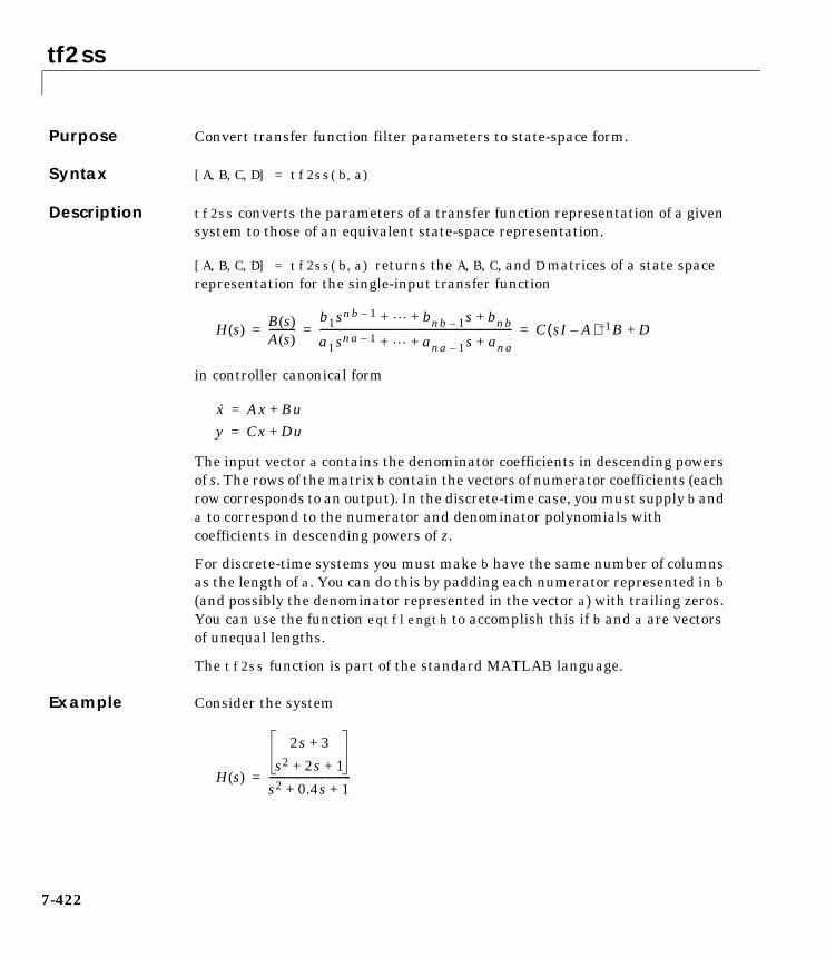
tf2ss
7-422
7tf2ssPurpose Convert transfer function filter parameters to state-space form.
Syntax [A,B,C,D] = tf2ss(b,a)
Description tf2ss converts the parameters of a transfer function representation of a givensystem to those of an equivalent state-space representation.
[A,B,C,D] = tf2ss(b,a) returns the A, B, C, and D matrices of a state spacerepresentation for the single-input transfer function
in controller canonical form
The input vector a contains the denominator coefficients in descending powersof s. The rows of the matrix b contain the vectors of numerator coefficients (eachrow corresponds to an output). In the discrete-time case, you must supply b anda to correspond to the numerator and denominator polynomials withcoefficients in descending powers of z.
For discrete-time systems you must make b have the same number of columnsas the length of a. You can do this by padding each numerator represented in b(and possibly the denominator represented in the vector a) with trailing zeros.You can use the function eqtflength to accomplish this if b and a are vectorsof unequal lengths.
The tf2ss function is part of the standard MATLAB language.
Example Consider the system
H s( )B s( )A s( )-----------
b1snb 1– bnb 1– s bnb+ + +
a1sna 1– ana 1– s ana+ + +------------------------------------------------------------------------------ C sI A–( ) 1– B D+= = =
x· Ax Bu+=
y Cx Du+=
H s( )
2s 3+
s2 2s 1+ +
s2 0.4s 1+ +---------------------------------=
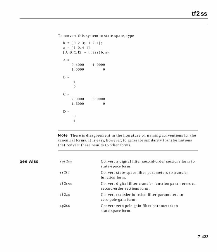
tf2ss
7-423
To convert this system to state-space, type
b = [0 2 3; 1 2 1];a = [1 0.4 1];[A,B,C,D] = tf2ss(b,a)
A = -0.4000 -1.0000 1.0000 0
B = 1 0
C = 2.0000 3.0000 1.6000 0
D = 0 1
Note There is disagreement in the literature on naming conventions for thecanonical forms. It is easy, however, to generate similarity transformationsthat convert these results to other forms.
See Also sos2ss Convert a digital filter second-order sections form tostate-space form.
ss2tf Convert state-space filter parameters to transferfunction form.
tf2sos Convert digital filter transfer function parameters tosecond-order sections form.
tf2zp Convert transfer function filter parameters tozero-pole-gain form.
zp2ss Convert zero-pole-gain filter parameters tostate-space form.
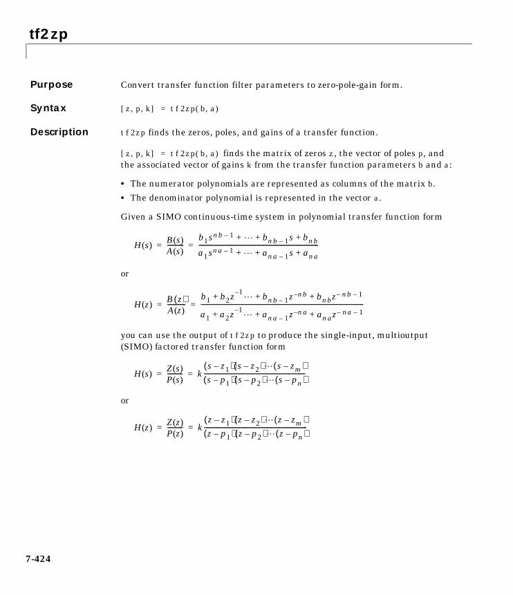
tf2zp
7-424
7tf2zpPurpose Convert transfer function filter parameters to zero-pole-gain form.
Syntax [z,p,k] = tf2zp(b,a)
Description tf2zp finds the zeros, poles, and gains of a transfer function.
[z,p,k] = tf2zp(b,a) finds the matrix of zeros z, the vector of poles p, andthe associated vector of gains k from the transfer function parameters b and a:
• The numerator polynomials are represented as columns of the matrix b.
• The denominator polynomial is represented in the vector a.
Given a SIMO continuous-time system in polynomial transfer function form
or
you can use the output of tf2zp to produce the single-input, multioutput(SIMO) factored transfer function form
or
H s( )B s( )A s( )-----------
b1snb 1– bnb 1– s bnb+ + +
a1sna 1– ana 1– s ana+ + +------------------------------------------------------------------------------= =
H z( )B z( )A z( )------------
b1 b2z 1– bnb 1– z nb– bnbz nb– 1–+ + +
a1 a2z 1– ana 1– z na– anaz na– 1–+ + +
----------------------------------------------------------------------------------------------------------= =
H s( )Z s( )P s( )---------- k
s z1–( ) s z2–( ) s zm–( )s p1–( ) s p2–( ) s pn–( )
------------------------------------------------------------------= =
H z( )Z z( )P z( )---------- k
z z1–( ) z z2–( ) z zm–( )z p1–( ) z p2–( ) z pn–( )
-------------------------------------------------------------------= =
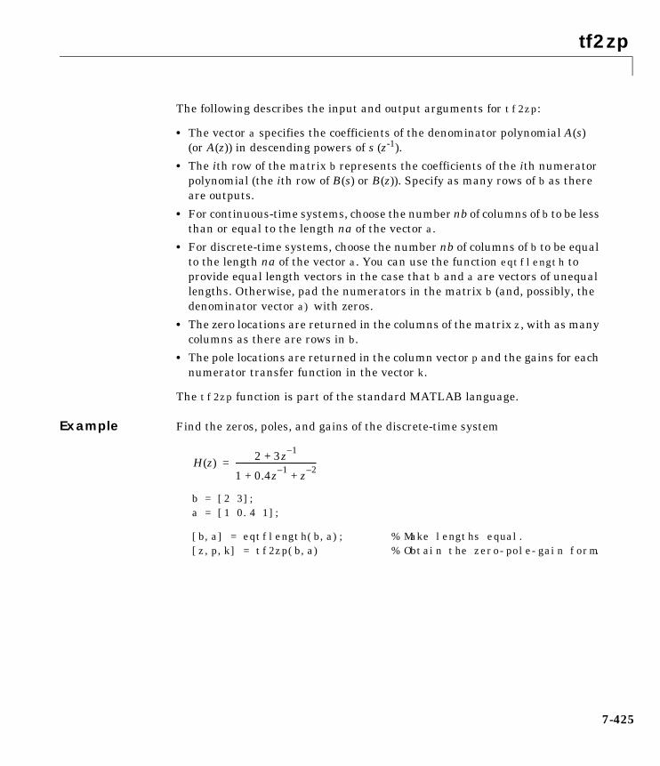
tf2zp
7-425
The following describes the input and output arguments for tf2zp:
• The vector a specifies the coefficients of the denominator polynomial A(s)(or A(z)) in descending powers of s (z-1).
• The ith row of the matrix b represents the coefficients of the ith numeratorpolynomial (the ith row of B(s) or B(z)). Specify as many rows of b as thereare outputs.
• For continuous-time systems, choose the number nb of columns of b to be lessthan or equal to the length na of the vector a.
• For discrete-time systems, choose the number nb of columns of b to be equalto the length na of the vector a. You can use the function eqtflength toprovide equal length vectors in the case that b and a are vectors of unequallengths. Otherwise, pad the numerators in the matrix b (and, possibly, thedenominator vector a) with zeros.
• The zero locations are returned in the columns of the matrix z, with as manycolumns as there are rows in b.
• The pole locations are returned in the column vector p and the gains for eachnumerator transfer function in the vector k.
The tf2zp function is part of the standard MATLAB language.
Example Find the zeros, poles, and gains of the discrete-time system
b = [2 3];a = [1 0.4 1];
[b,a] = eqtflength(b,a); % Make lengths equal.[z,p,k] = tf2zp(b,a) % Obtain the zero-pole-gain form.
H z( )2 3z 1–
+
1 0.4z 1– z 2–+ +
-----------------------------------------=
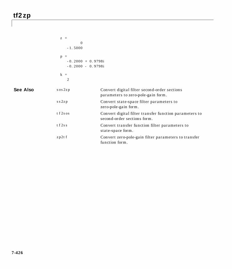
tf2zp
7-426
z = 0 -1.5000
p = -0.2000 + 0.9798i -0.2000 - 0.9798i
k = 2
See Also sos2zp Convert digital filter second-order sectionsparameters to zero-pole-gain form.
ss2zp Convert state-space filter parameters tozero-pole-gain form.
tf2sos Convert digital filter transfer function parameters tosecond-order sections form.
tf2ss Convert transfer function filter parameters tostate-space form.
zp2tf Convert zero-pole-gain filter parameters to transferfunction form.
tfe
7-427
7tfePurpose Estimate the transfer function from input and output.
Syntax Txy = tfe(x,y)Txy = tfe(x,y,nfft)[Txy,f] = tfe(x,y,nfft,fs)Txy = tfe(x,y,nfft,fs,window)Txy = tfe(x,y,nfft,fs,window,numoverlap)Txy = tfe(x,y,...,'dflag')tfe(x,y)
Description Txy = tfe(x,y) finds a transfer function estimate Txy given input signalvector x and output signal vector y. The transfer function is the quotient of thecross spectrum of x and y and the power spectrum of x.
The relationship between the input x and output y is modeled by the linear,time-invariant transfer function Txy.
Vectors x and y must be the same length. Txy = tfe(x,y) uses the followingdefault values:
• nfft = min(256,(length(x))
• fs = 2
• window is a periodic Hann (Hanning) window of length nfft
• numoverlap = 0
nfft specifies the FFT length that tfe uses. This value determines thefrequencies at which the power spectrum is estimated. fs is a scalar thatspecifies the sampling frequency. window specifies a windowing function andthe number of samples tfe uses in its sectioning of the x and y vectors.numoverlap is the number of samples by which the sections overlap. Anyarguments that are omitted from the end of the parameter list use the defaultvalues shown above.
If x is real, tfe estimates the transfer function at positive frequencies only; inthis case, the output Txy is a column vector of length nfft/2+1 for nfft evenand (nfft+1)/2 for nfft odd. If x or y is complex, tfe estimates the transferfunction for both positive and negative frequencies and Txy has length nfft.
Txy f( )Pxy f( )
Pxx f( )---------------=
tfe
7-428
Txy = tfe(x,y,nfft) uses the specified FFT length nfft in estimating thetransfer function.
[Txy,f] = tfe(x,y,nfft,fs) returns a vector f of frequencies at which tfeestimates the transfer function. fs is the sampling frequency. f is the same sizeas Txy, so plot(f,Txy) plots the transfer function estimate versus properlyscaled frequency. fs has no effect on the output Txy; it is a frequency scalingmultiplier.
Txy = tfe(x,y,nfft,fs,window) specifies a windowing function and thenumber of samples per section of the x vector. If you supply a scalar for window,Txy uses a Hann window of that length. The length of the window must be lessthan or equal to nfft; tfe zero pads the sections if the length of the windowexceeds nfft.
Txy = tfe(x,y,nfft,fs,window,numoverlap) overlaps the sections of x bynumoverlap samples.
You can use the empty matrix [] to specify the default value for any inputargument except x or y. For example,
Txy = tfe(x,y,[],[],kaiser(128,5))
uses 256 as the value for nfft and 2 as the value for fs.
Txy = tfe(x,y,...,'dflag') specifies a detrend option, where 'dflag' is:
• 'linear', to remove the best straight-line fit from the prewindowed sectionsof x and y
• 'mean', to remove the mean from the prewindowed sections of x and y
• 'none', for no detrending (default)
The 'dflag' parameter must appear last in the list of input arguments. tferecognizes a 'dflag' string no matter how many intermediate arguments areomitted.
tfe(...) with no output arguments plots the magnitude of the transferfunction estimate as decibels versus frequency in the current figure window.
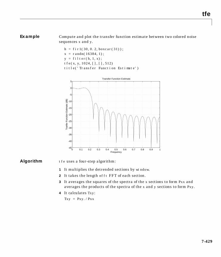
tfe
7-429
Example Compute and plot the transfer function estimate between two colored noisesequences x and y.
h = fir1(30,0.2,boxcar(31));x = randn(16384,1);y = filter(h,1,x);tfe(x,y,1024,[],[],512)title('Transfer Function Estimate')
Algorithm tfe uses a four-step algorithm:
1 It multiplies the detrended sections by window.
2 It takes the length nfft FFT of each section.
3 It averages the squares of the spectra of the x sections to form Pxx andaverages the products of the spectra of the x and y sections to form Pxy.
4 It calculates Txy:Txy = Pxy./Pxx
0 0.1 0.2 0.3 0.4 0.5 0.6 0.7 0.8 0.9 1-45
-40
-35
-30
-25
-20
-15
-10
-5
0
5
Frequency
Tra
nfer
Fun
ctio
n E
stim
ate
(dB
)
Transfer Function Estimate
tfe
7-430
Diagnostics An appropriate diagnostic message is displayed when incorrect arguments areused.
Requires window's length to be no greater than the FFT length.Requires NOVERLAP to be strictly less than the window length.Requires positive integer values for NFFT and NOVERLAP.Requires vector (either row or column) input.Requires inputs X and Y to have the same length.
See Also etfe Compute empirical transfer function estimate andperiodogram (see the System Identification Toolboxdocumentation).
cohere Estimate magnitude squared coherence functionbetween two signals.
csd Estimate the cross spectral density (CSD) of twosignals.
pwelch Estimate the power spectral density (PSD) of a signalusing Welch’s method.
spa Perform spectral analysis for input-output data (seethe System Identification Toolbox documentation).

triang
7-431
7triangPurpose Compute a triangular window.
Syntax w = triang(n)
Description triang(n) returns an n-point triangular window in the column vector w. Thecoefficients of a triangular window are
For n odd:
For n even:
The triangular window is very similar to a Bartlett window. The Bartlettwindow always ends with zeros at samples 1 and n, while the triangularwindow is nonzero at those points. For n odd, the center n-2 points oftriang(n-2) are equivalent to bartlett(n).
Example w = triang(200);plot(w)title('Triangular Window')
w k[ ]
2kn 1+------------- 1 k n 1+
2-------------≤ ≤,
2 n k 1+–( )n 1+
------------------------------- n 1+2
------------- k n≤ ≤,
=
w k[ ]
2k 1–n
---------------- 1 k n2---≤ ≤,
2 n k 1+–( )n
------------------------------- n2--- 1+ k n≤ ≤,
=
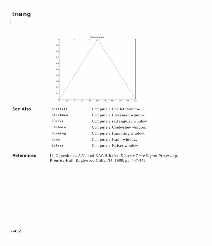
triang
7-432
See Also
References [1] Oppenheim, A.V., and R.W. Schafer, Discrete-Time Signal Processing,Prentice-Hall, Englewood Cliffs, NJ, 1989, pp. 447-448.
0 20 40 60 80 100 120 140 160 180 2000
0.1
0.2
0.3
0.4
0.5
0.6
0.7
0.8
0.9
1Triangular Window
bartlett Compute a Bartlett window.
blackman Compute a Blackman window.
boxcar Compute a rectangular window.
chebwin Compute a Chebyshev window.
hamming Compute a Hamming window.
hann Compute a Hann window.
kaiser Compute a Kaiser window.
tripuls
7-433
7tripulsPurpose Generate a sampled aperiodic triangle.
Syntax y = tripuls(T)y = tripuls(T,w)y = tripuls(T,w,s)
Description y = tripuls(T) returns a continuous, aperiodic, symmetric, unity-heighttriangular pulse at the times indicated in array T, centered about T=0 and witha default width of 1.
y = tripuls(T,w) generates a triangular pulse of width w.
y = tripuls(T,w,s) generates a triangular pulse with skew s, where-1 < s < 1. When s is 0, a symmetric triangular pulse is generated.
See Also chirp Generate a swept-frequency cosine.
cos Compute the cosine of vector/matrix elements (see theMATLAB documentation).
diric Compute the Dirichlet or periodic sinc function.
gauspuls Generate a Gaussian-modulated sinusoidal pulse.
pulstran Generate a pulse train.
rectpuls Generate a sampled aperiodic rectangle.
sawtooth Generate a sawtooth or triangle wave.
sin Compute the sine of vector/matrix elements (see theMATLAB documentation).
sinc Compute the sinc or sin(πt)/πt function.
square Generate a square wave.
udecode
7-434
7udecodePurpose Decode 2n-level quantized integer inputs to floating-point outputs.
Syntax y = udecode(u,n)y = udecode(u,n,v)y = udecode(u,n,v,'saturatemode')
Description y = udecode(u,n) inverts the operation of uencode and reconstructsquantized floating-point values from an encoded multidimensional array ofintegers u. The input argument n must be an integer between 2 and 32. Theinteger n specifies that there are 2n quantization levels for the inputs, so thatentries in u must be either:
• Signed integers in the range [-2n/2, (2n/2) - 1]
• Unsigned integers in the range [0, 2n-1]
Inputs can be real or complex values of any integer data type (uint8, uint16,uint32, int8, int16, int32). Overflows (entries in u outside of the rangesspecified above) are saturated to the endpoints of the range interval. Theoutput y has the same dimensions as u. Its entries have values in the range[-1,1].
y = udecode(u,n,v) decodes u such that the output y has values in the range[-v,v], where the default value for v is 1.
y = udecode(u,n,v,'SaturateMode') decodes u and treats input overflows(entries in u outside of [-v,v]) according to the string 'saturatemode', whichcan be one of the following:
• 'saturate': Saturate overflows. This is the default method for treatingoverflows.- Entries in signed inputs u whose values are outside of the range
[-2n/2, (2n/2) - 1] are assigned the value determined by the closest endpointof this interval.
- Entries in unsigned inputs u whose values are outside of the range[0, 2n-1] are assigned the value determined by the closest endpoint of thisinterval.
udecode
7-435
• 'wrap': Wrap all overflows according to the following:
- Entries in signed inputs u whose values are outside of the range[-2n/2, (2n/2) - 1] are wrapped back into that range using modulo 2n
arithmetic (calculated using u = mod(u+2^n/2,2^n)-(2^n/2)).
- Entries in unsigned inputs u whose values are outside of the range[0, 2n-1] are wrapped back into the required range before decoding usingmodulo 2n arithmetic (calculated using u = mod(u,2^n)).
Examples u = int8([-1 1 2 -5]); % Create a signed 8-bit integer string.ysat = udecode(u,3) % Decode with 3 bits.ysat =
-0.2500 0.2500 0.5000 -1.0000
Notice the last entry in u saturates to 1, the default peak input magnitude.Change the peak input magnitude.
ysatv = udecode(u,3,6) % Set the peak input magnitude to 6.ysatv =
-1.5000 1.5000 3.0000 -6.0000
The last input entry still saturates. Try wrapping the overflows.
ywrap = udecode(u,3,6,'wrap')ywrap =
-1.5000 1.5000 3.0000 4.5000
Try adding more quantization levels.
yprec = udecode(u,5)yprec =
-0.0625 0.0625 0.1250 -0.3125
Algorithm The algorithm adheres to the definition for uniform decoding specified in ITU-TRecommendation G.701. Integer input values are uniquely mapped (decoded)from one of 2n uniformly spaced integer values to quantized floating-pointvalues in the range [-v,v]. The smallest integer input value allowed ismapped to -v and the largest integer input value allowed is mapped to v.

udecode
7-436
Values outside of the allowable input range are either saturated or wrapped,according to specification.
The real and imaginary components of complex inputs are decodedindependently.
See Also uencode Quantize and encode floating-point data.
References General Aspects of Digital Transmission Systems: Vocabulary of DigitalTransmission and Multiplexing, and Pulse Code Modulation (PCM) Terms,International Telecommunication Union, ITU-T Recommendation G.701,March, 1993.
uencode
7-437
7uencodePurpose Quantize and encode floating-point inputs to integer outputs.
Syntax y = uencode(u,n)y = uencode(u,n,v)y = uencode(u,n,v,'SignFlag')
Description y = uencode(u,n) quantizes the entries in a multidimensional array offloating-point numbers u and encodes them as integers using 2n-levelquantization. n must be an integer between 2 and 32 (inclusive). Inputs can bereal or complex, double- or single-precision. The output y and the input u arearrays of the same size. The elements of the output y are unsigned integerswith magnitudes in the range [0, 2n-1]. Elements of the input u outside of therange [-1,1] are treated as overflows and are saturated.
• For entries in the input u that are less than -1, the value of the output ofuencode is 0.
• For entries in the input u that are greater than 1, the value of the output ofuencode is 2n-1.
y = uencode(u,n,v) allows the input u to have entries with floating-pointvalues in the range [-v,v] before saturating them (the default value for v is 1).Elements of the input u outside of the range [-v,v] are treated as overflowsand are saturated.
• For input entries less than -v, the value of the output of uencode is 0.
• For input entries greater than v, the value of the output of uencode is 2n-1.
y = uencode(u,n,v,'SignFlag') maps entries in a multidimensional array offloating-point numbers u whose entries have values in the range [-v,v] to aninteger output y. Input entries outside this range are saturated. The integertype of the output depends on the string 'SignFlag' and the number ofquantization levels 2n. The string 'SignFlag' can be one of the following:
• 'signed': Outputs are signed integers with magnitudes in the range[-2n/2, (2n/2) - 1].
• 'unsigned' (default): Outputs are unsigned integers with magnitudes in therange [0, 2n-1].
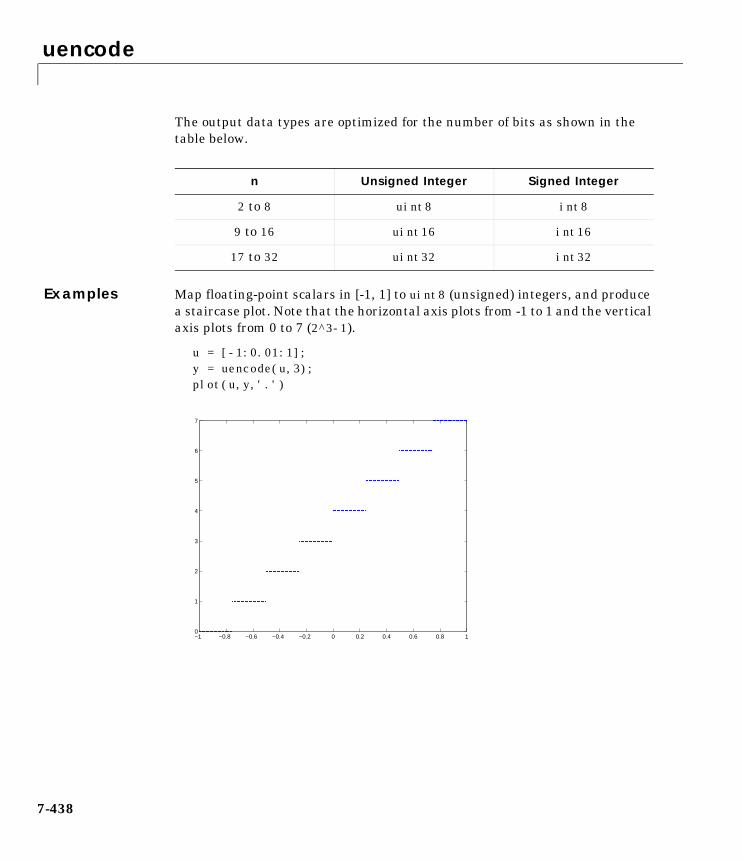
uencode
7-438
The output data types are optimized for the number of bits as shown in thetable below.
Examples Map floating-point scalars in [-1, 1] to uint8 (unsigned) integers, and producea staircase plot. Note that the horizontal axis plots from -1 to 1 and the verticalaxis plots from 0 to 7 (2^3-1).
u = [-1:0.01:1];y = uencode(u,3);plot(u,y,'.')
n Unsigned Integer Signed Integer
2 to 8 uint8 int8
9 to 16 uint16 int16
17 to 32 uint32 int32
−1 −0.8 −0.6 −0.4 −0.2 0 0.2 0.4 0.6 0.8 10
1
2
3
4
5
6
7
uencode
7-439
Now look at saturation effects when you under specify the peak value for theinput.
u = [-2:0.5:2];y = uencode(u,5,1)
y = 0 0 0 8 16 24 31 31 31
Now look at the output for
u = [-2:0.5:2];y = uencode(u,5,2,'signed')
y = -8 -4 0 4 8 12 16 20 23
Algorithm uencode maps the floating-point input value to an integer value determined bythe requirement for 2n levels of quantization. This encoding adheres to thedefinition for uniform encoding specified in ITU-T Recommendation G.701.The input range [-v,v] is divided into 2n evenly spaced intervals. Inputentries in the range [-v,v] are first quantized according to this subdivision ofthe input range, and then mapped to one of 2n integers. The range of the outputdepends on whether or not you specify that you want signed integers.
See Also udecode Decode 2n-level quantized integers to floating-point.
References General Aspects of Digital Transmission Systems: Vocabulary of DigitalTransmission and Multiplexing, and Pulse Code Modulation (PCM) Terms,International Telecommunication Union, ITU-T Recommendation G.701,March, 1993.

unwrap
7-440
7unwrapPurpose Unwrap phase angles.
Syntax p = unwrap(p)
Description p = unwrap(p) corrects the phase angles in vector p by adding multiples of, where needed, to smooth the transitions across branch cuts. When p is a
matrix, unwrap corrects the phase angles down each column. The phase mustbe in radians.
The unwrap function is part of the standard MATLAB language.
Limitations unwrap tries to detect branch cut crossings, but it can be fooled by sparse,rapidly changing phase values.
See Also
2π±
abs Absolute value (magnitude).
angle Phase angle.
upfirdn
7-441
7upfirdnPurpose Upsample, apply an FIR filter, and downsample.
Syntax yout = upfirdn(xin,h)yout = upfirdn(xin,h,p)yout = upfirdn(xin,h,p,q)[yout,zf] = upfirdn(xin,h,...,zi)
Description upfirdn performs a cascade of three operations:
1 Upsampling the input data in the matrix xin by a factor of the integer p(inserting zeros)
2 FIR filtering the upsampled signal data with the impulse response sequencegiven in the vector or matrix h
3 Downsampling the result by a factor of the integer q (throwing awaysamples)
upfirdn has been implemented as a MEX-file for maximum speed, so only theoutputs actually needed are computed. The FIR filter is usually a lowpassfilter, which you must design using another function such as remez or fir1.
Note The function resample performs an FIR design using firls, followedby rate changing implemented with upfirdn.
yout = upfirdn(xin,h) filters the input signal xin with the FIR filter havingimpulse response h. If xin is a row or column vector, then it represents a singlesignal. If xin is a matrix, then each column is filtered independently. If h is arow or column vector, then it represents one FIR filter. If h is a matrix, theneach column is a separate FIR impulse response sequence. If yout is a row orcolumn vector, then it represents one signal. If yout is a matrix, then eachcolumn is a separate output. No upsampling or downsampling is implementedwith this syntax.
yout = upfirdn(xin,h,p) specifies the integer upsampling factor p, where phas a default value of 1.
upfirdn
7-442
yout = upfirdn(xin,h,p,q) specifies the integer downsampling factor q,where q has a default value of 1.
[yout,zf] = upfirdn(xin,h,...,zi) specifies initial state conditions in thevector zi.
The size of the initial condition vector zimust be the same as length(h)-1, thenumber of delays in the FIR filter.
When xin is a vector, the size of the final condition vector zf is length(h)-1,the number of delays in the filter. When xin is a matrix, zf is an matrix with(length(h)-1) rows and (size(xin,2)) columns.
Note Since upfirdn performs convolution and rate changing, the youtsignals have a different length than xin. The number of rows of yout isapproximately p/q times the number of rows of xin.
Remarks Usually the inputs xin and the filter h are vectors, in which case only oneoutput signal is produced. However, when these arguments are arrays, eachcolumn is treated as a separate signal or filter. Valid combinations are:
1 xin is a vector and h is a vector.
There is one filter and one signal, so the function convolves xin with h. Theoutput signal yout is a row vector if xin is a row; otherwise, yout is a columnvector.
2 xin is a matrix and h is a vector.
There is one filter and many signals, so the function convolves h with eachcolumn of xin. The resulting yout will be an matrix with the same numberof columns as xin.
3 xin is a vector and h is a matrix.
There are many filters and one signal, so the function convolves each columnof h with xin. The resulting yout will be an matrix with the same number ofcolumns as h.
upfirdn
7-443
4 xin is a matrix and h is a matrix, both with the same number of columns.
There are many filters and many signals, so the function convolvescorresponding columns of xin and h. The resulting yout is an matrix withthe same number of columns as xin and h.
Examples If both p and q are equal to 1 (that is, there is no rate changing), the result isordinary convolution of two signals (equivalent to conv).
yy = upfirdn(xx,hh);
This example implements a seven-channel filter bank by convolving sevendifferent filters with one input signal, then downsamples by five.
% Assume that hh is an L-by-7 array of filters.yy = upfirdn(xx,hh,1,5);
Implement a rate change from 44.1 kHz (CD sampling rate) to 48 kHz (DATrate), a ratio of 160/147. This requires a lowpass filter with cutoff frequency atωc = 2π/160.
% Design lowpass filter with cutoff at 1/160th of fs.
hh = fir1(300,2/160); % Need a very long lowpass filteryy = upfirdn(xx,hh,160,147);
In this example, the filter design and resampling are separate steps. Note thatresample would do both steps as one.
Algorithm upfirdn uses a polyphase interpolation structure. The number of multiply-addoperations in the polyphase structure is approximately (LhLx-pLx)/q where Lhand Lx are the lengths of h[n] and x[n], respectively.
A more accurate flops count is computed in the program, but the actual countis still approximate. For long signals x[n], the formula is quite often exact.
upfirdn
7-444
See Also
References [1] Crochiere, R.E., and L.R. Rabiner, Multi-Rate Signal Processing,Prentice-Hall, Englewood Cliffs, NJ, 1983, pp. 88-91.
[2] Crochiere, R.E., “A General Program to Perform Sampling Rate Conversionof Data by Rational Ratios,” Programs for Digital Signal Processing, IEEEPress, New York, 1979, pp. 8.2-1 to 8.2-7.
conv Convolution and polynomial multiplication.
decimate Decrease the sampling rate for a sequence(decimation).
filter Filter data with a recursive (IIR) or nonrecursive(FIR) filter.
interp Increase sampling rate by an integer factor(interpolation).
intfilt Interpolation FIR filter design.
resample Change sampling rate by any rational factor.
vco
7-445
7vcoPurpose Voltage controlled oscillator.
Syntax y = vco(x,fc,fs)y = vco(x,[Fmin Fmax],fs)
Description y = vco(x,fc,fs) creates a signal that oscillates at a frequency determinedby the real input vector or array x with sampling frequency fs. fc is the carrieror reference frequency; when x is 0, y is an fc Hz cosine with amplitude 1sampled at fs Hz. x ranges from -1 to 1, where x = -1 corresponds to0 frequency output, x = 0 corresponds to fc, and x = 1 corresponds to 2*fc.Output y is the same size as x.
y = vco(x,[Fmin Fmax],fs) scales the frequency modulation range so that±1 values of x yield oscillations of Fmin Hz and Fmax Hz respectively. For bestresults, Fmin and Fmax should be in the range 0 to fs/2.
By default, fs is 1 and fc is fs/4.
If x is a matrix, vco produces a matrix whose columns oscillate according to thecolumns of x.
Example Generate two seconds of a signal sampled at 10,000 samples/second whoseinstantaneous frequency is a triangle function of time.
fs = 10000;t = 0:1/fs:2;x = vco(sawtooth(2*pi*t,0.75),[0.1 0.4]*fs,fs);
Plot the spectrogram of the generated signal.
specgram(x,512,fs,kaiser(256,5),220)
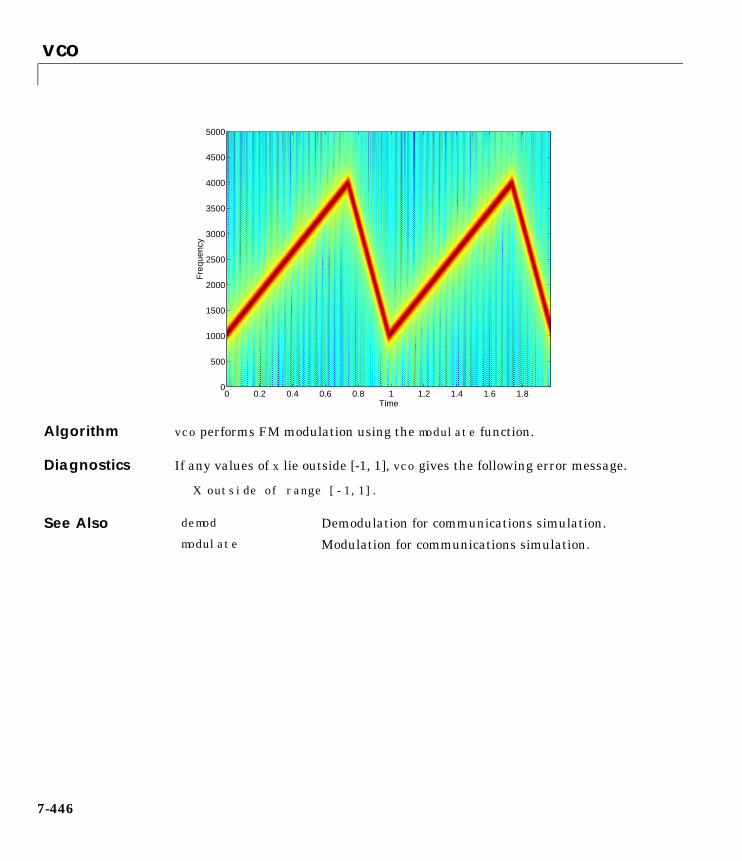
vco
7-446
Algorithm vco performs FM modulation using the modulate function.
Diagnostics If any values of x lie outside [-1, 1], vco gives the following error message.
X outside of range [-1,1].
See Also
Time
Fre
quen
cy
0 0.2 0.4 0.6 0.8 1 1.2 1.4 1.6 1.80
500
1000
1500
2000
2500
3000
3500
4000
4500
5000
demod Demodulation for communications simulation.
modulate Modulation for communications simulation.
xcorr
7-447
7xcorrPurpose Estimate the cross-correlation function.
Syntax c = xcorr(x,y)c = xcorr(x)c = xcorr(x,y,'option')c = xcorr(x,'option')c = xcorr(x,y,maxlags)c = xcorr(x,maxlags)c = xcorr(x,y,maxlags,'option')c = xcorr(x,maxlags,'option')[c,lags] = xcorr(...)
Description xcorr estimates the cross-correlation sequence of a random process.Autocorrelation is handled as a special case.
The true cross-correlation sequence is
where xn and yn are jointly stationary random processes, , and E ·is the expected value operator. xcorr must estimate the sequence because, inpractice, only a finite segment of one realization of the infinite-length randomprocess is available.
c = xcorr(x,y) returns the cross-correlation sequence in a length 2*N-1vector, where x and y are length N vectors (N>1). If x and y are not the samelength, the shorter vector is zero-padded to the length of the longer vector.
By default, xcorr computes raw correlations with no normalization.
The output vector c has elements given by c(m) = cxy(m-N), m=1, ..., 2N-1.
In general, the correlation function requires normalization to produce anaccurate estimate (see below).
Rxy m( ) Exn m+ y*n Exny*n m– ==
∞– n ∞< <
Rˆ
xy m( )xn m+ yn
*
n 0=
N m– 1–
m 0≥
Rˆ
yx*
m–( ) m 0<
=

xcorr
7-448
c = xcorr(x) is the autocorrelation sequence for the vector x. If x is an N-by-Pmatrix, c is a matrix with 2N-1 rows whose P2 columns contain thecross-correlation sequences for all combinations of the columns of x.
c = xcorr(x,y,'option') specifies a normalization option for thecross-correlation, where 'option' is:
• 'biased': Biased estimate of the cross-correlation function
• 'unbiased': Unbiased estimate of the cross-correlation function
• 'coeff': Normalizes the sequence so the autocorrelations at zero lag areidentically 1.0
• 'none', to use the raw, unscaled cross-correlations (default)
See reference [1] for more information on the properties of biased and unbiasedcorrelation estimates.
c = xcorr(x,'option') specifies one of the above normalization options forthe autocorrelation.
c = xcorr(x,y,maxlags) returns the cross-correlation sequence over the lagrange [-maxlags:maxlags]. Output c has length 2*maxlags+1.
c = xcorr(x,maxlags) returns the autocorrelation sequence over the lagrange [-maxlags:maxlags]. Output c has length 2*maxlags+1. If x is anN-by-P matrix, c is a matrix with 2*maxlags+1 rows whose P2 columns containthe autocorrelation sequences for all combinations of the columns of x.
c = xcorr(x,y,maxlags,'option') specifies both a maximum number of lagsand a scaling option for the cross-correlation.
c = xcorr(x,maxlags,'option') specifies both a maximum number of lagsand a scaling option for the autocorrelation.
cxy biased, m( )1N----cxy m( )=
cxy unbiased, m( )1
N m–-------------------cxy m( )=
xcorr
7-449
[c,lags] = xcorr(...) returns a vector of the lag indices at which c wasestimated, with the range [-maxlags:maxlags]. When maxlags is notspecified, the range of lags is [-N+1:N-1].
In all cases, the cross-correlation or autocorrelation computed by xcorr has thezeroth lag in the middle of the sequence, at element or row maxlags+1 (elementor row N if maxlags is not specified).
Examples The second output, lags, is useful for plotting the cross-correlation orautocorrelation. For example, the estimated autocorrelation of zero-meanGaussian white noise cww(m) can be displayed for -10 ≤ m ≤ 10 using
ww = randn(1000,1);[c_ww,lags] = xcorr(ww,10,'coeff');stem(lags,c_ww)
Swapping the x and y input arguments reverses (and conjugates) the outputcorrelation sequence. For row vectors, the resulting sequences are reversed leftto right; for column vectors, up and down. The following example illustratesthis property (mat2str is used for a compact display of complex numbers).
x = [1,2i,3]; y = [4,5,6];[c1,lags] = xcorr(x,y);c1 = mat2str(c1,2), lagsc1 =
[6-i*8.9e-016 5+i*12 22+i*10 15+i*8 12+i*8.9e-016]lags = -2 -1 0 1 2c2 = conj(fliplr(xcorr(y,x)));c2 = mat2str(c2,2)c2 =
[6-i*8.9e-016 5+i*12 22+i*10 15+i*8 12+i*8.9e-016]
For the case where input argument x is a matrix, the output columns arearranged so that extracting a row and rearranging it into a square arrayproduces the cross-correlation matrix corresponding to the lag of the chosenrow. For example, the cross-correlation at zero lag can be retrieved by
randn('state',0)X = randn(2,2);[M,P] = size(X);c = xcorr(X);

xcorr
7-450
c0 = zeros(P); c0(:) = c(M,:) % Extract zero-lag row
c0 = 2.9613 -0.5334 -0.5334 0.0985
You can calculate the matrix of correlation coefficients that the MATLABfunction corrcoef generates by substituting
c = xcov(X,'coef')
in the last example. The function xcov subtracts the mean and then callsxcorr.
Use fftshift to move the second half of the sequence starting at the zeroth lagto the front of the sequence. fftshift swaps the first and second halves of asequence.
Algorithm For more information on estimating covariance and correlation functions, see[1].
See Also
References [1] Orfanidis, S.J., Optimum Signal Processing. An Introduction. 2nd Edition,Prentice-Hall, Englewood Cliffs, NJ, 1996.
conv Convolution and polynomial multiplication.
corrcoef Compute a correlation coefficient matrix.
cov Compute a covariance matrix.
xcorr2 Estimate the two-dimensional cross-correlation.
xcov Estimate the cross-covariance.

xcorr2
7-451
7xcorr2Purpose Estimate the two-dimensional cross-correlation.
Syntax C = xcorr2(A)C = xcorr2(A,B)
Description C = xcorr2(A,B) returns the cross-correlation of matrices A and B with noscaling. xcorr2 is the two-dimensional version of xcorr. It has its maximumvalue when the two matrices are aligned so that they are shaped as similarlyas possible.
xcorr2(A) is the autocorrelation matrix of input matrix A. It is identical toxcorr2(A,A).
See Also conv2 Compute the two-dimensional convolution.
filter2 Filter two-dimensional data.
xcorr Estimate the cross-correlation function.

xcov
7-452
7xcovPurpose Estimate the cross-covariance function (mean-removed cross-correlation).
Syntax v = xcov(x,y)v = xcov(x)v = xcov(x,'option')[c,lags] = xcov(x,y,maxlags)[c,lags] = xcov(x,maxlags)[c,lags] = xcov(x,y,maxlags,'option')
Description xcov estimates the cross-covariance sequence of random processes.Autocovariance is handled as a special case.
The true cross-covariance sequence is the cross-correlation of mean-removedsequences
where and are the mean values of the two stationary random processes,and E· is the expected value operator. xcov estimates the sequence because,in practice, access is available to only a finite segment of the infinite-lengthrandom process.
v = xcov(x,y) returns the cross-covariance sequence in a length 2N-1 vector,where x and y are length N vectors.
v = xcov(x) is the autocovariance sequence for the vector x. Where x is anN-by-P array, v = xcov(x) returns an array with 2N-1 rows whose P2columnscontain the cross-covariance sequences for all combinations of the columns of x.
By default, xcov computes raw covariances with no normalization. For alength N vector
The output vector c has elements given by c(m) = cxy(m-N), m = 1, ..., 2N-1.
φxy µ( ) E xn m+ µx–( ) yn µy–( )* =
µx µy
cxy m( )x n m+( )
1N---- xi
i 0=
N 1–
–
yn* 1
N---- yi
*
i 0=
N 1–
–
n 0=
N m– 1–
m 0≥
cyx* m–( ) m 0<
=
xcov
7-453
The covariance function requires normalization to estimate the functionproperly.
v = xcov(x,'option') specifies a scaling option, where 'option' is:
• 'biased', for biased estimates of the cross-covariance function
• 'unbiased', for unbiased estimates of the cross-covariance function
• 'coeff', to normalize the sequence so the auto-covariances at zero lag areidentically 1.0
• 'none', to use the raw, unscaled cross-covariances (default)
See [1] for more information on the properties of biased and unbiasedcorrelation and covariance estimates.
[c,lags] = xcov(x,y,maxlags) where x and y are length m vectors, returnsthe cross-covariance sequence in a length 2*maxlags+1 vector c. lags is avector of the lag indices where c was estimated, that is, [-maxlags:maxlags].
[c,lags] = xcov(x,maxlags) is the autocovariance sequence over the rangeof lags [-maxlags:maxlags].
[c,lags] = xcov(x,maxlags) where x is an m-by-p array, returns array cwith2*maxlags+1 rows whose P2 columns contain the cross-covariance sequencesfor all combinations of the columns of x.
[c,lags] = xcov(x,y,maxlags,'option') specifies a scaling option, where'option' is the last input argument.
In all cases, xcov gives an output such that the zeroth lag of the covariancevector is in the middle of the sequence, at element or row maxlag+1 or at m.
Examples The second output lags is useful when plotting. For example, the estimatedautocovariance of uniform white noise cww(m) can be displayed for -10 ≤ m ≤ 10using
ww = randn(1000,1); % Generate uniform noise with mean = 1/2.[cov_ww,lags] = xcov(ww,10,'coeff');stem(lags,cov_ww)

xcov
7-454
Algorithm xcov computes the mean of its inputs, subtracts the mean, and then callsxcorr. For more information on estimating covariance and correlationfunctions, see [1].
Diagnostics xcov does not check for any errors other than the correct number of inputarguments. Instead, it relies on the error checking in xcorr.
See Also
References [1] Orfanidis, S.J., Optimum Signal Processing. An Introduction. 2nd Edition,Prentice-Hall, Englewood Cliffs, NJ, 1996.
conv Implement convolution and polynomialmultiplication.
corrcoef Compute the correlation coefficient matrix.
cov Compute the covariance matrix.
xcorr Estimate the cross-correlation function.
xcorr2 Estimate the two-dimensional cross-correlation.
yulewalk
7-455
7yulewalkPurpose Recursive digital filter design.
Syntax [b,a] = yulewalk(n,f,m)
Description yulewalk designs recursive IIR digital filters using a least-squares fit to aspecified frequency response.
[b,a] = yulewalk(n,f,m) returns row vectors b and a containing the n+1coefficients of the order n IIR filter whose frequency-magnitude characteristicsapproximately match those given in vectors f and m:
• f is a vector of frequency points, specified in the range between 0 and 1,where 1 corresponds to half the sample frequency (the Nyquist frequency).The first point of f must be 0 and the last point 1, with all intermediatepoints in increasing order. Duplicate frequency points are allowed,corresponding to steps in the frequency response.
• m is a vector containing the desired magnitude response at the pointsspecified in f.
• f and m must be the same length.
• plot(f,m) displays the filter shape.
The output filter coefficients are ordered in descending powers of z.
When specifying the frequency response, avoid excessively sharp transitionsfrom passband to stopband. You may need to experiment with the slope of thetransition region to get the best filter design.
Example Design an 8th-order lowpass filter and overplot the desired frequency responsewith the actual frequency response.
f = [0 0.6 0.6 1];m = [1 1 0 0];[b,a] = yulewalk(8,f,m);[h,w] = freqz(b,a,128);plot(f,m,w/pi,abs(h),'--')legend('Ideal','yulewalk Designed')title('Comparison of Frequency Response Magnitudes')
B z( )A z( )----------- b 1( ) b 2( )z 1– b n 1+( )z n–+ + +
a 1( ) a 2( )z 1– a n 1+( )z n–+ + +-------------------------------------------------------------------------------------=
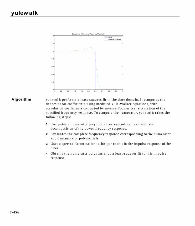
yulewalk
7-456
Algorithm yulewalk performs a least-squares fit in the time domain. It computes thedenominator coefficients using modified Yule-Walker equations, withcorrelation coefficients computed by inverse Fourier transformation of thespecified frequency response. To compute the numerator, yulewalk takes thefollowing steps:
1 Computes a numerator polynomial corresponding to an additivedecomposition of the power frequency response.
2 Evaluates the complete frequency response corresponding to the numeratorand denominator polynomials.
3 Uses a spectral factorization technique to obtain the impulse response of thefilter.
4 Obtains the numerator polynomial by a least-squares fit to this impulseresponse.
0 0.1 0.2 0.3 0.4 0.5 0.6 0.7 0.8 0.9 10
0.2
0.4
0.6
0.8
1
1.2
1.4Comparison of Frequency Response Magnitudes
Ideal yulewalk Designed
yulewalk
7-457
See Also
References [1] Friedlander, B., and B. Porat, “The Modified Yule-Walker Method of ARMASpectral Estimation,” IEEE Transactions on Aerospace Electronic Systems,AES-20, No. 2 (March 1984), pp. 158-173.
butter Butterworth analog and digital filter design.
cheby1 Chebyshev type I filter design (passband ripple).
cheby2 Chebyshev type II filter design (stopband ripple).
ellip Elliptic (Cauer) filter design.
fir2 Window-based finite impulse response filter design –arbitrary response.
firls Least square linear-phase FIR filter design.
maxflat Generalized digital Butterworth filter design.
remez Parks-McClellan optimal FIR filter design.
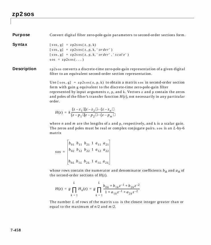
zp2sos
7-458
7zp2sosPurpose Convert digital filter zero-pole-gain parameters to second-order sections form.
Syntax [sos,g] = zp2sos(z,p,k)[sos,g] = zp2sos(z,p,k,'order')[sos,g] = zp2sos(z,p,k,'order','scale')sos = zp2sos(...)
Description zp2sos converts a discrete-time zero-pole-gain representation of a given digitalfilter to an equivalent second-order section representation.
Use [sos,g] = zp2sos(z,p,k) to obtain a matrix sos in second-order sectionform with gain g equivalent to the discrete-time zero-pole-gain filterrepresented by input arguments z, p, and k. Vectors z and p contain the zerosand poles of the filter’s transfer function H(z), not necessarily in any particularorder.
where n and m are the lengths of z and p, respectively, and k is a scalar gain.The zeros and poles must be real or complex conjugate pairs. sos is an L-by-6matrix
whose rows contain the numerator and denominator coefficients bik and aik ofthe second-order sections of H(z).
The number L of rows of the matrix sos is the closest integer greater than orequal to the maximum of n/2 and m/2.
H z( ) kz z1–( ) z z2–( ) z zn–( )z p1–( ) z p2–( ) z pm–( )
--------------------------------------------------------------------=
sos
b01 b11 b21 1 a11 a21
b02 b12 b22 1 a12 a22
b0L b1L b2L 1 a1L a2L
=
H z( ) g Hk z( )
k 1=
L
∏ gb0k b1kz 1– b2kz 2–+ +
1 a1kz 1– a2kz 2–+ +----------------------------------------------------------
k 1=
L
∏= =

zp2sos
7-459
[sos,g] = zp2sos(z,p,k,'order') specifies the order of the rows in sos,where 'order' is:
• 'down', to order the sections so the first row of sos contains the poles closestto the unit circle
• 'up', to order the sections so the first row of sos contains the poles farthestfrom the unit circle (default)
[sos,g] = zp2sos(z,p,k,'order','scale') specifies the desired scaling ofthe gain and the numerator coefficients of all second-order sections, where'scale' is:
• 'none', to apply no scaling (default)
• 'inf', to apply infinity-norm scaling
• 'two', to apply 2-norm scaling
Using infinity-norm scaling in conjunction with up-ordering minimizes theprobability of overflow in the realization. Using 2-norm scaling in conjunctionwith down-ordering minimizes the peak round-off noise.
sos = zp2sos(...) embeds the overall system gain, g, in the first section,H1(z), so that
Example Find a second-order section form of a Butterworth lowpass filter.
[z,p,k] = butter(5,0.2);sos = zp2sos(z,p,k);
H z( ) Hk z( )
k 1=
L
∏=

zp2sos
7-460
Algorithm zp2sos uses a four-step algorithm to determine the second-order sectionrepresentation for an input zero-pole-gain system:
1 It groups the zeros and poles into complex conjugate pairs using thecplxpair function.
2 It forms the second-order section by matching the pole and zero pairsaccording to the following rules:
a Match the poles closest to the unit circle with the zeros closest to thosepoles.
b Match the poles next closest to the unit circle with the zeros closest tothose poles.
c Continue until all of the poles and zeros are matched.
zp2sos groups real poles into sections with the real poles closest to them inabsolute value. The same rule holds for real zeros.
3 It orders the sections according to the proximity of the pole pairs to the unitcircle. zp2sos normally orders the sections with poles closest to the unitcircle last in the cascade. You can tell zp2sos to order the sections in thereverse order by specifying the down flag.
4 zp2sos scales the sections by the norm specified in the 'scale' argument.For arbitrary H(ω), the scaling is defined by
where p can be either ∞ or 2. See the references for details on the scaling.This scaling is an attempt to minimize overflow or peak round-off noise infixed point filter implementations.
H p1
2π------ H ω( ) p ωd
0
2π
1p---
=
zp2sos
7-461
See Also
References [1] Jackson, L.B., Digital Filters and Signal Processing, 3rd ed., KluwerAcademic Publishers, Boston, 1996, Chapter 11.
[2] Mitra, S.K., Digital Signal Processing: A Computer-Based Approach,McGraw-Hill, New York, 1998, Chapter 9.
[3] Vaidyanathan, P.P., “Robust Digital Filter Structures,” Handbook forDigital Signal Processing, S.K. Mitra and J.F. Kaiser, ed., John Wiley & Sons,New York, 1993, Chapter 7.
cplxpair Group complex numbers into complex conjugatepairs.
sos2zp Convert digital filter second-order sectionparameters to zero-pole-gain form.
ss2sos Convert digital filter state-space parameters tosecond-order sections form.
tf2sos Convert digital filter transfer function parameters tosecond-order sections form.
zp2ss Convert zero-pole-gain filter parameters tostate-space form.
zp2tf Convert zero-pole-gain filter parameters to transferfunction form.
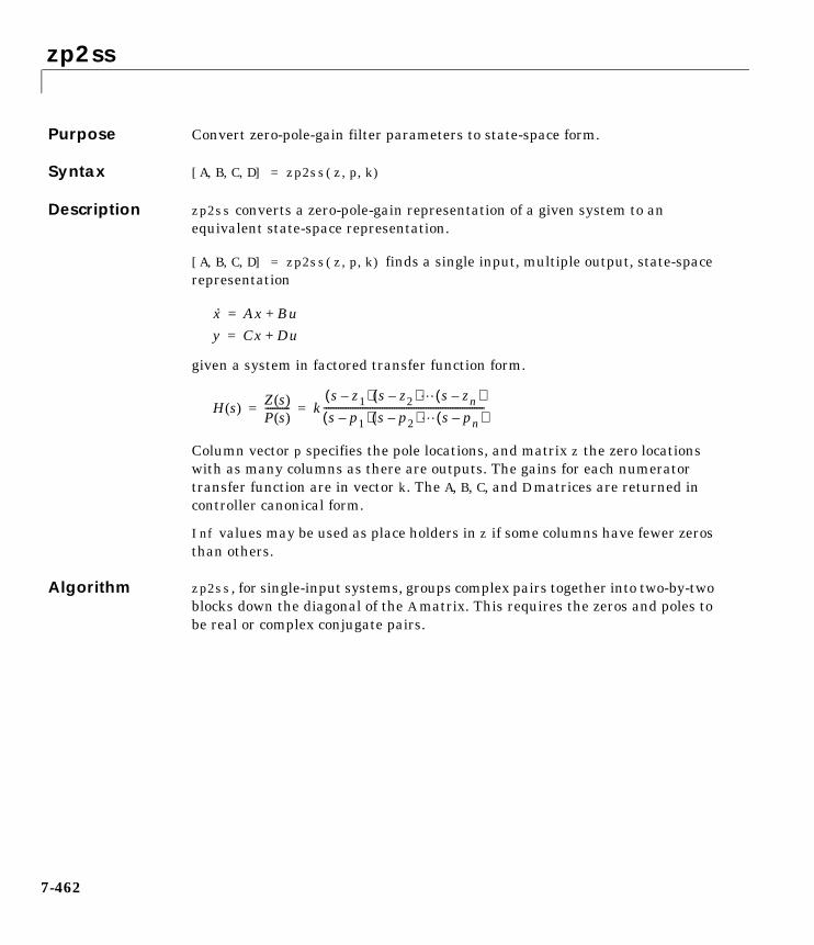
zp2ss
7-462
7zp2ssPurpose Convert zero-pole-gain filter parameters to state-space form.
Syntax [A,B,C,D] = zp2ss(z,p,k)
Description zp2ss converts a zero-pole-gain representation of a given system to anequivalent state-space representation.
[A,B,C,D] = zp2ss(z,p,k) finds a single input, multiple output, state-spacerepresentation
given a system in factored transfer function form.
Column vector p specifies the pole locations, and matrix z the zero locationswith as many columns as there are outputs. The gains for each numeratortransfer function are in vector k. The A, B, C, and D matrices are returned incontroller canonical form.
Inf values may be used as place holders in z if some columns have fewer zerosthan others.
Algorithm zp2ss, for single-input systems, groups complex pairs together into two-by-twoblocks down the diagonal of the A matrix. This requires the zeros and poles tobe real or complex conjugate pairs.
x· Ax Bu+=
y Cx Du+=
H s( )Z s( )P s( )---------- k
s z1–( ) s z2–( ) s zn–( )s p1–( ) s p2–( ) s pn–( )
------------------------------------------------------------------= =
zp2ss
7-463
See Also sos2ss Convert digital filter second-order sectionparameters to state-space form.
ss2zp Convert state-space filter parameters tozero-pole-gain form.
tf2ss Convert transfer function filter parameters tostate-space form.
zp2sos Convert digital filter zero-pole-gain parameters tosecond-order sections form.
zp2tf Convert zero-pole-gain filter parameters to transferfunction form.
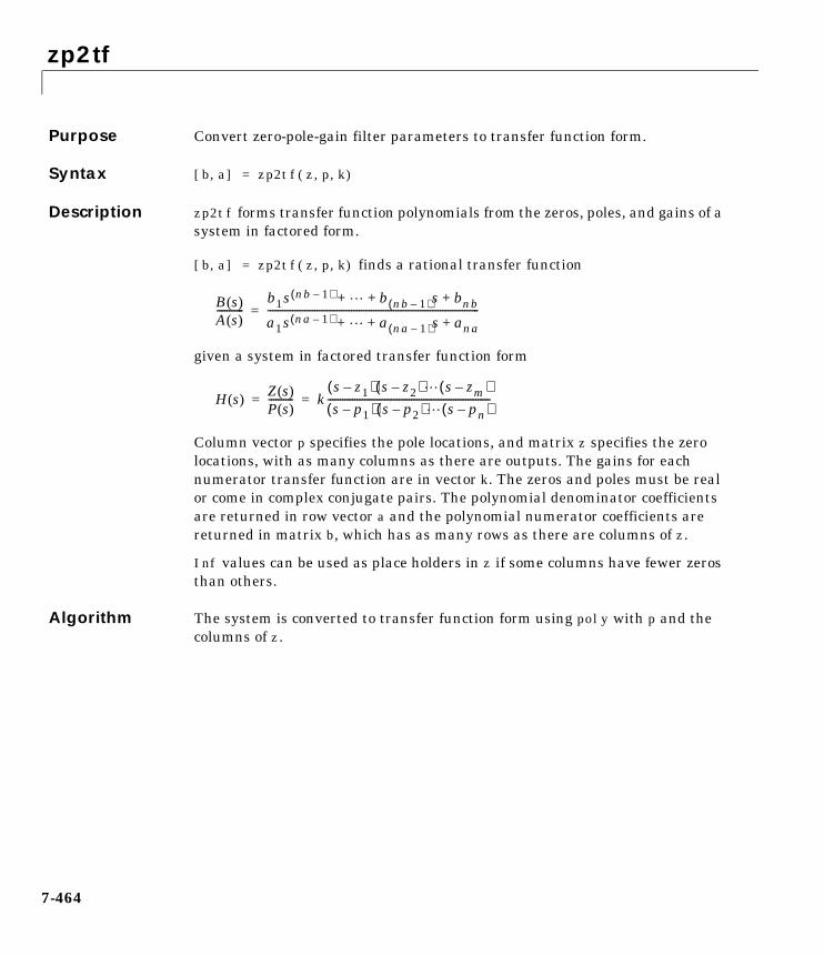
zp2tf
7-464
7zp2tfPurpose Convert zero-pole-gain filter parameters to transfer function form.
Syntax [b,a] = zp2tf(z,p,k)
Description zp2tf forms transfer function polynomials from the zeros, poles, and gains of asystem in factored form.
[b,a] = zp2tf(z,p,k) finds a rational transfer function
given a system in factored transfer function form
Column vector p specifies the pole locations, and matrix z specifies the zerolocations, with as many columns as there are outputs. The gains for eachnumerator transfer function are in vector k. The zeros and poles must be realor come in complex conjugate pairs. The polynomial denominator coefficientsare returned in row vector a and the polynomial numerator coefficients arereturned in matrix b, which has as many rows as there are columns of z.
Inf values can be used as place holders in z if some columns have fewer zerosthan others.
Algorithm The system is converted to transfer function form using poly with p and thecolumns of z.
B s( )A s( )-----------
b1s nb 1–( ) b nb 1–( )s bnb+ + +
a1s na 1–( ) a na 1–( )s ana+ + +--------------------------------------------------------------------------------------=
H s( )Z s( )P s( )---------- k
s z1–( ) s z2–( ) s zm–( )s p1–( ) s p2–( ) s pn–( )
------------------------------------------------------------------= =
zp2tf
7-465
See Also sos2tf Convert digital filter second-order sectionparameters to transfer function form.
ss2tf Convert state-space filter parameters to transferfunction form.
tf2zp Convert transfer function filter parameters tozero-pole-gain form.
zp2sos Convert digital filter zero-pole-gain parameters tosecond-order sections form.
zp2ss Convert zero-pole-gain filter parameters tostate-space form.
zplane
7-466
7zplanePurpose Zero-pole plot.
Syntax zplane(z,p)zplane(b,a)[hz,hp,ht] = zplane(z,p)
Description This function displays the poles and zeros of discrete-time systems.
zplane(z,p) plots the zeros specified in column vector z and the poles specifiedin column vector p in the current figure window. The symbol 'o' represents azero and the symbol 'x' represents a pole. The plot includes the unit circle forreference. If z and p are arrays, zplane plots the poles and zeros in the columnsof z and p in different colors.
You can override the automatic scaling of zplane using
axis([xmin xmax ymin ymax])
or
set(gca,'ylim',[ymin ymax])
or
set(gca,'xlim',[xmin xmax])
after calling zplane. This is useful in the case where one or a few of the zerosor poles have such a large magnitude that the others are grouped tightlyaround the origin and are hard to distinguish.
zplane(b,a) where b and a are row vectors, first uses roots to find the zerosand poles of the transfer function represented by numerator coefficients b anddenominator coefficients a.
[hz,hp,ht] = zplane(z,p) returns vectors of handles to the zero lines, hz,and the pole lines, hp. ht is a vector of handles to the axes/unit circle line andto text objects, which are present when there are multiple zeros or poles. Ifthere are no zeros or no poles, hz or hp is the empty matrix [].
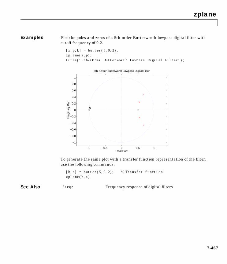
zplane
7-467
Examples Plot the poles and zeros of a 5th-order Butterworth lowpass digital filter withcutoff frequency of 0.2.
[z,p,k] = butter(5,0.2);zplane(z,p);title('5th-Order Butterworth Lowpass Digital Filter');
To generate the same plot with a transfer function representation of the filter,use the following commands.
[b,a] = butter(5,0.2); % Transfer functionzplane(b,a)
See Also
−1 −0.5 0 0.5 1
−1
−0.8
−0.6
−0.4
−0.2
0
0.2
0.4
0.6
0.8
1
5
Real Part
Imag
inar
y P
art
5th−Order Butterworth Lowpass Digital Filter
freqz Frequency response of digital filters.

zplane
7-468

8Filter Design and AnalysisTool Reference

8 Filter Design and Analysis Tool Reference
8-2
Filter Design and Analysis GUI Overview
Choose an analysis method for analyzing your filter design.
Choose the type of filter you want to design.
Choose the filter design method you want to use
Press Design Filter to compute your filter coefficients.
Select the What’s this? button and click on a region of the GUI to access context-sensitive help.
Set quantization parameters for the Filter Design Toolbox.
Set filter specifications. These depend on the type of filter you are designing, as well as the design method you specify.
Specify a filter order or allow it to be estimated.
Zoom in/out.
Use the Filter menu to choose between importing filter coefficients from the MATLAB workspace and designing the filter in the GUI.
Set window specifications for the FIR Window design.
Check this box to quantize the current filter using the Filter Design Toolbox.

Display Region
8-3
Display RegionThe following are displayed in this region:
• The filter specifications. These are initially displayed when you open theGUI.
• The magnitude response plot
• The phase response plot
• The frequency response plots (both magnitude and phase)
• The group delay response plot
• The impulse response plot
• The step response plot
• The pole-zero plot
• The filter coefficients
The plot that is displayed depends on which of the following buttons you’veselected on the toolbar.

8 Filter Design and Analysis Tool Reference
8-4
Display Region: Filter SpecificationsThe Filter Specifications plot is displayed when the Filter Specificationsoption is selected in the Analysis menu, or when the corresponding toolbarbutton is selected.
The plot displays a schematic of the filter parameters (such as Fpass and Fstop)that can be specified in the Design Filter region. The axes use the unitscurrently selected in the Units menus of the Frequency Specifications andMagnitude Specifications regions.
The plot does not reflect the actual values of the filter specifications.
Filter Specifications button

Display Region: Magnitude Response
8-5
Display Region: Magnitude ResponseThe Magnitude Response plot is displayed when the Magnitude Responseoption is selected in the Analysis menu, or when the corresponding toolbarbutton is selected.
The plot shows the actual magnitude response of the current filter. See freqzand freqzplot for more information.
Magnitude Response button

8 Filter Design and Analysis Tool Reference
8-6
Display Region: Phase ResponseThe Phase Response plot is displayed when the Phase Response option isselected in the Analysis menu, or when the corresponding toolbar button isselected.
The plot shows the actual phase response of the current filter. See freqz andfreqzplot for more information.
Phase Response button

Display Region: Magnitude and Phase Response
8-7
Display Region: Magnitude and Phase ResponseThe Magnitude and Phase Response plot is displayed when the Magnitudeand Phase option is selected in the Analysis menu, or when the correspondingtoolbar button is selected.
The plot superposes the magnitude response and the phase response of thecurrent filter. See freqz and freqzplot for more information.
Magnitude and Phase Response button

8 Filter Design and Analysis Tool Reference
8-8
Display Region: Group DelayThe Group Delay plot is displayed when the Group Delay option is selected inthe Analysis menu, or when the corresponding toolbar button is selected.
The plot shows the group delay of the current filter. See grpdelay for moreinformation.
Group Delay button

Display Region: Impulse Response
8-9
Display Region: Impulse ResponseThe Impulse Response plot is displayed when the Impulse Response option isselected in the Analysis menu, or when the corresponding toolbar button isselected.
The plot shows the impulse response of the current filter. See impz for moreinformation.
Impulse Response button

8 Filter Design and Analysis Tool Reference
8-10
Display Region: Step ResponseThe Step Response plot is displayed when the Step Response option is selectedin the Analysis menu, or when the corresponding toolbar button is selected.
The plot shows the step response of the current filter.
Step Response button

Display Region: Pole/Zero Plot
8-11
Display Region: Pole/Zero PlotThe Pole/Zero plot is displayed when the Pole/Zero Plot option is selected inthe Analysis menu, or when the corresponding toolbar button is selected.
The plot shows the pole and zero locations of the current filter on the z-plane.See zplane for more information.
Pole/Zero Plot button

8 Filter Design and Analysis Tool Reference
8-12
Display Region: Filter CoefficientsThe Filter Coefficients viewer is displayed when View Filter Coefficients isselected in the Analysis menu, or when the corresponding toolbar button isselected.
The text box lists the coefficients of the current filter, which depend on thefilter structure (e.g., direct form, lattice, etc.). Use the Convert structurebutton to transform a filter from one structure to another, or use the ImportFilter Coefficients region to directly import a filter with the desired structure.
Filter Coefficients button
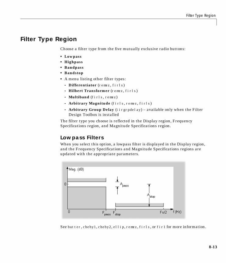
Filter Type Region
8-13
Filter Type RegionChoose a filter type from the five mutually exclusive radio buttons:
• Lowpass• Highpass• Bandpass• Bandstop
• A menu listing other filter types:- Differentiator (remez, firls)- Hilbert Transformer (remez, firls)
- Multiband (firls, remez)
- Arbitrary Magnitude (firls, remez, firls)
- Arbitrary Group Delay (iirgrpdelay) – available only when the FilterDesign Toolbox is installed
The filter type you choose is reflected in the Display region, FrequencySpecifications region, and Magnitude Specifications region.
Lowpass FiltersWhen you select this option, a lowpass filter is displayed in the Display region,and the Frequency Specifications and Magnitude Specifications regions areupdated with the appropriate parameters.
See butter, cheby1, cheby2, ellip, remez, firls, or fir1 for more information.
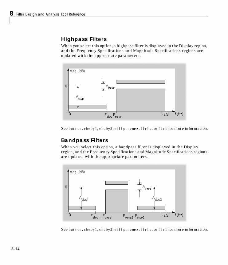
8 Filter Design and Analysis Tool Reference
8-14
Highpass FiltersWhen you select this option, a highpass filter is displayed in the Display region,and the Frequency Specifications and Magnitude Specifications regions areupdated with the appropriate parameters.
See butter, cheby1, cheby2, ellip, remez, firls, or fir1 for more information.
Bandpass FiltersWhen you select this option, a bandpass filter is displayed in the Displayregion, and the Frequency Specifications and Magnitude Specifications regionsare updated with the appropriate parameters.
See butter, cheby1, cheby2, ellip, remez, firls, or fir1 for more information.

Filter Type Region
8-15
Bandstop FiltersYou can specify the frequencies that determine the pass band and thestopband. When you select this option, a bandstop filter is displayed in theDisplay region, and the Frequency Specifications and MagnitudeSpecifications regions are updated with the appropriate parameters.
See butter, cheby1, cheby2, ellip, remez, firls, or fir1 for more information.
Differentiator FiltersA differentiator filter generates the derivative of the input signal. See“Multiband FIR Filter Design with Transition Bands” and remez for moreinformation.
Hilbert Transformer FiltersA Hilbert transformer is a filter that generates an approximation of thediscrete Hilbert transform of the input signal. See “Multiband FIR FilterDesign with Transition Bands” and remez for more information.
Multiband FiltersA multiband filter has multiple passbands interleaved with multiplestopbands. See “Multiband FIR Filter Design with Transition Bands” andremez for more information.

8 Filter Design and Analysis Tool Reference
8-16
Arbitrary Magnitude FiltersAn arbitrary magnitude filter can be designed to have any desired magnituderesponse shape. See “Multiband FIR Filter Design with Transition Bands” andremez for more information.
Arbitrary Group Delay FiltersAn arbitrary group delay filter is an allpass IIR filter which provides the bestapproximation to the specified relative group-delay response in the least-pthsense. This filter type is available only when the Filter Design Toolbox isinstalled. See iirgrpdelay in the Filter Design Toolbox documentation formore information.

Design Method Region
8-17
Design Method RegionThis region allows you to select a filter design method:
• IIR methods
- Butterworth (butter)
- Chebyshev Type I (cheby1)
- Chebyshev Type II (cheby2)
- Elliptic (ellip)- Constrained least Pth-norm- Least Pth-norm
• FIR methods
- Equiripple (remez)
- Least-Squares (firls)
- Window (fir1)
The methods that you see listed depend on the current selection in the FilterType region:
• The Pth-norm designs are only available for the Arbitrary Magnitude andArbitrary Group Delay filter types.
• The Window design is only available for the Lowpass, Highpass,Bandpass, and Bandstop filter type.

8 Filter Design and Analysis Tool Reference
8-18
Current Filter Information Region This region displays important information about the current filter structurebeing used by the tool:
• Filter structure indicates which of the following internal representations isbeing used for the current filter:
- Direct form I- Direct form II- Direct form I transposed- Direct form II transposed- State-space- Lattice allpass- Lattice MA min. phase- Lattice MA max. phase- Lattice ARMA
• Source indicates whether the current filter was designed using FDATool(Designed) or imported from another source (Imported). The term“Quantized” appears here if the filter has been quantized using the FilterDesign Toolbox.
• Order reports the order of the current filter.
• Stable indicates whether the filter is asymptotically stable (Yes) or unstable(No). Filters that have poles on or outside the unit circle are consideredunstable.
• Sections reports the number of sections in the current filter.
The Convert structure button opens a dialog box that allows you to choose adifferent structure for the internal filter representation.

Convert Structure Button
8-19
Convert Structure Button This button opens a dialog box where you can specify a new structure torepresent the current filter. All filters can be converted to the followingrepresentations:
• Direct form I• Direct form II• Direct form I transposed• Direct form II transposed• State-space• Lattice ARMA
In addition, the following conversions are available for particular classes offilters:
• Minimum phase FIR filters can be converted to Lattice MA min. phase
• Maximum phase FIR filters can be converted to Lattice MA max. phase
• Allpass filters can be converted to Lattice allpass
See “Filter Structures” for more information about any of theserepresentations.
When selected, the Use second-order sections check box instructs the tool tostore the converted filter structure as a collection of second-order sectionsrather than as a monolithic higher-order structure. The subordinate Scalemenu lets you select from the following options:
• None (default)• L-2 (L2 norm)• L-infinity (L∞ norm)
The ordering of the second-order sections is optimized for the selected scalingoption. (The tf2sos function that performs the conversion is called with option'down' for L2 norm scaling, and with option 'up' for L∞ norm scaling.)

8 Filter Design and Analysis Tool Reference
8-20
Quantization Region Select Turn quantization on to quantize the current filter using the FilterDesign Toolbox.

Frequency Specifications Region
8-21
Frequency Specifications RegionThe Frequency Specifications region allows you to enter frequency parametersfor the filter design. The options available vary with the selections in the FilterType and Design Method regions:
• Lowpass
- Butterworth
- Chebyshev Type I
- Chebyshev Type II
- Elliptic
- Equiripple
- Least-Squares
- Window
• Highpass
- Butterworth
- Chebyshev Type I
- Chebyshev Type II
- Elliptic
- Equiripple
- Least-Squares
- Window
• Bandpass
- Butterworth
- Chebyshev Type I
- Chebyshev Type II
- Elliptic
- Equiripple
- Least-Squares
- Window
• Bandstop
- Butterworth

8 Filter Design and Analysis Tool Reference
8-22
- Chebyshev Type I
- Chebyshev Type II
- Elliptic
- Equiripple
- Least-Squares
- Window
• Differentiator
• Hilbert Transformer
• Multiband
• Arbitrary Magnitude
• Arbitrary Group Delay – available only when the Filter Design Toolbox isinstalled

Frequency Specifications Region: Lowpass Butterworth
8-23
Frequency Specifications Region: Lowpass ButterworthSelect the units for frequency specifications from the Units list:
• Hz (default)• kHz• MHz• Normalized (0 to 1), where 1 corresponds to the Nyquist frequency
If Specify order is selected in the Filter Order region, specify the followingfrequencies in the text boxes:
• Sampling frequency (Fs) – required when Hz, kHz, or MHz is selected
• Cutoff frequency (Fc or wc) – the frequency at which the magnitude responseis 3 dB below the passband gain
If Minimum order is selected in the Filter Order region, specify the followingfrequencies in the text boxes:
• Sampling frequency (Fs) – required when Hz, kHz, or MHz is selected
• End of the passband (Fpass or wpass)
• Beginning of the stopband (Fstop or wstop)

8 Filter Design and Analysis Tool Reference
8-24
Frequency Specifications Region:Lowpass Chebyshev Type I
Select the units for frequency specifications from the Units list:
• Hz (default)• kHz• MHz• Normalized (0 to 1), where 1 corresponds to the Nyquist frequency
If Specify order is selected in the Filter Order region, specify the followingfrequencies in the text boxes:
• Sampling frequency (Fs) – required when Hz, kHz, or MHz is selected
• End of the passband (Fpass or wpass)
If Minimum order is selected in the Filter Order region, specify the followingfrequencies in the text boxes:
• Sampling frequency (Fs) – required when Hz, kHz, or MHz is selected
• End of the passband (Fpass or wpass)
• Beginning of the stopband (Fstop or wstop)

Frequency Specifications Region: Lowpass Chebyshev Type II
8-25
Frequency Specifications Region:Lowpass Chebyshev Type II
Select the units for frequency specifications from the Units list:
• Hz (default)• kHz• MHz• Normalized (0 to 1), where 1 corresponds to the Nyquist frequency
If Specify order is selected in the Filter Order region, specify the followingfrequencies in the text boxes:
• Sampling frequency (Fs) – required when Hz, kHz, or MHz is selected
• Beginning of the stopband (Fstop or wstop)
If Minimum order is selected in the Filter Order region, specify the followingfrequencies in the text boxes:
• Sampling frequency (Fs) – required when Hz, kHz, or MHz is selected
• End of the passband (Fpass or wpass)
• Beginning of the stopband (Fstop or wstop)

8 Filter Design and Analysis Tool Reference
8-26
Frequency Specifications Region: Lowpass EllipticSelect the units for frequency specifications from the Units list:
• Hz (default)• kHz• MHz• Normalized (0 to 1), where 1 corresponds to the Nyquist frequency
If Specify order is selected in the Filter Order region, specify the followingfrequencies in the text boxes:
• Sampling frequency (Fs) – required when Hz, kHz, or MHz is selected
• End of the passband (Fpass or wpass)
If Minimum order is selected in the Filter Order region, specify the followingfrequencies in the text boxes:
• Sampling frequency (Fs) – required when Hz, kHz, or MHz is selected
• End of the passband (Fpass or wpass)
• Beginning of the stopband (Fstop or wstop)

Frequency Specifications Region: Lowpass Equiripple
8-27
Frequency Specifications Region: Lowpass EquirippleSelect the units for frequency specifications from the Units list:
• Hz (default)• kHz• MHz• Normalized (0 to 1), where 1 corresponds to the Nyquist frequency
If Specify order is selected in the Filter Order region, specify the followingfrequencies in the text boxes:
• Sampling frequency (Fs) – required when Hz, kHz, or MHz is selected
• End of the passband (Fpass or wpass)
• Beginning of the stopband (Fstop or wstop)
If Minimum order is selected in the Filter Order region, specify the followingfrequencies in the text boxes:
• Sampling frequency (Fs) – required when Hz, kHz, or MHz is selected
• End of the passband (Fpass or wpass)
• Beginning of the stopband (Fstop or wstop)

8 Filter Design and Analysis Tool Reference
8-28
Frequency Specifications Region: Lowpass Least-SquaresSelect the units for frequency specifications from the Units list:
• Hz (default)• kHz• MHz• Normalized (0 to 1), where 1 corresponds to the Nyquist frequency
Specify the following frequencies in the text boxes:
• Sampling frequency (Fs) – required when Hz, kHz, or MHz is selected
• End of the passband (Fpass or wpass)
• Beginning of the stopband (Fstop or wstop)

Frequency Specifications Region: Lowpass Window
8-29
Frequency Specifications Region: Lowpass WindowSelect the units for frequency specifications from the Units list:
• Hz (default)• kHz• MHz• Normalized (0 to 1), where 1 corresponds to the Nyquist frequency
If Specify order is selected in the Filter Order region, specify the followingfrequencies in the text boxes:
• Sampling frequency (Fs) – required when Hz, kHz, or MHz is selected
• Cutoff frequency (Fc or wc) – the frequency at which the magnitude responseis 6 dB below the passband gain
If Minimum order is selected in the Filter Order region, specify the followingfrequencies in the text boxes:
• Sampling frequency (Fs) – required when Hz, kHz, or MHz is selected
• End of the passband (Fpass or wpass)
• Beginning of the stopband (Fstop or wstop)

8 Filter Design and Analysis Tool Reference
8-30
Frequency Specifications Region: Highpass ButterworthSelect the units for frequency specifications from the Units list:
• Hz (default)• kHz• MHz• Normalized (0 to 1), where 1 corresponds to the Nyquist frequency
If Specify order is selected in the Filter Order region, specify the followingfrequencies in the text boxes:
• Sampling frequency (Fs) – required when Hz, kHz, or MHz is selected
• Cutoff frequency (Fc or wc) – the frequency at which the magnitude responseis 3 dB below the passband gain
If Minimum order is selected in the Filter Order region, specify the followingfrequencies in the text boxes:
• Sampling frequency (Fs) – required when Hz, kHz, or MHz is selected
• End of the stopband (Fstop or wstop)
• Beginning of the passband (Fpass or wpass)

Frequency Specifications Region: Highpass Chebyshev Type I
8-31
Frequency Specifications Region:Highpass Chebyshev Type I
Select the units for frequency specifications from the Units list:
• Hz (default)• kHz• MHz• Normalized (0 to 1), where 1 corresponds to the Nyquist frequency
If Specify order is selected in the Filter Order region, specify the followingfrequencies in the text boxes:
• Sampling frequency (Fs) – required when Hz, kHz, or MHz is selected
• Beginning of the passband (Fpass or wpass)
If Minimum order is selected in the Filter Order region, specify the followingfrequencies in the text boxes:
• Sampling frequency (Fs) – required when Hz, kHz, or MHz is selected
• End of the stopband (Fstop or wstop)
• Beginning of the passband (Fpass or wpass)

8 Filter Design and Analysis Tool Reference
8-32
Frequency Specifications Region:Highpass Chebyshev Type II
Select the units for frequency specifications from the Units list:
• Hz (default)• kHz• MHz• Normalized (0 to 1), where 1 corresponds to the Nyquist frequency
If Specify order is selected in the Filter Order region, specify the followingfrequencies in the text boxes:
• Sampling frequency (Fs) – required when Hz, kHz, or MHz is selected
• End of the stopband (Fstop or wstop)
If Minimum order is selected in the Filter Order region, specify the followingfrequencies in the text boxes:
• Sampling frequency (Fs) – required when Hz, kHz, or MHz is selected
• End of the stopband (Fstop or wstop)
• Beginning of the passband (Fpass or wpass)

Frequency Specifications Region: Highpass Elliptic
8-33
Frequency Specifications Region: Highpass EllipticSelect the units for frequency specifications from the Units list:
• Hz (default)• kHz• MHz• Normalized (0 to 1), where 1 corresponds to the Nyquist frequency
If Specify order is selected in the Filter Order region, specify the followingfrequencies in the text boxes:
• Sampling frequency (Fs) – required when Hz, kHz, or MHz is selected
• Beginning of the passband (Fpass or wpass)
If Minimum order is selected in the Filter Order region, specify the followingfrequencies in the text boxes:
• Sampling frequency (Fs) – required when Hz, kHz, or MHz is selected
• End of the stopband (Fstop or wstop)
• Beginning of the passband (Fpass or wpass)

8 Filter Design and Analysis Tool Reference
8-34
Frequency Specifications Region: Highpass EquirippleSelect the units for frequency specifications from the Units list:
• Hz (default)• kHz• MHz• Normalized (0 to 1), where 1 corresponds to the Nyquist frequency
If Specify order is selected in the Filter Order region, specify the followingfrequencies in the text boxes:
• Sampling frequency (Fs) – required when Hz, kHz, or MHz is selected
• End of the stopband (Fstop or wstop)
• Beginning of the passband (Fpass or wpass)
If Minimum order is selected in the Filter Order region, specify the followingfrequencies in the text boxes:
• Sampling frequency (Fs) – required when Hz, kHz, or MHz is selected
• End of the stopband (Fstop or wstop)
• Beginning of the passband (Fpass or wpass)

Frequency Specifications Region: Highpass Least-Squares
8-35
Frequency Specifications Region: Highpass Least-SquaresSelect the units for frequency specifications from the Units list:
• Hz (default)• kHz• MHz• Normalized (0 to 1), where 1 corresponds to the Nyquist frequency
Specify the following frequencies in the text boxes:
• Sampling frequency (Fs) – required when Hz, kHz, or MHz is selected
• End of the stopband (Fstop or wstop)
• Beginning of the passband (Fpass or wpass)

8 Filter Design and Analysis Tool Reference
8-36
Frequency Specifications Region: Highpass WindowSelect the units for frequency specifications from the Units list:
• Hz (default)• kHz• MHz• Normalized (0 to 1), where 1 corresponds to the Nyquist frequency
If Specify order is selected in the Filter Order region, specify the followingfrequencies in the text boxes:
• Sampling frequency (Fs) – required when Hz, kHz, or MHz is selected
• Cutoff frequency (Fc or wc) – the frequency at which the magnitude responseis 6 dB below the passband gain
If Minimum order is selected in the Filter Order region, specify the followingfrequencies in the text boxes:
• Sampling frequency (Fs) – required when Hz, kHz, or MHz is selected
• End of the stopband (Fstop or wstop)
• Beginning of the passband (Fpass or wpass)

Frequency Specifications Region: Bandpass Butterworth
8-37
Frequency Specifications Region: Bandpass ButterworthSelect the units for frequency specifications from the Units list:
• Hz (default)• kHz• MHz• Normalized (0 to 1), where 1 corresponds to the Nyquist frequency
If Specify order is selected in the Filter Order region, specify the followingfrequencies in the text boxes:
• Sampling frequency (Fs) – required when Hz, kHz, or MHz is selected
• First cutoff frequency (Fc1or wc1) – the frequency preceding the passbandat which the magnitude response is 3 dB below the passband gain
• Second cutoff frequency (Fc2 or wc2) – the frequency following the passbandat which the magnitude response is 3 dB below the passband gain
If Minimum order is selected in the Filter Order region, specify the followingfrequencies in the text boxes:
• Sampling frequency (Fs) – required when Hz, kHz, or MHz is selected
• End of the first stopband (Fstop1 or wstop1)
• Beginning of the passband (Fpass1 or wpass1)
• End of the passband (Fpass2 or wpass2)
• Beginning of the second stopband (Fstop2 or wstop2)

8 Filter Design and Analysis Tool Reference
8-38
Frequency Specifications Region:Bandpass Chebyshev Type I
Select the units for frequency specifications from the Units list:
• Hz (default)• kHz• MHz• Normalized (0 to 1), where 1 corresponds to the Nyquist frequency
If Specify order is selected in the Filter Order region, specify the followingfrequencies in the text boxes:
• Sampling frequency (Fs) – required when Hz, kHz, or MHz is selected
• Beginning of the passband (Fpass1 or wpass1)
• End of the passband (Fpass2 or wpass2)
If Minimum order is selected in the Filter Order region, specify the followingfrequencies in the text boxes:
• Sampling frequency (Fs) – required when Hz, kHz, or MHz is selected
• End of the first stopband (Fstop1 or wstop1)
• Beginning of the passband (Fpass1 or wpass1)
• End of the passband (Fpass2 or wpass2)
• Beginning of the second stopband (Fstop2 or wstop2)

Frequency Specifications Region: Bandpass Chebyshev Type II
8-39
Frequency Specifications Region:Bandpass Chebyshev Type II
Select the units for frequency specifications from the Units list:
• Hz (default)• kHz• MHz• Normalized (0 to 1), where 1 corresponds to the Nyquist frequency
If Specify order is selected in the Filter Order region, specify the followingfrequencies in the text boxes:
• Sampling frequency (Fs) – required when Hz, kHz, or MHz is selected
• End of the first stopband (Fstop1 or wstop1)
• Beginning of the second stopband (Fstop2 or wstop2)
If Minimum order is selected in the Filter Order region, specify the followingfrequencies in the text boxes:
• Sampling frequency (Fs) – required when Hz, kHz, or MHz is selected
• End of the first stopband (Fstop1 or wstop1)
• Beginning of the passband (Fpass1 or wpass1)
• End of the passband (Fpass2 or wpass2)
• Beginning of the second stopband (Fstop2 or wstop2)

8 Filter Design and Analysis Tool Reference
8-40
Frequency Specifications Region: Bandpass EllipticSelect the units for frequency specifications from the Units list:
• Hz (default)• kHz• MHz• Normalized (0 to 1), where 1 corresponds to the Nyquist frequency
If Specify order is selected in the Filter Order region, specify the followingfrequencies in the text boxes:
• Sampling frequency (Fs) – required when Hz, kHz, or MHz is selected
• Beginning of the passband (Fpass1 or wpass1)
• End of the passband (Fpass2 or wpass2)
If Minimum order is selected in the Filter Order region, specify the followingfrequencies in the text boxes:
• Sampling frequency (Fs) – required when Hz, kHz, or MHz is selected
• End of the first stopband (Fstop1 or wstop1)
• Beginning of the passband (Fpass1 or wpass1)
• End of the passband (Fpass2 or wpass2)
• Beginning of the second stopband (Fstop2 or wstop2)

Frequency Specifications Region: Bandpass Equiripple
8-41
Frequency Specifications Region: Bandpass EquirippleSelect the units for frequency specifications from the Units list:
• Hz (default)• kHz• MHz• Normalized (0 to 1), where 1 corresponds to the Nyquist frequency
If Specify order is selected in the Filter Order region, specify the followingfrequencies in the text boxes:
• Sampling frequency (Fs) – required when Hz, kHz, or MHz is selected
• End of the first stopband (Fstop1 or wstop1)
• Beginning of the passband (Fpass1 or wpass1)
• End of the passband (Fpass2 or wpass2)
• Beginning of the second stopband (Fstop2 or wstop2)
If Minimum order is selected in the Filter Order region, specify the followingfrequencies in the text boxes:
• Sampling frequency (Fs) – required when Hz, kHz, or MHz is selected
• End of the first stopband (Fstop1 or wstop1)
• Beginning of the passband (Fpass1 or wpass1)
• End of the passband (Fpass2 or wpass2)
• Beginning of the second stopband (Fstop2 or wstop2)

8 Filter Design and Analysis Tool Reference
8-42
Frequency Specifications Region: Bandpass Least-SquaresSelect the units for frequency specifications from the Units list:
• Hz (default)• kHz• MHz• Normalized (0 to 1), where 1 corresponds to the Nyquist frequency
Specify the following frequencies in the text boxes:
• Sampling frequency (Fs) – required when Hz, kHz, or MHz is selected
• End of the first stopband (Fstop1 or wstop1)
• Beginning of the passband (Fpass1 or wpass1)
• End of the passband (Fpass2 or wpass2)
• Beginning of the second stopband (Fstop2 or wstop2)

Frequency Specifications Region: Bandpass Window
8-43
Frequency Specifications Region: Bandpass WindowSelect the units for frequency specifications from the Units list:
• Hz (default)• kHz• MHz• Normalized (0 to 1), where 1 corresponds to the Nyquist frequency
If Specify order is selected in the Filter Order region, specify the followingfrequencies in the text boxes:
• Sampling frequency (Fs) – required when Hz, kHz, or MHz is selected
• First cutoff frequency (Fc1or wc1) – the frequency preceding the passbandat which the magnitude response is 6 dB below the passband gain
• Second cutoff frequency (Fc2 or wc2) – the frequency following the passbandat which the magnitude response is 6 dB below the passband gain
If Minimum order is selected in the Filter Order region, specify the followingfrequencies in the text boxes:
• Sampling frequency (Fs) – required when Hz, kHz, or MHz is selected
• End of the first stopband (Fstop1 or wstop1)
• Beginning of the passband (Fpass1 or wpass1)
• End of the passband (Fpass2 or wpass2)
• Beginning of the second stopband (Fstop2 or wstop2)

8 Filter Design and Analysis Tool Reference
8-44
Frequency Specifications Region: Bandstop ButterworthSelect the units for frequency specifications from the Units list:
• Hz (default)• kHz• MHz• Normalized (0 to 1), where 1 corresponds to the Nyquist frequency
If Specify order is selected in the Filter Order region, specify the followingfrequencies in the text boxes:
• Sampling frequency (Fs) – required when Hz, kHz, or MHz is selected
• First cutoff frequency (Fc1or wc1) – the frequency preceding the stopband atwhich the magnitude response is 3 dB below the passband gain
• Second cutoff frequency (Fc2 or wc2) – the frequency following the stopbandat which the magnitude response is 3 dB below the passband gain
If Minimum order is selected in the Filter Order region, specify the followingfrequencies in the text boxes:
• Sampling frequency (Fs) – required when Hz, kHz, or MHz is selected
• End of the first passband (Fpass1 or wpass1)
• Beginning of the stopband (Fstop1 or wstop1)
• End of the stopband (Fstop2 or wstop2)
• Beginning of the second passband (Fpass2 or wpass2)

Frequency Specifications Region: Bandstop Chebyshev Type I
8-45
Frequency Specifications Region:Bandstop Chebyshev Type I
Select the units for frequency specifications from the Units list:
• Hz (default)• kHz• MHz• Normalized (0 to 1), where 1 corresponds to the Nyquist frequency
If Specify order is selected in the Filter Order region, specify the followingfrequencies in the text boxes:
• Sampling frequency (Fs) – required when Hz, kHz, or MHz is selected
• End of the first passband (Fpass1 or wpass1)
• Beginning of the second passband (Fpass2 or wpass2)
If Minimum order is selected in the Filter Order region, specify the followingfrequencies in the text boxes:
• Sampling frequency (Fs) – required when Hz, kHz, or MHz is selected
• End of the first passband (Fpass1 or wpass1)
• Beginning of the stopband (Fstop1 or wstop1)
• End of the stopband (Fstop2 or wstop2)
• Beginning of the second passband (Fpass2 or wpass2)

8 Filter Design and Analysis Tool Reference
8-46
Frequency Specifications Region:Bandstop Chebyshev Type II
Select the units for frequency specifications from the Units list:
• Hz (default)• kHz• MHz• Normalized (0 to 1), where 1 corresponds to the Nyquist frequency
If Specify order is selected in the Filter Order region, specify the followingfrequencies in the text boxes:
• Sampling frequency (Fs) – required when Hz, kHz, or MHz is selected
• Beginning of the stopband (Fstop1 or wstop1)
• End of the stopband (Fstop2 or wstop2)
If Minimum order is selected in the Filter Order region, specify the followingfrequencies in the text boxes:
• Sampling frequency (Fs) – required when Hz, kHz, or MHz is selected
• End of the first passband (Fpass1 or wpass1)
• Beginning of the stopband (Fstop1 or wstop1)
• End of the stopband (Fstop2 or wstop2)
• Beginning of the second passband (Fpass2 or wpass2)

Frequency Specifications Region: Bandstop Elliptic
8-47
Frequency Specifications Region: Bandstop EllipticSelect the units for frequency specifications from the Units list:
• Hz (default)• kHz• MHz• Normalized (0 to 1), where 1 corresponds to the Nyquist frequency
If Specify order is selected in the Filter Order region, specify the followingfrequencies in the text boxes:
• Sampling frequency (Fs) – required when Hz, kHz, or MHz is selected
• End of the first passband (Fpass1 or wpass1)
• Beginning of the second passband (Fpass2 or wpass2)
If Minimum order is selected in the Filter Order region, specify the followingfrequencies in the text boxes:
• Sampling frequency (Fs) – required when Hz, kHz, or MHz is selected
• End of the first passband (Fpass1 or wpass1)
• Beginning of the stopband (Fstop1 or wstop1)
• End of the stopband (Fstop2 or wstop2)
• Beginning of the second passband (Fpass2 or wpass2)

8 Filter Design and Analysis Tool Reference
8-48
Frequency Specifications Region: Bandstop EquirippleSelect the units for frequency specifications from the Units list:
• Hz (default)• kHz• MHz• Normalized (0 to 1), where 1 corresponds to the Nyquist frequency
If Specify order is selected in the Filter Order region, specify the followingfrequencies in the text boxes:
• Sampling frequency (Fs) – required when Hz, kHz, or MHz is selected
• End of the first passband (Fpass1 or wpass1)
• Beginning of the stopband (Fstop1 or wstop1)
• End of the stopband (Fstop2 or wstop2)
• Beginning of the second passband (Fpass2 or wpass2)
If Minimum order is selected in the Filter Order region, specify the followingfrequencies in the text boxes:
• Sampling frequency (Fs) – required when Hz, kHz, or MHz is selected
• End of the first passband (Fpass1 or wpass1)
• Beginning of the stopband (Fstop1 or wstop1)
• End of the stopband (Fstop2 or wstop2)
• Beginning of the second passband (Fpass2 or wpass2)

Frequency Specifications Region: Bandstop Least-Squares
8-49
Frequency Specifications Region: Bandstop Least-SquaresSelect the units for frequency specifications from the Units list:
• Hz (default)• kHz• MHz• Normalized (0 to 1), where 1 corresponds to the Nyquist frequency
Specify the following frequencies in the text boxes:
• Sampling frequency (Fs) – required when Hz, kHz, or MHz is selected
• End of the first passband (Fpass1 or wpass1)
• Beginning of the stopband (Fstop1 or wstop1)
• End of the stopband (Fstop2 or wstop2)
• Beginning of the second passband (Fpass2 or wpass2)

8 Filter Design and Analysis Tool Reference
8-50
Frequency Specifications Region: Bandstop WindowSelect the units for frequency specifications from the Units list:
• Hz (default)• kHz• MHz• Normalized (0 to 1), where 1 corresponds to the Nyquist frequency
If Specify order is selected in the Filter Order region, specify the followingfrequencies in the text boxes:
• Sampling frequency (Fs) – required when Hz, kHz, or MHz is selected
• First cutoff frequency (Fc1or wc1) – the frequency preceding the stopband atwhich the magnitude response is 6 dB below the passband gain
• Second cutoff frequency (Fc2 or wc2) – the frequency following the stopbandat which the magnitude response is 6 dB below the passband gain
If Minimum order is selected in the Filter Order region, specify the followingfrequencies in the text boxes:
• Sampling frequency (Fs) – required when Hz, kHz, or MHz is selected
• End of the first passband (Fpass1 or wpass1)
• Beginning of the stopband (Fstop1 or wstop1)
• End of the stopband (Fstop2 or wstop2)
• Beginning of the second passband (Fpass2 or wpass2)

Magnitude Specifications Region
8-51
Magnitude Specifications RegionThe Magnitude Specifications region allows you to enter magnitudeparameters for the filter design. The options available vary with the selectionsin the Filter Type and Design Method regions:
• Lowpass
- Butterworth
- Chebyshev Type I
- Chebyshev Type II
- Elliptic
- Equiripple
- Least-Squares
- Window
• Highpass
- Butterworth
- Chebyshev Type I
- Chebyshev Type II
- Elliptic
- Equiripple
- Least-Squares
- Window
• Bandpass
- Butterworth
- Chebyshev Type I
- Chebyshev Type II
- Elliptic
- Equiripple
- Least-Squares
- Window
• Bandstop
- Butterworth

8 Filter Design and Analysis Tool Reference
8-52
- Chebyshev Type I
- Chebyshev Type II
- Elliptic
- Equiripple
- Least-Squares
- Window
• Differentiator
• Hilbert Transformer
• Multiband
• Arbitrary Magnitude
• Arbitrary Group Delay – available only when the Filter Design Toolbox isinstalled

Magnitude Specifications Region: Lowpass Butterworth
8-53
Magnitude Specifications Region: Lowpass ButterworthIf Specify order is selected in the Filter Order region, the attenuation at thecutoff frequency is fixed at 3 dB (half the passband power).
If Minimum order is selected in the Filter Order region, select the units formagnitude response characteristics from the Units list:
• dB for magnitude response characteristics in decibels (default)• Squared for squared magnitude response characteristics
Specify the following magnitude response characteristics in the text boxes:
• Passband ripple (Apass or Epass)
• Stopband attenuation (Astop or Estop)

8 Filter Design and Analysis Tool Reference
8-54
Magnitude Specifications Region:Lowpass Chebyshev Type I
If Specify order is selected in the Filter Order region, specify the passbandripple (Apass or Epass) in decibels.
If Minimum order is selected in the Filter Order region, select the units formagnitude response characteristics from the Units list:
• dB for magnitude response characteristics in decibels (default)• Squared for squared magnitude response characteristics
Specify the following magnitude response characteristics in the text boxes:
• Passband ripple (Apass or Epass)
• Stopband attenuation (Astop or Estop)

Magnitude Specifications Region: Lowpass Chebyshev Type II
8-55
Magnitude Specifications Region:Lowpass Chebyshev Type II
If Specify order is selected in the Filter Order region, specify the stopbandattenuation (Astop or Estop) in decibels.
If Minimum order is selected in the Filter Order region, select the units formagnitude response characteristics from the Units list:
• dB for magnitude response characteristics in decibels (default)• Squared for squared magnitude response characteristics
Specify the following magnitude response characteristics in the text boxes:
• Passband ripple (Apass or Epass)
• Stopband attenuation (Astop or Estop)

8 Filter Design and Analysis Tool Reference
8-56
Magnitude Specifications Region: Lowpass EllipticIf Specify order is selected in the Filter Order region, specify the followingmagnitude response characteristics (in dB) in the text boxes:
• Passband ripple (Apass or Epass)
• Stopband attenuation (Astop or Estop)
If Minimum order is selected in the Filter Order region, select the units formagnitude response characteristics from the Units list:
• dB for magnitude response characteristics in decibels (default)• Squared for squared magnitude response characteristics
Specify the following magnitude response characteristics in the text boxes:
• Passband ripple (Apass or Epass)
• Stopband attenuation (Astop or Estop)

Magnitude Specifications Region: Lowpass Equiripple
8-57
Magnitude Specifications Region: Lowpass EquirippleIf Specify order is selected in the Filter Order region, specify the followingrelative weights in the text boxes:
• Passband weighting (Wpass)
• Stopband weighting (Wstop)
If Minimum order is selected in the Filter Order region, select the units formagnitude response characteristics from the Units list:
• dB for magnitude response characteristics in decibels (default)• Linear for linearly scaled magnitude response characteristics
Specify the following magnitude response characteristics in the text boxes:
• Passband ripple (Apass or Dpass)
• Stopband attenuation (Astop or Dstop)

8 Filter Design and Analysis Tool Reference
8-58
Magnitude Specifications Region: Lowpass Least-SquaresSpecify the following relative weights in the text boxes:
• Passband weighting (Wpass)
• Stopband weighting (Wstop)

Magnitude Specifications Region: Lowpass Window
8-59
Magnitude Specifications Region: Lowpass WindowIf Specify order is selected in the Filter Order region, the attenuation at thecutoff frequency is fixed at 6 dB (half the passband gain).
For the Kaiser window option, if Minimum order is selected in the Filter Orderregion, select the units for magnitude response characteristics from the Unitslist:
• dB for magnitude response characteristics in decibels (default)• Linear for linearly scaled magnitude response characteristics
Specify the following magnitude response characteristics in the text boxes:
• Passband ripple (Apass or Dpass)
• Stopband attenuation (Astop or Dstop)

8 Filter Design and Analysis Tool Reference
8-60
Magnitude Specifications Region: Highpass ButterworthIf Specify order is selected in the Filter Order region, the attenuation at thecutoff frequency is fixed at 3 dB (half the passband power).
If Minimum order is selected in the Filter Order region, select the units formagnitude response characteristics from the Units list:
• dB for magnitude response characteristics in decibels (default)• Squared for squared magnitude response characteristics
Specify the following magnitude response characteristics in the text boxes:
• Passband ripple (Apass or Epass)
• Stopband attenuation (Astop or Estop)

Magnitude Specifications Region: Highpass Chebyshev Type I
8-61
Magnitude Specifications Region:Highpass Chebyshev Type I
If Specify order is selected in the Filter Order region, specify the passbandripple (Apass) in decibels.
If Minimum order is selected in the Filter Order region, select the units formagnitude response characteristics from the Units list:
• dB for magnitude response characteristics in decibels (default)• Squared for squared magnitude response characteristics
Specify the following magnitude response characteristics in the text boxes:
• Passband ripple (Apass or Epass)
• Stopband attenuation (Astop or Estop)

8 Filter Design and Analysis Tool Reference
8-62
Magnitude Specifications Region:Highpass Chebyshev Type II
If Specify order is selected in the Filter Order region, specify the stopbandattenuation (Astop) in decibels.
If Minimum order is selected in the Filter Order region, select the units formagnitude response characteristics from the Units list:
• dB for magnitude response characteristics in decibels (default)• Squared for squared magnitude response characteristics
Specify the following magnitude response characteristics in the text boxes:
• Passband ripple (Apass or Epass)
• Stopband attenuation (Astop or Estop)

Magnitude Specifications Region: Highpass Elliptic
8-63
Magnitude Specifications Region: Highpass EllipticIf Specify order is selected in the Filter Order region, specify the followingmagnitude response characteristics (in dB) in the text boxes:
• Passband ripple (Apass or Epass)
• Stopband attenuation (Astop or Estop)
If Minimum order is selected in the Filter Order region, select the units formagnitude response characteristics from the Units list:
• dB for magnitude response characteristics in decibels (default)• Squared for squared magnitude response characteristics
Specify the following magnitude response characteristics in the text boxes:
• Passband ripple (Apass or Epass)
• Stopband attenuation (Astop or Estop)

8 Filter Design and Analysis Tool Reference
8-64
Magnitude Specifications Region: Highpass EquirippleIf Specify order is selected in the Filter Order region, specify the followingrelative weights in the text boxes:
• Stopband weighting (Wstop)
• Passband weighting (Wpass)
If Minimum order is selected in the Filter Order region, select the units formagnitude response characteristics from the Units list:
• dB for magnitude response characteristics in decibels (default)• Linear for linearly scaled magnitude response characteristics
Specify the following magnitude response characteristics in the text boxes:
• Passband ripple (Apass or Dpass)
• Stopband attenuation (Astop or Dstop)

Magnitude Specifications Region: Highpass Least-Squares
8-65
Magnitude Specifications Region: Highpass Least-SquaresSpecify the following relative weights in the text boxes:
• Stopband weighting (Wstop)
• Passband weighting (Wpass)

8 Filter Design and Analysis Tool Reference
8-66
Magnitude Specifications Region: Highpass WindowIf Specify order is selected in the Filter Order region, the attenuation at thecutoff frequency is fixed at 6 dB (half the passband gain).
If Minimum order is selected in the Filter Order region, select the units formagnitude response characteristics from the Units list:
• dB for magnitude response characteristics in decibels (default)• Linear for linearly scaled magnitude response characteristics
Specify the following magnitude response characteristics in the text boxes:
• Passband ripple (Apass or Dpass)
• Stopband attenuation (Astop or Dstop)

Magnitude Specifications Region: Bandpass Butterworth
8-67
Magnitude Specifications Region: Bandpass ButterworthIf Specify order is selected in the Filter Order region, the attenuation at thecutoff frequencies is fixed at 3 dB (half the passband power).
If Minimum order is selected in the Filter Order region, select the units formagnitude response characteristics from the Units list:
• dB for magnitude response characteristics in decibels (default)• Squared for squared magnitude response characteristics
Specify the following magnitude response characteristics in the text boxes:
• Attenuation in the first stopband (Astop1or Estop1)
• Passband ripple (Apass or Epass)
• Attenuation in the second stopband (Astop2 or Estop2)

8 Filter Design and Analysis Tool Reference
8-68
Magnitude Specifications Region:Bandpass Chebyshev Type I
If Specify order is selected in the Filter Order region, specify the passbandripple (Apass) in decibels.
If Minimum order is selected in the Filter Order region, select the units formagnitude response characteristics from the Units list:
• dB for magnitude response characteristics in decibels (default)• Squared for squared magnitude response characteristics
Specify the following magnitude response characteristics in the text boxes:
• Attenuation in the first stopband (Astop1or Estop1)
• Passband ripple (Apass or Epass)
• Attenuation in the second stopband (Astop2 or Estop2)

Magnitude Specifications Region: Bandpass Chebyshev Type II
8-69
Magnitude Specifications Region:Bandpass Chebyshev Type II
If Specify order is selected in the Filter Order region, specify the stopbandattenuation (Astop) in decibels.
If Minimum order is selected in the Filter Order region, select the units formagnitude response characteristics from the Units list:
• dB for magnitude response characteristics in decibels (default)• Squared for squared magnitude response characteristics
Specify the following magnitude response characteristics in the text boxes:
• Attenuation in the first stopband (Astop1or Estop1)
• Passband ripple (Apass or Epass)
• Attenuation in the second stopband (Astop2 or Estop2)

8 Filter Design and Analysis Tool Reference
8-70
Magnitude Specifications Region: Bandpass EllipticIf Specify order is selected in the Filter Order region, specify the followingmagnitude response characteristics (in dB) in the text boxes:
• Stopband attenuation (Astop)
• Passband ripple (Apass)
If Minimum order is selected in the Filter Order region, select the units formagnitude response characteristics from the Units list:
• dB for magnitude response characteristics in decibels (default)• Squared for squared magnitude response characteristics
Specify the following magnitude response characteristics in the text boxes:
• Attenuation in the first stopband (Astop1or Estop1)
• Passband ripple (Apass or Epass)
• Attenuation in the second stopband (Astop2 or Estop2)

Magnitude Specifications Region: Bandpass Equiripple
8-71
Magnitude Specifications Region: Bandpass EquirippleIf Specify order is selected in the Filter Order region, specify the followingrelative weights in the text boxes:
• Weighting in the first stopband (Wstop1)
• Passband weighting (Wpass)
• Weighting in the second stopband (Wstop2)
If Minimum order is selected in the Filter Order region, select the units formagnitude response characteristics from the Units list:
• dB for magnitude response characteristics in decibels (default)• Linear for linearly scaled magnitude response characteristics
Specify the following magnitude response characteristics in the text boxes:
• Attenuation in the first stopband (Astop1 or Dstop1)
• Passband ripple (Apass or Dpass)
• Attenuation in the second stopband (Astop2 or Dstop2)

8 Filter Design and Analysis Tool Reference
8-72
Magnitude Specifications Region: Bandpass Least-SquaresSpecify the following relative weights in the text boxes:
• Weighting in the first stopband (Wstop1)
• Passband weighting (Wpass)
• Weighting in the second stopband (Wstop2)

Magnitude Specifications Region: Bandpass Window
8-73
Magnitude Specifications Region: Bandpass WindowIf Specify order is selected in the Filter Order region, the attenuation at thecutoff frequencies is fixed at 6 dB (half the passband gain).
If Minimum order is selected in the Filter Order region, select the units formagnitude response characteristics from the Units list:
• dB for magnitude response characteristics in decibels (default)• Linear for linearly scaled magnitude response characteristics
Specify the following magnitude response characteristics in the text boxes:
• Attenuation in the first stopband (Astop1 or Dstop1)
• Passband ripple (Apass or Dpass)
• Attenuation in the second stopband (Astop2 or Dstop2)

8 Filter Design and Analysis Tool Reference
8-74
Magnitude Specifications Region: Bandstop ButterworthIf Specify order is selected in the Filter Order region, the attenuation at thecutoff frequencies is fixed at 3 dB (half the passband power).
If Minimum order is selected in the Filter Order region, select the units formagnitude response characteristics from the Units list:
• dB for magnitude response characteristics in decibels (default)• Squared for squared magnitude response characteristics
Specify the following magnitude response characteristics in the text boxes:
• Ripple in the first passband (Apass1 or Epass1)
• Stopband attenuation (Astop or Estop)
• Ripple in the second passband (Apass2 or Epass2)

Magnitude Specifications Region: Bandstop Chebyshev Type I
8-75
Magnitude Specifications Region:Bandstop Chebyshev Type I
If Specify order is selected in the Filter Order region, specify the passbandripple (Apass) in decibels.
If Minimum order is selected in the Filter Order region, select the units formagnitude response characteristics from the Units list:
• dB for magnitude response characteristics in decibels (default)• Squared for squared magnitude response characteristics
Specify the following magnitude response characteristics in the text boxes:
• Ripple in the first passband (Apass1 or Epass1)
• Stopband attenuation (Astop or Estop)
• Ripple in the second passband (Apass2 or Epass2)

8 Filter Design and Analysis Tool Reference
8-76
Magnitude Specifications Region:Bandstop Chebyshev Type II
If Specify order is selected in the Filter Order region, specify the stopbandattenuation (Astop) in decibels.
If Minimum order is selected in the Filter Order region, select the units formagnitude response characteristics from the Units list:
• dB for magnitude response characteristics in decibels (default)• Squared for squared magnitude response characteristics
Specify the following magnitude response characteristics in the text boxes:
• Ripple in the first passband (Apass1 or Epass1)
• Stopband attenuation (Astop or Estop)
• Ripple in the second passband (Apass2 or Epass2)

Magnitude Specifications Region: Bandstop Elliptic
8-77
Magnitude Specifications Region: Bandstop EllipticIf Specify order is selected in the Filter Order region, specify the followingmagnitude response characteristics (in dB) in the text boxes:
• Passband ripple (Apass or Epass)
• Stopband attenuation (Astop or Estop)
If Minimum order is selected in the Filter Order region, select the units formagnitude response characteristics from the Units list:
• dB for magnitude response characteristics in decibels (default)• Squared for squared magnitude response characteristics
Specify the following magnitude response characteristics in the text boxes:
• Ripple in the first passband (Apass1 or Epass1)
• Stopband attenuation (Astop or Estop)
• Ripple in the second passband (Apass2 or Epass2)

8 Filter Design and Analysis Tool Reference
8-78
Magnitude Specifications Region: Bandstop EquirippleIf Specify order is selected in the Filter Order region, specify the followingrelative weights in the text boxes:
• Weighting in the first passband (Wpass1)
• Stopband weighting (Wstop)
• Weighting in the second passband (Wpass2)
If Minimum order is selected in the Filter Order region, select the units formagnitude response characteristics from the Units list:
• dB for magnitude response characteristics in decibels (default)• Linear for linearly scaled magnitude response characteristics
Specify the following magnitude response characteristics in the text boxes:
• Ripple in the first passband (Apass1 or Dpass1)
• Stopband attenuation (Astop or Dstop)
• Ripple in the second passband (Apass2 or Dpass2)

Magnitude Specifications Region: Bandstop Least-Squares
8-79
Magnitude Specifications Region: Bandstop Least-SquaresSpecify the following relative weights in the text boxes:
• Weighting in the first passband (Wpass1)
• Stopband weighting (Wstop)
• Weighting in the second passband (Wpass2)

8 Filter Design and Analysis Tool Reference
8-80
Magnitude Specifications Region: Bandstop WindowIf Specify order is selected in the Filter Order region, the attenuation at thecutoff frequencies is fixed at 6 dB (half the passband gain).
If Minimum order is selected in the Filter Order region, select the units formagnitude response characteristics from the Units list:
• dB for magnitude response characteristics in decibels (default)• Linear for linearly scaled magnitude response characteristics
Specify the following magnitude response characteristics in the text boxes:
• Ripple in the first passband (Apass1 or Dpass1)
• Stopband attenuation (Astop or Dstop)
• Ripple in the second passband (Apass2 or Dpass2)

Frequency and Magnitude Specifications Region: Differentiator
8-81
Frequency and Magnitude Specifications Region:Differentiator
Select the units for frequency specifications from the Frequency units list:
• Hz
• kHz• MHz
• Normalized (0 to 1), where 1 corresponds to the Nyquist frequency
For all units except Normalized, specify the sampling frequency, Fs.
Specify the following parameters in the text boxes:
• Freq. vector – A vector defining the frequency points at which the responsemagnitude is specified, in ascending order. Must have an even length thesame as Mag. vector.
• Mag. vector – A vector defining the response magnitudes at the specifiedfrequencies. Must have an even length the same as Freq. vector.
• Weight vector – A vector defining the relative weight that should be givento each frequency band. Must be half the length of Freq. vector.
Each odd-indexed frequency-amplitude pair defines the left endpoint of a linesegment representing the desired magnitude response in that frequency band.The corresponding even-indexed frequency-amplitude pair defines the rightendpoint. Between the frequency bands specified by these end-points, theremay be undefined sections of the specified frequency response. These are called“don’t care” or “transition” regions, and the magnitude response in these areasis a by-product of the optimization in the other (specified) frequency ranges.
The Weight vector specifies the emphasis to be placed on minimizing the errorin certain frequency bands relative to others, one weight per band. In mostcases, differentiators have only a single band, so the weight is a scalar valuethat does not affect the final filter.
See “Multiband FIR Filter Design with Transition Bands” and remez for moreinformation.

8 Filter Design and Analysis Tool Reference
8-82
Frequency and Magnitude Specifications Region:Hilbert Transformer
Select the units for frequency specifications from the Frequency units list:
• Hz
• kHz• MHz
• Normalized (0 to 1), where 1 corresponds to the Nyquist frequency
For all units except Normalized, specify the sampling frequency, Fs.
Specify the following parameters in the text boxes:
• Freq. vector – A vector defining the frequency points at which the responsemagnitude is specified, in ascending order. Must have an even length thesame as Mag. vector.
• Mag. vector – A vector defining the response magnitudes at the specifiedfrequencies. Must have an even length the same as Freq. vector.
• Weight vector – A vector defining the relative weight that should be givento each frequency band. Must be half the length of Freq. vector.
Each odd-indexed frequency-amplitude pair defines the left endpoint of a linesegment representing the desired magnitude response in that frequency band.The corresponding even-indexed frequency-amplitude pair defines the rightendpoint. Between the frequency bands specified by these end-points, theremay be undefined sections of the specified frequency response. These are called“don’t care” or “transition” regions, and the magnitude response in these areasis a by-product of the optimization in the other (specified) frequency ranges.
The Weight vector specifies the emphasis to be placed on minimizing the errorin certain frequency bands relative to others, one weight per band. In mostcases, Hilbert transformers have only a single band, so the weight is a scalarvalue that does not affect the final filter. However, the Weight vector is usefulwhen designing an antisymmetric multiband filter, such as a Hilberttransformer with stopbands.
See “Multiband FIR Filter Design with Transition Bands” and remez for moreinformation.

Frequency and Magnitude Specifications Region: Multiband
8-83
Frequency and Magnitude Specifications Region:Multiband
Select the units for frequency specifications from the Frequency units list:
• Hz
• kHz• MHz
• Normalized (0 to 1), where 1 corresponds to the Nyquist frequency
For all units except Normalized, specify the sampling frequency, Fs.
Specify the following parameters in the text boxes:
• Freq. vector – A vector defining the frequency points at which the responsemagnitude is specified, in ascending order. Must have an even length thesame as Mag. vector.
• Mag. vector – A vector defining the response magnitudes at the specifiedfrequencies. Must have an even length the same as Freq. vector.
• Weight vector – A vector defining the relative weight that should be givento each frequency band. Must be half the length of Freq. vector.
Each frequency-magnitude pair specifies the junction of two adjacentfrequency bands. See “Multiband FIR Filter Design with Transition Bands”and remez for more information.

8 Filter Design and Analysis Tool Reference
8-84
Frequency and Magnitude Specifications Region:Arbitrary Magnitude
Select the units for frequency specifications from the Frequency units list:
• Hz
• kHz• MHz
• Normalized (0 to 1), where 1 corresponds to the Nyquist frequency
For all units except Normalized, specify the sampling frequency, Fs.
Specify the following parameters in the text boxes:
• Freq. vector – A vector defining the frequency points at which the responsemagnitude is specified, in ascending order. Must have an even length thesame as Mag. vector.
• Mag. vector – A vector defining the response magnitudes at the specifiedfrequencies. Must have an even length the same as Freq. vector.
• Weight vector – A vector defining the relative weight that should be givento each frequency band. Must be half the length of Freq. vector.
Each frequency-magnitude pair specifies the junction of two adjacentfrequency bands. See remez for more information.

Frequency and Magnitude Specifications Region: Arbitrary Group Delay
8-85
Frequency and Magnitude Specifications Region:Arbitrary Group Delay
Select the units for frequency specifications from the Frequency units list:
• Hz
• kHz• MHz
• Normalized (0 to 1), where 1 corresponds to the Nyquist frequency
For all units except Normalized, specify the sampling frequency, Fs.
Specify the following parameters in the text boxes:
• Freq. vector – A vector defining the frequency points at which the responsegroup delay is specified, in ascending order. Must have the same length asGrp. Delay vector.
• Freq. edges – A vector defining the band-edge frequencies on the boundarybetween “care” and “don’t care” regions, in ascending order. The Freq. edgesvector contains a subset of the points in the Freq. vector vector.
• Grp. Delay vector – A vector defining the response group delay in samplesat the specified frequencies. Must have the same length as Freq. vector.
• Weight vector – A vector defining the relative weight that should be givento each frequency-group delay pair. Must have the same length asFreq. vector.
• Max pole radius – A scalar in the range [0 1] specifying the maximumallowable magnitude for any pole.
The Arbitrary Group Delay filter type is available only when the FilterDesign Toolbox is installed. See iirgrpdelay in the Filter Design Toolboxdocumentation for more information.

8 Filter Design and Analysis Tool Reference
8-86
Filter Order RegionSelect a radio button to compute one of the following:
• Filter of the order you specify (Specify order)
• Minimum order filter (Minimum order). The computed filter has theminimum order estimated to meet the specifications.
For certain menu choices in the Design Method region, only one of the aboveorder options is available.
For arbitrary magnitude IIR filters (Filter Type set to Arbitrary Magnitudeand Design Method set to IIR), independently specify the following:
• Order of the transfer function numerator (Numerator order)
• Order of the transfer function denominator (Denominator order)

Window Specification Region
8-87
Window Specification RegionThis region allows you to specify the window type to be used when Window isselected from the FIR menu in the Design Method region. The options are:
• Chebyshev (chebwin)
• Bartlett (bartlett)
• Blackman (blackman)
• Boxcar (boxcar)
• Hamming (hamming)
• Hann (hann)
• Kaiser (kaiser)
• Triangular (triang)
When Chebyshev or Kaiser are selected, the secondary Parameter fieldallows you to specify the Chebyshev stopband ripple magnitude (in dB) or theKaiser β parameter, respectively. See chebwin and kaiser for moreinformation.

8 Filter Design and Analysis Tool Reference
8-88
Import Filter TabSelect the Import Filter tab (or press Ctrl+I) to import filter coefficients fromthe MATLAB workspace, or to enter the filter coefficients directly.
Import Filter Coefficients Region
8-89
Import Filter Coefficients RegionThis region allows you to import a filter by specifying the filter coefficients,either by entering them explicitly, or by referring to variables in the MATLABworkspace. (Access this region by selecting Import Filter from the Filtermenu.)
Select the desired filter representation from the Filter Structure menu:
• Direct form I
• Direct form II
• Direct form I transposed
• Direct form II transposed
• Direct form II (Second-order sections)
• State-space
• Lattice allpass
• Lattice MA min. phase
• Lattice MA max. phase
• Lattice ARMA
• Quantized filter (Qfilt object) — available only when Filter Design Toolboxis installed
The structure that you choose determines the type of coefficients that you needto specify in the text fields to the right. Follow the links above to learn moreabout specifying the coefficients.
Select the frequency units from among the following options in the Units menu:
• Hz (default)
• kHz
• MHz
• Normalized (0 to 1)
For Hz, kHz, and MHz, specify the value of the sampling frequency in the Fsfield.

8 Filter Design and Analysis Tool Reference
8-90
Import Filter Coefficients: Direct FormSpecify the Numerator and Denominator polynomial coefficients using anyvalid MATLAB variable or expression. See “Filter Structures” for moreinformation.
Press Clear to erase the coefficients.

Import Filter Coefficients: Direct Form II (Second-Order Sections)
8-91
Import Filter Coefficients:Direct Form II (Second-Order Sections)
Specify the Gain and SOS Matrix using any valid MATLAB variable orexpression. See “Filter Structures” for more information.
Press Clear to erase the coefficients.

8 Filter Design and Analysis Tool Reference
8-92
Import Filter Coefficients: State-SpaceSpecify the A, B, C, and D matrices using any valid MATLAB variable orexpression. See “Filter Structures” for more information.
Press Clear to erase the matrices.

Import Filter Coefficients: Lattice
8-93
Import Filter Coefficients: LatticeSpecify the Lattice coeff and Ladder coeff coefficients using any validMATLAB variable or expression. See “Filter Structures” for more information.
Press Clear to erase the coefficients.
8 Filter Design and Analysis Tool Reference
8-94
Import Filter Coefficients: Quantized Filter (Qfilt Object)Specify a Qfilt object. See qfilt in the Filter Design Toolbox for moreinformation.
Press Clear to erase the data.

Design Filter Tab
8-95
Design Filter Tab Select the Design Filter tab (or press Ctrl+D) to design a filter by specifyingthe filter requirements.

8 Filter Design and Analysis Tool Reference
8-96
Import Filter ButtonSelect this button to import filter coefficients while in the import mode.

Design Filter Button
8-97
Design Filter ButtonSelect this button to design the filter that you specified in the GUI.

8 Filter Design and Analysis Tool Reference
8-98
I-1
Index
AA/D conversion 7-437abs 7-16ac2poly 7-17ac2rc 7-18aliased sinc functions 1-13
command for 7-128aliasing
impulse invariance 2-42preventing 4-22reducing 4-39
all-pole filters. See IIR filtersall-zero filters. See FIR filtersam 4-30AM. See amplitude modulationamdsb–sc 4-30, 7-264amdsb–tc 4-30, 7-264amplitude demodulation
double side-band, suppressed carrier 7-125double side-band, transmitted carrier 7-125single side-band 7-125
amplitude modulation 4-30double side-band, suppressed carrier 7-264double side-band, transmitted carrier 7-264quadrature 4-31single side-band 7-264
amssb 4-31, 7-264analog filters 2-39
bandpass 7-247bandstop 7-250Bessel 2-12, 2-39, 7-26, 7-27bilinear transformation 2-43Butterworth 2-9, 2-39, 7-48, 7-49, 7-50Chebyshev 2-39Chebyshev type I 2-10, 7-62, 7-75Chebyshev type II 2-11, 7-81converting to digital 2-42, 7-215
design 2-8discretization 2-42elliptic 2-39, 7-136frequency response 1-27, 2-13, 7-185highpass 7-252impulse invariance 2-42inverse 7-226lowpass 7-254order estimation
Butterworth 7-55Chebyshev type I 7-64, 7-69Chebyshev type II 7-69elliptic 7-144
plotting 2-13representational models 1-42See also IIR filters
analog frequency 29analog signals. See signalsanalytic signals 7-207angle 7-19anti-symmetric filters 2-26AR filters, stability check 7-316AR models. See autoregressive (AR) modelsarburg 4-12, 7-20arcov 4-12, 7-21ARMA filters 1-16, 4-14, 4-16
Prony’s method 4-14Steiglitz-McBride method 4-16See also IIR filters
armcov 4-12, 7-22ARX models 4-14aryule 4-12, 7-23ASCII files, importing 1-14autocorrelation 7-314, 7-448autocorrelation sequences
converting from reflection coefficients 7-341
Index
I-2
estimation, variance 3-4filter coefficients
converting to and from 7-17, 7-18, 7-314filters, multiple channels 3-5two-dimensional 7-451
autocovariance 7-452multiple channels 3-5
autoregressive (AR) models 1-16Burg method 7-20, 7-267, 7-271covariance method 7-21, 7-273modified covariance method 7-22, 7-293,
7-297Yule-Walker AR method 7-23, 7-335, 7-339See also IIR filters
autoregressive moving average (ARMA) filters.See ARMA filters
averaging filters 1-15axis labels 6-50axis parameters
Filter Viewer 6-50Spectrum Viewer 6-50
Bband edges, prewarping 2-44bandlimited interpolation 7-382bandpass filters 7-55, 7-64, 7-69, 7-144
Bessel 7-27Butterworth 7-49Chebyshev type I 7-75, 7-77Chebyshev type II 7-80design 2-7elliptic 7-136example, Chebyshev type I 2-40FIR 2-22, 7-167impulse invariance 2-42transformation from lowpass to 7-247
bandstop filters 2-7, 7-55, 7-64, 7-69, 7-144Bessel 7-27Butterworth 7-50Chebyshev type I 7-76Chebyshev type II 7-80elliptic 7-137FIR 2-22, 7-166transformation from lowpass to 7-250
bandwidth 2-41bartlett 4-3, 7-24
example 4-3triang, comparison to 7-24
Bartlett windows 4-3coefficients 7-24
Bessel filters 2-12, 2-39, 7-26bandpass 7-27bandstop 7-27characteristics 2-12highpass 7-27limitations 7-29lowpass 7-27roots 7-26
besselap 2-6, 7-26example 2-12
besself 2-6, 2-7, 7-27bias
correlation 3-4, 4-13power spectral density 3-17, 3-18, 3-23variance trade-off 3-4
bilinear 2-6, 2-42, 2-43, 7-31bilinear transformations 2-43, 2-44, 7-31
output representation 7-32prewarping 2-44, 7-31
blackman 4-3, 7-36Blackman windows 4-5, 7-36boxcar 4-3, 7-38
example 4-3
Index
I-3
boxcar windows. See rectangular windowsbrackets, indicating closed interval 29buffering 7-39Burg method 3-8, 3-9, 3-33
example 3-34Welch’s method, comparison 3-35
buttap 2-6, 7-48example 2-9
butter 2-6, 2-7, 7-49Butterworth filters 2-9, 2-39, 7-48
bandpass 7-49bandstop 7-50characteristics 2-9design 7-49generalized 2-15highpass 7-50limitations 7-53lowpass 7-49order estimation 2-8, 7-54
buttord 2-6, 7-54
Ccanonical forms 1-18, 7-423carrier frequency 4-30, 7-264, 7-445carrier signals 4-30, 7-125cascade, filters 1-38Cauer filters. See elliptic filterscceps 4-24, 4-26, 7-59
example 4-24cell2sos 7-61center frequency 2-41central features 1-2cepstrum
analysis 4-24applications 4-24complex 4-24
inverse 4-24, 4-26overview 4-24real 4-24, 4-25, 7-346reconstructing signals (minimum-phase) 4-26
cheb1ap 2-6, 7-62example 2-10, 2-40
cheb1ord 2-6, 7-63cheb2ap 2-6, 7-67
example 2-11cheb2ord 2-6, 7-68chebwin 4-3, 7-73, 7-98cheby1 2-6, 2-7, 7-75
example 2-45cheby2 2-6, 2-7, 7-80Chebyshev error minimization 2-23, 7-348Chebyshev type I filters 2-10, 2-39, 7-62, 7-75
bandpass 7-75, 7-77bandstop 7-76characteristics 2-10design 7-75highpass 7-76lowpass 7-75order estimation 2-8, 7-63
Chebyshev type II filters 2-39, 7-80bandpass 7-80bandstop 7-80characteristics 2-11highpass 7-80limitations 7-79lowpass 7-80order estimation 2-8
Chebyshev windows 4-9, 7-73frequency response 4-9
chirp 1-10, 7-85chirp signals 1-10chirp z-transforms (CZT) 4-35, 7-116
discrete Fourier transforms, comparison 4-35
Index
I-4
frequency analysis, narrowband 7-116coding, PCM 7-437coefficients
correlation 7-97filter 1-16, 6-38, 7-17, 7-314, 7-316, 7-344linear prediction 7-256reflection 1-38, 7-18, 7-316, 7-341, 7-344sequence 7-341
cohere 3-9, 3-29, 7-88linearly dependent data 3-30
coherence 3-29, 7-88linearly dependent data 3-30
colors, SPTool 6-50communications 4-11, 4-30, 7-264
See also modulation, demodulation, voltagecontrolled oscillation
communications simulation 7-125compact disc standards 4-21compaction 4-38complex conjugate 7-102complex envelope. See Hilbert transformscomplex numbers, grouping by conjugate 7-102confidence intervals
cross spectral density 3-27power spectral density 3-27warnings 3-27
context-sensitive help 5-6, 6-17continuous signals. See signalscontinuous-time filters. See analog filterscontrol systems 1-36Control Systems Toolbox 1-36, 7-219, 7-411conv 1-15, 1-21, 7-92conv2 1-15, 7-93conventions in our documentation (table) 30conversions
autocorrelation sequences to and from filtercoefficients 7-17
autocorrelation sequences to and from reflectioncoefficients 7-18
filter coefficients to autocorrelation sequences7-314
filter coefficients to reflection coefficients 7-316,7-344
functions (table) 1-43reflection coefficients to autocorrelation
sequences 7-341second-order section forms to state-space forms
7-385second-order section forms to transfer functions
7-387second-order section forms to zero-pole-gain
forms 7-389state-space forms to second-order section forms
7-403state-space forms to zero-pole-gain forms 7-409transfer functions to lattice forms 7-417transfer functions to second-order section forms
7-418transfer functions to state-space forms 7-422zero-pole-gain forms to second-order section
forms 7-458zero-pole-gain forms to state-space forms 7-462
convmtx 1-41, 1-43, 7-95convolution 7-92
cross-correlation 3-3example 1-15filtering 1-15, 7-161matrices for 1-41, 1-43, 7-95
example 7-95two-dimensional 7-93
corrcoef 7-97correlation 3-2
bias 3-4, 4-13coefficient matrices 7-97
Index
I-5
cross-correlation 7-447matrices
covariance method 7-98modified covariance method 7-98
See also autocorrelation sequences,cross-correlation sequences
correlation matrices 7-98corrmtx 7-98cosine windows 4-5cov 7-101covariance 3-2
matrices 7-101See also autocovariance, cross-covariance
covariance method 3-9, 3-36, 7-277example 3-36See also modified covariance method
cplxpair 7-102cremez 2-17, 7-103cross spectral density 3-27, 7-111
confidence intervals 3-27See also power spectral density, spectral
estimationcross-correlation sequences 3-3
estimation 7-447biased 3-4unbiased 3-4
filters, multiple channels 3-5normalization 3-5two-dimensional 7-451
cross-covariance 3-3, 7-452multiple channels 3-5
csd 3-9, 3-27, 7-111cutoff frequency 2-39, 7-27czt 4-36, 7-116CZT. See chirp z-transforms
DD.C. component suppression 1-47data
multichannel 1-5, 1-8vectors 1-7
data compression 4-11data matrices 1-5, 1-8data vectors 1-5dct 4-37, 7-119
example 4-38decimate 7-121decimation 7-121
FIR filter for 7-223decoding 7-434deconv 4-34, 7-124
example 4-34deconvolution 4-34, 7-124default session file 6-50delays
group 1-29noninteger 2-27phase 1-29signals 2-27
demod 4-30, 4-31, 7-125example 4-31
demodulation 4-31, 7-125amplitude, quadrature 7-126example 4-31methods 4-31, 7-125phase 7-126pulse time 7-126pulse width 7-126
DFT. See discrete Fourier transformsdftmtx 7-127difference equations 1-33differentiators 2-27, 7-179, 7-350digital audio tape standards 4-21
Index
I-6
digital filtersanti-causal 1-21Butterworth 7-49cascade 1-38Chebyshev type I 7-75Chebyshev type II 7-80coefficients 1-16convolution matrices 1-41design 2-3elliptic 7-136FIR 2-17
IIR, comparison to 2-17fixed-point implementation 1-38frequency data, identification from 7-230frequency response 1-25group delay 1-29, 7-200IIR 2-5
FIR filters, comparison to 2-5implementation 1-15, 7-155, 7-158
convolution 1-15FFT-based (FIR) 7-155filter 1-17overlap-add method 1-23
impulse response 1-15, 1-24, 7-217initial conditions 1-18linear models 1-33models 1-33names 1-16order 1-16
state-space representation 1-35order estimation
Butterworth 7-54, 7-63, 7-68Chebyshev type I 7-63, 7-68Chebyshev type II 7-68elliptic 7-143equiripple FIR 7-356
phase delays 1-29, 7-200
poles 1-31, 1-34second-order sections 1-38specifications 2-8startup transients 1-22structures
lattice/ladder 1-38transposed direct form II 1-18
time-domain representation 1-17transfer functions representation 1-16transients 1-23two-dimensional 7-161zero-phase 1-21, 7-162zeros 1-31, 1-34See also FIR filters, IIR filters
digital frequency 29direct design 2-6diric 7-128Dirichlet functions 1-13
command for 7-128discrete cosine transforms (DCT) 7-119
applications 4-37energy compaction property 4-38example 4-38inverse 4-37, 7-211signals, reconstructing 4-38
discrete Fourier transforms (DFT) 1-3, 1-45, 2-27,7-151
algorithms 1-46applications 7-151eigenvector equivalent 3-38example 1-46IIR filter implementation 1-23inverse 1-45, 7-213
matrices 7-127two-dimensional 1-47, 7-214
magnitude 1-46matrices 7-127
Index
I-7
phase 1-46signal length dependencies 1-46spectral analysis 3-6, 3-10time-dependent 4-28two-dimensional 1-47, 7-154See also fast Fourier transforms (FFT), fft
discrete prolate spheroidal sequencesSee DPSS
discretization 7-215bilinear transformations 2-43
prewarping 2-44impulse invariance 2-42
discretization, filters 2-42disk, loading variables from 6-47division, polynomials 7-124DPSS
direct method 7-130interpolation 7-129
dpss 7-129dpss.mat 3-26dpssclear 3-26, 7-132dpssdir 3-26, 7-133dpssload 3-26, 7-134dpsssave 3-26, 7-135duty cycles 1-9
Eechoes, detection 4-24edge effects 1-23eigenanalysis 3-37
frequency estimation 3-37eigenvector method 3-8, 3-36, 7-279
root MUSIC 7-368See also multiple signal classification method
ellip 2-6, 2-7, 7-136ellipap 2-6, 7-142
example 2-11ellipord 2-6, 7-143, 7-148elliptic filters 2-39, 7-136
bandpass 7-136bandstop 7-137characteristics 2-11highpass 7-137limitations 7-140lowpass 7-136order estimation 2-8, 7-143, 7-148
encodingPCM 7-437uniform 7-437
eqtflength 7-148equiripple characteristics
Chebyshev type I filters (passband) 2-10Chebyshev type II filters (stopband) 2-11Chebyshev windows 4-9elliptic filters 2-11, 7-136, 7-142Parks-McClellan design 7-348
equiripple filters 2-23error minimization
desired and actual response, between 2-23frequency bands, weighting 2-26minimax 2-23
estimationcross spectral density 3-27nonparametric
multiple signal classification method(MUSIC) 3-8
multitaper method (MTM) 3-8Welch’s method 3-8
parametric 3-8Burg method 7-20covariance method 7-21modified covariance method 7-22Yule-Walker method 7-23
Index
I-8
spectral density 3-8, 3-10transfer functions 3-28See also parametric modeling
Ffast Fourier transforms (FFT) 1-23, 1-45
fft 1-23frequency response 1-25radix-2 algorithm 7-153signal processing, role in 1-45two-dimensional 7-154
fdatool 5-1context-sensitive help 5-6help on 5-6, 6-17opening 5-5
fft 1-3, 1-23, 1-45, 7-151example 1-46execution time 1-46number of samples 1-46output 1-47, 7-157radix-2 algorithm 7-153
FFT filtering 1-23FFT. See fast Fourier transformsfft2 1-47, 7-154
output 1-47fftfilt 1-20, 7-155
filter, comparison to 7-155fftshift 1-47, 1-47, 7-157filter
coefficients 1-16median 4-29order 1-16
filter 1-3, 1-17, 1-21, 7-158fftfilt, comparison to 7-155filtfilt, comparison 1-22final condition parameters 1-18
implementation 1-18initial condition parameters 1-18initial conditions 7-163
filter coefficientsreflection coefficients, conversions to 7-316,
7-344filter design graphical user interface. See fdatoolfilter design GUI 5-2
analysis buttons 5-13analysis functions 5-13computing coefficients 5-12context-sensitive help 5-6design methods 5-8design sessions
opening 5-21saving 5-21
exporting filters 5-19filter design specification 5-9filter order specification 5-11filter type 5-7filters
architecture 5-14implementation 5-14realization 5-14structure 5-14
frequency response specification 5-9group delay 5-13help on 5-6importing coefficients 5-16importing filters 5-16impulse response 5-13magnitude response 5-13magnitude response specs 5-10opening 5-5phase delay 5-13phase response 5-13pole-zero plots 5-13

Index
I-9
saving coefficients 5-19step response 5-13
Filter Designer 6-8, 7-397FFT length 6-50filter types 6-8filters
editing 6-45redesigning 6-37saving 6-33
FIR filters 6-8FIR methods 6-8grid lines 6-50IIR methods 6-8opening 6-9, 6-22overview 6-8plots
customizing 6-50magnitude 6-37
Pole/Zero Editor 6-34sample frequency 6-38spectra, overlaying 6-9zooming 6-50
filter parameters 6-50Filter Viewer 6-11, 7-399
axis parameters 6-50filter parameters 6-50measurements 6-51opening 6-11overview 6-11preferences, tiling 6-50printing 6-28rulers 6-51zooming 6-50
filter2 7-161filters 1-3
analog 2-9, 2-12, 7-26, 7-48, 7-62anti-causal 1-21
anti-symmetric 2-26averaging 1-15bandpass
Butterworth 7-54Chebyshev type I 7-63Chebyshev type II 7-68elliptic 7-143
bandstopButterworth 7-54Chebyshev type I 7-63Chebyshev type II 7-68elliptic 7-143
Butterworth 2-8, 7-49generalized 2-15
Chebyshev 2-8type I 7-75type II 7-80
coefficients 1-17, 1-33, 2-18, 6-38converting to autocorrelation sequence
7-314convolution 1-15creating 2-8design 6-8
Filter Designer 6-8FIR 2-23generalized 2-6
discretization 2-42elliptic 2-8, 7-136equiripple 2-23FIR 7-348
single band 2-21frequency data, identification from 7-226frequency domain 1-23frequency transformation functions 2-39, 2-40highpass
Butterworth 7-54Chebyshev type I 7-63
Index
I-10
Chebyshev type II 7-68elliptic 7-143
implementation 1-23, 7-155, 7-158initial conditions 1-18, 1-19inverse 7-226, 7-230lattice/ladder 1-38linear phase 2-17, 2-18linear time-invariant digital 1-3lowpass
Butterworth 7-54Chebyshev type I 7-63Chebyshev type II 7-68elliptic 7-143
measurements 6-51median 7-263minimax 2-23minimum phase 7-319names 1-16order 1-16, 2-8, 7-54, 7-63, 7-143, 7-148order estimation 2-8phase, modulation 4-26prediction 4-13quantized, state vectors 7-159Savitzky-Golay 7-378, 7-380Schur realizations 7-375second-order section forms 1-38, 1-44, 7-391specifications 2-8SPTool 6-43transposed direct form II structure 1-18two-dimensional 7-161types 2-18zero-phase 1-21, 7-162See also FIR filters, IIR filters, digital filters,
analog filtersfiltfilt 1-20, 1-21, 2-5, 7-162
example 1-21filter, comparison 1-22
initial conditions 1-22filtic 1-19, 7-163FIR filters 1-16, 2-17
decimation 7-223differentiators 2-27, 7-179, 7-350equiripple 2-17, 2-23, 2-24example 6-18Filter Designer 6-8frequency domain 1-20frequency response 7-169Hilbert transformers 2-26, 7-179, 7-350IIR filters, comparison 2-17implementation 1-18, 7-158
FFT-based 1-23, 7-155overlap-add method 1-23, 7-155
interpolation 7-223Kaiser windows 4-7lattice/ladder 1-38least squares 2-17, 2-24, 7-178
constrained 2-17, 2-28equiripple, comparison 2-24linear phase 2-29multiband 2-29, 2-30weighted 2-31
linear phase 2-18, 2-23, 7-178, 7-348multiband 2-17, 2-22, 2-23order estimation, remez 7-356overlap-add method 7-155Parks-McClellan method 2-23, 7-348raised cosine method 2-17resampling 1-20responses 2-32
complex filters 2-17, 7-103delays, reducing 2-35nonlinear phase 2-17, 7-103
standard band 2-21types 7-181, 7-353

Index
I-11
windowing method 2-17windows 2-19, 7-165
fir1 2-17, 2-21fir2 2-17, 2-21fircls 2-17, 7-172fircls1 2-17, 7-175firls 2-17, 2-23, 7-178
differentiators 2-27filter characteristics 7-181remez, comparison to 2-24weight vectors 2-26
firrcos 2-17, 7-183fixed-point implementation, digital filters 1-38fm 4-31FM. See frequency modulationfopen 1-14Fourier transforms. See discrete Fourier
transforms, fast Fourier transformsfread 1-14freqs 1-27, 7-185freqspace 7-188frequency 7-349
analog 29angular 2-3carrier 4-30, 7-264, 7-445center 2-41cutoff 2-39digital 29estimation
eigenanalysis 3-37eigenvector (EV) method 3-37multiple signal classification (MUSIC)
method 3-37normalization 2-3Nyquist 29, 2-3prewarping 7-31vectors 2-25, 7-169, 7-172, 7-455
frequency analysis, time-dependent 7-392frequency demodulation 7-126frequency domain
duality with time-domain 1-23filters 1-23FIR filtering 1-20transformation functions 2-39, 7-247, 7-250,
7-252, 7-254example 2-41lowpass to bandpass 7-247lowpass to bandstop 7-250lowpass to highpass 7-252
frequency domain based modeling. See parametricmodeling
frequency modulation 7-265frequency response 1-25, 2-14, 7-169
Bessel filters 2-12Butterworth filters 2-9Chebyshev type I filters 2-10Chebyshev type II filters 2-11Chebyshev windows 4-9elliptic filters 2-11error minimization 2-23evaluating 1-25example 1-26inverse 7-226Kaiser window 4-6linear phase 2-18magnitude 1-27monotonic 2-9multiband 2-14phase 1-27
unwrapping 1-28plotting 1-26, 7-193samples, spacing 7-188sampling frequency 1-25
frequency vectors 7-349
Index
I-12
freqz 1-25, 7-189sampling frequencies 1-25sampling frequency 1-25spacing 7-188
freqzplot 7-193From Disk radio button 6-47fscanf 1-14
Ggains, scalar 1-34gauspuls 1-10, 1-11, 7-196, 7-198, 7-199Gauss-Newton method 7-229, 7-232generalized Butterworth filters 2-15generalized cosine windows 4-5generalized filters 2-6Gibbs effect 2-20
reduced by window 4-3graphical user interface (GUI) 1-4
See also interactive tools, SPToolgrid lines 6-50group delay 1-29, 2-18, 7-200
example 1-30passband 2-12
grpdelay 1-29, 7-200GUI-based tools. See interactive tools
Hhamming 4-3, 7-203Hamming windows 2-20, 3-18, 4-5, 7-203hann 7-205Hann windows 7-205Hanning windows 4-5, 7-205hanning. See hannhighpass filters 2-7, 7-55, 7-64, 7-69, 7-144
Bessel 7-27
Butterworth 7-50Chebyshev type I 7-76Chebyshev type II 7-80elliptic 7-137FIR 2-22, 7-167lowpass, transformation from 7-252
hilbert 2-27, 4-39example 4-39
Hilbert transformers 7-179, 7-350Hilbert transforms 4-35, 4-39, 7-207
analytic signals, of 2-27example 4-39instantaneous attributes 4-40
homomorphic systems 4-24Hz 7-268, 7-274, 7-294, 7-336
Iicceps 4-24, 4-26, 7-210
example 4-27idct 4-37, 7-211ideal lowpass filters 2-19
See also lowpass filtersifft 1-45, 7-213
samples, specifying 1-47ifft2 1-47, 1-47, 7-214IIR filters 2-5, 2-6, 2-8, 2-9, 2-14
Bessel 2-12Butterworth 2-8, 2-9Butterworth, generalized 2-15Chebyshev 2-8, 2-10, 2-11Chebyshev type I 2-10Chebyshev type II 2-11design 2-7, 2-38elliptic 2-8, 2-11Filter Designer 6-8filter types, comparison 2-9
Index
I-13
FIR filters, comparison to 2-5frequency response 2-14implementation 7-158
frequency domain 1-23zero-phase 1-21
lattice/ladder 1-38Levinson-Durbin recursion 7-245maximally flat 2-15multiband 2-14order estimation 2-8plotting responses 2-13Prony’s method 7-320specifications 2-8Steiglitz-McBride iteration 7-412Yule-Walker 2-14, 7-455See also direct design
image processing 1-47, 7-93impinvar 2-6, 2-42, 7-215Import dialog box
From Disk radio button 6-47Workspace Contents list 6-19
impulse invariance 2-42, 7-215limitations 2-42
impulse response 1-24, 7-217computing with filter 1-24computing with impz 1-24example 1-24impulse invariance 2-42lowpass filters, ideal 2-19
impz 7-217example 1-24
indexing 1-16initial conditions 1-18, 1-19, 1-22, 7-163instantaneous attributes 4-40interactive tools 1-4, 6-3
example 6-18Filter Design and Analysis Tool 5-2
Filter Designer 6-8, 7-397Filter Viewer 7-399Signal Browser 7-397Spectrum Viewer 6-14, 7-400SPTool 7-396
interp 7-220interpolation 7-220
bandlimited 7-382FIR filters 7-223
interval notation 29intfilt 7-223inverse cepstrum, complex 4-26inverse discrete cosine transforms 7-211
accuracy of signal reconstruction 4-39inverse discrete Fourier transforms 1-45, 7-213
ifft 1-45matrices 7-127two-dimensional 1-47, 7-214
inverse filters 7-230, 7-320analog 7-226digital 7-230
inverse Fourier transforms, continuous. See sincinverse-sine parameters
reflection coefficients, transformations from7-233
reflection coefficients, transformations to7-342
invfreqs 2-6, 4-12, 4-18, 7-226invfreqz 2-6, 4-12, 4-18, 7-230is2rc 7-233
Kkaiser 4-3, 7-234
example 4-6Kaiser window 3-20Kaiser windows 4-5, 7-234
Index
I-14
beta parameter 4-5, 7-234example 4-6FIR filters 4-7frequency response 4-6
kaiserord 2-17, 7-236
Lladder filters. See lattice/ladder filtersLagrange interpolation filter 7-223Laplace transforms 1-42
state-space forms 1-42lar2rc 7-241latc2tf 1-41, 1-43, 7-242latcfilt 1-20, 1-41, 7-243lattice/ladder filters 1-38, 1-39, 1-43
coefficients 1-39latcfilt 1-41Schur algorithm 7-375transfer functions, conversions from 7-417
least squares method, FIR filters 7-178, 7-181levinson 4-12, 7-245, 7-365
parametric modeling 4-13Levinson-Durbin recursion 4-13, 7-245, 7-365line spectral frequencies
prediction polynomial coefficients,transformation from 7-315
prediction polynomial coefficients,transformation to 7-260
line style, SPTool 6-50linear models. See modelslinear phase 2-17, 2-18, 7-178
characteristics 2-18filters 7-348
linear prediction coefficients 7-256linear prediction modeling 4-13linear predictive coding 4-13
linear system transformations. See conversionsload 1-14log area ration parameters
reflection coefficients, transformations from7-241
reflection coefficients, transformations to 7-343lowpass filters 2-7, 7-55, 7-64, 7-69, 7-144
Bessel 7-27Butterworth 7-49Chebyshev type I 7-75Chebyshev type II 7-80cutoff frequency, translation of 7-254decimation 7-121elliptic 7-136FIR 2-22ideal 2-19impulse invariance 2-42impulse response 2-19interpolation 7-220
lp2bp 2-6, 2-40, 7-247example 2-41
lp2bs 2-6, 2-40, 7-250lp2hp 2-6, 2-40, 7-252lp2lp 2-6, 2-40, 7-254lpc 2-6, 4-12, 7-256
See also linear predictive coding, Prony’smethod
LPC. See linear prediction coefficientslsf2poly 7-260
Mmagnitude
Fourier transforms 1-46frequency response 1-27plots 6-37transfer functions 3-28
Index
I-15
vectors 2-25, 7-169, 7-172, 7-455manufacturing 4-11match frequency (for prewarping) 7-31MAT-files
dpss.mat 3-26format, converting to 1-14importing 1-14SPTool 6-47
matricesconvolution 1-41, 7-95correlation coefficient 7-97covariance 7-101data 1-5, 1-8discrete Fourier transforms 7-127inverse discrete Fourier transforms 7-127
matrix forms. See state-space formsmaxflat 2-6, 2-15, 7-261maximally flat filters 2-15medfilt1 4-29, 7-263median filters 4-29, 7-263MEX-files 1-14M-files 1-4minimax method, FIR filters 2-23
See also Parks-McClellan methodminimum phase 7-319models 1-33
autoregressive 7-20, 7-21, 7-22, 7-23Burg method 7-267, 7-271covariance method 7-273modified covariance method 7-293, 7-297Yule-Walker AR method 7-335, 7-339
bilinear transformations 2-44transformations, discrete/continuous 2-44
modified covariance method 3-36example 3-36
modulate 4-30, 4-31, 7-264example 4-31
method flags 4-30modulation 4-30, 7-264
amplitude 4-30See also amplitude modulation
example 4-31frequency 4-31phase 4-31pulse time 4-31pulse width 4-31quadrature amplitude 4-31results of 4-31signals 4-30, 7-264
moving average (MA) filters 1-16See also FIR filters
MTM. See multitaper methodmultiband filters
FIR 2-22FIR, with transition bands 2-23IIR 2-14
multichannel data 1-8multiple signal classification method (MUSIC)
3-8, 3-9, 3-36, 7-305, 7-311correlation matrices 7-98eigenvector method 7-279, 7-284root music 7-371
multiplication, polynomials 7-92multiplicity, of zeros and poles 6-35multirate filters 1-20
banks 1-20multitaper method (MTM) 3-8, 3-9, 3-24
average power, conservation of 3-26example 3-25Welch’s method, comparison to 3-26
MUSIC algorithm. See multiple signalclassification method

Index
I-16
Nnonrecursive filters. See FIR filtersnormalization 3-4
correlation 3-5, 7-447, 7-448power spectral density 3-17, 3-18, 3-23
Nyquist frequency 29, 2-3, 7-136Nyquist interval 7-136
Oorder
estimation 2-8, 7-356Butterworth 7-54Chebyshev type I 7-63elliptic 7-143, 7-148
filters, of 1-16, 2-8oscillators, voltage controlled 7-445overlap-add method
FIR filter implementation 1-23FIR filters 7-155
PPanner check box, Signal Browser 6-50parametric modeling 4-11, 7-230
applications 4-11frequency domain based 4-18summary 2-6techniques 4-11time-domain based 4-13
Burg method 7-20covariance method 7-21linear predictive coding 4-13, 4-14modified covariance method 7-22Steiglitz-McBride method 4-16Yule-Walker method 7-23
parentheses, indicating open interval 29
Parks-McClellan method 2-23, 7-348partial fraction expansion 1-36, 1-42, 1-43, 7-362
determining with residue 1-42example 1-36
passband 7-54, 7-63, 7-68, 7-143equiripple 2-10, 2-11group delay 2-12
pburg 3-9, 3-34, 7-267example 3-34
PCM 7-437pcov 3-9, 3-36, 7-273
example 3-36peig 3-36peig 7-279period, finding in a sequence 7-376periodic sinc functions 7-128
See also Dirichlet functionsperiodogram 7-287periodograms 3-10, 7-287, 7-291phase
computing 7-19delays 1-29, 2-18, 7-200
example 1-30demodulation 7-126distortion
eliminating 1-20, 1-21FIR filters 1-21IIR filters 1-21
Fourier transforms 1-46frequency response 1-27modulation 4-31, 7-265
filters 4-26transfer functions, of 3-28unwrapping 1-28, 7-440
plotsanalog filters 2-13cepstrum, complex 4-25
Index
I-17
coherence function 3-29DFT 1-46frequency response 1-26functions for 7-322group delay 1-30magnitude 1-27, 6-37phase 1-27
delays 1-30strip plots 7-415transfer functions 3-28zero-pole 1-31, 7-466
plotting functions 7-193plug-ins 6-50pm 4-31pmcov 3-9, 3-36, 7-293
example 3-36p-model. See parametric modelingpmtm 3-9, 7-299
example 3-25pmusic 3-9, 3-36, 7-305Pole/Zero Editor 6-34pole-zero filters. See IIR filterspoly 1-34, 1-43poly2ac 7-314poly2lsf 7-315poly2rc 7-316polynomials
division 4-34, 7-124multiplication 7-92roots 1-34, 1-43scaling 7-319stability check 7-316stabilization 7-318
polyphase filtering techniques 1-20polystab 7-318, 7-319power spectral density 3-6
bias 3-17, 3-18, 3-23
confidence intervals 3-27estimation
Burg method 3-9, 3-33, 7-267covariance method 3-9, 3-36, 7-273modified covariance method 3-9, 7-293multitaper method 3-24, 7-299MUSIC method 3-37, 7-305root music 7-368, 7-371Welch’s method 3-9, 3-20, 3-23Yule-Walker AR method 3-9, 3-32, 7-335
multitaper method 3-9MUSIC method 3-9normalization 3-17, 3-18, 3-23plots 6-14Spectrum Viewer 6-14SPTool 6-45units of 3-7
prediction filters 4-13prediction polynomials
line spectral frequencies, transformations from7-260
line spectral frequencies, transformations to7-315
Preferences menu item 6-50prewarping 7-31Print dialog box 6-28, 6-31Print Preview window
Signal Browser preferences 6-28Spectrum Viewer 6-31
printing, Spectrum Viewer 6-51prolate-spheroidal windows 4-5prony 2-6, 4-12, 4-14, 7-320Prony’s method 4-14, 7-320
modeling 4-14psdplot 7-322pseudospectrum 7-311
eigenvector method 7-279, 7-284

Index
I-18
MUSIC algorithm 7-311ptm 4-31pulse time demodulation 7-126pulse time modulation 4-31, 7-265pulse train generator 7-324pulse trains
generating 1-11pulstran 1-11
pulse width demodulation 7-126pulse width modulation 4-31, 7-265pulstran 1-11, 7-324pwelch 3-9, 3-20, 7-328pwm 4-31pyulear 3-9, 3-32, 7-335
example 3-33, 3-34
Qqam 4-31quadrature amplitude demodulation 7-126quadrature amplitude modulation 4-31, 7-265quantization 7-434, 7-437
PCM 7-437quantized filters 7-159
second-order sectionscoefficients in a cell array 7-384coefficients in a matrix 7-61
Rradar applications 4-28raised cosine filters 7-183randn 27random number, generation 27range notation 29rc2is 7-342rc2lar 7-343
rc2poly 7-344rceps 4-24, 4-26, 7-346rebuffering 7-39rectangular windows 2-19, 4-3, 7-38rectpuls 7-347recursive filters. See IIR filtersreferences 1-48, 3-39, 4-41reflection coefficients 1-38, 1-39
converting to autocorrelation sequence 7-341filter coefficients, conversions from 7-316,
7-344inverse sine parameters, transformation from
7-342inverse sine parameters, transformation to
7-233log area ratio parameters, transformation from
7-343log area ratio parameters, transformation to
7-241Schur algorithm 7-375
remez 2-17, 2-23, 7-348differentiators 2-27filter characteristics 7-353firls, comparison to 2-24Hilbert transformers 2-26order estimation 7-356weight vectors 2-26
Remez exchange algorithm 2-23, 7-348remezord 2-17, 7-356resample 7-359resampling 4-21, 7-359
FIR filters 1-20See also decimation, interpolation
residue 1-42, 1-43, 1-43residue forms. See partial fraction expansionresiduez 1-43, 7-362rlevinson 7-365
Index
I-19
root MUSIC 7-371eigenvector method 7-368
rooteig 7-368rootmusic 7-371roots 1-34, 1-43
polynomials 1-34rulers
positioning 6-51Signal Browser 6-50Spectrum Viewer 6-50
Ssampling frequency
changingnoninteger resampling factors 4-21, 7-359with upfirdn 1-20
decreasing by integer factor 7-121FIR filters 1-20freqz 1-27increasing 7-220irregularly spaced data 4-23Nyquist interval 7-136range 1-27spacing 1-27
saving dataSpectrum Viewer 6-42
Savitzky-Golay filters 7-378, 7-380sawtooth 1-9, 7-368, 7-374sawtooth wave 1-9scaling 7-318schur 7-375Schur algorithm 7-375schurrc 7-375second-order section forms 1-38, 1-43
filters 7-391matrices 1-38
SPTool 6-44state-space forms, conversions from 7-403state-space forms, conversions to 7-385transfer functions, conversions from 7-387,
7-418zero-pole-gain forms, conversions from 7-458zero-pole-gain forms, conversions to 7-389
second-order sectionscoefficients in cell arrays 7-384coefficients in matrices 7-61
seqperiod 7-376sgolay 7-378, 7-380sgolayfilt 7-380Signal Browser 6-6, 7-397
axis labels 6-50markers, preferences 6-50opening 6-6overview 6-6Panner, preferences 6-50Print Preview window 6-28printing 6-6, 6-26, 6-28, 6-51signals, measuring 6-51zooming, preferences 6-50
Signal Processing Toolbox 1-3signals 2-27
adding noise 1-7analytic 4-39, 7-207aperiodic 1-10applications 4-39array 6-6buffering 7-39carrier 4-30, 7-125chirp 1-10continuous (analog) 1-3differentiators 2-27diric 1-13discrete (digital) 1-3
Index
I-20
generating 1-8linear swept-frequency cosine. See chirpmeasurements 6-51modulation 4-30, 7-264multichannel 3-5periodic 1-9plotting 1-7properties 4-39pulstran 1-11rebuffering 7-39reconstruction
DCT coefficients, from 4-38minimum phase 4-26, 7-346
representing 1-5multichannel 1-5single channel 1-5
sawtooth 1-9, 7-374example 1-9
sinc 1-12sinusoidal 1-7, 1-10
pulse, Gaussian-modulated 1-10square wave 1-9, 7-402triangle 7-374
sinc 1-12, 7-382bandlimited interpolation example 7-382
sinc functions 1-12, 7-382basic example 1-12
Slepian sequences. See discrete prolatespheroidal sequences
sonar applications 4-28sos2cell 7-384sos2ss 1-43, 7-385sos2tf 1-43, 7-387sos2zp 1-43, 7-389specgram 4-28, 7-392
example 4-28, 7-445specification lines. See Filter Designer
specifications, filters 2-8spectra. See spectrumspectral analysis 3-6
cross spectral density 3-27power spectrum 3-6Spectrum Viewer 6-14See also spectral estimation
spectral density 3-6measurements 6-51plotting functions 7-322Spectrum Viewer 6-14units of 3-7See also power spectral density, cross spectral
densityspectral density plots 6-14spectral estimation 3-10
Burg method 3-9, 3-33, 7-267, 7-268covariance method 7-273, 7-277eigenvector method 7-279, 7-280, 7-284modified covariance method 3-9, 7-293multitaper method 3-9, 7-299MUSIC algorithm 7-305, 7-311MUSIC method 3-9, 7-306nonparametric
multiple signal classification method(MUSIC) 3-8
multitaper method (MTM) 3-8Welch’s method 3-8
parametricBurg method 7-20covariance method 7-21modified covariance method 7-22Yule-Walker method 7-23
periodograms 7-291root MUSIC 7-368, 7-371Welch’s method 3-8, 3-9, 3-20, 3-23, 3-27, 7-91,
7-113, 7-328, 7-332
Index
I-21
Yule-Walker AR method 2-14, 3-8, 3-9, 3-32,3-33, 7-335, 7-336
spectrogram 4-28, 7-392example 4-28, 7-445
Spectrum Viewer 6-14, 7-400activating 6-14axis parameters 6-50markers, preferences 6-50measurements 6-51opening 6-14overview 6-14Print Preview 6-31printing 6-14, 6-28, 6-51rulers 6-51spectra structures 6-42spectral density plots 6-14windows 6-15zooming 6-50
speech processing 4-11, 4-22spline 4-23SPTool 6-3, 7-396
colors, customizing 6-50context-sensitive help 6-17customizing 6-50data
entering 1-14objects 6-48selecting 6-48
data structures 6-4editing 6-49example 6-18exporting data 1-14, 6-32filter design 6-22filtering 6-24filters 6-43
coefficients 6-38importing 6-21, 6-43
parameters 6-38specifications 6-39
filters, saving 6-33help on 6-17Import dialog 6-19importing 1-14, 6-19, 6-21, 6-43items, selecting 6-48line style, customizing 6-50MAT-files 6-47MATLAB workspace 6-4multiselection of items 6-48operation 6-4Pole/Zero Editor 6-34preferences 6-50Preferences menu item 6-50Print dialog box 6-28, 6-31printing 6-28
filters 6-28spectra 6-28
right-click edit menu 6-49rulers 6-51sample frequency 6-38saving 6-32second-order section forms 6-44Signal Browser 6-26signals
analysis 6-26measurements 6-51playing 6-27
sound 6-27spectra
analyzing 6-29importing 6-21
spectral densitiesimporting 6-43, 6-45plots 6-45
Spectrum Viewer 6-29
Index
I-22
state-space forms 6-44transfer functions
exporting 6-38specifying 6-44
workspace 6-4zero-pole-gain forms 6-44
sptool 7-396square 1-9, 7-402square wave 1-9ss2sos 1-43, 7-403ss2tf 1-43, 7-407ss2zp 1-43, 7-409stability check, polynomials 7-316stabilization 7-319standards, digital audio tape 4-21startup transients, reducing 1-22, 7-162state vectors 7-159state-space forms 1-35, 1-42, 1-43
scalar 1-35second-order section forms, conversions from
7-385second-order section forms, conversions to
7-403SPTool 6-44transfer functions, conversions to 7-422zero-pole-gain forms, conversions from 7-462zero-pole-gain forms, convertions to 7-409
statistical operations 3-3See also autocorrelation sequences,
cross-correlation sequences,cross-covariance
Steiglitz-McBride method 4-16, 7-412stmcb 2-6, 4-12, 4-16, 7-412stopband 7-54, 7-63, 7-68, 7-143
equiripple 2-11strip plots 7-415strips 7-415
structureslattice/ladder 1-38transposed direct form II 7-159
structures, digital filterslattice/ladder 1-38transposed direct form II 1-18
swept-frequency cosine generator. See chirpsystem identification 4-14system models. See models
Ttapers, PSD estimates 3-24taps 2-18tf2latc 1-39, 1-43, 7-417tf2ss 1-43, 7-422tf2zp 1-43, 7-409, 7-424tfe 3-9, 3-28, 7-427tiling preferences 6-50time series attributes 4-40time-domain based modeling. See parametric
modelingtoolboxes
Control Systems Toolbox 1-36, 7-219, 7-411Image Processing Toolbox 7-120, 7-211, 7-263Signal Processing Toolbox 1-3Symbolic Math Toolbox 7-26System Identification Toolbox 7-430
transfer functions 1-16, 1-33, 1-36, 1-43coefficients 1-16, 6-38estimation 7-427
using Welch’s method 3-28factoring 1-34lattice forms, conversions to 7-417second-order section forms, conversions from
7-387

Index
I-23
second-order section forms, conversions to7-418
SPTool 6-44state-space forms, conversions to 7-422zero-pole-gain forms 1-34
transformationsbilinear 2-43, 7-31discrete/continuous 2-44frequency 2-39, 7-247, 7-250, 7-252, 7-254models, between 1-43
transforms 4-35chirp z-transforms (CZT) 4-35, 7-116discrete cosine 7-119discrete Fourier 1-45, 7-151Hilbert 4-39, 7-207inverse discrete cosine 4-37, 7-211inverse discrete Fourier 7-213
transients, filters 1-23transition band 2-23transposed direct form II 7-159
initial conditions 7-163triang 4-3, 7-431
bartlett, comparison to 7-24example 4-3
triangular windows 7-431tripuls 7-433two-dimensional operations
discrete Fourier transforms 1-47, 7-154inverse discrete Fourier transforms 1-47,
7-214See also filters, two-dimensional
two-dimensional signal processing 1-47
Uudecode 7-434uencode 7-437
uniform encoding 7-437unit circle 7-319unit impulse function 1-8unit ramp function 1-8unit sample, multichannel representation 1-8unit step function 1-8units of power spectral density (PSD) 3-7unwrap 1-28, 7-440upfirdn 1-20, 4-22, 7-441
Vvariance, correlation sequence estimate 3-4vco 4-30, 4-32, 7-445vectors
data 1-5, 1-7frequency 2-25, 7-169, 7-172, 7-349, 7-455indexing 29, 1-16magnitude 2-25, 7-169, 7-172, 7-455weighting 7-179
voltage controlled oscillators 4-32, 7-445
Wwaveforms. See signalsWelch’s method 3-9, 3-20
bias 3-23Burg method, comparison to 3-35MTM method, comparison to 3-26normalization 3-23power spectral density estimation 3-8, 3-23,
3-27, 7-91, 7-113, 7-332system identification, nonparametric 3-28Yule-Walker AR method, comparison to 3-33
white noise 1-7windows
Bartlett 4-3, 7-24
Index
I-24
Blackman 4-5, 7-36boxcar 2-19Chebyshev 4-9, 7-73cosine, generalized 4-5filters 2-19FIR filters 2-19
bandpass 7-165bandstop 7-166highpass 7-166lowpass 7-165multiband filters 2-22single band design 2-21
fir1 2-22generalized cosine 4-5Hamming 2-20, 3-18, 4-5, 7-203Hann 7-205Hanning 4-5, 7-205Kaiser 3-20, 4-5, 7-234periodograms 3-12, 3-18prolate-spheroidal 4-5rectangular 2-19, 7-38shapes 4-3triangular 7-431
Workspace Contents list 6-19
Xxcorr 3-3, 7-447
parametric modeling 4-13xcorr2 7-451xcov 3-3, 7-452
Yyulewalk 2-6, 2-14, 7-455
example 2-14Yule-Walker AR method 3-8, 3-9, 3-32, 7-455
example 3-33, 3-34Welch’s method, comparison to 3-33
Yule-Walker equations 2-14
Zzero frequency component, centering 1-47zero-order hold. See averaging filterszero-phase filtering 7-162zero-pole analysis 7-466zero-pole plots 1-31, 7-466zero-pole-gain forms 1-34, 1-42, 1-43
example 1-31second-order section forms, conversions from
7-389second-order section forms, conversions to
7-458SPTool 6-44state-space forms, conversions from 7-409state-space forms, conversions to 7-462
zeros and polesmultiplicity of 6-35transfer functions 1-34
zooming 6-50zp2sos 1-43, 7-458zp2ss 1-43, 7-462zp2tf 1-43, 7-464zplane 1-31, 7-466z-transforms 1-16, 1-33
chirp z-transforms (CZT) 4-35, 7-116discrete Fourier transforms 1-45, 7-151