Signal Transmission Through LTI Systems EE 442 Spring 2017

Lecture 3

1 Signal Transmission

Signal Transmission 2

Steady-State Response in Linear Time Invariant Network

By steady-state we mean and sinusoidal excitation.

LTI Network H(f)

A sinusoidal signal of frequency f at the input x(t) produces a sinusoidal signal of frequency f at the output y(t). The output y(t) Is given by

x(t) y(t)

( ) ( ) ( )y t H f x t

y(t) will modify input x(t) by a change in magnitude and in phase. However, the frequency f will be unchanged and the output will be causal.

3 Signal Transmission

Pulse Response in Linear Time Invariant Network

We are interested in the pulse response in a given LTI system with a bounded input – bounded output (BIBO).

LTI Network h(t) & H(f)

( )

( )

x t

X f

( ) ( ) ( )

( ) ( ) ( )

y t x t h t

Y f X f H f

where x(t) is the input, h(t) is impulse response of the network and

y(t) is the output (Note: the symbol * denotes convolution).

( )

( ) ( ( ) ( ))

( ) ( ), ( ) ( ) ( ) ( )

where ( ) is the transfer function of the network.

We can write ( ) ( )

and ( ) ( ) ( )

h

y x h

j f

j f j f j f

x t X f h t H f and y t Y f

H f

H f H f

Y f X f H f

e

e e

by convolution theorem

Lathi & Ding pp. 123-124

Signal Transmission 4

Example: Pulse Response in a LTI Network

( )h t( )x t

This is special case of the transient response of a LTI network.

Signal Transmission 5

Signal Distortion During Signal Transmission

In amplifiers and transmission over a channel we want the output waveform to be a replica of the input waveform. This means we want distortionless transmission. Another way to say this: If x(t) is the input signal, then the output signal y(t) is required to be y(t) = K·x(t-td) (K is a constant) This means y(t) has it amplitude modified by factor K and it is time shifted by time td. In the frequency domain we have:

The Fourier transform is Y(f) = K·X(f)e-j2ftd

by application of the convolution theorem.

But we have not shown this yet!

6 Signal Transmission

Signal Distortion During Signal Transmission

For distortionless transmission the transfer function H(f) we can write,

2From ( )

( ) and ( ) 2h d

dj ftH f A

H f A f ft

e

Conclusion: Distortionless transmission requires a constant amplitude |H(f)| over frequency and a linear phase response h(f) passing through the origin at f = 0.

|H(f)|

h(f)

f

A

H(f) is transfer function

7 Signal Transmission

All-Pass System versus Distortionless Systems

All-Pass System: Has a constant amplitude response, but doesn’t have a linear phase response.

A distortionless system is always an all-pass system, but the converse is not true in general.

Transmission phase characteristic (if it doesn’t have a constant slope) causes distortion.

In practice, many LTI systems only approximate a linear phase response that passes through f = 0. Hence,

otherwise, the time delay td varies with frequency.

For ES 442: phase distortion is important in digital communication systems because a nonlinear phase characteristic in a channel causes pulse dispersion (spreading out) and causes pulses to interfere with adjacent pulses (called interference).

( )1( ) needs to have a constant slope.

2h

d

d ft f

df

Signal Transmission 8

http://www.slideshare.net/simenli/ch1-2-49340691

Signal Transmission 9

Time Delay of Ideal Transmission Line

What is the time delay of a coax transmission line of length L?

The delay varies linearly with the length of the transmission line.

ZL = ZS = 50

L

2 cycles = 4 radians delay shown

(radians)

(radians/sec)

and

d

d

L

velocity

t

t

1

x

direction of travel

Signal Transmission 10

Phase Delay in Ideal Transmission Line

ZL = ZS = 50

L

For an air-filled coaxial transmission line the time delay is roughly 1 nanosecond (10-9 second) per foot of physical length L. For a transmission line with a polyethylene dielectric the time delay is of the order of 1.5 nanosecond per foot of length.

2 f

dt

Length = L

Linear Phase

Response

11 Signal Transmission

Example (Lathi & Ding – pp. 128-129)

R

C g(t) y(t)

+ + output input

We have an RC low-pass filter, find the transfer function H(f), and sketch |H(f)|, the phase n(f) and delay td(f). The transfer function for y(f)/g(f) is

11

( ) general form: 1 (2 )(2 )

aRCH f where aa j f RCj f

RC

12 Signal Transmission

Example (Lathi & Ding – pp. 128-129)

2 2

1 1

1

1

1( ) general form:

(2 )(2 )

Therefore, the magnitude ( ) and phase ( ) are given by

1( ) , and

1 2

2( ) tan tan where 2

1

2( )

h

h

h

RC

RC

aH f where a

a j f RCj f

H f f

RCH f

fRC

fbf b f

aRC

f

12 (low frequency)1

ffor f

RCaRC

13 Signal Transmission

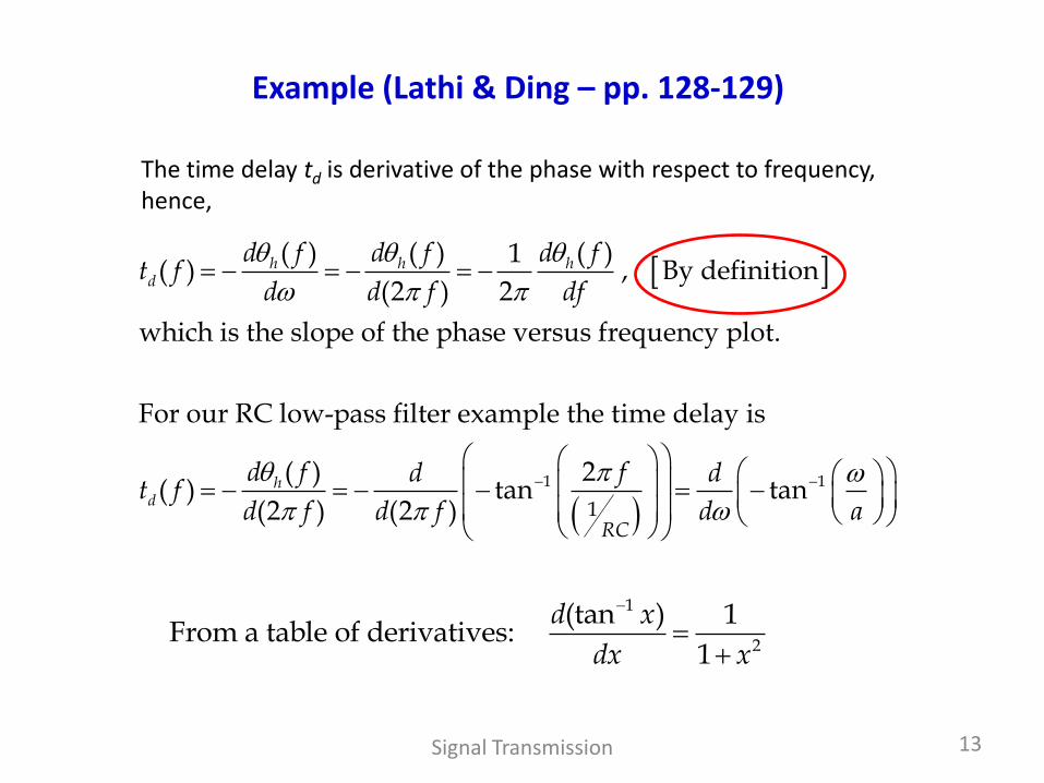
Example (Lathi & Ding – pp. 128-129)

The time delay td is derivative of the phase with respect to frequency, hence,

1

2

(tan ) 1From a table of derivatives:

1

d x

dx x

1

1

( ) ( ) ( )1( ) , By definition

(2 ) 2

which is the slope of the phase versus frequency plot.

For our RC low-pass filter example the time delay is

( ) 2( ) tan

(2 ) (2 )

h h hd

hd

d f d f d ft f

d d f df

d f fdt f

d f d f

1tan

RC

d

d a

Signal Transmission 14

Example (Lathi & Ding – pp. 128-129)

1

2

2 22

2 22

1

1

1

( ) 2( ) tan

(2 ) (2 )

21

1 1( )

1(2 ) 1 (2 )21

1( )

1 (2 )1 (2 )

Of course, for very low frequencies:

( )

hd

d

d

d

RC

RC

RC

d f fdt f

d f d f

fd

RCt fd f ff RCRC

RCRCt ffRCf

RC

t f 1 1for 2

RC f aRCa

15 Signal Transmission

Low-Pass Filter Example (Lathi & Ding)

Plot from page 129 of Lathi & Ding:

Slope is - td

Amplitude response within 2% of peak value

1aRC

(constant phase shift asymptote)

16 Signal Transmission

Example (Lathi & Ding – page 129)

( )dt f

1

a

2 f a0

1RC

a

17 Signal Transmission

Ideal Filter versus Practical Filter

The signal g(t) is transmitted without distortion, but has a time delay of td.

1

2

2

( ) and ( ) 2 ;2

( ) and2

( ) 2 sinc 2 ( )2

h d

d

d

d

j ft

j ft

fH f f ft

B

fH f

B

fh t F B B t t

B

e

e

Lathi & Ding; Page 130

dtBB

( )H f ( )h t

( ) 2h df ft

1

2B

Violates causality

f

t

1

Brick filter

18 Signal Transmission

Ideal Filter versus Practical Filter – II

Impulse response h(t) is response to impulse (t) applied at time t = 0.

The ideal filter on the previous slide is noncausal unrealizable . Practical approach to filter design is to cutoff h(t) for t < 0. A good approximation if td is large (td approaches infinity for ideal filter).

Many different practical non-ideal filters exist:

ˆ( ) ( ) ( )h t h t u t

Butterworth Chebyshev I

Chebyshev II Elliptic

Signal Transmission 19

Nth order

Butterworth Filter (Maximally Flat Magnitude)

(nth order filter)

Signal Transmission 20

Butterworth Filter (Maximally Flat Magnitude)

Sallen–Key topology

Cauer topology

22

2

(0)( )

1

n

C

HH j

Unit circle

Re(s)

Im(s)

Signal Transmission 21

Butterworth Filter Impulse Response

( )h t

( )H f

( )h f

Fourth-order filter

Lathi & Ding; Page 133

Signal Transmission 22

Comparing Butterworth, Chebyshev & Bessel Filters

http://www.analog.com/library/analogDialogue/archives/43-09/EDCh%208%20filter.pdf?doc=ADA4666-2.pdf

h(t)

Unit step response

|H(f)| |H(f)|

Unit impulse response

Signal Transmission 23

Phase Delay versus Group (Envelope) Delay

0

0

0

at one frequency

over a frequency band

Phase response of ( ) is ( ), therefore

( )Phase delay ( ) is ,

2

( )Group delay ( )

(2 )

h

hd

hgrp

f

H f f

ft and

f

d ft

d f

Input:

( ) ( ) cos(2 )

Output:

( ) ( ) ( ) cos(2 ( ) )grp d

x t A t ft

y t H f A t t f t t

Envelope

Signal Transmission 24

Group (Envelope) Delay

Group delay is an important way to describe a filter's pass band characteristics.

Consider a simple example of a square wave, which as you know, is composed of a large group of frequency components. A square wave is square only because its frequency components are in proper phase alignment with one another. If we pass a square wave through a network and expect it to remain square, then we need to ensure that the device doesn't misalign these frequency components.

Group delay is:

(1) A measure of a network’s phase distortion. (2) The transit time of a signal through a device versus frequency. (3) The derivative of the device's phase characteristic with respect to frequency (mathematical statement).

Signal Transmission 25

Channel Impairments (Overview)

• Linear distortion caused by impulse response. H(f) attenuates and phase shifts the signal.

• Nonlinear distortion (e.g., such as from clipping)

• Random Noise (independent or signal dependent)

• Interference from other transmissions or sources

• Self interference & ISI (from reflections or multipath)

( ) ( ) ( ) ( ) ( ) ( )y t h t g t Y f H f G f

( )

p

p

x

x t

x

( )

( )

( )

p

p p

p

x t x

x x t x

x t x

( )y t

ISI is intersymbol interference

Signal Transmission 26

Pulse Distortion in a Sine-Squared Pulse

Input pulse

Input pulse Input pulse

Output pulse

Output pulse

Output pulse

(a) Amplitude-frequency distortion and phase-frequency distortion

(b) Amplitude-frequency distortion (c) Phase-frequency distortion

http://users.tpg.com.au/users/ldbutler/Measurement_Distortion.htm

This is typically what pulse distortion looks like in channels.