signals and sampling - computer science and...

Signals and Sampling

Chapter 7 of “Physically Based Rendering” by Pharr&Humphreys

Chapter 7

2

7.1 Sampling Theory

7.2 Image Sampling Interface

7.3 Stratified Sampling

7.4 Low-Discrepancy Sampling

7.5 Best-Candidate Sampling Patterns

7.6 Image Reconstruction

Chapter 14.10 of “CG: Principles & Practice” by Foley, van Dam et al.Chapter 4, 5, 8, 9, 10 in “Principles of Digital Image Synthesis,” by A. GlassnerChapter 4, 5, 6 of “Digital Image Warping” by WolbergChapter 2, 4 of “Discrete-Time Signal Processing” by Oppenheim, Shafer

Additional Reading

Motivation

• Real World - continuous• Digital (Computer) world - discrete• Typically we have to either:

– create discrete data from continuous or (e.g. rendering/ray-tracing, illumination models, morphing)

– manipulate discrete data (textures, surface description, image processing,tone mapping)

Motivation

• Artifacts occurring in sampling - aliasing:– Jaggies– Moire– Flickering small objects– Sparkling highlights– Temporal strobing

• Preventing these artifacts - Antialiasing

Motivation

Convolution withbox filter

Convolution withtent filter

Engineering approach:nearest neighbor:

linear filter:

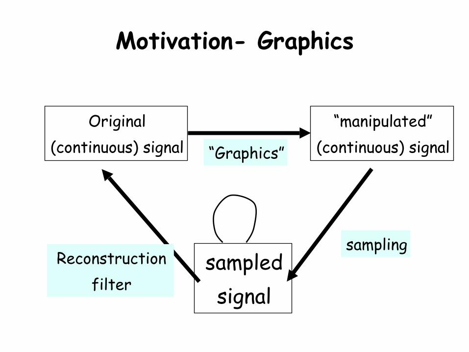
Original(continuous) signal

“manipulated”(continuous) signal

sampledsignal

“Graphics”

samplingReconstruction

filter

Motivation- Graphics

“System” orAlgorithm

Multiplication with“shah” function

Motivation

Engineering approach:• black-box

• discretization:


Convolution

• How can we characterize our “black box”?• We assume to have a “nice” box/algorithm:

– linear– time-invariant

• then it can be characterized through the response to an “impulse”:

• Impulse:

• discrete impulse:

• Finite Impulse Response (FIR) vs.• Infinite Impulse Response (IIR)

Convolution (2)

• An arbitrary signal x[k] can be written as:

• Let the impulse response be h[k]:


δ[k] h[k]

Convolution (3)


x[k] y[k]

IIR - N=inf.FIR - N<inf.

Convolution (4)• for a time-invariant system h[k-n] would

be the impulse response to a delayed impulse d[k-n]

• hence, if y[k] is the response of our system to the input x[k] (and we assume a linear system):

• Let’s look at a special input sequence:

• then:

Fourier Transforms

• Hence is an eigen-function and H(ω) its eigenvalue

• H(ω) is the Fourier-Transform of the h[n] and hence characterizes the underlying system in terms of frequencies

• H(ω) is periodic with period 2π• H(ω) is decomposed into

– phase (angle) response– magnitude response

Fourier Transforms (2)

Properties

• Linear• scaling• convolution• Multiplication

• Differentiation

• delay/shift

• Parseval’s Theorem

• preserves “Energy” - overall signal content

Properties (2)

FourierTransform

AverageFilter

Box/SincFilter

Transforms Pairs

samplingT 1/T

Transform Pairs - Shah

• Sampling = Multiplication with a Shah function:

• multiplication in spatial domain = convolution in the frequency domain

• frequency replica of primary spectrum(also called aliased spectra)

LinearFilter

GaussianFilter

derivativeFilter

Transforms Pairs (2)

Original function Sampled function

ReconstructedFunction

Acquisition

Reconstruction

Re-sampled functionResampling

General Process

Spatial Domain:

Mathematically:f(x)*h(x)

Frequency Domain:

Evaluated at discrete points (sum)

• Multiplication:• Convolution:

How? - Reconstruction

online demo

Sampling Theorem

• A signal can be reconstructed from its samples without loss of information if the original signal has no frequencies above 1/2 of the sampling frequency

• For a given bandlimited function, the rate at which it must be sampled is called the Nyquist frequency

Given

Needed

2D 1DGiven

Needed

Example

Nearest neighbor Linear Interpolation

Example

Acquisition

Reconstruction

Resampling

Original function Sampled function

ReconstructedFunction Re-sampled function

General Process -Frequency Domain

Pre-Filtering

Acquisition

Reconstruction

Original function Band-limited function

SampledFunction Reconstructed function

Pre-Filtering

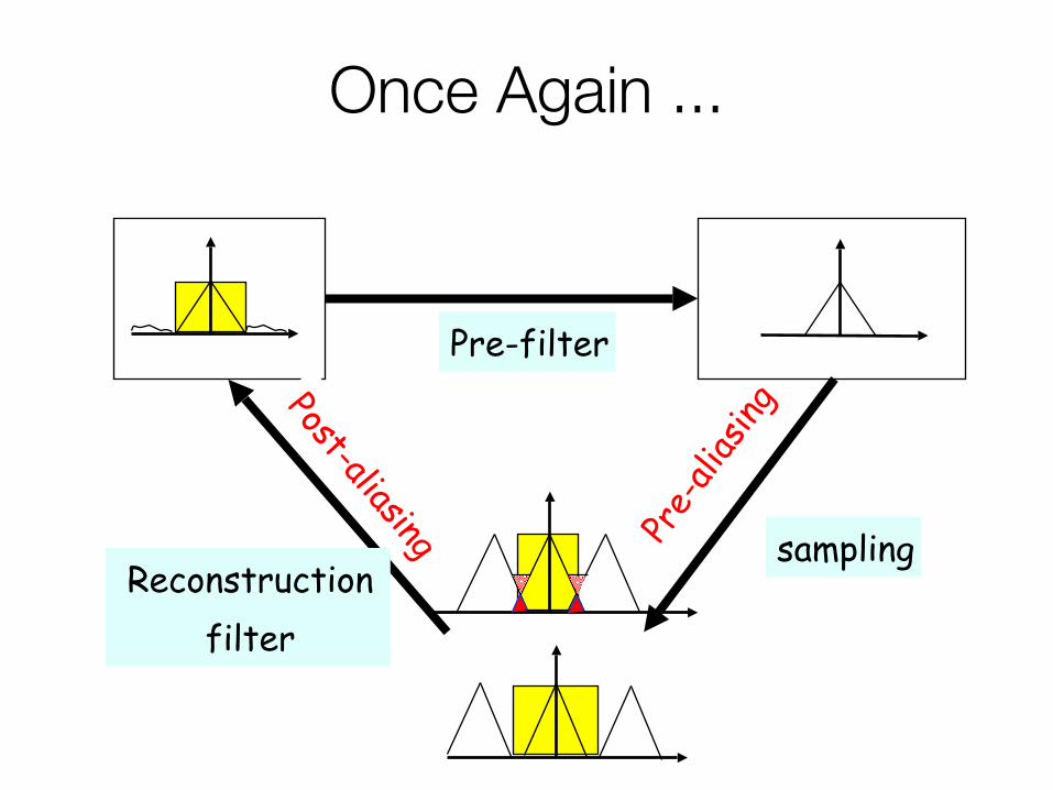
Pre-

alias

ing

Pre-filter

samplingReconstruction

filter

Post-aliasing

Once Again ...

Spatial domain Frequency domain

x

*

*

x

Pipeline - Example


x

x

*

*

Pipeline - Example (2)


x*

Pipeline - Example (3)

• Non-bandlimited signal

• Low sampling rate (below Nyquist)

• Non perfect reconstruction

Sources of Aliasing

sampling

sampling

Aliasing

Bandlimited

Spatial Domain:• convolution is exact

Frequency Domain:• cut off freq. replica

Interpolation

Derivatives

Spatial Domain:• convolution is exact

Frequency Domain:• cut off freq. replica

Spatial d. Frequency d.

Reconstruction Kernels

• Nearest Neighbor(Box)

• Linear

• Sinc

• Gaussian• Many others

Smoothing

Post-aliasing

Pass-band stop-band

Ideal filter

Practicalfilter

Ideal Reconstruction

• Box filter in frequency domain =• Sinc Filter in spatial domain• impossible to realize (really?)


• Use the sinc function – to bandlimit the sampled signal and remove all copies of the spectra introduced by sampling

• But:– The sinc has infinite extent and we must use

simpler filters with finite extents. – The windowed versions of sinc may introduce

ringing artifacts which are perceptually objectionable.

Reconstructing with Sinc

π

Low-passfilter

π

band-passfilter

π

high-passfilter


– Realizable filters do not have sharp transitions; also have ringing in pass/stop bands

T

?

Higher Dimensions?

• Design typically in 1D• extensions to higher dimensions (typically):

– separable filters– radially symmetric filters– limited results

• research topic

Possible Errors

• Post-aliasing– reconstruction filter passes frequencies beyond the

Nyquist frequency (of duplicated frequency spectrum) => frequency components of the original signal appear in the reconstructed signal at different frequencies

• Smoothing– frequencies below the Nyquist frequency are attenuated

• Ringing (overshoot)– occurs when trying to sample/reconstruct discontinuity

• Anisotropy– caused by not spherically symmetric filters

Aliasing vs. Noise

Antialiasing

• Antialiasing = Preventing aliasing• 1. Analytically pre-filter the signal

– Solvable for points, lines and polygons– Not solvable in general (e.g. procedurally

defined images)• 2. Uniform supersampling and resample• 3. Nonuniform or stochastic sampling

Uniform Supersampling

• Increasing the sampling rate moves each copy of the spectra further apart, potentially reducing the overlap and thus aliasing

• Resulting samples must be resampled (filtered) to image sampling rate

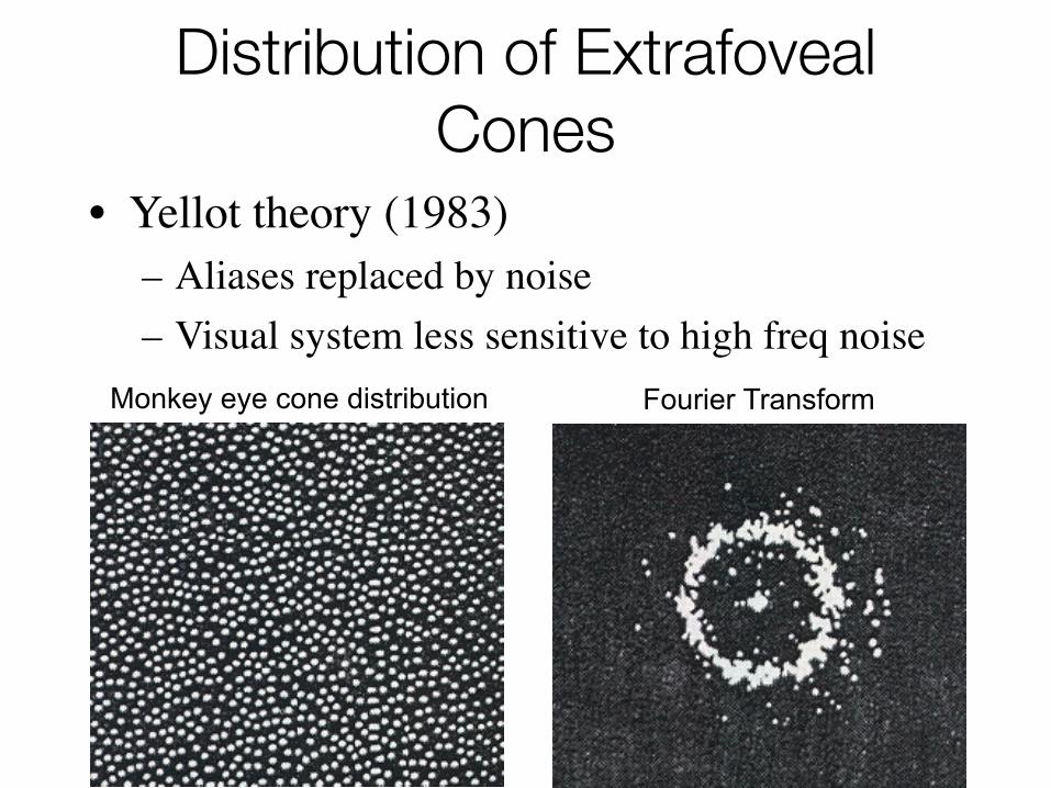
Distribution of Extrafoveal Cones

• Yellot theory (1983)– Aliases replaced by noise– Visual system less sensitive to high freq noise

Monkey eye cone distribution Fourier Transform

Non-Uniform Sampling - Intuition

• Uniform sampling– The spectrum of uniformly spaced samples is also a set

of uniformly spaced spikes– Multiplying the signal by the sampling pattern

corresponds to placing a copy of the spectrum at each spike (in freq. space)

– Aliases are coherent, and very noticeable• Non-uniform sampling

– Samples at non-uniform locations have a different spectrum; a single spike plus noise

– Sampling a signal in this way converts aliases into broadband noise

– Noise is incoherent, and much less objectionable

Non-Uniform Sampling -Patterns

• Poisson– Pick n random points in sample space

• Uniform Jitter– Subdivide sample space into n regions

• Poisson Disk– Pick n random points, but not too close

Poisson Disk Sampling

Fourier DomainSpatial Domain

Uniform Jittered Sampling

Fourier DomainSpatial Domain

Non-Uniform Sampling - Patterns

• Spectral characteristics of these distributions:– Poisson: completely uniform (white noise).

High and low frequencies equally present– Poisson disc: Pulse at origin (DC component of

image), surrounded by empty ring (no low frequencies), surrounded by white noise

– Jitter: Approximates Poisson disc spectrum, but with a smaller empty disc.

Stratified Sampling

• Put at least one sample in each strata• Multiple samples in strata do no good• Also have samples far away from each

other

• Graphics: jittering

Stratification

• OR – Split up the integration domain in N disjoint

sub-domains or strata– Evaluate the integral in each of the sub-

domains separately with one or more samples. • More precisely:

Stratification

More Jittered Sequences

Jitter

• Place samples in the grid• Perturb the samples up to 1/2 width or

height

Exact – 256 samples/pixel Jitter with 1 sample/pixel

1 sample/pixel Jitter with 4 samples/pixel

Texture Example

Multiple Dimensions

• Too many samples• 1D• 2D 3D

Jitter Problems

• How to deal with higher dimensions?– Curse of dimensionality– D dimensions means ND “cells” (if we use a

separable extension)• Solutions:

– We can look at each dimension independently– We can either look in non-separable geometries– Latin Hypercube (or N-Rook) sampling

Multiple Dimensions

• Make (separate) strata for each dimension • Randomly associate strata among each

other• Ensure good sample “distribution”

– Example: 2D screen position; 2D lens position; 1D time

Optimal sampling lattices

• Dividing space up into equal cells doesn’t have to be on a Cartesian lattices

• In fact - Cartesian is NOT the optimal way how to divide up space uniformly

Cartesian Hexagonal

Optimal sampling lattices

• We have to deal with different geometry• 2D - hexagon• 3D - truncated octahedron

• Distributing n samples in D dimensions, even if n is not a power of D

• Divide each dimension in n strata• Generate a jittered sample in each of the n

diagonal entries• Random shuffle in each dimension

Latin Hypercubes - N-Rooks

Stratification - problems

• Clamping (LHS helps)• Could still have large

empty regions

• Other geometries,e.g. stratify circlesor spheres?

}

How good are the samples ?

• How can we evaluate how well our samples are distributed?– No “holes”– No clamping

• Well distributed patterns have low discrepancy– Small = evenly distributed– Large = clustering

• Construct low discrepancy sequence

•

••

• • •

•• •

• •••

•

•

•

• •• •

• •

V

n points

N points

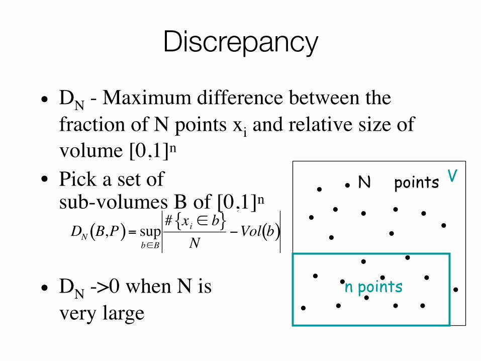
Discrepancy

• DN - Maximum difference between the fraction of N points xi and relative size of volume [0,1]n

• Pick a set ofsub-volumes B of [0,1]n

• DN ->0 when N isvery large

•

••

• • •

•• •

• •••

•

•

•

• •• •

• •

V

n points

N points

Discrepancy

• Examples of sub-volumes B of [0,1]d:– Axis-aligned– Share a corner at the origin (star

discrepancy)• Best discrepancy that has

been obtained in ddimensions:

Discrepancy• How to create low-discrepancy sequences?

– Deterministic sequences!! Not random anymore

– Also called pseudo-random– Advantage - easy to compute

• 1D:

Pseudo-Random Sequences

• Radical inverse– Building block for high-D sequences– “inverts” an integer given in base b

• Most simple sequence• Uses radical inverse of base 2• Achieves minimal

possible discrepancyi binary radical xi

form of i inverse0 0 0.0 01 1 0.1 0.52 10 0.01 0.253 11 0.11 0.754 100 0.001 0.1255 101 0.101 0.6256 110 0.011 0.375

0 12 34

Van Der Corput Sequence

Halton • Can be used if N is not known in advance• All prefixes of a sequence are well

distributed• Use prime number bases for each

dimension• Achieves best possible discrepancy

Hammersley Sequences

• Similar to Halton• Need to know total number of samples in

advance• Better discrepancy than Halton

Hammersley Sequences

Folded Radical Inverse

• Hammersley-Zaremba• Halton-Zaremba• Improves discrepancy

Examples

(t,m,d) nets

• The most successful constructions of low-discrepancy sequences are based on (t,m,d)-nets and (t,d)-sequences.

• Basis b; • Is a point set in [0,1]d consisting of bm

points, such that every box

of volume bt-m contains bt points

(t,d) Sequences

• (t,m,d)-Nets ensures, that all samples are uniformly distributed for any integer subdivision of our space.

• (t,d)-sequence is a sequence xi of points in [0,1]d such that for all integers and m>t, the point set

is a (t,m,d)-net in base b.• The number t is the quality parameter. Smaller

values of t yield more uniform nets and sequences because b-ary boxes of smaller volume still contain points.

(0,2) Sequences

• Used in pbrt for the Low-discrepancy sampler

• Base 2

Practical Issues

• Create one sequence• Create new ones from the first sequence by

“scrambling” rows and columns• This is only possible for (0,2) sequences,

since they have such a nice property (the “n-rook” property)

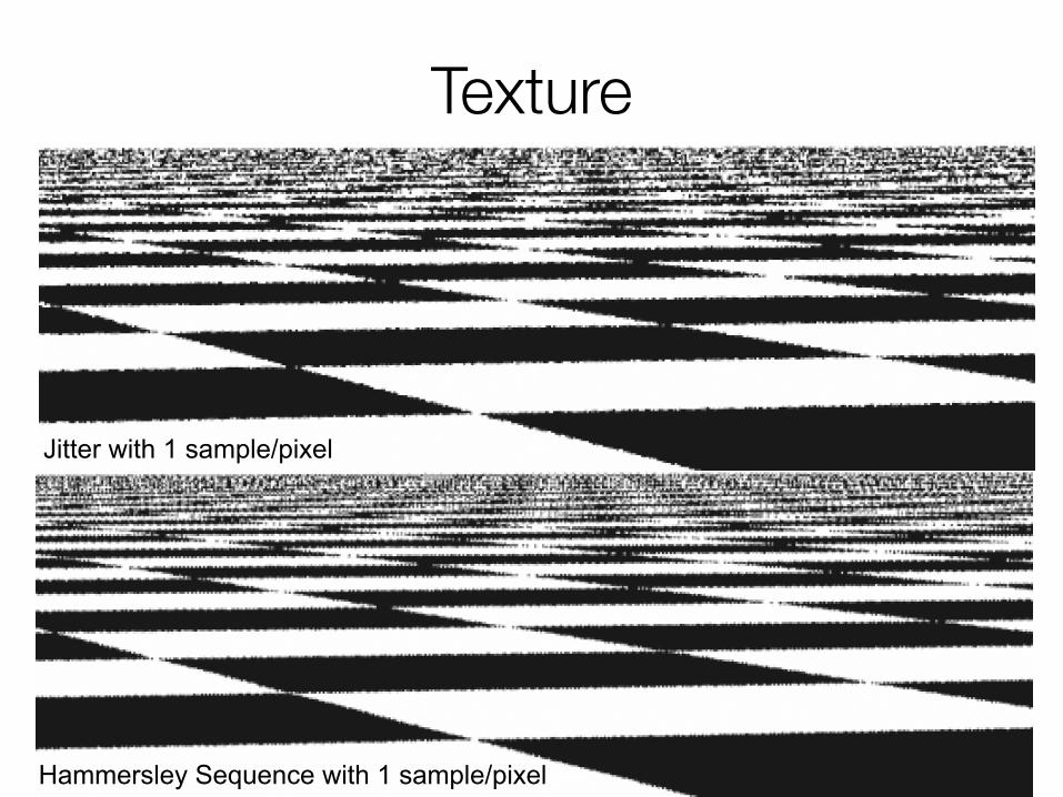
Texture

Jitter with 1 sample/pixel

Hammersley Sequence with 1 sample/pixel

Best-Candidate Sampling

• Jittered stratification – Randomness (inefficient)– Clustering problems– Undersampling (“holes”)

• Low Discrepancy Sequences– Still (visibly) aliased

• “Ideal”: Poisson disk distribution– too computationally expensive

• Best Sampling - approximation to Poisson disk

Poisson Disk

• Comes from structure of eye – rods and cones• Dart Throwing• No two points are closer than a threshold• Very expensive• Compromise – Best Candidate Sampling

– Compute pattern which is reused by tiling the image plane (translating and scaling).

– Toroidal topology– Effects the distance between points

on top to bottom


Jittered

Poisson Disk Best Candidate

Texture

TextureJitter with 1 sample/pixel Best Candidate with 1 sample/pixel

Jitter with 4 sample/pixel Best Candidate with 4 sample/pixel

Next

• Probability Theory• Monte Carlo Techniques• Rendering Equation

signals and sampling - computer science and...

Documents