Signals and Systems

Lecture 10 Tuesday 21st November 2017

DR TANIA STATHAKI READER (ASSOCIATE PROFFESOR) IN SIGNAL PROCESSING IMPERIAL COLLEGE LONDON

• We have seen that a LTI system’s response to an everlasting

exponential 𝑥 𝑡 = 𝑒𝑠𝑡 is 𝐻(𝑠)𝑒𝑠𝑡. We represent such input-output pair

as:

𝑒𝑠𝑡 ⇒ 𝐻(𝑠)𝑒𝑠𝑡

• Instead of using a complex frequency, we set 𝑠 = 𝑗𝜔. This yields:

𝑒𝑗𝜔𝑡 ⇒ 𝐻(𝑗𝜔)𝑒𝑗𝜔𝑡 cos 𝜔𝑡 = Re{𝑒𝑗𝜔𝑡} ⇒ Re{𝐻(𝑗𝜔)𝑒𝑗𝜔𝑡}

• It is often better to express 𝐻(𝑗𝜔) in polar form as:

𝐻 𝑗𝜔 = 𝐻 𝑗𝜔 𝑒𝑗∠𝐻 𝑗𝜔

• Therefore,

cos 𝜔𝑡 ⇒ 𝐻 𝑗𝜔 cos[𝜔𝑡 + ∠𝐻 𝑗𝜔 ]

𝐻 𝑗𝜔 : Frequency response

𝐻 𝑗𝜔 : Amplitude response

∠𝐻 𝑗𝜔 : Phase response

Frequency response of a LTI system to an everlasting exponential

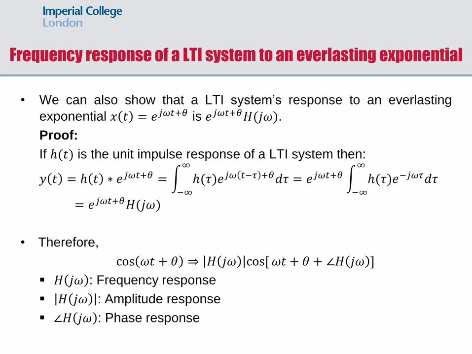
• We can also show that a LTI system’s response to an everlasting

exponential 𝑥 𝑡 = 𝑒𝑗𝜔𝑡+𝜃 is 𝑒𝑗𝜔𝑡+𝜃𝐻(𝑗𝜔).

Proof:

If ℎ(𝑡) is the unit impulse response of a LTI system then:

𝑦 𝑡 = ℎ 𝑡 ∗ 𝑒𝑗𝜔𝑡+𝜃 = ℎ(𝜏∞

−∞

)𝑒𝑗𝜔 𝑡−𝜏 +𝜃𝑑𝜏 = 𝑒𝑗𝜔𝑡+𝜃 ℎ(𝜏∞

−∞

)𝑒−𝑗𝜔𝜏𝑑𝜏

= 𝑒𝑗𝜔𝑡+𝜃𝐻(𝑗𝜔)

• Therefore,

cos 𝜔𝑡 + 𝜃 ⇒ 𝐻 𝑗𝜔 cos[𝜔𝑡 + 𝜃 + ∠𝐻 𝑗𝜔 ]

𝐻 𝑗𝜔 : Frequency response

𝐻 𝑗𝜔 : Amplitude response

∠𝐻 𝑗𝜔 : Phase response

Frequency response of a LTI system to an everlasting exponential

• Find the frequency response (amplitude and phase response) of a

system with transfer function:

𝐻 𝑠 =𝑠 + 0.1

𝑠 + 5

Then find the system’s response 𝑦(𝑡) for inputs 𝑥 𝑡 = cos2𝑡 and

𝑥 𝑡 = cos(10𝑡 − 50o).

• We substitute 𝑠 = 𝑗𝜔. Then, we obtain 𝐻 𝑗𝜔 =𝑗𝜔+0.1

𝑗𝜔+5.

Amplitude response: 𝐻 𝑗𝜔 =𝜔2+0.01

𝜔2+25 .

Phase response: ∠𝐻 𝑗𝜔 = Φ 𝜔 = tan−1𝜔

0.1− tan−1

𝜔

5.

Frequency response example

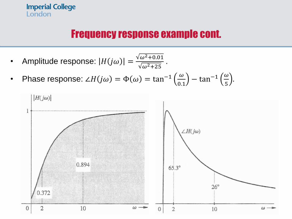
• Amplitude response: 𝐻 𝑗𝜔 =𝜔2+0.01

𝜔2+25 .

• Phase response: ∠𝐻 𝑗𝜔 = Φ 𝜔 = tan−1𝜔

0.1− tan−1

𝜔

5.

Frequency response example cont.

• For input 𝑥 𝑡 = cos2𝑡 we have:

Amplitude response: 𝐻 𝑗2 =22+0.01

22+25= 0.372.

Phase response: ∠𝐻 𝑗2 = Φ 𝑗2 = tan−12

0.1− tan−1

2

5= 65.3o.

• Therefore,

𝑦 𝑡 = 0.372cos(2𝑡 + 65.3o)

Frequency response example cont.

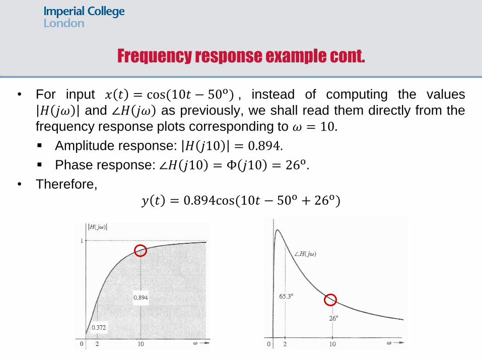
• For input 𝑥 𝑡 = cos(10𝑡 − 50o) , instead of computing the values

𝐻 𝑗𝜔 and ∠𝐻 𝑗𝜔 as previously, we shall read them directly from the

frequency response plots corresponding to 𝜔 = 10.

Amplitude response: 𝐻 𝑗10 = 0.894.

Phase response: ∠𝐻 𝑗10 = Φ 𝑗10 = 26o.

• Therefore,

𝑦 𝑡 = 0.894cos(10𝑡 − 50o + 26o)

Frequency response example cont.

• The transfer function of an ideal delay is 𝐻 𝑠 = 𝑒−𝑠𝑇 (proven previously).

• Therefore,

Amplitude response: 𝐻(𝑗𝜔) = 𝑒−𝑗𝜔𝑇 = 1.

Phase response: ∠𝐻 𝑗𝜔 = Φ 𝑗𝜔 = −𝜔𝑇.

• Therefore:

Delaying a signal by 𝑇 has no effect

on its amplitude.

It introduces a linear phase shift

with a gradient of −𝑇.

The quantity −𝑑Φ 𝜔

𝑑𝜔= 𝜏𝑔 = 𝑇 is

known as Group Delay.

Frequency response of a system that causes delay of 𝑇 sec

• The transfer function of an ideal differentiator is 𝐻 𝑠 = 𝑠.

• Therefore,

Frequency response: 𝐻 𝑗𝜔 = 𝑗𝜔.

Amplitude response: 𝐻(𝑗𝜔) = 𝜔.

Phase response: ∠𝐻 𝑗𝜔 =𝜋

2.

(Recall that 𝑗 = 𝑒𝑗𝜋

2)

• This agrees with: 𝑑

𝑑𝑡cos𝜔𝑡 = −𝜔sin𝜔𝑡 = 𝜔cos(𝜔𝑡 +

𝜋

2)

• That is why differentiator is not

a nice component to work with;

it amplifies high frequency

components (i.e., noise).

Frequency response of an ideal differentiator

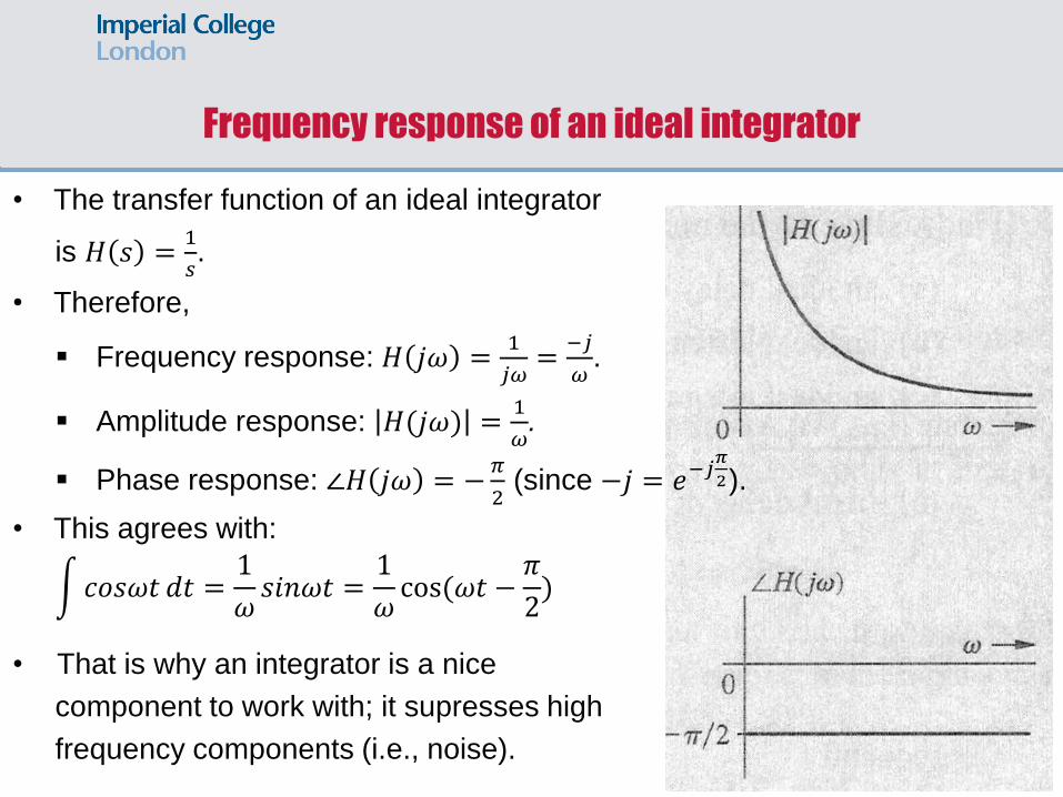
• The transfer function of an ideal integrator

is 𝐻 𝑠 =1

𝑠.

• Therefore,

Frequency response: 𝐻 𝑗𝜔 =1

𝑗𝜔=−𝑗

𝜔.

Amplitude response: 𝐻(𝑗𝜔) =1

𝜔.

Phase response: ∠𝐻 𝑗𝜔 = −𝜋

2 (since −𝑗 = 𝑒−𝑗

𝜋

2).

• This agrees with:

𝑐𝑜𝑠𝜔𝑡 𝑑𝑡 =1

𝜔𝑠𝑖𝑛𝜔𝑡 =

1

𝜔cos(𝜔𝑡 −

𝜋

2)

• That is why an integrator is a nice

component to work with; it supresses high

frequency components (i.e., noise).

Frequency response of an ideal integrator

• Consider a system with transfer function:

𝐻 𝑠 =𝐾(𝑠+𝑎1)(𝑠+𝑎2)

𝑠(𝑠+𝑏1)(𝑠2+𝑏2𝑠+𝑏3)

= 𝐾𝑎1𝑎2

𝑏1𝑏3

(𝑠

𝑎1+1)(

𝑠

𝑎2+1)

𝑠(𝑠

𝑏1+1)(

𝑠2

𝑏3+𝑏2𝑏3𝑠+1)

• The poles are the roots of the denominator polynomial. In this case, the poles of the system are 𝑠 = 0, 𝑠 = −𝑏1 and the solutions of the quadratic

𝑠2 + 𝑏2𝑠 + 𝑏3 = 0

which we assume to form a complex conjugate pair.

• The zeros are the roots of the numerator polynomial. In this case, the zeros of the system are 𝑠 = −𝑎1, 𝑠 = −𝑎2.

Bode Plots

Asymptotic behaviour of amplitude and phase response

• Now let 𝑠 = 𝑗𝜔.The amplitude response 𝐻(𝑗𝜔) can be rearranged as:

𝐻(𝑗𝜔) = 𝐾𝑎1𝑎2

𝑏1𝑏3

1+𝑗𝜔

𝑎11+𝑗𝜔

𝑎2

𝑗𝜔 1+𝑗𝜔

𝑏11+𝑗

𝑏2𝜔

𝑏3+(𝑗𝜔)2

𝑏3

• We express the above in decibel (i.e., 20log(∙)):

20log 𝐻(𝑗𝜔) = 20log 𝐾𝑎1𝑎2𝑏1𝑏3

+20log 1 +𝑗𝜔

𝑎1+ 20log 1 +

𝑗𝜔

𝑎2

−20 log 𝑗𝜔 − 20log 1 +𝑗𝜔

𝑏1− 20 log 1 + 𝑗

𝑏2𝜔

𝑏3+(𝑗𝜔)2

𝑏3

• By imposing a log operation the amplitude response (in dB) is broken

into building block components that are added together.

• We have three types of building block terms: A term 𝑗𝜔, a first order

term 1 +𝑗𝜔

𝑎 and a second order term with complex conjugate roots.

Bode Plots

Asymptotic behaviour of amplitude and phase response

• They are desirable in several applications, where the variables considered

have a very large range of values.

• The above is particularly true in frequency response amplitude plots since

we require to plot values from 10−6 to 106 or higher.

• A plot of such a large range on a linear scale will bury much of the useful

information at lower frequencies.

• In humans the relationship between stimulus and perception is logarithmic.

This means that if a stimulus varies as a geometric progression (i.e.,

multiplied by a fixed factor), the corresponding perception is altered in

an arithmetic progression (i.e., in additive constant amounts). For

example, if a stimulus is tripled in strength (i.e., 3 x 1), the

corresponding perception may be two times as strong as its original

value (i.e., 1 + 1).

There is a theory behind the above observations developed by Weber

and Frechner.

Advantages of logarithmic units

• A pole at the origin gives rise to the amplitude term −20 log 𝑗𝜔 = −20 log𝜔

This function can be plotted as function of 𝜔.

We can effect further simplification by using the logarithmic function for the

variable 𝜔 itself. Therefore, we define 𝑢 = log𝜔.

• Therefore, −20 log𝜔 = −20𝑢.

This is a straight line with a slope of −20.

A ratio of 10 in 𝜔 is called a decade. If 𝜔2 = 10𝜔1 then

𝑢2 = log𝜔2 = log10𝜔1 = log10 + log𝜔1 = 1 + log𝜔1 = 1 + 𝑢1.

A ratio of 2 in 𝜔 is called an octave. If 𝜔2 = 2𝜔1 then

𝑢2 = log𝜔2 = log2𝜔1 = log2 + log𝜔1 = 0.301 + log𝜔1 = 0.301 + 𝑢1

• Based on the above, equal increments in 𝑢 are equivalent to equal ratios in

𝜔.

• The amplitude plot has a slope of −20𝑑B/ decade or −20 0.301 =− 6.02𝑑B/octave.

• The amplitude plot crosses the 𝜔 axis at 𝜔 = 1, since 𝑢 = log𝜔 = 0 for 𝜔 = 1.

Bode plots – a pole at the origin: amplitude

• A zero at the origin gives rise to the term 20 log 𝑗𝜔 = 20 log𝜔.

• Therefore, 20 log𝜔 = 20𝑢.

• The amplitude plot has a slope of 20𝑑B/ decade or 20 0.301 =6.02𝑑B/octave.

• The amplitude plot for a zero at the origin is a mirror image about the 𝜔

axis of the plot for a pole at the origin.

Amplitudes of a pole and a zero at the origin

Bode plots – a zero at the origin: amplitude

• The log amplitude of a first order pole at −𝑎 is −20log 1 +𝑗𝜔

𝑎.

𝜔 ≪ 𝑎 ⇒ −20log 1 +𝑗𝜔

𝑎≈ −20log1 = 0

𝜔 ≫ 𝑎 ⇒ −20log 1 +𝑗𝜔

𝑎≈ −20log(

𝜔

𝑎) = −20log𝜔 + 20log𝑎

This represents a straight line (when plotted as a function of 𝑢, the log

of 𝜔) with a slope of −20𝑑𝐵/decade or −20 0.301 = −6.02𝑑𝐵/octave.

When 𝜔 = 𝑎 the log amplitude is zero. Hence, this line crosses the 𝜔

axis at 𝜔 = 𝑎. Note that the asymptotes meet at 𝜔 = 𝑎.

• The exact log amplitude for this pole is:

−20log 1 +𝑗𝜔

𝑎= −20log 1 +

𝜔2

𝑎2

12

= −10log 1 +𝜔2

𝑎2

• The maximum error between the actual and asymptotic plots occurs at

𝜔 = 𝑎 and is −3𝑑B. The frequency 𝜔 = 𝑎 is called corner frequency or

break frequency.

Bode plots – first order pole: amplitude

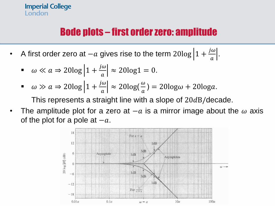
• A first order zero at −𝑎 gives rise to the term 20log 1 +𝑗𝜔

𝑎.

𝜔 ≪ 𝑎 ⇒ 20log 1 +𝑗𝜔

𝑎≈ 20log1 = 0.

𝜔 ≫ 𝑎 ⇒ 20log 1 +𝑗𝜔

𝑎≈ 20log(

𝜔

𝑎) = 20log𝜔 + 20log𝑎.

This represents a straight line with a slope of 20𝑑B/decade.

• The amplitude plot for a zero at −𝑎 is a mirror image about the 𝜔 axis

of the plot for a pole at −𝑎.

Amplitude of a pole and a zero at the origin

Bode plots – first order zero: amplitude

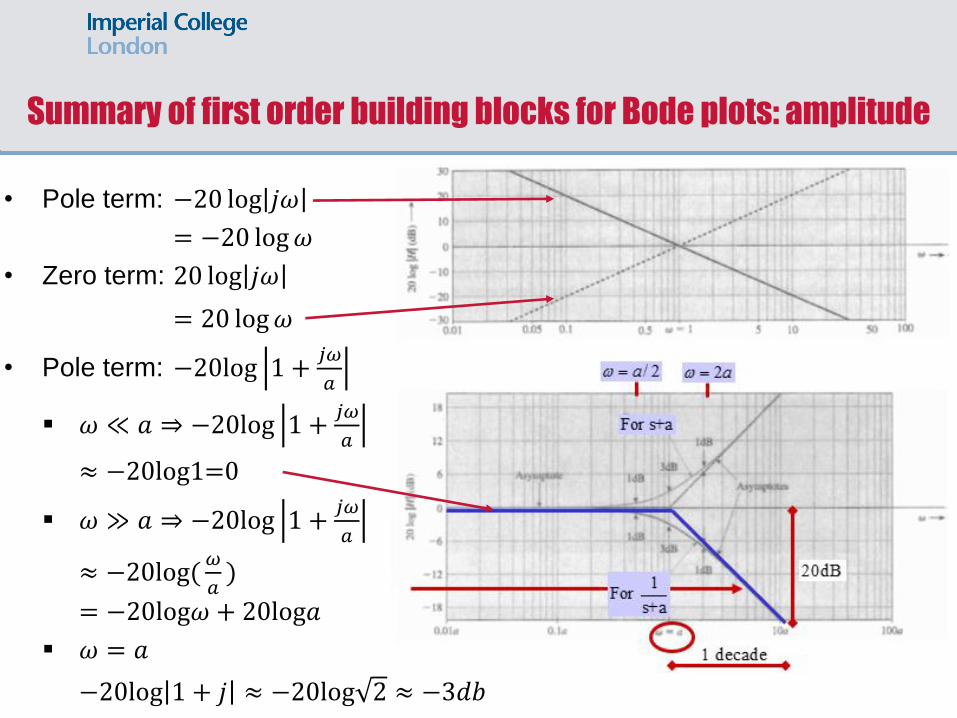
• Pole term: −20 log 𝑗𝜔

= −20 log𝜔

• Zero term: 20 log 𝑗𝜔

= 20 log𝜔

• Pole term: −20log 1 +𝑗𝜔

𝑎

𝜔 ≪ 𝑎 ⇒ −20log 1 +𝑗𝜔

𝑎

≈ −20log1=0

𝜔 ≫ 𝑎 ⇒ −20log 1 +𝑗𝜔

𝑎

≈ −20log(𝜔

𝑎)

= −20log𝜔 + 20log𝑎

𝜔 = 𝑎

−20log 1 + 𝑗 ≈ −20log 2 ≈ −3𝑑𝑏

Summary of first order building blocks for Bode plots: amplitude

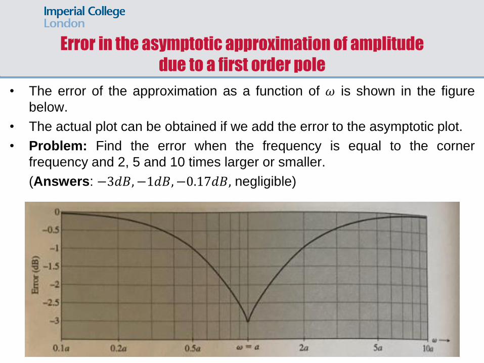
• The error of the approximation as a function of 𝜔 is shown in the figure

below.

• The actual plot can be obtained if we add the error to the asymptotic plot.

• Problem: Find the error when the frequency is equal to the corner

frequency and 2, 5 and 10 times larger or smaller.

(Answers: −3𝑑𝐵,−1𝑑𝐵,−0.17𝑑𝐵, negligible)

Error in the asymptotic approximation of amplitude

due to a first order pole

• Now consider the quadratic term: 𝑠2 + 𝑏2𝑠 + 𝑏3.

• It is quite common to express the above term as: 𝑠2 + 2𝜁𝜔𝑛𝑠 + 𝜔𝑛2.

The scalar 𝜁 is called damping factor.

The scalar 𝜔𝑛 is called natural frequency.

• The log amplitude response is:

log amplitude = −20log 1 + 2𝑗𝜁(𝜔

𝜔𝑛) + (

𝑗𝜔

𝜔𝑛)2

𝜔 ≪ 𝜔𝑛, log amplitude ≈ −20log1 = 0

𝜔 ≫ 𝜔𝑛, log amplitude ≈ −20log −(𝜔

𝜔𝑛)2 = −40log (

𝜔

𝜔𝑛)

= −40log𝜔 − 40log𝜔𝑛 = −40𝑢 − 40log𝜔𝑛

The exact log amplitude is −20log [1 − (𝜔

𝜔𝑛)2]2+4𝜁2(

𝜔

𝜔𝑛)2

1/2

Bode plots – second order pole : amplitude

• The log amplitude involves a parameter 𝜁, resulting in a different plot for

each value of 𝜁.

• It can be proven that for complex-conjugate poles 𝜁 < 1.

• For 𝜁 ≥ 1, the two poles in the second order factor are not longer

complex but real, and each of these two real poles can be dealt with as

a separate first order factor.

• The amplitude plot for a pair of complex conjugate zeros is a mirror

image about the 𝜔 axis of the plot for a pair of complex conjugate poles.

Bode plots – second order pole : amplitude

• The exact log amplitude is = −20log [1 − (𝜔

𝜔𝑛)2]2+4𝜁2(

𝜔

𝜔𝑛)2

1/2

Bode plots – second order pole : amplitude

• The error of the approximation as a function of 𝜔 is shown in the figure

below for various values of 𝜁s.

• The actual plot can be obtained if we add the error to the asymptotic

plot.

Error in the asymptotic approximation of amplitude

due to a pair of complex conjugate poles

Bode plots example: amplitude

• Consider a system with transfer function:

𝐻 𝑠 =20𝑠(𝑠 + 100)

(𝑠 + 2)(𝑠 + 10)

𝐻 𝑠 =20×100

2×10 𝑠(1+

𝑠

100)

(1+𝑠

2)(1+

𝑠

10)= 100

𝑠(1+𝑠

100)

(1+𝑠

2)(1+

𝑠

10)

• Step 1: Establish where 𝑥 − axis crosses the 𝑦 − axis.

Since the constant term is 100 = 40𝑑𝐵, 𝑥 −axis cuts the vertical axis

at 40 (i.e., relabel the horizontal axis as the 40𝑑𝐵 line).

• Step 2: For each pole and zero term draw an asymptotic plot.

We need to draw straight lines for zero terms at origin and 𝜔 =− 100.

We need to draw straight lines for pole terms at 𝜔 = −2 and

𝜔 = −10.

• Step 3: Add all the asymptotes.

• Step 4: Apply corrections if possible.

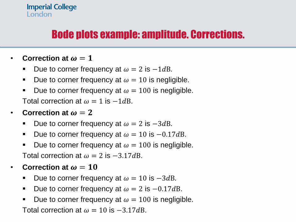
Bode plots example: amplitude. Corrections.

• Correction at 𝝎 = 𝟏

Due to corner frequency at 𝜔 = 2 is −1𝑑B.

Due to corner frequency at 𝜔 = 10 is negligible.

Due to corner frequency at 𝜔 = 100 is negligible.

Total correction at 𝜔 = 1 is −1𝑑B.

• Correction at 𝝎 = 𝟐

Due to corner frequency at 𝜔 = 2 is −3𝑑B.

Due to corner frequency at 𝜔 = 10 is −0.17𝑑B.

Due to corner frequency at 𝜔 = 100 is negligible.

Total correction at 𝜔 = 2 is −3.17𝑑B.

• Correction at 𝝎 = 𝟏𝟎

Due to corner frequency at 𝜔 = 10 is −3𝑑B.

Due to corner frequency at 𝜔 = 2 is −0.17𝑑B.

Due to corner frequency at 𝜔 = 100 is negligible.

Total correction at 𝜔 = 10 is −3.17𝑑B.

Bode plots example: amplitude. Corrections cont.

• Correction at 𝝎 = 𝟏𝟎𝟎

Due to corner frequency at 𝜔 = 100 is 3𝑑B.

Due to corner frequency at 𝜔 = 2 is negligible.

Due to corner frequency at 𝜔 = 10 is negligible.

Total correction at 𝜔 = 100 is 3𝑑B.

• Correction at intermediate points other than corner frequencies may be

considered for more accurate plots.

Bode plots example: total amplitude

• Observe now the final plot for the previous system with transfer function:

𝐻 𝑠 = 100 𝑠(1+

𝑠

100)

(1+𝑠

2)(1+

𝑠

10)

• Now consider the phase response for the earlier transfer function:

𝐻(𝑗𝜔) = 𝐾𝑎1𝑎2

𝑏1𝑏3

(1+𝑗𝜔

𝑎1)(1+

𝑗𝜔

𝑎2)

𝑗𝜔(1+𝑗𝜔

𝑏1)(1+𝑗

𝑏2𝜔

𝑏3+(𝑗𝜔)2

𝑏3)

• The phase response is:

∠𝐻 𝑗𝜔 = ∠ 1 +𝑗𝜔

𝑎1+ ∠ 1 +

𝑗𝜔

𝑎2− ∠𝑗𝜔

−∠(1 +𝑗𝜔

𝑏1) − ∠(1 + 𝑗

𝑏2𝜔

𝑏3+𝑗𝜔 2

𝑏3)

• Again, we have three types of terms.

Bode plots: phase

• A pole at the origin gives rise to the term −𝑗𝜔.

∠𝐻 𝑗𝜔 = −∠𝑗𝜔 = −90o . The phase is therefore, constant for all

values of 𝜔.

• A zero at the origin gives rise to the term 𝑗𝜔.

∠𝐻 𝑗𝜔 = ∠𝑗𝜔 = 90o. The phase plot for a zero at the origin is a

mirror image about the 𝜔 axis of the phase plot for a pole at the origin.

Bode plots – a pole or zero at the origin: phase

• A pole at −𝑎 gives rise to the term 1 +𝑗𝜔

𝑎.

∠𝐻 𝑗𝜔 = − ∠ 1 +𝑗𝜔

𝑎= −tan−1

𝜔

𝑎.

𝜔 ≪ 𝑎 ⇒ −tan−1 𝜔

𝑎≈ 0

𝜔 ≫ 𝑎 ⇒ −tan−1 𝜔

𝑎≈ −90o

• The phase plot for a zero at −𝑎 is a mirror image about the 𝜔 axis of the

phase plot for a pole at the origin.

Bode plots – a first order pole or zero: phase

• We use a three-line segment asymptotic plot for greater accuracy. The

asymptotes are:

𝜔 ≤ 𝑎/10 ⇒ 0o

𝜔 ≥ 10𝑎 ⇒ −90o

A straight line with slope −45o /decade connects the above two

asymptotes (from 𝜔 = 𝑎/10 to 𝜔 = 10𝑎) crossing the 𝜔 axis at 𝜔 = 𝑎/10.

Bode plots – a first order pole or zero: phase

• The asymptotes are very close to the real curve and the maximum error

is 5.7o.

• The actual phase can be obtained if we add the error to the asymptotic

plot.

Bode plots – a first order pole or zero: phase error

• Now consider the term:

1 + 2𝑗𝜁𝜔

𝜔𝑛+

𝑗𝜔

𝜔𝑛

2= 1 −

𝜔

𝜔𝑛

2+ 𝑗 2𝜁(

𝜔

𝜔𝑛)

∠𝐻 𝑗𝜔 = −tan−12𝜁(

𝜔𝜔𝑛)

1 − (𝜔𝜔𝑛)2

𝜔 ≪ 𝜔𝑛, ∠𝐻 𝑗𝜔 ≈ −tan−10 ≈ 0

𝜔 ≫ 𝜔𝑛, ∠𝐻 𝑗𝜔 ≈ −tan−10 ≈ −180o

• The phase involves a parameter 𝜁, resulting in a different plot for each

value of 𝜁.

Bode plots – second order complex conjugate poles : phase

• A convenient asymptote for the phase of complex conjugate poles is a

step function that is 0o for 𝜔 < 𝜔𝑛 and −180o for 𝜔 > 𝜔𝑛.

• For complex conjugate zeros, the amplitude and phase plots are mirror

images of those for complex conjugate plots.

Bode plots – second order complex conjugate poles : phase

• An error plot is shown in the figure below for various values of 𝜁.

• The actual phase can be obtained if we add the error to the asymptotic

plot.

Bode plots – second order complex conjugate poles : phase error

Bode plots example: phase

• Consider the previous system with transfer function:

𝐻 𝑠 =20𝑠(𝑠+100)

(𝑠+2)(𝑠+10)= 100

𝑠(1+𝑠

100)

(1+𝑠

2)(1+

𝑠

10)

• For the pole at 𝑠 = −2 (𝑎 = −2) the phase plot is:

𝜔 ≤2

10= 0.2 ⇒ 0o

𝜔 ≥ 10 ∙ 2 = 20 ⇒ −90o

A straight line with slope −45o /decade connects the above two

asymptotes (from 𝜔 = 0.2 to 𝜔 = 20) crossing the 𝜔 axis at 𝜔 = 0.2.

• For the pole at 𝑠 = −10 (𝑎 = −10) the phase plot is:

𝜔 ≤10

10= 1 ⇒ 0o

𝜔 ≥ 10 ∙ 10 = 100 ⇒ −90o

A straight line with slope −45o /decade connects the above two

asymptotes (from 𝜔 = 1 to 𝜔 = 100) crossing the 𝜔 axis at 𝜔 = 1.

Bode plots example: phase cont.

• Consider the previous system with transfer function:

𝐻 𝑠 =20𝑠(𝑠+100)

(𝑠+2)(𝑠+10)= 100

𝑠(1+𝑠

100)

(1+𝑠

2)(1+

𝑠

10)

• The zero at the origin causes a 90ophase shift.

• For the zero at 𝑠 = −100 (𝑎 = −100) the phase plot is:

𝜔 ≤100

10= 10 ⇒ 0o

𝜔 ≥ 10 ∙ 100 = 1000 ⇒ 90o

A straight line with slope 45o /decade connects the above two

asymptotes (from 𝜔 = 10 to 𝜔 = 1000) crossing the 𝜔 axis at 𝜔 =10.

Bode plots example: total phase cont.

• Consider the previous system with transfer function:

𝐻 𝑠 = 100 𝑠(1+

𝑠

100)

(1+𝑠

2)(1+

𝑠

10)

Relating this lecture to other courses

• You will be applying frequency response in various areas such as filters

and 2nd year control. You have also used frequency response in the 2nd

year analogue electronics course. Here we explore this as a special

case of the general concept of complex frequency, where the real part is

zero.

• You have come across Bode plots from 2nd year analogue electronics

course. Here we go deeper into where all these rules come from.

• We will apply much of what we have done so far in the frequency

domain to analyse and design some filters in the next lecture.