signals and systems with matlab
TRANSCRIPT


Signals and Systems with MATLAB R©

Won Y. Yang · Tae G. Chang · Ik H. Song ·Yong S. Cho · Jun Heo · Won G. Jeon ·Jeong W. Lee · Jae K. Kim
Signals and Systemswith MATLAB R©
123

Limits of Liability and Disclaimer of Warranty of Software
The reader is expressly warned to consider and adopt all safety precautions that mightbe indicated by the activities herein and to avoid all potential hazards. By following theinstructions contained herein, the reader willingly assumes all risks in connection withsuch instructions.
The authors and publisher of this book have used their best efforts and knowledge inpreparing this book as well as developing the computer programs in it. However, theymake no warranty of any kind, expressed or implied, with regard to the programs orthe documentation contained in this book. Accordingly, they shall not be liable for anyincidental or consequential damages in connection with, or arising out of, the readers’use of, or reliance upon, the material in this book.
Questions about the contents of this book can be mailed to [email protected] files in this book can be downloaded from the following website:
<http://wyyang53.com.ne.kr/>
MATLAB R© and Simulink R© are registered trademarks of The MathWorks, Inc. ForMATLAB and Simulink product information, please contact:
The MathWorks, Inc.3 Apple Hill DriveNatick, MA 01760-2098 USA�: 508-647-7000, Fax: 508-647-7001E-mail: [email protected]: www.mathworks.com
ISBN 978-3-540-92953-6 e-ISBN 978-3-540-92954-3DOI 10.1007/978-3-540-92954-3Springer Dordrecht Heidelberg London New York
Library of Congress Control Number: 2009920196
c© Springer-Verlag Berlin Heidelberg 2009This work is subject to copyright. All rights are reserved, whether the whole or part of the material isconcerned, specifically the rights of translation, reprinting, reuse of illustrations, recitation, broadcasting,reproduction on microfilm or in any other way, and storage in data banks. Duplication of this publicationor parts thereof is permitted only under the provisions of the German Copyright Law of September 9,1965, in its current version, and permission for use must always be obtained from Springer. Violationsare liable to prosecution under the German Copyright Law.The use of general descriptive names, registered names, trademarks, etc. in this publication does notimply, even in the absence of a specific statement, that such names are exempt from the relevant protectivelaws and regulations and therefore free for general use.
Cover design: WMXDesign GmbH, Heidelberg
Printed on acid-free paper
Springer is a part of Springer Science+Business Media (www.springer.com)

To our parents and familieswho love and support us
andto our teachers and studentswho enriched our knowledge
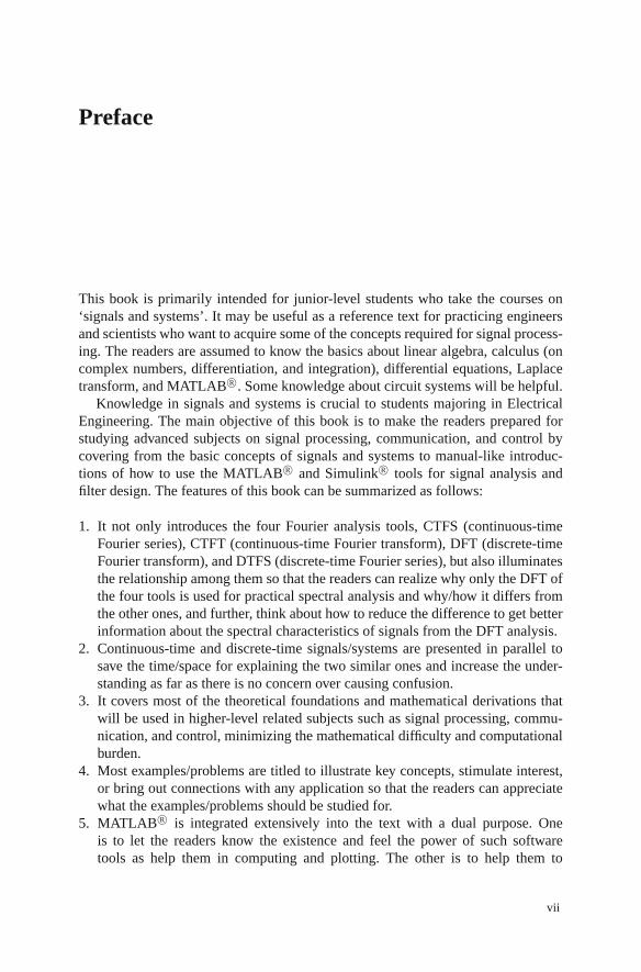
Preface
This book is primarily intended for junior-level students who take the courses on‘signals and systems’. It may be useful as a reference text for practicing engineersand scientists who want to acquire some of the concepts required for signal process-ing. The readers are assumed to know the basics about linear algebra, calculus (oncomplex numbers, differentiation, and integration), differential equations, Laplacetransform, and MATLAB R©. Some knowledge about circuit systems will be helpful.
Knowledge in signals and systems is crucial to students majoring in ElectricalEngineering. The main objective of this book is to make the readers prepared forstudying advanced subjects on signal processing, communication, and control bycovering from the basic concepts of signals and systems to manual-like introduc-tions of how to use the MATLAB R© and Simulink R© tools for signal analysis andfilter design. The features of this book can be summarized as follows:
1. It not only introduces the four Fourier analysis tools, CTFS (continuous-timeFourier series), CTFT (continuous-time Fourier transform), DFT (discrete-timeFourier transform), and DTFS (discrete-time Fourier series), but also illuminatesthe relationship among them so that the readers can realize why only the DFT ofthe four tools is used for practical spectral analysis and why/how it differs fromthe other ones, and further, think about how to reduce the difference to get betterinformation about the spectral characteristics of signals from the DFT analysis.
2. Continuous-time and discrete-time signals/systems are presented in parallel tosave the time/space for explaining the two similar ones and increase the under-standing as far as there is no concern over causing confusion.
3. It covers most of the theoretical foundations and mathematical derivations thatwill be used in higher-level related subjects such as signal processing, commu-nication, and control, minimizing the mathematical difficulty and computationalburden.
4. Most examples/problems are titled to illustrate key concepts, stimulate interest,or bring out connections with any application so that the readers can appreciatewhat the examples/problems should be studied for.
5. MATLAB R© is integrated extensively into the text with a dual purpose. Oneis to let the readers know the existence and feel the power of such softwaretools as help them in computing and plotting. The other is to help them to
vii

viii Preface
realize the physical meaning, interpretation, and/or application of such conceptsas convolution, correlation, time/frequency response, Fourier analyses, and theirresults, etc.
6. The MATLAB R© commands and Simulink R© blocksets for signal processingapplication are summarized in the appendices in the expectation of being usedlike a manual. The authors made no assumption that the readers are proficient inMATLAB R© . However, they do not hide their expectation that the readers willget interested in using the MATLAB R© and Simulink R© for signal analysis andfilter design by trying to understand the MATLAB R© programs attached to someconceptually or practically important examples/problems and be able to modifythem for solving their own problems.
The contents of this book are derived from the works of many (known orunknown) great scientists, scholars, and researchers, all of whom are deeply appre-ciated. We would like to thank the reviewers for their valuable comments andsuggestions, which contribute to enriching this book.
We also thank the people of the School of Electronic & Electrical Engineering,Chung-Ang University for giving us an academic environment. Without affectionsand supports of our families and friends, this book could not be written. Specialthanks should be given to Senior Researcher Yong-Suk Park of KETI (Korea Elec-tronics Technology Institute) for his invaluable help in correction. We gratefullyacknowledge the editorial and production staff of Springer-Verlag, Inc. includingDr. Christoph Baumann and Ms. Divya Sreenivasan, Integra.
Any questions, comments, and suggestions regarding this book are welcome.They should be sent to [email protected].
Seoul, Korea Won Y. YangTae G. Chang
Ik H. SongYong S. Cho
Jun HeoWon G. JeonJeong W. Lee
Jae K. Kim

Contents
1 Signals and Systems . . . . . . . . . . . . . . . . . . . . . . . . . . . . . . . . . . . . . . . . . . . . . 11.1 Signals . . . . . . . . . . . . . . . . . . . . . . . . . . . . . . . . . . . . . . . . . . . . . . . . . . . 2
1.1.1 Various Types of Signal . . . . . . . . . . . . . . . . . . . . . . . . . . . . . . 21.1.2 Continuous/Discrete-Time Signals . . . . . . . . . . . . . . . . . . . . . 21.1.3 Analog Frequency and Digital Frequency . . . . . . . . . . . . . . . . 61.1.4 Properties of the Unit Impulse Function
and Unit Sample Sequence . . . . . . . . . . . . . . . . . . . . . . . . . . . 81.1.5 Several Models for the Unit Impulse Function . . . . . . . . . . . . 11
1.2 Systems . . . . . . . . . . . . . . . . . . . . . . . . . . . . . . . . . . . . . . . . . . . . . . . . . . 121.2.1 Linear System and Superposition Principle . . . . . . . . . . . . . . 131.2.2 Time/Shift-Invariant System . . . . . . . . . . . . . . . . . . . . . . . . . . . 141.2.3 Input-Output Relationship of Linear
Time-Invariant (LTI) System . . . . . . . . . . . . . . . . . . . . . . . . . . 151.2.4 Impulse Response and System (Transfer) Function . . . . . . . . 171.2.5 Step Response, Pulse Response, and Impulse Response . . . . 181.2.6 Sinusoidal Steady-State Response
and Frequency Response . . . . . . . . . . . . . . . . . . . . . . . . . . . . . 191.2.7 Continuous/Discrete-Time Convolution . . . . . . . . . . . . . . . . . 221.2.8 Bounded-Input Bounded-Output (BIBO) Stability . . . . . . . . 291.2.9 Causality . . . . . . . . . . . . . . . . . . . . . . . . . . . . . . . . . . . . . . . . . . . 301.2.10 Invertibility . . . . . . . . . . . . . . . . . . . . . . . . . . . . . . . . . . . . . . . . . 30
1.3 Systems Described by Differential/Difference Equations . . . . . . . . . 311.3.1 Differential/Difference Equation and System Function . . . . . 311.3.2 Block Diagrams and Signal Flow Graphs . . . . . . . . . . . . . . . . 321.3.3 General Gain Formula – Mason’s Formula . . . . . . . . . . . . . . . 341.3.4 State Diagrams . . . . . . . . . . . . . . . . . . . . . . . . . . . . . . . . . . . . . . 35
1.4 Deconvolution and Correlation . . . . . . . . . . . . . . . . . . . . . . . . . . . . . . . 381.4.1 Discrete-Time Deconvolution . . . . . . . . . . . . . . . . . . . . . . . . . . 381.4.2 Continuous/Discrete-Time Correlation . . . . . . . . . . . . . . . . . . 39
1.5 Summary . . . . . . . . . . . . . . . . . . . . . . . . . . . . . . . . . . . . . . . . . . . . . . . . . 45Problems . . . . . . . . . . . . . . . . . . . . . . . . . . . . . . . . . . . . . . . . . . . . . . . . . 45
ix

x Contents
2 Continuous-Time Fourier Analysis . . . . . . . . . . . . . . . . . . . . . . . . . . . . . . . 612.1 Continuous-Time Fourier Series (CTFS) of Periodic Signals . . . . . . 62
2.1.1 Definition and Convergence Conditionsof CTFS Representation . . . . . . . . . . . . . . . . . . . . . . . . . . . . . 62
2.1.2 Examples of CTFS Representation . . . . . . . . . . . . . . . . . . . . . 652.1.3 Physical Meaning of CTFS Coefficients – Spectrum . . . . . . . 70
2.2 Continuous-Time Fourier Transform of Aperiodic Signals . . . . . . . . 732.3 (Generalized) Fourier Transform of Periodic Signals . . . . . . . . . . . . . 772.4 Examples of the Continuous-Time Fourier Transform . . . . . . . . . . . . 782.5 Properties of the Continuous-Time Fourier Transform . . . . . . . . . . . . 86
2.5.1 Linearity . . . . . . . . . . . . . . . . . . . . . . . . . . . . . . . . . . . . . . . . . . . 862.5.2 (Conjugate) Symmetry . . . . . . . . . . . . . . . . . . . . . . . . . . . . . . . 862.5.3 Time/Frequency Shifting (Real/Complex Translation) . . . . . 882.5.4 Duality . . . . . . . . . . . . . . . . . . . . . . . . . . . . . . . . . . . . . . . . . . . . 882.5.5 Real Convolution . . . . . . . . . . . . . . . . . . . . . . . . . . . . . . . . . . . . 892.5.6 Complex Convolution (Modulation/Windowing) . . . . . . . . . . 902.5.7 Time Differential/Integration – Frequency
Multiplication/Division . . . . . . . . . . . . . . . . . . . . . . . . . . . . . . 942.5.8 Frequency Differentiation – Time Multiplication . . . . . . . . . . 952.5.9 Time and Frequency Scaling . . . . . . . . . . . . . . . . . . . . . . . . . . 952.5.10 Parseval’s Relation (Rayleigh Theorem) . . . . . . . . . . . . . . . . . 96
2.6 Polar Representation and Graphical Plot of CTFT . . . . . . . . . . . . . . . 962.6.1 Linear Phase . . . . . . . . . . . . . . . . . . . . . . . . . . . . . . . . . . . . . . . . 972.6.2 Bode Plot . . . . . . . . . . . . . . . . . . . . . . . . . . . . . . . . . . . . . . . . . . 97
2.7 Summary . . . . . . . . . . . . . . . . . . . . . . . . . . . . . . . . . . . . . . . . . . . . . . . . . 98Problems . . . . . . . . . . . . . . . . . . . . . . . . . . . . . . . . . . . . . . . . . . . . . . . . . 99
3 Discrete-Time Fourier Analysis . . . . . . . . . . . . . . . . . . . . . . . . . . . . . . . . . . . 1293.1 Discrete-Time Fourier Transform (DTFT) . . . . . . . . . . . . . . . . . . . . . . 130
3.1.1 Definition and Convergence Conditions of DTFTRepresentation . . . . . . . . . . . . . . . . . . . . . . . . . . . . . . . . . . . . . 130
3.1.2 Examples of DTFT Analysis . . . . . . . . . . . . . . . . . . . . . . . . . . 1323.1.3 DTFT of Periodic Sequences . . . . . . . . . . . . . . . . . . . . . . . . . . 136
3.2 Properties of the Discrete-Time Fourier Transform . . . . . . . . . . . . . . 1383.2.1 Periodicity . . . . . . . . . . . . . . . . . . . . . . . . . . . . . . . . . . . . . . . . . 1383.2.2 Linearity . . . . . . . . . . . . . . . . . . . . . . . . . . . . . . . . . . . . . . . . . . . 1383.2.3 (Conjugate) Symmetry . . . . . . . . . . . . . . . . . . . . . . . . . . . . . . . 1383.2.4 Time/Frequency Shifting (Real/Complex Translation) . . . . . 1393.2.5 Real Convolution . . . . . . . . . . . . . . . . . . . . . . . . . . . . . . . . . . . . 1393.2.6 Complex Convolution (Modulation/Windowing) . . . . . . . . . . 1393.2.7 Differencing and Summation in Time . . . . . . . . . . . . . . . . . . . 1433.2.8 Frequency Differentiation . . . . . . . . . . . . . . . . . . . . . . . . . . . . . 1433.2.9 Time and Frequency Scaling . . . . . . . . . . . . . . . . . . . . . . . . . . 1433.2.10 Parseval’s Relation (Rayleigh Theorem) . . . . . . . . . . . . . . . . . 144

Contents xi
3.3 Polar Representation and Graphical Plot of DTFT . . . . . . . . . . . . . . . 1443.4 Discrete Fourier Transform (DFT) . . . . . . . . . . . . . . . . . . . . . . . . . . . . 147
3.4.1 Properties of the DFT . . . . . . . . . . . . . . . . . . . . . . . . . . . . . . . . 1493.4.2 Linear Convolution with DFT . . . . . . . . . . . . . . . . . . . . . . . . . 1523.4.3 DFT for Noncausal or Infinite-Duration Sequence . . . . . . . . 155
3.5 Relationship Among CTFS, CTFT, DTFT, and DFT . . . . . . . . . . . . . 1603.5.1 Relationship Between CTFS and DFT/DFS . . . . . . . . . . . . . . 1603.5.2 Relationship Between CTFT and DTFT . . . . . . . . . . . . . . . . . 1613.5.3 Relationship Among CTFS, CTFT, DTFT, and DFT/DFS . . 162
3.6 Fast Fourier Transform (FFT) . . . . . . . . . . . . . . . . . . . . . . . . . . . . . . . . 1643.6.1 Decimation-in-Time (DIT) FFT . . . . . . . . . . . . . . . . . . . . . . . . 1653.6.2 Decimation-in-Frequency (DIF) FFT . . . . . . . . . . . . . . . . . . . 1683.6.3 Computation of IDFT Using FFT Algorithm . . . . . . . . . . . . . 169
3.7 Interpretation of DFT Results . . . . . . . . . . . . . . . . . . . . . . . . . . . . . . . . 1703.8 Effects of Signal Operations on DFT Spectrum . . . . . . . . . . . . . . . . . 1783.9 Short-Time Fourier Transform – Spectrogram . . . . . . . . . . . . . . . . . . 1803.10 Summary . . . . . . . . . . . . . . . . . . . . . . . . . . . . . . . . . . . . . . . . . . . . . . . . . 182
Problems . . . . . . . . . . . . . . . . . . . . . . . . . . . . . . . . . . . . . . . . . . . . . . . . . 182
4 The z-Transform . . . . . . . . . . . . . . . . . . . . . . . . . . . . . . . . . . . . . . . . . . . . . . . . 2074.1 Definition of the z-Transform . . . . . . . . . . . . . . . . . . . . . . . . . . . . . . . . 2084.2 Properties of the z-Transform . . . . . . . . . . . . . . . . . . . . . . . . . . . . . . . . 213
4.2.1 Linearity . . . . . . . . . . . . . . . . . . . . . . . . . . . . . . . . . . . . . . . . . . . 2134.2.2 Time Shifting – Real Translation . . . . . . . . . . . . . . . . . . . . . . . 2144.2.3 Frequency Shifting – Complex Translation . . . . . . . . . . . . . . 2154.2.4 Time Reversal . . . . . . . . . . . . . . . . . . . . . . . . . . . . . . . . . . . . . . 2154.2.5 Real Convolution . . . . . . . . . . . . . . . . . . . . . . . . . . . . . . . . . . . . 2154.2.6 Complex Convolution . . . . . . . . . . . . . . . . . . . . . . . . . . . . . . . . 2164.2.7 Complex Differentiation . . . . . . . . . . . . . . . . . . . . . . . . . . . . . . 2164.2.8 Partial Differentiation . . . . . . . . . . . . . . . . . . . . . . . . . . . . . . . . 2174.2.9 Initial Value Theorem . . . . . . . . . . . . . . . . . . . . . . . . . . . . . . . . 2174.2.10 Final Value Theorem . . . . . . . . . . . . . . . . . . . . . . . . . . . . . . . . . 218
4.3 The Inverse z-Transform . . . . . . . . . . . . . . . . . . . . . . . . . . . . . . . . . . . . 2184.3.1 Inverse z-Transform by Partial Fraction Expansion . . . . . . . . 2194.3.2 Inverse z-Transform by Long Division . . . . . . . . . . . . . . . . . . 223
4.4 Analysis of LTI Systems Using the z-Transform . . . . . . . . . . . . . . . . . 2244.5 Geometric Evaluation of the z-Transform . . . . . . . . . . . . . . . . . . . . . . 2314.6 The z-Transform of Symmetric Sequences . . . . . . . . . . . . . . . . . . . . . 236
4.6.1 Symmetric Sequences . . . . . . . . . . . . . . . . . . . . . . . . . . . . . . . . 2364.6.2 Anti-Symmetric Sequences . . . . . . . . . . . . . . . . . . . . . . . . . . . 237
4.7 Summary . . . . . . . . . . . . . . . . . . . . . . . . . . . . . . . . . . . . . . . . . . . . . . . . . 240Problems . . . . . . . . . . . . . . . . . . . . . . . . . . . . . . . . . . . . . . . . . . . . . . . . . 240

xii Contents
5 Sampling and Reconstruction . . . . . . . . . . . . . . . . . . . . . . . . . . . . . . . . . . . . 2495.1 Digital-to-Analog (DA) Conversion[J-1] . . . . . . . . . . . . . . . . . . . . . . . 2505.2 Analog-to-Digital (AD) Conversion[G-1, J-2, W-2] . . . . . . . . . . . . . . 251
5.2.1 Counter (Stair-Step) Ramp ADC . . . . . . . . . . . . . . . . . . . . . . . 2515.2.2 Tracking ADC . . . . . . . . . . . . . . . . . . . . . . . . . . . . . . . . . . . . . . 2525.2.3 Successive Approximation ADC . . . . . . . . . . . . . . . . . . . . . . . 2535.2.4 Dual-Ramp ADC . . . . . . . . . . . . . . . . . . . . . . . . . . . . . . . . . . . . 2545.2.5 Parallel (Flash) ADC . . . . . . . . . . . . . . . . . . . . . . . . . . . . . . . . . 256
5.3 Sampling . . . . . . . . . . . . . . . . . . . . . . . . . . . . . . . . . . . . . . . . . . . . . . . . . 2575.3.1 Sampling Theorem . . . . . . . . . . . . . . . . . . . . . . . . . . . . . . . . . . 2575.3.2 Anti-Aliasing and Anti-Imaging Filters . . . . . . . . . . . . . . . . . 262
5.4 Reconstruction and Interpolation . . . . . . . . . . . . . . . . . . . . . . . . . . . . . 2635.4.1 Shannon Reconstruction . . . . . . . . . . . . . . . . . . . . . . . . . . . . . . 2635.4.2 DFS Reconstruction . . . . . . . . . . . . . . . . . . . . . . . . . . . . . . . . . 2655.4.3 Practical Reconstruction . . . . . . . . . . . . . . . . . . . . . . . . . . . . . . 2675.4.4 Discrete-Time Interpolation . . . . . . . . . . . . . . . . . . . . . . . . . . . 269
5.5 Sample-and-Hold (S/H) Operation . . . . . . . . . . . . . . . . . . . . . . . . . . . . 2725.6 Summary . . . . . . . . . . . . . . . . . . . . . . . . . . . . . . . . . . . . . . . . . . . . . . . . . 272
Problems . . . . . . . . . . . . . . . . . . . . . . . . . . . . . . . . . . . . . . . . . . . . . . . . . 273
6 Continuous-Time Systems and Discrete-Time Systems . . . . . . . . . . . . . . 2776.1 Concept of Discrete-Time Equivalent . . . . . . . . . . . . . . . . . . . . . . . . . . 2776.2 Input-Invariant Transformation . . . . . . . . . . . . . . . . . . . . . . . . . . . . . . . 280
6.2.1 Impulse-Invariant Transformation . . . . . . . . . . . . . . . . . . . . . . 2816.2.2 Step-Invariant Transformation . . . . . . . . . . . . . . . . . . . . . . . . . 282
6.3 Various Discretization Methods [P-1] . . . . . . . . . . . . . . . . . . . . . . . . . . 2846.3.1 Backward Difference Rule on Numerical Differentiation . . . 2846.3.2 Forward Difference Rule on Numerical Differentiation . . . . 2866.3.3 Left-Side (Rectangular) Rule on Numerical Integration . . . . 2876.3.4 Right-Side (Rectangular) Rule on Numerical Integration . . . 2886.3.5 Bilinear Transformation (BLT) – Trapezoidal Rule on
Numerical Integration . . . . . . . . . . . . . . . . . . . . . . . . . . . . . . . 2886.3.6 Pole-Zero Mapping – Matched z-Transform [F-1] . . . . . . . . . 2926.3.7 Transport Delay – Dead Time . . . . . . . . . . . . . . . . . . . . . . . . . 293
6.4 Time and Frequency Responses of Discrete-Time Equivalents . . . . . 2936.5 Relationship Between s-Plane Poles and z-Plane Poles . . . . . . . . . . . 2956.6 The Starred Transform and Pulse Transfer Function . . . . . . . . . . . . . . 297
6.6.1 The Starred Transform . . . . . . . . . . . . . . . . . . . . . . . . . . . . . . . 2976.6.2 The Pulse Transfer Function . . . . . . . . . . . . . . . . . . . . . . . . . . . 2986.6.3 Transfer Function of Cascaded Sampled-Data System . . . . . 2996.6.4 Transfer Function of System in A/D-G[z]-D/A Structure . . . 300Problems . . . . . . . . . . . . . . . . . . . . . . . . . . . . . . . . . . . . . . . . . . . . . . . . . 301

Contents xiii
7 Analog and Digital Filters . . . . . . . . . . . . . . . . . . . . . . . . . . . . . . . . . . . . . . . 3077.1 Analog Filter Design . . . . . . . . . . . . . . . . . . . . . . . . . . . . . . . . . . . . . . . 3077.2 Digital Filter Design . . . . . . . . . . . . . . . . . . . . . . . . . . . . . . . . . . . . . . . . 320
7.2.1 IIR Filter Design . . . . . . . . . . . . . . . . . . . . . . . . . . . . . . . . . . . . 3217.2.2 FIR Filter Design . . . . . . . . . . . . . . . . . . . . . . . . . . . . . . . . . . . . 3317.2.3 Filter Structure and System Model Available in MATLAB . 3457.2.4 Importing/Exporting a Filter Design . . . . . . . . . . . . . . . . . . . . 348
7.3 How to Use SPTool . . . . . . . . . . . . . . . . . . . . . . . . . . . . . . . . . . . . . . . . 350Problems . . . . . . . . . . . . . . . . . . . . . . . . . . . . . . . . . . . . . . . . . . . . . . . . . 357
8 State Space Analysis of LTI Systems . . . . . . . . . . . . . . . . . . . . . . . . . . . . . . 3618.1 State Space Description – State and Output Equations . . . . . . . . . . . . 3628.2 Solution of LTI State Equation . . . . . . . . . . . . . . . . . . . . . . . . . . . . . . . 364
8.2.1 State Transition Matrix . . . . . . . . . . . . . . . . . . . . . . . . . . . . . . . 3648.2.2 Transformed Solution . . . . . . . . . . . . . . . . . . . . . . . . . . . . . . . . 3658.2.3 Recursive Solution . . . . . . . . . . . . . . . . . . . . . . . . . . . . . . . . . . . 368
8.3 Transfer Function and Characteristic Equation . . . . . . . . . . . . . . . . . . 3688.3.1 Transfer Function . . . . . . . . . . . . . . . . . . . . . . . . . . . . . . . . . . . . 3688.3.2 Characteristic Equation and Roots . . . . . . . . . . . . . . . . . . . . . . 369
8.4 Discretization of Continuous-Time State Equation . . . . . . . . . . . . . . . 3708.4.1 State Equation Without Time Delay . . . . . . . . . . . . . . . . . . . . 3708.4.2 State Equation with Time Delay . . . . . . . . . . . . . . . . . . . . . . . 374
8.5 Various State Space Description – Similarity Transformation . . . . . . 3768.6 Summary . . . . . . . . . . . . . . . . . . . . . . . . . . . . . . . . . . . . . . . . . . . . . . . . . 379
Problems . . . . . . . . . . . . . . . . . . . . . . . . . . . . . . . . . . . . . . . . . . . . . . . . . 379
A The Laplace Transform . . . . . . . . . . . . . . . . . . . . . . . . . . . . . . . . . . . . . . . . . 385A.1 Definition of the Laplace Transform . . . . . . . . . . . . . . . . . . . . . . . . . . . 385A.2 Examples of the Laplace Transform . . . . . . . . . . . . . . . . . . . . . . . . . . . 385
A.2.1 Laplace Transform of the Unit Step Function . . . . . . . . . . . . . 385A.2.2 Laplace Transform of the Unit Impulse Function . . . . . . . . . 386A.2.3 Laplace Transform of the Ramp Function . . . . . . . . . . . . . . . . 387A.2.4 Laplace Transform of the Exponential Function . . . . . . . . . . 387A.2.5 Laplace Transform of the Complex Exponential Function . . 387
A.3 Properties of the Laplace Transform . . . . . . . . . . . . . . . . . . . . . . . . . . . 387A.3.1 Linearity . . . . . . . . . . . . . . . . . . . . . . . . . . . . . . . . . . . . . . . . . . . 388A.3.2 Time Differentiation . . . . . . . . . . . . . . . . . . . . . . . . . . . . . . . . . 388A.3.3 Time Integration . . . . . . . . . . . . . . . . . . . . . . . . . . . . . . . . . . . . 388A.3.4 Time Shifting – Real Translation . . . . . . . . . . . . . . . . . . . . . . . 389A.3.5 Frequency Shifting – Complex Translation . . . . . . . . . . . . . . 389A.3.6 Real Convolution . . . . . . . . . . . . . . . . . . . . . . . . . . . . . . . . . . . . 389A.3.7 Partial Differentiation . . . . . . . . . . . . . . . . . . . . . . . . . . . . . . . . 390A.3.8 Complex Differentiation . . . . . . . . . . . . . . . . . . . . . . . . . . . . . . 390A.3.9 Initial Value Theorem . . . . . . . . . . . . . . . . . . . . . . . . . . . . . . . . 391

xiv Contents
A.3.10 Final Value Theorem . . . . . . . . . . . . . . . . . . . . . . . . . . . . . . . . . 391A.4 Inverse Laplace Transform. . . . . . . . . . . . . . . . . . . . . . . . . . . . . . . . . . . 392A.5 Using the Laplace Transform to Solve Differential Equations . . . . . . 394
B Tables of Various Transforms . . . . . . . . . . . . . . . . . . . . . . . . . . . . . . . . . . . . 399
C Operations on Complex Numbers, Vectors, and Matrices . . . . . . . . . . . . 409C.1 Complex Addition . . . . . . . . . . . . . . . . . . . . . . . . . . . . . . . . . . . . . . . . . 409C.2 Complex Multiplication . . . . . . . . . . . . . . . . . . . . . . . . . . . . . . . . . . . . . 409C.3 Complex Division . . . . . . . . . . . . . . . . . . . . . . . . . . . . . . . . . . . . . . . . . . 409C.4 Conversion Between Rectangular Form and Polar/Exponential Form409C.5 Operations on Complex Numbers Using MATLAB . . . . . . . . . . . . . . 410C.6 Matrix Addition and Subtraction[Y-1] . . . . . . . . . . . . . . . . . . . . . . . . . 410C.7 Matrix Multiplication . . . . . . . . . . . . . . . . . . . . . . . . . . . . . . . . . . . . . . . 411C.8 Determinant . . . . . . . . . . . . . . . . . . . . . . . . . . . . . . . . . . . . . . . . . . . . . . . 411C.9 Eigenvalues and Eigenvectors of a Matrix1 . . . . . . . . . . . . . . . . . . . . . 412C.10 Inverse Matrix . . . . . . . . . . . . . . . . . . . . . . . . . . . . . . . . . . . . . . . . . . . . . 412C.11 Symmetric/Hermitian Matrix . . . . . . . . . . . . . . . . . . . . . . . . . . . . . . . . 413C.12 Orthogonal/Unitary Matrix . . . . . . . . . . . . . . . . . . . . . . . . . . . . . . . . . . 413C.13 Permutation Matrix . . . . . . . . . . . . . . . . . . . . . . . . . . . . . . . . . . . . . . . . . 414C.14 Rank . . . . . . . . . . . . . . . . . . . . . . . . . . . . . . . . . . . . . . . . . . . . . . . . . . . . . 414C.15 Row Space and Null Space . . . . . . . . . . . . . . . . . . . . . . . . . . . . . . . . . . 414C.16 Row Echelon Form . . . . . . . . . . . . . . . . . . . . . . . . . . . . . . . . . . . . . . . . . 414C.17 Positive Definiteness . . . . . . . . . . . . . . . . . . . . . . . . . . . . . . . . . . . . . . . . 415C.18 Scalar(Dot) Product and Vector(Cross) Product . . . . . . . . . . . . . . . . . 416C.19 Matrix Inversion Lemma . . . . . . . . . . . . . . . . . . . . . . . . . . . . . . . . . . . . 416C.20 Differentiation w.r.t. a Vector . . . . . . . . . . . . . . . . . . . . . . . . . . . . . . . . 416
D Useful Formulas . . . . . . . . . . . . . . . . . . . . . . . . . . . . . . . . . . . . . . . . . . . . . . . . 419
E MATLAB . . . . . . . . . . . . . . . . . . . . . . . . . . . . . . . . . . . . . . . . . . . . . . . . . . . . . . 421E.1 Convolution and Deconvolution . . . . . . . . . . . . . . . . . . . . . . . . . . . . . . 423E.2 Correlation . . . . . . . . . . . . . . . . . . . . . . . . . . . . . . . . . . . . . . . . . . . . . . . . 424E.3 CTFS (Continuous-Time Fourier Series) . . . . . . . . . . . . . . . . . . . . . . . 425E.4 DTFT (Discrete-Time Fourier Transform) . . . . . . . . . . . . . . . . . . . . . . 425E.5 DFS/DFT (Discrete Fourier Series/Transform) . . . . . . . . . . . . . . . . . . 425E.6 FFT (Fast Fourier Transform) . . . . . . . . . . . . . . . . . . . . . . . . . . . . . . . . 426E.7 Windowing . . . . . . . . . . . . . . . . . . . . . . . . . . . . . . . . . . . . . . . . . . . . . . . 427E.8 Spectrogram (FFT with Sliding Window) . . . . . . . . . . . . . . . . . . . . . . 427E.9 Power Spectrum . . . . . . . . . . . . . . . . . . . . . . . . . . . . . . . . . . . . . . . . . . . 429E.10 Impulse and Step Responses . . . . . . . . . . . . . . . . . . . . . . . . . . . . . . . . . 430E.11 Frequency Response . . . . . . . . . . . . . . . . . . . . . . . . . . . . . . . . . . . . . . . . 433E.12 Filtering . . . . . . . . . . . . . . . . . . . . . . . . . . . . . . . . . . . . . . . . . . . . . . . . . . 434E.13 Filter Design . . . . . . . . . . . . . . . . . . . . . . . . . . . . . . . . . . . . . . . . . . . . . . 436
Contents xv
E.13.1 Analog Filter Design . . . . . . . . . . . . . . . . . . . . . . . . . . . . . . . . . 436E.13.2 Digital Filter Design – IIR (Infinite-duration Impulse
Response) Filter . . . . . . . . . . . . . . . . . . . . . . . . . . . . . . . . . . . . 437E.13.3 Digital Filter Design – FIR (Finite-duration Impulse
Response) Filter . . . . . . . . . . . . . . . . . . . . . . . . . . . . . . . . . . . . 438E.14 Filter Discretization . . . . . . . . . . . . . . . . . . . . . . . . . . . . . . . . . . . . . . . . 441E.15 Construction of Filters in Various Structures Using dfilt() . . . . . . . . . 443E.16 System Identification from Impulse/Frequency Response . . . . . . . . . 447E.17 Partial Fraction Expansion and (Inverse) Laplace/z-Transform . . . . . 449E.18 Decimation, Interpolation, and Resampling . . . . . . . . . . . . . . . . . . . . . 450E.19 Waveform Generation . . . . . . . . . . . . . . . . . . . . . . . . . . . . . . . . . . . . . . 452E.20 Input/Output through File . . . . . . . . . . . . . . . . . . . . . . . . . . . . . . . . . . . 452
F Simulink R© . . . . . . . . . . . . . . . . . . . . . . . . . . . . . . . . . . . . . . . . . . . . . . . . . . . . . 453
Index . . . . . . . . . . . . . . . . . . . . . . . . . . . . . . . . . . . . . . . . . . . . . . . . . . . . . . . . . . . . . 461
Index for MATLAB routines . . . . . . . . . . . . . . . . . . . . . . . . . . . . . . . . . . . . . . . . . 467
Index for Examples . . . . . . . . . . . . . . . . . . . . . . . . . . . . . . . . . . . . . . . . . . . . . . . . . 471
Index for Remarks . . . . . . . . . . . . . . . . . . . . . . . . . . . . . . . . . . . . . . . . . . . . . . . . . 473

Chapter 1Signals and Systems
Contents
1.1 Signals . . . . . . . . . . . . . . . . . . . . . . . . . . . . . . . . . . . . . . . . . . . . . . . . . . . . . . . . . . . . . . . . . . . 21.1.1 Various Types of Signal . . . . . . . . . . . . . . . . . . . . . . . . . . . . . . . . . . . . . . . . . . . . . . 21.1.2 Continuous/Discrete-Time Signals . . . . . . . . . . . . . . . . . . . . . . . . . . . . . . . . . . . . . 21.1.3 Analog Frequency and Digital Frequency . . . . . . . . . . . . . . . . . . . . . . . . . . . . . . . 61.1.4 Properties of the Unit Impulse Function
and Unit Sample Sequence . . . . . . . . . . . . . . . . . . . . . . . . . . . . . . . . . . . . . . . . . . . 81.1.5 Several Models for the Unit Impulse Function . . . . . . . . . . . . . . . . . . . . . . . . . . . 11
1.2 Systems . . . . . . . . . . . . . . . . . . . . . . . . . . . . . . . . . . . . . . . . . . . . . . . . . . . . . . . . . . . . . . . . . . 121.2.1 Linear System and Superposition Principle . . . . . . . . . . . . . . . . . . . . . . . . . . . . . . 131.2.2 Time/Shift-Invariant System . . . . . . . . . . . . . . . . . . . . . . . . . . . . . . . . . . . . . . . . . . 141.2.3 Input-Output Relationship of Linear
Time-Invariant (LTI) System . . . . . . . . . . . . . . . . . . . . . . . . . . . . . . . . . . . . . . . . . . 151.2.4 Impulse Response and System (Transfer) Function . . . . . . . . . . . . . . . . . . . . . . . 171.2.5 Step Response, Pulse Response, and Impulse Response . . . . . . . . . . . . . . . . . . . 181.2.6 Sinusoidal Steady-State Response
and Frequency Response . . . . . . . . . . . . . . . . . . . . . . . . . . . . . . . . . . . . . . . . . . . . . 191.2.7 Continuous/Discrete-Time Convolution . . . . . . . . . . . . . . . . . . . . . . . . . . . . . . . . 221.2.8 Bounded-Input Bounded-Output (BIBO) Stability . . . . . . . . . . . . . . . . . . . . . . . . 291.2.9 Causality . . . . . . . . . . . . . . . . . . . . . . . . . . . . . . . . . . . . . . . . . . . . . . . . . . . . . . . . . . 301.2.10 Invertibility . . . . . . . . . . . . . . . . . . . . . . . . . . . . . . . . . . . . . . . . . . . . . . . . . . . . . . . . 30
1.3 Systems Described by Differential/Difference Equations . . . . . . . . . . . . . . . . . . . . . . . . . 311.3.1 Differential/Difference Equation and System Function . . . . . . . . . . . . . . . . . . . . 311.3.2 Block Diagrams and Signal Flow Graphs . . . . . . . . . . . . . . . . . . . . . . . . . . . . . . . 321.3.3 General Gain Formula – Mason’s Formula . . . . . . . . . . . . . . . . . . . . . . . . . . . . . . 341.3.4 State Diagrams . . . . . . . . . . . . . . . . . . . . . . . . . . . . . . . . . . . . . . . . . . . . . . . . . . . . . 35
1.4 Deconvolution and Correlation . . . . . . . . . . . . . . . . . . . . . . . . . . . . . . . . . . . . . . . . . . . . . . . 381.4.1 Discrete-Time Deconvolution . . . . . . . . . . . . . . . . . . . . . . . . . . . . . . . . . . . . . . . . . 381.4.2 Continuous/Discrete-Time Correlation . . . . . . . . . . . . . . . . . . . . . . . . . . . . . . . . . 39
1.5 Summary . . . . . . . . . . . . . . . . . . . . . . . . . . . . . . . . . . . . . . . . . . . . . . . . . . . . . . . . . . . . . . . . . 45Problems . . . . . . . . . . . . . . . . . . . . . . . . . . . . . . . . . . . . . . . . . . . . . . . . . . . . . . . . . . . . . . . . . 45
In this chapter we introduce the mathematical descriptions of signals and sys-tems. We also discuss the basic concepts on signal and system analysis such aslinearity, time-invariance, causality, stability, impulse response, and system function(transfer function).
W.Y. Yang et al., Signals and Systems with MATLAB R©,DOI 10.1007/978-3-540-92954-3 1, C© Springer-Verlag Berlin Heidelberg 2009
1

2 1 Signals and Systems
1.1 Signals
1.1.1 Various Types of Signal
A signal, conveying information generally about the state or behavior of a physicalsystem, is represented mathematically as a function of one or more independentvariables. For example, a speech signal may be represented as an amplitude functionof time and a picture as a brightness function of two spatial variables. Dependingon whether the independent variables and the values of a signal are continuous ordiscrete, the signal can be classified as follows (see Fig. 1.1 for examples):
- Continuous-time signal x(t): defined at a continuum of times.- Discrete-time signal (sequence) x[n] = x(nT ): defined at discrete times.- Continuous-amplitude(value) signal xc: continuous in value (amplitude).- Discrete-amplitude(value) signal xd : discrete in value (amplitude).
Here, the bracket [] indicates that the independent variable n takes only integervalues. A continuous-time continuous-amplitude signal is called an analog signalwhile a discrete-time discrete-amplitude signal is called a digital signal. The ADC(analog-to-digital converter) converting an analog signal to a digital one usuallyperforms the operations of sampling-and-hold, quantization, and encoding. How-ever, throughout this book, we ignore the quantization effect and use “discrete-timesignal/system” and “digital signal/system” interchangeably.
Continuous-timecontinuous-amplitude
signalx (t )
sampling at t = nTT : sample period
T
hold
(a) (b) (c) (d) (e)
A/D conversion D/A conversion
Continuous-timecontinuous-amplitude
sampled signalx∗(t )
Discrete-timediscrete-amplitude
signalxd
[n]
Continuous-timediscrete-amplitude
signalxd (t )
Continuous-timecontinuous-amplitude
signalx (t )
Fig. 1.1 Various types of signal
1.1.2 Continuous/Discrete-Time Signals
In this section, we introduce several elementary signals which not only occur fre-quently in nature, but also serve as building blocks for constructing many othersignals. (See Figs. 1.2 and 1.3.)
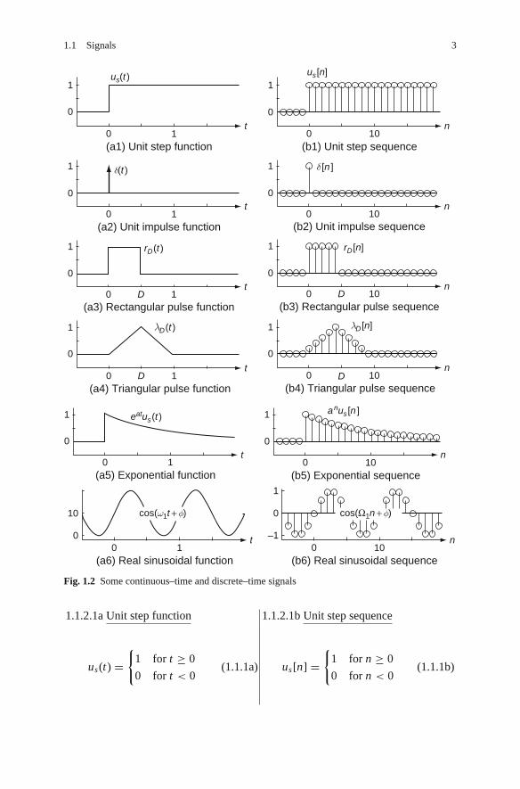
1.1 Signals 3
0
0(a1) Unit step function
us(t )
t
1
1
(a2) Unit impulse function
δ(t )
t0 1
0
1
(a3) Rectangular pulse function
rD(t )
t0 D 1
0
1
(a4) Triangular pulse function
λD(t )
t0 D 1
0
1
(a5) Exponential function
eatus(t )
t0 1
0
1
(b2) Unit impulse sequence
δ [n ]
n0 10
0
1
(b3) Rectangular pulse sequence
rD[n]
n0 D 10
0
1
(b1) Unit step sequence
us[n]
n0 10
0
1
(b4) Triangular pulse sequence
λD[n]
n0 D 10
0
1
(b5) Exponential sequence
anus[n ]
n0 10
0
1
(a6) Real sinusoidal function
cos(ω1t + φ)
t0 1
0
10
(b6) Real sinusoidal sequence
cos(Ω1n + φ)
n0 10
0
–1
1
Fig. 1.2 Some continuous–time and discrete–time signals
1.1.2.1a Unit step function 1.1.2.1b Unit step sequence
us(t) ={
1 for t ≥ 0
0 for t < 0(1.1.1a) us[n] =
{1 for n ≥ 0
0 for n < 0(1.1.1b)
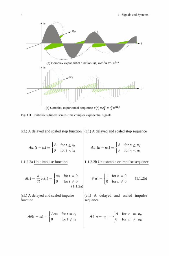
4 1 Signals and Systems
Im
Im
Re
Re
(a) Complex exponential function x (t ) = e
s1t = e
σ1t e
j ω1t
t
n
(b) Complex exponential sequence x (n) = z1n n= r1 e
j Ω1n
Fig. 1.3 Continuous–time/discrete–time complex exponential signals
(cf.) A delayed and scaled step function (cf.) A delayed and scaled step sequence
Aus(t − t0) ={
A for t ≥ t00 for t < t0
Aus[n − n0] ={
A for n ≥ n0
0 for n < n0
1.1.2.2a Unit impulse function 1.1.2.2b Unit sample or impulse sequence
δ(t) = d
dtus(t) =
{∞ for t = 0
0 for t �= 0(1.1.2a)
δ[n] ={
1 for n = 0
0 for n �= 0(1.1.2b)
(cf.) A delayed and scaled impulsefunction
(cf.) A delayed and scaled impulsesequence
Aδ(t − t0) ={
A∞ for t = t00 for t �= t0
A δ[n − n0] ={
A for n = n0
0 for n �= n0

1.1 Signals 5
(cf.) Relationship between δ(t) and us(t)
δ(t) = d
dtus(t) (1.1.3a)
us(t) =∫ t
−∞δ(τ )dτ (1.1.4a)
1.1.2.3a Rectangular pulse function
rD(t) = us(t) − us(t − D) (1.1.5a)
={
1 for 0 ≤ t < D (D : duration)
0 elsewhere
1.1.2.4a Unit triangular pulse function
λD(t) ={
1 − |t − D|/D for |t − D| ≤ D0 elsewhere
(1.1.6a)1.1.2.5a Real exponential function
x(t) = eat us(t) ={
eat for t ≥ 0
0 for t < 0(1.1.7a)
1.1.2.6a Real sinusoidal function
x(t) = cos(ω1t + φ) = Re{e j(ω1t+φ)}= 1
2
{e jφe jω1t + e− jφe− jω1t
}(1.1.8a)
1.1.2.7a Complex exponential function
x(t) = es1t =eσ1t e jω1t with s1 = σ1 + jω1
(1.1.9a)
Note that σ1 determines the changingrate or the time constant and ω1 theoscillation frequency.
1.1.2.8a Complex sinusoidal function
x(t) = e jω1t = cos(ω1t) + j sin(ω1t)(1.1.10a)
(cf) Relationship between δ[n] and us[n]
δ[n] = us[n] − us[n − 1] (1.1.3b)
us[n] =∑n
m=−∞ δ[m] (1.1.4b)
1.1.2.3b Rectangular pulse sequence
rD[n] = us[n] − us[n − D] (1.1.5b)
={
1 for 0 ≤ n < D (D : duration)
0 elsewhere
1.1.2.4b Unit triangular pulse sequence
λD[n] ={
1 − |n + 1 − D|/D for |n + 1 − D| ≤ D − 1
0 elsewhere
(1.1.6b)1.1.2.5b Real exponential sequence
x[n] = anus[n] ={
an for n ≥ 0
0 for n < 0(1.1.7b)
1.1.2.6b Real sinusoidal sequence
x[n] = cos(Ω1n + φ) = Re{e j(Ω1n+φ)
}= 1
2
{e jφe jΩ1n + e− jφe− jΩ1n
}(1.1.8b)
1.1.2.7b Complex exponential function
x[n] = zn1 = rn
1 e jΩ1n with z1 = r1e jΩ1
(1.1.9b)
Note that r1 determines the changingrate and Ω1 the oscillation frequency.
1.1.2.8b Complex sinusoidal sequence
x[n] = e jΩ1n = cos(Ω1n) + j sin(Ω1n)(1.1.10b)

6 1 Signals and Systems
1.1.3 Analog Frequency and Digital Frequency
A continuous-time signal x(t) is periodic with period P if P is generally the smallestpositive value such that x(t + P) = x(t). Let us consider a continuous-time periodicsignal described by
x(t) = e jω1t (1.1.11)
The analog or continuous-time (angular) frequency1 of this signal is ω1 [rad/s] andits period is
P = 2π
ω1[s] (1.1.12)
where
e jω1(t+P) = e jω1t ∀ t (∵ ω1 P = 2π ⇒ e jω1 P = 1) (1.1.13)
If we sample the signal x(t) = e jω1t periodically at t = nT , we get a discrete-time signal
x[n] = e jω1nT = e jΩ1n with Ω1 = ω1T (1.1.14)
Will this signal be periodic in n? You may well think that x[n] is also periodicfor any sampling interval T since it is obtained from the samples of a continuous-time periodic signal. However, the discrete-time signal x[n] is periodic only whenthe sampling interval T is the continuous-time period P multiplied by a rationalnumber, as can be seen from comparing Fig. 1.4(a) and (b). If we sample x(t) =e jω1t to get x[n] = e jω1nT = e jΩ1n with a sampling interval T = m P/N [s/sample]where the two integers m and N are relatively prime (coprime), i.e., they have nocommon divisor except 1, the discrete-time signal x[n] is also periodic with thedigital or discrete-time frequency
Ω1 = ω1T = ω1m P
N= m
N2π [rad/sample] (1.1.15)
The period of the discrete-time periodic signal x[n] is
N = 2mπ
Ω1[sample], (1.1.16)
where
e jΩ1(n+N ) = e jΩ1ne j2mπ = e jΩ1n ∀ n (1.1.17)
1 Note that we call the angular or radian frequency measured in [rad/s] just the frequency with-out the modifier ‘radian’ or ‘angular’ as long as it can not be confused with the ‘real’ frequencymeasured in [Hz].

1.1 Signals 7
1 2 3
1
00
0 1 2 3 4
0.5 1.5 2.5
(a) Sampling x (t ) = sin(3πt ) with sample period T = 0.25
(b) Sampling x (t ) = sin(3πt ) with sample period T = 1/π
3.5 4t
t
–1
1
0
–1
Fig. 1.4 Sampling a continuous–time periodic signal
This is the counterpart of Eq. (1.1.12) in the discrete-time case. There are severalobservations as summarized in the following remark:
Remark 1.1 Analog (Continuous-Time) Frequency and Digital (Discrete-Time)Frequency
(1) In order for a discrete-time signal to be periodic with period N (being aninteger), the digital frequency Ω1 must be π times a rational number.
(2) The period N of a discrete-time signal with digital frequency Ω1 is the mini-mum positive integer to be multiplied by Ω1 to make an integer times 2π like2mπ (m: an integer).
(3) In the case of a continuous-time periodic signal with analog frequency ω1, itcan be seen to oscillate with higher frequency as ω1 increases. In the case ofa discrete-time periodic signal with digital frequency Ω1, it is seen to oscillatefaster as Ω1 increases from 0 to π (see Fig. 1.5(a)–(d)). However, it is seento oscillate rather slower as Ω1 increases from π to 2π (see Fig. 1.5(d)–(h)).Particularly with Ω1 = 2π (Fig. 1.5(h)) or 2mπ , it is not distinguishable froma DC signal with Ω1 = 0. The discrete-time periodic signal is seen to oscillatefaster as Ω1 increases from 2π to 3π (Fig. 1.5(h) and (i)) and slower again asΩ1 increases from 3π to 4π .

8 1 Signals and Systems
1
0
–1
1
0
–1
1
0
–1
1
0
–1
1
0
–1
1
0
–1
1
0
–1
1
0
–1
1
0
–10 0.5
(a) cos(πnT), T = 0.25 (b) cos(2πnT ), T = 0.25 (c) cos(3πnT ), T = 0.25
(d) cos(4πnT ), T = 0.25 (e) cos(5πnT ), T = 0.25 (f) cos(6πnT), T = 0.25
(g) cos(7πnT ), T = 0.25 (h) cos(8πnT ), T = 0.25 (i) cos(9πnT ), T = 0.25
1 1.5 2
0 0.5 1 1.5 2
0 0.5 1 1.5 2 0 0.5 1 1.5 2 0 0.5 1 1.5 2
0 0.5 1 1.5 2 0 0.5 1 1.5 2
0 0.5 1 1.5 2 0 0.5 1 1.5 2
Fig. 1.5 Continuous–time/discrete–time periodic signals with increasing analog/digital frequency
This implies that the frequency characteristic of a discrete-time signal is peri-odic with period 2π in the digital frequency Ω. This is because e jΩ1n is alsoperiodic with period 2π in Ω1, i.e., e j(Ω1+2mπ )n = e jΩ1ne j2mnπ = e jΩ1n for anyinteger m.
(4) Note that if a discrete-time signal obtained from sampling a continuous-timeperiodic signal has the digital frequency higher than π [rad] (in its absolutevalue), it can be identical to a lower-frequency signal in discrete time. Such aphenomenon is called aliasing, which appears as the stroboscopic effect or thewagon-wheel effect that wagon wheels, helicopter rotors, or aircraft propellersin film seem to rotate more slowly than the true rotation, stand stationary, oreven rotate in the opposite direction from the true rotation (the reverse rotationeffect).[W-1]
1.1.4 Properties of the Unit Impulse Functionand Unit Sample Sequence
In Sect. 1.1.2, the unit impulse, also called the Dirac delta, function is defined byEq. (1.1.2a) as
δ(t) = d
dtus(t) =
{∞ for t = 0
0 for t �= 0(1.1.18)
1.1 Signals 9
Several useful properties of the unit impulse function are summarized in the follow-ing remark:
Remark 1.2a Properties of the Unit Impulse Function δ(t)
(1) The unit impulse function δ(t) has unity area around t = 0, which means
∫ +∞
−∞δ(τ )dτ =
∫ 0+
0−δ(τ )dτ = 1 (1.1.19)(
∵∫ 0+
−∞δ(τ )dτ −
∫ 0−
−∞δ(τ )dτ
(1.1.4a)= us(0+) − us(0−) = 1 − 0 = 1
)
(2) The unit impulse function δ(t) is symmetric about t = 0, which is described by
δ(t) = δ(−t) (1.1.20)
(3) The convolution of a time function x(t) and the unit impulse function δ(t) makesthe function itself:
x(t) ∗ δ(t)(A.17)=
definition of convolution integral
∫ +∞
−∞x(τ )δ(t − τ )dτ = x(t) (1.1.21)
⎛⎝∵ ∫ +∞
−∞ x(τ )δ(t − τ )dτδ(t−τ )�=0 for only τ=t= ∫ +∞
−∞ x(t)δ(t − τ )dτx(t) independent of τ= x(t)
∫ +∞−∞ δ(t − τ )dτ
t−τ→t ′= x(t)∫ t−∞
t+∞ δ(t ′)(−dt ′) = x(t)∫ t+∞
t−∞ δ(t ′)dt ′ = x(t)∫ +∞−∞ δ(τ )dτ
(1.1.19)= x(t)
⎞⎠
What about the convolution of a time function x(t) and a delayed unit impulsefunction δ(t − t1)? It becomes the delayed time function x(t − t1), that is,
x(t) ∗ δ(t − t1) =∫ +∞
−∞x(τ )δ(t − τ − t1)dτ = x(t − t1) (1.1.22)
What about the convolution of a delayed time function x(t − t2) and a delayedunit impulse function δ(t − t1)? It becomes another delayed time function x(t −t1 − t2), that is,
x(t − t2) ∗ δ(t − t1) =∫ +∞
−∞x(τ − t2)δ(t − τ − t1)dτ = x(t − t1 − t2) (1.1.23)
If x(t) ∗ y(t) = z(t), we have
x(t − t1) ∗ y(t − t2) = z(t − t1 − t2) (1.1.24)
However, with t replaced with t − t1 on both sides, it does not hold, i.e.,
x(t − t1) ∗ y(t − t1) �= z(t − t1), but x(t − t1)∗ y(t − t1) = z(t − 2t1)

10 1 Signals and Systems
(4) The unit impulse function δ(t) has the sampling or sifting property that
∫ +∞
−∞x(t)δ(t − t1)dt
δ(t−t1)�=0 for only t=t1= x(t1)∫ +∞
−∞δ(t − t1)dt
(1.1.19)= x(t1)
(1.1.25)
This property enables us to sample or sift the sample value of a continuous-timesignal x(t) at t = t1. It can also be used to model a discrete-time signal obtainedfrom sampling a continuous-time signal.
In Sect. 1.1.2, the unit-sample, also called the Kronecker delta, sequence isdefined by Eq. (1.1.2b) as
δ[n] ={
1 for n = 0
0 for n �= 0(1.1.26)
This is the discrete-time counterpart of the unit impulse function δ(t) and thus isalso called the discrete-time impulse. Several useful properties of the unit-samplesequence are summarized in the following remark:
Remark 1.2b Properties of the Unit-Sample Sequence δ[n]
(1) Like Eq. (1.1.20) for the unit impulse δ(t), the unit-sample sequence δ[n] is alsosymmetric about n = 0, which is described by
δ[n] = δ[−n] (1.1.27)
(2) Like Eq. (1.1.21) for the unit impulse δ(t), the convolution of a time sequencex[n] and the unit-sample sequence δ[n] makes the sequence itself:
x[n] ∗ δ[n]definition of convolution sum=
∑∞m=−∞ x[m]δ[n − m] =x[n] (1.1.28)
⎛⎜⎜⎜⎜⎜⎜⎝
∵∑∞
m=−∞ x[m]δ[n − m]δ[n−m]�=0 for only m=n= ∑∞
m=−∞ x[n]δ[n − m]
x[n] independent of m= x[n]∑∞
m=−∞ δ[n − m]
δ[n−m]�=0 for only m=n= x[n]δ[n − n](1.1.26)= x[n]
⎞⎟⎟⎟⎟⎟⎟⎠

1.1 Signals 11
(3) Like Eqs. (1.1.22) and (1.1.23) for the unit impulse δ(t), the convolution of atime sequence x[n] and a delayed unit-sample sequence δ[n − n1] makes thedelayed sequence x[n − n1]:
x[n] ∗ δ[n − n1] =∑∞
m=−∞ x[m]δ[n − m − n1] =x[n − n1] (1.1.29)
x[n − n2] ∗ δ[n − n1] =∑∞
m=−∞ x[m − n2]δ[n − m − n1] =x[n − n1 − n2]
(1.1.30)
Also like Eq. (1.1.24), we have
x[n] ∗ y[n] = z[n] ⇒ x[n − n1] ∗ y[n − n2] = z[n − n1 − n2] (1.1.31)
(4) Like (1.1.25), the unit-sample sequence δ[n] has the sampling or sifting prop-erty that
∑∞n=−∞ x[n]δ[n − n1] =
∑∞n=−∞ x[n1]δ[n − n1] =x[n1] (1.1.32)
1.1.5 Several Models for the Unit Impulse Function
As depicted in Fig. 1.6(a)–(d), the unit impulse function can be modeled by the limitof various functions as follows:
− δ(t) = limD→0+
1
D
sin(π t/D)
π t/D= lim
D→0+
1
Dsinc(t/D)
π/D→w= limw→∞
w
π
sin(wt)
wt(1.1.33a)
− δ(t) = limD→0+
1
DrD
(t + D
2
)(1.1.33b)
− δ(t) = limD→0+
1
DλD (t + D) (1.1.33c)
− δ(t) = limD→0+
1
2De−|t |/D (1.1.33d)
Note that scaling up/down the impulse function horizontally is equivalent to scalingit up/down vertically, that is,
δ(at) = 1
|a|δ(t) (1.1.34)
It is easy to show this fact with any one of Eqs. (1.1.33a–d). Especially forEq. (1.1.33a), that is the sinc function model of δ(t), we can prove the validity ofEq. (1.1.34) as follows:

12 1 Signals and Systems
8 D = 0.125
D = 0.250
D = 0.500D = 1.000
D = 0.125
D = 0.250
D = 0.500D = 1.000
D = 0.125
D = 0.250
D = 0.500D = 1.000
D = 0.0625
D = 0.125
D = 0.250D = 0.500
6
4
2
0
8
6
4
2
0
–1.5 –1 –0.5 0 0.5 1 1.5
8
6
4
2
0
–1.5 –1 –0.5 0 0.5 1 1.5
8
6
4
2
0
–1.5 –1 –0.5 0 0.5 1 1.5
–1.5 –1 –0.5 0 0.5 1 1.5
D 2(b) rD
(t + )1 D
D(c) λD (t + D )1
(a)1 sin (πt /D)
πt /DD1
sinc ( )=D
tD
e– t / D
2D(d) 1
Fig. 1.6 Various models of the unit impulse function δ(t)
δ(at)(1.1.33a)= lim
D→0+
1
D
sin(πat/D)
πat/D= lim
D/|a|→0+
1
|a|(D/|a|)sin(π t/(D/a))
π t/(D/a)D/|a|→D′
= 1
|a| limD′→0+
1
D′sin(π t/D′)
π t/D′(1.1.33a)= 1
|a|δ(t)
On the other hand, the unit-sample or impulse sequence δ[n] can be written as
δ[n] = sin(πn)
πn= sinc(n) (1.1.35)
where the sinc function is defined as
sinc(x) = sin(πx)
πx(1.1.36)
1.2 Systems
A system is a plant or a process that produces a response called an output inresponse to an excitation called an input. If a system’s input and output signalsare scalars, the system is called a single-input single-output (SISO) system. If asystem’s input and output signals are vectors, the system is called a multiple-input

1.2 Systems 13
the input the output
(a) A continuous−time system (b) A discrete−time system
G Gy (t ) = G {x (t )}x (t )the input the output
y [n] = G {x [n ] }x [n]
Fig. 1.7 A description of continuous–time and discrete–time systems
multiple-output (MIMO) system. A single-input multiple-output (SIMO) system anda multiple-input single-output (MISO) system can also be defined in a similar way.For example, a spring-damper-mass system is a mechanical system whose outputto an input force is the displacement and velocity of the mass. Another exampleis an electric circuit whose inputs are voltage/current sources and whose outputsare voltages/currents/charges in the circuit. A mathematical operation or a com-puter program transforming input argument(s) (together with the initial conditions)into output argument(s) as a model of a plant or a process may also be calleda system.
A system is called a continuous-time/discrete-time system if its input and outputare both continuous-time/discrete-time signals. Continuous-time/discrete-time sys-tems with the input and output are often described by the following equations andthe block diagrams depicted in Fig. 1.7(a)/(b).
Continuous-time system
x(t)G{}→ y(t); y(t) = G{x(t)}
Discrete-time system
x[n]G{}→ y[n]; y[n] = G{x[n]}
1.2.1 Linear System and Superposition Principle
A system is said to be linear if the superposition principle holds in the sense that itsatisfies the following properties:
- Additivity: The output of the system excited by more than one independentinput is the algebraic sum of its outputs to each of the inputsapplied individually.
- Homogeneity: The output of the system to a single independent input isproportional to the input.
This superposition principle can be expressed as follows:
If the output to xi (t) is yi (t) = G{xi (t)},the output to
∑i
ai xi (t) is∑
iai G{xi (t)},
that is,
If the output to xi [n] is yi [n] =G{xi [n]}, the output to
∑i
ai xi [n] is∑i
ai G {xi [n]}, that is,
14 1 Signals and Systems
G
{∑i
ai xi (t)
}=∑
i
ai G{xi (t)}
=∑
i
ai yi (1.2.1a)
(Ex) A continuous-time linear system
y(t) = 2x(t)
(Ex) A continuous-time nonlinear system
y(t) = x(t) + 1
G
{∑i
ai xi [n]
}=∑
i
ai G{xi [n]}
=∑
i
ai yi [n] (1.2.1b)
(Ex) A discrete-time linear system
y[n] = 2x[n]
(Ex) A discrete-time nonlinear system
y[n] = x2[n]
Remark 1.3 Linearity and Incremental Linearity
(1) Linear systems possess a property that zero input yields zero output.(2) Suppose we have a system which is essentially linear and contains some
memory (energy storage) elements. If the system has nonzero initial condi-tion, it is not linear any longer, but just incrementally linear, since it violatesthe zero-input/zero-output condition and responds linearly to changes in theinput. However, if the initial condition is regarded as a kind of input usuallyrepresented by impulse functions, then the system may be considered to belinear.
1.2.2 Time/Shift-Invariant System
A system is said to be time/shift-invariant if a delay/shift in the input causesonly the same amount of delay/shift in the output without causing any change ofthe charactersitic (shape) of the output. Time/shift-invariance can be expressed asfollows:
If the output to x(t) is y(t), the output tox(t − t1) is y(t − t1), i.e.,
G {x(t − t1)} = y(t − t1) (1.2.2a)
(Ex) A continuous-time time-invariantsystem
y(t) = sin(x(t))
If the output to x[n] is y[n], the outputto x[n − n1] is y[n − n1], i.e.,
G {x[n − n1]} = y[n − n1] (1.2.2b)
(Ex) A discrete-time time-invariantsystem
y[n] = 1
3(x[n − 1] + x[n] + x[n + 1])

1.2 Systems 15
(Ex) A continuous-time time-varyingsystem
y′(t) = (sin(t) − 1)y(t) + x(t)
(Ex) A discrete-time time-varyingsystem
y[n] = 1
ny[n − 1] + x[n]
1.2.3 Input-Output Relationship of LinearTime-Invariant (LTI) System
Let us consider the output of a continuous-time linear time-invariant (LTI) systemG to an input x(t). As depicted in Fig. 1.8, a continuous-time signal x(t) of anyarbitrary shape can be approximated by a linear combination of many scaled andshifted rectangular pulses as
x(t) =∑∞
m=−∞ x(mT )1
TrT
(t + T
2− mT
)T
T →dτ,mT →τ→(1.1.33b)
x(t) = limT →0
x(t) =∫ ∞
−∞x(τ )δ(t − τ )dτ = x(t) ∗δ(t) (1.2.3)
Based on the linearity and time-invariance of the system, we can apply the superpo-sition principle to write the output y(t) to x(t) and its limit as T → 0:
y(t) = G{x(t)} =∑∞
m=−∞ x(mT )gT (t − mT )T
y(t) = G{x(t)} =∫ ∞
−∞x(τ )g(t − τ )dτ = x(t)∗g(t) (1.2.4)
Here we have used the fact that the limit of the unit-area rectangular pulse responseas T → 0 is the impulse response g(t), which is the output of a system to a unitimpulse input:
(a) Rectangular pulse
1
0 0 0
1rT
(t )
Tt t
(b) Rectangular pulse shifted by –T/2
(c) A continuous–time signal approximated by a linear combination of scaled/shifted rectangular pulses
–T/2 T/2–2T
x (t )
x (t ) x (0)x (–T ) x (T )
x (2T )x (3T )
x (–2T )
^
3T2TT–T
+ T2 )rT
(t
Fig. 1.8 The approximation of a continuous-time signal using rectangular pulses

16 1 Signals and Systems
gT (t) = G
{1
TrT
(t + T
2
)}: the response of the LTI system to a unit-area
rectangular pulse input
T →0→ limT →0
gT (t) = limT →0
G
{1
TrT
(t + T
2
)}
= G
{limT →0
1
TrT
(t + T
2
)}(1.1.33b)= G{δ(t)} = g(t) (1.2.5)
To summarize, we have an important and fundamental input-output relationship(1.2.4) of a continuous-time LTI system (described by a convolution integral inthe time domain) and its Laplace transform (described by a multiplication in thes-domain)
y(t) = x(t)∗ g(t)Laplace transform→
Table B.7(4)Y (s) = X (s)G(s) (1.2.6)
where the convolution integral, also called the continuous-time convolution, isdefined as
x(t)∗ g(t) =∫ ∞
−∞x(τ )g(t − τ )dτ =
∫ ∞
−∞g(τ )x(t − τ )dτ = g(t)∗ x(t) (1.2.7)
(cf.) This implies that the output y(t) of an LTI system to an input can be expressedas the convolution (integral) of the input x(t) and the impulse response g(t).
Now we consider the output of a discrete-time linear time-invariant (LTI) systemG to an input x[n]. We use Eq. (1.1.28) to express the discrete-time signal x[n] ofany arbitrary shape as
x[n](1.1.28)= x[n]∗ δ[n]
definition of convolution sum=∑∞
m=−∞ x[m]δ[n − m] (1.2.8)
Based on the linearity and time-invariance of the system, we can apply the superpo-sition principle to write the output to x[n]:
y[n] = G{x[n]} (1.2.8)= G{∑∞
m=−∞ x[m]δ[n − m]}
linearity=∑∞
m=−∞ x[m]G{δ[n − m]}
time−invariance=∑∞
m=−∞ x[m]g[n − m] = x[n]∗ g[n] (1.2.9)
Here we have used the definition of the impulse response or unit-sample responseof a discrete-time system together with the linearity and time-invariance of thesystem as
1.2 Systems 17
G{δ[n]} = g[n]time−invariance→ G{δ[n − m]} = g[n − m]
G{x[m]δ[n − m]} linearity= x[m]G{δ[n − m]} time−invariance= x[m]g[n − m]
To summarize, we have an important and fundamental input-output relationship(1.2.9) of a discrete-time LTI system (described by a convolution sum in the timedomain) and its z-transform (described by a multiplication in the z-domain)
y[n] = x[n]∗ g[n]z−transform→Table B.7(4)
Y [z] = X [z]G[z] (1.2.10)
where the convolution sum, also called the discrete-time convolution, is defined as
x[n]∗ g[n] =∑∞
m=−∞ x[m]g[n − m] =∑∞
m=−∞ g[m]x[n − m] = g[n]∗ x[n]
(1.2.11)
(cf.) If you do not know about the z-transform, just think of it as the discrete-timecounterpart of the Laplace transform and skip the part involved with it. Youwill meet with the z-transform in Chap. 4.
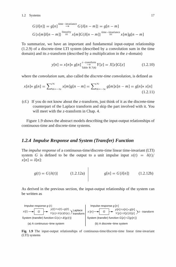
Figure 1.9 shows the abstract models describing the input-output relationships ofcontinuous-time and discrete-time systems.
1.2.4 Impulse Response and System (Transfer) Function
The impulse response of a continuous-time/discrete-time linear time-invariant (LTI)system G is defined to be the output to a unit impulse input x(t) = δ(t)/x[n] = δ[n]:
g(t) = G{δ(t)} (1.2.12a) g[n] = G{δ[n]} (1.2.12b)
As derived in the previous section, the input-output relationship of the system canbe written as
Impulse response g (t )
System (transfer) function G (s )=L{g (t )}
(a) A continuous−time system
Laplacetransform
x (t )y (t )=x (t ) * g (t ) y [n ]=x [n ] * g [n ]
Y [z ]=X [z ] G [z ]Y (s )=X (s )G (s )G
Impulse response g [n ]
System (transfer) function G [z ]=Z{g [n ] }
(b) A discrete−time system
z - transformx [n ] G
Fig. 1.9 The input-output relationships of continuous-time/discrete-time linear time-invariant(LTI) systems

18 1 Signals and Systems
y(t)(1.2.7)= x(t)∗ g(t)
L↔ Y (s)(1.2.6)= X (s)G(s) y[n]
(1.2.11)= x[n]∗ g[n]Z↔ Y [z]
(1.2.10)= X [z]G[z]
where x(t)/x[n], y(t)/y[n], and g(t)/g[n] are the input, output, and impulseresponse of the system. Here, the transform of the impulse response, G(s)/G[z],is called the system or transfer function of the system. We can also rewrite theseequations as
G(s) = Y (s)
X (s)= L{y(t)}
L{x(t)} = L{g(t)}(1.2.13a)
G[z] = Y [z]
X [z]= Z{y[n]}
Z{x[n]} = Z{g[n]}(1.2.13b)
This implies another definition or interpretation of the system or transfer functionas the ratio of the transformed output to the transformed input of a system with noinitial condition.
1.2.5 Step Response, Pulse Response, and Impulse Response
Let us consider a continuous-time LTI system with the impulse response and transferfunction given by
g(t) = e−at us(t) and G(s)(1.2.13a)= L{g(t)} = L{e−at us(t)} Table A.1(5)= 1
s + a,
(1.2.14)
respectively. We can use Eq. (1.2.6) to get the step response, that is the output to the
unit step input x(t) = us(t) with X (s)Table A.1(3)= 1/s, as
Ys(s) = G(s)X (s) = 1
s + a
1
s= 1
a
(1
s− 1
s + a
);
ys(t) = L−1{Ys(s)} Table A.1(3),(5)= 1
a(1 − e−at )us(t) (1.2.15)
Now, let a unity-area rectangular pulse input of duration (pulsewidth) T andheight 1/T
x(t) = 1
TrT (t) = 1
T(us(t) − us(t − T )); X (s) = L{x(t)} = 1
TL{us(t) − us(t − T )}
Table A.1(3), A.2(2)= 1
T
(1
s− e−T s 1
s
)(1.2.16)
be applied to the system. Then the output gT (t), called the pulse response, isobtained as

1.2 Systems 19
Impulse
Impulseresponse
00.0
1
T = 0.5T = 1.00
T rT
(t )
gT (t )
Rectangular pulse
Pulse response
1.0 2.0 3.0 4.0t
δ (t )
g (t )
0 ←T
T = 0.125
T = 0.25
Fig. 1.10 The pulse response and the impulse response
YT (s) = G(s)X (s) = 1
T
(1
s(s + a)− e−T s 1
s(s + a)
)
= 1
aT
(1
s− 1
s + a− e−T s
(1
s− 1
s + a
)); gT (t) = L−1{YT (s)}
Table A.1(3),(5),A.2(2)= 1
aT
((1 − e−at )us(t) − (1 − e−a(t−T ))us(t − T )
)(1.2.17)
If we let T → 0 so that the rectangular pulse input becomes an impulse δ(t) (ofinstantaneous duration and infinite height), how can the output be expressed? Tak-ing the limit of the output equation (1.2.17) with T → 0, we can get the impulseresponse g(t) (see Fig. 1.10):
gT (t)T →0→ 1
aT
((1 − e−at )us(t) − (1 − e−a(t−T ))us(t)
) = 1
aT(eaT − 1)e−at us(t)
(D.25)∼=aT →0
1
aT(1 + aT − 1)e−at us(t) = e−at us(t)
(1.2.14)≡ g(t) (1.2.18)
This implies that as the input gets close to an impulse, the output becomes close tothe impulse response, which is quite natural for any linear time-invariant system.
On the other hand, Fig. 1.11 shows the validity of Eq. (1.2.4) insisting that thelinear combination of scaled/shifted pulse responses gets closer to the true output asT → 0.
1.2.6 Sinusoidal Steady-State Responseand Frequency Response
Let us consider the sinusoidal steady-state response, which is defined to be the ever-lasting output of a continuous-time system with system function G(s) to a sinusoidalinput, say, x(t) = A cos(ωt + φ). The expression for the sinusoidal steady-state

20 1 Signals and Systems
: x(t ): x(t )
: x(t )
1
0.5
0.5 1 1.5 2
0.4
0.2
00 1 2 3 4
0.4
0.2
00 1 2 3 4
0
1
0
1
0.5
0.5 1 1.5 20
0
^
: x(t )^:y (t ) =
2
3
1
2
3
4
5
1
2
3
5
1 2 3
43
21
T
T
+ + +...
:y (t ) = 1 2 3+ +
: y (t )
: y (t )
(a1) The input x (t ) and its approximation x (t ) with T = 0.5^
(a2) The input x (t ) and its approximation x (t ) with T = 0.25^ (b2) The outputs to x (t ) and x (t )^
^
(b1) The outputs to x (t ) and x (t )^
^
Fig. 1.11 The input–output relationship of a linear time–invariant (LTI) system – convolution
response can be obtained from the time-domain input-output relationship (1.2.4).That is, noting that the sinusoidal input can be written as the sum of two complexconjugate exponential functions
x(t) = A cos (ωt + φ)(D.21)= A
2(e j(ωt+φ) + e− j(ωt+φ)) = A
2(x1(t) + x2(t)), (1.2.19)
we substitute x1(t) = e j(ωt+φ) for x(t) into Eq. (1.2.4) to obtain a partial steady-stateresponse as
y1(t) = G{x1(t)} (1.2.4)=∫ ∞
−∞x1(τ )g(t − τ )dτ =
∫ ∞
−∞e j(ωτ+φ)g(t − τ )dτ
= e j(ωt+φ)∫ ∞
−∞e− jω(t−τ )g(t − τ )dτ = e j(ωt+φ)
∫ ∞
−∞e− jωt g(t)dt
= e j(ωt+φ)G( jω) (1.2.20)
with
G( jω) =∫ ∞
−∞e− jωt g(t)dt
g(t)=0 for t<0=causal system
∫ ∞
0g(t)e− jωt dt
(A.1)= G(s)|s= jω (1.2.21)
Here we have used the definition (A.1) of the Laplace transform under the assump-tion that the impulse response g(t) is zero ∀t < 0 so that the system is causal (seeSect. 1.2.9). In fact, every physical system satisfies the assumption of causality thatits output does not precede the input. Here, G( jω) obtained by substituting s = jω(ω: the analog frequency of the input signal) into the system function G(s) is calledthe frequency response.

1.2 Systems 21
The total sinusoidal steady-state response to the sinusoidal input (1.2.19) can beexpressed as the sum of two complex conjugate terms:
y(t) = A
2
(y1(t) + y2(t)
)= A
2
{e j(ωt+φ)G( jω) + e− j(ωt+φ)G(− jω)
}
= A
2
{e j(ωt+φ)|G( jω)|e jθ(ω) + e− j(ωt+φ)|G(− jω)|e− jθ(ω)
= A
2|G( jω)|
{e j(ωt+φ+θ(ω)) + e− j(ωt+φ+θ(ω))
}
(D.21)= A|G( jω)| cos(ωt + φ + θ (ω)) (1.2.22)
where |G( jω)| and θ (ω) = ∠G( jω) are the magnitude and phase of the frequencyresponse G( jω), respectively. Comparing this steady-state response with the sinu-soidal input (1.2.19), we see that its amplitude is |G( jω)| times the amplitude A ofthe input and its phase is θ (ω) plus the phase φ of the input at the frequency ω ofthe input signal.
(cf.) The system function G(s) (Eq. (1.2.13a)) and frequency response G( jω)(Eq. (1.2.21)) of a system are the Laplace transform and Fourier transformof the impulse response g(t) of the system, respectively.
Likewise, the sinusoidal steady-state response of a discrete-time system to asinusoidal input, say, x[n] = A cos(Ωn + φ) turns out to be
y[n] = A|G[e jΩ]| cos(Ωn + φ + θ (Ω)) (1.2.23)
where
G[e jΩ] =∑∞
n=−∞ g[n]e− jΩn g[n]=0 for n<0=causal system
∑∞n=0
g[n]e− jΩn Remark 4.5= G[z]|z=e jΩ
(1.2.24)Here we have used the definition (4.1) of the z-transform. Note that G[e jΩ] obtainedby substituting z = e jΩ (Ω: the digital frequency of the input signal) into the systemfunction G[z] is called the frequency response.
Remark 1.4 Frequency Response and Sinusoidal Steady-State Response
(1) The frequency response G( jω) of a continuous-time system is obtained by sub-stituting s = jω (ω: the analog frequency of the input signal) into the systemfunction G(s). Likewise, the frequency response G[e jΩ] of a discrete-time sys-tem is obtained by substituting z = e jΩ (Ω: the digital frequency of the inputsignal) into the system function G[z].

22 1 Signals and Systems
(2) The steady-state response of a system to a sinusoidal input is also a sinusoidalsignal of the same frequency. Its amplitude is the amplitude of the input timesthe magnitude of the frequency response at the frequency of the input. Itsphase is the phase of the input plus the phase of the frequency response at thefrequency of the input (see Fig. 1.12).
Input x (t ) = Output y (t ) =A⎪G ( j ω) ⎪cos(ωt + φ + θ)
: Magnitude of the frequency response: Phase of the frequency response
(a) A continuous-time system
A cos(ωt + φ)
G ( j ω)θ( ω) = ∠G ( j ω)
G (s ) G [z ]Input x [n ] = Output y [n ] =
A⎪G( e j Ω) ⎪cos(Ωn + φ + θ )
(b) A discrete-time system
A cos(Ωn + φ)
G [e j Ω ] : Magnitude of the frequency response
θ( Ω) = ∠G [e j Ω ] : Phase of the frequency response
Fig. 1.12 The sinusoidal steady–state response of continuous-time/discrete-time linear time-invariant systems
1.2.7 Continuous/Discrete-Time Convolution
In Sect. 1.2.3, the output of an LTI system was found to be the convolution of theinput and the impulse response. In this section, we take a look at the process ofcomputing the convolution to comprehend its physical meaning and to be able toprogram the convolution process.
The continuous-time/discrete-time convolution y(t)/y[n] of two functions/sequences x(τ )/x[m] and g(τ )/g[m] can be obtained by time-reversing one of them,say, g(τ )/g[m] and time-shifting (sliding) it by t/n to g(t−τ )/g[n−m], multiplyingit with the other, say, x(τ )/x[m], and then integrating/summing the multiplication,say, x(τ )g(t − τ )/x[m]g[n − m]. Let us take a look at an example.
Example 1.1 Continuous-Time/Discrete-Time Convolution of Two RectangularPulses
(a) Continuous-Time Convolution (Integral) of Two Rectangular Pulse FunctionsrD1 (t) and rD2 (t) Referring to Fig. 1.13(a1–a8), you can realize that theconvolution of the two rectangular pulse functions rD1 (t) (of duration D1) andrD2 (t) (of duration D2 < D1) is
rD1(t)∗rD2 (t) =
⎧⎪⎪⎪⎨⎪⎪⎪⎩
t for 0 ≤ t < D2
D2 for D2 ≤ t < D1
−t + D for D1 ≤ t < D = D1 + D2
0 elsewhere
(E1.1.1a)
The procedure of computing this convolution is as follows:
- (a1) and (a2) show rD1 (τ ) and rD2 (τ ), respectively.- (a3) shows the time-reversed version of rD2 (τ ), that is rD2 (−τ ). Since there is
no overlap between rD1 (τ ) and rD2 (−τ ), the value of the convolution rD1 (t)∗rD2 (t) at t = 0 is zero.

1.2 Systems 23
(a1)
(a2)
(a3)
(a4)
(a5)
(a6)
(a7)
(a8)D2
D2
–D2
D2
D1
D2
D1
D1
0
0
0
0
0
0
0
0
D1
D
D = D1 + D2
r D1(τ) * rD2
(τ)
r D2(D1 – τ)
r D2(D1 + D2 – τ)
r D2(D2 – τ)
r D2(– τ)
r D2( τ)
r D1( τ)
t
D1 + D2
D1 – D2
τ (b1)
(b2)
(b3)
(b4)
(b5)
(b6)
(b7)
(b8)0
0
0
0
0
0
D = D1 + D2 – 1r D1
[n] * rD2[n]
D2 – 1
D1 – 1
D1 – 1
D2 – 1
–(D2 – 1)
0
0 1 2
D2 – 1
(D1 – 1)Ts
D1 – 1 D–1
D2
D1 + D2 – 2
r D2[D1 + D2 – 2 – m]
r D2[ D1 – 1 – m]
r D2[ D2 – 1 – m]
r D2[– m]
r D2[m]
r D1[m]
m
m
m
m
m
m
m
n
D1 – D2
Ts
τ[sec]
τ
τ
τ
τ
τ
τ
D1 – 1
Fig. 1.13 Continuous–time/discrete–time convolution of two rectangular pulses
- (a4) shows the D2-delayed version of rD2 (−τ ), that is rD2 (D2 − τ ). Sincethis overlaps with rD1 (τ ) for 0 ≤ τ < D2 and the multiplication of them is 1over the overlapping interval, the integration (area) is D2, which will be thevalue of the convolution at t = D2. In the meantime (from t = 0 to D2), itgradually increases from t = 0 to D2 in proportion to the lag time t .
- As can be seen from (a4)–(a6), the length of the overlapping interval betweenrD2 (t −τ ) and rD1 (τ ) and the integration of the multiplication is kept constantas D2 till rD2 (t − τ ) is slided by D1 to touch the right end of rD1 (τ ). Thus thevalue of the convolution is D2 all over D2 ≤ t < D1.

24 1 Signals and Systems
- While the sliding rD2 (t − τ ) passes by the right end of rD1 (τ ), the length ofthe overlapping interval with rD1 (τ ) and the integration of the multiplicationdecreases gradually from D2 to 0 till it passes through the right end of rD1 (τ )at t = D1 + D2 as shown in (a7).
- After the left end of rD2 (t − τ ) passes by the right end of rD1 (τ ) at t =D1 + D2, there is no overlap and thus the value of the convolution is zero allover t ≥ D1 + D2.
- The convolution obtained above is plotted against the time lag t in (a8).
(b) Discrete-Time Convolution (Sum) of Two Rectangular Pulse Sequences rD1 [n]and rD2 [n] Referring to Fig. 1.13(b1–b8), you can realize that the convolutionof the two rectangular pulse sequences rD1 [n] (of duration D1) and rD2 [n] (ofduration D2 < D1) is as follows:
rD1[n]∗rD2 [n] =
⎧⎪⎪⎪⎨⎪⎪⎪⎩
n + 1 for 0 ≤ n < D2
D2 for D2 ≤ n < D1
−n + D for D1 ≤ n < D = D1 + D2 − 1
0 elsewhere
(E1.1.1b)
The procedure of computing this discrete-time convolution is similar to thattaken to get the continuous-time convolution in (a). The difference is as follows:
- The value of rD1 [n] ∗ rD2 [n] is not zero at n = 0 while that of rD1 (t) ∗ rD2 (t)is zero at t = 0.
- The duration of rD1 [n] ∗ rD2 [n] is from n = 0 to D1 + D2 − 2 while that ofrD1 (t) ∗ rD2 (t) is from t = 0 to D1 + D2.
(cf.) You had better try to understand the convolution process rather graphicallythan computationally.
(cf.) Visit the web site <http://www.jhu.edu/∼signals/> to appreciate the joy ofconvolution.
Remark 1.5 Continuous-Time/Discrete-Time Convolution of Two RectangularPulses
(1) If the lengths of the two rectangular pulses are D1 and D2 (with D1 > D2),respectively, the continuous-time and discrete-time convolutions have the dura-tion of D1 + D2 and D1 + D2 − 1, respectively and commonly the heightof D2.
(2) If the lengths of the two rectangular pulses are commonly D, the continuous-time and discrete-time convolutions are triangular pulses whose durations are2D and 2D − 1, respectively and whose heights are commonly D:
rD(t)∗rD(t) = DλD(t) (1.2.25a)
rD[n]∗rD[n] = DλD[n] (1.2.25b)
1.2 Systems 25
3210
0 2 4 6T t [sec]
0 2 4 6T t [sec]
0 2 4 6T t [sec]
(a1) x (t )
x(t )
g (t )
(a2) g (t )
(a3) y (t ) = x (t )*g(t )
y1TλT (t−T )
y0TλT (t ) y2TλT (t − 2T )
–1
3 6
42
0
0 5 10
2
2(b1) xb[n ] (c1) xc[n ]
(c2) gc[n ]
gc[n ]
gb[n ]
(b2) gb[n ]
(b3) yb[n ] = xb[n ] *gb[n ] (c3) yc[n ] = xc[n ] *gc[n ]
4 6
10
0
–1
3210
–1
3210
–1
n
32
2 4 6
10
0
–1
n
32
2 4 6
10
0
–1
n
x3
x2Ts
x0
y0
y1 y2 y3
y4
y5
g0 g1 g2
x1 xb[n ]xc[n ]
n
6
42
0
0 5 10 n
6
42
0
0 5 10 n
Ts
Fig. 1.14 Approximation of a continuous–time convolution by a discrete–time convolution
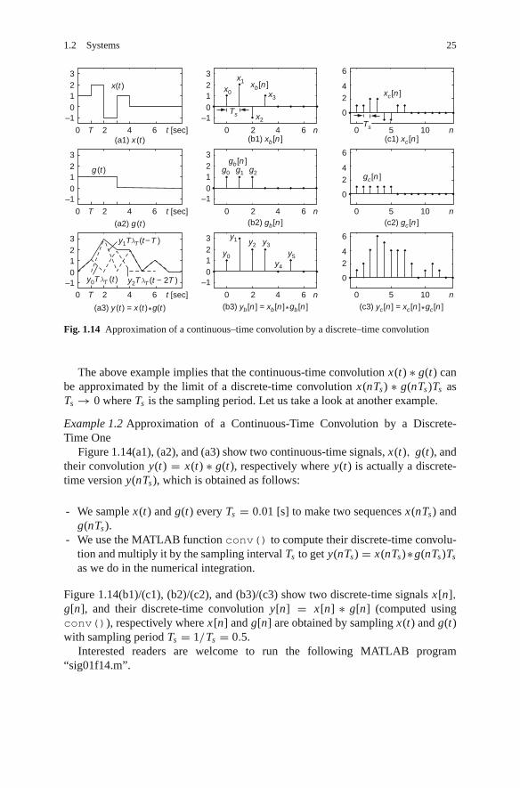
The above example implies that the continuous-time convolution x(t) ∗ g(t) canbe approximated by the limit of a discrete-time convolution x(nTs) ∗ g(nTs)Ts asTs → 0 where Ts is the sampling period. Let us take a look at another example.
Example 1.2 Approximation of a Continuous-Time Convolution by a Discrete-Time One
Figure 1.14(a1), (a2), and (a3) show two continuous-time signals, x(t), g(t), andtheir convolution y(t) = x(t) ∗ g(t), respectively where y(t) is actually a discrete-time version y(nTs), which is obtained as follows:
- We sample x(t) and g(t) every Ts = 0.01 [s] to make two sequences x(nTs) andg(nTs).
- We use the MATLAB function conv() to compute their discrete-time convolu-tion and multiply it by the sampling interval Ts to get y(nTs) = x(nTs)∗g(nTs)Ts
as we do in the numerical integration.
Figure 1.14(b1)/(c1), (b2)/(c2), and (b3)/(c3) show two discrete-time signals x[n],g[n], and their discrete-time convolution y[n] = x[n] ∗ g[n] (computed usingconv()), respectively where x[n] and g[n] are obtained by sampling x(t) and g(t)with sampling period Ts = 1/Ts = 0.5.
Interested readers are welcome to run the following MATLAB program“sig01f14.m”.

26 1 Signals and Systems
%sig01f14.m: Fig.1.14clear, clfx=[1 2 -1 1]; g=[1 1 1];t0 x=0;t0 g=0; %t0 x=1; t0 g=-2; % the initial time indices of x and g% Continuous-Time ConvolutionT=1; Ts=0.01; dt=Ts; M=T/Ts; %Interval T, Sampling period Ts, and # of Ts per Txt= ones(M,1)*x; xt=xt(:).’; Nxt=length(xt);gt= ones(M,1)*g; gt=gt(:).’; Ngt=length(gt);yt= conv(xt,gt)*Ts; Nyt=length(yt); % the length of convolution Nxt+Ngt-1NytM=Nyt+M; % plotting interval extended by one interval Tt0 y=t0 x+t0 g; tt= min([t0 x t0 g t0 y])+[0:NytM-1]*Ts;xt = [zeros(1,fix((t0 x-tt(1))/Ts)) xt]; xt =[xt zeros(1,NytM-length(xt ))];gt = [zeros(1,fix((t0 g-tt(1))/Ts)) gt]; gt =[gt zeros(1,NytM-length(gt ))];yt = [zeros(1,fix((t0 y-tt(1))/Ts)) yt]; yt = [yt zeros(1,NytM-length(yt ))];ymax= max([xt gt yt])+0.5; ymin= min([xt gt yt])-0.5;subplot(331), plot(tt,xt ), axis([tt([1 end]) ymin ymax])subplot(334), plot(tt,gt ), axis([tt([1 end]) ymin ymax])subplot(337), plot(tt,yt ), axis([tt([1 end]) ymin ymax])% Discrete-Time ConvolutionTs=1; n0 x = t0 x/Ts; n0 g = t0 g/Ts;xn=xt(1:Ts/dt:4*M), gn=gt(1:Ts/dt:3*M)Nx=length(xn); Ng=length(gn); % the length of convolution Nx+Ng-1yn=conv(xn,gn); Ny=length(yn);xn extended=[zeros(1,Ng-1) xn]; gn reversed= fliplr(gn);gr extended= [gn reversed zeros(1,Ny-Ng)];for n=1:Ny % Instead of conv(), we slide g[-n], multiply x[n], and take sum.
yn1(n)=xn extended*gr extended.’;gr extended= [0 gr extended(1:Ny-1)];
endNy1=Ny+3; % plotting interval extended by two samplesn0 y=n0 x+n0 g; nn= min([n0 x n0 g n0 y])+[-1:Ny1-2];xn = [zeros(1,n0 x-nn(1)) xn]; xn = [xn zeros(1,Ny1-length(xn ))];gn = [zeros(1,n0 g-nn(1)) gn]; gn = [gn zeros(1,Ny1-length(gn ))];yn = [zeros(1,n0 y-nn(1)) yn]; yn = [yn zeros(1,Ny1-length(yn ))];ymax= max([xn gn yn])+0.5; ymin= min([xn gn yn])-0.5;subplot(332), stem(nn,xn ,’.’), axis([nn([1 end]) ymin ymax])subplot(335), stem(nn,gn ,’.’), axis([nn([1 end]) ymin ymax])subplot(338), stem(nn,yn ,’.’), axis([nn([1 end]) ymin ymax])
The systems, called tapped delay lines, to be discussed in the following exampleare essentially continuous-time systems. However, they behave like discrete-timesystems in terms of the input-output relationship and thus are expected to be a linkbetween continuous-time systems and discrete-time ones.
Example 1.3 Tapped Delay Lines
(a) Tapped Delay LinesConsider the continuous-time LTI system depicted in Fig. 1.15(a) where itsimpulse response and system function are
g(t) =∑∞
n=−∞ gnδ(t − nT ); G(s) = L{g(t)} =∑∞
n=−∞ gne−snT (E1.3.1)

1.2 Systems 27
Let the input and its Laplace transform be
x(t) =∑∞
m=−∞ xmδ(t − mT ); X (s) = L{x(t)} =∑∞
m=−∞ xme−smT
(E1.3.2)Then we claim that the output and its Laplace transform will be
y(t) =∑∞
k=−∞ ykδ(t − kT ); Y (s) = L{y(t)} =∑∞
k=−∞ yke−skT (E1.3.3)
with
yk = xk∗gk =∑∞
m=−∞ xm gk−m ; Y [z] = Z{yk} = X [z]G[z] (E1.3.4)
Proof
y(t) = x(t)∗g(t) =∑∞
m=−∞ xmδ(t − mT )∗∑∞
n=−∞ gnδ(t − nT )
=∑∞
m=−∞
∑∞n=−∞ xm gnδ(t − mT )∗δ(t − nT )
(1.1.23)=∑∞
m=−∞
∑∞n=−∞ xm gnδ(t − mT − nT )
m+n→k=n→k−m
∑∞k=−∞
∑∞m=−∞ xm gk−mδ(t − kT )
=∑∞
k=−∞ ykδ(t − kT ) with yk =∑∞
m=−∞ xm gk−m
(b) Tapped Delay Lines with a Zero-Order Hold at its Output Consider thecontinuous-time LTI system with a zero-order hold (z.o.h.) device at its outputas depicted in Fig. 1.15(b) where its impulse response is
g(t) =∑∞
n=−∞ gnrT (t − nT ) =∑∞
n=−∞ gn(us(t − nT ) − us(t − nT − T ))
(E1.3.5)Let the input be
x(t) =∑∞
m=−∞ xmrT (t − mT ) =∑∞
m=−∞ xm(us(t − mT )−us(t −mT −T ))
(E1.3.6)Then we claim that the output will be
y(t) =∑∞
k=−∞ yk T λT (t − kT ) (E1.3.7)
with
yk = xk∗gk =∑∞
m=−∞ xm gk−m (E1.3.8)

28 1 Signals and Systems
k = 0
k = 0
y0
k = 1
e–sT e–sT
e–sT e–sT e–sT
e–sT
e–sT
x (t )
g(t) =y(t )
x (t)
y (t )
x (t–T )
x (t–T )
x (t–2T )
x (t–2T )
x (t–nT )
x (t–nT )
k = 2 k = n–1 k = n
x0x1x2
k = 1k = 2.. .. ..
x0g0 x0g1 x0g2 x0gn–1 x0gn. . . . . . . .
x1gn–1x1gn–2x1g1x1g0 . . . . . . . .
x2gn–2x2gn–3x2g0 . . . . . . . .
. . . . . . . . . .
y1 y2 yn–1 yn. . . . . . . .
..
++ + +
+ +
=====
+ + +
gn–1 gng2g1g0
g0 g1 g2
x0x0x1
multiplier
(a) Tapped delay lines
(b) Tapped delay lines with zero-order hold (z.o.h.) device
::::
delay of T secondssignal distribution pointadder
gn
gn–1 gn
z.o.h.∑ ∞
n=–∞gnrT (t–nT )
g (t ) = ∑ ∞n=–∞gnδ (t–nT )
x(t) = ∑ ∞m=–∞xmδ (t–mT )
y(t) = ∑ ∞k=–∞ykTλT(t–kT )
x(t) = ∑ ∞m=–∞xmrT (t–mT )
y(t) = ∑ ∞k=–∞ykδ (t–kT )
–
Fig. 1.15 Systems for Example 1.3(a) and (b)
Proof
y(t) = x(t)∗g(t) =∑∞
m=−∞ xmrT (t − mT )∗∑∞
n=−∞ gnrT (t − nT )
=∑∞
m=−∞
∑∞n=−∞ xm gnrT (t − mT )∗rT (t − nT )
(1.2.25a)=(1.1.24)
∑∞m=−∞
∑∞n=−∞ xm gnT λT (t − mT − nT )
m+n→k=n→k−m
∑∞k=−∞
∑∞m=−∞ xm gk−m T λT (t − kT )
=∑∞
k=−∞ yk T λT (t − kT ) with yk =∑∞
m=−∞ xm gk−m
(cf.) Fig. 1.14(a1–a3) shows the validity of Eq. (E1.3.7).
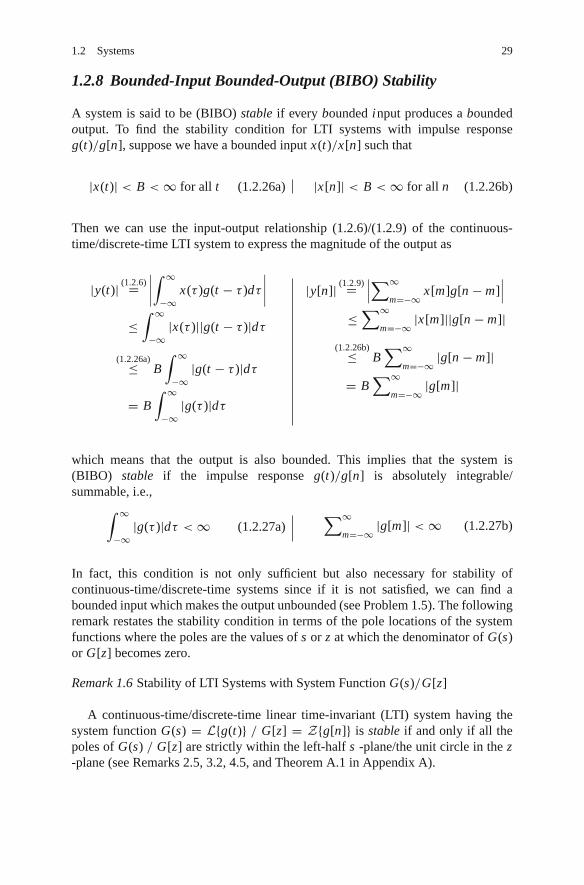
1.2 Systems 29
1.2.8 Bounded-Input Bounded-Output (BIBO) Stability
A system is said to be (BIBO) stable if every bounded input produces a boundedoutput. To find the stability condition for LTI systems with impulse responseg(t)/g[n], suppose we have a bounded input x(t)/x[n] such that
|x(t)| < B < ∞ for all t (1.2.26a) |x[n]| < B < ∞ for all n (1.2.26b)
Then we can use the input-output relationship (1.2.6)/(1.2.9) of the continuous-time/discrete-time LTI system to express the magnitude of the output as
|y(t)| (1.2.6)=∣∣∣∣∫ ∞
−∞x(τ )g(t − τ )dτ
∣∣∣∣≤∫ ∞
−∞|x(τ )||g(t − τ )|dτ
(1.2.26a)≤ B∫ ∞
−∞|g(t − τ )|dτ
= B∫ ∞
−∞|g(τ )|dτ
|y[n]| (1.2.9)=∣∣∣∑∞
m=−∞ x[m]g[n − m]∣∣∣
≤∑∞
m=−∞ |x[m]||g[n − m]|(1.2.26b)≤ B
∑∞m=−∞ |g[n − m]|
= B∑∞
m=−∞ |g[m]|
which means that the output is also bounded. This implies that the system is(BIBO) stable if the impulse response g(t)/g[n] is absolutely integrable/summable, i.e.,∫ ∞
−∞|g(τ )|dτ < ∞ (1.2.27a)
∑∞m=−∞ |g[m]| < ∞ (1.2.27b)
In fact, this condition is not only sufficient but also necessary for stability ofcontinuous-time/discrete-time systems since if it is not satisfied, we can find abounded input which makes the output unbounded (see Problem 1.5). The followingremark restates the stability condition in terms of the pole locations of the systemfunctions where the poles are the values of s or z at which the denominator of G(s)or G[z] becomes zero.
Remark 1.6 Stability of LTI Systems with System Function G(s)/G[z]
A continuous-time/discrete-time linear time-invariant (LTI) system having thesystem function G(s) = L{g(t)} / G[z] = Z{g[n]} is stable if and only if all thepoles of G(s) / G[z] are strictly within the left-half s -plane/the unit circle in the z-plane (see Remarks 2.5, 3.2, 4.5, and Theorem A.1 in Appendix A).

30 1 Signals and Systems
1.2.9 Causality
A signal x(t)/x[n] is said to be causal if it is zero for all t < 0 / n < 0. A system issaid to be causal or non-anticipatory if the response (output) of the system does notprecede the excitation (input), i.e., the output depends only on the present and pastvalues of the input. In other words, the output of a causal system to an input appearsonly while or after the input is applied to the system. The necessary and sufficientcondition for the system causality is that the impulse response is causal, i.e.,
g(t) = 0 for all t < 0 (1.2.28a) g[n] = 0 for all n < 0 (1.2.28b)
since the impulse response g(t) / g[n] means the output measured at time t [s]/ n[samples] after the impulse signal is applied as an input.
We can use Eqs. (1.2.6)/(1.2.10) (with Eqs. (1.2.7)/(1.2.11)) to write the time-domain input-output relationships of continuous-time/discrete-time causal LTI sys-tems as
y(t) =∫ ∞
−∞x(τ )g(t − τ )dτ
g(t−τ )=0 for t−τ<0=causal
∫ t
−∞g(τ )x(t − τ )dτ
=∫ t0
−∞x(τ )g(t − τ )dτ +
∫ t
t0
x(τ )g(t − τ )dτ ;
y(t) = y(t0) +∫ t
t0
x(τ )g(t − τ )dτ (1.2.29a)
y[n] =∑∞
m=−∞ x[m]g[n − m]
g[n−m]=0 for n−m<0=causal
∑n
m=−∞ x[m]g[n − m]
=∑n0
m=−∞ x[m]g[n − m]
+∑n
m=n0+1x[m]g[n − m];
y[n] = y[n0] +∑n
m=n0+1x[m]g[n − m]
(1.2.29b)
In fact, all physical systems such as analog filters are causal in the sense that theydo not react to any input before it is applied to them. As a contraposition, a non-causal or anticipatory system is not physically realizable. Causal filters are typicallyemployed in applications where the inputs are (on-line) processed as they arrive. Anexample of non-causal system is a digital filter for image processing, which collectsthe input data x[m, n]’s in one frame for some period and processes them at a timewhere m and n are spatial indices.
1.2.10 Invertibility
A system is said to be invertible if distinct inputs produce distinct outputs. If asystem G is invertible, then it is possible to design its inverse system H which,connected in cascade with G at the output port, receives the output of G to restorethe input (applied to G) as its output.
Especially for an LTI system G with the impulse response g(t)/g[n], the impulseresponse h(t)/h[n] of its inverse system H must satisfy the following condition:(see Problem 1.6)

1.3 Systems Described by Differential/Difference Equations 31
g(t)∗h(t) = δ(t); G(s)H (s) = 1 (1.2.30a)
g[n]∗h[n] = δ[n]; G[z]H [z] = 1 (1.2.30b)
(cf.) An example of non-invertible system is a gambler (with a poker face) whoseface (output) does not vary with his card (input) so that other gamblers cannotmake the inverse system reading his card from his face.
1.3 Systems Described by Differential/Difference Equations
1.3.1 Differential/Difference Equation and System Function
The time-domain input-output relationships of continuous-time/discrete-time sys-tems are often described by linear constant-coefficient differential/difference equa-tions that are set up based on underlying physical laws or design specifications tomake it perform desired operations:
∑N
i=0ai
di y(t)
dti=∑M
j=0b j
d j x(t)
dt j
with the initial conditions
y(t0), y′(t0), · · · , y(N−1)(t0)
∑N
i=0ai y[n − i] =
∑M
j=0b j x[n − j]
with the initial conditions
y[n0], y[n0 − 1], · · · , y[n0 − N + 1]
With zero initial conditions, this can be transformed to make the system or transferfunction as
∑N
i=0ai s
i Y (s) =∑M
j=0b j s
j X (s)
A(s)Y (s) = B(s)X (s);
G(s) = Y (s)
X (s)= B(s)
A(s)(1.3.1a)
where
A(s) =∑N
i=0ai s
i , B(s) =∑M
j=0b j s
j
∑N
i=0ai z
−i Y [z] =∑M
j=0b j z
− j X [z]
A[z]Y [z] = B[z]X [z];
G[z] = Y [z]
X [z]= B[z]
A[z](1.3.1b)
where
A[z] =∑N
i=0ai z
−i , B[z] =∑M
j=0b j z
− j
Note the following:- The poles/zeros of the system function G(s) or G[z] are the values of s or z at
which its denominator/numerator becomes zero.

32 1 Signals and Systems
- The degree N of the denominator A(s)/A[z] of the system function G(s)/G[z] iscalled the order of the system. If N �= 0, the system is said to be recursive in thesense that its output depends on not only the input but also the previous output;otherwise, it is said to be non-recursive or memoryless and its output dependsonly on the input.
- Especially, discrete-time recursive and non-recursive systems are called IIR(infinite-duration impulse response) and FIR ( f inite-duration impulse response)systems, respectively since the duration of the impulse response of recursive/non-recursive system is infinite/finite, respectively.
1.3.2 Block Diagrams and Signal Flow Graphs
Systems are often described by graphical means such as block diagrams or sig-nal flow graphs. As an example, let us consider an RC circuit or its equivalentdepicted in Fig. 1.16(a). We can apply Kirchhoff’s current law to write the nodeequation, take its Laplace transform with zero initial conditions, and find the systemfunction as
Input voltagesource
(a) An RC circuit and its equivalent with the voltage-to-current source transformation
vi (t)
Vi (s) Vo(s) Vi [z] I [z]
i [n]
I [z]
i [n]
vi [n]
Vi [z]
Vi [z]
vi [n]
Vo [z]
vo [n]
Vo [z]
Vo [z]
vo [n]
vo(t )
Vo (s)
Vo (s)
vo (t )
I (s)
i (t)
I (s)
i (t)
Vi –Vo Vi –Vo
vi –vovi –vovi (t)
Vi (s)
vi (t)
vo(t ) vi (t) vo (t )Ci (t )+
+
(b1) Block diagram representation
(c1) Signal flow graph representation
(d1) State diagram (d2) State diagram
(c2) Signal flow graph representation
(b2) Block diagram representation
–
–
+
–
R
R Cs
R C
11R1
C (1–z –1)Tz –1
C (1–z –1)Tz –1
adder adder
adder
1/R 1/R
T/RC
1/Cs
I (s)Vi (s) adder 1/R 1/C s –1 z –1
–1
–1–1
–1
R
Fig. 1.16 Block diagram, signal flow graph, and state diagram representations of a system

1.3 Systems Described by Differential/Difference Equations 33
Cdvo(t)
dt+ vo(t)
R= vi (t)
R(1.3.2a)
Laplace transform→B.7(5)
CsVo(s) + 1
RVo(s) = 1
RVi (s) → G(s) = Vo(s)
Vi (s)= 1
RCs + 1
(1.3.3a)
We may replace the derivative dvo(t)/dt with its difference approximation
dvo(t)
dt∼= vo((n + 1)T ) − vo(nT )
T= vo[n + 1] − vo[n]
T
with sampling interval T to discretize the differential equation into a differenceequation, take its z -transform with zero initial conditions, and find the systemfunction as
Cvo[n + 1] − vo[n]
T+ vo[n]
R= vi [n]
R(1.3.2b)
z−transform→B.7(2)
CzVo[z] − Vo[z]
T+ 1
RVo[z] = 1
RVi [z]
→ G[z] = Vo[z]
Vi [z]= 1
RC(z − 1)/T + 1(1.3.3b)
Fig. 1.16(b1)/(b2) show the block diagram representing the continuous-time/discrete-time system whose input-output relationship is described by Eqs. (1.3.2a)/(1.3.2b) in the time domain and (1.3.3a)/(1.3.3b) in the s- / z -domain.Figure 1.16(c1)/(c2) and (d1)/(d2) show their signal flow graph representationswhere a branch from node j to node i denotes the causal relationship that thesignal j is multiplied by the branch gain and contributes to the signal i . Espe-cially, Fig. 1.16(d1) is called a continuous-time state diagram since all branch gainsare constants or s−1 (denoting an integrator). Likewise, Fig. 1.16(d2) is called adiscrete-time state diagram since all branch gains are constants or z−1 (denoting adelay T ).
Since signal flow graphs are simpler to deal with than block diagrams, we willrather use signal flow graphs than block diagrams. A signal flow graph was origi-nally introduced by S.J. Mason as a graphical means of describing the cause-effectrelationship among the variables in a set of linear algebraic equations. It consists ofnodes connected by line segments called branches. Each node represents a signal(variable), whose value is the sum of signals coming along all the branches fromother nodes and being multiplied by the branch gain. Every branch has the gain anddirection that determine or are determined by the cause-effect relationship amongthe variables denoted by its nodes. Note that a branch with no gain indicated issupposed to have unity gain.

34 1 Signals and Systems
For example, we consider the following set of linear equations:
y2 = a12 y1 + a32 y3, y3 = a23 y2 + a43 y4,
y4 = a34 y3 + a44 y4 + a54 y5, y5 = a25 y2 + a35 y3 + a45 y4
which describes the cause-effect relationship among the variables y1, y2, y3, y4,and y5 with the causes/effects in the right/left-hand side, respectively. Figure 1.17shows a signal flow graph representing the relationships described by this set ofequations.
Inputnode
Outputnodey1 y2 y3 y4 y5 y5a12 a23 a34
a44
a43a32
a35a54
a25
a45
1
Fig. 1.17 A signal flow graph
1.3.3 General Gain Formula – Mason’s Formula
In this section we introduce Mason’s gain formula, which is applied to signal flowgraphs to yield the overall gain from an input node to an output node. To understandhow to use the formula, we need to know the following terms:
- Input Node (Source) : A node having only outgoing branches.- Output Node (Sink) : A node having only incoming branches.
(cf.) Note that, in contrast with the input node, the output node may not be clearlyseen. Suppose we don’t have the dotted branch in the signal flow graphdepicted in Fig. 1.17. In that case, if we regard y5 as an output, we maydraw a branch with unity gain from the node for y5 so that the node appearsto be an output node.
- Path: A continuous connection of branches traversed in the same direction.- Forward Path: A path connecting an input node to an output node along which
no node is encountered more than once.- Loop: A closed path that originates and terminates at the same node and encoun-
ters no other node more than once.- Path Gain: The product of all the branch gains along a path.- Loop Gain: The path gain of a loop.- Non-touching: Having no nodes in common.
The gain formula states that the overall gain is
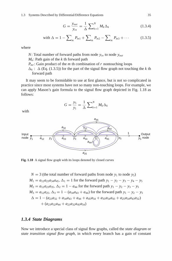
1.3 Systems Described by Differential/Difference Equations 35
G = yout
yin= 1
Δ
∑N
k=1MkΔk (1.3.4)
with Δ = 1 −∑
mPm1 +
∑m
Pm2 −∑
mPm3 + · · · (1.3.5)
where
N : Total number of forward paths from node yin to node yout
Mk : Path gain of the k th forward pathPmr : Gain product of the m th combination of r nontouching loopsΔk : Δ (Eq. (1.3.5)) for the part of the signal flow graph not touching the k th
forward path
It may seem to be formidable to use at first glance, but is not so complicated inpractice since most systems have not so many non-touching loops. For example, wecan apply Mason’s gain formula to the signal flow graph depicted in Fig. 1.18 asfollows:
G = y5
y1= 1
Δ
∑N
k=1MkΔk
with
Inputnode
Outputnodey1 y2 y3 y4 y5 y5a12 a23 a34
a44
a43a32
a35
a54
a25
a45
1
Fig. 1.18 A signal flow graph with its loops denoted by closed curves
N = 3 (the total number of forward paths from node y1 to node y5)
M1 = a12a23a34a45,Δ1 = 1 for the forward path y1 − y2 − y3 − y4 − y5
M2 = a12a23a35,Δ2 = 1 − a44 for the forward path y1 − y2 − y3 − y5
M3 = a12a25,Δ3 = 1 − (a34a43 + a44) for the forward path y1 − y2 − y5
Δ = 1 − (a23a32 + a34a43 + a44 + a45a54 + a35a54a43 + a25a54a43a32)
+ (a23a32a44 + a23a32a45a54)
1.3.4 State Diagrams
Now we introduce a special class of signal flow graphs, called the state diagram orstate transition signal flow graph, in which every branch has a gain of constant

36 1 Signals and Systems
or s−1 (integrator)/z−1 (delay). This is very useful for the purposes of systemanalysis, design, realization, and implementation. Systems represented by the statediagram need the following three basic software operations or hardware elementsfor implementation:
- addition(adder) - addition- multiplication(amplifier) - multiplication- integration(integrator) s−1 - delay (z−1)/advance (z)
It is good enough to take a look at the following examples.
Example 1.4a Differential Equation and Continuous-Time State Diagram
Figure 1.19(a) and (b) show the controllable and observable form of state dia-grams, respectively, both of which represent the following differential equation orits Laplace transform (see Problem 1.9):
y′′(t) + a1 y′(t) + a0 y(t) = b1u′(t) + b0u(t) with zero initial conditions(E1.4a.1)
(s2 + a1s + a0)Y (s) = (b1s + b0)U (s) (E1.4a.2)
Example 1.4b Difference Equation and Discrete-Time State Diagram
Figure 1.20(a)/(b)/(c)/(d) show the direct I/transposed direct I/direct II/transposeddirect II form of state diagrams, respectively, all of which represent the followingdifference equation or its z -transform (see Problems 1.8 and/or 8.4):
y[n + 2] + a1 y[n + 1] + a0 y[n] = b1u[n + 1] + b0u[n] with zero initial conditions(E1.4b.1)
(z2 + a1z + a0)Y [z] = (b1z + b0)U [z] (E1.4b.2)
(b) Observable canonical form of state diagram
(a) Controllable canonical form of state diagram
U (s)u (t)
U (s)u (t)
Y (s)y (t )
Y (s)y (t )
x2x2x2
x1
x2 = –a0x1 – a1x2 + u
–a1
–a1
b1
–a0
–a0
b0
x1 b0
x1
b1
x2s–1
s–1
: Integrators–1
s–1
s–1x2′
x1
x1′ ′
′
′
x2 = x1–a1x2 + b1u′
x1 = –a0x2 + b0u′
y = b0x1 + b1x2x1′ = x2
y = x2
: Adder(addition)
: Amplifier (multiplication)b
: Signal distribution point
Fig. 1.19 State diagrams for a given differential equation y′′(t)+a1 y′(t)+a0 y(t) = b1u′(t)+b0u(t)
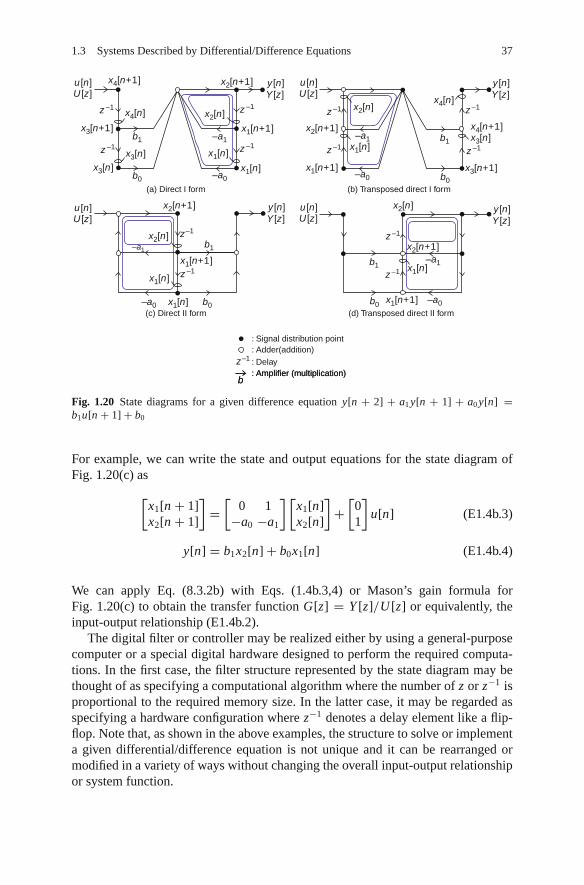
1.3 Systems Described by Differential/Difference Equations 37
U [z]u [n]
U [z]u [n]
U [z]u [n]
Y [z]y [n]
Y [z]y [n]
Y [z]y [n]
U [z]u [n]
Y [z]y [n]
x2[n]x2[n]
x2[n]
x1[n]
x4[n]
x2[n]
x2[n+1]
x2[n+1]
x4[n+1]
x3[n+1] x1[n+1] x2[n+1] x4[n+1]
x3[n+1]
x1[n+1]
x2[n+1]
x1[n+1]
x1[n+1]
x1[n]
x1[n]x1[n]
x3[n]
x4[n]
x1[n]
x1[n]
x3[n]x3[n]
b1
b1
b0
b0
–a1 –a1
–a0 b0
b0
b1
b1
–a0
–a0
–a1
–a0
–a1
z –1
z –1
z –1z –1 z –1
z –1z –1
z –1
z –1
z –1
z –1
z–1
(c) Direct II form (d) Transposed direct II form
(a) Direct I form (b) Transposed direct I form
b: Amplifier (multiplication)
z–1 : Delay
: Signal distribution point: Adder(addition)
b: Amplifier (multiplication)
Fig. 1.20 State diagrams for a given difference equation y[n + 2] + a1 y[n + 1] + a0 y[n] =b1u[n + 1] + b0
For example, we can write the state and output equations for the state diagram ofFig. 1.20(c) as
[x1[n + 1]x2[n + 1]
]=[
0 1−a0 −a1
] [x1[n]x2[n]
]+[
01
]u[n] (E1.4b.3)
y[n] = b1x2[n] + b0x1[n] (E1.4b.4)
We can apply Eq. (8.3.2b) with Eqs. (1.4b.3,4) or Mason’s gain formula forFig. 1.20(c) to obtain the transfer function G[z] = Y [z]/U [z] or equivalently, theinput-output relationship (E1.4b.2).
The digital filter or controller may be realized either by using a general-purposecomputer or a special digital hardware designed to perform the required computa-tions. In the first case, the filter structure represented by the state diagram may bethought of as specifying a computational algorithm where the number of z or z−1 isproportional to the required memory size. In the latter case, it may be regarded asspecifying a hardware configuration where z−1 denotes a delay element like a flip-flop. Note that, as shown in the above examples, the structure to solve or implementa given differential/difference equation is not unique and it can be rearranged ormodified in a variety of ways without changing the overall input-output relationshipor system function.

38 1 Signals and Systems
1.4 Deconvolution and Correlation
In this section we will introduce the two terms related with the convolution. One isthe deconvolution, which is the inverse process of convolution. The other is the cor-relation, which is procedurally similar to, but totally different from the convolutionin the physical meaning and usage.
1.4.1 Discrete-Time Deconvolution
In Sect. 1.2.3, the input-output relationship of a discrete-time LTI (linear time-invariant) system was derived as Eq. (1.2.9):
y[n](1.2.9)= g[n]∗x[n] =
∑∞m=−∞ g[n − m]x[m] (1.4.1)
where x[n], y[n], and g[n] are the input, output, and impulse response of thesystem. Thus, for an FIR ( f inite-duration impulse response) system with
g[n] = 0 for |n| ≥ N , (1.4.2)
we can write its output to the input {x[m] for m = 0 : N − 1} applied from m = 0to N − 1 as
y[n] =∑N−1
m=0g[n − m]x[m] (1.4.3)
or in matrix-vector form as
⎡⎢⎢⎢⎣
y[0]
y[1]
•y[N − 1]
⎤⎥⎥⎥⎦ =
⎡⎢⎢⎢⎣
g[0] g[−1] • g[−N + 1]
g[1] g[0] • g[−N + 2]
• • • •g[N − 1] g[N − 2] • g[0]
⎤⎥⎥⎥⎦⎡⎢⎢⎣
x[0]x[1]•
x[N − 1]
⎤⎥⎥⎦ ;
y = Gx with G : transmission matri x (1.4.4)
One might ask a question, “Can we or how can we find the input sequence x[n]for a system characterized by its impulse response g[n] to produce a certain outputsequence y[n]?”. For the FIR system with the input-output relationship describedby Eq. (1.4.4), we can find the input sequence as
x = G−1y, (1.4.5)
if the transmission matrix G is nonsingular. Furthermore, if the system is causal,i.e., g[n] = 0 for n < 0, then the transmission matrix becomes lower-triangular as

1.4 Deconvolution and Correlation 39
G =
⎡⎢⎢⎢⎣
g[0] 0 · 0
g[1] g[0] · 0
· · · ·g[N − 1] g[N − 2] · g[0]
⎤⎥⎥⎥⎦ (1.4.6)
so that if g[0] �= 0, the input sequence can be determined by forward substitution:
x[n] = y[n] − ∑n−1m=0 g[n − m]x[m]
g[0](1.4.7)
starting from x[0] = y[0]/g[0] (see Problem 1.11).Note that the problem of determining the impulse response g[n] for given input
and output sequences can be dealt with in the same way.
1.4.2 Continuous/Discrete-Time Correlation
The cross-correlation between two signals measures how similar the two signals areover temporal or spatial difference. The auto-correlation of a signal measures howmuch the signal looks like itself over temporal or spatial difference. Correlationis widely used for various purposes including signal detection in communicationsystems.
Let x(t)/x[n] and y(t)/y[n] be two continuous-time/discrete-time transient orfinite-duration signals. Then the cross-correlation between them is defined as fol-lows:
φxy(τ ) =∫ ∞
−∞x(t + τ )y∗(t)dt
=∫ ∞
−∞x(t)y∗(t − τ )dt
=∫ ∞
−∞x(−t + τ )y∗(−t)dt
(1.4.8a)
φxy[m] =∑∞
n=−∞ x[n + m]y∗[n]
=∑∞
n=−∞ x[n]y∗[n − m]
=∑∞
n=−∞ x[−n + m]y∗[−n]
(1.4.8b)
where τ/m, called a lag variable, represents the relative delay (shift) between thetwo signals. If the two signals happen to be identical, i.e., x(t) = y(t)/x[n] = y[n],we have the auto-correlation as

40 1 Signals and Systems
φxx (τ ) =∫ ∞
−∞x(t + τ )x∗(t)dt
=∫ ∞
−∞x(t)x∗(t − τ )dt
=∫ ∞
−∞x(−t + τ )x∗(−t)dt
(1.4.9a)
φxx [m] =∑∞
n=−∞ x[n + m]x∗[n]
=∑∞
n=−∞ x[n]x∗[n − m]
=∑∞
n=−∞ x[−n + m]x∗[−n]
(1.4.9b)
There are some properties of correlation to note:
φxx (τ ) = φ∗xx (−τ ) (1.4.10a)
φxy(τ ) = φ∗yx (−τ ) (1.4.11a)
φxy(τ ) = x(τ )∗y∗(−τ ) (1.4.12a)
φxx [m] = φ∗xx [−m] (1.4.10b)
φxy[m] = φ∗yx [−m] (1.4.11b)
φxy[m] = x[m]∗y∗[−m] (1.4.12b)
If x(t)/x[n] and y(t)/y[n] are the input and output of a continuous-time/discrete-time LTI system so that y(t) = g(t) ∗ x(t)/y[n] = g[n] ∗ x[n], then we have
φxy(τ ) = g∗(−τ )∗φxx (τ ) (1.4.13a)
φyy(τ ) = g∗(−τ )∗φyx (τ ) (1.4.14a)
φxy[m] = g∗[−m]∗φxx [m] (1.4.13b)
φyy[m] = g∗[−m]∗φyx [m] (1.4.14b)
(cf.) If the signals are random or periodic so that nonzero values appear allover the time interval, the correlation should be defined as a time-averageversion.
The correlation functions are very useful for extracting certain signals from noisyones and determining the spectral density of random signals. Look at the followingremark and example.
Remark 1.7 Properties of Autocorrelation
(1) In case two signals are periodic or random, their correlation should be defined as
φxy(τ ) = 1
2T
∫ T
−Tx(t + τ )y∗(t)dt
(1.4.15a)
φxy[m] = 1
2N + 1
∑N
n=−Nx[n + m]y∗[n]
(1.4.15b)
(2) The autocorrelation (1.4.9a)/(1.4.9b) is even and has its maximum at τ =0/m = 0. In the case of periodic or random signals, the maximum value isthe mean squared value of the signal.

1.4 Deconvolution and Correlation 41
Remark 1.8 Convolution vs. Correlation and Matched Filter
(1) Equation (1.2.7)/(1.2.11) implies that the continuous-time/discrete-time con-volution of two time functions/sequences can be obtained by time-reversingone of them and time-shifting (sliding) it, multiplying it with the other, andthen integrating/summing the multiplication. The correlation differs from theconvolution only in that the time-reversal is not performed.
(2) If we time-reverse one of two signals and then take the convolution of the time-reversed signal and the other one, it will virtually yield the correlation of theoriginal two signals since time-reversing the time-reversed signal for comput-ing the convolution yields the original signal as if it had not been time-reversed.This presents the idea of matched filter, which is to determine the correlationbetween the input signal x(t)/x[n] and a particular signal w(t)/w[n] based onthe output of the system with the impulse response g(t) = w(−t)/g[n] =w[−n] to the input x(t)/x[n]. This system having the time-reversed and pos-sibly delayed version of a particular signal as its impulse response is called thematched filter for that signal. Matched filter is used to detect a signal, i.e., todetermine whether or not the signal arrives and find when it arrives.
Example 1.5 Correlation and Matched Filter
Consider the two signal waveforms of duration T = 2 [s], which represent0 and 1 and are depicted in Fig. 1.21(a1) and (b1), respectively. According toRemark 1.8(2), the impulse responses of their matched filters are
0
0 1 2 3 4 5 6 7 8 9 10
0 1 2 3 4 5 6 7 8 9 10
0 1 2 3 4 5 6 7 8 9 10
11
(a1) x1(t )
x1(t )
y1(t )
y2(t )
(b1) x2(t )
(c) An input signal x (t )
(d1) The output y1(t ) of matched filter 1 to the input depicted in (c)
(d2) The output y2(t ) of matched filter 2 to the input depicted in (c)
(a2) g1(t ) = x1(T–t ) (b2) g2(t ) = x2(T–t )
1
1
2 0 1 2 0
0
1 1
–1
1
2 2t t t t
t
t
t
Fig. 1.21 Two matched filters for two signals and their outputs to an input signal

42 1 Signals and Systems
g1(t) = x1(−t) and g2(t) = x2(−t) (E1.5.1)
We have, however, a problem that these filters are non-causal so that they are notphysically realizable. A reasonable measure is to shift their impulse responses byT = 2 so that they become causal as depicted in Fig. 1.21(a2) and (b2):
g1(t) = x1(T − t) and g2(t) = x2(T − t) (E1.5.2)
Suppose the input signal depicted in Fig. 1.21(c) is applied to the two matchedfilters with the impulse responses given by (E1.5.2). We can compose the followingMATLAB program “sig01e05.m” to find their outputs and run it to get the resultsshown in Figs. 1.21(d1) and (d2). There are some points to think about:
- As long as the amplitude of the signals (expected to arrive) are the same, theoutput of each matched filter achieves its maximum 2 s after the correspondingsignal arrives. Why?
%sig01e05.m% Correlation/Convolution and Matched Filterclear, clfM=50; Ts=1/M;x1=ones(M,1)*[1 1]; x1=x1(:).’; Nx=length(x1);x2=ones(M,1)*[1 -1]; x2=x2(:).’;g1=fliplr(x1); g2=fliplr(x2);x=[x1 zeros(1,M) x2 zeros(1,M) x1 zeros(1,M) x2]; % signal to transmitlength x=length(x); Nbuffer= min(M*11,length x); tt=[0:Nbuffer-1]*Ts;% Noise amp=0.3; x = x + Noise amp*randn(1,length x);xbuffer=zeros(1,Nbuffer); ybuffer=zeros(2,Nbuffer);for n=1:length x
xbuffer= [x(n) xbuffer(1:end-1)];y= [g1; g2]*xbuffer(1:Nx).’*Ts; ybuffer= [ybuffer(:,2:end) y];subplot(312), plot(tt,ybuffer(1,:)), subplot(313), plot(tt,ybuffer(2,:))pause(0.01), if n<length x, clf; end
endy1=xcorr(x,x1)*Ts; y1=y1([end-Nbuffer+1:end]-Nx); %correlation delayed by Nxy2=xcorr(x,x2)*Ts; y2=y2([end-Nbuffer+1:end]-Nx);subplot(312), hold on,plot(tt,y1,’m’) % only for cross-checksubplot(313), hold on, plot(tt,y2,’m’)
- If we remove the zero period between the signals and generate a signal every 2 sin the input, could we still notice the signal arrival times from (local) maxima ofthe output? (See Problem 1.12(a).)
Remark 1.9 xcorr() – MATLAB function for Correlation
(1) The MATLAB function xcorr(x,y) returns the correlation of two sequencesx[n] and y[n] defined by Eq. (1.4.16). Depending on the third input argument,it returns different versions of correlation as follows:

1.4 Deconvolution and Correlation 43
xcorr(x,y,’coeff’) →
ρxy[m] =∑∞
n=−∞ x[n + m] y∗[n]
(∑ |x[n]|2 ∑ |y[n]|2)1/2
(−1 ≤ ρ ≤ +1)
(correlation coefficient) (1.4.16a)
xcorr(x,y,’biased’) →
ϕxy[m] =⎧⎨⎩
1N
∑N−1−|m|n=0 x[n + m] y∗[n] for 0 ≤ m ≤ N − 1
1N
∑N−1−|m|n=0 x[n] y∗[n − m] for − (N − 1) ≤ m ≤ 0
(1.4.16b)
xcorr(x,y,’unbiased’) →
ϕxy[m] =⎧⎨⎩
1N−|m|
∑N−1−|m|n=0 x[n + m] y∗[n] for 0 ≤ m ≤ N − 1
1N−|m|
∑N−1−|m|n=0 x[n] y∗[n − m] for − (N − 1) ≤ m ≤ 0
(1.4.16c)
(2) If the two sequences are of different lengths, xcorr(x,y) appends one ofthem by zeros to make them have equal lengths and returns theirconvolution.
(3) The durations of the convolution and correlation of two sequences x[n] (of dura-tion [n0 x :n f x ]) and y[n] (of duration [n0 y :n f y]) are [n0 x +n0 y :n f x +n f y]and [n0 x − n f y :n f x − n0 y], respectively.
Example 1.6 Correlation for Periodic Signals with Random Noise
We can use MATLAB function randn(M,N) to generate a zero-mean and unit-variance normal (Gaussian) noise sequence in an M × N matrix. Figure 1.22(a1)and (a2) illustrate a Gaussian 1 × 128 random sequence w[n] with variance σ 2 =0.52 (generated by 0.5*randn(1,N)) and its autocorrelation φww[m] (obtainedby xcorr(w,w)), respectively. On the other hand, Fig. 1.22(b1) shows a noise-contaminated sinusoidal sequence x[n] = sin(πn/16) + w[n]. Figure 1.22(b2),(b3), and (b4) show the various autocorrelations of x[n] that are obtained byusing xcorr(w,w), xcorr(w,w,‘coef’)/xcorr(w,w, ‘biased’),and xcorr(w,w,‘unbiased’), respectively.
Note the following observations:
- All the autocorrelations in Fig. 1.22(a2), (b2)–(b4) are even and have their max-ima at m = 0 as stated in Remark 1.7(2). Especially, the maximum of φww[m] inFig. 1.22(a2) is

44 1 Signals and Systems
2
0
–2
2
0
–2
–1
0
1
–1
0
1
0 100
0 100
–100
0
20
40
–50 0 50 100
–100–100
0
100
–50 0 50 100
–100 –50 0 50 100–100 –50 0 50 100
: coef: biased
(a1) A (Gaussian) noise sequence w [n] (a2) Autocorrelation of w [n]
(b1) A noise-contaminated sinusoidal wave x [n] (b2) Autocorrelation of x [n] from xcorr( )
(b3) Autocorrelation of x [n]from xcorr(x,x, ‘biased’)/xcorr(x,x, ‘coef’)
(b4) Autocorrelation of x [n]from xcorr(x,x, ‘unbiased’)
Fig. 1.22 Autocorrelation obtained using the MATLAB function xcorr()
φww[0] � Expectation
{∑N−1
n=0x2[n]
}�∑N−1
n=0σ 2 = 128 × 0.52 = 32
(E1.6.1)- Marvelously, the noise effect can hardly be found in the autocorrelation except
for the spike at m = 0. Thanks to the noise reduction effect of autocorrelation, theperiodicity of the signal can be observed more clearly from the autocorrelationthan from the original noise-contaminated signal.
- Figure 1.22(b2) and (b3) show that the autocorrelation obtained fromxcorr(w,w,‘biased’) is just a 1/N -scaled version of that obtained fromxcorr(w,w). The normalized version obtained from xcorr(w,w,‘coef’)has similar shape. Any of these versions have some end effect, i.e., their magni-tudes decrease as the time lag m increases not because the correlation or similar-ity gets loose, but because the number of samples in the summation decreases.In contrast, the autocorrelation obtained from xcorr(w,w,‘unbiased’) isrelatively free from the end effect as shown in Fig. 1.22(b4).
%sig01e06.m : Autocorrelation of a noise-contaminated periodic signalN=128; W=pi/16; nn=0:N-1;s= sin(W*nn); w= 0.5*randn(1,N); x=s+w;subplot(321), plot(nn,w)[phi w,mlag]=xcorr(w,w); % Autocorrelation of the noisesubplot(322), plot(mlag,phi w)

Problems 45
subplot(323), plot(nn,x, nn,s,’k’)[phi x,mlag]=xcorr(x,x); % Autocorrelation of the corrupted signalsubplot(324), plot(mlag,phi x)[phi x coef,mlag]=xcorr(x,x,’coef’); % Correlation coefficientsubplot(325), plot(mlag,phi x coef)[phi x biased,mlag]=xcorr(x,x,’biased’); % Biased autocorrelationhold on, plot(mlag,phi x biased,’r:’)[phi x unbiased,mlag]=xcorr(x,x,’unbiased’); % Unbiased autocorrelationsubplot(326), plot(mlag,phi x unbiased),axis([mlag([1 end]) -1 1])
1.5 Summary
In this chapter we have introduced some basic continuous-time/discrete-time signalsand defined a number of important concepts related to systems such as linearity,time-invariance, causality, stability, impulse response, and system (transfer) func-tion. We have also derived the convolution form of input-output relationship of LTIsystems. We have also indicated that a continuous-time/discrete-time system can bedescribed analytically by differential/difference equations and pictorially by signalflow graphs. Finally, we introduced the concept of correlation.
Problems
1.1 Representation of Unit Impulse Function by Sinc Function
(a) Referring to the web site <http://mathworld.wolfram.com/SincFunction.html> or [K-1] (Sect. 15.4, Example 2) or Eq. (E2.3.3) of this book, showthat the sinc function representation (1.1.33a) of the unit impulse functionδ(t) satisfies the property (1.1.19) regardless of D or w:
∫ ∞
−∞
w
π
sin(wt)
wtdt
wt→x= 1
π
∫ ∞
−∞
sin(x)
xdx = 1 (P1.1.1)
(b) Plot the sinc function1
Dsinc
(t
D
)= sin(π t/D)
π t(P1.1.2)
against time t for D = 1, 0.5, 0.25, and 0.125 and check the following:
- It is an even function since both of the numerator and denominatorfunctions are odd ones.
- Its amplitude decreases as |t | increases since the magnitude of thedenominator increases while the amplitude of the numerator is constant.
- It becomes zero at t = m D(m �= 0) and 1/D at t = 0 sincelimx→0
sinc(x) = 1.

46 1 Signals and Systems
1.2 ConvolutionConsider the two continuous-time signals x(t) = r3(t) = us(t) − us(t − 3) andg(t) = e−0.5t us(t).
(a) Show that the (continuous-time) convolution of these two signals is
x(t)∗g(t) =
⎧⎪⎨⎪⎩
0 for t < 0
2(1 − e−0.5t ) for 0 ≤ t < 3
2(e−0.5(t−3) − e−0.5t ) = 2(e1.5 − 1)e−0.5t for t ≥ 3(P1.2.1)
(b) As in Example 1.2, we can use the MATLAB function ‘conv ()’ to com-pute this continuous-time convolution approximately. Compose a programwhich samples the two signals at t = nTs(Ts = 0.1[s]), use ‘conv ()’ tocompute the convolution, and plot it together with the true convolution(P1.2.1) for t = [0, 10]s. Run it to see if the approximate convolu-tion is close to the true one. If we decrease the sampling period, say, toTs = 0.01 s, is it helpful?
1.3 Necessary Condition on BIBO (Bounded Input Bounded Output) StabilityIn Sect. 1.2.8 it was shown that the absolute integrability/summability(1.2.27a)/(1.2.27b) of impulse response guarantees the BIBO stability and thusare sufficient conditions. Here, you can show that if the conditions do not hold,there is a bounded input yielding unbounded output, which implies that theyare also necessary conditions for BIBO stability. To this end, suppose that theimpulse response of a system does not satisfy the condition (1.2.27a)/(1.2.27b):
∫ ∞
−∞|g(τ )|dτ = ∞ (P1.3.1a)
∑∞m=−∞ |g[m]| = ∞ (P1.3.1b)
(a) Consider the following signal:
x(t) ={
0 for t such that g(−t) = 0g∗(−t)|g(−t)| for t such that g(−t) �= 0
(P1.3.2a)
x[n] ={
0 for n such that g[−n] = 0g∗[−n]|g[−n]| for n such that g[−n] �= 0
(P1.3.2b)
Are these signals bounded? If they are bounded, what is their upperbound?(b) Show that the output y(t)/y[n] to the (bounded) input x(n)/x[n] at t =
0/n = 0 is unbounded, implying that the system is not BIBO stable.
1.4 Stability of Continuous-Time SystemsRemark 1.6 states that a continuous-time LTI system is stable if and only if itssystem function G(s) = L{g(t)} has all the poles strictly within the left-half s

Problems 47
-plane or equivalently, the real parts of all the poles are negative. Referring tothe remark, consider the following two systems:
Ga(s) = 2
(s + 1)(s + 2)(P1.4.1a)
Gb(s) = 6
(s − 1)(s + 2)(P1.4.1b)
(a) Find the impulse responses ga(t) and gb(t) by taking the inverse Laplacetransform of each system function. Check if each system satisfies thestability condition (1.2.27a) or not.
(b) Find the poles of each system function and determine whether or not eachsystem satisfies the stability condition stated in Remark 1.6. Does the resultagree to that obtained in (a)?
(c) Find the step responses of the two systems, i.e., their outputs to a unit-stepinput x(t) = us(t) whose Laplace transform is X (s) = 1/s. Check if eachstep response converges or not.
(cf.) You might get ya(t) by typing the following commands into the MAT-LAB command window:
>> syms s; Gas=2/(s+1)/(s+2); Xs=1/s;Yas=Gas*Xs, yat=ilaplace(Yas)
1.5 Stability of Discrete-Time SystemsRemark 1.6 states that a discrete-time LTI System is stable if and only if itssystem function G[z] = Z{g[n]} has all the poles strictly within the unit circle(see Remark 4.5). Referring to the remark, consider the following two systems:
Ga[z] = 3z
(z − 0.5)(z + 0.5)(P1.5.1a)
Gb[z] = z
(z − 1.5)(z − 0.5)(P1.5.1b)
(a) Find the impulse responses ga[n] and gb[n] by taking the inverse z -transform of each system function. Determine whether each system satisfiesthe stability condition (1.2.27b) or not.
(b) Find the poles of each system function and determine whether or not eachsystem satisfies the stability condition stated in Remark 1.6. Does the resultagree to that obtained in (a)?
(c) Find the step responses of the two systems to a unit-step input x[n] = us[n]whose z -transform is X [z] = z/(z − 1). Determine whether each stepresponse converges or not.
(cf.) You might get ya[n] by typing the following commands into the MAT-LAB command window:>> syms z; Gaz=3*z/(z−0.5)/(z+0.5); Xz=z/(z−1);
Yaz=Gaz*Xz, yan=iztrans(Yaz)

48 1 Signals and Systems
1.6 Inverse SystemConsider a model for echo generation, which is depicted in Fig. P1.6(a).
(a) Noting that the time-domain input-output relationship is
y(t) = a y(t − T ) + x(t) (P1.6.1)
show that the impulse response is
g(t) =∑∞
k=0akδ(t − kT ) with 0 < a < 1 (P1.6.2)
Also find the system function G(s) by taking the Laplace transform of thisimpulse response or the time-domain input-output relationship. Referringto Eq. (1.2.27a) or Remark 1.6, determine the stability condition of themodel system.
(b) Use Eq. (1.2.30a) to find the system function H (s) of the inverse system.Show that the inverse system can be modeled as Fig. P1.6(b), whose time-domain input-output relationship is
x(t) = y(t) − a y(t − T ) (P1.6.3)
1.7 Inverse SystemConsider a discrete-time model for duo-binary signaling, which is depicted inFig. P1.7(a).
(a) Noting that the time-domain input-output relationship is
y[n] = x[n] + x[n − 1] (P1.7.1)
find the system function G[z] by taking its z -transform.
y (t ) = ay (t–T ) + x(t )
x (t )a –a
(a) A model for echoing (b) A model for removing the echo
e–sT e–sT
y (t ) x (t )y (t )
x (t ) = y (t ) – ay (t–T )∧
∧
Fig. P1.6
y [n ] = x [n] + x [n – 1]y [n ] y [n ]x [n ]
(a) A model for duo–binary signaling (b) A model for detecting system
z –1
1 –1z
–1
x [n ]∧
x [n ] = –x [n –1 ] + y [n]∧ ∧
Fig. P1.7

Problems 49
(b) Use Eq. (1.2.30b) to find the system function H [z] of the inverse system.Show that the inverse system can be modeled as Fig. P1.7(b), whose time-domain input-output relationship is
x[n] = −x[n − 1] + y[n] (P1.7.2)
1.8 Simulation of Continuous-Time/Discrete-Time System Using MATLAB andSimulink
(a) Find the system function of the system described by the block diagram inFig. 1.16(b1) or the signal flow graph in Fig. 1.16(c1) or (d1) with RC = 1.Referring to the upper part of Fig. P1.8(a) and the parameter setting dialogboxes in Fig. P1.8(b1), (b2), and (b3), perform the Simulink simulation toplot the output signal vo(t) for 0 ≤ t < 4 s.
(a) Simulink block diagram for simulating the systems of Fig 1.16(b1) and (b2)
(b1) Parameter setting dialog box for Step and Step 1 (b2) Parameter setting dialog box for Add and Add1
Step Add Transfer Fcn Mux
Scope
DiscreteTransfer Fcn
Simulink/Sources/StepSimulink/Math Operations/AddSimulink/Continuous/Transfer FcnSimulink/Discrete/Discrete Transfer FcnSimulink/Signal Routing/MuxSimulink/Sink/ScopeStep1 Add1
+
+
–
–
1s
Tz–1
(c) The outputs obtained from the Simulink simulation
0 0.5
vo(t )vo(t )
0
0.2
0.4
0.6
0.8
1
1 1.5 2 2.5 3 3.5 4
(b3) Parameter setting dialog box for Transfer Fcn (b4) Parameter setting dialog box for Discrete Transfer Fcn
Fig. P1.8

50 1 Signals and Systems
(b) Find the system function of the system described by the block diagram inFig. 1.16(b2) or the signal flow graph in Fig. 1.16(c2) or (d2) with RC = 1.Referring to the lower part of Fig. P1.8(a) and the parameter setting dialogboxes in Fig. P1.8(b1), (b2), and (b4), perform the Simulink simulationwith sampling interval T = 0.1 to plot vo(t) for 0 ≤ t < 4 s. Also referringto the following program “sig01p 08b.m”, perform the MATLAB simula-tion to plot vo(t) for 0 ≤ t < 4 s. Does decreasing the sampling interval to,say, T = 0.01 make the output close to that of the continuous-time systemobtained in (a)?
(cf.) If you parameterize a constant such as T in the Simulink block diagramso that it can be easily changed, you can set it to a new value in theMATLAB command window.
% sig01p 08a.m% Continuous-Time System Simulation clear, clfR=1; C=1; RC=R*C; tf=4;T=0.1; tt=[0:T:tf];vi = ones(size(tt)); % step inputvo t0=0;options=odeset(’RelTol’,1e-4);vo = ode45(dvodt,tt,vo t0,options,RC);plot(tt,vo), hold on
function dv=dvodt(t,vo,RC)dv = (-vo+(t>=0))/RC;
% sig01p 08b.m% Discrete-Time System Simulationclear, clfR=1; C=1; RC=R*C; tf=4;T=0.1; tt=[0:T:tf];vi = ones(size(tt)); % step inputTRC=T/RC; vo(1)=0;for n=1:length(tt)-1
vo(n+1)=vo(n)+(vi(n)-vo(n))*TRC;endstairs(tt,vo)
1.9 Continuous-Time State Diagram, State Equation, Transfer Function, andInput-Output RelationshipWe can write the state equation for a continuous-time state diagram by takingthe following procedure.
1. Assign a state variable xi (t) to the output of each integrator s−1.2. Express the input x ′
i (t) of each integrator s−1 in terms of the statevariables and system input(s).
3. Express each output in terms of the state variables and input(s).

Problems 51
(a) Show that we can apply the above procedure to the state diagram ofFig. 1.19(a) and write the state equation together with the output equa-tion as [
x ′1(t)
x ′2(t)
]=[
0 1−a0 −a1
] [x1(t)x2(t)
]+[
01
]u(t) (P1.9.1)
y(t) = [b0 b1
] [x1(t)x2(t)
](P1.9.2)
We can also substitute the output equation (P1.9.2) into the left-hand sideof Eq. (E1.4a.1) and use the state equation (P1.9.1) to get the right-handside of Eq. (E1.4a.1):
y′′(t) + a1 y′(t) + a0 y(t) = b1u′(t) + b0u(t) (P1.9.3)
(b) Show that we can apply the above procedure to the state diagram ofFig. 1.19(b) and write the state equation together with the output equa-tion as [
x ′1(t)
x ′2(t)
]=[
0 −a0
1 −a1
][x1(t)
x2(t)
]+[
b0
b1
]u(t) (P1.9.4)
y(t) = [0 1
] [x1(t)
x2(t)
](P1.9.5)
We can also combine these state and output equations to get the input-output relationship (E1.4a.1).
(c) Apply Eq. (8.3.2a) with Eqs. (P1.9.1,2) or (P1.9.4,5) to find the transferfunction G(s) = Y (s)/U (s) or equivalently, the input-output relation-ship (E1.4a.2). Also apply Mason’s gain formula for Fig. 1.19(a) or (b)to find G(s).
(d) With a0 = 2, a1 = 3, b0 = 4, and b1 = 3, use the MATLAB func-tion ss2tf() to find the transfer function G(s) of the system describedby Eqs. (P1.9.1,2) or (P1.9.4,5). Reversely, use the MATLAB functiontf2ss() to find a state equation for the transfer function
G(s) = b1s + b0
s2 + a1s + a0= 3s + 4
s2 + 3s + 2(P1.9.6)
Which one does it yield, the equivalent of Eq. (P1.9.1,2) or (P1.9.4,5)?(e) Referring to the following program “sig01p 09.m”, simulate the systems
described by Eqs. (P1.9.1,2) and (P1.9.4,5) with a0 = 2, a1 = 3, b0 = 4,and b1 = 3 to find their outputs (y(t)’s) to an input u(t) = sin(2t) for0 ≤ t < 10 s (with sampling interval T = 0.01 s). Do the state equationsconform to each other in terms of the input-output relationship?

52 1 Signals and Systems
a0=2; a1=3; b0=4; b1=3;A1=[0 1;-a0 -a1]; B1=[0;1]; C1=[b0 b1]; [num1,den1]= ss2tf(A1,B1,C1,D1)A2=[0 -a0;1 -a1]; B2=[b0;b1]; C2=[0 1]; [num2,den2]= ss2tf(A2,B2,C2,D2)num=[b1 b0]; den=[1 a1 a0]; [A,B,C,D]=tf2ss(num,den)
%sig01p 09.m% to simulate a continuous-time system described by state equationsclear, clfa0=2; a1=3; b0=4; b1=3; w=2;
% Use ode45() to solve the continuous-time state equations% dx sig01p09= inline(’A*x+B*sin(w*t)’,’t’,’x’,’A’,’B’,’w’);t0=0; tf=10; x0=[0; 0]; % initial time, final time, and initial stateA1=[0 1;-a0 -a1]; B1=[0;1]; C1=[b0 b1]; D1=0;[tt1,xx1]= ode45(@dx sig01p09,[t0 tf],x0,[],A1,B1,w); y1= xx1*C1.’;A2=[0-a0;1 -a1]; B2=[b0;b1]; C2=[0 1]; D2=0;[tt2,xx2]= ode45(@dx sig01p09,[t0 tf],x0,[],A2,B2,w); y2= xx2*C2.’;subplot(211), plot(tt1,y1, tt2,y2,’r’)
% Use lsim(A,B,C,D,u,t,x0) to simulate continuous-time linear systemsT=0.01; tt=[t0:T:tf];[num1,den1]= ss2tf(A1,B1,C1,D1)[y1,x1]= lsim(A1,B1,C1,D1,sin(w*tt),tt,x0);[num2,den2]=ss2tf(A2,B2,C2,D2)[y2,x2]= lsim(A2,B2,C2,D2,sin(w*tt),tt,x0);[y3,x3]= lsim(num1,den1,sin(w*tt),tt);subplot(212), plot(tt,y1, tt,y2,’r’, tt,y3,’m’)
function dx=dx sig01p09(t,x,A,B,w)dx= A*x + B*sin(w*t);
(f) Referring to Fig. P1.9, perform the Simulink simulation for the systemsdescribed by Eqs. (P1.9.1,2), (P1.9.4,5), and (P1.9.6) to find their outputs(y(t)’s) to an input u(t) = sin(2t) for 0 ≤ t < 10 s. Do the simulationresults agree with each other and also with those obtained in (e)?
Fig. P1.9 Simulink block diagram for Problem 1.9(e)

Problems 53
1.10 Discrete-Time State Diagram, State Equation, Transfer Function, and Input-Output RelationshipWe can write the state equation for a discrete-time state diagram by taking thefollowing procedure.
1. Assign a state variable xi [n] to the output of each delay element z−1.2. Express the input xi [n + 1] of each delay element z−1 in terms of the
state variables and system input(s).3. Express each output in terms of the state variables and input(s).
(a) Show that we can apply the above procedure to the state diagram ofFig. 1.20(c) and write the state equation together with the output equa-tion as [
x1[n + 1]x2[n + 1]
]=[
0 1−a0 −a1
] [x1[n]x2[n]
]+[
b0
b1
]u[n] (P1.10.1)
y[n] = [b0 b1
] [x1[n]x2[n]
](P1.10.2)
We can also substitute the output equation (P1.10.2) into the left-hand sideof Eq. (E1.4b.1) and use the state equation (P1.10.1) to get the right-handside of Eq. (E1.4b.1):
y[n + 2] + a1 y[n + 1] + a0 y[n] = b1u[n + 1] + b0u[n] (P1.10.3)
(b) Show that we can apply the above procedure to the state diagram ofFig. 1.20(b) and write the state equation together with the output equa-tion as [
x1[n + 1]x2[n + 1]
]=[
0 −a0
1 −a1
] [x1[n]x2[n]
]+[
b0
b1
]u[n] (P1.10.4)
y[n] = [0 1
] [x1[n]x2[n]
](P1.10.5)
We can also combine these state and output equations to get the input-output relationship (E1.4b.1).
(c) Apply Eq. (8.3.2b) with Eqs. (P1.10.1,2) or (P1.10.4,5) to find the transferfunction G[z] = Y [z]/U [z] or equivalently, the input-output relationship(E1.4b.2). Also apply Mason’s gain formula for Fig. 1.20(a), (b), (c), or (d)to find G[z].
(d) Referring to the following program “sig01p 10.m” or Fig. P1.10, simulatethe systems described by Eqs. (P1.10.1,2) and (P1.10.4,5) with a0 = 1/8,a1 = 3/4, b0 = 2, and b1 = 1 to find their outputs (y(t)’s) to an inputu(t) = sin(2t) for 0 ≤ t < 10 s (with sampling interval T = 0.01 s).
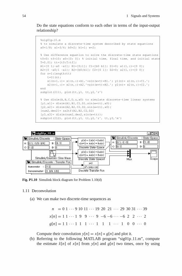
54 1 Signals and Systems
Do the state equations conform to each other in terms of the input-outputrelationship?
%sig01p 10.m% to simulate a discrete-time system described by state equationsa0=1/8; a1=3/4; b0=2; b1=1; w=2;
% Use difference equation to solve the discrete-time state equationst0=0; tf=10; x0=[0; 0]; % initial time, final time, and initial stateT=0.01; tt=[t0:T:tf];A1=[0 1;-a0 -a1]; B1=[0;1]; C1=[b0 b1]; D1=0; x1(1,:)=[0 0];A2=[0 -a0;1 -a1]; B2=[b0;b1]; C2=[0 1]; D2=0; x2(1,:)=[0 0];for n=1:length(tt)
t=tt(n);x1(n+1,:)= x1(n,:)*A1.’+sin(w*t)*B1.’; y1(n)= x1(n,:)*C1.’;x2(n+1,:)= x2(n,:)*A2.’+sin(w*t)*B2.’; y2(n)= x2(n,:)*C2.’;
endsubplot(211), plot(tt,y1, tt,y2,’r’)
% Use dlsim(A,B,C,D,u,x0) to simulate discrete-time linear systems[y1,x1]= dlsim(A1,B1,C1,D1,sin(w*tt),x0);[y2,x2]= dlsim(A2,B2,C2,D2,sin(w*tt),x0);[num2,den2]= ss2tf(A2,B2,C2,D2)[y3,x3]= dlsim(num2,den2,sin(w*tt));subplot(212), plot(tt,y1, tt,y2,’r’, tt,y3,’m’)
Fig. P1.10 Simulink block diagram for Problem 1.10(d)
1.11 Deconvolution
(a) We can make two discrete-time sequences as
n = 0 1 · · · 9 10 11 · · · 19 20 21 · · · 29 30 31 · · · 39
x[n] = 1 1 · · · 1 9 9 · · · 9 −6 −6 · · · −6 2 2 · · · 2
g[n] = 1 1 · · · 1 1 1 · · · 1 1 1 · · · 1 0 0 · · · 0
Compute their convolution y[n] = x[n] ∗ g[n] and plot it.(b) Referring to the following MATLAB program “sig01p 11.m”, compute
the estimate x[n] of x[n] from y[n] and g[n] two times, once by using

Problems 55
Eq. (1.4.5) and once by using Eq. (1.4.7). Compare the two results in termsof how close they are to the original input sequence x[n].
%sig01p 11.mclear, clfx=[ones(1,30) zeros(1,10)]; Nx=length(x);g=ones(10,1)*[1 9 -6 2]; g=g(:).’; Ng=length(g);n=0:Nx+Ng-2;y=conv(x,g);subplot(313), stem(n,y,’.’)% Deconvolutionfor m=1:Ng
for n=1:m, G(m,n)=g(m-n+1); end % Eq.(1.4.5)endx0=(Gˆ-1*y(1:Ng)’)’;x1(1)=y(1)/g(1);for n=2:Nx
x1(n)=y(n);for m=1:n-1, x1(n)=x1(n)-g(n-m+1)*x1(m); end % Eq.(1.4.7)x1(n)=x1(n)/g(1);
enderr0=norm(x0-x)err1=norm(x1-x)
(cf.) Another way to compute deconvolution is to use the MATLAB commandx=deconv(y,g).
1.12 Correlation and Matched Filter for Signal DetectionConsider Example 1.5 and the related program “sig01e05.m” again.
(a) To see the transmitted signal x, insert the following statement and run theprogram to check if you can get the results as depicted in Fig. 1.21(c), (d1),and (d2).
subplot(311), plot(tt,xbuffer)
(b) Remove the zero periods between the signals in the input. Can you stillnotice the corresponding signal arrival times from (local) maxima of theoutput of each matched filter? To simulate this situation, modify the state-ment for generating the transmitted signal as follows:
x= [x1 x2 x1 x2 x2];
(c) If we sample the matched filter outputs every 2 s, can we use the sampledoutput to detect the signal successfully based on which filter output is themaximum? To simulate this situation, insert the following statements intothe last part of the for loop:
if mod(n,Nx)==0fprintf(’At t=%5.2f, Matched filter output=%5.2f %5.2f\n’, n*Ts,y);
end

56 1 Signals and Systems
(d) If the input is contaminated with a Gaussian noise with zero mean andvariance of σ 2 = 0.32, will the detection performance be harmed severely?To simulate this situation, modify one of the statements in the for loop asfollows:
xbuffer= [x(n)+0.3*randn xbuffer(1:end-1)];
(cf.) The system with impulse response gi (t) = xi (T − t) is called the‘matched filter’ for the signal xi (t) because it is tuned to xi (t) so thatit can produce the maximum output to the input xi (t).
1.13 Walsh Functions [W-3] and Matched Filter
0
(a)
0
1
1 1.5 2t
–1
(b)
00
–1
1
1 2t
(c)
0
–1
1
0 1 2 t
(d)
0
–1
1
0 1 2t
Fig. P1.13
With the program “sig01e05.m” modified in Problem 1.12, answer thefollowing questions.
(a) If we use the signal waveform of Fig. P1.13(a) in place of that of Fig. 1.21(a1),how are the matched filter outputs sampled every 2 s changed? Can youexplain why the output of a matched filter is not close to zero 2 s afteranother signal arrives in contrast with the case where the signal waveformsof Fig. 1.21(a1) and (b1) are used?
(cf.) This gives us a chance to think about how we can design the signalwaveforms in such a way the difference between the (sampled) out-put of a matched filter to the input for which it is tuned and the (sam-pled) output to other input signals can be maximized, for the purposeof minimizing the suffer from possible noise/distortion/interferencein a communication system. It is desirable to have the signal wave-forms orthogonal to each other so that the integrations of theirproducts are zero.
(b) Consider the three signal waveforms x1(t), x2(t), and x3(t) of duration T =2 [s], known as Walsh functions, which are depicted in Fig. P1.13(b), (c),and (d) and represent a, b, and c, respectively.
- Are the three signals orthonormal in the following sense?
∫ T
0xi (t)x j (t)dt = δ[i − j] =
{1 for i = j
0 for i �= j(P1.13.1)

Problems 57
- Modify the program “sig01e05.m” to simulate the situation that thefollowing input signal is applied to the three matched filters with theimpulse response gi (t) = xi (T − t):
x(t) = [x1(t) x2(t − T ) x3(t − 2T ) x2(t − 3T ) x1(t − 4T )] (P1.13.2)
Does the receiver detect the received signals successfully from the sam-pled outputs of the matched filters for all the zero-mean Gaussian noiseof variance σ 2 = 0.32?
1.14 Correlation Function and Radar (Radio Detection and Ranging) System(Problem 3.28(e) of [O-1])A radar transmits a short pulse of radio signal (electromagnetic radiation) andmeasures the time it takes for the reflection to return from the target. Thedistance is one-half the product of the round trip time and the speed of thesignal [W-1].
0 00
1
–1
t t
p1(t ) p2(t )
(a) (b)
0
1
–1
Fig. P1.14
(a) Let the transmitted pulse be p(t) and the received pulse a p(t − t1) where t1is the round trip time. Show that their crosscorrelation φxp(t) is maximizedat t = t1:
φxp(t1) = Maxt
φxp(t) (P1.14.1)
where
φxp(t) =∫
x(t + τ )p(τ )dτ = a∫
p(t − t1 + τ )p(τ )dτ (P1.14.2)
<Hint> To find the time at which the crosscorrelation is maximized, usethe Cauchy-Schwartz inequality:
∫ b
au(τ )v(τ )dτ ≤
(∫ b
au2(τ )dτ
)1/2 (∫ b
av2(τ )dτ
)1/2
(P1.14.3)
where the equality holds if and only if u(τ ) = v(τ ).(b) Since the radar looks for the peak of the correlation function to find the
arrival time of returning signal, it would be good to use a pulse signal

58 1 Signals and Systems
(One OFDM symbol duration)
N_FFTN_SD
N_GI
Prefix
(1) win_sig[n] = r[n](2) win_power[n] = r2[n]
(4) win_corr[n] = win_sig[n] win_sig[n–N_FFT]
(5) windowed_corr =
win_power[m](3) win_energy[n] =
correlation[n] = Windowed_corr
m=n-N_Gl+1
m=n-N_Gl+1
r [n]. ..
. ..
. ..
nwin_corr[m]
win_energy[n] win_energy[n–N_FFT]
∑
n∑
. ..
√
⎧⎩ ⎧⎩
Fig. P1.15 Windows to detect an OFDM symbol using correlation
p(t) that has a sharply peaked autocorrelation function against possibledistortion in the returning signal. Which of the two pulses in Fig. P1.14 isbetter?
1.15 OFDM Symbol Timing Using CorrelationSuppose an OFDM (Orthogonal Frequency Division Multiplexing) commu-nication system in which an OFDM symbol consists of N FFT (Fast FourierTransform) points and N GI = 16 prefix points where the cyclic prefix is arepeat of the end of the symbol at the beginning. Let us consider a problemof detecting the start time of each OFDM symbol by using the correlationbetween the prefix and the end part of the symbol. Since we cannot storeuncountably many samples of the received signal r[n], we use several win-dows (buffers) to store some duration of signal samples, powers, energies, andcorrelations as shown in Fig. P1.15 where the contents of each window is asfollows:
(1) win sig[n] = r[n] with the size of at least N FFT + 1(2) win power[n] = r[n]2 with the size of N GI + 1(3) win energy[n] = ∑n
m=n−N GI+1 win power[m] with the size of N FFT + 1(4) win corr[n] = r[n]r[n − N FFT] with the size of N GI + 1
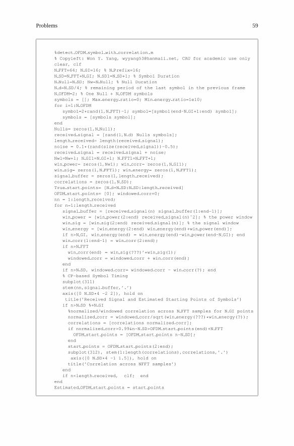
Problems 59
%detect OFDM symbol with correlation.m% Copyleft: Won Y. Yang, [email protected], CAU for academic use onlyclear, clfN FFT=64; N GI=16; % N Prefix=16;N SD=N FFT+N GI; N SD1=N SD+1; % Symbol DurationN Null=N SD; Nw=N Null; % Null DurationN d=N SD/4; % remaining period of the last symbol in the previous frameN OFDM=2; % One Null + N OFDM symbolssymbols = []; Max energy ratio=0; Min energy ratio=1e10;for i=1:N OFDM
symbol=2*rand(1,N FFT)-1; symbol=[symbol(end-N GI+1:end) symbol];symbols = [symbols symbol];
endNulls= zeros(1,N Null);received signal = [rand(1,N d) Nulls symbols];length received= length(received signal);noise = 0.1*(rand(size(received signal))-0.5);received signal = received signal + noise;Nw1=Nw+1; N GI1=N GI+1; N FFT1=N FFT+1;win power= zeros(1,Nw1); win corr= zeros(1,N GI1);win sig= zeros(1,N FFT1); win energy= zeros(1,N FFT1);signal buffer = zeros(1,length received);correlations = zeros(1,N SD);True start points= [N d+N SD:N SD:length received]OFDM start points= [0]; windowed corr=0;nn = 1:length received;for n=1:length received
signal buffer = [received signal(n) signal buffer(1:end-1)];win power = [win power(2:end) received signal(n)ˆ2]; % the power windowwin sig = [win sig(2:end) received signal(n)]; % the signal windowwin energy = [win energy(2:end) win energy(end)+win power(end)];if n>N GI, win energy(end) = win energy(end)-win power(end-N GI); endwin corr(1:end-1) = win corr(2:end);if n>N FFTwin corr(end) = win sig(???)’*win sig(1);windowed corr = windowed corr + win corr(end);
endif n>N SD, windowed corr= windowed corr - win corr(?); end% CP-based Symbol Timingsubplot(311)stem(nn,signal buffer,’.’)axis([0 N SD*4 -2 2]), hold ontitle(’Received Signal and Estimated Starting Points of Symbols’)if n>N SD %+N GI
%normalized/windowed correlation across N FFT samples for N GI pointsnormalized corr = windowed corr/sqrt(win energy(???)*win energy(?));correlations = [correlations normalized corr];if normalized corr>0.99&n-N SD>OFDM start points(end)+N FFT
OFDM start points = [OFDM start points n-N SD];endstart points = OFDM start points(2:end);subplot(312), stem(1:length(correlations),correlations,’.’)axis([0 N SD*4 -1 1.5]), hold on
title(’Correlation across NFFT samples’)endif n<length received, clf; end
endEstimated OFDM start points = start points

60 1 Signals and Systems
At each iteration when a sampled signal arrives, we compute the normalizedand windowed correlation
correlation[n] = windowed corr[n]√win energy[n]win energy[n − N FFT]
?> Threshold(0.99)
(P1.15.1)
with windowed corr[n] =∑n
m=n−N GI+1win corr[m]
to determine whether the current sample is the end of an OFDM symbol ornot. If the normalized correlation is found to exceed the threshold value, say,0.99, we set the start time of the detected symbol to N SD (one OFDM sym-bol duration) samples before the detection time. Complete the above program“detect OFDM symbol with correlation.m” so that it implements this OFDMsymbol timing scheme. Also run it to check if it works.

Chapter 2Continuous-Time Fourier Analysis
Contents
2.1 Continuous-Time Fourier Series (CTFS) of Periodic Signals . . . . . . . . . . . . . . . . . . . . . . 622.1.1 Definition and Convergence Conditions
of CTFS Representation . . . . . . . . . . . . . . . . . . . . . . . . . . . . . . . . . . . . . . . . . . . . . 622.1.2 Examples of CTFS Representation . . . . . . . . . . . . . . . . . . . . . . . . . . . . . . . . . . . . 652.1.3 Physical Meaning of CTFS Coefficients – Spectrum . . . . . . . . . . . . . . . . . . . . . . 70
2.2 Continuous-Time Fourier Transform of Aperiodic Signals . . . . . . . . . . . . . . . . . . . . . . . . 732.3 (Generalized) Fourier Transform of Periodic Signals . . . . . . . . . . . . . . . . . . . . . . . . . . . . . 772.4 Examples of the Continuous-Time Fourier Transform . . . . . . . . . . . . . . . . . . . . . . . . . . . . 782.5 Properties of the Continuous-Time Fourier Transform . . . . . . . . . . . . . . . . . . . . . . . . . . . . 86
2.5.1 Linearity . . . . . . . . . . . . . . . . . . . . . . . . . . . . . . . . . . . . . . . . . . . . . . . . . . . . . . . . . . 862.5.2 (Conjugate) Symmetry . . . . . . . . . . . . . . . . . . . . . . . . . . . . . . . . . . . . . . . . . . . . . . . 862.5.3 Time/Frequency Shifting (Real/Complex Translation) . . . . . . . . . . . . . . . . . . . . 882.5.4 Duality . . . . . . . . . . . . . . . . . . . . . . . . . . . . . . . . . . . . . . . . . . . . . . . . . . . . . . . . . . . . 882.5.5 Real Convolution . . . . . . . . . . . . . . . . . . . . . . . . . . . . . . . . . . . . . . . . . . . . . . . . . . . 892.5.6 Complex Convolution (Modulation/Windowing) . . . . . . . . . . . . . . . . . . . . . . . . . 902.5.7 Time Differential/Integration – Frequency Multiplication/Division . . . . . . . . . . 942.5.8 Frequency Differentiation – Time Multiplication . . . . . . . . . . . . . . . . . . . . . . . . . 952.5.9 Time and Frequency Scaling . . . . . . . . . . . . . . . . . . . . . . . . . . . . . . . . . . . . . . . . . . 952.5.10 Parseval’s Relation (Rayleigh Theorem) . . . . . . . . . . . . . . . . . . . . . . . . . . . . . . . . 96
2.6 Polar Representation and Graphical Plot of CTFT . . . . . . . . . . . . . . . . . . . . . . . . . . . . . . . 962.6.1 Linear Phase . . . . . . . . . . . . . . . . . . . . . . . . . . . . . . . . . . . . . . . . . . . . . . . . . . . . . . . 972.6.2 Bode Plot . . . . . . . . . . . . . . . . . . . . . . . . . . . . . . . . . . . . . . . . . . . . . . . . . . . . . . . . . . 97
2.7 Summary . . . . . . . . . . . . . . . . . . . . . . . . . . . . . . . . . . . . . . . . . . . . . . . . . . . . . . . . . . . . . . . . . 98Problems . . . . . . . . . . . . . . . . . . . . . . . . . . . . . . . . . . . . . . . . . . . . . . . . . . . . . . . . . . . . . . . . . 99
Since the great contribution and revolutionary discovery of Jean Baptiste JosephFourier saw the light in 1822 after passing through the long dark tunnel of J.L.Lagrange’s stubborn objection and was supported by P.L. Dirichlet’s rigorous math-ematical proof in 1829, the Fourier series and transform techniques have played verysignificant role in so many disciplines within the fields of mathematics, science, andengineering.
Joseph Fourier (1768∼1830) was a French mathematician and physicist who ini-tiated the investigation of Fourier series and its application. Born as a son of a tailor,he was orphaned at age 8. In 1784, at only 16 years of age, he became a mathematicsteacher at the Ecole Royale Militaire of Auxerre, debarred from entering the army
W.Y. Yang et al., Signals and Systems with MATLAB R©,DOI 10.1007/978-3-540-92954-3 2, C© Springer-Verlag Berlin Heidelberg 2009
61

62 2 Continuous-Time Fourier Analysis
on account of his obscurity and poverty. In 1795, Fourier took a faculty positionat the Ecole Normale (Polytechnique) in Paris, which is an elite institution train-ing high school teachers, university professors, and researchers. In 1798, he joinedNapoleon’s army in its expedition to Egypt as scientific advisor to help establisheducational facilities there and carry out archaeological explorations.
Eluding the Nelson’s British fleet, the Napoleon’s Egyption expedition fleet of300 ships, 30,000 infantry, 2,800 cavalry, and 1,000 cannons started Toulon onMay 19,1798, sailing for Alexandria. The great expedition plan plotted by Napoleonattached a library with lots of books, many measurement instruments, various lab-oratory apparatuses, and about 500 civilians to the army; 150 of them were artists,scientists, scholars, engineers, and technicians. These human and physical resourcesformed the Institut d‘Egypte in Cairo after Egypt was conquered by Napoleon.Napoleon Bonaparte (1769∼1821) not yet 30 years old, a great hero in the humanhistory, and Joseph Fourier, a great scholar of about the same age in their youth wereon board the flagship L’Orient of the expedition fleet. What were they thinking ofwhen walking around on the deck and looking up the stars twinkling in the sky abovethe Mediterranean Sea at several nights in May of 1798? One might have dreamedof Julius Caesar, who conquered Egypt about 1,800 years ago, falling in love withthe Queen Cleopatra, or might have paid a tribute to the monumental achievementsof the great king Alexander, who conquered one third of the earth, opening the roadbetween the West and the Orient. The other might have refreshed his memory onwhat he wrote in his diary on his 21st birthday, Yesterday was my 21st birthday,at that age Newton and Pascal had already acquired many claims to immortality,arranging his ideas on Fourier series and heat diffusion or recollecting his politicalideology which had swept him and made him get very close to guillotine in thevortex of French Revolution.
2.1 Continuous-Time Fourier Series (CTFS)of Periodic Signals
2.1.1 Definition and Convergence Conditionsof CTFS Representation
Let a function x(t) be periodic with period P in t , that is,
x(t) = x(t + P) ∀ t (2.1.1)
where P [s] and ω0 = 2π/P [rad/s] are referred to as the fundamental periodand fundamental (angular) frequency, respectively, if P is the smallest positive realnumber to satisfy Eq. (2.1.1) for periodicity. Suppose x(t) satisfies at least one ofthe following conditions A and B:

2.1 Continuous-Time Fourier Series (CTFS) of Periodic Signals 63
< Condition A >
(A1) The periodic function x(t) is square-integrable over the period P , i.e.,∫P
|x(t)|2 dt < ∞ (2.1.2a)
where∫
P means the integration over any interval of length P . This impliesthat the signal described by x(t) has finite power.
< Condition B : Dirichlet condition >
(B1) The periodic function x(t) has only a finite number of extrema and disconti-nuities in any one period.
(B2) These extrema are finite.(B3) The periodic function x(t) is absolutely-integrable over the period P , i.e.,∫
P|x(t)| dt < ∞ (2.1.2b)
Then the periodic function x(t) can be represented by the following forms ofcontinuous-time Fourier series (CTFS), each of which is called the Fourier seriesrepresentation:<Trigonometric form>
x(t) = a0 +∑∞
k=1ak cos kω0t +
∑∞k=1
bk sin kω0t (2.1.3a)
with ω0 = 2π
P(P : the period of x(t))
where the Fourier coefficients a0, ak , and bk are
a0 = 1
P
∫P
x(t) dt (the integral over one period P)
ak = 2
P
∫P
x(t) cos kω0t dt (2.1.3b)
bk = 2
P
∫P
x(t) sin kω0t dt
<Magnitude-and-Phase form>
x(t) = d0 +∑∞
k=1dk cos(kω0t + φk) (2.1.4a)
where the Fourier coefficients are
d0 = a0, dk =√
a2k + b2
k , φk = tan−1(−bk/ak) (2.1.4b)

64 2 Continuous-Time Fourier Analysis
<Complex Exponential form>
x(t) = 1
P
∑∞k=−∞ ck e jkω0t (2.1.5a)
where the Fourier coefficients are
ck =∫
Px(t) e− jkω0t dt (the integral over one period P) (2.1.5b)
Here, the k th frequency kω0 (|k| > 1) with fundamental frequency ω0 = 2π/P =2π f0 [rad/s](P: period) is referred to as the k th harmonic. The above three forms ofFourier series representation are equivalent and their Fourier coefficients are relatedwith each other as follows:
c0 =∫
Px(t) dt = Pd0 = Pa0 (2.1.6a)
ck =∫
Px(t) e− jkω0t dt =
∫P
x(t) (cos kω0t − j sin kω0t) dt
= P
2(ak − jbk) = P
2dk∠φk (2.1.6b)
c−k =∫
Px(t) e jkω0t dt =
∫P
x(t) (cos kω0t + j sin kω0t) dt
= P
2(ak + jbk) = P
2dk∠ − φk = c∗
k (2.1.6c)
a0 = c0
P, ak = ck + c−k
P= 2Re{ck}
P, bk = c−k − ck
j P= −2Im{ck}
P(2.1.6d)
The plot of Fourier coefficients (2.1.4b) or (2.1.5b) against frequency kω0 is referredto as the spectrum. It can be used to describe the spectral contents of a signal,i.e., depict what frequency components are contained in the signal and how theyare distributed over the low/medium/high frequency range. We will mainly useEqs. (2.1.5a) and (2.1.5b) for spectral analysis.
<Proof of the Complex Exponential Fourier Analysis Formula (2.1.5b)>To show the validity of Eq. (2.1.5b), we substitute the Fourier synthesis formula(2.1.5a) with the (dummy) summation index k replaced by n into Eq. (2.1.5b) as
ck?=∫
P
1
P
∑∞n=−∞ cn e jnω0t e− jkω0t dt =
∑∞n=−∞ cn
1
P
∫P
e j(n−k) 2πP t dt
O.K.= ck
(2.1.7)

2.1 Continuous-Time Fourier Series (CTFS) of Periodic Signals 65
This equality holds since
1
P
∫ P/2
−P/2e j(n−k) 2π
P t dt
=
⎧⎪⎪⎨⎪⎪⎩
1P· j(n−k)2π/P e j(n−k) 2π
P t∣∣∣P/2
−P/2= 0 for n �= k
1P
∫ P/2−P/2 dt = 1 for n = k
= δ[n − k] (2.1.8)
2.1.2 Examples of CTFS Representation
Example 2.1 Fourier Spectra of a Rectangular (Square) Wave and a TriangularWave
(a) CTFS Spectrum of a Rectangular (Square) Wave (Fig. 2.1(a1))Consider an even rectangular wave x(t) with height A, duration D, andperiod P:
x(t) = A rD/P (t) (E2.1.1)
where rD/P (t) ={
1 for |t − m P| ≤ D/2(m : an integer)
0 elsewhere
A
A
(a1) A rectangular wave ArD/P (t ): even∼
(b1) A triangular wave AλD/P (t ): even∼
(b2) A triangular wave AλD/P (t–D): odd∼
(a2) A rectangular wave ArD/P (t–D/2 ): odd∼
–P
–P
P
P
t–D/2 0 D/2 –P
t–D 0 D
t
P
A
A
P2Dt
–2D–P 0–D 0 D
Fig. 2.1 Rectangular waves and triangular waves

66 2 Continuous-Time Fourier Analysis
We use Eq. (2.1.5b) to obtain the Fourier coefficients as
ck =∫ P/2
−P/2A rD/P (t) e− jkω0t dt = A
∫ D/2
−D/2e− jkω0t dt = A
− jkω0e− jkω0t
∣∣∣∣D/2
−D/2
= Ae jkω0 D/2 − e− jkω0 D/2
jkω0= AD
sin(kω0 D/2)
kω0 D/2
= AD sinc
(k
D
P
)with ω0 = 2π
P(E2.1.2)
Now we can use Eq. (2.1.5a) to write the Fourier series representation of therectangular wave as
ArD/P (t)(2.1.5a)= 1
P
∑∞k=−∞ AD sinc
(k
D
P
)e jkω0t
= AD
P+∑∞
k=1
2AD
P
sin(kπ D/P)
kπ D/Pcos kω0t (E2.1.3)
In the case of D = 1 and P = 2D = 2 as depicted in Fig. 2.2(a1), the(magnitude) spectrum is plotted in Fig. 2.2(b1).(Q) What about the case of P = D, which corresponds to a constant DC (DirectCurrent) signal?
A = 1
ck
ck
–4 –4 –2 0 2 4
= 2π
6 8–6–8
00
1
–2
(a1) A rectangular wave (b1) The magnitude spectrum
2 t k
k
P
P
D
D
ω0P
ω0
40
A = 1
–4
0
–2
(a2) A triangular wave
2 t 40 –4 –2 0 2 4
= 2π
6 8–6–80
1
(b2) The magnitude spectrum
ω0P
ω0
Fig. 2.2 Rectangular/triangular waves and their CTFS magnitude spectra

2.1 Continuous-Time Fourier Series (CTFS) of Periodic Signals 67
(b) CTFS Spectrum of a Triangular Wave (Fig. 2.1(b1))Consider an even triangular wave x(t) with maximum height A, duration 2D,and period P:
x(t) = AλD/P (t) (E2.1.4)
where λ D/P (t) ={
1 − t/D for |t − m P| ≤ D (m : an integer)
0 elsewhere
We use Eq. (2.1.5b) to obtain the Fourier coefficients as
ck =∫ P/2
−P/2A
(1 − |t |
D
)e− jkω0t dt =
∫ D
−DA
(1 − |t |
D
)cos(kω0t) dt
= 2∫ D
0A
(1 − t
D
)cos(kω0t) dt = 2A
(1 − t
D
)1
kω0sin(kω0t)
∣∣∣∣D
0
−∫ D
02A
(− 1
D
)1
kω0sin(kω0t) dt = −2A
1
(kω0)2 Dcos(kω0t)
∣∣∣∣D
0
= 2AD1 − cos(kω0 D)
(kω0 D)2= AD
4 sin2(kω0 D/2)
(kω0 D/2)2
= AD sin c2
(k
D
P
)with ω0 = 2π
P(E2.1.5)
Now we can use Eq. (2.1.5a) to write the Fourier series representation of thetriangular wave as
AλD/P (t)(2.1.5a)= 1
P
∑∞k=−∞ AD sinc2
(k
D
P
)e jkω0t (E2.1.6)
In the case of D = 1 and P = 2D = 2 as depicted in Fig. 2.2(a2), thecorresponding (magnitude) spectrum is plotted in Fig. 2.2(b2).
(c) MATLAB program to get the Fourier spectraOnce you have defined and saved a periodic function as an M-file, you can usethe MATLAB routine “CTFS exponential ()” to find its complex exponentialFourier series coefficients (ck’s). Interested readers are invited to run the follow-ing program “cir02e01.m” to get the Fourier coefficients and plot the spectra fora rectangular wave and a triangular wave as in Fig. 2.2.

68 2 Continuous-Time Fourier Analysis
%sig02e01.m : plot Fig. 2.2 (CTFS spectra of rectangular/triangular wavesclear, clfglobal P DN=8; k= -N:N; % the range of frequency indicesfor i=1:2
if i==1 % true Fourier series coefficients for a rectangular wavex = ’rectangular wave’; P=2; D=1; c true= D*sinc(k*D/P);else % true Fourier series coefficients for a triangular wavex = ’triangular wave’; P=2; D=1; c true= D*sinc(k*D/P).ˆ2;
endw0=2*pi/P; % fundamental frequencytt=[-400:400]*P/200; % time interval
xt = feval(x,tt); % original signal[c,kk] = CTFS exponential(x,P,N);[c; c true] % to compare with true Fourier series coefficientsdiscrepancy between numeric and analytic=norm(c-c true)jkw0t= j*kk.’*w0*tt;xht = real(c/P*exp(jkw0t)); % Eq. (2.1.5a)
subplot(219+i*2), plot(tt,xt,’k-’, tt,xht,’b:’)axis([tt(1) tt(end) -0.2 1.2]), title(’Periodic function x(t)’)c mag = abs(c); c phase = angle(c);subplot(220+i*2), stem(kk, c mag), title(’CTFS Spectrum |X(k)|’)
end
function y=rectangular wave(t)global P Dtmp=min(abs(mod(t,P)),abs(mod(-t,P))); y= (tmp<=D/2);
function y=triangular wave(t)global P Dtmp= min(abs(mod(t,P)),abs(mod(-t,P))); y=(tmp<=D).*(1-tmp/D);
function [c,kk]=CTFS exponential(x,P,N)% Find the complex exponential Fourier coefficients c(k) for k=-N:N% x: A periodic function with period P% P: Period, N: Maximum frequency index to specify the frequency rangew0=2*pi/P; % the fundamental frequency [rad/s]xexp jkw0t = [x ’(t).*exp(-j*k*w0*t)’];xexp jkw0t= inline(xexpjkw0t ,’t’,’k’,’w0’);kk=-N:N; tol=1e-6; % the frequency range tolerance on numerical errorfor k=kk
c(k+N+1)= quadl(xexp jkw0t,-P/2,P/2,tol,[],k,w0); % Eq. (2.1.5b)end
%sig02 01.m : plot Fig. 2.3 (CTFS reconstruction)clear, clfglobal P DP=2; w0=2*pi/P; D=1; % period, fundamental frequency, and durationtt=[-400:400]*P/400; % time interval of 4 periodsx = ’rectangular wave’;xt = feval(x,tt); % original signalplot(tt,xt,’k:’), hold onNs= [1 3 9 19];for N=Ns
k= -N:N; jkw0t= j*k.’*w0*tt; % the set of Fourier reconstruction termsc= D*sinc(k*D/P);xht = real(c/P*exp(jkw0t)); % Eq. (2.1.9)plot(tt,xht,’b’), hold on, pause
endaxis([tt(1) tt(end) -0.2 1.2])

2.1 Continuous-Time Fourier Series (CTFS) of Periodic Signals 69
1
0.5
0
–2 –1
x (t ) = e = –N
N = 1 N = 3 N = 9
N = 19
N jkω0tc
k k1P
∑∧
0 1 2
Fig. 2.3 Examples of the approximate Fourier reconstruction for a rectangular pulse
At this point, you may wonder how a rectangular wave with discontinuities canbe represented by the sum of trigonometric or complex exponential functions thatare continuous for all t . To satisfy your curiosity, let us consider the approximateFourier series reconstruction formula.
xN (t) = 1
P
∑N
k=−Nck e jkω0t (2.1.9)
This can be used to reconstruct the original time function x(t) from its Fourierseries coefficients. We can use the above MATLAB program ‘sig02 01.m’ to plotthe Fourier series reconstructions of a rectangular wave with increasing number ofterms N = 1, 3, 9, 19,. . . as in Fig. 2.3.
The following remark with Fig. 2.3 will satisfy your curiosity:
Remark 2.1 Convergence of Fourier Series Reconstruction
(1) The Fourier series convergence condition A stated in Sect. 2.1.1 guarantees thatthe Fourier coefficients are finite and the Fourier series reconstruction xN (t)converges to the original time function x(t) in the sense that
∫P
|xN (t) − x(t)|2 dt → 0 as N → ∞
(2) The Fourier series convergence condition B stated in Sect. 2.1.1 guarantees thefollowing:
- The Fourier coefficients are finite.- The Fourier series reconstruction xN (t) converges to the original time func-
tion x(t) at every t except the discontinuities of x(t) and to the average valueof the limits from the left/right at each discontinuity.
(3) Figure 2.3 illustrates that xN (t) has ripples around the discontinuities of x(t),whose magnitude does not decrease as N → ∞. This is called the Gibbsphenomenon.
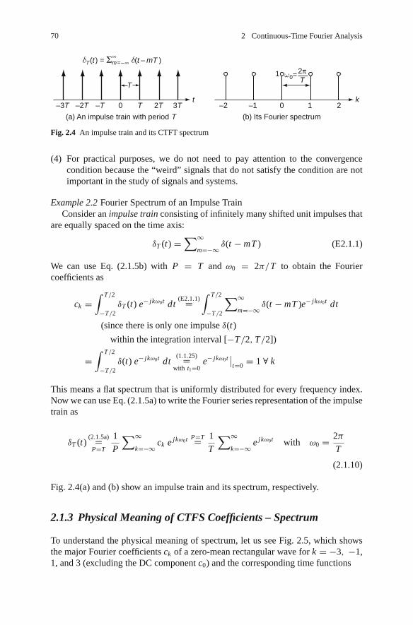
70 2 Continuous-Time Fourier Analysis
(a) An impulse train with period T
–3T –2T –T 0 T 2T
T
3T –2 –1 0 1
1
2kt
(b) Its Fourier spectrum
ω 0=2πT
δT(t ) = Σm=–∞ δ(t – mT )∞
Fig. 2.4 An impulse train and its CTFT spectrum
(4) For practical purposes, we do not need to pay attention to the convergencecondition because the “weird” signals that do not satisfy the condition are notimportant in the study of signals and systems.
Example 2.2 Fourier Spectrum of an Impulse TrainConsider an impulse train consisting of infinitely many shifted unit impulses that
are equally spaced on the time axis:
δT (t) =∑∞
m=−∞ δ(t − mT ) (E2.1.1)
We can use Eq. (2.1.5b) with P = T and ω0 = 2π/T to obtain the Fouriercoefficients as
ck =∫ T/2
−T/2δT (t) e− jkω0t dt
(E2.1.1)=∫ T/2
−T/2
∑∞m=−∞ δ(t − mT )e− jkω0t dt
(since there is only one impulse δ(t)
within the integration interval [−T/2, T/2])
=∫ T/2
−T/2δ(t) e− jkω0t dt
(1.1.25)=with t1=0
e− jkω0t∣∣t=0 = 1 ∀ k
This means a flat spectrum that is uniformly distributed for every frequency index.Now we can use Eq. (2.1.5a) to write the Fourier series representation of the impulsetrain as
δT (t)(2.1.5a)=
P=T
1
P
∑∞k=−∞ ck e jkω0t P=T= 1
T
∑∞k=−∞ e jkω0t with ω0 = 2π
T
(2.1.10)
Fig. 2.4(a) and (b) show an impulse train and its spectrum, respectively.
2.1.3 Physical Meaning of CTFS Coefficients – Spectrum
To understand the physical meaning of spectrum, let us see Fig. 2.5, which showsthe major Fourier coefficients ck of a zero-mean rectangular wave for k = −3, −1,1, and 3 (excluding the DC component c0) and the corresponding time functions

2.1 Continuous-Time Fourier Series (CTFS) of Periodic Signals 71
0
Re
Im0
C1
C3
C–1
C–3
P
P
P
P t
d3cos(3ω0t + φ3)
–3ω0 3ω0[rad/s]
–ω0[rad/s]ω0
d 3co
sφ3
d 1co
sφ1
φ3
φ1
d1cos(ω0t + φ1)d1cos(ω0t + φ1) + d3cos(3ω0t + φ3)
Fig. 2.5 Physical meaning of complex exponential Fourier series coefficients
1
P
(c−1 e− jω0t + c1 e jω0t
)and
1
P
(c−3 e− j3ω0t + c3 e j3ω0t
)The observation of Fig. 2.5 gives us the following interpretations of Fourierspectrum:
Remark 2.2 Physical Meaning of Complex Exponential Fourier Series Coefficients
(1) While the trigonometric or magnitude-and-phase form of Fourier series has onlynonnegative frequency components, the complex exponential Fourier series haspositive/negative frequency (±kω0) components that are conjugate-symmetricabout k = 0, i.e.,
ck(2.1.6b)= P
2dke jφk and c−k
(2.1.6c)= P
2dke− jφk → |c−k | = |ck | and φ−k = −φk
as shown in Sect. 2.1.1. This implies that the magnitude spectrum |ck | is (even)symmetric about the vertical axis k = 0 and the phase spectrum φk is oddsymmetric about the origin.
(2) As illustrated above, the k th component appears as the sum of the positive andnegative frequency components
ck
Pe jkω0t + c−k
Pe− jkω0t (2.1.6)= 1
2dke jφk e jkω0t + 1
2dke− jφk e− jkω0t
= dk cos(kω0t + φk)
which denote two vectors (phasors) revolving in the opposite direction withpositive (counter-clockwise) and negative (clockwise) angular velocities ±kω0
[rad/s] round the origin, respectively.(3) Figure 2.6 also shows that the spectrum presents the descriptive information of
a signal about its frequency components.
To get familiar with Fourier spectrum further, let us see and compare the spec-tra of the three signals, i.e., a rectangular wave, a triangular wave, and a constant

72 2 Continuous-Time Fourier Analysis
Magnitudespectrum
d1cos(ω0t +φ1) + d3cos(3ω0t +φ3)
d1cos(ω0t + φ1)
d3cos(3ω0t + φ3)
d1t
t
tfundamental component No 2nd harmonic
No dc componentTime
t
d1
d0 d2d3
kω0 kω0
0
Fr equenc y
d3
the 3rd harmonic component
Fig. 2.6 Physical meaning of spectrum – time domain vs. frequency domain
(DC: Direct Current) signal depicted in Fig. 2.7. The observations are stated in thefollowing remarks:
Remark 2.3 Effects of Smoothness and Period on Spectrum
(1) The smoother a time function is, the larger the relative magnitude of lowfrequency components to high frequency ones is. Compare Fig. 2.7(a1–b1),(a2–b2), and (a3–b3).
(cf.) The CTFS of the unit constant function can be obtained from Eq. (E2.1.3)with A = 1 and P = D.
P
D
D
–50
1
0
(a1) A rectangular wave with D = 1, P = 2 (b1) Its magnitude spectrum
(b2) Its magnitude spectrum
(b3) Its magnitude spectrum
(b4) Its magnitude spectrum
(a2) A triangular wave with D = 1, P = 2
(a3) A constant signal
(a4) A rectangular wave with D = 1, P = 4
5t –80
1
0 8k
P
D
–50
1
0 5t
–50
1
0 5t
–50
1
0 5t
ck = 2πω0
Pω0
= 2πP
ω0
ω0
–80
1
0 8k
ck
–80
1
0 8k
ck
–80
1
0 8k
ck
Fig. 2.7 The CTFS spectra of rectangular/triangular waves and a DC signal

2.2 Continuous-Time Fourier Transform of Aperiodic Signals 73
(2) The longer the period P is, the lower the fundamental frequency ω0 = 2π/Pbecomes and the denser the CTFS spectrum becomes. Compare Fig. 2.7(a4–b4)with (a1–b1).(cf.) This presages the continuous-time Fourier transform, which will be intro-
duced in the next section.
Now, let us see how the horizontal/vertical translations of a time function x(t)affect the Fourier coefficients.
<Effects of Vertical/Horizontal Translations of x(t) on the Fourier coefficients>Translating x(t) by ±A (+: upward, −: downward) along the vertical axis causesonly the change of Fourier coefficient d0 = a0 for k = 0 (DC component or averagevalue) by ±A. On the other side, translating x(t) along the horizontal (time) axis by±t1 (+: rightward, −: leftward) causes only the change of phases (φk’s) by ∓kω0t1,not affecting the magnitudes dk of Eq. (2.1.4b) or |ck | of Eq. (2.1.5b):
c′k
(2.1.5b)=∫
Px(t − t1) e− jkω0t dt =
∫P
x(t − t1) e− jkω0(t−t1+t1)dt
= e− jkω0t1
∫P
x(t − t1) e− jkω0(t−t1)dt(2.1.5b)= cke− jkω0t1 = |ck |∠(φk − kω0t1)
(2.1.11)
Note that x(t − t1) is obtained by translating x(t) by t1 in the positive (rightward)direction for t1 > 0 and by −t1 in the negative (leftward) direction for t1 < 0 alongthe horizontal (time) axis. Eq. (2.1.11) implies that horizontal shift of x(t) causes achange not in its magnitude spectrum but in its phase spectrum.
2.2 Continuous-Time Fourier Transform of Aperiodic Signals
In this section we will define the Fourier transform for aperiodic signals. Supposewe have an aperiodic signal x(t) of finite duration D > 0 and its periodic extensionxP (t) with period P > D that is obtained by repeating x(t) every P s.
Noting that, as we choose the period P to be longer, xP (t) appears to be identicalto x(t) over a longer interval, we can think of x(t) as the limit of xP (t) as P → ∞.Since xP (t) is periodic with period P , it can be represented by the Fourier series ofthe form
xP (t) = 1
P
∑∞k=−∞ ck e jkω0t = 1
2π
∑∞k=−∞ X ( jkω0) e jkω0tω0 with ω0 = 2π
P
where the CTFS coefficients are
X ( jkω0) = ck =∫
PxP (t) e− jkω0t dt =
∫ ∞
−∞x(t) e− jkω0t dt
Noting that xP (t) → x(t) and ω0 = 2π/P → 0 as P → ∞, we let ω0 = dω andkω0 = ω and take the limits of the above two equations as P → ∞ to write thecontinuous-time Fourier transform (CTFT) pair:

74 2 Continuous-Time Fourier Analysis
X ( jω) = F{x(t)} =∫ ∞
−∞x(t)e− jωt dt (Fourier transform/integral) (2.2.1a)
x(t) = F−1{X ( jω)} = 1
2π
∫ ∞
−∞X ( jω)e jωt dω (Inverse Fourier transform)
(2.2.1b)
where X ( jω), called the spectrum of x(t), has values at a continuum of frequenciesand is often written as X (ω) with the constant j omitted. Like the CTFS of periodicsignals, the CTFT of aperiodic signals provides us with the information concerningthe frequency contents of signals, while the concept of frequency describes ratherhow rapidly a signal changes than how fast it oscillates.
Note that the sufficient condition for the convergence of CTFT is obtained byreplacing the square-integrability condition (2.1.2a) of Condition A with
∫ ∞
−∞|x(t)|2 dt < ∞ (2.2.2a)
or by replacing the absolute-integrability condition (2.1.2b) of Condition B with
∫ ∞
−∞|x(t)| dt < ∞ (2.2.2b)
Remark 2.4 Physical Meaning of Fourier Transform – Signal Spectrum and Fre-quency Response
(1) If a time function x(t) represents a physical signal, its Fourier transformX ( jω) = F{x(t)} means the signal spectrum, which describes the frequencycontents of the signal.
(2) In particular, if a time function g(t) represents the impulse response of acontinuous-time LTI (linear time-invariant) system, its Fourier transformG( jω) = F{g(t)} means the frequency response, which describes how the sys-tem responds to a sinusoidal input of (angular) frequency ω (refer to Sect. 1.2.6for the definition of frequency response).
Remark 2.5 Frequency Response Existence Condition and Stability Condition ofa System
For the impulse response g(t) of a continuous-time LTI system, the absolute-integrability condition (2.2.2b) is identical with the stability condition (1.2.27a).This implies that a stable LTI system has a well-defined system function (frequencyresponse) G( jω) = F{g(t)}.Remark 2.6 Fourier Transform and Laplace Transform
For any square-integrable or absolutely-integrable causal function x(t) such thatx(t) = 0 ∀ t < 0, the Fourier transform can be obtained by substituting s = jω intothe Laplace transform:

2.2 Continuous-Time Fourier Transform of Aperiodic Signals 75
X ( jω)(2.2.1a)=
∫ ∞
−∞x(t)e− jωt dt
x(t)=0 for t<0=causal signal
∫ ∞
0x(t)e− jωt dt
(A.1)= X (s)|s= jω (2.2.3)
This argues that for a physical system having causal impulse response g(t), theFourier transform G( jω) of g(t), that is the frequency response, can be obtained bysubstituting s = jω into the system function G(s), which is the Laplace transformof g(t). (See Eq. (1.2.21).)
Example 2.3 CTFT Spectra of a Rectangular (Square) Pulse and a TriangularPulse
(a) CTFT Spectrum of a Rectangular (Square) Pulse (Fig. 2.8(a))Consider a single rectangular pulse with height 1 and duration D on the interval[−D/2, D/2]:
ArD(t) = A
(us
(t + D
2
)− us
(t − D
2
))={
A for − D/2 ≤ |t | < D/2
0 elsewhere(E2.3.1)
We use Eq. (2.2.1a) to obtain the CTFT coefficients as
1
Fourier transform
Fourier transformgeneralized
P = 4D
P = 2D
: PeriodFourier series ck Xkor
Fourier series
Fundamentalfrequency
–2π/D
–2π/D 2π/D
2πω0
ω0 PD
D
ω0
D
ω0
D
= :
2π/D00
–4 –40
t
t
–4 –4 –8
–16k
16
8k
0
0
0
0
–4 –40
t
t
X ( jω)D : Duration
(a) A rectangular pulse and its CTFT spectrum
(b) A rectangular wave and its CTFS spectrum
(d) A rectangular wave and its CTFT spectrum
(c) A rectangular wave and its CTFS spectrum
P
P
P = 2DP
⎥
⎥ ⎥ ⎥ ⎥
ck Xkor⎥ ⎥ ⎥ ⎥
⎥
⎥
X ( jω)⎥ ⎥
ω
ω
D
D
D
D
Fig. 2.8 The CTFT or CTFS spectra of rectangular pulses or waves

76 2 Continuous-Time Fourier Analysis
ARD( jω)(2.2.1a)=
∫ ∞
−∞ArD(t)e− jωt dt = A
∫ D/2
−D/2e− jωt dt = A
− jωe− jωt
∣∣∣∣D/2
−D/2
= Ae jωD/2 − e− jωD/2
jω= AD
sin(ωD/2)
ωD/2
= ADsinc
(ωD
2π
)(E2.3.2)
This CTFT spectrum is depicted in Fig. 2.8(a). The first zero crossing B =2π/D [rad/s] of the magnitude spectrum is often used as a measure of the fre-quency spread of a signal and called the zero-crossing (null-to-null) bandwidthof the signal.
(cf.) As a by-product, we can apply the inverse CTFT formula (2.2.1b) forEq. (E2.3.2) to get the integral of a sinc function:
rD(t)(2.2.1b)= 1
2π
∫ ∞
−∞RD( jω)e jωt dω
(E2.3.2)= 1
2π
∫ ∞
−∞D
sin(ωD/2)
ωD/2e jωt dω
us
(t + D
2
)− us
(t − D
2
)ω=2w= 1
π
∫ ∞
−∞
sin(wD)
we j2wt dw
Substituting t = 0 into this equation yields
1
π
∫ ∞
−∞
sin(wD)
wdw = us
(D
2
)− us
(− D
2
)= sign(D)=
⎧⎪⎨⎪⎩
1 for D > 0
0 for D = 0
−1 for D < 0
(E2.3.3)
(b) CTFT Spectrum of a Triangular PulseLike Eq. (E2.1.5), which is the CTFS coefficient of a triangular wave, we canfind the CTFT spectrum of a single triangular pulse x(t) = AλD(t) as
X ( jω) = AΛD ( jω) = ADsin2(ωD/2)
(ωD/2)2= AD sinc2
(ωD
2π
)(E2.3.4)
Figure 2.8(a) shows a rectangular pulse and its CTFT spectrum, while Fig. 2.8(b)and (c) show two rectangular waves and their CTFS spectra. These figures presentus an observation about the relationship between the CTFT of a single pulse x(t)and the CTFS of its periodic repetition xP (t) with period P , which is summarizedin the following remark.
Remark 2.7 Fourier Series and Fourier Transform
(1) We will mainly use the complex exponential Fourier coefficients, but seldomuse the trigonometric or magnitude-and-phase form of Fourier series. Thus,from now on, we denote the complex exponential Fourier coefficients of x(t)

2.3 (Generalized) Fourier Transform of Periodic Signals 77
by Xk instead of ck , which has been used so far to distinguish it from otherFourier coefficients ak, bk , or dk .
(2) As can be seen from comparing Eqs. (E2.1.2) and (E2.3.2) or (E2.1.5) and(E2.3.4), the relationship between the CTFT X ( jω) of x(t) and the CTFS coef-ficient Xk of xP (t) (the periodic extension of x(t) with period P) is as follows:
X ( jω)|ω=kω0=2πk/P = X ( jkω0) = Xk (2.2.4)
As the period P gets longer so that the fundamental frequency or frequencyspacing ω0=2π/P decreases, the Fourier coefficients Xk’s become more closelyspaced samples of the CTFT X ( jω), implying that the set of CTFS coefficientsapproaches the CTFT as P → ∞ (see Fig. 2.8(c), (b), and (a)).
(3) Unlike the discrete frequency kω0 of CTFS, the continuous frequency ω ofCTFT describes how abruptly the signal changes rather than how often itoscillates.
(4) If the CTFT of a single pulse x(t) and the CTFS of the periodic extension xP (t)were of different shape in spite of the same shape of x(t) and xP (t) over oneperiod P , it would be so confusing for one who wants the spectral informationabout a signal without knowing whether it is of finite duration or periodic. Inthis context, how lucky we are to have the same shape of spectrum (in the sensethat CTFS are just samples of CTFT) whether we take the CTFT of x(t) or theCTFS of xP (t)! Furthermore, you will be happier to see that even the CTFT ofxP (t) (Fig. 2.8(d)) is also of the same shape as the CTFS of xP (t), because onemight observe one period of xP (t) and mistake it for x(t) so that he or she wouldhappen to apply the CTFT for periodic signals. Are you puzzled at the CTFT ofa periodic signal? Then rush into the next section.
2.3 (Generalized) Fourier Transform of Periodic Signals
Since a periodic signal can satisfy neither the square-integrability condition (2.2.2a)nor the absolute-integrability condition (2.2.2b), the CTFTs of periodic signals arenot only singular but also difficult to compute directly. For example, let us try tocompute the CTFT of xk(t) = e jkω0t by using Eq. (2.2.1a):
F{xk(t)} (2.2.1a)=∫ ∞
−∞e jkω0t e− jωt dt =
∫ ∞
−∞e
− j(ω−kω0)tdt
(D.33)= 1
− j(ω − kω0)e
− j(ω−kω0)t∣∣∣T−T
∣∣∣∣T →∞
= 1
j(ω − kω0)
(e
j(ω−kω0)T − e− j(ω−kω0)T
)∣∣∣T =∞
=(
2 sin (ω − kω0)T
(ω − kω0)
)∣∣∣∣T =∞
=? (2.3.1)

78 2 Continuous-Time Fourier Analysis
To get around this mathematical difficulty, let us find the inverse CTFT of
Xk( jω) = 2π δ(ω − kω0)
by applying the inverse Fourier transform (2.2.1b):
F−1{Xk( jω)} (2.2.1b)= 1
2π
∫ ∞
−∞2π δ(ω − kω0)e jωt dω
(1.1.25)= ejkω0 t
This implies a CTFT pair as
xk(t) = ejkω0 t F↔ Xk( jω) = 2π δ(ω − kω0) (2.3.2)
Based on this relation, we get the Fourier transform of a periodic function x(t)from its Fourier series representation as follows:
x(t)(2.1.5a)= 1
P
∑∞k=−∞ Xk e jkω0t with ω0 = 2π
P
F↔ X ( jω)(2.3.2)= 2π
P
∑∞k=−∞ Xk δ(ω − kω0) (2.3.3)
This implies that the CTFT of a periodic signal consists of a train of impulseson the frequency axis having the same shape of envelope as the CTFS spectrum.Figure 2.8(d) is an illustration of Eq. (2.3.3) as stated in Remark 2.7(4).
Remark 2.8 Fourier Transform of a Periodic SignalIt would be cumbersome to directly find the CTFT of a periodic function. Thus wehad better find the CTFS coefficients first and then use Eq. (2.3.2) as illustrated inEq. (2.3.3).
2.4 Examples of the Continuous-Time Fourier Transform
Example 2.4 Fourier Transform of an Exponential FunctionFor an exponential function (Fig. 2.9(a)) with time constant T > 0
e1(t) = 1
Te−t/T us(t) with T > 0, (E2.4.1)
T : Time constant
B : Bandwidth
(a) A unilateral exponential signal (b) Its CTFT spectrum – magnitude
T1
0 0
1
1
T
Tt
B
E1( jω)
ωωc = 1/T
ωc =
e–11
e1(t ) = us(t )T
e–t /T 1
√2
T1 : Cutoff frequency
Fig. 2.9 A unilateral exponential signal and its CTFT spectrum
2.4 Examples of the Continuous-Time Fourier Transform 79
we have the Fourier transform
E1( jω) = F{e1(t)} (2.2.1a)=∫ ∞
−∞
1
Te−t/T us(t) e− jωt dt = 1
T
∫ ∞
0e−t/T e
− jωtdt
= 1
T
∫ ∞
0e
−(1/T + jω)tdt
(D.33)= − 1
T (1/T + jω)e
−(1/T + jω)t∣∣∣∞0
= 1
1 + jωT= 1√
1 + (ωT )2∠ − tan−1(ωT ) (E2.4.2)
whose magnitude is depicted in Fig. 2.9(b). From this magnitude spectrum, we seethat ωc = 1/T is the half-power frequency at which |E1( jω)| is 1/
√2 times the
maximum magnitude 1:
|E1( jω)| = 1√1 + (ω T )2
= 1√2
; 1 + (ω T )2 = 2; ωT = 1; ωc = 1
T(E2.4.3)
This example makes possible the following interpretations:
Remark 2.9 Signal Bandwidth and System Bandwidth – Uncertainty Principle
(1) In case the function e1(t) represents a physical signal itself, the above exam-ple illustrates the inverse relationship (a kind of duality) between the time andfrequency domains that the bandwidth B [rad/s] of the signal is inversely pro-portional to the time-duration T [s], i.e., BT = constant(= 1). Note that thebandwidth of a signal, i.e., the width of the frequency band carrying the majorportion of the signal energy, describes how rich frequency contents the signalcontains. Such a relationship could also be observed in Example 2.3 and Fig. 2.8where the time-duration of the rectangular pulse is D and the signal band-width, defined as the frequency range to the first zero-crossing of the magnitudespectrum, is 2π/D. This observation, called the reciprocal duration-bandwidthrelationship, is generalized into the uncertainty principle that the time-durationand bandwidth of a signal cannot be simultaneously made arbitrarily small,implying that a signal with short/long time-duration must have a wide/narrowbandwidth [S-1, Sect. 4.5.2]. This has got the name from the Heisenberg uncer-tainty principle in quantum mechanics that the product of the uncertainties inthe measurements of the position and momentum of a particle cannot be madearbitrarily small.
(2) In case the function e1(t) represents the impulse response of a filter such asthe RC circuit shown in Fig. 2.10(a), it has another interpretation that thebandwidth of the system behaving as a low-pass filter is inversely proportionalto the time constant T = RC[s]. Note that the system bandwidth of a filterdescribes the width of frequency band of the signal to be relatively well passedand that it is usually defined as the frequency range to the 3dB-magnitude(half-power) frequency B = 1/T [rad/s]. Also note that, in comparison withthe bandwidth as a frequency-domain “capacity” concept, the time constantdescribes how fast the filter produces the response (output) to an applied input

80 2 Continuous-Time Fourier Analysis
(a) An RC circuit and its transformed (s-domain) equivalent circuit
(b) The output voltages to a single rectangular pulse input0 D
t
== =
vo (t )
vi (t )
vi (t )
vo1(t )
vo2(t )
R [Ω] R
1C [F ] Vi (s)sC Vo (s)
+
−
++ +
−
The output of the RC filter with RC = 1/2
A rectangular pulse input signalvi (t ):
The output of the RC filter with RC = 1/8vo1 (t ):vo 2 (t ):
System function :
1/sC
1/jωC 1
1
R + 1/sC
R + 1/jωC 1 + jωRC
1 + sRC
Frequency response :
==
Time constant : T = RCBandwidth : B = 1/T = 1/RC
Vi (s)
Vo (s)G (s)
G ( j ω)
Fig. 2.10 An RC circuit and its outputs to rectangular pulse input signals
signal and that it is defined as the time taken for the output to reach 68.2%(e−1)of the final (steady-state) value, or equivalently, the time measured until the(slowest) term of the transient response (converging towards zero) becomes assmall as 32.8% of the initial value.
(3) Referring to Fig. 2.10(b), suppose a rectangular pulse of duration D is appliedto the RC filter. Then, in order for the low-pass filter to have high fidelity ofreproduction so that the output pulse will appear very much like the input pulses,the system bandwidth (the reciprocal of time constant RC) of the filter hadbetter be greater than the signal bandwidth 2π/D of the input pulse.
Example 2.5 Fourier Transform of an Even-Symmetric Exponential FunctionFor an exponential function (Fig. 2.11(a)) with time constant T > 0
e2(t) = 1
2Te−|t |/T with T > 0, (E2.5.1)
0
(a) An even-symmetric exponential signalT
t
2T1
2T1
2T1
e–1
e2(t ) = e– t /T
0
(b) Its CTFT spectrum–magnitude1/T
ω
1 E2( j ω)
12
Fig. 2.11 An even-symmetric exponential signal and its CTFT spectrum

2.4 Examples of the Continuous-Time Fourier Transform 81
we have the Fourier transform
E2( jω) = F{e2(t)} (2.2.1a)=∫ ∞
−∞
1
2Te−|t |/T e− jωt dt
= 1
2T
{∫ 0
−∞et/T e
− jωtdt +
∫ ∞
0e−t/T e
− jωtdt
}
= 1
2T (1/T − jω)e
(1/T − jω)t∣∣∣0−∞
− 1
2T (1/T + jω)e
−(1/T + jω)t∣∣∣∞0
= 1/2
1 − jωT+ 1/2
1 + jωT= 1
1 + (ωT )2(E2.5.2)
whose magnitude is depicted in Fig. 2.11(b).
(Q) Why has the magnitude spectrum shorter bandwidth than that in Fig. 2.9(b)?(A) It is because the signal in Fig. 2.11(a) is smoother than that in Fig. 2.9(a).
Example 2.6 Fourier Transform of the Unit Impulse (Dirac Delta) FunctionWe can obtain the Fourier transform of the unit impulse function δ(t) as
D( jω) = F{δ(t)} (2.2.1a)=∫ ∞
−∞δ(t)e− jωt dt
(1.1.25)= 1 ∀ ω (E2.6.1)
This implies that an impulse signal has a flat or white spectrum, which is evenlydistributed over all frequencies (see Fig. 2.12).
It is interesting to see that this can be derived by taking the limit of Eq. (E2.3.2) asD → 0 in Example 2.3 (with A = 1/D) or Eq. (E2.5.2) as T → 0 in Example 2.5:
δ(t)(1.1.33b)= lim
D→0
1
DrD
(t + D
2
)(E2.3.1)= lim
D→0
1
D
(us
(t + D
2
)− us
(t − D
2
))
→ limD→0
1
DRD( jω)
(E2.3.2)= limD→0
sinc
(ωD
2π
)= 1
(a) A unit-impulse signal (b) Its CTFT spectrum–magnitude0 0
1� ( jω) = 1δ(t )
ωt
Fig. 2.12 A unit impulse signal and its CTFT spectrum

82 2 Continuous-Time Fourier Analysis
δ(t)(1.1.33d)= lim
T →0e2(t)
(E2.5.1)= limT →0
1
2Te−|t |/T
→ limT →0
E2( jω)(E2.5.2)= lim
T →0
1
1 + (ωT )2= 1
As a byproduct, we can apply the inverse Fourier transform (2.2.1b) to obtain anexpression of the impulse function as
δ(t) = F−1{D( jω)} (2.2.1b)= 1
2π
∫ ∞
−∞D( jω)e jωt dω
(E2.6.1)= 1
2π
∫ ∞
−∞1e jωt dω
(E2.6.2)
(D.33)= limw→∞
1
2π j te jωt
∣∣w−w
= limw→∞
e jωt − e− jωt
2π j t
(D.22)= limw→∞
w
π
sin(wt)
wt
which is identical with Eq. (1.1.33a).
Remark 2.10 An Impulse Signal and Its (White/Flat) Spectrum
(1) Comparing Figs. 2.11 and 2.12, we see that short-duration signals containstronger high-frequency components than long-duration ones do. This idea sup-ports why a lightning stroke of very short duration produces an observablenoise effect over all communication signals from the relatively low frequen-cies (550∼1600kHz) used in radio system to the relatively higher ones used intelevision system (60MHz for VHF ∼470MHz for UHF).
(2) We often use the impulse function as a typical input to determine the importantcharacteristics (frequency response or system/transfer function) of linear time-invariant (LTI) systems. One practical reason is because the impulse functionhas uniform (flat) spectrum, i.e., contains equal power at all frequencies so thatapplying the impulse signal (or a good approximation to it) as the input to asystem would be equivalent to simultaneously exciting the system with everyfrequency component of equal amplitude and phase.
Example 2.7 Fourier Transform of a Constant FunctionWe can obtain the Fourier transform of the unit constant function c(t) = 1
(Fig. 2.13(a)) as
C( jω) = F{1} (2.2.1a)=∫ ∞
−∞1e− jωt dt
(2.3.2)=with k=0
2π δ(ω) (E2.7.1)
(a) A unit constant (DC) signal (b) Its CTFT spectrum–magnitude0 0
1c (t ) = 1
C ( jω ) = 2πδ (ω )
t ω
Fig. 2.13 A unit constant (DC) signal and its CTFT spectrum

2.4 Examples of the Continuous-Time Fourier Transform 83
This spectrum, that is depicted in Fig. 2.13(b), shows that a constant signal has onlyDC component with zero frequency, i.e., has all of its (infinite) energy at ω = 0.
This can also be obtained by swapping t and ω in (E2.6.2) and verified by usingthe inverse Fourier transform (2.2.1b) to show that
F−1{2πδ(ω)} (2.2.1b)= 1
2π
∫ ∞
−∞2π δ(ω)e jωt dω
(1.1.25)= 1 (E2.7.2)
Example 2.8 Fourier Transform of the Unit Step FunctionTo compute the Fourier transform of the unit step function us(t), let us write its
even-odd decomposition, i.e., decompose us(t) into the sum of an even function andan odd function as
us(t) = ue(t) + uo(t) (E2.8.1)
where
ue(t) = 1
2(us(t) + us(−t)) =
⎧⎨⎩
1/2 for t �= 0
1 for t = 0(E2.8.2)
uo(t) = 1
2(us(t) − us(−t)) = 1
2sign(t) =
⎧⎪⎪⎨⎪⎪⎩
1/2 for t > 0
0 for t �= 0
−1/2 for t < 0
(E2.8.3)
Then, noting that the even part ue(t) is a constant function of amplitude 1/2 exceptat t = 0, we can use Eq. (E2.7.1) to write its Fourier transform as
Ue( jω) = F{ue(t)} = 1
2F {1} (E2.7.1)= π δ(ω) (E2.8.4)
On the other side, the Fourier transform of the odd part can be computed as
Uo( jω) = F{uo(t)} (2.2.1a)=∫ ∞
−∞uo(t)e− jωt dt =
∫ ∞
−∞
odduo(t)(
evencos ωt − j
oddsin ωt) dt
= − j∫ ∞
−∞
odd×odd=evenuo(t) sin ωt dt = − j2
∫ ∞
0
evenuo(t) sin ωt dt
uo(t)=1/2 for t>0= − j∫ ∞
0sin ωt dt = − j
∫ ∞
0sin ωt e−st dt |s=0
(A.1)= − j L{sin ωt}|s=0B.8(9)= − j
ω
s2 + ω2
∣∣∣∣s=0
= 1
jω(E2.8.5)

84 2 Continuous-Time Fourier Analysis
(a) The impulse reponse of an LPF
0π π–
B/πg (t )
B0
1G( jω)
–BB B
t
(b) The frequency response of an LPF
2π–B
2πB
ω
Fig. 2.14 The impulse response and frequency response of an ideal LPF
where we have used the Laplace transform. Now we add these two results to obtainthe Fourier transform of the unit step function as
F{us(t)} = F{ue(t) + uo(t)} (2.5.1)= Ue( jω) + Uo( jω)(E2.8.4),(E2.8.5)= π δ(ω) + 1
jω
(E2.8.6)
Example 2.9 Inverse Fourier Transform of an Ideal LPF Frequency ResponseLet us consider the frequency response of an ideal lowpass filter (LPF) depicted
in Fig. 2.14(b):
G( jω) ={
1 for |ω| ≤ B
0 for |ω| > B(E2.9.1)
Taking the inverse Fourier transform of this LPF frequency response yields theimpulse response as
g(t) = F−1{G( jω)} (2.2.1b)= 1
2π
∫ ∞
−∞G( jω)e jωt dω = 1
2π
∫ B
−B1e− jωt dω
= 1
2π j t(e j Bt − e− j Bt ) = sin Bt
π t= B
πsinc
(Bt
π
)(E2.9.2)
which is depicted in Fig. 2.14(a).
(cf.) It may be interesting to see that a rectangular pulse and a sinc function consti-tute a Fourier transform pair, i.e., the Fourier transforms of rectangular pulseand sinc function turn out to be the spectra of sinc function and rectangu-lar pulse function form, respectively (see Figs. 2.8(a) and 2.14). This is adirect consequence of the duality relationship between Fourier transform pairs,which will be explained in detail in Sect. 2.5.4.
Remark 2.11 Physical Realizability and Causality ConditionIf a system has the frequency response that is strictly bandlimited like G( jω)
given by Eq. (E2.9.1) and depicted in Fig. 2.14(b), the system is not physically

2.4 Examples of the Continuous-Time Fourier Transform 85
realizable because it violates the causality condition, i.e., g(t) �= 0 for some t < 0while every physical system must be causal (see Sect. 1.2.9).
Example 2.10 Fourier Transform of an Impulse TrainLet us consider an impulse train
δT (t) =∑∞
m=−∞ δ(t − mT ) (E2.10.1)
Since this is a periodic function, we first write its Fourier series representation fromEq. (2.1.10) as
δT (t)(2.1.10)= 1
T
∑∞k=−∞ e jkωs t with ωs = 2π
T(E2.10.2)
Then we use Eq. (2.3.2) with ω0 = ωs = 2π/T to obtain the Fourier transform as
DT ( jω)(E2.10.2)=
(2.3.2)
2π
T
∑∞k=−∞ δ(ω − kωs)
= 2π
T
∑∞k=−∞ δ(ω + kωs) with ωs = 2π
T(E2.10.3)
(cf.) Applying Eq. (2.2.1b) to take the inverse Fourier transform of Eq. (E2.10.3)will produce Eq. (2.10.2).
(cf.) Note that, as the period T (the interval between the impulses in time) increases,the fundamental frequency ωs = 2π/T (the spacing between the impulses infrequency) decreases. This is also a consequence of the duality relationshipbetween Fourier transform pairs.
Example 2.11 Fourier Transform of Cosine/Sine Functions
(a) The Fourier transform of x(t) = sin (ω1t) = (e jω1 t − e− jω1 t )/j2 can beobtained as
X ( jω) = F{sin(ω1t)} = 1
j2F{e jω1t − e− jω1t } (2.3.2)= jπ (δ(ω +ω1) − δ(ω −ω1))
(E2.11.1)(b) The Fourier transform of x(t) = cos (ω1t) = (e jω1t + e− jω1t )/2 can be
obtained as
X ( jω) = F{cos(ω1t)} = 1
2F{e jω1t + e− jω1t } (2.3.2)= π (δ(ω + ω1) + δ(ω − ω1))
(E2.11.2)

86 2 Continuous-Time Fourier Analysis
2.5 Properties of the Continuous-Time Fourier Transform
In this section we are about to discuss some basic properties of continuous-timeFourier transform (CTFT), which will provide us with an insight into the Fouriertransform and the capability of taking easy ways to get the Fourier transforms orinverse Fourier transforms.
(cf.) From now on, we will use X (ω) instead of X ( jω) to denote the Fouriertransform of x(t).
2.5.1 Linearity
With F{x(t)} = X (ω) and F{y(t)} = Y (ω), we have
a x(t) + b y(t)F↔ a X (ω) + b Y (ω), (2.5.1)
which implies that the Fourier transform of a linear combination of many functionsis the same linear combination of the individual transforms.
2.5.2 (Conjugate) Symmetry
In general, Fourier transform has the time reversal property:
F{x(−t)} (2.2.1a)=∫ ∞
−∞x(−t)e− jωt dt
−t=τ=∫ −∞
∞x(τ )e jωτ (−dτ )
τ=t=∫ ∞
−∞x(t)e jωt dt
(2.2.1a)=ω→−ω
X (−ω); x(−t)F↔ X (−ω) (2.5.2)
In case x(t) is a real-valued function, we have
X (−ω)(2.2.1a)=ω→−ω
∫ ∞
−∞x(t)e− j(−ω)t dt =
∫ ∞
−∞x(t)e−(− j)ωt dt
(2.2.1a)=j→− j
X∗(ω) (complex conjugate of X (ω))
or equivalently,
Re{X (−ω)} + jIm{X (−ω)} = Re{X (ω)} − jIm{X (ω)}|X (−ω)|∠X (−ω) = |X (ω)|∠ − X (ω) (2.5.3)

2.5 Properties of the Continuous-Time Fourier Transform 87
This implies that the magnitude/phase of the CTFT of a real-valued function is aneven/odd function of frequency ω. Thus, when obtaining the Fourier transform of areal-valued time function, we need to compute it only for ω ≥ 0 since we can usethe conjugate symmetry to generate the values for ω < 0 from those for ω > 0.In other words, for a real-valued time function, its magnitude and phase spectra aresymmetrical about the vertical axis and the origin, respectively.
For an even and real-valued function xe(t) such that xe(−t) = xe(t), its Fouriertransform is also an even and real-valued function in frequency ω:
Xe(−ω)(2.2.1a)=ω=−ω
∫ ∞
−∞xe(t) e− j(−ω)t dt
t=−τ=∫ ∞
−∞xe(−τ ) e− jωτ dτ
xe(−τ )=xe(τ )=even
∫ ∞
−∞xe(τ ) e− jωτ dτ
(2.2.1a)= Xe(ω)
(2.5.4a)
Also for an odd and real-valued function xo(t) such that xo(−t) = −xo(t), itsFourier transform is an odd and imaginary-valued function in frequency ω:
Xo(−ω)(2.2.1a)=ω=−ω
∫ ∞
−∞xo(t) e− j(−ω)t dt
t=−τ=∫ ∞
−∞xo(−τ ) e− jωτ dτ
xo(−τ )=−xo(τ )=odd
−∫ ∞
−∞xo(τ ) e− jωτ dτ
(2.2.1a)= −Xo(ω) (2.5.4b)
Note that any real-valued function x(t) can be expressed as the sum of an evenfunction and an odd one:
x(t) = xe(t) + xo(t)
where
xe(t) = 1
2(x(t) + x(−t)) and xo(t) = 1
2(x(t) − x(−t))
Thus we can get the relations
X (ω) = F{xe(t)} + F{xo(t)} = Xe(ω) + Xo(ω)
Re{X ( ω)} + jIm{X ( ω)} = Xe(ω) + Xo(ω)
which implies
even and real-valued xe(t)F↔ Re{ X ( ω)} even and real-valued (2.5.5a)
odd and real-valued xo(t)F↔ jIm{ X ( ω)} odd and imaginary-valued (2.5.5b)

88 2 Continuous-Time Fourier Analysis
2.5.3 Time/Frequency Shifting (Real/Complex Translation)
For a shifted time function x1(t) = x(t − t1), we have its Fourier transform
F{x(t − t1)} (2.2.1a)=∫ ∞
−∞x(t − t1) e− jωt dt
t−t1→ t=∫ ∞
−∞x(t) e− jω(t+t1)dt
(2.2.1a)= F{x(t)} e− jω t1 ; x(t − t1)F↔ X (ω) e− jωt1 (2.5.6)
This implies that real translation (time shifting) of x(t) by t1 along the t -axis willaffect the Fourier transform on its phase by −ωt1, but not on its magnitude. This issimilar to Eq. (2.1.11), which is the time shifting property of CTFS.
In duality with the time shifting property (2.5.6), the complex translation (fre-quency shifting) property holds
x(t) e jω1 t F↔ X ( ω − ω1 ) (2.5.7)
2.5.4 Duality
As exhibited by some examples and properties, there exists a definite symme-try between Fourier transform pairs, stemming from a general property of dualitybetween time and frequency. It can be proved by considering the following integralexpression
f (u) =∫ ∞
−∞g(v) e− juvdv
v→−v=∫ ∞
−∞g(−v) e juvdv (2.5.8)
This, with (ω, t) or (±t,∓ω) for (u, v), yields the Fourier transform or inversetransform relation, respectively:
f (ω) =∫ ∞
−∞g(t) e− jω t dt
(2.2.1a)= F{g(t)} : g(t)F↔ f (ω) (2.5.9a)
f (± t) =∫ ∞
−∞g(∓ω) e jω t dω
(2.2.1b)= 2πF−1{g(∓ω)} : f (± t)F↔ 2π g(∓ω)
(2.5.9b)
It is implied that, if one Fourier transform relation holds, the substitution of (±t,∓ω)for (ω, t) yields the other one, which is also valid. This property of duality can beused to recall or show Fourier series relations. We have the following examples:
(Ex 0) g(t) = x(t)F↔
(2.5.9a)f (ω) = X (ω)
⇔ 1
2πf (t) = 1
2πX (t)
F↔(2.5.9b)
g(ω) = x(ω)
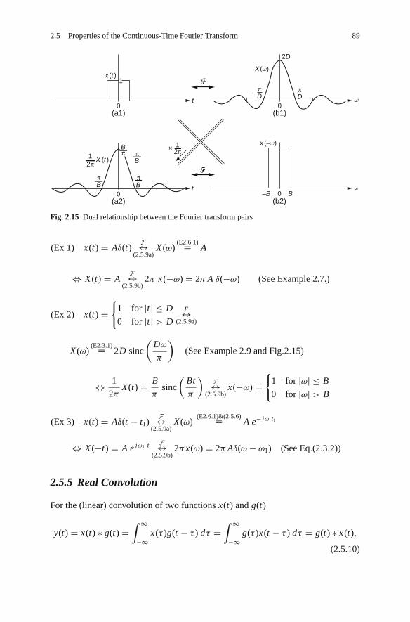
2.5 Properties of the Continuous-Time Fourier Transform 89
0
0
12π
0
0
π–
(b1)
(b2)(a2)
2D
B–B
(a1)
1x (t )
X (t )
X (ω )
x (–ω )
ω
ω
t
t
DπD
Bπ
1× 2π
πB
πB
– πB
Fig. 2.15 Dual relationship between the Fourier transform pairs
(Ex 1) x(t) = Aδ(t)F↔
(2.5.9a)X (ω)
(E2.6.1)= A
⇔ X (t) = AF↔
(2.5.9b)2π x(−ω) = 2π A δ(−ω) (See Example 2.7.)
(Ex 2) x(t) ={
1 for |t | ≤ D
0 for |t | > D
F↔(2.5.9a)
X (ω)(E2.3.1)= 2D sinc
(Dω
π
)(See Example 2.9 and Fig.2.15)
⇔ 1
2πX (t) = B
πsinc
(Bt
π
)F↔
(2.5.9b)x(−ω) =
{1 for |ω| ≤ B
0 for |ω| > B
(Ex 3) x(t) = Aδ(t − t1)F↔
(2.5.9a)X (ω)
(E2.6.1)&(2.5.6)= A e− jω t1
⇔ X (−t) = A e jω1 t F↔(2.5.9b)
2πx(ω) = 2π Aδ(ω − ω1) (See Eq.(2.3.2))
2.5.5 Real Convolution
For the (linear) convolution of two functions x(t) and g(t)
y(t) = x(t) ∗ g(t) =∫ ∞
−∞x(τ )g(t − τ ) dτ =
∫ ∞
−∞g(τ )x(t − τ ) dτ = g(t) ∗ x(t),
(2.5.10)

90 2 Continuous-Time Fourier Analysis
we can get its Fourier transform as
Y (ω) = F{y(t)} (2.2.1a)=(2.5.10)
∫ ∞
−∞
{ ∫ ∞
−∞x(τ )g(t − τ ) dτ
}e− jωt dt
=∫ ∞
−∞x(τ )e− jωτ
{ ∫ ∞
−∞g(t − τ )e− jω (t−τ ) dt
}dτ
t−τ→t=(2.2.1a)
∫ ∞
−∞x(τ )e− jωτ G(ω) dτ = G(ω)
∫ ∞
−∞x (τ )e− jωτ dτ
(2.2.1a)= G(ω)X (ω)
y(t) = x(t) ∗ g(t)F↔ Y (ω) = X (ω) G(ω) (2.5.11)
where Y (ω) = F{y(t)}, X (ω) = F{x(t)}, and G(ω) = F{g(t)}. This is thefrequency-domain input-output relationship of a linear time-invariant (LTI) systemwith the input x(t), the output y(t), and the impulse response g(t) where G(ω) iscalled the frequency response of the system.
On the other hand, if two functions xP (t) and gP (t) are periodic with com-mon period P , their linear convolution does not converge so that we need anotherdefinition of convolution, which is the periodic or circular convolution with theintegration performed over one period:
yP (t) = xP (t) ∗P
gP (t) =∫
PxP (τ )gP (t − τ ) dτ
=∫
PgP (τ )xP (t − τ ) dτ = gP (t) ∗
PxP (t) (2.5.12)
where ∗P
denotes the circular convolution with period P . Like the Fourier transform
of a linear convolution, the Fourier series coefficient of the periodic (circular) con-volution turns out to be the multiplication of the Fourier series coefficients of twoperiodic functions xP (t) and gP (t) (see Problem 2.8(a)):
yP (t) = xP (t) ∗P
gP (t)Fourier series↔ Yk = Xk Gk (2.5.13)
where Yk , Xk , and Gk are the Fourier coefficients of yP (t), xP (t), and gP (t),respectively.
2.5.6 Complex Convolution (Modulation/Windowing)
In duality with the convolution property (2.5.11) that convolution in the timedomain corresponds to multiplication in the frequency domain, we may expect the

2.5 Properties of the Continuous-Time Fourier Transform 91
modulation property that multiplication in the time domain corresponds to convolu-tion in the frequency domain:
y(t) = x(t)m(t)F↔ Y (ω) = 1
2πX (ω) ∗ M(ω) (2.5.14)
where Y (ω) = F{y(t)}, X (ω) = F{x(t)}, and M(ω) = F{m(t)}.On the other hand, if two functions xP (t) and m P (t) are periodic with common
period P , then their multiplication is also periodic and its Fourier series coefficientcan be obtained from the convolution sum (see Problem 2.8(b)):
yP (t) = xP (t)m P (t)Fourier series↔ Yk = 1
P
∑∞n=−∞ Xn Mk−n (2.5.15)
where Yk , Xk , and Mk are the Fourier coefficients of yP (t), xP (t), and m P (t),respectively.
Example 2.12 Sinusoidal Amplitude Modulation and Demodulation
(a) Sinusoidal Amplitude ModulationConsider a sinusoidal amplitude-modulated (AM) signal
xm(t) = x(t)m(t) = x(t) cos(ωct) (E2.12.1)
Noting that the Fourier transform of the carrier signal m(t) = cos(ωc t) is
M(ω) = F{m(t)} = F{cos(ωct)} (E2.11.2)= π (δ(ω + ωc) + δ(ω − ωc))(E2.12.2)
we can use the modulation property (2.5.14) to get the Fourier transform of theAM signal as
Xm(ω) = F{xm(t)} = F{x(t) cos ωc t} (2.5.14)= 1
2πX (ω) ∗ M(ω)
(E2.12.2)= 1
2πX (ω) ∗ π (δ(ω + ωc) + δ(ω − ωc))
(1.1.22)= 1
2(X (ω + ωc) + X (ω − ωc)) (E2.12.3)
This implies that the spectrum of the AM signal x(t) cos(ωct) consists of thesum of two shifted and scaled versions of X (ω) = F{x(t)}. Note that this resultcan also be obtained by applying the frequency shifting property (2.5.7) to thefollowing expression:
xm(t) = x(t) cos(ωct)(D.21)= 1
2(x(t)e jωct + x(t) e− jωct ) (E2.12.4)

92 2 Continuous-Time Fourier Analysis
(b) Sinusoidal Amplitude DemodulationIn an AM communication system, the receiver demodulates the modulatedsignal xm(t) by multiplying the carrier signal as is done at the transmitter:
xd (t) = 2xm(t) cos(ωct) (E2.12.5)
We can use the modulation property (2.5.14) together with Eqs. (E2.12.3)and (E2.12.2) to express the Fourier transform of the demodulated signal interms of the signal spectrum X (ω) as
Xd (ω) = F{xd (t)} = F{xm(t)2 cos ωc t} (2.5.14)= 1
2πXm(ω) ∗ 2 M(ω)
(E2.12.2)=(E2.12.3)
1
2π
1
2(X (ω + ωc) + X (ω − ωc)) ∗ 2π (δ(ω + ωc) + δ(ω − ωc))
(1.1.22)= 1
2(X (ω + 2ωc) + X (ω) + X (ω) + X (ω − 2ωc))
= 1
2X (ω + 2ωc) + X (ω) + 1
2X (ω − 2ωc) (E2.12.6)
Example 2.13 Ideal (Impulse or Instant) Sampler and Finite Pulsewidth Sampler
(a) Ideal SamplingWe can describe the output of the ideal (or impulse or instant) sampler to agiven input x(t) as
x∗(t) = x(t) δT (t)(δT (t) =
∑∞m=−∞ δ(t − mT ) : the impulse train
)(E2.13.1)
This is illustrated in Fig. 2.16(a1). Here, the switching function has been mod-eled as an impulse train with period T and its Fourier transform is given byEq. (E2.10.3) as
DT (ω)(E2.10.3)= 2π
T
∑∞k=−∞ δ(ω + kωs) with ωs = 2π
T(E2.13.2)
which is shown in Fig. 2.16(c1). We can use the modulation property (2.5.14)together with Eq. (E2.13.2) to express the Fourier transform of the ideal sampleroutput in terms of the input spectrum X (ω) as
X∗(ω)(2.5.14)= 1
2πX (ω) ∗ DT (ω)
(E2.13.2)= 1
T
∑∞k=−∞ X (ω) ∗ δ(ω + kωs)
(1.1.22)= 1
T
∑∞k=−∞ X (ω + kωs) (E2.13.3)
which is depicted in Fig. 2.16(d1).

2.5 Properties of the Continuous-Time Fourier Transform 93
(a1) Output of an ideal (impulse) sampler (a2) Output of a finite pulsewidth sampler
(b) The spectrum of a signal
(c1) The spectrum of the impulse train δT(t)
(d1) Output spectrum of the ideal sampler (d2) Output spectrum of the finite pulsewidth sampler
(c2) The spectrum of the rectangular wave rD/T(t)~
~
0 T 2T 3T 4T 5T 0 TD 2T 3T 4T 5Tt t
x (t) x (t)
x*(t) = x (t) δT (t) xs (t) = x (t) rD/T(t)
RD/T(ω)�T (ω)
X(ω)
–ωx ωxω
8π–T
6π–T
4π–T
02π–T
2πT
4πT
6πT
8πT
8π–T
6π–T
4π–T
02π–T
2πT
4πT
6πT
8πT
8π–T
6π–T
4π–T
02π–T
2πT
4πT
6πT
8πT
8π–T
6π–T
4π–T
02π–T
2πT
4πT
6πT
8πT
ω
ω ω
ω
X* (ω) X(ω)*�r(ω)12π= X* (ω) X(ω)*RD/T(ω)1
2π=
Fig. 2.16 Ideal sampler and finite pulsewidth sampler
(b) Finite Pulsewidth SamplingWe can describe the output of a finite pulsewidth sampler with period T to agiven input x(t) as
xs(t) = x(t) rD/T (t) (E2.13.4)
(rD/T (t) : a rectangular wave with duration D and period T )
This is illustrated in Fig. 2.16(a2). Here, the switching function has been mod-eled as a rectangular wave, rD/P (t), with duration D and period T . Noting thatfrom Eq. (E2.1.3), the Fourier series representation of this rectangular wave is
rD/P (t)(E2.1.3)=
A=1,P=T
1
T
∑∞k=−∞ D sinc
(k
D
T
)e jkωs t with ωs = 2π
T
(E2.13.5)

94 2 Continuous-Time Fourier Analysis
we can use Eq. (2.3.3) to write its Fourier transform as
RD/P (ω)(2.3.2)=P=T
2π
T
∑∞k=−∞ ck δ(ω − kωs) with ck = D sinc
(k
D
T
)
(E2.13.6)
which is shown in Fig. 2.16(c2). Now we can apply the modulation property(2.5.14) together with Eq. (E2.13.6) to express the Fourier transform of thefinite pulsewidth sampler output in terms of the input spectrum X (ω) as
Xs(ω)(2.5.14)= 1
2πX (ω) ∗ RD/P (ω)
(E2.13.6)= 1
T
∑∞k=−∞ X (ω) ∗ ck δ(ω − kωs)
(1.1.22)= 1
T
∑∞k=−∞ ck X (ω − kωs) (E2.13.7)
which is depicted in Fig. 2.16(d2).
2.5.7 Time Differential/Integration – FrequencyMultiplication/Division
By differentiating both sides of the inverse Fourier transform formula (2.2.1b) w.r.t.t , we obtain
dx(t)
dt
(2.2.1b)= 1
2π
∫ ∞
−∞X (ω)
(d
dte jωt
)dω = 1
2π
∫ ∞
−∞( jωX (ω))e jωt dω (2.5.16)
which yields the time-differentiation property of the Fourier transform as
dx(t)
dtF←→ jωX (ω) (2.5.17)
This means that differentiation in the time domain results in multiplication by jω inthe frequency domain.
On the other hand, the time-integration property is obtained by expressingthe integration of x(t) in the form of the convolution of x(t) and the unit stepfunction us(t) and then applying the convolution property (2.5.11) together withEq. (E2.8.6) as
∫ t
−∞x(τ ) dτ =
∫ ∞
−∞x(τ ) us(t − τ ) dτ = x(t) ∗ us(t)
F↔(2.5.11)
F{x(t)}F{us(t)} (E2.8.6)= π X (ω)δ(ω) + 1
jωX (ω) = π X (0)δ(ω) + 1
jωX (ω)
(2.5.18)

2.5 Properties of the Continuous-Time Fourier Transform 95
where the additional impulse term π X (0)δ(ω) on the RHS reflects the DC valueresulting from the integration. This equation is slightly above our intuition thatintegration/differentiation in the time domain results in division/multiplication byjω in the frequency domain.
The differentiation/integration properties (2.5.17)/(2.5.18) imply that differenti-ating/integrating a signal increases the high/low frequency components, respectivelybecause the magnitude spectrum is multiplied by | jω| = ω (proportional to fre-quency ω) or |1/jω| = 1/ω (inversely proportional to frequency ω). That is why adifferentiating filter on the image frame is used to highlight the edge at which thebrightness changes rapidly, while an integrating filter is used to remove impulse-likenoises. Note also that a differentiator type filter tends to amplify high-frequencynoise components and an integrator type filter would blur the image.
2.5.8 Frequency Differentiation – Time Multiplication
By differentiating both sides of the Fourier transform formula (2.2.1a) w.r.t. ω, weobtain
d X (ω)
dω
(2.2.1a)=∫ ∞
−∞x(t)
(d
dωe− jωt
)dt = − j
∫ ∞
−∞(t x(t))e− jωt dt (2.5.19)
which yields the frequency-differentiation property of the Fourier transform as
t x(t)F↔ j
d X (ω)
dω(2.5.20)
This means that multiplication by t in the time domain results in differentiation w.r.t.ω and multiplication by j in the frequency domain.
2.5.9 Time and Frequency Scaling
The Fourier transform of x(at) scaled along the time axis can be obtained as
F{x(at)} =∫ ∞
−∞x(at) e− jωt dt
t=τ/a= 1
|a|∫ ∞
−∞x(τ )e− jωτ/adτ
(2.2.1a)= 1
|a| X(ω
a
)
which yields the time and frequency scaling property of Fourier transform:
x(at)F↔ 1
|a| X(ω
a
)(2.5.21)
This is another example of the dual (inverse) relationship between time and fre-quency. A common illustration of this property is the effect on frequency contents of

96 2 Continuous-Time Fourier Analysis
playing back an audio tape at different speeds. If the playback speed is higher/slowerthan the recording speed, corresponding to compression(a>1)/expansion(a<1) intime, then the playback sounds get higher/lower, corresponding to expansion/compression in frequency.
2.5.10 Parseval’s Relation (Rayleigh Theorem)
If x(t) has finite energy and F{x(t)} = X (ω), then we have
∫ ∞
−∞|x(t)|2 dt = 1
2π
∫ ∞
−∞|X (ω)|2 dω (2.5.22)
(Proof) ∫ ∞
−∞|x(t)|2 dt =
∫ ∞
−∞x(t)x∗(t) dt
(2.2.1b)=∫ ∞
−∞x(t)
{1
2π
∫ ∞
−∞X∗(ω)e− jωt dω
}dt
= 1
2π
∫ ∞
−∞X∗(ω)
{∫ ∞
−∞x(t) e− jωt dt
}dω
(2.2.1a)= 1
2π
∫ ∞
−∞X∗(ω)X (ω) dω = 1
2π
∫ ∞
−∞|X (ω)|2 dω
This implies that the total energy in the signal x(t) can be determined either byintegrating |x(t)|2 over all time or by integrating |X (ω)|2/2π over all frequencies.For this reason, |X (ω)|2 is called the energy-density spectrum of the signal x(t).
On the other hand, if xP (t) is periodic with period P and its Fourier seriescoefficients are Xk’s, then we have an analogous relation∫ ∞
−∞|xP (t)|2 dt = 1
P
∑∞k=−∞ |Xk |2 (2.5.23)
where |Xk |2/P is called the power-density spectrum of the periodic signal xP (t).
2.6 Polar Representation and Graphical Plot of CTFT
Noting that a signal x(t) can be completely recovered from its Fourier trans-form X (ω) via the inverse Fourier transform formula (2.3.1b), we may say thatX (ω) contains all the information in x(t). In this section we consider the polaror magnitude-phase representation of X (ω) to gain more insight to the (generallycomplex-valued) Fourier transform. We can write it as
X (ω) = |X (ω)|∠X (ω)

2.6 Polar Representation and Graphical Plot of CTFT 97
(a) φ1 = φ2 = φ3 = 0 [rad]
t
t
t
(b) φ1 = 3 [rad], φ2 = 6 [rad], and φ3 = 9 [rad]
(c) φ1 = 3 [rad], φ2 = 2 [rad], and φ3 = 1 [rad]
0
0
0
Fig. 2.17 Plots of x(t) = 0.5 cos(2π t − φ1) + cos(4π t − φ2) + (2/3) cos(6π t − φ3) with differentphases
where |X (ω)| and ∠X (ω) give us the information about the magnitudes and phasesof the complex exponentials making up x(t). Notice that if x(t) is real, |X (ω)| is aneven function of ω and ∠X (ω) is an odd function of ω and thus we need to plot thespectrum for ω ≥ 0 only (see Sect. 2.5.2).
The signals having the same magnitude spectrum may look very different depend-ing on their phase spectra, which is illustrated in Fig. 2.17. Therefore, in someinstances phase distortion may be serious.
2.6.1 Linear Phase
There is a particular type of phase characteristic, called linear phase, that the phaseshift at frequency ω is a linear function of ω. Specifically, the Fourier transform ofx(t) changed in the phase by −αω, by the time shifting property (2.5.6), simplyresults in a time-shifted version x(t − α):
X1(ω) = X (ω)∠ − αω = X (ω)e− jαω F↔ x1(t) = x(t − α) (2.6.1)
For example, Fig. 2.17(b) illustrates how the linear phase shift affects the shapeof x(t).
2.6.2 Bode Plot
To show a Fourier transform X (ω), we often use a graphical representation consist-ing of the plots of the magnitude |X (ω)| and phase ∠X (ω) as functions of frequencyω. Although this is useful and will be used extensively in this book, we introduce
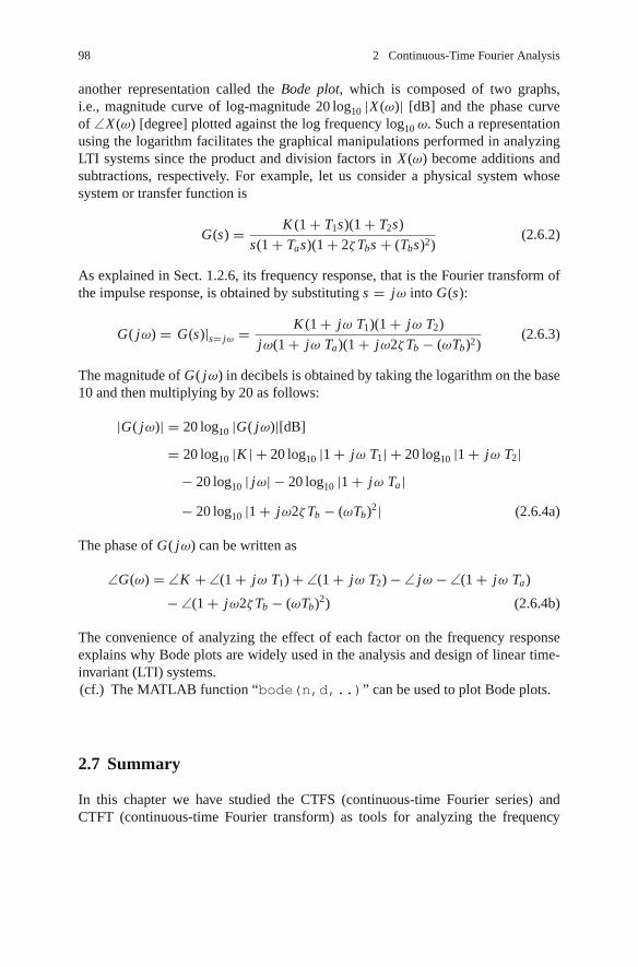
98 2 Continuous-Time Fourier Analysis
another representation called the Bode plot, which is composed of two graphs,i.e., magnitude curve of log-magnitude 20 log10 |X (ω)| [dB] and the phase curveof ∠X (ω) [degree] plotted against the log frequency log10 ω. Such a representationusing the logarithm facilitates the graphical manipulations performed in analyzingLTI systems since the product and division factors in X (ω) become additions andsubtractions, respectively. For example, let us consider a physical system whosesystem or transfer function is
G(s) = K (1 + T1s)(1 + T2s)
s(1 + Tas)(1 + 2ζ Tbs + (Tbs)2)(2.6.2)
As explained in Sect. 1.2.6, its frequency response, that is the Fourier transform ofthe impulse response, is obtained by substituting s = jω into G(s):
G( jω) = G(s)|s= jω = K (1 + jω T1)(1 + jω T2)
jω(1 + jω Ta)(1 + jω2ζ Tb − (ωTb)2)(2.6.3)
The magnitude of G( jω) in decibels is obtained by taking the logarithm on the base10 and then multiplying by 20 as follows:
|G( jω)| = 20 log10 |G( jω)|[dB]
= 20 log10 |K | + 20 log10 |1 + jω T1| + 20 log10 |1 + jω T2|− 20 log10 | jω| − 20 log10 |1 + jω Ta|− 20 log10 |1 + jω2ζ Tb − (ωTb)2| (2.6.4a)
The phase of G( jω) can be written as
∠G(ω) = ∠K + ∠(1 + jω T1) + ∠(1 + jω T2) − ∠ jω − ∠(1 + jω Ta)
− ∠(1 + jω2ζ Tb − (ωTb)2) (2.6.4b)
The convenience of analyzing the effect of each factor on the frequency responseexplains why Bode plots are widely used in the analysis and design of linear time-invariant (LTI) systems.(cf.) The MATLAB function “bode(n,d,..)” can be used to plot Bode plots.
2.7 Summary
In this chapter we have studied the CTFS (continuous-time Fourier series) andCTFT (continuous-time Fourier transform) as tools for analyzing the frequency

Problems 99
characteristic of continuous-time signals and systems. One of the primary motiva-tions for the use of Fourier analysis is the fact that we can use the Fourier series ortransform to represent most signals in terms of complex exponential signals whichare eigenfunctions of LTI systems (see Problem 2.14). The Fourier transform pos-sesses a wide variety of important properties. For example, the convolution propertyallows us to describe an LTI system in terms of its frequency response and the modu-lation property provides the basis for the frequency-domain analysis of modulation,sampling, and windowing techniques.
Problems
2.1 Fourier Series Analysis and Synthesis of Several Periodic Functions
(c) A half–rectified sinusoidal wave
–4 –3 –2
–1/2
xf (t )xh(t )
xa(t ) xb(t )
1/2 2
1
–2
–1–3
–6
3
6
1 2 3 4
(d) A full–rectified sinusoidal wave
(b) A triangular wave(a) A stair wave
–2
–4
–1
1
0 2 4 6 8
1
–1/2 2t
t
1/2t
t0
00
–8 –6 –2
Fig. P2.1
(a) Noting that the stair wave in Fig. P2.1(a) can be regarded as the sumof three scaled/time-shifted rectangular (square) waves with commonperiod 6[s] and different durations
xa(t) = 6r3/6(t − 1.5) − 3 + 3r1/6(t − 1.5) − 3r1/6(t − 4.5), (P2.1.1)
use Eq. (E2.1.3) together with (2.1.9) to find its complex exponentialFourier series coefficients. Then complete the following MATLAB pro-gram “cir02p 01a.m” and run it to plot the Fourier series representation(2.1.7) to see if it becomes close to xa(t) as the number of terms inthe summation increases, say, from 5 to 20. Also, compare the Fouriercoefficients with those obtained by using “CtFS exponential()”.

100 2 Continuous-Time Fourier Analysis
%cir02p 01a.mclear, clfP= 6; w0= 2*pi/P; % Period, Fundamental frequencytt=[-400:400]*P/400; % time interval of 4 periodsx = ’x a’; N=20; k= -N:N; % the range of frequency indicesc= 6*3*sinc(k*3/P).*exp(-j*1.5*k*w0)+3*sinc(k/P).*exp(-j*1.5*k*w0) ...
- ?????????????????????????????;c(N+1) = c(N+1) - ???;% [c n,k] = CtFS exponential(x,P,N);xt = feval(x,tt); % original signaljkw0t= j*k.’*w0*tt; xht = real((c/P)*exp(jkw0t)); % Eq. (2.1.5a)subplot(221), plot(tt,xt,’k-’, tt,xht,’r:’)c mag = abs(c); c phase = angle(c);subplot(222), stem(k, c mag)function y=x a(t)P=6; t= mod(t,P);y= 3*(0<=t&t<1) +6*(1<=t&t<2) +3*(2<=t&t<3) ...
-3*(3<=t&t<4) -6*(4<=t&t<5) -3*(5<=t&t<6);
(b) Use Eqs. (E.2.1.6) together with (2.1.9) to find the complex exponentialFourier series coefficients for the triangular wave in Fig. P2.1(b). Thencompose a MATLAB program, say, “cir02p01b.m” to plot the Fourierseries representation (2.1.7) and run it to see if the Fourier series repre-sentation becomes close to xb(t) as the number of terms in the summationincreases, say, from 3 to 6. Also, compare the Fourier coefficients withthose obtained by using “CtFS exponential()”.
(c) Consider a half-wave rectified cosine wave xh(t) = max(cos ω0t, 0),which is depicted in Fig. P2.1(c). We can use Eq. (2.1.5b) to obtain theFourier coefficients as
ck =∫ P/4
−P/4cos ω0te− jkω0t dt
= 1
2
∫ P/4
−P/4(e jω0t + e− jω0t )e− jkω0t dt with ω0 = 2π
P= π
k �=1or−1= 1
2
(1
− j(k − 1)ω0e− j(k−1)ω0t + 1
− j(k + 1)ω0e− j(k+1)ω0t
)∣∣∣∣1/2
−1/2
= 1
(k − 1)πsin(k − 1)
π
2+ 1
(k + 1)πsin(k + 1)
π
2
k=2m(even)= (−1)m 1
π
(1
k + 1− 1
k − 1
)= (−1)m+12
(k2 − 1)π(P2.1.2)
ckk=1or−1=
∫ P/4
−P/4(e jω0t + e− jω0t )e± jω0t dt
= 1
2
∫ P/4
−P/4(1 + e± j2ω0t )dt = P
4= 1
2(P2.1.3)
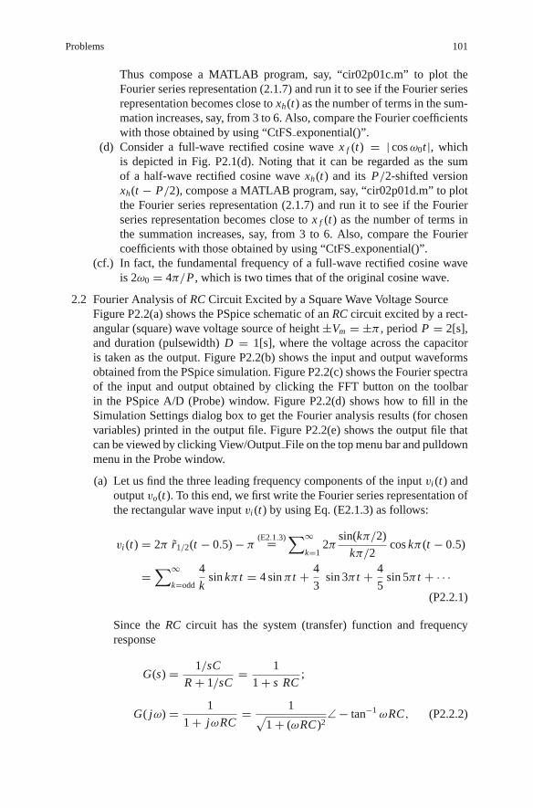
Problems 101
Thus compose a MATLAB program, say, “cir02p01c.m” to plot theFourier series representation (2.1.7) and run it to see if the Fourier seriesrepresentation becomes close to xh(t) as the number of terms in the sum-mation increases, say, from 3 to 6. Also, compare the Fourier coefficientswith those obtained by using “CtFS exponential()”.
(d) Consider a full-wave rectified cosine wave x f (t) = | cos ω0t |, whichis depicted in Fig. P2.1(d). Noting that it can be regarded as the sumof a half-wave rectified cosine wave xh(t) and its P/2-shifted versionxh(t − P/2), compose a MATLAB program, say, “cir02p01d.m” to plotthe Fourier series representation (2.1.7) and run it to see if the Fourierseries representation becomes close to x f (t) as the number of terms inthe summation increases, say, from 3 to 6. Also, compare the Fouriercoefficients with those obtained by using “CtFS exponential()”.
(cf.) In fact, the fundamental frequency of a full-wave rectified cosine waveis 2ω0 = 4π/P , which is two times that of the original cosine wave.
2.2 Fourier Analysis of RC Circuit Excited by a Square Wave Voltage SourceFigure P2.2(a) shows the PSpice schematic of an RC circuit excited by a rect-angular (square) wave voltage source of height ±Vm = ±π , period P = 2[s],and duration (pulsewidth) D = 1[s], where the voltage across the capacitoris taken as the output. Figure P2.2(b) shows the input and output waveformsobtained from the PSpice simulation. Figure P2.2(c) shows the Fourier spectraof the input and output obtained by clicking the FFT button on the toolbarin the PSpice A/D (Probe) window. Figure P2.2(d) shows how to fill in theSimulation Settings dialog box to get the Fourier analysis results (for chosenvariables) printed in the output file. Figure P2.2(e) shows the output file thatcan be viewed by clicking View/Output File on the top menu bar and pulldownmenu in the Probe window.
(a) Let us find the three leading frequency components of the input vi (t) andoutput vo(t). To this end, we first write the Fourier series representation ofthe rectangular wave input vi (t) by using Eq. (E2.1.3) as follows:
vi (t) = 2π r1/2(t − 0.5) − π(E2.1.3)=
∑∞k=1
2πsin(kπ/2)
kπ/2cos kπ (t − 0.5)
=∑∞
k=odd
4
ksin kπ t = 4 sin π t + 4
3sin 3π t + 4
5sin 5π t + · · ·
(P2.2.1)
Since the RC circuit has the system (transfer) function and frequencyresponse
G(s) = 1/sC
R + 1/sC= 1
1 + s RC;
G( jω) = 1
1 + jωRC= 1√
1 + (ωRC)2∠ − tan−1 ωRC, (P2.2.2)

102 2 Continuous-Time Fourier Analysis
(d) Simulation Settings window and Transient Output File Options dialog box
(a) PSpice schematic for the RC circuit excited by a square-wave source
V1= –3.14159V2= 3.14159TD = 0 (Delay Time)
VPULSE
TR = 0 (Rise Time)
PER = 2(PERiod)
TF = 0 (Falling Time)PW = 1 (Pulse Width/Duration)
0
V R 1k
0.3m
C
V
νi (t ) νo(t )+
−
+−
(b) The input and output voltage waveforms
4.0V
–4.0V0 sV(C : 2) V(VPULSE: +)
5 s Time 10 s
0V
νo
νi
(c) The FFT spectra of the input and output voltages
5.0V
2.5V
A1 = 500.000m, 4.00022.91111.3334
444.678m800.015m166.148m
A2 = 500.000m,A1 = 1.5000,A2 = 1.5000,A1 = 2.5000,A2 = 2.5000,
0V0 0.5 Hz 1.5 Hz 2.5 Hz 5 Hz Frequency 10 Hz
V(C : 2) V(VPULSE: +)
Probe Cursor
Fig. P2.2 (continued)

Problems 103
(e) The PSpice output file with FFT analysis
Fig. P2.2 PSpice simulation and analysis for Problem 2.2
its output to the input vi (t) (described by Eq. (P2.2.1)) can be written as
vo(t) =∑∞
k=2m+1
4
k√
1 + (kω0 RC)2sin (k ω0t − tan−1 kω0 RC)
with ω0 = 2πP = π (P2.2.3)
Show that the three leading frequency components of the output pha-sor are
V(1)o
k=1= G( jω0)V(1)i = 4√
1 + (ω0 RC)2∠ − tan−1 ω0 RC
RC=0.3= 4√1 + (0.3π)2
∠ − tan−1 0.3π = 2.91∠ − 43.3o (P2.2.4)
V(3)o
k=3= G( j3ω0)V(3)i = 4
3√
1 + (3ω0 RC)2∠ − tan−1 3ω0 RC
RC=0.3= 4
3√
1 + (0.9π)2∠ − tan−1 0.9π = 0.4446∠ − 70.5o (P2.2.5)

104 2 Continuous-Time Fourier Analysis
V(5)o
k=5= G( j5ω0)V(5)i = 4
5√
1 + (5ω0 RC)2∠ − tan−1 5ω0 RC
RC=0.3= 4
5√
1 + (1.5π)2∠ − tan−1 1.5π = 0.166∠ − 78o (P2.2.6)
where the phases are taken with that of sin ωt as a reference in the sine-and-phase form of Fourier series representation in order to match thisFourier analysis result with that seen in the PSpice simulation output file(Fig. P2.2(e)).
(cf.) Note that PSpice uses the sine-and-phase form of Fourier seriesrepresentation for spectrum analysis as below:
x(t) = d ′0 +
∑∞k=1
d ′k sin(kω0t + φ′
k) (P2.2.7a)
where the Fourier coefficients are
d ′0 = a0 = d0, d ′
k =√
a2k + b2
k = dk, φ′k = tan−1(ak/bk) = φk + π/2
(P2.2.7b)The magnitude ratios among the leading three frequency components ofthe input and output are
input : |V(1)i | : |V(3)
i | : |V(5)i | = 4 :
4
3:
5
3= 15 : 5 : 3
output : |V(1)o | : |V(3)
o | : |V(5)o | = 2.91 : 0.4446 : 0.166 = 15 : 2.3 : 0.86
This implies that the relative magnitudes of high frequency componentsto low ones become smaller after the input signal passes through the filter.This is a piece of evidence that the RC circuit with the capacitor voltagetaken as the output functions as a lowpass filter.
(b) Find the Fourier analysis results on V(k)i ’s and V(k)
o ’s for k = 0 : 5(and compare them with those obtained from PSpice simulation in (a)) bycompleting and running the following MATLAB program “sig02p 02.m”,which uses the MATLAB function “Fourier analysis()” declared as
function [yt,Y,X]= Fourier analysis(n,d,x,P,N)
This function takes the numerator (n) and denominator (d) of the transferfunction G(s), the (periodic) input function (x) defined for at least oneperiod [−P/2,+P/2], the period (P), and the order (N) of Fourier analysisas the input arguments and produces the output (yt) for one period and thesine-and-phase form of Fourier coefficients Y and X of the output andinput (for k = 0, . . . , N).
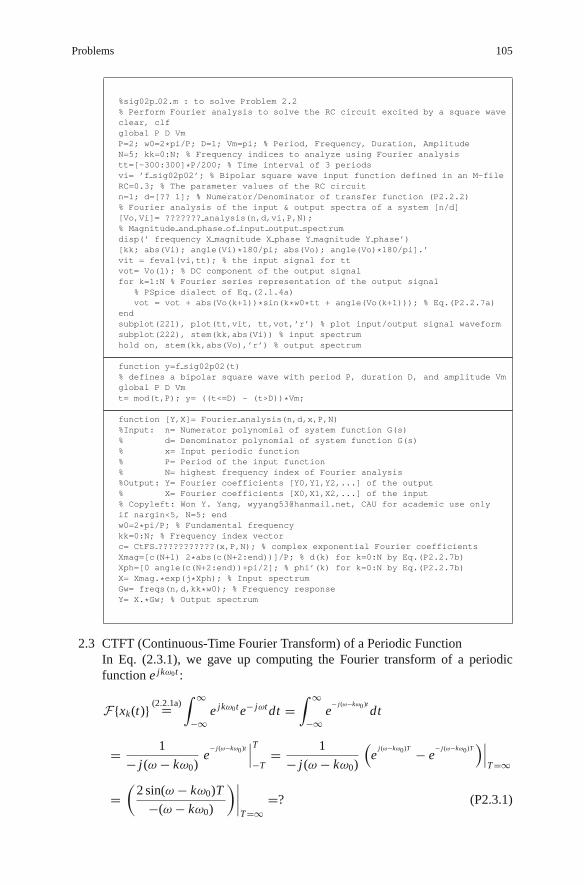
Problems 105
%sig02p 02.m : to solve Problem 2.2% Perform Fourier analysis to solve the RC circuit excited by a square waveclear, clfglobal P D VmP=2; w0=2*pi/P; D=1; Vm=pi; % Period, Frequency, Duration, AmplitudeN=5; kk=0:N; % Frequency indices to analyze using Fourier analysistt=[-300:300]*P/200; % Time interval of 3 periodsvi= ’f sig02p02’; % Bipolar square wave input function defined in an M-fileRC=0.3; % The parameter values of the RC circuitn=1; d=[?? 1]; % Numerator/Denominator of transfer function (P2.2.2)% Fourier analysis of the input & output spectra of a system [n/d][Vo,Vi]= ??????? analysis(n,d,vi,P,N);% Magnitude and phase of input output spectrumdisp(’ frequency X magnitude X phase Y magnitude Y phase’)[kk; abs(Vi); angle(Vi)*180/pi; abs(Vo); angle(Vo)*180/pi].’vit = feval(vi,tt); % the input signal for ttvot= Vo(1); % DC component of the output signalfor k=1:N % Fourier series representation of the output signal
% PSpice dialect of Eq.(2.1.4a)vot = vot + abs(Vo(k+1))*sin(k*w0*tt + angle(Vo(k+1))); % Eq.(P2.2.7a)
endsubplot(221), plot(tt,vit, tt,vot,’r’) % plot input/output signal waveformsubplot(222), stem(kk,abs(Vi)) % input spectrumhold on, stem(kk,abs(Vo),’r’) % output spectrum
function y=f sig02p02(t)% defines a bipolar square wave with period P, duration D, and amplitude Vmglobal P D Vmt= mod(t,P); y= ((t<=D) - (t>D))*Vm;
function [Y,X]= Fourier analysis(n,d,x,P,N)%Input: n= Numerator polynomial of system function G(s)% d= Denominator polynomial of system function G(s)% x= Input periodic function% P= Period of the input function% N= highest frequency index of Fourier analysis%Output: Y= Fourier coefficients [Y0,Y1,Y2,...] of the output% X= Fourier coefficients [X0,X1,X2,...] of the input% Copyleft: Won Y. Yang, [email protected], CAU for academic use onlyif nargin<5, N=5; endw0=2*pi/P; % Fundamental frequencykk=0:N; % Frequency index vectorc= CtFS ???????????(x,P,N); % complex exponential Fourier coefficientsXmag=[c(N+1) 2*abs(c(N+2:end))]/P; % d(k) for k=0:N by Eq.(P2.2.7b)Xph=[0 angle(c(N+2:end))+pi/2]; % phi’(k) for k=0:N by Eq.(P2.2.7b)X= Xmag.*exp(j*Xph); % Input spectrumGw= freqs(n,d,kk*w0); % Frequency responseY= X.*Gw; % Output spectrum
2.3 CTFT (Continuous-Time Fourier Transform) of a Periodic FunctionIn Eq. (2.3.1), we gave up computing the Fourier transform of a periodicfunction e jkω0t :
F{xk(t)} (2.2.1a)=∫ ∞
−∞e jkω0t e− jωt dt =
∫ ∞
−∞e
− j(ω−kω0)tdt
= 1
− j(ω − kω0)e
− j(ω−kω0)t∣∣∣T−T
= 1
− j(ω − kω0)
(e
j(ω−kω0)T − e− j(ω−kω0)T
)∣∣∣T =∞
=(
2 sin(ω − kω0)T
−(ω − kω0)
)∣∣∣∣T =∞
=? (P2.3.1)

106 2 Continuous-Time Fourier Analysis
Instead, we took a roundabout way of finding the inverse Fourier transformof 2πδ(ω − kω0) in expectation of that it will be the solution and showed thevalidity of the inverse relationship. Now, referring to Eq. (E2.6.2) or usingEq. (1.1.33a), retry to finish the derivation of Eq. (2.3.2) from Eq. (P2.3.1).
2.4 Two-Dimensional Fourier Transform of a Plane Impulse TrainThe two-dimensional (2-D) Fourier transform of a 2-D signal f (x, y) on thex-y plane such as an image frame is defined as
F(u, v) = F2 { f (x, y)} =∫ ∞
−∞
∫ ∞
−∞f (x, y)e− j(ux+vy)dx dy
=∫ ∞
−∞
(∫ ∞
−∞f (x, y)e− jux dx
)e− jvy dy (P2.4.1)
where x and y are the spatial cordinates and u and v are the spatial angularfrequencies [rad/m] representing how abruptly or smoothly f (x, y) changesw.r.t. the spatial shift along the x and y -axes, respectively.
(a) Show that the 2-D Fourier transform of f (x, y) = δ(y − αx) is
f (x, y) = δ(y − αx)F2↔ F(u, v) = 2π δ(u + αv) (P2.4.2)
(b) Show that the 2-D Fourier transform of f (x, y) = ∑∞n=−∞ δ(y − αx−
nd√
1 + α2) (Fig. P2.4(a)) is
F(u, v) =∫ ∞
−∞
∫ ∞
−∞
∑∞n=−∞ δ(y − αx − nd
√1 + α2)e− j(ux+vy)dx dy
(D.33)=∑∞
n=−∞
∫ ∞
−∞e− j(ux+v(αx+nd
√1+α2)) dx
=∑∞
n=−∞
∫ ∞
−∞e− j(u+αv)x dxe− jvnd
√1+α2
(2.3.2)=with ω=u+αv, t=x, k=0
∑∞n=−∞ 2πδ(u + αv)e− jvnd
√1+α2
(3.1.5)=with Ω=vd
√1+α2,Ω0=0
2πδ(u + αv)∑∞
i=−∞2πδ(vd√
1 + α2 − 2π i)
(1.1.34)= (2π )2
d√
1 + α2
∑∞i=−∞ δ(u + 2π iα
d√
1 + α2, v − 2π i
d√
1 + α2)
= (2π )2
d√
1 + α2
∑∞i=−∞ δ(u + 2π i
dsin θ, v − 2π i
dcos θ ) (P2.4.3)
as depicted in Fig. P2.4(b).2.5 ICTFT (Inverse Continuous-Time Fourier Transform) of Uo( jω) = 1/jω
Using Eq. (E2.3.3), show that the ICTFT of Uo( jω) = 1/jω is the oddcomponent of the unit step function:

Problems 107
(a) A 2–D (plane) impulse wave in the spatial domain (b) The 2–D Fourier transform depictedin the spatial frequency domain
Constant (DC)signal
Impulse train
Impulsespectrum
u
νu + αν = 0
θ1d
Impulse train
x
y
d
y – αx = 0
d sec θ = d
θθ
1 + tan2θ= d 1 + α2
Fig. P2.4 An example of 2-D Fourier transform
F−1{Uo( jω)} (2.2.1b)= 1
2π
∫ ∞
−∞
1
jωe jωt dω = 1
2sign(t) = uo(t) (P2.5.1)
which agrees with Eq. (E2.8.5).
2.6 Applications and Derivations of Several Fourier Transform Properties
(a) Applying the frequency shifting property (2.5.7) of Fourier transform toEq. (E2.7.1), derive Eq. (2.3.2).
(b) Applying the duality relation (2.5.9) to the time shifting property (2.5.6)of Fourier transform, derive the frequency shifting property (2.5.7).
(c) From the time-differentiation property (2.5.7) of Fourier tansform thatdifferentiation in the time domain corresponds to multiplication by jωin the frequency domain, one might conjecture that integration in thetime domain corresponds to division by jω in the frequency domain.But, Eq. (2.5.18) shows that the Fourier transform of
∫ t−∞ x(τ )dτ has an
additional impulse term reflecting the DC or average value of x(t). Canyou apply the time-differentiation property to Eq. (2.5.18) to derive theoriginal Fourier relation F{x(t)} = X (ω)?
∫ t
−∞x(τ )dτ
F↔ π X (0)δ(ω) + 1
jωX (ω) (2.5.18)
(d) Applying the duality relation (2.5.9) to the convolution property (2.5.11)of Fourier transform, derive the modulation property (2.5.14).
(e) Apply the time-differentiation property to the time-integration property(2.5.18) to derive the original Fourier relation F{x(τ )} = X (ω).
(f) Applying the time-differentiation property (2.5.7) to the time-domaininput-output relationship y(t) = dx(t)/dt of a differentiator, find thefrequency response of the differentiator.
(g) Applying the time-integration property (2.5.18) to the time-domain input-output relationship y(t) = ∫ t
−∞ x(τ )dτ of an integrator, find the frequency

108 2 Continuous-Time Fourier Analysis
response of the integrator on the assumption that the input has zeroDC value.
(h) Find the time-domain and frequency-domain input-output relationships ofa system whose impulse response is g(t) = δ(t − t0).
2.7 Fourier Transform of a Triangular PulseApplying the convolution property (2.5.11), find the Fourier transform of atriangular pulse DλD(t) (Eq. (1.2.25a)) obtained from the convolution of tworectangular pulses of height 1 and duration D.
2.8 Convolution/Modulation Properties of Fourier SeriesLet xP (t) and yP (t) be periodic functions with common period P that have thefollowing Fourier series representations, respectively:
xP (t) = 1
P
∑∞k=−∞ Xke jkω0t and yP (t) = 1
P
∑∞k=−∞ Yke jkω0t
(P2.8.1)
(a) The periodic or circular convolution of two periodic functions is defined as
z P (t) = xP (t) ∗ yP (t)(2.5.12)=
∫P
xP (τ )yP (t − τ )dτ
=∫
PyP (τ )xP (t − τ )dτ = yP (t) ∗ xP (t) (P2.8.2)
The product of the two Fourier series coefficients Xk and Yk is the Fourierseries coefficients of this convolution so that
z P (t) = 1
P
∑∞k=−∞ Zke jkω0t = 1
P
∑∞k=−∞ XkYke jkω0t (P2.8.3)
Applying the frequency shifting property (2.5.7) of Fourier transform toEq. (E2.7.1), derive Eq. (2.3.2).
(b) Show that the Fourier series coefficients of wP (t) = xP (t)yP (t) are
wP (t) = xP (t)yP (t)Fourier series↔
(2.5.15)Wk = 1
P
∑∞n=−∞ Xn Yk−n (P2.8.4)
so that we have
wP (t) = 1
P
∑∞k=−∞ Wke jkω0t (P2.8.5)
2.9 Overall Input-Output Relationship of Cascaded SystemConsider the systems of Fig. P2.9 consisting of two subsystems connected incascade, i.e., in such a way that the output of the previous stage is applied tothe input of the next stage. Note that the overall output y(t) can be expressedas the convolution of the input x(t) and the two subsystem’s impulse responses

Problems 109
g1(t) and g2(t) as
y(t) = g1(t) ∗ g2(t) ∗ x(t) = g2(t) ∗ g1(t) ∗ x(t). (P2.9.1)
Find the overall input-output relationship in the frequency domain.
(a) G1
G1G2
G1G2
G2x (t )
x (t )
y (t )
y (t )
y (t )
x (t )(b)
(c)
Fig. P2.9
2.10 Hilbert Transform and Analytic Signal
(a) Fourier Transform of Hilbert Transformed SignalThe Hilbert transform of a real-valued signal x(t) is defined as the convo-lution of x(t) and 1/π t or equivalently, the output of a Hilbert transformer(with the impulse response of h(t) = 1/π t) to the input x(t):
x(t) = h(t) ∗ x(t) = 1
π t∗ x(t) = 1
π
∫ ∞
−∞x(τ )
1
t − τdτ (P2.10.1)
- First, let us find the Fourier transform of h(t) = 1/π t by applying theduality (2.5.9) to Eq. (E2.8.5), which states that
1
2sign(t)
F↔ 1
jω
duality⇔ 1
j tF↔ ( ) (P2.10.2)
- We can multiply both sides by j/π to get the Fourier transform ofh(t) = 1/π t as
1
π tF↔ ( ) (P2.10.3)
- Now, we apply the convolution property to get the Fourier transform ofx(t) as
x(t) = 1
π t∗ x(t)
F↔convolution property
F(
1
π t
)F (x(t)) = ( ) X (ω) (P2.10.4)
This implies that the Hilbert transform has the effect of shifting thephase of positive/negative frequency components of x(t) by −90◦/+ 90◦,allowing the Hilbert transform a −90◦ phase shifter.

110 2 Continuous-Time Fourier Analysis
(b) Inverse Hilbert TransformNote that multiplying −H (ω) by the Fourier transform of the Hilberttransformed signal x(t) brings the spectrum back into that of the originalsignal x(t):
− H (ω)H (ω) X (ω) = −(− j sign(ω))(− j sign(ω)) X (ω ) = X (ω )(P2.10.5)
This implies the inverse Hilbert transform as
(−h(t)) ∗ x(t) =(
− 1
π t
)∗ 1
π t∗ x(t) = x(t) (P2.10.6)
(c) Analytic SignalThe analytic signal, or analytic representation, of a real-valued signal x(t)is defined as
xa(t) = x(t) + j x(t) (P2.10.7)
where x(t) is the Hilbert transform of x(t) and j is the imaginary unit.Show that the Fourier transform of the analytic signal is
Xa(ω) = F{x(t)} + jF{x(t)} ∼= 2us(ω)X (ω) (P2.10.8)
where us(ω) is the unit step function in frequency ω. This implies thatxa(t) has only nonnegative frequency component of x(t).
(d) Examples of Hilbert Transform and Analytic SignalShow that the following Hilbert transform relations hold:
cos(ωc t)H↔ sin(ωc t) (P2.10.9)
sin(ωct)H↔ −cos(ωct) (P2.10.10)
In general, it would be difficult to get the Hilbert transform of a signal x(t)directly from its definition (P2.10.1) and therefore, you had better take theinverse Fourier transform, X (ω), of x(t), multiply − j sign(ω), and thentake the inverse Fourier transform as
x(t) = F−1{− j sign(ω)X (ω)} (P2.10.11)
Now, let us consider a narrowband signal
s(t) = m(t) cos(ωct + φ) with m(t) : a baseband message signal(P2.10.12)
whose spectrum is (narrowly) bandlimited around the carrier frequencyωc. Show that the Hilbert transform of s(t) is

Problems 111
s(t) = m(t) cos(ωct + φ)H↔ s(t) = m(t) sin(ωct + φ) (P2.10.13)
Also, show that the analytic signal for s(t) can be expressed as
sa(t) = s(t) + j s(t) = m(t)e j(ωct+φ) (P2.10.14)
This implies that we can multiply the analytic signal by e− jωct to obtainthe envelope of the baseband message signal m(t).
(e) Programs for Hilbert TransformOne may wonder how the convolution in the time domain results in justthe phase shift. To satisfy your curiosity, try to understand the followingprogram “sig02p 10e.m”, which computes the output of a Hilbert trans-former to a cosine wave cos ωct with ωc = π/16 and sampling intervalTs = 1/16 [s]. For comparison, it uses the MATLAB built-in function“hilbert( )” to generate the analytic signal and take its imaginary partto get x(t).
(cf.) “hilbert( )” makes the Hilbert transform by using Eq. (P2.10.11).
%sig02p 10e.m% To try the Hilbert transform in the time/frequency domainclear, clfTs=1/16; t=[-149.5:149.5]*Ts; % Sample interval and Duration of h(t)h= 1/pi./t; % h(t): Impulse response of a Hilbert transformerNh=length(t); Nh2=floor(Nh/2); % Sample duration of noncausal parth = fliplr(h); % h(-t): Time-reversed version of h(t)wc= pi/16; % the frequency of an input signalNfft=512; Nfft2= Nfft/2; Nbuf=Nfft*2; % buffer sizett= zeros(1,Nbuf); x buf= zeros(1,Nbuf); xh buf= zeros(1,Nbuf);for n=-Nh:Nbuf-1 % To simulate the Hilbert transformer
tn=n*Ts; tt=[tt(2:end) tn];x buf = [x buf(2:end) cos(wc*tn)];xh buf = [xh buf(2:end) h *x buf(end-Nh+1:end).’*Ts];
endaxis limits= [tt([1 end]) -1.2 1.2];subplot(321), plot(tt,x buf), title(’x(t)’), axis(axis limits)subplot(323), plot(t(1:Nh2),h(1:Nh2), t(Nh2+1:end),h(Nh2+1:end))title(’h(t)’), axis([t([1 end]) -11 11])% To advance the delayed response of the causal Hilbert transformerxh = xh buf(Nh2+1:end); xh 1 = imag(hilbert(x buf));subplot(325), plot(tt(1:end-Nh2),xh,’k’, tt,xh 1), axis(axis limits)subplot(326), plot(tt,xh buf), axis(axis limits)ww= [-Nfft2:Nfft2]*(2*pi/Nfft);Xw= fftshift(fft(x buf,Nfft)); Xw= [Xw Xw(1)]; % X(w): spectrum of x(t)Xhw 1= fftshift(fft(xh 1,Nfft)); Xhw 1= [Xhw 1 Xhw 1(1)]; % Xh(w)norm(Xhw 1+j*sign(ww).*Xw)
In the program “sig02p 10e.m”, identify the statements performing thefollowing operations:
- The impulse response of the Hilbert transformer- Generating an input signal to the Hilbert transformer

112 2 Continuous-Time Fourier Analysis
- Computing the output expected to be the Hilbert transformed signal
Note the following:- The output sequence has been advanced by Nh/2 for comparison
with x(t) obtained using “hilbert ( )” because the real output ofthe causal Hilbert transformer is delayed by Nh/2, which is the lengthof the noncausal part of the Hilbert transformer impulseresponse h(n).
(f) Application of Hilbert Transform and Analytic Signal for EnvelopeDetectionTo see an application of Hilbert transform and analytic signal, considerthe following narrowband signal
s(t) = m(t) cos(ωct + φ)
= sinc
(B
πt
)cos(ωct + π
6) with B = 100, ωc = 400π (P2.10.15)
%sig02p 10f.m% To obtain the lowpass equivalent of Bandpass signalTs =0.001; fs =1/Ts; % Sampling Period/Frequencyt=[-511: 512]*Ts; % Duration of signalfc=200; wc=2*pi*fc; B=100; % Center frequency & bandwidth of signal s(t)m= sinc(B/pi*t);s= m.*cos(wc*t+pi/6); % a narrowband (bandpass) signalsa= hilbert(x); % Analytic signal sa(t) = s(t) + j sˆ(t)sl= sa.*exp(-j*wc*t); % Lowpass Equivalent (Complex envelope) sl(t)
Referring to the above program “sig02p 10f.m”, use the MATLAB func-tion “hilbert ( )” to make the analytic or pre-envelope signal sa(t),multiply it by e− jωct to get the lowpass equivalent or complex enve-lope sl(t), take its absolute values |sl(t)| to obtain the envelope of thebaseband message signal m(t), and plot it to compare with m(t) =|sinc (2Bt) |.
(g) Hilbert Transform with Real-Valued Signals for Signal DetectionConsider the system of Fig. P2.10 where a narrowband signal x(t) havingin-phase component xc(t) and quadrature component xs(t) is applied asan input to the system:
x(t) = xc(t) cos ωct − xs(t) sin ωct (P2.10.16)
Verify that the two outputs of the system are the same as xc(t) and xs(t),respectively by showing that their spectra are
Xc d (ω) = Xc(ω) and Xs d (ω) = Xs(ω) (P2.10.17)

Problems 113
Hilberttransformer
x (t )
x (t )
x (t )ˆx (t ) = xc (t ) cos ωct
–xs (t ) sin ωct
multiplier
multiplier
multiplier
summer
summer
sin ωct
–sin ωct
cos ωct
cos ωct
xc_d (t )
xs_d (t )
Fig. P2.10
Complete and run the following program “sig02p 10g.m” to check if theseresults are valid for
xc(t) = sinc (100t) , xs(t) = sinc (450t) , and ωc = 400π
Does the simulation result show that xc d (t) = xc(t) and xs d (t) = xs(t)?If one of them does not hold, figure out the reason of the discrepancy.
%sig02p 10g.m% To use the Hilbert transform for signal detectionclear, clfTs=0.0002; t=[-127:128]*Ts; % Sampling Period and Time intervalfc=200; wc=2*pi*fc; % Center frequency of signal x(t)B1=100*pi; B2=450*pi; % Bandwidth of signal x(t)xc= sinc(B1/pi*t); xs= sinc(B2/pi*t);x= xc.*cos(wc*t) - xs.*sin(wc*t);xh= imag(hilbert(x)); % imag(x(t)+j xˆ(t))=xˆ(t)xc d= x.*cos(wc*t) + xh.*?????????; % xc detectedxs d= -x.*sin(wc*t) + xh.*?????????; % xc detectedsubplot(221), plot(t,xc, t,xc d,’r’)subplot(222), plot(t,xs, t,xs d,’r’)norm(xc-xc d)/norm(xc), norm(xs-xs d)/norm(xs)
2.11 Spectrum Analysis of Amplitude Modulation (AM) Communication SystemConsider the AM communication system of Fig. P2.11(a) where the messagesignal x(t) is band-limited with maximum frequency ωx and the spectrumX (ω) is depicted in Fig. P2.11(b). Assume that the frequency response of the(bandpass) channel is
H (ω) ={
1 for |ω − ωc| < BC/2
0 elsewherewith BC ≥ 2ωx (P2.11.1)
and that of the LPF (lowpass filter) at the receiver side is

114 2 Continuous-Time Fourier Analysis
(e) The spectrum of the detected signal d (t )
(d) The spectrum of the demodulated signal xd(t )
(b) The spectrum of the message signal x(t )
(a) The block daigram of an AM communication system
messagesignal
multiplier multiplier
idealideal 2cos ωctcarrier signal cos ωct
ChannelH (ω)
LPFG (ω)
(c) The spectrum of the modulated, transmitted, and received signal r (t )
0
0
0
0
D (ω)
Xd (ω)
Xm (ω) = R (ω)
X (ω)
–2ωc 2ωc
–ωc
–ωx
ωc
ωx
ω
ω
ω
ω
x(t )r (t )xm(t ) xd(t )
d (t )
Fig. P2.11 An amplitude–modulation (AM) communication system
G(ω) ={
1 for |ω| < BR
0 elsewherewith ωx < BR < 2ωc − ωx (P2.11.2)
(a) Express the spectrum, Xd (ω), of the demodulated signal xd (t) in terms ofX (ω).
(b) Draw the spectra of the modulated and received signal r (t), the demod-ulated signal xd (t), and the detected signal d(t) on Fig. P2.11(c), (d),and (e).
(c) Complete and run the following program “sig02p 11.m” to simulate theAM communication system depicted in Fig. P2.11(a). Note that the spec-trum of each signal is computed by using the MATLAB built-in function“fft()” instead of CTFT (Continuous-Time Fourier Transform) sinceDFT (Discrete Fourier Transform) is applied to any sequence (consistingof sampled values of an arbitrary continuous-time signal), while CTFT

Problems 115
can be applied only to continuous-time signals expressed by a linearcombination of basic functions. DFT and “fft()” will be introducedin Chap. 4.
%sig02p 11.m% AM (amplitude-modulation) communication systemclear, clfTs=0.0001; t=[-127:128]*Ts; % Sampling Period and Time intervalfc=1000; wc=2*pi*fc; % Carrier frequencyB=1000; % (Signal) Bandwidth of x(t)x= sinc(B/pi*t).ˆ2; % a message signal x(t) having triangular spectrumxm= x.*cos(wc*t); % AM modulated signalr= xm; % received signalxd= r.*(2*?????????); % demodulated signalBr=wc/2; % (System) Bandwidth of an ideal LPFg= Br/pi*sinc(Br/pi*t); % (truncated) Impulse Response of the ideal LPFd= conv(xd,g)*Ts; % the output of the LPF to the demodulated signalsubplot(421), plot(t,x), title(’A message signal x(t)’)Nfft=256; Nfft2=Nff/2; % FFT size and a half of Nfftw= [-Nfft/2:Nfft/2]*(2*pi/Nfft/Ts); % Frequency vectorX= fftshift(fft(x)); X=[X X(1)]; % Spectrum of x(t)subplot(422), plot(w,abs(X)), title(’The spectrum X(w) of x(t)’)subplot(423), plot(t,xm), title(’The modulated signal xm(t)’)Xm= fftshift(fft(xm)); Xm=[Xm Xm(1)]; % Spectrum of modulated signalsubplot(424), plot(w,abs(Xm)), title(’The spectrum Xm(w) of xm(t)’)subplot(425), plot(t,xd), title(’The demodulated signal xd(t)’)Xd= fftshift(fft(xd)); Xd=[Xd Xd(1)]; % Spectrum of demodulated signalsubplot(426), plot(w,abs(Xd)), title(’The spectrum Xd(w) of xd(t)’)d= d(Nfft2+[0:Nfft-1]);subplot(427), plot(t,d), title(’The LPF output signal d(t)’)D= fftshift(fft(d)); D=[D D(1)]; % Spectrum of the LPF outputsubplot(428), plot(w,abs(D)), title(’The spectrum D(w) of d(t)’)
2.12 Amplitude-Shift Keying (ASK) and Frequency-Shift Keying (FSK)
(a) Amplitude-Shift Keying (ASK) or On-Off Keying (OOK)Find the spectrum X ASK (ω) of a BASK (binary amplitude-shift keying)or OOK modulated signal xASK (t) = rD(t) cos(ω1t) (Fig. P2.12(a)) whererD(t) is a unit-height rectangular pulse with duration D.
(b) Frequency-Shift Keying (FSK)Find the spectrum X F SK (ω) of a BFSK (binary frequency-shift keying)modulated signal xF SK (t) = rD(t) cos(ω1t) + rD(t − D) cos(ω2(t − D))(Fig. P2.12(b)).

116 2 Continuous-Time Fourier Analysis
0 0
(a) A BASK or OOK signal (b) A BFSK signal
rD(t ) cos(ω1t ) rD(t ) cos(ω1t ) rD (t – D ) cos(ω2(t – D ))
1 1
D D Dt t
Fig. P2.12
2.13 Autocorrelation/Crosscorrelation TheoremSuppose we have X (ω) = F{x(t)}, Y (ω) = F{y(t)}, and G(ω) = F{g(t)},where x(t), y(t), and g(t) are the real-valued input, output, and impulseresponse of an LTI system G so that
y(t) = g(t) ∗ x(t)F↔ Y (ω) = G(ω) ∗ X (ω) (P2.13.1)
(a) Prove the autocorrelation theorem:
Φxx (ω) = F{φxx (t)} (1.4.12a)= F{x(t) ∗ x(−t)} = |X (ω)|2
(Energy Density Spectrum) (P2.13.2)
(b) Prove the crosscorrelation theorem:
Φxy(ω) = F{φxy(t)} (1.4.12a)= F{x(t) ∗ y(−t)}
= X (ω)Y ∗(ω) = G∗(ω) |X (ω)|2 (P2.13.3)
(c) Prove that
Φyy(ω) = F{φyy(t)} (1.4.12a)= F{y(t) ∗ y∗(−t)} = Y (ω)Y ∗(ω)
= |G(ω)|2|X (ω)|2 (P2.13.4)
2.14 Power Theorem - Generalization of Parseval’s RelationProve the power theorem that, with X (ω) = F{x(t)} and Y (ω) = F{y(t)},we have ∫ ∞
−∞x(t)y∗(t)dt = 1
2π
∫ ∞
−∞X (ω)Y ∗(ω) dω (P2.14.1)
2.15 EigenfunctionIf the output of a system to an input is just a (possibly complex-valued) con-stant times the input, then the input signal is called an eigenfunction of thesystem. Show that the output of an LTI (linear time-invariant) system with the(causal) impulse response g(t) and system (transfer) function G(s) = L{g(t)}to a complex exponential input es0t is,

Problems 117
G{es0t } = g(t) ∗ es0t = G(s0)es0t with G(s0) = G(s)|s=s0(P2.15.1)
where G(s) is assumed not to have any pole at s = s0 so that the ampli-tude factor G(s0), called the eigenvalue, is finite. This implies that a complexexponential function is an eigenfunction of LTI systems.
2.16 Fourier Transform of a Polygonal Signal (Problem 4.20 of [O-1])
(a) Show that the Fourier trnasform of y(t) = (at + b)(us(t − t1) − us(t − t2))with t1 < t2 is
Y (ω) = 1
ω2(a+ jbω)(e− jωt2 −e− jωt1 )+ j
a
ω(t1e− jωt2 −t2e− jωt1 ) (P2.16.1)
(b) We can describe a triangular pulse having three vertices (ti−1, 0), (ti , xi ),and (ti+1, 0) as
λ i (t) ={
xi + xiti −ti−1
(t − ti ) = − xi ti−1
ti −ti−1+ xi
ti −ti−1t for ti−1 ≤ t < ti
xi + xiti −ti+1
(t − ti ) = − xi ti+1
ti −ti+1+ xi
ti −ti+1t for ti ≤ t < ti+1
(P2.16.2)
(a) A signal and its polygonal approximation (b) A trapezoidal signal
x (t )
z (t )
x3x4
xP (t )
xn –1 xn
x2x1
t0 t1 t2 t3 t4 . . . tn –1 –T2 –T1 T1 T2
T2 – T1
0tn
x0 t t
Fig. P2.16
Use Eq. (P2.16.1) to show that the Fourier transform of this pulse is
Λi (ω) = 1
ω2
{xi
ti − ti−1(e− jωti − e− jωti−1 ) + xi
ti+1 − ti(e− jωti − e− jωti+1 )
}
(P2.16.3)
(c) Fig. P2.16(a) shows a finite-duration signal x(t) and its piece-wise linearor polygonal approximation xP (t) where x(t) = xP (t) = 0 ∀t ≤ t0 andt ≥ tn . Use Eq. (P2.16.3) to show that the Fourier transform of xP (t) is
X P (ω) = F{xP (t)} = F{∑n
i=0λi (t)
}= 1
ω2
∑n
i=0ki e
− jωti (P2.16.4)

118 2 Continuous-Time Fourier Analysis
where
ki = (ti−1 − ti )xi+1 + (ti − ti+1)xi−1 + (ti+1 − ti−1)xi
(ti − ti−1)(ti+1 − ti )and
x(t−1) = x(tn+1) = 0
Complete the following program “CTFT poly ()” so that it implementsthis method of computing the Fourier transform.
function [X,w]=CTFT poly(t,x,w)% Computes the CTFT of x(t) for frequency w by using Eq.(P2.16.4).N =length(x); n=1:N;if nargin<3, w = [-100:100]*pi/100+1e-6; endt=[2*t(1)-t(2) t 2*t(N)-t(N-1)]; x=[0 x 0];X= 0;for i=2:N+1
ki=((t(i-1)-t(i))*x(i+1)+(t(i)-t(i+1))*x(i-1)+(t(i+1)-t(i-1))*x(i));k(i)= ki/(t(i)-t(i-1))/(t(i+1)-t(i));X= X + k(i)*exp(-j*w*t(i));
endX = X./(w.ˆ2+eps);
(d) For the trapezoidal signal z(t) shown in Figure P2.16(b), find its Fouriertransform Z (ω) in two ways:
(i) Regarding z(t) as the convolution of two unit-height rectangularpulses each of length D1 = T2 − T1 and D2 = T2 + T1, you canuse the convolution property (2.5.11) together with Eq. (E2.3.2).
(ii) Use Eq. (P2.16.4), which is the result of part (c).(iii) Use the MATLAB routine “CTFT poly ()” to get Z (ω) = F{z(t)}
with T1 = 1 and T2 = 2 and plot it to compare the result with thatobtained (i) or (ii).<Hint> You can complete and run the following program.
%sig02p 16.m% Numerical approximation of CTFT for a trapezoidal signalclear, clfT1=1; T2=2; D1= T2-T1; D2= T1+T2;t= [-T2 -T1 T1 T2];x= [0 T2-T1 T2-T1 0];w= [-200:200]/100*pi+1e-6; % frequency range on which to plot X(w)X= D1*D2*sinc(w*D1/2/pi).*sinc(w*D2/2/pi);X poly= ?????????(?,?,?); % (P2.16.4)Discrepancy=norm(X poly-X)plot(w,abs(X),’b’, w,abs(X poly),’r’)
(e) Show that, if we choose the points ti ’s sufficiently close together so thatthe piecewise linear approximation, xP (t), of x(t) is accurate enough tosatisfy the bounded error condition

Problems 119
|x(t) − xP (t)| ≤ ε, (P2.16.5)
then the Fourier transform (Eq. (P2.16.4)) of xP (t) is close to X (ω) =F{x(t)} enough to satisfy
∫ ∞
−∞|X (ω) − X P (ω)|2dω ≤ 2π (tn − t0)ε2 (P2.16.6)
(cf.) This implies that even though a signal x(t) cannot be expressed as alinear combination, a multiplication, or convolution of basic functions,we can find its approximate Fourier transform from the collection ofsample values of x(t) and that we can improve the accuracy by makingthe piecewise approximation xP (t) closer to x(t).
(cf.) This result suggests us that it is possible to evaluate numerically theFourier transform for a finite-duration signal whose values are mea-sured experimentally at many (discrete) time instants, even though theclosed-form analytic expression of the signal is not available or toocomplicated to deal with.
2.17 Impulse Response and Frequency Response of Ideal Bandpass FilterConsider a sinc function multiplied by a cosine function, which is depicted inFig. P2.17:
Bt0
Fig. P2.17
g(t) = B
πsinc
(B
πt
)cos ωpt with ωp = 10B (P2.17.1)
(a) Using Eqs. (E2.9.1&2) and the amplitude modulation (AM) property(E2.12.3), find the Fourier transform G(ω) = F{g(t)} and sketch it.
(b) If Eq. (P2.17.1) describes the impulse response of a system, which typeof filter is it?(Lowpass, Bandpass, Highpass, Bandstop)
2.18 Design of Superheterodyne Receiver – Combination of Tunable/SelectiveFiltersWe can build a tunable selective filter, called the superheterodyne or super-sonic heterodyne receiver often abbreviated superhet), by combining a tun-able, but poorly selective filter, a highly-selective, but untunable filter having
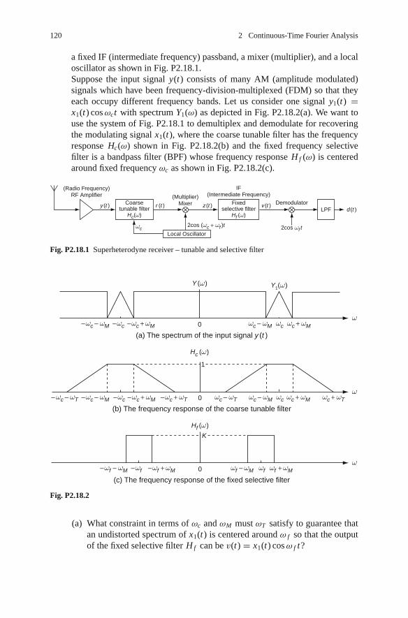
120 2 Continuous-Time Fourier Analysis
a fixed IF (intermediate frequency) passband, a mixer (multiplier), and a localoscillator as shown in Fig. P2.18.1.Suppose the input signal y(t) consists of many AM (amplitude modulated)signals which have been frequency-division-multiplexed (FDM) so that theyeach occupy different frequency bands. Let us consider one signal y1(t) =x1(t) cos ωct with spectrum Y1(ω) as depicted in Fig. P2.18.2(a). We want touse the system of Fig. P2.18.1 to demultiplex and demodulate for recoveringthe modulating signal x1(t), where the coarse tunable filter has the frequencyresponse Hc(ω) shown in Fig. P2.18.2(b) and the fixed frequency selectivefilter is a bandpass filter (BPF) whose frequency response H f (ω) is centeredaround fixed frequency ωc as shown in Fig. P2.18.2(c).
(Radio Frequency)RF Amplifier
Coarsetunable filter
Hc(ω)
(Multiplier)Mixer
Local Oscillator
Fixedselective filter
Hf (ω)
DemodulatorLPF
IF(Intermediate Frequency)
2cos (ωc + ωf )t 2cos ωf tωc
y (t ) r (t ) z (t ) v (t )d (t )
Fig. P2.18.1 Superheterodyne receiver – tunable and selective filter
(c) The frequency response of the fixed selective filter
0ω
Hf (ω )
K
– ωf – ωM – ωf + ωM– ωf ωf – ωM ωf
+ ωMωf
(b) The frequency response of the coarse tunable filter
0
1
– ωc + ωM – ωc + ωT ωc + ωM ωc + ωTωωc– ωc – ωT ωc – ωT ωc – ωM– ωc – ωM – ωc
Hc (ω )
(a) The spectrum of the input signal y (t )
0– ωc + ωM ωc – ωM
Y (ω ) Y1(ω )
ωc + ωMω
ωc– ωc – ωM – ωc
Fig. P2.18.2
(a) What constraint in terms of ωc and ωM must ωT satisfy to guarantee thatan undistorted spectrum of x1(t) is centered around ω f so that the outputof the fixed selective filter H f can be v(t) = x1(t) cos ω f t?

Problems 121
(b) Determine and sketch the spectra R(ω), Z (ω), V (ω), and D(ω) of theoutput r (t) of the coarse tunable filter Hc, the input z(t) and output v(t) ofthe fixed selective filter H f , and the output d(t) of the LPF.
(c) How could you determine the gain K of the fixed selective filter H f
required to have v(t) = x1(t) cos ω f t at its output?(d) Complete and run the following program “sig02p 18.m” to simulate the
superheterodyne receiver twice, once with kT = 18 and once with kT =19. Explain why the two simulation results are so different in terms of theerror between d(t) and x1(t). Note that the parameters kc, kf, kM, and kTcorrespond to ωc, ω f , ωM , and ωT , respectively.
%sig02p 18.m
% simulates a superheterodyne receiver combining a coarse tunable filter
% and a fixed selective filter
% Copyleft: Won Y. Yang, [email protected], CAU for academic use only
clear, clf
N=128; kc=16; kf=12; kM=4; kT=12; Wcf=2*pi/N*(kc+kf); Wf=2*pi/N*kf;
%create a signal having the spectrum as Fig.P2.17.2(a)
n=[0:N-1]; kk=[-N/2:N/2]; % Time/Frequency ranges
y=make signal(N,kc,kM);
Y=fftshift(fft(y)); Y mag= abs([Y Y(1)]);
subplot(6,2,1), plot(n,y), title(’y(t)’)
subplot(6,2,2), plot(kk,Y mag), title(’Y(w)’)
%tunable filter
r=??????????????(N,kc,kM,kT,?);
R=fftshift(fft(r)); R mag= abs([R R(1)]);
subplot(6,2,3), plot(n,r), title(’r(t) after tunable filter’)
subplot(6,2,4), plot(kk,R mag), title(’R(w)’)
%modulation
z=r.*(????????????);
Z=fftshift(fft(z)); Z mag= abs([Z Z(1)]);
subplot(6,2,5), plot(n,z), title(’z(t) after modulation’)
subplot(6,2,6), plot(kk,Z mag), title(’Z(w)’)
%selective filter
K=1; v=????????????????(N,kf,kM,K,?);
V=fftshift(fft(v)); V mag= abs([V V(1)]);
subplot(6,2,7), plot(n,v), title(’v(t) after selective filter’)
subplot(6,2,8), plot(kk,V mag), title(’V(w)’)
%demodulation
d0=v.*(???????????);
D0=fftshift(fft(d0)); D0 mag= abs([D0 D0(1)]);
subplot(6,2,9), plot(n,d0), title(’d0(t) after demodulation’)
subplot(6,2,10), plot(kk,D0 mag), title(’D0(w)’)
%tunable filter as LPF
d=tunable filter(N,0,kM,kT,d0);
D=fftshift(fft(d)); D mag= abs([D D(1)]);
x1=zeros(1,N);
for k=-kM:kM, x1(n+1)= x1(n+1)+(1-abs(k)/kM)*cos(2*pi*k*n/N); end
subplot(6,2,11), plot(n,d,’b’, n,x1,’r’)
title(’detected/transmitted signal’)
subplot(6,2,12), plot(kk,D mag),
title(’Spectrum D(w) of detected signal’)
error between detected transmitted signals= norm(d-x1)

122 2 Continuous-Time Fourier Analysis
function x=make signal(N,kc,kM)
% create a signal having the spectrum as Fig.P2.17.2(a)
n=1:N;
x=zeros(1,N);
for k=0:N/2-1
tmp= 2*pi*k*(n-1)/N;
if k<kc-kM, x(n)= x(n)+sin(tmp);
elseif k>kc+kM, x(n)=x(n)+sin(tmp); % whatever, cos() or sin()
else x(n)= x(n)+(1-abs(k-kc)/kM)*cos(tmp);
end
end
function x t=tunable filter(N,kc,kM,kT,x)
% BPF with passband (kc-kM,kc+kM) and
% stopband edge frequencies kc-kT and kc+kT
X=fft(x,N);
for k=1:N/2+1
if k<=kc-kT|k>kc+kT+1, X(k)=0; X(N+2-k)=0;
elseif k<=kc-kM+1
X(k)=X(k)*(1-(kc-kM-k+1)/(kT-kM)); X(N+2-k)=conj(X(k));
elseif k>kc+kM
X(k)=X(k)*(1-(k-1-kc-kM)/(kT-kM)); X(N+2-k)=conj(X(k));
end
end
x t=real(ifft(X,N));
function x t=selective filter(N,kf,kM,K,x)
% passes only the freq (kf-kM,kf+kM) with the gain K
X=fft(x,N);
for k=1:N
if (k>kf-kM&k<=kf+kM+1)|(k>N-kf-kM&k<=N-kf+kM+1), X(k)= K*X(k);
else X(k)=0;
end
end
x t=real(ifft(X));
2.19 The Poisson Sum Formula (PSF) and Spectrum of Sampled SignalConsider an LTI (linear time-invariant) system with impulse response h(t)and frequency response H ( jω) = F{h(t)}. Note that the response (output)of the system to the impulse train can be expressed in terms of the impulseresponse as
δ(t)G{}→ h(t); δT (t) =
∑∞n=−∞ δ(t − nT )
G{}→∑∞
n=−∞ h(t − nT ) (P2.19.1)
Likewise, the response (output) of the system to a single or multiple complexexponential signal can be written as
e jkω0t G{}→ H ( jkω0)e jkω0t ;1
T
∑∞k=−∞ e jkω0t G{}→ 1
T
∑∞k=−∞ H ( jkω0)e jkω0t
(P2.19.2)
(a) Based on the above results (P2.19.1) & (P2.19.2) and Eq. (2.1.10), provethat, for any function h(t) with its Fourier transform H ( jω) = F{h(t)}well-defined, the following relation holds:
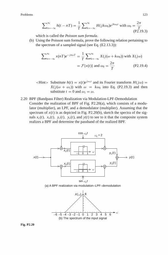
Problems 123
∑∞n=−∞ h(t − nT ) = 1
T
∑∞k=−∞ H ( jkω0)e jkω0t with ω0 = 2π
T(P2.19.3)
which is called the Poisson sum formula.(b) Using the Poisson sum formula, prove the following relation pertaining to
the spectrum of a sampled signal (see Eq. (E2.13.3)):
∑∞n=−∞ x(nT )e− jnωT = 1
T
∑∞k=−∞ X ( j(ω + kω0)) with X ( jω)
= F{x(t)} and ω0 = 2π
T(P2.19.4)
<Hint> Substitute h(t) = x(t)e jω1t and its Fourier transform H ( jω) =X ( j(ω + ω1)) with ω = kω0 into Eq. (P2.19.3) and thensubstitute t = 0 and ω1 = ω.
2.20 BPF (Bandpass Filter) Realization via Modulation-LPF-DemodulationConsider the realization of BPF of Fig. P2.20(a), which consists of a modu-lator (multiplier), an LPF, and a demodulator (multiplier). Assuming that thespectrum of x(t) is as depicted in Fig. P2.20(b), sketch the spectra of the sig-nals xc(t), xs(t), yc(t), ys(t), and y(t) to see to it that the composite systemrealizes a BPF and determine the passband of the realized BPF.
(a) A BPF realization via modulation–LPF–demodulation
(b) The spectrum of the input signal
x(t)
xc(t )yc(t )
y(t )
ys(t )xs(t )
2
–1 0 1
X(ω)
cos ωct
sin ωct
ω
2
–1 0 1ω
ω–6 –5 –4 –3 –2 –1 0 1 2
8
3 4 5 6
ωc = 2
Fig. P2.20

124 2 Continuous-Time Fourier Analysis
2.21 TDM (Time-Division Multiplexing)As depicted in Fig. P2.21(a), Time-Division multiplexing (TDM) is to transmittwo or more PAM (pulse amplitude modulation) signals not simultaneously assubchannels (separated in the frequency-domain), but physically by turns inone communication channel where each subchannel is assigned a timeslot ofduration D every T s in such a way that the timeslots do not overlap. Sketch aTDM waveform of two signals x1(t) and x2(t) in Fig. P2.21(b).
x1(t ) x1(t )p1(t )
x2(t )p2(t )x2(t )
Communicationchannel
synchronizedswitching
(a) A TDM communication system
x1(t )
x2(t )
t
t
t(b) A time–division multiplexed signal
Fig. P2.21 TDM (Time-Division Multiplexing) communication
2.22 FDM (Frequency-Division Multiplexing)As depicted in Fig. P2.22(a), Frequency-Division multiplexing (FDM) is totransmit two or more SAM (sinusoidal amplitude modulation) signals as sub-carriers (separated in the frequency-domain) in such a way that the frequencyslots each carrying a signal (amplitude-modulated with different carrier fre-quency) do not overlap. Assuming that the channel is ideal so that r (t) = s(t),sketch the spectrum of the FDM signal to be transmitted over the same com-munication channel where the spectra of two signals x1(t) and x2(t) to befrequency-multiplexed are shown in Fig. P2.22(b).
(cf.) Time/frequency-division multiplexing assigns different time/frequencyintervals to each signal or subchannel.
2.23 Quadrature MultiplexingConsider the quadrature multiplexing system depicted in Fig. P2.22, wherethe two signals are assumed to be bandlimited, that is,
X1(ω) = X2(ω) = 0 for ω > ωM (P2.23.1)
as illustrated in Fig. P2.23(b).
(a) Assuming that the channel is ideal so that r (t) = s(t), express the spectraS(ω), V1(ω), V2(ω), Y1(ω), Y2(ω) of the signals s(t), v1(t), v2(t), y1(t),and y2(t) in terms of X1(ω) and X2(ω).
(b) Complete and run the following MATLAB program “sig02p 23.m” to seeif y1(t) = x1(t) and y2(t) = x2(t).

Problems 125
(a) A FDM (Frequency–Division Multiplexing) communication system
x1(t )
s (t )
cos ω1t
cos ω2t
–ω 1 –ω M ω M
–ω M ω M
0
1 2
21
ω 1
–ω 2 0 ω 2
Communicationchannel
r (t )
y1(t )
y2(t )x2(t )
(b) The spectra of two signals to be frequency–division multiplexed
–ωM ωM0
X1(ω) X2(ω)
ω–ωM ωM0
ω
Fig. P2.22 FDM (Frequency-Division Multiplexing) communication
x1(t )
s (t ) r (t )
cos ωct
sin ωct
–ωM ωM
–ωM ωM
Communicationchannel
x2(t )
v1(t ) y1(t )
y2(t )
2
2v2(t )
Fig. P2.23 Quadrature multiplexing
%sig02p 23.m% Quadrature Multiplexing in Fig.P2.23% Copyleft: Won Y. Yang, [email protected], CAU for academic use onlyclear, clfN=128; kc=16; kM=6; kx1=6; kx2=6; Wc=2*pi/N*kc;n=[0:N-1]; kk=[-N/2:N/2];x1= make signal1(N,kx1); x2= make signal2(N,kx2);X1= fftshift(fft(x1)); X2= fftshift(fft(x2));subplot(523), plot(kk,abs([X1 X1(1)])), title(’X1(w)’)subplot(524), plot(kk,abs([X2 X2(1)])), title(’X2(w)’)s= x1.*???(Wc*n) + x2.*sin(Wc*n); S= fftshift(fft(s));subplot(513), plot(kk,abs([S S(1)])), title(’S(w)’)v1= s.*cos(Wc*n); V1= fftshift(fft(v1));v2= s.*???(Wc*n); V2= fftshift(fft(v2));subplot(527), plot(kk,abs([V1 V1(1)])), title(’V1(w)’)subplot(528), plot(kk,abs([V2 V2(1)])), title(’V2(w)’)

126 2 Continuous-Time Fourier Analysis
% selective filter(ideal LPF)kf=0; K=2;y1= selective filter(N,kf,kM,K,v1); Y1= fftshift(fft(y1));y2= ????????????????(N,kf,kM,K,v2); Y2= fftshift(fft(y2));discrepancy1=norm(x1-y1), discrepancy2=norm(x2-y2)subplot(529), plot(kk,abs([Y1 Y1(1)])), title(’Y1(w)’)subplot(5,2,10), plot(kk,abs([Y2 Y2(1)])), title(’Y2(w)’)
function x=make signal1(N,kx)n=1:N; kk=1:kx-1; x= (1-kk/kx)*cos(2*pi*kk.’*n/N);
function x=make signal2(N,kx)n=1:N; kk=1:kx-1; x= kk/kx*cos(2*pi*kk.’*n/N);
2.24 Least Squares Error (LSE) and Fourier Series RepresentationConsider a continuous-time function x(t) on a time interval [a, b] and a set ofits sampled values, {x1, x2, · · · , xN } (with xn = x(tn)). Let us find an approx-imate representation of x(t) as a linear combination of some basis functions{φk(t); k = 1 : K }:
x(c, t) =∑K
k=1ck φk(t) for a ≤ t ≤ b (P2.24.1)
where the coefficient vector c = [c1 c2 · · · cK ]T is to be determined so that thefollowing objective function can be minimized:
E2(c) =∫ b
a(x(t) − x(c, t))2dt (P2.24.2)
E2(c) =∑K
n=1(xn − x(c, tn))2 (P2.24.3)
The following notations will be used:
x = [x1 x2 · · · xN ]T with xn = x(tn) (P2.24.4a)
c = [c1 c2 · · · cK ]T (P2.24.4b)
ϕ(t) = [φ1(t) φ2(t) · · · φK (t)]T (P2.24.4c)
ε = [ε1 ε2 · · · εN ]T (P2.24.4d)

Problems 127
with εn = xn − x(c, tn) = xn −∑K
k=1ckφk(tn) = xn − ϕT (tn)c
Φ =
⎡⎢⎢⎢⎢⎣
ϕT (t1)ϕT (t2)
••
ϕT (tN )
⎤⎥⎥⎥⎥⎦ =
⎡⎢⎢⎢⎢⎣
φ11 φ21 • φK 1
φ12 φ22 • φK 2
• • • •• • • •
φ1N φ2N • φK N
⎤⎥⎥⎥⎥⎦ with φkn = φk(tn) (P2.24.4e)
Based on these notations, the above objective function (P2.24.3) can bewritten as
E2(c) = ε∗T ε = [x∗ − Φ∗c∗]T [x − Φc]
= x∗T x − x∗T Φc − c∗T Φ∗T x + c∗T Φ∗T Φc
= x∗T[I − Φ[Φ∗T Φ]−1Φ∗T
]x
+ [ΦT Φ∗c∗ − ΦT x∗]T [Φ∗T Φ]−1[Φ∗T Φc − Φ∗T x] (P2.24.5)
where only the second term of this equation depends on c. Note that thisobjective function is minimized for
Φ∗T Φc − Φ∗T x = 0 (a normal equation); c = [Φ∗T Φ]−1Φ∗T x (P2.24.6)
(a) Let the K functions {φk(t), k = 1 : K } constitute an orthogonal set forthe N discrete times {tn, n = 1 : N } in the sense that
∑N
n=1φ∗
knφmn = 0 ∀ k �= m (P2.24.7)
so that [Φ∗T Φ] is diagonal. Show that the coefficients can be deter-mined as
ck =∑N
n=1 xnφ∗kn∑N
n=1 φ∗knφkn
, for k = 1, 2, · · · , K (P2.24.8)
Likewise, if the K functions {φk(t), k = 1 : K } constitute an orthogonalset for the continuous time intrerval [a, b] in the sense that
∫ b
aφ∗
k (t)φm(t) dt = 0 ∀ k �= m, (P2.24.9)
then the coefficients can be determined as
ck =∫ b
a x(t)φ∗k (t) dt∫ b
a φ∗k (t)φk(t) dt
, for k = 1, 2, · · · , K (P2.24.10)

128 2 Continuous-Time Fourier Analysis
(b) Using Eq. (P2.24.1), find an approximate representation of a real-valuedfunction x(t) for −P/2 ≤ t ≤ P/2 in terms of the following basisfunctions
φk(t) = 1
Pe jkω0t with ω0 = 2π
Pand k = −K : K (P2.24.11)

Chapter 3Discrete-Time Fourier Analysis
Contents
3.1 Discrete-Time Fourier Transform (DTFT) . . . . . . . . . . . . . . . . . . . . . . . . . . . . . . . . . . . . . . 1303.1.1 Definition and Convergence Conditions of DTFT Representation . . . . . . . . . . . 1303.1.2 Examples of DTFT Analysis . . . . . . . . . . . . . . . . . . . . . . . . . . . . . . . . . . . . . . . . . . 1323.1.3 DTFT of Periodic Sequences . . . . . . . . . . . . . . . . . . . . . . . . . . . . . . . . . . . . . . . . . 136
3.2 Properties of the Discrete-Time Fourier Transform . . . . . . . . . . . . . . . . . . . . . . . . . . . . . . 1383.2.1 Periodicity . . . . . . . . . . . . . . . . . . . . . . . . . . . . . . . . . . . . . . . . . . . . . . . . . . . . . . . . . 1383.2.2 Linearity . . . . . . . . . . . . . . . . . . . . . . . . . . . . . . . . . . . . . . . . . . . . . . . . . . . . . . . . . . 1383.2.3 (Conjugate) Symmetry . . . . . . . . . . . . . . . . . . . . . . . . . . . . . . . . . . . . . . . . . . . . . . . 1383.2.4 Time/Frequency Shifting (Real/Complex Translation) . . . . . . . . . . . . . . . . . . . . 1393.2.5 Real Convolution . . . . . . . . . . . . . . . . . . . . . . . . . . . . . . . . . . . . . . . . . . . . . . . . . . . 1393.2.6 Complex Convolution (Modulation/Windowing) . . . . . . . . . . . . . . . . . . . . . . . . . 1393.2.7 Differencing and Summation in Time . . . . . . . . . . . . . . . . . . . . . . . . . . . . . . . . . . 1433.2.8 Frequency Differentiation . . . . . . . . . . . . . . . . . . . . . . . . . . . . . . . . . . . . . . . . . . . . 1433.2.9 Time and Frequency Scaling . . . . . . . . . . . . . . . . . . . . . . . . . . . . . . . . . . . . . . . . . . 1433.2.10 Parseval’s Relation (Rayleigh Theorem) . . . . . . . . . . . . . . . . . . . . . . . . . . . . . . . . 144
3.3 Polar Representation and Graphical Plot of DTFT . . . . . . . . . . . . . . . . . . . . . . . . . . . . . . . 1443.4 Discrete Fourier Transform (DFT) . . . . . . . . . . . . . . . . . . . . . . . . . . . . . . . . . . . . . . . . . . . . 147
3.4.1 Properties of the DFT . . . . . . . . . . . . . . . . . . . . . . . . . . . . . . . . . . . . . . . . . . . . . . . 1493.4.2 Linear Convolution with DFT . . . . . . . . . . . . . . . . . . . . . . . . . . . . . . . . . . . . . . . . . 1523.4.3 DFT for Noncausal or Infinite-Duration Sequence . . . . . . . . . . . . . . . . . . . . . . . . 155
3.5 Relationship Among CTFS, CTFT, DTFT, and DFT . . . . . . . . . . . . . . . . . . . . . . . . . . . . . 1603.5.1 Relationship Between CTFS and DFT/DFS . . . . . . . . . . . . . . . . . . . . . . . . . . . . . 1603.5.2 Relationship Between CTFT and DTFT . . . . . . . . . . . . . . . . . . . . . . . . . . . . . . . . 1613.5.3 Relationship Among CTFS, CTFT, DTFT, and DFT/DFS . . . . . . . . . . . . . . . . . 162
3.6 Fast Fourier Transform (FFT) . . . . . . . . . . . . . . . . . . . . . . . . . . . . . . . . . . . . . . . . . . . . . . . . 1643.6.1 Decimation-in-Time (DIT) FFT . . . . . . . . . . . . . . . . . . . . . . . . . . . . . . . . . . . . . . . 1653.6.2 Decimation-in-Frequency (DIF) FFT . . . . . . . . . . . . . . . . . . . . . . . . . . . . . . . . . . . 1683.6.3 Computation of IDFT Using FFT Algorithm . . . . . . . . . . . . . . . . . . . . . . . . . . . . 169
3.7 Interpretation of DFT Results . . . . . . . . . . . . . . . . . . . . . . . . . . . . . . . . . . . . . . . . . . . . . . . . 1703.8 Effects of Signal Operations on DFT Spectrum . . . . . . . . . . . . . . . . . . . . . . . . . . . . . . . . . 1783.9 Short-Time Fourier Transform – Spectrogram . . . . . . . . . . . . . . . . . . . . . . . . . . . . . . . . . . 1803.10 Summary . . . . . . . . . . . . . . . . . . . . . . . . . . . . . . . . . . . . . . . . . . . . . . . . . . . . . . . . . . . . . . . . . 182
Problems . . . . . . . . . . . . . . . . . . . . . . . . . . . . . . . . . . . . . . . . . . . . . . . . . . . . . . . . . . . . . . . . . 182
In this chapter we study the discrete-time Fourier analysis techniques, i.e., theDTFT (Discrete-Time Fourier Transform), DFT (Discrete Fourier Transform), andDFS (Discrete Fourier Series) of a discrete-time sequence, which will be used to
W.Y. Yang et al., Signals and Systems with MATLAB R©,DOI 10.1007/978-3-540-92954-3 3, C© Springer-Verlag Berlin Heidelberg 2009
129

130 3 Discrete-Time Fourier Analysis
describe and analyze the frequency characteristics of discrete-time signals and thefrequency-domain behavior of discrete-time systems. We also deal with the fastFourier transform (FFT), which is a very efficient algorithm for computing the DFT.
Each of the continuous-time and discrete-time Fourier techniques has its ownapplication in the sense that they are used for analyzing continuous-time anddiscrete-time signals/systems, respectively. However, if you do not understand theirorganic inter-relationship beyond some similarity, you will miss the overall pointof viewing the frequency characteristic of signals/systems and get only a confusingimpression that there are too many Fourier techniques. Basically, we want to find,say, the CTFT of continuous-time signals since no inherently discrete-time signalsexists in the physical world. However, the DFT, implemented by the FFT algorithm,of discrete-time signals obtained by sampling continuous-time signals is the onlyone practical Fourier analysis technique because of its outstanding computationalconvenience compared with the CTFT that is difficult to compute for general sig-nals. That is why we need to know the relationship between the CTFT and DFT andultimately, be able to get the “true” information about the frequency characteristicof a (continuous-time) signal from its FFT-based spectrum.
3.1 Discrete-Time Fourier Transform (DTFT)
3.1.1 Definition and Convergence Conditions of DTFTRepresentation
As the discrete-time counterpart of the CTFT (continuous-time Fourier transform)
X ( jω) = F{x(t)} (2.2.1a)=∫ ∞
−∞x(t) e− jωt dt
we define the Fourier transform of a discrete-time sequence x[n] as
X ( jΩ) = X [e j Ω] = F{x [n]} =∑∞
n=−∞ x[n] e− j Ωn (3.1.1)
which is called the DTFT (discrete-time Fourier transform). From now on, we willmore often use X (Ω) than X ( jΩ) or X [e jΩ] for simplicity. Let us see the physicalmeaning of the DTFT.
Remark 3.1 Physical Meaning of the DTFT – Signal Spectrum and FrequencyResponse
(1) If a sequence x[n] represents a physical signal, its DTFT X (Ω) = F{x[n]}means the signal spectrum, which describes the frequency contents of the signal.
(2) In particular, if a time function g[n] represents the impulse response of adiscrete-time LTI (linear time-invariant) system, its DTFT G(Ω) = F{g[n]}means the frequency response, which describes how the system responds to a

3.1 Discrete-Time Fourier Transform (DTFT) 131
sinusoidal input sequence of digital (angular) frequency Ω (refer to Sect. 1.2.6for the definition of frequency response).
One striking difference of the DTFT from the CTFT is its periodicity (with period2π ) in the (digital) frequency variable Ω, which results from the fact that it is afunction of e jΩ periodic with period 2π in Ω, i.e., e j(Ω+2πn) = e jΩ. Based on theperiodicity of the DTFT, we are going to use the CTFS (for periodic functions) toderive the IDTFT (inverse discrete-time Fourier transform) formula. To this end, wecan use Eq. (2.1.5a) with P = 2π, ω0 = 2π/P = 1, t = Ω, and k = −n to writethe (continuous-frequency) Fourier series representation of X (Ω) as
X (Ω)(2.1.5a)= 1
2π
∑∞n=−∞ xn e− j Ωn (3.1.2a)
where the Fourier coefficients are
xn(2.1.5b)=
P=2π, ω0=1,t=Ω,k=−n
∫2π
X (Ω) e j Ωn dΩ (the integral over one period of length 2π )
(3.1.2b)
Noting that Eq. (3.1.2a) is the same as Eq. (3.1.1) multiplied by a scaling factor1/2π , we can multiply Eq. (3.1.2b) by the same scaling factor 1/2π to write theIDTFT formula as
x[n] = F−1{X (Ω)} = 1
2π
∫2π
X (Ω) e jΩn dΩ (3.1.3)
We call Eqs. (3.1.1) and (3.1.3) the DTFT pair where Eq. (3.1.1) is the analysisequation and Eq. (3.1.3) is the synthesis equation.
Like the convergence conditions (2.2.2a) and (2.2.2b) for the CTFT, it can bestated that the DTFT will exist if the sequence x[n] has finite energy, i.e.,
∑∞n=−∞ |x[n] |2 < ∞ (3.1.4a)
or if it is absolutely summable, i.e.,
∑∞n=−∞ |x[n] | < ∞ (3.1.4b)
Remark 3.2 Frequency Response Existence Condition and Stability Condition of aSystem
Note that, for the impulse response g[n] of a discrete-time LTI system, theabsolute-summability condition (3.1.4b) is identical with the stability condition(1.2.27b). This implies that a stable LTI system has a well-defined frequencyresponse G(Ω) = F{g[n]}.

132 3 Discrete-Time Fourier Analysis
3.1.2 Examples of DTFT Analysis
Example 3.1 DTFT of a Rectangular Pulse SequenceFor the rectangular pulse of duration 2M+1 from −M to M shown in Fig. 3.1(a1)
and described by
r ′2M+1[n] = us[n + M] − us[n − M − 1] (E3.1.1)
we can apply Eq. (3.1.1) to get its DTFT as
R′2M+1(Ω)
(3.1.1)=∑∞
n=−∞ r ′2M+1[n] e− j Ωn
(E3.1.1)=∑M
n=−Me− j Ωn (D.23)= e j ΩM 1 − e− j Ω(2M+1)
1 − e− j Ω(Dirichlet kernel)
= e j ΩM e− j Ω(2M+1)/2(e j Ω(2M+1)/2 − e− j Ω(2M+1)/2)
e− j Ω/2(e j Ω/2 − e− j Ω/2)(D.22)= sin(Ω(2M + 1)/2)
sin(Ω/2)(E3.1.2)
whose magnitude and phase are depicted in Fig. 3.1 (b1) and (c1), respectively.Likewise, for the rectangular pulse of duration 2M + 1 from 0 to 2M shown inFig. 3.1(a2) and described by
r2M+1[n] = us[n] − us[n − 2M − 1] = r ′2M+1 [n − M] (E3.1.3)
with M = 1
–1
–2π 2π–π π
1
1
0
(c1) (c2)
3
even-symmetric
odd-symmetric
0
–2π –2π 2π–π
–π
π
π
2π–π
–π
π
π
0 000
r2M +1[n]'
(a1) r2M +1[n]'
R2M +1(Ω)
Ω
Ω Ω
'
∠R2M +1(Ω)'
∠R2M +1(Ω)'
∠R2M +1(Ω)
∠R2M +1(Ω)
nwith M = 1
1 2
1
0
= r2M +1[n–M ]' r2M +1[n ]
n
(b1) R2M +1(Ω)'–2π 2π–π π0
R2M +1(Ω)
Ω
(b2) R2M +1(Ω)
3
(a2) r2M +1[n ] = r2M +1[n–M ]'
Fig. 3.1 Two rectangular pulse sequences and their magnitude & phase spectra
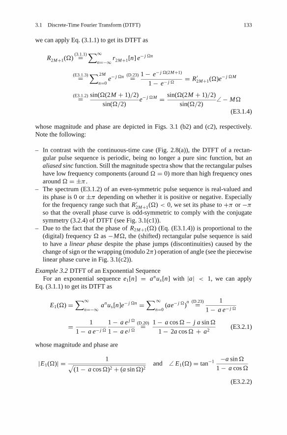
3.1 Discrete-Time Fourier Transform (DTFT) 133
we can apply Eq. (3.1.1) to get its DTFT as
R2M+1(Ω)(3.1.1)=
∑∞n=−∞ r2M+1[n] e− j Ωn
(E3.1.3)=∑ 2M
n=0e− j Ωn (D.23)= 1 − e− j Ω(2M+1)
1 − e− j Ω= R′
2M+1(Ω)e− j ΩM
(E3.1.2)= sin(Ω(2M + 1)/2)
sin(Ω/2)e− j ΩM = sin(Ω(2M + 1)/2)
sin(Ω/2)∠ − MΩ
(E3.1.4)
whose magnitude and phase are depicted in Figs. 3.1 (b2) and (c2), respectively.Note the following:
– In contrast with the continuous-time case (Fig. 2.8(a)), the DTFT of a rectan-gular pulse sequence is periodic, being no longer a pure sinc function, but analiased sinc function. Still the magnitude spectra show that the rectangular pulseshave low frequency components (around Ω = 0) more than high frequency onesaround Ω = ±π .
– The spectrum (E3.1.2) of an even-symmetric pulse sequence is real-valued andits phase is 0 or ±π depending on whether it is positive or negative. Especiallyfor the frequency range such that R′
2M+1(Ω) < 0, we set its phase to +π or −π
so that the overall phase curve is odd-symmetric to comply with the conjugatesymmetry (3.2.4) of DTFT (see Fig. 3.1(c1)).
– Due to the fact that the phase of R2M+1(Ω) (Eq. (E3.1.4)) is proportional to the(digital) frequency Ω as −MΩ, the (shifted) rectangular pulse sequence is saidto have a linear phase despite the phase jumps (discontinuities) caused by thechange of sign or the wrapping (modulo 2π ) operation of angle (see the piecewiselinear phase curve in Fig. 3.1(c2)).
Example 3.2 DTFT of an Exponential SequenceFor an exponential sequence e1[n] = anus[n] with |a| < 1, we can apply
Eq. (3.1.1) to get its DTFT as
E1(Ω) =∑∞
n=−∞ anus[n]e− j Ωn =∑∞
n=0(ae− j Ω)
n (D.23)= 1
1 − a e− j Ω
= 1
1 − a e− j Ω
1 − a e j Ω
1 − a e j Ω
(D.20)= 1 − a cos Ω − j a sin Ω
1 − 2a cos Ω + a2(E3.2.1)
whose magnitude and phase are
|E1(Ω)| = 1√(1 − a cos Ω)2 + (a sin Ω)2
and ∠ E1(Ω) = tan−1 −a sin Ω
1 − a cos Ω
(E3.2.2)

134 3 Discrete-Time Fourier Analysis
: a = 0.5: a = 0.8
: a = –0.5: a = –0.8
a = 0.8
a = 0.5
(a1) (a2)
nn
(b1) (b2)
(c1) (c2)
–2π 0
1
1
2π–π
π –2π 0 2π–π πa = –0.5
a = –0.8∠E1(Ω)
∠E1(Ω)
ΩΩ0
E1(Ω)a = 0.8
a = 0.5
–2π 0 2π–π π Ω
2
Ω
E1(Ω)
a = –0.8
2
4
–2π 0 2π–π π
a = –0.50
0
–1
1
Fig. 3.2 Four exponential sequences and their magnitude & phase spectra
Fig. 3.2(a1–a2), (b1–b2), and (c2–c2) show the exponential sequences e1[n] =anus[n] with a = ±0.5 and ±0.8 and their magnitude and phase spectra. Notethe following:
- From Fig. 3.2(a1), we see that e1[n] with a = 0.8 is smoother than that witha = 0.5. This is reflected in Fig. 3.2(b1) showing that the magnitude spectrum|E1[Ω]| with a = 0.8 is larger/smaller than that with a = 0.5 around Ω = 0 (lowfrequency)/ Ω = ±π (high frequency). Also from Fig. 3.2(a2), we see that e1[n]with a = −0.8 changes more rapidly than that with a = −0.5. This is reflectedin Fig. 3.2(b2) showing that the magnitude spectrum |E1[Ω]| with a = −0.8 islarger/smaller than that with a = −0.5 around Ω = ±π (high frequency)/Ω = 0(low frequency).
- Comparing Fig. 3.2(a1) and (a2), we see that e1[n] with a < 0 changes muchmore rapidly than that with a > 0. This is reflected in that the magnitudespectrum |E1[Ω]| with a < 0 (Fig. 3.2(b2)) is large around Ω = ±π (highfrequency) and that with a > 0 (Fig. 3.2(b1)) is large around Ω = 0 (lowfrequency).
Example 3.3 DTFT of a Symmetric Exponential SequenceFor the exponential sequence e2[n] = a|n| with |a| < 1, we can apply Eq. (3.1.1)
to get its DTFT as
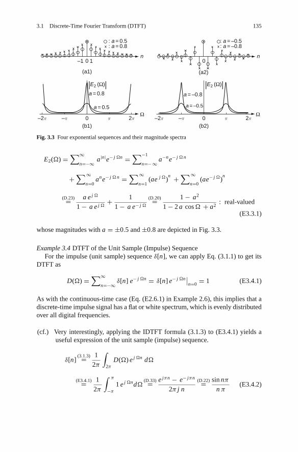
3.1 Discrete-Time Fourier Transform (DTFT) 135
–1 0
–2π 2π–π π0 –2π 2π–π π0
0nn
: a = 0.5: a = 0.8
a = 0.8 a = –0.8
a = 0.5 a = –0.5
(a1)
(b1) (b2)
(a2)
|E2 (Ω)|
Ω Ω
|E2 (Ω)|
: a = –0.5: a = –0.8
1
Fig. 3.3 Four exponential sequences and their magnitude spectra
E2(Ω) =∑∞
n=−∞ a|n|e− j Ωn =∑−1
n=− ∞ a−ne− j Ω n
+∑∞
n=0ane− j Ω n =
∑∞n=1
(ae j Ω)n +
∑∞n=0
(ae− j Ω)n
(D.23)= a e j Ω
1 − a e j Ω+ 1
1 − a e− j Ω
(D.20)= 1 − a2
1 − 2 a cos Ω + a2: real-valued
(E3.3.1)
whose magnitudes with a = ±0.5 and ±0.8 are depicted in Fig. 3.3.
Example 3.4 DTFT of the Unit Sample (Impulse) SequenceFor the impulse (unit sample) sequence δ[n], we can apply Eq. (3.1.1) to get its
DTFT as
D(Ω) =∑∞
n=−∞ δ[n] e− j Ωn = δ[n] e− j Ωn∣∣n=0 = 1 (E3.4.1)
As with the continuous-time case (Eq. (E2.6.1) in Example 2.6), this implies that adiscrete-time impulse signal has a flat or white spectrum, which is evenly distributedover all digital frequencies.
(cf.) Very interestingly, applying the IDTFT formula (3.1.3) to (E3.4.1) yields auseful expression of the unit sample (impulse) sequence.
δ[n](3.1.3)= 1
2π
∫2π
D(Ω) e j Ωn dΩ
(E3.4.1)= 1
2π
∫ π
−π
1 e j ΩndΩ(D.33)= e jπn − e− jπn
2π j n
(D.22)= sin nπ
n π(E3.4.2)

136 3 Discrete-Time Fourier Analysis
(a) The impulse response of an ideal LPF
0 0
g [n]
B =
B
(b) The frequency response of an ideal LPF
2π
B
n2π
B2π2π 2π
B–B B B B
G(Ω)
πB––
– – –+ 2π 2π2π–2π
Ω–B B– – +π
π
Fig. 3.4 The impulse response and frequency response of an ideal LPF
Example 3.5 IDTFT of an Ideal Lowpass Filter Frequency ResponseLet us consider the frequency response of an ideal lowpass filter (LPF) depicted
in Fig. 3.4(b):
G(Ω) ={
1 for |Ω − 2mπ | ≤ B ≤ π (m : an integer)
0 elsewhere(E3.5.1)
We can take the IDTFT (inverse discrete-time Fourier transform) (3.1.3) to get theimpulse response of the LPF, which is shown in Fig. 3.4(a), as follows:
g[n] = F−1{ G(Ω) } (3.1.3)= 1
2π
∫ B
−BG(Ω) e j Ωn dΩ
(E3.5.1)=(D.33)
1
2π j n( e j B n − e− j B n)
= sin(Bn)
π n= B
πsinc
(B n
π
)(E3.5.2)
3.1.3 DTFT of Periodic Sequences
In analogy with the arguments in Sect. 2.3 for deriving Eq. (2.3.2) as the generalizedCTFT of continuous-time periodic functions, we begin with applying the IDTFTformula (3.1.3) to an impulse train type spectrum
X (Ω) =∑∞
i=−∞ 2πδ(Ω − Ω0 − 2π i)
to get a complex sinusoidal sequence as
x[n] = F−1{X (Ω)} (3.1.3)= 1
2π
∫2π
X (Ω) e j ΩndΩ
=∫
2π
δ(Ω − Ω0) e j Ωn dΩ(1.1.25)= e j Ω0n
This implies the following DTFT relation:
e j Ω0n F↔ X (Ω) =∑∞
i=−∞ 2πδ(Ω − Ω0 − 2π i) (3.1.5)

3.1 Discrete-Time Fourier Transform (DTFT) 137
Example 3.6 DTFT of a Constant SequenceLet us consider a constant sequence c[n] = 1. Noting that this is a kind of
periodic function obtained by substituting Ω0 = 0 into the LHS of DTFT relation(3.1.5), we can substitute Ω0 = 0 into the RHS of that DTFT relation to obtain theDTFT of c[n] = 1 as
c[n] = 1F↔
(3.1.5) with Ω0=0C(Ω) =
∑∞i=−∞ 2πδ(Ω − 2π i) (E3.6.1)
Example 3.7 DTFT of a Sine/Cosine Sequence
(a) For sin(Ω0n)(D.22)= (e jΩ0n − e− jΩ0n)/j2, we use Eq. (3.1.5) to get its DTFT as
sin(Ω0n)F↔ jπ
∑∞i=−∞ (δ(Ω + Ω0 − 2π i) − δ(Ω − Ω0 − 2π i)) (E3.7.1)
(b) For cos(Ω0n)(D.21)= (e jΩ0n + e− jΩ0n)/2, we use Eq. (3.1.5) to get its DTFT as
cos(Ω0n)F↔ π
∑∞i=−∞ (δ(Ω + Ω0 − 2π i) + δ(Ω − Ω0 − 2π i)) (E3.7.2)
Example 3.8 DTFT of the Unit Step SequenceSimilarly to Example 2.8 for deriving the CTFT of the unit step function, we first
decompose the unit step sequence us[n] into the sum of an even sequence and anodd sequence as
us [n] = ue [n] + uo [n] (E3.8.1)
where
ue [n] = 1
2(us [n] + us [−n]) = 1
2(1 + δ [n] ) (E3.8.2)
uo [n] = 1
2(us [n] − us [−n]) = 1
2sign(n) (E3.8.3)
Then we can take the DTFT of the even and odd parts as
Ue(Ω) = F{ ue [n] } = 1
2F{ δ [n] } + F
{1
2
}(E3.4.1),(E3.6.1)= 1
2+ π
∑∞i=−∞ δ(Ω − 2π i) (E3.8.4)
Uo(Ω) = F{ uo [n] } = 1
2(F{us [n]} − F{us [−n]})
= 1
2
(∑∞n=1
1 e− j Ωn −∑−1
n=−∞ 1 e− j Ωn
)= 1
2
∑∞n=1
(e− j Ωn − e j Ωn)
(D.23)= 1
2
(e− j Ω
1 − e− j Ω− e j Ω
1 − e j Ω
)(D.20)= − j sin Ω
2(1 − cos Ω)(E3.8.5)

138 3 Discrete-Time Fourier Analysis
Now we add these two results to obtain the Fourier transform of the unit stepsequence as
F{ us[n] } = 1
2
(e− j Ω
1 − e− j Ω+ 1
1 − e− j Ω
)+ 1
2+ π
∑∞i=−∞ δ(Ω − 2π i)
= 1
1 − e− j Ω+ π
∑∞i=−∞ δ(Ω − 2π i) (E3.8.6)
3.2 Properties of the Discrete-Time Fourier Transform
As with the continuous-time Fourier transform (CTFT), there are many propertiesof DTFT that provide us with further insight into the transform and can be usedfor reducing the computational complexity associated with it. Noting that there arestriking similarities with the case of CTFT, we will simply state the properties unlesstheir derivations and interpretations differ from those with the continuous-time case.
3.2.1 Periodicity
Since the DTFT X (Ω) defined by Eq. (3.1.1) is a function of e jΩ, it is alwaysperiodic with period 2π in Ω:
X (Ω) = X [e j Ω] = X (Ω + 2mπ ) for any integer m (3.2.1)
(cf.) The periodicity lets us pay attention to the DTFT only for its one period, say,−π ≤ Ω ≤ π .
3.2.2 Linearity
With F{x[n]} = X (Ω) and F{y[n]} = Y (Ω), we have
a x[n] + b y[n]F↔ a X (Ω) + b Y (Ω ), (3.2.2)
which implies that the DTFT of a linear combination of many sequences is the samelinear combination of the individual DTFTs.
3.2.3 (Conjugate) Symmetry
In general, the DTFT has the time reversal property:
F{ x[−n] } (3.1.1)=∑∞
n=−∞x[−n] e− j Ωn −n=m=∑∞
m=−∞x[m] e− j (−Ω) m (3.1.1)= X (−Ω)
x[−n]F↔ X (−Ω ) (3.2.3)

3.2 Properties of the Discrete-Time Fourier Transform 139
In case x[n] is a real-valued sequence, we have
X (−Ω)(3.1.1)=
∑∞n=−∞ x[n] e− j (−Ω) n
(2.2.1a)=∑∞
n=−∞ x[n] e−(− j) Ωn = X∗(Ω) (complex conjugate of X (Ω))
or equivalently,
Re{X (−Ω)} + j Im{X (−Ω)} = Re{X (Ω)} − j Im{X (Ω)};|X (−Ω)|∠X (−Ω) = |X (Ω)|∠ − X (Ω) (3.2.4)
This implies that the magnitude/phase of the DTFT of a real-valued sequence is aneven/odd function of frequency Ω.
Also in analogy with Eq. (2.5.5) for the CTFT, we have
even and real-valued xe[n]F↔ Re{X ( Ω)} even and real-valued (3.2.5a)
odd and real-valued xo[n]F↔ j Im{X (Ω)} odd and imaginary-valued (3.2.5b)
3.2.4 Time/Frequency Shifting (Real/Complex Translation)
The DTFT has the time-shifting and frequency-shifting properties as
x[n − n1]F↔ X (Ω ) e− j Ωn1 = X (Ω )∠ − n1 Ω (3.2.6)
x[n]e j Ω1n F↔ X ( Ω − Ω1 ) (3.2.7)
3.2.5 Real Convolution
The DTFT has the convolution property
y[n] = x[n] ∗ g[n]F↔ Y (Ω) = X (Ω) G(Ω) (3.2.8)
which can be derived in the same way with Eq. (2.5.11). This is very useful fordescribing the input-output relationship of a discrete-time LTI system with the inputx[n], the output y[n], and the impulse response g[n] where G(Ω) = F{g[n]} iscalled the frequency response of the system.
3.2.6 Complex Convolution (Modulation/Windowing)
In analogy with Eq. (2.5.14) for the CTFT, the DTFT also has the complex convo-lution (modulation) property as
y[n] = x[n] m[n]F↔ Y (Ω) = 1
2πX (Ω) ∗
2πM(Ω) (3.2.9)
where ∗2π
denotes a circular or periodic convolution with period 2π .
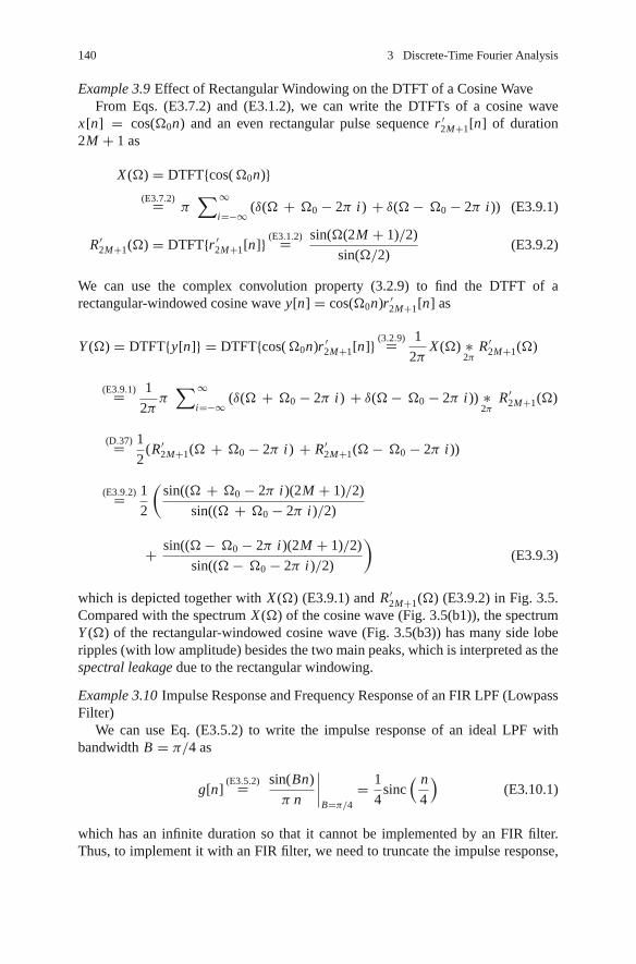
140 3 Discrete-Time Fourier Analysis
Example 3.9 Effect of Rectangular Windowing on the DTFT of a Cosine WaveFrom Eqs. (E3.7.2) and (E3.1.2), we can write the DTFTs of a cosine wave
x[n] = cos(Ω0n) and an even rectangular pulse sequence r ′2M+1[n] of duration
2M + 1 as
X (Ω) = DTFT{cos( Ω0n)}(E3.7.2)= π
∑∞i=−∞ (δ(Ω + Ω0 − 2π i) + δ(Ω − Ω0 − 2π i)) (E3.9.1)
R′2M+1(Ω) = DTFT{r ′
2M+1[n]} (E3.1.2)= sin(Ω(2M + 1)/2)
sin(Ω/2)(E3.9.2)
We can use the complex convolution property (3.2.9) to find the DTFT of arectangular-windowed cosine wave y[n] = cos(Ω0n)r ′
2M+1[n] as
Y (Ω) = DTFT{y[n]} = DTFT{cos( Ω0n)r ′2M+1[n]} (3.2.9)= 1
2πX (Ω) ∗
2πR′
2M+1(Ω)
(E3.9.1)= 1
2ππ
∑∞i=−∞ (δ(Ω + Ω0 − 2π i) + δ(Ω − Ω0 − 2π i)) ∗
2πR′
2M+1(Ω)
(D.37)= 1
2(R′
2M+1(Ω + Ω0 − 2π i) + R′2M+1(Ω − Ω0 − 2π i))
(E3.9.2)= 1
2
(sin((Ω + Ω0 − 2π i)(2M + 1)/2)
sin((Ω + Ω0 − 2π i)/2)
+ sin((Ω − Ω0 − 2π i)(2M + 1)/2)
sin((Ω − Ω0 − 2π i)/2)
)(E3.9.3)
which is depicted together with X (Ω) (E3.9.1) and R′2M+1(Ω) (E3.9.2) in Fig. 3.5.
Compared with the spectrum X (Ω) of the cosine wave (Fig. 3.5(b1)), the spectrumY (Ω) of the rectangular-windowed cosine wave (Fig. 3.5(b3)) has many side loberipples (with low amplitude) besides the two main peaks, which is interpreted as thespectral leakage due to the rectangular windowing.
Example 3.10 Impulse Response and Frequency Response of an FIR LPF (LowpassFilter)
We can use Eq. (E3.5.2) to write the impulse response of an ideal LPF withbandwidth B = π/4 as
g[n](E3.5.2)= sin(Bn)
π n
∣∣∣∣B=π/4
= 1
4sinc
( n
4
)(E3.10.1)
which has an infinite duration so that it cannot be implemented by an FIR filter.Thus, to implement it with an FIR filter, we need to truncate the impulse response,
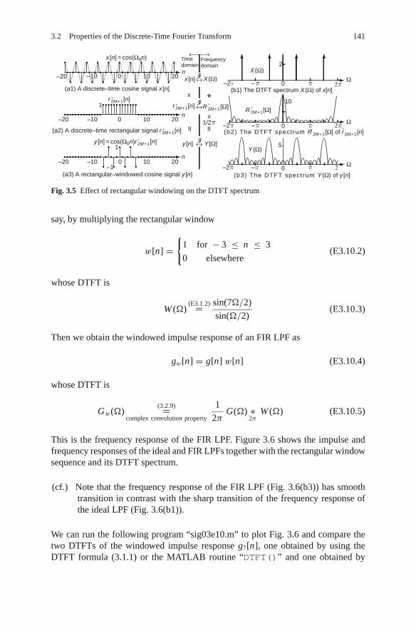
3.2 Properties of the Discrete-Time Fourier Transform 141
(a1) A discrete–time cosine signal x [n]
(a2) A discrete–time rectangular signal r2M+1[n]
(a3) A rectangular–windowed cosine signal y [n]
(b1) The DTFT spectrum X (Ω) of x[n]
y [n] = cos(Ω0n)r2M+1[n]
x [n] = cos(Ω0n)
0 20
Timedomain
Frequencydomain
↔
↔
–20 –10 0
1
10
x
x1/2π
–2π – π 0
2
π 2π
–2π – π 0
10
π 2π
–2π –π 0 π 2⎯
II II
*
20
–20 –10–1
0
1
10 20
n
n
n
'
'r2M+1[n]'r2M+1[n] ' 'R2M+1[Ω] R2M+1[Ω]
↔x [n]
y [n] Y [Ω]
X (Ω)X (Ω) Ω
Ω
Ω
(b2) The DTFT spectrum R2M+1[Ω] of r2M+1[n]
(b3) The DTFT spectrum Y (Ω) of y [n]
Y (Ω)5
' '
–20 10–10
'
F
F
F
Fig. 3.5 Effect of rectangular windowing on the DTFT spectrum
say, by multiplying the rectangular window
w[n] ={
1 for − 3 ≤ n ≤ 3
0 elsewhere(E3.10.2)
whose DTFT is
W (Ω)(E3.1.2)= sin(7Ω/2)
sin(Ω/2)(E3.10.3)
Then we obtain the windowed impulse response of an FIR LPF as
gw[n] = g[n] w[n] (E3.10.4)
whose DTFT is
Gw(Ω)(3.2.9)=
complex convolution property
1
2πG(Ω) ∗
2πW (Ω) (E3.10.5)
This is the frequency response of the FIR LPF. Figure 3.6 shows the impulse andfrequency responses of the ideal and FIR LPFs together with the rectangular windowsequence and its DTFT spectrum.
(cf.) Note that the frequency response of the FIR LPF (Fig. 3.6(b3)) has smoothtransition in contrast with the sharp transition of the frequency response ofthe ideal LPF (Fig. 3.6(b1)).
We can run the following program “sig03e10.m” to plot Fig. 3.6 and compare thetwo DTFTs of the windowed impulse response g7[n], one obtained by using theDTFT formula (3.1.1) or the MATLAB routine “DTFT()” and one obtained by

142 3 Discrete-Time Fourier Analysis
0.25Timedomain
Frequency domain
0.25
(a1) Ideal LPF impulse response (b1) Ideal LPF frequency response
(a2) Rectangular window sequence
(a3) FIR LPF impulse response
–10 –2π
1/2π
1
2π
G (Ω)
G (Ω)
Ω–π π0
B=π/4
0 10
–10 0
1
10
n
g [n]
g [n]
w [n ]
w [n ]
gw[n] gw[n]
n
–10 0 10n
(b2) Spectrum of rectangular window
(b3) FIR LPF frequency response
–2π 2π
W (Ω)
W (Ω)
Gw(Ω)Gw(Ω)
Ω–π π0
6
–2π 2π Ω–π π0
1
×
×
∗
π/4
F
F
F
Fig. 3.6 Effect of windowing on the spectrum or frequency response
using the circular convolution (E3.10.5) or the MATLAB routine“conv circular()”.
%sig03e10.m% Fig. 3.6: Windowing Effect on Impulse/Frequency Response of an ideal LPFclear, clfn= [-20: 20]; g= sinc(n/4)/4;N=400; f=[-400:400]/N +1e-10; W=2∗pi∗f;global P DD=pi/2; P=2∗pi; G=rectangular wave(W);subplot(321), stem(n,g,’.’), subplot(322), plot(f,G)M=3; wdw= [zeros(1,20-M) ones(1,2∗M+1) zeros(1,20-M)];Wdw= DTFT(wdw,W,-20); % DTFT Wdw(W) of wdw[n] - Appendix E for DTFTWdw t= sin(W∗(2∗M+1)/2)./sin(W/2); % Eq.(E3.1.2)discrepancy between DTFT and E3 1 2 = norm(Wdw-Wdw t)subplot(323), stem(n,wdw,’.’), subplot(324), plot(f,real(Wdw))gw= g.∗wdw;Gw= DTFT(gw,W,n(1)); % DTFT spectrum Gw(W) of gw[n]Gw 1P= conv circular(G,Wdw,N);discrepancy between circonv and DTFT= norm(Gw(1:N)-Gw 1P)/norm(Gw 1P)subplot(325), stem(n,gw,’.’)subplot(326), plot(f,real(Gw)), hold onplot(f(1:N),real(Gw 1P),’r’)
function z=conv circular(x,y,N)% Circular convolution z(n)= (1/N) sum m=0ˆN-1 x(m)∗y(n-m)if nargin<3, N=min(length(x),length(y)); endx=x(1:N); y=y(1:N); y circulated= fliplr(y);for n=1:N
y circulated= [y circulated(N) y circulated(1:N-1)];z(n)= x∗y circulated’/N;
end

3.2 Properties of the Discrete-Time Fourier Transform 143
3.2.7 Differencing and Summation in Time
As with the differentiation and integration property of the CTFT, the DTFT has thefollowing differencing and summation properties:
x[n] − x[n − 1]F↔ (1 − e− j Ω) X (Ω) (3.2.10)∑ n
m=−∞ x[m] = x[n] ∗ us[n]F↔
1
1 − e− j ΩX (Ω) + π X (0)
∑∞i=−∞ δ(Ω − 2π i) (3.2.11)
3.2.8 Frequency Differentiation
By differentiating both sides of the DTFT formula (3.1.1) w.r.t. Ω, we obtain
d X (Ω)
dΩ
(3.1.1)= −∑∞
n=−∞ j n x[n] e− j Ωn
which yields the frequency-differentiation property of the DTFT as
n x[n]F↔ j
d X (Ω)
dΩ(3.2.12)
This means that multiplication by n in the time domain results in differentiationw.r.t. Ω and multiplication by j in the frequency domain.
3.2.9 Time and Frequency Scaling
In the continuous-time case, we have Eq. (2.5.21) as
x(at)F↔ 1
| a | X(ω
a
)
However, it is not so simple to define x[an] because of the following reasons:
- If a is not an integer, say, a = 0.5, then x[0.5 n]|n=1 = x[0.5] is indeterminate.- If a is an integer, say, a = 2, then it does not merely speed up x[n], but takes the
even-indexed samples of x[n].
Thus we define a time-scaled version of x[n] as
x(K )[n] ={
x[n/K ] for n = Kr (a multiple of K ) with some integer r
0 elsewhere(3.2.13)

144 3 Discrete-Time Fourier Analysis
which is obtained by placing (K − 1) zeros between successive samples of x[n].Then we apply the DTFT formula (3.1.1) to get
X (K )(Ω)(3.1.1)=
∑∞n=−∞ x(K ) [n]e− j Ωn (3.2.13)=
with n=K r
∑∞r=−∞ x[r ] e− j ΩK r = X (KΩ)
(3.2.14)
3.2.10 Parseval’s Relation (Rayleigh Theorem)
If x[n] has finite energy and the DTFT X (Ω) = F{x[n]}, then we have
∑∞n=−∞ |x[n]|2 = 1
2π
∫2π
|X (Ω)|2d Ω (3.2.15)
where |X (Ω)|2 is called the energy-density spectrum of the signal x[n].
3.3 Polar Representation and Graphical Plot of DTFT
Similarly to the continuous-time case, we can write the polar representation of theDTFT as
X (Ω) = |X (Ω)|∠X (Ω)
If x[n] is real, then its DTFT X (Ω) = F{x[n]} has the following properties:
- X (Ω) is periodic with period 2π in Ω.- The magnitude |X (Ω)| is an even function of Ω and is symmetric about Ω = mπ
(m: an integer).- The phase ∠X (Ω) is an odd function of Ω and is anti-symmetric about Ω = mπ
(m: an integer).
Note that all the information about the DTFT of a real-valued sequence is containedin the frequency range [0, π ] since the portion for other ranges can be determinedfrom that for [0, π ] using symmetry and periodicity. Consequently, we usually plotthe spectrum for 0 ≤ Ω ≤ π only.
Remark 3.3 Phase Jumps in the DTFT Phase SpectrumFrom the phase spectra shown in Fig. 3.1(c1)–(c2) and 3.7(c1)–(c2), it can be
observed that there are two occasions for which the phase spectrum has discontinu-ities or jumps:
- A jump of ±2π occurs to maintain the phase value within the principal range of[−π,+π ].
- A jump of ±π occurs when the sign of X (Ω) changes.

3.3 Polar Representation and Graphical Plot of DTFT 145
The sign of phase jump is chosen in such a way that the resulting phase spectrumis odd or antisymmetric and lies in the principal range [−π,+π ] afterthe jump.
Remark 3.4 The DTFT Magnitude/Phase Spectra of Symmetric Sequences
(1) Especially for anti-symmetric sequences, their magnitude spectrum is zero atΩ = 0 (see Fig. 3.7(b1)–(b2)). This implies that the DC gain of digital filtershaving an anti-symmetric impulse response is zero so that they cannot be usedas a lowpass filter.
(2) As for the sequences that are even/odd about some point, their DTFTs havelinear phase −MΩ (proportional to the frequency) except for the phase jumpsso that the DTFT phase spectra are piecewise linear. Also, symmetric/anti-symmetric sequences, that are just shifted versions of even/odd ones, preservelinear phase because shifting does not impair the linear phase characteristic(see Eq. (3.2.6)). This is illustrated by Examples 3.1, 3.11, and 3.12 and will berestated in Remark 4.8, Sect. 4.6.
Example 3.11 DTFT of an Odd SequenceFor an odd sequence
n=x1[n] = · · · −4
0−31
−22
−11
00
1−1
2−2
3−1
40
50 · · · (E3.11.1)
(a1) An odd sequence (a2) An anti–symmetric sequence
(b1) The CTFT/DTFT magnitude spectra of x1(t ) /x1[n] (b2) The DTFT magnitude spectrum of x2[n]
(c1) The DTFT phase spectrum of x1[n] (c2) The DTFT phase spectrum of x2[n]
x1(t )x2[n ]
2
1 3t
–1–2
0
1x1[n ] = x1(nT) |T = 1
2
–5 50 5
6 6
t
–2
–2π 2π
π/2
0–π π –2π 2π0–π π
π
DTFT CTFT/T
T
X1(Ω)
∠X1(Ω) ∠X2(Ω)
| |
| | X2(Ω)| |X1(ω)
ω=Ω
Ω Ω
Ω Ω
| |
T
–2π–π/2
–π π 2π0 –2π –π
–π
π 2π0
Fig. 3.7 The DTFT spectra of an odd sequence and an anti-symmetric sequence

146 3 Discrete-Time Fourier Analysis
we have its DTFT as
X1(Ω) =∑∞
n=−∞ x1[n] e− j Ωn
= e j3Ω − e− j3Ω + 2(e j2Ω − e− j2Ω) + e j Ω − e− j Ω (D.22)= j2 sin(3Ω)
+ j4 sin(2Ω) + j2 sin(Ω)(D.12)= 4 sin(2Ω) (1 + cos Ω) e jπ/2 (E3.11.2)
Noting that the continuous-time version of this sequence is apparently the sum oftwo opposite-sign shifted triangular pulses, we can compute its CTFT spectrum as
x1(t) = 2(λD(t + 2) − λD(t − 2))(E2.3.4) with A=2,D=2↔
(2.5.6) with t1=2
X1(ω) = 4 sinc2(ω
π
)(e j2ω − e− j2ω) = j8 sin(2ω) sinc2
(ω
π
)(E3.11.3)
This sequence and its DTFT magnitude/phase spectra are depicted in Fig. 3.7(a1)and (b1)/(c1), respectively. The CTFT magnitude spectrum (E3.11.3) (divided bysampling interval or period T ) is plotted (in a dotted line) together with the DTFTmagnitude spectrum in Fig. 3.7(b1) for comparison.
Example 3.12 DTFT of an Anti-Symmetric SequenceFor the sequence which is anti-symmetric about n = 1.5
n = −2 −1 0 1 2 3 4 5x2[n] = · · · 0 0 −1 2 −2 1 0 0 · · · (E3.12.1)
we have its DTFT as
X2(Ω) =∑∞
n=−∞ x2[n] e− j Ωn = −1 + 2 e− j Ω − 2e− j2Ω + e− j3Ω
= −(1 − e− j3Ω) + 2(e− j Ω − e− j2Ω)
= −e− j3Ω/2(e j3Ω/2 − e− j3Ω/2) + 2e− j3Ω/2(e j Ω/2 − e− j Ω/2)
(D.22)= 2 j e− j3Ω/2
(2 sin
(Ω
2
)− sin
(3Ω
2
))
= 2
(2 sin
(Ω
2
)− sin
(3Ω
2
))∠(
−3Ω
2+ π
2
)(E3.12.2)
This sequence and its magnitude/phase spectra are depicted in Fig. 3.7(a2) and (b2)/(c2), respectively.

3.4 Discrete Fourier Transform (DFT) 147
3.4 Discrete Fourier Transform (DFT)
Before going into the DFT, let us consider the computational difference betweenthe CTFS or CTFT for a periodic or an aperiodic continuous-time function x(t) andthe DTFT for the discrete-time sequence x[n] consisting of the samples of x(t).Since the CTFS (2.1.5b) and CTFT (2.2.1a) involving a continuous-time integralcan be computed analytically for only x(t) described by some basic functions andrequire a numerical integration method for general finite-duration time functions,they are not practical when we need to find the spectra of real-world signals. TheDTFT (3.1.1) is computationally advantageous over the CTFS or CTFT since it doesnot involve any continuous-time integration. However, it can be computed, say, byusing the MATLAB routine “DTFT()”, only for finite-duration sequences unlessthe sequence is expressed by some basic sequences such as an exponential or sincone. Therefore in practice, signals are truncated in various ways to obtain a set offinite number of samples [S-2]:
- A transient signal is assumed to be zero after it decays to a negligible amplitude.- A periodic signal is sampled over an integral number of periods.- A random signal is multiplied by a “window” of finite duration (short-time
Fourier transform).
In any case, suppose we have a causal, finite-duration sequence x[n] containing Msamples. Then the DTFT formula (3.1.1) becomes
X (Ω) = X [e j Ω] = F{x[n]} =∑N−1
n=0x[n]e− j Ωn (3.4.1)
where N is set to be greater than or equal to M (the number of samples). Althoughit is easier to compute than the CTFS, CTFT, or the original DTFT, it may stillannoy the computer because the frequency Ω takes continuous values for all thatit is conventionally called the “digital” frequency. That is why we define and useanother Fourier technique, called the N -point DFT (discrete Fourier transform), asfollows:
X (k) = DFTN {x[n]} =∑N−1
n=0x[n]e− j2πk n/N =
∑N−1
n=0x[n]W k n
N (3.4.2)
with WN = e− j2π/N for k = 0 : N − 1
This is an N -point discrete-frequency sequence obtained by sampling one period ofthe finite version of DTFT, Eq. (3.4.1), conventionally at
Ω = kΩ0 = k2π
Nfor 0 ≤ k ≤ N − 1
where N is called the DFT size and Ω0 = 2π/N the digital fundamental or res-olution frequency just like ω0 = 2π/P in the CTFS. Note that these N frequency

148 3 Discrete-Time Fourier Analysis
points are equally-spaced over the digital frequency range [0, 2π ) (excluding theupperbound 2π). Also we can write the IDFT (inverse discrete Fourier transform)formula as
x[n] = IDFTN {X (k)} = 1
N
∑N−1
k=0X (k) e j2πk n/N
= 1
N
∑N−1
k=0X (k)W −k n
N for n = 0 : N − 1 (3.4.3)
Here, by substituting Eq. (3.4.2) into Eq. (3.4.3), we are going to demonstrate thevalidity of the IDFT formula, which amounts to verifying that the set of DFT sam-ples {X (k), k = 0 : N − 1} conveys all the information contained in the set oftime-domain samples {x[n], n = 0 : N − 1}, that is, x[n] can be recovered perfectlyfrom X (k):
x[n]?=
(3.4.3)
1
N
∑N−1
k=0X (k) W −k n
N(3.4.2)= 1
N
∑N−1
k=0
∑N−1
m=0x[m] W k m
N W −k nN
=∑N−1
m=0x[m]
(1
N
∑N−1
k=0W k(m−n)
N
)
=∑N−1
m=0x[m]δ[(m − n) mod N ]
O.K.= x[n]
(a mod b or a modulo b : the remainder after division of a by b)
where we have used the fact that
1
N
∑N−1
k=0W k(m−n)
N = 1
N
∑N−1
k=0e− j2πk(m−n)/N
={
1 if m − n = i N ( i : an integer)
0 otherwise(3.4.4)
There are two observations about the DFT pair (3.4.2) and (3.4.3):
- The DFT sequence X (k) is periodic in k with period N :
X (k + m N )(3.4.2)=
∑N−1
n=0x[n] e− j2π (k+m N ) n/N
=∑N−1
n=0x[n] e− j2πk n/N e− j2πm n (3.4.2)= X (k) (3.4.5)

3.4 Discrete Fourier Transform (DFT) 149
- The IDFT sequence x[n] is periodic in n with period N :
x [n + m N ](3.4.3)= 1
N
∑N−1
k=0X (k) e j2πk(n+m N )/N
= 1
N
∑N−1
k=0X (k) e j2πk n/N e j 2πk m (3.4.3)= x[n] (3.4.6)
The first observation (3.4.5) is no wonder since the DFT X (k) inherits the periodicityof the DTFT X (Ω) as X (k) originates from the samples of X (Ω) over its period. Incontrast, the second observation is very surprising since there is no reason to believethat any sequence x[n] is periodic and that with period equal to the DFT size N ,which can be arbitrarily chosen as long as it covers the duration of x[n]. Becauseof this illusory periodicity, the shift involved with the time shifting property and theconvolution related with the real convolution property of the DFT turn out to benot linear, but circular as will be discussed subsequently in Sects. 3.4.1 and 3.4.2.This headache is a kind of cost that we should pay in return for the computationalconvenience of DFT, which is discrete in both time and frequency so that it needsonly multiplication and summation instead of integration. If only the sequence x[n]is really periodic with period N , the DFT is a perfect Fourier technique for analyzingthe frequency characteristic and thus it might well be referred to as the discrete-timeFourier series (DTFS). In this context, when we want to emphasize the periodicityof DFT, we call it DFS (discrete Fourier series) pair and write the DFS pair as
X (k) = DFSN {x [n]} =∑N−1
n=0x[n] e− j 2πk n/N =
∑N−1
n=0x[n] W kn
N (3.4.7)
x [n] = IDFSN {X (k)} = 1
N
∑N−1
k=0X (k) e j 2πk n/N = 1
N
∑N−1
k=0X (k) W − k n
N
(3.4.8)
3.4.1 Properties of the DFT
The DFT has properties similar to those of the CTFS such as the real convolutionproperty (2.5.13) since the DFT regards a time-domain sample sequence x[n] as oneperiod of its periodic extension (with period equal to the DFT size N ) that can bedescribed by
x [n] = xN [n] rN [n] (3.4.9)
where xN [n] is the periodic extension of x[n] with period N and rN [n] the rectan-gular pulse sequence with duration of n = 0 : N − 1:
x [n] =∑∞
m=−∞ x[n + m N ] = x [n mod N ] (3.4.10a)
rN [n] = us[n] − us[n − N ] ={
1 for 0 ≤ n ≤ N − 1
0 elsewhere(3.4.10b)

150 3 Discrete-Time Fourier Analysis
On the other hand, the DFT sequence is born from the samples of the DTFT andthus it inherits most of the DTFT properties except that the real translation andconvolution in the time domain are not linear, but circular as with the CTFS. There-fore we discuss only the two properties and summarize all the DFT properties inAppendix B.
3.4.1.1 Real/Complex Translation – Circular Shift in Time/Frequency
Figure 3.8(a), (b1), (b2), and (d) show a sequence x[n] of finite duration N = 4, itsperiodic extension xN [n], its shifted version xN [n−M] (M = 2), and its rectangular-windowed version xN [n − M]rN [n], respectively. You can see more clearly fromFig. 3.8(a), (c1), (c2), and (d) that xN [n − M]rN [n] is the circular-shifted (rotated)version of x[n] where Fig. 3.8(c1) and (c2) show the circular representation of thefinite-duration sequence x[n] and its shifted or rotated version displayed around thecircle with a circumference of N points. With this visual concept of circular shift,we can write the (circular) time-shifting property of DFS and DFT as
xN [n − M] (circular shift)DFS↔ W Mk
N X (k) (3.4.11a)
xN [n − M]rN [n] (one period of circular shift)DFT↔ W Mk
N X (k) (3.4.11b)
We can also apply the duality between the time and frequency domains to writethe (circular) frequency-shifting property of DFS/DFT:
W −LnN xN [n]
DFS↔ X (k − L) (circular shift) (3.4.12a)
W −LnN x[n]
DFT↔ X (k − L)rN [k] (one period of circular shift) (3.4.12b)
x [n ]
nn = 2
n = 2
n = 1
n = 1
n = 0
n = 0
n = N –1
n = N –1n
n n
xN [n ]
N –10
Periodic repetition
Circular representation
Linear representation
Taking one period(Rectangular windowing)
Circular shift
Linear shift
(a) (c1)
(c2)
(d)
(b1)
(b2)
1
N –10 1
N –10 1N –10 1
~
xN [n –2 ]~ xN [n –2 ] rN [n ]~
Fig. 3.8 Circular shift of a sequence by 2 samples

3.4 Discrete Fourier Transform (DFT) 151
3.4.1.2 Real/Complex Convolution – Circular Convolutionin Time/Frequency
Let us consider two sequences x[n] and y[n], both of duration M ≤ N and eachwith DFT X (k) and Y (k), respectively. Also let us denote the periodic extensions ofthe two sequences and their DFSs by x[n], y[n], X (k), and Y (k), respectively. Thenwe can write the product of the two DFSs X (k) and Y (k) as
X (k) = DFSN {x [n]} =∑N−1
m=0x[m] W km
N
Y (k) = DFSN {y [n]} =∑N−1
r=0y [r ] W kr
N
; X (k)Y (k) =∑N−1
m =0
∑N−1
r=0x[m] y [r ] W k(m+r )
N (3.4.13)
and compute its IDFS (inverse discrete Fourier series) as
IDFSN{
X (k)Y (k)} (3.4.8)= 1
N
∑N−1
k=0X (k)Y (k) W −k n
N
(3.4.13)=∑N−1
m=0x[m]
∑N−1
r=0y [r ]
(1
N
∑N−1
k=0W k(r−n+m)
N
)
(3.4.4)=∑N−1
m=0x[m]
∑N−1
r=0y [r ]δ[r − (n − m)]
(1.1.32)=∑N−1
m =0x[m] y [n − m] = x[n] ∗
Ny [n] (3.4.14)
where ∗N
denotes the circular or periodic convolution sum with period N . This
implies the real convolution property of DFS/DFT as
x[n] ∗N
y [n] (circular convolution)DFS↔ X (k)Y (k) (3.4.15a)
(x[n] ∗N
y [n]) rN [n] (one period of circular convolution)DFT↔ X (k) Y (k) (3.4.15b)
In duality with this, we can interchange the time and frequency indices to write thecomplex convolution property as
x[n] y [n]DFS↔ 1
N
∑N−1
i=0X (i)Y (k − i) = 1
NX (k) ∗
NY (k) (circular convolution)
(3.4.16a)
x[n] y [n]DFT↔ 1
N
(X (k) ∗
NY (k)
)rN [k] (one period of circular convolution)
(3.4.16b)

152 3 Discrete-Time Fourier Analysis
Note that the shift of a periodic sequence along the time/frequency axis actuallycauses a rotation, making the sequence values appear to wrap around from thebeginning of the sequence to the end.
3.4.2 Linear Convolution with DFT
As discussed in the previous section, circular translation/convolution is natural withthe DFT/DFS. However, in most applications of digital signal processing, linearconvolution is necessary. As will be seen later, very efficient algorithms called FFTare available for computing the DFT of a finite-duration sequence. For this reason,it can be computationally advantageous to use the FFT algorithm for computing aconvolution in such a way that the linear convolution corresponds to a single periodof a circular convolution.
Specifically, suppose the signals x[n] and y[n] are of finite duration Nx and Ny ,and defined on n = 0 : Nx − 1 and on n = 0 : Ny − 1, respectively. Then, theprocedure for computing the linear convolution z[n] = x[n] ∗ y[n] is as below (seeFig. 3.9):
0) Extend the given sequences x[n] and y[n] to the duration of N ≥ Nx + Ny − 1by zero-padding where Nx + Ny − 1 is the expected length of the linearconvolution of the two sequences (see Remark 1.5(1)).(cf.) Zero-padding a sequence means appending zeros to the end of the
sequence.)1) Compute X (k) = DFTN {x[n]} and Y (k) = DFTN {y[n]}. (3.4.17a)2) Multiply the two DFT sequences Z (k) = X (k)Y (k)
for k = 0 : N − 1. (3.4.17b)3) Compute z[n] = IDFTN {Z (k)} where z[n] = x[n] ∗ y[n]. (3.4.17c)
Example 3.13 Linear Convolution Using the DFTWe want to find the linear convolution z[n] = x[n] ∗ y[n] of the two sequences
depicted in Fig. 3.10(a), where
x[n] =
⎧⎪⎨⎪⎩
1 for n = 0
0.5 for n = 1
0 elsewhere
and y[n] =
⎧⎪⎨⎪⎩
0.5 for n = 0
1 for n = 1
0 elsewhere
(E3.13.1)
Zero-paddingto duration N
Zero-paddingto duration N
N – pointDFT
N ≥ Nx + Ny – 1
N – pointDFT
N – pointDFT
X(k) = DFTN {x [n]}
Y(k) = DFTN {y [n]}
x [n]
z [n]
y [n]
length Ny
Z(k) = X(k)Y(k)length Nx
Fig. 3.9 Linear convolution using the DFT

3.4 Discrete Fourier Transform (DFT) 153
(a) Time-domain approach (Fig. 3.10(a))
z[n] = 0 for n < 0 or n ≥ 3(= Nx + Ny − 1 = 2 + 2 − 1)
z[0] = x [0] y[0] + x[1] y[−1] = 0.5
z[1] = x [0] y[1] + x[1] y[0] = 1.25 (E3.13.2)
z[2] = x [0] y[2] + x[1] y[1] = 0.5
z[3] = x [0] y[3] + x[1] y[2] = 0
(b) Frequency-domain approach with 2-point DFT (Fig. 3.10(b))We can use the DFT formula (3.4.2) with N = 2 to get the DFTs of the twosequences as
X2(k) = ∑2−1n=0 x[n]e− j2πkn/2 = 1 + 0.5(−1)k = 1.5, 0.5 for k = 0, 1
Y2(k) = ∑2−1n=0 y[n]e− j2πkn/2 = 0.5 + (−1)k = 1.5, −0.5 for k = 0, 1
so that
Z2(k) = X2(k) Y2(k) = 2.25, −0.25 for k = 0, 1 (E3.13.3)
Then we use the IDFT formula (3.4.3) to get
z2[n] = 1
2
∑2−1
k=0Z2(k)e j2πkn/2
= 1
2
(Z2(0) + (−1)n Z2(1)
) = 1, 1.25 for n = 0, 1 (E3.13.4)
(a) Linear convolution (b) Circular convolution with 2-point DFT (c) Circular convolution with 3-point DFT
0.5
x2 [n ]
n–5 –4 –3 –2 –1 0 1 2 3 4 5 6 7
1
∼
0.5
n–5 –4 –3 –2 –1 0 1 2 3 4 5 6 7
1y2 [n ]∼
0
0.5
x [n ]
n1
1
z [n ] = x [n ]∗y [n ]
n0
0.5
1.25
1 2
0.5
y [n ]
n0 1
1
1.25
n–5 –4 –3 –2 –1 0 1 2 3 4 5 6 7
1
z2 [n ]∼
0.5
n
1x3 [n ]∼
–5 –4 –3 –2 –1 0 1 2 3 4 5 6 7
0.5
n
1y3 [n ]∼
–5 –4 –3 –2 –1 0 1 2 3 4 5 6 7
n2
1.25
0.5 0.5
z3 [n ]∼
–5 –4 –3 –2 –1 0 1 3 4 5 6 7
Fig. 3.10 Linear and circular convolutions with DFT

154 3 Discrete-Time Fourier Analysis
This corresponds to one period of the periodic extension of z[n] (obtained in part(a)) with period N = 2 and is not equal to z[n]. This illustrates that time-aliasingeffect might occur if the DFT size N is not sufficiently large.
(c) Frequency-domain approach with 3-point DFT (Fig. 3.10(c))We can use the DFT formula (3.4.2) with N = 3 to get the DFTs of the twosequences as
X3(k) =∑3−1
n=0x[n]e− j2πkn/3 = 1 + 0.5e− j2πk/3
= 1.5, 1 + 0.5e− j2π/3, 1 + 0.5e− j4π/3 for k = 0, 1, 2
Y3(k) =∑3−1
n=0y[n]e− j2πkn/3 = 0.5 + e− j2πk/3
= 1.5, 0.5 + e− j2π/3, 0.5 + e− j4π/3 for k = 0, 1, 2
so that
Z3(k) = X3(k)Y3(k) = 0.5 + 1.25e− j2πk/3 + 0.5e− j4πk/3 (E3.13.5)
We can match this with the IDFT formula (3.4.3) to get
z3[n] = 0.5, 1.25, 0.5 for n = 0, 1, 2 (E3.13.6)
This agrees with the linear convolution z[n] obtained in part (a) for n = 0 ∼ 2.(d) MATLAB Program
We can run the following program “sig03e13.m” to apply the above procedureto get the linear convolution using the DFT. Note the following:
- The built-in MATLAB functions “fft(x,N)” and “ifft(X,N)” are usedto compute the N-point DFT X (k) = DFTN {x[n]} and IDFT x[n] =IDFTN {X (k)}, respectively.
- Depending on whether the length of the sequence given as the first inputargument of “fft(x,N)” or “ifft(X,N)” is less or greater than the sec-ond input argument N, the sequence will be zero-padded or truncated so thatits resulting length will be N.
- Note that, to exploit the computational efficiency of FFT (fast Fourier trans-form), the DFT size N should be chosen as a power of two greater than orequal to the length of the sequence.
%sig03e13.m% Use 2-point/3-point DFT for computing a (linear) convolutionclear, clfx= [1 0.5]; y= [0.5 1];z= conv(x,y) % Linear convolutionN= 3; % DFT size

3.4 Discrete Fourier Transform (DFT) 155
XN= fft(x,N); YN=fft(y,N);ZN= XN.∗YN;zN= ifft(ZN) % Circular convolution expected to agree with the linear one% Sometimes, you had better take the real part of IDFT result% by using real(ifft(ZN)) to make sure of its being real-valued.
(cf.) The above procedure, which is depicted in Fig. 3.9 and illustrated inExample 3.13, paves the way to use the DFT for computing the linearconvolution of two finite-duration sequences.
Remark 3.5 How to Choose the DFT Size N in Connection with Zero Padding
(1) In computing the DFT of a given sequence x[n] of length M , we are free tochoose the DFT size N , i.e., the number of sampled frequency points over[0, 2π ) (one period of digital frequency) as long as it is greater than or equal toM . Choosing N > M corresponds to increasing the length of x[n] by appendingit with additional zero-valued samples - padding with zeros. This procedurecalled zero padding may be used to fill out the sequence length so that anN = 2L -point FFT (fast Fourier transform) algorithm could be applied (seeSect. 3.6) or a linear convolution of two sequences could be performed with-out causing a time-aliasing problem (see Example 3.13). It can also be used toprovide a better-looking display of the frequency contents of a finite-durationsequence by decreasing the digital frequency spacing (resolution frequency)2π/N so that the discrete DFT spectrum X (k) can look close to the continuousDTFT spectrum X (Ω) (see Example 3.14).
(2) As can be seen from the DTFT formula (3.1.1), zero padding does not alter thecontinuous spectrum X (Ω), but just decreases the interval width between suc-cessive discrete frequencies in the DFT spectrum. However, when the signal isnot of finite duration, zero padding can lead to erroneous results. Conclusively,zero padding is justified only when a signal is of finite duration and has alreadybeen sampled over the entire range where it is nonzero.
3.4.3 DFT for Noncausal or Infinite-Duration Sequence
Let us consider the DFT formula (3.4.2):
X (k) = DFTN {x[n]} =∑N−1
n=0x[n]e− j2πkn/N for k = 0 : N − 1
This is defined for a causal, finite-duration sequence x[n] so that we can castit into a computer program without taking much heed of the negative indices.(C language prohibits using the negative indices for array and MATLAB does notaccept even zero index.) Then, how can we get the DFT spectrum of noncausal orinfinite-duration sequences? The answer is as follows:

156 3 Discrete-Time Fourier Analysis
- For a noncausal sequence, append the noncausal part to the end of the sequenceafter any necessary zero-padding is done so that the resulting sequence can becausal.
- For an infinite-duration sequence, set the time-duration [0, N − 1] so that themost significant part of the sequence can be covered. To increase the DFT size isalso helpful in making the DFT close to the DTFT. Compare Fig. 3.11(b2)/(c2)with (b3)/(c3). Also compare Fig. 3.12.1(b1) with Fig. 3.12.2(b1).
Example 3.14 DFT of a Non-causal Pulse SequenceConsider a sequence which is depicted in Fig. 3.11(a1). Shifting the noncausal
part x[−1] = 1/3 into the end of the sequence yields a causal sequence
xN [n] =⎧⎨⎩
1/3 for n = 0, 1, N − 1
0 elsewhere(E3.14.1)
where N is the DFT size. This corresponds to one period of the periodic extensionxN [n] (see Fig. 3.11(a2) with N = 4 and (a3) with N = 8).
Then we can compute the N -point DFT of xN [n] as
X N (k)(3.4.2)=
∑N−1
n=0xN [n]e− j2πkn/N = 1
3
n=0
e− j2πk0/N +1
3
n=1
e− j2πk1/N +1
3
n=N−1
e− j2πk(N−1)/N
= 1
3
(1 + e− j2πk/N + e− j2πk(N−1)/N
) = 1
3
(1 + e− j2πk/N + e j2πk/N
)= 1
3(1 + cos(2πk/N )) for k = 0 : N − 1 (E3.14.2)
00
1
0
–4 –1 0 1 3 4 5 7 8 9 –1 0 1 4 7 8 9
1/3 1/3 1/3
x [n] x4[n] x4[n]
(a1) A noncausal sequence
(b1) The DTFT magnitude spectrum
(c1) The DTFT phase spectrum (c2) The DFT phase spectrum (c3) The DFT phase spectrum
DTFT phase ∠X(Ω) 4-point DFT phase ∠X4(k) 8-point DFT phase ∠X8(k)
(b2) The DFT magnitude spectrum (b3) The DFT magnitude spectrum
(a2) Periodic extension with N = 4 and its one period
(a3) Periodic extension with N = 8 and its one period
–1 0 4n n n
1
0
1
DTFT magnitude
π 2π
–π –π –π
2πN
Ω1 2 3
k
X(Ω)
4-pointDFT magnitude
X4(k)
8-pointDFT magnitude
X8(k)
0 10
1
2πN
2 3 4 5 6 7k
0000
2ππ/3 2π/3 Ω
1 2 3k
0
10
2 3 4 5 6 7k
x8[n]x8[n]
Fig. 3.11 DTFT and DFT for a noncausal sequence

3.4 Discrete Fourier Transform (DFT) 157
Figure 3.11(b2)/(c2) and (b3)/(c3) show the magnitude/phase of this DFT withN = 4 and those with N = 8, respectively. Note the following:
- The overlapped DTFT spectra in dotted lines, obtained in Example 3.1 and plot-ted in Figs. 3.1 and 3.11(b1)/(c1), illustrate the fact that the DFT X N (k) are justthe samples of the DTFT X (Ω) at Ω = kΩ0 = 2πk/N for 0 ≤ k ≤ N − 1 aslong as the whole duration of the sequence is covered by [0 : N − 1].
- Figure 3.11(a2) and (a3) differ in the length of zero padding performed beforeappending the noncausal part to the end of the sequence. Comparing the corre-sponding DFT spectra in Figure 3.11(b2)/(c2) and (b3)/(c3), we see that longerzero-padding increases the DFT size and thus decreases the digital resolutionfrequency Ω0 = 2π/N so that the DFT looks closer to the DTFT.
Example 3.15 DFT of an Infinite-Duration SequenceConsider a real exponential sequence of infinite duration described by
x [n] = an us[n] ( |a| < 1 ) (E3.15.1)
This sequence is shown partially for n = 0 : 7 in Fig. 3.12.1(a1) and for n = 0 : 15in Fig. 3.12.2(a1).
(a) The DTFT of this infinite-duration sequence was obtained in Example 3.2 as
X (Ω)(E3.2.1)= 1
1 − a e− j Ω(E3.15.2)
Thus we get the samples of the DTFT at Ω = kΩ0 = 2πk/N as
00
(a1) A part of an infinite-duration sequence4 7
x [0:7 ]
n
1
(a2) Periodic extension of x [n ] with period N = 80 4 8 16
x 8[n]
n0
1 ~
0
⇒N = 8-point samples of DTFT
0 π 2πN2π
8-pointIDFT
Ω
(b2) Samples of the DTFT X(Ω) at Ω = 2πk /N
0
⇒
0
8-pointDFT
: DTFT magnitude X(Ω)4
4 7
(b1) The 8-point DFT X8(k ) and the DTFT X(Ω)
k
: DFT magnitude X8(k )
Fig. 3.12.1 Relationship between the 8-point DFT and the DTFT for an infinite-durationsequence

158 3 Discrete-Time Fourier Analysis
1
00 4
(a1) A part of an infinite-duration sequence (b1) The 16-point DFT X16 (k ) and the DTFT X (Ω)
(a2) Periodic extension of x [n ] with period N = 16 (b2) Samples of the DTFT X (Ω) at Ω = 2πk /N
8 15
x [0:15]
4
0
0
4
0
0
8 15n
1
00 8 16
n
k
: DTFT magnitude X(Ω): DFT magnitude X16(k )
x 16[n ]~ N=16-point samples of DTFT
π 2πΩ
16-pointDFT
16-pointIDFT
2πN
Fig. 3.12.2 Relationship between the 16-point DFT and the DTFT for an infinite-durationsequence
X (kΩ0)(E3.15.2)= 1
1 − ae− jkΩ0= 1
1 − ae− j2πk/N
= 1
1 − aW kN
with WN = e− j2π/N (E3.15.3)
(b) We can use the DFT formula (3.4.2) to find the N -point DFT of x[n] for n =0 : N − 1:
X (k)(3.4.2)=
∑N−1
n=0x[n]W nk
N
(E3.15.1)=∑N−1
n=0an W nk
N = 1 − aN W k NN
1 − aW kN
= 1 − aN
1 − aW kN
for k = 0 : N − 1
(E3.15.4)
Comparing this with (E3.15.3) reveals the following:
- The DFT and the DTFT samples are not exactly the same for an infinite-duration sequence, while they conform with each other for a finite-durationsequence whose duration can somehow be covered in [0 : N − 1]
- Larger DFT size N will make the DFT closer to the sampled DTFT. This canalso be seen visually by comparing Figs. 3.12.1(b1) and 3.12.2(b1).
(c) One might wonder what the time-domain relationship between the DFT X (k)and the sampled DTFT X (kΩ0) is for the infinite-duration sequence. Thiscuriosity seduces us to find the IDFT of X (kΩ0) as
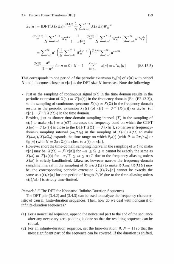
3.4 Discrete Fourier Transform (DFT) 159
xN [n] = IDFT{X (kΩ0)} (3.4.3)= 1
N
∑N−1
k=0X (kΩ0)W −kn
N
(E3.15.3)= 1
N
∑N−1
k=0W −kn
N
1
1 − aW kN
(D.23)= 1
N
∑N−1
k=0W −kn
N
{∑∞r=0
ar W krN
}
=∑∞
r=0ar
(1
N
∑N−1
k=0W k(r−n)
N
)(3.4.4)=
∑∞i=0
an+i N
(D.23)= an
1 − aNfor n = 0 : N − 1
N→∞→|a|<1
x[n] = anus[n] (E3.15.5)
This corresponds to one period of the periodic extension xN [n] of x[n] with periodN and it becomes closer to x[n] as the DFT size N increases. Note the following:
- Just as the sampling of continuous signal x(t) in the time domain results in theperiodic extension of X (ω) = F{x(t)} in the frequency domain (Eq. (E2.13.3)),so the sampling of continuous spectrum X (ω) or X (Ω) in the frequency domainresults in the periodic extension xP (t) (of x(t) = F−1{X (ω)}) or xN [n] (ofx[n] = F−1{X (Ω)}) in the time domain.
- Besides, just as shorter time-domain sampling interval (T ) in the sampling ofx(t) to make x[n] = x(nT ) increases the frequency band on which the CTFTX (ω) = F{x(t)} is close to the DTFT X (Ω) = F{x[n]}, so narrower frequency-domain sampling interval (ω0/Ω0) in the sampling of X (ω)/X (Ω) to makeX (kω0)/X (kΩ0) expands the time range on which xP (t) (with P = 2π/ω0) orxN [n] (with N = 2π/Ω0) is close to x(t) or x[n].
- However short the time-domain sampling interval in the sampling of x(t) to makex[n] may be, X (Ω) = F{x[n]} for −π ≤ Ω ≤ π cannot be exactly the same asX (ω) = F{x(t)} for −π/T ≤ ω ≤ π/T due to the frequency-aliasing unlessX (ω) is strictly bandlimited. Likewise, however narrow the frequency-domainsampling interval in the sampling of X (ω)/X (Ω) to make X (kω0)/X (kΩ0) maybe, the corresponding periodic extension xP (t)/xN [n] cannot be exactly thesame as x(t)/x[n] for one period of length P/N due to the time-aliasing unlessx(t)/x[n] is strictly time-limited.
Remark 3.6 The DFT for Noncausal/Infinite-Duration SequencesThe DFT pair (3.4.2) and (3.4.3) can be used to analyze the frequency character-
istic of causal, finite-duration sequences. Then, how do we deal with noncausal orinfinite-duration sequences?
(1) For a noncausal sequence, append the noncausal part to the end of the sequenceafter any necessary zero-padding is done so that the resulting sequence can becausal.
(2) For an infinite-duration sequence, set the time-duration [0, N − 1] so that themost significant part of the sequence can be covered. If the duration is shifted,

160 3 Discrete-Time Fourier Analysis
apply the time-shifting property to the DFT for obtaining the right phase spec-trum. You can also increase the DFT size to make the DFT close to the DTFT,which accommodates infinite-duration sequences.
3.5 Relationship Among CTFS, CTFT, DTFT, and DFT
3.5.1 Relationship Between CTFS and DFT/DFS
To investigate the relationship between CTFS and DFT/DFS, suppose we have acontinuous-time periodic signal xP (t) with period P and its discrete-time versionxN [n] = xP (nT ), which is obtained by sampling xP (t) at the rate of N times perperiod P . Since xP (t) is a continuous-time periodic signal with period P , we canuse Eq. (2.1.5a) to write its CTFS representation as
xP (t)(2.1.5a)= 1
P
∑∞k=−∞ Xk e jkω0t P =N T=
ω0=2π/P=2π/N T
1
N T
∑∞k=−∞ Xk e j2πkt/N T
(3.5.1)
Substituting t = nT into this equation and using the fact that e j2πkn/N is uniqueonly for n mod N yields
xP (nT )(3.5.1)= 1
N T
∑∞k=−∞ Xke j2πknT/N T = 1
N T
∑∞k=−∞ Xke j2πkn/N
(since e j2πkn/N is unique only for n mod N )
= 1
N T
∑N−1
k=0
∑∞m=−∞ Xk+m N e j 2π (k+m N )n/N
= 1
N
∑N−1
k=0
(1
T
∑∞m=−∞ Xk+m N
)e j 2πkn/N (3.5.2)
We can match this equation with the IDFS/IDFT formula (3.4.8)/(3.4.3) for xN [n] =xP (nT )
xN [n] = 1
N
∑N−1
k=0X N (k) e j 2πk n/N
to write the relation between the CTFS coefficients Xk of a periodic signal xP (t)(with period P = N T ) and the N -point DFT/DFS coefficients X N (k) of xN [n] =xP (nT ) as
X N (k) = 1
T
∑∞m=−∞ Xk+m N (3.5.3)
This implies that the DFT/DFS of xN [n] = xP (nT ) is qualitatively the periodicextension of the CTFS of xP (t) (with period N in frequency index k), i.e., thesum of infinitely many shifted version of CTFS. This explains how the DFT/DFS

3.5 Relationship Among CTFS, CTFT, DTFT, and DFT 161
strays from the CTFS because of frequency-aliasing unless the CTFS spectrumXk is strictly limited within the low-frequency band of (−(N/2)ω0, (N/2)ω0) =(−π/T, π/T ) where the DFT size N equals the number of samples per period Pand the fundamental frequency is ω0 = 2π/P = 2π/N T .
3.5.2 Relationship Between CTFT and DTFT
To investigate the relationship between CTFT and DTFT, suppose we have acontinuous-time signal x(t) and its discrete-time version x[n] = x(nT ). As a bridgebetween x(t) and x[n], let us consider the sampled version of x(t) with samplinginterval or period T as
x∗(t) = x(t)δT (t) (δT (t) =∑∞
n=−∞ δ(t − nT ) : the impulse train) (3.5.4)
Noting that x∗(t) is still a continuous-time signal, we can use Eq. (2.2.1a) to writeits CTFT as
X∗(ω)(2.2.1a)=
∫ ∞
−∞x∗(t)e− jωt dt
(3.5.4)=∫ ∞
−∞x(t)
∑∞n=−∞ δ(t − nT )e− jωt dt
=∑∞
n=−∞
∫ ∞
−∞x(t)e− jωtδ(t − nT ) dt
(1.1.25)=∑∞
n=−∞ x(nT )e− jωnT
=∑∞
n=−∞ x[n] e− jΩn∣∣Ω=ωT
(3.1.1)= Xd (Ω)|Ω=ωT (3.5.5)
This implies that Xd (Ω) = DTFT{x[n]} and X∗(ω) = CTFT{x∗(t)} are essentiallythe same and that Xd (Ω) can be obtained from X∗(ω) via a variable substitution ω =Ω/T . On the other hand, we recall from Eq. (E2.13.3) that X∗(ω) = CTFT{x∗(t)}is expressed in terms of X (ω) = CTFT{x(t)} as
X∗(ω)(E2.13.3)= 1
T
∑∞m=−∞ X (ω + mωs) with ωs = 2π
T(3.5.6)
Combining these two equations (3.5.5) and (3.5.6), we can write the relationbetween the CTFT and the DTFT as
Xd (Ω)(3.5.5)= X∗(ω)|ω=Ω/T
(3.5.6)= 1
T
∑∞m=−∞ X
(Ω
T+ m
2π
T
)(3.5.7)
where ω and Ω are called the analog and digital frequency, respectively.This implies that the DTFT of x[n] = x(nT ) is qualitatively the periodic
extension of the CTFT of x(t) (with period 2π/T in analog frequency ω or 2π
in digital frequency Ω), i.e., the sum of infinitely many shifted version of CTFT.This explains how the DTFT strays from the CTFT because of frequency-aliasing

162 3 Discrete-Time Fourier Analysis
unless the CTFT spectrum X (ω) is strictly limited within the low-frequency bandof (−π/T, π/T ) where T is the sampling interval of x[n] = x(nT ). Fig. 3.7(b1)illustrates the deviation of the DTFT spectrum from the CTFT spectrum caused byfrequency-aliasing.
3.5.3 Relationship Among CTFS, CTFT, DTFT, and DFT/DFS
As stated in Remark 2.7(2) and illustrated in Fig. 2.8, the CTFS Xk’s of a periodicfunction xP (t) are the samples of the CTFT X (ω) of the one-period function xP (t)at kω0 = 2πk/P:
Xk(2.2.4)= X (ω)|ω=kω0=2πk/P (3.5.8)
Likewise, as discussed in Sect. 3.4 and illustrated in Fig. 3.11, the DFT/DFS X (k)’sof a periodic sequence xP [n] are the samples of the DTFT Xd (Ω) of the one-periodsequence xP [n] at kΩ0 = 2πk/N :
X (k)(3.4.1)&(3.4.2)= Xd (Ω)|Ω=kΩ0=2πk/N (3.5.9)
Figure 3.13 shows the overall relationship among the CTFS, CTFT, DTFT, andDFT/DFS based on Eqs. (3.5.3), (3.5.7), (3.5.8), and (3.5.9). Figure 3.14 showsthe CTFT, DTFT, DFT/DFS, and CTFS spectra for a continuous-time/discrete-time rectangular pulse or wave, presenting us with a more specific view of theirrelationship. Some observations are summarized in the following remark:
Remark 3.7 Relationship among the CTFS, CTFT, DTFT, and DTFS (DFT/DFS)Figures 3.13 and 3.14 shows the overall relationship among the CTFS, CTFT,
DTFT, and DTFS (DFT/DFS) from a bird’s-eye point of view. The followingobservations and comparisons are made.
(1) Among the four Fourier spectra, the CTFS and CTFT are more desired thanthe DTFS and DTFT since all physical signals are continuous-time signals.
Time-domain periodic extension with period N
Time-domain periodic extension with period P
Frequency-domain periodic extension
Frequency-domain periodic extensionFrequency-domain
sampling
Frequency-domain sampling
DTFT DTFS (DFT/DFS)
CTFT CTFSTime-domain
samplingat t = nT
Time-domain samplingat t = nT
(2.2.1a)X(ω) = ∫–∞ x(t) e–j ωt dt
∞ (2.1.5b) = ∫p x(t )e–j 2πkt / P dt
at ω = kω0 = k 2πP
at Ω = kΩ0 = k 2πN
∞ 2πT
1T
Xd (Ω) = Σm = – ∞X(ω + m )⎮ω = Ω/T(3.5.6)
∞Xd (Ω) = Σn = – ∞ x [n]e–j Ωn(3.1.1)
∞1T
X (K) = Σm = – ∞Xk + mN
(3.5.3)
(3.4.2) N –1X (K) = Σn = 0 x [n]e–j 2πkn / N∼
∼Xk
Fig. 3.13 Overall relationship among the CTFT, CTFS, DTFT, and DTFS (DFT/DFS)

3.5 Relationship Among CTFS, CTFT, DTFT, and DFT 163
–10 100
–10 0 10
–8 0 8
T
(a0) A pulse signal x(t ) (b0) The CTFT spectrum X(ω) of x(t)
(b2) N = 8-point DFS/DFT spectrum X(k) of x8(n)
(b3) The CTFS spectrum Xk of x8(t )
(b4) The DTFT spectrum Xd (Ω) of x [n]
(b1) The DTFT spectrum Xd (Ω) of x[n](a1) x [n] obtained by sampling x (t ) with T = 1
(a2) x8[n] – a periodic extension of x [n] with period N = 8
–8 0 8(a3) x8(t) – a periodic extension of x (t ) with period p = 8
–20 0
T
20
N = 16Period
(a4) x (n) obtained by sampling x(t ) withT = 0.5
(a5) x16(n) – a periodic extension of x [n] with period N = 16
t
n
X(ω)
X(ω)
Xd (Ω)
Xd (Ω)
Xd (Ω)
Xd (Ω)
X(k)
Xk
X(k)
X(ω)
X(ω)
–4π –2π 2π
2π
0
N
4π–π π
n
t
n
n
N = 8Period
P = 8Period
ω
–4π –2π
–16 –8
2π0
0 8 16
–16
–2π 2π–π π
–8 0
0
8 16
–16 –8 0 8 16
4π–π πΩ
k
k
k
Ω
Ω0=
2πN
Ω0=
2πp
ω0=
∼
∼ ∼
∼∼
∼(b5) N = 16- point DFS/DFT spectrum X(k) of x16[n]
Fig. 3.14 Examples of CTFT, DTFT, DFS/DFT, and CTFS spectra
Between the CTFS and CTFT, we prefer to have the CTFT because it has all theinformation contained in the CTFS on the assumption that the CTFS consists ofthe samples of CTFT (Eq. (3.5.8) and Fig. 3.14(b3)). Besides, the CTFS is notso practical because it is hard to find the period or even periodicity of periodicsignals due to a noise. Therefore, we think of the CTFT as a standard whenwe need to compare the spectra in terms of how faithfully they describe thefrequency contents of a given signal.
(2) The problem with the CTFS and CTFT is that they are difficult to computedue to the integration. Compared with them, the DTFT Xd (Ω) is easier to dealwith since it has only multiplications and additions. However, the samplingof x(t) (with sampling interval T ) to make x[n] = x(nT ) produces the peri-odic extension of the CTFT spectrum X (ω) with period 2π/T in ω, causingfrequency-aliasing in the case of non-zero frequency components outside theprincipal analog frequency band [−π/T, π/T ]. This is the cost we pay inreturn for the computational convenience of the DTFT. This frequency-aliasing

164 3 Discrete-Time Fourier Analysis
can be reduced by decreasing the sampling interval T so that more frequencycomponents can be contained in [−π/T, π/T ]. (Compare the DTFT spectra inFig. 3.14(b1) (for T = 1) and (b4) (for T = 0.5) with the CTFT plotted indotted lines.) Refer to the sampling theorem to be discussed in Sect. 5.3, whichpresents a criterion for selecting the sampling interval.
(cf.) To compare the DTFT Xd (Ω) with the CTFT X (ω), we should divide X (ω)by the sampling interval T (refer to Eq. (3.5.7)).
(3) The DTFT Xd (Ω) of x[n] is computationally advantageous over the CTFSor CTFT, but is still not so handy since it is continuous in the frequencyΩ and thus requires an integration for IDTFT (inverse DTFT). That is whywe sample the DTFT in the frequency domain at kΩ0 = 2πk/N for k =0 : N − 1 to make an N -point DFT X (k) for more computational efficiency.However, it also costs us the (illusory) periodic extension of x[n] with periodN (the DFT size) irrespective of whether x[n] is originally periodic or notand no matter what the real period is even if x[n] is really periodic. Thiscauses time-aliasing if the original signal is not sufficiently covered withinthe whole time interval [0, N − 1] (Example 3.15) and spectral leakage prob-lem when the DFT size does not conform to the real period of the signal(Example 3.16).
(4) The analog resolution frequency ω0 = Ω0/T = 2π/N T = 2π/P can beimproved by increasing the whole time interval P = N T . Increasing the DFTsize N (, say, by zero-padding) helps the DFT spectrum to become close tothe DTFT spectrum. Decreasing the sampling interval T increases the period2π/T of periodic extension of the CTFT spectrum (Eq. (3.5.7)) or equivalently,expands the principal analog frequency band [−π/T, π/T ] so that the chanceand degree of frequency aliasing can be reduced.
(5) Generally, we can choose the DFT size N and sampling interval T and thus,eventually P = N T (the product of N and T ) during which a signal is to bemeasured, sampled, and collected as a set of N data points. Therefore, it is hardto imagine that N T happens to be identical with the real period of the signal.For this reason, it will be reasonable to call P = N T the whole time intervalrather than the period that was originated from the definition of the CTFS.
3.6 Fast Fourier Transform (FFT)
In this section we discuss the FFT algorithm that exploits the periodicity and sym-metry of the discrete-time complex exponentials e j2πnk/N to reduce significantly thenumber of multiplications for the DFT computation. The FFT algorithm discussedhere achieves its efficiency when N is a power of 2, i.e., N = 2N L OG2 for someinteger NLOG2. This makes no practical problem since the length of x[n] can beincreased to the next power of 2 by zero-padding.
To get some understanding of the steps in the FFT algorithm, let us consider asequence x[n] for 0 ≤ n ≤ N − 1 with N = 2N L OG2. There are two approaches,
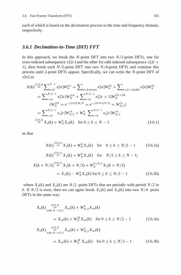
3.6 Fast Fourier Transform (FFT) 165
each of which is based on the decimation process in the time and frequency domain,respectively.
3.6.1 Decimation-in-Time (DIT) FFT
In this approach, we break the N -point DFT into two N/2-point DFTs, one foreven-indexed subsequence x[2r ] and the other for odd-indexed subsequence x[2r +1], then break each N/2-point DFT into two N/4-point DFTs and continue thisprocess until 2-point DFTs appear. Specifically, we can write the N -point DFT ofx[n] as
X (k)(3.4.2)=
∑N−1
n=0x[n]W k n
N =∑
n=2r (even)x[n]W kn
N +∑
n=2r+1(odd)x[n]W kn
N
=∑N/2−1
r=0x[2r ]W 2rk
N +∑N/2−1
r=0x[2r + 1]W (2r+1)k
N
(W 2rkN = e− j2π (2r )k/N = e− j2πrk/(N/2) = W rk
N/2)
=∑N/2−1
r=0xe[r ]W rk
N/2 + W kN
∑N/2−1
r=0xo[r ]W rk
N/2
(3.4.2)= Xe(k) + W kN Xo(k) for 0 ≤ k ≤ N − 1 (3.6.1)
so that
X (k)(3.6.1)= Xe(k) + W k
N Xo(k) for 0 ≤ k ≤ N/2 − 1 (3.6.2a)
X (k)(3.6.1)= Xe(k) + W k
N Xo(k) for N/2 ≤ k ≤ N − 1;
X (k + N/2)(3.6.1)= Xe(k + N/2) + W k+N/2
N Xo(k + N/2)
= Xe(k) − W kN Xo(k) for 0 ≤ k ≤ N/2 − 1 (3.6.2b)
where Xe(k) and Xo(k) are N/2 -point DFTs that are periodic with period N/2 ink. If N/2 is even, then we can again break Xe(k) and Xo(k) into two N/4 -pointDFTs in the same way:
Xe(k)(3.6.1)=
with N→N/2Xee(k) + W k
N/2 Xeo(k)
= Xee(k) + W 2kN Xeo(k) for 0 ≤ k ≤ N/2 − 1 (3.6.3a)
Xo(k)(3.6.1)=
with N→N/2Xoe(k) + W k
N/2 Xoo(k)
= Xoe(k) + W 2kN Xoo(k) for 0 ≤ k ≤ N/2 − 1 (3.6.3b)

166 3 Discrete-Time Fourier Analysis
If N = 2N L OG2, we repeat this procedure N L OG2−1 times to obtain N/2 2 -pointDFTs, say, for N = 23, as
Xee(k) =∑N/4−1
n=0xee[n]W kn
N/4 = x[0] + (−1)k x[4] (3.6.4a)
with xee[n] = xe[2n] = x[22n]
Xeo(k) =∑N/4−1
n=0xeo[n]W kn
N/4 = x[2] + (−1)k x[6] (3.6.4b)
with xeo[n] = xe[2n + 1] = x[22n + 2]
Xoe(k) =∑N/4−1
n=0xoe[n]W kn
N/4 = x[1] + (−1)k x[5] (3.6.4c)
with xoe[n] = xo[2n] = x[22n + 1]
Xoo(k) =∑N/4−1
n=0xoo[n]W kn
N/4 = x[3] + (−1)k x[7] (3.6.4d)
with xoo[n] = xo[2n + 1] = x[22n + 2 + 1]
Along with this procedure, we can draw the signal flow graph for an 8-point DFTcomputation as shown in Fig. 3.15(a). By counting the number of branches witha gain W r
N (representing multiplications) and empty circles (denoting additions),we see that each stage needs N complex multiplications and N complex additions.Since there are log2 N stages, we have a total of N log2 N complex multiplicationsand additions. This is a substantial reduction of computation compared with thedirect DFT computation, which requires N 2 complex multiplication and N (N − 1)complex additions since we must get N values of X (k) for k = 0 : N −1, each X (k)requiring N complex multiplications and N − 1 complex additions.
Remark 3.8 Data Rearrangement in “Bit Reversed” OrderThe signal flow graph in Fig. 3.15 shows that the input data x[n] appear in the
bit reversed order:Position Binary equivalent Bit reversed Sequence index
3 → 011 → 110 → 6
4 → 100 → 001 → 1
Remark 3.9 Simplified Butterfly Computation
(1) The basic computational block in the flow graph (Fig. 3.15(b)), called a butterfly, for stage m + 1 represents the following operations such as Eq. (3.6.2):
Xm+1(p) = Xm(p) + W rN Xm(q), with q = p + 2m (3.6.5a)
Xm+1(q) = Xm(p) + W r+N/2N Xm(q) = Xm(p) − W r
N Xm(q) (3.6.5b)
(∵ W r+N/2N = −W r
N )

3.6 Fast Fourier Transform (FFT) 167
Position0
1
x [0] = xee[0]W2
0 W40
W41
W42
W43
W40
W41
W42
W43
WN0
WN0
WN1
WN2
WN3
WN1
WN2
WN
WN
3
WN4
WN5
WN6
WN7
W20
W20
W20
W21
W21
W21
W21
r
= –WNWNrr + N/2
x [4] = xee[1]
2 x [2] = xeo[0]
3
4
x [6] = xeo[1]
x [1] = xoe[0]
Xeo(0)
Xee(1)
Xee(0)
Xeo(1)
Xoe(0)
Xoe(1)
Xoo(0)
Xoo(1)
Xm(p)
Xm(q)
Xm+1(p)
Xm+1(q)WN
r
Xm(p)
Xm(q)
Xm+1(p)
Xm+1(q)
Xe(2)
Stage 3Stage 2Stage 1
Xe(1)
Xe(0)
Xe(3)
Xo(0)
Xo(1)
Xo(2)
Xo(3)
X(2)
X(1)
X(0)
X(3)
X(4)
X(5)
X(6)
X(7)
5 x [5] = xoe[1]
6
(a) Signal flow graph of DIT(decimation-in-time) FFT algorithm for computing an N = 8-point DFT
(c) Signal flow graph of DIT(decimation-in-time) FFT algorithm (with simplified butterfly pattern) for computing an N = 8-point DFT
(b) Simplifying the butterfly computation
x [3] = xoo[0]
7
⇒
x [7] = xoo[1]
x [0]
W40
W20
W20
W20
W20
W40
W41
W41
–1
–1
–1
–1
–1
–1
–1
–1
–1
–1
–1
–1
–1
x [4]
x [2]
x [6]
x [1]
X(2)
X(1)
X(0)
X(3)
X(4)
X(5)
X(6)
X(7)
x [5]
x [3]
x [7]
Fig. 3.15 Signal flow graph of DIT(decimation-in-time) FFT algorithm
where p and q are the position indices in stage m + 1. Notice that Xm+1(p)and Xm+1(q), the outputs of the butterfly at stage m + 1 are calculated in termsof Xm(p) and Xm(q), the corresponding values from the previous stage andno other inputs. Therefore, if a scratch memory for storing some intermediateresults is available, Xm+1(p) and Xm+1(q) can be calculated and be placed backinto the storage registers for Xm(p) and Xm(q). Thus only N registers for storingone complex array are needed to implement the complete computation. Thiskind of memory-efficient procedure is referred to as an in-place computation.

168 3 Discrete-Time Fourier Analysis
(2) Noting that the horizontal multiplier is just the negative of the diagonal mul-tiplier, the basic butterfly configuration can be further simplified. Specifically,with T = W r
N Xm(q), we have the simplified butterfly computation
Xm+1(p) = Xm(p) + T
Xm+1(q) = Xm(p) − T
which is depicted in Fig.3.15(b). This reduces the number of complex multi-plications for the DFT computation to half of that with the original butterflycomputation (3.6.5a) (Fig. 3.15(c)):
N log2 N → N
2log2 N
3.6.2 Decimation-in-Frequency (DIF) FFT
An alternative algorithm for computing the DFT results from breaking up ordecimating the transform sequence X (k). It begins by breaking up X (k) as follows:
X (k)(3.4.2)=
∑N−1
n=0x[n]W kn
N =∑N/2−1
n=0x[n]W kn
N +∑N−1
n=N/2x[n]W kn
N
=∑N/2−1
n=0x[n]W kn
N + W k N/2N
∑N/2−1
n=0x[n + N/2]W kn
N
=∑N/2−1
n=0(x[n] + (−1)k x[n + N/2])W kn
N (3.6.6)
We separate this into two groups, i.e., one group of the even-indexed elements (withk = 2r ) and the other group of the odd-indexed elements (k = 2r + 1) of X (k);
X (2r ) =∑N/2−1
n=0(x[n] + x[n + N/2])W 2rn
N (3.6.7a)
=∑N/2−1
n=0(x[n] + x[n + N/2])W rn
N/2 for 0 ≤ r ≤ N/2 − 1
X (2r + 1) =∑N/2−1
n=0(x[n] − x[n + N/2])W (2r+1)n
N (3.6.7b)
=∑N/2−1
n=0(x[n] − x[n + N/2])W n
N W rnN/2 for 0 ≤ r ≤ N/2 − 1
These are N/2 -point DFTs of the sequences (x[n]+ x[n + N/2]) and (x[n]− x[n +N/2])W n
N , respectively. If N = 2N L OG2, we can proceed in the same way until itends up with N/2 2-point DFTs. The DIF FFT algorithm with simplified butterflycomputation and with the output data in the bit reversed order is illustrated for a8-point DFT in Fig. 3.16.

3.6 Fast Fourier Transform (FFT) 169
x [0] X (0)
X (4)
X (2)
X (6)
X (1)
X (5)
X (3)
X (7)–1
–1
–1
–1
–1
–1
–1
–1
–1
–1
–1
–1
x [1]
x [2]
x [3]
x [4]WN
x [5]
x [6]
x [7]
0
WN /20
WN /40
WN /40
WN /40
WN /40
WN /20
WN /21
WN /21
WN1
WN2
WN3
Fig. 3.16 Signal flow graph of DIF(decimation-in-frequency) FFT algorithm (with simplifiedbutterfly pattern) for computing an N = 8-point DFT
3.6.3 Computation of IDFT Using FFT Algorithm
The inverse DFT is given by Eq. (3.4.3) as
x[n] = IDFTN {X (k)} = 1
N
∑N−1
k=0X (k)e j2πkn/N
= 1
N
∑N−1
k=0X (k)W −kn
N for n = 0 : N − 1 (3.6.8)
Comparing this with the DFT formula (3.4.2), we see that the computational pro-cedure remains the same except that the twiddle factors are negative powers of WN
and the output is scaled by 1/N . Therefore, an inverse fast Fourier transform (IFFT)program can be obtained from an FFT algorithm by replacing the input data x[n]’swith X (k)’s, changing the exponents of WN to negative values, and scaling the lastoutput data by 1/N .
An alternative way to get the IDFT by using the FFT algorithm is derived bytaking the complex conjugate of the IDFT formula (3.4.3) or (3.6.8) as follows:
x∗[n] = 1
N
∑N−1
k=0X∗(k)W kn
N = 1
NFFT{X∗(k)};
x[n] = 1
N
(FFT{X∗(k)} )∗ (3.6.9)
It is implied that we can get x[n] = IDFTN {X (k)} by taking the complex conjugateof X (k), applying the FFT algorithm for X∗(k), taking the complex conjugate of theoutput, and scaling by 1/N .
The MATLAB built-in functions “fft(x,N)”/“ifft(X,N)” implement theN-point FFT/IFFT algorithm for the data x[n]/X (k) given as their first input argu-ment if the second input argument N is given as a power of 2 or if N is not given and

170 3 Discrete-Time Fourier Analysis
the length of the given data is a power of 2. If the length of the data sequence differsfrom the second input argument N, it will be zero-padded or truncated so that theresulting length will be N.
3.7 Interpretation of DFT Results
In general, the DFT takes a complex-valued sequence {x[n], n = 0 : N − 1} andproduces another complex-valued sequence {X (k), k = 0 : N − 1}. Then, whatis the physical meaning or practical usage of it? To understand it, let us take someexamples where we think of a discrete sequence x[n] as the discrete-time version ofan analog signal x(t) such that x[n] = x(nT ).
Example 3.16 DFT Spectrum of a Single-Tone Sinusoidal Wave [L-1]Suppose we have a continuous-time signal
x(t) = cos (ω1t) = cos
(15
4π t
)with ω1 = 15
4π (E3.16.1)
Let us use the MATLAB function “fft()” to find the DFT spectrum of {x[n] =x(nT ), n = 0 : N−1} with different sampling interval T and DFT size or number ofsample points N . Then we will discuss how we can read the frequency informationabout x(t) from the DFT spectrum, which has different shape depending on thesampling interval T and DFT size N .
(a) Let the sampling interval and number of samples (DFT size) be T = 0.1 andN = 16, respectively so that the discrete-time sequence will be
xa[n] = cos
(15
4π t
)∣∣∣∣t=nT =0.1n
= cos
(3
8πn
), n = 0, 1, · · · , 15
(E3.16.2)
The magnitude spectrum of this sequence, i.e., the magnitude of Xa(k) =DFT16{xa[n]} is depicted in Fig. 3.17(a). It has a spike at the frequency indexk = 3 corresponding to the digital and analog frequencies as
Ω3 = 3Ω0 = 32π
N= 6π
16= 3π
8[rad/sample]
→ ω(1.1.15)= Ω3
T= 3π
8 × 0.1= 15π
4[rad/s] (E3.16.3)
This analog frequency agrees exactly with the real frequency of the originalsignal (E3.16.1). Note that |Xa(k)| has another spike at the frequency indexk = 13, which virtually corresponds to k = 13 − N = −3, but it is just like the

3.7 Interpretation of DFT Results 171
0
1xa[n]
xc [n]
Xa(k )
0
–1
5
1
0
10
00 8 16 24 31
16
–1
0 10 20
Picket Fense Effect Spectral Leakage
30
00 4 8 12 15
5
8
2π
(a) T=0.1, N=16 (b) T=0.05, N=16 (faster and shorter)
(c) T=0.05, N=32 (faster sampling) (d) T=0.1, N=32 (longer interval)
: DFT: DTFT
: DFT: DTFT
: DFT: DTFT
: DFT: DTFT
10 15n
1 xb[n]
0
–1
0 5 10 15n
k
n
xd[n]1
0
–1
0 10 20 30n
k
N
2πN
Xb(k )5
00 4 8 12 15
2π
k
N
Xc(k ) 10
00 8 16 24 31
16
k
Xd(k )
Ω0= Ω0=
Ω0=
Fig. 3.17 DFT spectra of discrete-time sinusoidal sequences having a single tone
mirror image of k = 3. It can be assured by writing the discrete-time sequence(E3.16.2) as
x [n] = 1
2
(e j 3π n/8 + e− j 3π n/8
)IDFT (3.4.3)= 1
N
(N
2e j 2π3 n/N + N
2e− j 2π3 n/N
)∣∣∣∣N=16
(E3.16.4)
= 1
16
(8 e j 2π3 n/16 + 8 e j 2π (13) n/16) = 1
N
∑N−1
k=0X (k) e j 2πk n/N
This explains why the magnitude of the DFT spectrum has two spikes of 8 atk = 3 and N − 3 = 13.
(b) Let the sampling interval and number of samples (DFT size) be T = 0.05(up-sampling) and N = 16, respectively so that the discrete-time sequencewill be
xb[n] = cos
(15
4π t
)∣∣∣∣t=nT =0.05n
= cos
(3
16πn
), n = 0, 1, · · · , 15
(E3.16.5)
The magnitude spectrum of this sequence, i.e., the magnitude of Xb(k) =DFT16{xb[n]} is depicted in Fig. 3.17(b), which looks quite different from

172 3 Discrete-Time Fourier Analysis
Fig. 3.17(a). That is, so many nonzero values show up here and there in themagnitude spectrum, though the highest two values occur at k = 1 and 2. It isbecause the picket fence effect (due to the frequency domain sampling of DFT)hides the spectral peak, allowing the many side lobes (resulting from the spec-tral leakage due to the time domain windowing) to be seen. This is a contrast tothe other cases where the picket fence effect coincidentally hides the side lobesexcept the main peak as if by magic. Still we might fake a “far-fetched” storyabout the frequency corresponding to k = 1.5 (between 1 and 2) as
Ω1.5 = 1.5Ω0 = 1.52π
N= 3π
16[rad/sample]
→ ω(1.1.15)= Ω1.5
T= 3π
16 × 0.05= 15π
4[rad/s] (E3.16.6)
This agrees with the result of (a), showing the right frequency information.(c) Let the sampling interval and DFT size be T = 0.05 (up-sampling) and N = 32
(more sampling), respectively so that the discrete-time sequence will be
xc[n] = cos
(15
4π t
)∣∣∣∣t=nT =0.05n
= cos
(3
16πn
), n = 0, 1, · · · , 31
(E3.16.7)
The magnitude spectrum of this sequence, i.e., the magnitude of Xc(k) =DFT32{xc[n]} is depicted in Fig. 3.17(c). Like Fig. 3.17(a), it has two spikesat k = 3 and N − 3 = 29 with only a difference in their amplitude (16), whichis two times as large as those in (a) because of the increased number of samples(N = 32). Thus we can read the digital and analog frequencies as
Ω3 = 3Ω0 = 32π
N= 6π
32= 3π
16[rad/sample]
→ ω(1.1.15)= Ω3
T= 3π
16 × 0.05= 15π
4[rad/s] (E3.16.8)
This analog frequency also agrees exactly with the real frequency of the originalsignal (E3.16.1).
(d) Let the sampling interval and DFT size be T = 0.1 and N = 32 (longerinterval/more sampling), respectively so that the discrete-time sequence will be
xd [n] = cos
(15
4π t
)∣∣∣∣t=nT =0.1n
= cos
(3
8πn
), n = 0, 1, · · · , 31
(E3.16.9)
The magnitude spectrum of this sequence, i.e., the magnitude of Xd (k) =DFT32{xd [n]} is depicted in Fig. 3.17(d). It has two spikes at k = 6 andN − 6 = 26, which tells us about the existence of the digital and analog

3.7 Interpretation of DFT Results 173
frequencies as
Ω6 = 6Ω0 = 62π
N= 12π
32= 3π
8[rad/sample]
→ ω(1.1.15)= Ω6
T= 3π
8 × 0.1= 15π
4[rad/s] (E3.16.10)
This analog frequency also agrees exactly with the real frequency of the originalsignal (E3.16.1).
Example 3.17 DFT Spectrum of a Multi-Tone Sinusoidal WaveSuppose we have a continuous-time signal
x(t) = sin(ω1t) + 0.5 cos(ω2t) = sin(1.5π t) + 0.5 cos(3π t) (E3.17.1)
with ω1 = 1.5π and ω2 = 3π
Figure 3.18 shows the four different discrete-time versions of this signal and theirDFT spectra, which will be discussed below.
(a) With sampling interval T = 0.1 and DFT size N = 32, the discrete-timesequence will be
xa[n] = x(nT )|T =0.1 = sin(0.15πn) + 0.5 cos(0.3πn), n = 0, 1, · · · , 31
(E3.17.2)
The magnitude spectrum depicted in Fig. 3.18(a) is large at k = 2 & 3 and 4 &5 and they can be alleged to represent two tones, one between kω0 = kΩ0/T =2πk/N T = 2πk/3.2
k=2= 1.25 π and kω0k=3= 1.875 π and the other between
kω0k=4= 2.5 π and kω0
k=5= 3.125 π . Of these two tones, the former correspondsto ω1 = 1.5π (with larger amplitude) and the latter to ω2 = 3π (with smalleramplitude).
(b) With shorter sampling interval T = 0.05 (up-sampling) and larger DFT sizeN = 64, the discrete-time sequence will be
xb[n] = x(nT )|T =0.05 = sin(0.075πn) + 0.5 cos (0.15πn), (E3.17.3)
n = 0, 1, · · · , 63
For all the up-sampling by a factor of 2, the magnitude spectrum depicted inFig. 3.18(b) does not present us with any more information than (a). Why?Because all the frequency components (ω1 = 1.5π and ω2 = 3π ) arealready covered within the principal analog frequency range [−π/T, π/T ]with T = 0.1, there is nothing to gain by expanding it via shorter samplinginterval.

174 3 Discrete-Time Fourier Analysis
1 1
0
0 10 20 30 40 50 60
–1
–2
120
0 5 10 20 30 40 50 60
10
0
1
0
0 10 20 30 40 50 60
–1
–2
30
20
0 5 10 20 30 40 50 60
10
0
15
10
0 105 20 30 40 50 60
5
0
1
0
0 10 20 30 40 50 60
–1
–2
10
0
0 10(a) T=0.1, N=32
(c) T=0.1, N=64 (zero-padding) (d) T=0.1, N=64 (longer interval)
(b) T=0.05, N=64 (faster sampling)
xa[n]
Xa(k )
xb[n]
xc[n]
20 30
5 10 20 30
5
0
0
–1
–2
xd[n]
Xc(k ) Xd(k )
zero-padding
Xb(k )
Fig. 3.18 DFT spectra of a two-tone sinusoidal wave
(c) With the same sampling interval T = 0.1, but with larger DFT size N = 64 (byzero-padding), the discrete-time sequence will be
xc[n] ={
xa[n] for n = 0, 1, · · · , 31
0 for n = 32, · · · , 63(E3.17.4)
The magnitude spectrum depicted in Fig. 3.18(c) is large at k = 4 & 5 and9 & 10 and they can be alleged to represent two tones, one between kω0 =kΩ0/T = 2πk/N T = 2πk/6.4
k=4= 1.25 π and kω0k=5= 1.5625 π and the other
between kω0k=9= 2.8125 π and kω0
k=10= 3.125 π . Comparing this with the resultobtained in (a), we see that larger DFT size by zero-padding can yield betterresolution for the spectrum.
(d) With the same sampling interval T = 0.1, but with larger DFT size N = 64 (bymore sampling), the discrete-time sequence will be
xd [n] = x(nT )|T =0.1 = sin(0.15πn) + 0.5 cos(0.3πn), n = 0, 1, · · · , 63(E3.17.5)

3.7 Interpretation of DFT Results 175
The magnitude spectrum depicted in Fig. 3.18(d) is strikingly large at k = 5and 10, which can be alleged to represent two tones of kω0 = 2πk/N T =2πk/6.4
k=5= 1.5625 π and kω0k=10= 3.125 π . Comparing this with the result
obtained in (a), we see that larger DFT size by more sampling can improvethe spectrum resolution. Comparing this with (c), we see that more samplingcan yield better resolution than zero-padding as it collects more informationabout the signal.
Example 3.18 DFT Spectrum of a Triangular PulseConsider the following sequences that are obtained by sampling the continuous-
time triangular wave x8(t) = 2(λ2(t) − λ2(t − 4)) of period 8 and with peak-to-peak range between −2 and +2. Let us consider the DFT magnitude spectra of thesequences that are depicted in Fig. 3.18.
(a) With sampling interval T = 1 and DFT size N = 8, the discrete-time sequencewill be
xa[n] = x8 (nT )|T =1 , n = 0, 1, · · · , 7 (E3.18.1)
The 8-point DFT magnitude spectrum of xa[n] together with the CTFT mag-nitude spectrum of the single-period triangular pulse x8(t) (Eq. (E3.11.3)) isdepicted in Fig. 3.19(a).
(b) With shorter sampling interval T = 0.5 (up-sampling) and larger DFT sizeN = 16, the discrete-time sequence will be
xb[n] = x8 (nT )|T =0.5 , n = 0, 1, · · · , 15 (E3.18.2)
The 16-point DFT magnitude spectrum of xb[n] together with the CTFT magni-tude spectrum of the single-period triangular pulse x8(t) is depicted inFig. 3.19(b). It shows that the DFT is similar to the CTFT for the expandedprincipal analog frequency range [−π/T, π/T ].
(cf.) Note that to be compared with the DFT, the CTFT spectrum has beenscaled not only vertically in consideration for the sampling interval T(Eq. (3.5.7) or Remark 3.7(2)) and the number of sample points, butalso horizontally in consideration for the relationship between the digitalfrequency Ω and analog frequency ω = Ω/T .
(c) With the same sampling interval T = 1, but with larger DFT size N = 16 (byzero-padding), the discrete-time sequence will be
xc[n] ={
xa[n] for n = 0, 1, · · · , 7
0 for n = 8, · · · , 15(E3.18.3)

176 3 Discrete-Time Fourier Analysis
2
(a) T = 1, N = 8 (b) T = 0.5, N = 16 (c) T = 1, N = 16 (d) T = 1, N = 16
(e) T = 0.5, N = 16 (f) T = 2, N = 4 (g) T = 2, N = 8 (h) T = 1, N = 16
t00
0 2 4 60
5CTFT CTFT
CTFTCTFTDTFT
DFT
2 4 6
–2
k
k
x8(t)
xa [n]
xb [n]
xc [n] xd [n]
Xa (k)
2
t t t t00 2 4 6
–2
2
00 2 4 6
–2
2
00 4 8 12
–2
2
00 4 8 12
–2
2
00 4 8 12t
–2
xe [n]
xf [n]
xg [n] xh [n]
2
t t00 2 4 6
Up-sampling
Spectal leakageBlurred
Down-sampling& Zero-padding
More sampling & Zero - padding
Zero-padding
Zero-insertion
Down-sampling
More sampling
–2
2
00 4 8 12
–2
0 4 8 12
00
5
4 8 12k
00
5
0
5
0
10
1 2 3k
0 2 4 6k
0 4 8 12
0
10
k0 4 8 12
0
5
k0 4 8 12
0
10
k
Xe (k)Xf (k)
Xg(k)
Xh(k)
Xb (k) Xe (k) Xd (k)
∼
Fig. 3.19 DFT spectra of various discrete-time versions of a triangular wave
Figure 3.19(c) shows that the DFT becomes closer to the DTFT spectrum,while it has the same principal analog frequency range for which it is similar tothe CTFT.
(d) With the same sampling interval T = 1, but with larger DFT size N = 16 (bymore sampling), the discrete-time sequence will be
xd [n] ={
xa[n] for n = 0, 1, · · · , 7
xa[n − 8] for n = 8, · · · , 15(E3.18.4)
Figure 3.19(d) shows that we gained nothing with more sampling and largerDFT size in contrast with the case of Example 3.17(d). However, we lostnothing with more sampling.
(e) With larger DFT size N = 16 by zero-insertion, i.e., inserting one zero betweenthe samples, the discrete-time sequence will be
xe[n] ={
xa[n/2] for n = 0, 2, · · · , 14 (even)
0 for n = 1, 3, · · · , 15 (odd)(E3.18.5)
Figure 3.19(e) shows that zero-insertion results in the periodic extension ofthe DFT spectrum. This has an interpretation that zero-insertion increases thevariation rate of the signal, producing the high frequency components.
(f) With longer sampling interval T = 2 (down-sampling or subsampling) andsmaller DFT size N = 4, the discrete-time sequence will be
x f [n] = xa[2n], n = 0, 1, · · · , 3 (E3.18.6)

3.7 Interpretation of DFT Results 177
Figure 3.19(f) shows that down-sampling compresses the principal analogfrequency range and besides, smaller DFT size harms the spectrum resolution.
(g) With longer sampling interval T = 2 (down-sampling or subsampling), butwith the same DFT size N = 8 (by zero-padding), the discrete-time sequencewill be
xg[n] ={
x f [n] for n = 0, 1, · · · , 3
0 for n = 4, 5, · · · , 7(E3.18.7)
Figure 3.19(g) shows that zero-padding may help the spectrum to look better,but it does not recover the spectrum damaged by down-sampling.
(h) With the same sampling interval T = 1, but with larger DFT size N = 16(by more sampling partly and zero-padding partly), the discrete-time sequencewill be
xh[n] ={
xd [n] for n = 0, 1, · · · , 11
0 for n = 12, · · · , 15(E3.18.8)
Figure 3.19(h) shows that zero-padding may help the spectrum to look bettercompared with (d).
Remark 3.10 DFS/DFT (Discrete Fourier Series/Transform) and SpectralLeakage
(1) Generally, the DFT X (k) is complex-valued and denotes the magnitude &phase of the signal component having the digital frequency Ωk = kΩ0 =2πk/N [rad/sample], which corresponds to the analog frequency ωk = kω0 =kΩ0/T = 2πk/N T [rad/s]. We call Ω0 = 2π/N and ω0 = Ω0/T (N :DFT size) the digital/analog fundamental or resolution frequency since it isthe minimum digital/analog frequency difference that can be distinguished bythe N -point DFT. Note that the frequency indices k = 0 and N/2 represent theDC component (Ω = 0) and the virtually highest digital frequency component(ΩN/2 = N/2 × 2π/N = π ), respectively.
(2) As illustrated in Figs. 3.17(b) and 3.18(a)-(d), if a periodic signal does not gothrough a multiple of periods within the sampled signal range [0, N T ), its DFTspectrum is dirty. This is because the spectral leakage is not hidden by thepicket fence effect. It seems that we might avoid this problem by setting thesampled signal range so that it covers exactly a multiple of the period of thesignal. However, it is only our desire because we hardly know in advance thefrequency contents of the signal and besides, most signals have many frequencycomponents.
(3) The spectral leakage problem is always in the midst of DFT because it isinherently due to the time-domain windowing as can be observed in the DTFTspectrum of Fig. 3.5(b3). Then, how could the DFT spectra of Figs. 3.17(a),(c), and (d) be free from the spectral leakage? The fact is that we could not

178 3 Discrete-Time Fourier Analysis
see the existing spectral leakage (as shown by the DTFT spectrum plotted indotted lines) because the picket fence effect [D-1] of DFT (attributed to thefrequency-domain sampling of DTFT) coincidentally happens to hide the manyside lobe ripples except the main peaks.
(4) From another point of view, we might put the responsibility for spectral leakageon the assumption of DFT that every signal is periodic with period equal tothe DFT size, which is hard to be true. As a measure to alleviate the spectralleakage problem, there is a smooth windowing technique [W-1] that can reducethe “faked” abrupt change of the signal (at both ends of the signal range) causedby the rectangular windowing. Interested readers can see Problem 3.14.
Through the examples given above, we have already observed how the DFT spec-trum is affected by the sampling interval, DFT size, zero-padding, and so on. Theobservations are summarized as follows:
Remark 3.11 The Effects of Sampling Period (Interval) T and DFT Size Non DFT
(1) Shorter sampling interval expands the principal analog frequency range[−π/T, π/T ] so that it can help higher frequency components to be reflectedon the DFT spectrum if every frequency component is not covered within thepresent principal analog frequency range.
(2) Larger DFT size (by zero-padding or more sampling) may help the (discrete)DFT spectrum to become closer to the (continuous) DTFT spectrum and thatwith better frequency resolution.
3.8 Effects of Signal Operations on DFT Spectrum
In this section, we summarize the formulas for finding the DFTs of different versionsof a signal from the DFT of the original one. They will be of help in understandingthe effect of self-repetition, zero-padding, zero-insertion, and so on.
Let the DFT of a finite-duration sequence x[n] be
X (k) =∑N−1
n=0x[n]e− j2πkn/N
=∑N−1
n=0x[n]W kn
N with WN = e− j 2π/N for k = 0 : N − 1 (3.8.1)
(a) Flipping: xa[n] = x[N − 1 − n]
Xa(k) =∑N−1
n=0x[N − 1 − n]W kn
Nn→N−1−m=
∑0
m=N−1x[m]W k(N−1−m)
N
m→n=∑N−1
n=0x[n]W −kn
N W −kN = X (N − k)W −k
N (3.8.2)

3.8 Effects of Signal Operations on DFT Spectrum 179
(b) Frequency-shifting: xb[n] = (−1)n x[n]
Xb(k) =∑N−1
n=0(−1)n x [ n] W k n
N
=∑N−1
n=0x[n] W k n
N W (N/2) nN = X (k + N/2) (3.8.3)
(c) Zero-Padding: xc[n] ={
x[n] for n = 0, 1, · · · , N − 1
0 for n = N , · · · , 2N − 1
Xc(k) =∑2N−1
n=0xc[n]W kn
2N =∑N−1
n=0x[n]W (k/2)n
N = X (k/2) (interpolation)(3.8.4)
(d) Self-Repetition: xd [n] ={
x[n] for n = 0, 1, · · · , N − 1
x[n − N ] for n = N , · · · , 2N − 1
Xd (k) =∑2N−1
n=0xd [n]W kn
2N =∑N−1
n=0x[n]W (k/2)n
N +∑2N−1
n=Nx[n − N ]W (k/2)n
N
n→m+N=∑N−1
n=0x[n]W (k/2)n
N +∑N−1
m=0x[m]W (k/2)(m+N )
N
=∑N−1
n=0x[n]W (k/2)n
N +∑N−1
n=0x[n]W (k/2)n
N W (N/2)kN (3.8.5)
= X (k/2) + (−1)k X (k/2) =⎧⎨⎩
2X (k/2) for k even
0 for k odd(zero-insertion)
(e) Zero-Insertion: xe[n] ={
x[n/2] for n even0 for n odd
Xe(k) =∑2N−1
n=0xe[ n] W k n
2N =∑2N−1
n=evenx [ n/2] W kn
2N
n=2m=∑N−1
m=0x[m] W 2km
2Nm→n=
∑N−1
n=0x[n] W k n
N = X (k)
={
X (k) for k = 0, 1, · · · , N − 1X (k − N ) for k = N , · · · , 2N − 1
(self-repetition) (3.8.6)
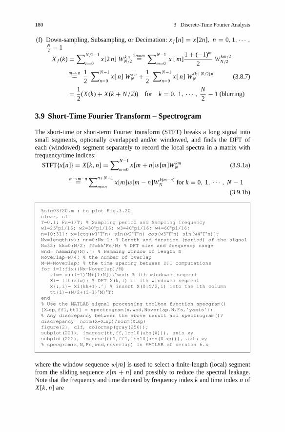
180 3 Discrete-Time Fourier Analysis
(f) Down-sampling, Subsampling, or Decimation: x f [n] = x[2n], n = 0, 1, · · · ,N2 − 1
X f (k) =∑N/2−1
n=0x[2 n] W k n
N/22n=m=
∑N−1
m=0x [ m]
1 + (−1)m
2W km/2
N/2
m→ n= 1
2
∑N−1
n=0x[ n] W k n
N + 1
2
∑N−1
n=0x[ n] W (k+N/2) n
N (3.8.7)
= 1
2(X (k) + X (k + N/2)) for k = 0, 1, · · · ,
N
2− 1 (blurring)
3.9 Short-Time Fourier Transform – Spectrogram
The short-time or short-term Fourier transform (STFT) breaks a long signal intosmall segments, optionally overlapped and/or windowed, and finds the DFT ofeach (windowed) segment separately to record the local spectra in a matrix withfrequency/time indices:
STFT{x[n]} = X [k, n] =∑N−1
m=0x[m + n]w[m]W km
N (3.9.1a)
m→m−n=∑n+N−1
m=nx[m]w[m − n]W k(m−n)
N for k = 0, 1, · · · , N − 1
(3.9.1b)
%sig03f20.m : to plot Fig.3.20clear, clfT=0.1; Fs=1/T; % Sampling period and Sampling frequencyw1=25∗pi/16; w2=30∗pi/16; w3=40∗pi/16; w4=60∗pi/16;n=[0:31]; x=[cos(w1∗T∗n) sin(w2∗T∗n) cos(w3∗T∗n) sin(w4∗T∗n)];Nx=length(x); nn=0:Nx-1; % Length and duration (period) of the signalN=32; kk=0:N/2; ff=kk∗Fs/N; % DFT size and frequency rangewnd= hamming(N).’; % Hamming window of length NNoverlap=N/4; % the number of overlapM=N-Noverlap; % the time spacing between DFT computationsfor i=1:fix((Nx-Noverlap)/M)
xiw= x((i-1)∗M+[1:N]).∗wnd; % ith windowed segmentXi= fft(xiw); % DFT X(k,i) of ith windowed segmentX(:,i)= Xi(kk+1).’; % insert X(0:N/2,i) into the ith columntt(i)=(N/2+(i-1)∗M)∗T;
end% Use the MATLAB signal processing toolbox function specgram()[X sp,ff1,tt1] = spectrogram(x,wnd,Noverlap,N,Fs,’yaxis’);% Any discrepancy between the above result and spectrogram()?discrepancy= norm(X-X sp)/norm(X sp)figure(2), clf, colormap(gray(256));subplot(221), imagesc(tt,ff,log10(abs(X))), axis xysubplot(222), imagesc(tt1,ff1,log10(abs(X sp))), axis xy% specgram(x,N,Fs,wnd,noverlap) in MATLAB of version 6.x
where the window sequence w[m] is used to select a finite-length (local) segmentfrom the sliding sequence x[m + n] and possibly to reduce the spectral leakage.Note that the frequency and time denoted by frequency index k and time index n ofX [k, n] are
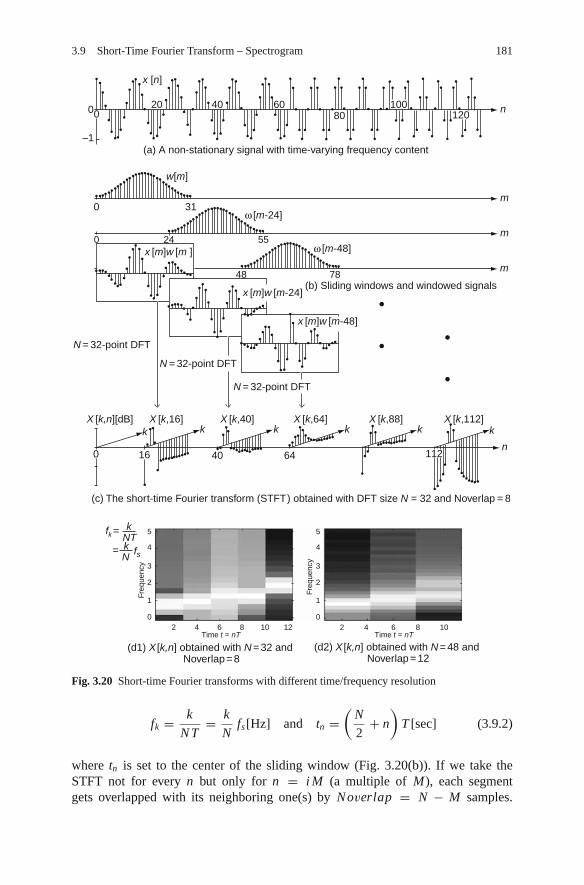
3.9 Short-Time Fourier Transform – Spectrogram 181
200
0 31
0 24 55
48 78
0 16 40 64 112
(a) A non-stationary signal with time-varying frequency content
(b) Sliding windows and windowed signals
(c) The short-time Fourier transform (STFT ) obtained with DFT size N = 32 and Noverlap = 8
(d1) X [k,n] obtained with N = 32 and Noverlap = 8
(d2) X [k,n] obtained with N = 48 and Noverlap = 12
Time t = nT
Freq
uenc
y
Freq
uenc
y
Time t = nT
N = 32-point DFT
N = 32-point DFT
N = 32-point DFT
n
m
m
m
kNT
n
kkkkkk
x [n]
0
–1
40 60 10012080
X [k,n][dB] X [k,16] X [k,40] X [k,64]
fk =
X [k,88] X [k,112]
x [m]w [m-24]
x [m]w [m ]
ω [m-24]
w[m]
ω [m-48]
x [m]w [m-48]
02 4 6 8 10 12 2 4 6 8 10
1
2
3
4
5
0
1
2
3
4
5
k fsN=
0
1
2
3
4
5
Freq
uenc
y
Fig. 3.20 Short-time Fourier transforms with different time/frequency resolution
fk = k
N T= k
Nfs[Hz] and tn =
(N
2+ n
)T [sec] (3.9.2)
where tn is set to the center of the sliding window (Fig. 3.20(b)). If we take theSTFT not for every n but only for n = i M (a multiple of M), each segmentgets overlapped with its neighboring one(s) by Noverlap = N − M samples.

182 3 Discrete-Time Fourier Analysis
Note that M determines the width of interval time between the DFT computations.The MATLAB function “spectrogram()” can be used to find the STFT (seeAppendix E.8).
We run the above MATLAB program “sig03f20.m” to get the STFT X [k, n]of x[n] (Fig. 3.20(a)) as depicted in Fig. 3.20(d1) (with DFT size N = 32 andNoverlap = 8) and (d2) (with N = 48 and Noverlap = 12), which show that thefrequency becomes higher as time goes by. Such a STFT can be used to determineand display the spectrum of a non-stationary signal (such as speech or music) whosefrequency content changes with time.
Now, comparing Fig. 3.20(d1) and (d2), let us consider the effect of segment orwindow duration NT on the time and frequency resolutions of the STFT. We mightsay that the time resolution is NT [sec] (the segment duration) and the frequencyresolution is 1/N T [Hz]. This implies that if we increase or decrease the segmentduration, the time/frequency resolution gets poorer/better or better/poorer, show-ing the trade-off between the time and frequency resolutions. It is an illustrationof uncertainty principle (Remark 2.9(1)) that both time resolution and frequencyresolution cannot be improved. Although the boundary of the uncertainty principle(best simultaneous resolution of both) is reached with a Gaussian window function,the wavelet transform or multi-resolution analysis was devised, which can give agood time/frequency resolution for high/low-frequency components.
3.10 Summary
In this chapter we have defined the discrete-time Fourier transform (DTFT) and thediscrete Fourier series(DFS)/transform(DFT) for discrete-time signals and exam-ined their properties together with their relationship. The DFT of a discrete-timesequence x[n] has been shown to correspond to one period of the discrete-timeFourier series for the periodic extension of x[n]. We have also discussed the FFTalgorithms that deserve the overwhelming popularity owing to their computationalefficiency. This chapter also introduced some examples, which give you some inter-pretation of the DFT and will hopefully help you to gain an insight into physicalmeaning or practical usage of the DFT. It ended up with the introduction of the short-time Fourier transform (STFT), which can easily be obtained by using a MATLABfunction “specgram()” in 6.x versions and “spectrogram()” in 7.x versions.
Problems
3.1 Properties of DTFT (Discrete-Time Fourier Transform)
(a) Prove the frequency-shifting property (3.2.7) by using the DTFT formula(3.1.1) or IDTFT formula (3.1.3).
x[n]e jΩ1n F↔ X (Ω − Ω1) (P3.1.1)

Problems 183
(b) Prove the convolution property (3.2.8).
y[n] = x[n]∗g[n]F↔ Y (Ω) = X (Ω)G(Ω) (P3.1.2)
(c) Prove the modulation property (3.2.9).
y[n] = x[n] m[n]F↔ Y (Ω) = 1
2πX (Ω)∗M(Ω) (P3.1.3)
(d) Prove the summation property (3.2.11) by using the convolution property(3.2.8) together with Eq. (E3.8.6).
∑n
m=−∞ x[m] = x[n] ∗ us[n]F↔
1
1 − e− j ΩX (Ω) + π X (0)
∑∞i=−∞ δ(Ω − 2π i)
(P3.1.4)
3.2 Discrete-Time Hilbert Transformer
(a) Prove that the impulse response of a system, called the Hilbert trans-former, with frequency response
H (Ω) ={− j for 0 < Ω < π
+ j for − π < Ω < 0(P3.2.1)
is
h [n] ={
2/nπ for n : odd0 for n : even
(P3.2.2)
%sig03p 02.mEPS=1e-10; Nx=200; nx=[-Nx:Nx]; W1=0.1∗pi; xn= cos(W1∗nx);Nh=50; nh=[-Nh:Nh]; hn= (mod(nh,2)==1).∗(2/pi./(nh+EPS));yn= conv(hn,xn); ny=Nh+Nx+1+nx; yn1= yn(ny);W=[-50:-1 1:50]∗(pi/50);X= DTFT(xn,W); Xmag= abs(X); Xphase= angle(X);Xphase= (abs(imag(X))>=EPS).∗Xphase;H= DTFT(hn,W); Hmag= abs(H); Hphase= angle(H);Y= DTFT(yn,W); Ymag= abs(Y); Yphase= angle(Y);subplot(331), plot(nx,xn), axis([nx([1 end]) -1.5 1.5])subplot(332), plot(W,Xmag), subplot(333), plot(W,Xphase)subplot(334), plot(nh,hn), axis([nh([1 end]) -1 1])subplot(335), plot(W,Hmag), subplot(336), plot(W,Hphase)subplot(337), plot(nx,yn1, nx,sin(W1∗nx),’r’)subplot(338), plot(W,Ymag), subplot(339), plot(W,Yphase)

184 3 Discrete-Time Fourier Analysis
(b) By taking the IDTFT of Y (Ω) = H (Ω)X (Ω), prove that the output of theHilbert transformer to a sinusoidal input x[n] = cos(Ω0n) is
y[n] = sin( Ω0n) (P3.2.3)
(c) We can run the above program “sig03p 02.m” to rest assured of thefact that the output of the Hilbert transformer to x[n] = cos(0.1πn) isy[n] = sin(0.1πn) where y[n] = h[n]∗x[n] has been obtained from thetime-domain input-output relationship. Identify the statements yieldingthe impulse response h[n], output y[n], and frequency response H (Ω).
3.3 Discrete-Time Differentiator
(a) Prove that the impulse response of a discrete-time differentiator withfrequency response
H (Ω) = jΩ (P3.3.1)
is
h [n] = (−1)n
n(P3.3.2)
(b) By taking the IDTFT of Y (Ω) = H (Ω)X (Ω), prove that the output of thedifferentiator to a sinusoidal input x[n] = sin(Ω0n) is
y[n] = Ω0 cos( Ω0n) (P3.3.3)
(c) By reference to the program “sig03p 02.m”, compose a program and runit to rest assured of the fact that the output of the differentiator to x[n] =sin(0.1πn) is y[n] = 0.1π cos(0.1πn) where y[n] = h[n] ∗ x[n] has beenobtained from the time-domain input-output relationship.
3.4 BPF Realization via Modulation-LPF-Demodulation – Frequency ShiftingProperty of DTFTConsider the realization of BPF of Fig. P3.4(a), which consists of a modulator(multiplier), an LPF, and a demodulator (multiplier). Assuming that the spec-trum of x[n] is as depicted in Fig. P3.4(b), sketch the spectra of the signalss[n], v[n], and y[n].
3.5 Quadrature Multiplexing – Modulation (Complex Convolution) Propertyof DTFTConsider the quadrature multiplexing system depicted in Fig. P3.5 where thetwo signals are assumed to be bandlimited, i.e.,
X1(Ω) = X2(Ω) = 0 for Ω > ΩM (P3.5.1)

Problems 185
–2π –π –π/2
–π/4 π/4
0
2
(b) The spectrum of the input signal x [n ]
(a) A BPF realization via modulation–LPF–demodulation
multiplier multiplier
LPF
x [n] y [n]
G (Ω)
X (Ω)
Ω
s [n] v [n]
ejπn /2 e–jπn /2
π/2 π 2πΩ
1
0
Fig. P3.4
cos Ωcn
–ΩM ΩM
–ΩM ΩM
sin Ωc n
x1[n]
y2[n]
y1[n]v1[n]
v2[n]
s [n] r [n]
x2[n]
multiplier
multiplierLPF
LPF
2
2
Communicationchannel
adder
multiplier
multiplier
adder
Fig. P3.5 Quadrature multiplexing
Assuming that the channel is ideal so that r [n] = s[n], express the spectraS(Ω), V1(Ω), V2(Ω), Y1(Ω), and Y2(Ω) of s[n], v1[n], v2[n], y1[n], andy2[n] in terms of X1(Ω) and X2(Ω).
3.6 Windowing (Complex Convolution) Property of DTFTReferring to Example 3.10, answer the following questions:
(a) In the program “sig03e10.m”, increase the (rectangular) window sizeparameter M and run the program to see the window spectrum and the fre-quency response of the designed FIR filter. Based on the results, describethe shape of the filter frequency response when M is set to infinity.
(b) With the window size parameter M set to 3 as it was, change the shapeof the window into, say, one of the following: Bartlett (triangular), Ham-ming, Hanning, Blackman, and Kaiser. Note that the window sequencescan be generated (as column vectors) by the MATLAB commands,bartlett(), hamming(), hanning(), blackman(), andkaiser(), respectively. Has the ripple of the frequency response beenreduced?

186 3 Discrete-Time Fourier Analysis
3.7 DTFT and CTFT of a Finite-Duration Signal
%sig03p 07.m% Fig. 3.7(To tell the relationship between CTFT and DTFT)EPS=1e-10; T=1; t =[-10:T:10];N=400; f=[-500:500]/N + EPS; % Normalized frequency rangeW=2∗pi∗f; w=W/T; % Digital/Analog frequency rangexn= [zeros(1,7) 1 2 1 0 -1 -2 -1 zeros(1,7)];Xw= inline(’j∗8∗sin(2∗w).∗sinc(w/pi).ˆ2’,’w’);X CTFT= Xw(w); X CTFT mag= abs(X CTFT);Sum of X CTFTs= (Xw(w+2∗pi/T)+Xw(w)+Xw(w-2∗pi/T))/T;X DTFT=DTFT(xn,W); X DTFT mag= abs(X DTFT); X DTFT ph= angle(X DTFT);Discrepancy between CTFT DTFT= norm(X DTFT-Sum of X CTFTs)/norm(X DTFT)subplot(321), stem(t,xn,’.’), hold on, plot(t,xn,’:’)subplot(323), plot(W,X DTFT mag,’b’, W,X CTFT mag/T,’k:’)hold on, plot(W,abs(Sum of X CTFTs),’r:’)
The objective of the above program “sig03p 07.m” is to plot the CTFT spec-trum X1(ω)/T of the unsampled dual triangular pulse signal x1(t) given byEq. (E3.11.3) and the DTFT spectrum X1(Ω) of the triangular pulse sequencex1[n] = x1(nT ) with T = 1. Also, it plots the sum of three CTFTs shiftedby −2π/T , 0, and +2π/T along the analog frequency ω = Ω/T and scaledby 1/T to check the validity of the relationship between the CTFT and DTFTdescribed by Eq. (3.5.7). Modify the program so that it does the same jobwith sampling interval T = 0.5. What can we get by shortening the samplinginterval? Refer to Remark 3.7(2).
3.8 DFT/DFS, DTFT, and CTFS of a Noncausal SignalConsider the dual triangular pulse sequence which would be obtained bysampling x1(t) in Fig. 3.7(a1) with sampling interval T = 0.5.
(a) Use the MATLAB function “fft()” to get the N = 16-point DFTX N (k) of the sequence and plot its magnitude together with the DTFTmagnitude against Ωk = [0 : N − 1] × (2π/N ) and Ω = [−500 :500] × (2π/400), respectively. Note that the DTFT might have beenobtained in Problem 3.7.
(b) Noting that the CTFS coefficients Xk are the samples of the CTFT X (ω)(Eq. (E3.11.3)) at ω = kω0 = 2πk/P = 2πk/N T as described byEq. (2.2.4) or stated in Remark 2.7(2), find the relative errors betweenthe DFT X N (k) and two partial sums of the shifted CTFSs and comparethem to argue for the relationship (3.5.3) between the DFT and CTFS.
E1 = ||X N (k) − Xk/T ||||X N (k)|| and
E2 = ||X N (k) − (Xk+N + Xk + Xk−N )/T ||||X N (k)|| (P3.8.1)

Problems 187
<Hint> You might need to combine some part of the program “sig03p07.m” with the following statements:
xn causal= [0 -0.5 -1 -1.5 -2 -1.5 -1 -0.5 0 0.5 1 1.5 2 1.5 1 0.5];X DFT= fft(xn causal); X DFT mag= abs(X DFT);N=length(xn causal); k=[0:N-1];f0=1/N; fk=k∗f0; W0=2∗pi∗f0; Wk=k∗W0; w0=W0/T;stem(Wk,X DFT mag,’m.’)% (b): Partial sum of CTFSs by Eq.(3.5.3)Sum of Xks= (Xw((k+N)∗w0)+Xw(k∗w0)+Xw((k-N)∗w0))/T;Discrepancy between CTFS and DFT= norm(X DFT-Xw(k∗w0)/T)/norm(X DFT)Discrepancy between CTFS and DFT3= norm(X DFT-Sum of Xks)/norm(X DFT)
3.9 CTFS, CTFT, and DFT/DFS of a Noncausal Sequence
–3 –2
x (t ) (a triangular pulse)
x (t )
x2(t ) (periodic extension with period 2)~
x2(t )~
x∗(t )~
x2[n ] (discrete-time version)~
–0.5–1
1
0 0.5 1 2 3t
T
Fig. P3.9
Consider the triangular pulse signal x(t) of Fig. P3.9, its periodic extensionx2(t) with period P = 2, and its sampled periodic version x∗(t) = x2(t)δT (t)with sampling interval T = 0.5.
(a) Find the CTFT X (ω) of x(t). You can use Eq. (E2.3.4).(b) Find the CTFS Xk of x2(t). You can use the result of (a) and Eq. (2.2.4)
stating that the CTFS coefficients are the samples of the CTFT at ω =kω0 = 2πk/P .
(c) Show that the N = 4-point DFT of the discrete-time version x[n] is
X (k) = [2 1 0 1] (P3.9.1)
(d) Show the validity of the relationship between the CTFS and DFT describedby Eq. (3.5.3) for this case, i.e.,
X (k)(P3.9.1)= [2 1 0 1]
?= 1
T
∑∞m=−∞ Xk+m N (P3.9.2)

188 3 Discrete-Time Fourier Analysis
<Hint> You might need the following formula
∑∞m=0
1
(2m + 1)2= π2
8(P3.9.3)
which can be derived by substituting A = 1, D/P = 1/2 intoEq. (E2.1.6) as
AλD/P (t)(E2.1.6)= 1
P
∑∞k=−∞ ADsinc2
(k
D
P
)A=1, P=2D→
1 = 1
2
∑∞k=−∞ sinc2
(k
2
)
= 1
2
⎛⎝for k=0
1 + for k=even(�=0)0 +
for k=odd∑∞k=2m+1
1
(kπ/2)2
⎞⎠ ;
1
2= 1
2
∑∞m=−∞
1
(2m + 1)2π2/22= 2
∑∞m=−∞
1
(2m + 1)2π2
= 4∑∞
m=0
1
(2m + 1)2π2
3.10 DTFT and DFT of Discrete-Time Periodic SequencesWhen we need to find the DTFT of a periodic sequence xN [n] with period N ,we first get its DFS representation
xN [n](3.4.3)=IDFT
1
N
∑N−1
k=0X N (k)e j2πkn/N (P3.10.1)
with X N (k)(3.4.2)=DFT
∑N−1
n=0xN [n]e− j2πkn/N
and then use Eq. (3.1.5) to obtain the DTFT of xN [n] as
xN [n] = 1
N
∑N−1
k=0X N (k)e j2πkn/N F↔
X (Ω)(P3.10.1)=
(3.1.5)
2π
N
∑∞k=−∞ X N (k)δ
(Ω − 2πk
N
)(P3.10.2)
(a) Verify the validity of this DTFT pair by showing that the IDTFT of(P3.10.2) is xN [n].
F−1{X (Ω)} (3.1.3)= 1
2π
∫2π
X (Ω) e j Ω n dΩ
(P3.10.2)=(1.1.25)
1
N
∑N−1
k=0X N (k) e j 2πkn/N (P3.10.1)= xN [n] (P3.10.3)

Problems 189
(b) Use the DTFT relation (P3.10.2) to show that the DTFT of the discrete-time impulse train
δN [n] =∑∞
m=−∞ δ[n−m N ] (also called the comb sequence) (P3.10.4)
is
DN (Ω) = 2π
N
∑∞k=−∞ δ
(Ω − 2πk
N
)= 2π
N
∑∞k=−∞ δ
(Ω + 2πk
N
)
(P3.10.5)
3.11 Effect of Discrete-Time Sampling on DTFTAs a continuous-time sampling with sampling interval T can be described by
x∗(t)(E2.13.1)= x(t)δT (t) (δT (t) =
∑∞m=−∞ δ(t − mT ) : the impulse train)
so can a discrete-time sampling with sampling interval N be described by
x∗[n] = x[n]δN [n] (δN [n] =∑∞
m=−∞ δ[n − m N ] : the impulse train)
(P3.11.1)
(a) Use the DTFT modulation property (3.2.9) or B.4(9) and Eq. (P3.10.5) toshow that the DTFT of this sampled sequence x∗[n] can be expressed interms of that of the original sequence x[n] as
X∗(Ω) = 1
N
∑∞m=−∞ X
(Ω + 2πm
N
)
= 1
N
∑∞m=−∞ X (Ω + mΩs) with Ωs = 2π
N(P3.11.2)
(b) Show that the DTFT of a decimated sequence xd [n] obtained by removingthe zeros from the sampled sequence x∗[n] = x[n]δN [n] is
Xd (Ω) = X∗
(Ω
N
)(P3.11.3)
(cf.) This conforms with Eq. (3.2.14), which is the scaling property of DTFT.
(c) Substitute Eq. (P3.11.2) into Eq. (P3.11.3) to show that
Xd (Ω) = 1
N
∑N−1
m=0X
(Ω
N+ 2πm
N
)(P3.11.4)

190 3 Discrete-Time Fourier Analysis
1.0
0.0
2.0
0.0
2.0
0.0
2.0
4.0
0.0
2.0
0.0
2.0
0.0
–8.0 –6.0 –4.0 –2.0
(a1) x0(t )
(a2) xa(t )
(a3) x [n ] sampling xa(t ) with T = 0.5
x [n ]
x0(t )x0(t ) )(= sinc
2
0.0 2.0 4.0 6.0 8.0 –3π –2π –π(b1) X0(ω )
X0(ω )
Xa (ω )
X (Ω )
0.0 π 2π 3π
–3π –2π –π 0.0 π 2π 3π
–3π –2π –π(b2) Xa(ω )
(b3) X(Ω ): (P3.11.5) with T = 0.5 from Xa(ω )
–3π –2π –π 0.0 π 2π 3π(b4) X1(Ω ): (P3.11.2) with N = 2 from X (Ω )
–3π –2π –π 0.0 π 2π 3π(b5) Xd (Ω ): (P3.11.3) with N = 2 from X1(Ω )
2.0
0.0
1.0
0.0
1.0
0.0
–3π –2π –π 0.0 π 2π 3π(b6) X3(Ω ): (P3.11.2) with N = 2 from Xd (Ω )
–3π –2π –π 0.0 π 2π 3π(b7) X4(Ω ): (P3.11.2) with N = 2 from X (Ω )
–3πΩ
Ω
Ω
Ω
Ω
Ω
ω
ω
–2π –π 0.0 π 2π 3π(b8) X5(Ω ): (P3.11.5) with T = 2 from Xa(ω )
0.0 π 2π 3π
1.0
0.0–8.0 –6.0 –4.0 –2.0 0.0 2.0 4.0 6.0 8.0
1.0
0.0
1.0
0.0
1.0
0.0
–12 –8 –4 0 4 8 12
(a4) x1[n ] sampling x [n ] with N =2
–12 –8 –4 0 4 8 12
(a5) xd [n ] decimating x1[n ] with N = 2
–6 –4 –2 0 2 4 6
–4 –3 –2 –1 0 1 2 3 4
1.0
0.0
1.0
0.0
1.0
0.0
–12 –8 –4 0 4 8 12
(a6) x3[n ] sampling xd [n ] with N = 2
(a7) x4[n ] sampling x [n ] with N = 4
(a8) x5[n ] ampling xa(t ) with T = 2
–6 –4 –2 0 2 4 6
t
t
t
n
n
n
n
n
n
(t ) )(= sinc2txa(t ) = x0
2 2
Fig. P3.11 Effect of sampling on the spectrum
(d) Let x[n] be obtained from the samples of xa(t) with sampling interval T .Then, from Eq. (3.5.7), we can write
X (Ω) = X∗(ω)|ω=Ω/T(3.5.7)= 1
T
∑∞k=−∞ Xa
(Ω
T+ k
2π
T
)(P3.11.5)

Problems 191
Substitute this into Eq. (P3.11.4) to show that
Xd (Ω) = 1
N T
∑ ∞k=−∞ Xa
(Ω
N T+ 2πk
N T
)(P3.11.6)
(e) Verify the CTFT relation between the signal and its spectrum depicted inFigs. P3.11(a2) and (b2):
xa(t) = x20 (t) = sinc2
(t
2
)F↔ 1
2π2rπ (ω) ∗ 2rπ (ω) (triangular pulse)
(P3.11.7)
Also verify the DTFT relation between the signal and its spectrum depictedin Fig. P3.11(a3) and (b3):
x[n] = x20 [n] = sinc2
(n
4
) F↔ 1
2π4rπ/2(Ω) ∗ 4rπ/2(Ω) (triangular pulse)
(P3.11.8)
(f) Show that the DTFT spectrum X (Ω) of x[n] (Fig. P3.11(a3)) can beexpressed in terms of the CTFT spectrum Xa(ω) of xa(t) (Fig. P3.11(a2)) as
X (Ω) = 2∑∞
k=−∞ Xa(2(Ω − 2πk)) (P3.11.9)
Show that the DTFT spectrum X1(Ω) of x1[n] (Fig. P3.11(a4)) can beexpressed in terms of the DTFT spectrum X (Ω) of x[n] (Fig. P3.11(a3)) as
X1(Ω) = 1
2(X (Ω) + X (Ω + π )) (P3.11.10)
Show that the DTFT spectrum Xd (Ω) of xd [n] (Fig. P3.11(a5)) can beexpressed in terms of the DTFT spectrum X (Ω) of x[n] (Fig. P3.11(a3)) as
Xd (Ω) = 1
2
(X
(Ω
2
)+ X
(Ω + 2π
2
))(P3.11.11)
Show that the DTFT spectrum X3(Ω) of x3[n] (Fig. P3.11(a6)) can beexpressed in terms of the DTFT spectrum Xd (Ω) of x[n] (Fig. P3.11(a5)) as
X3(Ω) = 1
2(Xd (Ω) + Xd (Ω + π )) (P3.11.12)

192 3 Discrete-Time Fourier Analysis
Show that the DTFT spectrum X4(Ω) of x4[n] (Fig. P3.11(a7)) can beexpressed in terms of the DTFT spectrum Xd (Ω) of xd [n](Fig. P3.11(a5)) as
X4(Ω) = 1
4
(Xd (Ω) + Xd
(Ω + π
2
)+ Xd (Ω + π ) + Xd
(Ω + 3
2π
))(P3.11.13)
Show that the DTFT spectrum X5(Ω) of x5[n] (Fig. P3.11(a8)) can beexpressed in terms of the CTFT spectrum Xa(ω) of xa(t) (Fig. P3.11(a2)) as
X5(Ω) = 1
2
∑∞m=−∞ Xa
(Ω + 2mπ
2
)(P3.11.14)
(cf.) The sampled sequences x3[n], x4[n], and x5[n] are all identical tothe impulse sequence and their flat spectra illustrate the extremecase of a spectrum blurred by downsampling.
3.12 Linear Convolution and Correlation Using DFTConsider the following two sequences:
x[n] = [1 2 3 4 5 6 7 8] and y[n] = [1 −2 3] (P3.12.1)
(a) Referring to Remark 1.5, determine the length of the linear convolutionor correlation of the two sequences. Also use the MATLAB command“nextpow2()” to find the smallest power of 2 that is greater than orequal to the expected length of the linear convolution or correlation. Whatis the minimum size N of DFT that can make the FFT operation mostefficient for computing the linear convolution or correlation?
(b) Referring to Sect. 3.4.2, use the N -point FFT to compute the linear con-volution of x[n] and y[n]. Check if the result conforms with that obtainedby using “conv(x,y)”.
(c) It seems that we can use the N -point FFT to compute the correlation ofx[n] and y[n] based on the following facts:
◦ φxy[n](1.4.12b)= x[n] ∗ y[−n]
periodicity of y[n]=with period N
x[n] ∗ y[N − n] (P3.12.2)
◦ x[−n]F↔
(3.2.3)X (−Ω) implies that DFTN {y[N − n]} = Y (N − k)
(P3.12.3)
Noting that y[N − n] can be programmed as “[y(1) fliplr(y(2:end))]”, compose a program to compute the correlation and run it toget φxy[n]. Check if the result conforms with that obtained by using“xcorr(x,y)”.

Problems 193
3.13 DFT Spectra of Sampled Signals
(b)
(d)
20
30
10
00 8 16 32 48 63
k
(c)
30
20
10
00 8 16 32 48 63
k
Xb(k )
20
10
00 8 16 32 48 63 k
(a)
20
10
00 8 16 32 48 63
k
Xd(k )Xc(k )
Xa(k )
Fig. P3.13 DFT spectra of several discrete-time signals
With the sampling period T = 0.1 [s], we have sampled the following signals
(1) 0.5 cos 3π t + sin 2π t(2) cos 3π t + 0.5 sin 2π t(3) 0.5 cos 4π t + sin π t(4) cos 4π t + 0.5 sin π t(5) 0.5 cos 23π t + 0.5 sin 2π t − 0.5 sin 18π t(6) 0.5 sin 21π t + 0.5 cos 24π t + 0.5 cos 16π t
and obtained their DFT spectra as depicted in Fig. P3.13.
(a) Find the corresponding spectrum for each signal from the DFT spectradepicted in Fig. P3.13.
(b) If these signals have been through an anti-aliasing prefilter, which one isexpected to have the DFT magnitude spectrum like |Xa(k)|?
3.14 Spectral Leakage and Windowing TechniqueLet us think about the cause of spectral leakage illustrated in Fig. 3.17(b)and some measure against it. As discussed in Remark 3.10(2), the spectralleakage stems from that any sequence is supposed to have periodicity withperiod N (equal to the DFT size), regardless of its peridocity, just because it isan object sequence of an N -point DFT. More specifically, the sequence xb[n]is supposed to be periodic with period N = 16 as depicted in Fig. P3.14(a),which shows such abrupt changes as discontinuities at both ends. A measure toreduce this abrupt change is to multiply a window sequence whose magnitudedecreases gradually at both ends rather than cuts off abrubtly as the rectangularwindow does. Figure P3.14(b), (c), (d1), and (d2) show a triangular (Bartlett)window wT [n] of length N = 16, the windowed sequence xb[n]wT [n], andthe DFT spectra of xb[n] and xb[n]wT [n]. Comparing the DFT spectra ofunwindowed and windowed sequences, we can see that the windowing has

194 3 Discrete-Time Fourier Analysis
0
0
x b[n ]~
~
x b[n ] wT
[n ]~
~x b[n ] x b[n ]
wT
[n ]
0
0
0
(a) A sequence x b[n ] with its periodicity assumed due to the 16-point DFT
(b) A triangular (Bartlett) window of length N = 16
(c) The windowed sequence and its periodic extension with period N = 16
(d1) The DTF spectrum of unwindowed sequence
DFT { x b[n ] }
(d2) The DTF spectrum of windowed sequence
7
7
8
8
7 8
15
15
15
n
n
n
1
1
–1
0
6
Xb(k) =
~DFT { x b[n ]w [n ] }
4
2
00–8 8–4 4 0
0–8 8–4
2
4
4
1
–1
k k
Fig. P3.14 The effect of windowing on the DFT spectrum
the effect of reducing the spectral leakage. You can try with another windowsuch as the Hamming window or Hanning (raised-cosine) window.
3.15 Spectrum Blurring due to Down/Sub-sampling (Slower Sampling)As can be seen in Fig. 3.19(f) or Eq. (3.8.7), slower sampling (sub-sampling)may make the spectrum blurred.
(a) Noting that x f [n] in Fig. 3.19(f) has been obtained from downsamplingxa[n] by a factor of 2, sketch the DFT spectrum of the sequence whichwill be obtained from downsampling x f [n] by a factor of 2.
(b) Referring to Eq. (3.8.7), determine the condition on which the DFTspectrum is not blurred by downsampling it by a factor of 2.
3.16 Parallel Computation of DFTs for Two Real-valued Sequences (Problem 4.10of [K-2])We can compute the DFTs of two real-valued sequences x1[n] and x2[n] fromthe DFT Y (k) of a complex-valued sequence
y[n] = x1 [n] + j x2 [n] (P3.16.1)

Problems 195
where the DFT of each sequence can be written as
X1(k) = X1R(k) + j X1I (k) =∑N−1
n=0x1[n] cos
(2πkn
N
)
− j∑N−1
n=0x1[n] sin
(2πkn
N
)(P3.16.2a)
X2(k) = X2R(k) + j X2I (k) =∑N−1
n=0x2[n] cos
(2πkn
N
)
− j∑N−1
n=0x2[n] sin
(2πkn
N
)(P3.16.2b)
(a) Show that, since xi [n], i = 1 & 2, is real, Xi R(k) = Re{Xi (k)} is evenand Xi I (k) = Im{Xi (k)} is odd via the conjugate symmetry (3.2.5) orTable B.5(4) so that
Xi R(k) = Xi R(−k)rN [k] = Xi R(N − k)
= Xi R(N − k) for k = 1, · · · , N − 1 (P3.16.3a)
Xi I (k) = −Xi I (−k)rN [k] = −Xi I (N − k)
= −Xi I (N − k) for k = 1, · · · , N − 1 (P3.16.3b)
where rN [k] = us[k] − us[N − k] is a rectangular pulse sequence.(b) Show that the real and imaginary parts of Y (k) = DFTN {y[n]} can be
expressed in terms of X1R(k), X1I (k), X2R(k), and X2I (k) as
Y (k) = DFTN {y[n] = x1 [n] + j x2 [n]} = X1(k) + j X2(k)
= X1R(k) + j X1I (k) + j (X2R(k) + j X2I (k)) ;
YR(k) + j YI (k) = X1R(k) − X2I (k) + j (X1I (k) + X2R(k)) (P3.16.4)
(c) Show that we can use the above relations (P3.16.3) and (P3.16.4) toexpress the DFTs X1(k) and X2(k) in terms of the real and imaginaryparts of Y (k) = DFTN {y[n]} as
X1(k) = X1R(k) + j X1I (k) = 1
2(YR(k) + YR(N − k))
+ j1
2(Y I (k) − Y I (N − k)) = 1
2(Y (k) + Y ∗(N − k))
(P3.16.5a)
X2(k) = X2R(k) + j X2I (k) = 1
2(YI (k) + YI (N − k))
− j1
2(YR(k) − YR(N − k)) = − j
1
2(Y (k) − Y ∗(N − k))
(P3.16.5b)
196 3 Discrete-Time Fourier Analysis
(d) Compose a MATLAB function “[X1,X2]=fft 2real(x1,x2,N)”, which usesEq. (P3.16.5) to compute the DFTs of two given real-valued sequences x1and x2. Run it to get the DFTs of the two sequences xa[n] and xb[n]of Fig. 3.17(a) and (b) simultaneously and plot them to check for itslegitimacy.
3.17 Half-Size DFT Computation of Real-valued Sequences in OFDM Communi-cationSuppose we have an OFDM (Orthogonal Frequency Division Multiplexing)communication system in which the transmitter converts a length N − 1complex data sequence {X (k), k = 1 : N − 1} into a length 2N conjugatesymmetric sequence
Y (k) =
⎧⎪⎪⎨⎪⎪⎩
0 for k = 0X (k) for k = 1, · · · , N − 1
0 for k = NX∗(2N − k) for k = N + 1, · · · , 2N − 1
(P3.17.1)
and performs a 2N -point IFFT operation on {Y (k), k = 0 : 2N − 1} to makea length 2N real-valued sequence {y[n], n = 0 : 2N − 1} to be transmitted.With a noiseless channel and an exact synchronization, the receiver performsa 2N -point FFT operation on the received sequence y[n] to get Y (k), and thenrestore X (k). Let us consider how to exploit the conjugate symmetry to cut theDFT size by half.
(a) Referring to Problem 3.16, we let the receiver construct a complex-valuedsequence from the received sequence y[n] as
w[n](P3.16.1)= w1 [n] + jw2 [n]
= y [2n] + j y [2n + 1] for k = 0 : N − 1 (P3.17.2)
and take the N -point FFT operation on w[n] to compute W (k) = DFTN
{w[n]}. Then we can use Eq. (P3.16.5) to express the DFTs of w1[n] andw2[n] in terms of W (k) as
W1(k) = DFTN {w1[n]} (P3.16.5a)= 1
2(W (k) + W ∗(N − k)) (P3.17.3a)
W2(k) = DFTN {w2[n]} (P3.16.5b)= − j1
2(W (k) − W ∗(N − k)) (P3.17.3b)
Note that the 2N -point DFT of the even-indexed sequence y[2n] = w1[n],i.e., y[n] = w1[n/2] (with zero-insertion) is the same as the repetition ofW1(k) (Eq. (3.8.6)) and the 2N -point DFT of the odd-indexed sequencey[2n + 1] = w2[n] is the same as the repetition of W2(k)e− j2πk/2N
(Eq. (3.8.6)) and the time-shifting property B.5(7)) since deploying w2[n]as y[2n + 1] amounts to a zero-insertion followed by time-shifting by

Problems 197
n = −1. Therefore the DFT of the original received sequence y[n] =y[2n] + y[2n + 1] can be written as
Y (k) = W1(k) + W2(k) e− jπk/N (P3.17.3a,b)= 1
2(W (k) + W ∗(N − k))
− j1
2e− jπk/N (W (k) − W ∗(N − k)) (P3.17.4)
This equation is used by the receiver for post-processing the FFTresult.
(b) On the other hand, the transmitter is required to perform a pre-processingoperation on Y (k) to construct W (k) whose IDFT is the complex-valuedsequence as
w[n](P3.17.2)= w1 [n] + jw2 [n]
= y [2n] + j y [2n + 1] for k = 0 : N − 1 (P3.17.5)
and take the N -point IFFT operation on W (k) to compute w[n] =IDFTN {W (k)}. Then the transmitter is supposed to construct a length2N real-valued sequence y[n] = y[2n] + y[2n + 1] (to be transmit-ted) such that y[2n] = w1[n] and y[2n + 1] = w2[n]. To determinethe pre-processing operation (at the transmitter) which is reverse to thepost-processing one (at the receiver), let us write Eq. (P3.17.4) togetherwith its Hermitian in matrix form as
[Y (k)
Y ∗(N − k)
](P3.17.4)=
with its Hermitian
1
2
[1 − j e− jπk/N 1 + j e− jπk/N
1 − j e jπ (N−k)/N 1 + j e jπ (N−k)/N
] [W (k)
W ∗(N − k)
]
= 1
2
[1 − j e− jπk/N 1 + j e− jπk/N
1 + j e− jπk/N 1 − j e− jπk/N
] [W (k)
W ∗(N − k)
](P3.17.6)
This implies that the pre-processing operation on Y (k) to construct W (k)can be performed by
[W (k)
W ∗(N − k)
]= 2
[1 − j e− jπk/N 1 + j e− jπk/N
1 + j e− jπk/N 1 − j e− jπk/N
]−1 [Y (k)
Y ∗(N − k)
]
= 2
− j 4e− jπk/N
[1 − j e− jπk/N −(1 + j e− jπk/N )
−(1 + j e− jπk/N ) 1 − j e− jπk/N
] [Y (k)
Y ∗(N − k)
]
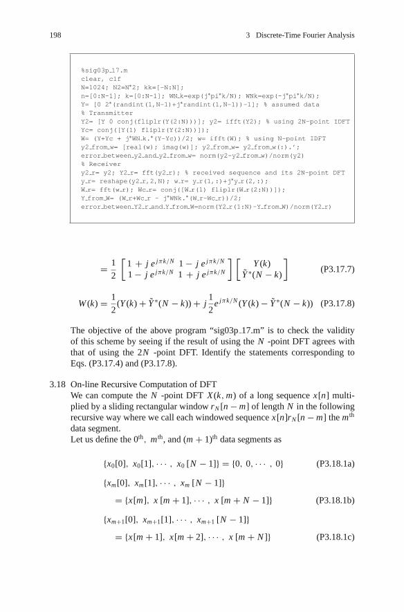
198 3 Discrete-Time Fourier Analysis
%sig03p 17.mclear, clfN=1024; N2=N∗2; kk=[-N:N];n=[0:N-1]; k=[0:N-1]; WN k=exp(j∗pi∗k/N); WNk=exp(-j∗pi∗k/N);Y= [0 2∗(randint(1,N-1)+j∗randint(1,N-1))-1]; % assumed data% TransmitterY2= [Y 0 conj(fliplr(Y(2:N)))]; y2= ifft(Y2); % using 2N-point IDFTYc= conj([Y(1) fliplr(Y(2:N))]);W= (Y+Yc + j∗WN k.∗(Y-Yc))/2; w= ifft(W); % using N-point IDFTy2 from w= [real(w); imag(w)]; y2 from w= y2 from w(:).’;error between y2 and y2 from w= norm(y2-y2 from w)/norm(y2)% Receivery2 r= y2; Y2 r= fft(y2 r); % received sequence and its 2N-point DFTy r= reshape(y2 r,2,N); w r= y r(1,:)+j∗y r(2,:);W r= fft(w r); Wc r= conj([W r(1) fliplr(W r(2:N))]);Y from W= (W r+Wc r - j∗WNk.∗(W r-Wc r))/2;error between Y2 r and Y from W=norm(Y2 r(1:N)-Y from W)/norm(Y2 r)
= 1
2
[1 + j e jπk/N 1 − j e jπk/N
1 − j e jπk/N 1 + j e jπk/N
] [Y (k)
Y ∗(N − k)
](P3.17.7)
W (k) = 1
2(Y (k) + Y ∗(N − k)) + j
1
2e jπk/N (Y (k) − Y ∗(N − k)) (P3.17.8)
The objective of the above program “sig03p 17.m” is to check the validityof this scheme by seeing if the result of using the N -point DFT agrees withthat of using the 2N -point DFT. Identify the statements corresponding toEqs. (P3.17.4) and (P3.17.8).
3.18 On-line Recursive Computation of DFTWe can compute the N -point DFT X (k, m) of a long sequence x[n] multi-plied by a sliding rectangular window rN [n − m] of length N in the followingrecursive way where we call each windowed sequence x[n]rN [n − m] the m th
data segment.Let us define the 0th, m th, and (m + 1)th data segments as
{x0[0], x0[1], · · · , x0 [N − 1]} = {0, 0, · · · , 0} (P3.18.1a)
{xm[0], xm[1], · · · , xm [N − 1]}= {x[m], x [m + 1], · · · , x [m + N − 1]} (P3.18.1b)
{xm+1[0], xm+1[1], · · · , xm+1 [N − 1]}= {x[m + 1], x[m + 2], · · · , x [m + N ]} (P3.18.1c)

Problems 199
Thus we can express the N -point DFT X (k, m + 1) of (m + 1)th data segmentin terms of X (k, m) (i.e., the DFT of the previous segment) as
X (k, m + 1) =∑N−1
n=0xm+1[n] W kn
N =∑N−1
n=0xm [n + 1] W kn
N
=∑N−1
n=0xm [n + 1] W k(n+1)
N W −kN
n+1→ n=∑N
n=1xm[n] W kn
N W −kN
=(∑N−1
n=0xm [n] W kn
N + x[N ] − x [0]
)W −k
N
= (X (k, m) + x [N ] − x [0] ) W −kN (P3.18.2)
Complete the following program “sig03p 18.m” to check the validity. What isthe meaning of “discrepancy” in the program?
%sig03p 18.m% Recursive computation of DFTclear, clfN=64; n=0:N-1; k=0:N-1;W1=2∗pi∗8/N; x=sin(W1∗n);X=fft(x); %FFTxa=[zeros(1,N) x]; % augment x with N zerosXm=zeros(1,N); WN k=exp(j∗2∗pi∗k/N);for m=1:NXm=(Xm+xa(N+m)-xa(m)).∗????; %RDFT
enddiscrepancy= norm(Xm-X)/norm(X)stem(k,abs(Xm)), hold on, pause, stem(k,abs(X),’r’)title(’RDFT and FFT’)
3.19 Two-Dimensional (2-D) DFTTwo-dimensional DFT X (k, l) of a 2-D sequence x[m, n] and its IDFT x[m, n]are defined as
X (k, l) =∑M−1
m=0
∑N−1
n=0x [m, n] W km
M W lnN (P3.19.1a)
for 0 ≤ k ≤ M − 1 and 0 ≤ l ≤ N − 1
x [m, n] = 1
M N
∑M−1
k=0
∑N−1
l=0X (k, l) W −km
M W −lnN (P3.19.1b)
for 0 ≤ m ≤ M − 1 and 0 ≤ n ≤ N − 1
The 2-D DFT can be computed by using a MATLAB built-in function fft2().On the other hand, the 2-D DFT (P3.19.1a) can be written as two cascaded1-D DFTs:

200 3 Discrete-Time Fourier Analysis
X (k, l) =∑M−1
m=0P(m, l) W km
M (P3.19.2a)
for 0 ≤ k ≤ M − 1 and 0 ≤ l ≤ N − 1
with P(m, l) =∑N−1
n=0x [m, n] W ln
N (P3.19.2b)
for 0 ≤ m ≤ M − 1 and 0 ≤ l ≤ N − 1
This implies that the 2-D DFT can be computed by taking the 1-D DFT foreach row of x to get P(m, l) and then taking the 1-D DFT for each columnof P(m, l). Noting that the MATLAB function fft() computes the DFTs ofeach column of the input matrix, compose a program to check the validity ofEq. (P3.19.2a–b) for a 2-D rectangular pulse x[m, n] that is produced and 2-Dor 3-D plotted (in black and white) by the following MATLAB statements:
>>N=64; x=zeros(N,N); x(N/2-3:N/2+3,N/2-5:N/2+5)=255;>>mm=[-N/2:N/2-1]; nn=[-N/2:N/2-1]; image(nn,mm,x) % 2-D plot>>mesh(nn,mm,x), colormap(gray(256)); % Alternatively, 3-D plot
In fact, it does not matter whichever of the column and row is taken the DFTof first.
3.20 Short-Time Fourier Transform (STFT) Using SpectrogramLet us use the MATLAB function spectrogram() to find the STFT for somesignals.
%play music wave.m
clear, clf
Fs=10000; Ts=1/Fs; % 10kHz Sampling Frequency and Sampling period
Tw=2; % Duration of a whole note
melody rhythm= [40 42 44 45 47 49 51 52; 1/4 1/4 1/4 1/4 1/8 1/8 1/8 1/8];
[x,tt]= music wave(melody rhythm,Ts,Tw); sound(x,Fs)
N=256; wnd=N; Noverlap= N/2;
subplot(221), spectrogram(x,wnd,Noverlap,N,Fs,’yaxis’); % specgram(x)
colormap(gray(256)) % colormap(’default’)
function [wave,tt]=music wave(melody rhythm,Ts,Tw)
% Ts: Sampling period, Tw: duration for a whole note
% Copyleft: Won Y. Yang, [email protected], CAU for academic use only
if nargin<3, Tw=2; end
if nargin<2, Ts=0.0001; end
[M,N]= size(melody rhythm);
wave= []; tt=[]; pi2= 2∗pi; phase= 0;
for i=1:N
t= [Ts:Ts:melody rhythm(2,i)∗Tw];if i==1, tt=[tt t]; else tt=[tt tt(end)+t]; end
w= pi2∗440∗2ˆ((melody rhythm(1,i)-49)/12); angle= w∗t + phase;
wave= [wave sin(angle)]; phase= angle(end);
end

Problems 201
The fourth octave
3534 36 38 41 43 46 48 50 53 55 57
37 39 40 42 44 45 47 49 51 52 54 56E5D5C5B4A4G4F4E4D4C4B3
(a) A piano keyboard with the key numbers
(b) A melody written on the music score
treble clef quarter notes eighth notes
A3G3
Fig. P3.20.1
(a) Referring to the above program “play music wave.m” and the layout ofa piano keyboard depicted in Fig. P3.20.1(a), use the MATLAB routine“music wave” to produce a sinusoidal wave for a series of musical notesshown in Fig. P3.20.1(b) where the frequency for the central note A4 is440 Hz and that for any other note is
fn = 440 × 2(n−49)/12[Hz] where n is the key number. (P3.20.1)
(b) Use the MATLAB function “specgram” (in MATLAB of version 6.x) or“spectrogram” (in MATLAB of version 7.x) to find the STFT for thesinusoidal wave produced in (a). You can change the DFT size from itsdefault value N = 256 to 512 and then to 1024 and localize the frequencyrange if you think it to be of help in distinguishing the distinct frequencycomponents. Which of the frequency and time resolutions do you gain orlose by increasing the DFT size?
(c) Beyond the current limit of your ability and the scope of this book, youcan use the RDFT (recursive DFT) or any other technique such as thewavelet transform to improve the time and frequency resolution.
(d) Produce a beat-note signal by summing two sinusoids of slightly differentfrequencies 495 Hz and 505 Hz as
x(t) = cos(2π × 495t) + cos(2π × 505t)
= 2 cos(2π × 500t) cos(2π × 5t) (P3.20.2)
Determine the FFT size (as a power of 2) such that the two frequenciesare distinguishable in the spectrogram. How about the DFT size N whichmakes the frequency resolution
2
N T∼= 505 − 495
2Hz (P3.20.3)

202 3 Discrete-Time Fourier Analysis
where the sampling period T is chosen as 0.0001 s?
2
0
–20
0.02 0.1 t
Fig. P3.20.2 A beat-note signal
(cf.) For example, the spectrogram with N = 512 shows a single fre-quency of around 500 Hz varying in amplitude with time, whilethat with N = 4096 reveals the two different frequencies withconstant amplitude.
3.21 Design of DTMF (Dual-Tone Multi-Frequency) Signal DecoderDTMF system transmits keys pressed on a keypad (Fig. P3.21(a)) through anaudio channel such as a telephone line. Every time a key is pressed, it transmitstwo frequencies, each corresponding to the row and column in which the keyis in.
%sig03p 21.m
% DTMF encoding and decoding
clear, clf
Fs=10000; Ts=1/Fs; % 10kHz Sampling Frequency and Sampling period
keypad.keys= [’1’ ’2’ ’3’ ’A’;
’4’ ’5’ ’6’ ’B’;
’7’ ’8’ ’9’ ’C’;
’*’ ’0’ ’#’ ’D’];
keypad.row freqs= [697 770 852 941];
keypad.col freqs= [1209 1336 1477 1633];
w=2∗pi∗[keypad.row freqs keypad.col freqs];
[x,tt]= dtmf generator(’159D’,[0.1 0.2 0.1 0.2],Ts,keypad);
soundsc(x,Fs)
[keys,B,A]= dtmf decoder(x,Ts,keypad);
keys
sim(’dtmf’,tt(end)); % run the Simulink model file ’dtmf’ for tt(end)[sec]
function [wave,tt]=dtmf generator(keys,durations,Ts,keypad)
% keys, durations : keys pressed and their durations in vectors
% Ts : Sampling period
% Copyleft: Won Y. Yang, [email protected], CAU for academic use only
Nkey= length(keys); Nduration= length(durations);
if Nduration<Nkey
durations= [durations durations(1)∗ones(1,Nkey-Nduration)];end
wave= []; tt=[]; pi2= 2∗pi;Nzero= ceil(0.1/Ts); zero between keys=zeros(1,Nzero);
tzero= [1:Nzero]∗Ts;for i=1:Nkey
t= [Ts:Ts:durations(i)];
if i==1, tt=[tt t];
else tt=[tt tt(end)+t];
end
[m,n]= find(keys(i)==keypad.keys);
if isempty(m), error(’Wrong key in dtmf generator’); end
w2= pi2∗[keypad.row freqs(m); keypad.col freqs(n)];
wave= [wave sum(sin(w2∗t)) zero between keys];
tt=[tt tt(end)+tzero];
end

Problems 203
Coloumn frequencies
Row
freq
uenc
ies 1 2
4 5
7 8
0
(a) A DTMF keypad with the row and column frequencies
∗
3
6
9
A
B
C
D#
697Hz
770Hz
852Hz
941Hz
Number of inputs: 2Multiplication:
Transfer function type: FIRFilter structure: Direct formCoefficient source:
Specify via dialogNumerator coefficients: BInitial conditions: 0
Element-wise(,∗)Sampling time: Ts
Sine type: Time based
Use simulation timeAmplitude: 1, Bias: 0Frequency [rad /sec]: w(1)Phase [rad]: 0Sample time: Ts
Sine Wave Product1
DF FIR
Digital Filter1[Signal Processing /Filtering /Filter Designs]
Digital Filter2
Digital Filter3
Digital Filter4
Digital Filter5
Digital Filter6
Digital Filter7
Digital Filter8
DF FIR
DF FIR
DF FIR
DF FIR
DF FIR
DF FIR
DF FIR
[Simulink [Simulink /Signal Routing]
0
1
–1
0
1
–1
0
0.2
–0.2
0
0.2
–0.2
0
0.5
0.5–0.5
0
0
1
–1
0
1
–1
0
1
–1
1
Mux
[Simulink /Sink]Scope
/Math operations]
×y 1[n ]
d 1[n ]
d 2[n ]
d 3[n ]
d 4[n ]
d 5[n ]
d 6[n ]
d 7[n ]
d 8[n ]
d 1
d 2
d 3
d 4
d 5
d 6
d 7
d 8
y 2[n ]
y 3[n ]
y 4[n ]
y 5[n ]
y 6[n ]
y 7[n ]
y 8[n ]
×
×
×
×
×
×
×
Product2
Product3
Product4
Product5
Product6
Product7
Product8
Sin(ω 1Ts
n)
x (nTs
)
Sin(ω 2Ts
n)
Sin(ω 3Ts
n)
Sin(ω 4Ts
n)
Sin(ω 5Ts
n)
Sin(ω 6Ts
n)
Sin(ω 7Ts
n)
Sin(ω 8Ts
n)
From Workspace[Simulink /Source]
[tt; x].′
Function1
Sine WaveFunction2
Sine WaveFunction3
Sine WaveFunction4
Sine WaveFunction5
Sine WaveFunction6
Sine WaveFunction7
Sine WaveFunction8
Time(t):
1209Hz 1336Hz 1477Hz 1633Hz
(b) The Simulink block diagram for a DTMF decoder
Fig. P3.21
(a) The program “dtmf generator()” listed below generates a DTMF signal(wave) together with the time vector (tt) for given vector (keys) of keyspressed and vector (durations) of key pressing duration. A zero period of0.1 s is inserted between the key signals so that the decoder can distin-guish between a single long-pressed key and multiple repeated keys by

204 3 Discrete-Time Fourier Analysis
accepting a new key only after detecting a zero period. Referring to themain program “sig03p 21.m”, make a DTMF signal for the leading threedigits of your phone number and listen to its sound.
(b) Figure 3.21(b) shows a Simulink block diagram for a filter bank whichcan be used to detect the DTMF signal. In each bank, sin(ωi Tsn) =sin(2π fi Tsn) is multiplied with the input signal where fi = 697, 770, 852,941, 1209, 1336, 1477, and 1633 Hz and the modulated signal is passedthrough a moving or running average filter (MAF). The DTMF signal xtogether with the time vector tt, the sampling period Ts, the analog fre-quency vector w (ωi = 2π fi ’s), and the running average filter coefficientvector B are supposed to be supplied via the MATLAB workspace. Notethat the Simulink model file “dtmf.mdl” can be run directly or indirectlyfrom a MATLAB program by using the MATLAB command “sim()” asillustrated in the program “sig03p 21.m”. Based on the simulation resultsobserved through the scope, determine the common threshold value whichcan be used for detecting any one of the eight frequencies from the output(di [n]) of each MAF.
(c) Complete the following program “dtmf decoder()” and run it on theDTMF signal generated in (a) for demonstration. Note that freqdurations(i) for each frequency is accumulated every sample time thecorresponding MAF output is larger than the threshold value (Thd) andzero duration is increased by one every time no frequency is detected.Whenever the accumulated zero duration exceeds some threshold value(Zero duration) and the frequency durations for at least one of the row fre-quencies and at least one of the column frequencies exceed some threshold(Freq duration), the key corresponding to the row/column frequencies isdetermined.

Problems 205
function [keys,B,A]=dtmf decoder(x,Ts,keypad)% <Inputs> x : Signal vector of DTMF tones% Ts : Sampling period% <Outputs> Keys: Detected key vector% B,A : Numerator/denominator of the filter transfer function% Copyleft: Won Y. Yang, [email protected], CAU for academic use onlyw=2∗pi∗[keypad.row freqs keypad.col freqs]; wTs=w∗Ts;NB=ceil(0.03/Ts); B=ones(1,NB)/NB; A=1; % FIR filter for running averageDCgain= sum(B)/sum(A); B= B/DCgain;NB=length(B); NA=length(A);M=length(wTs); % the input dimension of the filter%wi=zeros(max(NA,NB)-1,M); % the initial stateNx= length(x); tt=[1:Nx]∗Ts; % the length of signal and the time vectory=[]; d=[]; keys= [];freq durations=zeros(1,M); zero duration=0; Thd=0.1;Zero duration= 0.08/Ts; Freq duration= 0.09/Ts;for n=1:Nx
y= [y; x(n)∗sin(wTs∗n)];if n==1, [dn,wi]= filter(B,A,[zeros(1,M); y(end,:)]); % column-wiseelse [dn,wi]= filter(B,A,y([end-1 end],:),wi); % multi-filteringendd = [d; dn(end,:)]; tmp = (abs(dn(end,:))>Thd);freq durations = freq durations + tmp;zero duration = zero duration + (sum(tmp)==0);cond1= (zero duration>Zero duration);cond2= sum(freq durations(1:4)>Freq duration)>0;cond3= sum(freq durations(5:8)>Freq duration)>0;if cond1&cond2&cond3?????????????????????????????????????????????????????????????????????????????????????????????????????????????????????????????????????????????????????????????????????end
end
Chapter 4The z-Transform
Contents
4.1 Definition of the z-Transform . . . . . . . . . . . . . . . . . . . . . . . . . . . . . . . . . . . . . . . . . . . . . . . . 2084.2 Properties of the z-Transform . . . . . . . . . . . . . . . . . . . . . . . . . . . . . . . . . . . . . . . . . . . . . . . . 213
4.2.1 Linearity . . . . . . . . . . . . . . . . . . . . . . . . . . . . . . . . . . . . . . . . . . . . . . . . . . . . . . . . . . 2134.2.2 Time Shifting – Real Translation . . . . . . . . . . . . . . . . . . . . . . . . . . . . . . . . . . . . . . 2144.2.3 Frequency Shifting – Complex Translation . . . . . . . . . . . . . . . . . . . . . . . . . . . . . . 2154.2.4 Time Reversal . . . . . . . . . . . . . . . . . . . . . . . . . . . . . . . . . . . . . . . . . . . . . . . . . . . . . . 2154.2.5 Real Convolution . . . . . . . . . . . . . . . . . . . . . . . . . . . . . . . . . . . . . . . . . . . . . . . . . . . 2154.2.6 Complex Convolution . . . . . . . . . . . . . . . . . . . . . . . . . . . . . . . . . . . . . . . . . . . . . . . 2164.2.7 Complex Differentiation . . . . . . . . . . . . . . . . . . . . . . . . . . . . . . . . . . . . . . . . . . . . . 2164.2.8 Partial Differentiation . . . . . . . . . . . . . . . . . . . . . . . . . . . . . . . . . . . . . . . . . . . . . . . 2174.2.9 Initial Value Theorem . . . . . . . . . . . . . . . . . . . . . . . . . . . . . . . . . . . . . . . . . . . . . . . 2174.2.10 Final Value Theorem . . . . . . . . . . . . . . . . . . . . . . . . . . . . . . . . . . . . . . . . . . . . . . . . 218
4.3 The Inverse z-Transform . . . . . . . . . . . . . . . . . . . . . . . . . . . . . . . . . . . . . . . . . . . . . . . . . . . . 2184.3.1 Inverse z-Transform by Partial Fraction Expansion . . . . . . . . . . . . . . . . . . . . . . . 2194.3.2 Inverse z-Transform by Long Division . . . . . . . . . . . . . . . . . . . . . . . . . . . . . . . . . . 223
4.4 Analysis of LTI Systems Using the z-Transform . . . . . . . . . . . . . . . . . . . . . . . . . . . . . . . . 2244.5 Geometric Evaluation of the z-Transform . . . . . . . . . . . . . . . . . . . . . . . . . . . . . . . . . . . . . . 2314.6 The z-Transform of Symmetric Sequences . . . . . . . . . . . . . . . . . . . . . . . . . . . . . . . . . . . . . 236
4.6.1 Symmetric Sequences . . . . . . . . . . . . . . . . . . . . . . . . . . . . . . . . . . . . . . . . . . . . . . . 2364.6.2 Anti-Symmetric Sequences . . . . . . . . . . . . . . . . . . . . . . . . . . . . . . . . . . . . . . . . . . . 237
4.7 Summary . . . . . . . . . . . . . . . . . . . . . . . . . . . . . . . . . . . . . . . . . . . . . . . . . . . . . . . . . . . . . . . . . 240Problems . . . . . . . . . . . . . . . . . . . . . . . . . . . . . . . . . . . . . . . . . . . . . . . . . . . . . . . . . . . . . . . . . 240
The z-transform is the discrete-time counterpart of the Laplace transform. It can beviewed as a generalization of the DTFT (discrete-time Fourier transform) just as theLaplace transform can be viewed as a generalization of the CTFT (continuous-timeFourier transform). It plays a vital role in the analysis and design of discrete-timelinear time-invariant (LTI) systems that are described by difference equations. Inthis chapter we introduce the z-transform and discuss some of its properties andapplications to LTI system analysis and representations.
W.Y. Yang et al., Signals and Systems with MATLAB R©,DOI 10.1007/978-3-540-92954-3 4, C© Springer-Verlag Berlin Heidelberg 2009
207

208 4 The z-Transform
4.1 Definition of the z-Transform
For a discrete-time sequence x[n], the bilateral (two-sided) and unilateral (one-sided) z-transforms are defined as
X [z] = Z{x[n]} =∑∞
n=−∞ x[n]z−n
(4.1.1a)X [z] = Z{x[n]} =
∑∞n=0
x[n]z−n
(4.1.1b)
where z is a complex variable. For convenience, the z-transform relationship willsometimes be denoted as
x[n]Z↔ X [z] x[n]
Z↔ X [z]
Note that the unilateral z-transform of x[n] can be thought of as the bilateralz-transform of x[n]us[n] (us[n]: the unit step sequence) and therefore the twodefinitions will be identical for causal sequences. The unilateral z-transform is par-ticularly useful in analyzing causal systems described by linear constant-coefficientdifference equations with initial conditions.
The z-transform does not necessarily exist for all values of z in the complexplane. For the z-transform to exist, the series in Eq. (4.1.1) must converge. For agiven sequence x[n], the domain of the z-plane within which the series converges iscalled the region of convergence (ROC) of the z-transform X[z] or X [z]. Thus, thespecification of the z-transform requires both the algebraic expression in z and itsregion of convergence.
Note that a sequence x[n] is called
– a right-sided sequence if x[n] = 0 ∀ n < n0 for some finite integer n0,– a causal sequence if x[n] = 0 ∀ n < n0 for some nonnegative integer n0 ≥ 0,– a left-sided sequence if x[n] = 0 ∀ n ≥ n0 for some finite integer n0, and– a anti-causal sequence if x[n] = 0 ∀ n ≥ n0 for some non-positive integer
n0 ≤ 0,
respectively.
Example 4.1 The z-Transform of Exponential Sequences
(a) For a right-sided and causal sequence x1[n] = anus[n], we can use Eq. (4.1.1a)to get its bilateral z-transform as
X1[z] = Z{x1[n]} =∑∞
n=−∞ anus[n]z−n =∑∞
n=0anz−n
(D.23)= 1
1 − az−1= z
z − a(E4.1.1)
This geometric sequence converges for |az−1| < 1, which implies that the ROCof X1[z] is R1 = {z : |z| > |a|} (see Fig. 4.1(a)).

4.1 Definition of the z-Transform 209
(a) ROC for a right-sided sequence
(b) ROC for a left-sided sequence
(c) ROC for a both-sided sequence
R2 = {z: |z | < |b |}R1 = {z: |z | > |a |} R = R1 ∩ R2 = {z: |a | < |z | < |b |}
Re {z}|a|0
Im {z} Im {z}
0 Re {z}|a| |b||b|
Im {z}
Re {z}0
Fig. 4.1 Three forms of ROC (region of convergence)
(b) For a left-sided and anti-causal sequence x2[n] = −bnus[−n − 1], we can useEq. (4.1.1a) to get its bilateral z-transform as
X2[z] = Z{x2[n]} =∑∞
n=−∞ −bnus[−n − 1]z−n = −∑−1
n=−∞ bnz−n
= −∑∞
n=1(b−1z)n (D.23)= −b−1z
1 − b−1z= z
z − b(E4.1.2)
This geometric sequence converges for |b−1z| < 1, which implies that the ROCof X2[z] is R2 = {z : |z| < |b|} (see Fig. 4.1(b)).
(c) For the both-sided sequence
y[n] = x1[n] + x2[n] = anus[n] − bnus[−n − 1] (E4.1.3)
we can combine the above results of (a) and (b) to obtain its bilateral z-transform as
Y[z] = X1[z] + X2[z] = z
z − a+ z
z − b(E4.1.4)
For this series to converge, both of the two series must converge and therefore,its ROC is the intersection of the two ROCs R1 and R2 : R = R1 ∩ R2 ={z : |a| < |z| < |b|}. This is an annular region |a| < |z| < |b| (Fig. 4.1(c)) if|b| > |a| and it will be an empty set if |b| ≤ |a|.
(cf) This example illustrates that different sequences may have the same z-transform,but with different ROCs. This implies that a z-transform expression maycorrespond to different sequences depending on its ROC.
Remark 4.1 Region of Convergence (ROC)
(1) The ROC for X [z] is an annular ring centered at the origin in the z-plane ofthe form

210 4 The z-Transform
r− < |z| < r+ (4.1.2)
where r+ can be as large as ∞ (Fig. 4.1(a)) for causal sequences and r− can beas small as zero (Fig. 4.1(b)) for anti-causal sequences.
(2) As illustrated in Example 4.1, the three different forms of ROC shown inFig. 4.1 can be associated with the corresponding three different classes ofdiscrete-time sequences; 0 < r− < |z| for right-sided sequences, |z| < r+ < ∞for left-sided sequences, and r− < |z| < r+ (annular ring) for two-sidedsequences.
Example 4.2 A Causal Sequence Having Multiple-Pole z-transformFor a sum of two causal sequences
x[n] = x1[n] + x2[n] = 2us[n] − 2(1/2)nus[n] (E4.2.1)
we can use Eq. (E4.1.1) to get the z-transform for each sequence and combine thez-transforms as
X[z] = Z{x[n]} = X1[z] + X2[z](E4.1.1)=
with a=1 and a=1/22
z
z − a
∣∣∣∣a=1
−2z
z − a
∣∣∣∣a=1/2
= 2z
z − 1− 2z
z − 1/2= z
(z − 1)(z − 1/2)(E4.2.2)
Since both X1[z] = Z{x1[n]} and X2[z] = Z{x2[n]} must exist for this z-transformto exist, the ROC is the intersection of the ROCs for the two z-transforms:
R = R1 ∩ R2 = {z : |z| > 1} ∩ {z : |z| > 1/2} = {z : |z| > 1} (E4.2.3)
(cf) Figure 4.2 shows the pole-zero pattern of the z-transform expression (E4.2.2)where a pole and a zero are marked with x and o, respectively. Note that theROC of the z-transform X[z] of a right-sided sequence is the exterior of thecircle which is centered at the origin and passes through the pole farthest fromthe origin in the z-plane.
Fig. 4.2 Pole-zero pattern ofthe z-transform (E4.2.2)
Im{z}
Re{z}11/2
z-plane
× ×

4.1 Definition of the z-Transform 211
Before working further with more examples, let us see the relationship betweenthe z-transform and DTFT (discrete-time Fourier transform), which is summarizedin the following remark:
Remark 4.2 The z-Transform and the DTFT (Discrete-Time Fourier Transform)Comparing the bilateral z-transform (4.1.1a) with the DTFT (3.1.1), we can see
their relationship that the DTFT can be obtained by substituting z = e jΩ into the(bilateral) z-transform:
F{x[n]} = X ( jΩ)(3.1.1)=
∑∞n=−∞ x[n]e− jΩn = X [e jΩ]
= X [z]|z=e jΩ = Z{x[n]}|z=e jΩ (4.1.3)
This implies that the evaluation of the z-transform along the unit circle in the z-plane yields the DTFT. Therefore, in order for the DTFT to exist, the ROC of thez-transform must include the unit circle (see Fig. 4.3).
Example 4.3 The z-transform of a Complex Exponential SequenceLet us consider a causal sequence
x[n] = e jΩ1nus[n] = cos(Ω1n)us[n] + j sin(Ω1n)us[n] (E4.3.1)
We can find the z-transform of this exponential sequence by substituting a = e jΩ1
into Eq. (E4.1.1) as
X[z] = Z{e jΩ1nus[n]} (E4.1.1)=a=e jΩ1
z
z − e jΩ1= z(z − e− jΩ1 )
(z − e jΩ1 )(z − e− jΩ1 ), |z| > |e± jΩ1 | = 1;
e jΩ1nus[n](D.20)= cos(Ω1n)us[n] + j sin(Ω1n)us[n]
Z↔ z(z − cos Ω1)
z2 − 2z cos Ω1 + 1+ j
z sin Ω1
z2 − 2z cos Ω1 + 1
Fig. 4.3 The relationshipbetween the DTFT andz-transform
Re{z}
Im{z}
F{x[n]} = X( jΩ) = (X [z] = Z{x [n]}) with z = e jΩ
0 1
z-plane
z = e jΩ
Ω

212 4 The z-Transform
This implies the following two z-transform pairs:
cos(Ω1n)us[n]Z↔ z(z − cos Ω1)
z2 − 2z cos Ω1 + 1= z(z − cos Ω1)
(z − cos Ω1)2 + sin2 Ω1(E4.3.2)
with R = {z : |z| > 1}sin(Ω1n)us[n]
Z↔ z sin Ω1
z2 − 2z cos Ω1 + 1= z sin Ω1
(z − cos Ω1)2 + sin2 Ω1(E4.3.3)
with R = {z : |z| > 1}
Example 4.4 The z-transform of an Exponentially Decreasing Sinusoidal SequenceFor a causal sequence
x[n] = rn cos(Ω1n)us[n](D.21)= 1
2rn(e jΩ1n + e− jΩ1n)us[n] (E4.4.1)
we can use Eq. (E4.1.1) with a = e± jΩ1 to find the z-transform of this sequence as
X[z](E4.1.1)=
a=re jΩ1 and a=re− jΩ1
1
2
(z
z − re jΩ1+ z
z − re− jΩ1
)= z(z − r cos Ω1)
z2 − 2zr cos Ω1 + r2
(E4.4.2)
where the ROC is R = {z : |z| > |r e± jΩ1 | = |r |}.
(cf) Note that if |r | ≥ 1, the ROC does not contain the unit circle and consequently,the DTFT does not exist in the strict sense.
We could elaborate on more examples of the z-transform computation. However,we instead list a number of useful z-transform pairs in Table B.9 in Appendix B sothat the readers can use them for finding the z-transform or inverse z-transform.
In many cases, we deal with the z-transform that is expressed in the form of arational function, i.e., a ratio of polynomials in z. For such a rational z-transformX[z] = Q[z]/P[z], we define its singularities, i.e., poles and zeros as follows:
Remark 4.3 Poles and Zeros of a Rational z-Transform Expression X[z] = Q[z]/P[z]
The roots of Q[z] = 0, or the values of z at which X[z] = 0 are called thezeros of X[z]. The poles are the roots of P[z] = 0, or the values of z for whichX[z] = ∞. If we count the singularities at z = ∞, the number of poles will beequal to that of zeros. Notice that, for polynomials with real-valued coefficients, thecomplex-valued singularities must occur in complex-conjugate pairs.
The ROC of a z-transform X[z] can be described in terms of its poles as follows:

4.2 Properties of the z-Transform 213
Remark 4.4 Pole Locations and Region of Convergence (ROC)
(1) It is obvious that there can be no poles of a z-transform X[z] inside the ROCsince the z-transform does not converge at its poles. In fact, the ROC is boundedby poles or infinity as illustrated by Examples 4.1 and 4.2.
(2) For a right-sided sequence xa[n] and left-sided sequence xb[n], the ROCs fortheir z-transforms Xa[z] and Xb[z] are outside/inside the outermost/innermostpole, respectively:
R1 = {z : |z| > the maximum of |ai |′s}(z = ai : the poles of Xa[z]) (4.1.4a)
(as illustrated by Example 4.2) or
R2 = {z : |z| < the minimum of |bi |′s}(z = bi : the poles of Xb[z]) (4.1.4b)
For a two-sided sequence x[n] = x[n] + xb[n], the ROC is an annular regiongiven by
R = R1 ∩ R2 = {z : maxi
|ai | < |z| < minj
|b j |} (4.1.4c)
4.2 Properties of the z-Transform
In this section we discuss the properties of the z-transform that are useful in obtain-ing z-transform pairs and in applying the transform to the analysis of discrete-timelinear time-invariant systems. These properties are very similar to those of theLaplace transform and Fourier transform.
Most of the properties are commonly applicable to the bilateral and unilateralz-transforms. There are, however, a few exceptions such as the time shifting prop-erty, time reversal property, and initial/final value theorems. In particular, it is thetime shifting property that makes the unilateral z-transform very useful for solvingdifference equations with initial conditions.
4.2.1 Linearity
Let the z-transforms of two time sequences x[n] and y[n] be Z{x[n]} = X[z] withROC Rx and Z{y[n]} = Y[z] with ROC Ry . Then we can express the z-transformof their linear combination in terms of X[z] and Y[z] as
ax[n] + βy[n]z↔ αX[z] + βY[z] with ROC R ⊃ (R1 ∩ R2) (4.2.1)
where the ROC is generally the intersection of the two ROCs Rx and Ry , but it canbe larger when any pole of X[z] and Y[z] is cancelled by the zeros resulting fromthe addition.
214 4 The z-Transform
4.2.2 Time Shifting – Real Translation
Let the bilateral z-transform of x[n] be Z{x[n]} = X[z] with ROC Rx . Then thebilateral z-transform of a time-shifted version x[n − n1] is
x[n − n1]z↔ z−n1X[z], ROC Rx (possibly with z = 0 or ∞ added or removed)
(4.2.2)
The addition/removal of z = ∞ to/from the ROC occurs when a causal/non-causalsequence is shifted to become a non-causal/causal sequence. Similarly, the addi-tion/removal of the origin z = 0 to/from the ROC is owing to the possible transitionbetween anticausal and non-anticausal sequences resulting from the shift operation.
On the other hand, the time-shifting property of the unilateral z-transform is asfollows:
<Case 1> x[n − n1], n1 > 0 (delayed sequence)
Z{x[n − n1]} =∑∞
n=0x[n − n1]z−n
=∑n1−1
n=0x[n − n1]z−n +
∑∞n=n1
x[n − n1]z−n
n−n1=m,n=m+n1=∑−1
m=−n1x[m]z−(m+n1) +
∑∞m=0
x[m]z−(m+n1)
= z−n1
(∑∞m=0
x[m]z−m +∑−1
m=−n1x[m]z−m
);
x[n − n1]Z↔ z−n1
(X [z] +
∑−1
m=−n1x[m]z−m
)(4.2.3a)
where the second term in the RHS will disappear when x[n] is causal.
<Case 2> x[n + n1], n1 > 0 (advanced sequence)
Z{x[n + n1]} =∑∞
n=0x[n + n1]z−n n+n1=m,n=m−n1=
∑∞n=n1
x[m]z−(m−n1)
= zn1
(∑∞m=0
x[m]z−m −∑n1−1
m=0x[m]z−m
);
x[n + n1]Z↔ zn1
(X [z] −
∑n1−1
m=0x[m]z−m
)(4.2.3b)
Example 4.5 Applying Linearity and Time Shifting Properties of the z-TransformFor a rectangular pulse sequence of duration N given by
x[n] = us[n] − us[n − N ] =n=···−1 0 1 ···N−1 N ···{· · · 0 1 1 · · · 1 0 · · · } (E4.5.1)

4.2 Properties of the z-Transform 215
we can use Eq. (E4.1.1) (with a = 1) together with the linearity (4.2.1) and time-shifting property (4.2.2) to get its z-transform as
X[z](E4.1.1) with a=1=
(4.2.1)&(4.2.2)
z
z − 1− z−N z
z − 1= zN − 1
zN−1(z − 1)(E4.5.2)
Note that X[z] has multiple pole of order N − 1 at z = 0 and N − 1 zeros atz = e j2mπ/N (for m = 1, 2, · · · , N − 1) on the unit circle where the zero at z = 1(resulting from the addition) cancels the pole (of Z{us[n]} = z/(z −1)) at that point.Due to this pole-zero cancellation, the ROC of X[z] becomes |z| > 0 (the entirez-plane except the origin z = 0), which is larger than that of Z{us[n]} = z/(z − 1),i.e., |z| > 1.
4.2.3 Frequency Shifting – Complex Translation
Let the bilateral z-transform of x[n] be Z{x[n]} = X[z] with ROC Rx = {z :r−
x < |z| < r+x }. Then we have the z-transform of a frequency-shifted or modulated
version zn1 x[n] as
e jΩ1n x[n]z↔ X[e− jΩ1 z] with ROC : Rx = {z : r−
x < |z| < r+x } (4.2.4a)
zn1 x[n]
z↔ X[z/z1] with ROC : |z1|Rx = {z : |z1|r−x < |z| < |z1|r+
x } (4.2.4b)
4.2.4 Time Reversal
Let the bilateral z-transform of x[n] be Z{x[n]} = X[z] with ROC Rx = {z :r−
x < |z| < r+x }. Then we have the bilateral z-transform of a time-reversed version
x[−n] as
x[−n]z↔ X[z−1] with ROC : 1/Rx = {z : 1/r+
x < |z| < 1/r−x } (4.2.5)
where if z ∈ Rx , then 1/z ∈ 1/Rx .
4.2.5 Real Convolution
Let the z-transforms of two time sequences g[n] and x[n] be Z{g[n]} = G[z] withROC Rg and Z{x[n]} = X[z] with ROC Rx . Then we can express the z-transformof their convolution in terms of G[z] and X[z] as
y[n] = g[n] ∗ x[n]z↔ Y[z] = G[z] X[z] with ROC R ⊃ (Rg ∩ Rx ) (4.2.6)
216 4 The z-Transform
(proof)
Z{g[n] ∗ x[n]} (4.1.1a)=∑∞
n=−∞ (g[n] ∗ x[n])z−n
(1.2.9)=∑∞
n=−∞
(∑∞m=−∞ g[m]x[n − m]
)z−n
=∑∞
m=−∞
(g[m]
∑∞n=−∞ x[n − m]z−(n−m)z−m
)n−m→n, n→n+m=
∑∞m=−∞
(g[m]z−m
∑∞n=−∞ x[n]z−n
)(4.1.1a)= G[z]X[z]
This convolution property holds for causal sequences, which implies that the uni-lateral z-transform also has the same property. It is very useful for describing theinput-output relationship of a discrete-time LTI system with the input x[n], out-put y[n], and impulse response g[n] where the transform of the impulse response,Z{g[n]} = G[z], is called the system or transfer function (see Sects. 1.2.3 and 1.2.4).
4.2.6 Complex Convolution
Let the z-transforms of x[n] and y[n] be Z{x[n]} = X[z] with ROC Rx = {z : r−x <
|z| < r+x } and Z{y[n]} = Y[z] with ROC Ry = {z : r−
y < |z| < r+y }, respectively.
Then the z-transform of the product of the two sequences can be expressed in termsof X[z] and Y[z] as
x[n]y[n]Z↔ 1
2π j
∮C1
X[z/v]Y[v]v−1dv with ROC R = {z : r−x r−
y < |z| < r+x r+
y }(4.2.7a)
x[n]y[n]Z↔ 1
2π j
∮C2
X[v]Y[z/v]v−1dv with ROC R = {z : r−x r−
y < |z| < r+x r+
y }(4.2.7b)
where∮
Cimeans the complex integral along a closed contour Ci within the intersec-
tion of the ROCs of X[z/v] and Y[v] or X[v] and Y[z/v] (see [O-2], Sect. 2.3.9 forits proof).
4.2.7 Complex Differentiation
Let the z-transform of x[n] be Z{x[n]} = X[z] with ROC Rx . Then the z-transformof nx[n] can be expressed in terms of X[z] as
nx[n]Z↔ −z
d
dzX[z] with ROC Rx (4.2.8)

4.2 Properties of the z-Transform 217
This can be proved by differentiating the definition of the z-transform (4.1.1)w.r.t. z.
4.2.8 Partial Differentiation
If a z-transform pair is given in the form of Z{x(nT, a)} = X(z, a) with a parametera, we can differentiate it w.r.t. a to obtain another z-transform pair as
∂
∂ax(nT, a)
Z↔ ∂
∂aX (z, a) (4.2.9)
Example 4.6 Complex Differentiation and Partial DifferentiationFor y[n] = n2anus[n], we can apply the complex differentiation property (4.2.8)
twice for Eq. (E4.1.1) to write
nanus[n]Z↔ −z
d
dz
(z
z − a
)= −z
(z − a) − z
(z − a)2= az
(z − a)2(E4.6.1)
n2anus[n]Z↔ −z
d
dz
(az
(z − a)2
)= −z
a(z − a)2 − 2az(z − a)
(z − a)4= az(z + a)
(z − a)3
(E4.6.2)
Alternatively, we can apply the partial differentiation property for Eq. (E4.1.1) toget the same results:
nan−1us[n]Z↔ ∂
∂a
(z
z − a
)= z
(z − a)2(E4.6.3)
n2an−1us[n]Z↔ ∂
∂a
(az
(z − a)2
)= z(z − a)2 + 2az(z − a)
(z − a)4= z(z + a)
(z − a)3(E4.6.4)
Multiplying both sides of these equations by a yields Eqs. (E4.6.1) and (E4.6.2),which are listed in Table B.9(10) and (12).
4.2.9 Initial Value Theorem
For a causal sequence x[n] such that x[n] = 0 ∀ n < 0, we can get its initial valuex[0] from its z-transform as
x[0] = limz→∞ X [z] (4.2.10)
This can easily be shown by substituting z = ∞ into the z-transform definition(4.1.1b).

218 4 The z-Transform
4.2.10 Final Value Theorem
For a causal sequence x[n] such that x[n] = 0 ∀ n < 0, we can get its final valuex[∞] from its z-transform as
x[∞] = limz→1
(z − 1)X [z] = limz→1
(1 − z−1)X [z] (4.2.11)
This requires that x[n] should converge or equivalently, all the poles of its z-transform X [z] should lie inside the unit circle possibly with the exception of asimple pole at z = 1.(proof)
We can use the z-transform definition (4.1.1b) to write
Z{x[n + 1] − x[n]} = limk→∞
(∑k
n=0x[n + 1]z−n −
∑k
n=0x[n]z−n
)
= limk→∞
(∑k
n=1x[n]z−(n−1) + x[k + 1]z−k
− x[0] −∑k
n=1x[n]z−n
)
On the other hand, from the time shifting property (4.2.3b), we can write
Z{x[n + 1] − x[n]} (4.2.1)= Z{x[n + 1]} − Z{x[n]}(4.2.3)= z(X [z] − x[0]) − X [z] = (z − 1)X [z] − zx[0]
Noting that these two equations are commonly the z-transform of (x[n + 1] − x[n]),we can equate their RHSs and substitute z = 1 to get the desired result.
4.3 The Inverse z-Transform
In this section we consider how to find x[n] for a given z-transform X [z] with itsROC. From the complex variable theory, the inverse z-transform formula can bederived (see [O-2], Sect. 2.2) as
x[n] = 1
2π j
∮C
X[z]z−ndz (4.3.1)
where∮
C means the complex integral along a closed contour C within the ROCof X[z] encircling the origin of the z-plane in the counterclockwise direction. It is,however, difficult to directly evaluate this integral and therefore we make resort toalternative procedures for obtaining the inverse z-transform.

4.3 The Inverse z-Transform 219
4.3.1 Inverse z-Transform by Partial Fraction Expansion
Noting that the complex variable z appears in the numerator of almost every basicz-transform listed in Table B.9, we apply the same procedure as with the inverseLaplace transform (Sect. A.4) to get the partial fraction expansion on X [z]/z andthen multiply both sides by z so that we can directly use the z-transform table to getthe inverse z-transform.
More specifically, let X [z]/z be rational as
X [z]
z= Q1[z]
P[z]= bM zM + . . . + b1z + b0
aN zN + . . . + a1z + a0(4.3.2)
where M and N are the degrees of the numerator and denominator polynomials,respectively. If M ≥ N , we divide Q1[z] by P[z] starting with the highest powersof z to produce the remainder polynomial of degree less than N :
X [z]
z= Q[z]
P[z]+ cM−N zM−N + . . . + c1z + c0 (4.3.3)
If M < N , we have only the first term on the RHS where ci = 0 for all i . Now,for the purpose of illustration, we assume that all the poles of Q[z]/P[z] are simpleexcept one multiple pole of order L at z = p so that we can write Q[z]/P[z] in thefollowing form:
Q[z]
P[z]=(
N−L∑i=1
ri
z − pi
)+ rN−L+1
z − p+ . . . + rN
(z − p)L+ K (4.3.4)
where
ri = (z − pi )Q[z]
P[z]
∣∣∣∣ z = pi, i = 1, 2, . . . , N − L (4.3.5a)
rN−l = 1
l!
dl
dzl
{(z − p)L Q[z]
P[z]
} ∣∣∣∣ z = p, l = 0, 1, . . . , L − 1 (4.3.5b)
Now, substituting Eq. (4.3.4) into Eq. (4.3.3), multiplying the both sides by z, andusing the z-transform Table B.9, we can obtain the inverse z-transform of X [z] as
x[n] ={
N−L∑i=1
ri pni + rN−L+1 pn + rN−L+2npn−1 + . . .
+ rNn!
(L − 1)!(n − L + 1)!pn−L+1
}us[n] +
M−N∑i=0
ciδ[n + i + 1] (4.3.6)
220 4 The z-Transform
Example 4.7 The Inverse z-Transform by Partial Fraction Expansion
(a) Let us find the inverse z-transform of
X [z] = z
z3 − 2z2 + (5/4)z − 1/4= z
(z − 1)(z − 1/2)2(E4.7.1)
with ROC R = {z : |z| > 1}
We first divide this by z and then expand it into partial fractions:
X [z]
z= r1
z − 1+ r2
z − 1/2+ r3
(z − 1/2)2
(4.7.3)= 4
z − 1− 4
z − 1/2− 2
(z − 1/2)2(E4.7.2)
where the coefficient of each term can be found from Eq. (4.3.5) as
r1(4.3.5a)= (z − 1)
X [z]
z
∣∣∣∣z=1
= 4 (E4.7.3a)
r2(4.3.5b)=
l=1
d
dz
((z − 1/2)2 X [z]
z
)∣∣∣∣z=1/2
= d
dz
(1
z − 1
)∣∣∣∣z=1/2
= − 1
(z − 1)2
∣∣∣∣z=1/2
= −4 (E4.7.3b)
r3(4.3.5b)=
l=0(z − 1/2)2 X [z]
z
∣∣∣∣z=1/2
= 1
z − 1
∣∣∣∣z=1/2
= −2 (E4.7.3c)
Now, moving the z (which we have saved) from the LHS back into the RHSyields
X [z] = 4z
z − 1− 4
z
z − 1/2− 4
(1/2)z
(z − 1/2)2(E4.7.4)
Then we can use Table B.9(3), (5), and (10) to write the inverse z-transform as
x[n] =(
4 − 4
(1
2
)n
− 4n
(1
2
)n)us[n] (E4.7.5)
where the right-sided sequences are chosen over the left-sided ones since thegiven ROC is not the inside, but the outside of a circle.We can use the MATLAB command ‘residue( )’ or ‘residuez( )’ to get the par-tial fraction expansion and ‘iztrans( )’ to obtain the whole inverse z-transform.

4.3 The Inverse z-Transform 221
It should, however, be noted that ‘iztrans()’ might not work properly for high-degree rational functions.
>>Nz=[0 1]; Dz=poly([1 1/2 1/2]), [r,p,k]=residue(Nz,Dz); [r p],k %(E4.7.2)r = 4.0000 p = 1.0000 % (E4.7.3a) 4/(z-1)
-4.0000 0.5000 % (E4.7.3b) -4/(z-0.5)-2.0000 0.5000 % (E4.7.3c) -2/(z-0.5)ˆ2
k = []>>syms z, x=iztrans(z/(zˆ3-2*zˆ2+1.25*z-0.25)) % (E4.7.1)
x = 4-4*(1/2)ˆn-4*(1/2)ˆn*n % (E4.7.5)
(b) Let us find the inverse z-transform of
X [z] = 3z
z2 − (1/4)z − 1/8= 3z
(z − 1/2)(z + 1/4)(E4.7.6)
with one of the following three ROCs:
R1 ={
z : |z| >1
2
},R2 =
{z : |z| <
1
4
}, and
R3 ={
z :1
4< |z| <
1
2
}(E4.7.7)
We first divide this by z and then expand it into partial fractions:
X [z]
z= 4
z − 1/2− 4
z + 1/4; X [z] = 4
z
z − 1/2− 4
z
z + 1/4(E4.7.8)
Now, depending on the ROC, we use Table B.9(5) or (6) to write the inversez-transform as follows:
(i) R1 ={
z : |z| >1
2
}: x[n] = 4
(1
2
)n
us[n] − 4
(−1
4
)n
us[n]
(E4.7.9a)
(ii) R2 ={
z : |z| <1
4
}:
x[n] = −4
(1
2
)n
us[−n − 1] + 4
(−1
4
)n
us[−n − 1] (E4.7.9b)
(iii) R3 ={
z :1
4< |z| <
1
2
}:
x[n] = −4
(1
2
)n
us[−n − 1] − 4
(−1
4
)n
us[n] (E4.7.9c)
>>syms z, x=iztrans(3*z/(zˆ2-0.25*z-1/8)) % (E4.7.6)x = 4*(1/2)ˆn-4*(-1/4)ˆn % (E4.7.9a) just a right-sided sequence
222 4 The z-Transform
Example 4.8 The Inverse z-Transform by Partial Fraction ExpansionLet us find the inverse z-transform of
X [z] = 2z2
z2 − z + 1/2= 2z2
(z − 0.5 − j0.5)(z − 0.5 + j0.5)(E4.8.1)
with ROC R = {z : |z| > 1}
We first divide this by z and then expand it into partial fractions:
X [z]
z= rR + jrI
z − 0.5 − j0.5+ rR − jrI
z − 0.5 + j0.5
= 1 − j
z − 0.5 − j0.5+ 1 + j
z − 0.5 + j0.5(E4.8.2)
Now, moving the z (which we have saved) from the LHS back into the RHS yields
X [z] = (1 − j)z
z − 0.5 − j0.5+ (1 + j)z
z − 0.5 + j0.5(E4.8.3)
We can use Table B.9(5) to write the inverse z-transform as
x[n] = (1 − j)(0.5 + j0.5)nus[n] + (1 + j)(0.5 − j0.5)nus[n]
=√
2(
e− jπ/4√
2−n
e jnπ/4 + e jπ/4√
2−n
e− jnπ/4)
us[n]
=√
2−n+3
cos((n − 1)π
4)us[n] (E4.8.4)
As a nice alternative for X [z] having complex conjugate poles like (E4.8.1), we candecompose it into the following form, which can be matched exactly with someelement of the z-transform table:
X [z] = 2z(z − 1/2)
(z − 1/2)2 + (1/2)2+ 2(1/2)z
(z − 1/2)2 + (1/2)2
= 2z(z − r cos Ω1)
(z − r cos Ω1)2 + r2 sin2 Ω1+ 2
zr sin Ω1
(z − r cos Ω1)2 + r2 sin2 Ω1(E4.8.5)
where r = 1/√
2, cos Ω1 = 1/√
2, sin Ω1 = 1/√
2, and Ω1 = π/4. Then we canuse B.9(18) and (17) to obtain the same result as (E4.8.3):
x[n] = 2(rn cos(Ω1n) + rn sin(Ω1n)
)us[n]
= 2(√
2−n
cos(π
4n) +
√2
−nsin(
π
4n))
us[n]
=√
2−n+3
cos((n − 1)π
4)us[n] =
√2
−n+3sin((n + 1)
π
4)us[n] (E4.8.6)

4.3 The Inverse z-Transform 223
(cf) It seems that the MATLAB command ‘iztrans()’ does not work properly forthis problem:
>>syms z, x=iztrans(2*zˆ2/(zˆ2-z+1/2)) % (E4.8.1)>>n=1:10; xn=2.ˆ(-(n-3)/2).*cos((n-1)*pi/4); stem(n,xn), hold on %(E4.8.6)>>[r,p,k]=residuez([2 0 0],[1 -1 1/2]) % Partial fraction expansion>>xn1=real(r.’*[p(1).ˆn; p(2).ˆn]); stem(n,xn1,’r’) % (E4.8.3) Alternative
4.3.2 Inverse z-Transform by Long Division
Noting that the inverse z-transform can rarely be found in an elegant form likeEq. (E4.8.6), we may think of it as an alternative to expand X[z] = Q1[z]/P[z]into a polynomial in powers of z−1 and equate each coefficient of z−n to x[n]. Morespecifically, starting with the highest/lowest powers of z depending on the shape ofthe ROC (for a right/left-sided sequence), we divide Q1[z] by P[z] to expand X[z]into the power series form of the z-transform definition (4.1.1). For example, let usconsider X[z] given by Eq. (E4.7.6) in Example 4.7.
X[z] = 3z
z2 − (1/4)z − 1/8= 3z
(z − 1/2)(z + 1/4)(4.3.7)
(Case 1) If the ROC is given as {z : |z| > 1/2}, we perform the long division as
3z−1 + (3/4)z−2 + (9/16)z−3 + · · ·z2 − (1/4)z − 1/8
)3z
3z − 3/4 − (3/8)z−1
3/4 + (3/8)z−1
3/4 − (3/16)z−1 − (3/32)z−2
(9/16)z−1 − (3/32)z−2
. . . . . . . . . . . . . . . . . . . . . . . . . . . . . . .
Then each coefficient of the quotient polynomial in z−n is equated withx[n], yielding
x[n] = [n=00
13
23/4
39/16 · · · ] : the same as Eq. (E4.7.9a)
(4.3.8a)
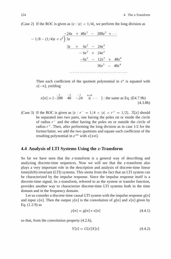
224 4 The z-Transform
(Case 2) If the ROC is given as {z : |z| < 1/4}, we perform the long division as
−24z + 48z2 − 288z3 + · · ·− 1/8 − (1/4)z + z2
)3z
3z + 6z2 − 24z3
− 6z2 + 24z3
−6z2 − 12z3 + 48z4
36z3 − 48z4
. . . . . . . . . . . . . . . . . . . . . . . . . . . . . . . . . .
Then each coefficient of the quotient polynomial in zn is equated withx[−n], yielding
x[n] = [−3
−288−248
−1−24
n=00 · · · ] : the same as Eq. (E4.7.9b)
(4.3.8b)
(Case 3) If the ROC is given as {z : r− = 1/4 < |z| < r+ = 1/2}, X[z] shouldbe separated into two parts, one having the poles on or inside the circleof radius r− and the other having the poles on or outside the circle ofradius r+. Then, after performing the long division as in case 1/2 for theformer/latter, we add the two quotients and equate each coefficient of theresulting polynomial in z±n with x[∓n].
4.4 Analysis of LTI Systems Using the z-Transform
So far we have seen that the z-transform is a general way of describing andanalyzing discrete-time sequences. Now we will see that the z-transform alsoplays a very important role in the description and analysis of discrete-time lineartime(shift)-invariant (LTI) systems. This stems from the fact that an LTI system canbe characterized by the impulse response. Since the impulse response itself is adiscrete-time signal, its z-transform, referred to as the system or transfer function,provides another way to characterize discrete-time LTI systems both in the timedomain and in the frequency domain.
Let us consider a discrete-time causal LTI system with the impulse response g[n]and input x[n]. Then the output y[n] is the convolution of g[n] and x[n] given byEq. (1.2.9) as
y[n] = g[n] ∗ x[n] (4.4.1)
so that, from the convolution property (4.2.6),
Y [z] = G[z]X [z] (4.4.2)

4.4 Analysis of LTI Systems Using the z-Transform 225
where X [z], Y [z], and G[z] are the z-transforms of the input x[n], output y[n], andimpulse response g[n], respectively. Note that G[z] is referred to as the system ortransfer function.
Remark 4.5 System Function, Pole Location, ROC, Causality, and Stability
(1) Eqs. (4.4.2) and (3.2.8) have an interpretation of describing the input-outputrelationship of a discrete-time LTI system in the z-domain and in the frequencydomain, respectively. Comparing these two equations, we can state that the sys-tem function G[z], evaluated on the unit circle z = e jΩ, yields the frequencyresponse G[e jΩ] = G(Ω) of the system (Remark 4.2) if G(Ω) = F{g[n]}exists, or equivalently, the ROC of G[z] includes the unit circle. This is anal-ogous to the continuous-time case where the frequency response G(ω) can beobtained by evaluating the system function G(s) on the imaginary axis s = jω.
(2) Characteristics of a system such as stability and causality can be associated withthe ROC and pole location of the system function G[z]. For example, if a systemis causal, its impulse response g[n] is a right-sided sequence and therefore,the ROC of G[z] = Z{g[n]} must be the outside of the outermost pole (seeRemark 4.4). If a system is stable, the ROC of G[z] includes the unit circleso that the frequency response G[e jΩ] can be defined (see Remark 4.2). If asystem is both causal and stable, then the ROC of G[z] must include the unitcircle and be outside the outermost pole. It is implied that for a causal system tobe stable, all the poles of its system function G[z] must be inside the unit circle(Fig. 4.4(a) vs. (b)).
In particular, for systems characterized by linear constant-coefficient differenceequations, the z-transform provides a very convenient procedure for obtainingthe system function, frequency response, or time response. Consider a causal lin-ear time-invariant (LTI) system (in Fig. 4.5) whose input-output relationship isdescribed by the following difference equation
∑N A−1
i=0ai y[n − i] =
∑N B−1
j=0b j x[n − j] (4.4.3)
z-planeIm{z} Im{z}
(a) All poles inside the unit circle (b) Not all poles inside the unit circle
Re{z} Re{z}1
51
4
z-plane
Fig. 4.4 Pole locations, ROC, unit circle, causality, and stability

226 4 The z-Transform
Input Output
Output spectrum
∑NA–1i=0 aiy [n– i ]
A [z ]Y [z ] = B [z ]X [z ]
bjx [n–j ]
B [z ]X [z ]
Y(Ω) B(Ω)X(Ω) A(Ω)
A [z ]Y [z ]
∑NB–1j=0
y [n ] = g [n ] * x [n ]
z-Transorm of output
Y (Ω) = G (Ω) X(Ω)
Y [z ] = G [z ]X [z ]
Input spectrumFrequency response G (Ω) =
System or transfer function G [z ] =
Impulse response g [n]x [n ]
X [z ]
X [Ω]
z-Transform of input
=
=
=
Fig. 4.5 The input–output relationship, system function, and frequency response of a discrete–timeLTI system
where the initial conditions are given as y[n0], y[n0 − 1], · · · , y[n0 − N A + 2].This can be solved iteratively for the time response y[n] to an input x[n] startingfrom n = n0 + 1:
y[n] = 1
a0
(−a1 y[n − 1] − · · · − aN A−1 y[n − N A + 1] +
∑N B−1
j=0b j x[n − j]
)(4.4.4)
With zero initial conditions and the unit impulse input x[n] = δ[n], this yieldsthe impulse response y[n] = g[n]. To find the system function as the z-domaininput-output relationship, we assume zero initial conditions and use the linearityand time-shifting properties to take the z-transform of Eq. (4.4.3) as
∑N A−1
i=0ai z
−i Y [z] =∑N B−1
j=0b j z
− j X [z]; A[z]Y [z] = B[z]X [z];
G[z] = Y [z]
X [z]= B[z]
A[z]with A[z] =
∑N A−1
i=0ai z
−i and B[z] =∑N B−1
j=0b j z
− j
(4.4.5)
This is referred to as the system function. Substituting z = e jΩ into the systemfunction or taking the DTFT of the impulse response g[n], we can obtain the fre-quency response of the system. Figure 4.6 shows the overall relationship amongthe time-domain relationship (in the form of difference equation), the system (ortransfer) function, the impulse response, and the frequency response.
∑NA–1 ∑i = 0 j = 0aiy [n–i ] =z-Transform
z -domain Frequency domain
DTFT (discrete-time Fourier transform)
Y [z ]A [z ] z = e jΩ
B [z ]G [e jΩ] G (Ω)
X [z ]G [z ]
A [z ]Y [z ] = B [z ]X [z ]Inverse z-transform
Inverse z-transform
z-Transform
zero initial conditions
Time domain
x [n] = δ[n] andg [n ]
bj x [n– j ]
== =
NB–1
Fig. 4.6 The relationship between the impulse response, system function, and frequency response

4.4 Analysis of LTI Systems Using the z-Transform 227
Especially when we are interested only in right-sided sequences and causal lin-ear systems, it is sensible to use the unilateral z-transform instead of the bilateralz-transform. It is the time shifting property that makes the unilateral z-transformparticularly useful in analyzing causal systems described by difference equationswith initial conditions.
Example 4.9 Difference Equation, System Function, and Impulse ResponseConsider a discrete-time causal LTI (linear time-invariant) system whose input-
output relationship is described by the following difference equation:
y[n] − 1
4y[n − 1] − 1
8y[n − 2] = x[n − 1] (E4.9.1)
(a) Find the system function G[z].Applying the linearity and time-shifting properties of the z-transform or usingEq. (4.4.5), we can obtain the system function as
G[z] = Y [z]
X [z]= z−1
1 − (1/4)z−1 − (1/8)z−2= z
(z − 1/2)(z + 1/4)(E4.9.2)
(b) Find the impulse response g[n].Noting that the system is causal and accordingly, the ROC of G[z] is z > 1/2(the outside of the circle passing through the outermost pole), we obtain theinverse z-transform of G[z] as
g[n] = Z−1
{z
(z − 1/2)(z + 1/4)
}partial fraction expansion=
Z−1
{4
3
(z
z − 1/2− z
z + 1/4
)}B.9(5)= 4
3
((1
2
)n
−(
−1
4
)n)us[n]
(E4.9.3)
Alternatively, the impulse response can be obtained directly from the dif-ference equation, which can be solved iteratively with the unit impulse inputx[n] = δ[n] and zero initial conditions:
y[n] = 1
4y[n − 1] + 1
8y[n − 2] + x[n − 1] (E4.9.4)
where y[−1] = y[−2] = 0 and x[n − 1] = δ[n − 1] = 1 only for n = 1.
n = 0 : y[0] = (1/4)y[−1] + (1/8)y[−2] + x[−1] = 0 − 0 + 0 = 0
n = 1 : y[1] = (1/4)y[0] + (1/8)y[−1] + x[0] = 0 − 0 + 1 = 1
n = 2 : y[2] = (1/4)y[1] + (1/8)y[0] + x[1] = 1/4 − 0 + 0 = 1/4
n = 3 : y[3] = (1/4)y[2] + (1/8)y[1] + x[2] = 1/16 + 1/8 + 0 = 3/16
. . . . . . . . . . . . . . . . . . ..

228 4 The z-Transform
%sig04e09.msyms z, Gz=z/(zˆ2-(1/4)*z-1/8); %system functiong = iztrans(Gz) % symbolic inverse z transformN=16; nn=[0:N-1];for n=0:N-1, gn(n+1) = eval(g); end% Solving the difference equation with the unit impulse inputB= [1 0]; A= [1 -1/4 -1/8]; %numerator/denominatorNB=length(B); NA=length(A);xn = [0 1 zeros(1,N-1+NB)]; % x[n-1] impulse input delayed by one sampley = zeros(1,NA-1); % Initial conditionfor m=NA:NA+N-1 % To solve the difference equation iteratively
y(m)= -A(2:NA)*y(m-[1:NA-1]).’ +B*xn(m-NA+[1:NB]).’;endy = y(NA:NA+N-1);% Using filter()yp=[0 0]; xp=0; w0=filtic(B,A,yp,xp) %Initial condition from past historyyn = filter(B,A,xn,w0) % With zero initial condition by defaultsubplot(211)stem(nn,gn), hold on, pause, stem(nn,y(1:N),’r’), stem(nn,yn(1:N),’k.’)% To plot the frequency responseN=64; dW=2*pi/N; W=[0:N]*dW; % frequency rangeGW = DTFT(gn,W); %DTFT of the impulse responseGW1 = freqz(B,A,W); %substitute z=exp(j*W) into the system ftn B(z)/A(z)subplot(212), plot(W,abs(GW),’b’, W,abs(GW1),’r’)
The objective of the above program “sig04e09.m” is as follows:
- Find the impulse response g[n] in two ways, that is, by taking the inverse z-transform of the system function G[z] and by solving the difference equation forthe output y[n] to the impulse input x[n] = δ[n]. The MATLAB built-in function‘filter()’ together with ‘filtic()’ (Sect. E.12) can also be used to obtainthe output to any input and any initial condition. Also check if the two resultsconform to each other.
- Find the frequency response G(Ω) in two ways, that is, by taking the DTFT ofthe impulse response g[n] and by substituting z = e jΩ into the system functionG[z] = B[z]/A[z], where the latter job is done by using the MATLAB built-infunction ‘freqz()’.
(cf) Comparing Eq. (E4.9.2) with Eq. (E4.9.3), we can tell that the poles of thesystem function, say, p1 = 1/2 and p2 = −1/4 yield the modes of the sys-tem, each of which determines how the corresponding output term evolves withtime. See the stability theorem A.1.
Remark 4.6 Computational Method for Inverse z-TransformExample 4.9 suggests another way of obtaining the inverse z-transform. That
is, we can regard a rational z-transform expression G[z] as a system function andset it equal to Y [z]/X [z]. Then, cross multiplying yields the z-domain input-outputrelationship
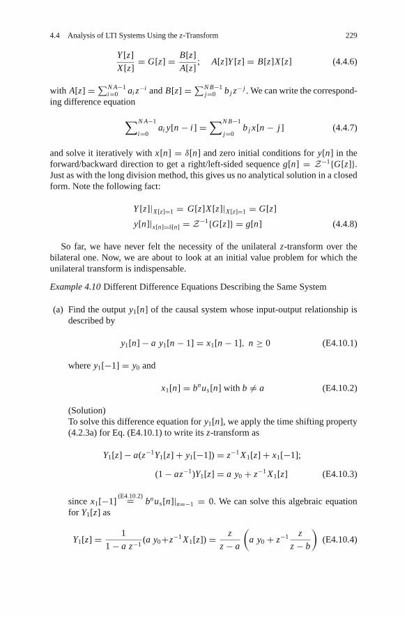
4.4 Analysis of LTI Systems Using the z-Transform 229
Y [z]
X [z]= G[z] = B[z]
A[z]; A[z]Y [z] = B[z]X [z] (4.4.6)
with A[z] = ∑N A−1i=0 ai z−i and B[z] = ∑N B−1
j=0 b j z− j . We can write the correspond-ing difference equation
∑N A−1
i=0ai y[n − i] =
∑N B−1
j=0b j x[n − j] (4.4.7)
and solve it iteratively with x[n] = δ[n] and zero initial conditions for y[n] in theforward/backward direction to get a right/left-sided sequence g[n] = Z−1{G[z]}.Just as with the long division method, this gives us no analytical solution in a closedform. Note the following fact:
Y [z]|X [z]=1 = G[z]X [z]|X [z]=1 = G[z]
y[n]|x[n]=δ[n] = Z−1{G[z]} = g[n] (4.4.8)
So far, we have never felt the necessity of the unilateral z-transform over thebilateral one. Now, we are about to look at an initial value problem for which theunilateral transform is indispensable.
Example 4.10 Different Difference Equations Describing the Same System
(a) Find the output y1[n] of the causal system whose input-output relationship isdescribed by
y1[n] − a y1[n − 1] = x1[n − 1], n ≥ 0 (E4.10.1)
where y1[−1] = y0 and
x1[n] = bnus[n] with b �= a (E4.10.2)
(Solution)To solve this difference equation for y1[n], we apply the time shifting property(4.2.3a) for Eq. (E4.10.1) to write its z-transform as
Y1[z] − a(z−1Y1[z] + y1[−1]) = z−1 X1[z] + x1[−1];
(1 − az−1)Y1[z] = a y0 + z−1 X1[z] (E4.10.3)
since x1[−1](E4.10.2)= bnus[n]|n=−1 = 0. We can solve this algebraic equation
for Y1[z] as
Y1[z] = 1
1 − a z−1(a y0+z−1 X1[z]) = z
z − a
(a y0 + z−1 z
z − b
)(E4.10.4)

230 4 The z-Transform
To take the inverse z-transform of this expression, we divide its both sides byz and perform the partial fraction expansion as
Y1[z]
z= a y0
z − a+ 1
(z − a)(z − b)= a y0
z − a+ 1
a − b
(1
z − a− 1
z − b
)
Y1[z] = a y0z
z − a+ 1
a − b
(z
z − a− z
z − b
)(E4.10.5)
Now we take the inverse z-transform to get the output as
y1[n] = ay0anus[n] + 1
a − b(an − bn)us[n]
= y0an+1us[n + 1] + 1
a − b(an − bn)us[n] (E4.10.6)
Here, we replaced us[n] by us[n+1] to express the existence of the given initialcondition y1[−1] = y0.
(b) Find the output y2[n] of the causal system whose input-output relationship isdescribed by
y2[n + 1] − ay2[n] = x2[n], n ≥ 0 (E4.10.7)
where y2[0] = y0 and
x2[n] = x1[n − 1] = bn−1us[n − 1] with b �= a (E4.10.8)
(Solution)To solve this difference equation for y2[n], we apply the time shifting property(4.2.3b,a) for Eq. (E4.10.7) to write its z-transform as
z(Y2[z] − y2[0]) − aY2[z] = X2[z];
(z − a)Y2[z] = zy0 + X2[z] = zy0 + z−1 X1[z] (E4.10.9)
since x1[−1](E4.10.2)= bnus[n]|n=−1 = 0. We can solve this algebraic equation
for Y2[z] as
Y2[z] = 1
z − a(zy0 + z−1 X1[z]) = y0z
z − a+ 1
(z − a)(z − b)(E4.10.10)
To take the inverse z-transform of this expression, we divide its both sides byz and perform the partial fraction expansion as
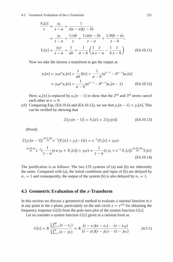
4.5 Geometric Evaluation of the z-Transform 231
Y2[z]
z= y0
z − a+ 1
z(z − a)(z − b)
= y0
z − a+ 1/ab
z+ 1/a(a − b)
z − a+ 1/b(b − a)
z − b;
Y2[z] = y0z
z − a+ 1
ab+ 1
a − b
(1
a
z
z − a− 1
b
z
z − b
)(E4.10.11)
Now we take the inverse z-transform to get the output as
y2[n] = y0anus[n] + 1
abδ[n] + 1
a − b(an−1 − bn−1)us[n]
= y0anus[n] + 1
a − b(an−1 − bn−1)us[n − 1] (E4.10.12)
Here, us[n] is replaced by us[n − 1] to show that the 2nd and 3rd terms canceleach other at n = 0.
(cf) Comparing Eqs. (E4.10.6) and (E4.10.12), we see that y1[n − 1] = y2[n]. Thiscan be verified by showing that
Z{y1[n − 1]} = Y2[z] = Z{y2[n]} (E4.10.13)
(Proof)
Z{y1[n − 1]} (4.2.3a)= z−1(Y1[z] + y1[−1]z) = z−1(Y1[z] + y0z)
(4.10.4)= z−1(1
z − a(z a y0 + X1[z]) + y0z) = 1
z − a(z y0 + z−1 X1[z])
(4.10.10)= Y2[z]
(E4.10.14)
The justification is as follows: The two LTI systems of (a) and (b) are inherentlythe same. Compared with (a), the initial conditions and input of (b) are delayed byn1 = 1 and consequently, the output of the system (b) is also delayed by n1 = 1.
4.5 Geometric Evaluation of the z-Transform
In this section we discuss a geometrical method to evaluate a rational function in zat any point in the z-plane, particularly on the unit circle z = e jΩ for obtaining thefrequency response G(Ω) from the pole-zero plot of the system function G[z].
Let us consider a system function G[z] given in a rational form as
G[z] = K
∐Mj=1 (z − z j )∐Ni=1 (z − pi )
= K(z − z1)(z − z2) · · · (z − zM )
(z − p1)(z − p2) · · · (z − pN )(4.5.1)

232 4 The z-Transform
where z j ’s and pi ’s are finite zeros and poles of G[z], respectively. The value ofG[z] at some point z = z0 in the z-plane is a complex number that can be expressedin the polar form as
G[z0] = |G[z0]|∠G[z0] (4.5.2)
where
Magnitude : |G[z0]| = |K |∐M
j=1 |z0 − z j |∐Ni=1 |z0 − pi |
(4.5.3a)
Phase : ∠G[z0] =∑M
j=1∠(z0 − z j ) −
∑N
i=1∠(z0 − pi )(±π)
with ± π only for K < 0 (4.5.3b)
(z0 − z j )’s and (z0 − pi )’s in the above equations are complex numbers, each ofwhich can be represented by a vector in the z-plane from z j or pi to z0. They canbe easily constructed from the pole/zero plot where |z0 − z j | and |z0 − pi | are thedistances, while ∠z0 − z j and ∠z0 − pi are the phase angles.
As mentioned in Remark 4.5(1), the frequency response G(Ω) can be obtainedby evaluating the system function G[z] on the unit circle if it exists. Keeping this inmind, we can use the pole-zero plot to get the approximate shape of the magnituderesponse |G(Ω)| without computing the frequency response from Eq. (4.5.2). Hereis the overall feature of frequency response related with the pole-zero pattern:
Remark 4.7 Frequency (Magnitude/Phase) Response and Pole-Zero Pattern
(1) For a pole/zero near the unit circle, the magnitude response curve tends to havea sharp peak/valley and the phase changes rapidly by about 180◦ at the corre-sponding frequency. As the pole/zero moves to the unit circle, the peak/valleybecomes sharper. On the other hand, as the pole/zero moves to the origin, thepeak/valley becomes smoother. Such a tendency can be observed from Fig. 3.2where the frequency responses of G[z] = z/(z−a) are depicted for a = 0.8 and0.5. Also, the phase jump of π [rad] occurring at the frequency correspondingto a zero on the unit circle is illustrated by Figs. 3.1, 3.7, 3.11, and 4.8.
(2) Generally speaking, if a singularity (pole/zero) is located close to the unit circle,it will dominate the frequency response in the frequency range adjacent to thatlocation. This idea of dominant singularity is helpful not only for getting anapproximate frequency response, but also for the pole/zero placement designto achieve a desired frequency response. For example, the magnitude response(Fig. 4.7(b)) of the system described by (E4.11.1) has the maximum aroundΩ = ±π/4 due to the pole at z = 0.5
√2e± jπ/4 and becomes zero at Ω = π
because of the zero at z = −1. In contrast, the zero at z = 0 (which is far fromthe unit circle) has no influence on the magnitude response.

4.5 Geometric Evaluation of the z-Transform 233
Example 4.11 Pole-Zero Pattern and Frequency ResponseFor the system function
G[z] = z(z + 1)
z2 − z + 0.5= z(z + 1)
(z − 0.5 − j0.5)(z − 0.5 + j0.5)(E4.11.1)
we have the pole-zero plot and the frequency response magnitude and phase curvesdepicted in Fig. 4.7(a), (b), and (c), respectively. As shown in Fig. 4.7(b), the mag-nitude of G(Ω) = G[e jΩ] becomes zero at Ω = π corresponding to the zeroz = −1, i.e.,
|G[e jΩ]|∣∣Ω=π
= |G[z]||z=−1 = 0 (E4.11.2)
Im {z}
[rad]
Re {z}
AB
G [z ]
CD
z0 = e j Ω
B
(a) The pole–zero plot of G [z] =
(b) The magnitude curve of the frequency response G(Ω) = G [e j Ω]
(c) The phase curve of the frequency response G(Ω) = G [e j Ω]
z
2–z+0.5
z 2–z+0.5
Z1Z 2
P2
P1
z (z+1)
z (z+1)(z –0.5– j 0.5) (z –0.5+ j 0.5)
z (z+1)
C
D
A
Ω = −πΩ = π Ω = 0
Ω = 2π
Ω = −π/4
2π
2π
π
φ1
φ2
θ1
<(θ1 + θ2 − φ1 − φ2 )
θ2
−π
−π
|G [e j Ω]
G [e j Ω]
Ω
Ω
ΩP = 0.68
Ω = π/4
G[z0] =
0
2
2
– 0.7457
–2
5.3
π
4
0
=
=
1
Fig. 4.7 The pole–zero plot and frequency response for Example 4.11

234 4 The z-Transform
and it reaches the peak around Ω = ±π/4 adjacent to the phases of the poles
z = 0.5 ± j0.5 = 0.5√
2e± jπ/4 (E4.11.3)
(a) Let us find the response of the system G[z] to a sinusoidal input x1[n] =sin(Ωpn) with Ωp = 0.68.
Y1[z] = X1[z]G[z] = z sin Ωp
(z − cos Ωp)2 + sin2 Ωp
z(z + 1)
(z − 0.5)2 + 0.52(E4.11.4)
= −3.60 × z(z − cos Ωp) + 3.89 × z sin Ωp
(z − cos Ωp)2 + sin2 Ωp
+ 3.60 × z(z − R cos Ωs) − 1.65 × z R sin Ωs
(z − R cos Ωs)2 + (R sin Ωs)2
∣∣∣∣R= 1√
2,Ωs= π
4
y1[n] = Z−1 {Y1[z]} = −3.6 cos(Ωpn) + 3.89 sin(Ωpn)
+√
2−n
(3.6 cos(nπ/4) − 1.65 sin(nπ/4))
= (5.3 sin(Ωpn − 0.7457) +√
2−n
(3.6 cos(nπ/4)
− 1.65 sin(nπ/4)))us[n] (E4.11.5)
Note that the sinusoidal steady-state response y1,ss[n] = 5.3 sin(Ωpn − 0.7457)has the same frequency with the input x1[n], but its amplitude is |G(Ωp)| = 5.3times that of the input and its phase is ∠G(Ωp) = −0.7457 � −1.1Ωp plusthat of the input, as can be seen from Fig. 4.8(a).
(b) Let us find the response of the system G[z] to a unit step (DC) input x2[n] =us[n].
4
0
0
0
05
20
20
30
30
n
m
(b) The output of the system of Example 4.11 to a unit step (DC) input
(a) The output of the system of Example 4.11 to a sinusoidal input sin (Ωpn)
10
11
–5.3
OutputInput
5.3
::
Fig. 4.8 The output of the system of Example 4.11 to sinusoidal/DC inputs

4.5 Geometric Evaluation of the z-Transform 235
Y2[z] = X2[z]G[z] = z
z − 1
z(z + 1)
(z − 0.5)2 + 0.52
= 4 × z
z − 1+ −3 × z(z − 0.5)
(z − 0.5)2 + 0.52+ 1 × z0.5
(z − 0.5)2 + 0.52(E4.11.6)
where the partial fraction expansion is found as follows:
Y2[z] = K1 × z
z − 1+ K2 × z(z − 0.5)
(z − 0.5)2 + 0.52+ K3 × z0.5
(z − 0.5)2 + 0.52
K1 = (z − 1)Y1[z]
z= z(z + 1)
(z − 0.5)2 + 0.52
∣∣∣∣z=1
= 4
K1 + K2 = 1,−K1 − 0.5K2 + 0.5K3 = 1, 0.5K1 + 0.5K2 − 0.5K3 = 0
K2 = 1 − K1 = 1 − 4 = −3, K3 = K1 + K2 = 4 − 3 = 1
Thus the response to x2[n] = us[n] can be obtained from the inverse z-transform as
y2[n] = Z−1 {Y2[z]} =(
4 +√
2−n
(−3 cos(nπ/4) + sin(nπ/4)))
us[n]
(E4.11.7)
Note that the DC steady-state response y2,ss[n] = 4 is the DC gain |G(0)| = 4times that of the input, as can be seen from Fig. 4.8(b).
In fact, the inverse z-transform of Y1[z] as well as Figs. 4.7 and 4.8 is obtainedby running the following MATLAB program “sig04e11.m”, where we managed toget the coefficients of the partial fraction expansion using residue() since iztrans()does not work properly for this case.
%sig04e11.mclear, clfB=[1 1 0]; A=[1 -1 0.5]; %numerator/denominator of system function (E4.11.1)figure(1), zplane(roots(B),roots(A)) % pole-zero plot in Fig. 4.7(a)% To get the frequency responseN=360; dW=2*pi/N; k0=-200; W=[k0:500]*dW;GW= freqz(B,A,W); % frequency responseGW mag= abs(GW); GW ph= angle(GW); % magnitude/phase of frequency response[GW mag peak,i]= max(GW mag(-k0+[1:N/2])) % peak frequency response magnitudeip=-k0+i-1; Wp=W(ip); GW ph peak=GW ph(ip); % peak frequencyGW dc= GW(-k0+1); % DC gainfigure(2), subplot(411), plot(W,GW mag) % Fig. 4.7(b)subplot(412), plot(W,GW ph) % Fig. 4.7(c)% To get the time response from filtering of a sine-wave input signalnn=[0:30]; % time index vectorxn= sin(Wp*nn); % A sinusoidal input of peak frequencyyn= filter(B,A,xn); % With zero initial condition by default% plot the time responsesubplot(413), stem(nn,xn,’Markersize’,5), hold on

236 4 The z-Transform
stem(nn,yn,’x’,’Markersize’,5)% Try with the inverse z-transformsyms zy1=iztrans(sin(Wp)*zˆ2*(z+1)/((z-cos(Wp))ˆ2+sin(Wp)ˆ2)/((z-0.5)ˆ2+0.5ˆ2))[r,p,k]=residue(sin(Wp)*[1 1 0],conv([1 -2*cos(Wp) 1],[1 -1 0.5]))R = sqrt(real(p(3)*p(4))); Ws= angle(p(3));% numerator of the 1st&2nd terms reduced to a common denominatorn1= r(1)*[1 -p(2)]+r(2)*[1 -p(1)];K1= n1(1); K2= (n1(2)+K1*cos(Wp))/sin(Wp);% numerator of the 3rd&4th terms reduced to a common denominatorn2= r(3)*[1 -p(4)]+r(4)*[1 -p(3)];K3= n2(1); K4= (n2(2)+K3*R*cos(Ws))/(R*sin(Ws));y1n= K1*cos(Wp*nn) + K2*sin(Wp*nn) + R.ˆnn.*(K3*cos(Ws*nn)+K4*sin(Ws*nn));stem(nn,y1n,’rx’,’Markersize’,5)%filtering of a DC input signalnn=[0:30]; xn= ones(size(nn)); % A DC input signal (of zero frequency)yn DC= filter(B,A,xn); % With zero initial condition by defaultsubplot(414)stem(nn,xn,’Markersize’,5) % plot the time response together with the inputhold on, stem(nn,yn DC,’m’,’Markersize’,5)% Try with the inverse z-transformy2=iztrans(zˆ2*(z+1)/(z-1)/((z-0.5)ˆ2+0.5ˆ2))% A nice alternative for the case of all simple poles[r,p,k]=residue([1 1 0],conv([1 -1],[1 -1 0.5]))y2n= 0;for i=1:length(r)
y2n= y2n + r(i)*p(i).ˆnn;endstem(nn,real(y2n),’mˆ’,’Markersize’,5)
4.6 The z-Transform of Symmetric Sequences
In this section we explore some features of the phase characteristic and pole-zeropattern for systems having (anti-)symmetric impulse responses of finite duration.
4.6.1 Symmetric Sequences
Let us consider a symmetric sequence g[n] of duration N + 1 such that
g[n] = g[N − n] for n = 0 : N (4.6.1)
<Case 1> If N is even, i.e., N = 2M for some integer M , then the z-transform ofg[n] is
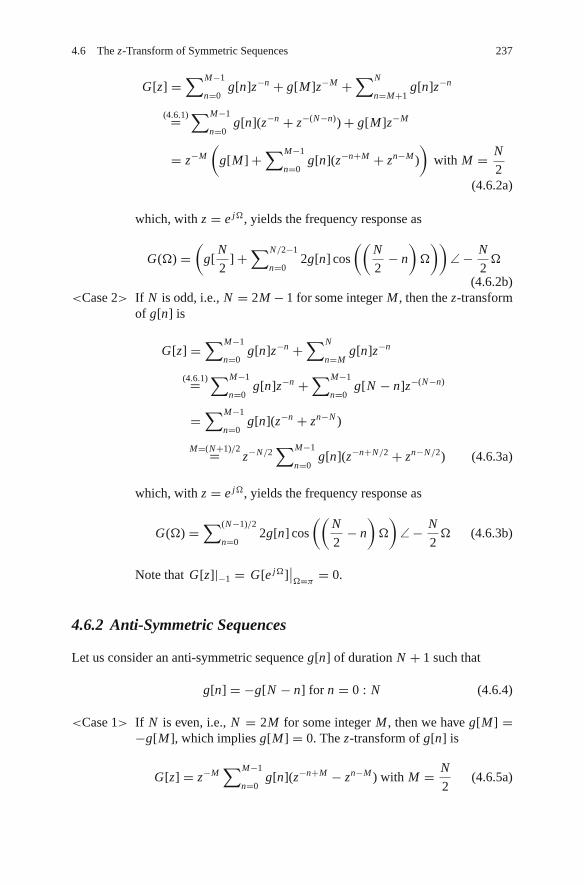
4.6 The z-Transform of Symmetric Sequences 237
G[z] =∑M−1
n=0g[n]z−n + g[M]z−M +
∑N
n=M+1g[n]z−n
(4.6.1)=∑M−1
n=0g[n](z−n + z−(N−n)) + g[M]z−M
= z−M
(g[M] +
∑M−1
n=0g[n](z−n+M + zn−M )
)with M = N
2(4.6.2a)
which, with z = e jΩ, yields the frequency response as
G(Ω) =(
g[N
2] +
∑N/2−1
n=02g[n] cos
((N
2− n
)Ω
))∠ − N
2Ω
(4.6.2b)<Case 2> If N is odd, i.e., N = 2M − 1 for some integer M , then the z-transform
of g[n] is
G[z] =∑M−1
n=0g[n]z−n +
∑N
n=Mg[n]z−n
(4.6.1)=∑M−1
n=0g[n]z−n +
∑M−1
n=0g[N − n]z−(N−n)
=∑M−1
n=0g[n](z−n + zn−N )
M=(N+1)/2= z−N/2∑M−1
n=0g[n](z−n+N/2 + zn−N/2) (4.6.3a)
which, with z = e jΩ, yields the frequency response as
G(Ω) =∑(N−1)/2
n=02g[n] cos
((N
2− n
)Ω
)∠ − N
2Ω (4.6.3b)
Note that G[z]|−1 = G[e jΩ]∣∣Ω=π
= 0.
4.6.2 Anti-Symmetric Sequences
Let us consider an anti-symmetric sequence g[n] of duration N + 1 such that
g[n] = −g[N − n] for n = 0 : N (4.6.4)
<Case 1> If N is even, i.e., N = 2M for some integer M , then we have g[M] =−g[M], which implies g[M] = 0. The z-transform of g[n] is
G[z] = z−M∑M−1
n=0g[n](z−n+M − zn−M ) with M = N
2(4.6.5a)

238 4 The z-Transform
which, with z = e jΩ, yields the frequency response as
G(Ω) =∑N/2−1
n=02g[n] sin
((N
2− n
)Ω
)∠ − N
2Ω + π
2(4.6.5b)
Note that G[e jΩ]∣∣Ω=0 = 0 and G[e jΩ]
∣∣Ω=π
= 0.<Case 2> If N is odd, i.e., N = 2M − 1 for some integer M , then the z-transform
of g[n] is
G[z] = z−N/2∑M−1
n=0g[n](z−n+N/2 − zn−N/2) (4.6.6a)
which, with z = e jΩ, yields the frequency response as
G(Ω) =∑(N−1)/2
n=02g[n] sin
((N
2− n
)Ω
)∠ − N
2Ω + π
2(4.6.6b)
Note that G[e jΩ]∣∣Ω=0 = 0.
Remark 4.8 Pole-Zero Pattern and Linear Phase of (Anti-)Symmetric Sequences
(1) From Eqs. (4.6.2a)/(4.6.5a) and (4.6.3a)/(4.6.6a), we can see that if G[z0] = 0,then G[z−1
0 ] = 0, which implies that real zeros occur in reciprocal pairs (z0
and z−10 ) and complex zeros occur in reciprocal, complex-conjugate quadruplets
(z0 = r0∠ ± Ω0 and z−10 = r−1
0 ∠ ± Ω0). Note that zeros on the unit circle formtheir own reciprocal pairs and real zeros on the unit circle, i.e., z = 1 or z = −1,form their own reciprocal, complex conjugate pairs. Note also that all the polesare located at z = 0 or ∞. See Fig. 4.9(a1) and (a2).
(2) From Eqs. (4.6.2b)/(4.6.5b) and (4.6.3b)/(4.6.6b), we can see that they havelinear phase, i.e., their phases are (piecewise) linear in Ω except for phase jumpsof ±π or ±2π (see Remark 3.3 and Fig. 4.9(c1) and (c2)).
(3) If a system has the impulse response represented by a symmetric or anti-symmetric sequence of finite duration, such a system has linear phase shiftingproperty so that it will reproduce the input signals falling in the passband with adelay equal to the slope of the phase curve. That is why such a system is calledthe linear phase FIR filter.
Example 4.12 Pole-zero Pattern of Symmetric or Anti-symmetric Sequences
(a) Consider a system whose impulse response is
g1[n] = [· · · n=−10
01
1−2.5
25.25
3−2.5
41.0
50 · · · ]. (E4.12.1)
This system has the system function G1[z] = Z{g1[n]} as
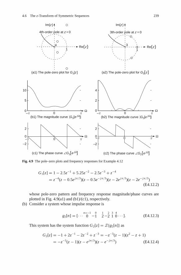
4.6 The z-Transform of Symmetric Sequences 239
π(b1) The magnitude curve G1[e jΩ]
(a1) The pole-zero plot for G1[z ] (a2) The pole-zero plot for G2[z]
Im{z} Im{z}
41
0
0 0
–π
–π
π
π π
0–πΩ
Ω Ω
Ω0
–2
0
2
–2
0
2
5
10 4
2
0
3Re{z} Re{z}
(c1) The phase curve ∠G1[e jΩ] (c2) The phase curve ∠G2 [e jΩ]
(b2) The magnitude curve G2[e jΩ]
4th-order pole at z = 0 3th-order pole at z = 0
1
–π
Fig. 4.9 The pole–zero plots and frequency responses for Example 4.12
G1[z] = 1 − 2.5z−1 + 5.25z−2 − 2.5z−3 + z−4
= z−4(z − 0.5e jπ/3)(z − 0.5e− jπ/3)(z − 2e jπ/3)(z − 2e− jπ/3)(E4.12.2)
whose pole-zero pattern and frequency response magnitude/phase curves areplotted in Fig. 4.9(a1) and (b1)/(c1), respectively.
(b) Consider a system whose impulse response is
g2[n] = [· · · n=−10 −0
112 −2
231
40 · · · ]. (E4.12.3)
This system has the system function G2[z] = Z{g2[n]} as
G2[z] = −1 + 2z−1 − 2z−2 + z−3 = −z−3(z − 1)(z2 − z + 1)
= −z−3(z − 1)(z − e jπ/3)(z − e− jπ/3) (E4.12.4)

240 4 The z-Transform
whose pole-zero pattern and frequency response magnitude/phase curves areplotted in Fig. 4.9(a2) and (b2)/(c2), respectively.
The following program “sig04e12.m” is run to yield Fig. 4.9, where zplane(B,A)is used to create the pole-zero plot of a system with system function G[z] =B[z]/A[z].
%sig04e12.mclear, clfN=360; W=pi/N*[-N:N]; % frequency rangefor i=1:2
if i==1, B=[1 -2.5 5.25 -2.5 1]; A=1;else B=[-1 2 -2 1]; A=1; %numerator/denominator of system functionendfigure(1), subplot(220+i), zplane(B,A)GW= freqz(B,A,W); % frequency responseGW mag= abs(GW); % magnitude of frequency responseGW phase= angle(GW); % phase of frequency responsefigure(2)subplot(220+i), plot(W,GW mag)set(gca,’fontsize’,9, ’Xlim’,[-pi pi], ’xtick’,[-pi 0 pi], ...
’xticklabel’,{’-pi’ ’0’ ’pi’})subplot(222+i), plot(W,GW phase)set(gca,’fontsize’,9, ’Xlim’,[-pi pi], ’xtick’,[-pi 0 pi], ...
’xticklabel’,{’-pi’ ’0’ ’pi’})end
4.7 Summary
In this chapter we have defined the bilateral/unilateral z-transform and derived theirbasic properties. We have also presented the several methods to find the inversez-transform of a given z-transform expression. We have explored the relation-ship among the system function, frequency response, and difference equation anddiscussed how to utilize the z-transform for analyzing discrete-time LTI systems.
Problems
4.1 z-Transform
(a) Find the bilateral z-transform X [z] (with its ROC) of
x[n] = a|n| = anus[n] + a−nus[−n − 1] with |a| < 1 (P4.1.1)
(b) Could you get the bilateral z-transform of
x[n] = 1 = us[n] + us[−n − 1] (P4.1.2)
If your answer is yes, find it. Otherwise, state why it is not possible.

Problems 241
(c) Find the bilateral z-transform X [z] (with its ROC) of
x[n] = us[−n] (P4.1.3)
in the following three ways:
(i) Noting that us[−n] is the one-sample delayed version of us[−n − 1],use the time shifting property.
(ii) Noting that us[−n] is the time-reversal version of us[n], use the timereversal property.
(iii) Noting that us[−n] can be expressed as us[−n − 1] + δ[n], use B.9(6)& (1).
4.2 Inverse z-Transform
(a) Find the inverse z-transform x[n] of
X [z] = z2
(z + 1)2= z × z
(z + 1)2= z
z + 1× z
z + 1(P4.2.1)
with ROC R = {z : |z| > 1}
in the following two different ways:
(i) Use the z-transform table B.9(10) and the time shifting property4.2.3(b) or B.7(2).
(ii) Use the z-transform table B.9(5) and the convolution property 4.2.6or B.7(4).
(b) Use the z-transform table B.9(17) and the time shifting property 4.2.3(a) orB.7(2) to find the inverse z-transform of
X [z] = a
z2 + a2= z−1 × az
z2 + a2with ROC R = {z : |z| > a} (P4.2.2)
(c) Find the inverse z-transform x[n] of
X [z] = 2z − 1
(z − 1)(z2 − z + 1)with ROC R = {z : |z| > 1} (P4.2.3)
(d) Find the inverse z-transform x[n] of
X [z] = 1
(z − 1)2z2= 1
(z − 1)2− 2
z − 1+ 1
z2+ 2
z(P4.2.4)
with ROC R = {z : |z| > 1}
4.3 Inverse z-Transform, Causality, Convergence, and Stability
(a) Find the inverse z-transforms ga1[n], ga2[n], and ga3[n] of
Ga[z] = 3(1 − z−1)
1 − (5/2)z−1 + z−2= 3z(z − 1)
(z − 2)(z − 1/2)(P4.3.1)

242 4 The z-Transform
with one of the following ROCs:
(i) R1 = {z : |z| > 2}, (ii) R2 = {z : |z| < 1/2}, and (iii) R3 = {z :1/2 < |z| < 2}. Then determine the causality and convergence (tozero) for each of gi [n]’s.
(b) Find the inverse z-transforms gb1[n], gb2[n], and gb3[n] of
Gb[z] = 2z(z + 1)
z2 + (3/4)z + 1/8= 2z(z + 1)
(z + 1/4)(z + 1/2)(P4.3.2)
with one of the following ROCs: (i) R1 = {z : |z| > 1/2}, (ii) R2 = {z :|z| < 1/4}, and (iii) R3 = {z : 1/4 < |z| < 1/2}. Then determine thecausality and convergence (to zero) for each of gi [n]’s.
(c) Suppose Ga[z] and Gb[z] are the system functions of discrete-time sys-tems. Then the causality and stability of the systems depends on thecausality and geometric convergence (to zero) of the impulse responsegi [n]’s. Referring to the stability criterion that the ROC should contain theunit circle (Remark 4.5(2)), determine the stability of the above six cases.For each case, plot the impulse response for n = −20 : 20 and completethe following table:
(d) What do you think about the stability of a system having a pole on the unitcircle, which is the boundary between the stability and instability regions?Let us consider a system with the system function
Gc[z] = 1
z − 1with ROC R = {z : |z| > 1} (P4.3.3)
Suppose a bounded input such as the unit step sequence x[n] = us[n] isapplied to this system and find the output. Is it bounded? Is the system(BIBO) stable? Can you find any (bounded) input such as a sine-wavewhich makes the output of the system blow up?
(cf) If a discrete-time LTI system has all its poles inside or on the unit circleand the poles on the unit circle are simple (distinct), the system is said tobe marginally stable. Likewise, if a continuous-time LTI system has all itspoles inside the LHP (left-half s -plane) or on the jω-axis and the poles
Table P4.3 Pole location, ROC, causality, and stability of a system
All poles inside the unit circle The unit circle inside ROC Causality Stablility
(a)–(i)(a)–(ii)(a)–(iii)(b)–(i)(b)–(ii)(b)–(iii)

Problems 243
on the jω-axis are simple (distinct), the system is said to be marginallystable.
4.4 To Solve Difference Equation Using the z-TransformConsider the following difference quation
y[n] − 1
3y[n − 1] = x[n] with x[n] = 2−nus[n] (P4.4.1)
(a) Solve it with the initial condition y[−1] = −3.(b) Solve it with the initial condition y[−1] = 6.
(cf) This problem implies that the output of an LTI system has generally thesystem mode (in the natural response) and the input mode (in the forcedresponse), but the system mode may disappear depending on the initialconditions.
4.5 Forward/Backward Solution of Difference Equation by IterationConsider the following difference quation:
y[n] − 1
4y[n − 1] − 1
8y[n − 2] = 3x[n − 1] with x[n] = δ[n] (P4.5.1)
(a) Solve it forward with no initial condition (y[−2] = y[−1] = 0) to findy[n] for n = 0 : 3. To do this, you should rewrite the difference equation as
y[n] = 1
4y[n − 1] + 1
8y[n − 2] + 3x[n − 1] with x[n] = δ[n] (P4.5.2)
(b) Solve it backward with no initial condition (y[1] = y[2] = 0) to find y[n]for n = −3 : 0. To do this, you should rewrite the difference equation as
y[n − 2] = −2y[n − 1] + 8y[n] − 24x[n − 1] with x[n] = δ[n] (P4.5.3)
(cf) You can use the following program “sig04p 05.m”. Do the results agreewith the solutions (4.3.8a,b) obtained using the long division in Sec. 4.3.2or (E4.7.9a,b)?
%sig04p 05.mclear% To solve a difference equation forward by iterationya(1)=0; ya(2)=0; % zero initial conditionsxa= zeros(1,10); xa(3)=1; % unit impulse inputfor n=3:11
ya(n)= (1/4)*ya(n-1) + (1/8)*ya(n-2) +3*xa(n-1);endnn=0:8; ya1= 4*(1/2).ˆnn - 4*(-1/4).ˆnn;[ya(3:end); ya1]% To solve a difference equation backward by iteration

244 4 The z-Transform
yb(10)=0; yb(11)=0; % zero initial conditionsxb= zeros(1,10); xb(9)=1; % unit impulse inputfor n=11:-1:3
yb(n-2)= -2*yb(n-1) + 8*yb(n) -24*xb(n-1);endybnn=-8:0; yb1= -4*(1/2).ˆnn + 4*(-1/4).ˆnn;[yb(1:end-2); yb1]
4.6 Difference Equation, System Function, Impulse Response, and FrequencyResponseConsider a causal system whose input-output relationship is described by thefollowing difference quation:
y[n] − y[n − 1] + 0.5y[n − 2] = x[n] + x[n − 1] with y[−2] = y[−1] = 0(P4.6.1)
(a) Find the system function G[z] = Y [z]/X [z] and determine the stabilitybased on its pole locations.
(b) Find the frequency response G(Ω) = G[e jΩ] at Ω = 0, π/2, and π ore jΩ = 1, j , and −1 where G(0) = G[e j0 = 1] is referred to as the DC(direct current) gain.
(c) Find the impulse response g[n], i.e., the output of the system to the unitimpulse input x[n] = δ[n] in two ways; once using the z-transform andonce using the iterative method for n = 0 : 4. Does the DTFT of {g[n] :n = 0 : 100} agree with G(Ω) for Ω = 0 : 0.01 : 2π? You can use thefollowing program “sig04p 06.m”.
(d) Find the step response, i.e., the output of the system to the unit step inputx[n] = us[n] in two ways; once using the z-transform and once using theiterative method for n = 0 : 4. Is the steady-state value the same as the DCgain obtained in (b) and the result of applying the final value theorem?
(e) Find the z-transform Y [z] of the output to a sinusoidal input x[n] =sin(nπ/2)us[n]. Find the steady-state response of the output by taking theinverse z-transform of Y [z] or using the frequency response obtained in (b).Support your analytical solution by plotting it together with the iterative(numerical) solution for n = 0 : 100. Could you apply the final valuetheorem? If not, state why it is not possible.
%sig04p 06.mclear, clfdisp(’(a)’)syms z% Gz= z*(z+1)/(zˆ2-z+0.5);Gz= z*(z+1)/(z-0.5+0.5i)/(z-0.5-0.5i);B=[1 1]; A=[1 -1 0.5];
Problems 245
disp(’(b)’)DC gain=subs(Gz,’z’,exp(j*0))[DC gain subs(Gz,’z’,exp(j*pi/2)) subs(Gz,’z’,exp(j*pi))]disp(’(c)’) % Impulse response and frequency responseg= iztrans(Gz)% To solve a difference equation by iterationgn(1)=0; gn(2)=0; % zero initial conditionsxc= zeros(1,103); xc(3)=1; % unit impulse inputr=1/sqrt(2); W1=pi/4;for m=3:103
gn(m)= gn(m-1) - 0.5*gn(m-2) + xc(m) + xc(m-1);n=m-3; gn iztrans(m-2)= eval(g);gn iztrans hand(m-2)= rˆn*(cos(W1*n)+3*sin(W1*n));
endgn=gn(3:end); gn(1:4)discrepancy gn1= norm(gn-gn iztrans)discrepancy gn2= norm(gn-gn iztrans hand)W=0:0.01:2*pi;GW DTFT= DTFT(gn,W,0);GW= freqz(B,A,W);discrepancy GW= norm(GW-GW DTFT)
4.7 Sinusoidal Steady-State Response from z-Transform or Frequency ResponseConsider a causal system which has the following system function:
H [z] = 1 − e−1
z − e−1(P4.7.1)
Find the output of the system to a sinusoidal input x[n] = sin(0.2πn)us[n] inthe following two ways:
(a) Using the z-transform, show that the sinusoidal response is
y[n] = (0.688e−n + 0.5163 sin(0.2πn) − 0.688 cos(0.2πn))us[n]
= (0.688e−n + 0.8602 sin(0.2πn − 53.1o))us[n]
= (0.688e−n + 0.8602 sin(0.2π (n − 1.4754)))us[n] (P4.7.2)
(b) Based on the fact that the frequency response at Ω = 0.2π is
H [e jΩ]∣∣Ω=0.2π
= 1 − e−1
e j0.2π − e−1
= 1 − e−1√(cos(0.2π) − e−1)2 + sin2(0.2π)
∠ − tan−1 sin(0.2π)
cos(0.2π) − e−1
= 0.8602∠ − 0.927 (P4.7.3)
find the sinusoidal steady-state response excluding the transient response whichdecays as time goes by.

246 4 The z-Transform
4.8 System Function and Frequency Response from Input and OutputConsider a causal system which has the following input and output:
x[n] = rn cos(Ω1n)us[n] (P4.8.1)
y[n] = rn sin(Ω1n)us[n] (P4.8.2)
(a) Find the system function G[z] = Y [z]/X [z] and impulse response of thissystem.
(b) Find the frequency response G(Ω) = G[e jΩ] and its peak frequency.
4.9 Goertzel Algorithm [G-2]Consider two second-order filters whose impulse responses are
g1[n] = cos(2πkn/N )us[n] (P4.9.1a)
g2[n] = sin(2πkn/N )us[n] (P4.9.1b)
(a) Show that for the input of real-valued sequence {x[n]; 0 ≤ n ≤ N −1}, theoutputs of the two filters at n = N become the real and imaginary parts ofN -point DFT X (k) = DFTN {x[n]}:
y1k[n]|n=N =∑N−1
m=0x[m]g1[N − m] (P4.9.2a)
=∑N−1
m=0x[m] cos
(2πkm
N
)= X R(k)
y2k[n]|n=N =∑N−1
m=0x[m]g2[N − m]
= −∑N−1
m=0x[m] sin
(2πkm
N
)= X I (k) (P4.9.2b)
where
X (k) = DFTN {x[n]} (3.4.2)=∑N−1
m=0x[m]W mk
N =∑N−1
m=0x[m]e− j2πkm/N
(P4.9.3)
X R(k) + j X I (k) =∑N−1
m=0x[m] cos
(2πkm
N
)
− j∑N−1
m=0x[m] sin
(2πkm
N
)(P4.9.4)
(b) Taking the z-transform of the impulse responses (P4.9.1a,b), find the sys-tem functions of the filters and check if they can be implemented asFig. P4.9.

Problems 247
x [n]
–1
z–1
z–1
2cos(2πk /N ) –cos(2πk /N )
y1k[n]
y2k[n]sin(2πk /N )
Fig. P4.9 The signal flow graph for Goertzel algorithm
(c) The structure of the filter which generates the DFT sequence of a giveninput sequence can be obtained from the following equation:
yk[n] =∑N−1
m=0x[m]W −k(n−m)
N = x[n] ∗ W −knN (P4.9.5)
Comparing this equation with the DFT definition (P4.9.3), we see that thevalue of the output (P4.9.5) at n = N is the same as the DFT of x[n]:
yk[n]|n=N = yk[N ] =∑N−1
m=0x[m]W −k(N−m)
N
=∑N−1
m=0x[m]W km
N = X (k) (P4.9.6)
Noting that (P4.9.5) is the output of a filter with the impulse response
g[n] = W −knN = e j2πkn/N (P4.9.7)
show that the system function of the filter is
G[z] = 1 − W kN z−1
1 − 2 cos(2πk/N )z−1 + z−2
= 1 − cos(2πk/N )z−1 + j sin(2πk/N )z−1
1 − 2 cos(2πk/N )z−1 + z−2(P4.9.8)
(cf) This filter is not stable in view of the BIBO stability criterion (1.2.27b).However, we will use them for only a finite number of time points,ensuring that their outputs do not become infinite.

Chapter 5Sampling and Reconstruction
Contents
5.1 Digital-to-Analog (DA) Conversion[J-1] . . . . . . . . . . . . . . . . . . . . . . . . . . . . . . . . . . . . . . . 2505.2 Analog-to-Digital (AD) Conversion[G-1, J-2, W-2] . . . . . . . . . . . . . . . . . . . . . . . . . . . . . . 251
5.2.1 Counter (Stair-Step) Ramp ADC . . . . . . . . . . . . . . . . . . . . . . . . . . . . . . . . . . . . . . 2515.2.2 Tracking ADC . . . . . . . . . . . . . . . . . . . . . . . . . . . . . . . . . . . . . . . . . . . . . . . . . . . . . 2525.2.3 Successive Approximation ADC . . . . . . . . . . . . . . . . . . . . . . . . . . . . . . . . . . . . . . 2535.2.4 Dual-Ramp ADC . . . . . . . . . . . . . . . . . . . . . . . . . . . . . . . . . . . . . . . . . . . . . . . . . . . 2545.2.5 Parallel (Flash) ADC . . . . . . . . . . . . . . . . . . . . . . . . . . . . . . . . . . . . . . . . . . . . . . . . 256
5.3 Sampling . . . . . . . . . . . . . . . . . . . . . . . . . . . . . . . . . . . . . . . . . . . . . . . . . . . . . . . . . . . . . . . . . 2575.3.1 Sampling Theorem . . . . . . . . . . . . . . . . . . . . . . . . . . . . . . . . . . . . . . . . . . . . . . . . . . 2575.3.2 Anti-Aliasing and Anti-Imaging Filters . . . . . . . . . . . . . . . . . . . . . . . . . . . . . . . . . 262
5.4 Reconstruction and Interpolation . . . . . . . . . . . . . . . . . . . . . . . . . . . . . . . . . . . . . . . . . . . . . 2635.4.1 Shannon Reconstruction . . . . . . . . . . . . . . . . . . . . . . . . . . . . . . . . . . . . . . . . . . . . . 2635.4.2 DFS Reconstruction . . . . . . . . . . . . . . . . . . . . . . . . . . . . . . . . . . . . . . . . . . . . . . . . . 2655.4.3 Practical Reconstruction . . . . . . . . . . . . . . . . . . . . . . . . . . . . . . . . . . . . . . . . . . . . . 2675.4.4 Discrete-Time Interpolation . . . . . . . . . . . . . . . . . . . . . . . . . . . . . . . . . . . . . . . . . . 269
5.5 Sample-and-Hold (S/H) Operation . . . . . . . . . . . . . . . . . . . . . . . . . . . . . . . . . . . . . . . . . . . . 2725.6 Summary . . . . . . . . . . . . . . . . . . . . . . . . . . . . . . . . . . . . . . . . . . . . . . . . . . . . . . . . . . . . . . . . . 272
Problems . . . . . . . . . . . . . . . . . . . . . . . . . . . . . . . . . . . . . . . . . . . . . . . . . . . . . . . . . . . . . . . . . 273
In this chapter we are concerned how continuous-time and discrete-time signals arerelated with each other. We will cover the following:
- Basic functions of D/A (digital-to-analog) converter, A/D (analog-to-digital)converter, and S/H (sample-and-hold) device
- Relationship between the CTFT and DTFT and the effect of sampling on thespectrum of a continuous-time signal
- Sampling theorem- Reconstruction of the original signal from the sampled signal
These topics will not only give an insight into the relationship between continuous-time signals and discrete-time signals, but also help you to realize what the samplingreally means.
Sects. 5.1 and 5.2 are based on the tutorial notes of Richard C. Jaeger ([J-1]and [J-2]).
W.Y. Yang et al., Signals and Systems with MATLAB R©,DOI 10.1007/978-3-540-92954-3 5, C© Springer-Verlag Berlin Heidelberg 2009
249

250 5 Sampling and Reconstruction
5.1 Digital-to-Analog (DA) Conversion[J-1]
The basic function of the D/A (digital-to-analog) converter (DAC) is to convert adigital (binary) number into its equivalent analog voltage. The output voltage of theDAC can be represented as
vo = VF S(d12−1 + d22−2 + · · · + dN 2−N ) + Vos (5.1.1)where
vo: Output voltageVF S: Full-scale output voltageVos : Offset voltage (normally to be adjusted to zero)d1d2 · · · dN : N -bit input word with the (fictitious) binary point at the left, the
most significant bit (MSB) d1, and the least significant bit (LSB) dN .
The resolution of the converter is the smallest analog change that may beproduced by the conversion and is equal to the value of the LSB in volts:
Resolution (in volts) = 2−N VF S = 1LSB value (5.1.2)
It is often stated as a percentage of full scale (2−N × 100%) or just N -bit resolution.Figure 5.1 shows an inverted R-2R ladder network, which can be used as a 3-bit
DAC where the binary input word controls the switches with a signal of logical value‘1’/‘0’ indicating a transfer to OP Amp/ground side. Taking successive Theveninequivalent circuits for each stage of the ladder, it can be shown that the input currentsare each reduced by a factor of 2 going from the MSB to the LSB so that the analogoutput voltage to a 3-bit binary input d1d2d3 becomes
vo = R io = R
(d1
VF S
2R+ d2
VF S
4R+ d3
VF S
8R
)= (
d12−1 + d22−2 + d32−3)
VF S
(5.1.3)
Virtual ground
–VFS
d2d1
i1 i2 i3io = i1 + i2 + i3
Rf = R
d3
VFS
R R
R R R2R 2R 2R
0
2R
2R
VFS
4RVFS
8R
U1
+
–
vo = Rio
1 2 3
4 5 6
N
P
Fig. 5.1 An inverted R-2R ladder network used as a DAC

5.2 Analog-to-Digital (AD) Conversion[G-1, J-2, W-2] 251
Note that the currents flowing in the resistors are kept constant since the digitalinput diverts the current either to ground or to the input (virtual ground) of theoperational amplifier functioning as a current-to-voltage converter.
5.2 Analog-to-Digital (AD) Conversion[G-1, J-2, W-2]
An analog-to-digital converter (ADC) takes an unknown analog input signal, mostoften a voltage Vx , and converts it into an N -bit binary number D representing theratio of Vx to the converter’s full-scale voltage VF S .
Most ADCs use a DAC to vary the reference voltage Vr and use a logic cir-cuit including one or more comparators to deteremine one of the 2N possiblebinary numbers D = d1d2 · · · dN (di ’s: binary coefficients) which can representthe unknown voltage Vx . The reference voltage Vr can have 2N different values as
Vr = VF S
∑N
i=1di 2
−i (5.2.1)
where VF S is the DC reference voltage. The basic difference in converters consists inhow to vary Vr to determine the binary coefficients di ’s such that the error |Vx − Vr |is minimized.
5.2.1 Counter (Stair-Step) Ramp ADC
The counter ramp ADC illustrated in Fig. 5.2(a) starts to increment the N -bitcounter value from zero by one per clock period on the SOC (start of conver-sion) pulse till the reference voltage Vr exceeds the unknown input voltage Vx .
VxVx
VFS
Vr
Vr
SOC
Analog input Vx
Reference voltage Vr
Conversion timeDigital output D 1000 0111 0101 0101 0100 0100 0100 0101 0101 0110 1001
Time
N -bitDAC
AND
N -bitCounter
Tc Tc
TC,11TC,10TC,9TC,8TC,7TC,6TC,5TC,4TC,3TC,2TC,1
1/fc
fc
t
t
t
t
EOC
EOC
SOC
(a) Block diagram (b) Timing diagram
(c) A typical variation of the analog input, reference voltage,digital output, and conversion time
Digital output
(End of conversion)
(Start of conversion)
InverterComparatorAnalog input
–
+
Clock pulseof period 1/fc
D = d1d2 dN
1 : One clock period (fc : the clock frequency)
Fig. 5.2 Counter ramp ADC

252 5 Sampling and Reconstruction
The sequentially increasing counter output is applied to the N -bit DAC, makingits output Vr go up like a staircase as depicted in Fig. 5.2(b). The reference voltageVr is applied to the − input terminal of the comparator and compared against Vx
(applied to the + input terminal) by the comparator. The comparator output keepsto be ‘1’ so that the counter will continue to increase normally till Vr exceeds Vx .When Vr ≥ Vx , the comparator output will be switched to ‘0’ so that no furtherclock pulse can increment the counter value and the EOC (end of conversion) signalbecomes high to tell other devices that an A/D conversion cycle is completed and thecounter value represents the converted (digital) value of the unknown analog voltageVx . Fig. 5.2(c) shows typical variations of the analog input, reference voltage, digitaloutput, and conversion time.
Some features of this converter should be noted:
<Advantage>
– The simple hardware makes the counter ramp ADC inexpensive to implement.
<Disadvantages>
– The conversion time is proportional to the value of Vx . In the worst case whereVx is equal to or greater than the value of the maximum binary number, i.e., Vx ≥(1 − 2−N )VF S , it becomes
TC = 2N / fc(2N clock periods) (5.2.2)
where fc is the clock frequency and VF S is the full-scale DAC output voltage.– The DAC output is not necessarily the closest to Vx , but the smallest just over Vx
among the 2N possible binary numbers.
5.2.2 Tracking ADC
The tracking ADC tries to improve the conversion performance by using an up-downcounter with logic to force the DAC output Vr to track changes in the analog inputVx (see Fig. 5.3). Depending on whether Vr < Vx or Vr > Vx (as indicated bythe comparator output), the counter value is incremented or decremented by theclock pulse so that the DAC output will alternate between two values differing byone LSB value (2−N ) when Vx is constant. When the analog input Vx varies, Vr
changes in the proper direction towards Vx so that Vr follows Vx . Consequently, ifVx varies slowly enough, the DAC output Vr is continuously close to Vx and the A/Dconverted value may be read from the counter at any time. However, if Vx varies toorapidly, the DAC output Vr will not be able to catch up with Vx quickly enough tomake the counter value represent Vx closely at any time. The main drawback is the
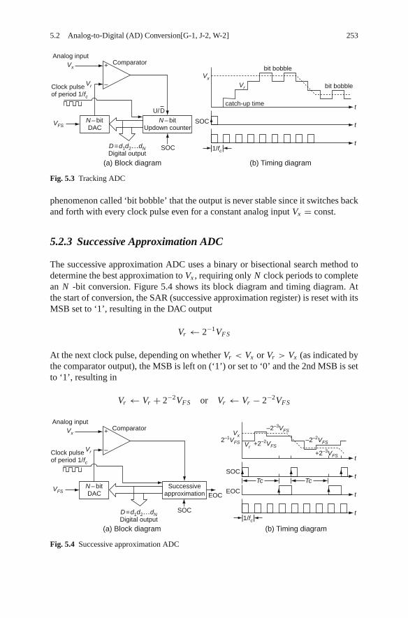
5.2 Analog-to-Digital (AD) Conversion[G-1, J-2, W-2] 253
Analog input
Clock pulseof period 1/fc
|1/fc|
(a) Block diagram (b) Timing diagram
D = d1d2…dNDigital output
Vx
VFSN – bitDAC
N – bitUpdown counter
SOC
SOC
Comparator+
–
catch-up time
bit bobble
bit bobble
U/D
Vr
Vx
Vr
t
t
t
Fig. 5.3 Tracking ADC
phenomenon called ‘bit bobble’ that the output is never stable since it switches backand forth with every clock pulse even for a constant analog input Vx = const.
5.2.3 Successive Approximation ADC
The successive approximation ADC uses a binary or bisectional search method todetermine the best approximation to Vx , requiring only N clock periods to completean N -bit conversion. Figure 5.4 shows its block diagram and timing diagram. Atthe start of conversion, the SAR (successive approximation register) is reset with itsMSB set to ‘1’, resulting in the DAC output
Vr ← 2−1VF S
At the next clock pulse, depending on whether Vr < Vx or Vr > Vx (as indicated bythe comparator output), the MSB is left on (‘1’) or set to ‘0’ and the 2nd MSB is setto ‘1’, resulting in
Vr ← Vr + 2−2VF S or Vr ← Vr − 2−2VF S
Analog input
Clock pulseof period 1/fc
(a) Block diagram
D = d1d2…dNDigital output
Vx
VFSN – bitDAC
Successiveapproximation
SOC
EOCEOC
Tc
Comparator
Vr
|1/fc|(b) Timing diagram
Vx
Vr2–1VFS +2–2VFS
+2–3VFS
–2–3VFS
–2–2VFS
t
t
+
–
SOCt
t
Tc
Fig. 5.4 Successive approximation ADC

254 5 Sampling and Reconstruction
100
010
110
000
001
010
011
100
101
110
111
001
011
101
111
Fig. 5.5 Binary code sequence of a 3-bit successive approximation DAC
Again, depending on Vr < Vx or Vr > Vx , the 2nd MSB is left on(‘1’) or set to ‘0’and the 3rd MSB is set to ‘1’, resulting in
Vr ← Vr + 2−3VF S or Vr ← Vr − 2−3VF S
When the process has been carried out for every bit, the SAR contains the binarynumber representing Vx and EOC line indicates that digital output is available. Inthis way, the 3-bit successive conversion is completed at the end of N clock periodsfor an N -bit ADC so that we have the A/D conversion time
TC = N/ fc(N clock periods) (5.2.3)
Figure 5.5 shows the binary code sequence of a 3-bit successive approximationDAC.
This type of converter is very popular due to its fast conversion rate. A problemwith the SA ADC is that if the input does not remain constant during the full con-version period, the digital output may not be related to the value of the unknowninput voltage Vx . To avoid this problem, sample-and-hold circuits are usually usedahead of the ADC.
5.2.4 Dual-Ramp ADC
Figure 5.6 shows the organization and operation of the dual-ramp ADC. On the SOCpulse, the counter and RC integrator are reset. Then the analog input Vx , connectedto the integrator input through switch S1, is (negatively) integrated during a fixedtime interval of T1 = 2N / fc. At the end of the integration period, the two switchesS1/S2 are turned off/on, respectively so that the reference input −VF S are connectedto the integrator input through S2. Then the integrator output vo increases until itcrosses zero to make the comparator output change. The length of the deintegrationperiod will be measured as T2 = n2/ fc (n2 clock periods).
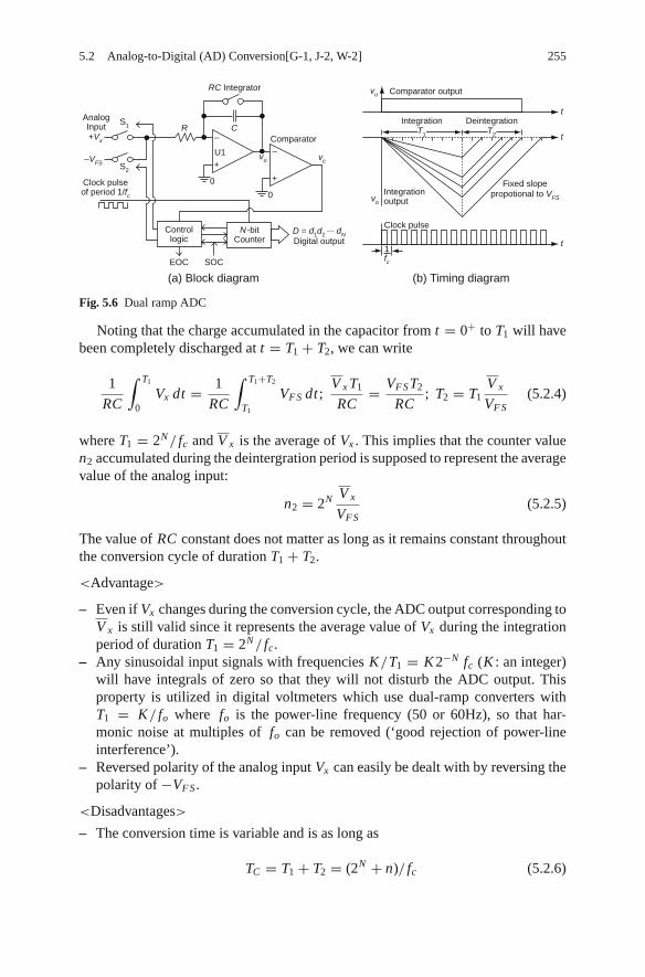
5.2 Analog-to-Digital (AD) Conversion[G-1, J-2, W-2] 255
Comparator outputvo
vo
T1 T2
1fc
t
t
t
Integration
Integrationoutput
Clock pulse
Fixed slopepropotional to VFS
Deintegration
+
–
U1
S1
S2
+
–
RC Integrator
ComparatorC
vo vc
R
D = d1d2 ... dN
Digital output
0
0
+Vx
–VFS
AnalogInput
Clock pulseof period 1/fc
Controllogic
N -bitCounter
SOCEOC
(a) Block diagram (b) Timing diagram
Fig. 5.6 Dual ramp ADC
Noting that the charge accumulated in the capacitor from t = 0+ to T1 will havebeen completely discharged at t = T1 + T2, we can write
1
RC
∫ T1
0Vx dt = 1
RC
∫ T1+T2
T1
VF S dt ;V x T1
RC= VF ST2
RC; T2 = T1
V x
VF S(5.2.4)
where T1 = 2N / fc and V x is the average of Vx . This implies that the counter valuen2 accumulated during the deintergration period is supposed to represent the averagevalue of the analog input:
n2 = 2N V x
VF S(5.2.5)
The value of RC constant does not matter as long as it remains constant throughoutthe conversion cycle of duration T1 + T2.
<Advantage>
– Even if Vx changes during the conversion cycle, the ADC output corresponding toV x is still valid since it represents the average value of Vx during the integrationperiod of duration T1 = 2N / fc.
– Any sinusoidal input signals with frequencies K/T1 = K 2−N fc (K : an integer)will have integrals of zero so that they will not disturb the ADC output. Thisproperty is utilized in digital voltmeters which use dual-ramp converters withT1 = K/ fo where fo is the power-line frequency (50 or 60Hz), so that har-monic noise at multiples of fo can be removed (‘good rejection of power-lineinterference’).
– Reversed polarity of the analog input Vx can easily be dealt with by reversing thepolarity of −VF S .
<Disadvantages>
– The conversion time is variable and is as long as
TC = T1 + T2 = (2N + n)/ fc (5.2.6)
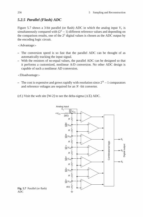
256 5 Sampling and Reconstruction
5.2.5 Parallel (Flash) ADC
Figure 5.7 shows a 3-bit parallel (or flash) ADC in which the analog input Vx issimultaneously compared with (23 − 1) different reference values and depending onthe comparison results, one of the 23 digital values is chosen as the ADC output bythe encoding logic circuit.
<Advantage>
– The conversion speed is so fast that the parallel ADC can be thought of asautomatically tracking the input signal.
– With the resistors of no-equal values, the parallel ADC can be designed so thatit performs a customized, nonlinear A/D conversion. No other ADC design iscapable of such a nonlinear AD conversion.
<Disadvantage>
– The cost is expensive and grows rapidly with resolution since 2N −1 comparatorsand reference voltages are required for an N -bit converter.
(cf.) Visit the web site [W-2] to see the delta-sigma (ΔΣ) ADC.
Fig. 5.7 Parallel (or flash)ADC
+
–
+
–
+
–
+
–
+
–
+
–
+
–
VFS1116
VFS1316
R
VFS916
R
VFS716
R
VFS516
R
VFS316
R
VFS116
R
R/2
3R/2+VFS
d1
d2
d3
Vx
Analog inputC
ombi
nato
rial l
ogic
Dig
ital o
utpu
t

5.3 Sampling 257
5.3 Sampling
5.3.1 Sampling Theorem
In Sect. 3.5.2 we derived the relation between the CTFS Xk of a continuous-timeperiodic signal xP (t) and the N -point DTFS (DFS/DFT) X N (k) of the discrete-timeversion xN [n] = xP (nT ) (obtained by sampling xP (t) every T s), which is periodicwith period N = P/T in n:
X N (k)(3.5.3)= 1
T
∑∞m=−∞ Xk+m N (5.3.1a)
where the frequency components described by the DTFS X N (k) and CTFS Xk arevirtually identical in light of the inter-relationship (1.1.15) between the digital andanalog frequencies:
kΩ0 = k2π
N[rad/sample]
(1.1.15)∼
k2π/N [rad/sample]
T [sec/sample]= k
2π
N T[rad/sec] = k
2π
P= kω0
We also showed that the CTFT Xa(ω) of a continuous-time signal xa(t) is relatedwith the DTFT Xd (Ω) of the discrete-time version xd [n] = xa(nT ) as
Xd (Ω)(3.5.7)= 1
T
∑∞k=−∞ Xa
(ω + k
2π
T
)∣∣∣∣ω=Ω/T
= 1
T
∑∞k=−∞ Xa
(Ω
T+ k
2π
T
)(5.3.1b)
where ω = Ω/T [rad/s] and Ω [rad/sample] are virtually identical in light of theinter-relationship (1.1.15) between the digital and analog frequencies.
Equations (5.3.1a) and (5.3.1b) imply that the DTFS/DTFT of a discrete-timesequence xd [n] = xa(nT ) is qualitatively the periodic extension of the CTFS/CTFTof the continuous-time version xa(t) (with period 2π/T in analog frequency ω or2π in digital frequency Ω), i.e., the sum of infinitely many shifted version of thespectrum of xa(t). This explains how the DTFS/DTFT spectrum of xd [n] = xa(nT )deviates from the CTFS/CTFT spectrum of xa(t) due to frequency-aliasing unlessthe CTFS/CTFT is strictly limited within the low-frequency band of (−π/T, π/T )where T is the sampling interval or period of xd [n] = xa(nT ).
To be more specific, suppose a continuous-time signal xa(t) has a band-limitedCTFT spectrum
Xa(ω) = 0 for |ω| > ωx (5.3.2)
as depicted in Fig. 5.8(a). Then the DTFT spectrum Xd (Ω) of the discrete-time ver-sion xd [n] = xa(nT ), which is the periodic extension of Xa(ω)|ω=Ω/T with period

258 5 Sampling and Reconstruction
Xa(ω)
–ωx ωxω
0
Xd(Ω)
ωx–ωx
0 ππ/T
–π–π/T
2π2π/T
–2π–2π/T
3π3π/T
–3π–3π/T
Ωω=Ω/T
Xd(Ω)
ωx–ωx
0 ππ/T
–π–π/T
–2π–2π/T
Ωω=Ω/T
(c) The spectrum of xd[n]=xa(nT ) with ωs=2π/T < 2ωx
(b) The spectrum of xd[n]=xa(nT ) with ωs=2π/T > 2ωx
(a) The spectrum of xa[t ]
Frequency responseof an ideal LPF
2πωs=2π/T
Fig. 5.8 The spectra of discrete–time signals depending on the sampling frequency – the samplingtheorem
ωs = 2π/T in ω or Ωs = 2π in Ω, is shown in Fig. 5.8(b) and (c) for π/T > ωx
and π/T < ωx , respectively. Notice that Xd (Ω) in the principal frequency range(−π/T, π/T ) is identical to Xa(ω) if
ωs = 2π
T> 2ωx (Nyquist rate) or equivalently,
π
T(folding frequency) > ωx
(5.3.3)where ωx is the highest frequency in xa(t) and ωs = 2π/T and π/T are calledthe sampling frequency and folding or Nyquist frequency, respectively. In this case(Fig. 5.8(b): oversampling), there is no overlap, called aliasing, between adjacentspectral components so that xa(t) or Xa(ω) can be extracted exactly from xd [n] =xa(nT ) or Xd (Ω) by employing an ideal lowpass filter with the magnitude responsedepicted (in a dotted line) in Fig. 5.8(b).
On the other hand, in the case of Fig. 5.8(c) (under-sampling) with π/T < ωx
or equivalently, ωs = 2π/T < 2ωx , the frequency aliasing (or spectral overlap)occurs, producing an irretrievable error in the spectrum. Such an aliasing phe-nomenon makes higher frequencies in Xa(ω) get reflected into lower frequencies,which presents an interpretation of the stroboscopic effect. This effect is occasion-ally observed in films of wagon wheels or aircraft propellers that appear to berotating slower than would be consistent with the forward motion and sometimesin the opposite direction. This story can be summarized as follows:
[Sampling Theorem]In order to retain vital information through sampling with sampling period T ,the sampling frequency ωs = 2π/T must be greater than twice the highest fre-quency ωx contained in the continuous-time signal xa(t) to be sampled, calledthe Nyquist rate 2ωx . Otherwise, i.e., if ωs ≤ 2ωx , the so-called frequencyaliasing effect (spectral overlapping phenomenon) results.

5.3 Sampling 259
When sampling a continuous-time signal xa(t) every T s, we want to ensure thatall the information in the original signal is retained in the samples xd [n] = xa(nT )so that we can exactly recover xa(t) from the discrete-time sequence xd [n]. In thiscontext, the sampling theorem is the most important criterion of the sampling periodselection.
To clarify the concept of aliasing, consider two continuous-time signals x1(t) =sin(2π t) and x2(t) = sin(22π t) shown in Fig. 5.9(a). Each of these signals issampled every T = 0.1 s to give sequences x1[n] = x1(0.1n) = sin(0.2πn)and x2[n] = x2(0.1n) = sin(2.2πn), that are identical. Fig. 5.9(b) also showsthat two continuous-time signals x3(t) = sin(18π t) and x4(t) = − sin(2π t)are sampled every T = 0.1 s to yield x3[n] = x3(0.1n) = sin(1.8πn) andx4[n] = x4(0.1n) = sin(−0.2πn), that are identical. These are examples of fre-quency aliasing that a higher frequency signal, when sampled, appears like a lowerfrequency one.
Figure 5.10 shows the output signals y1(t), y2(t), and y3(t) of an A/D- G[z](digital filter)-D/A structure to the three different input signals where G[z] =(1 − e−1)/(z − e−1). Note that with the sampling period T = 0.1 [s], all theoutputs are of the same digital frequency and that x2(t) = sin(22π t) and x3(t) =sin(18π t) have been aliased/folded with the phase preserved/reversed, respectively.This result can be obtained by running the following program “sig05f10.m” andpredicted from the frequency response of the digital filter G[z], which is shown inFig. 5.11.
0
0.5
–0.5
–1
1
0.2 0.4 0.6 0.8 10 1.2 1.4 1.6 1.8
0
0.5
–0.5
–1
1
0
: x3(0.1n)=sin(1.8πn)x4(t )=–sin(2πt )x3(t )=sin(18πt ) : x4(0.1n)=sin(–0.2πn)
: x1(0.1n)=sin(0.2πn)x2(t )=sin(22πt )x1(t )=sin(2πt ) : x2(0.1n)=sin(2.2πn)
(b) x3[n] and x4[n] obtained by sampling x3(t ) = sin (18πt ) and x4(t ) = sin (–2πt ) with T=0.1
(a) x1[n] and x2[n] obtained by sampling x1(t ) = sin (2πt ) and x2(t ) = sin (22πt ) with T=0.1
t
t0.2 0.4 0.6 0.8 1 1.2 1.4 1.6 1.8
Fig. 5.9 Examples of frequency aliasing/folding or spectral overlap

260 5 Sampling and Reconstruction
t
0
–1
1
0 1t 0
–1
1
0.5 1.50 1 2t
0
–1
1
0.5 1.50 1 2
t0
–1
1
0.5 1.50 1 2
y1(t )
y2(t )
y3(t )
0
–1
1
0.5 1.50 1 2t
0
–1
1
0.5 1.50 1 2t
x1(t )=sin(2πt ) x1(0.1n)=sin(0.2πn)T=0.1
x2(t )=sin(22πt ) x2(0.1n)=sin(2.2πn)T=0.1
T=0.1
x3(t )=sin(18πt ) x3(0.1n)=sin(1.8πn)T=0.1
aliased
folded
A/D G [z] D/A
G [z]=1–e–1
z–e–1
0.5 1.5 2
Fig. 5.10 The effect of frequency aliasing on a system of A/D-G[z]-D/A structure
∠G [z]
–2π –π –0.2π
0.927
–0.92700
(a) The magnitude response of the digital filter G [z]
(b) The phase response of the digital filter G [z]
0 0.2π
10.86 |G [z] |
Ω
Ωπ
π
π 2π–2π –π
–π
1.8π π 2.2π
Fig. 5.11 The frequency response of the digital filter G[z]
%sig05f10.mclear, clfB=[0 1-exp(-1)]; A=[1 -exp(-1)]; % system function of the filterW=[2 22 18]*pi; % the three different frequency of input signalT=0.1; ts=2e-3; % Sampling period, Segment lengthtf=2; t=[0:ts:tf]; n=[0:tf/T]; % Final time, Time rangesx1t= sin(W(1)*t); x1n=x1t([1:T/ts:end]); y1n= filter(B,A,x1n);x2t= sin(W(2)*t); x2n=x2t([1:T/ts:end]); y2n= filter(B,A,x2n);x3t= sin(W(3)*t); x3n=x3t([1:T/ts:end]); y3n= filter(B,A,x3n);subplot(521), plot(t,x1t), hold on, stairs(n*T,x1n,’r’) % Input 1subplot(522), stairs(n*T,y1n) % Output 1

5.3 Sampling 261
subplot(523), plot(t,x2t), hold on, stairs(n*T,x2n,’r’) % Input 2subplot(524), stairs(n*T,y2n) % Output 2subplot(525), plot(t,x3t), hold on, stairs(n*T,x3n,’r’) % Input 3subplot(526), stairs(n*T,y3n) % Output 3% The frequency response of the digital filterW=[-2:0.001:2.3]*pi; GW=freqz(B,A,W);subplot(514), plot(f,abs(GW))subplot(515), plot(f,angle(GW))
Referring to Remark 1.4 (for the physical meaning of the frequency response)and based on the frequency response of the digital filter G[z] depicted in Fig. 5.11,we can write the steady-state response of the digital filter to the digital inputsx1[n] = sin(0.2πn) and x3[n] = sin(1.8πn) as
y1[n] = | G[e jΩ] |∣∣Ω=0.2π
sin(0.2πn + ∠G[e jΩ]∣∣Ω =0.2π
)
= 0.86 sin (0.2πn − 0.927)
y3[n] = | G[e jΩ] |∣∣Ω =1.8π
sin(1.8πn + ∠G[e jΩ]∣∣Ω=1.8π
)
= 0.86 sin (1.8πn + 0.927)
= 0.86 sin (−0.2πn + 0.927) = −0.86 sin (0.2πn − 0.927) = −y1[n]
Here, let us think about how we can interpret the periodicity of the DTFT spectrumof a discrete-time signal and that of the frequency response of a discrete-time sys-tem such as G[z]. The interpretation of the former is an ambiguity that we cannottell which of analog frequency components {(Ω1 ± 2mπ )/T, m: any integer} arecontained in the original continuous-time signal (before sampling with period T ).It should not be interpreted as the existence of infinitely many analog frequencycomponents {(Ω1 ± 2mπ )/T, m: any integer}. On the other hand, the interpre-tation of the latter is an equality that the discrete-time system responds with thesame magnitude and phase of frequency response to the discrete-time version ofcontinuous-time signals of different analog frequencies {(Ω1 ± 2mπ )/T, m: anyinteger}.
There are some rules of thumb for choosing the sampling rate, which are listedin the following remark:
Remark 5.1 Rules of Thumb for Sampling Rate SelectionIn practice, the sampling frequency is chosen to be much higher than the Nyquist
rate. In closed-loop sampled-data systems, low sampling rate has a detrimentaleffect on stability and therefore, the sampling rate selection is made with stabilityconsideration. The rules of thumb are
– to sample 8 ∼ 10 times during a cycle of damped oscillation in the output if thesystem is under-damped or during the rise time of the transient response if thesystem is over-damped, or
– to sample at least 5 times per time constant.

262 5 Sampling and Reconstruction
Remark 5.2 Time Aliasing and Frequency AliasingIn Example 3.15, it can be observed that if the DFT size is not sufficiently
large, in other words, if the sampling rate in the frequency domain [0, 2π ] is notsufficiently high, the aliasing problem may occur in the time domain and such aphenomenon is called the time aliasing. Now in this section, we can observe that alow sampling rate in the time domain may cause the frequency aliasing.
5.3.2 Anti-Aliasing and Anti-Imaging Filters
We know that higher sampling rate satisfies the sampling theorem more easily; inother words, if a continuous-time signal is sampled at a sufficiently high rate, thefrequency-aliasing problem can be alleviated. However, the maximum sampling rateof a S/H (sample/hold device) is upper-bounded by the hardware constraints suchas the delay time of the S/H and the conversion time of A/D (analog-to-digital)converter. If the total conversion time is 1 μs, the maximum sampling rate is 1 MHz.Therefore we may not be able to make the sampling rate as high as we want.Besides, a higher sampling rate increases the number of calculations needed forimplementation.
On the other hand, all physical signals found in the real world are not band-limited and do contain a wide range of frequency components. Besides, an ideallow-pass filter is not realizable. It is therefore impossible to exactly reproduce theoriginal continuous-time signal from its sampled version even though the samplingtheorem is satisfied.
Fortunately, most physical transients tend to be smooth so that their spectra areclose to zero for high frequencies. Still it may be a problem to deal with the signalcorrupted by high-frequency noise. To prevent or reduce aliasing errors caused byundesired high-frequency signals, we must use an analog low-pass filter, called ananti-aliasing prefilter. This filter is applied to the continuous-time signal prior to
(a) The block diagram of a digital signal processing system with anti-aliasing and anti-imaging filters
(b) The frequency responses of an anti-aliasing filter and the overall DSP system
SamplingfrequencyFolding frequency
Guard band0
|Gaa( jω)|
ωc ωs – ωc ωs – 2π /Tω
π /T
G [e jωT ]
Real (analog) world
Anti-aliasingLPF
Gaa(s)
Anti-imaging(Reconstruction)
LPF Gai (s)
Digital FilterG [z]A/D D/Axa(t )
xd [n ] yd [n ]ya(t )
Digital world Real (analog) world
Magnitude response of digital filter G (z )Overall (resulting) magnitude response
Magnitude response of an anti-aliasing filter Gaa(s)
Fig. 5.12 Block diagram and frequency response of a DSP system

5.4 Reconstruction and Interpolation 263
sampling and passes the components with frequencies |ω| ≤ ωc, while attenuat-ing the components with |ω| ≥ ωs − ωc, which would be folded into the range|ω| ≤ ωc. A digital signal processing system using an anti-aliasing LPF and itstypical frequency response are shown in Fig. 5.12. Note that another LPF of similarfrequency characteristic, called an anti-imaging or reconstruction filter, might haveto be installed after D/A conversion to remove unwanted spectral components(above the folding or Nyquist frequency ω f = π/T ) from the DAC output andconstruct a smooth analog output signal.
5.4 Reconstruction and Interpolation
In many practical applications, discrete-time sequences are required to be trans-formed into continuous-time signals. In computer-controlled systems, it is necessaryto convert the control actions calculated by the computer as a sequence of numbersinto a continuous-time signal that can be applied to the plant or process. In digitalaudio compact disk system, the audio signals are stored as digital samples on thedisk and must ultimately be converted into analog signals to drive the speakers. Inthese cases, we are faced with the inverse of the sampling operation, which asks usto think about how to reproduce the analog signal xa(t) from the continuous-timesampled signal x∗(t) = xa(t)δT (t) or discrete-time sequence xd [n] = xa(nT ).
5.4.1 Shannon Reconstruction
We begin by considering the un-aliased spectrum X∗(ω) as shown in Fig. 5.8(b)where X∗(ω) has the same shape with the original spectrum Xa(ω) over the principalfrequency range (−π/T, π/T ) where T is the sampling interval or period. Sup-pose we have an analog lowpass filter (LPF) with the ideal ‘brick wall’ frequencyresponse
G I (ω) ={
T for − π/T ≤ ω ≤ π/T
0 elsewhere(5.4.1)
which passes only frequencies in the range |ω| ≤ π/T and masks out all otherfrequencies. Recall from Eq. (E2.9.2) that
gI (t) = F−1{G I (ω)} (E2.9.2)= TB
πsinc
(Bt
π
)B=π/T= sinc
(t
T
)(5.4.2)
We can apply this filter to X∗(ω) to retrieve the original spectrum Xa(ω) in thefrequency domain as
X (ω) = G I (ω)X∗(ω) (5.4.3)
or in the time domain as

264 5 Sampling and Reconstruction
x(t) = F−1{X (ω)} (2.5.10)= gI (t) ∗ x∗(t)(E2.13.1)= gI (t) ∗ xa(t)δT (t)
(E2.10.1)= gI (t) ∗ xa(t)∑∞
m =−∞ δ(t − mT )
= gI (t) ∗∑∞
m =−∞ xa(t)δ(t − mT ) = gI (t) ∗∑∞
m =−∞ xa(mT )δ(t − mT )
(D.37)=∑∞
m =−∞ xa(mT )gI (t − mT );
x(t)(5.4.2)=
∑∞m =−∞ xa(mT ) sinc
(t − mT
T
)(5.4.4)
The above summation (5.4.4), called Whittaker’s cardinal interpolation formula orWhittaker-Shannon sampling series [S-1, W-1], suggests a reconstruction formula.It can be modified into a more computationally-efficient form
x(t) = sin(π t/T )
π/T
∑∞m =−∞ xa(mT )
(−1)m
t − mT(5.4.5)
where we have used the fact that
sin(π
T(t − mT )
)= sin
(π
Tt)
cos(m π ) − cos(π
Tt)
sin(m π ) = (−1)m sin(π
Tt)
Since the sinc function sinc(t − mT ) has unity value for t = mT and becomes zerofor other Shannon reconstruction sample points, it is obvious that
x(nT ) = xa(nT ) ∀ integer n (5.4.6)
holds for every sample point. The role of gI (t) is to fill in or interpolate the valuesof the continuous-time function between the sample points.
%sig05f13.m
clear, clf
ts=0.001; T=0.1; tt=-0.5:ts:1.4; t0=0; tf=1; % Time range
fs=[0 0.1 0.2 0.3 0.4 0.5]; ws=2*pi*fs/T; % Frequencies contained in x(t)
Aks= [1 1 1 1 1 1]; phiks= [0.5 -0.5 0.5 -0.5 1 -1];
K=6; xt= Aks(1)*sin(ws(1)*tt + phiks(1));
for k=2:K, xt = xt + Aks(k)*sin(ws(k)*tt + phiks(k)); end
nT= tt([1:T/ts:end]); % Sampling point vector
xn= xt([1:T/ts:end]); % Discrete-time sequence sampled with T=0.1
sincmT= inline(’sinc(t/T)’,’t’,’T’);
plot(tt,xt), hold on, stem(nT,xn)
xht= 0;
for n=1:length(xn)
xn sincnT = xn(n)*sincmT(tt-nT(n),T); xht = xht + xn sincnT; %Eq.(5.4.4)
plot(tt,xn sincnT,’:’)
end
plot(tt,xht,’r’), set(gca,’XLim’,[t0 tf],’fontsize’,9)

5.4 Reconstruction and Interpolation 265
3
2
1
0
–1
–2
–3
0 0.5 1t
4
2
3
1
0
–1
–2
–3
0 0.5 1t
: xa(t ): xa(mT )sinc (t–mT ): x (t )^
x (t )^
x (t )^
xa(t )
xa(t )
(b) An example of Whittaker–Shannon reconstruction when the precondition of the sampling theorem is not satisfied
(a) An example of Whittaker–Shannon reconstruction when the precondition of the sampling theorem is satisfied
Fig. 5.13 Examples of Whittaker–Shannon reconstruction
Interested readers are recommended to run the above program “sig05f13.m”twice, once with the number of frequencies K = 5 and once with K = 6, to getFig. 5.13(a) and (b), respectively and then, think about what the difference comesfrom in connection with the precondition of the sampling theorem.
5.4.2 DFS Reconstruction
Recall again the relationship (5.3.1a) between the CTFS Xk of a continuous-timeperiodic signal xP (t) and the N -point DTFS (DFS/DFT) X N (k) of the discrete-timeversion xN [n] = xP (nT ) (obtained by sampling xP (t) every T s), which is periodicwith period N = P/T in n:
X N (k)(3.5.3) or (5.3.1a)= 1
T
∑∞m=−∞ Xk+m N (5.4.7)
This implies that if xP (t) does not contain the frequencies above the foldingfrequency, i.e., half the sampling frequency

266 5 Sampling and Reconstruction
ω f = ωs
2= π
T= N
2
2π
N T
= N
2
2π
P= N
2ω0(corresponding to the frequency index k = N
2)
so that
Xk = 0 ∀ |k| ≥ N
2(5.4.8)
then Eq. (5.4.7) becomes
X N (k)(5.4.7) with (5.4.8)= 1
TXk for |k| <
N
2(5.4.9)
This suggests another reconstruction formula, called the DFS reconstruction, whichis similar to the inverse DFS formula (3.4.8):
x(t) = 1
N
∑| k|<N/2
X N (k)e j2πkt/N T (5.4.10)
%sig05f14.mclear, clfts=0.001; T=0.1; tt=-0.5:ts:1.4; t0=0; tf=1;fs=[0 0.1 0.2 0.3 0.4 0.5]; ws=2*pi*fs/T; % Frequencies contained in x(t)Aks= [1 1 1 1 1 1]; phiks= [0.5 -0.5 0.5 -0.5 1 -1];K=5; xt= Aks(1)*sin(ws(1)*tt + phiks(1));for k=2:K, xt = xt + Aks(k)*sin(ws(k)*tt + phiks(k)); endnT= tt([1:T/ts:end]); xn= xt([1:T/ts:end]);xn causal=[xn(6:end) xn(1:5)]; Xk= fft(xn causal); N=length(Xk);plot(tt,xt), hold on, stem(nT,xn)kk1=[1:N/2].’;xht1 DFS= real(Xk(kk1)*exp(j*2*pi/N/T*(kk1-1)*tt))/N;kk2=[N/2+2:N].’;xht2 DFS= real(Xk(kk2)*exp(j*2*pi/N/T*(kk2-1-N)*tt))/N;xht DFS = xht1 DFS + xht2 DFS;plot(tt,xht DFS,’r’), set(gca,’XLim’,[t0 tf],’fontsize’,9)
Interested readers are recommended to run the above program “sig05f14.m”twice, once with the number of frequencies K = 5 and once with K = 6, to getFig. 5.14(a) and (b), respectively and then, think about what the difference comesfrom in connection with the precondition of the sampling theorem.

5.4 Reconstruction and Interpolation 267
t
(b) An example of Fourier series reconstruction when the precondition of the sampling theorem is not satisfied
(a) An example of Fourier series reconstruction when the precondition of the sampling theorem is satisfied
t
2
1
0
–1
–2
0.5
x (t )^xa(t )
: xa(t )
: x (t )^
Overlapped
2
0
–2
0.5
0
0
x (t )^
xa(t )
Fig. 5.14 Examples of Fourier series reconstruction
5.4.3 Practical Reconstruction
The problem with the ideal (Whittaker-Shannon) interpolation function gI (t) =sinc(t/T ) is that it extends in time from t = −∞ to +∞ and accordingly, it incor-porates the entire sequence of xa(nT ) including all the future samples (for n > 0)as well as all the past samples (for n < 0) to find the estimate of x(t). Besides, incontrol situations we cannot usually wait to observe the entire sequence before aninterpolation is performed. In this section we consider a practical interpolator calledthe zero-order hold (z.o.h.), which is a causal lowpass filter to approximate a signalbetween two consecutive sampling instants nT and (n + 1)T by a constant xa(nT ).This is the beginning of the story about the ideal S/H (sample-and-hold device). Asdepicted in Fig. 5.15(a), the output of a z.o.h. to an input x(t) can be described as
x(t) =∑∞
n=0xa(nT ) (us(t − nT ) − us(t − nT − T )) (5.4.11)
whose Laplace transform is
X (s)(5.4.11)=
B.8(3), B.7(2)
∑∞n=0
xa(nT )
(1
se−nT s − 1
se−nT s−T s
)
=∑∞
n=0xa(nT )e−nT s 1
s(1 − e−T s); (5.4.12)
X (s) = X∗(s) Gh0(s) (5.4.13)

268 5 Sampling and Reconstruction
t
ω
0
0
: Input to S/H: Output from S/H
Gh0( jω)z.o.h. Gh0(s)
S/Hxa(t ) x (t )
xa(t ) x*(t )
X*(s)
x (t )
0
(a) The input and output of a S/H
(b) The magnitude response of a z.o.h.
(c) A S/H and its model
Fig. 5.15 S/H (Sample–and–Hold) modeled by combining an ideal sampler and a z.o.h.
where
X∗(s) = L{x∗(t)} (E2.13.1)= L{
xa(t)∑∞
n=−∞ δ(t − nT )}
B.8(2)=∑∞
n=−∞ xa(nT )e−nT s (4.1.1)= Xd [z]|z=esT (5.4.14)
Gh0(s)(5.4.13)= X (s)
X∗(s)(5.4.12)=(5.4.14)
1
s(1 − e−T s) (5.4.15)
Note that in Eq. (5.4.13) describing the Laplace transform of the z.o.h. output,X∗(s) is the Laplace transform of x∗(t) = xa(t)δT (t) (the output of an ideal samplerto xa(t)), called the starred transform of xa(t). On the other hand, Gh0(s) can beregarded as the system or transfer function of the z.o.h. device since it does notdepend on xa(t). Hence the frequency response of the z.o.h. is
Gh0( jω) = Gh0(s)|s= jω = 1
jω(1 − e− jωT ) = e jωT/2 − e− jωT/2
jωe− jωT/2
= Tsin(ωT/2)
ωT/2e− jωT/2 (5.4.16)
which implies that the z.o.h. is a kind of lowpass filter (see Fig. 5.15(b)). Note thatx∗(t) is not present in physical systems, but it appears in the mathematical modelas a result of factoring and can be considered to be the output of an ideal sampler.Although the ideal sampler and the z.o.h. do not individually model a physical sam-pler and a physical data hold, their combination does accurately model a physicalS/H device (see Fig. 5.15(c)).
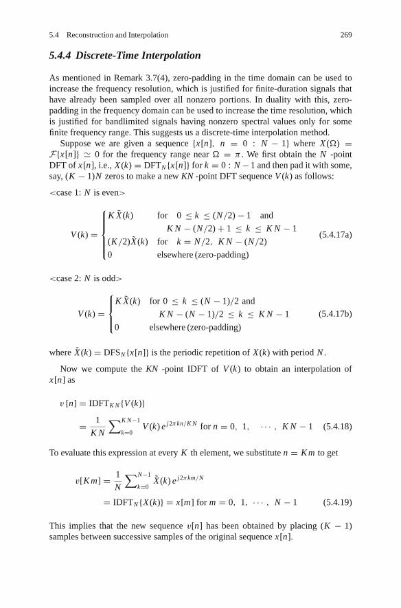
5.4 Reconstruction and Interpolation 269
5.4.4 Discrete-Time Interpolation
As mentioned in Remark 3.7(4), zero-padding in the time domain can be used toincrease the frequency resolution, which is justified for finite-duration signals thathave already been sampled over all nonzero portions. In duality with this, zero-padding in the frequency domain can be used to increase the time resolution, whichis justified for bandlimited signals having nonzero spectral values only for somefinite frequency range. This suggests us a discrete-time interpolation method.
Suppose we are given a sequence {x[n], n = 0 : N − 1} where X (Ω) =F{x[n]} � 0 for the frequency range near Ω = π . We first obtain the N -pointDFT of x[n], i.e., X (k) = DFTN {x[n]} for k = 0 : N −1 and then pad it with some,say, (K − 1)N zeros to make a new KN -point DFT sequence V (k) as follows:
<case 1: N is even>
V (k) =
⎧⎪⎪⎪⎨⎪⎪⎪⎩
K X (k) for 0 ≤ k ≤ (N/2) − 1 and
K N − (N/2) + 1 ≤ k ≤ K N − 1
(K/2)X (k) for k = N/2, K N − (N/2)
0 elsewhere (zero-padding)
(5.4.17a)
<case 2: N is odd>
V (k) =
⎧⎪⎨⎪⎩
K X (k) for 0 ≤ k ≤ (N − 1)/2 and
K N − (N − 1)/2 ≤ k ≤ K N − 1
0 elsewhere (zero-padding)
(5.4.17b)
where X (k) = DFSN {x[n]} is the periodic repetition of X (k) with period N .
Now we compute the KN -point IDFT of V (k) to obtain an interpolation ofx[n] as
v [n] = IDFTK N {V (k)}
= 1
K N
∑K N−1
k=0V (k) e j2πkn/K N for n = 0, 1, · · · , K N − 1 (5.4.18)
To evaluate this expression at every K th element, we substitute n = K m to get
v[K m] = 1
N
∑N−1
k=0X (k) e j2πkm/N
= IDFTN {X (k)} = x[m] for m = 0, 1, · · · , N − 1 (5.4.19)
This implies that the new sequence v[n] has been obtained by placing (K − 1)samples between successive samples of the original sequence x[n].

270 5 Sampling and Reconstruction
(Q) In the case where x[n] is a real-valued sequence, it seems that we need toensure the conjugate symmetry of its K N -point DFT V (k) by modifying a part ofEq. (5.4.17a) as
V (k) ={
(K/2)X (k) for k = N/2
(K/2)X∗(k) for k = K N − (N/2)(5.4.20)
However, we do not have to take the complex conjugate of X (N/2) since it is realfor a real-valued sequence x[n].
Remark 5.3 Discrete-Time Interpolation, Zero Insertion, and Lowpass FilteringThe DFT sequence V (k) is the same as the DFT of the output sequence of an
ideal lowpass filter (with gain K and bandwidth π/K ) to the input signal x(K )[n],which is obtained by inserting (K − 1) zeros between successive sample points ofx[n]. From Eq. (3.2.14), we know that the K N -point DFT of x(K )[n] is
X K N (k) = X N (k) for k = 0, 1, · · · , (K N − 1) :
the periodic repetition of X (k) with period N
Note that Eq. (5.4.17) is equivalent to taking a scaled version of X K (k) within thelow frequency band, which corresponds to a lowpass filtering (see Fig. 5.16(b2)).
Example 5.1 Discrete-Time InterpolationLet us find a discrete-time interpolation for the following sequence (see
Fig. 5.16(a1)):
x [n]n=0
= {2,11,
20,
31} (E5.1.1)
We first compute the N = 4 -point DFT of x[n] as (see Fig. 5.16(b1))
X (k) = DFTN {x[n]} =∑N−1
n=0x[n] e− j2πnk/N =
∑3
n=0x[n] (− j)nk
= x [0] + x [1] (− j)k + x [2] (− j)2k + x [3] (− j)3k
= 2 + (− j)k + (− j)3k ;
X (k) = {4, 2, 0, 2} (E5.1.2)
Then we use Eq. (5.4.17) with K = 2 to get V (k) as (see Fig. 5.16(b3))
V (k)k=0
= {8,14,
20,
30,
40,
50,
60,
74} (E5.1.3)
Now, we compute the K N = 8 -point IDFT of V (k) to obtain the interpolatedsequence v[n] (see Fig. 5.16(a3)):

5.4 Reconstruction and Interpolation 271
n
2
1
00
0 1 2 3
1x [n]
(a1) x [n]
k
4
2
00
0 1 2 3
1X (k )
(b1) X (k )=DFT{x [n]}
n
2
1
00 2
04
03
05
07
01 6
1x (2)[n]
(a2) x (2)[n]: zero–inserted
k
444 4
2
7
2
5
2
3 4
2
10
2
–1
2
–3–4
2
–506
02
0–2
(b2) X~
(k): a periodic repetition of X (k)
n
2
1
00 2
04
0.3
3
0.3
5
1.7
7
1.7
1 6
1v [n]
(a3) v [n]: lowpass–filtered
k
8
00 2
00 0 0 043 5
4
7
4
1 6(b3) V (k): zero–padded
X~
(k)
Zero–insertion
Lowpass–filtering
IDFT
DFT
Ideal LPF frequency response
Zer
o-pa
ddin
g
up-s
ampl
ing
dow
n-sa
mpl
ing
(dec
imat
ion)
Fig. 5.16 Discrete-time interpolation of a discrete-time sequence
v [n] = IDFTK N {V (k)} = 1
8
∑7
k=0V (k) e j2πk n/8
= 1
8(8 + 4e jπkn/4 + 4e− jπkn/4) = 1 + cos
(1
4kπn
);
v [n]n=0
= {2,1
1.707,21,
30.293,
40,
50.293,
61,
71.707}
(E5.1.4)
This result can also be obtained by using the MATLAB routine ‘interpolationdiscrete()’, which implements the procedure described by Eq. (5.4.17)and (5.4.18).
>>x=[2 1 0 1]; K=2;>>v=interpolation discrete(x,K)
2.0000 1.7071 1.0000 0.2929 0 0.2929 1.0000 1.7071
function [xi,Xi]=interpolation discrete(x,K)% To find the KN-point discrete-time interpolation xi of an N-point% discrete-time sequence x[n]N=length(x); KN=K*N; N1=floor((N+1)/2); KNN1=KN-N1+2;X= fft(x);Xi= K*X(1:N1); Xi(KNN1:KN)=K*X(N-N1+2:N); % Eq.(5.4.17)if mod(N,2)==0, Xi([N/2+1 KN-N/2])=K/2*X(N/2+1)*[1 1]; end % Eq.(5.4.17b)xi= ifft(Xi); % Eq. (5.4.18)

272 5 Sampling and Reconstruction
5.5 Sample-and-Hold (S/H) Operation
In a majority of practical digital operations, a S/H function is performed by asingle device consisting of a capacitor, an electronic switch, and operational ampli-fiers, which stores the (sampled) input signal voltage as a charge on the capacitor(Fig. 5.17). OP amps are needed for isolation; capacitor and switch are not con-nected directly to analog circuitry lest the capacitor should affect the input waveformand should be discharged to the output. The mathematical model for a S/H deviceor operation has been developed in Sect. 5.4.3.
Fig. 5.17 Sample-and-Hold(S/H) device
input U1
CTvo
vo
+
–
Vx
U1+
–
The DAC described in Sect. 5.1 may be regarded as a device which consistsof a decoder and an S/H unit (Fig. 5.18(a)). Note that the sampling operationis not necessary, but it is included since the S/H is usually considered as oneunit. The ADC performs the operations of S/H, quantization, and encoding (seeFig. 5.18(b)).
Digital signal
Digital
signal
Analog
signal
Analog signalDAC
Decoder S/H
(b) A model for ADC(a) A model for DAC
Digital signal
Digital
signal
Analog
signal S/H Quantizer Encoder
ADCAnalog signal
Fig. 5.18 Models for DAC and ADC
5.6 Summary
In this chapter we were concerned how continuous-time and discrete-time signalsare and can be related. First, we have included a survey of D/A and A/D conver-sion methods to let the readers know the relationship between analog signals andthe corresponding digital ones and further, to provide them with some practicalinformation that may be useful for the selection of DAC and ADC. Then we dis-cussed the sampling theorem, several reconstruction/interpolation techniques, andthe mathematical model of a practical S/H device.

Problems 273
Problems
5.1 CTFS, DTFS, and Sampling TheoremConsider the following five cosine waves:
x1(t) = cos(2π t) = 1
2(e j2π t + e− j2π t )
x2(t) = cos(8π t) = 1
2(e j8π t + e− j8π t )
x3(t) = cos(10π t) = 1
2(e j10π t + e− j10π t )
x4(t) = cos(18π t) = 1
2(e j18π t + e− j18π t )
x5(t) = cos(22π t) = 1
2(e j22π t + e− j22π t )
(a) Referring to the Fourier representation formula (2.1.5a), verify that theFourier series coefficients of the two-tone signal xa(t) = x1(t) + x2(t)with period Pa = max{2π/2π, 2π/8π} = 1 and fundamental frequencyω0 = 2π are
Xa,k = 1
2,
1
2,
1
2, and
1
2for k = −4,−1 ,+1 , and + 4, respectively.
(P5.1.1)Also for the sequence {xa(nT ), n = 0 : 9} obtained by sampling one periodof the signal with sampling period T = 0.1, find the N = 10 -point DFTX (k) and discuss how it is related with Xa,k based on the relationship (3.5.3)between the CTFS and DTFS. Note that xa(nT ) can be written as
xa[n] = xa(nT ) = 1
2(e j2π n/10 + e− j2πn/10) + 1
2(e j8πn/10 + e− j8πn/10)
(P5.1.2)and it can somehow be matched with the IDFT formula
x [n] = IDFTN {X (k)} (3.4.3)= 1
N
∑N−1
k=0X (k) e j 2πk n/N for n = 0 : N − 1
to yield the DFT coefficients X (k).(b) For xb(t) = x1(t) + x3(t), do the same job as in (a).(c) For xc(t) = x1(t) + x4(t), do the same job as in (a).(d) For xd (t) = x1(t) + x5(t), do the same job as in (a).(e) Complete the following MATLAB program “sig05p 01.m” and run it to
find the N = 10 -point DFTs for {xa(nT ), n = 0 : 9}, {xb(nT ), n = 0 :9}, {xc(nT ), n = 0 : 9}, and {xd (nT ), n = 0 : 9}. Do they agree withthose obtained in (a)–(d)? For each of the four cases (a)–(d), tell whetherthe frequency folding or aliasing occurs or not by the sampling with periodT = 0.1.

274 5 Sampling and Reconstruction
%sig05p 01.mclear, clfws=[2*pi 8*pi 10*pi 18*pi 22*pi];P=1; ts=0.001; tt=[0:ts:P]; T=0.1; N=round(P/T);n=[0:T/ts:length(tt)]; n=n(1:N); nT=n*ts; k=[0:N-1];x1t= cos(ws(1)*tt)+cos(ws(2)*tt); x1n= x1t(n+1); X1= fft(x1n);subplot(521), plot(tt,x1t), hold on, stem(nT,x1n,’.’)subplot(522), stem(k,abs(X1),’.’).. .. .. .. .. ..
(f) Among the sampling rates {15Hz, 20Hz, 25Hz, 40Hz, 50Hz}, choose thelowest one such that the frequency aliasing does not occur for any of (a)–(d).
5.2 ReconstructionConsider the continuous-time waveform x(t) depicted in Fig. P5.2.
–1 0 1t
x (t ) 1
Fig. P5.2
(a) Use Eq. (E2.3.4) to find the CTFT of x(t).(b) Regarding x(t) as a periodic waveform with period P = 2 [s], we can
sample it with sampling period T = 0.5 [s] to get a (non-causal) discrete-time sequence
xNC [n] =n={ −1
0.5,01,
10.5,
20 } (P5.2.1)
and take the part of the periodic repetition of xNC [n] with period N = 4for n = 0 : 3 to have a causal sequence
x [n] =n={ 0
1,1
0.5,20,
30.5} (P5.2.2)
Find the 4-point DFT of this sequence.(c) Find the analytical expression of the DFS reconstruction of x(t) using the
DFT obtained in (b) and plot it on Fig. P5.2.(d) Suppose we can apply an ideal LPF for reconstruction. Can the waveform
depicted in P5.2 be reconstructed perfectly from its sampled version withsome sampling period? Say ‘yes’ or ‘no’ and state the background of youranswer.

Problems 275
5.3 Discrete-Time InterpolationConsider the discrete-time signal x[n] whose DTFT spectrum is depicted inFig. P5.3.
(a) Sketch the spectrum of y[n] = x(2)[n] where
y[n] = x(2)[n] ={
x[n/2] for n = 2m(m : integer)
0 elsewhere(P5.3.1)
(b) Suppose that we wish to form an interpolated version of x[n] by passingy[n] through a lowpass filter. Specify the requirements of the LPF on itsgain and bandwidth.
0–2π
X(Ω)
Ω–π 2ππ
Fig. P5.3
5.4 Discrete-Time InterpolationConsider the discrete-time signal x[n] obtained by sampling the followingcontinuous-time signal x(t) at t = nT (n = 0 : 50, T = 0.0001 sec) withsampling rate Fs = 10kHz.:
x(t) = cos(2π × 1000t) + sin(2π × 3000t) (P5.4.1)
Using the discrete-time interpolation introduced in Sect. 5.4.4, insert 19 pointsbetween successive sample points of x[n] to make a 1020-point interpolationv[n] and plot it (continuously in a solid line) together with x(nT ) (discretelyusing the ‘x’ mark).
5.5 A/D- G[z] (digital filter)-D/A StructureConsider the A/D- G[z] -D/A structure with G[z] = 1 + z−1 where the input isto be sampled with sampling period T = 0.1 [s].
(a) Let the input be given by x1(t) = sin(10π t/3). What is the digital frequencyof x1[n] = x1(nT )?
(b) What is the highest analog frequency such that the input signal will not bealiased?
(c) Find the frequency response and DC gain of the digital filter G[z].(d) Find the steady-state output y1,ss[n] to x1[n] = x1(nT ) = sin(10πT n/3).(e) Find the steady-state output y2,ss[n] to the unit step input x2[n] = us[n].(f) Support your answers to (d) and (e) by the simulations for n = 0 : 50.

Chapter 6Continuous-Time Systems and Discrete-TimeSystems
Contents
6.1 Concept of Discrete-Time Equivalent . . . . . . . . . . . . . . . . . . . . . . . . . . . . . . . . . . . . . . . . . 2776.2 Input-Invariant Transformation . . . . . . . . . . . . . . . . . . . . . . . . . . . . . . . . . . . . . . . . . . . . . . . 280
6.2.1 Impulse-Invariant Transformation . . . . . . . . . . . . . . . . . . . . . . . . . . . . . . . . . . . . . 2816.2.2 Step-Invariant Transformation . . . . . . . . . . . . . . . . . . . . . . . . . . . . . . . . . . . . . . . . 282
6.3 Various Discretization Methods [P-1] . . . . . . . . . . . . . . . . . . . . . . . . . . . . . . . . . . . . . . . . . 2846.3.1 Backward Difference Rule on Numerical Differentiation . . . . . . . . . . . . . . . . . . 2846.3.2 Forward Difference Rule on Numerical Differentiation . . . . . . . . . . . . . . . . . . . . 2866.3.3 Left-Side (Rectangular) Rule on Numerical Integration . . . . . . . . . . . . . . . . . . . 2876.3.4 Right-Side (Rectangular) Rule on Numerical Integration . . . . . . . . . . . . . . . . . . 2886.3.5 Bilinear Transformation (BLT) – Trapezoidal Rule on Numerical Integration . 2886.3.6 Pole-Zero Mapping – Matched z-Transform [F-1] . . . . . . . . . . . . . . . . . . . . . . . . 2926.3.7 Transport Delay – Dead Time . . . . . . . . . . . . . . . . . . . . . . . . . . . . . . . . . . . . . . . . . 293
6.4 Time and Frequency Responses of Discrete-Time Equivalents . . . . . . . . . . . . . . . . . . . . . 2936.5 Relationship Between s-Plane Poles and z-Plane Poles . . . . . . . . . . . . . . . . . . . . . . . . . . . 2956.6 The Starred Transform and Pulse Transfer Function . . . . . . . . . . . . . . . . . . . . . . . . . . . . . 297
6.6.1 The Starred Transform . . . . . . . . . . . . . . . . . . . . . . . . . . . . . . . . . . . . . . . . . . . . . . . 2976.6.2 The Pulse Transfer Function . . . . . . . . . . . . . . . . . . . . . . . . . . . . . . . . . . . . . . . . . . 2986.6.3 Transfer Function of Cascaded Sampled-Data System . . . . . . . . . . . . . . . . . . . . 2996.6.4 Transfer Function of System in A/D-G[z]-D/A Structure . . . . . . . . . . . . . . . . . . 300Problems . . . . . . . . . . . . . . . . . . . . . . . . . . . . . . . . . . . . . . . . . . . . . . . . . . . . . . . . . . . . . . . . . 301
In this chapter we are concerned how continuous-time and discrete-time systemsare or can be related with each other. We will discuss the concept and criterionof discrete-time equivalent (digital simulator) and investigate various discretizationmethods to obtain the discrete-time equivalent for a given analog system, which canbe used for the analysis and design of sampled-data systems.
6.1 Concept of Discrete-Time Equivalent
As the technology of digital processors becomes more advanced, it is often desirableto replace analog systems with digital ones. In some cases, we need to transformthe analog systems into their “equivalent” digital systems in order to simulate theirbehaviors on digital computers. In other cases, rather than designing directly a
W.Y. Yang et al., Signals and Systems with MATLAB R©,DOI 10.1007/978-3-540-92954-3 6, C© Springer-Verlag Berlin Heidelberg 2009
277

278 6 Continuous-Time Systems and Discrete-Time Systems
digital system, we make use of a variety of well-developed analog system designprocedures to get an analog system with satisfactory performance and then convertit into a discrete-time equivalent that mimicks (emulates) the analog system. Ineither case, for a given continuous-time linear time-invariant (LTI) system G A(s)with input x(t) and output yA(t), we wish to find a discrete-time system G D[z] withinput x[n] and output yD[n] such that
x[n] = x(nT ) ⇒ yD[n] = yA(nT ) (6.1.1)
This means that G A(s) and G D[z] yield the equivalent outputs to equivalent inputsin the discrete-time domain. We will call such a system G D[z] the discrete-time(z-domain) equivalent or digital simulator for G A(s) where Eq. (6.1.1) is referredto as the (discrete-time) equivalence criterion. To establish necessary conditions forthe validity of the above criterion, we shall first consider sinusoidal inputs, whichwill lead to the general case, because an arbitrary signal can be expressed as a linearcombination of sine waves (the Fourier series representation). Suppose the inputx[n] of a discrete-time system G D[z] is the discrete-time version of x(t) = e jωt
sampled with period T , i.e., x[n] = x(nT ) = e jnωT where x(t) is the input to thecontinuous-time system G A(s) (see Fig. 6.1):
x(t) = e jωt Sampling with period T−−−−−−−−−−−−−→ x[n] = x(nT ) = e jnωT (6.1.2)
Then we can use the convolutional input-output relationships (1.2.4)/(1.2.9) ofcontinuous-time/discrete-time LTI systems and the definitions of CTFT and DTFTto write the outputs of G A(s) and G D[z] as
yA(t) =∫ ∞
−∞gA(τ )e jω(t−τ )dτ
(2.2.1a)= G A( jω)e jωt
?−−−−−−→Sampling with period T
yD[n] =∑∞
m=−∞ gD[m]e jω(n−m)T
(3.1.1)= G D[e jωT ]e jnωT
(6.1.3)
where
G A( jω)(2.2.1a)=
∫ ∞
−∞gA(τ )e− jωτ dτ
(A.1)=gA(τ )=0 ∀ τ<0
causal system
G A(s)|s= jω (6.1.4a)
G D[e jωT ](3.1.1)=
∑∞m=−∞ gD[m] e− jm ωT (4.1.1b)=
gD[n]=0 ∀ n<0causal system
G D[z]|z=e jωT (6.1.4b)
x (t )=e jωt
?x (nT )=e
jnωT
GA(s)
GD[z ] yD[n ]=GD[e jωT]e
jnωT
yA(t )=GA( jω)e jωT
yA(nT ) = yD[n]
T
Fig. 6.1 The equivalence criterion between a continuous-time system and a discrete-time system

6.1 Concept of Discrete-Time Equivalent 279
The above equivalence criterion (6.1.1) can be stated in terms of the frequencyresponses of the continuous-time and discrete-time systems as
G D[e jωT ] = G A( jω) (6.1.5)
This is referred to as the frequency-domain discrete-time equivalence criterion.However, this equivalence criterion cannot be satisfied perfectly because the
digital frequency response G D[e jωT ] is periodic in ω (Sect. 3.2.1) while the fre-quency response G A( jω) is not. This implies that we cannot find the discrete-timeequivalent of a continuous-time system that would work for all kinds of inputs. Inprinciple, the criterion (6.1.5) can be satisfied only for the principal frequency range(−π/T,+π/T ) if we restrict the class of inputs into band-limited signals that do notcontain frequencies higher than the folding frequency π/T , i.e., half the samplingfrequency ωs = 2π/T . In this sense, the resulting system G D[z] satisfying thecriterion (6.1.5) is a discrete-time equivalent of G A(s), which is valid only for suchband-limited input signals.
Remark 6.1 Equivalence Criterion and Band-Limitedness Condition
(1) The band-limitedness condition is not so restrictive since we can increase π/Tby decreasing the sampling period T . Furthermore, the condition is desirable inorder for the sampled output y(nT ) to represent y(t) faithfully.
(2) As a matter of fact, the equivalence criterion (6.1.5) cannot be met exactlyeven for the principal frequency range since G D[e jωT ] is a rational function ofe jωT , while G A( jω) is a rational function of jω. For engineering applications,however, approximate equality is good enough.
Now we will discuss the time-sampling method, which determines G D[z] so asto satisfy the criterion (6.1.5) with reasonable accuracy for almost every ω in thefrequency band of the input signal. The basic idea is as follows. Suppose that theinput x(t) and the impulse response gA(t) of the analog (or continuous-time) systemG A(s) are sufficiently smooth, i.e., nearly constant in any interval of length T . Then,letting
gD[n] = T gA(nT ) (6.1.6)
satisfies approximately the equivalence criterion (6.1.1), i.e.,
yD[n] ∼= yA(nT ) for x[n] = x(nT )
since we have

280 6 Continuous-Time Systems and Discrete-Time Systems
yA(nT )(1.2.4)=
∫ ∞
−∞gA(τ )x(t − τ )dτ
∣∣∣∣t=nT
∼=∑∞
m=−∞ T gA(nT )x(nT − mT ) (6.1.7a)
yD[n](1.2.9)=
∑∞m=−∞ gD[m]x[n − m] (6.1.7b)
The condition (6.1.6) can be written in terms of the transforms as
G D[z] = TZ{gA(nT )} = TZ{L−1{G A(s)}|t=nT
}(6.1.8)
Remark 6.2 Time-Sampling Method – Impulse-Invariant TransformationNote that sampling the continuous-time unit impulse δ(t) ∼= (1/T )sinc(t/T )
(Eq. (1.1.33a)) at t = nT (i.e., every T s) yields (1/T )sinc(n)(1.1.35)= (1/T )δ[n].
Then, it is very natural that, in order for G A and G D to be similar, their responses toδ(t) and (1/T )δ[n] should be the same, i.e.,
gA(nT ) = G A{δ(t)}|t=nT ≡ G D
{1
Tδ[n]
}= 1
TG D {δ[n]} = 1
TgD[n] (6.1.9)
where G{x(t)} denotes the output of a system G to an input x(t). This is equivalentto the condition (6.1.6) for the impulse-invariant transformation.
Remark 6.3 Frequency Response Aspect of Impulse-Invariant TransformationIf G A( jω) is negligible for |ω| > π/T (in agreement with the smoothness
conditions about gA(t)), then we can take the DTFT of (6.1.6) and use Eq. (3.5.7)or (5.3.1b) to get
G D(Ω) = F{gD[n]}|Ω=ωT ≡ TF(gA(nT )}(5.3.1b)∼= G A(ω) (6.1.10)
6.2 Input-Invariant Transformation
We will consider the input-invariant transformations that are error-free for specificinput signals. For example, the impulse-invariant/step-invariant transformation isaccurate when the input is an impulse or a step function. If they were accurateonly for the specified inputs, they would be of limited practical value. However,by superposition, an input-invariant transformation gives zero error in response toany linear combination of specified input functions.

6.2 Input-Invariant Transformation 281
6.2.1 Impulse-Invariant Transformation
As mentioned in Remark 6.2, this is identical to the time-sampling method discussedin the previous section. Note that Eq. (6.1.8) can be written as
Z−1
{G D[z] · 1
T
}≡ L−1{G A(s) · 1}|t=nT
gD[n] ∗ 1
Tδ[n]
(1.1.28)= 1
TgD[n] ≡ gA(t)|t=nT
(1.1.21)= gA(t) ∗ δ(t)|t=nT (6.2.1)
This implies that the (impulse) response of the continuous-time system G A(s) to theimpulse input δ(t) is equal to the response of the discrete-time system G D[z] to theinput (1/T )δ[n], which is the sampled version of δ(t).
The procedure to derive the impulse-invariant equivalent Gimp[z] for a givenanalog system G A(s) is as follows:
1. Expand G A(s) into the partial fraction form:
G A(s) =∑N
i=1
Ki
s − si(6.2.2)
2. Replace each term 1/(s − si ) by T/(1 − esi T z−1):
Gimp[z] =∑N
i=1
Ki T
1 − esi T z−1(6.2.3)
Remark 6.4 Mapping of Stability Region by Impulse-Invariant TransformationComparing Eq. (6.2.2) with Eq. (6.2.3), we observe that a pole at s = si in
the s-plane is mapped to z = esi T in the z-plane. Consequently, if and only if si
is in the left half plane (LHP), which is the stable region in the s-plane, then thecorresponding pole is inside the unit circle, which is the stable region in the z-plane(see Fig. 6.2). However, the zeros will not in general be mapped in the same way asthe poles are mapped.
10
5
–5
–10
–10 –5 0 5 10
Im{z }
Re{z }
x
x
1
–1x
x
x
0
1
xx
x
x x
jω s–plane
z–planez=esT
σ
Fig. 6.2 Mapping of poles from the s-plane to the z-plane

282 6 Continuous-Time Systems and Discrete-Time Systems
Remark 6.5 Frequency Transformation by Impulse-Invariant TransformationThe relationship between the analog frequency ωA and the corresponding digital
frequency Ω is linear, that is, Ω = ωAT since
e jΩ ≡evaluation along the unit circle
z = esT s= jωA≡evaluation along the jωA−axis
e jωA T (6.2.4)
Consequently, the shape of the frequency response is preserved. The negative aspectof this linear frequency relationship is that short sampling period T does not removethe frequency-aliasing problem caused by the impulse-invariant transformation (seeFig. 6.8).
Example 6.1 Impulse-Invariant Transformation – Time-Sampling MethodFor a continuous-time system with the system function G A(s) and frequency
response G A( jω) as
G A(s) = a
s + a; G A( jω) = a
jω + a(E6.1.1)
the impulse-invariant transformation yields the following discrete system function
Gimp[z](6.2.3)= a T
1 − e−aT z−1; Gimp[e jωT ] = a T
1 − e−aT e− jωT(E6.1.2)
6.2.2 Step-Invariant Transformation
If we let
Gstep[z] = (1 − z−1)Z{L−1
{1
sG A(s)
}∣∣∣∣t=nT
}(6.2.5)
then it will be an exact discrete-time equivalent of G A(s) for any input composed ofstep functions occurring at sample points. Note that Eq. (6.2.5) can be written as
Z−1
{Gstep[z] · 1
1 − z−1
}= L−1
{1
sG A(s)
}∣∣∣∣t=nT
;
gstep[n] ∗ us[n] = gA(t) ∗ us(t)|t=nT (6.2.6)
This implies that the step response of the continuous-time system G A(s) is equal tothe step response of the discrete-time system Gstep[z] on a sample-by-sample basis.That is why Eq. (6.2.5) is called the step-invariant transformation.
Let us consider the discrete-time error model for G A(s) and Gstep[z] in Fig. 6.3,in which the input to G A(s) is x(t), i.e., the zero-order-hold version of x(t). The
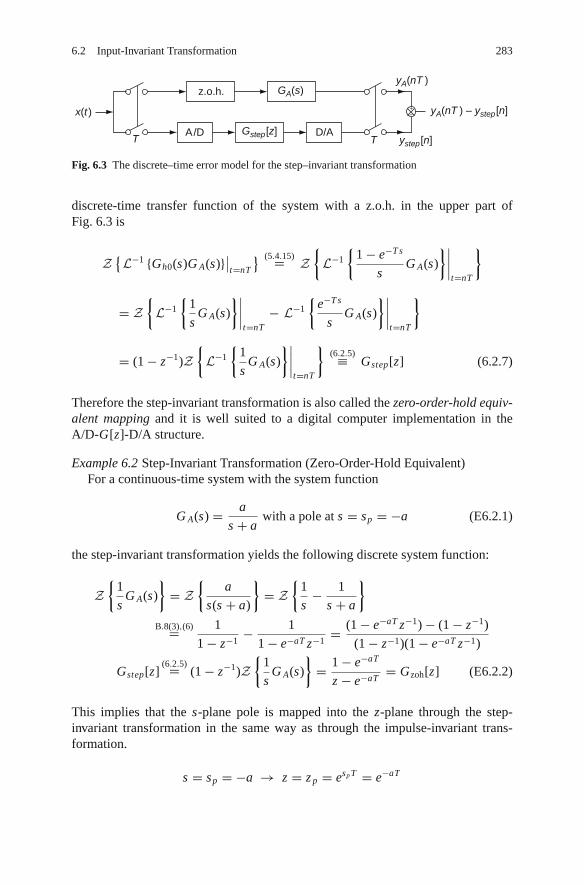
6.2 Input-Invariant Transformation 283
z.o.h.
A/D
x(t )
TGstep[z]
GA(s)yA(nT )
yA(nT ) – ystep[n]
ystep[n]TD/A
+–
Fig. 6.3 The discrete–time error model for the step–invariant transformation
discrete-time transfer function of the system with a z.o.h. in the upper part ofFig. 6.3 is
Z{L−1 {Gh0(s)G A(s)}∣∣t=nT
} (5.4.15)= Z{L−1
{1 − e−T s
sG A(s)
}∣∣∣∣t=nT
}
= Z{L−1
{1
sG A(s)
}∣∣∣∣t=nT
− L−1
{e−T s
sG A(s)
}∣∣∣∣t=nT
}
= (1 − z−1)Z{L−1
{1
sG A(s)
}∣∣∣∣t=nT
}(6.2.5)≡ Gstep[z] (6.2.7)
Therefore the step-invariant transformation is also called the zero-order-hold equiv-alent mapping and it is well suited to a digital computer implementation in theA/D-G[z]-D/A structure.
Example 6.2 Step-Invariant Transformation (Zero-Order-Hold Equivalent)For a continuous-time system with the system function
G A(s) = a
s + awith a pole at s = sp = −a (E6.2.1)
the step-invariant transformation yields the following discrete system function:
Z{
1
sG A(s)
}= Z
{a
s(s + a)
}= Z
{1
s− 1
s + a
}B.8(3),(6)= 1
1 − z−1− 1
1 − e−aT z−1= (1 − e−aT z−1) − (1 − z−1)
(1 − z−1)(1 − e−aT z−1)
Gstep[z](6.2.5)= (1 − z−1)Z
{1
sG A(s)
}= 1 − e−aT
z − e−aT= Gzoh[z] (E6.2.2)
This implies that the s-plane pole is mapped into the z-plane through the step-invariant transformation in the same way as through the impulse-invariant trans-formation.
s = sp = −a → z = z p = esp T = e−aT

284 6 Continuous-Time Systems and Discrete-Time Systems
6.3 Various Discretization Methods [P-1]
A continuous-time LTI system can be described by the system or transfer function as
G A(s) = Y (s)
X (s)
where X (s) and Y (s) are the Laplace transforms of the input and output. Its input-output relationship can be written as an integro-differential equation. We often usethe numerical methods to convert the integro-differential equation into the corre-sponding difference equation, which can easily be solved on a digital computer.The difference equation may be represented by a discrete system function G D[z](Sect. 4.4), which can be thought of representing a discrete-time equivalent to G A(s)(see Fig. 6.4).
Continuous–time system
L
Discrete–time system
Integro–differential equationNumerical
approximation
Discretizations= f (z )
(Laplace transform)
Transfer function
Difference equation
(z–transform) Z
Transfer function
GD[z ] = Y [z ]
X [z ]=
⇔ ⇔
ΣMj = 0
bj z – j
=y [n–i ] x [n–j ]ΣNi = 0
ai ΣMj = 0
bj
ΣNi = 0
ai z – j
i = 0
GA(s) = Y (s)
X (s)=
ΣMj = 0
bj s j
ΣN ai s i
=d i y (t )
dt i
d jx (t )
dt j
ΣNi = 0 ΣM
j = 0ai bj
Fig. 6.4 Discretization and numerical approximation
Some numerical approximation techniques on differentiation/integration willnow be presented with the corresponding discretization methods.
6.3.1 Backward Difference Rule on Numerical Differentiation
We could replace the derivative of a function x(t)
y(t) = d
dtx(t) : Y (s) = s X (s)
by
y(nT ) = x(nT ) − x(nT − T )
T: Y [z] = 1 − z−1
TX [z]
where the initial values have been neglected since we are focusing on describingthe input-output relationship. This numerical differentiation method suggests thebackward difference mapping rule (Fig. 6.5(a)):
s → 1 − z−1
Tor equivalently,
1
1 − s T→ z (6.3.1)

6.3 Various Discretization Methods [P-1] 285
(a) Backward difference rule
0 (n – 1)T
→ y (nT )=
y(t )= x (t )
x (nT ) – x (nT–T )T
ddt
nTt
(c) Mapping of stable region(b) Right–side integration rule
0
→ y (nT )=y (nT–T )+Tx (nT )
(n –1)T nTt
y (t ) = ∫ x (τ)dτt
01
–1
Im{z }
Re{z}
z–plane
0 1/2
–1
1
Fig. 6.5 Backward difference or right–side integration rule
Example 6.3 Backward Difference RuleFor a continuous-time system with the system function G A(s) = a/(s + a), the
backward difference rule yields the following discrete system function:
Gb[z](6.3.1)= a
s + a
∣∣∣∣s=(1−z−1)/T
= a
(1 − z−1)/T + a
= aT
1 + aT − z−1= aT z/(1 + aT )
z − 1/(1 + aT )(E6.3.1)
This implies that the s-plane pole is mapped into the z-plane through the backwarddifference or right-side integration rule as
s = sp = −a → z = z p(6.3.1)= 1
1 − spT
for |sp T |<<1∼=(D.25)
1
e−sp T= esp T (E6.3.2)
This implies that if the s-plane pole sp is so close to the origin and/or the samplingperiod is so short that |spT | << 1, then the location of the pole mapped to thez-plane from the s-plane is
z p∼= esp T
This relationship between the s-plane poles and the corresponding z-plane poles isalmost the same as those for other discretization methods.
Remark 6.6 Mapping of Stability Region and Frequency TransformationFrom Eq. (6.3.1), it can be seen that the jω-axis (the stability boundary) in the
s-plane is mapped to
z = 1
1 − jωT= 1 − jωT + 1 + jωT
2(1 − jωT )= 1
2(1 + e jθ ) with θ = 2 tan−1(ωT )
(6.3.2)
This describes the circle of radius 1/2 and with the center at z = 1/2, which isinside the unit circle in the z-plane (see Fig. 6.5(c)). It is implied that the backward

286 6 Continuous-Time Systems and Discrete-Time Systems
difference rule always maps stable analog systems into stable discrete equivalents,but some unstable analog systems also yield stable discrete ones. Besides, since thejω-axis in the s-plane does not map to the unit circle in the z-plane, the digitalfrequency response will deviate from the analog frequency response as ω → ±∞or Ω → ±π (farther from s = 0 or z = 1). Thus, in order to make the frequencyresponse of the discrete-time equivalent close to that of the original analog system(for the principal frequency range), we must decrease the sampling T or equiva-lently, increase the sampling frequency ωs so that significant pole/zeros are mappedto the neighborhood of z = 1.
6.3.2 Forward Difference Rule on Numerical Differentiation
We could replace the derivative of a function x(t)
y(t) = d
dtx(t) : Y (s) = s X (s)
byy(nT ) = x(nT + T ) − x(nT )
T: Y [z] = z − 1
TX [z]
This numerical differentiation method suggests the forward difference mapping rule(Fig. 6.6(a)):
s → z − 1
Tor equivalently, 1 + s T → z (6.3.3)
Example 6.4 Forward Difference RuleFor a continuous-time system with the system function G A(s) = a/(s + a), the
forward difference rule yields the following discrete system function:
G f [z] = a
s + a
∣∣∣∣s=(z−1)/T
= a
(z − 1)/T + a= aT
z − (1 − aT )(E6.4.1)
→ y (nT )=
0
(a) Forward difference rule (b) Left–side integration rule (c) Mapping of stable region
0
(n+1)T (n – 1)T (n + 1)T
x (nT+T )–x (nT )T
→ y (nT )=y (nT–T )+Tx (nT–T )
nT nTt
Im{z }
Re{z }
z–plane
z=1
t
y (t ) = ∫ x (τ)dτt
0y (t )= x (t )ddt
Fig. 6.6 Forward difference or left–side integration rule

6.3 Various Discretization Methods [P-1] 287
This implies that the s-plane pole is mapped into the z-plane through the forwarddifference or left-side integration rule as
s = sp = −a → z = z p(6.3.3)= 1 + spT
(D.25)∼=for |sp T |<<1
esp T (E6.4.2)
This implies that if the s-plane pole sp is so close to the origin and/or the samplingperiod is so short that |spT | << 1, then the location of the poles mapped to thez-plane from the s-plane is
z p∼= esp T
Remark 6.7 Mapping of Stability Region By Forward Difference RuleFrom Eq. (6.3.3), it can be seen that the jω-axis (the stability boundary) in the
s-plane is mapped to
z = 1 + jωT (6.3.4)
This describes the straight line parallel to the imaginary axis and crossing the realaxis at z = 1. It is implied that the forward difference rule maps the left halfplane (LHP) in the s-plane to the left of z = 1 in the z-plane with some por-tion outside the unit circle. Consequently, some stable analog systems may yieldunstable discrete equivalents, while unstable analog systems always make unsta-ble discrete ones. Hence, this is an undesirable mapping that cannot be used inpractice.
6.3.3 Left-Side (Rectangular) Rule on Numerical Integration
We could replace the integral of a function x(t)
y(t) =∫ t
0x(τ )dτ : Y (s) = 1
sX (s)
byy(nT ) = y(nT − T ) + T x(nT − T ) : Y [z] = T z−1
1 − z−1X [z]
This numerical integration method suggests the left-side integration rule(Fig. 6.6(b)):
s → z − 1
Tor equivalently, 1 + s T → z (6.3.5)
This is identical to the forward difference rule (6.3.3).
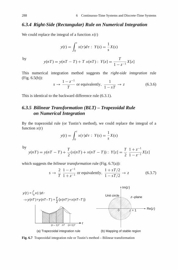
288 6 Continuous-Time Systems and Discrete-Time Systems
6.3.4 Right-Side (Rectangular) Rule on Numerical Integration
We could replace the integral of a function x(t)
y(t) =∫ t
0x(τ )dτ : Y (s) = 1
sX (s)
byy(nT ) = y(nT − T ) + T x(nT ) : Y [z] = T
1 − z−1X [z]
This numerical integration method suggests the right-side integration rule(Fig. 6.5(b)):
s → 1 − z−1
Tor equivalently,
1
1 − sT→ z (6.3.6)
This is identical to the backward difference rule (6.3.1).
6.3.5 Bilinear Transformation (BLT) – Trapezoidal Ruleon Numerical Integration
By the trapezoidal rule (or Tustin’s method), we could replace the integral of afunction x(t)
y(t) =∫ t
0x(τ )dτ : Y (s) = 1
sX (s)
byy(nT ) = y(nT − T ) + T
2(x(nT ) + x(nT − T )) : Y [z] = T
2
1 + z−1
1 − z−1X [z]
which suggests the bilinear transformation rule (Fig. 6.7(a)):
s → 2
T
1 − z−1
1 + z−1or equivalently,
1 + sT/2
1 − sT/2→ z (6.3.7)
→ y (nT )=y (nT–T ) + (x (nT )+x (nT–T ))
y (t ) = ∫ x (τ)dτt
0
(n – 1)T
(a) Trapezoidal integration rule (b) Mapping of stable region
(n+1)T
Im{z }
Re{z }
z–planeUnit circle
t nT
2T
0 z = 1
Fig. 6.7 Trapezoidal integration rule or Tustin’s method – Bilinear transformation

6.3 Various Discretization Methods [P-1] 289
Example 6.5 Bilinear Transformation (BLT)For a continuous-time system with the system function G A(s) = a/(s+a) having
a pole at s = −a and cutoff frequency ωA,c = a, the bilinear transformation (BLT)yields the following discrete system function:
Gbl[z] = a
s + a
∣∣∣∣s= 2(1−z−1)
T (1+z−1)
= a2(1−z−1)T (1+z−1) + a
= aT (z + 1)/(2 + aT )
z − 1−aT/21+aT/2
(E6.5.1)
This implies that the s-plane pole is mapped into the z-plane through the BLT as
s = sp = −a → z = z p(6.3.7)= 1 + spT/2
1 − spT/2= 1 − aT/2
1 + aT/2(E6.5.2)
(= esp T/2
e−sp T/2∼= esp T for |spT | << 1
)
The cutoff frequency of this discrete-time equivalent can be found as
|Gbl [z]||z=e jωT =∣∣∣∣∣ a
2(e jωT/2−e− jωT/2)T (e jωT/2+e− jωT/2) + a
∣∣∣∣∣ =∣∣∣∣∣ a
j 2T tan
(ωT2
) + a
∣∣∣∣∣≡ 1√
2; ωD,c = 2
Ttan−1
(ωA,cT
2
)(E6.5.3)
Remark 6.8 Mapping of Stability Region and Frequency Transformation by BLTFrom Eq. (6.3.7), it can be seen that the jω-axis (the stability boundary) in the
s-plane is mapped to
z(6.3.7)=s= jω
1 + jωT/2
1 − jωT/2=
√12 + (ωT/2)2√12 + (ωT/2)2
<
(tan−1
(ωT
2
)− tan−1
(−ωT
2
))
= e j2 tan(ωT/2) = e jΩ (6.3.8)
which describes the unit circle itself (see Fig. 6.7(b)). It is implied that the BLTalways maps stable/unstable analog systems into stable/unstable discrete-time equiv-alents. However, since the entire jω-axis in the s-plane maps exactly once onto theunit circle in the z-plane, the digital frequency response will be distorted (warped)from the analog frequency response while no frequency aliasing occurs in the fre-quency response, i.e., the analog frequency response in the high frequency rangeis not wrapped up into the digital frequency response in the low frequency (seeFig. 6.8). We set z = e jΩ = e jωD T with Ω = ωDT in Eq. (6.3.8) to get the
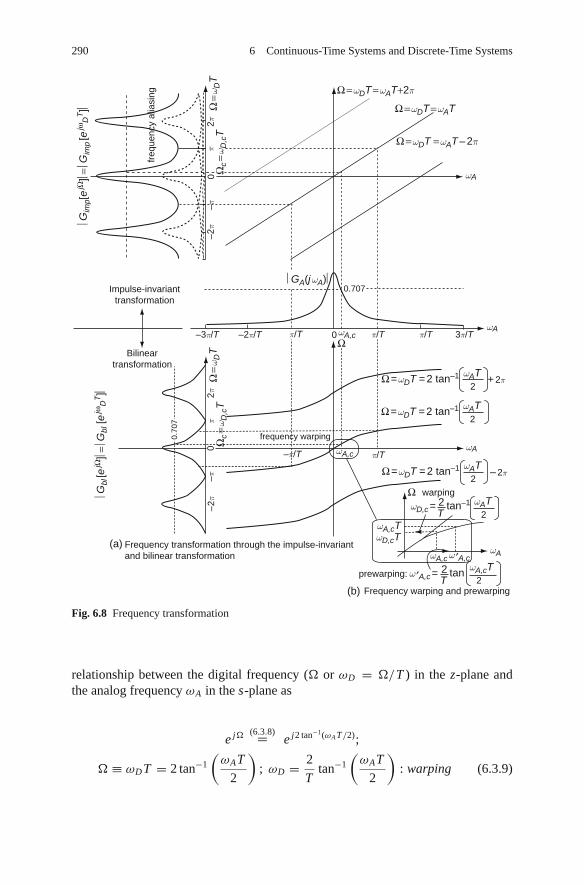
290 6 Continuous-Time Systems and Discrete-Time Systems
⎜Gim
p[e
jΩ]⎜
= ⎜G
imp [e
jωD
T]⎜
ωA,cωA
ωA
ωA
⎜GA(j ωA)⎜
⎜Gbl
[e jΩ
]⎜=
⎜Gbl
[e jω
DT]⎜
–2π
2π0
–ππ
Ω =
ω DT
Ωc =
ω D,c
T–2
π
–3π/T –2π/T
–π/T
0
0.707
π/T
ωA,cTωD,cT
ωA,c ω′A,cωA
π/T
π/T π/T 3π/T
2π0
freq
uenc
y al
iasi
ng
Frequency warping and prewarping
prewarping:
frequency warping
warping
Frequency transformation through the impulse-invariantand bilinear transformation
Impulse-invarianttransformation
Bilineartransformation
–ππ
Ω =
ω DT
Ωc =
ω D,c
T
Ω = ωDT = ωAT+2π
Ω = ωDT = ωAT
ωAT
Ω = ωDT = ωAT – 2π
Ω = ωDT = 2 tan–1
(b)
(a)
Ω
+ 2π2
ωATΩ = ωDT = 2 tan–12
ωAT2
ωATΩ = ωDT = 2 tan–1
ωD,c =
– 2π2
Ω2 tan–1T
ωA,cT2
ω′A,c = 2 tanT
0.70
7
ωA,c
Fig. 6.8 Frequency transformation
relationship between the digital frequency (Ω or ωD = Ω/T ) in the z-plane andthe analog frequency ωA in the s-plane as
e jΩ (6.3.8)= e j2 tan−1(ωA T/2);
Ω ≡ ωDT = 2 tan−1
(ωAT
2
); ωD = 2
Ttan−1
(ωAT
2
): warping (6.3.9)

6.3 Various Discretization Methods [P-1] 291
For low frequencies such that |ωA| << 1 → tan−1(ωAT/2) ∼= ωAT/2, thisrelationship collapses down to
ωD∼= ωA (6.3.10)
On the other hand, the nonlinear compression for high frequencies is more apparent,causing the frequency response at high frequencies to be highly distorted throughthe bilinear transformation.
Remark 6.9 Prewarping
(1) To compensate for the frequency warping so that frequency characteristics ofthe discrete-time equivalent in the frequency range of interest is reasonablysimilar to those of the continuous-time system, we should prewarp the criticalfrequencies before applying the BLT, by
ω′A ← 2
Ttan
(ωAT
2
): prewarping (6.3.11)
so that frequency transformation (6.3.9) with prewarping becomes
ω′D
(6.3.9)= 2
Ttan−1
(ω′
AT
2
)≡ ωA (6.3.12)
(2) The BLT with prewarping at an analog frequency ωc can be performed bysubstituting
s → 2
T
1 − z−1
1 + z−1× ωc
(2/T ) tan(ωcT/2)= ωc
tan(ωcT/2)
1 − z−1
1 + z−1
instead of s → 2
T
1 − z−1
1 + z−1(6.3.13)
for s in G A(s) where ωc(< π/T ) is a critical (prewarp) frequency.(3) The warping and prewarping (against warping) by the frequency scale conver-
sion is depicted in Fig. 6.8. It is implied that, if we design an analog filter,i.e., determine G A( jω′
A) to satisfy the specifications on frequency ω′A, the orig-
inal frequency response specifications on ωA will be satisfied by the digital filterGbl [z] that is to be obtained by applying the BLT to G A(s ′).
Figure 6.8 show the frequency transformation through BLT (accompanied withfrequency warping, but no frequency aliasing) and that through impulse-invarianttransformation (accompanied with frequency aliasing, but no frequency warping).
Example 6.6 Bilinear Transformation with PrewarpingFor a continuous-time system with the system function G A(s) = a/(s+a) having
a pole at s = −a and cutoff frequency ωA,c = a, the bilinear transformation (BLT)with prewarping yields the following discrete system function:

292 6 Continuous-Time Systems and Discrete-Time Systems
Gbl,pre[z](6.3.13)= a
s + a
∣∣∣∣s= a(1−z−1)
tan(aT/2)(1+z−1)
= (2/T ) tan(aT/2)2(1−z−1)T (1+z−1) + 2
T tan(aT/2)(E6.6.1)
This implies that the s-plane pole is mapped into the z-plane through the BLT as
s = sp = −a → z = z p(6.3.13)= 1 + sp tan(aT/2)/a
1 − sp tan(aT/2)/a(∼= 1 − aT/2
1 + aT/2∼= esp T/2
e−sp T/2∼= esp T for |spT | << 1
)(E6.6.2)
Note that G A(s) and its discrete-time equivalent obtained by the BLT with prewarp-ing have the same cutoff frequency (half-power point) ωD = a at which
|G A( jωA)| |ωA=a = ∣∣Gbl,pre[e jωD T ]∣∣∣∣
ωD=a = 1√2
= −3 [dB] (E6.6.3)
6.3.6 Pole-Zero Mapping – Matched z-Transform [F-1]
This technique consists of a set of heuristic rules given below.
(1) All poles and all finite zeros of G A(s) are mapped according to z = esT .(2) All zeros of G A(s) at s = ∞ are mapped to the point z = −1 in G[z]. (Note
that s = j∞ and z = −1 = e jπ represent the highest frequency in the s-planeand in the z-plane, respectively.)
(3) If a unit delay in the digital system is desired for any reason (e.g., because ofcomputation time needed to process each sample), one zero of G A(s) at s = ∞is mapped into z = ∞ so that G[z] is proper, that is, the order of the numeratoris less than that of the denominator.
(4) The DC gain of G pz[z] at z = 1 is chosen to match the DC gain of G A(s) ats = 0 so that
G D[z]|z=e jωp T =1 ≡ G A(s)|s= jωA=0 ; G pz[1] ≡ G A(0)
Example 6.7 Pole-Zero MappingFor a continuous-time system with the system function G A(s) = a/(s + a), we
can apply the pole-zero mapping procedure as
a
s + azero at s = ∞pole at s = −a
Rule 1, 2→ zero at z = −1pole at z = e−aT
z + 1
z − e−aT
Rule 3→ zero at z = ∞,
pole at z = e−aT1
z − e−aT
Rule 4→ G pz[z] = 1 − e−aT
z − e−aT(E6.7.1)

6.4 Time and Frequency Responses of Discrete-Time Equivalents 293
At the last stage, (1−e−aT ) is multiplied so that the DC gain is the same as that of theanalog system: G pz[1] ≡ G A(0) = 1. This happens to be identical with Eq. (E6.2.2),which is obtained through the step-invariant (or z.o.h. equivalent) transformation.
Remark 6.10 DC Gain AdjustmentIrrespective of which transformation method is used, we often adjust the DC gain
of G[z] by multiplying a scaling factor to match the DC steady-stateresponse:
G D[z]|z=e jωp T =1 ≡ G A(s)|s= jωA=0 ; G pz[1] ≡ G A(0) (6.3.14)
6.3.7 Transport Delay – Dead Time
If an analog system contains a pure delay of d s in time, it can be represented by acontinuous-time model of the form
G(s) = H (s)e−sd (6.3.15)
If the time delay is an integer multiple of the sampling period T , say, d = MT ,then the delay factor e−sd = e−sMT can be mapped to z−M (with M poles at z =0). More generally, if we have d = MT + d1 with 0 ≤ d1 < T , then we canwrite
e−sd = e−sMT e−sd1 (6.3.16)
With sufficiently high sampling rate such that d1 < T << 1, we can make a rationalapproximation of
e−d1s ∼= 1 − d1s/2
1 + d1s/2(6.3.17)
Now we can substitute Eq. (6.3.16) with Eq. (6.3.17) into Eq. (6.3.15) and apply adiscretization method to obtain the discrete-time equivalent.
6.4 Time and Frequency Responsesof Discrete-Time Equivalents
In the previous section we have obtained several discrete-time equivalents for thecontinuous-time system G A(s) = a/(s +a). Figure 6.9(a1, a2, b1, and b2) show thetime and frequency responses of the two discrete-time equivalents obtained by thez.o.h. mapping and BLT for the sampling period of T = 0.5 and T = 0.1 [s] wherea = 1. The following program “sig06f09.m” can be used to get Figs. 6.9(a1) and(b1).
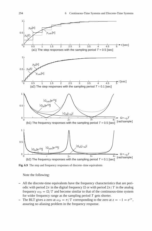
294 6 Continuous-Time Systems and Discrete-Time Systems
Ω = ωDT
Ω = ωDT2π
2π
1
0.5
00
1
0.5
00 0.5 1.51 2 3 4 54.52.5 3.5
1
0.5
00 0.5 1.51 2 3 4 54.52.5 3.5
1
0.5
00 [rad/sample]
[rad/sample]
t [sec]
t [sec]
(b1) The frequency responses with the sampling period T = 0.5 [sec]
(b2) The frequency responses with the sampling period T = 0.1 [sec]
(a2) The step responses with the sampling period T = 0.1 [sec]
(a1) The step responses with the sampling period T = 0.5 [sec]
3π
3π
4π
4π
π
π
⎜GA(j ωA)⎜
⎜GA( j ωA)⎜
⎜Gbl [e jΩ]⎜
ybl[n]
yb l[n]
yzoh[n]
yzoh [n]
yA(t)
yA(t )
⎜Gbl [e jΩ]⎜
⎜Gzoh [e jΩ]⎜
⎜Gzoh [e jΩ]⎜
Fig. 6.9 The step and frequency responses of discrete–time equivalents
Note the following:
– All the discrete-time equivalents have the frequency characteristics that are peri-odic with period 2π in the digital frequency Ω or with period 2π/T in the analogfrequency ωD = Ω/T and become similar to that of the continuous-time systemfor wider frequency range as the sampling period T gets shorter.
– The BLT gives a zero at ωD = π/T corresponding to the zero at z = −1 = e jπ ,assuring no aliasing problem in the frequency response.

6.5 Relationship Between s-Plane Poles and z-Plane Poles 295
– The BLT with prewarping gives the half-power (3dB) frequency at ωD = a justlike the continuous-time system.
%sig06f09.m% Continuous-to-Discrete-time conversion of GA(s)=a/(s+a) with a=1clear, clfa=1; B=1; A=[1 a]; GAs=tf(B,A); % Analog transfer functiont f=5; tt=[0:0.01:t f]; % Time vectorfD=[0:0.001:2]; wD=2*pi*fD; % Digital/Analog frequency vector in HzT=0.5; % Sampling periodfA=fD/T; wA=wD/T; % Digital/Analog frequency vector in rad/sGAw mag= abs(freqs(B,A,wA)); % Analog frequency reponse |GA(jw)|GD zoh=c2d(GAs,T,’zoh’); [Bd zoh,Ad zoh]=tfdata(GD zoh,’v’)GD BLTp=c2d(GAs,T,’prewarp’,a); [Bd BLTp,Ad BLTp]= tfdata(GD BLTp,’v’)[yt,t]=step(GAs,t f); % Step responseN=t f/T; nT=[0:N-1]*T; yn zoh=dstep(Bd zoh,Ad zoh,N);subplot(411), plot(t,yt), hold on, stairs(nT,yn zoh,’:’)GDw zoh mag=abs(freqz(Bd zoh,Ad zoh,wD)); % Digital frequency responsesubplot(413), plot(fD,GAw mag, fD,GDw zoh mag,’:’)
6.5 Relationship Between s-Plane Polesand z-Plane Poles
In this section, we will derive the mathematical relationship between the s-plane andz-plane pole locations. We write the system function of a continuous-time second-order system in standard form as
G(s) = ω2n
s2 + 2ζωns + ω2n
= ω2n
(s + σ )2 + ω2d
, 0 ≤ |ζ | ≤ 1 (6.5.1)
which has the poles at
s1,2 = −ζωn ± j ωn
√1 − ζ 2 = −σ ± j ωd (Fig. 6.10(a))
–ζωn
ωn
θ5 1000
5
10
0 t
fasterdecreasing
high
erfr
eque
ncy
The pole locations of an analog system(a) The impulse response corresponding to the pole locations
(b)
–5
–10
jωd = jωn 1– ζ 2√
Fig. 6.10 Pole locations and the corresponding impulse responses

296 6 Continuous-Time Systems and Discrete-Time Systems
where ζ, σ, ωn , and ωd are the damping ratio, damping constant, natural frequency,and damped frequency. Note that the impulse response of the system is
g(t) = L−1{G(s)} = ωn√1 − ζ 2
e−σ t sin(ωd t) (Fig. 6.10(b)) (6.5.2)
The z-plane poles corresponding to the s-plane poles s1,2 are located at
z1,2 = esT∣∣s1,2
= e−σ T ∠ ± ωd T = r∠ ± Ω (6.5.3)
where
e−ζωn T = e−σ T = r or ζωnT = σ T = − ln r (6.5.4a)
and ωnT√
1 − ζ 2 = ωd T = Ω : digital frequency (6.5.4b)
The discrete-time version of the impulse response can be written as
g[n] = g(nT )(6.5.2)= ωn√
1 − ζ 2e−σ T n sin (ωd T n)
(6.5.4a,b)= ωn√1 − ζ 2
rn sin (Ωn) (6.5.5)
Note that the larger the distance r of a pole from the origin is, the slower the outputstemming from the pole converges; on the other hand, the larger the phase Ω (digitalfrequency) of a pole is, the shorter the discrete-time oscillation period of the outputstemming from the pole Ω is.
Based on Eqs. (6.5.4a) and (6.5.4b), we can express the dampling ratio ζ andnatural frequency ωn in terms of the parameters of the pole location, i.e., the absolutevalue r and phase Ω of the pole(s) as
ζ√1 − ζ 2
= − ln r
Ω; ζ = − ln r√
ln2 r + Ω2(6.5.6)
ωn = 1
T
√ln2 r + Ω2 (6.5.7)
The time constant of the pole(s) is
τ = 1
σ= 1
ζωn= −T
ln r(6.5.8)
Thus, given the complex pole locations z = r∠ ± Ω in the z-plane, we can find thedamping ratio ζ , natural frequency ωn , and time constant τ . If we have sufficientlyhigh sampling rate so that T << τ , the poles of the discrete-time system are placed

6.6 The Starred Transform and Pulse Transfer Function 297
1
0.8
0.6
0.4
0.2
0–0.8–1 –0.6 –0.4 –0.2 0 0.2 0.4 0.6 0.8 1
3π10
π10
0.70.6
0.4
0.1ζ = 0
π10π
1010
ωnT = π
ωnT = π20
π10
T = Ω = ωd
Ω = ωd8π10
T =
8π10
9π10
7π10
6π10
5π10 4π
10
2π10
0.20.3
0.8
0.5
ζ=0.9
ζ=1.0ω d
T =
5π 10
10π
Fig. 6.11 The loci of the poles of a digital system for ζ = constant, ωn T = constant, and ωd T =constant
in the vicinity of z = 1. Note that high sampling rate does not make the responseslower, but only makes the sampling interval shorter.
Figure 6.11 gives a picture of how the s-plane and z-plane poles are related wherethe loci of pole locations for constant damping ratio ζ are logarithmic spirals (withdecreasing amplitude r = e−ζωn T as ωnT increases) and the loci of pole locationsfor constant ωnT are drawn at right angles to the spirals for ζ = constant.
6.6 The Starred Transform and Pulse Transfer Function
6.6.1 The Starred Transform
We define the starred transform X∗(s) of a signal x(t) to be the Laplace transformof the impulse-modulated version x∗(t) = x(t)δT (t) representing the output signalof an ideal sampler with sampling period T . Using Eq. (2.1.10), we can express theideal sampler output as
x∗(t) = x(t)δT (t) = 1
T
∞∑k=−∞
x(t) e j kωs t with ωs = 2π
T(6.6.1)
Taking the Laplace transform of the both sides and using the complex translationproperty (Table B.7(3)), we obtain the bilateral starred transform of x(t) as
X∗(s) = 1
T
∞∑k=−∞
X (s − j kωs) = 1
T
∞∑k=−∞
X (s + j kωs) (6.6.2)
298 6 Continuous-Time Systems and Discrete-Time Systems
Also, from Appendix III of [P-1], we borrow the following expressions for theunilateral starred transform:
X∗(s) =∞∑
m=0
x(mT ) e−mT s = X [z]|z=eTs (6.6.3a)
X∗(s) = 1
T
∞∑k=−∞
X (s + jkωs) + 1
2
∞∑n=0
Δ x(nT ) e−nT s (6.6.3b)
where Δx(nT ) = x(nT +) − x(nT −) is the amplitude of the discontinuity of x(t) att = nT .
The bilateral and unilateral starred transforms have the following properties:
<Properties of the starred transform>
1. They are periodic with period of jωs in s:
X∗(s + jmωs) =∑
x(nT ) e−nT (s+ jmωs ) =∑
x(nT ) e−nT s = X∗(s) (6.6.4)
since e− jn mωs T = e− jn m2π = 1 for any integer m.2. If they have a pole at s = s1, then they will also have poles at s = s1 +
jmωs, m = 0, ±1, ±2, · · · :
X∗(s) = 1
T{X (s)+ X (s + jωs)+ X (s − jωs)+ X (s + j2ωs)+ X (s − j2ωs)+· · ·
(6.6.5)
6.6.2 The Pulse Transfer Function
Consider the sampled-data systems depicted in Fig. 6.12 where the one has a sam-pled input and the other has a continuous-time input. Under the assumption of zeroinitial conditions, the output transform of system (a) can be written as
Y (s) = G(s)X∗(s) (6.6.6)
If x(t) and y(t) are continuous at all sampling instants, we can use Eq. (6.6.2) totake the starred transform of Eq. (6.6.6) as
Fig. 6.12 Sampled–datasystems
∗(s )X
∗(t )y
∗(t )y
∗(s )Y
∗(s )Y
X (s ) Y (s )
Y (s )X (s )G (s )
G (s )
T
T
T
x (t ) y (t )
y (t )x (t ) ∗(t )x

6.6 The Starred Transform and Pulse Transfer Function 299
Y∗(s)(6.6.6)= {G(s)X∗(s)}∗ (6.6.2)= 1
T
∞∑k=−∞
G(s + jkωs)X∗(s + jkωs)
(6.6.4)= 1
T
∞∑k=−∞
G(s + jkωs)X∗(s); Y∗(s) = G∗(s)X∗(s) (6.6.7)
where G∗(s) is called the pulse transfer function. This implies that, when taking thestarred transform, we can factor out the existing starred transform. If we replace eT s
by z in the starred transform, we will get the z-transform
Y [z] = G [z] X [z] (6.6.8)
which describes the input-output relationship in the z-domain.In contrast with this, the sampled output of system (b) in Fig. 6.12 can be
expressed as
Y∗(s) = {G(s)X (s)}∗ �= G∗(s)X∗(s) (6.6.9a)
Y [z] = G X [z] �= G [z] X [z] (6.6.9b)
This implies that, if the input is applied to a continuous-time system before beingsampled, the input transform can never be factored out to derive the transferfunction.
6.6.3 Transfer Function of Cascaded Sampled-Data System
Consider the cascaded sampled-data systems depicted in Fig. 6.13. Each of the threesampled-data systems has the input-output relationship as below:
(a) Y∗(s) = {G2(s)V∗(s)}∗ (6.6.7)= G2∗(s)V∗(s) = G2∗(s)G1∗(s)X∗(s)
Y [z] = G2[z]G1[z]X [z] (6.6.10a)
(b) Y∗(s) = {G2(s)G1(s)X∗(s)}∗ (6.6.7)= {G2(s)G1(s)}∗ X∗(s) = G2G1∗(s)X∗(s)
Y [z] = G2G1[z] X [z] (6.6.10b)
(c) Y∗(s) = {G2(s)V∗(s)}∗ (6.6.7)= G2∗(s)V∗(s) = G2∗(s){G1(s)X (s)}∗
= G2∗(s)G1 X∗(s); Y [z] = G2[z]G1 X [z] (6.6.10c)

300 6 Continuous-Time Systems and Discrete-Time Systems
∗(t )y
∗(s )Y
Y (s )X (s ) T
T
T
T
T
T
T
G1(s )
G1(s )
y (t )x (t )(a)
(b)
(c)
V (s )
V (s )
V (s )=G1(s )X∗(s )
V (s )=G1(s )X ∗(s )
V (s )=G1(s )X (s )
Y (s )=G2(s )V∗(s ) = G2(s ){G1(s )X∗(s )}∗
Y (s )=G2(s )V (s )=G2(s )G1(s )X∗(s )
Y (s )=G2(s )V∗(s ) = G2(s ){G1(s )X (s )}∗
v (t )
v (t )
X (s )
x (t )
X (s )
x (t )
∗(s )X∗(t )x
G2(s )∗(s )V∗(t )v
∗(s )X∗(t )x
∗(t )y
∗(s )Y
Y (s )G1(s )
y (t )
V (s )
v (t )G2(s )
∗(s )V∗(t )v
∗(t )y
∗(s )Y
Y (s )
y (t )G2(s )
Fig. 6.13 Cascaded sampled–data systems
6.6.4 Transfer Function of System in A/D-G[z]-D/A Structure
Consider the sampled-data system containing an A/D-G[z]-D/A structure or a S/Hdevice depicted in Fig. 6.14. Both of the two systems (a) and (b) have the sametransfer function
Y [z]
X [z]= GhoG2[z]G1[z] (6.6.11)
since
V [z] = G1[z]X [z] ; V [eT s] = G1[eT s]X [eT s] ; V∗(s) = G1∗(s)X∗(s)
V (s) = 1 − e−T s
sV∗(s) = 1 − e−T s
sG1∗(s)X∗(s)
Y (s) = G2(s)V (s) = 1 − e−T s
sG2(s)G1∗(s)X∗(s)
Y [z] = Z
{1 − e−T s
sG2(s)
}G1[z]X [z] = GhoG2[z] G1[z] X [z]
(t )y
(s )Y
Y (s )
X (s )
X (s )A/D D/A
z.o.h.
X [z ]
Τ G1[z ]
G1[z ]y (t )
x (t )
x (t ) x [n ](a)
(b)
V [z ]
V (s )—
V [s ]
v (n ) v (t )
T
T
v (t )–
G2(s )
(s )V
(t )x∗
∗(s )X
(t )v
(t )y
(s )Y
Y (s )
y (t )G2(s )Gho(s )∗
∗
∗
∗
∗
∗
Fig. 6.14 Sampled–data system containing an A/D-G[z]-D/A structure or a S/H device
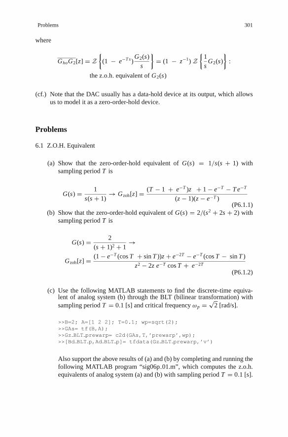
Problems 301
where
GhoG2[z] = Z{
(1 − e−T s)G2(s)
s
}= (1 − z−1) Z
{1
sG2(s)
}:
the z.o.h. equivalent of G2(s)
(cf.) Note that the DAC usually has a data-hold device at its output, which allowsus to model it as a zero-order-hold device.
Problems
6.1 Z.O.H. Equivalent
(a) Show that the zero-order-hold equivalent of G(s) = 1/s(s + 1) withsampling period T is
G(s) = 1
s(s + 1)→ Gzoh[z] = (T − 1 + e−T )z + 1 − e−T − T e−T
(z − 1)(z − e−T )(P6.1.1)
(b) Show that the zero-order-hold equivalent of G(s) = 2/(s2 + 2s + 2) withsampling period T is
G(s) = 2
(s + 1)2 + 1→
Gzoh[z] = (1 − e−T (cos T + sin T ))z + e−2T − e−T (cos T − sin T )
z2 − 2z e−T cos T + e−2T
(P6.1.2)
(c) Use the following MATLAB statements to find the discrete-time equiva-lent of analog system (b) through the BLT (bilinear transformation) withsampling period T = 0.1 [s] and critical frequency ωp = √
2 [rad/s].
>>B=2; A=[1 2 2]; T=0.1; wp=sqrt(2);>>GAs= tf(B,A);>>Gz BLT prewarp= c2d(GAs,T,’prewarp’,wp);>>[Bd BLT p,Ad BLT p]= tfdata(Gz BLT prewarp,’v’)
Also support the above results of (a) and (b) by completing and running thefollowing MATLAB program “sig06p 01.m”, which computes the z.o.h.equivalents of analog system (a) and (b) with sampling period T = 0.1 [s].

302 6 Continuous-Time Systems and Discrete-Time Systems
%sig06p 01.mclear, clfB=1; A=[1 1 0]; T=0.1; e T= exp(-T); e 2T= exp(-2*T);GAs= tf(B,A); % Analog transfer functionGz zoh= c2d(GAs,T); % z.o.h. equivalent[Bd zoh,Ad zoh]= tfdata(Gz zoh,’v’)Bd= [(T-1+e T) 1-e T-T*e T], Ad= [1 -1-e T e T] % (P6.1.1)
(d) Referring to the Simulink block diagram of Fig. P6.1, perform the Simulinksimulation to obtain the step responses of the analog system (b) and its twodiscrete-time equivalents, one through z.o.h. and one through BLT.
Ad_zoh(z)
Bd_zoh(z)
Transfer Fcn
Discrete Filter 1
[Simulink/Discrete][Simulink/Sources]Step
[Simulink/Sinks]Scope
[Simulink/Continuous]
Discrete Filter
2s2 + 2s + 2
Ad_BLT_p(z)
Bd_BLT_p(z)
Fig. P6.1 Simulink block diagram for Problem 6.1
X (s ) Y (s )
G1(s ) G2(s )x (t ) y (t )1
s + 12
s + 2
Fig. P6.2
6.2 Step-Invariant TransformationConsider the system depicted in Fig. P6.2.
(a) Find the step-invariant equivalent G1[z] of G1(s).(b) Find the step-invariant equivalent G2[z] of G2(s).(c) Find the step-invariant equivalent G[z] of G1(s)G2(s).(d) Is it true that G[z] = G1[z]G2[z]?
6.3 Bilinear Transformation without prewarping or with prewarpingConsider the second-order analog system whose transfer function is

Problems 303
G A(s) = ωbs
s2 + ωbs + ω2p
= 2s
s2 + 2s + 1with ωb = 2, ωp = 1 (P6.3.1)
Note that the frequency response G A( jω), its peak frequency, and two 3dB-frequencies are
G A( jω) = jωωb
( jω)2 + jωωb + ω2p
= j2ω
(1 − ω2) + j2ω(P6.3.2)
ωp = 1, ω3B,l =−ωb +
√ω2
b + 4ω2p
2= −1 +
√2,
ω3B,u =ωb +
√ω2
b + 4ω2p
2= 1 +
√2 (P6.3.3)
(a) Find the discrete-time equivalent G D[z] using the BLT with samplingperiod of T = 1 [s] and no prewarping. Also find the peak frequency Ωp
and lower/upper 3dB frequencies Ω3B,l and Ω3B,u of the digital frequencyresponse G D[e jΩ]. How are they related with ωp, ω3B,l , and ω3B,u? Youcan modify and use the MATLAB program “sig06p 03.m” below.
(b) Find the discrete-time equivalent G D[z] using the BLT with samplingperiod of T = 1 [s] and prewarping three times, once at ωp = 1, once atω3B,l , and once at ω3B,u . Also for each G D[z], find the peak frequency Ωp
and lower/upper 3dB frequencies Ω3B,l and Ω3B,u of the digital frequencyresponse G D[e jΩ] and tell which frequency is closest to the correspondinganalog frequency in terms of the basic realtionship Ω = ωT between theanalog and digital frequencies.
%sig06p 03.mB=[2 0]; A=[1 2 1]; wp=1; w 3dB1= -1+sqrt(2); w 3dB2= 1+sqrt(2);GAs= tf(B,A); T=1; % Analog transfer function and sampling periodGz= c2d(GAs,T,’tustin’); % BLT without prewarpingW=[0:0.00001:1]*pi; GDW mag= abs(freqz(BD,AD,W));[GDW max,i peak]= max(GDW mag); Wp= W(i peak)tmp= abs(GDW mag-GDW max/sqrt(2));[tmp 3dB1,i 3dB1]= min(tmp(1:i peak));[tmp 3dB2,i 3dB2]= min(tmp(i peak+1:end));W 3dB1= W(i 3dB1); W 3dB2= W(i peak+i 3dB2);
6.4 Pole Locations and Time ResponsesConsider an analog system having the system function Ga(s) = 1/(s2 +2s +5)and its two z.o.h. equivalents Gzoh1[z] and Gzoh2[z], each with sampling periodT = 0.2 and T = 0.1, respectively.

304 6 Continuous-Time Systems and Discrete-Time Systems
× 1
× 1
–2 –1 102
2
1
–1
–2
s–plane
z–plane
Re{s}
lm{s}
Re{z}
lm{z}
×2
××
××
2
–1 0
–1
–0.5
3
0.5–0.5
0.5
(a) The pole/zero plot of Ga(s) (b) The pole/zero plot of Gzoh1[z] and Gzoh2[z]
(c) The Simulink model window
(d) The Scope window showing the simulation results
3
Fig. P6.4 Pole/zero plots and Simulink simulation

Problems 305
(a) Note that the pole-zero plot of Ga(s) is depicted in Fig. P6.4(a). Refer-ring to the pole/zero plots shown in Fig. P6.4(b), choose the pole locations(r∠Ω) of Gzoh1[z] and Gzoh2[z] from 2© and 3©. The digital frequency ωnTof the output corresponding to pole location 2© is expected to be two timesas high as that of the output corresponding to pole location 3© in proportionto the sampling period T where ωn is determined from the pole location ofthe analog system Ga(s). Does it mean that the output corresponding topole location 2© oscillates two times as fast as that corresponding to polelocation 3©?
(b) Referring to Fig. P6.4(c), perform the Simulink simulation for Ga(s),Gzoh1[z], and Gzoh2[z] to get the simulation results as Fig. P6.4(d) andchoose the output waveforms of Ga(s), Gzoh1[z] and Gzoh2[z] from 1©, 2©,and 3©.
×1
–2 –1 1
2
2
1
–1
–2
s–plane
z–plane
Re{s}
lm{s}
Re{z}
lm{z}
–1 0
–1
4
(a) The pole/zero plot of Ga1(s) and Ga2(s) (b) The pole/zero plot of Gzoh1[z ] and Gzoh2[z ]
×2
×2
×1
34
3×
×× ××
×
(c) The Simulink model window and the simulation results seen in the Scope window
Fig. P6.5 Pole/zero plots and Simulink simulation
6.5 Pole Locations and Time ResponsesConsider two analog systems, each having the system function G1(s) = 1/(s2+2s + 5) and G2(s) = 1/(s2 + 0.4s + 4.04), respectively and their z.o.h.equivalents Gzoh1[z] and Gzoh2[z] with sampling period T = 0.1.

306 6 Continuous-Time Systems and Discrete-Time Systems
(a) Note that the pole-zero plots of G1(s) and G2(s) are depicted in Fig. P6.5(a).Referring to the pole/zero plots shown in Fig. P6.5(b), choose the pole loca-tions of Gzoh1[z] and Gzoh2[z] from 3© and 4©. Which converges faster ofthe outputs stemming from the poles 3© and 4©? Note that the poles 3© arecloser to the origin than the poles 4©, i.e., r3 < r4.
(b) Referring to Fig. P6.5(c), perform the Simulink simulation for G1(s), G2(s),Gzoh1[z], and Gzoh2[z] and choose the output waveforms of the four systemsfrom a©, b©, c©, and d©.
6.6 Pole-Zero Mapping (Matched z-Transform) of an Analog System with DelayUsing the pole-zero mapping (matched z-transform), find the discrete-timeequivalent of an analog system
G(s) = 2
s + 2e−0.95s (P6.6.1)
with sampling period T = 1/4 [s].

Chapter 7Analog and Digital Filters
Contents
7.1 Analog Filter Design . . . . . . . . . . . . . . . . . . . . . . . . . . . . . . . . . . . . . . . . . . . . . . . . . . . . . . . 3077.2 Digital Filter Design . . . . . . . . . . . . . . . . . . . . . . . . . . . . . . . . . . . . . . . . . . . . . . . . . . . . . . . . 320
7.2.1 IIR Filter Design . . . . . . . . . . . . . . . . . . . . . . . . . . . . . . . . . . . . . . . . . . . . . . . . . . . 3217.2.2 FIR Filter Design . . . . . . . . . . . . . . . . . . . . . . . . . . . . . . . . . . . . . . . . . . . . . . . . . . . 3317.2.3 Filter Structure and System Model Available in MATLAB . . . . . . . . . . . . . . . . . 3457.2.4 Importing/Exporting a Filter Design . . . . . . . . . . . . . . . . . . . . . . . . . . . . . . . . . . . 348
7.3 How to Use SPTool . . . . . . . . . . . . . . . . . . . . . . . . . . . . . . . . . . . . . . . . . . . . . . . . . . . . . . . . 350Problems . . . . . . . . . . . . . . . . . . . . . . . . . . . . . . . . . . . . . . . . . . . . . . . . . . . . . . . . . . . . . . . . . 357
This chapter introduces how to use MATLAB for designing analog and digitalfilters such that the given specification on the frequency response is satisfied. Espe-cially for analog filters, the MATLAB routines to perform circuit-level design arealso introduced.
7.1 Analog Filter Design
This section has been excerpted from Sect. 8.6 of [Y-2] (Yang, Won Y. and SeungC. Lee, Circuit Systems with MATLAB and PSpice, John Wiley & Sons, Inc., NewJersey, 2007.). Fig 7.1(a)/(b)/(c)/(d) show typical lowpass/bandpass/bandstop/ high-pass filter specifications on their log-magnitude, 20 log10 |G( jω)| [dB], of frequencyresponse. The filter specification can be described as follows:
20 log10 |G( jωp)| ≥ −Rp[dB] for the passband (7.1.1a)
20 log10 |G( jωs)| ≤ −As[dB] for the stopband (7.1.1b)
where ωp, ωs , Rp, and As are referred to as the passband edge frequency, thestopband edge frequency, the passband ripple, and the stopband attenuation, respec-tively. The most commonly used analog filter design techniques are the Butterworth,Chebyshev I, II, and elliptic ones ([K-2], Chap. 8). MATLAB has the built-infunctions butt(), cheby1(), cheby2(), and ellip() for designing thefour types of analog/digital filter. As summarized below, butt() needs the 3dBcutoff frequency while cheby1() and ellip() get the critical passband edge
W.Y. Yang et al., Signals and Systems with MATLAB R©,DOI 10.1007/978-3-540-92954-3 7, C© Springer-Verlag Berlin Heidelberg 2009
307
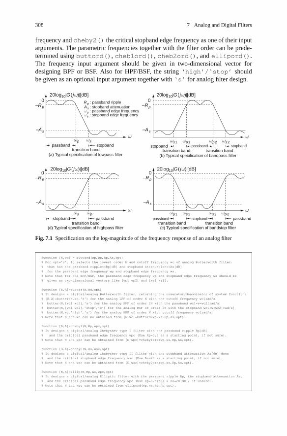
308 7 Analog and Digital Filters
frequency and cheby2() the critical stopband edge frequency as one of their inputarguments. The parametric frequencies together with the filter order can be prede-termined using buttord(), cheb1ord(), cheb2ord(), and ellipord().The frequency input argument should be given in two-dimensional vector fordesigning BPF or BSF. Also for HPF/BSF, the string ‘high’/‘stop’ shouldbe given as an optional input argument together with ‘s’ for analog filter design.
20log10|G ( jω)|[dB]
(a) Typical specification of lowpass filter (b) Typical specification of bandpass filter
(d) Typical specification of highpass filtertransition band
transition bandpassband
passbandpassband
passband stopband
stopband passband
stopbandstopband
stopband
transition band transition band
transition band transition band(c) Typical specification of bandstop filter
0–Rp
Rp : passband rippleAs : stopband attenuationωp : passband edge frequencyω s : stopband edge frequency
–As
0–Rp
–As
0–Rp
–As
0–Rp
–As
20log10|G ( jω)|[dB] 20log10|G ( jω)|[dB]
20log10|G ( jω)|[dB]
ω
ω ω
ωωs2ωp2ωp1ωs1
ωp1 ωs1 ωs2 ωp2
ωsωp
ωs ωp
Fig. 7.1 Specification on the log-magnitude of the frequency response of an analog filter
function [N,wc] = buttord(wp,ws,Rp,As,opt)
% For opt=’s’, it selects the lowest order N and cutoff frequency wc of analog Butterworth filter.
% that has the passband ripple<=Rp[dB] and stopband attenuation>=As[dB]
% for the passband edge frequency wp and stopband edge frequency ws.
% Note that for the BPF/BSF, the passband edge frequency wp and stopband edge frequency ws should be
% given as two-dimensional vectors like [wp1 wp2] and [ws1 ws2].
function [B,A]=butter(N,wc,opt)
% It designs a digital/analog Butterworth filter, returning the numerator/denominator of system function.
% [B,A]=butter(N,wc,’s’) for the analog LPF of order N with the cutoff frequency wc[rad/s]
% butter(N,[wc1 wc2],’s’) for the analog BPF of order 2N with the passband wc1<w<wc2[rad/s]
% butter(N,[wc1 wc2],’stop’,’s’) for the analog BSF of order 2N with the stopband wc1<w<wc2[rad/s]
% butter(N,wc,’high’,’s’) for the analog HPF of order N with cutoff frequency wc[rad/s]
% Note that N and wc can be obtained from [N,wc]=buttord(wp,ws,Rp,As,opt).
function [B,A]=cheby1(N,Rp,wpc,opt)
% It designs a digital/analog Chebyshev type I filter with the passband ripple Rp[dB]
% and the critical passband edge frequency wpc (Use Rp=0.5 as a starting point, if not sure).
% Note that N and wpc can be obtained from [N,wpc]=cheby1ord(wp,ws,Rp,As,opt).
function [B,A]=cheby2(N,As,wsc,opt)
% It designs a digital/analog Chebyshev type II filter with the stopband attenuation As[dB] down
% and the critical stopband edge frequency wsc (Use As=20 as a starting point, if not sure).
% Note that N and wsc can be obtained from [N,wsc]=cheby2ord(wp,ws,Rp,As,opt).
function [B,A]=ellip(N,Rp,As,wpc,opt)
% It designs a digital/analog Elliptic filter with the passband ripple Rp, the stopband attenuation As,
% and the critical passband edge frequency wpc (Use Rp=0.5[dB] & As=20[dB], if unsure).
% Note that N and wpc can be obtained from ellipord(wp,ws,Rp,As,opt).

7.1 Analog Filter Design 309
G0(s)
G0(s)
G1(s)
summer
(a) Cascade form (b) Parallel form
G2(s)
GM(s)
G1(s) G2(s) GM (s)
G0(s)+ Gm(s)G (s) ΣMm=1=
G (s) G0(s) Gm(s)MΠ
m=1
Vo (s)
Vi (s)= =
Fig. 7.2 Two realizations of an analog filter (system or transfer function)
The designed filter system functions are often factored into the sum or product ofsecond-order sections called biquads (possibly with an additional first-order sectionin the case of an odd filter order) as
G(s) =K G0(s)MΠ
m=1Gm(s) = K
b01s + b02
s + a02
MΠ
m=1
bm1s2 + bm2s + bm3
s2 + am2s + am3(7.1.2a)
with M = floor(
N2
)
G(s) =G0(s) +∑M
m=1Gm(s) = b01s + b02
s + a02+∑M
m=1
bm1s2 + bm2s + bm3
s2 + am2s + am3(7.1.2b)
with M = floor
(N
2
)
and then realized in cascade or parallel form, respectively as depicted in Fig. 7.2.Rather than reviewing the design procedures, let us use the MATLAB functions
to design a Butterworth lowpass filter, a Chebyshev I bandpass filter, a ChebyshevII bandstop filter, and elliptic highpass filter in the following example.
Example 7.1 Analog Filter Design Using the MATLAB FunctionsLet us find the system functions of analog filters meeting the specifications
given below.
(a)We are going to determine the system function of a Butterworth lowpass filter with
ωp = 2π × 6000 [rad/s], ωs = 2π × 15000 [rad/s], Rp = 2 [dB], and
As = 25 [dB] (E7.1.1)
First, we use the MATLAB function ‘buttord()’ to find the filter order N andthe cutoff frequency ωc at which 20 log10 |G( jωc)| = −3 [dB] by typing thefollowing statements into the MATLAB command window:

310 7 Analog and Digital Filters
>>wp=2*pi*6000; ws=2*pi*15000; Rp=2; As=25;>>format short e, [N,wc]=buttord(wp,ws,Rp,As,’s’)
N = 4, wc = 4.5914e+004
We put these parameter values N and wc into the Butterworth filter design func-tion ‘butter()’ as its first and second input arguments:
>>[Bb,Ab]=butter(N,wc,’s’)
Bb = 0 0 0 0 4.4440e+018
Ab = 1.0000e+000 1.1998e+005 7.1974e+009 2.5292e+014 4.4440e+018
This means that the system function of the designed Butterworth LPF of orderN=4 is
G(s) = 4.444 × 10¹⁸
s4 + 1.1998 × 10⁵s3 + 7.1974 × 10⁹s2 + 2.5292 × 10¹⁴s + 4.444 × 10¹⁸
(E7.1.2)
We can find the cascade and parallel realizations of this system function by typingthe following statements into the MATLAB command window:
>>[SOS,K]=tf2sos(Bb,Ab); % cascade realization>>Ns=size(SOS,1); >>Gm=Kˆ(1/Ns), BBc=SOS(:,1:3), AAc=SOS(:,4:6)
Gm = 2.1081e+009BBc = 0 0 1 AAc = 1.0000e+000 3.5141e+004 2.1081e+009
0 0 1 1.0000e+000 8.4838e+004 2.1081e+009>>[BBp,AAp]=tf2par s(Bb,Ab) % parallel realization (see Sect. E.15)
BBp = 0 4.2419e+004 3.5987e+0090 -4.2419e+004 -1.4906e+009
AAp = 1.0000e+000 8.4838e+004 2.1081e+0091.0000e+000 3.5141e+004 2.1081e+009
This means that the designed system function can be realized in cascade andparallel form as
G(s) = 2.108 × 10⁹
s2 + 3.514 × 10⁴s + 2.108 × 109× 2.108 × 109
s2 + 8.484 × 10⁴s + 2.108 × 10⁹
(E7.1.3a)
G(s) = 4.242 × 10⁴s + 3.599 × 10⁹
s2 + 8.484 × 10⁴s + 2.108 × 10⁹− 4.242 × 10⁴s + 1.491 × 10⁹
s2 + 3.514 × 10⁴s + 2.108 × 10⁹
(E7.1.3b)
(b)We are going to determine the system function of a Chebyshev I bandpass fil-ter with
ωs1 = 2π × 6000, ωp1 = 2π × 10000, ωp2 = 2π × 12000,
ωs2 = 2π × 15000 [rad/s], Rp = 2 [dB], and As = 25 [dB] (E7.1.4)
First, we use the MATLAB function ‘cheb1ord()’ to find the filter order N andthe critical passband edge frequencies ωpc1 and ωpc2 at which the passband rip-ple condition is closely met, i.e., 20 log10 |G( jωpc)| = −Rp [dB] by typing thefollowing statements:
7.1 Analog Filter Design 311
>>ws1=2*pi*6e3; wp1=2*pi*1e4; wp2=2*pi*12e3; ws2=2*pi*15e3; Rp=2; As=25;>>[N,wpc]=cheb1ord([wp1 wp2],[ws1 ws2],Rp,As,’s’)
N = 2, wpc = 6.2832e+004 7.5398e+004
We put the (half) filter order N, the passband ripple Rp, and the critical passbandedge frequency vector wpc = [ωpc1 ωpc2] into the Chebyshev I filter designfunction ‘cheby1()’ as>>[Bc1,Ac1]=cheby1(N,Rp,wpc,’s’)
Bc1 = 0 0 1.0324e+008 0 0Ac1 = 1.0000e+000 1.0101e+004 9.6048e+009 4.7853e+013 2.2443e+019
This means that the system function of the designed Chebyshev I BPF of order2N=4 is
G(s) = 1.0324 × 10⁸s2
s4 + 10101s3 + 9.6048 × 10⁹s2 + 4.7853 × 10¹³s + 2.2443 × 10¹⁹
(E7.1.5)
We can find the cascade and parallel realizations of this system function by typingthe following statements into the MATLAB command window:
>>[SOS,K]=tf2sos(Bc1,Ac1); % cascade realization>>Ns=size(SOS,1); Gm=Kˆ(1/Ns), BBc=SOS(:,1:3), AAc=SOS(:,4:6)
Gm = 1.0161e+004BBc = 0 0 1 AAc = 1.0000e+000 5.4247e+003 5.4956e+009
1 0 1 1.0000e+000 4.6763e+003 4.0838e+009>>[BBp,AAp]=tf2par s(Bc1,Ac1) % parallel realization
BBp = 0 1.8390e+002 4.0242e+0080 -1.8390e+002 -2.9904e+008
AAp = 1.0000e+000 5.4247e+003 5.4956e+0091.0000e+000 4.6763e+003 4.0838e+009
This means that the designed system function can be realized in cascade andparallel form as
G(s) = 1.0161 × 10⁴s
s2 + 5.425 × 10³s + 5.496 × 109× 1.0161 × 104s
s2 + 4.676 × 10³s + 4.084 × 10⁹
(E7.1.6a)
G(s) = 1.839 × 10²s + 4.024 × 10⁸
s2 + 5.425 × 10³s + 5.496 × 10⁹− 1.839 × 10²s + 2.990 × 10⁸
s2 + 4.676 × 10³s + 4.084 × 10⁹
(E7.1.6b)
(c)We are going to determine the system function of a Chebyshev II bandstopfilter with
ωp1 = 2π × 6000, ωs1 = 2π × 10000, ωs2 = 2π × 12000,
ωp2 = 2π × 15000 [rad/s], Rp = 2 [dB], and As = 25 [dB] (E7.1.7)
First, we use the MATLAB function ‘cheb2ord()’ to find the filter order N andthe critical stopband edge frequencies ωsc1 and ωsc2 at which the stopband atten-uation condition is closely met, i.e., 20 log10 |G( jωsc)| = −As [dB] by typingthe following statements:

312 7 Analog and Digital Filters
>>wp1=2*pi*6000; ws1=2*pi*10000; ws2=2*pi*12000; wp2=2*pi*15000;
>>Rp=2; As=25;
>>[N,wsc]=cheb2ord([wp1 wp2],[ws1 ws2],Rp,As,’s’)
N = 2, wsc = 6.2798e+004 7.5438e+004
We put the (half) filter order N, the stopband attenuation As, and the criticalstopband edge frequency vector wsc = [ωsc1 ωsc2] into the Chebyshev II filterdesign function ‘cheby2()’ as
>>[Bc2,Ac2]=cheby2(N,As,wsc,’stop’,’s’)Bc2 = 1.0000e+000 1.0979e-010 9.5547e+009 4.9629e-001 2.2443e+019Ac2 = 1.0000e+000 5.1782e+004 1.0895e+010 2.4531e+014 2.2443e+019
This means that the system function of the designed Chebyshev II BSF of order2N = 4 is
G(s) = s4 + 9.5547 × 10⁹s2 + 4.9629 × 10⁻¹s + 2.2443 × 10¹⁹
s4 + 51782s3 + 1.0895 × 10¹⁰s2 + 2.4531 × 10¹⁴s + 2.2443 × 10¹⁹
(E7.1.8)
We can find the cascade and parallel realizations of this system function by typingthe following statements into the MATLAB command window:
>>[SOS,K]=tf2sos(Bc2,Ac2); % cascade realization [BBc,AAc]=tf2cas(B,A)>>Ns=size(SOS,1); Gm=Kˆ(1/Ns), BBc=SOS(:,1:3), AAc=SOS(:,4:6)
Gm = 1BBc = 1.0000e+000 7.7795e-011 5.3938e+009
1.0000e+000 2.9104e-011 4.1609e+009AAc = 1.0000e+000 3.1028e+004 7.0828e+009
1.0000e+000 2.0754e+004 3.1687e+009>>[BBp,AAp]=tf2par s(Bc2,Ac2) % parallel realization
BBp = 5.0000e-001 -1.5688e+004 3.4426e+0095.0000e-001 -1.0204e+004 1.6285e+009
AAp = 1.0000e+000 3.1028e+004 7.0828e+0091.0000e+000 2.0754e+004 3.1687e+009
This means that the designed system function can be realized in cascade andparallel form as
G(s) = s2 + 5.394 × 10⁹
s2 + 3.103 × 10⁴s + 7.083 × 10⁹× s2 + 4.161 × 10⁹
s2 + 2.075 × 10⁴s + 3.169 × 10⁹
(E7.1.9a)
G(s) = 0.5s2 − 1.569 × 10⁴s + 3.443 × 10⁹
s2 + 3.103 × 10⁴s + 7.083 × 10⁹+ 0.5s2 − 1.020 × 10⁴s + 1.6285 × 10⁹
s2 + 2.075 × 10⁴s + 3.169 × 10⁹
(E7.1.9b)
(d)We are going to determine the system function of an elliptic highpass filter with
ωs = 2π × 6000 [rad/s], ωp = 2π × 15000 [rad/s], Rp = 2 [dB], and As = 25 [dB](E7.1.10)
First, we use the MATLAB function ‘ellipord()’ to find the filter order N and thecritical passband edge frequency ωpc at which 20 log10 |G( jωpc)| = −Rp [dB]by typing the following statements into the MATLAB command window:

7.1 Analog Filter Design 313
>>ws=2*pi*6000; wp=2*pi*15000; Rp=2; As=25;>>format short e, [N,wc]=ellipord(wp,ws,Rp,As,’s’)
N = 3, wc = 9.4248e+004
We put the parameter values N, Rp, As, and wc into the elliptic filter designfunction ‘ellip()’ as
>>[Be,Ae]=ellip(N,Rp,As,wc,’high’,’s’)Be = 1.0000e+000 8.9574e-009 3.9429e+009 -5.6429e+002Ae = 1.0000e+000 2.3303e+005 1.4972e+010 1.9511e+015
This means that the system function of the designed elliptic HPF of order N =3 is
G(s) = s3 + 3.9429 × 10⁹s − 5.6429 × 10²
s3 + 2.3303 × 10⁵s2 + 1.4972 × 10¹⁰s + 1.9511 × 10¹⁵(E7.1.11)
We can find the cascade and parallel realizations of this system function by typingthe following statements into the MATLAB command window:
>>[SOS,K]=tf2sos(Be,Ae); % cascade realization>>Ns=size(SOS,1); Gm=Kˆ(1/Ns), BBc=SOS(:,1:3), AAc=SOS(:,4:6)
Gm = 1.0000e+000BBc = 1.0000e+000 -1.4311e-007 0
1.0000e+000 1.5207e-007 3.9429e+009AAc = 1.0000e+000 2.0630e+005 0
1.0000e+000 2.6731e+004 9.4575e+009>>[BBp,AAp]=tf2par s(Be,Ae) % parallel realization
BBp = 5.0000e-001 -1.3365e+004 4.7287e+0090 5.0000e-001 -1.0315e+005
AAp = 1.0000e+000 2.6731e+004 9.4575e+0090 1.0000e+000 2.0630e+005
This means that the designed system function can be realized in cascade andparallel form as
G(s) = s
s + 2.063 × 10⁵× s2 + 3.943 × 10⁹
s2 + 2.673 × 10⁴s + 9.458 × 10⁹(E7.1.12a)
G(s) = 0.5s2 − 1.337 × 10⁴s + 4.729 × 10⁹
s2 + 2.673 × 10⁴s + 9.458 × 10⁹+ 0.5s − 1.032 × 10⁵
s + 2.063 × 10⁵
(E7.1.12b)
(e)All the above filter design works are put into the M-file named “sig07e01.m”,which plots the frequency responses of the designed filters so that one can checkif the design specifications are satisfied. Figure 7.3, obtained by running theprogram “sig07e01.m”, shows the following points:
- Figure 7.3(a) shows that the cutoff frequency ωc given as an input argument of‘butter()’ is the frequency at which 20 log10 |G( jωc)| = −3 [dB]. Note that thefrequency response magnitude of a Butterworth filter is monotonic, i.e., has noripple.
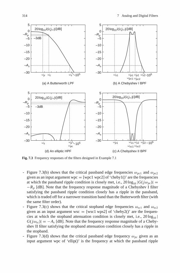
314 7 Analog and Digital Filters
20log10 G ( jω) [dB]
20log10 G ( jω) [dB] 20log10 G ( jω) [dB]
20log10 G ( jω) [dB]
ωs2
5
0
–5 –3dB
–3dB
–10
–15
–20
–30
(a) A Butterworth LPF (b) A Chebyshev I BPF
(c) A Chebyshev II BPF(d) An elliptic HPF
105
105 105
105ωp
ωs ωpωpc
ωs1 ωp1
ωp1 ωs1ωsc1 ωsc2
ωs2 ωp2
ωpc1 ωpc2
ωp2ωc ωs
–As
–Rp
5
0
–5
–10
–15
–20
–30
–As
–Rp
5
0
–5
–10
–15
–20
–30
–As
–Rp
5
0
–5
–10
–15
–20
–30
–As
–Rp
Fig. 7.3 Frequency responses of the filters designed in Example 7.1
- Figure 7.3(b) shows that the critical passband edge frequencies ωpc1 and ωpc2
given as an input argument wpc = [wpc1 wpc2] of ‘cheby1()’ are the frequenciesat which the passband ripple condition is closely met, i.e., 20 log10 |G( jωpc)| =−Rp [dB]. Note that the frequency response magnitude of a Chebyshev I filtersatisfying the passband ripple condition closely has a ripple in the passband,which is traded off for a narrower transition band than the Butterworth filter (withthe same filter order).
- Figure 7.3(c) shows that the critical stopband edge frequencies ωsc1 and ωsc2
given as an input argument wsc = [wsc1 wps2] of ‘cheby2()’ are the frequen-cies at which the stopband attenuation condition is closely met, i.e., 20 log10 |G( jωsc)| = −As [dB]. Note that the frequency response magnitude of a Cheby-shev II filter satisfying the stopband attenuation condition closely has a ripple inthe stopband.
- Figure 7.3(d) shows that the critical passband edge frequency ωpc given as aninput argument wpc of ‘ellip()’ is the frequency at which the passband ripple

7.1 Analog Filter Design 315
condition is closely met, i.e., 20 log10 |G( jωpc)| = −Rp [dB]. Note that the fre-quency response magnitude of an elliptic filter has ripples in both the passbandand the stopband, yielding a relatively narrow transition band with the smallestfilter order N = 3 among the four filters.
%sig07e01.m for analog filter design and frequency response plotclear, clf, format short edisp(’(a) Butterworth LPF’)wp=2*pi*6000; ws=2*pi*15000; Rp=2; As=25;[Nb,wcb]= buttord(wp,ws,Rp,As,’s’) % Order of analog BW LPF[Bb,Ab]= butter(Nb,wcb,’s’) % num/den of analog BW LPF system ftn[SOS,K]= tf2sos(Bb,Ab); % cascade realization [BBc,AAc]=tf2cas(B,A)Ns=size(SOS,1); Gm=Kˆ(1/Ns), BBc=SOS(:,1:3), AAc=SOS(:,4:6)[BBp,AAp]= tf2par s(Bb,Ab) % parallel realization -- see Sect. E.15ww= logspace(4,6,1000); % log frequency vector from 1e4 to 1e6[rad/s]subplot(221), semilogx(ww,20*log10(abs(freqs(Bb,Ab,ww))))title(’Butterworth LPF’)
disp(’(b) Chebyshev I BPF’)ws1=2*pi*6e3; wp1=2*pi*1e4; wp2=2*pi*12e3; ws2=2*pi*15e3; Rp=2; As=25;[Nc1,wpc]= cheb1ord([wp1 wp2],[ws1 ws2],Rp,As,’s’)[Bc1,Ac1]= cheby1(Nc1,Rp,wpc,’s’)[SOS,K]= tf2sos(Bc1,Ac1); % cascade realizationNs=size(SOS,1); Gm=Kˆ(1/Ns), BBc=SOS(:,1:3), AAc=SOS(:,4:6)[BBp,AAp]= tf2par s(Bc1,Ac1) % parallel realizationsubplot(222), semilogx(ww,20*log10(abs(freqs(Bc1,Ac1,ww))))title(’Chebyshev I BPF’)
disp(’(c) Chebyshev II BSF’)wp1=2*pi*6e3; ws1=2*pi*1e4; ws2=2*pi*12e3; wp2=2*pi*15e3; Rp=2; As=25;[Nc2,wsc]= cheb2ord([wp1 wp2],[ws1 ws2],Rp,As,’s’)[Bc2,Ac2]= cheby2(Nc2,As,wsc,’stop’,’s’)[SOS,K]= tf2sos(Bc2,Ac2); % cascade realizationNs=size(SOS,1); Gm=Kˆ(1/Ns), BBc=SOS(:,1:3), AAc=SOS(:,4:6)[BBp,AAp]= tf2par s(Bc2,Ac2) % parallel realizationsubplot(224), semilogx(ww,20*log10(abs(freqs(Bc2,Ac2,ww))))title(’Chebyshev II BSF’)disp(’(d) Elliptic HPF’)
ws=2*pi*6000; wp=2*pi*15000; Rp=2; As=25;[Ne,wpc]= ellipord(wp,ws,Rp,As,’s’)[Be,Ae]= ellip(Ne,Rp,As,wpc,’high’,’s’)[SOS,K]= tf2sos(Be,Ae); % cascade realizationNs=size(SOS,1); Gm=Kˆ(1/Ns), BBc=SOS(:,1:3), AAc=SOS(:,4:6)[BBp,AAp]= tf2par s(Be,Ae) % parallel realizationsubplot(223), semilogx(ww,20*log10(abs(freqs(Be,Ae,ww))))
Now we are going to conclude this section with some MATLAB routines thatcan be used to determine the parameters of the circuits depicted in Figs. 7.4, 7.5,and 7.6 so that they can realize the designed (second-order) system functions. SeeChap. 8 of [Y-2] for more details.
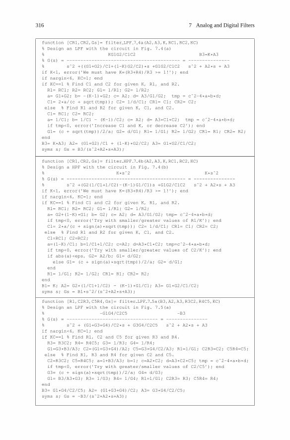
316 7 Analog and Digital Filters
function [CR1,CR2,Gs]= filter LPF 7 4a(A2,A3,K,RC1,RC2,KC)% Design an LPF with the circuit in Fig. 7.4(a)% KG1G2/C1C2 B3=K*A3% G(s) = ----------------------------------------- = ---------------% sˆ2 +((G1+G2)/C1+(1-K)G2/C2)*s +G1G2/C1C2 sˆ2 + A2*s + A3if K<1, error(’We must have K=(R3+R4)/R3 >= 1!’); endif nargin<6, KC=1; endif KC==1 % Find C1 and C2 for given K, R1, and R2.R1= RC1; R2= RC2; G1= 1/R1; G2= 1/R2;a= G1+G2; b= -(K-1)*G2; c= A2; d= A3/G1/G2; tmp = cˆ2-4*a*b*d;C1= 2*a/(c + sqrt(tmp)); C2= 1/d/C1; CR1= C1; CR2= C2;else % Find R1 and R2 for given K, C1, and C2.C1= RC1; C2= RC2;a= 1/C1; b= 1/C1 - (K-1)/C2; c= A2; d= A3*C1*C2; tmp = cˆ2-4*a*b*d;if tmp<0, error(’Increase C1 and K, or decrease C2’); endG1= (c + sqrt(tmp))/2/a; G2= d/G1; R1= 1/G1; R2= 1/G2; CR1= R1; CR2= R2;
endB3= K*A3; A2= (G1+G2)/C1 + (1-K)*G2/C2; A3= G1*G2/C1/C2;syms s; Gs = B3/(sˆ2+A2*s+A3);
function [CR1,CR2,Gs]= filter HPF 7 4b(A2,A3,K,RC1,RC2,KC)% Design a HPF with the circuit in Fig. 7.4(b)% K*sˆ2 K*sˆ2% G(s) = ------------------------------------------- = ---------------% sˆ2 +(G2(1/C1+1/C2)-(K-1)G1/C1)s +G1G2/C1C2 sˆ2 + A2*s + A3if K<1, error(’We must have K=(R3+R4)/R3 >= 1!’); endif nargin<6, KC=1; endif KC==1 % Find C1 and C2 for given K, R1, and R2.R1= RC1; R2= RC2; G1= 1/R1; G2= 1/R2;a= G2+(1-K)*G1; b= G2; c= A2; d= A3/G1/G2; tmp= cˆ2-4*a*b*d;if tmp<0, error(’Try with smaller/greater values of R1/K’); endC1= 2*a/(c + sign(a)*sqrt(tmp)); C2= 1/d/C1; CR1= C1; CR2= C2;
else % Find R1 and R2 for given K, C1, and C2.C1=RC1; C2=RC2;a=(1-K)/C1; b=1/C1+1/C2; c=A2; d=A3*C1*C2; tmp=cˆ2-4*a*b*d;if tmp<0, error(’Try with smaller/greater values of C2/K’); endif abs(a)<eps, G2= A2/b; G1= d/G2;else G1= (c + sign(a)*sqrt(tmp))/2/a; G2= d/G1;
endR1= 1/G1; R2= 1/G2; CR1= R1; CR2= R2;
endB1= K; A2= G2*(1/C1+1/C2) - (K-1)*G1/C1; A3= G1*G2/C1/C2;syms s; Gs = B1*sˆ2/(sˆ2+A2*s+A3);
function [R1,C2R3,C5R4,Gs]= filter LPF 7 5a(B3,A2,A3,R3C2,R4C5,KC)% Design an LPF with the circuit in Fig. 7.5(a)% -G1G4/C2C5 -B3% G(s) = --------------------------------- = ---------------% sˆ2 + (G1+G3+G4)/C2*s + G3G4/C2C5 sˆ2 + A2*s + A3if nargin<6, KC=1; endif KC==1 % Find R1, C2 and C5 for given R3 and R4.R3= R3C2; R4= R4C5; G3= 1/R3; G4= 1/R4;G1=G3*B3/A3; C2=(G1+G3+G4)/A2; C5=G3*G4/C2/A3; R1=1/G1; C2R3=C2; C5R4=C5;else % Find R1, R3 and R4 for given C2 and C5.C2=R3C2; C5=R4C5; a=1+B3/A3; b=1; c=A2*C2; d=A3*C2*C5; tmp = cˆ2-4*a*b*d;if tmp<0, error(’Try with greater/smaller values of C2/C5’); endG3= (c + sign(a)*sqrt(tmp))/2/a; G4= d/G3;G1= B3/A3*G3; R3= 1/G3; R4= 1/G4; R1=1/G1; C2R3= R3; C5R4= R4;
endB3= G1*G4/C2/C5; A2= (G1+G3+G4)/C2; A3= G3*G4/C2/C5;syms s; Gs = -B3/(sˆ2+A2*s+A3);

7.1 Analog Filter Design 317
function [C1,C3R2,C4R5,Gs]= filter HPF 7 5b(B1,A2,A3,R2C3,R5C4,KC)% Design a HPF with the circuit in Fig. 7.5(b)% -(C1/C3)*sˆ2 -B1*sˆ2% G(s) = -------------------------------------- = ---------------% sˆ2 + G5(C1+C3+C4)/C3/C4*s + G2G5/C3C4 sˆ2 + A2*s + A3if nargin<6, KC=1; endif KC==1 % Find C1, C3 and C4 for given R2 and R5.R2= R2C3; R5= R5C4; G2= 1/R2; G5= 1/R5;a= 1; b= 1+B1; c= A2/G5; d= A3/G2/G5; tmp = cˆ2-4*a*b*d;if tmp<0, error(’Try with smaller/greater values of R2/R5’); endC3= 2*a/(c + sqrt(tmp)); C4= 1/d/C3; C1= B1*C3; C3R2= C3; C4R5= C4;else % Find C1, R2 and R5 for given C3 and C4.C3= R2C3; C4= R5C4;C1 = B1*C3; G5= A2/(C1+C3+C4)*C3*C4; G2= A3*C3*C4/G5;R2= 1/G2; R5= 1/G5; C3R2= R2; C4R5= R5;
endB1= C1/C3; A2= G5*(C1+C3+C4)/C3/C4; A3= G2*G5/C3/C4;syms s; Gs = -B1*sˆ2/(sˆ2+A2*s+A3);% Examples of Usage%>>B1=2; A2=100; A3=10000;%>> R2=1e4; R5=2e5; [C1,C3,C4,Gs]=filter HPF 7 5b(B1,A2,A3,R2,R5,1)%>> C3=1e-7; C4=2e-6; [C1,R2,R5,Gs]=filter HPF 7 5b(B1,A2,A3,C3,C4,2)
function [C3R1,C4R2,R5,Gs]= filter BPF 7 6a(B2,A2,A3,R1C3,R2C4,KC)% Design a BPF with the circuit in Fig. 7.6(a)% -(G1/C3)*s -B2*s% G(s) = -------------------------------------- = ---------------% sˆ2 + G5(1/C3+1/C4)*s + (G1+G2)G5/C3C4 sˆ2 + A2*s + A3if nargin<6, KC=1; endif KC==1 % Find C3, C4, and R5 for given R1 and R2.R1= R1C3; R2= R2C4; G1= 1/R1; G2= 1/R2; C3= G1/B2;G5= (A2 - A3*C3/(G1+G2))*C3;if G5<0, error(’Try with smaller values of R2’); endC4= G5*(G1+G2)/C3/A3;R5= 1/G5; C3R1= C3; C4R2= C4;fprintf(’C3=%10.4e, C4=%10.4e, R5=%10.4e\n’, C3,C4,R5)elseif KC==2 % Find R1, R2 and R5 for given C3 and C4.C3= R1C3; C4= R2C4;G1 = B2*C3; G5= A2/(1/C3+1/C4); G2= A3*C3*C4/G5-G1;R5= 1/G5; R1=1/G1; R2=1/G2; C3R1= R1; C4R2= R2;fprintf(’R1=%10.4e, R2=%10.4e, R5=%10.4e\n’, R1,R2,R5)else % Find R1, R5, and C3=C4=C for given R2 and C3=C4.R2= R1C3; G2=1/R2;nonlinear eq= inline(’[2*x(1)-A2*x(2); x(1).*(B2*x(2)+G2)-A3*x(2).ˆ2]’,...
’x’,’G2’,’B2’,’A2’,’A3’);G50=0.1; C0=0.1; x0=[G50 C0]; % Initial guesses of G5 and Cx= fsolve(nonlinear eq,x0,optimset(’TolFun’,1e-8),G2,B2,A2,A3)%tol=1e-5; MaxIter=100; x=newtons(nonlinear eq,x0,tol,MaxIter,G2,B2,A2,A3)G5= x(1); C=x(2); C3=C; C4=C; G1=B2*C3;R1=1/G1; R5=1/G5; C3R1=C3; C4R2=R1;fprintf(’C3=C4=%10.4e, R1=%10.4e, R5=%10.4e\n’, C,R1,R5)endB1= G1/C3; A2= G5*(1/C3+1/C4); A3= (G1+G2)*G5/C3/C4;syms s; Gs = -B2*s/(sˆ2+A2*s+A3);% Examples of Usage%>>B2=100; A2=100; A3=10000;%>> R1=1e2; R2=1e2; [C3,C4,R5,Gs]=filter BPF 7 6a(B2,A2,A3,R1,R2,1)%>> C3=1e-4; C4=1e-4; [R1,R2,R5,Gs]=filter BPF 7 6a(B2,A2,A3,C3,C4,2)%>> R2=1e2; [C3,R1,R5,Gs]=filter BPF 7 6a(B2,A2,A3,R2,0,3)

318 7 Analog and Digital Filters
function [C1,C2R3,C5R4,Gs]= filter BPF 7 6b(B2,A2,A3,R3C5,R4C5,KC)% Design a BPF with the circuit in Fig. 7.6(b)% -(C1G4/(C1+C2)C5)*s -B2*s% G(s) = ------------------------------------------ = ---------------% sˆ2 + ((G3+G4)/(C1+C2))*s + G3G4/(C1+C2)C5 sˆ2 + A2*s + A3if nargin<6, KC=1; endif KC==1 % Find C1, C2 and C5 for given R3 and R4.R3= R3C5; R4=R4C5; G3= 1/R3; G4=1/R4;C1pC2= (G3+G4)/A2; C5= G3*G4/A3/C1pC2; C1= B2*C1pC2*C5/G4 %=B2*G3/A3C2= C1pC2 - C1; C2R3= C2; C5R4= C5;if C2<0, error(’Try with greater/smaller values of R3/R4’); endfprintf(’C1=%10.4e, C2=%10.4e, C5=%10.4e\n’, C1,C2,C5)else % Find C1, R3 and R4 for given C5 and C1=C2.C5=R3C5; G4= 2*C5*B2; G3 2C= A3/G4*C5; %=A3/2/B2: not adjustableC= G4/2/(A2-G3 2C); C1=C; C2=C;if C<0, error(’How about increasing B2 & A2 and/or decreasing A3’); endG3= G3 2C*2*C; R3= 1/G3; R4= 1/G4; C2R3= R3; C5R4= R4;fprintf(’C1=C2=%10.4e, R3=%10.4e, R4=%10.4e\n’, C,R3,R4)
endB3= C1*G4/(C1+C2)/C5; A2= (G3+G4)/(C1+C2); A3= G3*G4/(C1+C2)/C5;syms s; Gs = -B2*s/(sˆ2+A2*s+A3);
R3
R2R1
C2
0 0
C1
R4
R3 + R4
R3
U11 P
N
+
–
Vo (s)
K =
Ga (s) = =
Vi(s)VP(s)
VN(s) = VP(s)~ ~
VN(s)
V1(s)
Vo (s)
(a) A second-order Sallen-Key lowpass filter (b) A second-order Sallen-Key highpass filter
KG1G2/C1C2
s2+ ((G1+ G2)/C1+ (1 – K)G2/C2)s + G1G2/C1C2Vi(s)
Gb (s) = =Vo (s)
Vi(s)
R3
C2C1
R2
0 0
R1
R4
R3 + R4
R3
U11 P
N
+
–
Vo (s)
K =
Vi(s)VP(s)
VN(s) = VP(s)VN(s)
V1(s)
Ks2
s2 + G2(1/C1 + 1/C2) +(1– K)G1/ C1)s + G1G2/C1C2
Fig. 7.4 Second-order active filters
Ga (s) = =Vo (s)
(a) A second-order MFB (multi-feedback) LPF (b) A second-order MFB (multi-feedback) HPF
–G1G4/C2C5
s2+ sC5(G1 + G3 + G4)/C2C5 + G3G4/C2C5Vi(s)
Gb (s) = =Vo (s)
Vi(s)–C1C4s
2/C3C4
s2 + sG5(C1 + C3 + C4) / C3 C4 + G2G5/C3C4
R4R1
C2
0
R3
1
C5
U1
N
P += 0
–
Vo (s)
Vi(s)
VN(s) = VP(s)~VN(s)V1(s)
C4C1
R2
0
R5
1
C3
U1
N
P += 0
–
Vo (s)
Vi(s)
VN(s) = VP(s)~VN(s)V1(s)
Fig. 7.5 Second-order active filters

7.1 Analog Filter Design 319
Ga (s) = =Vo (s)
(a) A second-order MFB (multi-feedback) BPF (b) A second-order MFB (multi-feedback) BPF
–(G1/G3)s
s2+ (G5(C3 + C4) /C3C4)s + (G1 + G2)G5/C3C4Vi(s)
Gb (s) = =Vo (s)
Vi(s)
–(C1G4/(C1 + C2)C5)s
s2 + ((G3 +G4) /(C1 + C2)s + G3G4/(C1 + C2)C5
R4C1
C2
0
R3
1
C5
U1
N
P += 0
–
Vo (s)
Vi(s)
VN(s) = VP(s)~VN(s)V1(s)
C4R1
R2
0
R5
1
C3
U1
N
P += 0
–
Vo (s)
Vi(s)
VN(s) = VP(s)~VN(s)V1(s)
Fig. 7.6 Second-order active filters
For example, we can use the MATLAB routine ‘filter BPF 7 6a()’ to tune theparameters of the MFB (multiple feedback) circuit of Fig. 7.6(a) so that the circuitrealizes the following BPF system function
G(s) = −(G1/C3)s
s2 + (G5(C3 + C4)/C3C4)s + (G1 + G2)G5/C3C4= −100s
s2 + 100s + 1002
(7.1.3)To this end, we have only to type the following statements into the MATLAB com-mand window:
>>B2=100; A2=100; A3=10000; % The desired system function B2*s/(sˆ2+A2*s+A3)>>R2=1e2; KC=3; % With the given value of R2=100 and the assumption that C3=C4>>[C3,R1,R5,Gs]=filter BPF 7 6a(B2,A2,A3,R2,0,KC)
C3=C4=1.0000e-004, R1=9.9999e+001, R5=2.0000e+002Gs = -100*s/(sˆ2+100*s+5497540047884755/549755813888)
>>5497540047884755/549755813888 % To see the weird constant term1.0000e+004
For another example, we can use the MATLAB routine ‘filter LPF 7 4a()’ totune the parameters of the Sallen-Key circuit of Fig. 7.4(a) so that the circuit realizesthe following LPF system function:
G(s) = K G1G2/C1C2
s2 + ((G1 + G2)/C1 + (1 − K )G2/C2)s + G1G2/C1C2= Kω2
r
s2 + ωbs + ω2r
(7.1.4)
More specifically, suppose we need to determine the values of R1 and R2 of theSallen-Key circuit of Fig. 7.4(a) with the pre-determined values of capacitancesC1 = C2 = 100pF so that it realizes a second-order LPF with the DC gain K = 1.5,the corner frequency ωr = 2π × 107 [rad/s], and the quality factor Q = 0.707 (forωb = ωr/Q). To this end, we have only to type the following statements into theMATLAB command window:
>>K=1.5; C1=1e-10; C2=1e-10; wr=2*pi*1e7; Q=0.707;% The coefficients of denominator of desired system ftn
>>A2=wr/Q; A3=wrˆ2; % G(s)=K*A3/(sˆ2+A2*s+A3)>>KC=2; [R1,R2,Gs]= filter LPF 7 4a(A2,A3,K,C1,C2,KC)

320 7 Analog and Digital Filters
R1 = 221.2010 % tuned resistanceR2 = 114.5126Gs = 5921762640653615/(sˆ2+5964037174912491/67108864*s+7895683520871487/2)
(cf) For reference, you can visit the web site <http://www.national.com/pf/LM/LMH6628.html> to see the application note OA-26 for Designing Active HighSpeed Filters.
To illustrate the filter design and realization procedure collectively, let us findthe cascade realization of a fourth-order Butterworth LPF with cutoff frequencyωc = 10 kHz using the Sallen-Key circuit of Fig. 7.4(a). For this job, we composethe following program and run it:
%sig07 01 1.mN=4; fc=1e4; wc=2*pi*fc; % the order and cutoff frequency of the LPFformat short e[B,A]= butter(N,wc,’s’) % Butterworth LPF system function G(s)=B(s)/A(s)f= logspace(3,5,400); % frequency vector of 400 points between 1e3˜1e5[Hz]Gw= freqs(B,A,2*pi*f); % frequency response G(jw)semilogx(f,20*log10(abs(Gw))) % plot |G(jw)| in dB versus frequency[Hz][SOS,K0]= tf2sos(B,A); % cascade realizationBBc=SOS(:,1:3); AAc=SOS(:,4:6); % numerator/denominator of each SOSK=1; R1= 1e4; R2= 1e4; KC=1; % predetermined values of R1 and R2for n=1:floor(N/2)
A2 = AAc(n,2); A3 = AAc(n,3);[C1,C2,Gs]= filter LPF 7 4a(A2,A3,K,R1,R2,KC) % filter tuning
end% Check the LPF design results obtained at the web site% <http://www.daycounter.com/Filters/Sallen-Key-LP-Calculator.phtml>
(cf) Note that multiplying all the resistances/capacitances by the same constant doesnot change the system function and frequency response. This implies that ifyou want to scale up/down the tuned capacitances/resistances without affectingthe system function and frequency response, you can scale up/down the pre-determined values of resistances/capacitances in the same ratio.
7.2 Digital Filter Design
Digital filters can be classified into IIR (infinite-duration impulse response) or FIR(finite-duration impulse response) filter depending on whether the duration of theimpulse response is infinite or finite. If the system function of a filter has a polyno-mial in z or z−1 of degree one or higher (in addition to a single zN or z−N term) inits denominator, its impulse response has an infinite duration. For example, considera filter whose system function is
G[z] = Y [z]
X [z]= 1
z − 0.5(7.2.1)

7.2 Digital Filter Design 321
so that the z-domian and time-domain input-output relationships are
(z − 0.5)Y [z] = X [z]; zY [z] − 0.5Y [z] = X [z]; zY [z] = 0.5Y [z] + X [z];
y[n + 1] = 0.5y[n] + x[n] (7.2.2)
This means that the output y[n + 1] of this recursive difference equation is affectedby not only the input x[n] but also the previous output y[n]. That is why the impulseresponse of the filter has indefinitely long duration. In contrast with this, the dura-tion of the impulse response of a FIR filter is equal to one plus the degree of the(numerator) polynomial in z or z−1 of its system function (having no denominator).For example, consider a filter whose system function is
G[z] = Y [z]
X [z]= 1 − 2z−1 + 3z−3 = z3 − 2z2 + 0z + 3
z3(7.2.3)
so that the z-domian and time-domain input-output relationships are
Y [z] = (1 − 2z−1 + 3z−3)X [z];
y[n] = x[n] − 2x[n − 1] + 3x[n − 3] (7.2.4)
The output y[n] of this nonrecursive difference equation is affected not by any pre-vious output, but only by the input terms. That is why the impulse response of thefilter has a finite duration. In fact, the impulse response of a FIR filter is identicalto the filter coefficients, say, [1 − 2 0 3] in the case of this filter having the systemfunction (7.2.3).
In this section we will see how to design the IIR and FIR filters using theMATLAB software.
7.2.1 IIR Filter Design
The methods of designing IIR filters introduced here are basically the discretizationsof analog filters dealt with in Sect. 7.1. We will use the same MATLAB functionsthat are used for analog filter design.
Example 7.2 IIR Filter DesignLet us find the system functions of digital filters (with sampling frequency Fs =
50 [kHz]) meeting the specifications given below.
(a)We are going to determine the system function of a digital Butterworth lowpassfilter with the passband/stopband edge frequencies, passband ripple, and stop-band attenuation as
ωp = 2 π ×6000 [rad/s], ωs = 2π ×15000 [rad/s], Rp = 2 [dB], and As = 25 [dB](E7.2.1)

322 7 Analog and Digital Filters
First, we prewarp the edge frequencies, design an analog Butterworth LPF satis-fying the given specifications on the passband ripple and stopband attenuation atthe prewarped passband and stopband edge frequencies, and then discretize theLPF through bilinear transformation:
>>Fs=5e4; T=1/Fs; format short e %Sampling frequency and sampling period>>wp=2*pi*6000; ws=2*pi*15000; Rp=2; As=25;>>wp p=prewarp(wp,T); ws p=prewarp(ws,T); % Prewarp the edge frequencies>>[Nb,wcb]=buttord(wp p,ws p,Rp,As,’s’);%Order, cutoff freq of analog BW LPF>>[Bb,Ab]= butter(Nb,wcb,’s’); % num/den of analog BW LPF system ftn>>[Bb d0,Ab d0]= bilinear(Bb,Ab,Fs) % Bilinear transformation
We can also use the MATLAB function butter() to design a digital Butter-worth filter directly:
>>fp=wp*T/pi; fs=ws*T/pi; %Normalize edge freq into [0,1](1:pi[rad/sample])>>[Nb,fcb]= buttord(fp,fs,Rp,As) % Order, Cutoff freq of digital BW LPF
Nb = 3, fcb = 3.0907e-001>>[Bb d,Ab d]= butter(Nb,fcb) % num/den of digital BW LPF system ftn
Bb d = 5.3234e-002 1.5970e-001 1.5970e-001 5.3234e-002Ab d = 1.0000e+000 -1.1084e+000 6.6286e-001 -1.2856e-001
>>[SOS,Kc]= tf2sos(Bb d,Ab d) % Cascade form realizationSOS = 1 1 0 1.0000e+00 -3.0925e-01 0
1 2 1 1.0000e+00 -7.9918e-01 4.1571e-01Kc = 5.3234e-002
>>[BBp,AAp,Kp]= tf2par z(Bb d,Ab d) % Parallel form realizationBBp = -9.9489e-001 5.6162e-001 0
0 1.4622e+000 0AAp = 1.0000e+000 -7.9918e-001 4.1571e-001
0 1.0000e+000 -3.0925e-001Kp = -4.1408e-001
%sig07e02a.m for digital Butterworth LPF designclear, clf, format short eFs=5e4; T=1/Fs; % Sampling frequency and sampling periodwp=2*pi*6000; ws=2*pi*15000; Rp=2; As=25;% analog filter design and discretization through bilinear transformationwp p=prewarp(wp,T); ws p=prewarp(ws,T); % Prewarp the edge frequencies[Nb,wcb]=buttord(wp p,ws p,Rp,As,’s’); % Order, cutoff freq of analog BW LPF[Bb,Ab]= butter(Nb,wcb,’s’); % num/den of analog BW LPF system ftn[Bb d0,Ab d0]= bilinear(Bb,Ab,Fs) % Bilinear transformation% direct digital filter designfp=wp*T/pi; fs=ws*T/pi; % Normalize edge freq into [0,1] (1: pi[rad/sample])[Nb,fcb]= buttord(fp,fs,Rp,As) % Order of digital BW LPF[Bb d,Ab d]= butter(Nb,fcb) % num/den of digital BW LPF system ftn% Plot the frequency response magnitudefn=[0:512]/512; W=pi*fn; % Normalized and digital frequency rangesubplot(221), plot(fn,20*log10(abs(freqz(Bb d,Ab d,W))+eps))% To check if the filter specifications are satisfiedhold on, plot(fp,-Rp,’o’, fcb,-3, ’+’, fs,-As,’x’)axis([0 1 -80 10]), title(’Butterworth LPF’)[SOS,Kc]= tf2sos(Bb d,Ab d) % Cascade form realization[BBp,AAp,Kp]= tf2par z(Bb d,Ab d) % Cascade form realization

7.2 Digital Filter Design 323
00
[dB]–50
–100
–150
–200
–2500 0.2 1.0
–20
–40
–60
–800 0.2 0.4
–Rp
fc fsfp
1.0
–As
–3
Normalized frequency Normalized frequency(×π rad/sample)
(a) From MATLAB (b) From the FDAtool
[dB]
Fig. 7.7 The magnitude curves of the frequency response of the digital Butterworth LPF
Fig. 7.8 Design of a digital Butterworth LPF with order 3 and cutoff frequency 0.309 usingFDAtool
This result means that the system function of the designed Butterworth LPF oforder N = 3 is
G[z] = 0.05323z3 + 0.1597z2 + 0.1597z + 0.05323
z3 − 1.1084z2 + 0.6629z − 0.1286: Direct form (E7.2.2a)
= 0.05323(z2 + 2z + 1)(z + 1)
(z2 − 0.7992z + 0.4157)(z − 0.3092): Cascade form (E7.2.2b)
= −0.9949z2 + 0.5616z
z2 − 0.7992z + 0.4157+ 1.4622z
z − 0.3092− 0.4141 : Parallel form
(E7.2.2c)

324 7 Analog and Digital Filters
The magnitude curve of the frequency response of the designed filter is shownin Fig. 7.7. If the order and cutoff frequency are determined, then we can use theFDATool to design a digital filter as depicted in Fig. 7.8 where the same cascaderealization is obtained as with butter(). Note that the cutoff frequency fcbdetermined by buttord() and used by butter() and FDATool is normal-ized to the range of [0,1] with 1 corresponding to Fs/2[Hz] (half the samplingfrequency).
(b)We are going to determine the system function of a Chebyshev I BPF with
ωs1 = 2π × 6000, ωp1 = 2π × 10000, ωp2 = 2π × 12000,
ωs2 = 2π × 15000 [rad/s], Rp = 2 [dB], and As = 25 [dB] (E7.2.3)
First, we prewarp the edge frequencies, design an analog chebyshev I BPF satis-fying the given specifications on the passband ripple and stopband attenuation atthe prewarped passband and stopband edge frequencies, and then discretize theBPF through bilinear transformation:
>>Fs=5e4; T=1/Fs; % Sampling frequency and sampling period>>ws1=2*pi*6e3; wp1=2*pi*1e4; wp2=2*pi*12e3; ws2=2*pi*15e3; Rp=2; As=25;>>wp p=prewarp([wp1 wp2],T); ws p=prewarp([ws1 ws2],T); % Prewarp>>[N,wpc]=cheb1ord(wp p,ws p,Rp,As,’s’) %Order & cutoff freq of A-C1 BPF
N = 2, wpc = 7.2654e+004 9.3906e+004>>[Bc1,Ac1]=cheby1(N,Rp,wpc,’s’) % num/den of analog C1 BPF system ftn>>[Bc1 d0,Ac1 d0]= bilinear(Bc1,Ac1,Fs) % Bilinear transformation
The MATLAB function cheby1() can also be used to design a digitalChebyshev I filter directly as follows:
>>fp=[wp1 wp2]*T/pi; fs=[ws1 ws2]*T/pi; %Normalize edge freq into [0,1]
>>[Nc1,fcc1]=cheb1ord(fp,fs,Rp,As) % Order & Cutoff freq of D-C1 BPF
Nc1 = 2, fcc1 = 0.4 0.48
>>[Bc1 d,Ac1 d]= cheby1(Nc1,Rp,fcc1) % num/den of D-C1 BPF system ftn
Bc1 d = 9.3603e-03 0 -1.8721e-02 0 9.3603e-03
Ac1 d = 1.0000e+00 -7.1207e-01 1.8987e+00 -6.4335e-01 8.1780e-01
>>[SOS,Kc]= tf2sos(Bc1 d,Ac1 d) % Cascade form realization
SOS = 1 2 1 1.0000e+000 -1.6430e-001 9.0250e-001
1 -2 1 1.0000e+000 -5.4780e-001 9.0610e-001
Kc = 9.3603e-003
>>[BBp,AAp,Kp]= tf2par z(Bc1 d,Ac1 d) % Parallel form realization
BBp = -1.9910e-003 -8.9464e-002 0
-9.4316e-005 9.7236e-002 0
AAp = 1.0000e+000 -5.4785e-001 9.0612e-001
1.0000e+000 -1.6432e-001 9.0253e-001
Kp = 1.1446e-002
This means that the system function of the designed Chebyshev I BPF of order2Nc1 = 4 is

7.2 Digital Filter Design 325
G[z] = 9.3603 × 10⁻³z4 − 1.8721 × 10⁻²z2 + 9.3603 × 10⁻³
z4 − 0.7121z3 + 1.8987z2 − 0.6434z + 0.8178: Direct form
(E7.2.4a)
= 9.3603 × 10⁻³(z2 + 2z + 1)(z2 − 2z + 1)
(z2 − 0.1643z + 0.9025)(z2 − 0.5478z + 0.9061): Cascade form
(E7.2.4b1)
= 0.10855 × 0.10855 × 0.7943(z2 − 1)(z2 − 1)
(z2 − 0.1643z + 0.9025)(z2 − 0.5478z + 0.9061): Cascade form
(E7.2.4b2)
= 0.011446 + −9.4316 × 10⁻⁵z2 + 9.7236 × 10⁻²z
z2 − 0.1643z + 0.9025
+ −1.991 × 10⁻³z2 − 8.9464 × 10⁻²z
z2 − 0.5478z + 0.9061: Parallel form (E7.2.4c)
00
[dB]
–20
–40
–60
–800 0.2 1.0
–20
–40
–60
–800 0.2 0.4
fs1 fs2fp1 fp2
–Rp
1.0
–As –As
Normalized frequency Normalized frequency (×π rad/sample)
(a) From MATLAB (b) From the FDAtool
[dB]+ +
Fig. 7.9 The magnitude curves of the frequency response of the digital Chebyshev I BPF
Fig. 7.10 Design of a digital Chebyshev I BPF with order 4 and passband edge frequencies 0.4 &0.48 using FDAtool

326 7 Analog and Digital Filters
The magnitude curve of the frequency response of the designed filter is shown inFig. 7.9. If the order and passband edge frequencies are determined, then weuse the FDATool to design a digital filter as depicted in Fig. 7.10 where thesame cascade realization is obtained as with cheby1(). Note that the criticalpassband edge frequencies fcc1(1) and fcc1(2) determined by cheb1ord()and used by cheby1() and FDATool are normalized to the range of [0,1]with 1 corresponding to Fs/2[Hz] (half the sampling frequency, i.e., the Nyquistfrequency).
(c)We are going to determine the system function of a Chebyshev II BSF with
ωp1 = 2π × 6000, ωs1 = 2π × 10000, ωs2 = 2π × 12000,
ωp2 = 2π × 15000 [rad/s], Rp = 2 [dB], and As = 25 [dB] (E7.2.5)
Let us use the MATLAB function cheby2() to design a digital Chebyshev IIfilter directly as follows:
>>Fs=5e4; T=1/Fs; % Sampling frequency and sampling period>>wp1=2*pi*6e3; ws1=2*pi*1e4; ws2=2*pi*12e3; wp2=2*pi*15e3; Rp=2; As=25;>>fp=[wp1 wp2]*T/pi; fs=[ws1 ws2]*T/pi; %Normalize edge freq into [0,1]>>[Nc2,fcc2]=cheb2ord(fp,fs,Rp,As) % Order & Cutoff freq of D-C2 BSF
Nc2 = 2, fcc2 = 0.4 0.48>>[Bc2 d,Ac2 d]=cheby2(Nc2,As,fcc2,’stop’) %D-C2 BSF system ftn
Bc2 d = 6.0743e-01 -4.5527e-01 1.2816e+00 -4.5527e-01 6.0743e-01Ac2 d = 1.0000e+00 -5.7307e-01 1.1202e+00 -3.3746e-01 3.7625e-01
>>[SOS,Kc]= tf2sos(Bc2 d,Ac2 d) % Cascade form realizationSOS = 1 -0.2000 1 1.0000e+000 1.4835e-001 5.9730e-001
1 -0.5495 1 1.0000e+000 -7.2143e-001 6.2992e-001Kc = 6.0743e-001
>>[BBp,AAp,Kp]= tf2par z(Bc2 d,Ac2 d) % Parallel form realizationBBp = -4.7229e-001 2.3377e-001 0
-5.3469e-001 -7.9541e-002 0AAp = 1.0000e+000 -7.2143e-001 6.2992e-001
1.0000e+000 1.4835e-001 5.9730e-001Kp = 1.6144e+000
This means that the system function of the designed Chebyshev II BSF of order2Nc2 = 4 is
G[z] = 0.6074z4 − 0.4553z3 + 1.2816z2 − 0.4553z + 0.6074
z4 − 0.5731z3 + 1.1202z2 − 0.3375z + 0.3763: Direct form
(E7.2.6a)
= 0.6074(z2 − 0.2z + 1)(z2 − 0.5495z + 1)
(z2 − 0.1484z + 0.5973)(z2 − 0.7214z + 0.6299): Cascade form
(E7.2.6b)
= −0.4723z2 + 0.2338z
z2 − 0.7214z + 0.6299+ −0.5347z2 − 0.07954z
z2 + 0.1484z + 0.5973+ 1.6144
: Parallel form (E7.2.6c)

7.2 Digital Filter Design 327
The magnitude curve of the frequency response of the designed filter is shownin Fig. 7.11. If the order and stopband edge frequencies are determined, then wecan use the FDATool to design a digital filter as depicted in Fig. 7.12 where thesame cascade realization is obtained as with cheby2(). Note that the criticalstopband edge frequencies fcc2(1) and fcc2(2) determined by cheb2ord() andused by cheby2() and FDATool are normalized to the range of [0,1] with 1corresponding to Fs/2[Hz]. Note also that as can be seen from the magnitudecurves in Fig. 7.11, the Chebyshev II type filter closely meets the specificationon the stopband attenuation (As ≥ 25[dB]), while it satisfies that on the passbandripple (Rp ≤ 2[dB]) with some margin.
00
[dB]
–5
–10
–15
–20
–25
0 0.2 1.0
–20
–40
–600 0.2 0.4
fp1 fp2fs1 fs2
–Rp –Rp
1.0Normalized frequency Normalized frequency (×π rad/sample)
(a) From MATLAB (b) From the FDAtool
[dB]
–As –As
Fig. 7.11 The magnitude curves of the frequency response of the digital Chebyshev II BSF
Fig. 7.12 Design of a digital Chebyshev II BSF with order 4 and stopband edge frequencies 0.4 &0.48 using FDAtool (version 7.2-R2006a)

328 7 Analog and Digital Filters
(d)We are going to determine the system function of an elliptic HPF with
ωs = 2π × 6000 [rad/s], ωp = 2π × 15000 [rad/s], Rp = 2 [dB], and As = 25 [dB](E7.2.7)
Let us use the MATLAB function ellip() to design a digital elliptic filterdirectly as follows:
>>Fs=5e4; T=1/Fs; % Sampling frequency and sampling period>>ws=2*pi*6e3; wp=2*pi*15e3; Rp=2; As=25;>>fp=wp*T/pi; fs=ws*T/pi; %Normalize edge freq into [0,1]>>[Ne,fce]=ellipord(fp,fs,Rp,As) % Order & Cutoff freq of D-elliptic HPF
Ne = 2, fce = 0.6>>[Be d,Ae d]=ellip(Ne,Rp,As,fce,’high’) %D-elliptic HPF system ftn
Be d = 2.0635e-001 -3.0101e-001 2.0635e-001Ae d = 1.0000e+000 5.4365e-001 4.4217e-001
>>[SOS,Kc]= tf2sos(Be d,Ae d) % Cascade form realizationSOS = 1 -1.4587e+000 1 1.0000e+000 5.4365e-001 4.4217e-001Kc = 2.0635e-001
>>[BBp,AAp,Kp]= tf2par z(Be d,Ae d) % Parallel form realizationBBp = -2.6034e-001 -5.5472e-001 0AAp = 1.0000e+000 5.4365e-001 4.4217e-001Kp = 4.6669e-001
This means that the system function of the designed elliptic HPF of orderNe = 2 is
G[z] = 0.2064z2 − 0.3010z + 0.2064
z2 + 0.5437z + 0.4422= 0.2064(z2 − 1.4587z + 1)
z2 + 0.5437z + 0.4422: Cascade form
(E7.2.8a)
= −0.2603z2 − 0.5547z
z2 + 0.5437z + 0.4422+ 0.4667 : Parallel form (E7.2.8b)
%sig07e02.m for digital filter design and frequency response plotclear, clf, format short eFs=5e4; T=1/Fs; % Sampling frequency and sampling perioddisp(’(a) Digital Butterworth LPF’)wp=2*pi*6000; ws=2*pi*15000; Rp=2; As=25;fp=wp*T/pi; fs=ws*T/pi;[Nb,fcb]= buttord(fp,fs,Rp,As) % Order of analog BW LPF[Bb d,Ab d]= butter(Nb,fcb) % num/den of digital BW LPF system ftnfn=[0:512]/512; W=pi*fn;% Plot the frequency response magnitude curvesubplot(221), plot(fn,20*log10(abs(freqz(Bb d,Ab d,W))+eps))hold on, plot(fp,-Rp,’o’, fcb,-3,’+’, fs,-As,’x’)[SOS,Kc]= tf2sos(Bb d,Ab d) % Cascade form realization[BBp,AAp,Kp]= tf2par z(Bb d,Ab d) % Parallel form realizationdisp(’(b) Digital Chebyshev I BPF’)ws1=2*pi*6e3; wp1=2*pi*1e4; wp2=2*pi*12e3; ws2=2*pi*15e3; Rp=2; As=25;
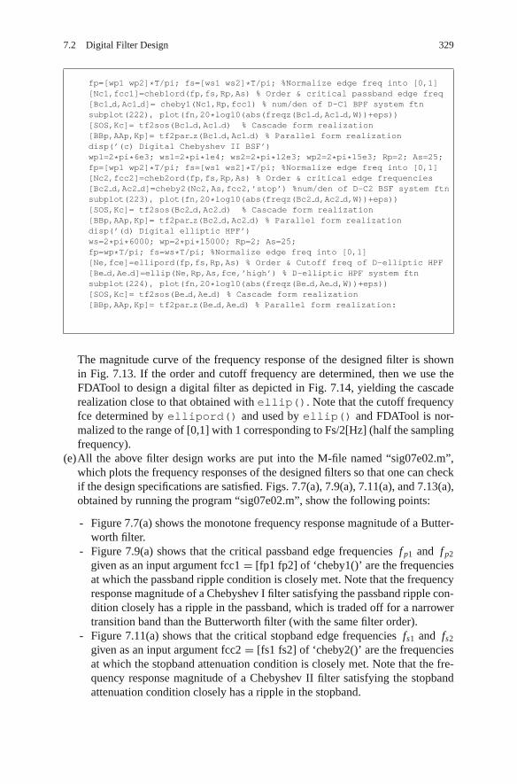
7.2 Digital Filter Design 329
fp=[wp1 wp2]*T/pi; fs=[ws1 ws2]*T/pi; %Normalize edge freq into [0,1][Nc1,fcc1]=cheb1ord(fp,fs,Rp,As) % Order & critical passband edge freq[Bc1 d,Ac1 d]= cheby1(Nc1,Rp,fcc1) % num/den of D-C1 BPF system ftnsubplot(222), plot(fn,20*log10(abs(freqz(Bc1 d,Ac1 d,W))+eps))[SOS,Kc]= tf2sos(Bc1 d,Ac1 d) % Cascade form realization[BBp,AAp,Kp]= tf2par z(Bc1 d,Ac1 d) % Parallel form realizationdisp(’(c) Digital Chebyshev II BSF’)wp1=2*pi*6e3; ws1=2*pi*1e4; ws2=2*pi*12e3; wp2=2*pi*15e3; Rp=2; As=25;fp=[wp1 wp2]*T/pi; fs=[ws1 ws2]*T/pi; %Normalize edge freq into [0,1][Nc2,fcc2]=cheb2ord(fp,fs,Rp,As) % Order & critical edge frequencies[Bc2 d,Ac2 d]=cheby2(Nc2,As,fcc2,’stop’) %num/den of D-C2 BSF system ftnsubplot(223), plot(fn,20*log10(abs(freqz(Bc2 d,Ac2 d,W))+eps))[SOS,Kc]= tf2sos(Bc2 d,Ac2 d) % Cascade form realization[BBp,AAp,Kp]= tf2par z(Bc2 d,Ac2 d) % Parallel form realizationdisp(’(d) Digital elliptic HPF’)ws=2*pi*6000; wp=2*pi*15000; Rp=2; As=25;fp=wp*T/pi; fs=ws*T/pi; %Normalize edge freq into [0,1][Ne,fce]=ellipord(fp,fs,Rp,As) % Order & Cutoff freq of D-elliptic HPF[Be d,Ae d]=ellip(Ne,Rp,As,fce,’high’) % D-elliptic HPF system ftnsubplot(224), plot(fn,20*log10(abs(freqz(Be d,Ae d,W))+eps))[SOS,Kc]= tf2sos(Be d,Ae d) % Cascade form realization[BBp,AAp,Kp]= tf2par z(Be d,Ae d) % Parallel form realization:
The magnitude curve of the frequency response of the designed filter is shownin Fig. 7.13. If the order and cutoff frequency are determined, then we use theFDATool to design a digital filter as depicted in Fig. 7.14, yielding the cascaderealization close to that obtained with ellip(). Note that the cutoff frequencyfce determined by ellipord() and used by ellip() and FDATool is nor-malized to the range of [0,1] with 1 corresponding to Fs/2[Hz] (half the samplingfrequency).
(e)All the above filter design works are put into the M-file named “sig07e02.m”,which plots the frequency responses of the designed filters so that one can checkif the design specifications are satisfied. Figs. 7.7(a), 7.9(a), 7.11(a), and 7.13(a),obtained by running the program “sig07e02.m”, show the following points:
- Figure 7.7(a) shows the monotone frequency response magnitude of a Butter-worth filter.
- Figure 7.9(a) shows that the critical passband edge frequencies f p1 and f p2
given as an input argument fcc1 = [fp1 fp2] of ‘cheby1()’ are the frequenciesat which the passband ripple condition is closely met. Note that the frequencyresponse magnitude of a Chebyshev I filter satisfying the passband ripple con-dition closely has a ripple in the passband, which is traded off for a narrowertransition band than the Butterworth filter (with the same filter order).
- Figure 7.11(a) shows that the critical stopband edge frequencies fs1 and fs2
given as an input argument fcc2 = [fs1 fs2] of ‘cheby2()’ are the frequenciesat which the stopband attenuation condition is closely met. Note that the fre-quency response magnitude of a Chebyshev II filter satisfying the stopbandattenuation condition closely has a ripple in the stopband.

330 7 Analog and Digital Filters
0[dB]
–20
–40
–60
–800 0.2 0.4 1.0
0
–10
–20
–30
–40
0 0.2 1.0
[dB]
Normalized frequency Normalized frequency (xπ rad/sample)
(a) From MATLAB (b) From the FDAtool
–As
–Rp
fs fp
Fig. 7.13 The magnitude curves of the frequency response of the digital elliptic HPF
Fig. 7.14 Design of a digital elliptic HPF with order 2 and stopband/passband edge frequencies0.24/0.6 using FDAtool (version 7.2-R2006a)

7.2 Digital Filter Design 331
Fig. 7.15 The state diagram of a filter drawn by the ‘Realize Model’ function of FDAtool
- Figure 7.13(a) shows that the critical passband edge frequency f p given as aninput argument fce of ‘ellip()’ is the frequency at which the passband ripplecondition is closely met. Note that the frequency response magnitude of anelliptic filter has ripples in both the passband and the stopband, yielding arelatively narrow transition band with the smallest filter order N = 2 amongthe four filters.
Note that we can click the Realize Model button or the Pole/Zero Editor buttonon the left-hand side of the FDATool window to create a Simulink model filehaving the designed filter block as depicted in Fig. 7.15 or to see the pole/zeroplot of the designed filter as illustrated in Fig. 7.14.
7.2.2 FIR Filter Design
FIR filters are compared with IIR filters as follows:Advantages: Disadvantages:- FIR filters can have exactly linearphase.
- FIR filters require a much higherfilter order than IIR filters to achieve agiven level of performance.
- FIR filters are stable. - The delay of FIR filters is often muchgreater than that of an equalperformance IIR filter.
According to the signal processing toolbox user’s guide (page 2–16), FIR filterdesign methods cast into MATLAB functions are listed in Table 7.1.

332 7 Analog and Digital Filters
Table 7.1 FIR filter design methods
Windowing Apply windowing to truncated IDFT ofdesired “brick wall” filter
fir1(), fir2()
Multibands withtransition bands
Equiripple or least squares approach oversubbands of the frequency range
firpm(), firls()
Constrained leastsquares
Minimize squared integral error overentire frequency range subject tomaximum error constraints
fircls(), fircls1()
Arbitraryresponses
Arbitrary responses, including nonlinearphase and complex filters
cfirpm()
Raised cosine Lowpass response with smooth,sinusoidal transition
firrcos()
As discussed in Sect. 4.6, the phases of FIR filters having symmetric or anti-symmetric coefficients are linear so that the phase delay τp and group delay τg areequal and constant over the frequency band, where the phase delay and group delayare related to the phase shift θ (Ω) = ∠G(Ω) of the frequency response as
τp = −θ (Ω)
Ωand τg = −dθ (Ω)
dΩwith θ (Ω) = ∠G(Ω)(phase response) (7.2.5)
Table 7.2 shows some restrictions on the frequency response depending on the sym-metry of the FIR filter (tap) coefficients g[n] and whether the filter order is even orodd. Note that fir1(N,fc,‘high’) and fir1(N,[fc1 fc2], ‘stop’) with an odd filter orderN design an (N + 1)th-order HPF and BSF (of type I), respectively since no linearphase HPF or BSF of odd order (type II) can be made.
Table 7.2 FIR filter design methods (see Sect. 4.6)
Linear phasefilter type
Filter order N Symmetry of filter (tap)coefficients g[n]
Restriction on frequencyresponse
Type I Even Symmetricg[n] = g[N − n]for n = 0 : N
No restriction
Type II Odd Symmetricg[n] = g[N − n]for n = 0 : N
G(Ω)|Ω=π = 0(No HPF or BSF)
Type III Even Anti-symmetricg[n] = −g[N − n]for n = 0 : N
G(Ω)|Ω=0 = 0,
G(Ω)|Ω=π = 0(No LPF or HPF or BSF)
Type IV Odd Anti-symmetricg[n] = −g[N − n]for n = 0 : N
G(Ω)|Ω=0 = 0 (No LPF)

7.2 Digital Filter Design 333
7.2.2.1 Windowing Method
Consider the frequency response of an ideal (“brick wall”) LPF with cutoff fre-quency Ωc as
G I (Ω) = G I [e jΩ] ={
1 for |Ω − 2mπ | ≤ Ωc ≤ π (m : an integer)
0 elsewhere(7.2.6)
Referring to Eq. (E3.5.2), we can take the inverse DTFT of this frequency responseto write the impulse response of an ideal LPF as
gI [n] = F−1{G I (Ω)} (3.1.3)= 1
2π
∫ Ωc
−Ωc
G(Ω)e jΩndΩ = Ωc
πsinc
(Ωcn
π
)(7.2.7)
Since this infinite-duration impulse response cannot be realized by a FIR filter, weapply a (rectangular) window of, say, length N + 1 (N = 2M : an even number) totruncate it to make the tap coefficients of an N th-order FIR LPF as
gL P [n] = gI [n]r2M+1[n + M] = Ωc
πsinc
(Ωcn
π
)for − M ≤ n ≤ M(M = N
2)
(7.2.8)We can multiply this with 2 cos(Ωpn) (for modulation) to obtain the tap coeffi-
cients of an N th-order FIR BPF with passband center frequency Ωp and bandwidth2Ωc as
gB P [n] = 2gL P [n] cos(Ωpn) for − M ≤ n ≤ M(M = N
2) (7.2.9)
We can also get the tap coefficients of N th-order FIR HPF (with cutoff fre-quency Ωc) and BSF (with stopband center frequency Ωs and bandwidth 2Ωc) bysubtracting the tap coefficients of LPF and BPF from the unit impulse sequenceδ[n] as
gH P [n] = δ[n] − gL P [n] = δ[n] − Ωc
πsinc
(Ωcn
π
)for − M ≤ n ≤ M(M = N/2)
(7.2.10)
gBS[n] = δ[n] − gB P [n] = δ[n] − 2gL P [n] cos(Ωsn) for − M ≤ n ≤ M(M = N/2)(7.2.11)
where δ[n] is the impulse response of an all-pass filter with a flat frequency response(see Example 3.4). Note the following:
- The tap coefficients or impulse responses of FIR filters (7.2.8), (7.2.9), (7.2.10),and (7.2.11) should be delayed by M = N/2 to make the filters causal forphysical realizability (see Sect. 1.2.9).

334 7 Analog and Digital Filters
- Cutting off the impulse response of an ideal filter abruptly for truncation resultsin ripples near the band edge of the frequency response. Thus a non-rectangularwindow such as a Hamming window is often used to reduce the Gibbs effect.
Given a filter order N and description of the desired frequency response including6dB band edge frequency (vector), the MATLAB functions fir1() and fir2()return the N + 1 tap coefficients of a FIR filter designed by the windowing method.Let us try using the MATLAB functions for FIR filter design in the followingexamples:
Example 7.3 Standard Band FIR Filter DesignLet us design several standard band FIR filters with sampling frequency Fs = 50
[kHz]. The following program “sig07e03.m” finds the tap coefficients of an LPFwith cutoff frequency 5kHz, a BPF with passband 7.5 ∼ 17.5kHz, a HPF withcutoff frequency 20kHz, and a BSF with stopband 7.5 ∼ 17.5kHz by usingEqs. (7.2.8), (7.2.9), (7.2.10), and (7.2.11) and the MATLAB function fir1().Fig. 7.16 shows the impulse responses (tap coefficients) and frequency responses ofthe filters obtained by running the program.
%sig07e03.m to design standard band FIR filtersclear, clfFs= 5e4; T=1/Fs; % Sampling frequency and sampling periodN=30; M=N/2; % Filter order and its halfnn=[-M:M]; nn1=nn+M; % Duration of filter impulse responsefn=[0:512]/512; W= fn*pi; % normalized and digital frequency ranges% LPF designfc LP= 5000*T*2; % Normalized 6dB cutoff frequency corresponding to 5kHzgLP= fc LP*sinc(fc LP*nn); % Eq. (7.2.8)gLP1= fir1(N,fc LP); % filter impulse response or tap coefficientsGLP= abs(freqz(gLP,1,W))+eps; GLP1= abs(freqz(gLP1,1,W))+eps;subplot(421), stem(nn1,gLP), hold on, stem(nn1,gLP1,’r.’)subplot(422), plot(fn,20*log10(GLP), fn,20*log10(GLP1),’r:’)% BPF designfc BP=[7500 17500]*T*2; % Normalized 6dB band edge frequenciesfp= sum(fc BP)/2*pi; % Passband center frequency[rad/sample]gBP= 2*gLP.*cos(fp*nn); % Eq. (7.2.9)gBP1= fir1(N,fc BP); % filter impulse response or tap coefficientsGBP= abs(freqz(gBP,1,W))+eps; GBP1= abs(freqz(gBP1,1,W))+eps;subplot(423), stem(nn1,gBP), hold on, stem(nn1,gBP1,’r.’)subplot(424), plot(fn,20*log10(GBP), fn,20*log10(GBP1),’r:’)% HPF designimpulse delayed= zeros(1,N+1); impulse delayed(M+1)= 1; % Impulsefc HP= 20000*T*2; % Normalized 6dB cutoff frequency 20kHzgHP= impulse delayed-fc HP*sinc(fc HP*nn); % Eq. (7.2.10)gHP1=fir1(N,fc HP,’high’); %filter impulse response/tap coefficientsGHP= abs(freqz(gHP,1,W))+eps; GHP1= abs(freqz(gHP1,1,W))+eps;subplot(425), stem(nn1,gHP), hold on, stem(nn1,gHP1,’r.’)subplot(426), plot(fn,20*log10(GHP), fn,20*log10(GHP1),’r:’)% BSF designfc BS=[7500 17500]*T*2; % Normalized 6dB band edge frequencies

7.2 Digital Filter Design 335
0.3
0.2
0.1
0
–0.10 5(a1) Impulse response (tap coefficients) of FIR LPF
10 15 20 25 30n
: Rectangular windowed: Hamming windowed
0.4
0.2
0
–0.2
–0.4
(a2) Impulse response (tap coefficients) of FIR BPF0 5 10 15 20 25 30n
0.2
0.1
0
–0.1
–0.2
(a3) Impulse response (tap coefficients) of FIR HPF0 5 10 15 20 25 30n
0.6
0.4
0.2
0
–0.20 5 10 15 20 25 n 30
(a4) Impulse response (tap coefficients) of FIR BSF
0[dB]–20
–40
–60
–800 0.2 0.3 0.5 0.7 0.8 1Ω/π
–6dB
(b1) Magnitude of frequency response of FIR LPF
: Rectangular windowed: Hamming windowed
0[dB] –6dB –6dB–20
–40
–60
–800 0.2 0.3 0.5 0.7 0.8 1Ω/π(b2) Magnitude of frequency response of FIR BPF
–6dB0
[dB]–20
–40
–60
–800 0.2 0.3 0.5 0.7 0.8 1Ω/π
(b3) Magnitude of frequency response of FIR HPF
–6dB–6dB0
[dB]–20
–40
–60
–800 0.2 0.3 0.5 0.7 0.8 1Ω/π
(b4) Magnitude of frequency response of FIR BSF
Fig. 7.16 Impulse responses (tap coefficients) and frequency responses of FIR filters
Ws= sum(fc BS)/2*pi; % Stopband center frequency[rad/sample]fc LP= (fc BS(2)-fc BS(1))/2; gLP= fc LP*sinc(fc LP*nn);gBS= impulse delayed-2*gLP.*cos(Ws*nn); % Eq. (7.2.11)gBS1=fir1(N,fc BS,’stop’); % filter impulse response/tap coefficientsGBS= abs(freqz(gBS,1,W))+eps; GBS1= abs(freqz(gBS1,1,W))+eps;subplot(427), stem(nn1,gBS), hold on, stem(nn1,gBS1,’r.’)subplot(428), plot(fn,20*log10(GBS), fn,20*log10(GBS1),’r:’)
7.2.2.2 Multi-Band FIR Filter Design
We can use the MATLAB function fir1(N,f,‘DC-1’) or fir1(N,f,‘DC-0’) to design FIR filters whose frequency response magnitude is close to [1 0 10 . . .] or [0 1 0 1 . . .] for each band [f(1) ∼ f(2) f(2) ∼ f(3) f(3) ∼ f(4) f(4) ∼f(5) . . .] between the neighboring edge frequencies. We can also use the MATLABfunction fir2(N,f,A) or firpm(N,f,A) or firls(N,f,A) to design FIR

336 7 Analog and Digital Filters
filters whose frequency response magnitude is close to an arbitrary piecewise linearshape specified by the second and third input arguments f and A. Note the following:
- The firpm() function implements the Parks-McClellan algorithm, which uses theRemez exchange algorithm and Chebyshev approximation theory to design mini-max or equiripple filters minimizing the maximum error between the desired andactual frequency responses [W-3]. It yields the frequency response exhibiting anequiripple behavior.
- The firls() function minimizes the integral of the squared error between thedesired and actual frequency responses.
- The number of desired frequency-amplitude points must be even for firpm()and firls().
- While the desired frequency response for fir1() is supposed to be the brick walltype, firpm and firls() allow us to describe the desired frequency response so thatwe can insert the transition band(s) between the passband(s) and stopband(s) toreduce the ripple in the magnitude of the frequency response.
Example 7.4 Multi-Band FIR Filter DesignFigure 7.17 shows the impulse responses (tap coefficients) and frequency
responses of the filters obtained by running the following program “sig07e04.m”.Especially, Fig. 7.17(b4) illustrates the difference between the magnitude responsesof the equiripple and LSE filters that are designed using firpm() and firls(),respectively.
%sig07e04.m% to design multi-band FIR filters using fir1()/fir2()/firpm()clear, clffn=[0:512]/512; W= fn*pi; % normalized and digital frequency rangesN=30; M=N/2; % Filter order and its halfnn=[-M:M]; nn1=nn+M; % Duration of filter impulse response%Multi pass/stop-band filter using fir1()ffe=[0.2 0.4 0.6 0.8]; % Band edge frequency vectorB fir1 DC1=fir1(N,ffe,’DC-1’); % Tap coefficient vectorG fir1 DC1= freqz(B fir1 DC1,1,W); % Frequency response magnitudesubplot(421), stem(nn1,B fir1 DC1)subplot(422), plot(fn,abs(G fir1 DC1))%Multi stop/pass-band filter using fir1()B fir1 DC0=fir1(N,ffe,’DC-0’); % Tap coefficient vectorG fir1 DC0= freqz(B fir1 DC0,1,W); % Frequency response magnitudesubplot(423), stem(nn1,B fir1 DC0)subplot(424), plot(fn,abs(G fir1 DC0))%Multi pass/stop-band filter using fir2()% Desired piecewise linear frequency responseffd=[0 0.18 0.22 0.38 0.42 0.58 0.62 0.78 0.82 1]; % Band edges in pairsGGd=[1 1 0 0 1 1 0 0 1 1];B fir2=fir2(N,ffd,GGd);G fir2= freqz(B fir2,1,W);subplot(425), stem(nn1,B fir2)subplot(426), plot(fn,abs(G fir2), ffd,GGd,’k:’)

7.2 Digital Filter Design 337
%Multi-band pass/stop filter using firpm()B firpm=firpm(N,ffd,GGd); % The number of frequency points must be evenB firls=firls(N,ffd,GGd); % The number of frequency points must be evenG firpm= freqz(B firpm,1,W);G firls= freqz(B firls,1,W);subplot(427), stem(nn1,B firpm), hold on, stem(nn1,B firls,’.’)subplot(428), plot(fn,abs(G firpm), fn,abs(G firls),’r-.’, ffd,GGd,’k:’)
0.5
0
0 5 10 15 20 25 30
0 5 10 15 20 25 30
0 5 10 15 20 25 30
0 5 10 15 20 25 30
0.40.2
–0.20
0.40.6
0.2
–0.20
0.40.6
0.2
–0.20
0.5
1
0
0.5
1
0
0.5
1
0
0.5
1
00 0.1 0.2 0.3 0.4 0.6 0.70.5 0.8 1Ω/π
0.50 0.1 0.2 0.3 0.4 0.6 0.70.5 0.8 1Ω/π
0.50 0.1 0.2 0.3 0.4 0.6 0.7 0.8 1Ω/π
0.50 0.1 0.2 0.3 0.4 0.6 0.70.5 0.8 1Ω/π(a1) Impulse response of multi-band FIR filter designed by using fir1(30,ffe, ‘DC–1’)
(a2) Impulse response of multi-band FIR filter designed by using fir1(30,ffe, ‘DC–0’)
(a3) Impulse response of multi-band FIR filter designed by using fir2(30,fd,Gd)
(a4) Impulse response of multi-band FIR filter designed by using firpm(30,fd,Gd)/firls()
(b4) Magnitude response of multi-band FIR filter designed by using firpm(30,fd,Gd)/firls()
(b3) Magnitude response of multi-band FIR filter designed by using fir2(30,fd,Gd)
(b2) Magnitude response of multi-band FIR filter designed by using fir1(30,ffe,’DC–0’)
(b1) Magnitude response of multi-band FIR filter designed by using fir1(30,ffe, ‘DC–1’)
n
n
n
n
firpm()firls()
Desired magnitude responseActual magnitude response
firpm()firls()
Fig. 7.17 Multi-band FIR filters designed using fir1(), fir2(), and firpm()/firls()
7.2.2.3 Anti-Symmetric FIR Filter Design
We can use the MATLAB functions firpm() or firls() with the fourth inputargument ‘h’ or ‘d’ to design anti-symmetric FIR filters. Note that in the ‘d’mode, firpm() and firls() weight the error by 1/Ω and 1/Ω2, respectivelyin nonzero amplitude bands to minimize the maximum relative error or sum of rel-ative squared error. Note from Table 7.2 that the desired frequency response of an

338 7 Analog and Digital Filters
anti-symmetric FIR filter of an even order should be allowed to be zero at Ω = 0and π and that of an anti-symmetric FIR filter of an odd order should be allowed tobe zero at Ω = 0.
Example 7.5 Anti-Symmetric Filters – Hilbert Transformer and Differentiator
(a)Hilbert TransformerThe impulse response of the Hilbert transformer dealt with in Problems 2.10and 3.2 has an odd symmetry so that it can easily be designed using firpm()or firls() with the fourth input argument ‘h’ as in the following program“sig07e05a.m”. We can run it to get Fig. 7.18, where the frequency response ofthe ideal Hilbert transformer is
H (Ω)(P3.2.1)=
{− j for 0 < Ω < π
+ j for − π < Ω < 0(7.2.12)
%sig07e05a.m% to design Hilbert transformers as anti-symmetric FIR filters% by using firpm() or firls().clear, clffn=[0:512]/512; W= fn*pi; % normalized and digital frequency ranges% Hilbert transformer using firpm() or firls()% Type III (anti-symmetric and even order) with G(0)=0 and G(pi)=0B20 H firpm= firpm(20,[0.05 0.95],[1 1],’h’); % Type IIIG20 H firpm= freqz(B20 H firpm,1,W);B20 H firls= firls(20,[0.05 0.95],[1 1],’h’); % Type IIIG20 H firls= freqz(B20 H firls,1,W);% Type IV (anti-symmetric and odd order) with G(0)=0B21 H firpm= firpm(21,[0.05 1],[1 1],’h’); % Type IVG21 H firpm= freqz(B21 H firpm,1,W);B21 H firls= firls(21,[0.05 1],[1 1],’h’); % Type IVG21 H firls= freqz(B21 H firls,1,W);subplot(421), nn=[0:20]; % Duration of filter impulse responsestem(nn,B20 H firpm), hold on, stem(nn,B20 H firls,’.’)subplot(422), plot(fn,abs(G20 H firpm), fn,abs(G20 H firls),’:’)subplot(423), nn=[0:21]; % Duration of filter impulse responsestem(nn,B21 H firpm), hold on, stem(nn,B21 H firls,’.’)subplot(424), plot(fn,abs(G21 H firpm), fn,abs(G21 H firls),’:’)% Use filter visualization tool to see the filterfvtool(B20 H firpm,1,B20 H firls,1)fvtool(B21 H firpm,1,B21 H firls,1)
(b)DifferentiatorThe impulse response of the differentiator dealt with in Problem 3.3 has an oddsymmetry so that it can easily be designed by using firpm() or firls()with the fourth input argument ‘d’ as in the following program “sig07e05b.m”where firpm() and firls() in the ‘d’ mode weight the error by 1/Ω and1/Ω2, respectively. We can run it to get Fig. 7.19.

7.2 Digital Filter Design 339
(Q)Why is the rightmost edge frequency in the second input argument of firpm()/firls()set to 0.95 instead of 1 for the type III FIR filter design despite the nonzerodesired magnitude response at Ω = π ?
0.5
0
0(a1) Impulse response of a Hilbert transformer
using firpm()/firls (20, [0.05,0.95], [1 1], 'h')
(a2) Impulse response of a Hilbert transformer using firpm()/firls (21, [0.05,1], [1 1], 'h')
(b2) Magnitude response of a Hilbert transformerusing firpm()/firls (21, [0.05,1], [1 1], 'h')
(b1) Magnitude response of a Hilbert transformer using firpm()/firls (20, [0.05,0.95], [1 1], 'h')
5 10
: firpm(): firls()
: firpm(): firls()
: firpm(): firls()
: firpm(): firls()
15 20n 0 0.2 0.4 0.6 0.8 1Ω/π
–0.5
0.5
0
0 5 10 15 2021n
–0.5
0.5
1
0
0 0.2 0.4 0.6 0.8 1Ω/π
0.5
1
0
Fig. 7.18 Hilbert transformers designed using firpm() and firls()
0 5 10 15 20 21n
0 5 10 15 20n
1
–1
0
1
–1
01
0
3
2
1
0
3
2
0 0.2 0.4 0.6 0.8 1Ω/π
0 0.2 0.4 0.6 0.8 1Ω/π
firpm()firls()
firpm()firls()
firpm()firls()
firpm()firls()
(a1) Impulse response of a differentiator using firpm()/firls(20,[0 0.95],[0 0.95*pi], ‘d’)
(a2) Impulse response of a differentiator using firpm()/firls(21,[0 1],[0 pi], ‘d’)
(b1) Magnitude response of a differentiator using firpm()/firls(20,[0 0.95],[0 0.95*pi], ‘d’)
(b2) Magnitude response of a differentiator using firpm()/firls(21,[0 1],[0 pi], ‘d’)
Fig. 7.19 Differentiators designed using firpm() and firls()

340 7 Analog and Digital Filters
%sig07e05b.m% to design differentiators as anti-symmetric FIR filters% by using firpm() or firls().clear, clffn=[0:512]/512; W= fn*pi; % normalized and digital frequency ranges% Differentiator using firpm()or firls()B20 d firpm= firpm(20,[0 0.95],[0 0.95*pi],’d’); % Type IIIG20 d firpm= freqz(B20 d firpm,1,W);B20 d firls= firls(20,[0 0.95],[0 0.95*pi],’d’); % Type IIIG20 d firls= freqz(B20 d firls,1,W);B21 d firpm= firpm(21,[0 1],[0 pi],’d’); % Type IV with G(0)=0G21 d firpm= freqz(B21 d firpm,1,W);B21 d firls= firls(21,[0 1],[0 pi],’d’); % Type IV with G(0)=0G21 d firls= freqz(B21 d firls,1,W);subplot(421), nn=[0:20]; % Duration of filter impulse responsestem(nn,B20 d firpm), hold on, stem(nn,B20 d firls,’.’)subplot(422), plot(fn,abs(G20 d firpm), fn,abs(G20 d firls),’:’)subplot(423), nn=[0:21]; % Duration of filter impulse responsestem(nn,B21 d firpm), hold on, stem(nn,B21 d firls,’.’)subplot(424), plot(fn,abs(G21 d firpm), fn,abs(G21 d firls),’:’)% Use filter visualization tool to see the filterfvtool(B20 d firpm,1,B20 d firls,1)fvtool(B21 d firpm,1,B21 d firls,1)
7.2.2.4 Constrained Least Squares (CLS) FIR Filter Design
There are two CLS filter design functions, fircls() and fircls1(). Thefircls() function designs FIR filters whose magnitude responses are close tothe desired piecewise constant one specified by a vector of band edges and thecorresponding vector of band amplitudes. The upperbound and lowerbound of thedesired magnitude response can also be given. The fircls1() function designsa FIR LPF or HPF whose magnitude response is close to the brick wall type forthe passband/stopband specified by the cutoff frequency within the given toleranceon the passband and stopband ripples. Given the passband and stopband edge fre-quencies together with the weighting factor on stopband error relative to passbanderror, it applies the weighted least squares algorithm. In the case of HPF design, thefilter order N given as the first input argument should be even; otherwise, it will beincremented by one to make an even filter order.
Example 7.6 Multi-Band CLS FIR Filter DesignThe MATLAB function fircls() is used to design a two-band FIR filter with
the desired magnitude response vector A = [0 0.5 0 1 0] for the bands speci-fied by the band edge vector f = [0 0.3 0.5 0.7 0.9 1] in the following program“sig07e06.m”. We run it to get Fig. 7.20, which shows the magnitude responsesof the two filters where filter 1 and filter 2 are designed with the upperbound andlowerbound stricter on the stopband and the passband, respectively.

7.2 Digital Filter Design 341
Fig. 7.20 Multiband FIR filters designed using fircls(30,f,A,ub,lb) with f = [0 0.3 0.5 0.7 0.8 1]and A = [0 0.5 0 1 0]
(cf) We can change the unit of magnitude and frequency scale in the AnalysisParameters dialog box opened by clicking Analysis/Analysis Parameters onthe menu bar of the Filter Visualization window.
%sig07e06.m% CLS design multi-band filters using fircls().clear, refresh(1)N=50; % Filter orderf= [0 0.3 0.5 0.7 0.8 1]; % The band edge frequency vectorA= [0 0.5 0 1 0]; % The magnitude response vectorub1= [0.01 0.54 0.02 1.05 0.02]; lb1= [-0.01 0.46 -0.02 0.95 -0.02];B1 fircls= fircls(N,f,A,ub1,lb1); % stricter on stopband ripple conditionub2= [0.05 0.51 0.05 1.02 0.05]; lb2= [-0.05 0.49 -0.05 0.98 -0.05];B2 fircls= fircls(N,f,A,ub2,lb2); % stricter on passband ripple conditionfvtool(B1 fircls,1, B2 fircls,1) %filter visualization tool to see filter% Click any point on the frequency curve to add data markers
Example 7.7 CLS FIR LPF/HPF Design
(a)FIR LPF DsignWe can run the following program “sig07e07a.m” to get Fig. 7.21(a), whichshows the magnitude responses of the two filters where filter 2 is designed withmore weighting (Kw > 1) on the stopband.
%sig07e07a.m% to CLS design LPF filters using fircls1().clear, refresh(1)N=30; fc= 0.3; % Filter order and Cutoff frequencyfp=0.28; fs=0.32; % Passband and stopband edge frequenciesrp= 0.05; rs= 0.02; % Tolerances on passband and stopband ripple% FIR LPF design using fircls1()B1 LPF fircls1= fircls1(N,fc,rp,rs);Kw=10; % For more weighting on the stopband ripple conditionB2 LPF fircls1= fircls1(N,fc,rp,rs,fp,fs,Kw);% Use filter visualization tool to see the filterfvtool(B1 LPF fircls1,1, B2 LPF fircls1,1)

342 7 Analog and Digital Filters
(b)FIR HPF DsignWe can run the following program “sig07e07b.m” to get Fig. 7.21(b), whichshows the magnitude responses of the three filters where filters 2 and 3 aredesigned with more weighting (Kw < 1) on the passband. Note that filters 2/3are ensured to satisfy the passband/stopband ripple condition at the frequency offt = fp + 0.02/fs − 0.02, respectively.
%sig07e07b.m% to CLS design HPF filters using fircls1().clear, refresh(1)N=30; fc= 0.3; % Filter order and Cutoff frequencyfp=0.28; fs=0.32; % Passband and stopband edge frequenciesrp= 0.05; rs= 0.02; % tolerances on passband and stopband ripple% FIR HPF design using fircls1()B HPF fircls1= fircls1(N,fc,rp,rs,’high’);Kw=0.1; %more weighting on passband ripple condition% To ensure error(ft)<rp with ft within the passbandft=fp+0.02;B1 HPF fircls1= fircls1(N,fc,rp,rs,fp,fs,Kw,ft,’high’);% To ensure error(ft)<rs with ft within the stopbandft=fs-0.02;B2 HPF fircls1= fircls1(N,fc,rp,rs,fp,fs,Kw,ft,’high’);% Use filter visualization tool to see the filterfvtool(B HPF fircls1,1, B1 HPF fircls1,1, B2 HPF fircls1,1)
0
–10
–20
–30
–40
–50
0 0.1 0.2 0.3 Normalized Frequency (xπ rad/sample)
(a) The magnitude responses of FIR LPFs (b) The magnitude responses of FIR LPFs
1.0 0 0.1 0.2 0.3 Normalized Frequency (xπ rad/sample) 1.0
[dB]0
–10
–20
–30
–40
[dB]
Filter #2
Filter #1Filter #1Filter #2
Filter #3
Fig. 7.21 FIR LPF/HPFs designed using fircls1()
7.2.2.5 Arbitrary-Response FIR Filter Design
The cfirpm() function designs a possibly nonlinear phase, asymmetric, complex-coefficient, and equiripple frequency response FIR filter minimizing the Chebyshev(or minimax) error between the actual magnitude response and desired one. Notethe following:
- B = cfirpm(N, f, A, w) returns a length (N + 1) FIR filter whose magnituderesponse is the best approximation to the desired frequency response describedby f and A where
N: the filter order.

7.2 Digital Filter Design 343
f: the vector of (an even number of) band edge frequencies arranged in ascend-ing order between −1 and +1 where 1 is half the sampling frequency,i.e., the Nyquist frequency. The frequency bands span f(k) to f(k + 1) fork odd; the intervals f(k + 1) to f(k + 2) for k odd are “transition bands” or“don’t care regions” during optimization.
A: a real vector (of the same size as f) which specifies the desired magnituderesponse as the line connecting the points (F(k),A(k)) and (F(k+1), A(k+1)) for odd k.
W: a vector of real, positive weights, one per band, for use during optimization.If not specified, it is set to unity.
- For filters with a gain other than zero at Fs/2, e.g., highpass and bandstop filters,N must be even. Otherwise, N will be incremented by one.
- B = cfirpm(N, f, {@fresp, p1, p2, · · · }, w) returns a length (N + 1) FIR filterwhose magnitude is the best approximation to the desired frequency response asreturned by function @fresp with optional arguments p1,p2, · · · . The function iscalled from within cfirpm() using the syntax [fg, wg] = fresp(N, f, fg, w, p1, p2,
· · · ) where
fg: a vector of interpolated grid frequencies over each specified frequency bandat which the response function will be evaluated.
Ag and wg: the desired complex frequency response and optimization weightvectors, respectively, evaluated at each frequency in grid fg.
- Predefined frequency response functions for @fresp include:
‘lowpass’, ‘bandpass’, ‘hilbfilt’, ‘allpass’, ‘highpass’, ‘bandstop’, ‘differen-tiator’, ‘invsinc’
- B = cfirpm(· · · , Sym) imposes a symmetry constraint on the impulse response,where Sym may be one of the following:
‘none’: Default if any negative band edge frequencies are passed, or if @frespdoes not supply a default value of Sym.
‘even’: Impulse response will be real and even. This is the default for highpass,lowpass, bandpass, bandstop, and multiband designs.
‘odd’: Impulse response will be real and odd. This is the default for Hilbert anddifferentiator designs. The desired magnitude response at Ω = 0 mustbe zero.
‘real’: Impose conjugate symmetry on the frequency response.(cf) If any Sym option other than ‘none’ is specified, the band edges should only
be specified over positive frequencies; the negative frequency region willbe filled in from symmetry.
Example 7.8 Complex-Coefficient, Arbitrary Magnitude Response FIR Filter DesignThe MATLAB function cfirpm() is used to design two FIR filters with differ-
ent filter order N = 30 and 40, with the desired piecewise linear magnitude responseconnecting the frequency-amplitude points {(−1, 5), (−0.5, 1), (−0.4, 2), (0.3, 2),(0.4, 2), (0.9, 1)} in the following program “sig07e08.m”. We run it to get Fig. 7.22,which shows the impulse and magnitude responses of the two filters.

344 7 Analog and Digital Filters
(a1) Complex impulse response of 30th–order Filter 1 (a2) Complex impulse response of 40th–order Filter 2
0
2
–1 –0,5 0 0.5 1 –1 –0,5 0
(b2) Asymmetric frequency response of Filter 2Normalized Frequency (xπ rad/sample)
(b1) Asymmetric frequency response of Filter 1
(c) User–defined Spectral Mask dialog boxto the desired magnitude response
Normalized Frequency (xπ rad/sample)
: Desired magnitude response: Actual magnitude response
0.5 1
4
6
8
10
12
14[bB]
2
4
6
8
10
12
14[bB]
0 5 10 15 20 30
Filter #1: Real
Samples 0 5 10 15 20 25 30 40Samples
Filter #1: Imaginary
Filter #1: Real
Filter #1: Imaginary
0.5
1
1.5
2
0
0.5
1
1.5
2
: Desired magnitude response: Actual magnitude response
To plot the desired magnitude response curveso that it will be overlapped with the actual oneof the designed filter dotted, type in the bandedge frequency vector and the corrrespondingdesired magnitude response vector into thedialog box opened by clicking the View/User-defined Spectral Mask menu on the top menu bar.
(cf)
Fig. 7.22 Complex impulse response and frequency response of (nonlinear phase) FIR filtersdesigned using cfirpm()
%sig07e08.m% use cfirpm() to design FIR filters% having an arbitrary complex frequency response (with nonlinear phase)clear, refreshfor N=[30 40]
% Frequency/magnitude vectors describing desired frequency responsef=[-1 -0.5 -0.4 0.3 0.4 0.9];A=[5 1 2 2 2 1]; %[14 0 6 6 6 0](dB)Kw=[1 10 5]; % A vector describing the weighting factor for each bandB cfirpm= cfirpm(N,f,A,Kw);% Use filter visualization tool to see the filterfvtool(B cfirpm,1)
end

7.2 Digital Filter Design 345
7.2.3 Filter Structure and System Model Available in MATLAB
Figure 7.23 shows various filter structures that can be constructed, realized, and castinto a Simulink block by using FDATool or the dfilt()/realizemdl() command (seeSect. E.15). Note that all of the (transposed) direct I and II forms in Fig. 7.23(a)–(d)commonly have the following system function
bm3
bm3
–am3
–am2
–am3
–am2
bm2
bm1
bm1
bm2
z –1
z –1 z –1
z –1
z –1
z –1 z –1
z –1 z –1
z –1
z –1
z –1
z –1
z –1z –1
z –1z –1
z –1
z –1
z –1
y [n ]u [n ]Y [z ]
y [n ]
Y [z ]
U [z ]
u [n ]U [z ]
bm3–am3
–am2 bm2
bm1 y [n ]u [n ]Y [z ]U [z ]
u [n ]U [z ]
bm3 –am3
–am2
bm1
bm2
z –1
z –1
z –1
y [n ]
Y [z ]u [n ]U [z ]
(a) Direct I form – SOS (cascade)
(c) Direct II form – SOS (cascade)
(b) Transposed direct I form – SOS (cascade)
(d) Transposed direct II form – SOS (cascade)
y [n ]
Y [z ]
p1p2p3pN+1
z –1 z –1
– rN rN – r2 r2 – r1 r1
u [n ]U [z ]
z –1
y1[n ]
Y1[z ]
z –1 z –1
– rN rN – r2 r2
r2r2
– r1 r1
r1 r1
y2[n ]
Y2[z ]
All–pass output All-pole output
z –1 z –1 z –1
y2[n ]
Y2[z ]
y1[n ]
Y1[z ]
u [n ]U [z ]
rN rN Minimum-phaseoutputMaximum-phaseoutput
(e) Lattice/ladder –ARMA form
(f) IIR lattice form
(g) FIR lattice form
Fig. 7.23 Various filter structures

346 7 Analog and Digital Filters
b–Mf
u [n]U [z]
u [n]U [z ]
u [n ]U [z ]
y [n ]Y [z ]
y [n]Y [z]
b–1
–a1
–aN–1
–aN
–a1
–aN –1
–aN
z–1
z–1
z–1
z–1
z–1 z–1
z–1
z–1
z–1
z–1
z
z b0
b1
bMb
b–Mf
b–1
z–1
z–1
z–1
z
zb0
b1
bMb
b0 b1 b2
u [n ]U [z ]
z–1
z–1 z–1
z–1
z–1
z–1
z–1
b0 b1 b2 b3
u [n ]U [z ]
z–1
z–1 z–1
z–1
z–1
z–1
z–1
b0 b1 b2 b3
u [n ]U [z ]
z–1
z–1 z–1
z–1
z–1
b0
–1 –1 –1 –1 –1 –1
b1 b2
(h) Direct I form (i) Direct II form
(j2) Direct symmetric form with an odd order
(k2) Direct asymmetric form with an odd order
( j1) Direct symmetric form with an even order
(k1) Direct asymmetric form with an even order
Fig. 7.23 (continued)
G[z] = K G M+1[z]MΠ
m=1Gm[z] = K
bM+1,1z + bM+1,2
z + aM+1,2
MΠ
m=1
bm1z2 + bm2z + bm3
z2 + am2z + am3
with M = floor(N
2) (7.2.13)
MATLAB represents the SOSs (second-order sections) connected in cascade(with the output of each stage applied into the input of the next stage) as an M × 6array ‘SOS’, each row of which contains the numerator and denominator coefficientvector [bm1 bm2 bm3 1 am2 am3] of a single section.
MATLAB provides several functions that can be used for conversion betweenthe various linear system models as listed in Table 7.3. Converting from one systemmodel or filter structure to another may yield a result with different characteristicthan the original due to the computer’s finite-precision arithmetic operations and thevariations in the conversion’s round-off computations.

7.2 Digital Filter Design 347
Tabl
e7.
3M
AT
LA
Bfu
nctio
nsfo
rco
nver
sion
betw
een
the
vari
ous
linea
rsy
stem
mod
els
Syst
emFu
nctio
nSt
ate-
Spac
eZ
ero-
Pole
-Gai
nSO
S(c
asca
de)
SOS
(par
alle
l)L
attic
e
Syst
emFu
nctio
n—
tf2ss()
tf2zp()
tf2sos()
tf2parz()
∗tf2latc()
Stat
e-Sp
ace
ss2tf()
—ss2zp()
ss2sos()
Non
eN
one
Zer
o-Po
le-G
ain
zp2tf()
zp2ss()
—zp2sos()
Non
eN
one
SOS
(cas
cade
)sos2tf()
sos2ss()
sos2zp()
—N
one
Non
eSO
S(p
aral
lel)
par2tf()
∗N
one
Non
eN
one
—N
one
Lat
tice
latc2tf()
Non
eN
one
Non
eN
one
—
(cf)
∗m
eans
that
the
MA
TL
AB
func
tion
isfa
bric
ated
inth
isbo
ok.

348 7 Analog and Digital Filters
In the Filter Design & Analysis window (Fig. 7.24(a)) opened by typing ‘fdatool’in the MATLAB command window, we can convert the structure of a designedfilter through the Convert Structure dialog box (Fig. 7.24(b1)) opened by clickingEdit/Convert Structure (Fig. 7.24(b)) on the top menu bar. The following structuresare available for conversion in MATLAB:
- Direct form I, Direct form II, Direct form I transposed, or Direct form IItransposed
- Second-Order Sections- Lattice minimum/maximum phase from minimum/maximum-phase FIR filter- Lattice allpass from Allpass filter- Lattice ARMA from IIR filter- State-Space model
The MATLAB function dfilt() can also be used to convert the filter structure. Forexample,
>>B=firls(30,[0 .5 .6 1],[0 0 1 1]); Gd1=dfilt.dffir(B); %direct-form FIR>>[B,A]=butter(7,0.2); Gd2=dfilt.df2tsos(tf2sos(B,A)); %direct IIt-SOS IIR>>Gd par=dfilt.parallel(Gd1,Gd2); %parallel structure of two or more objects>>realizemdl(Gd par) % To create Simulink model>>fvtool(Gd1,Gd2,Gd par) % To analyze filter
7.2.4 Importing/Exporting a Filter Design
In the FDATool window (Fig. 7.24), we can click the Import Filter button in the sidebar to open the Import Filter panel (Fig. 7.25) and import a filter in any of the repre-sentations in the Filter Structure or a SOS by clicking on the check box. In the fieldsof Numerator and Denominator, type the filter coefficient vectors explicitly or thenames of the variables whose values are in the MATLAB workspace. Then selectthe frequency unit from the options in the Units menu and if the selected frequencyunit is not ‘Normalized’, specify the value or MATLAB workspace variable of thesampling frequency in the Fs field. Lastly click the Import Filter button at the bottomof the Import Filter panel to import the filter that you have specified. You can editthe imported filter using the Pole/Zero Editor panel in which you can move poles,add, or delete poles/zeros.
On the other hand, we can select the File/Export menu in the FDATool windowto open the Export dialog box (Fig. 7.26) and save your filter design result by
- exporting the filter coefficients or objects to the workspace, a MAT-file, or a Cheader file,
- exporting the filter coefficients to an ASCII file,- or exporting to SPTool or Simulink.
(cf) FDATool GUI is opened through the Digital Filter Design block in the SignalProcessing Blockset.

7.2 Digital Filter Design 349
Fig. 7.24 FDA Tool window and its menu

350 7 Analog and Digital Filters
Fig. 7.25 Import Filter panel opened by clicking the Import Filter button in the side bar
Fig. 7.26 Exporting a filter design result
7.3 How to Use SPTool
SPTool is an interactive GUI for digital signal processing that can be used to
- Analyze signals (Signal Browser)- Design filters (FDATool: Filter Design & Analysis Tool)- Analyze (view) filters (FVTool: Filter Visualization Tool)- Filter signals- Analyze signal spectra (Spectrum Viewer)
Signals, filters, and spectra can be brought from the MATLAB workspace into theSPTool workspace using File/Import. Signals, filters, and spectra created/modifiedin or imported into the SPTool workspace can be saved (as MATLAB structures)using File/Export.
Figure 7.27(a) shows the SPTool window opened by typing ‘sptool’ into theMATLAB command window where you can access the three GUIs, i.e., Signal

7.3 How to Use SPTool 351
Fig. 7.27 SPTool window, Signal Browser window, and Spectrum Viewer window

352 7 Analog and Digital Filters
Browser (Fig. 7.27(b)), Filter Visualization Tool (Fig. 7.20(a)), and Spectrum Viewer(Fig. 7.27(c)) by selecting a signal, filter, or spectrum and clicking the appropriateView button. Note that if you start FVTool by clicking the SPTool Filter View button,FVTool is linked to SPTool so that any changes made in SPTool are immediatelyreflected in FVTool where the FVTool title bar includes “SPTool” to indicate thelink. (Every time you click the Filter View button, a new, linked FVTool starts,which allows you to view multiple analyses simultaneously. Any parameter exceptthe sampling frequency can be changed in a linked FVTool. The sampling frequencycan be changed through the Sampling Frequency dialog box opened by selecting theEdit/Sampling Frequency menu in the SPTool window or by selecting the Analy-sis/Sampling Frequency menu in the FDATool window, which will be opened byclicking the Filters/Edit button.) If you start an FVTool by clicking the New buttonor by selecting File/New from within FVTool, that FVTool is a stand-alone versionthat is not linked to SPTool. You can also access a reduced version of FDATool(Fig. 7.24(a)) by clicking the New button to create a new filter or the Edit button toedit a selected filter. You can apply a selected filter to a selected signal by clickingthe Apply button. Clicking the Create button opens the Spectrum Viewer and showsthe PSD (power spectral density) of the selected signal. Clicking the Update buttonopens the Spectrum Viewer for the selected spectrum.
Let us try using the SPTool in the following steps:
1. Create a noisy two-tone signal in the MATLAB workspace and import it intoSPTool.
2. Design a BPF using FDATool.3. Apply the designed filter to the signal to create a bandlimited noisy signal.4. Analyze the input and output signals. For example, you can compare the original
and filtered signals in the time domain using the Signal Browser.5. Compare the original and filtered signals in the frequency domain using the
Spectrum Viewer.6. Save the filter design and signal analysis results by exporting to disk (MAT-file)
or workspace.
<Step 1: Creating a noisy signal in the MATLAB workspace and importing itinto SPTool>You can type the following statements into the MATLAB command window:
>>Fs=1e4; Ts=1/Fs; tt=[0:Ts:0.5]; randn(’state’,0);>>x=sin(2*pi*941*tt)+cos(2*pi*1209*tt)+0.1*randn(size(tt));>>sptool % Open a SPTool window to start a new SPTool session
Then in the SPTool window, select the File/Import menu to open the Import-to-SPTool dialog box in which you can import x and Fs into the SPTool inthe following way (see Fig. 7.28(a)):
- Select x from the Workspace Contents list, click the upper Right-Arrowbutton, and name the signal by typing, say, ‘sig1’ (default name) in theName field to import x as a signal data.

7.3 How to Use SPTool 353
Fig. 7.28 Importing signal, designing filter, applying designed filter, and editing samplingfrequency
354 7 Analog and Digital Filters
- Select Fs from the workspace contents list and click the lower Right-Arrow button to import Fs as the sampling frequency.
- Click the OK button to close the Import-to-SPTool dialog box. Then youwill see sig1[vector] in the SPTool’s Signals list (see Fig. 7.29(a)).
(cf) You can also import signals from MAT-files on your disk.(cf) You can import filters and spectra into SPTool in the same way as you
import signals.
<Step 2: Using FDATool to design a BPF>
You might import an existing filter or design/edit a new filter using FDATool.Here, click the New button to open FDATool, type the following specificationinto the appropriate fields, and then click the Design Filter button to design afilter named ‘filt1’ by default (Fig. 7.28(b)):Sampling frequency: Fs = 10kHz, Stopband attenuation: As = 50dB, andPassband ripple: Rp = 3dB
Passband edge frequencies: f p1 = 1.1 kHz, f p2 = 1.8 kHzStopband edge frequencies: fs1 = 1 kHz, fs2 = 2kHz
<Step 3: Applying the designed filter to the signal to create a bandlimitedsignal>
- Select the signal ‘sig1[vector]’ from the Signals list by clicking on it(Fig. 7.27(a)).
- Select the filter ‘filt1[design]’ from the Filters list by clicking on it.- Click the Apply button under the Filters list to open the Apply Filter dialog
box (Fig. 7.28(c)), in which you can select the filtering algorithm, namethe output signal, say, ‘sig2’, and click OK to close the dialog box. Thenyou will see sig2[vector] in the SPTool’s Signals list.
(cf) If you see a warning message that the sampling frequencies for the sig-nal and filter are different, select the Edit/Sampling Frequency menu tomake them equal and then apply the filter to the signal(Fig. 7.28(d)).
<Step 4: Comparing the original and filtered signals in the time domain inSignal Browser>
- Select the signals ‘sig1’ and ‘sig2’ from the Signals list by (Shift/Ctrl+)clicking on them.
- Click the View button under the Signals list to open the Signal Browserwindow and see the two signals in the time domain.
- If needed or desired, you can click the Select Trace button to select one ofthe displayed signals and then click the Line Properties button to changethe color and/or line style to display the selected signal.
7.3 How to Use SPTool 355
- You can also click the Play Selected Signal button to play the selected sig-nal. You can click the Vertical Markers button to use the vertical Markersto select a portion of the signal you want to play. If you want to print thesignals (or their spectra), click the Print button.
<Step 5: Compare the original and filtered signals in the frequency domain inSpectrum Viewer>
- In the SPTool window (Fig. 7.29(a)), select the signal ‘sig1[vector]’ fromthe Signals list by clicking on it.
- Click the Create button under the Spectra list to create a PSD ‘spect1’corresponding to the selected signal ‘sig1’ and open the Spectrum Viewerwindow (Fig. 7.29(b1)). Note that the PSD is not yet computed anddisplayed.
- Through the Parameters region, set the parameters such as the spectralanalysis method (Welch), FFT size (Nfft = 1024), window size (Nwind =1024), Window type (hanning), and Overlap length (512).
- Click the Apply button in the Spectrum Viewer window to compute anddisplay the PSD spect1.
- Follow the above three steps for the filter output signal ‘sig2’ to createanother PSD, say, spect2. In the Parameters region, you had better select‘spect1’ from the PSD list in the Inherit from field (Fig. 7.29(b2)) so thatevery spectral analysis parameter can be inherited from the existent PSD‘spect1’.
- You can Shift + click on ‘spect1’ and ‘spect2’ in the Spectra list to selectthem and click the View button under the Spectra list to reactivate theSpectrum Viewer and display the two spectra together.
- You can export the signals, filters, and spectra through the Export fromSPTool dialog box opened by selecting the File/Export menu.
<Step 6: Save the filter design and signal analysis results>You can save the designed filter(s) and signal analysis result(s) by exportingon your disk (as a MAT-file) or the MATLAB workspace in the follow-ing way:
- In the SPTool window, select the File/Export menu to open the Exportfrom SPTool dialog box in which you can select the signals, filters,and spectra you want to save from the Export list and save them onyour disk (as a MAT-file) or the MATLAB workspace by clicking theExport to Disk or Export to workspace button, respectively (see Fig. 7.30).
- If you have exported the filter structure ‘filt1’ into the workspace, you canrefer to its numerator and denominator as ‘filt1.tf.num’ and ‘filt1.tf.den’.

356 7 Analog and Digital Filters
Fig. 7.29 SPTool window and Spectrum Viewer window

Problems 357
Fig. 7.30 Export from SPTool dialog box
Problems
7.1 Design and Use of a Filter to Remove/Reduce a Noise from a Music Signal
(a) Using any recording software, create a wave file of sampling frequency8kHz, duration 16 s, and any melody that you like in the name of, say,“melody.wav”. Then take the following steps:
(1) Use the MATLAB command ‘wavread()’ to extract the signal vectorx and sampling frequency Fs from the wave file. Use ‘soundsc()’ tolisten to the melody signal. Use ‘fft()’ & ‘plot()’ to plot x together withthe magnitude of its DFT spectrum in dB.
(2) Add a noise of amplitude 0.5 and frequency 3.9kHz to the signal, listento the noise-contaminated signal xn, and plot xn together with its DFTspectrum magnitude in dB.
(3) Design a Butterworth LPF with passband/stopband edge frequenciesof 3.6kHZ/3.9kHz and use the LPF to filter the noise-contaminatedsignal to obtain a filtered signal xf. Then listen to the filtered signal xfand plot xf together with the magnitude of its DFT spectrum in dB.

358 7 Analog and Digital Filters
%test filtering.mclear, clf[x,Fs]=wavread(’melody.wav’);N=2ˆ17; x=x(end-N+1:end,1).’; % convert into row vectorsoundsc(x,Fs);Ts=1/Fs; t=(0:N-1)*Ts; nn=1:N/32; tt=t(nn); % time vectorsubplot(4,2,1), plot(tt,x(nn)), axis([tt([1 end]) -2 2])xlabel(’time[s]’), ylabel(’signal x[n]’)X=fftshift(fft(x,N)); X mag=20*log10(abs([X X(1)]));f=(-N/2:N/2)*(Fs/N); fkHz=f/1000; % frequency vectorsubplot(4,2,2), plot(fkHz,X mag), axis([-5 5 -40 100])xlabel(’f[kHz]’), ylabel(’20*log10|X(k)|[dB]’)% Add a High Frequency Noiseomega=2*pi*3900*Ts; % convert 3.9 kHz into digital (DT) frequency%omega=2*pi*5000*Ts; % convert 5 kHz into digital (DT) frequencyn=0:N-1; noise=0.5*cos(omega*n); xn = x + noise; soundsc(xn,Fs);subplot(4,2,3), plot(tt,xn(nn)), axis([tt([1 end]) -3 3])xlabel(’time[s]’), ylabel(’noise-contaminated signal xn[n]’)Xn=fftshift(fft(xn,N)); Xn mag=20*log10(abs([Xn Xn(1)]));subplot(4,2,4), plot(fkHz,Xn mag), axis([-5 5 -40 100])xlabel(’f[kHz]’), ylabel(’20*log10|Xn(k)|[dB]’),% Butterworth LPF DesignRp=3; As=40; % Passband Ripple and Stopband Attenuation in dBfp=3600*Ts*2; fs=3900*Ts*2; % passband/stopband edge frequency[Nb,fcb]=buttord(fp,fs,Rp,As);[Bb,Ab]=butter(Nb,fcb);H=fftshift(freqz(Bb,Ab,N,’whole’)); H mag=20*log10(abs([H; H(1)]));subplot(4,2,6), plot(fkHz,H mag), axis([-5 5 -100 5])xlabel(’f[kHz]’), ylabel(’20*log10|H(k)|[dB]’),% Filtering to remove the 10kHz noisexf=filter(Bb,Ab,xn); soundsc(xf,Fs);subplot(4,2,7), plot(tt,xf(nn)), axis([tt([1 end]) -2 2])xlabel(’time[s]’), ylabel(’filetred signal xf[n]’)Xf=fftshift(fft(xf,N)); Xf mag=20*log10(abs([Xf Xf(1)]));subplot(4,2,8), plot(fkHz,Xf mag); axis([-5 5 -40 100])xlabel(’f[kHz]’), ylabel(’20*log10|Xf(k)|[dB]’),
(b) Referring to Fig. P7.1, make a Simulink model file to perform the filteringoperation as done by the above MATLAB program “test filtering.m”. Youcan relocate the To Wave Device block to listen to the original signal, thenoise-contaminated one, and the filtered one.

Problems 359
Fig. P7.1 Simulink block diagram for a signal filtering and the parameter setting dialog boxes forspectrum scope block

Chapter 8State Space Analysis of LTI Systems
Contents
8.1 State Space Description – State and Output Equations . . . . . . . . . . . . . . . . . . . . . . . . . . . . 3628.2 Solution of LTI State Equation . . . . . . . . . . . . . . . . . . . . . . . . . . . . . . . . . . . . . . . . . . . . . . . 364
8.2.1 State Transition Matrix . . . . . . . . . . . . . . . . . . . . . . . . . . . . . . . . . . . . . . . . . . . . . . 3648.2.2 Transformed Solution . . . . . . . . . . . . . . . . . . . . . . . . . . . . . . . . . . . . . . . . . . . . . . . 3658.2.3 Recursive Solution . . . . . . . . . . . . . . . . . . . . . . . . . . . . . . . . . . . . . . . . . . . . . . . . . . 368
8.3 Transfer Function and Characteristic Equation . . . . . . . . . . . . . . . . . . . . . . . . . . . . . . . . . . 3688.3.1 Transfer Function . . . . . . . . . . . . . . . . . . . . . . . . . . . . . . . . . . . . . . . . . . . . . . . . . . . 3688.3.2 Characteristic Equation and Roots . . . . . . . . . . . . . . . . . . . . . . . . . . . . . . . . . . . . . 369
8.4 Discretization of Continuous-Time State Equation . . . . . . . . . . . . . . . . . . . . . . . . . . . . . . . 3708.4.1 State Equation Without Time Delay . . . . . . . . . . . . . . . . . . . . . . . . . . . . . . . . . . . . 3708.4.2 State Equation with Time Delay . . . . . . . . . . . . . . . . . . . . . . . . . . . . . . . . . . . . . . . 374
8.5 Various State Space Description – Similarity Transformation . . . . . . . . . . . . . . . . . . . . . . 3768.6 Summary . . . . . . . . . . . . . . . . . . . . . . . . . . . . . . . . . . . . . . . . . . . . . . . . . . . . . . . . . . . . . . . . . 379
Problems . . . . . . . . . . . . . . . . . . . . . . . . . . . . . . . . . . . . . . . . . . . . . . . . . . . . . . . . . . . . . . . . . 379
In this chapter we will introduce the state space description of a system, whichconsists of the state and output equations. It has several distinct features comparedwith the transfer function approach:
- It allows us to deal with multi-input multi-output (MIMO) systems in a system-atic way.
- It describes a system more completely than the transfer function does. It describesnot only the input-output relationship, but also what is happening under any ini-tial condition, while the transfer function covers only systems with zero initialcondition.
- It can be applied to certain types of nonlinear and/or time-varying systems.- It is not easy to determine the state equation through experiments, while the trans-
fer function of an LTI system can be measured by employing signal generatorsand spectrum analyzer.
W.Y. Yang et al., Signals and Systems with MATLAB R©,DOI 10.1007/978-3-540-92954-3 8, C© Springer-Verlag Berlin Heidelberg 2009
361

362 8 State Space Analysis of LTI Systems
8.1 State Space Description – State and Output Equations
In this section we introduce the state space description of an N th order LTI system,which consists of a set of equations describing the relations among the input, output,and state:
State equation: x′(t) = f (x(t), u(t), t)(8.1.1a)
x[n+1] = f (x[n], u[n], n) (8.1.1b)
Output equation: y(t) = g(x(t), u(t), t)(8.1.2a)
y[n] = g(x[n], u[n], n) (8.1.2b)
where
State vector: x(t) = [x1(t), · · · , xN (t)]T
Input vector: u(t) = [u1(t), · · · , uK (t)]T
Output vector: y(t) = [y1(t), · · · , yM (t)]T
x[n] = [x1[n], · · · , xN [n]]T
u[n] = [u1[n], · · · , uK [n]]T
y[n] = [y1[n], · · · , yM [n]]T
(cf.) Note that, in this chapter, the notation u(t)/u[n] denotes the general inputfunction, while the unit step function/sequence is denoted by us(t)/us[n].
Here, we have the definitions of the state and the state variable:
Definition 8.1 State, State Variables, and State VectorThe state of a system at time t0 is the amount of information at t0 that, together withthe input from t0, determines uniquely the behavior of the system for all t > t0. Notethat the ‘behavior’ means all the responses, including the state, of the system.
The state variables of a dynamic system are the variables forming the smallest setof variables which determine the state of the system. The state vector is composedof the state variables.
(Ex) For an RLC circuit driven by a source e(t), the inductor current iL (t) andcapacitor voltage vC (t) can form the state. The charge qC (t) and inductor cur-rent iL (t) can also make the state. It is because {iL (t), vC (t)} or {qC (t), iL (t)}can be determined for any t > t0 if the value of input e(t) is known for t > t0together with the initial condition {iL (t0), vC (t0)} or {qC (t0), iL (t0)}.
(Ex) For a moving body, the set of the position x(t) and velocity x′(t) qualifies thestate of the mechanical system since the information about x(t0), x′(t0), andu(t) (force) for t > t0 is necessary and sufficient for determining x(t) and x′(t)for any time t > t0.
Especially, the state space descriptions of continuous-time/discrete-time LTI sys-tems are

8.1 State Space Description – State and Output Equations 363
State equation: x′(t) = Ax(t) + Bu(t)
(8.1.3a)
x[n + 1] = Ax[n] + Bu[n] (8.1.3b)
Output equation: y(t) = Cx(t) + Du(t)
(8.1.4a)
y[n] = Cx[n] + Du[n] (8.1.4b)
In Sect. 1.3.4, we illustrated how a continuous-time/discrete-time state diagramcan be constructed for a given differential/difference equation. Once a state dia-gram is constructed, the corresponding state equation can easily be obtained by thefollowing procedure:
1. Assign a state variable xi (t)/xi [n] to the output of each integrator s−1/delayz−1.
2. Write an equation for the input x ′i (t)/xi [n + 1] of each integrator/delay.
3. Write an equation for each system output in terms of state variables andinput(s).
Applying this procedure to the state diagrams in Figs. 1.19(a)/1.20(c) yields
[x ′
1(t)
x ′2(t)
]=[
0 1
−a0 −a1
][x1(t)
x2(t)
]+[
0
1
]u(t)
(8.1.5a)
y(t) =[b0 b1
] [x1(t)
x2(t)
](8.1.6a)
[x1[n + 1]
x2[n + 1]
]=[
0 1
−a0 −a1
][x1[n]
x2[n]
]+[
0
1
]u[n]
(8.1.5b)
y[n] =[b0 b1
] [x1[n]
x2[n]
](8.1.6b)
which is referred to as the controllable canonical form. Also, for Figs. 1.19(b)/1.20(d),we obtain
[x ′
1(t)
x ′2(t)
]=[
0 −a0
1 −a1
][x1(t)
x2(t)
]+[
b0
b1
]u(t) (8.1.7a)
y(t) =[0 1
] [x1(t)
x2(t)
](8.1.8a)
[x1[n + 1]
x2[n + 1]
]=[
0 −a0
1 −a1
][x1[n]
x2[n]
]+[
b0
b1
]u[n]
(8.1.7b)
y[n] =[0 1
] [x1[n]
x2[n]
](8.1.8b)
which is referred to as the observable canonical form.
(cf.) Note that the controllable and observable canonical forms of state/outputequations are convenient for designing a controller and an observer, respec-tively. [F-1]
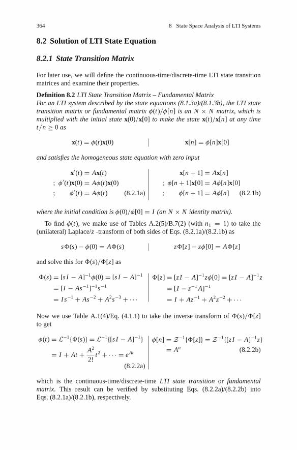
364 8 State Space Analysis of LTI Systems
8.2 Solution of LTI State Equation
8.2.1 State Transition Matrix
For later use, we will define the continuous-time/discrete-time LTI state transitionmatrices and examine their properties.
Definition 8.2 LTI State Transition Matrix – Fundamental MatrixFor an LTI system described by the state equations (8.1.3a)/(8.1.3b), the LTI statetransition matrix or fundamental matrix φ(t)/φ[n] is an N × N matrix, which ismultiplied with the initial state x(0)/x[0] to make the state x(t)/x[n] at any timet/n ≥ 0 as
x(t) = φ(t)x(0) x[n] = φ[n]x[0]
and satisfies the homogeneous state equation with zero input
x′(t) = Ax(t)
; φ′(t)x(0) = Aφ(t)x(0)
; φ′(t) = Aφ(t) (8.2.1a)
x[n + 1] = Ax[n]
; φ[n + 1]x[0] = Aφ[n]x[0]
; φ[n + 1] = Aφ[n] (8.2.1b)
where the initial condition is φ(0)/φ[0] = I (an N × N identity matrix).
To find φ(t), we make use of Tables A.2(5)/B.7(2) (with n1 = 1) to take the(unilateral) Laplace/z -transform of both sides of Eqs. (8.2.1a)/(8.2.1b) as
sΦ(s) − φ(0) = AΦ(s) zΦ[z] − zφ[0] = AΦ[z]
and solve this for Φ(s)/Φ[z] as
Φ(s) = [s I − A]−1φ(0) = [s I − A]−1
= [I − As−1]−1s−1
= I s−1 + As−2 + A2s−3 + · · ·
Φ[z] = [z I − A]−1zφ[0] = [z I − A]−1z
= [I − z−1 A]−1
= I + Az−1 + A2z−2 + · · ·
Now we use Table A.1(4)/Eq. (4.1.1) to take the inverse transform of Φ(s)/Φ[z]to get
φ(t) = L−1{Φ(s)} = L−1{[s I − A]−1}
= I + At + A2
2!t2 + · · · = eAt
(8.2.2a)
φ[n] = Z−1{Φ[z]} = Z−1{[z I − A]−1z}= An (8.2.2b)
which is the continuous-time/discrete-time LTI state transition or fundamentalmatrix. This result can be verified by substituting Eqs. (8.2.2a)/(8.2.2b) intoEqs. (8.2.1a)/(8.2.1b), respectively.

8.2 Solution of LTI State Equation 365
The LTI state transition matrices possess the following properties:<Properties of the LTI state transition matrix>
1) φ(t1)φ(t2) = φ(t1 + t2) ∀ t1, t22) φ(−t) = φ−1(t); φ(0) = I3) φ(t) = eAt is nonsingular ∀ t < ∞
1) φ[n1]φ[n2] = φ[n1 + n2] ∀ n1, n2
2) φ[−n] = φ−1[n]; φ[0] = I if φ[n]is nonsingular.
8.2.2 Transformed Solution
To solve the LTI state equations (8.1.3a)/(8.1.3b), we make use of Tables A.2(5)/B.7(2) (with n1 = 1) to take the (unilateral) Laplace/z -transform of both sidesand write
s X (s) − x(0) = AX (s) + BU (s)
; [s I − A]X (s) = x(0) + BU (s)
zX [z] − zx[0] = AX [z] + BU [z]
; [z I − A]X [z] = zx[0] + BU [z]
which can be solved for X (s)/X [z] as
X (s) = [s I − A]−1x(0)
+[s I − A]−1 BU (s) (8.2.3a)
X [z] = [z I − A]−1zx[0]
+[z I − A]−1 BU [z] (8.2.3b)
Now, we will find the inverse transform of this transformed solution:
x(t) = L−1{[s I − A]−1}x(0)
+ L−1{[s I − A]−1 BU (s)}(8.2.4a)
x[n] = Z−1{[z I − A]−1z}x[0]
+ Z−1{[z I − A]−1 BU [z]}(8.2.4b)
We can use Eq. (8.2.2), the convolution property, and the causality assumptionto write
L−1{[s I − A]−1} (8.2.2a)= eAt (8.2.5a) Z−1{[z I − A]−1z} (8.2.2b)= An (8.2.5b)
L−1{[s I − A]−1 BU (s)}B.7(4)= L−1{[s I − A]−1} ∗ L−1{BU (s)}
(8.2.5a)= eAt ∗ Bu(t)
(A.17)=∫ t
0eA(t−τ ) Bu(τ )dτ (8.2.6a)
Z−1{[z I − A]−1 BU [z]}B.7(4)= Z−1{[z I − A]−1} ∗ Z−1{BU [z]}
(8.2.5b)= An−1 ∗ Bu[n]
=∑n−1
m=0An−1−m Bu[m] (8.2.6b)
Substituting Eqs. (8.2.5) and (8.2.6) into Eq. (8.2.4) yields the solution of the LTIstate equation as
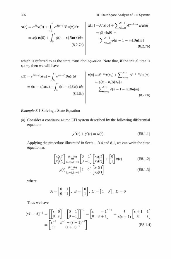
366 8 State Space Analysis of LTI Systems
x(t) = eAt x(0) +∫ t
0eA(t−τ ) Bu(τ )dτ
= φ(t)x(0) +∫ t
0φ(t − τ )Bu(τ )dτ
(8.2.7a)
x[n] =Anx[0] +∑n−1
m=0An−1−m Bu[m]
= φ[n]x[0]+∑n−1
m=0φ[n − 1 − m]Bu[m]
(8.2.7b)
which is referred to as the state transition equation. Note that, if the initial time ist0/n0, then we will have
x(t) = eA(t−t0)x(t0) +∫ t
t0
eA(t−τ ) Bu(τ )dτ
= φ(t − t0)x(t0) +∫ t
t0
φ(t − τ )Bu(τ )dτ
(8.2.8a)
x[n] =An−n0 x[n0] +∑n−1
m=n0An−1−m Bu[m]
= φ[n − n0]x[n0]+∑n−1
m=n0φ[n − 1 − m]Bu[m]
(8.2.8b)
Example 8.1 Solving a State Equation
(a) Consider a continuous-time LTI system described by the following differentialequation:
y′′(t) + y′(t) = u(t) (E8.1.1)
Applying the procedure illustrated in Sects. 1.3.4 and 8.1, we can write the stateequation as
[x ′
1(t)x ′
2(t)
](8.1.5a)=
a0=0,a1=1
[0 10 −1
] [x1(t)x2(t)
]+[
01
]u(t) (E8.1.2)
y(t)(8.1.6a)=
b0=1,b1=0
[1 0
] [x1(t)x2(t)
](E8.1.3)
where
A =[
0 10 −1
], B =
[01
], C = [
1 0], D = 0
Thus we have
[s I − A]−1 =[[
s 00 s
]−[
0 10 −1
]]−1
=[
s − 10 s + 1
]−1
= 1
s(s + 1)
[s + 1 1
0 s
]
=[
s−1 s−1 − (s + 1)−1
0 (s + 1)−1
](E8.1.4)

8.2 Solution of LTI State Equation 367
so that the state transition matrix is
φ(t)(8.2.2a)= L−1{[s I − A]−1} (E8.1.4)=
B.8(3),(6)
[1 1 − e−t
0 e−t
]for t ≥ 0 (E8.1.5)
Therefore, from Eq. (8.2.7a), we can write the solution of the state equation as
[x1(t)x2(t)
](8.2.7a)=(E8.1.5)
[1 1 − e−t
0 e−t
] [x1(0)x2(0)
]+∫ t
0
[1 − e−(t−τ )
e−(t−τ )
]u(τ )dτ for t ≥ 0
(E8.1.6)(b) Consider a discrete-time LTI system described by the following state equation:
[x1[n + 1]x2[n + 1]
]=[
1 1 − e−T
0 e−T
] [x1[n]x2[n]
]+[
T − 1 + e−T
1 − e−T
]u[n] (E8.1.7)
y[n] = [1 0
] [x1[n]x2[n]
](E8.1.8)
where
A =[
1 1 − e−T
0 e−T
], B =
[T − 1 + e−T
1 − e−T
], C = [
1 0], D = 0
For this system, we have
[z I − A]−1z =[[
z 00 z
]−[
1 1 − e−T
0 e−T
]]−1
z =[
z − 1 −1 + e−T
0 z − e−T
]−1
z
= z
(z − 1)(z − e−T )
[z − e−T 1 − e−T
0 z − 1
]
=[
zz−1
(1−e−T )z(z−1)(z−e−T )
0 zz−e−T
]=[
zz−1
zz−1 − z
z−e−T
0 zz−e−T
](E8.1.9)
so that the state transition matrix is
φ[n](8.2.2b)= Z−1{[z I − A]−1z} (E8.1.9)=
B.8(3),(6)
[1 1 − e−nT
0 e−nT
]for n ≥ 0 (E8.1.10)
as would be obtained from φ[n](8.2.2b)= An . Therefore, from Eq. (8.2.7b), we can
write the solution of the state equation as
[x1[n]x2[n]
](8.2.7b)=
(E8.1.10)
[1 1 − e−nT
0 e−nT
] [x1[0]x2[0]
]+
n−1∑m=0
[T − (1 − e−T )e−(n−1−m)T
(1 − e−T )e−(n−1−m)T
]u[m]
for n ≥ 0 (E8.1.11)
368 8 State Space Analysis of LTI Systems
8.2.3 Recursive Solution
The discrete-time state equation has a recursive form and therefore is well-suitedfor a digital computer, which can be programmed to perform the following compu-tation:
x[1] = Ax[0] + Bu[0]
x[2] = Ax[1] + Bu[1] = A2x[0] + ABu[0] + Bu[1]
x[3] = Ax[2] + Bu[2] = A3x[0] + A2 Bu[0] + ABu[1] + Bu[2] (8.2.9)
. . . . . . . . . . . . . . . . . . . . . . . . . . . . . . ..
x[n] = Anx[0] +∑n−1
m=0An−1−m Bu[m]
If the continuous-time state equation is somehow discretized, it can be solvedrecursively, too.
8.3 Transfer Function and Characteristic Equation
8.3.1 Transfer Function
Using the transformed solution (8.2.3) of the state equation, we can write thetransform of the output equation (8.1.4) with zero initial condition as
Y (s) = C X (s) + DU (s)(8.2.3a)=x(t)=0
C[s I − A]−1 BU (s) + DU (s)
(8.3.1a)
Y [z] = C X [z] + DU [z](8.2.3b)=x[n]=0
C[z I − A]−1 BU [z] + DU [z]
(8.3.1b)
Thus the transfer function matrix describing the input-output relationship turns outto be
G(s) = C[s I − A]−1 B + D (8.3.2a) G[z] = C[z I − A]−1 B + D (8.3.2b)
Taking the inverse transform of this transfer function matrix yields the impulseresponse matrix:
g(t) = Cφ(t)B + Dδ(t) (8.3.3a) g[n] = Cφ[n − 1]B + Dδ[n] (8.3.3b)

8.3 Transfer Function and Characteristic Equation 369
8.3.2 Characteristic Equation and Roots
Note that the transfer function matrix (8.3.2) can be written as
G(s) = CAdj [s I − A]
|s I − A| B + D (8.3.4a) G[z] = CAdj [z I − A]
|z I − A| B + D (8.3.4b)
where Adj[s I − A] denotes the adjoint, i.e., the transpose of the cofactor matrix.The characteristic equation of an LTI system is obtained by equating the denom-
inator of the transfer function to zero:
|s I − A| = 0 (8.3.5a) |z I − A| = 0 (8.3.5a)
Therefore, the roots of the characteristic equation are the eigenvalues of the matrix Aand are often called the characteristic roots of the system. The physical implicationof a characteristic root s0/z0 is that there will appear such terms as K es0t/K (z0)n inthe natural response of the system.
(cf.) The natural response means the output stemming from the initial condition,while the forced response means the output caused by the input.
Example 8.2 Transfer Function
(a) For the continuous-time LTI system described by Eq. (E8.1.2) in Example 8.1(a),we can use Eq. (8.3.2a) to find the transfer function
G(s)(8.3.2a)= C[s I − A]−1 B + D = [ 1 0 ]
[s −10 s + 1
]−1 [01
]
= [ 1 0 ]
s(s + 1)
[s + 1 1
0 s
] [01
]= 1
s(s + 1)(E8.2.1)
This could be obtained directly by taking the transform of the differential equa-tion (E8.1.1). We can equate the denominator of this transfer function with zeroto write the characteristic equation
|s I − A| = s(s + 1) = 0 (E8.2.2)
which has the roots s = 0 and s = −1 as the eigenvalues.(b) For the discrete-time LTI system described by Eq. (E8.1.7) in Example 8.1(b),
we can use Eq. (8.3.2b) to find the transfer function

370 8 State Space Analysis of LTI Systems
G[z](8.3.2b)= C[z I − A]−1 B + D = [ 1 0 ]
[z−1 −1 + e−T
0 z − e−T
]−1 [T − 1 + e−T
1 − e−T
]
= [ 1 0 ]
(z − 1)(z − e−T )
[z − e−T 1 − e−T
0 z − 1
] [T − 1 + e−T
1 − e−T
]
= (T − 1 + e−T )z + 1 − e−T − T e−T
(z − 1)(z − e−T )(E8.2.3)
We can equate the denominator with zero to write the characteristic equation
|z I − A| = (z − 1)(z − e−T ) = 0 (E8.2.4)
which has the roots z = 1 and z = e−T as the eigenvalues.
8.4 Discretization of Continuous-Time State Equation
In Chap. 6, we studied various discretzation methods that can be used for convertinga given s -transfer function or a differential equation into an ‘equivalent’ z -transferfunction or a difference equation. In this section, we will develop a technique todiscretize a continuous-time state equation into an ‘equivalent’ discrete-time stateequation.
8.4.1 State Equation Without Time Delay
Let us consider a continuous-time state equation
x′(t) = Ax(t) + Bu(t) (8.4.1)
y(t) = Cx(t) + Du(t) (8.4.2)
As shown in Sect. 8.2.2, the solution to these equations is given by Eq. (8.2.8a):
x(t) = φ(t − t0)x(t0) +∫ t
t0
φ(t − τ )Bu(τ )dτ (8.4.3)
To obtain an ‘equivalent’ discrete-time state equation, we write the state transitionequation for an interval of sampling period T from t0 = nT to t = (n + 1)T :
x((n + 1)T ) = φ(T )x(nT ) +∫ (n+1)T
nTφ(nT + T − τ )Bu(τ )dτ (8.4.4)
Assuming that the input is constant during each sampling interval, i.e., u(t) =u(nT ) = u[n] for nT ≤ t < (n + 1)T , we can rewrite this equation as

8.4 Discretization of Continuous-Time State Equation 371
x[n + 1] = φ(T )x[n] +∫ (n+1)T
nTφ(nT + T − τ )dτ Bu[n]
; x[n + 1] = ADx[n] + BDu[n] (8.4.5)
where we have let x(nT ) = x[n], u(nT ) = u[n], and
AD = φ(T ) = eAT (8.4.6a)
BD =∫ (n+1)T
nTφ(nT + T − τ )dτ B
nT +T −τ→σ= −∫ 0
Tφ(σ )dσ B =
∫ T
0φ(τ )dτ B
(8.4.6b)
We can get the discrete-time system matrices AD and BD by substituting the statetransition matrix (8.2.2a) into these Eqs. (8.4.6a) and (8.4.6b), which is cumbersomein general. As an alternative, it may be better to use a digital computer for evaluatingthem in the following way [F-1]:
AD(8.4.6a)= eAT (D.25)=
∞∑m=0
Am T m
m!= I + AT
∞∑m=0
Am T m
(m + 1)!= I + AT Ψ (8.4.7a)
BD =∫ T
0
∑∞m=0
Amτm
m!dτ B =
∑∞m=0
Am T m+1
(m + 1)!B = ΨT B (8.4.7b)
with
Ψ =∞∑
m=0
Am T m
(m + 1)!� I+ AT
2
(I + AT
3
(I + · · ·
(I + AT
N − 1
(I + AT
N
))· · ·
))(8.4.8)
Here, the infinite number of summations in Eq. (8.4.8) is truncated to some finitenumber N , which will be chosen in consideration of the desired accuracy andcomputation time.
Example 8.3 Discretization of a Continuous-Time State Equation
Consider a continuous-time LTI system described by Eqs. (E8.1.2) and (E8.1.3)in Example 8.1(a), where the state transition matrix is given by Eq. (E8.1.5) as
φ(t)(8.2.2a)= L−1{[s I − A]−1} (E8.1.5)=
[1 1 − e−t
0 e−t
]for t ≥ 0 (E8.3.1)

372 8 State Space Analysis of LTI Systems
(a) Find the discretized state equation.We can use Eqs. (8.4.6a) and (8.4.6b) to get
AD(8.4.6a)= φ(T ) =
[1 1 − e−T
0 e−T
](E8.3.2)
BD(8.4.6b)=
∫ T
0φ(τ )dτ B =
[τ τ + e−τ
0 −e−τ
]∣∣∣∣T
0
[01
]=[
T T + e−T − 10 −e−T + 1
] [01
]
=[
T + e−T − 11 − e−T
](E8.3.3)
so that the discretized state equation can be obtained as
[x1[n + 1]x2[n + 1]
](8.4.5)=
[1 1 − e−T
0 e−T
] [x1[n]x2[n]
]+[
T + e−T − 11 − e−T
]u[n] (E8.3.4)
%sig08e03.mclear, clfsyms s zNs=1; Ds=[1 1 0]; Gs=tf(Ns,Ds); % Analog transfer function[A,B,C,D]=tf2ss(Ns,Ds) % Transfer function to state equationN=size(A,2); % the dimension of the system% The numerator/denominator of transfer function (8.3.2a)[Ns,Ds]=ss2tf(A,B,C,D)Gs1= C*(s*eye(N)-A)ˆ-1*B + D; pretty(Gs1) % Eq.(8.3.2a)T=0.1; NT=101; t=[0:NT-1]*T;% To find the response to step input applied to the 1st input terminal[y,x,tt]=step(A,B,C,D,1,t);syms s t %for symbolic solution of the state eq.A=[0 1;0 -1]; B=[0 1]’; % Eq.(E8.1.2)x0=[0 0]’; % zero initial condition% Laplace transform solutionXs=(s*eye(N)-A)ˆ-1*(x0+B/s) % Eq.(8.2.3a)% Inverse Laplace transformfor n=1:N, xt(n)=ilaplace(Xs(n)), endfor n=1:length(tt)
t=tt(n); y1(n)=eval(xt(1)); % Eq.(E8.1.3) with C=[1 0]end% To solve the differential equation directlyx=dsolve(’Dx1=x2,Dx2=-x2+1’,’x1(0)=0,x2(0)=0’); % Eq.(E8.1.2)t=tt; y2= eval(x.x1); % Eq.(E8.1.3) with C=[1 0]plot(tt,y,’k’, tt,y1,’b’, tt,y2,’r’)% DiscretizationA=[0 1;0 -1]; B=[0 1]’; C=[1 0]; D=0; % Eq.(E8.1.2)[Ad,Bd,Cd,Dd]=c2dm(A,B,C,D,T,’zoh’) % Discretized state equation[Ad1,Bd1]=c2d steq(A,B,T) % Eq.(8.4.7a,b)e T=exp(-T); Ad2=[1 1-e T; 0 e T], Bd2=[T+e T-1; 1-e T] % Eq.(E8.3.4)% The numerator/denominator of transfer function (8.3.2b)[Nz,Dz]=ss2tf(Ad,Bd,Cd,Dd) % Eq.(8.3.2b) to (E8.2.3) or (E8.3.5)Nz1=[T-1+e T 1-e T-T*e T], Dz1=[1 -1-e T e T]%Gz1= Cd*(z*eye(N)-Ad)ˆ-1*Bd + Dd, pretty(Gz1)% The z.o.h. equivalent of the analog transfer function

8.4 Discretization of Continuous-Time State Equation 373
Gz zoh=c2d(Gs,T,’zoh’);[Bd zoh,Ad zoh]=tfdata(Gz zoh,’v’) % Eq.(E8.3.7)% To find the response to step input applied to the 1st input terminalyd=dstep(Ad,Bd,Cd,Dd,1,NT);hold on, stairs(tt,yd)
function [Ad,Bd]=c2d steq(A,B,T,N)if nargin<4, N=100; endI= eye(size(A,2)); PSI= I;for m=N:-1:1, PSI= I +A*PSI*T/(m+1); end % Eq.(8.4.8)Ad= I +A*T*PSI; Bd= PSI*T*B; % Eq.(8.4.7a,b)
Note that this is identical to Eq. (E8.1.7) in Example 8.1(b) and the trans-fer function of the system was computed via Eq. (8.3.2b) as Eq. (E8.2.3) inExample 8.2:
G D[z] = (T − 1 + e−T )z + 1 − e−T − T e−T
(z − 1)(z − e−T )(E8.3.5)
(b) Find the transfer function for the z.o.h. (step-invariant) equivalent of the continuous-time system.Noting from Eq. (E8.2.1) that the transfer function of the continuous-timesystem is
G(s)(E8.2.1)= 1
s(s + 1), (E8.3.6)
we can use Eq. (6.2.5) to get
Gstep[z](6.2.5)= (1 − z−1)Z
{L−1
{1
sG(s)
}∣∣∣∣t=nT
}(E8.3.6)= z − 1
zZ{L−1
{1
s2(s + 1)
}}PFE= z − 1
zZ{L−1
{1
s2+ −1
s+ 1
s + 1
}}B.8(3),(4)&(6)= z − 1
z
(T z
(z − 1)2− z
z − 1+ z
z − e−T
)= T
z − 1− 1 + z − 1
z − e−T
= (T − 1 + e−T )z + 1 − e−T − T e−T
(z − 1)(z − e−T )(E8.3.7)
This is the same as the transfer function of the system described by the dis-cretized state equation (E8.3.4) and output equation (E8.1.8). It is because wehave assumed that the input is constant during each sampling period in dis-cretizing the state equation as if a S/H (sampler and zero-order-hold) devicewere installed at the input stage.Interested readers are invited to run the above program “sig08e03.m”, check thevalidity of the above results, and see how the MATLAB commands can be usedto discretize a continuous-time state equation.
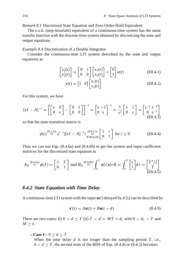
374 8 State Space Analysis of LTI Systems
Remark 8.1 Discretized State Equation and Zero-Order-Hold EquivalentThe z.o.h. (step-invariant) equivalent of a continuous-time system has the same
transfer function with the discrete-time system obtained by discretizing the state andoutput equations.
Example 8.4 Discretization of a Double IntegratorConsider the continuous-time LTI system described by the state and output
equations as
[x ′
1(t)x ′
2(t)
]=[
0 10 0
] [x1(t)x2(t)
]+[
01
]u(t) (E8.4.1)
y(t) = [1 0
] [x1(t)x2(t)
](E8.4.2)
For this system, we have
[s I − A]−1 =[[
s 00 s
]−[
0 10 0
]]−1
=[
s −10 s
]−1
= 1
s2
[s 10 s
]=[
s−1 s−2
0 s−1
](E8.4.3)
so that the state transition matrix is
φ(t)(8.2.2a)= L−1{[s I − A]−1} (E8.4.3)=
B.8(3),(4)
[1 t0 1
]for t ≥ 0 (E8.4.4)
Thus we can use Eqs. (8.4.6a) and (8.4.6b) to get the system and input coefficientmatrices for the discretized state equation as
AD(8.4.6a)= φ(T ) =
[1 T0 1
]and BD
(8.4.6b)=∫ T
0φ(τ )dτ B =
∫ T
0
[τ
1
]dτ =
[T 2/2
T
](E8.4.5)
8.4.2 State Equation with Time Delay
A continuous-time LTI system with the input u(t) delayed by d [s] can be described by
x′(t) = Ax(t) + Bu(t − d) (8.4.9)
There are two cases: (i) 0 < d ≤ T (ii) T < d = MT + d1 with 0 < d1 < T andM ≥ 1.
<Case I> 0 ≤ d ≤ TWhen the time delay d is not longer than the sampling period T , i.e.,0 < d ≤ T , the second term of the RHS of Eqs. (8.4.4) or (8.4.5) becomes

8.4 Discretization of Continuous-Time State Equation 375
∫ (n+1)T
nTφ(nT + T − τ )Bu(τ − d)dτ
=∫ nT +d
nTφ(nT + T − σ )dσ Bu(nT − T )
+∫ nT +T
nT +dφ(nT + T − σ )dσ Bu(nT ) (8.4.10)
where the input signal u(t) is assumed to be constant over each samplinginterval. Thus Eq. (8.4.5) becomes
x[n + 1] = ADx[n] + BD1u[n − 1] + BD0u[n] (8.4.11)
where
AD(8.4.6a)= φ(T ) = eAT (8.4.12a)
BD1(8.4.6b)=
∫ nT +d
nTφ(nT + T − σ )dσ B
nT +T −σ→τ= −∫ 0
dφ(T − d + τ )dτ B = φ(T − d)
∫ d
0φ(τ )dτ B
(8.4.12b)
BD0(8.4.6b)=
∫ nT +T
nT +dφ(nT + T − σ )dσ B
nT +T −σ→τ= −∫ 0
T −dφ(τ )dτ B =
∫ T −d
0φ(τ )dτ B (8.4.12c)
This can be written in the form of state equation as
[x[n + 1]
u[n]
]=[
AD BD1
O O
] [x[n]
u[n − 1]
]+[
BD0
I
]u[n] (8.4.13)
where K extra state variables u[n − 1] representing the past input values areintroduced to augment the state vector.
<Case II> T < d = MT + d1 with 0 < d1 < T and M ≥ 1When the time delay d is longer than the sampling period T so that d =MT + d1 with 0 < d1 < T and some integer M ≥ 1, Eq. (8.4.11) becomes
x[n + 1] = ADx[n] + BD1u[n − M − 1] + BD0u[n − M] (8.4.14)
where the matrices AD, BD1, and BD0 are as defined by Eqs. (8.4.12a,b,c).This can be written in the form of state equation as

376 8 State Space Analysis of LTI Systems
⎡⎢⎢⎢⎢⎢⎢⎣
x[n + 1]u[n − M]
••
u[n − 1]u[n]
⎤⎥⎥⎥⎥⎥⎥⎦
=
⎡⎢⎢⎢⎢⎢⎢⎣
AD BD1 BD0 O · · · OO O I O · · · O• • • • · · · •• • • • · · · •O O O O · · · IO O O O · · · O
⎤⎥⎥⎥⎥⎥⎥⎦
⎡⎢⎢⎢⎢⎢⎢⎣
x[n]u[n − M − 1]
••
u[n − 2]u[n − 1]
⎤⎥⎥⎥⎥⎥⎥⎦
+
⎡⎢⎢⎢⎢⎢⎢⎣
OO••OI
⎤⎥⎥⎥⎥⎥⎥⎦
u[n]
(8.4.15)where (M +1)K extra state variables {u[n −1], u[n −2], · · · , u[n − M −1]}representing the past input values are introduced.
u(t )
u(t – d )
nT – T nT + TnT
nT – T
d
nT + TnT
t
t
Fig. 8.1 Delayed input signal by d
Example 8.5 Discretization of a Double Integrator with Time DelayConsider the double integrator dealt with in Example 8.4, where the input is
delayed by d (0 < d < T ). With the state transition matrix φ(t) given byEq. (E8.4.4), we use Eq. (8.4.12) to get the discrete-time system matrices as
AD = φ(T ) =[
1 T0 1
](E8.5.1)
BD1 = φ(T − d)∫ d
0φ(τ )dτ B =
[1 T − d0 1
] [d2/2
d
]=[
d(T − d/2)d
](E8.5.2)
BD0 =∫ T −d
0φ(τ )dτ B =
[τ 2/2
τ
]∣∣∣∣T −d
0
=[
(T − d)2/2T − d
](E8.5.3)
8.5 Various State Space Description – Similarity Transformation
As can be seen in Sect. 1.3.4, we could construct many state diagrams for a giventransfer function and each of them can be represented by a state equation. Thisimplies that there is no unique state space model for a certain system.

8.5 Various State Space Description – Similarity Transformation 377
As a matter of fact, we can use similarity transformation to derive any numberof different state equations, all of which are equivalent in terms of the input-outputrelationship. Consider the state and output equation of an LTI system as
State equation:
x′(t) = Ax(t) + Bu(t) (8.5.1a)
Output equation:
y(t) = Cx(t) + Du(t) (8.5.2a)
x[n + 1] = Ax[n] + Bu[n] (8.5.1b)
y[n] = Cx[n] + Du[n] (8.5.2b)
With a nonsingular transformation matrix P and a new state vector w(t)/w[n], wesubstitute
x(t) = P w(t) (8.5.3a) x[n] = P w[n] (8.5.3b)
into Eqs. (8.5.1) and (8.5.2) to write
w′(t) = P−1 APw(t) + P−1 Bu(t)
y(t) = C Pw(t) + Du(t)
w[n + 1] = P−1 APw[n] + P−1 Bu[n]
y[n] = C Pw[n] + Du[n]
This can be written as another set of state and output equations:
w′(t) = Apw(t) + Bpu(t) (8.5.4a)
y(t) = C pw(t) + Dpu(t) (8.5.5a)
w[n +1] = Apw[n]+ Bpu[n] (8.5.4b)
y[n] = Cpw[n] + Dpu[n] (8.5.5b)
where
Ap = P−1 AP, Bp = P−1 B, C p = C P, and Dp = D (8.5.6)
Remark 8.2 Similarity Transformation – Equivalence Transformation
(1) Note that, with different nonsingular matrices P , we could obtain different setof state and output equations as many as we want.
(2) Transfer function, characteristic equation, and eigenvalues are not changedunder similarity transformation:
|s I − Ap|=|s I −P−1 AP|=|P−1s I P−P−1 AP|=|P−1||s I − A||P|=|s I − A|(8.5.7)
(3) The determinant/trace of Ap is the same as that of A, since the determinant/traceof a matrix is equal to the product/sum of the eigenvalues. Especially if a systemhas distinct characteristic values, we may derive a state equation with a diagonalsystem matrix having the characteristic values on its diagonal, which is referredto as the Jordan canonical or normal form.
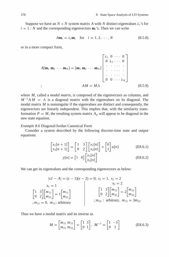
378 8 State Space Analysis of LTI Systems
Suppose we have an N × N system matrix A with N distinct eigenvalues λi ’s fori = 1 : N and the corresponding eigenvectors mi ’s. Then we can write
Ami = λi mi for i = 1, 2, · · · , N (8.5.8)
or in a more compact form,
A[m1 m2 · · · mN ] = [m1 m2 · · · mN ]
⎡⎢⎢⎢⎢⎢⎢⎣
λ1 0 · · · 00 λ2 · · · 0· · · · · ·· · · · · ·· · · · · ·0 0 · · · λN
⎤⎥⎥⎥⎥⎥⎥⎦
; AM = MΛ (8.5.9)
where M , called a modal matrix, is composed of the eigenvectors as columns, andM−1 A M = Λ is a diagonal matrix with the eigenvalues on its diagonal. Themodal matrix M is nonsingular if the eigenvalues are distinct and consequently, theeigenvectors are linearly independent. This implies that, with the similarity trans-formation P = M , the resulting system matrix Ap will appear to be diagonal in thenew state equation.
Example 8.6 Diagonal/Jordan Canonical FormConsider a system described by the following discrete-time state and output
equations:
[x1[n + 1]x2[n + 1]
]=[
1 30 2
] [x1[n]x2[n]
]+[
01
]u[n] (E8.6.1)
y[n] = [1 0
] [x1[n]x2[n]
](E8.6.2)
We can get its eigenvalues and the corresponding eigenvectors as below:
|s I − A| = (s − 1)(s − 2) = 0; s1 = 1, s2 = 2
s1 = 1[1 30 2
][m11
m21
]= 1
[m11
m21
]; m21 = 0, m11: arbitrary
s2 = 2[1 30 2
][m12
m22
]= 2
[m12
m22
]; m22 : arbitrary, m12 = 3m22
Thus we have a modal matrix and its inverse as
M =[
m11 m12
m21 m22
]=[
1 30 1
], M−1 =
[1 −30 1
](E8.6.3)
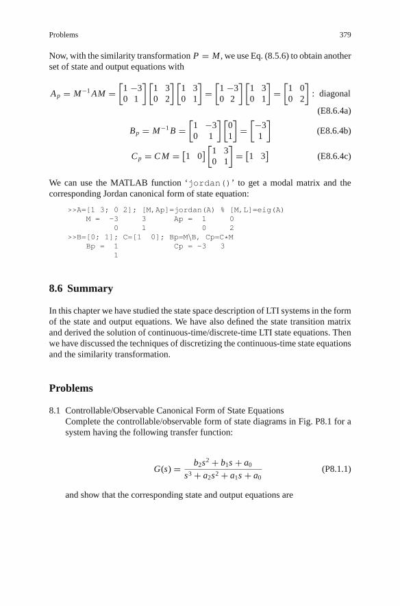
Problems 379
Now, with the similarity transformation P = M , we use Eq. (8.5.6) to obtain anotherset of state and output equations with
Ap = M−1 AM =[
1 −30 1
] [1 30 2
] [1 30 1
]=[
1 −30 2
] [1 30 1
]=[
1 00 2
]: diagonal
(E8.6.4a)
Bp = M−1 B =[
1 −30 1
] [01
]=[−3
1
](E8.6.4b)
Cp = C M = [1 0
] [1 30 1
]= [
1 3]
(E8.6.4c)
We can use the MATLAB function ‘jordan()’ to get a modal matrix and thecorresponding Jordan canonical form of state equation:
>>A=[1 3; 0 2]; [M,Ap]=jordan(A) % [M,L]=eig(A)M = -3 3 Ap = 1 0
0 1 0 2>>B=[0; 1]; C=[1 0]; Bp=M\B, Cp=C*M
Bp = 1 Cp = -3 31
8.6 Summary
In this chapter we have studied the state space description of LTI systems in the formof the state and output equations. We have also defined the state transition matrixand derived the solution of continuous-time/discrete-time LTI state equations. Thenwe have discussed the techniques of discretizing the continuous-time state equationsand the similarity transformation.
Problems
8.1 Controllable/Observable Canonical Form of State EquationsComplete the controllable/observable form of state diagrams in Fig. P8.1 for asystem having the following transfer function:
G(s) = b2s2 + b1s + a0
s3 + a2s2 + a1s + a0(P8.1.1)
and show that the corresponding state and output equations are

380 8 State Space Analysis of LTI Systems
y (t )Y (s )
x3(t )
x2(t )
x1(t )
x1(t )
(a) Controllable canonical form (b) Observable canonical form–a0
–a2b2
b1–a1
b0
x3(t )′
x3(t )′
x2(t )′
x1(t )′
x2(t )
x1(t )
x3(t )
x2(t )′
x1(t )′
u(t )U(s )
s–1 s–1
s–1
s–1
s–1
s–1
u(t )U(s )
y (t )Y (s )
Fig. P8.1 Controllable/observable canonical state diagrams for the transfer function (P8.1.1)
⎡⎣x ′
1(t)x ′
2(t)x ′
3(t)
⎤⎦ =
⎡⎣ 0 1 0
0 0 1−a0 −a1 −a2
⎤⎦⎡⎣x1(t)
x2(t)x3(t)
⎤⎦
+⎡⎣0
01
⎤⎦ u(t) (P8.1.2a)
⎡⎣x ′
1(t)x ′
2(t)x ′
3(t)
⎤⎦ =
⎡⎣0 0 −a0
1 0 −a1
0 1 −a2
⎤⎦⎡⎣x1(t)
x2(t)x3(t)
⎤⎦
+⎡⎣b0
b1
b2
⎤⎦ u(t) (P8.1.2b)
y(t) = [b0 b1 b2
]⎡⎣x1(t)x2(t)x3(t)
⎤⎦
(P8.1.3a)
y(t) = [0 0 1
]⎡⎣x1(t)x2(t)x3(t)
⎤⎦
(P8.1.3b)
8.2 Controllable/Observable Canonical Form of State EquationsConsider a system having the following transfer function:
G(s) = Y (s)
U (s)= 4(s + 3)
2s2 + 6s + 4(P8.2.1)
(a) Write the controllable/observable form of state and output equations andfind the state transition matrices.
(b) Show that the step response is
y(t) = (3 − 4e−t + e−2t )us(t) (P8.2.2)
8.3 State Transition MatrixFind the state transition matrix φ(t) = eAt for a state equation having thefollowing system matrix:
A =[λ 10 λ
](P8.3.1)

Problems 381
8.4 State Diagram and State Equation
(a) Show that the state and output equations for the state diagram of Fig. 1.20(a)are ⎡
⎢⎢⎣x1[n + 1]x2[n + 1]x3[n + 1]x4[n + 1]
⎤⎥⎥⎦ =
⎡⎢⎢⎣
0 1 0 0−a0 −a1 b0 b1
0 0 0 10 0 0 0
⎤⎥⎥⎦⎡⎢⎢⎣
x1[n]x2[n]x3[n]x4[n]
⎤⎥⎥⎦ +
⎡⎢⎢⎣
0001
⎤⎥⎥⎦ u[n] (P8.4.1)
y[n] = [−a0 −a1 b0 b1]⎡⎢⎢⎣
x1[n]x2[n]x3[n]x4[n]
⎤⎥⎥⎦ (P8.4.2)
(b) Use Eq. (8.3.2b) to find the transfer function of the system described by theabove state equation.
8.5 Discretization of a Continuous-Time State EquationConsider a system described by the following state and output equations:
[x ′
1(t)x ′
2(t)
]=[
0 10 −2
] [x1(t)x2(t)
]+[
01
]u(t) (P8.5.1)
y(t) = [1 0
] [x1(t)x2(t)
](P8.5.2)
(a) Use Eq. (8.3.2a) to find the transfer function G(s) of this continuous-timesystem.
(b) Discretize the above state equation and then use Eq. (8.3.2b) to find thetransfer function G D[z] of the discretized system. Compare G D[z] with thez.o.h. equivalent of G(s).
8.6 Discretization of a Continuous-Time State EquationNote that for an oscillator having the transfer function
G(s) = ω2
s2 + ω2(P8.6.1)
we can write the following state and output equations:
[x ′
1(t)x ′
2(t)
]=[
0 ω
ω 0
] [x1(t)x2(t)
]+[
0ω
]u(t) (P8.6.2)
y(t) = [1 0
] [x1(t)x2(t)
](P8.6.3)
(a) Use Eq. (8.3.2a) to find the transfer function G(s) of this continuous-timesystem.
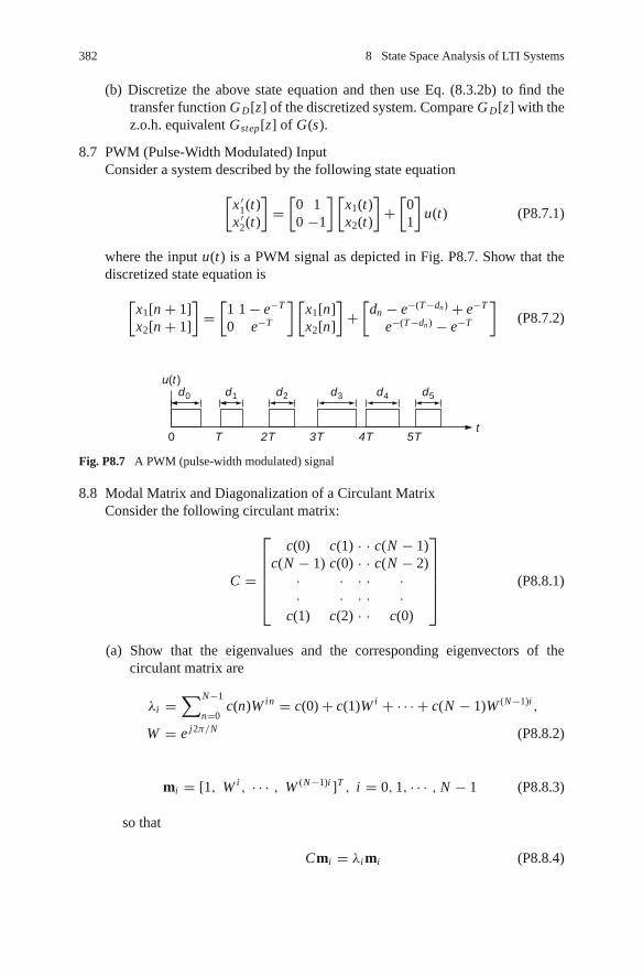
382 8 State Space Analysis of LTI Systems
(b) Discretize the above state equation and then use Eq. (8.3.2b) to find thetransfer function G D[z] of the discretized system. Compare G D[z] with thez.o.h. equivalent Gstep[z] of G(s).
8.7 PWM (Pulse-Width Modulated) InputConsider a system described by the following state equation
[x ′
1(t)x ′
2(t)
]=[
0 10 −1
] [x1(t)x2(t)
]+[
01
]u(t) (P8.7.1)
where the input u(t) is a PWM signal as depicted in Fig. P8.7. Show that thediscretized state equation is
[x1[n + 1]x2[n + 1]
]=[
1 1 − e−T
0 e−T
] [x1[n]x2[n]
]+[
dn − e−(T −dn ) + e−T
e−(T −dn ) − e−T
](P8.7.2)
d0
0 T 2T 3T 4T 5Tt
d1
u(t )d2 d3 d4 d5
Fig. P8.7 A PWM (pulse-width modulated) signal
8.8 Modal Matrix and Diagonalization of a Circulant MatrixConsider the following circulant matrix:
C =
⎡⎢⎢⎢⎢⎣
c(0) c(1) · · c(N − 1)c(N − 1) c(0) · · c(N − 2)
· · · · ·· · · · ·
c(1) c(2) · · c(0)
⎤⎥⎥⎥⎥⎦ (P8.8.1)
(a) Show that the eigenvalues and the corresponding eigenvectors of thecirculant matrix are
λi =∑N−1
n=0c(n)W in = c(0) + c(1)W i + · · · + c(N − 1)W (N−1)i ,
W = e j2π/N (P8.8.2)
mi = [1, W i , · · · , W (N−1)i ]T , i = 0, 1, · · · , N − 1 (P8.8.3)
so that
Cmi = λi mi (P8.8.4)

Problems 383
(b) Note that a modal matrix consisting of the eigenvectors can be written as
M = 1√N
[m0, m1, · · · , mN−1] = 1√N
⎡⎢⎢⎢⎢⎣
1 1 · · 11 W 1 · · W N−1
· · · · ·· · · · ·1 W N−1 · · W (N−1)2
⎤⎥⎥⎥⎥⎦
(P8.8.5)Show that the inverse of the modal matrix is
M−1 =
⎡⎢⎢⎢⎢⎣
1 1 · · 11 W −1 · · W −(N−1)
· · · · ·· · · · ·1 W −(N−1) · · W −(N−1)2
⎤⎥⎥⎥⎥⎦ = M∗ (Conjugate transpose) (P8.8.6)
(c) With the matrix dimension N = 4, diagonalize the circulant matrix C by thesimilarity transformation. For reference, you can run the followingprogram “sig08p 08.m”.
%sig08p 08.mclear, clfsyms c0 c1 c2 c3C=[c0 c1 c2 c3; c3 c0 c1 c2; c2 c3 c0 c1; c1 c2 c3 c0];[M,L]=jordan(C) % [M,L]=eig(C)M*M’

Appendix AThe Laplace Transform
The Laplace transform was discovered originally by Leonhard Euler (1707–1783),the great 18th-century Swiss mathematician and physicist, but is named in honor ofa French mathematician and astronomer Pierre-Simon Laplace (1749–1827), whoused the transform in his work on probability theory. He was such a genius notonly in mathematics that the great mathematician Simeon Poisson (1781–1840)labeled him the Isaac Newton of France, but also in politics that he could serve threeregimes in revolutionary France – the republic, the empire of Napoleon, and theBourbon restoration, having been bestowed a count from Napoleon and a marquisfrom Louis XVIII.
The Laplace transform is a very useful tool in solving differential equations andmuch further, it plays an important role in dealing with linear time-invariant systems.
A.1 Definition of the Laplace Transform
The (unilateral or one-sided) Laplace transform is defined for a function x(t) of areal variable t (often meaning the time) as
X (s) = L{x(t)} =∫ ∞
0−x(t)e−st dt (A.1)
where s is a complex variable, the lower limit, t−, of the integration interval is theinstant just before t = 0, and x(t) is often assumed to be causal in the sense that itis zero for all t < 0.
A.2 Examples of the Laplace Transform
A.2.1 Laplace Transform of the Unit Step Function
The unit step function is defined as
385

386 Appendix A
(a) Unit step function (b) Rectangular pulse (c) Unit impulse function0 0 0
t
rT (t )
= =lim rT (t ) (us(t +T→0
T→0
δ (t )
δ (t )T
T1
t t
us(t )lim
T→0lim
T1
2T
2T d
dt) – us (t – )) = us(t )
Fig. A.1 Unit step, rectangular pulse, and unit impulse functions
us(t) ={
1 for t ≥ 0
0 for t < 0(A.2)
which is depicted in Fig. A.1(a). We can use Eq. (A.1) to obtain the Laplacetransform of the unit step function as
L{us(t)} (A.1)=∫ ∞
0us(t)e−st dt
(A.2)=∫ ∞
0e−st dt
(D.33)= 1
−se−st
∣∣∞0 = 1
−s(0 − 1) = 1
s
This Laplace transform pair is denoted by
us(t)L←→ 1
s(A.3)
A.2.2 Laplace Transform of the Unit Impulse Function
The unit impulse function can be defined to be the limit of a rectangular pulse func-tion rT (t) with the pulsewidth T → 0 (converging to zero) or simply, the timederivative of the unit step function as
δ(t) = limT →0
rT (t) = limT →0
1
T
(us
(t + T
2
)− us
(t − T
2
))= d
dtus(t) (A.4)
which is depicted in Fig. A.1(c). We can use Eq. (A.1) to obtain the Laplacetransform of the unit impulse function as
L{δ(t)} =∫ ∞
0−δ(t)e−st dt = 1
This Laplace transform pair is denoted by
δ(t)L←→ 1 (A.5)

Appendix A 387
A.2.3 Laplace Transform of the Ramp Function
The Laplace transform of the unit ramp function tus(t) is obtained as
L{tus(t)} (A.1)=∫ ∞
0tus(t)e−st dt
(A.2)=∫ ∞
0te−st dt
(D.36)= t
−se−st
∣∣∞0 + 1
s
∫ ∞
0e−st dt
(D.33)= 1
s2
This Laplace transform pair is denoted by
tus(t)L←→ 1
s2(A.6)
A.2.4 Laplace Transform of the Exponential Function
The Laplace transform of the exponential function e−at us(t) is obtained as
L{e−at us(t)} (A.1)=∫ ∞
0e−at us(t)e−st dt
(A.2)=∫ ∞
0e−at e−st dt =
∫ ∞
0e−(s+a)t dt
(D.33)= 1
s + a
This Laplace transform pair is denoted by
e−at us(t)L←→ 1
s + a(A.7)
A.2.5 Laplace Transform of the Complex Exponential Function
Substituting σ + jω for a into (A.7) yields the Laplace transform of the complexexponential function as
e−(σ+ jω)t us(t)(D.20)= e−σ t (cos ωt − j sin ωt)us(t)
L←→1
s + σ + jω= s + σ
(s + σ )2 + ω2− j
ω
(s + σ )2 + ω2
e−σ t cos ωt us(t)L←→ s + σ
(s + σ )2 + ω2(A.8)
e−σ t sin ωt us(t)L←→ ω
(s + σ )2 + ω2(A.9)
A.3 Properties of the Laplace Transform
Let the Laplace transforms of two functions x(t) and y(t) be X (s) and Y (s),respectively.

388 Appendix A
A.3.1 Linearity
The Laplace transform of a linear combination of x(t) and y(t) can be written as
α x(t) + βy(t)L←→αX (s) + βY (s) (A.10)
A.3.2 Time Differentiation
The Laplace transform of the derivative of x(t) w.r.t. t can be written as
x ′(t)L←→ s X (s) − x(0) (A.11)
Proof
L{x ′(t)} (A.1)=∫ ∞
0
dx
dte−st
dt(D.36)= x(t)e−st
∣∣∞0 −(−s)
∫ ∞
0x(t)e−st dt
(A.1)= s X (s)−x(0)
Repetitive application of this time differentiation property yields the Laplace trans-form of n th-order derivative of x(t) w.r.t. t as
x (n)(t)L←→ sn X (s) − sn−1x(0) − sn−2x ′(0) − · · · − x (n−1)(0) (A.12)
A.3.3 Time Integration
The Laplace transform of the integral of x(t) w.r.t. t can be written as
∫ t
−∞x(τ )dτ
L←→ 1
sX (s) + 1
s
∫ 0
−∞x(τ )dτ (A.13)
This can be derived by substituting∫ t−∞ x(τ )dτ and x(t) for x(t) and x ′(t) into
Eq. (A.11) as
x(t)L←→ X (s) = sL
{∫ t
∞x(τ )dτ
}−∫ 0
−∞x(τ )dτ
Repetitive application of this time integration property yields the Laplace trans-form of n th-order integral of x(t) w.r.t. t as
∫ t
−∞
∫ t
−∞· ·∫ t
−∞x(τ )dτ n L←→ s−n X (s) + s−n
∫ 0
−∞x(τ )dτ + · · · +
∫ 0
−∞
∫ 0
−∞· ·∫ 0
−∞x(τ )dτ n
(A.14)

Appendix A 389
A.3.4 Time Shifting – Real Translation
The Laplace transform of a delayed function x(t) can be obtained as follows.
L {x(t − t1)} (A.1)=∫ t1
−∞x(t − t1)e−st dτ +
∫ ∞
t1
x(t − t1)e−st dτ
t−t1=τ= e−st1
∫ 0
−t1
x(τ )e−sτ dτ + e−st1
∫ ∞
0x(τ )e−sτ dτ ;
x(t − t1), t1 > 0L←→ e−st1
{X (s) +
∫ 0
−t1
x(τ )e−sτ dτ
}if x(t)=0 ∀ t<0→ e−s t1 X (s)
(A.15)
(a)0 (b)t
τ = t τ = tτ τ
t
Fig. A.2 Switching the order of two integrations for double integral
A.3.5 Frequency Shifting – Complex Translation
es1t x(t)L←→ X (s − s1) (A.16)
A.3.6 Real Convolution
The (real) convolution of two (causal) functions g(t) and x(t) is defined as
g(t) ∗ x(t) =∫ ∞
−∞g (τ ) x (t − τ ) dτ
if g(t)=0 and x(t)=0 ∀ t<0=causality
∫ t
0g (τ ) x (t − τ ) dτ
(A.17)
The Laplace transform of the convolution y(t) = g(t) ∗ x(t) turns out to be theproduct of the Laplace transforms of the two functions as
y(t) = g(t) ∗ x(t)L←→ Y (s) = G(s)X (s) (A.18)

390 Appendix A
Proof
L {g(t) ∗ x(t)} (A.1)=∫ ∞
0g(t) ∗ x(t)e−st dt
(A.17)=∫ ∞
0
{∫ t
0g(τ )x(t − τ )dτ
}e−st dt
Fig.A.2=∫ ∞
0g(τ )e−sτ
∫ ∞
τ
x(t − τ )e−s(t−τ )dt dτ
(t−τ=v)=∫ ∞
0g(τ )e−sτ
{∫ ∞
0x(v)e−svdv
}dτ
(A.1)=∫ ∞
0g(τ )e−sτ dτ X (s)
(A.1)= G (s) X (s)
This property is used to describe the input-output relationship of a linear time-invariant (LTI) system which has the input x(t), the impulse function g(t), andthe output y(t), where the Laplace transform of the impulse function, i.e., G(s) =L{g(t)}, is referred to as the system function or transfer function of the system.
A.3.7 Partial Differentiation
Given the Laplace transform of a function having a parameter a, that is L{x(t, a)} =X (s, a), the Laplace transform of the derivative of the parameterized function x(t, a)w.r.t. a equals the derivative of its Laplace transform X (s, a) w.r.t. a.
∂
∂ax(t, a)
L←→ ∂
∂aX (s, a) (A.19)
A.3.8 Complex Differentiation
The Laplace transform of −t x(t) equals the derivative of L{x(t)} = X (s) w.r.t. s.
t x(t)L←→− d
dsX (s) (A.20)
This can be derived by differentiating Eq. (A.1) w.r.t. s.
Example A.1 Applying Partial/Complex Differentiation PropertyTo find the Laplace transform of t e−at us(t), we differentiate Eq. (A.7) w.r.t. a
and multiply the result by −1 to get
t e−at us(t)L←→ 1
(s + a)2(A.21)

Appendix A 391
Multiplying t by the left-hand side (LHS) and applying the complex differentia-tion property (A.20) repetitively, we get
t2e−at us(t)L←→ 2!
(s + a)3(A.22)
. . . . . . . . . . . . . . . . . . . . . . . . . . .
tme−at us(t)L←→ m!
(s + a)m+1(A.23)
A.3.9 Initial Value Theorem
We can get the initial value of x(t) from its Laplace transform L{x(t)} = X (s) asfollows.
x(0) = lims→∞ s X (s) (A.24)
This can be derived by substituting s = ∞ into the time differentiation property(A.11) as
lims→∞ s X (s) − x(0)
(A.11)= lims→∞L
{x ′(t)
} (A.1)= lims→∞
∫ ∞
0x ′(t)e−st dt = 0
A.3.10 Final Value Theorem
We can get the final value of x(t) from its Laplace transform L{x(t)} = X (s) asfollows.
x(∞) = lims→0
s X (s) (A.25)
on the premise that x(t) is convergent, or equivalently, all poles of X (s) are in theleft-half plane (LHP) except for a simple pole at s = 0. This can be derived bysubstituting s = 0 into the time differentiation property (A.11) as
lims→0
s X (s) − x(0)(A.11)= lim
s→0L{
x ′(t)} (A.1)= lim
s→0
∫ ∞
0x ′(t)e−st dt =x(∞) − x(0)
(Q) Can we apply this final value theorem to have sin ωt |t=∞ = lims→0
s
X (s)Table A.1(7)= lim
s→0s ω
s2+ω2 = 0?

392 Appendix A
A.4 Inverse Laplace Transform
Suppose a s-function X (s) is given in the form of a rational function, i.e., a ratio ofan M th-degree polynomial Q(s) to an N th-degree polynomial P(s) in s and it isexpanded into the partial fractions as
X (s) = Q(s)
P(s)= bM sM + . . . + b1s + b0
aN s N + . . . + a1s + a0(M ≤ N ) (A.26)
=(
N−L∑n=1
rn
s − pn
)+ rN−L+1
s − p+ . . . + rN
(s − p)L+ K (A.27)
where
rn = (s − pn)Q(s)
P(s)
∣∣∣∣s = pn
, n = 1, 2, . . . , N − L (A.28.1)
rN−l = 1
l!
dl
dsl
{(s − p)L Q (s)
P (s)
} ∣∣∣∣ s = p, l = 0, 1, . . . , L − 1 (A.28.2)
Then the inverse Laplace transform of X (s) can be obtained as
x(t) ={
N−L∑n=1
rnepn t + rN−L+1ept + rN−L+2t ept + . . . + rN
(L − 1)!t L−1ept
}us(t) + K δ(t)
(A.29)
Example A.2 Inverse Laplace TransformLet us find the inverse Laplace transform of the following s-functions
(a) X (s) = 3s2 + 11s + 11
s3 + 4s2 + 5s + 2= 3s2 + 11s + 11
(s + 1)2(s + 2)
= r1
s + 2+ r2
s + 1+ r3
(s + 1)2(with a double pole at s = −1) (1)
We can use the formula (A.28.1) to find the simple-pole coefficient r1 as
r1 = (s + 2)X (s) |s=−2(1)=(s + 2)
3s2 + 11s + 11
(s + 1)2(s + 2)
∣∣∣∣s=−2
= 1 (2)
and can also use the formula (A.28.2) to find the multiple-pole coefficient r2 andr3 as

Appendix A 393
r3 = (s + 1)2 X (s) |s=−1(1)= 3s2 + 11s + 11
s + 2
∣∣∣∣s=−1
= 3 (3)
r2 = d
ds(s + 1)2 X (s)
∣∣∣∣s=−1 = d
ds
3s2 + 11s + 11
s + 2
∣∣∣∣s=−1
(D.31)= (6s + 11)(s + 2) − (3s2 + 11s + 11)
(s + 2)2
∣∣∣∣s=−1
= 2 (4)
Thus the inverse Laplace transform can be written as
x(t)(1)=
(A.29)(r1e−2t + r2e−t + r3te−t )us(t) = (e−2t + 2e−t + 3te−t )us(t) (5)
>>Ns=[3 11 11]; Ds=[1 4 5 2]; [r,p,k]=residue(Ns,Ds), [A,B]=residue(r,p,k)
(b) X (s) = s
s2 + 2s + 2
= s
(s + 1)2 + 12(with complex conjugate poles at s = −1 ± j)
(6)
We may use the formula (A.28.1) to find the coefficients of the partial fractionexpansion form
X (s) = s
s2 + 2s + 2= r1
s + 1 − j+ r2
s + 1 + j(7)
as
r1(A.28.1)= (s + 1 − j)X (s)
∣∣s=−1+ j
(6)= s
s + 1 + j
∣∣∣∣s=−1+ j
= 0.5(1 + j)
r2(A.28.1)= (s + 1 + j)X (s)
∣∣s=−1− j
(6)= s
s + 1 − j
∣∣∣∣s=−1− j
= 0.5(1 − j)(8)
Thus we can write the inverse Laplace transform as
x(t)(7)=
(A.29)(0.5(1+ j)e(−1+ j)t +0.5(1− j)e(−1− j)t )us(t)
(F.20)= e−t (cos t − sin t)us(t)
(9)In the case of complex conjugate poles, it may be simpler to equate X (s) withthe following form
X (s) = s
s2 + 2s + 2= A(s + 1)
(s + 1)2 + 12+ B × 1
(s + 1)2 + 12
common denominator= As + (A + B)
(s + 1)2 + 12
(10)
and get the coefficients as A = 1 and B = −1. Then we can directly find eachterm of the inverse Laplace transform from the Laplace transform Table A.1 andwrite the inverse Laplace transform as

394 Appendix A
Table A.1 Laplace transforms of basic functions
x(t) X (s) x(t) X (s) x(t) X (s)
(1) δ(t) 1 (5) e−at us (t)1
s + a(9) e−at sin ωt us (t)
ω
(s + a)2 + ω2
(2) δ(t − t1) e−t1s (6) tme−at us (t)m!
(s + a)m+1(10) e−at cos ωt us (t)
s + a
(s + a)2 + ω2
(3) us (t)1
s(7) sin ωt us (t)
ω
s2 + ω2
(4) tmus (t)m!
sm+1(8) cos ωt us (t)
s
s2 + ω2
X (s)(10)= s + 1
(s + 1)2 + 12+ (−1) × 1
(s + 1)2 + 12
Table A.1(9),(10)→ x(t)= (e−t cos t −e−t sin t)us(t)
(11)(c) Use of MATLAB for Partial Fraction Expansion and Inverse Laplace Transform
We can use the MATLAB command “residue ()” to get the partial fraction expan-sion and “ilaplace ()” to obtain the whole inverse Laplace transform. It should,however, be noted that “ilaplace ()” might not work properly for high-degreerational functions.
>>Ns=[3 11 11]; Ds=[1 4 5 2]; [r,p,k]=residue(Ns,Ds); [r p],k % (1)r = 1.0000 p = -2.0000 % (2) 1/(s-(-2))
2.0000 -1.0000 % (4) 2/(s-(-1))3.0000 -1.0000 % (3) 3/(s-(-1))ˆ2
k = []>>syms s, x= ilaplace((3*sˆ2+11*s+11)/(sˆ3+4*sˆ2+5*s+2))
x = exp(-2*t)+3*t*exp(-t)+2*exp(-t) % (5)>>Ns=[1 0]; Ds=[1 2 2]; [r,p,k]=residue(Ns,Ds); [r p],k % (6)
r = 0.5000 + 0.5000i p = -1.0000 + 1.0000i % (8) (0.5+0.5i)/(s+1-i)0.5000 - 0.5000i p = -1.0000 - 1.0000i % (8) (0.5-0.5i)/(s+1+i)
k = []>>syms s, x= ilaplace(s/(sˆ2+2*s+2))
x = exp(-t)*cos(t)-exp(-t)*sin(t) % (9) or (11)>>ilaplace(s/(sˆ4+10*sˆ3+9*sˆ2+6*s+1)) %?? Ns=[1 0]; Ds=[1 10 9 6 1];
A.5 Using the Laplace Transform to Solve Differential Equations
One can realize how useful the Laplace transform is for dealing with linear ordinarydifferential equations.
Example A.3 Solving a Differential EquationLet us solve the following differential equation.
d2
dt2y(t) + 3
d
dty(t) + 2y(t) = 10us(t), t ≥ 0 (1)
with the initial conditions y(0) = 1 and y′(0) = −2.
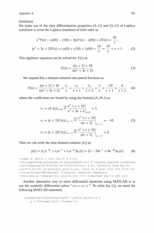
Appendix A 395
(Solution)We make use of the time differentiation properties (A.11) and (A.12) of Laplacetransform to write the Laplace transform of both sides as
s2Y (s) − sy(0) − y′(0) + 3(sY (s) − y(0)) + 2Y (s) = 10
s;
(s2 + 3s + 2)Y (s) = sy(0) + y′(0) + 3y(0) + 10
s= 10
s+ s + 1 (2)
This algebraic equation can be solved for Y (s) as
Y (s) = s(s + 1) + 10
s(s2 + 3s + 2)(3)
We expand this s-domain solution into partial fractions as
Y (s) = s(s + 1) + 10
s(s2 + 3s + 2)= r1
s+ r2
s + 1+ r3
s + 2= 5
s+ −10
s + 1+ 6
s + 2(4)
where the coefficients are found by using the formula (A.28.1) as
r1 = sY (s) |s=0(3)= s2 + s + 10
s2 + 3s + 2
∣∣∣∣s=0
= 5
r2 = (s + 1)Y (s) |s=−1(3)= s2 + s + 10
s(s + 2)
∣∣∣∣s=−1
= −10
r3 = (s + 2)Y (s) |s=−2(3)= s2 + s + 10
s(s + 1)
∣∣∣∣s=−2
= 6
(5)
Thus we can write the time-domain solution y(t) as
y(t) = (r1e−0t + r2e−t + r3e−2t )us(t) = (5 − 10e−t + 6e−2t )us(t) (6)
>>syms s, Ns=[1 1 10]; Ds=[1 3 2 0];>>y=ilaplace(poly2sym(Ns,s)/poly2sym(Ds,s)) % Inverse Laplace transform>>y1=ilaplace((sˆ2+s+10)/(sˆ3+3*sˆ2+2*s)) % Or, directly from Eq.(3)>>t=0:0.01:10; yt=eval(y); plot(t,yt), hold on % plot y(t) for t=[0,10]>>[r,p,k]=residue(Ns,Ds), % Partial fraction expansion>>yt1=real(r.’*exp(p*t)); plot(t,yt1,’r’) % Another way to get y(t)
Another alternative way to solve differential equations using MATLAB is touse the symbolic differential solver “dsolve()”. To solve Eq. (1), we need thefollowing MATLAB statement:
>>y=dsolve(’D2y+3*Dy+2*y=0’,’y(0)=1,Dy(0)=-2’)y = 5+6*exp(-2*t)-10*exp(-t)

396 Appendix A
Table A.2 Properties of Laplace transform
(0) Definition X (s) =L{x(t)} = ∫ ∞0 x(t)e−st dt ; x(t)
L↔ X (s)(1) Linearity αx(t) + βy(t) ↔ αX (s) + βY (s)(2) Time shifting (Real translation) x(t − t1)us (t − t1), t1 > 0 ↔
e−st1{
X (s) + ∫ 0−t1
x(τ )e−sτ dτ}
= e−st1 X (s)
for x(t) = 0 ∀t < 0(3) Frequency shifting (Complex translation) es1 t x(t) ↔ X (s − s1)(4) Real convolution g(t) ∗ x(t) ↔ G(s)X (s)(5) Time derivative (Differentiation property) x ′(t) = d
dt x(t) ↔ s X (s) − x(0)(6) Time integral (Integration property)
∫ t−∞ x(τ )dτ ↔ 1
s X (s) + 1s
∫ 0−∞ x(τ )dτ
(7) Complex derivative t x(t) ↔ − dds X (s)
(8) Complex convolution x(t)y(t) ↔ 12π j
∫ σ0+∞σ0−∞ X (v)Y (s − v)dv
(9) Initial value theorem x(0) = lims→∞ s X (s)
(10) Final value theorem x(∞) = lims→0
s X (s)
Theorem A.1 Stability Condition of an LTI system on its Pole LocationA linear time-invariant (LTI) system having the system or transfer function G(s)/G[z]is stable iff (if and only if) all the poles of G(s)/G[z] are strictly within the left-halfs-plane/the unit circle in the z-plane (see Remarks 2.5, 3.2, and 4.5).
Proof Noting that the system or transfer function of a continuous-time/discrete-timesystem is the Laplace/ z-transform of its impulse response g(t)/g[n], let the systemfunction of a causal LTI (linear time-invariant) system be
G(s) = L{g(t)} =∫ ∞
0g(t)e−st dt
(1a)
G[z] = Z{g[n]} =∑∞
n=0g[n]z−n
(1b)
Taking the absolute value yields
|G(s)| =∣∣∣∣∫ ∞
0g(t)e−st dt
∣∣∣∣≤∫ ∞
0|g(t)||e−st |dt (2a)
|G[z]| =∣∣∣∑∞
n=0g[n]z−n
∣∣∣≤∑∞
n=0|g[n]||z−n| (2b)
Suppose that
G(s) has a pole at s = sp = σp + jωp
with σp > 0 on the RHP (right-halfs-plane)
G[z] has a pole at z = z p = rpe jΩp
with rp > 1 outside the unit circle in thez-plane

Appendix A 397
so that
|G(sp)| = ∞ (3a) |G[z p]| = ∞ (3b)
We can substitute this pole into Eq. (2a)/(2b) to get
∞ (3a)= |G(sp)| (2a)≤∫ ∞
0|g(t)||e−σp t ||e− jωp t |dt ;
∞ ≤∫ ∞
0|g(t)|dt (4a)
∞ (3b)= |G[z p]| (2b)≤∑∞
n=0|g[n]||r−n
p ||e− jΩp n |;∞ ≤
∑∞n=0
|g[n]| (4b)
which contradicts the stability condition (1.2.27a)/(1.2.27b). This implies that ifeven a single pole of a system exists in the unstable region, i.e., on the RHP in thes-plane or outside the unit circle in the z-plane, then the system is unstable. Thiscompletes the proof of the theorem.
The stability condition can be understood more clearly if we expand the systemfunction into the partial fractions and take its inverse transform to write the impuseresponse as
G(s) =∑K
k=0
Ak
s − sk;
g(t) =∑k
k=0akesk t (5a)
G[z] =∑k
k=0
Ak
z − zk;
g[n] =∑K
k=0Ak zn
k (5b)
This shows that even a single pole with Re{sk} > 0 or |zk | > 1 causes the impulseresponse to diverge, which violates the BIBO stability condition (1.2.27).

Appendix BTables of Various Transforms
Table B.1 Definition and properties of the CTFS (continuous-time Fourier series)
(0) Definition Synthesis: xP (t)(2.1.5a)= 1
P
∑∞k=−∞ Xk e jkω0 t , P: period of xP (t)
Analysis: Xk(2.1.5b)= ∫
P xP (t)e− jkω0 t dt, ω0 = 2πP
(1) Linearty axP (t) + byP (t)F↔ a Xk + bYk
(2) Time reversal xP (−t)F↔ X−k
(3) Symmetry for real-valuedfunctions
Real-valued xP (t) = xP,e(t) + xP,o(t)F↔ Xk = X∗
−k
Real-valued and even xP,e(t)F↔ Xk,e = Re{Xk}
Real-valued and odd xP,o(t)F↔ Xk,o = jIm{Xk}
(4) Conjugate x∗P (t)
CTFS↔ X∗−k
(5) Time shifting (Real translation) xP (t − t1) ↔ Xk e− jkω0 t1 = |Xk |∠(φk − kω0t1)
(6) Frequency shifting (Complextranslation)
xP (t)e j Mω0 t CTFS↔ Xk−M
(7) Real convolution(periodic/circular)
xP (t)∗yP (t) = ∫P x(τ )y(t − τ )dτ
CTFS↔ Xk Yk
(8) Complex convolution xP (t)yP (t)CTFS↔ 1
P
∑∞m=−∞ Xm Yk−m
(9) Time differentiation dx(t)dt
CTFS↔ jkω0 Xk
(10) Time integration∫ t−∞ x(τ )dτ
(finite-valued and periodiconly if X0 = 0
)CTFS↔ 1
jkω0Xk
(11) Scalingx(at), a > 0
(periodic with period P/a)CTFS↔ Xk
(with fundamental frequency aω0)
(12) Parseval’s relation∫ ∞−∞ |xP (t)|2dt = 1
P
∑∞k=−∞ |Xk |2
399

400 Appendix B
Table B.2 Definition and properties of the CTFT (continuous-time Fourier transform)
(0) Definition X ( jω) = F{x(t)} (2.2.1a)= ∫∞−∞ x(t)e− jωt dt
(1) Linearity ax(t) + by(t)F↔ aX (ω) + bY (ω)
(2) Time reversal x(−t)F↔
(2.5.2)X (−ω)
(3) Symmetry for real-valued functions Real-valued x(t) = xe(t) + xo(t)F↔ X (ω) = X∗(−ω)
Real-valued and even xe(t)F↔
(2.5.5a)Xe(ω) = Re{X (ω)}
Real-valued and odd xo(t)F↔
(2.5.5a)Xo(ω) = j Im{X (ω)}
(4) Conjugate x∗(t)F↔ X∗(−ω)
(5) Time shifting (Real translation) x(t − t1)F↔
(2.5.6)X (ω)e− jωt1 = X (ω)∠ − t1ω
(6) Frequency shifting (Complextranslation)
x(t)e jω1 t F↔(2.5.7)
X (ω − ω1)
(7) Duality g(t)F↔ f (ω) ⇔
(2.5.9)f (t)
F↔ 2πg(−ω)
(8) Real convolution y(t) = x(t) ∗ g(t)F↔
(2.5.11)Y (ω) = X (ω)G(ω)
(9) Complex convolution y(t) = x(t)m(t)F↔
(2.5.14)Y (ω) = 1
2πX (ω) ∗ M(ω)
(10) Time differentiation dx(t)dt
F↔(2.5.17)
jωX (ω)
(11) Time integration∫ t−∞ x(τ )dτ
F↔(2.5.18)
π X (0)δ(ω) + 1jω X (ω)
(12) Scaling x(at)F↔
(2.5.21)
1|a| X
(ωa
)(13) Time multiplication-Frequency
differentiationt x(t)
F↔(2.5.20)
j d X (ω)dω
(14) Parseval’s relation∫∞−∞ |x(t)|2dt =
(2.5.22)
12π
∫ ∞−∞ |X (ω)|2dω

Appendix B 401
Tabl
eB
.3C
TFS
/CT
FTfo
rba
sic
func
tions
func
tion
x(t)
CT
FSX
k(f
orpe
riod
icfu
nctio
n)C
TFT
X(ω
)(f
orpe
riod
ic/a
peri
odic
func
tion)
(1)
1 P
∞ ∑k=
−∞X
ke
jkω
0t ,
ω0
=2π P
Xk
(2.3
3) →2π P
∞ ∑k=
−∞X
kδ(ω
−kω
0)
(2)
ejω
0t ,
ω0
=2π P
Xk
={ P
for
k=
10
else
whe
re2π
δ(ω
−ω
0)
(3)
cosω
0t,
ω0
=2π P
Xk
={ P
/2
for
k=
±1,··
·0
else
whe
re(E
2.11
.2)
→π
(δ(ω
+ω
0)+
δ(ω
−ω
0))
(4)
sinω
0t,
ω0
=2π P
Xk
=⎧ ⎨ ⎩−
jP/2
for
k=
1jP
/2
fork
=−1
0el
sew
here
(E2.
11.1
)→
jπ(δ
(ω+
ω0)−
δ(ω
−ω
0))
(5)
Con
stan
tfun
ctio
nx(
t)=
1X
k={ P
for
k=
00
else
whe
re(E
2.7.
1)→
2πδ(ω
)
(6)
Impu
lse
trai
n∞ ∑
i=−∞
δ(t
−iP
)X
k=
1∀k
2π P
∞ ∑k=
−∞δ(ω
−kω
0),
ω0
=2π P
(7)
Rec
tang
ular
wav
e∞ ∑
i=−∞
r D(t
−iP
),D
≤P
Xk
=D
sinc
( kω0
D2π
) ,ω
0=
2π P2π P
∞ ∑k=
−∞X
kδ(ω
−kω
0)
(8)
Rec
tang
ular
puls
er D
(t)=
us(
t+
D 2)−
us(
t−
D 2)
N/A
for
anap
erio
dic
func
tion
Dsi
nc(
D 2πω
)(E2.
3.2)
=si
n(D
ω/2)
ω/2
(9)
sin(
Bt)
πt
=B π
sinc
( Bt
π
)N
/Afo
ran
aper
iodi
cfu
nctio
n(E
2.9.
1)→
{ 1fo
r|ω
|≤B
0el
sew
here
(10)
δ(t
)N
/Afo
ran
aper
iodi
cfu
nctio
n1
(11)
us(
t)N
/Afo
ran
aper
iodi
cfu
nctio
n(E
2.8.
6)→
1 jω+
πδ(ω
)
(12)
e−at u
s(t)
,R
e{a}>
0N
/Afo
ran
aper
iodi
cfu
nctio
n1
a+jω
(13)
te−a
t us(
t),R
e{a}>
0N
/Afo
ran
aper
iodi
cfu
nctio
n1
(a+
jω)2
(14)
tM−1
(M−1
)!e−a
t us(
t),R
e{a}>
0N
/Afo
ran
aper
iodi
cfu
nctio
n1
(a+
jω)M

402 Appendix B
Table B.4 Definition and properties of the DTFT (discrete-time Fourier transform)
(0) Definition DTFT: X (Ω) = X [e jΩ] = F{x[n]} (3.1.1)= ∑∞n=−∞ x[n]e− jΩn
IDTFT: x[n] = F−1{X (Ω)} (3.1.3)= 12π
∫2π
X (Ω)e jΩndΩ
(1) Periodicity X (Ω) = X [e jΩ] = X (Ω + 2mπ ) for any integer m
(2) Linearity ax[n] + by[n]F↔ aX (Ω) + bY (Ω)
(3) Time reversal x[−n]F↔
(3.2.3)X (−Ω)
(4) Symmetry for real-valuedsequences
Real-valued x[n] = xe[n] + xo[n]F↔ X (Ω) = X∗(−Ω)
Real-valued and even xe[n]F↔
(3.2.5a)Xe(Ω) = Re{X (Ω)}
Real-valued and odd xo[n]F↔
(3.2.5b)Xo(Ω) = j Im{X (Ω)}
(5) Conjugate x∗[n]F↔ X∗(−Ω)
(6) Time shifting (Realtranslation)
x[n − n1]F↔ X (Ω)e− jΩn1 = X (Ω)∠ − n1Ω
(7) Frequency shifting (Complextranslation)
x[n]e jΩ1n F↔ X (Ω − Ω1)
(8) Real convolution x[n] ∗ g[n]F↔ X (Ω)G(Ω)
(9) Complex convolution(circular)
x[n]m[n]F↔ 1
2πX (Ω) ∗ M(Ω)
(10) Differencing in time x[n] − x[n − 1]F↔(1 − e− jΩ)X (Ω)
(11) Summation in timen∑
m=−∞x[m] = x[n] ∗ us [n]
F↔1
1−e− jΩ X (Ω) + π X (0)∞∑
i=−∞δ(Ω − 2π i)
(12) Scaling x(K )[n] ={
x[n/K ] = x[r ] for n = r K0 elsewhere
F↔(3.2.14)
X (KΩ)
(13) Time multiplication-Frequency differentiation
nx[n]F↔ j d X (Ω)
dΩ
(14) Parseval’s relation∑∞
n=−∞ |x[n]|2 = 12π
∫2π
|X (Ω)|2dΩ

Appendix B 403
Tabl
eB
.5D
efini
tion
and
prop
ertie
sof
the
DFT
/DFS
(dis
cret
e-tim
eFo
urie
rse
ries
)
(0)
Defi
nitio
nX
(k)=
DFT
N{x
[n]}(3
.4.2
)=
∑ N−1
n=0
x[n]
e−j2
πkn
/N
=∑ N
−1n=
0x[
n]W
kn N
x[n]
=ID
FTN{X
(k)}(3
.4.3
)=
1 N
∑ N−1
k=0
X(k
)ej2
πkn
/N
=1 N
∑ N−1
k=0
X(k
)W−k
nN
(1)
Peri
odic
ityX
(k)=
X(k
+m
N)
for
any
inte
ger
m
(2)
Lin
eari
tya
x[n]
+by
[n]D
FT ↔a
X(k
)+bY
(k)
(3)
Tim
ere
vers
alx[
−n]r
N[n
]DFT ↔
XN
(−k)
r N[k
](r
N[k
]=
us[
k]−
us[
k−
N])
whe
rex N
[n]
isth
epe
riod
icre
petit
ion
ofx[
n]w
ithpe
riod
N
(4)
Sym
met
ryfo
rre
al-v
alue
dse
quen
ces
Rea
l-va
lued
x[n]
=x e
[n]+
x o[n
]DFT ↔
X(k
)=
X∗ N
(−k)
r N[k
]
Rea
l-va
lued
and
even
x e[n
]DFT ↔
Xe(
k)=
Re{
X(k
)}R
eal-
valu
edan
dod
dx o
[n]D
FT ↔X
o(k
)=
jIm
{X(k
)}(5
)C
onju
gate
x∗ [n]
DFT ↔
X∗ N
(−k)
r N[k
]
(6)
Dua
lity
g[n]
DFT ↔
f(k)
⇔f[
n]D
FT ↔N
g N(−
k)r N
[k]
(7)
Tim
esh
iftin
g(c
ircu
lar)
x N[n
−M
]rN
[n](
one
peri
odof
circ
ular
shif
t)D
FT ↔W
Mk
NX
(k)
(8)
Freq
uenc
ysh
iftin
g(c
ircu
lar)
(Com
plex
tran
slat
ion)
WN
−Lnx[
n]D
FT ↔X
N(k
−L
)rN
[k](
one
peri
odof
circ
ular
shif
t)
(9)
Rea
lcon
volu
tion
( ∑N
−1i=
0x(
i)y(
n−
i)) r N
[n]D
FT ↔X
(k)Y
(k)
(10)
Com
plex
(cir
cula
r)co
nvol
utio
nx[
n]y[
n]D
FT ↔1 2π
( ∑N
−1i=
0X
N(i
)YN
(k−
i)) r N
[k]
(11)
Scal
ing
x (K
)[n]
={ x[
n/K
]fo
rn
=r
K0
else
whe
reD
FT ↔X
N(K
k)r N
[k]
(12)
Pars
eval
’sre
latio
n∑ n=
<N
>|x[
n]|2
=1 N
∑ k=<
N>
|X(k
)|2w
here
<N
>=
{0,1,
···,
N−
1}

404 Appendix B
Tabl
eB
.6D
FS/D
FTan
dD
TFT
for
basi
cse
quen
ces
Sequ
ence
x[n]
DFS
X(k
)/D
FTX
(k)
(for
peri
odic
/ape
riod
ican
dfin
ite-d
urat
ion
sequ
ence
s)D
TFT
X(Ω
)
(1)
1 P
∑k=
<N
>
Xke
j2π
kn/
P,
P=
NT
X(k
)=
1 TX
k2π P
∞ ∑k=
−∞X
kδ(Ω
−k
2π N)
(2)
ejK
Ω0n,
Ω0
=2π N
X(k
)={ N
for
k=
K,
K±
N,
K±
2N
,··
·0
else
whe
re(3
.1.5
)→
2π∞ ∑
k=−∞
δ(Ω
−K
Ω0−
2πk)
(3)
cos
KΩ
0n,
Ω0
=2π N
X(k
)={ N
/2
for
k=
±K,±K
±N
,··
·0
else
whe
re(E
3.7.
2)→
π∞ ∑
k=−∞
δ(Ω
+K
Ω0−
2πk)
+δ(Ω
−K
Ω0−
2πk)
(4)
sin
KΩ
0n,
Ω0
=2π N
X(k
)=⎧ ⎨ ⎩−
jN/2
for
k=
K,
K±
N,··
·jN
/2
for
k=
−K,−K
±N
,··
·0
else
whe
re
(E3.
7.1)
→jπ
∞ ∑k=
−∞δ(Ω
+K
Ω0−
2πk)
−δ(Ω
−K
Ω0−
2πk)
(5)
Con
stan
tseq
uenc
ex[
n]=
1X
(k)={ N
for
k=
0,±N
,±2
N,··
·0
else
whe
re(E
3.6.
1)→
2π∞ ∑
k=−∞
δ(Ω
−2π
k)
(6)
∞ ∑i=
−∞δ[n
−iN
]X
(k)=
1∀k
2π N
∞ ∑k=
−∞δ(Ω
−kΩ
0),
Ω0
=2π N
(7)
Rec
tang
ular
wav
e∞ ∑
i=−∞
r 2M
+1[n
−iM
],2
M+
1≤
N
X(k
)=
sin(
kΩ0(2
M+
1)/2)
sin(
kΩ0/2)
,Ω
0=
2π N2π N
∞ ∑k=
−∞X
(k)δ
(Ω−
kΩ0)
(8)
Rec
tang
ular
puls
er 2
M+1
[n]
=u
s[n
+M
]−u
s[n
−M
−1]
X(k
)=
sin(
kΩ0(2
M+
1)/2)
sin(
kΩ0/2)
with
Ω0
=2π N
(E3.
1.2)
→si
n(Ω
(2M
+1)
/2)
sin(
Ω/2)

Appendix B 405
Tabl
eB
.6(c
ontin
ued)
Sequ
ence
x[n]
DFS
X(k
)/D
FTX
(k)
(for
peri
odic
/ape
riod
ican
dfin
ite-d
urat
ion
sequ
ence
s)D
TFT
X(Ω
)
(9)
sin(
Bn)
πn
=B π
sinc
( Bn
π
)N
/Afo
ran
infin
ite-d
urat
ion
aper
iodi
cse
quen
ce(E
3.5.
1)→
{ 1fo
r|Ω
−2m
π|≤
B≤
π
0el
sew
here
(10)
δ[n
]X
(k)=
1∀0
≤k
≤N
−1
(E3.
4.1)
→1
(11)
us[
n]N
/Afo
ran
infin
ite-d
urat
ion
aper
iodi
cse
quen
ce(E
3.8.
6)→
1
1−
e−jΩ
n+
π∞ ∑
i=−∞
δ(Ω
−2π
i)
(12)
anu
s[n]
with
|a|<
1N
/Afo
ran
infin
ite-d
urat
ion
aper
iodi
cse
quen
ce(E
3.2.
1)→
1
1−
ae−
jΩ
(13)
(n+
1)an
us[
n],
|a|<
1N
/Afo
ran
infin
ite-d
urat
ion
aper
iodi
cse
quen
ce1
(1−
ae−
jΩ)2
(14)
a|n|w
ith|a|
<1
N/A
for
anin
finite
-dur
atio
nap
erio
dic
sequ
ence
(E3.
3.1)
→1
−a2
1−
2aco
sΩ+
a2

406 Appendix B
Table B.7 Definitions and properties of the Laplace transform and z-transform

Appendix B 407Ta
ble
B.8
Lap
lace
tran
sfor
ms
and
z-tr
ansf
orm
sof
basi
cfu
nctio
ns/s
eque
nces
X(s
)=
L{x(
t)}
x(t)
x[n]
X[z
]=
Z{x
[n]}
1δ(t
)(1
)1 T
δ[n
]1 T
e−t1s
δ(t
−t 1
)(2
)1 T
δ[n
−n 1
]1 T
z−n1
1 su
s(t)
(3)
us[
n]z
z−
1=
1
1−
z−1
1 s2t
us(
t)(4
)n
Tu
s[n]
Tz
(z−
1)2
M!
sM+1
tMu
s(t)
(5)
(nT
)Mu
s[n]
lim a→0(−
1)M
∂M
∂a
M
(z
z−
e−a
T
)
1
s+
ae−a
t us(
t)(6
)e−a
Tn
us[
n]=
bnu
s[n]
z
z−
e−a
T=
z
z−
b(b
=e−a
T)
1
(s+
a)2
te−a
tu
s(t)
(7)
nT
e−aT
nu
s[n]
Tze
−aT
(z−
e−a
T)2
M!
(s+
a)M
+1tM
e−at
us(
t)(8
)(n
T)M
e−aT
nu
s[n]
(−1)
M∂
M
∂a
M
(z
z−
e−a
T
)
ω
s2+
ω2
sin
ωt
us(
t)(9
)si
n(ω
Tn)
us[
n]z
sin
ωT
z2−
2zco
sωT
+1
ω
(s+
σ)2
+ω
2e−σ
tsi
nω
tu
s(t)
(10)
e−σT
nsi
n(ω
Tn)
us[
n]ze
−σT
sin
ωT
(z−
e−σ
Tco
sωT
)2+
e−2σ
Tsi
n2ω
T
s
s2+
ω2
cosω
tu
s(t)
(11)
cos(
ωT
n)u
s[n]
z(z−
cosω
T)
z2−
2zco
sωT
+1
s+
σ
(s+
σ)2
+ω
2e−σ
tco
sωt
us(
t)(1
2)e−σ
Tn
cos(
ωT
n)u
s[n]
z(z−
e−σT
cosω
T)
(z−
e−σ
Tco
sωT
)2+
e−2σ
Tsi
n2ω
T

408 Appendix B
Table B.9 Bilateral z-transform of basic sequences
x[n] X[z] = Z{x[n]} = ∑∞n=−∞ x[n]z−n with ROC
(1) δ[n] 1 All z
(2) δ[n − n1] z−n1 All z except 0 (for m > 0) or ∞(for m < 0)
(3) us [n] zz−1 = 1
1−z−1 |z| > 1
(4) −us [−n − 1] zz−1 = 1
1−z−1 |z| < 1
(5) e−σ T nus [n] = anus [n] zz−a = 1
1−az−1 (a = e−σ T ) |z| > |a|(6) −bnus [−n − 1] z
z−b = 11−bz−1 |z| < |b|
(7) e−σ T |n| = a|n| zz−a − z
z−1/a (a = e−σ T ) |a| < |z| <∣∣ 1
a
∣∣(8) nus [n] z
(z−1)2 |z| > 1
(9) −nus [−n − 1] z(z−1)2 |z| < 1
(10) nanus [n] az(z−a)2 |z| > |a|
(11) −nbnus [−n − 1] bz(z−b)2 |z| < |b|
(12) n2 an us [n] az(z+a)(z−a)3 |z| > |a|
(13) −n2bnus [−n − 1] bz(z+b)(z−b)3 |z| < |b|
(14) n(n−1)···(n−K+2)(K−1)! an−(K−1)us [n] z
(z−a)K |z| > |a|(15) sin(Ω1n)us [n] z sin Ω1
(z−cos Ω1)2+sin2 Ω1= z sin Ω1
z2−2z cos Ω1+1 |z| > 1
(16) cos(Ω1n)us [n] z(z−cos Ω1)(z−cos Ω1)2+sin2 Ω1
= z(z−cos Ω1)z2−2z cos Ω1+1 |z| > 1
(17) rn sin(Ω1n)us [n] zr sin Ω1
(z−r cos Ω1)2+r2 sin2 Ω1= zr sin Ω1
z2−2zr cos Ω1+r2 |z| > |r |(18) rn cos(Ω1n)us [n] z(z−r cos Ω1)
(z−r cos Ω1)2+r2 sin2 Ω1= z(z−r cos Ω1)
z2−2zr cos Ω1+r2 |z| > |r |

Appendix COperations on Complex Numbers, Vectors,and Matrices
C.1 Complex Addition
(a1 + jb1) + (a2 + jb2) = (a1 + a2) + j(b1 + b2) (C.1)
C.2 Complex Multiplication
Rectangular form: (a1 + jb1) × (a2 + jb2) = (a1a2 − b1b2) + j(a1b2 + b1a2)
(C.2a)
Polar form: r1∠θ1 × r2∠θ2 = r1e jθ1r2e jθ2 = r1r2e j(θ1+θ2) = r1r2∠(θ1 + θ2)(C.2b)
C.3 Complex Division
Rectangular form:a2 + jb2
a1 + jb1= a2 + jb2
a1 + jb1× a1 − jb1
a1 − jb1
= a1a2 + b1b2
a21 + b2
1
+ ja1b2 − a2b1
a21 + b2
1
(C.3a)
Polar form:r2∠θ2
r1∠θ1= r2e jθ2
r1e jθ1= r2
r1e j(θ2−θ1) = r2
r1∠(θ2 − θ1) (C.3b)
C.4 Conversion Between Rectangular Formand Polar/Exponential Form
ar + jai = r∠θ = re jθ with r = |ar + jai | =√
a2r + a2
i and θ = tan−1 ai
ar(C.4)
409
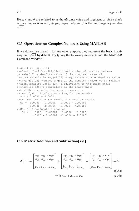
410 Appendix C
Here, r and θ are referred to as the absolute value and argument or phase angleof the complex number ar + jai , respectively and j is the unit imaginary number√−1.
C.5 Operations on Complex Numbers Using MATLAB
If we do not use i and j for any other purpose, they represent the basic imagi-nary unit
√−1 by default. Try typing the following statements into the MATLABCommand Window:
>>c1= 1+2i; c2= 3-4i;>>c1*c2, c1/c2 % multiplication/division of complex numbers>>r=abs(c2) % absolute value of the complex number c2>>sqrt(real(c2)ˆ2+imag(c2)ˆ2) % equivalent to the absolute value>>th=angle(c2) % phase angle of the complex number c2 in radians>>atan2(imag(c2),real(c2)) % equivalent to the phase angle>>imag(log(c2)) % equivalent to the phase angle>>th*180/pi % radian-to-degree conversion>>r*exp(j*th) % polar-to-rectangular conversionans = 3.0000 - 4.0000i
>>C= [1+i 1-2i; -1+3i -1-4i] % a complex matrixC1 = 1.0000 + 1.0000i 1.0000 - 2.0000i
-1.0000 + 3.0000i -1.0000 - 4.0000i>>C1= C’ % conjugate transpose
C1 = 1.0000 - 1.0000i -1.0000 - 3.0000i1.0000 + 2.0000i -1.0000 + 4.0000i
C.6 Matrix Addition and Subtraction[Y-1]
A + B =
⎡⎢⎢⎣
a11 a12 · a1N
a21 a22 · a2N
· · · ·aM1 aM2 · aM N
⎤⎥⎥⎦ +
⎡⎢⎢⎣
b11 b12 · b1N
b21 b22 · b2N
· · · ·bM1 bM2 · bM N
⎤⎥⎥⎦ =
⎡⎢⎢⎣
c11 c12 · c1N
c21 c22 · c2N
· · · ·cM1 cM2 · cM N
⎤⎥⎥⎦ = C
(C.5a)
with amn + bmn = cmn (C.5b)
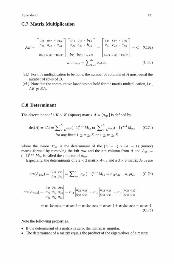
Appendix C 411
C.7 Matrix Multiplication
AB =
⎡⎢⎢⎣
a11 a12 · a1K
a21 a22 · a2K
· · · ·aM1 aM2 · aM K
⎤⎥⎥⎦⎡⎢⎢⎣
b11 b12 · b1N
b21 b22 · b2N
· · · ·bK 1 bK 2 · bK N
⎤⎥⎥⎦ =
⎡⎢⎢⎣
c11 c12 · c1N
c21 c22 · c2N
· · · ·cM1 cM2 · cM N
⎤⎥⎥⎦ = C (C.6a)
with cmn =∑K
k=1amkbkn (C.6b)
(cf.) For this multiplication to be done, the number of columns of A must equal thenumber of rows of B.
(cf.) Note that the commutative law does not hold for the matrix multiplication, i.e.,AB �= B A.
C.8 Determinant
The determinant of a K × K (square) matrix A = [amn] is defined by
det(A) = |A| =∑K
k=0akn(−1)k+n Mkn or
∑K
k=0amk(−1)m+k Mmk (C.7a)
for any fixed 1 ≤ n ≤ K or 1 ≤ m ≤ K
where the minor Mkn is the determinant of the (K − 1) × (K − 1) (minor)matrix formed by removing the kth row and the nth column from A and Akn =(−1)k+n Mkn is called the cofactor of akn .
Especially, the determinants of a 2 × 2 matrix A2×2 and a 3 × 3 matrix A3×3 are
det(A2×2) =∣∣∣∣a11 a12
a21 a22
∣∣∣∣ =∑2
k=1akn(−1)k+n Mkn = a11a22 − a12a21 (C.7b)
det(A3×3) =∣∣∣∣∣∣a11 a12 a13
a21 a22 a23
a31 a32 a33
∣∣∣∣∣∣ = a11
∣∣∣∣a22 a23
a32 a33
∣∣∣∣ − a12
∣∣∣∣a21 a23
a31 a33
∣∣∣∣ + a13
∣∣∣∣a21 a22
a31 a32
∣∣∣∣= a11(a22a33 − a23a32) − a12(a21a33 − a23a31) + a13(a21a32 − a22a31)
(C.7c)
Note the following properties.
• If the determinant of a matrix is zero, the matrix is singular.• The determinant of a matrix equals the product of the eigenvalues of a matrix.
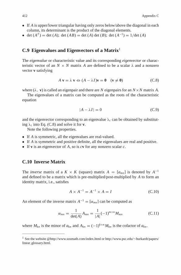
412 Appendix C
• If A is upper/lower triangular having only zeros below/above the diagonal in eachcolumn, its determinant is the product of the diagonal elements.
• det (AT ) = det (A); det (AB) = det (A) det (B); det (A−1) = 1/det (A)
C.9 Eigenvalues and Eigenvectors of a Matrix1
The eigenvalue or characteristic value and its corresponding eigenvector or charac-teristic vector of an N × N matrix A are defined to be a scalar λ and a nonzerovector v satisfying
A v = λ v ⇔ (A − λI )v = 0 (v �= 0) (C.8)
where (λ, v) is called an eigenpair and there are N eigenpairs for an N×N matrix A.The eigenvalues of a matrix can be computed as the roots of the characteristic
equation
|A − λI | = 0 (C.9)
and the eigenvector corresponding to an eigenvalue λi can be obtained by substitut-ing λi into Eq. (C.8) and solve it for v.
Note the following properties.
• If A is symmetric, all the eigenvalues are real-valued.• If A is symmetric and positive definite, all the eigenvalues are real and positive.• If v is an eigenvector of A, so is cv for any nonzero scalar c.
C.10 Inverse Matrix
The inverse matrix of a K × K (square) matrix A = [amn] is denoted by A−1
and defined to be a matrix which is pre-multiplied/post-multiplied by A to form anidentity matrix, i.e., satisfies
A × A−1 = A−1 × A = I (C.10)
An element of the inverse matrix A−1 = [αmn] can be computed as
αmn = 1
det(A)Amn = 1
|A| (−1)m+n Mmn (C.11)
where Mkn is the minor of akn and Akn = (−1)k+n Mkn is the cofactor of akn .
1 See the website @http://www.sosmath.com/index.html or http://www.psc.edu/∼burkardt/papers/linear glossary.html.
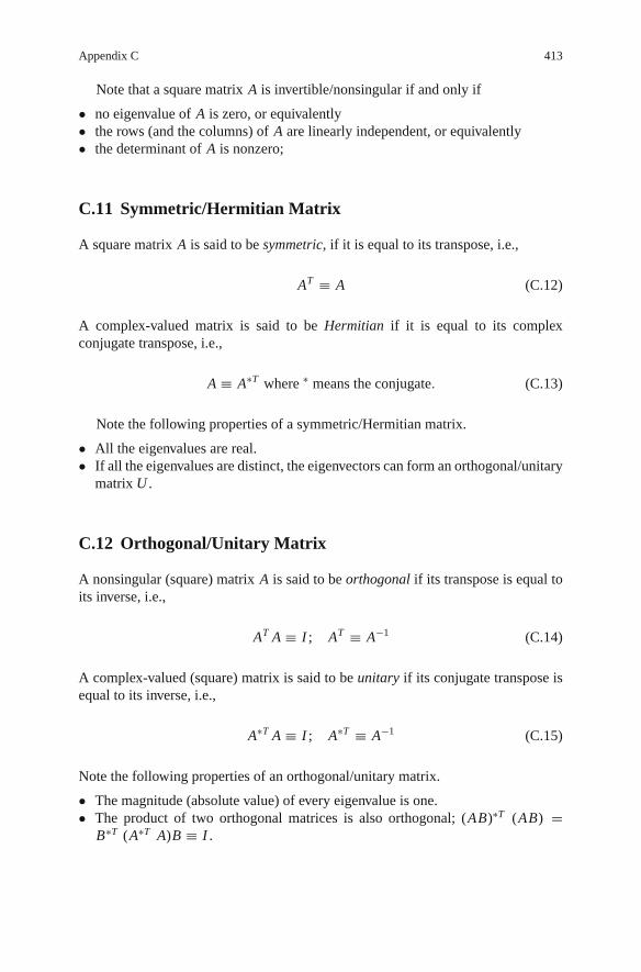
Appendix C 413
Note that a square matrix A is invertible/nonsingular if and only if
• no eigenvalue of A is zero, or equivalently• the rows (and the columns) of A are linearly independent, or equivalently• the determinant of A is nonzero;
C.11 Symmetric/Hermitian Matrix
A square matrix A is said to be symmetric, if it is equal to its transpose, i.e.,
AT ≡ A (C.12)
A complex-valued matrix is said to be Hermitian if it is equal to its complexconjugate transpose, i.e.,
A ≡ A∗T where ∗ means the conjugate. (C.13)
Note the following properties of a symmetric/Hermitian matrix.
• All the eigenvalues are real.• If all the eigenvalues are distinct, the eigenvectors can form an orthogonal/unitary
matrix U .
C.12 Orthogonal/Unitary Matrix
A nonsingular (square) matrix A is said to be orthogonal if its transpose is equal toits inverse, i.e.,
AT A ≡ I ; AT ≡ A−1 (C.14)
A complex-valued (square) matrix is said to be unitary if its conjugate transpose isequal to its inverse, i.e.,
A∗T A ≡ I ; A∗T ≡ A−1 (C.15)
Note the following properties of an orthogonal/unitary matrix.
• The magnitude (absolute value) of every eigenvalue is one.• The product of two orthogonal matrices is also orthogonal; (AB)∗T (AB) =
B∗T (A∗T A)B ≡ I .

414 Appendix C
C.13 Permutation Matrix
A matrix P having only one nonzero element of value 1 in each row and column iscalled a permutation matrix and has the following properties.
• Pre-multiplication/post-multiplication of a matrix A by a permutation matrix P ,i.e., PA or AP yields the row/column change of the matrix A, respectively.
• A permutation matrix A is orthogonal, i.e., AT A ≡ I .
C.14 Rank
The rank of an M × N matrix is the number of linearly independent rows/columnsand if it equals min (M, N ), then the matrix is said to be of maximal or full rank;otherwise, the matrix is said to be rank-deficient or to have rank-deficiency.
C.15 Row Space and Null Space
The row space of an M ×N matrix A, denoted by R (A), is the space spanned by therow vectors, i.e., the set of all possible linear combinations of row vectors of A thatcan be expressed by ATααα with an M-dimensional column vector ααα. On the otherhand, the null space of the matrix A, denoted by N (A), is the space orthogonal(perpendicular) to the row space, i.e., the set of all possible linear combinations ofthe N -dimensional vectors satisfying Ax = 0.
C.16 Row Echelon Form
A matrix is said to be of row echelon form [W-6] if
• each nonzero row having at least one nonzero element has a 1 as its first nonzeroelement, and
• the leading 1 in a row is in a column to the right of the leading 1 in the upper row.• All-zero rows are below the rows that have at least one nonzero element.
A matrix is said to be of reduced row echelon form if it satisfies the above conditionsand additionally, each column containing a leading 1 has no other nonzero elements.
Any matrix, singular or rectangular, can be transformed into this form throughthe Gaussian elimination procedure, i.e., a series of elementary row operations,or equivalently, by using the MATLAB built-in routine “rref()”. For example,we have
A =⎡⎣ 0 0 1 3
2 4 0 −81 2 1 −1
⎤⎦ row→
change
⎡⎣ 2 4 0 −8
0 0 1 31 2 1 −1
⎤⎦
rowdivision
→row
subtraction
⎡⎣ 1 2 0 −4
0 0 1 30 0 1 3
⎤⎦ row→
subtraction
⎡⎣ 1 2 0 −4
0 0 1 30 0 0 0
⎤⎦ = rre f (A)

Appendix C 415
Once this form is obtained, it is easy to compute the rank, the determinant, and theinverse of the matrix, if only the matrix is invertible.
C.17 Positive Definiteness
A square matrix A is said to be positive definite if
x∗T A x > 0 for any nonzero vector x (C.16)
A square matrix A is said to be positive semi-definite if
x∗T A x ≥ 0 for any nonzero vector x (C.17)
Note the following properties of a positive definite matrix A.
• A is nonsingular and all of its eigenvalues are positive, and• the inverse of A is also positive definite.
There are similar definitions for negative definiteness and negative semi-definiteness.Note the following property, which can be used to determine if a matrix is
positive (semi-) definite or not. A square matrix is positive definite if and only if
(i) every diagonal element is positive and(ii) every leading principal minor matrix has positive determinant.
On the other hand, a square matrix is positive semi-definite if and only if
(i) every diagonal element is nonnegative and(ii) every principal minor matrix has nonnegative determinant.
Note also that the principal minor matrices are the sub-matrices taking the diagonalelements from the diagonal of the matrix A and, say for a 3×3 matrix, the principalminor matrices are
a11, a22, a33,
[a11 a12
a21 a22
],
[a22 a23
a32 a33
],
[a11 a13
a31 a33
],
⎡⎣a11 a12 a13
a21 a22 a23
a31 a32 a33
⎤⎦
among which the leading ones are
a11,
[a11 a12
a21 a22
],
⎡⎣a11 a12 a13
a21 a22 a23
a31 a32 a33
⎤⎦

416 Appendix C
C.18 Scalar(Dot) Product and Vector(Cross) Product
A scalar product of two N -dimensional vectors x and y is denoted by x · y and isdefined by
x · y =∑N
n=1xn yn = xT y (C.18)
An outer product of two 3-dimensional column vectors x = [x1 x2 x3]T and y =[y1 y2 y3]T is denoted by x × y and is defined by
x × y =
⎡⎣ x2 y3 − x3 y2
x3 y1 − x1 y3
x1 y2 − x2 y1
⎤⎦ (C.19)
C.19 Matrix Inversion Lemma
[Matrix Inversion Lemma]Let A, C and [C−1 + D A−1 B] be well-defined with non-singularity as well
as compatible dimensions. Then we have
[A + BC D]−1 = A−1 − A−1 B[C−1 + D A−1 B]−1 D A−1 (C.20)
Proof We will show that post-multiplying Eq. (C.20) by [A + BC D] yields anidentity matrix.
[A−1 − A−1 B[C−1 + D A−1 B]−1 D A−1][A + BC D]= I + A−1 BC D − A−1 B[C−1 + D A−1 B]−1 D − A−1 B[C−1 + D A−1 B]−1 D A−1 BC D= I + A−1 BC D − A−1 B[C−1 + D A−1 B]−1C−1C D − A−1 B[C−1 + D A−1 B]−1 D A−1 BC D= I + A−1 BC D − A−1 B[C−1 + D A−1 B]−1[C−1 + D A−1 B]C D= I + A−1 BC D − A−1 BC D ≡ I
C.20 Differentiation w.r.t. a Vector
The 1st derivative of a scalar-valued function f (x) w.r.t. a vector x = [x1 x2]T iscalled the gradient of f (x) and defined as
∇ f (x) = d
dxf (x) =
[∂ f/∂x1
∂ f/∂x2
](C.21)

Appendix C 417
Based on this definition, we can write the following equation.
∂
∂xxT y = ∂
∂xyT x = ∂
∂x(x1 y1 + x2 y2) =
[y1
y2
]= y (C.22)
∂
∂xxT x = ∂
∂x(x2
1 + x22 ) = 2
[x1
x2
]= 2x (C.23)
Also with an M × N matrix A, we have
∂
∂xxT Ay = ∂
∂xyT AT x = Ay (C.24a)
∂
∂xyT Ax = ∂
∂xxT AT y = AT y (C.24b)
where
xT Ay =∑M
m=1
∑N
n=1amn xm yn (C.25)
Especially for a square, symmetric matrix A with M = N , we have
∂
∂xxT Ax = (A + AT )x
if A is symmetric→ 2Ax (C.26)
The 2nd derivative of a scalar function f (x) w.r.t. a vector x = [x1 x2]T is called theHessian of f (x) and is defined as
H (x) = ∇2 f (x) = d2
dx2f (x) =
[∂2 f/∂x2
1 ∂2 f/∂x1∂x2
∂2 f/∂x2∂x1 ∂2 f/∂x22
](C.27)
Based on this definition, we can write the following equation:
d2
dx2xT Ax = A + AT if A is symmetric→ 2A (C.28)
On the other hand, the 1st derivative of a vector-valued function f(x) w.r.t. avector x = [x1 x2]T is called the Jacobian of f (x) and is defined as
J (x) = d
dxf(x) =
[∂ f1/∂x1 ∂ f1/∂x2
∂ f2/∂x1 ∂ f2/∂x2
](C.29)

Appendix DUseful Formulas
419

Appendix EMATLAB
Once you installed MATLAB�, you can click the icon like the oneat the right side to run MATLAB. Then you will see the MATLABCommand Window on your monitor as depicted in Fig. E.1, wherea cursor appears (most likely blinking) to the right of the promptlike “>>” waiting for you to type in commands/statements. If youare running MATLAB of version 6.x or above, the main window hasnot only the command window, but also the workspace and command historyboxes on the left-up/down side of the command window, in which you can seethe contents of MATLAB memory and the commands you have typed into theCommand window up to the present time, respectively (see Fig. E.1). You mightclear the boxes by clicking the corresponding submenu under the “Edit” menuand even remove/restore them by clicking the corresponding submenu under the“Desktop/Desktop Layout” menu.
How do we work with the MATLAB Command Window?
– By clicking “File” on the top menu and then “New”/“Open” in the File pull-downmenu, you can create/edit any file with the MATLAB editor.
Fig. E.1 The MATLAB command window with the workspace and command history boxes
421

422 Appendix E
– By clicking “File” on the top menu and then “Set Path” in the File pull-downmenu, you can make the MATLAB search path list include or exclude the pathscontaining the files you want to or not to be run.
– If you are a beginner in MATLAB, then it may be worthwhile to click “Help”on the top menu, “Demos” in the Help pull-down menu, (double-)click any topicthat you want to learn about, and watch the visual explanation about it.
– By typing any MATLAB commands/statements in the MATLAB Command Win-dow, you can use various powerful mathematic/graphic functions of MATLAB.
– If you have an M-file which contains a series of commands/statements composedfor performing a target procedure, you can type in the file name (without theextension “.m”) to run it.
Note the following:
1) the index of an array in MATLAB starts from 1, not 0, and2) a dot(.) must be put before an operator to make a term-wise (element-by-
element) operation.
Table E.1 Functions and Variables in MATLABfunction Remark function Remark
cos(x) exp(x) exponential functionsin(x) log(x) natural logarithmtan(x) log10(x) common logarithmacos(x) cos−1 (x) abs(x) absolute valueasin(x) sin−1 (x) angle(x) phase of a complex
number[rad]atan(x) −π/2 ≤ tan−1 (x) ≤ π/2 sqrt(x) square rootatan2(y,x) −π ≤ tan−1 (y, x) ≤ π real(x) real partcosh(x) (ex + e−x )/2 imag(x) imaginary partsinh(x) (ex − e−x )/2 conj(x) complex conjugatetanh(x) (ex − e−x )/(ex + e−x ) round(x) the nearest integer (round-off)acosh(x) cosh−1 (x) fix(x) the nearest integer towards 0asinh(x) sinh−1 (x) floor(x) the greatest integer ≤ x
rounding downatanh(x) tanh−1 (x) ceil(x) the smallest integer ≥ x
rounding upmax maximum and its index sign(x) 1(positive)/0/-1(negative)min minimum and its index mod(y,x) remainder of y/xsum sum rem(y,x) remainder of y/xprod product eval(f) evaluate an expressionnorm norm feval(f,a) function evaluationsort sort in the ascending order polyval value of a polynomial functionclock present time poly polynomial with given rootsfind index of element(s) roots roots of polynomialtic start a stopwatch timer toc read the stopwatch timer
(elapsed time from tic)date present date

Appendix E 423
Table E.1 (continued)
function Remark function Remark
reserved variables with special meaningi, j
√−1 pi π
eps machine epsilon (smallestpositive number)
Inf, inf largest number (∞)
realmax,realmin
largest/smallest positivenumber
NaN Not a Number(undetermined)
end the end of for-loop or if, while,case statement or an arrayindex
break exit while/for loop
nargin # of input arguments nargout # of output argumentsvarargin variable input argument list varargout variable output argument list
Table E.2 Graphic line specifications used in the plot() command
Line type Point type (Marker symbol) Color
- solid line .(dot) +(plus) ∗(asterisk) r: red m: magenta: dotted line ∧: Δ >: > ◦(circle) g: green y: yellow– dashed line p: � v: ∇ x: x-mark b: blue c: cyan(sky blue)-. dash-dot d: ♦ <: < s: square(�) k: black
Some of mathematical functions and special reserved constants/variables definedin MATLAB are listed in Table E.1. Table E.2 shows the graphic line specificationsused in the plot() command.
E.1 Convolution and Deconvolution
C=conv(A,B)
– For two sequences A = [a1 a2 · · · aN ] and B = [b1 b2 · · · bM ], this routinecomputes their (linear) convolution C = [c1 c2 · · · cN+M−1] as
cn+1 =∑min(n,M−1)
m=max(0,n−N+1)an−m+1bm+1 (E.1)
– It can be used for multiplying two polynomials whose coefficients are A andB, respectively:
(a1x N−1 + · · · + aN−1x + aN )(b1x M−1 + · · · + bM−1x + bM )
= c1x N+M−2 + · · · + cN+M−2x + cN+M−1
– C=xcorr2(A,B) performs two-dimensional convolution of matrices Aand B.
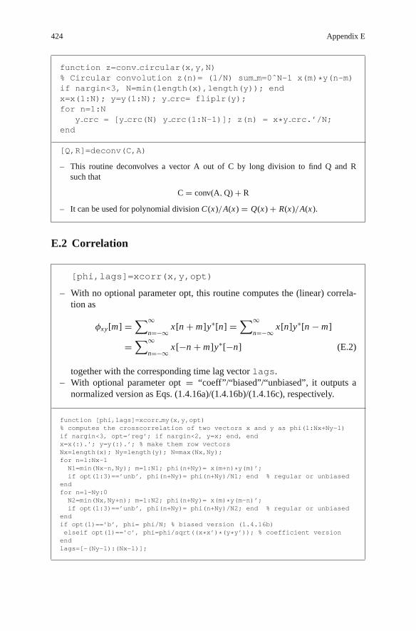
424 Appendix E
function z=conv circular(x,y,N)% Circular convolution z(n)= (1/N) sum m=0ˆN-1 x(m)*y(n-m)if nargin<3, N=min(length(x),length(y)); endx=x(1:N); y=y(1:N); y crc= fliplr(y);for n=1:N
y crc = [y crc(N) y crc(1:N-1)]; z(n) = x*y crc.’/N;end
[Q,R]=deconv(C,A)
– This routine deconvolves a vector A out of C by long division to find Q and Rsuch that
C = conv(A, Q) + R
– It can be used for polynomial division C(x)/A(x) = Q(x) + R(x)/A(x).
E.2 Correlation
[phi,lags]=xcorr(x,y,opt)
– With no optional parameter opt, this routine computes the (linear) correla-tion as
φxy[m] =∑∞
n=−∞ x[n + m]y∗[n] =∑∞
n=−∞ x[n]y∗[n − m]
=∑∞
n=−∞ x[−n + m]y∗[−n] (E.2)
together with the corresponding time lag vector lags.– With optional parameter opt = “coeff”/“biased”/“unbiased”, it outputs a
normalized version as Eqs. (1.4.16a)/(1.4.16b)/(1.4.16c), respectively.
function [phi,lags]=xcorr my(x,y,opt)% computes the crosscorrelation of two vectors x and y as phi(1:Nx+Ny-1)if nargin<3, opt=’reg’; if nargin<2, y=x; end, endx=x(:).’; y=y(:).’; % make them row vectorsNx=length(x); Ny=length(y); N=max(Nx,Ny);for n=1:Nx-1N1=min(Nx-n,Ny); m=1:N1; phi(n+Ny)= x(m+n)*y(m)’;if opt(1:3)==’unb’, phi(n+Ny)= phi(n+Ny)/N1; end % regular or unbiased
endfor n=1-Ny:0N2=min(Nx,Ny+n); m=1:N2; phi(n+Ny)= x(m)*y(m-n)’;if opt(1:3)==’unb’, phi(n+Ny)= phi(n+Ny)/N2; end % regular or unbiased
endif opt(1)==’b’, phi= phi/N; % biased version (1.4.16b)elseif opt(1)==’c’, phi=phi/sqrt((x*x’)*(y*y’)); % coefficient version
endlags=[-(Ny-1):(Nx-1)];

Appendix E 425
function phi=xcorr circular(x,y,N)% Circular (cyclic) correlation of x and y with period Nif nargin<2, y=x; endNx = length(x); Ny = length(y);if nargin<3, N=max(Nx,Ny); endif Nx<N, x = [x zeros(1,N-Nx)]; elseif N<Nx, x = x(1:N); endif Ny<N, y = [y zeros(1,N-Ny)]; elseif N<Ny, y = y(1:N); endfor n=1:N, phi(n) = x*y’/N; y = [y(N) y(1:N-1)]; end
PHI=xcorr2(X,Y)
– Two-dimensional cross-correlation of matrices X and Y
E.3 CTFS (Continuous-Time Fourier Series)
function [c,kk]=CTFS exponential(x,P,N)% Find the complex exponential Fourier coefficients c(k) for k=-N:N% x: A periodic function with period P% P: Period, N: Maximum frequency index to specify the frequency rangew0=2*pi/P; % the fundamental frequency [rad/s]xexp jkw0t = [x ’(t).*exp(-j*k*w0*t)’];xexp jkw0t= inline(xexp jkw0t ,’t’,’k’,’w0’);kk=-N:N; tol=1e-6; % the frequency range tolerance on numerical errorfor k=kk
c(k+N+1)= quadl(xexp jkw0t,-P/2,P/2,tol,[],k,w0); % Eq. (2.1.5b)end
E.4 DTFT (Discrete-Time Fourier Transform)
function [X,ph]=DTFT(x,W,n0)% DTFT of x[n] for frequency W regarding the 1st sample as the n0-th one.Nt =length(x); n=0:Nt-1;if nargin<3, n0 = -floor(Nt/2); endX= x*exp(-j*(n+n0)’*W); % Eq.(3.1.1)if nargout==2, ph=angle(X); X=abs(X); end
E.5 DFS/DFT (Discrete Fourier Series/Transform)
function [X,ph]=DFS(x,N,n0)% N-point DFS/DFT of x[n] regarding the 1st sample as the n0-th one.if nargin<3, n0 = 0; endn=n0+[0:length(x)-1]; k=[0:N-1];X= x*exp(-j*2*pi*n’*k/N); % Eq.(3.4.7)If nargout==2, ph=angle(X); X=abs(X); end

426 Appendix E
E.6 FFT (Fast Fourier Transform)
X=fft(x,N) or fft(x)
– This routine computes the N-point DFT X(k) of a given sequence x[n],where the sequence will be zero-padded or truncated so that its resultinglength will be N. If the 2nd input argument is not given, the DFT size willbe set to the length of the sequence. In case the 1st input argument x is amatrix, X will also be a matrix, each column of which is the FFT of thecorresponding column of x.
– Note that, to exploit the computational efficiency of FFT, the DFT size Nshould be chosen as a power of 2 greater than or equal to the length of thesequence.
x=ifft(X,N) or ifft(X)
– This routine computes the N-point IDFT x[n] of a given sequence X(k),where the sequence will be zero-padded or truncated so that its resultinglength will be N. If the 2nd input argument is not given, the IDFT size willbe set to the length of the sequence. In case the 1st input argument x is amatrix, x will also be a matrix, each column of which is the IDFT of thecorresponding column of X.
– Note that, to exploit the computational efficiency of FFT, the IDFT size Nshould be chosen as a power of 2 greater than or equal to the length of thesequence.
X=fft2(x,M,N) or fft2(x)
– This routine computes the two-dimensional DFT X(k,l) of a given matrixx[m,n], where each column/row of x will be zero-padded or truncated so thatthe resulting matrix size will be M × N. If the 2nd and 3rd input argumentsare not given, the DFT sizes will be set to the row/column size. In fact,“fft2(x,M,N)” is equivalent to “fft(fft(x,M).’),N).′”
x=ifft2(X,M,N) or ifft2(X)
– This routine computes the two-dimensional IDFT x[m,n] of a given matrixX(k,l), where each column/row of X will be zero-padded or truncated so thatthe resulting matrix size will be M × N. If the 2nd and 3rd input argumentsare not given, the IDFT sizes will be set to the row/column size. In fact,“ifft2(x,M,N)” is equivalent to “ifft(ifft(x,M).’),N).′”

Appendix E 427
y=fftshift(x)
– This routine swaps the first and second halves of the input vector x if x isa vector and swaps quadrants one and three with quadrants two and fourif x is a matrix. It is used to rearrange the FFT sequence so that the zero(DC) frequency component is located at the center with the negative/positivefrequency ones on the left/right side.
E.7 Windowing
function xw=windowing(x,w,opt)N= length(x);if isnumeric(w)
xw= x; Nw2=floor((N-w)/2); xw(1:Nw2)=0; xw(Nw2+w+1:end)=0;elseswitch lower(w(1:2))
case {’bt’,’tt’}, w= bartlett(N); % window(bartlett,N)case ’bk’, w= blackman(N); % window(@blackman,N)case ’cb’, if nargin<3, r=100; else r=opt; end
w= chebwin(N,r); % window(@chebwin,N,r)case ’gs’, if nargin<3, alpha=2.5; else alpha=opt; end
w= gausswin(N,alpha); % window(@gausswin,N,alpha)case ’hm’, w= hamming(N); % window(@hamming,N)case ’hn’, w= hanning(N); % window(@hanning,N)case ’ks’, if nargin<3, beta=0.5; else beta=opt; end
w= kaiser(N,beta); % window(@kaiser,N,beta)otherwise w= x;
endif size(x,1)==1, w=w.’; endxw = x.*w;
end
(cf.) You can just type “window” or “wintool” into the MATLAB Command win-dow to open the Window Design & Analysis Tool. Type “doc window/signal”/“doc window” to see other usages of the signal processing toolboxor filter design toolbox function “window”.
E.8 Spectrogram (FFT with Sliding Window)
[X,F,T]=specgram(x,N,Fs,WND,Noverlap) in MATLAB 6.xversions
– This STFT (Short-Time Fourier Transform) routine computes the spectro-gram, i.e., N-point DFT X(k,m) of mth segment that is windowed by WNDand overlaps with neighboring segment by Noverlap (whose default value islength(WND)/2), where the length of WND must be greater than Noverlap,but not greater than N.

428 Appendix E
– Input• WND: Window sequence given as a column vector of length Nw such that
Noverlap < Nw <= N
If a scalar is given as WND, a Hamming window of length N is used.• N: DFT size whose default value is min(256,length(x)).• Fs: Sampling frequency which does not affect the spectrogram but is used
for scaling plots and its default value is 2 Hz.• You can use the default value for any parameter by leaving it off or
using [].
– Output• X: STFT X(k,m) of x with time and frequency increasing linearly across
its columns, from left to right and down its rows, starting at 0, respec-tively. The number of coumns of X will be Nc = fix((length(x)-Noverlap)/(length(WND)-Noverlap)). The number of rows of X willbe Nr = ceil((N + 1)/2) or N depending on whether x is real orcomplex-valued.
• F and T: Nr normalized frequencies (Ω/π) in Hz and Nc times in columnvectors
– With no output arguments, the routine plots the absolute value of the spec-trogram in the current figure, using imagesc(T,F,20∗log10(abs(X))), whereT is created with its starting point shifted by (Nw-Noverlap)/2. Then “axisxy”, and “colormap(jet)” are used so that the low frequency content of thefirst portion of the signal is displayed in the lower left corner of the axes.>>imagesc(T,F,20∗log10(abs(X)+eps)); axis xy; colormap(jet)
(Example) Compute the spectrogram of a quadratic chirp.
Fs=1e3; Ts=1/Fs; t=0:Ts:2; % 0˜2 secs @ 1kHz sample ratex= chirp(t,0,1,150,’q’); % quadratic chirp start @ 0 & cross 150Hz at t=1N=64; Nhw=N; % The DFT size and the length of the Hanning windowNoverlap=32; [X,F,T] = specgram(x,N,Fs,Nhw,Noverlap);specgram(x,N,Fs,Nhw,Noverlap); % Display the spectrogramtitle(’Quadractic Chip: start at 0Hz and cross 150Hz at t=1sec’)
[X,F,T,P]=spectrogram(x,WND,Noverlap,N,Fs) in MATLAB7.x versions
– This STFT routine computes the spectrogram, i.e., N-point DFT X(k,m)of mth segment that is windowed by WND and overlaps with neighboringsegment by Noverlap.
– By default, x is divided into eight segments. If x cannot be divided exactlyinto eight segments, it is truncated. Also by default, the DFT size N is set

Appendix E 429
to the maximum of 256 and the next power of 2 greater than the lengthof each segment of x. WND is a Hamming window of length N. Noverlapis the value producing 50% overlap between segments. Fs is the samplingfrequency, which defaults to normalized frequency 1 Hz.
– Each column of X contains an estimate of the short-term, time-localized fre-quency content of x. Time increases across the columns of S and frequencyincreases down the rows.
– The number of rows of X will be Nr = ceil((N + 1)/2) or N depending onwhether x is real-valued or complex-valued.
– The number of coumns of X will be Nc = fix((length(x)-Noverlap)/(length(WND)-Noverlap)).
– If WND is given as an integer, x is divided into segments of length WND andeach segment is windowed by a Hamming window. If WND is a vector, x isdivided into segments equal to the length of WND and then each segment iswindowed by the window vector WND.
– Noverlap must be an integer smaller than WND (an integer) or its length ifWND is a vector.
– If the 4th input argument is given as not a scalar meaning the DFT size, buta vector of frequency[Hz], spectrogram(x,WND,Noverlap,F) computes thespectrogram at the frequencies in F using the Goertzel algorithm.
– The 2nd output F is the frequency vector of length N and the 3rd output Tthe time vector of length Nc at which the spectrogram is computed, whereeach value of T corresponds to the center of each segment.
– The 4th output P is a matrix of the same size as x containing the PSD ofeach segment. For real x, each column of P has the one-sided periodogramestimate of the PSD of each segment. If x is complex or a frequency vectoris given as the 4th input, P has the two-sided PSD.
E.9 Power Spectrum
[Pxy,F]=cpsd(x,y,WND,Noverlap,Nfft,Fs)
– This routine computes the one/two-sided CPSD (Cross Power Spectral Den-sity) estimate Pxy of two real/complex-valued signal vectors x and y usingWelch’s averaged periodogram method. For real signals, Pxy has length(Nfft/2 + 1) if Nfft is even, and (Nfft + 1)/2 if Nfft is odd. For complexsignals, Pxy always has length Nfft.
– By default, x is divided into 8 sections (with 50% overlap), each of whichis windowed with a Hamming window and eight modified periodograms arecomputed and averaged.

430 Appendix E
– If WND is a vector, the signal vectors are divided into overlapping sectionsof length equal to the length of WND, and then each section is windowedwith WND. If WND is an integer, x and y are divided into sections of lengthWND, and a Hamming window of equal length is used. If the length of x andy is such that it cannot be divided exactly into integer number of sectionsoverlapped by Novelap samples (or 50% by default), they will be truncatedaccordingly. Noverlap must be an integer smaller than WND (given as aninteger) or the length of WND (given as a vector).
– Nfft specifies the DFT size used to calculate the CPSD estimate and itsdefault value is the maximum of 256 or the next power of 2 greater thanthe length of each section of x (and y).
– Note that if Nfft is greater than the segment length, the data is zero-padded.If Nfft is less than the segment, the segment is “wrapped” to make the lengthequal to Nfft. This produces the correct FFT when Nfft < L, L being signalor segment length.
– If the sampling frequency Fs is not given, F will be the vector of digitalfrequencies in rad/sample at which the PSD is estimated. For real signals,F will span the interval [0,pi] when Nfft is even and [0,pi) when Nfft isodd. For complex signals, F spans [0, 2∗pi). If Fs[Hz] is given as the realfrequency, F will span the interval [0,Fs/2] when Nfft is even and [0,Fs/2)when Nfft is odd. For complex signals, F spans the interval [0,Fs). If Fs isgiven as [] (an empty set), it will be set to 1 Hz so that F will be a vector ofnormalized frequencies.
– The string “twosided” or “onesided” may be placed in any position in theinput argument list after Noverlap to specify the frequency range over whichthe CPSD estimated is found.
– cpsd(..) with no output arguments plots the CPSD estimate in dB per unitfrequency.
– cpsd(x,x,. . .) can be used to find the APSD (auto power spectral density) ofa signal x, which shows the distribution of signal power per unit frequency.
(cf.) An interactive GUI (graphic user interface) signal processing tool, named“SPTool”, is available.
E.10 Impulse and Step Responses
[y,t,x]=impulse(sys,t f) or [y,x,t]=impulse(B,A,t f)
– This routine returns the impulse response y(t) (together with the timevector t starting from 0 to t f and the state history x for a state-spacemodel) of an LTI system with transfer function B(s)/A(s) or a system model

Appendix E 431
sys that might have been created with either tf (transfer function), zpk(zero-pole-gain), or ss (state space) as below:
>>sys=tf(B,A) % continuous-time system B(s)/A(s)>>sys=tf(B,A,Ts) %discrete-time system B[z]/A[z]
with sampling interval Ts
– For continuous-time systems, the final time or time vector t f can be givenin the form of t 0:dt:t fwhere dt is the sample time of a discrete approx-imation to the continuous system. For discrete-time systems, it should beof the form t 0:Ts:t f where Ts is the sampling period. Note that theimpulse input is always assumed to arise at t = 0 (regardless of t 0).
– If t f is not given, the simulation time range will somehow be chosenappropriately.
– [y,x,t]=impulse(B,A,t f) returns an empty set [] for the 2ndoutput argument x.
– With no output arguments, the routine plots the impulse response withplot() for continuous-time systems and with stair() for discrete-timesystems.
[g,t]=impz(B,A,N,Fs)
– This computes two N × 1 column vectors, g and t, where g consists of Nsamples of the impulse response of the digital filter B[z]/A[z] and t is the cor-responding time vector consisting of N sample times spaced Ts = 1/Fs[s]apart. Note that Fs is 1 by default.
– The impulse response can also be obtained from filter(B,A,[1zeros(1,N-1)]).
– With no output arguments, the routine plots the impulse response usingstem(t,g).
[y,x]=dimpulse(A,B,C,D,IU,N) or y=dimpulse(B,A,N)
– This returns N samples of the impulse response in y (together with the statehistory x for a state-space model) of a discrete-time LTI system describedby state-space model (A,B,C,D) or transfer function B[z]/A[z] to the unitimpulse input (applied to the IUth input terminal), where the state-spacemodel is given as
x[n + 1] = Ax[n] + Bu[n]
y[n] = Cx[n] + Du[n]
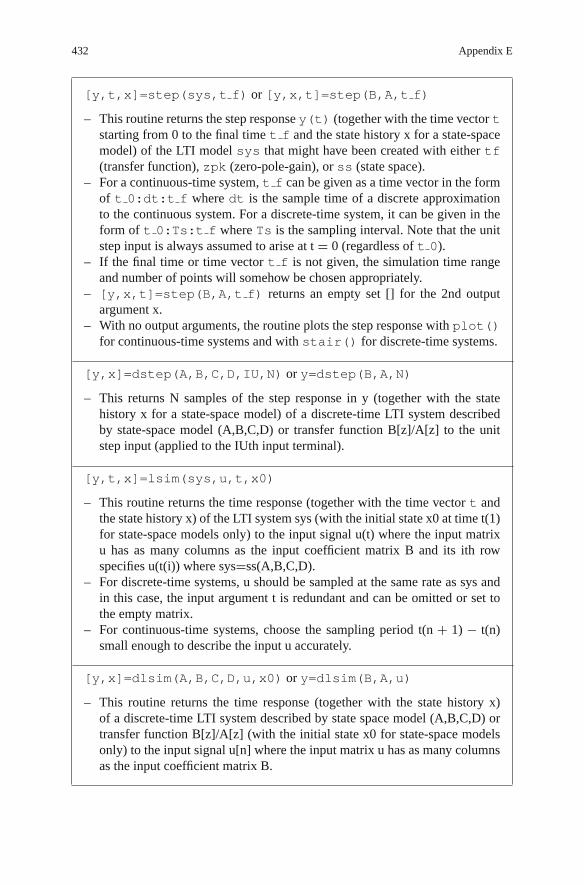
432 Appendix E
[y,t,x]=step(sys,t f) or [y,x,t]=step(B,A,t f)
– This routine returns the step response y(t) (together with the time vector tstarting from 0 to the final time t f and the state history x for a state-spacemodel) of the LTI model sys that might have been created with either tf(transfer function), zpk (zero-pole-gain), or ss (state space).
– For a continuous-time system, t f can be given as a time vector in the formof t 0:dt:t f where dt is the sample time of a discrete approximationto the continuous system. For a discrete-time system, it can be given in theform of t 0:Ts:t f where Ts is the sampling interval. Note that the unitstep input is always assumed to arise at t = 0 (regardless of t 0).
– If the final time or time vector t f is not given, the simulation time rangeand number of points will somehow be chosen appropriately.
– [y,x,t]=step(B,A,t f) returns an empty set [] for the 2nd outputargument x.
– With no output arguments, the routine plots the step response with plot()for continuous-time systems and with stair() for discrete-time systems.
[y,x]=dstep(A,B,C,D,IU,N) or y=dstep(B,A,N)
– This returns N samples of the step response in y (together with the statehistory x for a state-space model) of a discrete-time LTI system describedby state-space model (A,B,C,D) or transfer function B[z]/A[z] to the unitstep input (applied to the IUth input terminal).
[y,t,x]=lsim(sys,u,t,x0)
– This routine returns the time response (together with the time vector t andthe state history x) of the LTI system sys (with the initial state x0 at time t(1)for state-space models only) to the input signal u(t) where the input matrixu has as many columns as the input coefficient matrix B and its ith rowspecifies u(t(i)) where sys=ss(A,B,C,D).
– For discrete-time systems, u should be sampled at the same rate as sys andin this case, the input argument t is redundant and can be omitted or set tothe empty matrix.
– For continuous-time systems, choose the sampling period t(n + 1) − t(n)small enough to describe the input u accurately.
[y,x]=dlsim(A,B,C,D,u,x0) or y=dlsim(B,A,u)
– This routine returns the time response (together with the state history x)of a discrete-time LTI system described by state space model (A,B,C,D) ortransfer function B[z]/A[z] (with the initial state x0 for state-space modelsonly) to the input signal u[n] where the input matrix u has as many columnsas the input coefficient matrix B.
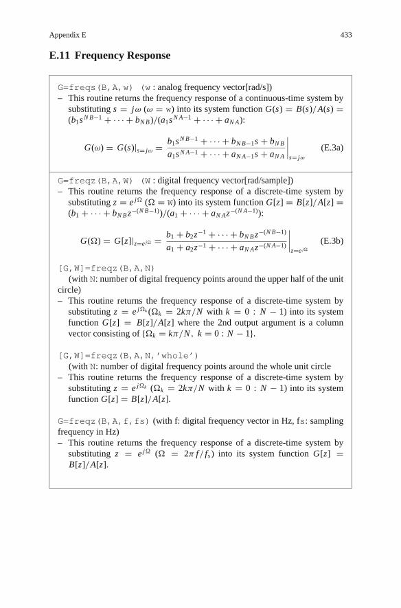
Appendix E 433
E.11 Frequency Response
G=freqs(B,A,w) (w : analog frequency vector[rad/s])– This routine returns the frequency response of a continuous-time system by
substituting s = jω (ω = w) into its system function G(s) = B(s)/A(s) =(b1s N B−1 + · · · + bN B)/(a1s N A−1 + · · · + aN A):
G(ω) = G(s)|s= jω = b1s N B−1 + · · · + bN B−1s + bN B
a1s N A−1 + · · · + aN A−1s + aN A
∣∣∣∣s= jω
(E.3a)
G=freqz(B,A,W) (W : digital frequency vector[rad/sample])– This routine returns the frequency response of a discrete-time system by
substituting z = e jΩ (Ω = W) into its system function G[z] = B[z]/A[z] =(b1 + · · · + bN B z−(N B−1))/(a1 + · · · + aN Az−(N A−1)):
G(Ω) = G[z]|z=e jΩ = b1 + b2z−1 + · · · + bN B z−(N B−1)
a1 + a2z−1 + · · · + aN Az−(N A−1)
∣∣∣∣z=e jΩ
(E.3b)
[G,W]=freqz(B,A,N)(with N: number of digital frequency points around the upper half of the unit
circle)– This routine returns the frequency response of a discrete-time system by
substituting z = e jΩk (Ωk = 2kπ/N with k = 0 : N − 1) into its systemfunction G[z] = B[z]/A[z] where the 2nd output argument is a columnvector consisting of {Ωk = kπ/N , k = 0 : N − 1}.
[G,W]=freqz(B,A,N,’whole’)(with N: number of digital frequency points around the whole unit circle
– This routine returns the frequency response of a discrete-time system bysubstituting z = e jΩk (Ωk = 2kπ/N with k = 0 : N − 1) into its systemfunction G[z] = B[z]/A[z].
G=freqz(B,A,f,fs) (with f: digital frequency vector in Hz, fs: samplingfrequency in Hz)– This routine returns the frequency response of a discrete-time system by
substituting z = e jΩ (Ω = 2π f/ fs) into its system function G[z] =B[z]/A[z].

434 Appendix E
E.12 Filtering
[y,wf]=filter(B,A,x,w0) or[y,wf]=filter(Gd structure,x,w0)
– This routine computes the output y (together with the final condition wf)of the digital filter G[z] = B[z]/A[z] = (b1 + · · · + bN B z−(N B−1))/(a1 +· · · + aN Az−(N A−1)) (described by numerator B and denominator A or a fil-ter structure constructed using dfilt()) to the input x (with the initialcondition w0).
– Let every filter coefficient be divided by a1 for normalization so that we havethe system function of the digital filter as
G[z] = b1 + b2z−1 + · · · + bN B z−(N B−1)
a1 + a2z−1 + · · · + aN Az−(N A−1)
bi /a1→bi=ai /a1→ai
b1 + b2z−1 + · · · + bN B z−(N B−1)
1 + a2z−1 + · · · + aN Az−(N A−1)(E.4)
x [n]
delay
: signal distribution point, : summer
y [n]bN
z–1 z–1 z–1
wN–1[n] w2[n] w1[n]
b2 b1
w2[n–1] w1[n–1]wN–2[n]wN–1[n–1]
bN–1
–aN –a2–aN–1
Fig. E.2 Implementation of an FIR filter in the transposed direct form II structure
The difference equation describing the input-output relationship of the filter
y[n] = −a2 y[n−1]−· · ·−aN A y[n−N A+1]+b1x[n]+· · ·+bN B x[n−N B+1](E.5)
is implemented in the transposed direct form II structure (Fig. E.2) as
y[n] = w1[n − 1] + b1x[n]w1[n] = w2[n − 1] − a2 y[n] + b2x[n]· · · · · · · · · · · · · · · · · · · · · · · · · · · · · · · · · · · ·wN−2[n] = wN−1[n − 1] − aN−1 y[n] + bN−1x[n]wN−1[n] = −aN y[n] + bN x[n]
where N = max(N A, N B) and the initial condition vector w0 oflength N − 1 can be determined from the past output/input by usingw0=filtic(B,A,yp,xp).

Appendix E 435
– When the input x is given as an L × M matrix, filter() operates oneach column of the input matrix. If the initial state wi is nonzero, it must begiven as an (N − 1) × M matrix where N = max(N A, N B). The followingprogram illustrates how to apply it to obtain the output(s) of a filter withsome initial states sample by sample:
Ts=0.001; tt=[0:Ts:0.2]; x= [sin(2*pi*20*tt); cos(2*pi*50*tt)]; x=x.’;B=[1 1]; A=[1 1.5 0.5]; %numerator/denominator of filter transfer functionNB=length(B); NA=length(A); N=max(NA,NB)-1;[Nx,M]=size(x); wi=zeros(NB-1,M); % input dimension and initial statefor n=1:Nx
if n==1, [yn,wi]= filter(B,A,[zeros(1,M); x(n,:)],wi);else [yn,wi]= filter(B,A,[x([n-1 n],:)],wi);endy(n,:) = yn(end,:);
end
function [y,y0]=filterb(B, A, x, y0)% Input: x= [x(-NB+1),..,x(0),x(1),..,x(n)]: the past/future input% y0= [y(-NA+1),..,y(-1)]: the past output% Output: y= [y(0),y(1),..,y(n)]: the output% y0= [y(n-NA+1),..,y(n)]: the last output% to be used for successive processing of the same filterif nargin<4, y0=[]; endNA= length(A);A1=A;for i=1:NAif A(i)==0, A1=A(i+1:NA); else break; end
endA=A1; NA= length(A); NB= length(B); N= NA-1; % the order of filterNy0= length(y0);if length(x)<NB, x=[x zeros(1,NB-length(x))]; endif Ny0<=N %the initial values of the outputy0= [zeros(1,N-Ny0) y0];elseif Ny0>Ny0= y0(Ny0-N+1:Ny0);
endA1= A(NA:-1:2);if A(1)˜=1, B= B/A(1); A1= A1/A(1); endfor n= 1: length(x)-NB+1
y(n)= B*x(n+NB-1:-1:n)’;if NA>1, y(n)= y(n)-A1*y0’; endy0= [y0(2:N) y(n)];
end
Y=filter2(B,X)
– This routine computes the output Y of the 2-D (two-dimensional) FIR filterdescribed by matrix B where most of its work is done by using conv2.

436 Appendix E
E.13 Filter Design
E.13.1 Analog Filter Design
[N,wc]=buttord(wp,ws,Rp,As,’s’)
– This routine selects the lowest order N and cutoff frequency wc of analogButterworth filter that has the passband ripple<= Rp[dB] and stopbandattenuation>= As[dB] for the passband edge frequency wp[rad/s] andstopband edge frequency ws[rad/s]. (Sect. 7.1)
– The cutoff frequency is the frequency at which the magnitude response is1/
√2.
– Note that for BPF/BSF, the passband edge frequency wp and stopband edgefrequency ws should be given as two-element vectors like [wp1 wp2] and[ws1 ws2].
[B,A]=butter(N,wc,’s’)
– This routine designs an analog Butterworth filter, returning the numera-tor/denominator of system function of designed filter.
– [B,A]=butter(N,wc,’s’) for an analog LPF of order N with cutofffrequency wc[rad/s]
– butter(N,[wc1 wc2],’s’) for an analog BPF of order 2N withpassband wc1 < w < wc2 [rad/s]
– butter(N,[wc1 wc2],’stop’,’s’) for an analog BSF of order 2Nwith stopband wc1 < w < wc2 [rad/s]
– butter(N,wc,’high’,’s’) for an analog HPF of order N with cutofffrequency wc[rad/s]
– Note that N and wc can be obtained from[N,wc]=buttord(wp,ws,Rp,As,’s’).
[B,A]=cheby1(N,Rp,wpc,’s’)
– This routine designs an analog Chebyshev type I filter with passband rip-ple Rp[dB] and critical passband edge frequency wpc (Use Rp = 0.5 as astarting point, if not sure).
– Note that N and wpc can be obtained from[N,wpc]=cheby1ord(wp,ws,Rp,As,’s’).
[B,A]=cheby2(N,As,wsc,’s’)
– This routine designs an analog Chebyshev type II filter with stopband atten-uation As[dB] down and critical stopband edge frequency wsc (Use As = 20as a starting point, if not sure).
– Note that N and wsc can be obtained from[N,wsc]=cheby2ord(wp,ws,Rp,As,’s’).

Appendix E 437
[B,A]=ellip(N,Rp,As,wpc,’s’)
– This routine designs an analog Elliptic filter with passband ripple Rp,stopband attenuation As, and critical passband edge frequency wpc (UseRp = 0.5[dB] & As = 20[dB], if unsure).
– Note that N and wpc can be obtained fromellipord(wp,ws,Rp,As,’s’).
E.13.2 Digital Filter Design – IIR (Infinite-duration ImpulseResponse) Filter
[N,fc]=buttord(fp,fs,Rp,As)
– This routine selects the lowest order N and normalized cutoff frequency fc ofdigital Butterworth filter that has passband ripple<= Rp[dB] and stopbandattenuation>= As[dB] for passband edge frequency fp and stopband edgefrequency fs.
– The cutoff frequency is the frequency at which the magnitude response is1/
√2.
– As far as digital filter is concerned, every digital frequency Ωi = ωi T =2π fi T [rad/sample] should be divided by π so that it can be normalizedinto the range [0, 1] where 1.0 corresponds to the digital frequency π
[rad/sample].– Note that for BPF/BSF, the passband edge frequency fp and stopband edge
frequency fs should be given as two-dimensional vectors like [fp1 fp2] and[fs1 fs2].
[B,A]=butter(N,fc)
– This routine designs the system function of digital Butterworth filter.– [B,A]=butter(N,fc): digital LPF of order N with cutoff frequency fc– butter(N,[fc1 fc2]): digital BPF of order 2N with passband fc1 <
f < fc2– butter(N,[fc1 fc2],’stop’): digital BSF of order 2N with stop-
band fc1 < f < fc2– butter(N,fc,’high’): digital HPF of order N with cutoff fre-
quency fc– Note that N and fc can be obtained from[N,fc]=buttord(fp,fs,Rp,As).

438 Appendix E
[B,A]=cheby1(N,Rp,fpc,opt)
– This routine designs a digital Chebyshev type I filter with passband rippleRp[dB] and critical passband edge frequency fpc (Use Rp = 0.5 as a startingpoint, if not sure).
– Note that N and fpc can be obtained from[N,fpc]=cheby1ord(fp,fs,Rp,As).
[B,A]=cheby2(N,As,fsc,opt)
– This routine designs a digital Chebyshev type II filter with stopband attenu-ation As[dB] down and critical stopband edge frequency fsc (Use As = 20as a starting point, if not sure).
– Note that N and fsc can be obtained from[N,fsc]=cheby2ord(fp,fs,Rp,As).
[B,A]=ellip(N,Rp,As,fpc,opt)
– This routine designs a digital elliptic filter with passband ripple Rp, stopbandattenuation As, and critical passband edge frequency fpc (Use Rp = 0.5[dB]and As = 20[dB], if unsure).
– Note that N and fpc can be obtained from ellipord(fp,fs,Rp,As).
E.13.3 Digital Filter Design – FIR (Finite-duration ImpulseResponse) Filter
B=fir1(N,fc,opt)
– This designs a linear-phase FIR filter by using the windowing method.(Sect. 7.2.2.1)
– The normalized cutoff frequency fc must be between 0 and 1, with 1.0 cor-responding to the digital frequency π [rad/sample] or half the sampling rate.
– B=fir1(N,fc) designs an Nth order lowpass FIR filter with linear phaseand returns the (real-valued) filter coefficients in a row vector B of lengthN + 1 where the normalized gain of the filter at fc is −6 dB.
– B=fir1(N,fc,’high’) designs an Nth order highpass FIR filter.– If fc is a two-element vector such as fc = [fc1 fc2], fir1(N,fc)
designs an Nth order BPF with passband fc1 < f < fc2, whilefir1(N,fc,’stop’) designs a bandstop filter.
– If fc is a multi-element vector such as fc = [fc1 fc2 fc3 fc4 . . . fcM], itdesigns an Nth order multi-band filter with bands 0 < f < fc1, fc1 <
f < fc2, . . . , fcM < f < 1. Note that, depending on the value ofa trailing input argument opt = “DC-1” or “DC-0”, it makes the first

Appendix E 439
band a passband or stopband, that is, B=fir1(N,fc,’DC-1’) andB=fir1(N,fc,’DC-0’) make the first band a passband and a stopband,respectively.
– B=fir1(N,fc,WND) designs an Nth order FIR filter using the N + 1length vector WND to window the impulse response. If empty or omit-ted (by default), fir1 uses a Hamming window of length N + 1. Otherwindows such as Boxcar, Hann, Bartlett, Blackman, Kaiser, and Cheb-win can be specified with an optional trailing argument. For example,fir1(N,fc,chebwin(N+1,R)) uses a Chebyshev window.
– For filters with a non-zero gain at fs/2 (half the sampling rate correspondingto the digital frequency π ), e.g., HPF and BSF, N must be even. If N is anodd number for HPF or BSF, it will be incremented by one to make the filterorder even and the window length will be N + 2.
– By default, the filter is scaled so that the center of the first passband has a unitmagnitude after windowing. To prevent this scaling, use a trailing ’noscale’argument as illustrated byfir1(N,fc,’high’,’noscale’) andfir1(N,fc,WND,’noscale’).
B=fir2(N,F,A)
– This designs a FIR filter by using the frequency sampling method. (SeeExample 7.4)
– B=fir2(N,F,A) designs an Nth order FIR filter with the frequencyresponse specified by frequency vector F and amplitude vector A, andreturns the filter coefficients in a row vector B of length N + 1.
– Vectors F and A specify the frequency and magnitude breakpoints such thatplot(F,A) would show a plot of the desired frequency response, where thefrequencies in F must be between 0.0 < F < 1.0 (with 1.0 correspondingto half the sample frequency) and must also be in increasing order startingfrom 0.0 and ending with 1.0.
– The filter B is real, and has linear phase, consisting of symmetric coefficientsobeying B(k) = B(N + 2 − k) for k = 1, 2, . . . , N + 1.
– By default, fir2 windows the impulse response with a Hamming window.Other windows can be specified with an optional trailing argument.
– For filters with a non-zero gain at fs/2 (half the sampling rate correspondingto the digital frequency π ), e.g., HPF and BSF, N must be even. If N is anodd number for HPF or BSF, it will be incremented by one to make the filterorder even and the window length will be N + 2.
B=firpm (N, F, A)
– This designs a Parks-McClellan optimal equiripple FIR filter with desiredfrequency response.
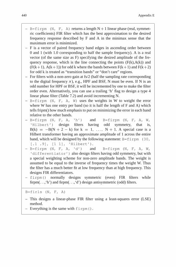
440 Appendix E
– B=firpm (N, F, A) returns a length N + 1 linear phase (real, symmet-ric coefficients) FIR filter which has the best approximation to the desiredfrequency response described by F and A in the minimax sense that themaximum error is minimized.
– F is a vector of paired frequency band edges in ascending order between0 and 1 (with 1.0 corresponding to half the sample frequency). A is a realvector (of the same size as F) specifying the desired amplitude of the fre-quency response, which is the line connecting the points (F(k),A(k)) and(F(k+1), A(k+1)) for odd k where the bands between F(k+1) and F(k+2)for odd k is treated as “transition bands” or “don’t care” regions.
– For filters with a non-zero gain at fs/2 (half the sampling rate correspondingto the digital frequency π ), e.g., HPF and BSF, N must be even. If N is anodd number for HPF or BSF, it will be incremented by one to make the filterorder even. Alternatively, you can use a trailing ‘h’ flag to design a type 4linear phase filter (Table 7.2) and avoid incrementing N.
– B=firpm (N, F, A, W) uses the weights in W to weight the errorwhere W has one entry per band (so it is half the length of F and A) whichtells fripm() how much emphasis to put on minimizing the error in each bandrelative to the other bands.
– B=firpm (N, F, A, ‘h’) and B=firpm (N, F, A, W,‘Hilbert’) design filters having odd symmetry, that is,B(k) = −B(N + 2 − k) for k = 1, . . . , N + 1. A special case is aHilbert transformer having an approximate amplitude of 1 across the entireband, which will be designed by the following statement: B=firpm (30,[.1 .9], [1 1], ‘Hilbert’).
– B=firpm (N, F, A, ‘d’) and B=firpm (N, F, A, W,‘differentiator’) also design filters having odd symmetry, but witha special weighting scheme for non-zero amplitude bands. The weight isassumed to be equal to the inverse of frequency times the weight W. Thusthe filter has a much better fit at low frequency than at high frequency. Thisdesigns FIR differentiators.
– firpm() normally designs symmetric (even) FIR filters whilefirpm(. . .,‘h’) and firpm(. . .,‘d’) design antisymmetric (odd) filters.
B=firls (N, F, A)
– This designs a linear-phase FIR filter using a least-squares error (LSE)method.
– Everything is the same with firpm().

Appendix E 441
B=fircls (N, F, A, ub, lb)
– This designs a length N + 1 linear-phase FIR multi-band filter (with the fre-quency response amplitude A upperbounded/lowerbounded by ub/lb) usinga constrained LSE.
– F is a vector of normalized transition frequencies in ascending order from 0to 1 (corresponding to half the sampling rate), whose length is one plus thenumber of bands, i.e., length(A) + 1.
– A, ub, and lb are vectors of length(F)-1 piecewise constant desired frequencyresponse amplitudes and their upper/lower bounds for each band.
(Ex) B=fircls (10, [0 0.4 0.8 1], [0 1 0], [0.02 1.02 0.01],
[−0.02 0.98 −0.01])
B=fircls1 (N, fc, rp, rs, opt)
– This designs a length N + 1 linear-phase FIR LPF/HPF (with the cut-off frequency fc) using a constrained LSE method where rp/rs specify thepassband/stopband ripple, respectively.
– With opt=‘high’, it designs a HPF.
(Ex) B=fircls1 (10, 0.7, 0.02, 0.01, ‘high’)
(cf.) The GUI signal processing tool “sptool” manages a suite of four other GUIs:signal browser, filter designer, fvtool (for filter visualization), and spectrumviewer where “fdatool” is for filter design and analysis.
E.14 Filter Discretization
[Bz,Az]=impinvar (Bs, As, fs, tol)
– This uses the impulse-invariant method (Sect. 6.2.1) to convert a continuous-time system G(s) = B(s)/A(s) into an equivalent discrete-time systemG[z] = B[z]/A[z] such that the impulse response is invariant except forbeing scaled by Ts = 1/fs.
– If you leave out the argument fs or specify it as the empty vector [], itsdefault value 1 Hz will be taken.
– The fourth input argument tol specifies the tolerance to determine whetherpoles are repeated. A larger tolerance increases the likelihood thatimpinvar() interprets closely located poles as multiplicities (repeatedones). The default is 0.001, or 0.1% of a pole’s magnitude. Note that theaccuracy of the pole values is still limited to the accuracy obtainable by theroots() function.

442 Appendix E
[Bz,Az]=bilinear (Bs, As, fs, fp)
– This uses the bilinear transformation (BLT) method (Sect. 6.3.5) to converta continuous-time system G(s) = B(s)/A(s) into its discrete equivalentG[z] = B[z]/A[z] such that the entire LHP on the s-plane maps into theunit circle on the z-plane in one-to-one correspondence.
– The numerator/denominator polynomial vector Bs and As of an analog fil-ter are written in descending powers of s and the numerator/denominatorpolynomial vector Bz and Az of the discrete-time equivalent are written indescending powers of z (ascending powers of z−1).
– The optional parameter fp[Hz] specifies a prewarping match frequency forwhich the frequency responses before and after BLT mapping match exactly.
sysd=c2d (sysc, Ts, method)
– This converts a continuous-time system (transfer) function sysc (that mighthave been created with either tf (transfer function), zpk (zero-pole-gain),or ss (state space)) into an equivalent discrete-time system function sysdwith the sampling interval Ts[s] by using the discretization method amongthe following:
‘zoh’ : Zero-order hold on the inputs (by default) - Sect. 6.2.2‘foh’ : Linear interpolation of inputs (triangle approximation)‘imp’ : Impulse-invariant discretization - Sect. 6.2.1‘tustin’ : Bilinear (Tustin) approximation - Sect. 6.3.5‘prewarp’ : Tustin approximation with frequency prewarping where the
critical frequency Wc (in rad/s) is specified as fourth input,e.g., as sysd = c2d(sysc,Ts,‘prewarp’,Wc)
‘matched’ : Matched pole-zero method (for SISO systems only) –Sect. 6.3.6
[Ad,Bd]=c2d (Ac, Bc, Ts)– This converts a continuous-time state equation x’(t) = Ac∗x(t) + Bc∗u(t)
into the zero-order-hold (z.o.h.) equivalent discrete-time state equation x[n+1] = Ad∗x[n] + Bd∗u[n] with the sampling interval Ts[s]. (Sect. 8.4.1)
sysc=d2c (sysd, method)
– This converts a discrete-time system function into an equivalent continuous-time system function.
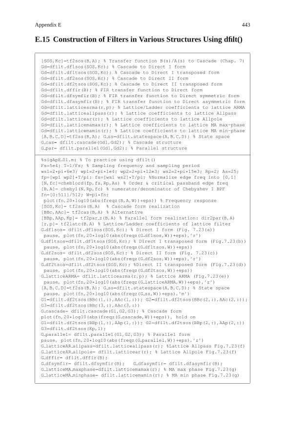
Appendix E 443
E.15 Construction of Filters in Various Structures Using dfilt()
[SOS,Kc]=tf2sos(B,A); % Transfer function B(s)/A(s) to Cascade (Chap. 7)Gd=dfilt.df1sos(SOS,Kc); % Cascade to Direct I formGd=dfilt.df1tsos(SOS,Kc); % Cascade to Direct I transposed formGd=dfilt.df2sos(SOS,Kc); % Cascade to Direct II formGd=dfilt.df2tsos(SOS,Kc); % Cascade to Direct II transposed formGd=dfilt.dffir(B); % FIR transfer function to Direct formGd=dfilt.dfsymfir(B); % FIR transfer function to Direct symmetric formGd=dfilt.dfasymfir(B); % FIR transfer function to Direct asymmetric formGd=dfilt.latticearma(r,p); % Lattice/Ladder coefficients to lattice ARMAGd=dfilt.latticeallpass(r); % Lattice coefficients to lattice AllpassGd=dfilt.latticear(r); % Lattice coefficients to lattice AllpoleGd=dfilt.latticemamax(r); % Lattice coefficients to lattice MA max-phaseGd=dfilt.latticemamin(r); % Lattice coefficients to lattice MA min-phase[A,B,C,D]=tf2ss(B,A); G ss=dfilt.statespace(A,B,C,D); % State spaceG cas= dfilt.cascade(Gd1,Gd2); % Cascade structureG par= dfilt.parallel(Gd1,Gd2); % Parallel structure
%sigApE 01.m: % To practice using dfilt()Fs=5e4; T=1/Fs; % Sampling frequency and sampling periodws1=2*pi*6e3; wp1=2*pi*1e4; wp2=2*pi*12e3; ws2=2*pi*15e3; Rp=2; As=25;fp=[wp1 wp2]*T/pi; fs=[ws1 ws2]*T/pi; %Normalize edge freq into [0,1][N,fc]=cheb1ord(fp,fs,Rp,As) % Order & critical passband edge freq[B,A]= cheby1(N,Rp,fc) % numerator/denominator of Chebyshev I BPFfn=[0:511]/512; W=pi*fn;plot(fn,20*log10(abs(freqz(B,A,W))+eps)) % Frequency response
[SOS,Kc]= tf2sos(B,A) % Cascade form realization[BBc,AAc]= tf2cas(B,A) % Alternative[BBp,AAp,Kp]= tf2par z(B,A) % Parallel form realization: dir2par(B,A)[r,p]= tf2latc(B,A) % Lattice/Ladder coefficients of lattice filterG df1sos= dfilt.df1sos(SOS,Kc); % Direct I form (Fig. 7.23(a))pause, plot(fn,20*log10(abs(freqz(G df1sos,W))+eps),’r’)
G df1tsos=dfilt.df1tsos(SOS,Kc); % Direct I transposed form (Fig.7.23(b))pause, plot(fn,20*log10(abs(freqz(G df1tsos,W))+eps))
G df2sos= dfilt.df2sos(SOS,Kc); % Direct II form (Fig. 7.23(c))pause, plot(fn,20*log10(abs(freqz(G df2sos,W))+eps),’r’)
G df2tsos=dfilt.df2tsos(SOS,Kc); %Direct II transposed form (Fig.7.23(d))pause, plot(fn,20*log10(abs(freqz(G df2tsos,W))+eps))
G latticeARMA= dfilt.latticearma(r,p); % Lattice ARMA (Fig.7.23(e))pause, plot(fn,20*log10(abs(freqz(G latticeARMA,W))+eps),’r’)
[A,B,C,D]=tf2ss(B,A); G ss=dfilt.statespace(A,B,C,D); % State spacepause, plot(fn,20*log10(abs(freqz(G ss,W))+eps),’m’)
G1=dfilt.df2tsos(BBc(1,:),AAc(1,:)); G2=dfilt.df2tsos(BBc(2,:),AAc(2,:));G3=dfilt.df2tsos(BBc(3,:),AAc(3,:))G cascade= dfilt.cascade(G1,G2,G3); % Cascade formplot(fn,20*log10(abs(freqz(G cascade,W))+eps)), hold onG1=dfilt.df2tsos(BBp(1,:),AAp(1,:)); G2=dfilt.df2tsos(BBp(2,:),AAp(2,:))G3=dfilt.df2tsos(Kp,1);G parallel= dfilt.parallel(G1,G2,G3); % Parallel formpause, plot(fn,20*log10(abs(freqz(G parallel,W))+eps),’r’)G latticeAR allpass=dfilt.latticeallpass(r); %Lattice Allpass Fig.7.23(f)G latticeAR allpole= dfilt.latticear(r); % Lattice Allpole Fig.7.23(f)G dffir= dfilt.dffir(B);G dfsymfir= dfilt.dfsymfir(B); G dfasymfir= dfilt.dfasymfir(B);G latticeMA maxphase=dfilt.latticemamax(r); % MA max phase Fig.7.23(g)G latticeMA minphase= dfilt.latticemamin(r); % MA min phase Fig.7.23(g)

444 Appendix E
function [BB,AA,K]=tf2par s(B,A)% Copyleft: Won Y. Yang, [email protected], CAU for academic use onlyEPS= 1e-8;B= B/A(1); A= A/A(1);I= find(abs(B)>EPS); K= B(I(1)); B= B(I(1):end);p= roots(A); p= cplxpair(p,EPS); Np= length(p);NB= length(B); N= length(A); M= floor(Np/2);for m=1:M
m2= m*2; AA(m,:) = [1 -p(m2-1)-p(m2) p(m2-1)*p(m2)];endif Np>2*M
AA(M+1,:)= [0 1 -p(Np)]; % For a single poleendM1= M+(Np>2*M); b= [zeros(1,Np-NB) B]; KM1= K/M1;% In case B(s) and A(s) has the same degree, we let all the coefficients% of the 2ˆ{nd}-order term in the numerator of each SOS be Bi1=1/M1:if NB==N, b= b(2:end); endfor m=1:M1
polynomial = 1; m2=2*m;for n=1:M1
if n˜=m, polynomial = conv(polynomial,AA(n,:)); endendif m<=M
if M1>M, polynomial = polynomial(2:end); endif NB==N, b = b - [polynomial(2:end)*KM1 0 0]; endAc(m2-1,:) = [polynomial 0];Ac(m2,:) = [0 polynomial];elseif NB==N, b = b - [polynomial(2:end)*KM1 0]; endAc(m2-1,:) = polynomial;
endendBc = b/Ac; Bc(find(abs(Bc)<EPS)) = 0;for m=1:M1
m2= 2*m;if m<=M
BB(m,:) = [0 Bc(m2-1:m2)]; if NB==N, BB(m,1) = KM1; endelseBB(m,:) = [0 0 Bc(end)]; if NB==N, BB(m,2) = KM1; end
endend
function [BB,AA,K]=tf2par z(B,A)% Copyleft: Won Y. Yang, [email protected], CAU for academic use onlyif nargin<3, IR =0; end % For default, inverse z-transform styleEPS= 1e-8; %1e-6;B= B/A(1); A= A/A(1);I= find(abs(B)>EPS); B= B(I(1):end);if IR==0, [z,p,K]= residuez(B,A); else [z,p,K]= residue(B,A); endm=1; Np=length(p); N=ceil(Np/2);for i=1:N
if abs(imag(p(m)))<EPS % Real poleif m+1<=Np & abs(imag(p(m+1)))<EPS % Subsequent real poleif abs(p(m)-p(m+1))<EPS % Double pole
BB(i,:)= [z(m)+z(m+1) -z(m)*p(m) 0];AA(i,:)= [1 -2*p(m) p(m)ˆ2]; m=m+2;
elseif m+2<=Np&abs(p(m+1)-p(m+2))<EPS %Next two poles are double
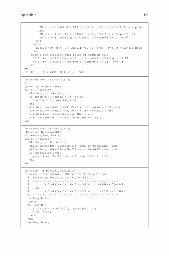
Appendix E 445
BB(i,:)=[0 z(m) 0]; AA(i,:)=[0 1 -p(m)]; m=m+1; % Single poleelseBB(i,:)= [real([z(m)+z(m+1) -z(m)*p(m+1)-z(m+1)*p(m)]) 0];AA(i,:)= [1 real([-p(m)-p(m+1) p(m)*p(m+1)])]; m=m+2;
endelseBB(i,:)=[0 z(m) 0]; AA(i,:)=[0 1 -p(m)]; m=m+1; % Single poleend
else % Two distinct real poles or Complex poleBB(i,:)= [real([z(m)+z(m+1) -z(m)*p(m+1)-z(m+1)*p(m)]) 0];AA(i,:)= [1 real([-p(m)-p(m+1) p(m)*p(m+1)])]; m=m+2;
endendif IR∼=0, BB(:,2:3)= BB(:,1:2); end
function y=filter cas(B,A,x)y=x;[Nsection,NB]=size(B);for k=1:Nsection
Bk= B(k,:); Ak= A(k,:);if abs(B(k,1))+abs(A(k,1))<1e-10
Bk= B(k,2:3); Ak= A(k,2:3);end%if B(k,3)==0&A(k,3)==0, Bk=B(k,1:2); Ak=A(k,1:2); end%if B(k,2)==0&A(k,2)==0, Bk=B(k,1); Ak=A(k,1); end%if Bk(1)==0; Bk=Bk(2:length(Bk)); endy=filterb(Bk,Ak,[zeros(1,length(Bk)-1) y]);
end
function y=filter par(B,A,x)[Nsection,NB]=size(B);y= zeros(1,length(x));for k=1:Nsection
Bk= B(k,:); Ak= A(k,:);while length(Bk)>1&abs(Bk(1))<eps, Bk=Bk(2:end); endwhile length(Ak)>1&abs(Ak(1))<eps, Ak=Ak(2:end); endif sum(abs(Bk))>eps
y=y+filterb(Bk,Ak,[zeros(1,length(Bk)-1) x]);end
end
function [r,p]=tf2latc my(B,A)if nargin>1&length(A)>1 %Recursive Lattice Filter
% IIR System Function to Lattice Filter% ****************************************************% B(1)+B(2)*zˆ-1 +B(3)*zˆ-2 +.....+B(NB)*zˆ(-NB+1)% G[z] = ---------------------------------------------% A(1)+A(2)*zˆ-1 +A(3)*zˆ-2 +......+A(NA)*zˆ(-NA+1)% ****************************************************N= length(A);AA= A;for k=1:N-1
if abs(AA(k))<.0000001, A= AA(k+1: N);else break;end
endN= length(A);

446 Appendix E
if N<=1, error(’LATTICED: length of polynomial is too short!’); endBB= B;NB= length(B);for k=1:NB-1
if abs(BB(k))<.0000001, B= BB(k+1: NB);else break;end
endif length(B) ˜= N
error(’tf2latc my: lengths of polynomials B and A do not agree!’);endS= B/A(1); V= A/A(1);for i=N:-1:2
p(i)= S(i); ri1= V(i);W(1:i)= V(i:-1:1);if abs(ri1)>=.99999
error(’tf2latc my: ri1= V(i) is too large to maintain stability!’);endV(1:i)= (V(1:i)-ri1*W(1:i))/(1-ri1*ri1);r(i-1)= ri1;S(1:i)= S(1:i) -p(i)*W(1:i);
endp(1)= S(1);if nargout==0
fprintf(’\n\t Recursive Lattice Filter Coefficients\n’);for i=1:length(r), fprintf(’ r(%1d)=%7.4f’, i, r(i)); endfprintf(’\n’);for i=1:length(p), fprintf(’ p(%1d)=%7.4f’, i, p(i)); endfprintf(’\n’);
endelse %Nonrecursive Lattice Filter
% FIR System Function --> Nonrecursive Lattice-II Filter% ****************************************************% G[z]= B(1)+B(2)*zˆ-1 +B(3)*zˆ-2 +.....+B(NB)*zˆ(-NB+1)% ****************************************************N= length(B);BB= B;for k=1:N-1
if abs(BB(k))<.0000001, B= BB(k+1: N);else break;end
endN= length(B);if N<=1, error(’tf2latc my: length of polynomial is too short!’); endV= B/B(1);for i=N:-1:2
ri1= V(i);W(1:i)= V(i:-1:1);if abs(abs(ri1)-1)<.001 %Nonrecursive Lattice cannot be unstable
ri1 =ri1/abs(ri1)*.99;endV(1:i)= (V(1:i)-ri1*W(1:i))/(1-ri1*ri1);r(i-1)= ri1;
endif nargout==0
fprintf(’\n\t Nonrecursive Lattice Filter Coefficients\n’);for i=1:length(r), fprintf(’ r(%1d)=%7.4f’, i, r(i)); end

Appendix E 447
fprintf(’\n’);end
end
function [y,w]=filter latc r(r,p,x,w)%hopefully equivalent to latcfilt() inside MATLAB%w contains the past history of internal state ..,w(n-1), w(n)%1-step Lattice filtering the input x to yield the output y and update wN= length(r); % the order of the lattice filterif length(p)˜= N+1
error(’LATTICEF: length(p) must equal length(r)+1!’);endif nargin<4, w=[]; endif length(w)<N
w=[zeros(1,N-length(w)) w];endfor n=1:length(x)
vi=x(n); %Current Inputfor i=N:-1:1
vi= vi -r(i)*w(i); w(i+1)= w(i) +r(i)*vi;endw(1)= vi;y(n)= p(:).’*w(:);
end
function [y,w]=filter latc nr(r,x,w)% hopefully equivalent to latcfilt() inside MATLAB% w contains the past history of internal state...,w(n-1), w(n)%1-step Lattice filtering the input x to yield the output y and update wN= length(r); % the order of the lattice filterif nargin<3, w=[]; endif length(w)<N
w=[zeros(1,N-length(w)) w];endfor n=1:length(x)
vi= x(n)+r*w(1:N)’;y(n)= vi;for i=N:-1:1
vi= vi -r(i)*w(i); w(i+1)= w(i) +r(i)*vi;endw(1)= x(n);
end
E.16 System Identification from Impulse/Frequency Response
[B,A]=prony (g, NB, NA)
– This identifies the system function
G[z] = B[z]
A[z]= b1 + b2z−1 + · · · + bN B+1z−N B
a1 + a2z−1 + · · · + aN A+1z−N A(E.6)
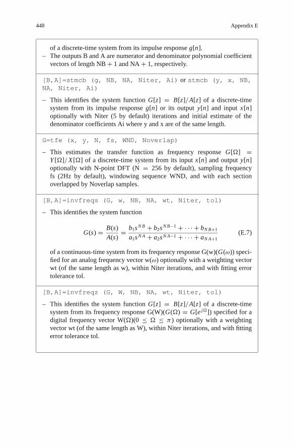
448 Appendix E
of a discrete-time system from its impulse response g[n].– The outputs B and A are numerator and denominator polynomial coefficient
vectors of length NB + 1 and NA + 1, respectively.
[B,A]=stmcb (g, NB, NA, Niter, Ai) or stmcb (y, x, NB,NA, Niter, Ai)
– This identifies the system function G[z] = B[z]/A[z] of a discrete-timesystem from its impulse response g[n] or its output y[n] and input x[n]optionally with Niter (5 by default) iterations and initial estimate of thedenominator coefficients Ai where y and x are of the same length.
G=tfe (x, y, N, fs, WND, Noverlap)
– This estimates the transfer function as frequency response G[Ω] =Y [Ω]/X [Ω] of a discrete-time system from its input x[n] and output y[n]optionally with N-point DFT (N = 256 by default), sampling frequencyfs (2Hz by default), windowing sequence WND, and with each sectionoverlapped by Noverlap samples.
[B,A]=invfreqs (G, w, NB, NA, wt, Niter, tol)
– This identifies the system function
G(s) = B(s)
A(s)= b1s N B + b2s N B−1 + · · · + bN B+1
a1s N A + a2s N A−1 + · · · + aN A+1(E.7)
of a continuous-time system from its frequency response G(w)(G(ω)) speci-fied for an analog frequency vector w(ω) optionally with a weighting vectorwt (of the same length as w), within Niter iterations, and with fitting errortolerance tol.
[B,A]=invfreqz (G, W, NB, NA, wt, Niter, tol)
– This identifies the system function G[z] = B[z]/A[z] of a discrete-timesystem from its frequency response G(W)(G(Ω) = G[e jΩ]) specified for adigital frequency vector W(Ω)(0 ≤ Ω ≤ π ) optionally with a weightingvector wt (of the same length as W), within Niter iterations, and with fittingerror tolerance tol.

Appendix E 449
E.17 Partial Fraction Expansion and (Inverse)Laplace/z-Transform
[r,p,k]=residue (B,A) or [B,A]=residue (r, p, k)
– This converts a rational function B(s)/A(s), i.e., a ratio of numera-tor/denominator polynomials to partial fraction expansion form (or pole-residue representation), and back again.
B(s)
A(s)= b1s N B−1 + b2s N B−2 + · · · + bN B
a1s N−1 + a2s N−2 + · · · + aN
�(
N−1−L∑n=1
rn
s − pn
)+ rN−L
s − p+ · · · + rN−1
(s − p)L+ k(s) (E.8)
where the numerator vector r and pole vector p are column vectors and thequotient polynomial coefficient vector k is a row vector.
[r,p,k]=residuez (B,A) or [B,A]=residuez (r,p,k)
– This converts a rational function B[z]/A[z], i.e., a ratio of numera-tor/denominator polynomials to partial fraction expansion form (or pole-residue representation), and back again.
B[z]
A[z]= b1 + b2z−1 + · · · + bN B z−(N B−1)
a1 + a2z−1 + · · · + aN z−(N−1)
�(
N−1−L∑n=1
rnz
z − p
)+ rN−L z
z − p+ · · · + rN−1zL
(z − p)L+ k(z) (E.9)
where the numerator vector r and pole vector p are column vectors and thequotient polynomial coefficient vector k is a row vector.
Xs=laplace (xt) and xt=ilaplace (Xs)
– These MATLAB commands compute the symbolic expressions for theLaplace transform X (s) = L{x(t)} of a symbolic function in t and theinverse Laplace transform x(t) = L−1{X (s)} of a symbolic function in s,respectively.
Xz=ztrans (xn) and xn=iztrans (Xz)
– These MATLAB commands compute the symbolic expressions for thez -transform X [z] = Z{x[n]} of a symbolic function in n and the inversez -transform x[n] = Z−1{X [z]} of a symbolic function in z, respectively.
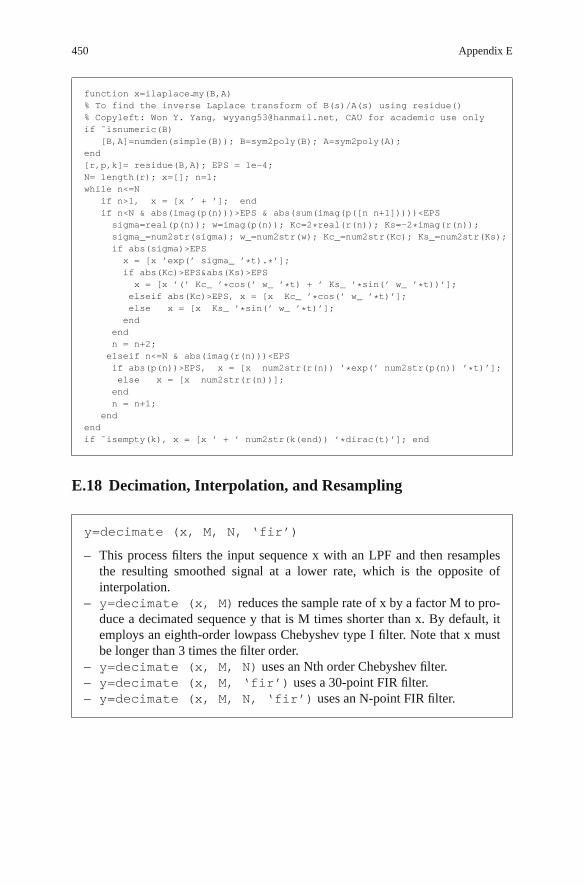
450 Appendix E
function x=ilaplace my(B,A)% To find the inverse Laplace transform of B(s)/A(s) using residue()% Copyleft: Won Y. Yang, [email protected], CAU for academic use onlyif ˜isnumeric(B)
[B,A]=numden(simple(B)); B=sym2poly(B); A=sym2poly(A);end[r,p,k]= residue(B,A); EPS = 1e-4;N= length(r); x=[]; n=1;while n<=N
if n>1, x = [x ’ + ’]; endif n<N & abs(imag(p(n)))>EPS & abs(sum(imag(p([n n+1]))))<EPSsigma=real(p(n)); w=imag(p(n)); Kc=2*real(r(n)); Ks=-2*imag(r(n));sigma_=num2str(sigma); w_=num2str(w); Kc_=num2str(Kc); Ks_=num2str(Ks);if abs(sigma)>EPSx = [x ’exp(’ sigma_ ’*t).*’];if abs(Kc)>EPS&abs(Ks)>EPSx = [x ’(’ Kc_ ’*cos(’ w_ ’*t) + ’ Ks_ ’*sin(’ w_ ’*t))’];elseif abs(Kc)>EPS, x = [x Kc_ ’*cos(’ w_ ’*t)’];else x = [x Ks_ ’*sin(’ w_ ’*t)’];
endendn = n+2;elseif n<=N & abs(imag(r(n)))<EPSif abs(p(n))>EPS, x = [x num2str(r(n)) ’*exp(’ num2str(p(n)) ’*t)’];else x = [x num2str(r(n))];endn = n+1;
endendif ˜isempty(k), x = [x ’ + ’ num2str(k(end)) ’*dirac(t)’]; end
E.18 Decimation, Interpolation, and Resampling
y=decimate (x, M, N, ‘fir’)
– This process filters the input sequence x with an LPF and then resamplesthe resulting smoothed signal at a lower rate, which is the opposite ofinterpolation.
– y=decimate (x, M) reduces the sample rate of x by a factor M to pro-duce a decimated sequence y that is M times shorter than x. By default, itemploys an eighth-order lowpass Chebyshev type I filter. Note that x mustbe longer than 3 times the filter order.
– y=decimate (x, M, N) uses an Nth order Chebyshev filter.– y=decimate (x, M, ‘fir’) uses a 30-point FIR filter.– y=decimate (x, M, N, ‘fir’) uses an N-point FIR filter.

Appendix E 451
y=interp (x, M, L, fc)
– This inserts zeros into the input sequence x and then apply an LPF.– y=interp (x,M) increases the sampling rate of x by a factor of M to
produce an interpolated sequence y that is M times longer than x.– y=interp(x,M,L,fc) specifies L (= 4 by default) for filter length and
fc (= 0.5 by default) for normalized cut-off frequency.– [y,B]=interp(x,M,L,fc) returns a vector B of length 2∗L∗M + 1
containing the filter coefficients used for the interpolation.
y=upfirdn(x,B,Mi,Md)
– This can be used to change the sampling rate by a rational factor.– It upsamples x by Mi (i.e., inserts (Mi-1) zeros between samples), applies the
FIR filter B, and downsamples the output by Md (i.e., throws away (Md-1)samples between samples).
– The default values of Mi and Md are 1.
y=resample(x,Mi,Md,B)
– This can be used to change the sampling rate by a rational factor.– y=resample(x,Mi,Md) resamples x at Mi/Md times the original sam-
pling rate, using a polyphase filter implementation where Mi and Md mustbe positive integers. The length of y will be ceil(length(x)∗Mi/Md). If x is amatrix, resample() works down the columns of x.
– It applies an anti-aliasing (lowpass) FIR filter (designed using firls() with aKaiser window) to x during the resampling process.
– y=resample(x,Mi,Md,B) filters x using a FIR filter with coeffi-cients B.
– y=resample(x,Mi,Md,N) uses a weighted sum of 2∗N∗
max (1, Md/Mi) samples of x to compute each sample of y. Since thelength of the FIR filter used by resample() is proportional to N(= 10 bydefault), you can increase N to get better accuracy at the expense of a longercomputation time. If you let N = 0, a nearest neighbor interpolation isperformed so that the output y(n) is x(round((n − 1)∗Md/Mi) + 1) wherey(n) = 0 if round((n − 1)∗Md/Mi) + 1 > length(x)).
– y=resample(x,Mi,Md,N,beta) uses beta as the design parameter forthe Kaiser window used to design the filter where its default value is 5.
– [y,B]=resample(x,Mi,Md) returns the filter coefficient vector Bapplied to x during the resampling process (after upsampling).
– If x is a matrix, the routine resamples the columns of x.
y=detrend(x)
– y=detrend(x) removes the best straight-line fit from vector x.– y=detrend(x,0) removes the mean value from vector x.

452 Appendix E
E.19 Waveform Generation
chirp(t,f0,t1,f1,’type’) swept-frequency cosine generatorpulstran(t,D,pulse) pulse train generatorrectpuls(t,D) sampled aperiodic rectangular pulse generatorsquare(t,D), sawtooth(t,D) square, sawtooth/triangular wave generatortripuls(t,D,skew) sampled aperiodic triangular pulse generator
E.20 Input/Output through File
% input output data.mclearx=[1 2]; y=[3 4 5];save sig x y % save x and y in a MATLAB data file ’sig.mat’clear(’y’)display(’After y has been cleared, does y exist?’)if (exist(’y’)˜=0), disp(’Yes’), yelse disp(’No’)
endload sig y % read y from the MATLAB data file ’sig.mat’disp(’After y has been loaded the file sig.mat, does y exist?’)if isempty(’y’), disp(’No’), else disp(’Yes’), y, endfprintf(’x(2)=%5.2f \n’, x(2))save y.dat y /ascii % save y into the ASCII data file ’y.dat’% The name of the ASCII data file must be the same as the variable name.load y.dat % read y from the ASCII data file ’y.dat’str=’prod(y)’; % ready to compute the produce of the elements of yeval(str) % evaluate the string expression ’prod(y)’

Appendix FSimulink R©
According to the MATLAB documentation [W-5], Simulink R© is software for mod-eling, simulating, and analyzing dynamic systems. It supports linear and nonlinearsystems, modeled in continuous time, sampled time, or a hybrid of the two. Sys-tems can be multirate, i.e., have different parts that are sampled or updated atdifferent rates.
Simulink R© provides a graphical user interface (GUI) for building models asblock diagrams, using click-and-drag mouse operations. Simulink includes a com-prehensive block library of sinks, sources, linear and nonlinear components, andconnectors. Models are hierarchical, so you can build models using both top-downand bottom-up approaches. You can view the system at a high level, then double-click blocks to go down through the levels to see increasing levels of model detail.This approach provides insight into how a model is organized and how its partsinteract.
After you define a model, you can simulate it either from the Simulink menusor by entering commands in the MATLAB R© Command Window. The menus areconvenient for interactive work, while the command line is useful for runninga batch of simulations with a parameter swept across a range of values. Usingscopes and other display blocks, you can see the simulation results while the sim-ulation runs. The simulation results can be put in the MATLAB workspace forpostprocessing and visualization. MATLAB R© and Simulink R© are integrated sothat you can simulate, analyze, and revise your models in either environment atany point.
To start Simulink, you must first start MATLAB. Consult your MATLAB docu-mentation for more information. You can then start Simulink in two ways:
• Click the Simulink icon on the MATLAB toolbar.• Type “simulink” (without the quotation marks) at the MATLAB prompt (like
“>>”) in the MATLAB Command Window or use the “sim()” command insidea MATLAB program.
On Microsoft Windows platforms, starting Simulink displays the Simulink LibraryBrowser as depicted in Fig. F.1. The Library Browser displays a tree-structuredview of the Simulink block libraries installed on your system, from which you can
453

454 Appendix F
Fig. F.1 Simulink Library Browser window

Appendix F 455
copy and move (click/drag) the blocks into a model window and build models. Theprocedure of creating or editing a Simulink model is as follows:
– A new empty model file (window) can be created by selecting File/New menuor clicking “Create a new model” button on the library browser’s toolbar. Anexisting one can be opened by selecting File/Open menu or clicking the Openbutton on the library browser’s toolbar and then choosing/entering the file namefor the model to edit.
– Copy and move (click/drag) the blocks you want into the model window.– Connect the blocks by clicking at an (input/output) point of a block and drag to
an (output/input) point of another block.– To draw a branch line, position the pointer at a point on the existing line (wire),
press and hold down the CTRL key, press the mouse button, and then drag thepointer to another point.
To simulate the created/edited Simulink model, select the Simulation/Configuration Parameters menu (in the model window) to open the ConfigurationParameters window in which you can set the simulation parameters including thestart/final(stop) times, and then press the CTRL + T key (on the keyboard) or selectthe Simulation/Start menu on the toolbar of the model window. To see the simulationresults, double-click the Scope block.
Figures F.2 and F.3 show the Signal Processing and Communication Blocksets,which enables you to design and prototype various signal processing and commu-nication systems using key signal processing algorithms and components in theSimulink R© block format.
(cf.) If you see an error message that a Simulink model file cannot be savedbecause of character encoding problem, keep the erroneous part of the modelfile in mind, click OK to close the error message dialog block, use a texteditor to modify the erroneous part in the designated file named “∗∗∗.err”,and then save it with the extension name “mdl” instead of “err” so that it canbe opened in another Simulink session.

456 Appendix F
Signal Processing Blockset
EstimationLinear Prediction: Autocorrelation LPC, Levinson-Durbin, LPC to LSF/LSP Conversion
Adaptive Filters: Block LMS Filter, Kalman Adaptive Filter, LMS Filter, RLS FilterFiltering Designs: Analog Filter Design, Digital Filter, Digital Filter Design, Filter Realization WizardMultirate Filters: CIC Decimation/Interpolation, Dyadic Analysis/Synthesis Filter Bank
FIR Decimation/Interpolation, FIR Rate ConversionTwo-Channel Analysis/Synthesis Subband Filter
Math Operations: Complex Exponential, Cumulative Product/SumDifference, Normalization, dB Conversion, dB Gain
Matrices and LInear Algebra:
Linear System Solvers: Backward/Forward Substitution, Levinson-Durbin
Polynomial Functions: Least Squares Polynomial Fit, Polynomial Evaluation Polynomial Stability Test
– Windows (WIN32): From Wave Device/File, To Wave Device/File
Cholesky/LDL/LU/QR/SVD Solver
Matrix Factorizations: Cholesky/LDL/LU/QR/SVD Factorization
Matrix Inverses: Cholesky/LDL/LU/Pseudo Inverse
Matrix Operations: Identity Matrix, Constant Diagonal Matrix, Create Diagonal Matrix Extract Diagonal/Triangular, Overwrite Values, Reciprocal Condition Matrix Concatenation/Product/Scaling/Square/Sum/Multiply/Transpose Matrix 1-Norm, Permute Matrix, Submatrix, Toeplitz
LSF/LSP to LPC Conversion, LPC to/from RC, Autocorrelation, Cepstral Coefficients
Parametric Estimation: Burg AR Estimator, Covariance AR Estimator, Yule-Walker AR EstimatorPower Spectrum Estimation: Burg Method, Covariance Method; Magnitude FFT, Periodogram, Yule-Walker Method
Filtering
Math Functions
Platform Specific I/Q
Quantizers : Quantizer, Uniform Encoder/Decoder
Buffers: Buffer, Delay Line, Triggered Delay Line, Queue, Stack, Unbuffer
Indexing: Selector, Multiport Selector, Variable Selector, Flip, Submatrix, Overwrite Values
Signal Attributes: Check Signal Attributes, Convert 1-D to 2-D, Convert 2-D to 1-DDate Type Conversion, Frame Status Conversion, Inherity Complexity
Switches and Counters: Counter, Edge Detector, Event-Count ComparatorMultiphase Clock, N-Sample Enable, N-Sample Switch
Convolution, Downsample, Upsample, Interpolation, Unwrap, Window FunctionPad, Zero-Pad, Repeat, S/H, Integer Delay, Variable Integer/Fractional Delay
: Autocorrelation, Correlation, Detrend, Histogram, Maximum, Minimum, Mean, Median, RMS, Standard Deviation, Variance, Sort
: Analytic Signal, Real/Complex Cepstrum DCT, DWT, FFT, IDCT, IDWT, IFFT, Magnitude FFT
: Display, Matrix Viewer, Spectrum Scope, Time Scope, Vector Scope Signal To Workspace, Triggered To Workspace
: Chirp, Constant Ramp, Discrete Impulse, DSP Constant, Sine Wave, Random Source Identity Matrix, Constant Diagonal Matrix, Multiphase Clock, N-Sample Enable Signal From Workspace, Triggered Signal From Workspace
Signal Management
Signal Operation
Statistics
Transforms
DSP Sinks
DSP Sources
Fig. F.2 Signal Processing Blockset available in the Simulink Library Browser window

Appendix F 457
Communication Blockset
Integrate and Dump, Windowed Integrator, ...
Insert Zero (Depuncture), Puncture, ...
Integrators:
Channels
Basic Comm Functions
AWGN Channel, Binary Symmetric ChannelMultipath Rayleigh Fading ChannelRician Fading Channel
Continuous-Time Eye and Scatter DiagramsDiscrete-Time Scatter Plot ScopeDiscrete-Time Signal Traiectory ScopeError Rate Calculation, Triggered Write to File
Controlled Sources: Voltage-Controlled Oscillator (VCO)Bernoulli Binary GeneratorBinary Error Pattern GeneratorRandom Integer Generator
Gaussian Noise GeneratorUniform Noise Generator
Barker Code GeneratorGold Sequence GeneratorHadamard Code GeneratorKasami Sequence GeneratorPN Sequence GeneratorWalsh Code Generator
BCH Encoder/DecoderCyclic Encoder/DecoderLinear Encoder/DecoderHamming Encoder/DecoderRS(Reed-Solomon)En/Decoder
Convolutional EncoderViterbi Decoder
CRC GeneratorCRC Syndrome Detector
AM (PAM, QAM)FM (M-FSK)PM (PSK, DPSK, OQPSK)CPM (CPM, CPFSK, MSK, GMSK)
Analog Baseband Modulation: DSB/SSB-AM, FM, PM
Analog Passband Modulation: DSB/SSB-AM, FM, PM
Digital Baseband Modulation
Digital Passband Modulation
Bipolar to Unipolar ConvertorUnipolar to Bipolar ConvertorBit to Integer ConvertorInteger to Bit ConvertorData Mapper, dB Conversion
DPCM Encoder/DecoderDifferential Encoder/DecoderMu-Law Expander/CompressorA-Law Expander/CompressorEnabled Quantizer EncodeSampled Quantizer EncodeQuantizer Decode
Data Sources
Noise Generators
Sequence Generators
Block
Convolutional
CRC
BlockConvolutional
Comm Sinks
Comm Sources
Error Detection andCorrection
Interleaving
Modulation
RF Impairments
Source Coding
Synchronization: PLL
Utility Functions
Sequence Operations:
Fig. F.3 Communication Blockset available in the Simulink Library Browser window

References
[D-1] Denbigh, P., System Analysis and Signal Processing: with emphasis on the use of MATLAB,Prentice Hall, Inc., Englewood Cliff, N.J., 1998.
[F-1] Franklin, G. F., J. D. Powell, and M. L. Workman, Digital Control of Dynamic Systems,2nd ed., Addison-Welsey Publishing Company, New York, 1990.
[G-1] Gopal, M., Digital Control Engineering, John Wiley & Sons, Singapore, 1988.[G-2] Goertzel, G., “An Algorithm for the Evaluation of Finite Trigonometric Series,” Amer.
Math. Monthly, Vol. 65, Jan. 1958, pp. 34–35.[J-1] Jaeger, R. C., “Tutorial: Analog data acquisition technology, part I; digital-to-analog
conversion”, IEEE MICRO, Vol. 2, No 3, pp. 20–37, 1982a.[J-2] Jaeger, R. C., “Tutorial: Analog data acquisition technology, part II; analog-to-digital
conversion”, IEEE MICRO, Vol. 2, No 3, pp. 46–56, 1982b.[K-1] Kreyszig, E., Advanced Engineering Mathematics, John Wiley & Sons, Inc.,
New York, 1983.[K-2] Kuc, R., Introduction to Digital Signal Processing, McGraw-Hill Book Company,
New York, 1988.[L-1] Ludeman, L. C., Fundamentals of Digital Signal Processing, John Wiley & Sons, Inc.,
New York, 1987.[O-1] Oppenheim, A. V., A. S. Willsky, and I. T. Young, Signals and Systems, Prentice Hall, Inc.,
Englewood Cliff, NJ, 1983.[O-2] Oppenheim, A. V. and R. W. Schafer, Digital Signal Processing, Prentice Hall, Inc.,
Englewood Cliff, NJ, 1975.[P-1] Phillips, C. L. and H. T. Nagle, Digital Control System Analysis and Design, 2nd ed.,
Prentice Hall, Inc., Englewood Cliff, NJ, 1989.[S-1] Soliman, S. S. and M. D. Srinath, Continuous and Discrete Signals and Systems, Prentice
Hall, Inc., Englewood Cliff NJ, 1999.[S-2] Stearns, S. D. and D. R. Hush, Digital Signal Analysis, 2nd ed., Prentice Hall, Inc.,
Englewood Cliff, NJ, 1990.[W-1] Web site <http://en.wikipedia.org/wiki/Main Page> (Wikipedia: The Free Encyclopedia)[W-2] Website <http://www.allaboutcircuits.com/vol 4/chpt 13/> (analog-to-digital converter)[W-3] Website <http://www.mathworks.com/>[W-4] Website <http://www.mathworks.com/access/helpdesk/help/pdf doc/signal/signal tb.pdf>[W-5] Website <http://www.mathworks.com/access/helpdesk/help/toolbox/simulink/>[W-6] Website <http://mathworld.wolfram.com/>[Y-1] Yang, W. Y., W. Cao, T.-S. Chung, and J. Morris, Applied Numerical Methods Using
MATLAB, John Wiley & Sons, Inc., Hoboken NJ, 2005.[Y-2] Yang, W. Y. and S. C. Lee, Circuit Systems with MATLAB and PSpice, John Wiley & Sons,
Inc., Hoboken, NJ, 2007.
459

Index
AADC (Analog-to-Digital conversion), 251–256A/D-G[z]-D/A structure, 259, 275, 283Additivity, 13Aliasing, 8AM (amplitude modulation), 91, 113Analog filter design, 307–320Analog frequency, 6, 7Analog signal, 2Analytic signal, 109, 110Anti-aliasing, 262–263Anti-causal sequence, 208Anticipatory, 30Anti-imaging, 262–263Anti-symmetric, 145, 232, 237–240ASK (amplitude-shift keying), 115
BBackward difference rule, 284Bandpass filter (BPF), 309Bandstop filter (BSF), 309Bandwidth, 76BIBO (bounded-input bounded-output), 29BIBO stability condition, 29, 46Bilateral (two-sided) z-transform, 208Bilinear transformation, 288–292, 301, 302Bit reversed order, 166Block diagram, 32Bode plot, 97BPF realization, 123, 184Butterfly computation, 167, 168Butterworth filter, 313, 314, 329
CCascade form, 309Causal, 30, 85, 208Causality, 30, 225Causal sequence, 208Characteristic equation, 369
Characteristic root, 369Chebyshev I filter, 311, 314, 324Chebyshev II filter, 312, 314, 326Circulant matrix, 382Circular convolution, 90, 142, 151, 152, 403Circular shift, 150Complex convolution, 90, 139, 151, 184, 216Complex envelope, 112Complex exponential function, 4Complex exponential sequence, 4Complex number operation, 409Complex sinusoidal function, 5Complex sinusoidal sequence, 5Complex translation, 88, 139, 150, 215, 389Conjugate symmetry, 86, 138Continuous-amplitude signal, 2Continuous-time convolution, 7, 13, 19, 20Continuous-time Fourier series, see CTFSContinuous-time Fourier transform, see CTFTContinuous-time frequency, 7Continuous-time signal, 1Continuous-time state equation, 50, 370Continuous-time system, 13Continuous-value signal, 2Controllable canonical form, 36, 363Convolution, 9–10, 16, 17, 183Convolution property, 90, 109Correlation, 38–39, 58, 60, 116, 424Correlation coefficient, 43CTFS, 62–73, 399, 401CTFS and DFT/DFS, 160–164CTFS coefficient, 70CTFS of an impulse train, 70CTFS of a rectangular wave, 65CTFS of a triangular wave, 65CTFS spectrum, 67CTFT, 78–96, 400, 401CTFT and DTFT, 161–162CTFT of a cosine function, 85
461

462 Index
CTFT of an impulse train, 85CTFT of a periodic signal, 77CTFT of a polygonal signal, 117CTFT of a rectangular pulse, 75CTFT of a sine function, 85CTFT of a triangular pulse, 76CTFT of the unit impulse function, 81CTFT of the unit step function, 83
DDAC (Digital-to-Analog conversion), 250–251Dead time, 293Decimation-in-frequency (DIF) FFT, 168Decimation-in-time (DIT) FFT, 165Deconvolution, 38, 54, 423Demodulation, 92DFS, 151–152, 405–406DFS reconstruction, 265DFT, 147–164, 178–180, 403–404DFT for an infinite-duration sequence,
155–160DFT for a noncausal sequence, 156–157,
159, 187DFT of a triangular sequence, 175DFT size, 149, 164Difference equation, 31, 207, 208, 213,
225, 226Differential equation, 33Differentiation w.r.t. a vector, 388Differentiator, 184, 338Digital filter design, 320–350Digital frequency, 6–8, 147Digital fundamental frequency, 147Digital resolution frequency, 147Digital signal, 2Dirac delta function, 8Direct form, 36, 323, 325Dirichlet condition, 63Discrete-amplitude signal, 2Discrete Fourier series (DFS), 147Discrete Fourier transform, see DFTDiscrete-time convolution, 8, 17, 22, 24Discrete-time equivalence criterion, 278, 279Discrete-time equivalent, 277–280, 293Discrete-time Fourier series (DTFS), 149Discrete-time Fourier transform, see DTFTDiscrete-time frequency, 6Discrete-time interpolation, 269–271, 275Discrete-time sampling, 189Discrete-time signal, 2Discrete-time state equation, 54Discrete-time system, 13Discrete-value signal, 2
Discretization, 284–293, 370–376Discretization of continuous-time state
equation, 370–376, 381DTFT, 130–138, 160–164, 402DTFT of a cosine sequence, 137DTFT of a discrete-time impulse train, 189DTFT of a periodic sequence, 136, 188DTFT of a rectangular pulse, 132DTFT of a sine sequence, 137DTFT of asymmetric sequences, 145DTFT of symmetric sequences, 145DTFT of the unit impulse sequence, 135DTFT of the unit step sequence, 137DTFT spectrum, 141, 186Duality, 88Dual-tone multi-frequency (DTMF), 202
EEigenfunction, 116Eigenvalue, 369, 378, 412Elliptic filter, 313, 315, 328Envelope detector, 112Exponential function, 4Exponential sequence, 4, 208Export (a filter), 348
FFast Fourier transform (FFT), 164FDATool, 348, 350, 352, 354FDM (frequency-division multiplexing), 124Filter structure, 345–348Final value theorem, 218, 391Finite-duration impulse response, see FIRFinite pulsewidth sampler, 92FIR, 32FIR filter design, 331–344FIR lowpass filter (LPF), 140Folding frequency, 262Formulas, 419Forward difference, 286Forward substitution, 39Fourier, 61Fourier reconstruction, 69Fourier series, see CTFSFourier series and Fourier ransform, 76Fourier transform, see CTFTFourier transform and Laplace transform, 74Frequency, 6–8Frequency aliasing, 257, 258, 260Frequency resolution, 178Frequency response, 19–22, 74, 225, 226,
228, 237Frequency shifting, 88, 139, 150, 215, 389Frequency transformation, 282, 289–291

Index 463
FSK (frequency-shift keying), 115Fundamental frequency, 64, 161Fundamental matrix, 364–365Fundamental period, 62
GGeneral gain formula, 34Generalized Fourier transform, 77Gibbs phenomenon, 69Goertzel algorithm, 246Group delay, 332
HHalf-power frequency, 79Half-size DFT computation, 196Harmonic, 72Highpass filter (HPF), 307Hilbert transformer, 109–113, 184, 338–339Homogeneity, 13
IIdeal BPF (bandpass filter), 119Ideal LPF frequency response, 74–75, 120Ideal LPF impulse response, 74–75Ideal sampler, 92IDFT (inverse discrete Fourier transform),
148, 169IIR, 32IIR filter design, 321–331Import (a filter), 348Impulse-invariant transformation, 281–282Impulse response, 15, 16, 17, 216, 368Impulse signal, 81Incrementally linear, 14Infinite-duration impulse response, see IIRInitial value theorem, 217, 391In-place computation, 167Interpolation, 263Inverse discrete Fourier series (IDFS), 151Inverse discrete Fourier transform (IDFT), 148Inverse Laplace transform, 392Inverse system, 48Inverse z-transform, 218–223, 226, 230–231Invertible, 30
JJordan canonical form, 378–379
KKronecker delta sequence, 10
LLadder, 345Laplace transform, 384–397, 406, 407
Lattice, 345Least squares error (LSE), 126Left-sided sequence, 208Left-side (rectangular) rule, 287Linear, 13Linear convolution, 152–155, 423Linear convolution with DFT, 152–155, 192Linear phase, 97, 133, 238Linear system, 13Linear time-invariant (LTI) system, 15Long division, 223Lowpass equivalent, 112Lowpass filter (LPF), 270
MMason’s formula, 34Matched filter, 40, 41, 42, 55Matched z-transform, 292MATLAB, 395Matrix operation, 409–417Modal matrix, 378–379, 382Modulation property, 91, 108, 139Multi-band FIR filter design, 240, 335–336
NNon-anticipatory, 30Non-causal, 30Nyquist frequency, 258Nyquist rate, 258, 261
OObservable canonical form, 36, 363Order, 32Orthogonal, 127, 413Output equation, 362
PParallel computation of two DFTs, 194Parallel form, 309Parseval’s relation, 96, 116, 144Partial fraction expansion, 219–223, 393Passband edge frequency, 307–308Passband ripple, 307–308Period, 6, 7, 62Periodic, 6, 62Periodic convolution, 139Periodic extension, 149Phase delay, 332Phase jump, 133Physical realizability, 84Picket fence effect, 172, 177Plane impulse train, 106Poisson sum formula, 123
464 Index
Pole, 29, 210, 224Pole location, 295–296, 303, 305Pole-zero mapping, 292Pole-zero pattern, 210, 232Power theorem, 116Practical reconstruction, 267Pre-envelope signal, 112Prewarping, 290–291, 302Pulse response, 18Pulse transfer function, 297PWM (pulse-width modulated), 382
QQuadrature multiplexing, 124, 184
RRayleigh theorem, 96, 144Real convolution, 89, 139, 149, 215, 389Real translation, 88, 139, 150, 214, 389Reconstruction, 263–271, 274Rectangular function, 5Rectangular sequence, 5Rectangular windowing, 140Recursive, 32, 321Recursive computation of DFT, 198Region of convergence (ROC), 208, 209, 213,
223Resolution frequency, 147Right-sided sequence, 210Right-side (rectangular) rule, 288
SSample-and-hold (S/H), 272Sampler, 92–93Sampling, 92–93, 186, 249Sampling interval, 178Sampling period, 178, 259Sampling property, 10, 11Sampling theorem, 249, 257Scaling, 95, 143, 189Second-order active filter, 318–319Shannon reconstruction, 263Shift-invariant, 14Short-time Fourier transform, 180, 200Sifting property, 10, 11Signal, 2Signal bandwidth, 79Signal flow graph, 32–34Similarity transformation, 376–379Simulink, 453Sinc function, 11, 45, 76Sinusoidal function, 5Sinusoidal sequence, 5
Sinusoidal steady-state response, 19–20, 234Spectral leakage, 140, 164, 171, 193Spectrogram, 180, 201, 427Spectrum, 64, 67, 70–73Spectrum blurring, 176, 194SPTool, 350–359Stability, 29, 242Stability condition, 29, 74, 397Stability of discrete-time systems, 47, 225Stable, 29Starred transform, 268, 297State, 362State diagram, 32, 35, 37, 51, 53State equation, 50, 53, 362–363, 364, 370–376State space description, 362State transition matrix, 364–365State variable, 362State vector, 362Step-invariant transformation, 282–283Step response, 18Stopband attenuation, 307–308Stopband edge frequency, 307–308Stroboscopic effect, 8, 258Superheterodyne receiver, 120Superposition principle, 13, 15, 16Symmetric sequence, 145, 146, 236, 238System, 17System bandwidth, 79System function, 18, 31, 225
TTapped delay lines, 26–28TDM (Time-Division multiplexing), 124Time-aliasing, 154, 262Time constant, 78Time-invariant, 14Time resolution, 182Time reversal, 215Time sampling method, 279Time shifting, 88, 139, 148, 214, 389Transfer function, 17, 31, 368Transmission matrix, 38Transportation delay, 293Transposed direct form, 37, 434Trapezoidal rule, 288Tustin’s method, 288–292Two-dimensional DFT, 199Two-dimensional Fourier transform, 106
UUncertainty principle, 67, 155Unilateral (one-sided) z-transform, 208Unit impulse function, 3, 8, 10, 11, 45, 386Unit impulse sequence, 3, 10, 11

Index 465
Unit sample response, 16Unit sample sequence, 4, 10, 11Unit step function, 3, 362Unit step sequence, 3, 362
WWagon-wheel effect, 8, 258White spectrum, 81Whittaker’s cardinal interpolation, 264Windowing, 193
Windowing method (for FIR filter design), 333Windowing property, 90, 139, 185
ZZero, 31, 212Zero-insertion, 176Zero-order-hold equivalent, 283, 301, 374Zero-padding, 152, 156, 164, 174z-transform, 208, 213, 406, 407, 408z-transform and DTFT, 211

Index for MATLAB routines
MATLAB Pageroutine name Description number
bilinear() bilinear transformation (optionally with prewarping) 442butter() designs Butterworth filter with an order and cutoff
frequency310, 436
buttord() the order and cutoff frequency of Butterworth filter 310, 436cfirpm() designs a (possibly complex) FIR filter 332, 344cheby1() designs Chebyshev I filter with an order and cutoff
frequency311, 436
cheby1order() the order and cutoff frequency of Chebyshev I filter 311cheby2() designs Chebyshev II filter with an order and cutoff
frequency312, 438
cheby2order() the order and cutoff frequency of Chebyshev II filter 312chirp() swept-frequency cosine generator 452conv() (linear) convolution 154, 423conv circular() circular convolution 424cpsd() cross power spectral density 429c2d() discretization (continuous-to-discrete conversion) 442CTFS exponential() find the CTFS coefficients in exponential form 425CTFT poly() CTFT of a polygonal signal 118decimate() Reduces the sampling rate to produce a decimated
sequence450
deconv() deconvolution 424dimpulse() impulse response of a discrete-time system 431detrend() remove the best straight-line fit or the mean value 451dfilt digital filter structure conversion 443DFS discrete Fourier series 425DFT discrete Fourier transform 425dlsim() time response of a discrete-time system to a given
input432
dstep() step response of a discrete-time system 432DTFT discrete-time Fourier transform 425d2c() discrete-to-continuous conversion 442dtmf decoder() DTMF (dual-tone multi-frequency) signal decoder 205dtmf generator() DTMF (dual-tone multi-frequency) signal generator 202ellip() designs elliptic filter with an order and cutoff
frequency437
fft() fast Fourier transform (FFT) 426fftshift() swaps the first and second halves 427
467

468 Index for MATLAB routines
MATLAB Pageroutine name Description number
filter() the output of a digital filter (with an initial state) to aninput
434
filter cas() filtering in a cascade form 445filter latc nr() filtering in a nonrecursive lattice form 447filter latc r() filtering in a recursive lattice form 447filter par() filtering in a parallel form 445fir1(), fir2() designs a FIR filter using windowing 332, 439fircls(), fircls1() designs a FIR filter using constrained least squares 332, 441firls(), firpm() designs a FIR filter using equiripple or least squares 332, 440firrcos() designs a FIR filter using raised cosine 332Fourier analysis() CTFT analysis of an LTI system with a transfer
function105
freqs() frequency response of a continuous-time system 433freqz() frequency response of a discrete-time system 433hilbert() analytic signal with Hilbert transform on the
imaginary part111
ifft() inverse (fast) Fourier transform 426ilaplace() inverse Laplace transform 394, 449impinv() impulse-invariant discretiztion of a continuous-time
system441
impulse() impulse response of a continuous-time system 431impz() impulse response of a discrete-time system B[z]/A[z] 431interp() increase the sampling rate to produce an interpolated
sequence450-451
interpolation discrete() discrete-time interpolation (Sec. 5.4.4) 271invfreqs() identifies continuous-time system from its frequency
response448
invfreqz identifies discrete-time system from its frequencyresponse
448
iztrans() inverse z-transform 221, 449jordan() Jordan canonical form of state equation 379laplace() Laplace transform 449latc2tf() lattice structure to transfer function 347load load (read) a file 452lsim() time response of a continuous-time system to a given
input432
music wave() melody generator 200par2tf() parallel form to transfer function 347prony() identifies a discrete-time system based on its impulse
response447
pulstran() generates a pulse train 452rectpuls generates a rectangular pulse 452resample() change the sampling rate 451residue() partial fraction expansion of a Laplace transform
expression394, 449
residuez() partial fraction expansion of a z-transform expression 220, 449save save (write) a file 452sos2ss() second-order sections to state-space description 347sos2tf() second-order sections to transfer function 347sos2zp() second-order sections to zero-pole form 347specgram() spectrogram (old version) 427spectrogram() spectrogram 427

Index for MATLAB routines 469
MATLAB Pageroutine name Description number
ss2sos() state-space description to second-order sections 347ss2tf() state-space description to transfer function 347ss2zp() state-space description to zero-pole form 347step() step response of a continuous-time system 432stmcb() identifies a discrete-time system 448tfe (discrete-time) transfer function estimation 448tf2latc() transfer function to lattice form 347, 443tf2latc my() transfer function to lattice form 446tf2par s() transfer function (in Laplace transform) to parallel
form444
tf2par z() transfer function (in z-transform) to parallel form 347, 443tf2sos() transfer function to second-order sections 347tf2ss() transfer function to state-space description 347tf2zp() transfer function to zero-pole form 347tripuls() generates a triangular pulse 452upfirdn() upsamples, applies a FIR filter, and downsamples 451windowing() various windowing techniques 427xcorr() correlation 42, 423xcorr circular() circular correlation 425zp2sos() zero-pole form to second-order sections 347zp2ss() zero-pole form to state-space description 347ztrans() z-transform 449

Index for Examples
Example no. Description Page number
Example 1.1 Convolution of Two Rectangular Pulses 22Example 1.2 Approximation of a Continuous-Time Convolution 25Example 1.3 Tapped Delay Lines 26Example 1.4a Differential Equation and Continuous-Time State Diagram 36Example 1.4b Difference Equation and Discrete-Time State Diagram 36Example 1.5 Correlation and Matched Filter 41Example 1.6 Correlation for Periodic Signals with Random Noise 43Example 2.1 Fourier Spectra of a Rectangular Wave and a Triangular Wave 65Example 2.2 Fourier Spectrum of an Impulse Train 70Example 2.3 CTFT Spectra of Rectangular Pulse and a Triangular Pulse 75Example 2.4 Fourier Transform of an Exponential Function 78Example 2.5 Fourier Transform of an Even-Symmetric Exponential Function 80Example 2.6 Fourier Transform of the Unit Impulse Function 81Example 2.7 Fourier Transform of a Constant Function 82Example 2.8 Fourier Transform of the Unit Step Function 83Example 2.9 Inverse Fourier Transform of an ideal LPF Frequency Response 84Example 2.10 Fourier Transform of an Impulse Train 85Example 2.11 Fourier Transform of Cosine/Sine Functions 85Example 2.12 Sinusoidal Amplitude Modulation and Demodulation 91Example 2.13 Ideal (Impulse or Instant) Sampler and Finite Pulsewidth
Sampler92
Example 3.1 DTFT of a Rectangular Pulse Sequence 132Example 3.2 DTFT of an Exponential Sequence 133Example 3.3 DTFT of a Symmetrical Exponential Sequence 134Example 3.4 DTFT of the Unit Sample (Impulse) Sequence 135Example 3.5 IDTFT of an Ideal Lowpass Filter Frequency Response 136Example 3.6 DTFT of a Constant Sequence 137Example 3.7 DTFT of Cosine/Sine Sequences 137Example 3.8 DTFT of the Unit Step Sequence 137Example 3.9 Effect of Rectangular Windowing on the DTFT of a Cosine
Wave140
Example 3.10 Impulse Response and Frequency Response of a FIR LPF 140Example 3.11 DTFT of an Odd Sequence 145Example 3.12 DTFT of an Anti-Symmetric Sequence 146Example 3.13 Linear Convolution Using the DFT 152Example 3.14 DFT of a Noncausal Pulse Sequence 156Example 3.15 DFT of an Infinite-Duration Sequence 157Example 3.16 DFT Spectrum of a Single-Tone Sinusoidal Wave 170
471

472 Index for Examples
Example no. Description Page number
Example 3.17 DFT Spectrum of a Multi-Tone Sinusoidal Wave 173Example 3.18 DFT Spectrum of a Triangular Wave 175Example 4.1 The z-Transform of Exponential Sequences 208Example 4.2 A Causal Sequence Having a Multiple-Pole z-Transform 210Example 4.3 The z-Transform of a Complex Exponential Sequence 211Example 4.4 The z-Transform of an Exponentially Decreasing Sinusoidal
Sequence212
Example 4.5 Applying Linearity and Time Shifting Properties of thez-Transform
214
Example 4.6 Complex Differentiation and Partial Differentiation 217Example 4.7 The Inverse z-Transform by Partial Fraction Expansion 220Example 4.8 The Inverse z-Transform by Partial Fraction Expansion 222Example 4.9 Difference Equation, System Function, and Impulse Response 227Example 4.10 Different Difference Equations Describing the Same System 229Example 4.11 Pole-Zero Pattern and Frequency Response 233Example 4.12 Pole-Zero Pattern of Symmetric or Anti-Symmetric
Sequences238
Example 5.1 Discrete-Time Interpolation 270Example 6.1 Impulse-Invariant Transformation–Time-Sampling Method 282Example 6.2 Step-Invariant Transformation (Zero-Order-Hole Equivalent) 283Example 6.3 Backward Difference Rule 285Example 6.4 Forward Difference Rule 286Example 6.5 Bilinear Transformation 289Example 6.6 Bilinear Transformation with Prewarping 291Example 6.7 Pole-Zero Mapping 292Example 7.1 Analog Filter Design Using the MATLAB Functions 309Example 7.2 IIR Filter Design 321Example 7.3 Standard Band FIR Filter Design 334Example 7.4 Multi-Band FIR Filter Design 336Example 7.5 Anti-Symmetric Filters–Hilbert Transformer and
Differentiator338
Example 7.6 Multi-Band CLS FIR Filter Design 340Example 7.7 CLS (Constrained Least-Squares) FIR LPF/HPF Design 341Example 7.8 Complex-Coefficient, Arbitrary Magnitude Response FIR
Filter Design343
Example 8.1 Solving a State Equation 366Example 8.2 Transfer Function 369Example 8.3 Discretization of a Continuous-Time State Equation 371Example 8.4 Discretization of a Double Integrator 374Example 8.5 Discretization of a Double Integrator with Time Delay 376Example 8.6 Diagonal/Jordan Canonical Form of State Equation 378

Index for Remarks
Remark no. Description Page number
Remark 1.1 Analog Frequency and Digital Frequency 7Remark 1.2a Properties of the Unit Impulse Function 9Remark 1.2b Properties of the Unit Impulse Sequence 10Remark 1.3 Linearity and Incremental Linearity 14Remark 1.4 Frequency Response and Sinusoidal Steady-State Response 21Remark 1.5 Convolution of Two Rectangular Pulses 24Remark 1.6 Stability of LTI systems with System Function G(s)/G[z] 29Remark 1.7 Properties of Autocorrelation 40Remark 1.8 Convolution vs. Correlation and Matched Filter 40Remark 1.9 xcorr()–MATLAB function for Correlation 42Remark 2.1 Convergence of Fourier Series Reconstruction 69Remark 2.2 Physical Meaning of Complex Exponential Fourier Series
Coefficients71
Remark 2.3 Effects of Smoothness and Period on Spectrum 72Remark 2.4 Physical Meaning of Fourier Transform 74Remark 2.5 Frequency Response Existence Condition and Stability
Condition74
Remark 2.6 Fourier Transform and Laplace Transform 74Remark 2.7 Fourier Series and Fourier Transform 74Remark 2.8 Fourier Transform of a Periodic Signal 76Remark 2.9 Signal Bandwidth and System Bandwidth–Uncertainty
Principle79
Remark 2.10 An Impulse Signal and Its (White/Flat) Spectrum 82Remark 2.11 Physical Realizability and Causality Condition 84Remark 3.1 Physical Meaning of DTFT 130Remark 3.2 Frequency Response Existence Condition and Stability
Condition131
Remark 3.3 Phase Jumps in DTFT Phase Spectrum 144Remark 3.4 The DTFT Magnitude/Phase Spectra of a Symmetric
Sequence144
Remark 3.5 How to Choose the DFT Size N in Connection with ZeroPadding
155
Remark 3.6 The DFT got Noncausal/Infinite-Duration Sequences 159Remark 3.7 Relationship among the CTFS, CTFT, DTFT, and DTFS
(DFT/DFS)162
Remark 3.8 Data Arrangement in Bit Reversed Order 166Remark 3.9 Simplified Butterfly Computation 166
473

474 Index for Remarks
Remark no. Description Page number
Remark 3.10 DFS/DFT (Discrete Fourier Series/Transform) and SpectralLeakage
177
Remark 3.11 The Effects of Sampling Interval T and DFT Size N on DFT 178Remark 4.1 Region of Convergence (ROC) 209Remark 4.2 z-Transform and DTFT (Discrete-Time Fourier Transform) 211Remark 4.3 Poles and Zeros 212Remark 4.4 System Function, Pole Location, ROC, Causality, and
Stability213
Remark 4.5 Simplified Butterfly Computation 225Remark 4.6 Computational Method for Inverse z-Transform 228Remark 4.7 Frequency Response and Pole-Zero Pattern 232Remark 4.8 Pole-Zero Pattern, Linear Phase of (Anti-)Symmetric
Sequences238
Remark 5.1 z-Transform and DTFT (Discrete-Time Fourier Transform) 261Remark 5.2 Poles and Zeros 262Remark 5.3 Discrete-Time Interpolation, Zero Insertion, and Lowpass
Filtering270
Remark 6.1 Equivalence Criterion and Band-Limitedness Condition 279Remark 6.2 Time-Sampling Method–Impulse-Invariant Transformation 280Remark 6.3 Frequency Response Aspect of Impulse-Invariant
Transformation280
Remark 6.4 Mapping of Stability Region by Impulse-InvariantTransformation
281
Remark 6.5 Frequency Transformation by Impulse-InvariantTransformation
282
Remark 6.6 Mapping of Stability Region and Frequency Transformation 285Remark 6.7 Mapping of Stability Region by Forward Difference Rule 287Remark 6.8 Mapping of Stability Region and Frequency Transformation
by BLT289
Remark 6.9 Prewarping 291Remark 6.10 DC Gain Adjustment 293Remark 8.1 Discretized State Equation and Zero-Order-Hold Equivalent 374Remark 8.2 Similarity Transformation–Equivalence Transformation 377