Signatura of magic and Latin integer squares:

isentropic clans and indexing.

Ian Cameron, Adam Rogers and Peter D. LolyDepartment of Physics and Astronomy, University of Manitoba

Winnipeg, Manitoba, Canada, R3T 2N2Author for correspondence: rogers@physics.umanitoba.ca

December 19, 2013

Abstract

The 2010 study of the Shannon entropy of order nine Sudoku andLatin square matrices by Newton and DeSalvo [Proc. Roy. Soc. A 2010]is extended to natural magic and Latin squares up to order nine. Wedemonstrate that decimal and integer measures of the Singular Value sets,here named SV clans, are a powerful way of comparing different integersquares.

Several complete sets of magic and Latin squares are included, includ-ing the order eight Franklin subset which is of direct relevance to magicsquare line patterns on chess boards. While early examples suggestedthat lower rank specimens had lower entropy, sufficient data is presentedto show that some full rank cases with low entropy possess a set of sin-gular values separating into a dominant group with the remainder muchweaker. An effective rank measure helps understand these issues.

We also introduce a new measure for integer squares based on the sumof the fourth powers of the singular values which appears to give a usefulmethod of indexing both Latin and magic squares. This can be used tobegin cataloging a ”library” of magical squares.

Based on a video presentation in celebration of George Styan’s 75th atLINSTAT2012 and IWMS-21 on 19 July, 2012 at B ↪edlewo, Poland.

Keywords: Shannon entropy; magic square; Latin square; singularvalue decomposition, singular value clan

1 Introduction

The Shannon entropies of Sudoku matrices were studied by Newton and DeSalvo[39, NDS], but while they did not mention magic squares, much of what theyexamine for 9th order Latin and Sudoku squares is immediately applicable tomagic squares, as well as Latin squares of arbitrary order. The essential inputto the calculation of the Shannon entropy is the singular value decomposition

1

[24, SVD] of the matrices. For matrix A we need the eigenvalues of the matricesAAT or ATA, also known as Gramian matrices, which give the squares of thesingular values (SVs) σi [33]. The number of non-zero SVs give the rank of amatrix. These SVs were recently studied for selected magic squares from order3 to order 8 by Loly, Cameron, Trump and Schindel [33, LCTS] in order tohelp understand the complicated behaviour of their eigenvalues, which changeunder the standard eight magic square symmetries. For instance, rotations andreflections of the matrix elements can cause the eigenvalues to flip sign, changefrom real to complex values or even vanish. The main focus in LCTS concernedthe eigenvalues λi, and only selected SVs were reported. Magical squares, i.e.magic, semi-magic and Latin squares are integer matrices, and as such oftenexhibit more elegant results than real number matrices. Most of our entropyresults are lower than the averages given by NDS, often dramatically. SVs givean advantage over the eigenvalues since the SVs are invariant under rotationand/or reflection of the matrices [32, 33], as well as tiling to semi-magic squares.We found many degenerate (equal) SVs in studies of small Latin squares, as wellas a few for magic squares. Thus Shannon entropy is a very useful metric forcomparing different magical squares, as well as for other semi-magic squares[58].

Following NDS, we also calculate a percentage of compression factor for thereduction of the entropy from a reference maximum entropy which goes as thelogarithm of the order of the squares, ln(n), in order to provide a comparisonacross different orders. NDS found average compressions in the range of 21 to25%. While there is only one magic square of order three (the ancient ChineseLoshu), with a remarkably small compression of 14%, there are complete setsfor orders four and five, with 880 (see [31] for an unsorted list) and 275, 305, 224distinct members respectively. Most of our focus is on individual squares deemedinteresting for their extreme values of Shannon entropy. For higher orders thepopulations are so large that they are only known statistically [61, 33], except inspecial cases such as the 8th order Franklin squares counted in 2006 by Schindel,Rempel and Loly [50].

An explicit calculation of the Shannon entropy is given for the Loshu magicsquare in section 2. Since sufficient data is later presented to show that somefull rank cases with low entropy possess a set of SVs separating into a dominantgroup with the remainder much weaker, an effective rank measure is introducedthere to help understand these issues. A discussion of the characteristic poly-nomials for matrix eigenvalues and singular values is given in section 3. Asa result we introduce some integer measures in section 3.1 that are useful inkeeping track of individual examples and in section 4.1 offer a method of in-dexing integer squares. Section 4.2 enables extreme bounds to be found for theentropies, compressions and indices.

After examining general aspects of magic squares in section 5, the completeset of magic squares of order four is examined in new detail in section 5.3. Thecomplete set of magic squares of order five is briefly reported in section 5.4,and section 6 gives a selection of examples of order 8 and 9 magic squares.Special attention is paid to the cases of 3 non-zero eigenvalues (rank 3) for

2

which calculations simplify. In section 7 we examine small Latin squares up tothe complete set at order 6 to give deeper insight than afforded by the ensembleaverages employed in the NDS study. We also report a wider range of Sudokusthan NDS.

As physicists the authors are keenly aware that using “entropy” in the sensehere may trouble some readers. According to legend Von Neumann [18] sug-gested Claude Shannon call his formula “entropy” for two reasons: first, hisuncertainty function had been used in statistical mechanics under that name soit was already known, and second no one really knows what entropy actuallyis, so in a debate he would always have the advantage. NDS interpret the SVDexpansion A =

∑ni=1 σiuiv

Ti as a distribution of “energy” among the set of

“normal modes” uivTi . The Shannon entropy is a scalar measure of this en-

ergy distribution quantifying the disorder (randomness) associated with a givenmatrix A, and depends on how fast the SVs σi decay with increasing i.

2 Shannon entropy for the ancient Loshu magicsquare

We set the scene for several issues by first examining the sole natural magicsquare of order three:

Loshu =

4 9 23 5 78 1 6

, (1)

with the characteristic polynomial x3−15x2+24x−360, where 15 is the linesumeigenvalue, 360 is the determinant, and 24 is the sum of the determinants of thethree 2-by-2 principal minors. It exhibits full cover of the matrix elements 1...9in a manner such that all antipodal pair sums about the centre yield 10, so thatit belongs to the type of magic square called regular (or associative). The Loshuhas eigenvalues λ1 = 15, the Perron root for a positive square matrix, and asigned pair ±2i

√6 [33]. Note that

∑ni=1 λi = λ1 for all magic squares [33].

Let us take here A = Loshu from (1), then:

AAT =

101 71 5371 83 7153 71 101

, ATA =

89 59 7759 107 5977 59 89

, (2)

which both have the same eigenvalues (the squared SVs σ2i ) since in general

these products always have identical characteristic polynomials:

X3 − 285X2 + 14 076X − 129, 600; σ2i = 225, 48, 12. (3)

Observe that the sum of these eigenvalues is an integer:∑n

i=1 σ2i = 285. In

fact Appendix A shows that all natural squares, not just magic squares, havean integer sum of the squares of the SVs which is an invariant for each order.While generally AAT and ATA are each symmetric, here they are bisymmetric(symmetric about both main diagonals).

3

The eigenvalues of AAT are the squares of the SVs, with the σi listed innon-increasing order (σi ≥ σj , i < j):

σ1 = 15, σ2 = 4√3, σ3 = 2

√3, (4)

where σ1 is the same as the trace of the magic square, which equals λ1 sincethe other eigenvalues (λ2...λn) add to zero [33]. We now follow NDS [39] andnormalize the σi by their sum:

σi =σi∑σi

, 0 ≤ σi ≤ 1. (5)

The decimal values will usually be rounded to single precision or less, unlessotherwise stated. Then we obtain the Shannon entropy

H = −∑i

σi ln (σi) , (6)

finding H = 0.937... as per NDS. The SVs contribute differently to the entropy,0.31096, 0.35439, 0.27175, respectively, with the largest contribution from σ2 inthis case.

Finally we find the percentage compression, C, by generalizing NDS’s forthe n = 9 Sudoku case to reference ln (n) instead of their ln (9):

C =

(1− H

ln (n)

)× 100%, (7)

finding C = 14.7%. Note that compression varies oppositely to the entropy fora given order.

We then go further than NDS and consider an effective rank measure [48]:

erank = exp(H). (8)

For the rank three Loshu (1), erank = 2.55256, the reduction from full rankreflecting the decreasing magnitudes of the SVs. Note that it is sufficient to listjust one of H, erank, or C, since the other quantities can be obtained from (7)and (8) when H and n are known. Later we find erank to be very useful incomparing different magical squares.

3 Applying the fundamental theorem of algebra

Consider a square matrix A of order n, with eigenvalues λi. The general nthorder characteristic polynomial α(x) may be factored to show its n roots [24, 7]:

α(x) =

n∏i=1

(x− λi) = xn − a1xn−1 + a2x

n−2 − ...± an = 0. (9)

4

In 1629, more than two centuries before the matrix theories of Cayley andSylvester, Girard [22, 35, 20] showed that the first few coefficients a1, a2, a3,...in (9) gives the sum of the roots (i.e., the trace of the matrix eigenvalues), thesum of the squares of the roots, the sum of the cubes, etc:

Gn =n∑

i=1

λni ; G1 = a1; G2 = a21 − 2a2; G3 = a31 − 3a1a2 + 3a3; ... (10)

Later these identities were rediscovered by Newton, and are often known asNewton’s identities.

3.1 Gramian matrices and application to singular values

Since the SVs are the square roots of the Gramian eigenvalues σ2i they must

satisfy a variant of (9) obtained by interchanging x → X, hence:

Theorem 1 If the characteristic polynomial β(X) of the nth order Gramian ofthe square matrix A is factored to show its roots in σ2

i

β(X) =n∏

i=1

(X − σ2

i

)= Xn − b1X

n−1 + b2Xn−2 − ...± bn = 0, (11)

then from the Girard identities the sums of the even power of the SVs σi aregiven by:

Pn =

n∑i=1

σ2ni ; P1 = b1; P2 = b21 − 2b2; P3 = b31 − 3b1b2 + 3b3; ... (12)

It is worth noting a connection with Schatten p−norms and Ky Fan’s p − knorms [24], both of which include even and odd powers p of the SVs, ratherthan just the even powers which flow from our use of Girard’s results [22]. Notethat these norms involve the p−th roots of the sums of powers p of the SVs. KyFan’s k-norm of A uses the k largest singular values of A, so that his 1-normis the largest singular value of A, while the last of his norms, the sum of allsingular values, is called the trace norm. Schatten’s 2-norm is the square rootof the squares of all the singular values of A.

3.2 A further step

We form a reduced polynomial by factoring out (X − σ21) from (11) and so:

Theorem 2 For the Gramian of the nth order square matrix A the character-istic polynomial β(X) with coefficients bi and n roots σ2

i can be expressed as thereduced polynomial γ(X) given by

γ(X) =n∏

i=2

(X − σ2

i

)= Xn−1 − d1X

n−2 + d2Xn−3 − ...∓ dn−1 = 0, (13)

with the coefficients di expressed in terms of the bi and σ21:

d1 = b1 − σ21, d2 = b2 − σ2

1d1, d3 = b3 − σ21d2, ... (14)

5

4 Integer matrices

We examine integer functions of the SVs which are useful for keeping track ofgeneral integer square matrices. The ai coefficients are now integers in (9) and(10), as are the bi and di coefficients in (11), and (12). Appendix A shows thatP1 has an n-dependent value for all natural squares of any order. From (12) thatP2 =

∑ni=1 σ

4i is also an integer, even though we can show that individual σ2

i

are not always integer. In the case of semi-magic squares of sequential integersthe di are now independent of whether the first element is 1 or 0.

4.1 Long and Short indices

From Theorem 1 and 2 we have, since b1 and b2 are integers, the sum of thefourth powers of the SVs gives a Long integer index, L, for all integer squares:

L =n∑

i=1

σ4i = b21 − 2b2 = σ4

1 + d21 − 2d2, (15)

where the bi are the coefficients of the characteristic polynomial of the Gramianand the di are the coefficients of the reduced characteristic polynomial. Fromthis, we define a Reduced integer index, R, such that

R = L− σ4i . (16)

So while index L appears to be useful for indexing all integer squares, index Roffers a shorter reduced index for semi-magic squares. For the Loshu square in(1), L = 53073 and R = 2448. Note that R, as the sum

∑ni=2 σ

4i , is independent

of the choice between using elements 1...n2 or 0...(n2 − 1

), although L will

change. One might consider using b2 as an index since b21 and λ41 depend only

on n, however numerically b2 > R, and the smaller index is preferable. In anycase the bi depend on whether the elements run from 0 or 1.

A third integer key, Q, which might be useful in resolving degeneracies in R(and L) is obtained from the sixth powers of the SVs:

Q =n∑

i=2

σ6i = b31 − 3b1b2 + 3b3 − σ6

1 = d31 − 3d1d2 + 3d3. (17)

Note that we recommend that the integer bi or di be used to obtain R, L, Q toavoid rounding errors in computed values of the SVs which may enter the directcalculation of sums of powers of the SVs.

The integer measures, L and R, vary amongst (integer) Latin and magicsquares of a given order, and those for different orders are separated by largegaps. Duplicate (degenerate) values occur when transformations, e.g. certainrow-column permutations, produce a distinct magic square with the same H.These isentropic sets will be called “clans”. Later we find some cases where thesame key occurs for different clans with distinct values of H, e.g. we find oneorder four example of the same L, R for different H in Section 5.

6

4.2 Bounds for integer magic and Latin squares

Two extremes can be identified: first, a rank two with σ3...n all zero. From P1

(12) it then follows that:

σ2 =√b1 − σ2

1 , (18)

where Appendix A gives general expressions for b1 for any order, separately forLatin and for magic squares. These lead to a lower bound on the entropies andan upper bound on the compressions.

Secondly, a full rank n with σ2...n = σn, i.e. all but the first equal to σn:

σn =

√b1 − σ2

1

n− 1, (19)

which gives the opposite bound.

5 Magic squares 1...n2 (full cover)

The number of distinct magic squares grows rapidly from the unique third orderLoshu, through 880 at fourth order and 275, 305, 224 at 5th order, with onlystatistical estimates available for n > 5 [61]. The magic linesum is:

Magic line sum: Sn = λ1 = n(1 + n2)/2 (20)

5.1 Principal types of magic squares

There are five particularly important types of magic squares:

• Associative (or regular) have elements antipodal about the centre with thesame pair sum, with the Loshu (1) as an example:

aij + an−i+1,n−j+1 = (1 + n2), i, j = 1, ..., n (21)

• In pandiagonal (also called Nasik) squares the broken diagonals (n con-secutive elements parallel to the main diagonals under tiling, or periodicboundary condtions) have the same sum as the main diagonals. We notethat there are integer squares which are pandiagonal, but not magic [29].

• Ultramagic squares have both the associative and pandiagonal properties.For singly even orders, e.g. n = 6, 10, 14, ..., there are no associatives orpandiagonals, and so no ultramagics.

• Franklin’s famous squares [50] for n = 8, 16 have ‘bent’ diagonals withelements adding to the magic sum, but not necessarily the main diagonals.They also have a fixed sum for the half rows and columns, and with all2-by-2 quartets having a fixed sum. At order 8 one third are pandiagonaland therefore magic. Franklin squares are interesting here because theyexhibit the minimum rank of three expected for a magic square.

7

0 20 40 60 80 1000.5

1

1.5

2

2.5

3

3.5

4

4.5

5

Order n

Ent

ropy

Entropy as a function of order for MATLAB magic routine

ln(n)oddevendoubly−even

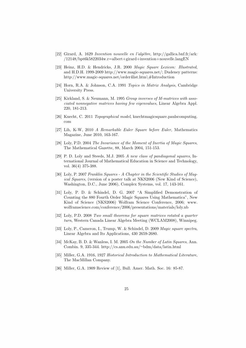
Figure 1: Entropy as a function of order n for MATLAB routine magic(n).

• Compound magic squares (CMSs) [47] of order n = pq have order p or qtiled magic subsquares. These begin at n = 9 and are interesting becausethey have lower ranks than all but Franklin type magic squares when theyshare the same doubly even order (n = 12, 16, 20, 24, ...).

5.2 Overview of magic squares as order increases

Figure 1 shows the results of using the MATLAB magic(n) function (we usemagicn to identify these in later tables), together with the upper bound of ln(n)for n = 3...100. MATLAB [37] uses one algorithm to produce non-singular(full rank) associative magic squares for odd order, and a second algorithmfor singular even order magic squares which are not associative but have rank(n+ 4) /2. MATLAB’s third algorithm gives a family of rank 3 (singular) doublyeven magic squares.

Figure 1, while based on the MATLAB algorithms, suggests that higher rankmagic squares have the higher entropies, with rank three magic squares havingthe lower entropies. This figure is analogous to one presented in Rao et al [46]in the context of the Indus script.

5.2.1 Large n limit for doubly even cases

Kirkland and Neumann [25] showed that MATLAB’s third algorithm leads toalgebraic results for the three non-zero eigenvalues and SVs. As n → ∞, theratio σ1/σ2 →

√3, while σ3/σ1 → 0, with the result that H → 0.6568..., in

8

+

+

+

+

+

+

+

+

+

+

+

++

++

+++

+

+

++

+

+

+

+

++

+

+

+++

+

+

+

+

+

+

+

+

+

+++++

++

+

+

++

+

+

++

+

+

+

+

++

+

+ ++

+

+

++

++

+

+

+

+

+

+

+

+

++

+

+

+

+

+

++

+

+

+

+

+

+

+

+

+

++

+

+

++

++

+

+++

++

++

++

+

++

+

+ +

+

+

++

+

+

+

+

+

+

+

+

+

+

+

+

+

+

+

+

+

+

+

+

+

+

+

+++

+

+

+

+

+

+

+

+

+

+

+

+

++

+

+

+

+

+

+

+

++++

+

+

+

+

+

+

+

+

+

+

+

+

++

+

+

++

+

+

+

+

+

+

++

+

+

+

+

+

+

+

+

++

+

+

+

+++

+++

+++

+

++

+

+

+

++

+

+

+

+

+

+

+

+

+

+

+++

+

+

+

+

+++

++

+

+

+

+

+

+

+

++

+

+

+

++

+ +

+

+

+

+

+

+

+

+

+

+

+

+

+

+

++

++

++

+

+

+

++

+

+

+

++

+

++

+

+

+

+

+

+

+

+

+

+

+++

+

+

+

+

++

+

+

+

+

+

+

+

+

+

+

+

+

+

+

+

+

+

+

+

+

+

+

+

+

+

+

+

++

+

+

+

+

+

+

+++

+

+

+

+

+

+

+

+

+

+

+

+

+

+

+

+

+

+

+

+

+

+

++

+

+

+

+

+

++

+

++

+

+

++++

+

+

+

+

+

+

+

+

+

+

+

+

+

+

+

+

+

+

++

+

+++

++

++

+

+

+

+

++

+

+

+

+

+

+

+

+

++

+

+

+

+

+

+

+

+

+

+

+

+

+

+

+

+

+++

+

+

++

+

++

+

+

+

+

+

++

+

+

+

+

+

+

+

++

+

+

+

+

+

+

+

+

+

++

++

+

++

++

+

+

++

++

+

+

+

+

++

+

+

+

+

+

+

+ +

+

+

+

+

+

+

+

+

+

++

++

+

++

+

+

+

+

+

+

+

+

++

+

+

+

++

+

+

+

+

+

+

+

+ +

+

+

++

+

+

+

+

+

+++

+

+

+

+

++

+

+

+

+

+

+

++

+++

++

+

+

+

+

+

++

+

+

+

+

+

+

+

+

+

++

+

+

+

+

++ +

++

+

++

++

+

+

+

+

+

++

+

+

+

+ ++

+

++

++

+

+

+

+

+

+

+

+

++

+

+

+++

+

++

+

+

++ ++

+

+

++

+

+++

+

+

+

+

++

+

+

+

+

++

++

+

+

+

+

+

+

+

+

+

+

+

+++

+

+

+

+

+

+

+

+ +

+

++

+

+

+

+

+

+

+

+

+

+

++

+

+

++

+

+

+

++

+

++

++

+

+

+

+

++

+

++

++

+++

+

+

+

+

+

+

+

+

+

+ +

+

+

+

+

+

+

+

+

+

+

+

+

+

+

++

+

+

++

++ +

+

+

+

+

+

+

+

+

+

+

+

+

+

+

+++

+

+

+

+

++

+

+

+

+

+

+

+

+

+

+

+

+

+

+

+

+

+

++

++

+

+

+

+

+

+

+

+

+

+

+

+

+

++

+++

++

+

+

+

+

+

+

+

++

++

+

+ +

+

+

+

+

+

+

+

+

2 4 6 8 10 12

0.80

0.85

0.90

0.95

1.00

1.05

1.10

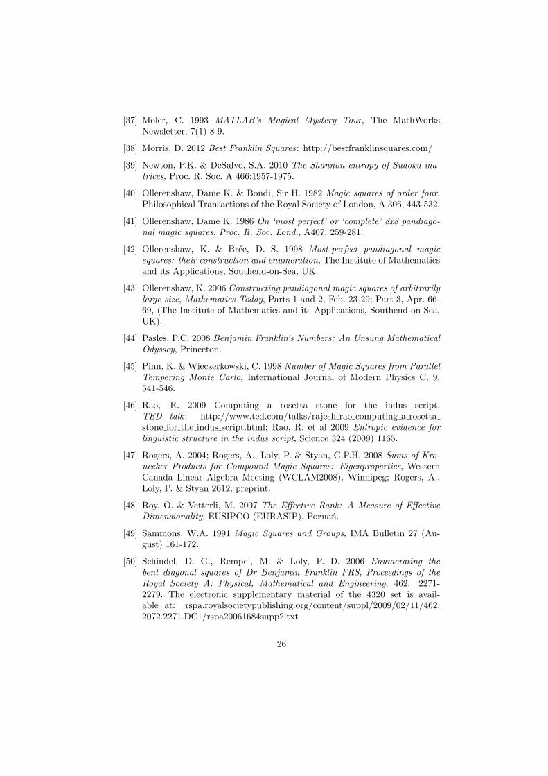
Figure 2: H-values for Dudeney’s groups

accord with the asymptotic lower branch of Figure 1. The compression (7)

increases gradually with n as(1− H

ln(n)

), becoming 95.25% for n = 106. Also,

index R can be exactly calculated from their SV formula since their squares areintegers.

5.3 Complete set of order 4 magic squares

Dudeney [14] gave the first complete classification of Frenicle’s [3] 880 magicsquares into a dozen Groups, I-XII, distinguishing arrangements in order fourmagic squares made by linking pairs of elements which sum to 17 = 1+(n = 4)

2.

Group VI splits into two distinct sets of SV values, the semi-pandiagonal setVI-P sharing SVs with Groups IV and V, and VI-S with quite distinct SVs,justifying the split made by Dudeney.

For this set Loly, Cameron, Trump and Schindel [33] used values of σ22 to

find 63 distinct SVs, however the NDS work was not available to suggest anyfurther exploration at that time. Now it is clear that there are five Supergroups;A, with Groups I (pandiagonal), II (semi-pandiagonal and semi-bent), and III(associative); B, with Groups IV, V, and V-P which are all semi-pandiagonal;C, with just Group VI-S which stands alone (and which Dudeney [14] haddistinguished from Group VI-P); D, with Groups VII, VIII, IX and X and finallyE, with Groups XI and XII. The 640 members of Groups I-VI are singular withrank 3, while the 240 members of Groups VII-XII are non-singular with rank 4.For numerical convenience in sorting and plotting results we list the DudeneyGroups by a numerical label 1− 12, with the subgroup VI-S as 6.5, since it fitslogically between Groups VI-P and VII.

Figure 2 shows the Shannon entropy H versus these numerical group labelsin order to emphasize the Supergroup sets, and so that the high and low valuesof the entropies of the Supergroups can be compared.

In Table 1 we examine entropies of this set for representative individual

9

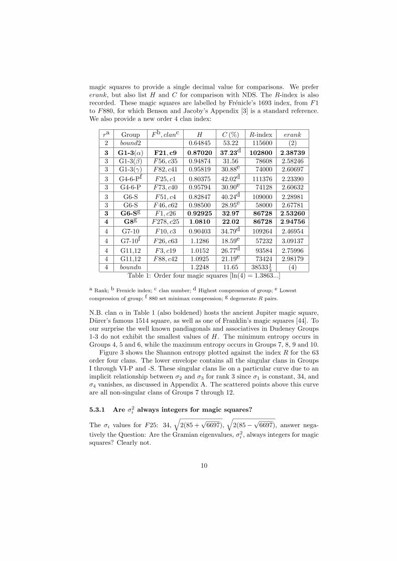
magic squares to provide a single decimal value for comparisons. We prefererank, but also list H and C for comparison with NDS. The R-index is alsorecorded. These magic squares are labelled by Frenicle’s 1693 index, from F1to F880, for which Benson and Jacoby’s Appendix [3] is a standard reference.We also provide a new order 4 clan index:

ra Group Fb, clanc H C (%) R-index erank2 bound2 0.64845 53.22 115600 (2)

3 G1-3(α) F21, c9 0.87020 37.23d 102800 2.387393 G1-3(β) F56, c35 0.94874 31.56 78608 2.582463 G1-3(γ) F82, c41 0.95819 30.88e 74000 2.60697

3 G4-6-Pf F25, c1 0.80375 42.02d 111376 2.233903 G4-6-P F73, c40 0.95794 30.90e 74128 2.60632

3 G6-S F51, c4 0.82847 40.24d 109000 2.289813 G6-S F46, c62 0.98500 28.95e 58000 2.677813 G6-Sg F1, c26 0.92925 32.97 86728 2.532604 G8g F278, c25 1.0810 22.02 86728 2.94756

4 G7-10 F10, c3 0.90403 34.79d 109264 2.46954

4 G7-10f F26, c63 1.1286 18.59e 57232 3.09137

4 G11,12 F3, c19 1.0152 26.77d 93584 2.759964 G11,12 F88, c42 1.0925 21.19e 73424 2.981794 boundn 1.2248 11.65 38533 1

3 (4)Table 1: Order four magic squares [ln(4) = 1.3863...]

a Rank; b Frenicle index; c clan number; d Highest compression of group; e Lowest

compression of group; f 880 set minimax compression; g degenerate R pairs.

N.B. clan α in Table 1 (also boldened) hosts the ancient Jupiter magic square,Durer’s famous 1514 square, as well as one of Franklin’s magic squares [44]. Toour surprise the well known pandiagonals and associatives in Dudeney Groups1-3 do not exhibit the smallest values of H. The minimum entropy occurs inGroups 4, 5 and 6, while the maximum entropy occurs in Groups 7, 8, 9 and 10.

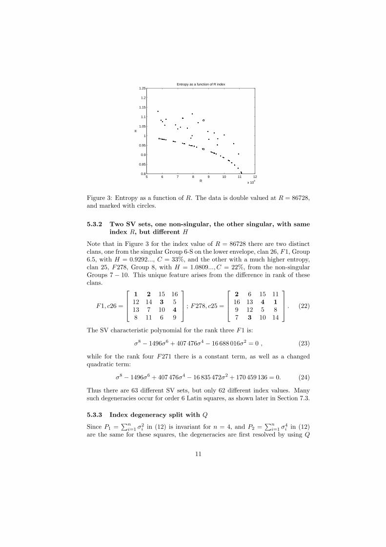
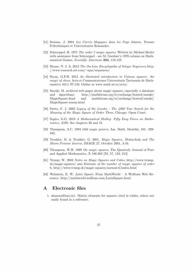
Figure 3 shows the Shannon entropy plotted against the index R for the 63order four clans. The lower envelope contains all the singular clans in GroupsI through VI-P and -S. These singular clans lie on a particular curve due to animplicit relationship between σ2 and σ3 for rank 3 since σ1 is constant, 34, andσ4 vanishes, as discussed in Appendix A. The scattered points above this curveare all non-singular clans of Groups 7 through 12.

5.3.1 Are σ2i always integers for magic squares?

The σi values for F25: 34,√2(85 +

√6697),

√2(85−

√6697), answer nega-

tively the Question: Are the Gramian eigenvalues, σ2i , always integers for magic

squares? Clearly not.

10

5 6 7 8 9 10 11 12

x 104

0.8

0.85

0.9

0.95

1

1.05

1.1

1.15

1.2

1.25

R

H

Entropy as a function of R index

Figure 3: Entropy as a function of R. The data is double valued at R = 86728,and marked with circles.

5.3.2 Two SV sets, one non-singular, the other singular, with sameindex R, but different H

Note that in Figure 3 for the index value of R = 86728 there are two distinctclans, one from the singular Group 6-S on the lower envelope, clan 26, F1, Group6.5, with H = 0.9292..., C = 33%, and the other with a much higher entropy,clan 25, F278, Group 8, with H = 1.0809..., C = 22%, from the non-singularGroups 7 − 10. This unique feature arises from the difference in rank of theseclans.

F1, c26 =

1 2 15 1612 14 3 513 7 10 48 11 6 9

; F278, c25 =

2 6 15 1116 13 4 19 12 5 87 3 10 14

. (22)

The SV characteristic polynomial for the rank three F1 is:

σ8 − 1496σ6 + 407 476σ4 − 16 688 016σ2 = 0 , (23)

while for the rank four F271 there is a constant term, as well as a changedquadratic term:

σ8 − 1496σ6 + 407 476σ4 − 16 835 472σ2 + 170 459 136 = 0. (24)

Thus there are 63 different SV sets, but only 62 different index values. Manysuch degeneracies occur for order 6 Latin squares, as shown later in Section 7.3.

5.3.3 Index degeneracy split with Q

Since P1 =∑n

i=1 σ2i in (12) is invariant for n = 4, and P2 =

∑ni=1 σ

4i in (12)

are the same for these squares, the degeneracies are first resolved by using Q

11

in (17). In this case, since b1 and b2 are the same, this is due entirely to thedifferent b3’s, for an amount 442368 (for both L,R).

5.4 Complete Set of order 5 Magic Squares

A similar analysis has been carried out for the 275, 305, 224 order 5 magic squareswhere there is no comparable classification scheme so that the distribution ofH and C obtained gives new insight into that large complete set. There areno rank 3 fifth order magic squares, only the singular rank fours and full rankfives. A few examples are given in Table 2, together with the bounds outlinedin section 4.2.

Eight clan pairs of ultramagic squares [55] are included in Table 2. To saveon display space the matrix elements are relegated to the Electronic Supplement,shannonData.txt.

r square H C (%) R erank4 bound2 0.91420 43.2 1, 690, 000 (2)4 lcts43m2a 1.05067 34.72 1, 218, 640 2.85955

5 suz6, 9b 1.12526 30.08 954, 480 3.08101

5 suz2, 13b 1.12706 29.97 904, 500 3.086584 lcts44m4a 1.20122 25.36 706, 000 3.32418

5 suz5, 10b 1.20354 25.22 822, 000 3.33188

5 lcts45a, suz1, 14b 1.23161 23.48 772, 980 3.426744, 5 full set 1.2827 20.3

5 suz7, 12b 1.37667 14.46 522, 480 3.96171

5 suz3, 16b 1.3783 14.36 544, 500 3.96813

5 suz8, 11b 1.38085 14.20 582, 000 3.97827

5 suz4, 15b 1.38229 14.11 604, 980 3.984035 magic5c(Mars) 1.38932 13.68 532, 000 4.012125 boundn 1.442 10.4 422, 500 (5)

Table 2: n = 5 [entropy increases down column 5, ln (5) = 1.6094...]

a[33]; b[55]; c[37].

The maximum range of R values in Table 2 is only 1 690 000 − 422 500 =1 267 500, and this must accommodate 275, 305, 224 squares with 22, 598, 324different clans, so while R might still be useful as a preliminary index for or-der five, further index splitting with Q in (17) is eventually needed because ofinevitable degeneracies in R. Also the ratio of extreme compressions for orderfive is about 4 : 1, compared to 2.25 : 1 for the order fours, but well within the5 : 1 of the order five bounds.

For the higher compression suz6, 9 the respective contributions of the de-scending SVs to the entropy are: {0.3308, 0.3468, 0.2989, 0.08561, 0.0632}, whereas usual σ2 is the largest contribution, and the last two are much smaller thanfirst three. The lower compression suz4, 15 exhibits an effect not so far found in

12

our studies of any other magic squares, namely the first SV, σ1, gives the largestcontribution to the entropy: {0.3507, 0.3195, 0.2563, 0.2323, 0.2234}, with thelast three SVs all substantial.

Walter Trump (2007) Trump [61] found the eigenvalue characteristic poly-nomials of 245, 824 different singular cases, which is less than 0.1% of 275, 305, 224squares. He also found 10 different determinants for the non-singular cases.

6 Higher orders

The situation for higher orders is more difficult because there are only statisticalestimates of the very large populations for order six and higher [45, 61]. We skipto order 8 and 9 for which there are many interesting cases. For order 8 someexamples closely approach the bounds outlined in section 4.2, especially for thelower entropy bound of order 8. Our data for orders 6 and 7 fall well short ofthe lower entropy bounds and in neither case do we have a rank three example.Order 9 affords a link to NDS which prompted the present work. Euler [17] hadshown how Latin squares could be used to construct some natural magic andsemimagic squares.

6.1 Order 8 magic squares

Trump [61] estimated that there are about 5.2 × 1054 magic squares for ordereight, while we have a range of R about 409 × 106 from the bounds in Table3. Amongst other data which we are able to include at order 8 is the completeset of Ben Franklin’s 8th order squares constructed by Schindel, Rempel andLoly [50]. That study did not examine their eigenproperties, but subsequentlythey were all found to have rank 3. These Franklin squares exhibit 64 clans. InTable 3, we show several order 8 magic squares with rank 3, the minimum rankfor magic squares (Drury [13]) [see Appendix A for simplifications for rank 3,which we discussed earlier for order four].

13

r square H C (%) R erank2 bound2 0.65479 68.51 476, 985, 600 (2)

3 bf min a,b 0.70720 65.99 476, 125, 440 2.02830

3 magic8c 0.80335 61.37 462,534,912 2.23301

3 dko86d 0.87072 58.13 431, 200, 512 2.388624 wht8ae 0.91569 55.96 431, 560, 960 2.498503 bf max a 0.97144 53.28 299, 964.672 2.64173

7 gaspalou13f 1.2867 38.12 224, 354, 880 3.62073

5 euler8g,b 1.4157 31.92 136, 171, 776 4.11942

7 bimagich (bi8a) 1.5251 26.66 152, 375, 424 4.59565

8 i88e8i 1.5480 25.56 283, 664, 192 4.70214

7 wtREG841BIj 1.6829 19.07 102, 971, 488 5.38120

8 eulerKnightk,b 1.6887 18.79 146, 064, 640 5.412338 boundn 1.8415 11.44 68, 140, 800 (8)

Table 3: n = 8, [ln (8) = 2.0794...]

a Franklin 4320 set [50] bf min(H), [max (C)]; b semimagic; c [37] and many other squares;d

[41]; e [60]; f [21]; g [17]; h[5]; iIan8 [lowest H]; j[61]; k[17].

The most highly compressed clan, (Franklin) bf min, is shown at the topof Table 3 (C = 66%, which is 96% of our upper bound compression) followedclosely by the magic8 MATLAB square. These are displayed below:

bf min =

1 63 8 58 3 61 6 6056 10 49 15 54 12 51 1357 7 64 2 59 5 62 416 50 9 55 14 52 11 5317 47 24 42 19 45 22 4440 26 33 31 38 28 35 2941 23 48 18 43 21 46 2032 34 25 39 30 36 27 37

, magic8 =

64 2 3 61 60 6 7 579 55 54 12 13 51 50 1617 47 46 20 21 43 42 2440 26 27 37 36 30 31 3332 34 35 29 28 38 39 2541 23 22 44 45 19 18 4849 15 14 52 53 11 10 568 58 59 5 4 62 63 1

.

(25)The recurrent MATLAB magic8 clan (boldened in Table 3) is also shared

by many other squares: the ancient Mercury square, laa(42)[33], i8, as wellas #1127 of the 4320 set of Franklin squares [50]. LCTS [33] found the SVsfor MATLAB magic8 to be σi = {260, 32

√21, 4

√21}, with five zeroes (rank

3). We now find that his clan has R = 462, 534, 912, and is shared with one ofthe 10 pandiagonal Franklin clans (64 in total), with effective rank 2.233. Wesuggest that these are all related by SV conserving transforms of one another.

It may be worth noting the SVs of a few of the simpler clans: bf min:

σi = {260, 2√2(1365 +

√1856505), 16

√210/(1365 +

√1856505)}, and bf max:

σi = {260, 28√21, 16

√21}. Clearly these order 8 rank three magic squares have

low entropy. ”Franklin” type squares of doubly even order with rank three areknown to n = 48 [38], and they have progressively lower entropy.

George Styan Of special interest in connection with our celebration of GeorgeStyan’s 75th, we examine a set of magic squares with knight’s paths, especially

14

a type called Caıssan [54]. We note that the magic8 clan is also shared byhis Caıssan ”beauty” square, caiss8Q4, as well as his ursus and bcm3. EarlierBeverly (1848) [59] gave a semi-magic knight tour square bev8, which we nowfind has the same clan as euler8 in Table 3.

Applying our methods to the Caıssan squares reveals that they have the samesignatura as the Franklin pandiagonal squares and the 8th order most perfectsquares of Ollerenshaw, indicating that these groups are related if indeed notthe same.

Another interesting feature which Styan studies concerns knight-Nasik or-der 8 pandiagonal magic squares and the geometric patterns formed by linesdrawn through successive elements connected by moves of a chess knight (Styan’sCSP2,3). Related line patterns are quite old [6, 59].

6.2 Order 9

To afford a closer comparison with the order 9 study of NDS, we have includeda few sample magic squares for order 9 in Table 4.

r square H C (%) R erank2 bound2 0.65522 70.18 1, 960, 718, 400 (2)5 ta, tda 1.12999 48.57 1, 301, 165, 856 3.09562

9 txb 1.20501 45.16 1, 307, 982, 296 3.336795 dko9ac 1.33486 39.25 788, 778, 000 3.79948

9 bimagic9d 1.55931 29.03 783, 193, 032 4.755537 dko9bc 1.69577 22.82 413, 322, 912 5.450829 lunae 1.85005 15.80 472, 695, 264 6.36014

9 magic9f 1.85479 15.69 455, 689, 152 6.375609 boundn 1.9490 11.30 245, 089, 800 (9)

Table 4: n = 9 [ln (9) = 2.1972...]

a ta, td [51]; b tx [16]; c dko9a, b [43]; d bimagic9 [5]; e luna (magic square of the Moon); f

magic9 [37].

Comparison of rank 9 tx with rank 5 ta shows that SVs of the latter decreasefaster for a slightly smaller R:

tx: {369, 187.213, 94.4392, 11.0905, 9.8952, 6.9375, 5.7113, 3.2663, 0.47874}.ta: {369, 187.061, 93.5307, 20.7846, 10.3923, 0, 0, 0, 0}.Pfefferman’s bimagic9 of 1891 [43] has a degenerate pair (boldened), a much

smaller R-index and higher entropy than tx which has the same full rank:bimagic9: {369,140.296,140.296, 46.765, 42.042, 24.823, 15.589, 8.559, 5.196}Compound magic squares (CMSs) of order n = pq; p, q ≥ 3, which begin

at order 9, have the same 3-partitioned substructure as the Sudokus studied byNDS, albeit now with distinct sequential matrix elements, e.g. for n = 9 withelements 1...81. Rogers, Loly and Styan [47] have shown that order 9 CMSsare highly singular with rank 5 at order 9, whereas NDS found only Sudokuswith ranks 8 and 9. The CMSs ta, and a permuted partner td, date respectively

15

from 983 CE and 1275 CE. They share the same eigenvalues and singular values.For comparison observe that van den Essen’s X-sudoku magic square [16], tx,has the same numbers in each subsquare as does ta, but without the magicsubsquares which are increments of the Loshu:

ta =

71 64 69 8 1 6 53 46 5166 68 70 3 5 7 48 50 5267 72 65 4 9 2 49 54 4726 19 24 44 37 42 62 55 6021 23 25 39 41 43 57 59 6122 27 20 40 45 38 58 63 5635 28 33 80 73 78 17 10 1530 32 34 75 77 79 12 14 1631 36 29 76 81 74 13 18 11

, tx =

68 72 70 6 4 3 47 46 5365 67 66 1 8 7 54 51 5071 69 64 2 9 5 49 52 4821 26 23 43 37 45 60 56 5827 20 24 44 39 40 61 59 5519 25 22 41 38 42 57 62 6333 30 29 81 77 73 17 13 1631 28 35 75 79 74 14 18 1534 32 36 76 78 80 10 12 11

.

(26)Ollerenshaw’s 2006 rank 5 square [43] dko9a was constructed from a magic

Sudoku square, and while 3-partitioned, is not a CMS since the subsquares arenot magic, though their elements do sum to nine times the magic sum (369).

7 Latin squares and Sudoku solutions

Now we look at the Latin squares for the insight that these simpler objectsgive into magic squares, including the R-degeneracy already found for order4 magic squares, the connection to NDS, and knowing that Euler [17] showedthat some magical squares can be constructed from them. Numerical (integer)Latin squares (elements 1...n repeated n times with each once in every row andcolumn) have the same line sum of elements in all Rows and Columns (RCsquares) but not necessarily for the diagonals (D1 and D2), specifically:

Latin line sum: sn = (1 + 2 + ...+ n) = n (1 + n) /2; n > 1. (27)

Some Latin squares are RCD, but with repeated elements. Ninth order Sudokushave the additional constraint that each integer appears only once in each ofthe nine adjoining 3×3 subsquares, also called 3-partitioned [15]. Latin squaresmay be classified in several ways, e.g. Weisstein [62] gives 12 for order 3, beforenoting that there is just one normalized square with the first row and columngiven by {1, 2, ..., n} at this order. Our focus on distinct SV sets uses thesenormalized Latin squares.

The smallest Latin square, lat2, is bisymmetric, has λi = {3,−1}, σi ={3, 1}, D1 = 2 = D2 = 4. Then L = 82, R = 1, H = 0.562..., erank = 1.755...,C = 19%:

lat2 =

[1 22 1

]; lat3 =

1 2 32 3 13 1 2

(28)

The sole order three lat3 is shown above and has σ1 = {6,√3,

√3}, H =

0.9105..., C = 17%, erank = 2.4856..., L = 1314 and R = 18.

7.1 Order 4 Latin squares have 4 clans

Here there are 4 normalized reduced Latin squares [62] which show some differ-ences in their spectral properties, especially the SVs. lat4a is a bisymmetric case

16

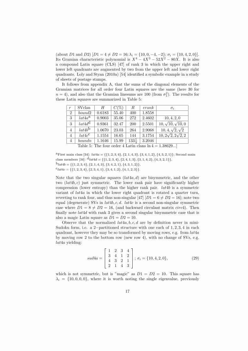
(about D1 and D2) [D1 = 4 = D2 = 16;λi = {10, 0,−4,−2}; σi = {10, 4, 2, 0}].Its Gramian characteristic polynomial is X4 − 4X3 − 52X2 − 80X. It is alsoa compound Latin square (CLS) [47] of rank 3 in which the upper right andlower left quadrants are augmented by two from the upper left and lower rightquadrants. Loly and Styan (2010a) [54] identified a symbolic example in a studyof sheets of postage stamps.

It follows from appendix A, that the sums of the diagonal elements of theGramian matrices for all order four Latin squares are the same (here 30 forn = 4), and also that the Gramian linesums are 100 (from σ2

1). The results forthese Latin squares are summarized in Table 5:

r SVclan H C(%) R erank σi

2 bound2 0.6183 55.40 400 1.85583 lat4aa 0.9003 35.06 272 2.4602 10, 4, 2, 0

3 lat4dd 0.9361 32.47 200 2.5501 10,√10,

√10, 0

4 lat4bb 1.0670 23.03 264 2.9068 10, 4,√2,√2

4 lat4cc 1.1554 16.65 144 3.1754 10, 2√2, 2

√2, 2

4 boundn 1.1646 15.99 133 13 3.2046

Table 5: The four order 4 Latin clans ln 4 = 1.38629...]

aFirst main class [34]: lat4a = {{1, 2, 3, 4}, {2, 1, 4, 3}, {3, 4, 1, 2}, {4, 3, 2, 1}}; Second main

class members [34]: dlat4d = {{1, 2, 3, 4}, {2, 4, 1, 3}, {3, 1, 4, 2}, {4, 3, 2, 1}},blat4b = {{1, 2, 3, 4}, {2, 1, 4, 3}, {3, 4, 2, 1}, {4, 3, 1, 2}},clat4c = {{1, 2, 3, 4}, {2, 3, 4, 1}, {3, 4, 1, 2}, {4, 1, 2, 3}}.

Note that the two singular squares (lat4a, d) are bisymmetric, and the othertwo (lat4b, c) just symmetric. The lower rank pair have significantly highercompression (lower entropy) than the higher rank pair. lat4b is a symmetricvariant of lat4a in which the lower right quadrant is rotated a quarter turn,reverting to rank four, and thus non-singular [47] [D1 = 6 = D2 = 16]; note twoequal (degenerate) SVs in lat4b, c, d. lat4c is a second non-singular symmetriccase where D1 = 8 = D2 = 16, (and backward circulant matrix circ4). Thenfinally note lat4d with rank 3 gives a second singular bisymmetric case that isalso a magic Latin square as D1 = D2 = 10.

Observe that the normalized lat4a, b, c, d are by definition never in mini-Sudoku form, i.e. a 2−partitioned structure with one each of 1, 2, 3, 4 in eachquadrant, however they may be so transformed by moving rows, e.g. from lat4aby moving row 2 to the bottom row (new row 4), with no change of SVs, e.g.lat4a yielding:

sud4a =

1 2 3 43 4 1 24 3 2 12 1 4 3

; σi = {10, 4, 2, 0}, (29)

which is not symmetric, but is ”magic” as D1 = D2 = 10. This square hasλi = {10, 0, 0, 0}, where it is worth noting the single eigenvalue, previously

17

observed for some order 4 natural magic squares by Loly et al [33]. The lat4b, csquares transform into mini-Sudokus by the same row changes as above, whilelat4d transforms to sud4d by moving row 4 to become the new row 2. In allthese cases the SVs are unchanged, and so H, C, L, R and erank are alsounchanged.

The entries in Table 5 were ordered according to increasing H (and erank,but decreasing C), while R shows some deviation (seen also in some of ourlater tables). Since all measures depend on the SVs, the different (descending)magnitudes of these are responsible for any variations, e.g. only lat4c has thelargest contribution to H from the leading SV, σ1, while the others have theirlargest contribution from σ2 (and for the degenerate σ2 = σ3 for lat4d).

7.2 Order 5 Latins have 7 clans

For this prime order the 56 normalized Latin squares (Weisstein 2011) [62] allhave rank 5, i.e. non-singular, having only seven clans (different entropies,compressions, effective ranks, etc.), as reported in Table 6 with the number ofnormalized squares in each clan in brackets (from 1 to 20), each with a distinctR index in order of the descending compressions, and all within the bounds of625 (just) to 2500. None are magic in standard form.

square H C(%) R erankbound2 0.6272 61.03 2500 1.8723

lat5f(1)a 1.0911 32.20 1230 2.9776

lat5b(20)b 1.1741 27.05 1038 3.2351lat5e(2)a 1.2618 21.60 1030 3.5319

lat5a(20)b 1.2973 19.39 978 3.6594

lat5d(10)b 1.3259 17.62 798 3.7654lat5c(1)a 1.3421 16.61 750 3.8272lat5g(2)a 1.3646 15.21 630 3.9142boundn 1.3655 15.16 625 3.9175

Table 6: The seven order 5 Latin clans - all rank 5 [ln (5) = 1.6094...]

a First main class [34]; b 2nd main class [34].

Again the maximum compression, C = 32.20...%, of this set falls well short ofthe upper bound, C = 61.03...%. Note also that the surd-in-surd structure of

the σ2...4 for lat5f , namely√(25± 11

√5)/2 (twice), shows that not all Latin

squares have integer σ2i , as did n = 4 Latins. Also lat5b...g in Table 3 have the

largest contribution to H from the leading SV, σ1, while lat5f has two equalcontributions from its degenerate σ2 = σ3, with almost as much from σ1.

7.3 Order 6 Latins have 599 clans

Of the 9408 normalized squares [34, 57] (none magic), we find 158 of rank 4 in22 clans with 20 R-indices; 1568 of rank 5 in 91 clans with 73 keys (R-indices);

18

and 7682 of full rank in 486 clans with 282 keys (R-indices). Two pairs of rank 4squares have R-indices 5409 and 4689 respectively, but distinct entropies. Thereare multiple clans with the same R-index but distinct entropies in the range ofR : 2229...6849, within the bounds 2205 (just) to 11, 025. Clearly order six Latinsquares are more complicated than the preceding orders.

We show just the pair of compound Latin squares [47] for order 6 and rank4, which are formed from the two combinations of lat2 and lat3, the first 2-ply,the second 3-ply [15]:

cls6a =

1 2 3 4 5 62 3 1 5 6 43 1 2 6 4 54 5 6 1 2 35 6 4 2 3 16 4 5 3 1 2

, cls6b =

1 2 3 4 5 62 1 4 3 6 53 4 5 6 1 24 3 6 5 2 15 6 1 2 3 46 5 2 1 4 3

. (30)

Their properties are listed in Table 7, along with a selection of other examples.Note that there are also corresponding order six Sudokus with respectively 2×3and 3× 2 blocks with the same SVs and other Shannon properties as cls6a andcls6b respectively.

r square H C(%) R erank2 bound2 0.6327 64.69 11025 1.88274 pair1a 1.0575 40.98 5409 2.87924 pair2 1.0942 38.93 5409 2.9868

4 cls6ab, sud6a, bailey4 1.1090 38.10 6849 3.03154 cls6bc, sud6b, quartet1 1.1494 35.85 4689 3.15624 quartet2 1.1660 34.92 4689 3.20915 quartet3 1.1773 34.29 4689 3.24565 sextet1 1.3445 24.96 3537 3.83636 quartet4 1.3621 23.98 4689 3.90446 sextet2 1.3699 23.54 3537 3.93506 sextet3 1.4067 21.49 3537 4.08256 sextet4 1.4271 20.35 3537 4.16666 sextet5 1.4298 20.20 3537 4.17796 sextet6 1.4302 20.18 3537 4.1795

6 costas6d, circ6, albuni6 1.4920 16.73 2961 4.44616 singleta 1.5308 14.56 2229 4.62196 boundn 1.5320 14.50 2205 4.6273

Table 7: Selected order 6 Latin clans [ln (6) = 1.7918...]

aset limits; b σi = {21, 4√3, 4

√3, 3, 0, 0}; c σi = {21, 9, 2

√3, 2

√3, 0, 0};d

σi = {21, 6, 6, 2√3, 2

√3, 3}.

Note the degenerate SVs for clsa, b and costas6. Table 7 includes a quartetwith R = 4689, a sextet with R = 3537, a square for a Costas array [12]

19

with the same clan as an order six circulant, circ6, and a remarkable XII-XIIIcentury square from Al-Buni (Descombes 2000) [11] in the Arabic symbols for1, 2, 4, 6, 8, 9 which we relabelled to 1...6, denoted by albuni6 some time beforeEuler.

7.4 Order 9 Latin squares and low rank order 9 Sudokus

There are 377, 597, 570, 964, 258, 816 normalized Latin squares [62]. NDS sus-pected that there were no Sudokus with algebraic multiplicity more than 1, i.e.just rank 8 and 9, but were not able to prove that. We have now been able togenerate Sudokus of ranks 5, 6 and 7 as well as a few others with ranks 8 and9, and include their properties in Table 8.

r square H C (%) R erank2 bound2 0.6414 70.81 291, 600 2.899139 idc15m 1.2288 44.08 142, 236 3.417125 cls9, idc5pa 1.2952 41.05 119,556 3.651826 idc6p 1.4296 34.94 100, 692 4.177107 idc7p 1.5389 29.96 94, 644 4.659259 knecht 1.5610 28.96 101, 028 4. 763398 idc8p 1.6406 25.33 82, 752 5.158149 bailey12 1.6700 23.99 76, 208 5.31231

8 nds21b 1.7119 22.09 66, 864 5.539229 idc9pc 1.7127 22.05 76, 936 5. 543639 bailey11 1.7610 19.85 62, 636 5.818519 ndsfig1 1.7789 19.04 63, 408 5.923359 nds22 1.8163 17.34 67, 068 6.14895

9 idc69d 1.8878 14.05 40, 824 6.605069 albuni9 1.9080 13.16 36, 972 6.739809 idc14me 1.9083 13.15 36, 936 6.741679 boundn 1.9099 13.08 36, 450 7.75220

Table 8: Order 9 Latins and Sudokus from rank 5 to rank 9.

aσi = {45, 9√3, 9

√3, 3

√3, 3

√3, 0, 0, 0, 0};

bσi = {45, 13.968, 10.672, 9.337, 9.041, 5.628, 4.6463, 2.971, 0};cσi = {45, 14.953, 11.180, 8.644, 8.337, 4.973, 4.033, 2.331, 0.874};dσi = {45, 9, 9, 9, 9, 9, 9, 3

√3, 3

√3}; eσi = {45, 9, 9, 3

√7, 3

√7, 3

√7, 3

√7, 3

√7, 3

√7}.

In Table 8 there is a CLS iterated from lat3 with 3× 3-ply, cls9, which has thesame clan properties as idc5p in Table 9 above. It can also be transformed toSudoku form by row and column permutations. Since these matrices take a lotof display space, their matrix elements are listed in an Electronic Supplement,shannonData.txt. We found that the clan represented by cls9, idc5p (boldened)has recurred frequently, probably because of ease of construction. These mustbe clan members related by transformations which preserveH and these serve toillustrate the usefulness of our clan concept in identifying related squares. While

20

we initially found that lower rank Sudokus had lower entropy, further examplesof full rank but lower entropy prompted the introduction of the effective rankmeasure. This is dramatically illustrated by the top entry in Table 8 wherewe found a full rank Sudoku with C = 44% compression. Another full rankSudoku, knecht, provided by Craig Knecht [26] also has low effective rank butwas constructed by criteria involving water retention in 3D models of Sudokus.Note that cls9 and idc5p, with high compression, and idc69 and idc14m, withvery low compressions, each have rather pretty SVs in surd form. As well almostthe smallest compression found so far is for a remarkable Arabic Latin squareof Al-Buni from the XII-XIII century [11], albuni9, which has properties veryclose to idc14m in Table 9. We now know from a suggestion by Lih [27] thatthat a Korean magic square constructed by Choe (1646–1715) from a pair ofLatin squares, choeL and choeR, shares the same clan as the recurring idc5p.

8 Summary

While the key issue is the usefulness of isentropic clans, we found that theeffective rank measure erank is a better guide for comparing different orders ofboth magic and Latin squares than the entropies, which have an upper boundof ln(n). As this work progressed, an early view that the low entropy of magicalsquares was associated with low rank was dispelled by finding some full rankexamples with very low entropy. Very high compressions and low effective rankswere found for doubly even magic squares which often exhibit rank 3, as wellas for compound magic squares which also exhibit much less than full rank.Aside from a pair of order four magic clans (see 22), order six Latin squaresgive examples of different clans with duplicate R indices.

Our link to Girard’s work [35] followed from a critical review of Andrews’book [1] by G.A. Miller [36]. As the magnitudes of the indices R and Q growwith increasing order n, it would eventually be necessary to use higher precisionarithmetic to clarify differences in H, C and erank. These various measuresconstitute our signatura.

Contrasting our new results with those of NDS’s order nine rank 8 and 9Latin and Sudoku random ensembles suggests that our lower rank examplesare relatively rare and so less likely to be found in those ensembles, but theirapparent ease of construction means that these often recur historically. Studyingwhether there is any correlation between the difficulty of Sudoku puzzles andthe measures introduced here might make an interesting student project.

We have shown that the clan concept is useful in classifying historical magicalsquares, as well as new examples as they are generated. We propose a “Libraryof Magical Squares”, where R is used to find the correct shelf, and Q the properposition on that shelf.

The use of eigenvalue and singular value considerations in this work shouldnot be a deterrent to wider use of the measures advocated here. For advice inimplementing these ideas contact Ian.Cameron@ad.umanitoba.ca for FreeMat,Macsyma, Python, Octave; rogers@physics.umanitoba.ca for MATLAB and

21

Maple; or loly@cc.umanitoba.ca for Mathematica, Maple, Wolfram Alpha viaweb browser and iPad.

9 Acknowledgements

We thank Wayne Chan, Daniel Schindel, George Styan, Harvey Heinz, Wal-ter Trump, Francis Gaspalou, Russell Holmes, Craig Knecht, Robert Thomas,Paul Pasles, Dwayne Campbell, Harry White, Miguel Amela for discussions andcommunications. Support from The Winnipeg Foundation (2003) and the Cen-turion Foundation are gratefully acknowledged, as well constructive commentsfrom the anonymous referee.

A General invariant for sum of σ2i for full cover

of integers

Since the trace of AAT = b1(n), given in (12), is a useful check on calculationswe consider the general third order matrix:

Z3 =

a b cd e fg h i

. (31)

If A = Z3, the diagonal elements of the Gramian matrix are immediately seento be a2 + b2 + c2, d2 + e2 + f2, and g2 + h2 + i2. In general these diagonalelements sum the squares of all the matrix elements, so that the trace of theGramian matrix for order n squares with elements from 1...n2 is:

n2∑i=1

i2 = b1 (n) = n2(n2 + 1

) (2n2 + 1

)/6, (32)

which is an invariant for a given order, and asymptotic to O(n6

)for large n.

This adds to the other two invariants: the well-known linesum and the momentof inertia invariances of natural magic squares [28].

N.B. Sloane’s On-Line Encyclopedia of Integer Sequences [53] already con-tains the present integer series, Sloane A113754: “Number of possible squareson an n2 ×n2 grid”: (1, 30,) 285, 1496, 5525, 16206, 40425, 89440, ..., noting thatthe first two (bracketed) do not exist for magic squares which begin at orderthree.

Curiously, the difference, b1 (n) − σ21 , e.g. n=3: 285 = 152 + 60, n=4:

1496 = 342 + 340, n=5: 5525 = 652 + 1300, etc., is just the moment of inertiaof magic squares on a unit lattice [28], n2(n4−1)/12, Sloane A126275: Momentof inertia of all magic squares of order n: 5, 60, 340, 1300, 3885, 9800, ....

22

A.1 Latin squares with symbols 1...n

The trace of the Gramian matrix is the sum of the squares of the SVs, whichwe will call P1 or b1 (n) for later convenience [see (12)], now has n sets of thesquares of 1...n:

b1 (n) = nn∑

i=1

i2 = n2(1 + n)(1 + 2n)/6, (33)

which is an invariant for a given order:b1(2) = 10; b1(3) = 42; b1(4) = 120; b1(4) = 275; etc.Sloane A108678 [53] gives: (n+1)2(n+2)(2n+3)/6: 1, 10, 42, 120, 275, 546, ...[Note that the first term does not exist for Latin squares which begin at

order two (after n → n− 1).]

A.2 Rank 3 simplification

Since many interesting cases (especially some examples for n = 3, 4, 8) have theminimum rank of 3 [13], the value of σ2

2 or σ2, is a simple guide to variationssince σ2

3 is fixed by:σ23 = b1 (n)−

(σ21 + σ2

2

), (34)

which explains the lower envelope in Figure 3.

References

[1] Andrews, W.S. 1908Magic Squares and Cubes, 1st edition, The Open CourtPublishing Company, New York; 1914 2nd edition with corrections andadded chapters. See review by Miller [36] below.

[2] Bailey, R.A., Cameron, P.J. & Connelly, R.C. 2008 Sudoku, Gerechte De-signs, Resolutions, Affine Space, Spreads, Reguli, and Hamming Codes,Am. Math. Monthly 115(5) 383-404.

[3] Benson, W.S. & Jacoby, O. 1976 New Recreations with Magic Squares,Dover Publications, New York.

[4] Block, S.S. & Tavares, S.A. 2009 Before Sudoku – The World of MagicSquares, 2009, Oxford.

[5] Boyer, C. 2012 Magic squares of squares, http://www.multimagie.com/English/SquaresOfSquares.htm

[6] Bradgon, C. 1924 Frozen Fountain: Being Essays on Architecture and theArt of Design in Space, 1932 Alfred A. Knopf, New York.

[7] Brualdi, R. 2010 Introductory Combinatorics, 5th edition, Pearson.

23

[8] Cameron, I. & Loly, P. 2009 Eigenvalues of an Algebraic Family of Com-pound Magic Squares of Order n = 3l, l = 2, 3, ..., and Construction andEnumeration of their Fundamental Numerical Forms, Canadian Mathemat-ical Society, Windsor, Ontario.

[9] Cameron, I., Rogers, R. & Loly, P. 2012 Signatura of Integer Squares:Another Chapter in the Scientific Studies of Magical Squares, LINSTAT2012, B ↪edlewo, Poland, 16-20 July 2012; http://www.physics.umanitoba.ca/∼icamern/Poland2012/

[10] Chan, W. & Loly, P. D. 2002 Iterative Compounding of Square Matricesto Generate Large-Order Magic Squares. Mathematics Today 38(4), 113-118. (The Institute of Mathematics and its Applications, Southend-on-Sea,UK).

[11] Descombes, R. 2000 Les Carres Magiques: Histoire, theorie et techniquedu carre magique, de l’Antiquite aux recherches actuelles, 2e, Vuibert.

[12] Dinitz, J.H., Ostergaard, P.R.J. & Stinson, D.R. 2011 Packing Costas Ar-rays, arXiv: 1102.1332v1[math.CO] 7 Feb 2011.

[13] Drury, S.W. 2007 There are no magic squares of rank 2, personal commu-nication.

[14] Dudeney, H. E. 1910 The magic square of sixteen, The Queen: The Lady’sNewspaper and Court Chronicle, January 15, 125-126. See also his 1917Amusements in Mathematics, p.119-121, reprinted without change, 1958,1970 Dover Publications, New York.

[15] Eggermont, C. 2007 Multimagic Squares, Thesis, Department of Mathe-matics, Radbout University of Nijmegen.

[16] van den Essen, A. 2006 Magische Vierkanten: Van Lo-Shu tot sudoku, Dewonderbaarlijke geschiedenis, Veen Magazines, Diemen.

[17] Euler, L. 1782 Recherches sur une nouvelle espece de quarres magiques,1923 reprinted in Opera Omnia Series I volume VII, Teubner, Leipzig andBerlin, 291-392.

[18] Feyman, R.P. 1996 Lectures on Computation, edited by Hey, T. & Allen,R.W., Westview.

[19] Frierson, L.S. 1907 A Mathematical Study of Magic Squares: A New Anal-ysis, The Monist, XVII 272-293 (in Criticism and Discussion, signed L.S.Frierson, Frierson, LA.). [Edited version in [1], pp. 129-145, signed L.S.F]

[20] Funkhouser, H.G. 1930 A Short Account of the History of Symmetric Func-tions of Roots of Equations, Am. Math. Monthly 37(7) 357-365.

[21] Gaspalou, F. 2010 http://www.gaspalou.fr/magic-squares/, and personalcommunication.

24

[22] Girard, A. 1629 Invention nouvelle en l’algebre, http://gallica.bnf.fr/ark:/12148/bpt6k5822034w.r=albert+girard+invention+nouvelle.langEN

[23] Heinz, H.D. & Hendricks, J.R. 2000 Magic Square Lexicon: Illustrated,and H.D.H. 1999-2009 http://www.magic-squares.net/; Dudeney patterns:http://www.magic-squares.net/order4list.htm\#Introduction

[24] Horn, R.A. & Johnson, C.A. 1991 Topics in Matrix Analysis, CambridgeUniversity Press.

[25] Kirkland, S. & Neumann, M. 1995 Group inverses of M-matrices with asso-ciated nonnegative matrices having few eigenvalues, Linear Algebra Appl.220, 181-213.

[26] Knecht, C. 2011 Topographical model, knechtmagicsquare.paulscomputing.com

[27] Lih, K-W, 2010 A Remarkable Euler Square before Euler, MathematicsMagazine, June 2010, 163-167.

[28] Loly, P.D. 2004 The Invariance of the Moment of Inertia of Magic Squares,The Mathematical Gazette, 88, March 2004, 151-153.

[29] P. D. Loly and Steeds, M.J. 2005 A new class of pandiagonal squares, In-ternational Journal of Mathematical Education in Science and Technology,vol. 36(4) 375-388.

[30] Loly, P. 2007 Franklin Squares - A Chapter in the Scientific Studies of Mag-ical Squares, (version of a poster talk at NKS2006 (New Kind of Science),Washington, D.C., June 2006), Complex Systems, vol. 17, 143-161.

[31] Loly, P. D. & Schindel, D. G. 2007 “A Simplified Demonstration ofCounting the 880 Fourth Order Magic Squares Using Mathematica”, NewKind of Science (NKS2006) Wolfram Science Conference, 2006; www.wolframscience.com/conference/2006/presentations/materials/loly.nb

[32] Loly, P.D. 2008 Two small theorems for square matrices rotated a quarterturn, Western Canada Linear Algebra Meeting (WCLAM2008), Winnipeg.

[33] Loly, P., Cameron, I., Trump, W. & Schindel, D. 2009Magic square spectra,Linear Algebra and Its Applications, 430 2659-2680.

[34] McKay, B. D. & Wanless, I. M. 2005 On the Number of Latin Squares, Ann.Combin. 9, 335-344. http://cs.anu.edu.au/∼bdm/data/latin.html

[35] Miller, G.A. 1916, 1927 Historical Introduction to Mathematical Literature,The MacMillan Company.

[36] Miller, G.A. 1909 Review of [1], Bull. Amer. Math. Soc. 16: 85-87.

25

[37] Moler, C. 1993 MATLAB’s Magical Mystery Tour, The MathWorksNewsletter, 7(1) 8-9.

[38] Morris, D. 2012 Best Franklin Squares: http://bestfranklinsquares.com/

[39] Newton, P.K. & DeSalvo, S.A. 2010 The Shannon entropy of Sudoku ma-trices, Proc. R. Soc. A 466:1957-1975.

[40] Ollerenshaw, Dame K. & Bondi, Sir H. 1982 Magic squares of order four,Philosophical Transactions of the Royal Society of London, A 306, 443-532.

[41] Ollerenshaw, Dame K. 1986 On ‘most perfect’ or ‘complete’ 8x8 pandiago-nal magic squares. Proc. R. Soc. Lond., A407, 259-281.

[42] Ollerenshaw, K. & Bree, D. S. 1998 Most-perfect pandiagonal magicsquares: their construction and enumeration, The Institute of Mathematicsand its Applications, Southend-on-Sea, UK.

[43] Ollerenshaw, K. 2006 Constructing pandiagonal magic squares of arbitrarilylarge size, Mathematics Today, Parts 1 and 2, Feb. 23-29; Part 3, Apr. 66-69, (The Institute of Mathematics and its Applications, Southend-on-Sea,UK).

[44] Pasles, P.C. 2008 Benjamin Franklin’s Numbers: An Unsung MathematicalOdyssey, Princeton.

[45] Pinn, K. & Wieczerkowski, C. 1998 Number of Magic Squares from ParallelTempering Monte Carlo, International Journal of Modern Physics C, 9,541-546.

[46] Rao, R. 2009 Computing a rosetta stone for the indus script,TED talk : http://www.ted.com/talks/rajesh rao computing a rosettastone for the indus script.html; Rao, R. et al 2009 Entropic evidence forlinguistic structure in the indus script, Science 324 (2009) 1165.

[47] Rogers, A. 2004; Rogers, A., Loly, P. & Styan, G.P.H. 2008 Sums of Kro-necker Products for Compound Magic Squares: Eigenproperties, WesternCanada Linear Algebra Meeting (WCLAM2008), Winnipeg; Rogers, A.,Loly, P. & Styan 2012, preprint.

[48] Roy, O. & Vetterli, M. 2007 The Effective Rank: A Measure of EffectiveDimensionality, EUSIPCO (EURASIP), Poznan.

[49] Sammons, W.A. 1991 Magic Squares and Groups, IMA Bulletin 27 (Au-gust) 161-172.

[50] Schindel, D. G., Rempel, M. & Loly, P. D. 2006 Enumerating thebent diagonal squares of Dr Benjamin Franklin FRS, Proceedings of theRoyal Society A: Physical, Mathematical and Engineering, 462: 2271-2279. The electronic supplementary material of the 4320 set is avail-able at: rspa.royalsocietypublishing.org/content/suppl/2009/02/11/462.2072.2271.DC1/rspa20061684supp2.txt

26

[51] Sesiano, J. 2004 Les Carres Magiques dans les Pays Islamic, PressesPoltechniques et Universitaires Romandes.

[52] Schroeppel, R. 1971 The order 5 magic squares. Written by Michael Beelerwith assistance from Schroeppel - see M. Gardner’s 1976 column on Math-ematical Games, Scientific American 234, 118-123.

[53] Sloane, N. J. A. 2012 The On-Line Encyclopedia of Integer Sequences http://www.research.att.com/∼njas/sequences/

[54] Styan, G.P.H. 2012 An illustrated introduction to Caıssan squares: themagic of chess, Acta et Commentationes Universitatis Tartuensis de Math-ematica 16(1) 97-143. Online at www.math.ut.ee/acta/

[55] Suzuki, M. archived web pages about magic squares, especially a databaseand algorithms: http://mathforum.org/te/exchange/hosted/suzuki/MagicSquare.html and mathforum.org/te/exchange/hosted/suzuki/MagicSquare.wasan.html

[56] Swetz, F. J. 2002 Legacy of the Luoshu - The 4000 Year Search for theMeaning of the Magic Square of Order Three, Chicago: Open Court.

[57] Szpiro, G.G. 2010 A Mathematical Medley: Fifty Easy Pieces on Mathe-matics, AMS. See chapters 30 and 31.

[58] Thompson, A.C. 1994 Odd magic powers, Am. Math. Monthly, 101: 339-342.

[59] Trenkler, D. & Trenkler, G. 2001, Magic Squares, Melancholy and TheMoore-Penrose Inverse, IMAGE 27, October 2001, 3-10.

[60] Thompson, W.H. 1869 On magic squares, The Quarterly Journal of Pureand Applied Mathematics, X 186-202 [XI, 57, 123, 213]

[61] Trump, W. 2003 Notes on Magic Squares and Cubes, http://www.trump.de/magic-squares/ and Estimate of the number of magic squares of order6, http://www.trump.de/magic-squares/normal-6/index.html

[62] Weisstein, E. W. Latin Square. From MathWorld – A Wolfram Web Re-source. http://mathworld.wolfram.com/LatinSquare.html

A Electronic files

1. shannonData.txt: Matrix elements for squares cited in tables, where noteasily found in a reference.

27