arX

iv:1

704.

0739

2v2

[he

p-th

] 2

1 Ju

n 20

17

Signatures of extra dimensions in gravitationalwaves

David Andriot and Gustavo Lucena Gómez

Max-Planck-Institut für Gravitationsphysik, Albert-Einstein-Institut,

Am Mühlenberg 1, 14467 Potsdam-Golm, Germany

andriotphysics@gmail.com, glucenag@aei.mpg.de

Abstract

Considering gravitational waves propagating on the most general 4+N -dimensionalspace-time, we investigate the effects due to the N extra dimensions on the four-dimensional waves. All wave equations are derived in general and discussed. OnMinkowski4 times an arbitrary Ricci-flat compact manifold, we find: a masslesswave with an additional polarization, the breathing mode, and extra waves withhigh frequencies fixed by Kaluza–Klein masses. We discuss whether these twoeffects could be observed.

Contents

1 Introduction 2

Background and state of the art . . . . . . . . . . . . . . . . . . . . . . . . . . 2

Description of the work . . . . . . . . . . . . . . . . . . . . . . . . . . . . . . 4

2 Gravitational waves in a D-dimensional space-time 5

2.1 Gravitational-wave equation in D dimensions . . . . . . . . . . . . . . . . . . 6

2.2 Splitting dimensions and equations . . . . . . . . . . . . . . . . . . . . . . . . 8

3 Equation analysis and effects in four dimensions 11

3.1 Massless mode as a modified four-dimensional gravitational wave . . . . . . . 12

3.2 Massive modes as high-frequency signals . . . . . . . . . . . . . . . . . . . . . 15

4 Summary and discussion 18

Results and comments . . . . . . . . . . . . . . . . . . . . . . . . . . . . . . . 18

Observability of the effects . . . . . . . . . . . . . . . . . . . . . . . . . . . . . 19

A Further analysis of the equations 23

A.1 Equations in the Transverse-Traceless gauge . . . . . . . . . . . . . . . . . . . 23

A.2 The case of a non-constant warp factor . . . . . . . . . . . . . . . . . . . . . . 23

B Completing the model 27

1 Introduction

The direct observations of gravitational waves emitted by black hole mergers, realised bythe LIGO and Virgo Scientific Collaboration [1, 2], are impressive experimental results andgroundbreaking scientific achievements. They provide physicists with a new observationaltool, allowing them to probe nature and test theories in completely innovative manners.Constraints on various models beyond four-dimensional General Relativity have already beenobtained from these observations, for instance constraints on alternative theories of gravity [3,4], modified dispersion relations [5], quantum gravity effects [6,7], non-commutative geometry[8], exotic compact objects [9], microscopic description of black holes [10], etc. A recent reviewon such constraints can be found in [11]. In the present paper, we study the consequencesof putative extra dimensions on four-dimensional gravitational waves, and whether relatedeffects could be detected.

Background and state of the art

Considering spatial dimensions in addition to our four-dimensional space-time is a commonidea when going beyond standard particle physics, gravity or cosmology. Such extra dimen-sions appear in models ranging from phenomenological or bottom-up approaches, to quantumgravity theories such as string theories, and their low energy realisations as supergravities.The former include models with large extra dimensions [12], in particular so-called ADDmodels [13,14], Randall–Sundrum models RS1 [15] and RS2 [16], and models with UniversalExtra Dimensions (UED) [17]. A first distinction between these models is about matter and

2

interactions: while gravity is present in all dimensions, matter and other gauge interactionscan be restricted to a subset of dimensions, referred to as the brane, such as for example thefour-dimensional space-time. This holds for ADD and RS models, but not for UED. Sucha restriction provides an explanation to the hierarchy between the Planck mass and otherenergy scales such as the electro-weak scale, either thanks to large extra dimensions (ADD)or to a warp factor (RS). Another distinction is on the number and compactness of extradimensions: there can be one (RS1) or several (UED, ADD) compact extra dimensions, orone extended extra dimension (RS2). Several of these features are present in ten-dimensionaltype II supergravities and their compactifications, the low-energy effective theories of typeII string theories (reviews can be found e.g. in [18, 19]). These theories feature six extradimensions, gathered as compact manifolds: those can be Ricci flat as Calabi–Yau manifolds,or curved as e.g. Lie group manifolds [20,21]. They also admit branes localizing non-abeliangauge interactions, warp factors, etc. A short review on all these models and their connectionscan be found in [22], see also [23]. Constraints exist for each of them, but possibilities onthe number, shape, and size, of extra dimensions remain very open. As a consequence, ourpaper aims at finding general, if possible model-independent signatures of extra dimensionsin four-dimensional gravitational waves.

Considering gravitational waves in a space-time of dimension D = 4 + N , with N extradimensions, is not a new idea. An important load of work has been devoted to studyingthe emission of such waves from black holes in D dimensions; see e.g. the review of blackholes in higher dimensions [24]. A seminal paper on this topic is [25], considering collidingparticles (possibly black holes) as sources and obtaining the quadrupole formula. Subsequentwork, e.g. [26, 27], was motivated in part by the possibility of black hole creation at theLHC, and their stability under gravitational perturbations and radiation. Related work,e.g. [28–31], focused on computing quasinormal modes of a D-dimensional black hole. Themethods developed include numerical approaches, see e.g. [32] and references therein. Areview on this topic can be found in [33]. From our perspective, there are two drawbacks tothose studies. First, the sources considered for the gravitational waves are very specific, whilemany others could exist (see e.g. [34, 35] for reviews). Second, the background metric awayfrom the black hole is the Minkowski flat one, thus describing a D-dimensional Minkowskispace-time, or at most N extra circles (equivalently a flat N -torus T N ). This is a strongrestriction on the extra dimensions.

Other works have focused more directly on potentially detectable effects of extra dimen-sions on gravitational waves, often in a specific model or background. By studying the signal’sGreen function, a tail effect was pointed out in [36,37] for a one-circle extra dimension, or on aD-dimensional de Sitter or FLRW background in [38,39]. A small correction to the waveformwas also obtained in [40] with fairly general compact extra dimensions and a four-dimensionalsource. An interesting polarization effect was obtained in [41] for a single circle extra dimen-sion, with some Ansatz for the fields. Another interesting idea is that gravitational wavesat high frequencies can provide a hint at extra dimensions and high energy physics. It ispresent in various papers considering RS models, first in [42, 43] with waves emitted in theearly universe, and then in [44] where discrete frequencies of some gravitational radiation arerelated to Kaluza–Klein modes of a specific RS model. A similar idea and model, but witha continuous spectrum, can be found in [45]. Further work includes effects due to cosmicstrings [46, 47], braneworlds [48], gravitational leakage [49], or inflation considerations [50].We will come back to some of these effects.

3

Description of the work

In this paper, we take a more general approach: in short, sources are left unspecified, andextra dimensions are not restricted, except through their background equations. As a result,we identify and discuss general effects of extra dimensions on four-dimensional gravitationalwaves, which could in principle be observed. As mentioned above, extra dimensions appearin a wide variety of models, and their number, size or geometry is so far not sharply con-strained. Given this set of possibilities, we initially refrain from specifying this geometryand consider a generic background. Similarly, the four-dimensional space-time is at first notrestricted to be Minkowski: we allow for general geometries, in particular de Sitter, whichcould be useful for primordial gravitational waves, or anti-de Sitter, of possible interest forholographic applications. When analysing in detail the effects of the extra dimensions, wewill nevertheless approximate to a four-dimensional Minkowski space-time, better suited forthe comparison to currently observed gravitational waves, times a Ricci flat N -dimensionalcompact manifold. Those extra dimensions, satisfying the background equations, are other-wise left unconstrained: there is for instance a huge, if not infinite, number of Calabi–Yaumanifolds which would suit. In any case, the formulation developed would allow to considermore general geometries.

We also do not specify the source of gravitational waves: as mentioned, many differentsources are possible, and their physics, especially in the hypothetical extra dimensions, is notknown in general. Thus we do not consider the source and emission process: in the waveequations, there will not be any source term. Rather, information on the emission is taken asinitial data of the waves, and we study the propagation (and detection) of gravitational wavesin an empty D-dimensional space-time. This is a sensible approximation insofar as observedgravitational waves are believed to be so-called pristine probes of the emitted signals, becausetheir interaction with matter is extremely weak. Eventually, we make qualitative predictionsregarding the effects of extra dimensions on the four-dimensional wave, which could in prin-ciple be observed.

Our starting point is D-dimensional General Relativity with a cosmological constant;further contributions from other ingredients are considered in Appendix B. From there, wederive the equation of motion for the linear metric fluctuation hMN on a generic background(instead of the standard Minkowski flat metric), i.e. the general D-dimensional gravitationalwave equation. We then split space-time into 4 and N dimensions, and deduce the waveequations for the three types of components, namely the four-dimensional wave hµν , thevectors hµn and the scalars hmn, with µ (respectively m) being the four- (respectively N -)dimensional indices. We finally study the equations describing four-dimensional gravitationalwaves, and look for deviations from standard equations, i.e. for an effect due to the extradimensions.

In general there can be three types of effects, given the differences with the standardfour-dimensional analysis. Starting with hMN (XP ) and focusing on hµν(xπ), there are twodifferences: first, there are other components hµn and hmn, and second, there are extracoordinates that we denote ym. The first type of effect is due to a coupling between thevarious components, i.e. hµn or hmn may enter the equations describing the four-dimensionalgravitational waves. The second type of effect, due to the ym, is that instead of a singlefour-dimensional wave, one gets a Kaluza–Klein tower of modes hk

µν(xπ), possibly coupled toeach other. One of these modes is a priori massless, the others being massive. In different con-

4

texts, e.g. missing energy at the LHC, the latter would correspond to so-called Kaluza–Kleingravitons [23,51]. However in the present work we consider them only classically, interpretingthem as extra contributions to the four-dimensional gravitational wave. The third type ofeffect comes from the non-triviality background: for example, having a warp factor could leadto differences with respect to the standard situation with four-dimensional Minkowski. Thefocus of the present work is to study realisations of these three types of effects.

More concretely, with the four-dimensional space-time being Minkowski, times an arbi-trary Ricci-flat compact manifold of dimension N , we find the following two signatures ofextra dimensions on four-dimensional gravitational waves:

1. Breathing mode: Due to the extra scalars, a massless breathing mode is present ingeneral, in addition to the usual cross and plus polarizations of the gravitational wave.It is characterized by a homogeneous deformation of the two transverse directions.

2. High-frequency signals: Extra four-dimensional signals, verifying a massive dispersionrelation, add up to the standard massless gravitational wave. They are characterizedby a discrete set of higher frequencies, fixed by the Kaluza–Klein masses.

Along the way we derive the equations of motion for the three types of components in fullgenerality, allowing for an arbitrary background geometry with a warp factor. Although wedo not make a concrete prediction in the most generic case of a non-constant warp factor, wecomment on the general impact of the latter on the propagation of four-dimensional waves.A more detailed summary of our results is relegated to Section 4, together with a discussionon the observability of the above predictions.

The paper is organized as follows. In Section 2 we derive the linearized Einstein equationswith cosmological constant ΛD on the most general space-time of dimension D = 4 + N withnon-trivial warp factor. We first obtain the D-dimensional equation in the de Donder gaugein Subsection 2.1, and then split both the equation and the gauge condition according tothe 4 + N -dimensional structure of space-time in Subsection 2.2. An analogous derivationin the Transverse-Traceless gauge is performed in Appendix A.1. In Section 3 we restrict tothe case of a Minkowski4 × M space-time with an arbitrary compact and Ricci-flat manifoldM. We first study the equation of motion and gauge condition for the massless wave inSubsection 3.1, where we unveil the presence of an additional breathing mode on top of thetwo usual polarizations of General Relativity. We then focus on the extra four-dimensionalwaves in Subsection 3.2, where we find they have all six polarization modes turned on withhigh frequencies related to Kaluza–Klein masses. Finally, Section 4 contains a summary ofour results as well as an extended discussion on the observability of the two above effects.Equations in the more involved cases of a non-constant warp factor, or additional content inthe D-dimensional Lagrangian, are discussed in Appendix A.2, and Appendix B, respectively.

2 Gravitational waves in a D-dimensional space-time

We start with General Relativity in dimension D, derive the linearized equations of motion,and then split them according to a 4 + N -dimensional space-time.

5

2.1 Gravitational-wave equation in D dimensions

We derive the equation describing the propagation of gravitational waves in an empty D-dimensional space-time. To that end, we consider the action for General Relativity in dimen-sion D ≥ 4, with a cosmological constant ΛD,

S =1

2κD

∫

dDx√

|gD| (RD − 2ΛD) , (2.1)

where |gD| denotes the absolute value of the determinant of the D-dimensional metric, withcomponents gD MN , RD denotes the corresponding Ricci scalar, RMN the correspondingRicci tensor, and κD is a constant.1 Even for a propagation in an empty four-dimensionalspace-time, models with extra dimensions usually contain more terms in their action, givene.g. by gauge fields and fluxes, branes, etc. A general Lagrangian accounting for such terms isconsidered in Appendix B, where the following derivation of the gravitational-wave equation isextended. For now, we restrict ourselves to (2.1), and derive the following Einstein equation:

RMN −gD MN

2(RD − 2ΛD) = 0 . (2.2)

Using its trace

RD =2D

D − 2ΛD , (2.3)

it can be rewritten as the following (trace-inversed) Einstein equation:

RMN −2 ΛD

D − 2gD MN = 0 . (2.4)

To describe gravitational waves, we now decompose the D-dimensional metric gD MN asthe sum of a generic background gMN and a fluctuation hMN ,

gD MN = gMN + hMN , (2.5)

which enjoys a gauge transformation given by linearized diffeomorphisms,

hMN → h′MN = hMN + δhMN , δhMN = 2∇(M ξN) , (2.6)

where ξN is the infinitesimal gauge parameter. We will develop equations at linear order inh. We denote with (0) and (1) quantities at zeroth order (i.e. background) and first order in

1The equations derived here, in particular the D-dimensional wave equation on a generic background, itsdecomposition on the various components, and further the Kaluza–Klein modes, may have already appearedin the context of dimensional reductions of supergravities, at least in some related forms. The reason is thatformally, the same objects are considered. For instance, Section 5.1 of the review [52] contains a D-dimensionallinearized Einstein equation, further decomposed into components, with however a different background (four-dimensional anti-de Sitter, constant warp factor) and different gauge fixings. Section 5.1 of the review [53]gives the wave equation of four-dimensional Kaluza–Klein modes, with the background being Minkowski timesa circle, and a specific gauge fixing. The focus of the present work is nevertheless different: while supergravitydimensional reductions typically consider particular backgrounds with field Ansätze and make related rear-rangements of the equations, we remain very general regarding the background and gauge conditions, tryingto capture all possible effects. In addition, we aim at interpretations in terms of (observable) four-dimensionalgravitational waves, which is a very different perspective. The supergravity literature remains certainly usefulin our context, at least on technical aspects.

6

h. The Einstein equation (2.4) splits accordingly:

R(0)MN −

2 ΛD

D − 2gMN = 0 , (2.7)

R(1)MN −

2 ΛD

D − 2hMN = 0 , (2.8)

where we recall that ΛD is constant, and thus entirely captured by the background. Further,one verifies

(g + h)(0) MN = gMN , (g + h)(1) MN = −gMP hP QgQN . (2.9)

We now need to compute R(1)MN . The definitions of the relevant geometric quantities (with

Levi–Civita connection) are given e.g. in Appendix A of [54].First, one can show for the connection coefficient that

ΓMNP = Γ(0)M

NP +1

2gMQ

(

∇(0)N hQP + ∇

(0)P hQN − ∇

(0)Q hNP

)

, (2.10)

with the standard definition Γ(0)MNP = 1

2gMQ (∂NgQP + ∂P gQN − ∂QgNP ). Denoting the tracehD = hQP gP Q, the Ricci tensor is then given by

RMN = R(0)MN −

1

2∇

(0)P (gP Q∇

(0)Q hMN ) + ∇

(0)P (gP Q∇

(0)(M hN)Q) −

1

2∇

(0)N ∇

(0)M hD . (2.11)

In view of a gauge fixing, we now make the following quantity appear:

GN ≡ ∇(0)P gP QhQN −

1

2∇

(0)N hD . (2.12)

This amounts to commuting covariant derivatives. Acting on a scalar they commute, while

∇(0)P ∇

(0)M gP QhQN = ∇

(0)M ∇

(0)P gP QhQN + R

(0)MP gP QhQN + gNSR(0)S

RP M gP QhQU gUR . (2.13)

We deduce

R(1)MN = −

1

2�

(0)D hMN + gP QhQ(N R

(0)M)P + R(0)S

MNP gP QhQS + ∇(0)(M GN) , (2.14)

with �(0)D = gP Q∇

(0)P ∇

(0)Q , and R(0)S

RP (M gN)SgP QhQU gUR = R(0)SMNP gP QhQS thanks to

symmetries of the Riemann tensor. This expansion can now be used in the first order Einsteinequation (2.8). In the following, we assume that the background (i.e. zeroth order) equation

(2.7) is satisfied. Using it to replace R(0)MP , the first order Einstein equation becomes

−1

2�

(0)D hMN + R(0)S

MNP gP QhQS + ∇(0)(M GN) = 0 . (2.15)

Finally, we impose the standard de Donder gauge in D dimensions

GN = 0 , (2.16)

where GN is the de Donder operator defined in (2.12). This simplifies the first order Einsteinequation (2.15) to

−1

2�

(0)D hMN + R(0)S

MNP gP QhQS = 0 . (2.17)

7

Note that the D-dimensional de Donder gauge (2.16) can always be reached locally whenever

the Klein–Gordon equation with a source can be solved, because varying (2.12) yields �(0)D ξM

(up to terms proportional to the cosmological constant).2 One may wonder whether therecould be (unusual) global obstructions to imposing the de Donder gauge in the case wherethe extra dimensions are compact. Such potential global issues will however be ignored, sincethe above equations of motion are local, as will be, essentially, the subsequent analysis.

2.2 Splitting dimensions and equations

The dimensions are now split into D = 4 + N , i.e. 4 “external” dimensions correspondingto our extended space-time, and N extra space dimensions. The latter are gathered as amanifold M and are dubbed “internal”, even though we do not restrict for now to compactextra dimensions. The metric is decomposed accordingly. To that end, we consider for thebackground the most general metric that allows for the four-dimensional space-time to bemaximally symmetric: this can be viewed as a physical requirement, as the four-dimensionalspace-time is then homogeneous and isotopic, and preserves Lorentz invariance. This standardmetric [56,57] corresponds to a warped product of a four-dimensional space-time of coordinatesxµ with M of coordinates ym, meaning

Background : ds2 = e2A(y)gµν(x)dxµdxν + gmn(y)dymdyn , (2.18)

where e2A is the warp factor and gµν = e2Agµν . On the contrary, the fluctuation hMN doesnot need to be Lorentz invariant, so it is decomposed into hµν , the “vectors” hµm and the“scalars” hmn; its coordinate dependence is also generic. We introduce accordingly the tracesh4 = hµνgνµ, h4 = hµν gνµ and hN = hmngnm.

We now implement this information about the background and the dimensions in the waveequation (2.17). We first decompose the D-dimensional background connection coefficients:the only non-zero ones are

ΓM=µNP =νπ = Γµ

νπ , ΓM=mNP =np = Γm

np ,

ΓM=µNP =νp = ΓM=µ

NP =pν =1

2δµ

ν e−2A∂pe2A , ΓM=mNP =νρ = −

1

2gνρgmn∂ne2A ,

(2.19)

where Γµνπ is the four-dimensional coefficient built from the unwarped metric gµν and Γm

np isthe internal one built from gmn. We then compute the D-dimensional background covariantderivatives acting on h,

∇Q=ρ hMN=µν = ∇ρhµν + gρ(µhν)mgmn∂ne2A , (2.20a)

∇Q=ρ hMN=µn = ∇ρhµn +1

2gρµhmngmp∂pe2A −

1

2hµρe−2A∂ne2A , (2.20b)

∇Q=ρ hMN=mn = ∂ρhmn − e−2Ahρ(m∂n)e2A , (2.20c)

2The existence of local solutions depends on the symbol of the operator, that is, on the term with thehighest number of derivatives in the equation of motion. A study of solutions to the Klein–Gordon equationon curved space-times can be found e.g. in [55].

8

where ∇ρ is the purely four-dimensional, background-covariant derivative built from Γµνπ, and

∇Q=q hMN=µν = ∂qhµν − hµνe−2A∂qe2A , (2.21a)

∇Q=q hMN=mν = ∇qhmν −1

2hmνe−2A∂qe2A , (2.21b)

∇Q=q hMN=mn = ∇qhmn , (2.21c)

where ∇q is the purely internal, background-covariant derivative built from Γmnp. Let us now

compute the components of �(0)D hMN , where we recall that �

(0)D = gP Q∇P ∇Q is built from

the background metric. With �4 = gµν∇µ∇ν , and the internal Laplacian ∆M = gpq∇p∇q,we obtain

�(0)D hMN=µν = e−2A�4hµν + ∆Mhµν − hµν∆M ln e2A (2.22a)

− e−2A∇(µhν)mgmn∂ne2A − e−2Agµνhmngmrgnp∂re2A∂pe2A ,

�(0)D hMN=µn = e−2A�4hµn + ∆Mhµn + e−2Agpq∇phµn∂qe2A (2.22b)

−3

2e−4Ahµmgmp∂pe2A∂ne2A − e−4Ahµngpq∂pe2A∂qe2A −

1

2hµn∆M ln e2A

− e−4Agπρ∇πhµρ∂ne2A + e−2Agpq∂µhnp∂qe2A ,

�(0)D hMN=mn = e−2A�4hmn + ∆Mhmn + 2e−2Agpq∂pe2A∇qhmn − 2e−4Agpq∂pe2Ahq(m∂n)e

2A

− 2e−4Agπρ∇πhρ(m∂n)e2A +

e−4A

2h4∂me2A∂ne2A . (2.22c)

The components of the background Riemann tensor are also computed: they are given by

R(0)PMN=µν S = δσ

SδPπ

(

Rπµνσ + 1

2e−2Aδπ[σ gν]µgpq∂pe2A∂qe2A

)

(2.23a)

+ δsSδP

n12 gµνgnp

(

∇s∂pe2A − 12e−2A∂pe2A∂se2A

)

,

R(0)PMN=µm S = δσ

SδPn

12 gσµgnp

(

−∇m∂pe2A + 12e−2A∂pe2A∂me2A

)

, (2.23b)

R(0)PMN=mn S = δs

SδPp Rp

mns (2.23c)

+ δσSδP

π12δπ

σ

(

∇n(e−2A∂me2A) + 12e−4A∂me2A∂ne2A

)

.

The components MN of the wave equation (2.17) thus read

µν : e−2A�4hµν + ∆Mhµν − hµν∆M ln e2A (2.24a)

− 2Rπµνσgσρhρπ −

1

2e−2Agpq∂pe2A∂qe2A

(

gνµh4 − hνµe−2A)

− e−2A∇(µhν)mgmn∂ne2A − gµνhmngmrgnp

(

∇r∂pe2A +1

2e−2A∂re2A∂pe2A

)

= 0 ,

µn : e−2A�4hµn + ∆Mhµn + e−2Agpq∇phµn∂qe2A + e−2Ahµmgmp∇n∂pe2A (2.24b)

− 2e−4Ahµmgmp∂pe2A∂ne2A − e−4Ahµngpq∂pe2A∂qe2A −1

2hµn∆M ln e2A

− e−4Agπρ∇πhµρ∂ne2A + e−2Agpq∂µhnp∂qe2A = 0 ,

mn : e−2A�4hmn + ∆Mhmn + 2e−2Agpq∂pe2A∇qhmn − 2e−4Agpq∂pe2Ahq(m∂n)e2A (2.24c)

− 2Rsmnpgpqhqs − 2e−4Agπρ∇πhρ(m∂n)e

2A − h4∇n(e−2A∂me2A) = 0 .

9

These equations have been obtained in the D-dimensional de Donder gauge (2.16). This lastcondition also splits as follows:

e−2Agπρ∇πhρν −1

2e−2A∇ν h4 −

1

2∇νhN + gpq∇phqν + 2hpνgpqe−2A∂qe2A = 0 , (2.25a)

gpq∇phqr −1

2∇rhN −

1

2e−2A∇rh4 + gπρ∇πhρr + 2hmrgmpe−2A∂pe2A = 0 . (2.25b)

In view of the above wave equations, let us make a first comment on the idea of gettingan amplitude damping. An exponential decrease of the wave amplitude along its propagationwould be due to a dissipative term in the four-dimensional wave equation (2.24a), i.e. a termof the form ∇µhπρ times an internal quantity. There is no such term in (2.24a);3 in fact,with diffeomorphism invariance, linearization and the form of the background, one can showthat such a term cannot be present. In other words, extra dimensions do not lead to afour-dimensional amplitude damping.

Before analysing further these equations in the next section, let us compute the cosmo-logical constants using the above results. First, with the cosmological constant Λ4 = 1

4R4,the Riemann tensor is fixed as follows by considering our four-dimensional space-time to bemaximally symmetric:

Rπµνσ =

Λ4

3(δπ

ν gµσ − δπσ gµν) , (2.26)

giving for (2.24a)

Rπµνσgσρhρπ = e−2A Λ4

3

(

hµν − h4 gµν

)

. (2.27)

Second, thanks to the components of the background Riemann tensor (2.23a), (2.23b) and

(2.23c), we compute the Ricci tensor, and scalar R(0)D = −gMN R(0)P

MNP . The D-dimensionalcosmological constant is then given by

2D

D − 2ΛD = R

(0)D = e−2AR4 + RM − e−4A(∂e2A)2 − 4e−2A∆Me2A , (2.28)

where (∂e2A)2 = gpq∂pe2A∂qe2A and RM is the purely internal background Ricci scalar builtfrom gmn. Computing in addition

gµνR(0)MN=µν = e−2AR4 − 2e−4A(∂e2A)2 − 2e−2A∆Me2A , (2.29)

we obtain the four-dimensional trace of equation (2.7). This eventually gives

4Λ4 = R4 =4

D − 4e2ARM + 2

D − 2

D − 4e−2A(∂e2A)2 + 2

D − 8

D − 4∆Me2A . (2.30)

The D-dimensional and 4-dimensional cosmological constants can then be compared: theyare given by different expressions, namely different combinations of internal quantities, andfurther differ by an overall factor of e2A. Therefore, the two cosmological constants canhave different values: in particular, a small e2A would create a hierarchy between the two,i.e. Λ4 << ΛD. This is the reason why the flat-space-time approximation usually made when

3Such a term is present, through a divergence, in the off-diagonal equation (2.24b). hµn being also presentin (2.24a), one may wonder whether this component mixing could not eventually generate a dissipative termin (2.24a). The number of derivatives is however not the right one for this to happen.

10

studying gravitational-wave propagation cannot be justified in this D-dimensional context.Indeed, in four dimensions and for non-primordial gravitational waves, the typical lengthscale of variation of the perturbation is much smaller than that of the background, so that∂2hµν >> Λ4hµν and the equation of motion reduces to the one on Minkowski. In thepresent D-dimensional setup, this reasoning breaks down if Λ4 << ΛD,4 so that we are todeal with the complete D-dimensional equation of motion at first order, considering a genericbackground as in (2.5) and (2.18).

3 Equation analysis and effects in four dimensions

We have derived the wave equations (2.24) describing the propagation of gravitational waveson the general background (2.18), which is the warped product of a four-dimensional space-time with N extra dimensions. In the present section, we analyse them and determine theimpact of extra dimensions on the four-dimensional wave.

For the sake of simplicity, the warp factor is taken constant from now on, and we relegatethe study of the non-constant case to Appendix A.2. Note that this corresponds to thecommon smearing approximation in supergravity. We then set A = 0, since a constant Acan always be recovered by rescaling the four-dimensional metric. Accordingly, we drop thetilde notation introduced in (2.18) and below, i.e. we identify for instance gµν with gµν , etc.Equations (2.24) then boil down to

µν : �4hµν + ∆Mhµν = 2Rπµνσgσρhρπ , (3.1a)

µn : �4hµn + ∆Mhµn = 0 , (3.1b)

mn : �4hmn + ∆Mhmn = 2Rsmnpgpqhqs . (3.1c)

These equations were obtained in the D-dimensional de Donder gauge (2.25), which reads asfollows when A is set to zero:

gπρ∇πhρν + gpq∇phqν −1

2∇νh4 −

1

2∇νhN = 0 , (3.2a)

gπρ∇πhρr + gpq∇phqr −1

2∇rh4 −

1

2∇rhN = 0 . (3.2b)

These gauge conditions together with equations (3.1) will be the starting point for the next twosubsections. As a side remark, note that starting rather with the D-dimensional Transverse-Traceless gauge discussed in Appendix A.1, one would obtain the same equations of motion(3.1), but different gauge conditions. The results of the following two subsections wouldhowever remain the same.

Turning to the extra dimensions, we focus on the case of a compact M (without boundary).The internal Laplacian then admits a discrete orthonormal basis of eigenfunctions denoted{ωk(y)} of discrete label k, such that ∆M ωk = −m2

k ωk with a real mk. By convention,m0 = 0. As an example, for M being a flat torus T N , ωk(y) = eik·y and {k} is a set ofN -dimensional real vectors isomorphic to ZN ; another example can be found in [58] with Mbeing a nilmanifold. The general wave is then developed on this basis as

hMN (x, y) =∑

k

hkMN (x) ωk(y) , (3.3)

4Note also that hMN varies also along the extra dimensions, leading a priori to different length scales, sothat the comparison of scales is not as simple as in four dimensions.

11

where hkMN are the Kaluza–Klein modes. Indeed, hµν is a scalar from the internal perspective,

and each component of the internal tensors hmν and hmn can be viewed as a function too,and all of them can then be decomposed on this basis.

Before proceeding further with this mode expansion, we first indicate a few useful proper-ties of the various modes, starting with the zero-mode. Harmonic functions f on a compactmanifold are constant, as can be viewed by integrating f∆Mf . As a consequence, ω0 is con-stant and unique. More precisely, the zero-mode is always the constant part of hMN (withrespect to ym). Another manner of obtaining the zero-mode of a function is to integrate itover M. Indeed, integrating an expansion over the basis {ωk} only leaves the zero-modebecause any ωk 6=0 integrates to zero; the latter can be seen by integrating to zero the totalderivative ∆M ωk = −m2

k ωk. As a consequence, any total derivative ∇mXm has a vanishingzero-mode since it integrates to zero (by the Gauss theorem). This property will be useful inthe following.

More generally, to extract the k-mode of a function or a scalar equation, one uses theorthonormality of the basis, namely multiplying an expansion by ω∗

k and integrating over M.For instance, using the expansion (3.3) for hµν in (3.1a) and the orthonormality, one gets foreach mode

�4hkµν − m2

k hkµν = 2Rπ

µνσgσρhkρπ . (3.4)

We will proceed analogously in the coming subsections. This mode decomposition leads toa splitting of the above equations of motion and gauge conditions into an infinite tower ofequations and gauge conditions. In the next subsection we focus on the zero modes, whereassubsection 3.2 will deal with the higher, Kaluza–Klein modes. The former will be understoodas massless modes, while the latter will correspond to massive ones.

Finally, another background specification, to be made in the coming subsections, will beto consider the four-dimensional space-time to be Minkowski. This can be understood as aphysical approximation, which suits the currently observed gravitational waves: in short, onthe distances probed, the curvature of our universe is negligible; see also the discussion below(2.30). Considering Minkowski will in addition yield various technical simplifications. Wenow turn to the study of the various modes.

3.1 Massless mode as a modified four-dimensional gravitational wave

Let us address the zero-modes, that is, we study the equations of motion (3.1) and thegauge conditions (3.2) for the ym-independent contributions, following the procedure de-scribed above.

It is useful to analyse the gauge conditions first. Thanks to the previously discussedproperties, the conditions (3.2) are greatly simplified on the zero modes. From (3.2a), weobtain

gπρ∇πh0ρν −

1

2∇νh0

4 =1

2∇νh0

N , (3.5)

and we will come back to (3.2b). It is crucial to note that the four-dimensional zero-modeh0

µν fails to satisfy the four-dimensional de Donder gauge condition in (3.5), because of thepresence of h0

N ≡ (gmnhmn)0, the zero-mode of the internal trace. In spite of the system ofequations (3.1) being diagonal regarding the various hMN components, those actually mixand are related to each other through the above gauge conditions. This is the source of theeffect which we unveil in this subsection, namely, the four-dimensional gravitational wave h0

µν

is modified by the presence of h0N .

12

To identify the effect clearly we now approximate, as mentioned previously, the four-dimensional space-time to be Minkowski. We set gµν = ηµν so that, in particular, the right-hand side of equation (3.1a) vanishes. Combining the background equations (2.7), (2.28) and(2.30), one sees that the restriction to Minkowski forces the background internal geometryto be Ricci flat, i.e. Rmn = 0. Interestingly, this Ricci tensor appears when tracing equation(3.1c) by a contraction with gmn: the resulting right-hand side then vanishes. Thus wecan focus only on the wave h0

µν together with the internal trace h0N , since they decouple

completely from the rest. The components h0µν and h0

N can also be checked not to appear in(3.2b), which justifies why the study of this second gauge condition can be omitted. As theinternal Laplacian term has no zero mode in equations (3.1), we are left with the followingsystem:

�4h0µν = 0 ,

�4h0N = 0 ,

(3.6)

(3.7)

together with (3.5). One recognises the usual equations of motion for a free massless graviton(as for a standard gravitational wave) along with a free massless scalar field on Minkowskispace-time. However, as we will now detail, the gauge condition (3.5) will crucially changethe polarization properties of the gravitational wave h0

µν .

Before proceeding any further, it is instructive to perform the counting of degrees offreedom and determine the residual gauge invariance for the zero modes. We will only discussthe system formed by h0

N together with h0µν . Firstly, it is easy to see that the former is a

scalar field. Indeed, from the transformation rule (2.6) for the generic wave, one sees that theinternal trace hN transforms according to hN → hN +2gmn∇mξn, which implies that the zeromode h0

N does not transform: δh0N = 0 (as explained after (3.3), ∇m(gmnξn) has a vanishing

zero-mode). For h0µν , taking the zero-mode of the full transformation rule δhµν = 2∂(µξν)

shows that h0µν transforms as a spin-2 field with infinitesimal gauge parameter ξ0

ν :

δh0µν = 2∂(µξ0

ν) . (3.8)

However, since the gauge condition (3.5) deviates from the usual de Donder gauge conditionin four dimensions, one may ask whether the components h0

µν , although they transform asa graviton and obey the standard equation (3.6), really are to be regarded as a graviton.The key observation is that, since h0

N does not transform, the condition (3.5) leaves one withthe exact same residual gauge freedom as when imposing the usual de Donder gauge in fourdimensions, that is, �4ξ0

µ = 0. This is seen by taking a gauge variation of (3.5) following(3.8): the right-hand side of (3.5) does not transform and yields zero, while the left-hand sideyields �4ξ0

µ. Note that the residual gauge condition �4ξ0µ = 0 ensures that the equation of

motion (3.6) is gauge invariant, as it should.We conclude that h0

µν obeying (3.6) is indeed a four-dimensional spin-2 field, which ishowever coupled to the scalar field h0

N in an unusual way, namely, via the condition (3.5)inherited from the higher-dimensional de Donder gauge imposed in (2.16). In particular it isthen clear that the four-dimensional wave carries 2 degrees of freedom. Indeed, the standardcounting goes through despite the non-trivial right-hand side in (3.5): the symmetric tensorh0

µν originally has 10 independent components, from which the condition (3.5) subtracts 4.5

5In the condition (3.5) the right-hand side may be viewed as a source: the left-hand side, instead of beingset to zero, is set to some non-zero, fixed quantity which does not transform. Setting this “source” to zero,which is consistent with equation (3.7), turns (3.5) into the usual de Donder condition in four dimensions.

13

The residual gauge invariance �4ξ0µ = 0 can be further used to remove 4 additional compo-

nents, yielding the usual 2 degrees of freedom of a massless graviton. In the following we willperform this reduction explicitly.

We now show precisely how the presence of h0N in the condition (3.5) affects the polar-

ization properties of the gravitational wave h0µν . In order to do this we expand the four-

dimensional wave as well as the scalar h0N on a basis of real solutions to (3.6) and (3.7),

namely plane-waves with a wave vector kρ that is light-like

h0µν =

∫

d4k ekµν Re{eikρxρ

} , (3.9a)

h0N =

∫

d4k fkN Re{eikρxρ

} , (3.9b)

with a sum over kρkρ = 0. The complex exponential is projected by Re on its real part. Forsimplicity we do not consider the imaginary part and its coefficient, which forms another setof independent basis elements: those would lead to a similar effect as the one we point-out.Plugging the above expansion into condition (3.5) (which amounts to a Fourier transform),we obtain for each kρ

ekµνkµ −

1

2ek

4kν =1

2fk

Nkν , (3.10)

where ek4 ≡ ηµνek

µν . Since the wave vector is light-like, we now choose kρ = (ω/c, 0, 0, k) withthe angular frequency ω = kc ≥ 0, which amounts to rotating our coordinate system so thatthe wave h0

µν propagates in the x3 direction. Note that we only consider the left-traveling(or retarded) wave. For convenience let us set here c = 1, ω = 1, and drop the label k;we will restore them later. We thus specify the third equation above for ν = 0, 1, 2, 3 withkρ = (1, 0, 0, 1), which yields

e00 + e03 + 12e4 = −1

2fN , (3.11a)

e01 + e13 = 0 , (3.11b)

e02 + e23 = 0 , (3.11c)

e33 + e03 − 12e4 = 1

2fN . (3.11d)

We now fix the gauge further using the residual gauge invariance δh0µν = 2∂(µξ0

ν) with

�4ξ0ν = 0. Thanks to the latter, we also expand the gauge parameter ξ0

ν in real plane-waves with light-like wave vectors kρ, as ξ0

ν =∫

d4k χkν Im{eikρxρ

}, where Im projects on theimaginary part. The h0

µν transformation rule then reads δekµν = 2k(µχk

ν) for each kρ, where χkν

is arbitrary. We drop again the k labels from now on. By inspection of this transformationrule one sees that χν can always be fixed so as to set e0ν = 0. The conditions (3.11) abovethen imply that e3i = 0 for i = 1, 2, 3, as well as e4 = e11 + e22 = −fN . The polarizationmatrix eµν eventually reads

eµν =

0 0 0 00 e11 e12 00 e12 −e11 − fN 00 0 0 0

, (3.12)

where the gauge is now completely fixed. Note that this result was mentioned in [41], in thesimplest setup where M is a circle. We now provide in the following further interpretation of

14

this effect.

To start with, the plane-wave can be rewritten as

h0ab(t, x3) =

(

h+ − 12fN h×

h× −h+ − 12fN

)

ab

cos(ω(t − x3/c)) ≡ h×ab + h+

ab + h#

ab (3.13)

where a, b = 1, 2 and we have restored the speed of light c and the angular frequency ω.This is the modified gravitational wave in a gauge analogue to the Transverse-Tracelessgauge. However since the field is obviously not traceless, we refer to the above gauge asthe Transverse-Trace-fixed gauge, the trace being fixed and given by −fN . As anticipated,this gravitational wave carries 2 degrees of freedom, the two free constants h+ and h×, whilefN is a fixed, independent quantity. The latter gives rise to a so-called breathing mode h#

ab,which is transverse and exists on top and independently of the two standard polarizationmodes h×

ab and h+ab. Generating a breathing mode is an effect that has been noticed before in

other contexts, for instance in alternative theories of gravity. A review on this topic can befound in [59].6 In our setup the presence of this extra mode is a consequence of having extracompact dimensions in the universe.

The effect of the breathing mode h#

ab is most easily understood by looking at the stretchingand shrinking of space in the transverse plane induced by the above gravitational wave, withfN 6= 0. The standard textbook derivation remains formally the same, using the well-knownequation for the geodesic deviation in the proper detector frame:

Ea =1

2h0

abEb , (3.14)

where dots denote time-derivatives and Ea = xa0 + ∆xa is the transverse-plane deviation

of one test-point geodesic with respect to another (we refer to [60] for details).7 From theabove matrix (3.13), the equation (3.14) tells us that the breathing mode yields the followingdeformation of distances in the transverse plane x3 = 0:

∆x1(t) = −14fN x1

0 cos(ωt) , (3.15a)

∆x2(t) = −14fN x2

0 cos(ωt) . (3.15b)

We further comment on the observability of this effect in Section 4.

3.2 Massive modes as high-frequency signals

Let us now turn to the four-dimensional higher modes hk 6=0µν . We study the equations of

motion (3.1) and the gauge conditions (3.2) for the higher Kaluza–Klein modes of the ex-pansion (3.3), and restrict again the external space-time to be Minkowski, gµν = ηµν . In

6The only theories having a breathing mode as the only extra massless mode with respect to GeneralRelativity seem to be scalar-tensor gravities [59]. A detailed comparison of these models to our setup wouldbe interesting.

7One may question the use of (3.14) in our setting. Formally, one should rather consider the equation forthe geodesic deviation in D dimensions, and look at contributions to the four-dimensional Eµ. The vector hµm

then allows for terms depending on the internal Em in the right-hand side. However, as an internal distance,Em is typically be much smaller than Eµ, so that its contributions can be neglected. Further, ∆x

µ in Eµ canbe decomposed on the basis {ωk}, and one can project on the zero-mode: the resulting equation is (3.14).

15

line with the analysis of the massless wave, where the gauge conditions are non-trivial, wewill first comment on the conditions obeyed by the higher modes and show that they indeedcorrespond to standard massive fields. We will then discuss the interpretation of these modesin terms of gravitational waves.

The equation of motion for the four-dimensional modes reads, from (3.4),

�4hkµν − m2

khkµν = 0 . (3.16)

This is the equation for a standard, transverse and traceless graviton of mass mk on Minkowskispace-time, where we set the speed of light c and the reduced Planck constant ~ to 1. However,the gauge conditions (3.2), when written in terms of hk

µν , do not immediately imply that hkµν

is Transverse-Traceless. Rather, (3.2a) reads

∂νhkµν − 1

2∂µhk4 = −(gmn∇mhnµ)k + 1

2∂µhkN , (3.17)

and the second gauge condition (3.2b) is left out, anticipating that it will not play anyrole. Again note that gmn may generically depend on the internal coordinates ym, so that(∇mgmnhnµ)k includes in general different modes hn

mν .It is evident from (3.17) that hk

µν does not satisfy a priori a de Donder condition, even less

so a Transverse-Traceless condition. This is to be expected, since in fact hkµν and the other

components enjoy non-trivial gauge variations, namely

δhkµν = 2∂(µξk

ν) , (3.18)

obtained as the k-mode projection of the generic gauge variation (2.6), and analogously forthe variations of hk

mν and hkmn. The crucial difference with the massless case studied in the

previous subsection is that, in (3.17), the right-hand side now also transforms under a gaugevariation (2.6) of the fields, while in (3.5) the right-hand side did not transform. Actually, thefour-dimensional mode hk

µν is massive but it is cast in a Stueckelberg-like formalism [61–63].In the latter, gauge invariance is introduced for a massive field, which in principle has nocorresponding gauge parameter, and its trace and divergence are non-zero. It is well knownin this setup that one can completely fix the gauge freedom back so as to obtain the usualformulation of a massive field, that is, a Transverse-Traceless field obeying equation (3.16)and enjoying no gauge invariance. This is what we prove now.

The first step is to determine the residual gauge invariance allowed by the condition (3.17).It is sufficient to consider only the latter, as we are interested in hk

µν , which will eventuallydecouple from the rest. The gauge variation of equation (3.17) reads

�4ξkµ = m2

kξkµ . (3.19)

Note that one can use (3.19) to check that the equation of motion (3.16) is left invariant, asit should. Now, we are going to fix the above residual freedom completely, by imposing theTransverse-Traceless condition on hk

µν , that is,8

∂νhkµν = 0 , hk

4 = 0 . (3.20)

8One can check straightforwardly that the gauge (3.20) is reachable by a residual gauge transformationwith a parameter obeying (3.19).

16

Taking the variation of these equations, it is easy to see that gauge parameters which preservethe above conditions need to satisfy

�4ξkµ + ∂µ∂νξk

ν = 0 , ∂νξkν = 0 . (3.21)

Combining these conditions with one another obviously yields �4ξkν = 0. This in turn makes

the condition (3.19) boil down to m2kξk

µ = 0, which fixes ξkν to vanish. It is then clear that the

transverse and traceless conditions (3.20) completely fix the four-dimensional gauge freedom,so that the massive field hk

µν no longer enjoys a gauge transformation. Thereby we recoverthe familiar formulation of a massive spin-2 field, obeying the conditions (3.20) and satisfyingthe equation of motion (3.16).

In the gauge (3.20) instead of (3.17), we recover a familiar, transverse and traceless massivegraviton hk

µν obeying the equation of motion (3.16) and fully decoupled from the rest. We

now write hkµν as the general solution to the massive Klein–Gordon equation (3.16), i.e. given

in terms of plane-waves as

hkµν =

∫

d4pk epk

µν Re{eipkρxρ

} , (3.22)

where again we consider for simplicity only the real part, and the sum is over wave vectorspρ

k = (ωk, ~pk) satisfying the massive dispersion relation

ω2k = m2

k + ~p 2k , (3.23)

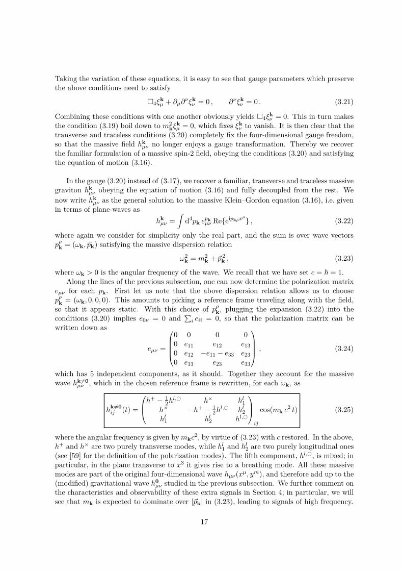
where ωk > 0 is the angular frequency of the wave. We recall that we have set c = ~ = 1.Along the lines of the previous subsection, one can now determine the polarization matrix

eµν for each pk. First let us note that the above dispersion relation allows us to choosepρ

k = (ωk, 0, 0, 0). This amounts to picking a reference frame traveling along with the field,so that it appears static. With this choice of pρ

k, plugging the expansion (3.22) into theconditions (3.20) implies e0ν = 0 and

∑

i eii = 0, so that the polarization matrix can bewritten down as

eµν =

0 0 0 00 e11 e12 e13

0 e12 −e11 − e33 e23

0 e13 e23 e33

, (3.24)

which has 5 independent components, as it should. Together they account for the massivewave hk 6=0

µν , which in the chosen reference frame is rewritten, for each ωk, as

hk 6=0ij (t) =

h+ − 12hl,# h× hl

1

h× −h+ − 12hl,# hl

2

hl1 hl

2 hl,#

ij

cos(mk c2 t) (3.25)

where the angular frequency is given by mkc2, by virtue of (3.23) with c restored. In the above,h+ and h× are two purely transverse modes, while hl

1 and hl2 are two purely longitudinal ones

(see [59] for the definition of the polarization modes). The fifth component, hl,#, is mixed; inparticular, in the plane transverse to x3 it gives rise to a breathing mode. All these massivemodes are part of the original four-dimensional wave hµν(xµ, ym), and therefore add up to the(modified) gravitational wave h0

µν studied in the previous subsection. We further comment onthe characteristics and observability of these extra signals in Section 4; in particular, we willsee that mk is expected to dominate over |~pk| in (3.23), leading to signals of high frequency.

17

4 Summary and discussion

In this paper we have addressed the following question from a comprehensive perspective:can extra dimensions induce unusual effects on gravitational waves in four dimensions, andif so how are they characterized? In this section we present our results and discuss theirobservability.

Results and comments

Starting from General Relativity with a cosmological constant in D = 4 + N dimensions onthe most generic, warped space-time geometry satisfying the background equations of motion,we have derived the wave equations (2.24) for all components of hMN (xρ, ym) from the D-dimensional linearized wave equation (2.17). We have done so by imposing the de Dondergauge condition in dimension D and then performing the reduction; we comment on differentgauge choices here after.

In the case of a background with a constant warp factor, approximating the four-dimensionalgeometry by Minkowski space-time (yielding a Ricci flat internal manifold), we have focusedon the four-dimensional gravitational wave hµν . This wave has a massless part given by itszero-mode h0

µν and a massive piece given by its non-zero modes hk 6=0µν , and it differs from usual

gravitational waves obtained from four-dimensional General Relativity in two ways:

1. The massless wave h0µν generically has an extra polarization mode on top of the “plus”

and “cross” modes of General Relativity, namely a so-called breathing mode (3.13),whose amplitude is determined by a specific scalar combination of the other components.

2. The massive tower hk 6=0µν of extra waves (3.25) have all six polarization modes turned

on, only five of them being independent, and they add up to the massless wave with adiscrete spectrum of high frequencies.

We explicitly show the zero-mode h0µν to be a free massless spin-2 wave, while the Kaluza–

Klein higher modes hk 6=0µν satisfy a standard massive equation of motion. The massless wave

being free, let us emphasize that the extra scalar h0N = (gmnhmn)0 responsible for the massless

breathing mode is absent from its equation of motion. Rather, it appears in the gaugeconditions, which we analyze in great detail for both the massless and the massive modes. Themassless wave is found to propagate only two degrees of freedom, in spite of the extra scalarwhich modifies its four-dimensional gauge conditions. This extra scalar does not transformunder a gauge transformation, and therefore cannot be removed. The massive waves hk 6=0

µν

propagate five independent degrees of freedom each, but have all polarization modes turnedon, with frequencies satisfying a massive dispersion relation.

Another important comment is that our results have been obtained by imposing thede Donder gauge in D dimensions. However, as can be checked from the expressions of Ap-pendix A.1, the above two results would remain unaltered if one starts with the D-dimensionalTransverse-Traceless gauge instead. One could also proceed without imposing any gaugechoice in D dimensions. This would lead, a priori, to more complicated equations of motionfor the zero-modes even in the Minkowskian, constant-warp factor case. Then imposing thefour-dimensional de Donder or Transverse-Traceless gauge would yield couplings among thefields in the equations of motion, and in particular between h0

µν and h0N . It would be inter-

esting to check that this leads to the same effect. In addition, this would allow to comparein detail our setup to four-dimensional scalar-tensor gravities, as motivated in footnote 6.

18

Finally, more involved cases have been studied, namely considering a non-constant warpfactor in Appendix A.2, or a more general D-dimensional Lagrangian going beyond GeneralRelativity in Appendix B. In both cases, the complete equations of motion have been derived,and corresponding new effects and complications have been discussed. In particular, for anon-constant warp factor, an interesting observation is that the four-dimensional Transverse-Traceless gauge conditions emerge naturally from the extra equations of motion, if one setsto zero the extra (vector and scalar) wave components. Despite the nice resulting framework,the four-dimensional equation remains difficult to solve: there is no simple decoupling of thevarious Kaluza–Klein modes, not even of the zero-mode. We refer to the appendices for moredetails. We now discuss to what extent the two above effects can be observed.

Observability of the effects

We now focus in more detail on the physics associated with the two effects mentioned above.We explain why they could not have been detected so far, and discuss to what extent theycould be observed in the future.

As reported, the first effect consists in having a breathing mode in the massless four-dimensional gravitational wave (3.13). This is one of the six possible polarization modes,and one of the four that General Relativity does not predict, and is thus symptomatic ofnew physics [59]. The breathing mode deforms the space in a specific manner describedby (3.15), giving a distinct signature. To observe it, one needs to disentangle it from theother two, standard, transverse modes, which requires at least three, differently orienteddetectors [59]. Currently, only the LIGO detector is active. In addition, its two sites havealmost aligned arms, which maximizes its sensitivity but allows to detect only one polarizationmode (see however [64] on detecting polarization modes of the stochastic gravitational-wavebackground). More detectors should be available in a near future.

Observing this breathing mode would also require its amplitude to be high enough. Thisamplitude is given in (3.13) for each plane wave by fN , a quantity related to the four-dimensional Fourier coefficient of h0

N = (gmnhmn)0. The latter is the zero-mode of the tracealong the extra dimensions, meaning the constant part or mean value of this trace withrespect to the extra coordinates. Then, for the breathing mode amplitude to be non-zero, onefirst needs some non-zero hmn to be emitted. This depends on the physics of the source inthe extra dimensions, on which we have no control here. Assuming some non-zero hmn, onemay wonder about taking the trace, since one is used in four-dimensional General Relativityto get traceless waves. The discussion of Section 3.1 makes it however clear that in oursetup, neither the above internal trace hN nor the four-dimensional one need to vanish; inparticular we showed that h0

N cannot be gauged away. Finally, one may wonder about theconsequences of considering the zero-mode. If the internal metric gmn is constant as for aflat torus, one considers the zero-mode of hmn itself in the trace h0

N = δmnh0mn. Whether the

latter vanishes depends again on unknown physics of the source, but we may still draw ananalogy with known four-dimensional emissions, e.g. by currently observed black hole mergers.In standard models, those produce a zero-mode of the four-dimensional wave. The latter issometimes referred to as the gravitational wave memory effect [65], which is less studied thanthe oscillatory part of the wave, perhaps because it is currently not detectable. This analogyplays in favor of an h0

mn being produced. Overall, we conclude that there is no physical reasonfor h0

N to be vanishing, generically leading to a non-zero breathing mode. An estimate of its

19

amplitude remains however out of the scope of the present study.

Let us finally emphasize that h0N is not sensitive to the size of the extra dimensions, be-

cause it is a zero-mode and it is thus independent of the extra coordinates. This is why itis here a massless mode. This is in contrast with the massive Kaluza–Klein modes, to bediscussed. Including background fluxes or curvature on the internal manifold, one may gener-ate a mass for h0

N : this could be seen using equations of Appendix B. With those equations,our analysis could be reproduced to determine whether the first effect occurs in that case.As for moduli in supergravity compactifications, such a mass should be lower than the firstKaluza–Klein mass, so it would not necessarily be related to the size of the extra dimensions.Therefore, the energy required to emit h0

N , and generate a breathing mode, needs not be high.

We turn to the second effect, corresponding to extra four-dimensional waves, that haveseveral unusual features depicted through (3.25). First, they have all six polarization modesturned on (even if only five of them are independent). More importantly, all these polarizationmodes have in each plane wave the same angular frequency ω satisfying the massive dispersionrelation (3.23), where the label k is dropped in the following. While such a dispersion relationis standard for a massive bosonic particle, it is unusual for a wave, even more so for agravitational one; we will come back to the difference between the two.9 In our framework,we are going to argue that the mass m is dominant in the dispersion relation (3.23), leadingto signals of high frequency fixed by m.

It is instructive to start by considering the background to be Minkowski times a flat torusT N . From (2.17) where the Riemann tensor vanishes, the D-dimensional gravitational wavehMN is then massless and can be decomposed into plane waves with D-dimensional light-likewave vector kM = (ω,~k3, ~kN ), satisfying ω2 = ~k 2

N +~k 23 . Looking at the four-dimensional wave

hµν and comparing to (3.23), one gets that ~k23 = ~p2 while m2 = ~k 2

N . The latter can also be

obtained as described above (3.3) by considering the Laplacian eigenvalue of ei~kN ·~y. As fora standard massless wave, the vector ~k3 corresponds to the Minkowski spatial componentsof the wave vector, and is thus associated to four-dimensional physics. For instance, physicsof black hole mergers in four dimensions have typical length scales leading to gravitationalwaves of specific wave length λ4. The latter enters the wave vector as |~k3| = 2π/λ4. In turn,the vector ~kN can be viewed as an internal momentum, and it is quantized because the torusis compact: each of its components along one circle of radius r is given by an integer times2π/r. For an average radius rN , we get an estimate |~kN | ≃ 2π/rN , which then also holdsfor the mass m. Considering more general backgrounds, these features remain true for m:it is quantized, because the spectrum of the Laplacian on a compact manifold is discrete,10

and it is given by the inverse of a typical internal length, even though the precise expressiondepends on the actual geometry. We conclude that the competition between m2 and ~p 2 inthe dispersion relation (3.23) amounts to a comparison between the wave length λ4, a typicalfour-dimensional length scale, and the typical internal length rN . As we will confirm explicitlybelow, rN ≪ λ4 so that m2 ≫ ~p 2. This implies that ω is fixed by m, and the correspondingfrequency is high compared to that associated with λ4, i.e. to the one of the massless wave.In addition, the quantization of m, related to that of the Laplacian spectrum and thus to the

9Note that the bound on the graviton mass, recently improved by LIGO [1], does not apply to waves hk6=0

µν

corresponding to Kaluza–Klein modes, as mentioned in [60]. Rather, it applies to our h0

µν , which is masslessin our setup.

10Examples of spectra on Calabi–Yau manifolds can be found in [66].

20

label k dropped so far, leads to a discrete set of frequencies.11 In summary, there is a discreteset of extra signals hk

µν , each of them dominated by a unique angular frequency ωk, which ishigh compared to that of the massless wave, and fixed by the Kaluza-Klein mass mk.

We now compute an estimate of these frequencies. We infer from above that such afrequency is given by ν = ω/(2π) = mc2/(2π~) = c/rN , where we restored the dependence onc and ~. We then need an estimate of the typical internal length rN ; a review on this topic canbe found in [22]. Current bounds from table-top experiments or missing energies in particleaccelerators are rN . 10−4 m (about 10−3 eV). Naively, this seems a high value for an upperbound on the size, with respect to e.g. what would correspond to the LHC energy. But werecall that in the picture of a three-brane, presented in the Introduction, only gravity wouldprobe the extra dimensions, while particles of the standard model would be confined to ourfour-dimensional space-time. Both sectors are in addition weakly coupled to each other. Thisvalue gives a lower bound for the frequency of ν ∼ 1012 Hz, which can still evolve according tothe considered model. The ADD models mentioned in the Introduction use n extra dimensionsto explain the hierarchy between the Planck mass Mp and another fundamental mass scalelike the electroweak one M∗, through the formula (Mp/M∗)2 = (M∗c/(2π~))n rn

N . For M∗ =1 TeV.c−2, one gets that n = 1 extra dimension is excluded, n = 2 corresponds approximatelyto the above bound, and n = 6, as in string compactifications with three-branes, gives rN ∼10−13 m, i.e. a frequency ν ∼ 1021 Hz. In any case, these frequency values are much higherthan the typical one of the recently observed gravitational waves, around 150 Hz. They arealso much higher than the upper sensitivity bound of LIGO, of the order of 103-104 Hz.In addition, future detectors seem to be planned, rather, to probe lower frequencies. Thisdisfavors the direct detection of signals with such high frequencies, which would require a newtype of apparatus. On top of being sensitive to a higher frequency range, the latter shouldhave a much smaller strain sensitivity, to get a signal-to-noise ratio comparable to LIGO: fornow this looks quite challenging. If such a detector were available, however, one could hopefor a very clean signal, since there is no known astrophysical process emitting gravitationalwaves with frequencies much greater than 103 Hz. Such high frequencies may thus be clearsymptoms of new physics.

Let us make some final comments. There is a crucial difference between the above extrasignals and a massive bosonic particle, preventing us from considering these gravitationalwaves as Kaluza–Klein gravitons. Classically, a particle is a localized object, that wouldbe detected at a definite time whenever it arrives on Earth. This does not hold for waves,which can be very spread-out objects. Realistic gravitational waves are emitted continuouslyfor a long time, by e.g. black hole binaries getting closer to each other, increasing the waveamplitude. They are then detected only when their amplitude is high enough. This brings usto comment on the amplitude of the extra signals. A priori, we have no knowledge about it, asit depends on unknown physics. However we can still make the following remark. The energyof a gravitational wave is proportional to the square of the product of its amplitude with itsfrequency. Emitting signals of high frequency would then require an important energy, unlessthe amplitude is low. We deduce that for physical waves, the higher ωk gets, the lower theamplitude is likely to be. In principle, this does not prevent the first few modes hk

µν fromhaving a reasonable amplitude. Observing such a discrete set of high frequency signals, in

11Such a relation between frequencies of gravitational waves and Kaluza–Klein masses was already mentionedin [44] where a specific Randall–Sundrum setup was considered. We comment on the analysis, partiallynumerical, of this paper at the end of Appendix A.2.

21

any polarization mode, would be a very distinct signature.

Acknowledgements

It is a pleasure to acknowledge fruitful exchanges with A. Buonanno, X. Calmet, E. Dudas,H. Godazgar, A. Harte, M. Henneaux, J. Korovins, S. Marsat, K. Mkrtchyan, R. Rahman,V. Raymond, C. Troessaert and D. Tsimpis. The research of G LG was partially supportedby the Alexander von Humboldt Foundation. Our warmest thanks go to the Deutsche BahnAG for providing us with comfortable office space in their conveniently delayed trains.

22

A Further analysis of the equations

A.1 Equations in the Transverse-Traceless gauge

In the main text, we have worked with the D-dimensional de Donder gauge (2.16). Forcompleteness, we present here a standard refinement of the latter, namely the D-dimensionalTransverse-Traceless (TT) gauge:

gP Q∇(0)P hQN = 0 , hD = 0 . (A.1)

To implement this D-dimensional gauge in the three wave equations (2.24a), (2.24b) and(2.24c), we first compute, using formulas of Section 2.2,

hD = 0 ⇔ e−2Ah4 + hN = 0 , (A.2a)

gP Q∇(0)P hQν = 0 ⇔ e−2Agπρ∇πhρν + gpq∇phqν + 2hνqgqpe−2A∂pe2A = 0 , (A.2b)

gP Q∇(0)P hQr = 0 ⇔ e−2Agπρ∇πhρr + 2e−2Ahrqgqp∂pe2A −

1

2h4e−4A∂re2A (A.2c)

+ gpq∇phqr = 0 .

Those conditions are the analogue to the de Donder ones (2.25a) and (2.25b). The three waveequations then become, in the D-dimensional TT gauge,

µν : e−2A�4hµν + ∆Mhµν − hµν∆M ln e2A (A.3a)

− 2Rπµνσgσρhρπ −

1

2e−2Agpq∂pe2A∂qe2A

(

gνµh4 − hνµe−2A)

− e−2A∇(µhν)mgmn∂ne2A − gµνhmngmrgnp

(

∇r∂pe2A +1

2e−2A∂re2A∂pe2A

)

= 0 ,

µn : e−2A�4hµn + ∆Mhµn + e−2Agpq∇phµn∂qe2A + e−2Agpq∇phqµ∂ne2A (A.3b)

+ e−2Ahµmgmp∇n∂pe2A − e−4Ahµngpq∂pe2A∂qe2A −1

2hµn∆M ln e2A

+ e−2Agpq∂µhnp∂qe2A = 0 ,

mn : e−2A�4hmn + ∆Mhmn + 2e−2Agpq∂pe2A∇qhmn + 2e−4Agpq∂pe2Ahq(m∂n)e2A (A.3c)

− 2Rsmnpgpqhqs + 2e−2Agpq∇phq(m∂n)e

2A + e−2AhN ∇n∂me2A = 0 .

The four-dimensional component hµν is not present in the two equations (A.3b) and (A.3c).The dynamics of hµn and hmn thus seem to decouple; however, one should keep in mindthe coupling present through the gauge conditions (A.2a), (A.2b) and (A.2c). Still, thecontributions of hµn and hmn can be viewed as source terms in the equations describing thedynamics of hµν . As a side remark, note that further constraints on hµn and hmn seemobtainable by tracing (A.3a).

A.2 The case of a non-constant warp factor

In the main text, we have considered the case of a constant warp factor. Let us come back hereto the study of the wave equations (2.24a), (2.24b) and (2.24c), obtained in the D-dimensionalde Donder gauge, without assuming a constant warp factor. They display an intricate mixingof hµν with the vector and scalar components, making the system of equations involved. We

23

are eventually interested in the four-dimensional dynamics, and hence in the following wefocus on a particular type of solutions, that is,

hµn = 0 , hmn = 0 . (A.4)

On top of the simplification, there are two reasons for considering (A.4). Firstly, imposingthis condition, the two equations of motion (2.24b) and (2.24c) boil down to

gπρ∇πhρν ∂ne2A = 0 , (A.5a)

h4 ∇n∂m ln e2A = 0 . (A.5b)

Tracing the last equation yields ∆M ln e2A, and on a compact manifold this Laplacian vanishesif and only if ln e2A is constant. Considering a non-constant warp factor then makes theseequations equivalent to

gπρ∇πhρν = 0 , h4 = 0 , (A.6)

i.e. the four-dimensional TT gauge. This is here equivalent to the D-dimensional TT gauge(A.1), as the latter reduces to (A.6) when imposing (A.4). Remarkably, this TT gauge fixingis enforced by the two extra equations of motion, while only the D-dimensional de Dondergauge had been imposed.12 Eventually, we are left with only the four-dimensional equation(2.24a).

Secondly, imposing (A.4) means that if one starts, rather, with equations (A.3a), (A.3b)and (A.3c), where the D-dimensional TT gauge has been imposed, then hµn and hmn act assources for hµν , as pointed-out in Appendix A.1. Imposing (A.4) then amounts to consideringthe four-dimensional equation (A.3a) without sources, which is a legitimate way to proceed;consistently, the two equations (A.3b) and (A.3c) vanish when imposing the condition (A.4).

In either case, one is left only with the study of the following four-dimensional equation:

e−2A�4hµν + ∆Mhµν − hµν

(

∆M ln e2A −1

2e−4A(∂e2A)2 +

2

3e−2AΛ4

)

= 0 , (A.7)

where (∂e2A)2 = gpq∂pe2A∂qe2A and (2.27) has been used. Furthermore, using the relation∆M ln e2A = e−2A∆Me2A − e−4A(∂e2A)2 and redefining the field as hµν = e−2Ahµν , theperturbation with respect to gµν instead of gµν , the above equation reads

�4hµν + e2A∆Mhµν + 2gpq∂phµν∂qe2A + hµν

(

3

2e−2A(∂e2A)2 −

2

3Λ4

)

= 0 . (A.8)

Finally, the internal metric can be rescaled as gmn = e−2Agmn. This is for the followingreason. The warp factor typically accounts for the backreaction of an extended object such asa Dp-brane, often present in models with extra dimensions. The Dp-branes also correspondto solutions of the equations of motion of ten-dimensional type II supergravities. So far,the background equations were assumed to be satisfied: with a non-constant warp factor,those would be solved by a Dp-brane solution. Thus we consider a D3-brane-like backgroundsolution, where the brane fills the three external space dimensions, i.e. is transverse to M.

12Suppose we do not impose the D-dimensional de Donder gauge, and keep the corresponding terms as in(2.15). Imposing then (A.4), the µn and mn components of the first order Einstein equation do not give anyrelevant condition: not a TT gauge nor a de Donder gauge.

24

This solution requires extracting the warp factor as gmn = e−2Agmn [67]. Note that thissolution also requires ingredients beyond D-dimensional gravity, namely a 5-form flux F 10

5 ,that contributes to the Einstein equation. Such contributions are studied in Appendix Band shown not to affect the discussion here below (see after (B.17)). Hence we will foregoit, and simply rescale the internal metric. The two corresponding internal Laplacians on a

scalar ϕ are then related by ∆Mϕ = e2A∆Mϕ + 12 (4 − D)gpq∂pe2A∂qϕ. Denoting (∂e2A)2 =

gpq∂pe2A∂qe2A = e−2A(∂e2A)2, (A.8) becomes

�4hµν + e4A∆Mhµν +8 − D

2e2Agpq∂phµν∂qe2A + hµν

(

3

2(∂e2A)2 −

2

3Λ4

)

= 0 . (A.9)

Whether one considers (A.7), (A.8) or (A.9), the next step requires information on theextra dimensions. We now restrict to M being compact. As presented in Section 3, this allowsone to expand, say hµν(x, y), as an infinite sum of Kaluza–Klein modes hk

µν(x) on an internalbasis as in (3.3). This leads to a set of equations for these various modes. With a constantwarp factor as in Section 3, all the modes of the four-dimensional wave decouple, each oneof them described by independent equations. In particular the zero-mode corresponds to amassless four-dimensional gravitational wave. Let us now discuss the case of a non-constantwarp factor.

In that case, the modes do not decouple in general. As we will show in detail, this can be

seen by noting the presence of ym-dependent combinations in equation (A.9) such as (∂e2A)2,which prevent one from rewriting the equation as a tower of decoupled equations for eachKaluza–Klein mode. If one insists in decoupling, considering for example the zero-modealone, i.e. a fluctuation hµν independent of the internal coordinates, the resulting equation is

�4hµν −2

3Λ4hµν = −

3

2(∂e2A)2 hµν . (A.10)

The right-hand side is then forced to be ym-independent, meaning precisely that (∂e2A)2 has tobe constant. Note that this is very unlikely for a standard non-constant warp factor. However,if this holds, the above equation would appear to describe a tachyonic field.13 Indeed, themass m on a maximally symmetric space-time is defined by the right-hand side of (A.10),

given by m2 hµν .14 This could be taken as a hint that (∂e2A)2 being constant, and the abovedecoupling, is not a sensible requirement. We now discuss this point in more detail.

For simplicity, let us consider M to be a warped flat torus T N , meaning gmn = δmn. Theinternal radii of these N circles can be reintroduced by rescaling the ym. Having a compact Mconstrains the coordinate dependence of functions, imposing specific “boundary conditions”related to the compactness: for a torus, the functions have to be periodic. Therefore, theycan be written in full generality as Fourier series. In particular, we have

hµν(x, y) =∑

k∈ZN

hkµν(x)eik·y . (A.11)

13Note that the same tachyonic behaviour appears when using, rather, (A.7) or (A.8), where for (A.7) werecall that the Laplacian of a function on a compact manifold is negative or zero.

14With such an unphysical mass definition, unitary scalars on an anti-de Sitter space-time are allowed tohave negative m

2 by the Breitenlohner–Freedman bound (an analogue on de Sitter is discussed in [68, 69]).However, it should be noted that it is not the case for massive spin-2 fields, which must have strictly positivem

2, see e.g. the review [70].

25

Each eik·y is also an eigenmode of the Laplacian, and this decomposition is the flat-torusversion of (3.3). One should now use the mode expansion (A.11) in (A.9). The result ishowever involved and eventually, one cannot easily decouple the various modes. In order toillustrate this non-decoupling, let us consider equation (A.10) for a field hµν depending on theinternal coordinates. With respect to the full equation (A.9) we are missing two terms, whichhowever would only complicate the analysis. Using the expansion (A.11), equation (A.10)becomes

∑

k

eik·y

(

�4hkµν −

2

3Λ4 hk

µν

)

+∑

k

hkµνeik·y 3

2(∂e2A)2 = 0 . (A.12)

The fact that (∂e2A)2 is y dependent, i.e. not constant, makes the last term of (A.12) differentfrom the first two: it is not written as a Fourier series. To extract from it a Fourier coefficient,we proceed as follows. We multiply (A.12) by e−in·y with a fixed n ∈ ZN , and integrate overthe torus. For a function f(x) depending on four-dimensional coordinates only, one has

∫

dy ei(k−n)·yf(x) = δ(k − n)f(x) . (A.13)

This applies to the first two terms of (A.12), where the δ-function in the sum over k fixes k

to n. We deduce that

�4hnµν −

2

3Λ4 hn

µν +∑

k

hkµν F (k − n) = 0 ∀ n , (A.14)

where

F (k − n) =3

2

∫

dy ei(k−n)·y (∂e2A)2 (A.15)

is the (k−n) Fourier coefficient of the quantity of interest. One can shift the sum to eventuallyobtain the following equation for the nth mode, in terms of the Fourier coefficients F (k):

�4hnµν −

2

3Λ4 hn

µν +∑

k

hn+kµν F (k) = 0 . (A.16)

The non-decoupling is well-illustrated by the above equation: due to the last term therein, all

the Kaluza–Klein modes enter a priori all equations, so they are completely mixed. If (∂e2A)2

were constant, only F (0) would contribute, simplifying (A.16) to

�4hnµν −

2

3Λ4 hn

µν + hnµν F (0) = 0 . (A.17)

All modes would then decouple, and the zero-mode would be tachyonic as argued earlier.15

However, (∂e2A)2 is a priori non-constant, yielding other non-zero F (k), hence the mixing.For instance, one has for the zero-mode and the nth mode

�4h0µν − 2

3Λ4 h0µν + h0

µν F (0) + hnµν F (n) +

∑

k 6=0,n

hkµν F (k) = 0 , (A.18a)

�4hnµν − 2

3Λ4 hnµν + hn

µν F (0) + h0µν F (−n) +

∑

k 6=0,−n

hn+kµν F (k) = 0 . (A.18b)

15Non-zero modes would also appear tachyonic through (A.17), but for them one should consider the twoadditional terms of (A.9).

26

One could consider a parity-invariant warp factor, so that F (n) = F (−n), and further buildinteresting combinations of modes in order to try and diagonalize the system. It remainshowever very difficult to handle the overall mixing.16 To conclude, in the case of a non-constant warp factor we seem to be unable to decouple the modes, or even to isolate one ofthem. Even though nice features are indeed present, such as the natural appearance of thefour-dimensional TT gauge conditions (A.6), we believe that the case of a non-constant warpfactor deserves a deeper study, which we leave for future work.

Let us make a final comment on related works, considering as a background the RS1model [15], discussed in the Introduction. These papers enter precisely the case describedhere: the RS1 background fits with our metric (2.18), where the four-dimensional space-timeis Minkowski, there is N = 1 extra dimension, and an explicit, non-constant, warp factor.The latter is unusual with respect to standard supergravity expressions and brane solutions,but it remains appealing here. Indeed, A is essentially linear in the extra coordinate, makingthe above (∂e2A)2 not constant but still related to the warp factor itself, which may simplifythe previous analysis. Motivated by a detection of Kaluza–Klein gravitons at the LHC, theirmass spectrum has been determined explicitly on this background in [71] (see [72] for a recentpresentation and further references). The method used is similar to the one described here,namely one starts with the five-dimensional Einstein equation, considers only hµν fluctuationsas in (A.4), and looks at the resulting first order four-dimensional equation, which shouldcorrespond to our (A.8) on Minkowski, and decomposes hµν in Kaluza–Klein modes. Further,the authors of [71] find the right decomposition such that the modes decouple, from whichone deduces the Kaluza–Klein mass spectrum. We are nevertheless unable to reproduce theiranalysis, because of a mismatch with our equation (A.8): indeed, the equations of [71] donot include a (∂e2A)2 term. Another work, [44], is motivated by relating the Kaluza–Kleinspectrum to frequencies of gravitational waves. The procedure followed there appears tobe similar, even though it is now the third term in (A.8), i.e. the one with a single ∂e2A,which seems to be missing. In addition, the spectrum is then determined partly numerically.Overall, it is unclear to us that these related works solve the issue pointed out above, evenfor a concrete background. We hope to come back to the case of a non-constant warp factor,which could lead to further effects of extra dimensions on the four-dimensional gravitationalwaves.

B Completing the model

Models with extra dimensions often contain more than D-dimensional General Relativity witha cosmological constant. In this appendix, we work-out the contributions of this additionalcontent. We start by considering the following general action:

S =1

2κD

∫

dDx√

|gD| (RD + L) , (B.1)

where L generically depends on gD MN , without containing any derivative of this metric. Thiscaptures the previous (2.1) with a cosmological constant, but also e.g. a Yang–Mills term ormore generally standard supergravities in Einstein frame, recalling that field strengths are

16It is also tempting to consider the ansatz hn6=0

µν = 0 and h0

µν 6= 0. But this leads to F (n 6= 0) = 0 in (A.18b),

i.e. to (∂e2A)2 being constant.

27

fully antisymmetrized tensors in which derivatives of the metric are absent thanks to theLevi–Civita connection. We introduce the quantities

LMN =∂L

∂gMND

, LD = gMND LMN . (B.2)

The no-derivative property allows to derive the Einstein equation without integration byparts, giving

RMN + LMN −gD MN

2(RD + L) = 0 . (B.3)

As in Section 2, we use the trace

RD =2D

D − 2

(

LD

D−

L

2

)

, (B.4)

to rewrite the Einstein equation as

RMN + LMN −gD MN

D − 2(LD − L) = 0 . (B.5)

We proceed further as in Section 2 and write the above at zeroth and first order in hMN ,

R(0)MN + L

(0)MN −

gMN

D − 2

(

L(0)D − L(0)

)

= 0 , (B.6)

R(1)MN + L

(1)MN −

gMN

D − 2

(

L(1)D − L(1)

)

−hMN

D − 2

(

L(0)D − L(0)

)

= 0 , (B.7)

whereL

(1)D = gMN L

(1)MN − gP QhQRgRSL

(0)P S . (B.8)

We now read the Ricci tensor at first order from (2.14). There, we replace R(0)MP using the

background Einstein equation (B.6). The first order Einstein equation (B.7) becomes

−1

2�

(0)D hMN + R(0)S

MNP gP QhQS + ∇(0)(M GN) (B.9)

=gMN

D − 2

(

L(1)D − L(1)

)

− L(1)MN + gP QhQ(N L

(0)M)P .

Finally, the D-dimensional de Donder gauge (2.16), to be considered from now on, makes theGN term disappear.

Constant warp factor

Let us specify here as in Section 3 to the case of a constant warp factor: we set A = 0 anddrop the tilde. The components µν and mn of (B.9) are then given by

−1

2�4hµν −

1

2∆Mhµν + Rπ

µνσgσρhρπ =gµν

D − 2

(

L(1)D − L(1)

)

− L(1)µν + gπρhρ(νL

(0)µ)π , (B.10a)

−1

2�4hmn −

1

2∆Mhmn + Rs

mnpgpqhqs =gmn

D − 2

(

L(1)D − L(1)

)

− L(1)mn + gpqhq(nL

(0)m)p , (B.10b)

using that L(0)µn = 0. Let us now consider the trace of (B.10b). It involves the Ricci tensor

R(0)mn: the latter can be replaced using the background equation of motion (B.6), leading to

−1

2�4hN −

1

2∆MhN = −gmnL(1)

mn +N

D − 2

(

L(1)D − L(1)

)

+hN

D − 2

(

L(0)D − L(0)

)

. (B.11)

28

In Section 3, considering a Minkowski background forced us to restrict to a Ricci flat in-ternal manifold. Here, the additional content allows us to consider more general Minkowskibackgrounds: see e.g. [73] and references therein for explicit examples, and [74] for a wholeclass of such backgrounds of type II supergravities. To pursue the same reasoning and getsimilar effects as in Section 3, despite a more general background, a simple condition wouldbe to have the same starting equations. This implies that the right-hand sides of (B.10a) and(B.11) should vanish. It would be interesting to check whether these two conditions hold,at least for some example. In addition, note that a Minkowski background implies through

(B.6) that L(0)µν =

gµν

D−2(L(0)D − L(0)).

General remarks and non-constant warp factor

We now make general remarks on the new contributions to the four-dimensional equation.As an illustration for those, we focus on the quantity LMN=µν , that gives rise to the term

−L(1)µν + gP QhQ(νL

(0)µ)P in (B.9). A further motivation to analyse this term is that it could

provide a mass term, i.e. a term proportional to hµν , which would be of interest for thediscussion of Appendix A.2, where the warp factor is not constant.

The background quantities should preserve four-dimensional Lorentz invariance, since weconsider an empty space-time. As a consequence, the only non-trivial four-dimensional tensorsare the four-dimensional metric, its volume form, and derivatives thereof. LMN does not

contain derivatives of the metric, so that L(0)MN=µν must be proportional to gµν . In addition,

the only possible four-dimensional background fluxes must be forms of degree 4 (or higher),proportional to the four-dimensional volume form. For instance, if L is a standard abelian

Yang–Mills term, L(0)MN=µν vanishes, because the four-dimensional 2-form field strength has

to vanish. We will make use of this general characterization.

We now consider the D-dimensional model to be a ten-dimensional type II supergravity;for conventions, we refer to [75]. A reason to do so is that this framework provides back-ground solutions with non-constant warp factor. We will eventually focus on one of them,the D3-brane. As explained in Appendix A.2, having a non-constant warp factor indicatesthe presence of an extended object such as a brane, which in turn sources a flux. Type II su-pergravities contain all such ingredients on top of gravity, and are thus suitable models here.Let us first look at contributions from the Dp-branes and orientifolds Op-planes. Those arep-dimensional extended objects, here along the three space directions of the four-dimensionalspace-time and p − 3 internal dimensions; this property prevents them from breaking four-dimensional Lorentz invariance. The part of their action that contributes to the Einsteinequation is the Dirac–Born–Infeld (DBI) action. With few assumptions, see e.g. [75], it canbe written as

SDBI = constant ×

∫

d10x e−φ√

|g10|δ(⊥)√

|g⊥|, (B.12)

where φ is the dilaton scalar field, g⊥ denotes the metric along the internal transverse direc-tions to the object and δ(⊥) localizes it in these directions. As a consequence, LMN=µν = 0for these ingredients.

The background solution of interest includes D3-branes and O3-planes. For those, thedilaton is constant and given by eφ = gs. This way, it does not contribute to the Einsteinequation, and one avoids complications related to the string versus Einstein frame. Theonly contributions left to study are thus those of fluxes. They enter LMN=µν through their

29

components having at least one leg along the four dimensions. As explained previously, thisrestricts them to be a form of degree 4 or higher. In type IIB supergravity with D3/O3,the only appropriate flux is a 5-form denoted F 10

5 . This flux is a crucial ingredient of thebackground solution, as being sourced by the D3/O3. It contributes as follows

L = −g2

s

4|F 10

5 |2 , LMN = −g2

s

4 · 4!F 10

5 MP QRSF 10 P QRS5 N , (B.13)

where for a p-form Ap, we denote |Ap|2 = Ap M1...MpAM1...Mpp /p!, raising indices with gD MN .

Its background components are either proportional to the four-dimensional volume form, or

purely internal: F10 (0)5 = F 4

5 + F5, where F 45 = g−1

s vol4 ∧ f5 with an internal 1-form f5. Inthe actual solution, f5 = e−4Ade4A = −gs ∗6 F5, even though we will not use this expression.We deduce

L(0)MN=µν = −

|g4|

4 · 3!εµρπσε ρπσ

ν |f5|2 = −|g4|

4

gµν

g4|f5|2 =

1

4gµν |f5|2 , (B.14)

where indices are raised with gκλ.

Finally, we evaluate L(1)MN=µν , considering only first order fluctuations of the metric, mean-

ing that F 105 remains at its background value. Interested in the problem of Appendix A.2, we

also set from now on hµm = hmn = 0 as in (A.4), and get

L(1)MN=µν =

|g4|

4 · 2!εµρπσε πσ

ντ gρκhκλgλτ |f5|2 . (B.15)

Since 12εµρπσε πσ

ντ = 1g4

(gµνgρτ − gµτ gρν), we conclude

L(1)MN=µν = −

1

4(gµνh4 − hµν) |f5|2 . (B.16)

We finally compute the relevant combination in (B.9) in four dimensions and obtain

− L(1)µν + gP QhQ(νL

(0)µ)P =

1

4gµν h4 . (B.17)

The terms in hµν have been canceled! In this framework and with such a background, wethus conclude that the additional content does not provide any four-dimensional mass term.In addition, given the above discussion, it seems to be a fairly general result; in particular, asimilar result holds for an F4 flux.

For completeness, we considered as well first order fluctuations of the flux. For flux

fluctuations to contribute to L(1)MN=µν in the form of a mass term, they should produce hµν ,

meaning be equal in value, as a solution to the first order equation. Despite interestingpossibilities from the flux components partially along four dimensions and along M, with aflux fluctuation weighting the square root of the hµν fluctuation, we did not find any satisfyingsolution. Flux fluctuations are subject to the flux equation of motion and Bianchi identity,which are too constraining. It would be interesting to analyse further the new contributionsto the Einstein equation.

30

References

[1] Virgo, LIGO Scientific collaboration, B. P. Abbott et al., Observation ofGravitational Waves from a Binary Black Hole Merger,Phys. Rev. Lett. 116 (2016) 061102, [1602.03837].

[2] Virgo, LIGO Scientific collaboration, B. P. Abbott et al., GW151226:Observation of Gravitational Waves from a 22-Solar-Mass Binary Black HoleCoalescence, Phys. Rev. Lett. 116 (2016) 241103, [1606.04855].

[3] R. Konoplya and A. Zhidenko, Detection of gravitational waves from black holes: Isthere a window for alternative theories?, Phys. Lett. B756 (2016) 350–353,[1602.04738].

[4] P. M. Chesler and A. Loeb, Constraining Modified Newtonian Dynamics withGravitational Waves, 1704.05116.

[5] M. Arzano and G. Calcagni, What gravity waves are telling about quantum spacetime,Phys. Rev. D93 (2016) 124065, [1604.00541].

[6] X. Calmet, I. Kuntz and S. Mohapatra, Gravitational Waves in Effective QuantumGravity, Eur. Phys. J. C76 (2016) 425, [1607.02773].

[7] C. Barceló, R. Carballo-Rubio and L. J. Garay, Gravitational echoes from macroscopicquantum gravity effects, 1701.09156.

[8] A. Kobakhidze, C. Lagger and A. Manning, Constraining noncommutative spacetimefrom GW150914, Phys. Rev. D94 (2016) 064033, [1607.03776].

[9] V. Cardoso, S. Hopper, C. F. B. Macedo, C. Palenzuela and P. Pani,Gravitational-wave signatures of exotic compact objects and of quantum corrections atthe horizon scale, Phys. Rev. D94 (2016) 084031, [1608.08637].

[10] R. Brustein, A. J. M. Medved and K. Yagi, When black holes collide: Probing theinterior composition by the spectrum of ringdown modes and emitted gravitationalwaves, 1704.05789.

[11] N. Yunes, K. Yagi and F. Pretorius, Theoretical Physics Implications of the BinaryBlack-Hole Mergers GW150914 and GW151226, Phys. Rev. D94 (2016) 084002,[1603.08955].

[12] I. Antoniadis, A Possible new dimension at a few TeV,Phys. Lett. B246 (1990) 377–384.

[13] N. Arkani-Hamed, S. Dimopoulos and G. R. Dvali, The Hierarchy problem and newdimensions at a millimeter, Phys. Lett. B429 (1998) 263–272, [hep-ph/9803315].

[14] I. Antoniadis, N. Arkani-Hamed, S. Dimopoulos and G. R. Dvali, New dimensions ata millimeter to a Fermi and superstrings at a TeV, Phys. Lett. B436 (1998) 257–263,[hep-ph/9804398].

31

[15] L. Randall and R. Sundrum, A Large mass hierarchy from a small extra dimension,Phys. Rev. Lett. 83 (1999) 3370–3373, [hep-ph/9905221].

[16] L. Randall and R. Sundrum, An Alternative to compactification,Phys. Rev. Lett. 83 (1999) 4690–4693, [hep-th/9906064].

[17] T. Appelquist, H.-C. Cheng and B. A. Dobrescu, Bounds on universal extradimensions, Phys. Rev. D64 (2001) 035002, [hep-ph/0012100].

[18] M. Graña, Flux compactifications in string theory: A Comprehensive review,Phys. Rept. 423 (2006) 91–158, [hep-th/0509003].

[19] R. Blumenhagen, B. Körs, D. Lüst and S. Stieberger, Four-dimensional StringCompactifications with D-Branes, Orientifolds and Fluxes,Phys. Rept. 445 (2007) 1–193, [hep-th/0610327].

[20] D. Andriot, E. Goi, R. Minasian and M. Petrini, Supersymmetry breaking branes onsolvmanifolds and de Sitter vacua in string theory, JHEP 05 (2011) 028, [1003.3774].

[21] U. H. Danielsson, S. S. Haque, P. Koerber, G. Shiu, T. Van Riet and T. Wrase, DeSitter hunting in a classical landscape, Fortsch. Phys. 59 (2011) 897–933, [1103.4858].

[22] M. Quiros, Introduction to extra dimensions, in Proceedings, 41st Rencontres deMoriond on Electroweak Interactions and Unified Theories: La Thuile, Val d’Aoste,Italy, Mar 11-18, 2006, pp. 200–209, 2006. hep-ph/0606153.

[23] S. B. Giddings and H. Zhang, Kaluza-Klein graviton phenomenology for warpedcompactifications, and the 750 GeV diphoton excess, Phys. Rev. D93 (2016) 115002,[1602.02793].

[24] R. Emparan and H. S. Reall, Black Holes in Higher Dimensions,Living Rev. Rel. 11 (2008) 6, [0801.3471].

[25] V. Cardoso, O. J. C. Dias and J. P. S. Lemos, Gravitational radiation inD-dimensional space-times, Phys. Rev. D67 (2003) 064026, [hep-th/0212168].

[26] E. Berti, M. Cavaglia and L. Gualtieri, Gravitational energy loss in high-energyparticle collisions: Ultrarelativistic plunge into a multidimensional black hole,Phys. Rev. D69 (2004) 124011, [hep-th/0309203].

[27] V. Cardoso, O. J. C. Dias and P. Figueras, Gravitational radiation in d>4 fromeffective field theory, Phys. Rev. D78 (2008) 105010, [0807.2261].

[28] A. Ishibashi and H. Kodama, Stability of higher dimensional Schwarzschild blackholes, Prog. Theor. Phys. 110 (2003) 901–919, [hep-th/0305185].

[29] R. A. Konoplya, Gravitational quasinormal radiation of higher dimensional blackholes, Phys. Rev. D68 (2003) 124017, [hep-th/0309030].

[30] S. Creek, O. Efthimiou, P. Kanti and K. Tamvakis, Graviton emission in the bulk froma higher-dimensional Schwarzschild black hole, Phys. Lett. B635 (2006) 39–49,[hep-th/0601126].

32

[31] A. Lopez-Ortega, Quasinormal modes of D-dimensional de Sitter spacetime,Gen. Rel. Grav. 38 (2006) 1565–1591, [gr-qc/0605027].

[32] W. G. Cook and U. Sperhake, Extraction of gravitational-wave energy in higherdimensional numerical relativity using the Weyl tensor,Class. Quant. Grav. 34 (2017) 035010, [1609.01292].

[33] P. Kanti, Black holes in theories with large extra dimensions: A Review,Int. J. Mod. Phys. A19 (2004) 4899–4951, [hep-ph/0402168].

[34] C. Cutler and K. S. Thorne, An Overview of gravitational wave sources, inProceedings, 16th International Conference on General Relativity and Gravitation:Durban, South Africa, July 15-21, 2001, pp. 72–111, 2013. gr-qc/0204090.

[35] R.-G. Cai, Z. Cao, Z.-K. Guo, S.-J. Wang and T. Yang, The Gravitational WavePhysics, 1703.00187.

[36] A. O. Barvinsky and S. N. Solodukhin, Echoing the extra dimension,Nucl. Phys. B675 (2003) 159–178, [hep-th/0307011].

[37] V. Cardoso, S. Yoshida, O. J. C. Dias and J. P. S. Lemos, Late time tails of wavepropagation in higher dimensional space-times, Phys. Rev. D68 (2003) 061503,[hep-th/0307122].

[38] Y.-Z. Chu, Gravitational Wave Memory In dS4+2n and 4D Cosmology,Class. Quant. Grav. 34 (2017) 035009, [1603.00151].

[39] Y.-Z. Chu, More On Cosmological Gravitational Waves And Their Memories,1611.00018.

[40] L.-E. Qiang, S. H. Zhao and P. Xu, Measuring the dimensionality of compact extradimensions with inspiral gravitational waves from black-hole binaries,Europhys. Lett. 116 (2016) 60001.

[41] E. Alesci and G. Montani, Can be gravitational waves markers for anextra-dimension?, Int. J. Mod. Phys. D14 (2005) 923–932, [gr-qc/0502094].

[42] C. J. Hogan, Gravitational waves from mesoscopic dynamics of the extra dimensions,Phys. Rev. Lett. 85 (2000) 2044–2047, [astro-ph/0005044].

[43] C. J. Hogan, Scales of the extra dimensions and their gravitational wave backgrounds,Phys. Rev. D62 (2000) 121302, [astro-ph/0009136].

[44] C. Clarkson and S. S. Seahra, A gravitational wave window on extra dimensions,Class. Quant. Grav. 24 (2007) F33–F40, [astro-ph/0610470].

[45] K. T. Inoue and T. Tanaka, Gravitational waves from sublunar mass primordial blackhole binaries: A New probe of extradimensions, Phys. Rev. Lett. 91 (2003) 021101,[gr-qc/0303058].

[46] M. R. DePies and C. J. Hogan, Stochastic Gravitational Wave Background from LightCosmic Strings, Phys. Rev. D75 (2007) 125006, [astro-ph/0702335].

33

[47] E. O’Callaghan, S. Chadburn, G. Geshnizjani, R. Gregory and I. Zavala, Effect ofExtra Dimensions on Gravitational Waves from Cosmic Strings,Phys. Rev. Lett. 105 (2010) 081602, [1003.4395].

[48] C. de Rham and A. J. Tolley, Gravitational waves in a codimension two braneworld,JCAP 02 (2006) 003, [hep-th/0511138].

[49] C. Deffayet and K. Menou, Probing Gravity with Spacetime Sirens,Astrophys. J. 668 (2007) 143, [0709.0003].

[50] S. P. Gomez Martnez, J. E. Madriz Aguilar and M. Bellini, Gravitational waves duringinflation in presence of a decaying cosmological parameter from a 5D vacuum theory ofgravity, Phys. Lett. B649 (2007) 343–348, [gr-qc/0703156].

[51] K. Agashe, H. Davoudiasl, G. Perez and A. Soni, Warped Gravitons at the LHC andBeyond, Phys. Rev. D76 (2007) 036006, [hep-ph/0701186].

[52] M. J. Duff, B. E. W. Nilsson and C. N. Pope, Kaluza-Klein Supergravity,Phys. Rept. 130 (1986) 1–142.

[53] D. Bailin and A. Love, KALUZA-KLEIN THEORIES,Rept. Prog. Phys. 50 (1987) 1087–1170.

[54] D. Andriot and A. Betz, β-supergravity: a ten-dimensional theory with non-geometricfluxes, and its geometric framework, JHEP 12 (2013) 083, [1306.4381].

[55] D.-M. Sjøstrøm, Bosons and Fermions in Curved Spacetime, Norwegian University ofScience and Technology (Master Thesis), 2013.

[56] P. van Nieuwenhuizen, Supergravity and the Kaluza-Klein Program Report ofWorkshop D2, Fundam. Theor. Phys. 9 (1984) 471–489.

[57] P. Van Nieuwenhuizen, AN INTRODUCTION TO SIMPLE SUPERGRAVITY ANDTHE KALUZA-KLEIN PROGRAM, in Relativity, groups and topology: Proceedings,40th Summer School of Theoretical Physics - Session 40: Les Houches, France, June27 - August 4, 1983, vol. 2, pp. 823–932, 1985.

[58] D. Andriot, G. Cacciapaglia, A. Deandrea, N. Deutschmann and D. Tsimpis, TowardsKaluza-Klein Dark Matter on Nilmanifolds, JHEP 06 (2016) 169, [1603.02289].

[59] C. M. Will, The Confrontation between General Relativity and Experiment,Living Rev. Rel. 17 (2014) 4, [1403.7377].

[60] M. Maggiore, Gravitational Waves. Vol. 1: Theory and Experiments. Oxford MasterSeries in Physics. Oxford University Press, 2007.

[61] E. C. G. Stueckelberg, Interaction energy in electrodynamics and in the field theory ofnuclear forces, Helv. Phys. Acta 11 (1938) 225–244.

[62] E. C. G. Stueckelberg, Interaction forces in electrodynamics and in the field theory ofnuclear forces, Helv. Phys. Acta 11 (1938) 299–328.

34

[63] R. Delbourgo and A. Salam, The Stuckelberg formalism for spin two,Lett. Nuovo Cim. 12 (1975) 297–299.

[64] T. Callister, A. S. Biscoveanu, N. Christensen, M. Isi, A. Matas, O. Minazzoli,T. Regimbau, M. Sakellariadou, J. Tasson and E. Thrane, Tests of General Relativitywith the Stochastic Gravitational-Wave Background, 1704.08373.

[65] M. Favata, The gravitational-wave memory effect,Class. Quant. Grav. 27 (2010) 084036, [1003.3486].

[66] V. Braun, T. Brelidze, M. R. Douglas and B. A. Ovrut, Eigenvalues andEigenfunctions of the Scalar Laplace Operator on Calabi-Yau Manifolds,JHEP 07 (2008) 120, [0805.3689].

[67] S. B. Giddings, S. Kachru and J. Polchinski, Hierarchies from fluxes in stringcompactifications, Phys. Rev. D66 (2002) 106006, [hep-th/0105097].

[68] A. Strominger, The dS / CFT correspondence, JHEP 10 (2001) 034,[hep-th/0106113].

[69] B. McInnes, Exploring the similarities of the dS / CFT and AdS / CFTcorrespondences, Nucl. Phys. B627 (2002) 311–329, [hep-th/0110062].

[70] R. Rahman and M. Taronna, From Higher Spins to Strings: A Primer, 1512.07932.

[71] H. Davoudiasl, J. L. Hewett and T. G. Rizzo, Phenomenology of the Randall-SundrumGauge Hierarchy Model, Phys. Rev. Lett. 84 (2000) 2080, [hep-ph/9909255].

[72] B. M. Dillon and V. Sanz, A Little KK Graviton at 750 GeV, 1603.09550.

[73] D. Andriot, New supersymmetric vacua on solvmanifolds, JHEP 02 (2016) 112,[1507.00014].

[74] D. Andriot, J. Blåbäck and T. Van Riet, Minkowski flux vacua of type IIsupergravities, Phys. Rev. Lett. 118 (2017) 011603, [1609.00729].

[75] D. Andriot and J. Blåbäck, Refining the boundaries of the classical de Sitter landscape,JHEP 03 (2017) 102, [1609.00385].

35