1

A Collaboration between the Wharton GIS Lab and the Center for Science and Resource Management at USGS

SILUS

WORKING

PAPER

Richard Bernknopf, Kevin Gillen, Susan Wachter

and Ann Wein

2008

Using Econometrics and Geographic Information Systems for Property Valuation:

A Spatial Hedonic Pricing Model

2

Using Econometrics and Geographic Information

Systems for Property Valuation:

A Spatial Hedonic Pricing Model

R. Bernknopf1, K. Gillen2, S. Wachter2, and A. Wein1

ABSTRACT

The hedonic pricing function approach for estimating property values uses an econometric

model. Typically, an econometric model for land values is estimated from variables that

characterize properties. Here we use the hedonic pricing function with and without spatial

explanatory variables that include distances to location amenities such as parks, central and

secondary business districts, urban growth boundaries, and environmentally sensitive locations.

Using a geographic information system (GIS), it is possible to measure distance-related

explanatory and location variables for economic applications. In this chapter, after a review of

the literature, we apply the hedonic pricing function approach to explain and estimate land

values in Miami-Dade County, Florida where environmental regulation across the county and

land preservation near national parks are contentious issues. We demonstrate that

environmental regulations and location amenities have a significant effect on land values.

Further, we demonstrate that including explanatory variables of distances measured in a GIS,

improves the model’s predictive accuracy in explaining the spatial variability of the price of

land.

1 Western Geographic Science Center, U S Geological Survey, Menlo Park, CA. 2 Wharton School, University of Pennsylvania, Philadelphia, PA

3

INTRODUCTION

There are many examples of land valuations that are informed by a particular type of

econometric model called the hedonic pricing function. This approach is an indirect or

inferential method of valuation that explains the price of a heterogeneous market good, such as

land, in terms of its valuable characteristics both within and between market segments. The

method of estimation is statistical regression analysis where the property sale transaction price

is correlated with the parcel’s characteristics to describe the market value of the parcel as a

function of the property’s physical characteristics and location amenities (Rosen, 1974,

Redfearn, 2005).

Various applications of the hedonic pricing function approach to estimating housing and land

values involve characteristics such as property listings, urban amenities, agricultural

productivity, environmental impacts, and natural and anthropogenic hazards. Studies of these

problems with econometric methods have, on occasion, included spatial explanatory variables

such as: a county boundary, an urban development boundary, or a linear distance to a central

business district (CBD) or a park. Following a review of hedonic pricing models in urban and

rural applications, we apply the method to valuing land in Miami-Dade County, Florida. Some

of the land in the county currently zoned for open space, agriculture, recreation, or vacant is

likely to be subject to development pressure and to be converted to other higher valued land

uses in the coming years. However, there is strong public interest, based on many newspaper

articles, books, and public discourse, in preserving some of these parcels in their current state

to help minimize the impacts of development on the natural environment, specifically the areas

bordering the Biscayne and Everglades National Parks. These environmentally sensitive parcels

may help protect endangered species, critical habitats and hydrologic processes that provide

ecological goods and services to the region

Within this context, the hedonic pricing function provides a useful analytical approach because

it can be used to focus on appraisal (individual) and policy (aggregate) issues (Miranowski and

Cochran, 1993). For appraisal purposes, studies establish values for specific physical and

4

location characteristics. For example, the price of a farmland parcel is indicative of its

characteristics that include productivity, soil erosion, rural amenities, access to water, and

urban density. House sales are typically analyzed to determine the price effects of location,

structure characteristics, view quality, or other intangible goods that affect the market price.

This information is important in estimating the value of a parcel for purchase or sale. The

regression equation coefficients estimated in the econometric model can be used to establish

market values for characteristics of a property like community flood mitigation. These analyses

also can provide economic information to a policy making process. When location

characteristics are influenced by public policies, hedonic studies can provide estimates of some

of the influences that a policy could have on parcel price. The terms in the hedonic equation

that represent a parcel characteristic, such as open space, can positively influence price as a

reflection of an economic benefit. Alternatively, a regulation such as an urban growth

boundary could be seen as a negative outcome because it can limit high density development

to a confined area and inhibit urban growth. This information makes it feasible to discuss and

explicitly quantify the implicit tradeoffs associated with the positive and / or negative

ramifications to a community of a proposed “smart growth” policy.

The chapter is divided into a description of the hedonic pricing approach. First there is a review

of applications followed by an explanation of the generic hedonic pricing model. Given this

context, in the next section, we developed a hedonic pricing function and incorporated it into a

Decision Support Tool (DST). The DST ranks both ecologic and economic land values for

application in development and preservation choices in Miami-Dade County. The initial

application of the DST is to assist the US National Park Service in evaluating the potential

ecological impact on Biscayne and Everglades National Parks of nearby development on the

parks. In the DST, economic land valuation considers classification of a parcel, land use, parcel

characteristics such as size, environmental regulations that affect a parcel’s potential use, and

measured distances of a parcel to specific amenities. We incorporate spatial explanatory

variables into the land market valuation and compare the estimated land price (per square

foot) with and without these variables. As will be shown, inclusion of the spatial variables

5

improves econometric estimation. In particular, the spatial variables are significant predictors

and as evidenced by measurable improvement in goodness of fit. The strengths and

weaknesses of using the hedonic pricing approach for predicting real estate prices are

described in the chapter summary.

THE HEDONIC PRICE FUNCTION

Background

The hedonic pricing function describes the relationship between the market price of a property

and its characteristics, or the services it provides. It is a method to differentiate positive and

negative characteristics of land parcel price (Bartik and Smith, 1987). The literature ascribes

the approach to multiple origins (Court, 1939, Grilliches, 1961, Lancaster, 1966, and Rosen,

1974). The method distinguishes between sources of utility, described as an assembly of

independent variables such as the number of bedrooms, air quality, soil conditions, earthquake

liquefaction potential, proximity to airports, etc., and a traded commodity, which is a

dependent variable of market price (Zilberman and Marra, 2003). Hedonic pricing statistically

divides the total price of a market good into the portions that are attributable to characteristics

not separately for sale themselves (Hanley, et al, 1997). In this way, otherwise

indistinguishable characteristics, commodities and externalities are segregated and quantified.

Applying the Hedonic Pricing Method

Hedonic valuation is performed in two stages. The first stage of the analysis measures the

market price trends for the characteristics contained in the specified equation (Beaton and

Pollock, 1992). The coefficients of the statistical regression equation are interpreted as the

“marginal prices” of the characteristics, i.e., the sum buyers would have had to pay to acquire

an additional unit of a characteristic. For example, a unit of a characteristic could be the extra

amount (marginal value) a buyer of a two-bedroom home would have to pay for an otherwise

comparable home with three bedrooms in the property market. The second stage of the

analysis incorporates the marginal prices from the first stage with additional data on buyer

incomes and tastes to specify a market demand function and characterize the market segment.

This chapter focuses on the first stage of the approach used to estimate the market price for a

6

property. To derive theoretically correct estimates of the total costs and benefits of

management and regulatory choices, the second stage would be necessary (Rosen, 1974).

A review of hedonic price function applications

The economics literature abounds with applications of the hedonic pricing approach in urban

settings with location amenities (Bartik and Smith, 1987) and in rural contexts for agricultural

land production (Miranowski and Cochran, 1993). Hedonic pricing functions also have been

used to assess how people value more intangible property characteristics such as exposure to

air and water pollution, natural hazards, and terrorist activities. The following review of the

literature is a short summary of studies that are relevant to the land valuation example in this

chapter. This review is not exhaustive nor is it intended to be; simply, it highlights the vast

literature on the subject.

The hedonic pricing method has been used extensively to estimate economic values for

ecosystem goods and services that directly affect residential property market prices (Freeman,

1993, Hanley et al., 1997, Loomis and Helfand, 2001)3. The foundation for these types of

studies is the purchaser’s willingness to pay for property that includes the quality of the local

environment as part of the consumer’s decision (Tietenberg, 1998). In general, the price of a

house is related to the characteristics of the house and property, the characteristics of the

neighborhood and community, and the environmental amenities. That is, all other things being

equal, we would expect houses and properties in neighborhoods with clean air to command

higher prices than comparable dwellings in neighborhoods with polluted air. By statistically

comparing the market values of similar properties in neighborhoods with different levels of air

quality, the analysis decomposes the aggregate property values into distinct values of the 3 Ecosystem function is an ecosystem characteristic related to the set of conditions and processes whereby an ecosystem maintains its integrity (such as primary productivity, food chain, biogeochemical cycles). Ecosystem functions include such processes as decomposition, production, nutrient cycling, and fluxes of nutrients and energy. Ecosystem services are the benefits people obtain from ecosystems. These include provisioning services such as food and water; regulating services such as flood and disease control; cultural services such as spiritual, recreational, and cultural benefits; and supporting services such as nutrient cycling that maintain the conditions for life on Earth (Millennium Ecosystem Assessment, 2003). .

7

characteristics. With adequate data on properties from several locations in a community where

the air quality varies, a regression coefficient (the marginal price of this characteristic) for air

quality can be estimated (Loomis and Helfand, 2001). As reflected by market-based housing

prices, this type of information is useful in analyzing the societal benefits of an air quality

improvement program. The coefficient provides the current willingness-to-pay for a one unit

change in air quality. The value of an incremental change in air quality is approximated by

calculating the change in house price with the change in air quality resulting from the program.

This approach works well for small changes in air quality (Loomis and Helfand, 2001). To

accurately estimate larger or non-marginal changes in environmental quality with the hedonic

model, estimation of the demand for air quality is required.

In addition to air quality, the hedonic method has been used in a variety of applications to

estimate the economic value associated with changes in environmental quality for water

pollution, noise, and other forms of negative environmental impacts. Extensive literature exists

on the estimation of the value households living in urban areas place on improving air and

water quality (Loomis and Helfand, 2001). Brookshire et al. (1982) compared the effect of

differences in sulfur dioxide and particulates levels in the atmosphere and their impact on

house prices in Los Angeles, CA. Results showed that a house in a location that has the best air

quality was worth significantly more than a house in an area with poor air quality. If the

analysis reveals a premium paid for clean air by consumers, this premium can serve as a

measure of the value of clean air to a population. Also, it has been used to assess scenic,

regional and environmental amenities, such as aesthetic views or proximity to recreational sites

(Boyle et al., 1998).

Besides the application of the hedonic pricing function to environmental issues, application to

other externalities have been undertaken in a variety of studies concerning the effect of natural

hazards and terrorism on property prices. To test the application of the expected utility model

for self-insurance, the hedonic price function was applied to earthquake hazards. Bookshire et

al. (1985) documented a housing price gradient for safety in Los Angeles and San Francisco, CA

8

for property near known earthquake faults. That is, individuals are willing to buy properties

located in more hazard-prone areas, provided that they cost less. The authors used a California

regulation based on the 1974 Alquist-Priolo Act that delineates an earthquake Special Study

Zone (SSZ) to identify parcels close to known earthquake faults for further geotechnical

analysis. Within the SSZ, residential housing prices in San Francisco, CA were negatively and

significantly correlated. The presence of the SSZ, which represents a spatial explanatory

variable, however was not significant in the Los Angeles sample. This difference could be due

to the number and locations of earthquake faults in the LA basin (faults are ubiquitous in the LA

Basin as opposed to the SF Bay region, where faults are more sparse).

In an application to volcano and earthquake hazards, Bernknopf et al. (1990) used a hedonic

function to demonstrate the negative and significant impact of hazard warning announcements

by the US Geological Survey (USGS) on real estate properties at Mammoth Lakes, CA ski resort

during the 1980’s. It was found that short term recreational visits to the area were unaffected

because consumers felt that skiing was riskier than exposure to natural hazards. However, for

real estate investment decisions, which are longer-term commitments, it was found that

property prices were affected negatively in Mammoth Lakes. In comparison to the other ski

resorts in the Western US, where there was no price response was detected.

Recently, the hedonic pricing approach has been applied to identify the effects of terrorism

attacks on property prices (Redfearn, 2005, Smith and Hallstrom, 2005). Like the

environmental and natural hazards applications described above, terrorism, among other site

amenities, is considered an external effect on the real estate market. In the Redfearn

application, housing values are expected to vary as a function of the proximity to the

externality. Relative to a comparable property that remains unaffected, it is expected that the

closer a property is to a target such as an airport the greater the property would be discounted

by the market to a lower value. This discount represents a penalty of lower value for the risk of

potential damage incurred by the impact on the surrounding neighborhood. If consumers

believe this to be true as a given expectation, the effect has been isolated and the value of

9

urban property could diminish in high population density areas. This application of the hedonic

price function tested whether there is a housing price gradient around potential terrorist

targets following the September 11, 2001 attacks. The results showed that consumers

perceived no threat from terrorism on property values, as indicated by absence of an impact on

local price indexes, sales volume or the implicit price of proximity to potential targets in Los

Angeles before and after the September 11, 2001 attacks (Redfearn, 2005).

The research undertaken by Smith and Hallstrom (2005) identified ways to design a benefit-cost

analysis of homeland security policies based on the risk of owning property in a hazardous

location. The authors suggest using the analogy of risk-related information from regional-scale

natural hazards as a gauge of how consumers would respond to changes in the risks to security.

Among the various approaches to valuing security policies, the hedonic pricing approach is

proposed as a way to measure the impact of a specific policy on the choice of risk reduction.

The analysis is based on relative property prices before and after a specific event that describes

the market value of a property. By using a regional-scale natural hazard as an analogy to a

terrorist attack, it is assumed that the scale of destruction is consistent with the impacts of a

wide-ranging, regional-scale terrorist attack on a city’s infrastructure (Smith and Hallstrom,

2005). If a major natural catastrophe were to hit a large US city the size of the losses could be

as large if not greater than the September 11, 2001 attacks. The study asserts that natural

hazards provide a reasonable parallel for estimating losses of an attack by applying benefits

transfer methods. In situations of hurricane and flooding, if the zoning criteria accurately

represent the areal extent of the likely hazard and the severity of the damaged structures, then

locations designated as inside a flood zone should reflect a reduction in value.. Areas outside

these zones should not be affected in the same way.

That said, specific natural hazard events do not affect a region uniformly. In these cases, places

are “near misses” that suffer limited wind and water damage but are not affected by the higher

intensities of a particular storm (Smith and Hallstrom, 2005). This range of non-uniformity in

locations serve as the data for the model because physical flood damage did not occur, yet

10

these places (designated as within a particular flood zone) are considered to be part of the

same market as those places that suffered losses. The approach suggests that, although the

physical damage and need for reconstruction will be less, the “near miss” locations will still

reflect perceived changes in economic value. They assert these “near misses” in a large

damaging natural hazard application is similar to a failed terrorist attack and that risk

information from the “near miss” is incorporated into and reflected by the housing market.

Data from Lee County, Florida, a “near-miss” location during hurricane Andrew, is used in the

model. In this case, Federal Emergency Management Agency designated flood zones are

included in the model to capture baseline subjective risk beliefs. The distinction of being inside

or outside of a predicted flood zone is included in the hedonic pricing model. The effect of the

risk information was statistically significant in the model and confirmed that the “near miss”

information reduced property values for homes in the region prone to coastal hazards (Smith

and Hallstrom, 2005). This suggests that the perceived risk of a hazard in a region, even if it is

not realized on the ground, still influences the real estate market. Furthermore, this example

suggests that a hedonic type model could offer a way to measure the perceived and real trade-

offs required to evaluate some types of homeland security policies.

The hedonic price function can be formulated to estimate the value of agricultural land as

reflected by its production function and ownership status. Agricultural output is a function of

labor, technique, equipment, and land. One important characteristic of land that impacts farm

productivity and affects land value is the rate and cumulative amount of soil erosion. A second

important characteristic that affects agricultural land value is geographic location, in terms of

distance, absence of nuisances (e.g., insects and other pests), and presence of exceptional

attractions (e.g., access to transportation) (Miranowski and Cochran, 1993). Other spatially

heterogeneous land characteristics that affect productive capacity such as agrochemical uptake

can influence the parcel value (Zilberman and Marra, 1993). These characteristics affect profits

and land price (Palmquist, 1989). Miranowski and Hammes (1984) have applied the approach

to explain variations in agricultural land values in terms of soil quality characteristics and the

11

impacts of soil erosion. Palmquist and Danielson (1989) considered the effects of farmland

improvements, urban density, urban growth, and rural amenities on land values.

There are additional nuances to consider as related to the ownership of the land, specifically

owner / operator of landlord / tenant situations. In an owner / operator agricultural land price

problem, Miranowski and Cochran (1993) summarize the analytical framework that supports

the empirical estimation of land price as a function of spatial heterogeneity in soil quality and

quantity characteristics. The second problem, the rental price approach for a landlord /

tenancy arrangement, valuing agricultural land is determined as a result of the actions of

demanders and suppliers of agricultural land in a particular land market. Market participants

influence the rental price by choosing specific land characteristics they prefer when they

contract for a parcel; they cannot affect the equilibrium or market-clearing price. The rental

price gets established by all of the demanders and suppliers interacting in the farmland lease

market. The renter is assumed to maximize variable profits derived from the value of the

outputs less the costs of inputs other than land (Palmquist, 1989, Miranowski and Cochran,

1993). While this is an interesting approach to using the hedonic price function, we found a

land price model by Miranowski and Cochran (1993) related more closely to the other models

reviewed and the following case study.

Building on the owner / operator agricultural land price problem, Miranowski and Cochran

(1993) develop a county-level hedonic model from location and soil characteristics data to

estimate farmland value. The empirical model includes explanatory variables for physical

characteristics including soil erodability, soil depth, average rainfall; economic activities,

including the portion of total farmland devoted to cropland, average agricultural extension

expenditure for the county, real estate tax mill rate on farmland; and spatial variables and

demographics including radial distance to the nearest metropolitan area, and population

density per square mile in the county. The authors found: (1) as topsoil depth increases, or soil

lost to erosion decreases, there is a positive effect and land value increases; (2) an increase in

erosion potential decreases land value; (3) the geographical proximity to a metropolitan area

12

was valued more in the equation relative to all other land types; (4) the effective property tax

rate had a larger than expected impact on the price of agricultural parcels; (5) help from the

public sector through increased agricultural extension activities increases land value; and (6)

counties with higher population densities should increase in land value, thereby suggesting a

possibility of a price premium due to the scarcity of agricultural land. Furthermore, the relative

share of cropland to all land was significant in reflecting differences in cropland and non-

cropland values. In sum, the review of select literature shows that hedonic models establish an

interpretation of land and property values based on both land characteristics, and non-land

characteristics. This will be extended in the following case study to include regional attributes.

The generic hedonic price model

A hedonic price function is a strategy to model an individual’s demands for a type of

heterogeneous good. There are many different versions of the same basic commodity, say,

land, and the individual generally consumes one type of property (Bartik and Smith, 1987). The

hedonic price function matches demanders and suppliers with the heterogeneous commodity

so that demand equals supply in a real estate market. Households as demanders and firms

(landlords) as suppliers of properties are assumed to be price takers, i.e., no individual can

influence the market by their actions. The method provides an estimate of the highest bids of

demanders wanting the good and the lowest offering prices of suppliers making the good

available.

A demander selects a property to maximize utility subject to the available budget and existing

prices for properties in the market. The supplier chooses a property type and number of units

to offer to maximize profits. The hedonic price function is the transformation of characteristics

to dollars. A property’s value is equal to the present discounted value of all future services

provided by that property by its current owner. There are several additional assumptions

associated with the implementation and use of the hedonic pricing model; some of the most

important ones are (Bernknopf et al., 2003):

13

• The property characteristics must vary continuously and over a considerable range of

values.

• The prices must be interpretable as value in use and not solely in terms of investment or

speculative value.

• Consumers must have similar perceptions of the property characteristics.

• The market studied must be open to migration, meaning that buyers can choose to buy

somewhere else at no disadvantage.

• The data must document the whole market under consideration; they must represent a

random sample of that market.

• The data must represent most, if not all of the characteristics that influence buyers’

decisions.

The hedonic price model in equation 1 is a statistical / econometric estimation technique that

correlates sales price with a series of independent (explanatory) variables:

1 2ln

jk

it i i i ii i

p x tα β γ= =

= + +∑ ∑ (1)

0 if time period 1 if time period i

it

i≠

= =

where lnpit is the natural logarithm of the arms-length transaction price of property i during

time period t. The hedonic price function is best estimated with sales prices for parcels of

property (built or vacant) rather than assessed values. This is because assessed or appraised

values are one step removed from a buyer’s actual willingness to pay for properties as revealed

by market prices (McFadden, 2002); xi is the location characteristics of the property that are

measured continuously, e.g., square feet of land parcel and linear distance to the central

business district, and measured categorically, e.g., land use; and ti are dummy variables

14

indicating year the transaction took place, and α, βi, and γi are the coefficients to be estimated.

In particular, the series of coefficients γi is the price index for real estate over time.

Estimation of equation 1 from available data yields regression coefficients of the model that can

be used to determine the marginal price associated with each characteristic of a property,

holding all other characteristics constant. If characteristic xi measures parcel elevation, then

the marginal price per foot due to height above sea level is the partial derivative of the price of

the property with respect to the elevation characteristics. Taking the natural logarithm of the

left (price) side of the equation suggests that the variables on the right side have multiplicative

effects on price. That is to say, if a real estate market was high (expensive) in 2005, such that

there is a large coefficient associated with that year’s index variable, then that factor should

tend to inflate the effective prices of all the relevant characteristics in that year. On the other

hand, taking the log of some of the other explanatory variables assumes that these variables do

not interact with themselves. Each additional bedroom in a house costs the same amount;

interaction would mean that the cost of each additional room would increase exponentially.

A CASE STUDY IN LAND VALUATION

Background

Miami-Dade County covers approximately 1,950 square miles in southeast Florida (Figure 1).

The county population was approximately 2.4 million and the population density was about

1,230 people per square mile in July 2006 (U.S. Census, 2007). County statistics available for

2005 report more than 928,700 housing units, about 74,260 nonfarm establishments, and

private nonfarm employment exceeded 858,000. In the application that follows, we apply the

hedonic pricing approach to value land in the dynamic development environment in Miami-

Dade County. Currently, development is encroaching on lands believed to be critical for the

survival of national parks and refuges (Hallec, 2007).

Research is underway to estimate a hedonic price function for land for use in a Decision

Support Tool. The land valuation relates market price to land use / land cover characteristics

15

indicative of conservation and development decisions in Miami-Dade County. The primary

objective of the USGS project is to develop an integrated ecological and socioeconomic land use

evaluation model for resource managers to use to reconcile the need to maintain the ecological

health of South Florida parks and refuges with the demand for land to maintain regional

economic development and community growth. With increasing pressures for higher density

development in the agricultural lands outside of the UDB, there is considerable stress on park

land and private lands adjacent to protected areas (Hallec, 2006). The research project makes

use of contributions from conservation ecology, landscape ecology, decision science, real estate

economics, environmental economics, urban planning, GIS analysis, and web technologies

(Labiosa et. al., 2008).

State, county and regional environmental regulations and management policies that restrict

development are designed to protect and preserve environmentally sensitive lands. These

same regulations and policies influence land values by altering the amount and density of land

that can be developed, which is further complicated by land use planning, zoning, and

covenants, codes and restrictions of subdivisions and home owner associations. There is

considerable debate about the future direction of development and urban expansion in Miami-

Dade County, FL, the impacts that this growth will have on lands that have been protected, and

what additional lands could be protected for present and future generations. For example,

“The most daunting threat to the Everglades is the runaway development that is still

wiping out its wetlands and stressing its aquifers. The Miami-Fort Lauderdale-West

Palm Beach conurbation has become America’s sixth-largest metropolitan area,

obliterating almost every patch of green space between the Atlantic and the perimeter

levee. Postwar Everglades suburbs such as Coral Springs, Hialeah, Miami Gardens,

Miramar, Pembroke Pines, and Sunrise have all attracted 100,000 residents, and are

approaching build-out (South Florida’s Sprawl Quickly Nearing Limit; Western Cities

Near Build-Out, by Noah Bierman and Tim Henderson, Miami Herald, 7/10/2003.).

16

Westward sprawl has become the area’s hottest political issue. Miami-Dade County has

already approved two developments outside its ”urban service boundary” – one built by

Governor Bush’s former business partner – and is now embroiled in a battle over

proposals to shift the entire boundary west and south.” p. 363 (Grunwald, M., 2006, The

Swamp: The Everglades, Florida, and the Politics of Paradise, Simon and Schuster, New

York, 450p.)

A statement by Miami-Dade County, FL in their Comprehensive Plan, which includes a different

tone concerning growth and the environment, provides insight to the public context for the

debate,

The overarching aims of the Economic Element are to expand and further diversify the

Miami-Dade economy, provide employment for all who want to work, and increase

income and wealth. More specifically, the Element provides a set of goals and

associated objectives and policies that will enhance Miami-Dade County government’s

contribution to the economic development of the area. The Element will serve as the

general policy framework for economic development decisions and it will be the guide

for operational activities, which influence economic development

(http://www.miamidade.gov/planzone/cdmp.asp).

Part of the debate concerning the effectiveness of development policies that alter otherwise

unregulated development is the economic impact of (1) creating an urban development

boundary (UDB) shown as the thick yellow-black line in Figure 1, (2) requiring land development

that is contiguous to existing development as indicated by the adjacent location of a vacant

parcel with developed land illustrated in Figure 2, (3) allowing development on land that does

not require drainage for development, and (4) avoiding ecologically sensitive lands (Figure 2

depicts protected areas located near vacant parcels that are adjacent to a developed area). In

this case study, we use the hedonic pricing method to understand how the value of

17

undeveloped land may be affected by parcel characteristics, neighborhood characteristics,

environmental regulations, location constraints, and GIS-derived spatial variables.

In addition to federal and state regulations, the overlapping mechanisms for regulating the

development of land are county and / or municipal zoning designations, subdivision regulations,

and building codes. These mechanisms can dictate such practices as type of use, parcel and

road layout, density, height, mitigation measures and setbacks from anthropogenic and

environmental landscape features. In general, zoning determines coarser-scale patterns and

design of land use, preservation and connectivity, and hence development potential. In some

jurisdictions, county or municipal officials regulate site design through stormwater

management, erosion control, and best management practices. In addition to shaping the

community’s character, aesthetic qualities and additional best management practices (beyond

county or municipal levels), subdivision regulations determine the extent to which property

owners can subdivide their property, designate minimum lot sizes, and require infrastructure

for development. Building codes set minimum standards for construction, and relate more to

the exteriors and interiors of structures and their associated systems (i.e. plumbing, electrical,

etc.).

The Miami-Dade, County government has realized that the region’s unique environmental

circumstances require special attention (http://www.miamidade.gov/planzone/cdmp.asp). As

a result, many policies and regulations have been included in Miami-Dade County’s

Comprehensive Plan to protect fragile natural resources and ensure the region’s future

sustainability. In general, the County protects environmentally sensitive lands by:

• Establishing an Urban Development Boundary

• Requiring development to be contiguous to existing development

• Only allowing development on dry land. Land can not be drained for development.

• Adhering to Florida’s State Concurrency requirements

• Administering the Environmentally Endangered Lands Program

18

Each of these protection strategies are described briefly.

Urban Development Boundary

The primary purpose of the UDB is to promote contiguous development rather than scattered,

patchy development. This helps to provide efficient delivery of public services and

infrastructure, protect environmentally sensitive land and agriculture from urban

encroachment, and promote infill/redevelopment. The UDB is included in the County

Comprehensive Plan to distinguish the area where urban development may occur through the

year 2015 from areas where it should not occur. The UDB is always under intense scrutiny to be

changed or altered to suit different groups’ needs. At its heart, the appropriate designation of

boundaries for urban containment can help provide protection and a regulatory mechanism for

preserving sensitive landscapes that are unsuitable for intensive development.

The land use planning literature suggests that the UDB should have an influence on land values.

Theoretical models consider the impact of land use policy to preserve farmland on property

values (Nelson, 1985). According to Nelson (1985), urban land value must rise because urban

containment would result in more intensive use and because benefits of urban containment

and greenbelt preservation should be capitalized in the land market. Established in 1965,

programs such as the Williamson Act in California are intended to preserve the agricultural or

open space lands by decreasing their property tax assessment (Department of Conservation,

State of California, 2008). If urban containment is effective, the land market will value

proximity to the boundary. Near the boundary, property owners can take advantage of the

views and privacy of the greenbelt beyond the UDB. This is a rural amenity effect (Hellerstein et

al., 2002). Below we evaluate whether land values outside the UDB are systematically lower

than land values inside the boundary.

Contiguous Urban Development Requirement

19

It is both Miami-Dade County and State of Florida policy to prevent leapfrog or patchy

development. Several policies encourage local decision-makers to deny development projects

that are not contiguous to other development projects. This policy requirement complements

the purpose of the UDB to concentrate development in certain areas.

No Drainage Policy

Miami-Dade County’s environmental regulation prohibits draining wetlands for development.

State and County Concurrency Requirements

Concurrency has its roots in state legislation called the Local Government Comprehensive

Planning and Land Development Regulation Act, which was adopted by the Florida legislature in

1985 and amended Chapter 163, Florida Statutes. The act mandated that specific level of

service standards be adopted for roadways, mass transit, water, sewer, solid waste, local

recreation open space and drainage, and that each of these services be defined and addressed

in local comprehensive plans. Also, it further stated that no development orders can be issued

when the adopted levels of service would not be met.

Environmentally Endangered Lands Program

The Environmentally Endangered Lands (EEL) Program has been established to acquire,

preserve, enhance, restore, conserve, and maintain threatened natural forest and wetland

communities located in Miami-Dade County, for the benefit of present and future generations.

(Ord. No. 04-214, §§ 1, 5, 12-2-04) The purpose of the EEL Program is to acquire and protect

environmentally-endangered lands which, if not acquired, would threaten the environmental

integrity of the existing resource, or which, if acquired, would enhance the environmental

integrity of the resource with the primary objective of maintaining and preserving their natural

resource values for present and future generations.

A hedonic model for land valuation in Miami-Dade County, Florida

20

We estimated land value in Miami-Dade County, FL as a function of parcel square footage,

zoning and environmental regulations, location and distance to amenities, and year and season

of property transaction. We demonstrate that, consistent with planning concepts, theory in the

literature, land use controls have an impact on potential land values inside and outside the UDB

and around other environmentally sensitive and protected land. Further, an important

contribution to the spatial variation in price is the measured distances from a parcel to a variety

of amenities.

Study Area, Data and Variables

Property data were aquired from the Miami-Dade County tax roll. We obtained comprehensive

information for every unique parcel amounting to 541,184 observations. Table 1 summarizes

the real estate statistics for Miami-Dade in the data set. Of the total number of parcels,

undeveloped land parcels in the county accounted for approximately 51,000 observations.

There were about 28,500 observations of arms-length transactions. The final data set consists

of about 24,000 observations after removing statistical outliers4 and observations with missing

or incorrect data.

Table 1: Summary Statistics for properties in Miami-Dade County, Florida in 2006

# of

Parcels Sq ft Sale price

Assessed

Value

$/Sq

ft

Total Parcels 541,184

Total Vacant 50,850

Vacant inside UDB 30,739 26,399 14,117 25,238

Vacant non-UDB 20,111 18,739 9,991 19,454

Average size inside UDB 71,208 74,850

Average size non-UDB 523,590

557,90

2

4 Outliers were defined as observations which lay in the 2.5% tails of any variable’s distribution.

21

Average Sale Price inside UDB

1,592,88

2

21.2

8

Average Sale Price on-UDB 583,168 1.05

Median Sale Price inside UDB 240,000 3.21

Median Sale Price non-UDB 25,000 0.05

Average Assessed Price inside

UDB 252,664

3.38

Average Assessed Price non-UDB 100,457 0.18

Median Assessed Price inside UDB 81,445 1.09

Median Assessed Price non-UDB 9,615 0.02

Table 1 lists statistics for parcels inside the UDB and non-UDB (outside the UDB). There is a

considerable disparity between parcels located inside and outside of the UDB for both in size

and in sale price and assessed price and in price per sq ft. A parcel located inside the UDB is

slightly less than 13.5% the size (sq ft.) and has an average sale price that is 20 times greater

and a median sales price that is over 60 times greater than a parcel outside the UDB. The

assessed values in Table 1 show the same order of magnitude difference as the sale price, i.e.,

the average and median assessed price are 19 and 54 times greater respectively, inside the UDB

relative to outside the UDB. This price differential between parcels inside and outside the UDB

has a significant impact on predicting the value of vacant land in the hedonic model.

Depending on consumer preferences, each variable is anticipated to have either a positive or

negative effect on price in the following ways. We hypothesize that lot size is negatively

correlated with price because as a parcel size increases, a buyer’s marginal willingness to pay

will decline on a price per square foot basis while the total price of the property increases.

Land zoning influences are expected to be positive for agricultural lands and negative for

recreational parcels. We hypothesize that a recreation zoning is worth less because it is

perceived to have a lower probability of conversion to a higher (developed) land use. We

expect the opposite for agriculturally zoned parcels. “Transacted in Winter Months” is expected

22

to be negatively correlated with price because real estate transactions traditionally are less

likely in those months even in Florida.

GIS provides the important capability to use the location of amenities and measures of distance

as explanatory variables that identify land use and land cover, and to visualize parcel

characteristics. The land use map shown in Figure 2 illustrates where a parcel is located relative

to the location of some spatial amenities. The GIS data are used to represent development

restrictions and boundaries based on environmental regulations and flood zones. We expect

properties located inside the UDB (shown as the yellow-black boundary line in Figure 1) and

properties that are contiguous to existing development (shown, for example, as the gray-black

bounded areas have been proposed for urban expansion) to have positive effects on property

values. Locations within the UDB should be positively correlated with price because land within

the UDB is supported by significant public infrastructure and greater development density is

permitted inside the boundary. A parcel contiguous to development satisfies a regulatory

requirement and should be worth more than parcels located away from existing development.

We expect rural and urban amenities such as proximity to the ocean and environmentally

sensitive parcels to have positive effects on land values. EEL is identified, publicly listed for

preservation and purchased as part of a county land acquisition program (Code of Ordinances,

Miami-Dade County, Florida, Chapter 24-50). An EEL listing requires agreement by the owner.

Parcels marked for EEL designation would lower the probability of conversion to developed

land, because there is an expressed desire to protect the land.

The spatial variables include distances to central business districts, highways, parks, and

waterways. We anticipate both positive and negative impacts on the sales price depending on

the variable. The variable, Distance to the Miami CBD, is the Euclidean distance (in miles) from

a parcel to the Miami Central Business District (CBD). We expect that the farther a parcel is

from the city center, the greater the negative effect on land price. The distance to nearest

secondary CBD variable is expected to be positively correlated to price as a convenience to

residents. However, the primary CBD may have a dominating effect. Distance to Nearest

23

Highway (in miles) is hypothesized to have a negative correlation with price suggesting

properties closer to highways are more valuable. Distance to Park (in miles) is a parcel’s

Euclidean distance to a park other than a national park and is hypothesized to be inversely

correlated with price. We anticipate that the distance to a park, (including a national park) to

be negatively correlated with price, i.e. the closer the parcel is to a park, the more valuable the

parcel is to the buyer. We hypothesize Distance to Canal (in miles) to be positively correlated

with price; price should increase the farther the parcel is from a canal. Some canals can contain

contaminated water that can influence the value of nearby properties. We also realize that

there could be canals that are desirable (e.g., for navigation). The variable Distance to Nearest

Iinland Body of Water (in miles) should be positively correlated with price because these bodies

of water are caused by extraction of construction materials that then fill with undesirable

mineralized water. Parcels west of canal L31 are hypothesized to be less valuable than parcels

east of the Canal because this particular canal separates parcels that are protected from

flooding from those that are not (Dwyer, 2007). A high potential for flooding is posited to have

a negative effect on parcel price because of the no drainage rule, which does not allow for the

dewatering of a parcel. Likewise, the coastal flooding variable is expected to have a negative

coefficient because these parcel values would be discounted in response to the coastal flooding

hazard. Ocean side properties are hypothesized to have a positive correlation with land price

because locations near the ocean are desirable for views and access.

All of the explanatory variables were evaluated for inclusion in the model. Table 2 lists the

dependent and all of the explanatory variables for each parcel in the county that could be

included in the hedonic price function. Table 3 contains the salient statistics for the dependent

and the explanatory variables.

The relationships of a parcel and its characteristics to other nearby parcels and their

characteristics can help explain spatial price differentials. In combination, the visualization of

land use in Figure 2 and the characteristics listed in Table 3 provide a “picture” of the real

24

estate market for land in Miami-Dade County. In this way, GIS adds a new dimension to the

economic valuation of properties using the hedonic pricing approach.

Model specification

We apply the log-semilog formulation of the hedonic price function. Several variants of the

statistical regression were run to test its robustness to different model specifications, different

data reconciliation choices, and different ways of representing urban development and

environmental regulations5. The hedonic price function for Miami-Dade County combines

elements from all of the types of applications identified and described in the literature review.

Integration of these elements with distance and location explanatory variables along with other

parcel characteristics provides a way to achieve more robust estimates of land value. As part of

the development of the valuation model, we are able to evaluate whether the location

variables derived in a GIS are intuitive and increase the explanatory power to help improve the

model (Sandberg, 2004, Xu, 2007).

The hedonic price function for land in Miami-Dade County is

1 2 3ln ip H Y Z Tτ τα β β β γ= + + + + (2)

where ln ip τ is the natural log of the transaction price per square foot of property i during time

period ( ), 1,..., nτ τ = ; ( )1,..., iH h h= and ( )1,..., iY y y= are property characteristics with hi

measured continuously, e.g., square feet of land parcel, yi measured categorically, land use,

( )1,..., iZ z z= variables measured continuously as linear distances (in miles), e.g., distance to

the central business district; and T are fixed effect variables indicating whether the transaction

takes place during time period t, and α, βj, and τγ are the coefficients to be estimated. In

5 The hedonic pricing literature addresses but does not resolve the question of functional form. A general principle of statistics asserts that it is best to have a logical, maximum form in place a priori so that the available data can be devoted to fitting and testing that form rather than to finding a form. To counteract the danger of “overfitting” data and coming up with meaningless or skewed results, the reliability of the model can be tested.

25

particular, the series of coefficients τγ are the price indices. The model is estimated with and

without the spatial explanatory variables for the Miami-Dade County data.

Table 2: Variables and definitions in the hedonic price function for Miami-Dade County, FL.

VARIABLE Definition

price_sqft Lot price in dollars per square foot

AREA Lot area in square feet

PERIMETER Lot exterior perimeter in feet

LOT_SIZE Lot size of each parcel in square feet

xlot_sqft Lot square footage is the size of each parcel in square feet

Winter

Real estate transaction occurred during the winter months, =1 if

transacted in winter months

year_19XX

A parcel sale occurs in a specific year, =1 if transaction occurs in the

given year

Recreational*

Recreational encompasses all parcels designated as zoned

“recreational” in the Miami-Dade County Land Use map,

=1 if zoned "recreational"

Agricultural

Agricultural encompasses all parcels designated as zoned

“agricultural” in the Miami-Dade County Land Use map,

=1 if zoned "agricultural"

Flood_zone =1 if coastal flood zone

EEL_Private

A parcel is designated as an Environmentally Endangered Land if it

has ecologically desirable characteristics that the landowner and the

county have agreed to not develop, =1 if parcel is private EEL

purchase

Dist_CBD**

Distance to CBD is the linear distance in miles from the Miami Central

Business District to the parcel

using a GIS

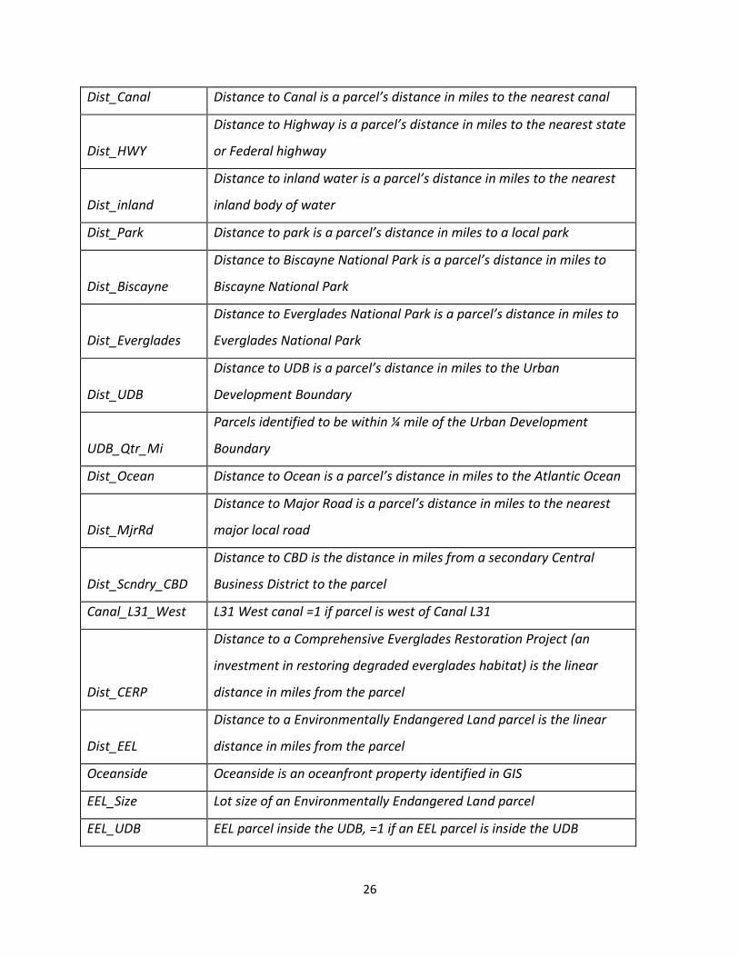
26

Dist_Canal Distance to Canal is a parcel’s distance in miles to the nearest canal

Dist_HWY

Distance to Highway is a parcel’s distance in miles to the nearest state

or Federal highway

Dist_inland

Distance to inland water is a parcel’s distance in miles to the nearest

inland body of water

Dist_Park Distance to park is a parcel’s distance in miles to a local park

Dist_Biscayne

Distance to Biscayne National Park is a parcel’s distance in miles to

Biscayne National Park

Dist_Everglades

Distance to Everglades National Park is a parcel’s distance in miles to

Everglades National Park

Dist_UDB

Distance to UDB is a parcel’s distance in miles to the Urban

Development Boundary

UDB_Qtr_Mi

Parcels identified to be within ¼ mile of the Urban Development

Boundary

Dist_Ocean Distance to Ocean is a parcel’s distance in miles to the Atlantic Ocean

Dist_MjrRd

Distance to Major Road is a parcel’s distance in miles to the nearest

major local road

Dist_Scndry_CBD

Distance to CBD is the distance in miles from a secondary Central

Business District to the parcel

Canal_L31_West L31 West canal =1 if parcel is west of Canal L31

Dist_CERP

Distance to a Comprehensive Everglades Restoration Project (an

investment in restoring degraded everglades habitat) is the linear

distance in miles from the parcel

Dist_EEL

Distance to a Environmentally Endangered Land parcel is the linear

distance in miles from the parcel

Oceanside Oceanside is an oceanfront property identified in GIS

EEL_Size Lot size of an Environmentally Endangered Land parcel

EEL_UDB EEL parcel inside the UDB, =1 if an EEL parcel is inside the UDB

27

Canal

UDB***

Parcel is designated as inside the Miami-Dade County’s Urban

Development Boundary,=1 if parcel is within Urban Development

Boundary

Contiguous

A parcel is designated as contiguous for development if it is located

to an existing developed parcel, =1 if parcel is contiguous to

development

Zone_A

Zone A is the flood insurance rate zone that corresponds to the 1-

percent annual chance floodplains that are determined in the Flood

Insurance Study by approximate methods of analysis. Mandatory

flood insurance purchase requirements apply.

Zone_AE

Zone AE is the flood insurance rate zone that corresponds to the 1-

percent annual chance floodplains that are determined in the Flood

Insurance Study by detailed methods of elevation analysis.

Mandatory flood insurance purchase requirements apply.

Zone_AH

Zone AH is the flood insurance rate zone that corresponds to the

areas of 1-percent annual chance of shallow flooding with a constant

water-surface elevation (usually areas of ponding) where average

depths are between 1 and 3 feet. Mandatory flood insurance

purchase requirements apply.

Zone_VE

Zone VE is the flood insurance rate zone that corresponds to areas

within the 1-percent annual chance coastal floodplain that have

additional hazards associated with storm waves. Base Flood

Elevations derived from the detailed hydraulic analyses are shown at

selected intervals within this zone. Mandatory flood insurance

purchase requirements apply.

Zone_X500

Zone X is the flood insurance rate zone that correspond to areas

outside the 1-percent annual chance floodplain, areas of 1-percent

annual chance sheet flow flooding where average depths are less

28

than 1 foot, areas of 1-percent annual chance stream flooding where

the contributing drainage area is less than

1 square mile, or areas protected from the 1-percent annual chance

flood by levees. No Base Flood Elevations or depths are shown within

this zone. Insurance purchase is not required in these zones.

Flood_zone_inland

Inland flood zone is measured as the proximity to the ocean-caused

coastal flooding, which is within a half mile of the shoreline

* Bold font indicates a non-spatial regulatory variable

** Italic font indicates a spatial variable measured in a GIS

*** Bold italic font indicates a spatially-measured regulatory variable

Table 3: Statistics for the dependent and explanatory variables in the hedonic price function for

Miami-Dade County, FL.

VARIABLE N MIN MAX MEAN STD Deviation

AREA 24224 19.869 97208597 194207.9 1110742

price_sqft 24127 0.010099 993.6655 21.66898 64.22064

PERIMETER 24224 29.571 58257.65 1291.744 1904.62

LOT_SIZE 24224 0.5 7907838 26170.98 175847.1

lot_sqft 24224 8 94050396 199601.3 1138525

Recreational 24224 0 1 0.000991 0.031461

Agricultural 24224 0 1 0.012178 0.109682

Flood_zone 24224 0 1 0.634412 0.481605

EEL_Private 24224 0 1 0.051148 0.220303

Dist_Canal 24224 0 5.82 1.079939 0.959757

Dist_HWY 24224 0 10.38 1.331828 1.755592

Dist_Park 24224 0 12.77 2.010266 2.33851

Dist_Biscayne 24224 0 24.8 11.23411 5.039312

Dist_Everglades 24224 0 27.81 9.765871 7.371954

29

Dist_UDB 24224 0 13.74 1.513842 2.697697

UDB_Qtr_Mi 24224 0 1 0.0534 0.2248

Dist_Ocean 24224 0 24.08 6.8902 5.816657

Dist_MjrRd 24224 0 2.75 0.124106 0.337726

Dist_Water 24224 0 5.95 0.536313 0.604201

Dist_CBD 24224 0.035 41.07 15.36 9.32

Dist_Scndry_CBD 24224 0 15 3.076701 2.916524

Canal_L31_West 24224 0 1 0.157117 0.363918

Dist_CERP 24224 0 15 5.17301 3.848523

Dist_EEL 24224 0 15 2.860882 2.840016

Oceanside 24224 0 1 0.129004 0.335212

EEL_Size 24224 0 27693706 36423.03 452665.1

EEL_UDB 24224 0 1 0.008132 0.089814

Canal 24224 0 1 0.040208 0.196451

UDB 24224 0 1 0.605 0.489

Contiguous 24224 0 1 0.110964 0.314094

Zone_A 24224 0 1 0.160213 0.366811

Zone_AE 24224 0 1 0.192454 0.394236

Zone_AH 24224 0 1 0.27803 0.448038

Zone_VE 24224 0 1 0.003715 0.060841

Zone_X500 24224 0 1 0.058909 0.235458

Flood_zone_inland 24224 0 1 0.123803 0.329363

year_1970 24224 0 1 0.000165 0.012849

year_1971 24224 0 1 0.003179 0.056291

year_1972 24224 0 1 0.004046 0.063477

year_1973 24224 0 1 0.012219 0.109866

year_1974 24224 0 1 0.017792 0.132198

year_1975 24224 0 1 0.01193 0.108575

year_1976 24224 0 1 0.017834 0.132349

30

year_1977 24224 0 1 0.018246 0.133844

year_1978 24224 0 1 0.016595 0.127751

year_1979 24224 0 1 0.014985 0.121496

year_1980 24224 0 1 0.026626 0.160993

year_1981 24224 0 1 0.021797 0.146022

year_1982 24224 0 1 0.015481 0.123456

year_1983 24224 0 1 0.014283 0.118659

year_1984 24224 0 1 0.014614 0.120003

year_1985 24224 0 1 0.015687 0.124264

year_1986 24224 0 1 0.015481 0.123456

year_1987 24224 0 1 0.014325 0.118828

year_1988 24224 0 1 0.01643 0.127125

year_1989 24224 0 1 0.018205 0.133695

year_1990 24224 0 1 0.016058 0.125703

year_1991 24224 0 1 0.017132 0.129765

year_1992 24224 0 1 0.015357 0.122969

year_1993 24224 0 1 0.018907 0.136199

year_1994 24224 0 1 0.022746 0.149096

year_1995 24224 0 1 0.018081 0.133248

year_1996 24224 0 1 0.020558 0.141902

year_1997 24224 0 1 0.025471 0.157553

year_1998 24224 0 1 0.029475 0.169137

year_1999 24224 0 1 0.033025 0.178706

year_2000 24224 0 1 0.039837 0.195579

year_2001 24224 0 1 0.042272 0.201213

year_2002 24224 0 1 0.059693 0.236922

year_2003 24224 0 1 0.092512 0.289753

year_2004 24224 0 1 0.11245 0.315926

year_2005 24224 0 1 0.118271 0.322936

31

year_2006 24224 0 1 0.028236 0.165651

32

Model results

Two regression equation models were estimated and they performed as expected. The

dependent variable for both models is

ln priceft 2

and the estimation method to explain the

variation in land price is ordinary least squares. The results for Model 1, a nonspatial version of

the hedonic price function, are listed in the four left columns in Table 4 that includes property

characteristics, land zoning, and sale year. Model 2 results, a spatial version of the hedonic

price function, are contained in the columns on the right side of Table 4 (Model 2 includes

Model 1 variables). Addition of the spatial explanatory variables (see Table 2 for which

variables are coded as spatial) in Model 2 enhances the nonspatial model with distance

measurements from a parcel to a variety of amenities and destinations, and delineation of

environmental and growth regulations and standards. The explanatory power of Model 2 is

more than twice that of Model 1, i.e., the adjusted R2 rises from about 0.34 to about 0.77.

Further a significant number of the GIS measured explanatory variables are statistically

significant (Pr < .01) to improve the hedonic valuation of the Miami-Dade County land market.

The Model 1 variables that performed as expected were lot size and environmentally

endangered land. Lot size measured as lot square footage and EEL have the expected sign and

are statistically significant.

Table 4: Regression results for the hedonic price nonspatial and spatial models*

Model Model 1: Excludes Spatial Explanatory Model 2: Includes Spatial Explanatory

33

Variables;

adjusted R2 = 0.3352 Variables;

adjusted R2 = 0.7683

Variable

Estimate

Error

T value Pr > |t| Estimate Error t Value Pr > |t|

Intercept -1.29076 0.99461 -1.3 0.1944 -1.09794 0.58801 -1.87 0.0619

Lot_sqft

-2.53E-07

1.13E-08

-22.34 <.0001 -6.91E-09 6.76E-09 -10.23 <.0001

Flood_zone 0.79381 0.21058 3.77 0.0002 -0.82635 0.1265 -6.53 <.0001

Recreational -.24303 0.40674 -0.6 0.5502 -0.68378 0.23946 -2.86 0.0043

Agricultural -1.0501 0.11666 -9.0 <.0001 0.24256 0.06964 3.48 0.0005

EEL_private -1.88146 0.14145 -13.3 <.0001 -0.70475 0.08686 -8.11 <.0001

Dist_CBD -0.07466 0.00165 -45.26 <.0001

Dist_Canal 0.0278 0.01041 2.67 0.0076

Dist_Water 0.14813 0.01834 8.08 <.0001

Dist_HWY -0.06415 0.00776 -8.27 <.0001

Dist_Everglades -0.00558 0.00234 -2.38 0.0172

Dist_Scndry_CBD 0.07062 0.00704 10.03 <.0001

Canal_L31_West -0.66027 0.04186 -15.77 <.0001

Dist_EEL -0.08386 0.00647 -12.96 <.0001

Oceanside 0.96204 0.02917 32.98 <.0001

UDB_Qtr_Mi -0.29458 0.03487 -5.87 <.0001

UDB 1.85972 0.02935 63.36 <.0001

Contiguous 0.40938 0.0187 21.9 <.0001

Year_1981 0.13933 0.99836 0.14 0.889 1.0468 0.58775 1.78 0.0749

Year_1983 0.77995 1.00034 0.78 0.4356 1.00454 0.58889 1.71 0.0881

Year_1984 0.98356 1.00021 0.98 0.3254 1.27435 0.5888 2.16 0.0304

Year_1985 1.03367 0.99986 1.03 0.3012 1.11276 0.5886 1.89 0.0587

Year_1986 1.26586 1.00005 1.27 0.2056 1.3149 0.58871 2.23 0.0255

Year_1987 1.17613 1.0003 1.18 0.2397 1.29243 0.5888 2.19 0.0282

Year_1988 1.3414 0.99958 1.34 0.1796 1.42426 0.58846 2.42 0.0155

Year_1989 0.93626 0.99909 0.94 0.3487 1.36329 0.58816 2.32 0.0205

Year_1990 1.21352 0.99975 1.21 0.2248 1.42193 0.58855 2.42 0.0157

Year_1992 1.55093 1.0001 1.55 0.121 1.32121 0.58874 2.24 0.0248

Year_1993 1.9065 0.99892 1.91 0.0563 1.46483 0.58804 2.48 0.013

34

Year_1994 1.7666 0.9982 1.77 0.0768 1.4684 0.58765 2.5 0.0125

Year_1995 1.97575 0.99914 1.98 0.048 1.46483 0.58819 2.49 0.0128

Year_1996 2.19656 0.99857 2.2 0.0278 1.57375 0.58783 2.68 0.0074

Year_1997 2.16248 0.99781 2.17 0.0302 1.63725 0.58738 2.79 0.0053

Year_1998 2.44851 0.99737 2.45 0.0141 1.72018 0.58713 2.93 0.0034

Year_1999 2.42212 0.99707 2.43 0.0151 1.71521 0.587 2.92 0.0035

Year_2000 2.49168 0.99665 2.5 0.0124 1.72573 0.58671 2.94 0.0033

Year_2001 2.73561 0.99653 2.75 0.0061 1.78815 0.58666 3.05 0.0023

Year_2002 2.70334 0.99596 2.71 0.0066 1.84433 0.5863 3.15 0.0017

Year_2003 2.96231 0.99547 2.98 0.0029 2.05272 0.58602 3.5 0.0005

Year_2004 3.45777 0.99532 3.47 0.0005 2.38655 0.58594 4.07 <.0001

Year_2005 3.69459 0.99528 3.71 0.0002 2.62069 0.58592 4.47 <.0001

Year_2006 4.07573 0.99754 4.09 <.0001 3.06471 0.58724 5.22 <.0001

*All variables are significant at least at the 10% level.

However, other explanatory variables behaved non-intuitively, including land zoned for

recreation and agriculture and coastal flooding potential. We found the zoning variable for

recreation had the intuitive sign but was statistically insignificant, while the agriculture zoning

for land use had the non-intuitive sign, although less negative than recreation, and was

statistically significant. The flood zone variable was non-intuitive, in that the value of a

property was found to increase when subject to coastal flooding. One of the best predictors

was the transaction year fixed effect for transactions that occurred between 1981 and 2006.

They were found to be positively related for market conditions that prevailed in that year.

Overall, the result for Model 1 is disappointing because of the low explanatory power, and the

lack of evidence for the importance of the zoning variables as drivers in the real estate market

for conversion of land parcels to higher uses.

The results for Model 2 produce a substantial improvement over Model 1 due, in part, to the

change from non-intuitive results for specific explanatory variables in Model 1 to intuitive

results in Model 2 and the dramatic increase in explanatory power. As in Model 1, the lot size

measured as square footage has the intuitive sign and is statistically significant. The remaining

35

parcel-characteristic variables performed as hypothesized in Model 2. These variables are the

recreation and agriculture zone variables had opposite signs and were significant. Land zoned

recreational is negatively correlated with price and land zoned agricultural is positively

correlated, suggesting that agricultural lands are higher valued by the market. Also, parcels

subject to coastal flooding changed signs to have a negative impact on price. This could suggest

that the variable of Model 1 could have been confounded by distance to the ocean

(dist_ocean), which was isolated in Model 2 and not found to be significant.

The eleven spatial and two spatial-regulatory variables that were derived and measured using

GIS add a new dimension to the hedonic price function. The effects of the two spatial

regulatory variables (Parcel is Located Within the UDB and Parcel is Contiguous to Development)

are positively correlated with price as expected. The effect is quite large and can be observed

in Figure 3 for land parcels near the UDB. As the map shows, the predicted price from the

equation for all vacant parcels displays how the price declines if the parcel is located outside

the UDB (in Figure 3, the UDB is the red boundary line). Like Model 1, the EEL is negatively

correlated with price and significant. The price is being discounted because the parcel has been

designated environmentally endangered by the county, e.g., a critical habitat. Turning to the

eleven spatial variables, the ocean side properties variable performed as expected. That is,

oceanfront properties are positively correlated with price. The variable Parcels West of Canal

L31 is intuitive and statistically significant due to the fact that parcels west of the canal are not

flood protected. Distance to Nearest Inland Body of Water is positively correlated with the land

price. This variable confirms that distance from these potentially contaminated bodies of water

matters. The variable, Distance to Miami CBD, is negatively correlated and significant. The

influence of this variable can be seen in Figures 3 and 4. As the map in Figure 3 shows, the

predicted price from the equation can be plotted to show that prices decline if the parcel is

located farther away from the CBD. This is confirmed on the graph of the bid-rent curve in

Figure 4 that shows a steep decline in price with increasing distance from the Miami CBD. The

variable Distance to Canal is ambiguous because not all canals are undesirable. Distance to

Nearest Highway (in miles) is intuitive and is negatively correlated with price. Distances to the

36

two national parks are negatively correlated with price. However, only the Distance to

Everglades National Park is statistically significant. Distance to Nearest Secondary CBD is

positively correlated with price and intuitive. UDB_Qtr_Mi is negatively correlated with price.

The variable is ambiguous because properties within 14 mile and inside the UDB would be

valued more highly than properties outside the regulatory boundary. Distance to Park is

positively correlated with price but statistically insignificant.

To consider the discussion of the results of Model 2, there are five categories of explanatory

variables in Model 2 that fit into the parcel, regulatory, spatial, and spatial-regulatory

framework, namely hazards, amenities, and measured distances. The explanatory variables

have different effects on land price. Parcel size measured in total square feet contributes a

very small negative decrease to price per square foot of -0.000007, which translates to a

percent value of -0.0007%.6 A parcel location inside the UDB (+ 183%) and contiguous

development (+ 42%) increase land price by a combined 225%. An agricultural zoning increase

price by 24%, while a recreation zoning designation (- 69%) and an EEL listing (-70%) reduce

price by 138%. [Is there a variable missing in the last phrase? . This demonstrates the tradeoffs

of different zoning characteristics in the land market. Environmental amenities, as expressed

through regulations, have a significant impact in determining a parcel land value. The hazards

variables of coastal flooding (- 83%) and the L31 Canal (- 67%) were negative and reduce price

by a combined 150%. The location amenity of an ocean side property increases price by 95%.

Although they dramatically improve the explanatory power of Model 2, the seven significant

measured variables had a combined effect to increase price by a little more than 2%. Even

though the magnitude of the coefficients are relatively small, inspection of the impact of a

variable such as the Distance to the Miami CBD (- 8%) can be substantial. Because the Bid-Price

gradient declines rapidly as the parcel distance (Figure 4) increases from the Miami CBD, this

steep decline has a profound effect on land price. [This paragraph needs to be rewritten to

express the results in a consistent fashion]

6 If scaled up to represent an addition to the size of a lot, for example, to add another 1,000 sq ft. to a parcel, we multiply by 1000 and the price/sq ft. declines by 0.7%.

37

As shown in Figure 5, the temporal effect of real estate market conditions on land price is

manifested as a trend in the county Land-Price index. The effect of the current decade’s real

estate boom on South Florida’s land values is visually discernible. From 1970 to 2000, the index

rose by 300%, or an average of 10% per annum. Since 2000, the index has risen 275%, or an

average of 40% per annum. While the effect of the recent speculation in south Florida real

estate and the consequent rise in land prices has abated in the last year, there is widespread

expectation that land values will continue to self-correct from the previous overinflated levels.

This trend is currently manifesting itself in the region’s declining house values and increasing

foreclosures at the time of this writing.

The results show that, as predicted by theory, land values inside the growth boundary are

significantly higher than in the rural area outside the boundary. People are willing to pay more

parcels within the UDB with a view of the countryside and proximity to the pleasures of rural

amenities as demonstrated by the distance to UDB, EEL, and Everglades National Park variables.

At various times in the past and likely in the future, developers will petition UDB boundary

expansion or will request EEL rezoning to expand urban development. Changes in boundaries

or zoning status must be reviewed by government agencies. A decision to expand the UDB

comes with considerable costs to provide new infrastructure. Farmers outside and close to the

boundary have been observed to neglect their lands, bringing lower prices, because they

anticipate expansion and selling their land to developers (Nelson, 1992). Transactions involving

EELs identified by the county had lower values reflecting the unsuitability for development or

the effect of being listed as an EEL. These environmental regulatory variables are significant and

behave as expected in the model.

The spatial variables in Model 2 show how the measurement of distances to the CBD, and to

highways, canals, inland water, and Everglades National Park can improve land value estimates.

There is a vast improvement in the explanatory power of the hedonic price function when these

variables are included.

38

SUMMARY

The hedonic pricing method has been used to estimate the value of urban and environmental

amenities that affect prices of marketed goods. Most applications use residential housing and

land prices. The method is based on the assumption that people value the characteristics of a

good, or the services people consider important when purchasing the good. The hedonic

pricing method has been used extensively to estimate economic benefits or costs, as expressed

in the marginal price of a specific parcel characteristic, associated with environmental quality,

including air pollution, water pollution, soil characteristics, proximity to recreation sites and

downtown, and environmental amenities, such as aesthetic views. As evidence of its wide

applicability, it also has been used successfully in the valuation of natural hazards, terrorism,

and land.

The hedonic pricing method is relatively straightforward to apply because it is based on actual

market prices and fairly easily measured data. If data are readily available, it can be relatively

inexpensive to apply. If data must be gathered and compiled, the cost of an application can

increase substantially.

There are several strengths in using the hedonic pricing method. The method’s first and most

important strength is that it can be used to estimate values based on actual choice criteria. The

property market is efficient in responding to information, so it will provide a good indication of

land value. Second, property records are reliable data sets. Data on property sales and

characteristics are readily available through many sources, and can be related to other

secondary data sources to obtain descriptive variables for the analysis.

The method is versatile, and can be adapted to consider several possible interactions between

market goods and environmental quality. There also are several weaknesses to using the

method regarding nonmarket characteristics or externalities; the method only will capture the

willingness to pay for perceived differences in environmental characteristics and their direct

consequences. Thus, if decision makers are unaware of the linkages between an environmental

39

characteristic and the benefits to them or their property, the value will not be reflected in the

property prices. The method assumes that, given their income, market participants have the

opportunity to select the combination of features they prefer.. However, the property market

may be affected by outside influences, like taxes, interest rates, or other factors. The method is

relatively complex to implement and interpret, requiring a high degree of statistical expertise.

The results depend heavily on model specification. The time and expense to carry out an

application depends on the availability and accessibility of data

(http://www.ecosystemvaluation.org/hedonic_pricing.htm#advantages, ecosystem valuation

website).

In the application discussed here, the hedonic price function has been used to value vacant land

that will come under pressure for development as the population of Miami-Dade County, FL

increases over the next several decades. Urban expansion most likely will move beyond the

UDB if preservation of land is not considered in development planning as specified in the

Miami-Dade County Comprehensive Plan. We have demonstrated that the real estate market is

influenced significantly by the environmental regulations that have been enacted. Finally, we

demonstrated that including spatial explanatory variables in the hedonic equation is a

significant improvement over retaining only nonspatial characteristics in the model.

Acknowledgements

We gratefully acknowledge the contributions of Paul Amos, Jared Lang, and Pravin Mathur at

the University of Pennsylvania, and Bill Labiosa, Dave Strong of the USGS. We thank Will Forney

and Paul Hearn of the USGS for helpful reviews of the manuscript. We also appreciate the

helpful input from the Everglades and Biscayne National Park managers. In particular we thank

Sarah Bellmund and David Hallec for valued counsel. We thank Subrata Basu and other

members of the Miami-Dade County Department of Planning and Zoning staff for their

suggestions and insights related to county rules and regulations.

40

References

Bartik, T., and V.K. Smith, 1987, Urban Amenities and Public Policy, in Mills, E., ed., Handbook

of Regional and Urban Economics, Volume II, Elsevier Science Publishers B.V., Amsterdam, p.

1207-1254.

Beaton, W.P., and M. Pollock, 1992, Economic Impact of Growth management Policies

Surrounding the Chesapeake Bay, Land Economics, v. 68, p. 434-453.

Bernknopf, R., D. Brookshire, and M. Thayer, 1990, Earthquake and volcano alerts: an

economic evaluation of risk perception changes, Journal of Environmental Economics and

Management, v. 18, p. 35-49.

Bernknopf, R., R. Champion, E. Scwerer-Duffie, E. Graffy, P. Ng, and R. Taketa, 2003, Final

Report to TRPA: Tahoe Constrained Optimization Model, Proof of Concept, Initial results, and

Application to Lake Tahoe Management, USGS Administrative Report, 93p.

Boyle, K., S. Lawson, H. Michael, and R. Bouchard, 1998, Lakefront property owner’s

economic Demand for Water Clarity in Maine Lakes, Miscellaneous Report 410, University of

Maine Water Research Institute, 20p.

Brookshire, D., M. Thayer, J. Tschirhart, and W. Schulze, 1985, A Test of the Expected Utility

Market from Earthquake Risks, Journal of Political Economy, v. 93, p. 369-389.

Brookshire, D., W. Schulze, M. Thayer, and R. d’Arge, 1982, Valuing Public Goods: A

Comparison of Survey and Hedonic Approaches, American Economic Review, v. 72, p. 165-

177.

Court, A., 1939, Hedonic Price Indexes with Automotive Examples, in The Dynamics of

Automobile Demand, General Motors Corporation, New York, p. 99-117.

41

Department of Conservation, 2008, State of California,

http://www.conservation.ca.gov/dlrp/lca/Pages/Index.aspx.

Dwyer, C. 2007, Miami-Dade County Department of Planning and Zoning, personal

communication.

Freeman, A.M. III, 1993, The Measurement of Environmental and Resource Values: Theory

and Methods, Resources for the Future, Washington, DC, 516p.

Grilliches, Z., 1961, Hedonic Price Indexes for Automobiles: An Econometric Analysis of

Quality Change, The Price Statistics of the Federal Government, General Series no. 73, New

York, National Bureau of Economic Research, p. 137-196.

Hallec, D., 2006, personal communication, National Park Service, US Department of Interior.

Hanley, N., J. Shogren, and B. White, 1997, Environmental Economics in Theory and Practice,

Oxford University Press, New York, 464 p.

Hellerstein, D., C. Nickerson, J. Cooper, P. Feather, D. Gadsby, D. Mullarkey, A. Tegene, and C.

Barnard, 2002, Farmland Protection: The Role of Public Preferences for Rural Amenities,

Agricultural Economic Report No. 815, Economic Research Service, US Department of

Agriculture, Washington, DC, 66p.

Labiosa, W., R. Bernknopf, P. Hearn, D. Hogan, D. Strong, L. Perlstine, A. Wein, K. Gillen, and

S. Wachter, 2008, The South Florida Ecosystem Portfolio Model: An Integrated Ecological,

Economic, and Geographic Land Use Planning Tool, USGS Open-file Report, unpublished

manuscript

42

Lancaster, K., 1966, A New Approach to Consumer Theory, Journal of Political Economy, v. 74,

p. 132-157.

Loomis, J., and G. Helfand, 2001, Environmental Policy Analysis for Decision Making, Kluwer

Academic Press, Dordrecht, Netherlands, 329p.

McFadden, Robert, 2002, Presentation at the 2nd World Congress of Environmental and

Resource Economists, Monterey, CA.

Millennium Ecosystem Assessment, 2003, Ecosystems and Human Well-being: A Framework

for Assessment, Island Press, Washington, DC, 245p.

Miranowski, J., and M. Cochran, 1993, Economics of Land in Agriculture, in Carlson, G., D.

Zilberman, and J. Miranowski, ed., Agricultural and Environmental Resource Economics, p.

392-440.

Miranowski, J., and B. Hammes, 1984, Implicit Prices for Soil Characteristics in Iowa, American

Journal of Agricultural Economics, v. 66, p. 379-383.

Nelson, A., 1985, Demand, Segmentation, and Timing Effects of an Urban Containment

Program on Urban Fringe Land Values, Urban Studies, v. 22, p. 439-443.

Nelson, A., 1992, Preserving Prime Farmland in the Face of Urbanization, Journal of the

American Planning Association, v. 58, p. 467-488.

Palmquist, R., 1989, Land as a Differentiated Factor of Production: A Hedonic Model and Its

Implications for Welfare Measurement, Land Economics, p. 23-28.

43

Palmquist, R., and L. Danielson, 1989, A Hedonic Study of the Effects of Erosion Control and

Damage on Farmland Values, American Journal of Agricultural Economics, v. 71, p. 55-62.

Redfearn, C., 2005, Land Markets and Terrorism: Uncovering Perceptions of Risk by Examining

Land Price Changes Following 9/11, in Richardson, H., P.Gordon, and J. Moore II, ed., The

Economic Impacts of Terrorist Attacks, Edward Elger, Cheltenham, UK, p. 152-169.

Rosen, S., 1974, Hedonic Prices and Implicit Markets: Product Differentiation in Pure

Competition, Journal of Political Economy, v. 82, p. 34-55.

Sandberg, K., 2004, Hedonic Prices, Economic Growth, and Spatial Dependence, PhD. Thesis,

109 p.

Tietenberg, Tom, 1998, Environmental Economics and Policy, 2nd edition, Addison-Wesley,

Reading, MA, 460 p.

Smith V.K., and D. Hallstrom, 2005, Designing Benefit-Cost Analyses for Homeland Security

Policies, in Richardson, H., P. Gordon, and J. Moore II, ed., The Economic Impacts of Terrorist

Attacks, Edward Elger, Cheltenham, UK, p. 170-195.

U.S. Census, 2007, Miami-Dade County QuickFacts from the US Census Bureau,

http://quickfacts.census.gov/qfd/states/12/120

86.html.

Xu, B., 2007, An Hedonic Analysis of Southwestern Louisiana Wetland Prices Using GIS, MS

Thesis, 84 p.

Zilberman, D., and M. Marra, 1993, Agricultural Externalities, in Carlson, G., D. Zilberman, and

J. Miranowski, ed., Agricultural and Environmental Resource Economics, p. 221-267.

44

Figure

1:

Location of study site in Miami-Dade County, Florida (Labiosa et al., 2008).

45

Figure 2: Land use map in the USGS Ecosystem Portfolio Decision Support Tool (Labiosa et al.,

2008).

46

Figure 3: Map of predicted 2006 land prices for Miami-Dade County based on Model 2, (n =

50,850). Parcel price circles are not plotted to scale.

47

Figure 4: Miami Bid-Price Gradient. Miami-Dade County Land Price Indices as a function of the

distance from the CBD

48

Figure 5: Miami-Dade County Land Price Indices (1970-2006)