SIMD, Associative, and Multi-Associative Computing

Computational Models and Algorithms

2

Associative Computing Topics

• Introduction– References for Associative Computing– Motivation for the MASC model– The MASC and ASC Models– A Language Designed for the ASC Model– Two ASC Algorithms and Programs

• ASC and MASC Algorithm Examples– ASC version of Prim’s MST Algorithm– ASC version of QUICKHULL – MASC version of QUICKHULL.

3

Associative Computing References

Note: Below KSU papers are available on the website: http://www.cs.kent.edu/~parallel/

(Click on the link to “papers”)

1. Maher Atwah, Johnnie Baker, and Selim Akl, An Associative Implementation of Classical Convex Hull Algorithms, Proc of the IASTED International Conference on Parallel and Distributed Computing and Systems, 1996, 435-438

2. Johnnie Baker and Mingxian Jin, Simulation of Enhanced Meshes with MASC, a MSIMD Model, Proc. of the Eleventh IASTED International Conference on Parallel and Distributed Computing and Systems, Nov. 1999, 511-516.

4

Associative Computing References

3. Mingxian Jin, Johnnie Baker, and Kenneth Batcher, Timings for Associative Operations on the MASC Model, Proc. of the 15th International Parallel and Distributed Processing Symposium, (Workshop on Massively Parallel Processing, San Francisco, April 2001.

4. Jerry Potter, Johnnie Baker, Stephen Scott, Arvind Bansal, Chokchai Leangsuksun, and Chandra Asthagiri, An Associative Computing Paradigm, Special Issue on Associative Processing, IEEE Computer, 27(11):19-25, Nov. 1994. (Note: MASC is called ‘ASC’ in this article.)

– First reading assignment

5. Jerry Potter, Associative Computing - A Programming Paradigm for Massively Parallel Computers, Plenum Publishing Company, 1992.

5

Associative Computers

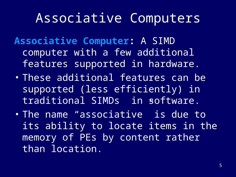
Associative Computer: A SIMD computer with a few additional features supported in hardware.

• These additional features can be supported (less efficiently) in traditional SIMDs in software.

• The name “associative” is due to its ability to locate items in the memory of PEs by content rather than location.

6

Associative Models

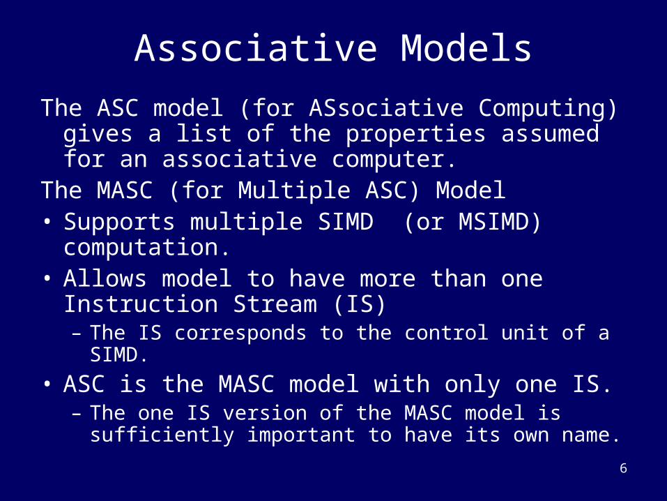
The ASC model (for ASsociative Computing) gives a list of the properties assumed for an associative computer.

The MASC (for Multiple ASC) Model• Supports multiple SIMD (or MSIMD)

computation. • Allows model to have more than one Instruction

Stream (IS)– The IS corresponds to the control unit of a SIMD.

• ASC is the MASC model with only one IS. – The one IS version of the MASC model is sufficiently

important to have its own name.

7

ASC & MASC are KSU Models• Several professors and their graduate students at Kent

State University have worked on models • The STARAN and the ASPRO fully support the ASC

model in hardware. The MPP can easily support ASC but not in hardware.– Prof. Batcher was chief architect or consultant

• Dr. Potter developed a language for ASC• Dr. Baker works on algorithms for models and

architectures to support models• Dr. Walker and his students have investigated a

hardware design to support the ASC and MASC models. • Dr. Batcher and Dr. Potter are currently not actively

working on ASC/MASC models but still provide advice.

8

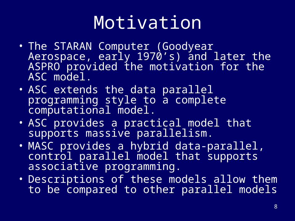
Motivation• The STARAN Computer (Goodyear Aerospace,

early 1970’s) and later the ASPRO provided the motivation for the ASC model.

• ASC extends the data parallel programming style to a complete computational model.

• ASC provides a practical model that supports massive parallelism.

• MASC provides a hybrid data-parallel, control parallel model that supports associative programming.

• Descriptions of these models allow them to be compared to other parallel models

9

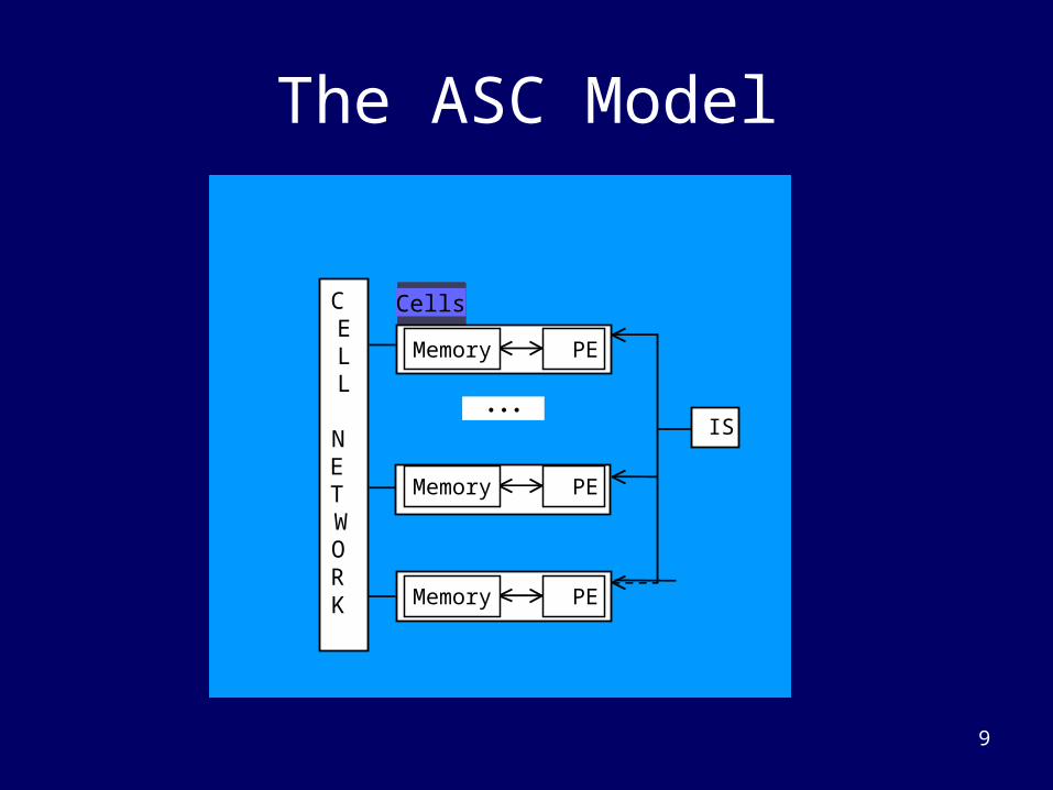
The ASC Model

IS

CELL

NETWORK

PEMemory

Cells

PEMemory

PEMemory

10

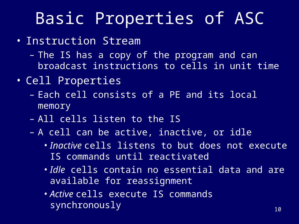
Basic Properties of ASC• Instruction Stream

– The IS has a copy of the program and can broadcast instructions to cells in unit time

• Cell Properties– Each cell consists of a PE and its local memory– All cells listen to the IS – A cell can be active, inactive, or idle

• Inactive cells listens to but does not execute IS commands until reactivated

• Idle cells contain no essential data and are available for reassignment

• Active cells execute IS commands synchronously

11

Basic Properties of ASC

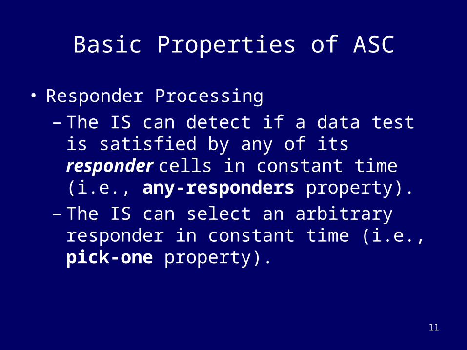
• Responder Processing– The IS can detect if a data test is satisfied by

any of its responder cells in constant time (i.e., any-responders property).

– The IS can select an arbitrary responder in constant time (i.e., pick-one property).

12

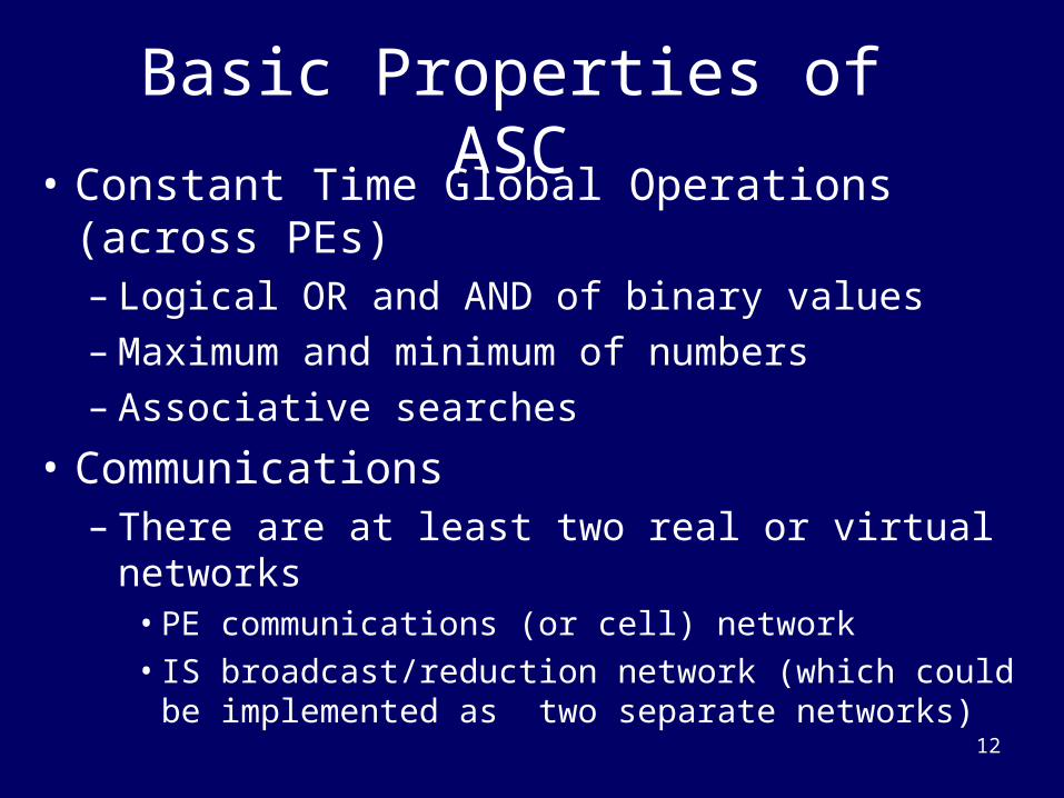
• Constant Time Global Operations (across PEs)– Logical OR and AND of binary values– Maximum and minimum of numbers– Associative searches

• Communications– There are at least two real or virtual networks

• PE communications (or cell) network • IS broadcast/reduction network (which could be

implemented as two separate networks)

Basic Properties of ASC

13

Basic Properties of ASC

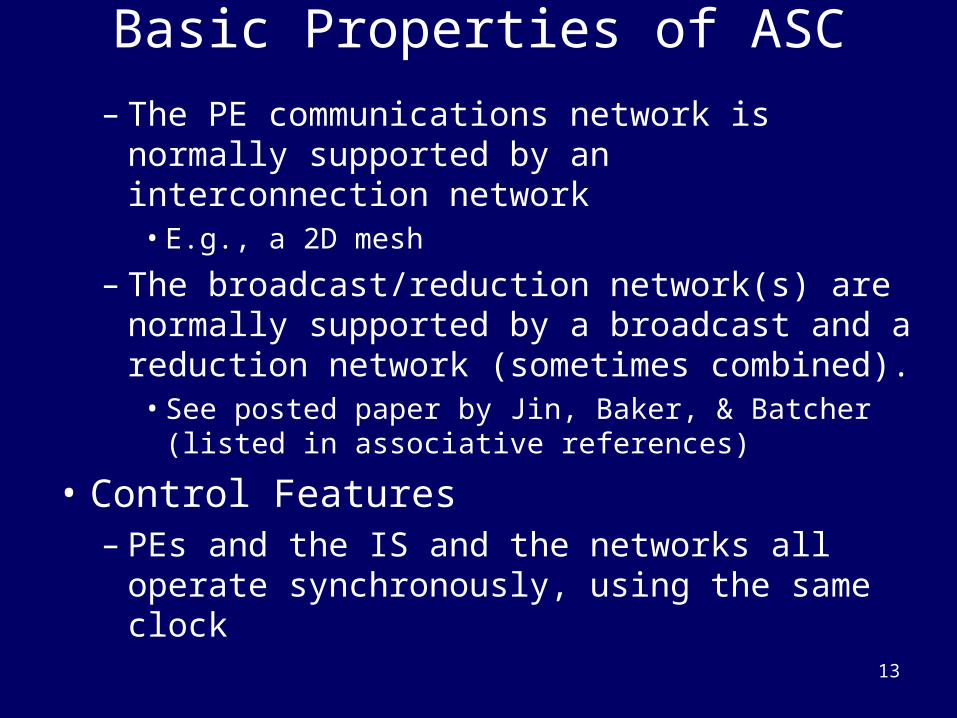
– The PE communications network is normally supported by an interconnection network

• E.g., a 2D mesh

– The broadcast/reduction network(s) are normally supported by a broadcast and a reduction network (sometimes combined).

• See posted paper by Jin, Baker, & Batcher (listed in associative references)

• Control Features– PEs and the IS and the networks all operate

synchronously, using the same clock

14

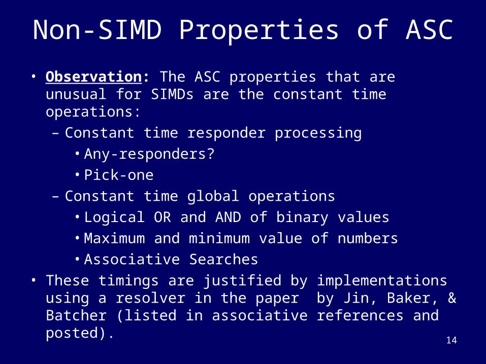
Non-SIMD Properties of ASC

• Observation: The ASC properties that are unusual for SIMDs are the constant time operations:– Constant time responder processing

• Any-responders?• Pick-one

– Constant time global operations• Logical OR and AND of binary values• Maximum and minimum value of numbers• Associative Searches

• These timings are justified by implementations using a resolver in the paper by Jin, Baker, & Batcher (listed in associative references and posted).

15

1

Busy-idle

Dodge

Ford

Ford

Make

Subaru

Color

PE1

PE2

PE3

PE4

PE5

PE6

PE7

red

blue

white

red

Year

1994

1996

1998

1997

Model PriceOnlot

1

1

0

0

0

0

1

0

1

1

0

0

1

IS

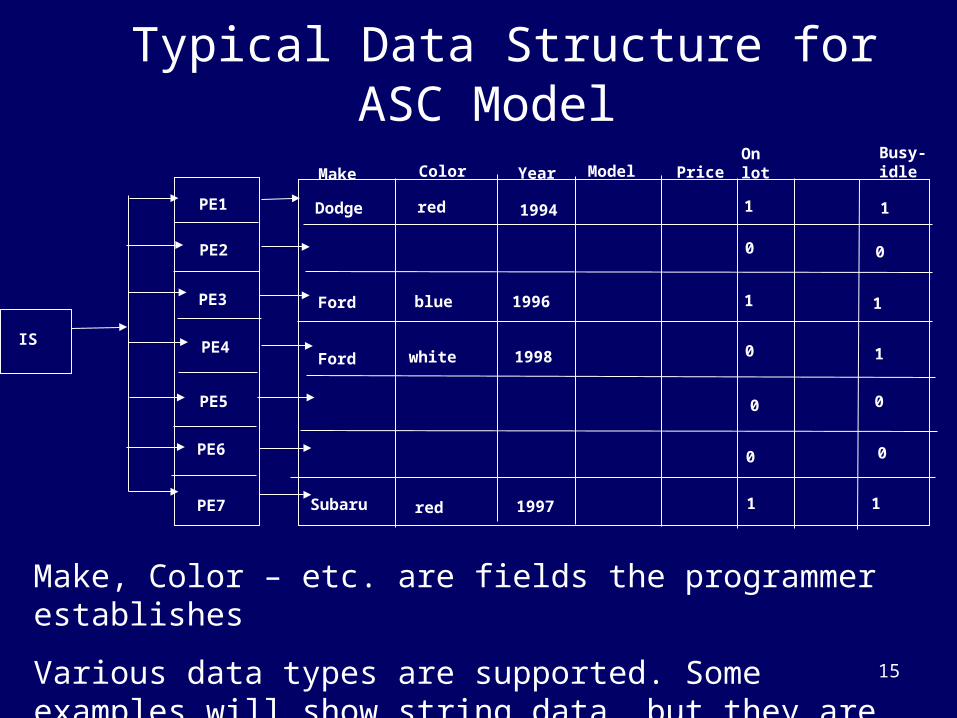
Typical Data Structure for ASC Model

Make, Color – etc. are fields the programmer establishes

Various data types are supported. Some examples will show string data, but they are not supported in the ASC simulator.

16

Dodge

Ford

Ford

Make

Subaru

Color

PE1

PE2

PE3

PE4

PE5

PE6

PE7

red

blue

white

red

Year

1994

1996

1998

1997

Model PriceOnlot

1

1

0

0

0

0

1

Busy-idle

1

0

1

1

0

0

1

IS

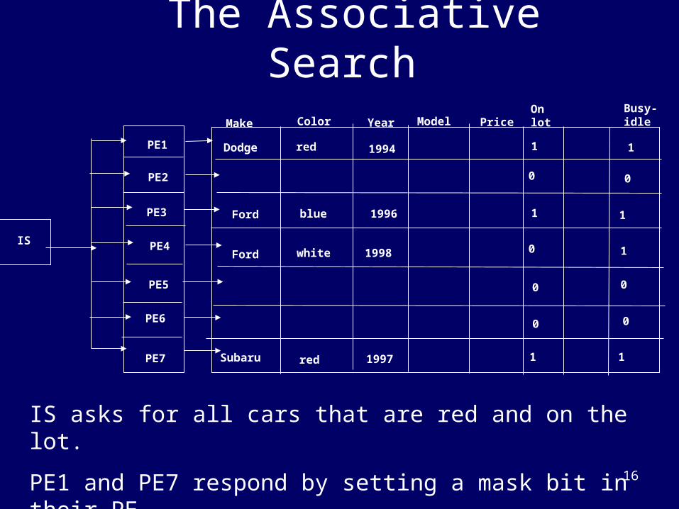
The Associative Search

IS asks for all cars that are red and on the lot.

PE1 and PE7 respond by setting a mask bit in their PE.

17

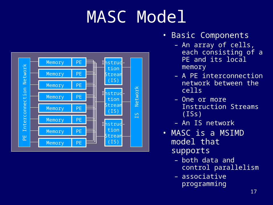
MASC Model• Basic Components

– An array of cells, each consisting of a PE and its local memory

– A PE interconnection network between the cells

– One or more Instruction Streams (ISs)

– An IS network

• MASC is a MSIMD model that supports – both data and control

parallelism– associative

programming

Memory

Memory

Memory

Memory

Memory

Memory

Memory

Memory

PE

Inte

rcon

nect

ion

Net

wor

k

IS N

etw

ork

PE

PE

PE

PE

PE

PE

PE

PE

Instruc-tion

Stream(IS)

Instruc-tion

Stream(IS)

Instruc-tion

Stream(IS)

18

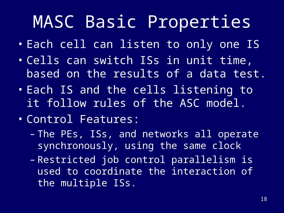
MASC Basic Properties• Each cell can listen to only one IS

• Cells can switch ISs in unit time, based on the results of a data test.

• Each IS and the cells listening to it follow rules of the ASC model.

• Control Features:– The PEs, ISs, and networks all operate

synchronously, using the same clock– Restricted job control parallelism is used to

coordinate the interaction of the multiple ISs.

19

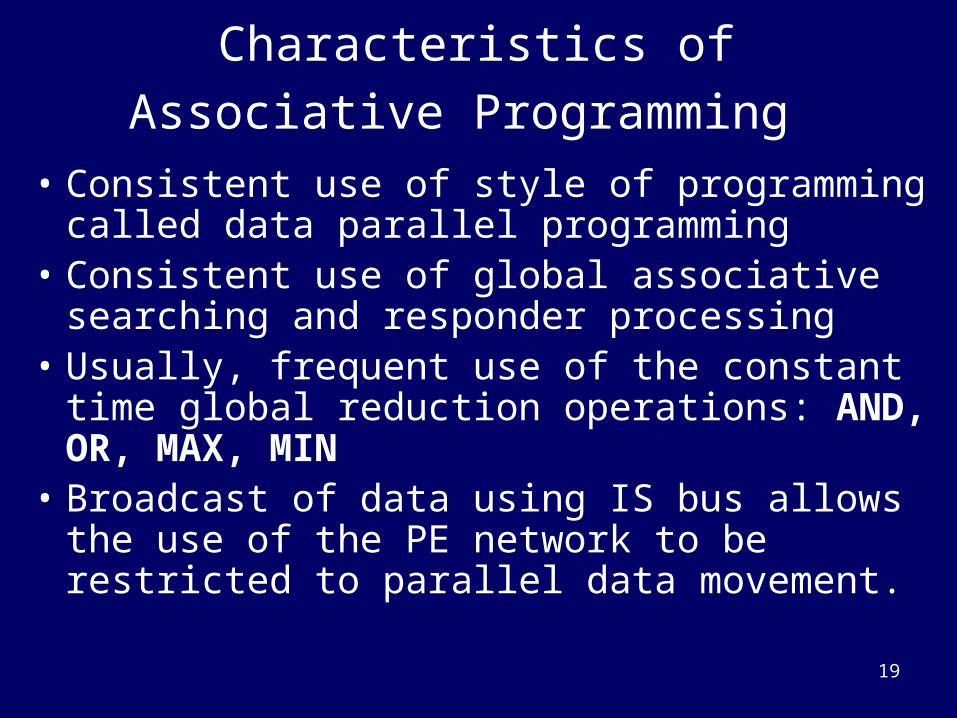
Characteristics of Associative

Programming • Consistent use of style of programming called

data parallel programming• Consistent use of global associative searching

and responder processing• Usually, frequent use of the constant time global

reduction operations: AND, OR, MAX, MIN• Broadcast of data using IS bus allows the use of

the PE network to be restricted to parallel data movement.

20

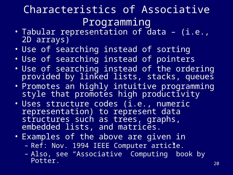
Characteristics of Associative Programming

• Tabular representation of data – (i.e., 2D arrays)• Use of searching instead of sorting• Use of searching instead of pointers• Use of searching instead of the ordering provided

by linked lists, stacks, queues• Promotes an highly intuitive programming style

that promotes high productivity• Uses structure codes (i.e., numeric

representation) to represent data structures such as trees, graphs, embedded lists, and matrices.

• Examples of the above are given in– Ref: Nov. 1994 IEEE Computer article.– Also, see “Associative Computing” book by Potter.

21

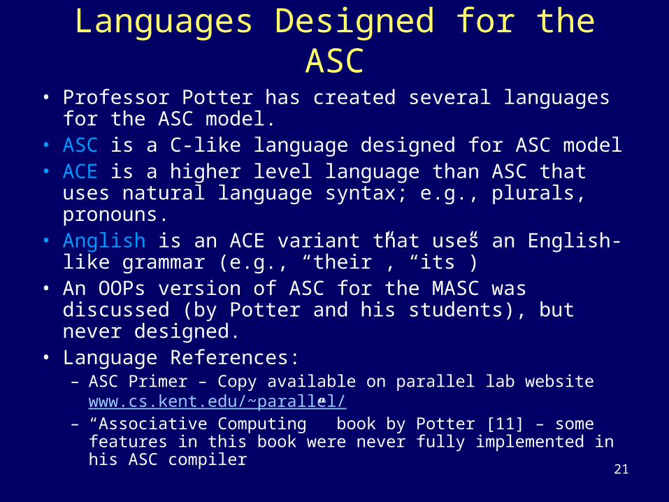
Languages Designed for the ASC

• Professor Potter has created several languages for the ASC model.

• ASC is a C-like language designed for ASC model• ACE is a higher level language than ASC that uses

natural language syntax; e.g., plurals, pronouns.• Anglish is an ACE variant that uses an English-like

grammar (e.g., “their”, “its”) • An OOPs version of ASC for the MASC was discussed

(by Potter and his students), but never designed.• Language References:

– ASC Primer – Copy available on parallel lab website www.cs.kent.edu/~parallel/

– “Associative Computing” book by Potter [11] – some features in this book were never fully implemented in his ASC compiler

22

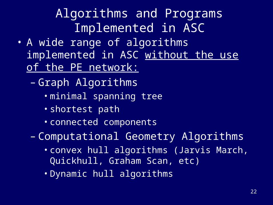
Algorithms and Programs Implemented in ASC

• A wide range of algorithms implemented in ASC without the use of the PE network:– Graph Algorithms

• minimal spanning tree• shortest path• connected components

– Computational Geometry Algorithms• convex hull algorithms (Jarvis March, Quickhull,

Graham Scan, etc)• Dynamic hull algorithms

23

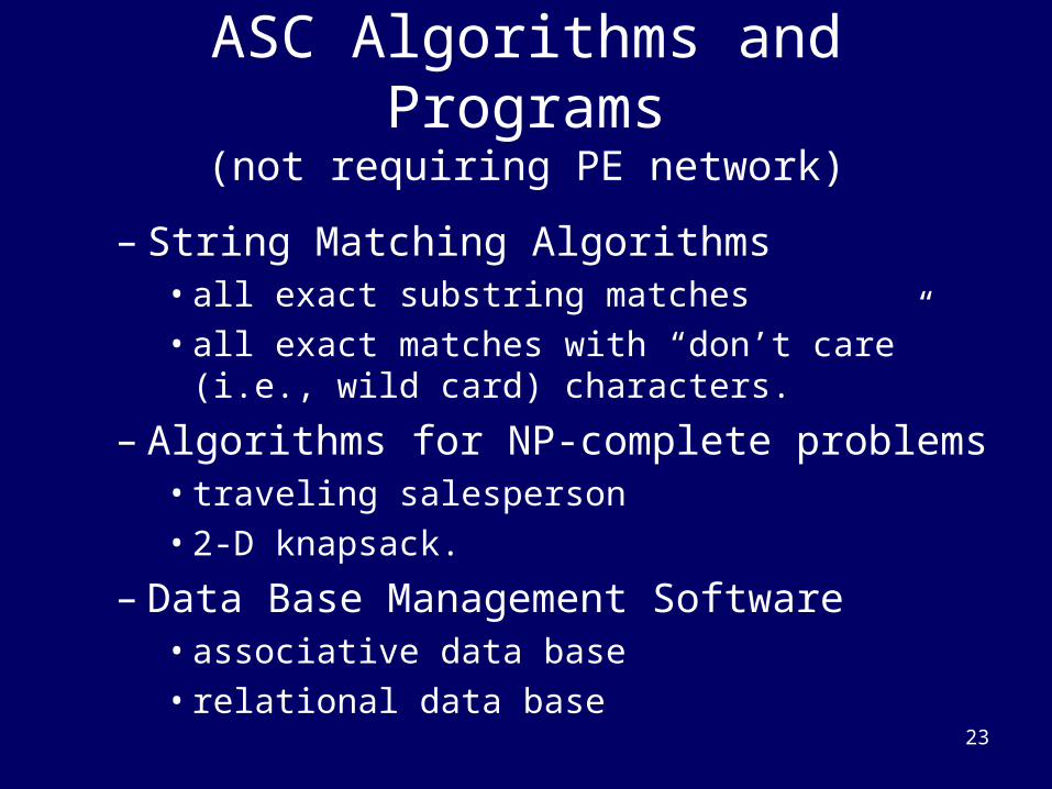
ASC Algorithms and Programs(not requiring PE network)

– String Matching Algorithms• all exact substring matches• all exact matches with “don’t care” (i.e., wild card)

characters.

– Algorithms for NP-complete problems• traveling salesperson • 2-D knapsack.

– Data Base Management Software• associative data base• relational data base

24

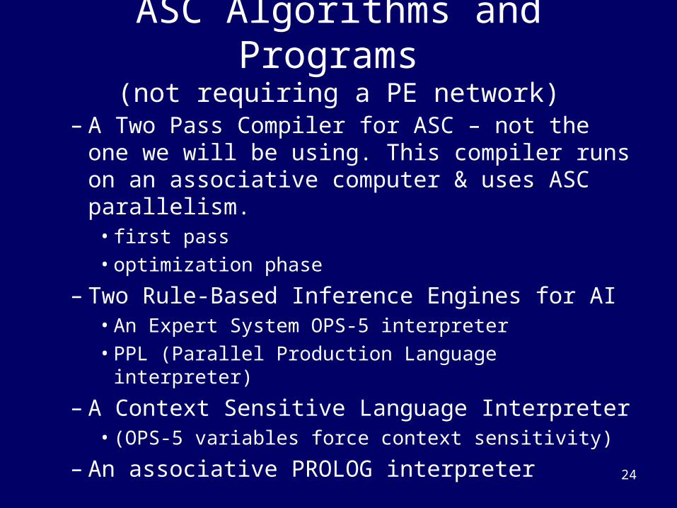
ASC Algorithms and Programs (not requiring a PE network)

– A Two Pass Compiler for ASC – not the one we will be using. This compiler runs on an associative computer & uses ASC parallelism.

• first pass• optimization phase

– Two Rule-Based Inference Engines for AI• An Expert System OPS-5 interpreter• PPL (Parallel Production Language interpreter)

– A Context Sensitive Language Interpreter• (OPS-5 variables force context sensitivity)

– An associative PROLOG interpreter

25

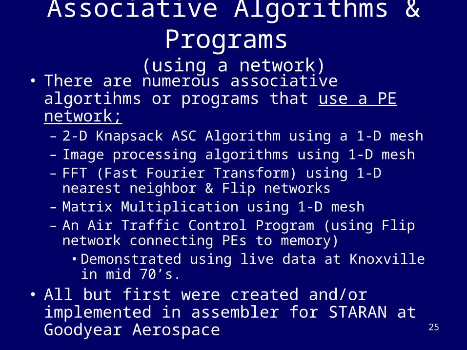
Associative Algorithms & Programs

(using a network)• There are numerous associative algortihms or

programs that use a PE network;– 2-D Knapsack ASC Algorithm using a 1-D mesh– Image processing algorithms using 1-D mesh– FFT (Fast Fourier Transform) using 1-D nearest

neighbor & Flip networks– Matrix Multiplication using 1-D mesh– An Air Traffic Control Program (using Flip network

connecting PEs to memory)• Demonstrated using live data at Knoxville in mid

70’s.

• All but first were created and/or implemented in assembler for STARAN at Goodyear Aerospace

26

Example 1 - MST

• A graph has nodes labeled by some identifying letter or number and arcs which are directional and have weights associated with them.

• Such a graph could represent a map where the nodes are cities and the arc weights give the mileage between two cities.

A B

C D

E

3

5 2

54

27

The MST Problem

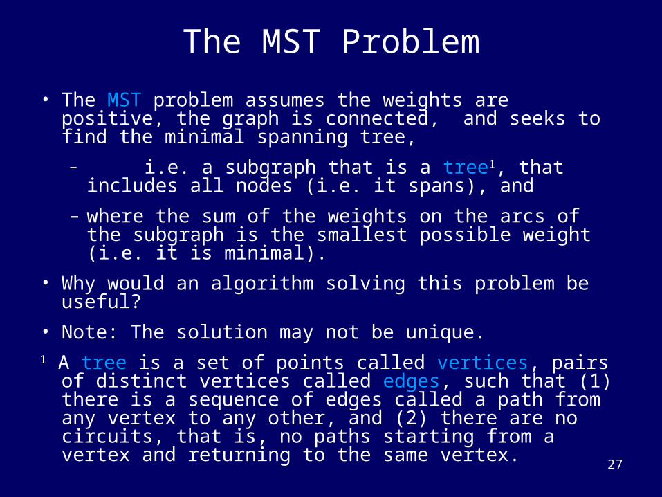
• The MST problem assumes the weights are positive, the graph is connected, and seeks to find the minimal spanning tree,

– i.e. a subgraph that is a tree1, that includes all nodes (i.e. it spans), and

– where the sum of the weights on the arcs of the subgraph is the smallest possible weight (i.e. it is minimal).

• Why would an algorithm solving this problem be useful?

• Note: The solution may not be unique.1 A tree is a set of points called vertices, pairs of distinct

vertices called edges, such that (1) there is a sequence of edges called a path from any vertex to any other, and (2) there are no circuits, that is, no paths starting from a vertex and returning to the same vertex.

28

An Example

DE

HI

F CG

BA

86

53

3

2

2

2

1

6

1

4

2

47

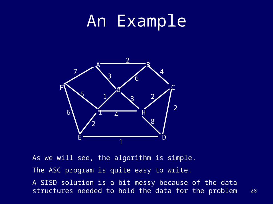
As we will see, the algorithm is simple.

The ASC program is quite easy to write.

A SISD solution is a bit messy because of the data structures needed to hold the data for the problem

29

An Example – Step 0

DE

HI

F CG

BA

86

53

3

2

2

2

1

6

1

4

2

47

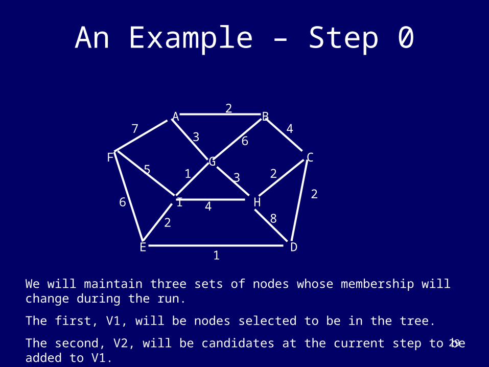
We will maintain three sets of nodes whose membership will change during the run.

The first, V1, will be nodes selected to be in the tree.

The second, V2, will be candidates at the current step to be added to V1.

The third, V3, will be nodes not considered yet.

30

An Example – Step 0

DE

HI

F CG

BA

86

53

3

2

2

2

1

6

1

4

2

47

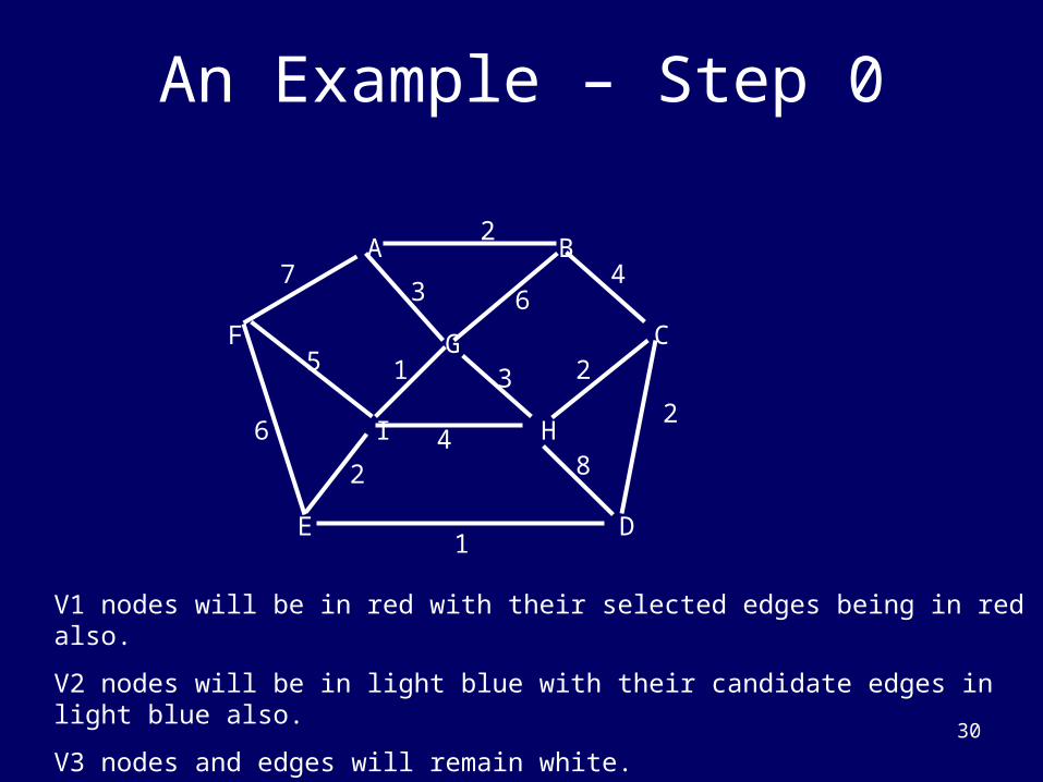
V1 nodes will be in red with their selected edges being in red also.

V2 nodes will be in light blue with their candidate edges in light blue also.

V3 nodes and edges will remain white.

31

An Example – Step 1

DE

HI

F CG

BA

86

53

3

2

2

2

1

6

1

4

2

47

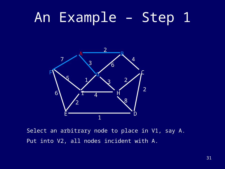
Select an arbitrary node to place in V1, say A.

Put into V2, all nodes incident with A.

32

An Example – Step 2

DE

HI

F CG

BA

86

53

3

2

2

2

1

6

1

4

2

47

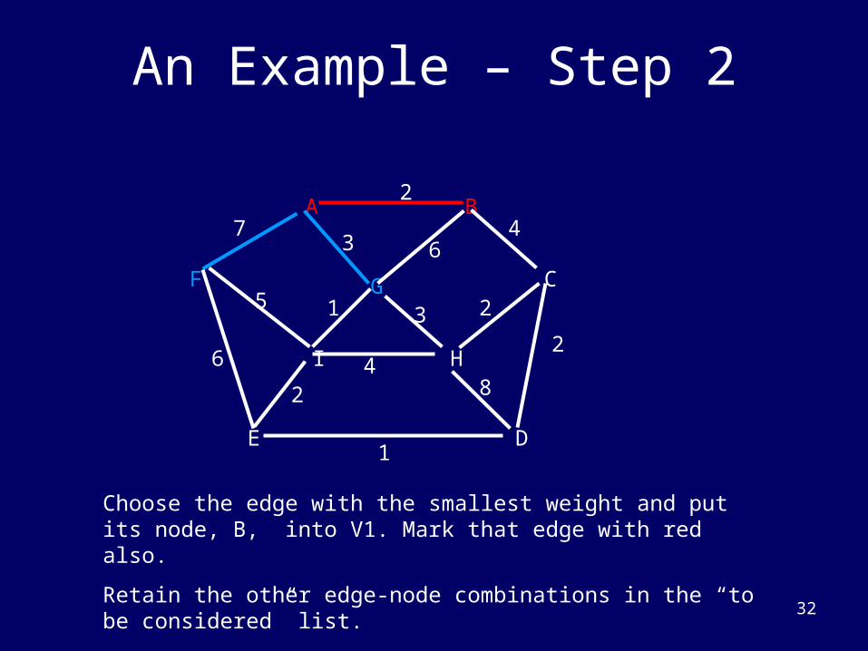
Choose the edge with the smallest weight and put its node, B, into V1. Mark that edge with red also.

Retain the other edge-node combinations in the “to be considered” list.

33

An Example – Step 3

DE

HI

F CG

BA

86

53

3

2

2

2

1

6

1

4

2

47

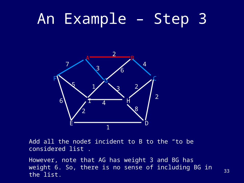
Add all the nodes incident to B to the “to be considered list”.

However, note that AG has weight 3 and BG has weight 6. So, there is no sense of including BG in the list.

34

An Example – Step 4

DE

HI

F CG

BA

86

53

3

2

2

2

1

6

1

4

2

47

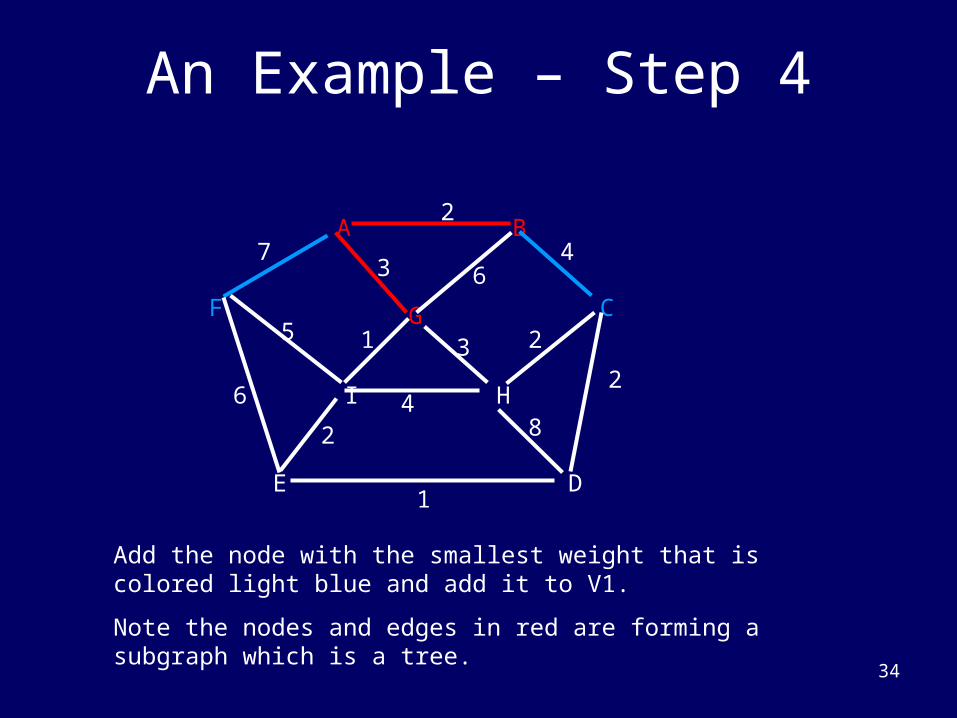
Add the node with the smallest weight that is colored light blue and add it to V1.

Note the nodes and edges in red are forming a subgraph which is a tree.

35

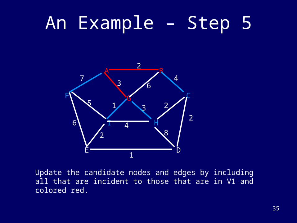
An Example – Step 5

DE

HI

F CG

BA

86

53

3

2

2

2

1

6

1

4

2

47

Update the candidate nodes and edges by including all that are incident to those that are in V1 and colored red.

36

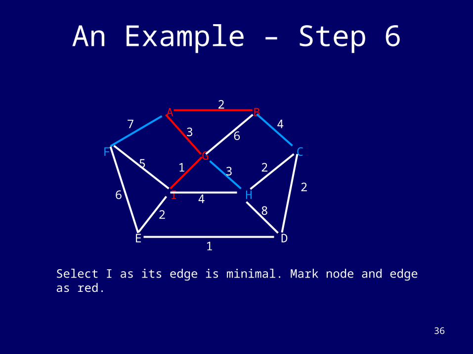
An Example – Step 6

DE

HI

F CG

BA

86

53

3

2

2

2

1

6

1

4

2

47

Select I as its edge is minimal. Mark node and edge as red.

37

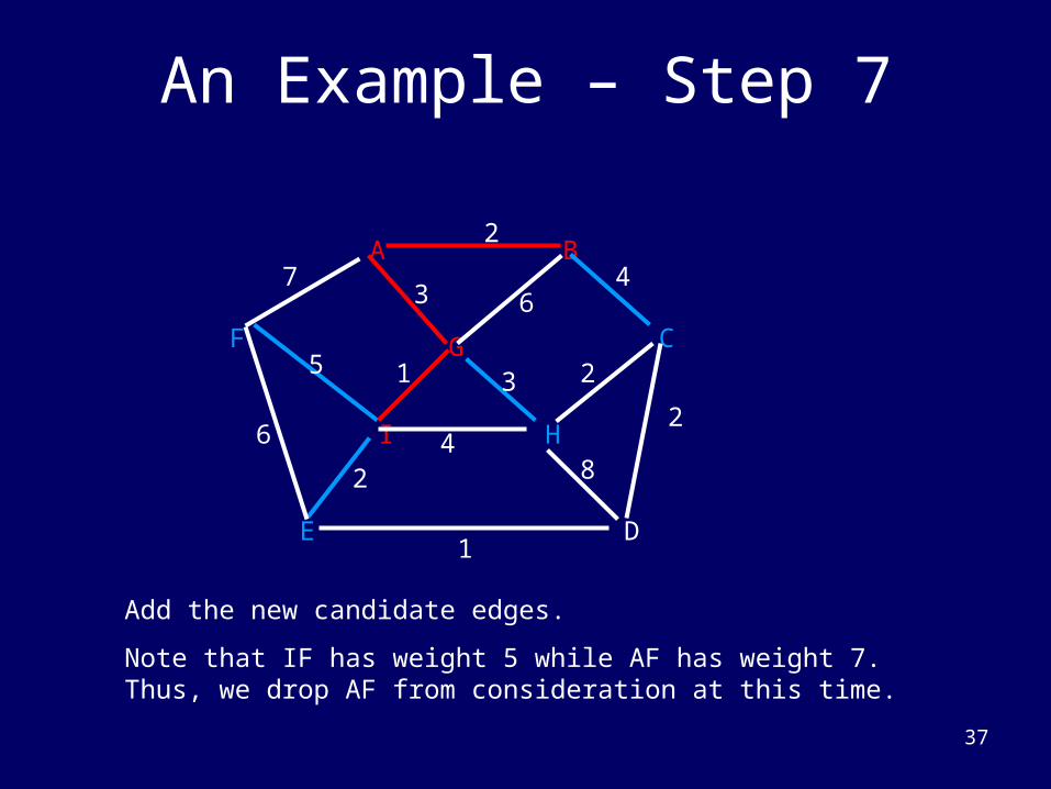
An Example – Step 7

DE

HI

F CG

BA

86

53

3

2

2

2

1

6

1

4

2

47

Add the new candidate edges.

Note that IF has weight 5 while AF has weight 7. Thus, we drop AF from consideration at this time.

38

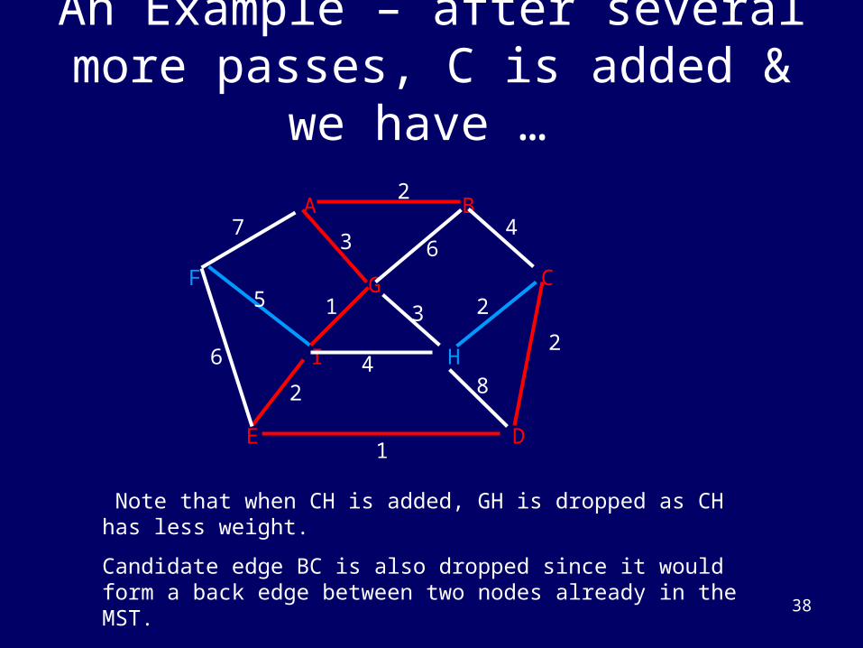
An Example – after several more passes, C is added & we have …

DE

HI

F CG

BA

86

53

3

2

2

2

1

6

1

4

2

47

Note that when CH is added, GH is dropped as CH has less weight.

Candidate edge BC is also dropped since it would form a back edge between two nodes already in the MST.

When there are no more nodes to be considered, i.e. no more in V3, we obtain the final solution.

39

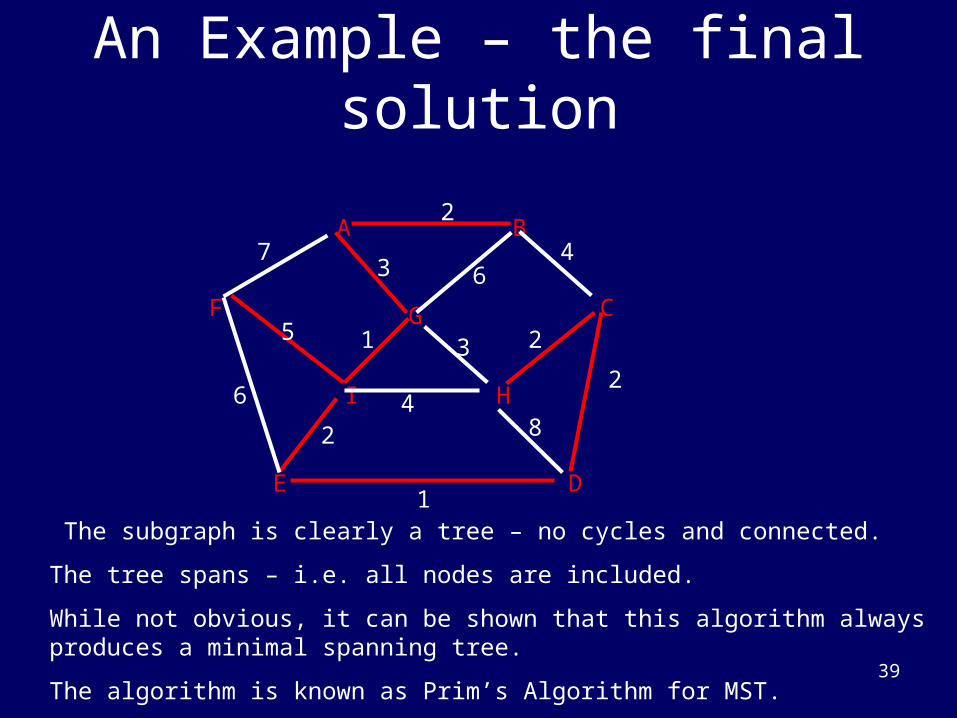
An Example – the final solution

DE

HI

F CG

BA

86

53

3

2

2

2

1

6

1

4

2

47

The subgraph is clearly a tree – no cycles and connected.

The tree spans – i.e. all nodes are included.

While not obvious, it can be shown that this algorithm always produces a minimal spanning tree.

The algorithm is known as Prim’s Algorithm for MST.

40

The ASC Program vs a SISD solution in , say, C, C++, or Java

• First, think about how you would write the program in C or C++.

• The usual solution uses some way of maintaining the sets as lists using pointers or references. – See solutions to MST in Algorithms texts by Baase in the posted

references.• In the ASC language, pointers are not even supported as

they are not needed and their use is likely to result in inefficient SIMD algorithms

• An ASC algorithm will be developed for Prim’s sequential algorithm using a pseudocode that is based on the ASC language.

• The ASC language user’s guide is posted at www.cs.kent.edu/~parallel/, but its use is not required.

• The ASC algorithm can be used to create a program in ASC for the ASC simulator or in Cn for ClearSpeed.

41

ASC-MST Algorithm Preliminaries

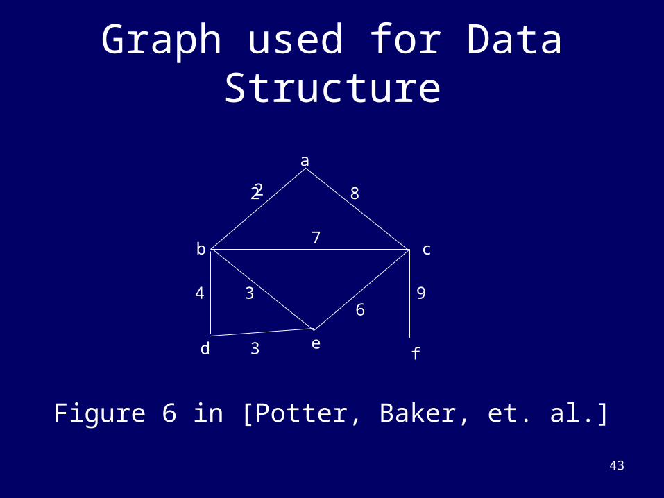
• Next, a “data structure” level presentation of Prim’s algorithm for the MST is given.

• The data structure used is illustrated in the next two slides. – This example is from the Nov. 1994 IEEE Computer

paper cited in the references.

• There are two types of variables for the ASC model, namely– the parallel variables (i.e., ones for the PEs) – the scalar variables (ie., the ones used by the IS). – Scalar variables are essentially global variables.

• Could replace each scalar variable with its scalar value stored in each entry of a parallel variable.

42

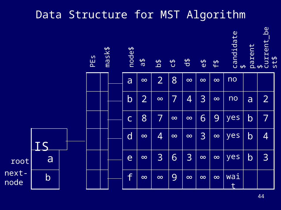
ASC-MST Algorithm Preliminaries (cont.)

• In order to distinguish between variable types here, the parallel variables names will end with a “$” symbol.

• Each step in this algorithm takes constant time. • One MST edge is selected during each pass through the

loop in this algorithm.• Since a spanning tree has n-1 edges, the running time of

this algorithm is O(n) and its cost is O(n 2).– Definition of cost is (running time) (number of processors)

• Since the sequential running time of the Prim MST algorithm is O(n 2) and is time optimal, this parallel implementation is cost optimal.– Cost & optimality will be covered in parallel algorithm

performance evaluation chapter (See Ch 7 of Quinn)

43

Graph used for Data Structure

Figure 6 in [Potter, Baker, et. al.]

a

b c

d ef

2 8

96

3

3

4

7

2

44

Data Structure for MST Algorithm

curr

ent_

best

$

cand

idat

e$

next-node b

a

IS

wait∞∞∞9∞∞f

3byes∞∞363∞e

4byes∞3∞∞4∞d

7byes96∞∞78 c

2ano∞347∞2b

no∞∞∞82∞aP

Es

mas

k$

node

$

a$ b$ pare

nt$

rootc$ d$ e$ f$

45

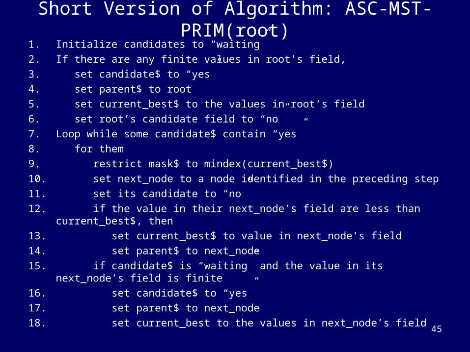
Short Version of Algorithm: ASC-MST-PRIM(root)1. Initialize candidates to “waiting”

2. If there are any finite values in root’s field,

3. set candidate$ to “yes”

4. set parent$ to root

5. set current_best$ to the values in root’s field

6. set root’s candidate field to “no”

7. Loop while some candidate$ contain “yes”

8. for them

9. restrict mask$ to mindex(current_best$)

10. set next_node to a node identified in the preceding step

11. set its candidate to “no”

12. if the value in their next_node’s field are less than current_best$, then

13. set current_best$ to value in next_node’s field

14. set parent$ to next_node

15. if candidate$ is “waiting” and the value in its next_node’s field is finite

16. set candidate$ to “yes”

17. set parent$ to next_node

18. set current_best to the values in next_node’s field

46

Comments on ASC-MST Algorithm• The three preceding slides are Figure 6 in [Potter, Baker,

et.al.] IEEE Computer, Nov 1994].• Preceding slide gives a compact, data-structures level

pseudo-code description for this algorithm – Pseudo-code illustrates Potter’s use of pronouns

(e.g., them, its) and possessive nouns.– The mindex function returns the index of a processor

holding the minimal value.– This MST pseudo-code is much shorter and simpler

than data-structure level sequential MST pseudo-codes

• e.g., see one of Baase’s textbooks cited in references• Algorithm given in Baase’s books is identical to this parallel

algorithm, except for a sequential computer

• Next, a more detailed explanation of the algorithm in preceding slide will be given next.

47

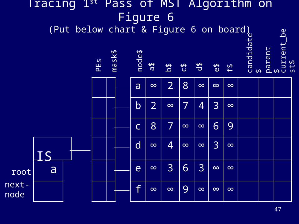
Tracing 1st Pass of MST Algorithm on Figure 6 (Put below chart & Figure 6 on board)

curr

ent_

best

$

cand

idat

e$

next-node

a

IS

∞∞∞9∞∞f

∞∞363∞e

∞3∞∞4∞d

96∞∞78 c

∞347∞2b

∞∞∞82∞aP

Es

mas

k$

node

$

a$ b$ pare

nt$

rootc$ d$ e$ f$

48

Algorithm: ASC-MST-PRIM• Initially assign any node to root.• All processors set

– candidate$ to “wait”– current-best$ to – the candidate field for the root node to “no”

• All processors whose distance d from their node to root node is finite do– Set their candidate$ field to “yes– Set their parent$ field to root.– Set current_best$ = d.

49

Algorithm: ASC-MST-PRIM (cont. 2/3)

• While the candidate field of some processor is “yes”, – Restrict the active processors to those whose

candidate field is “yes” and (for these processors) do• Compute the minimum value x of current_best$.• Restrict the active processors to those with

current_best$ = x and do– pick an active processor, say node y.

» Set the candidate$ value of node y to “no” – Set the scalar variable next-node to y.

50

Algorithm: ASC-MST-PRIM (cont. 3/3)

–If the value z in the next_node column of a processor is less than its current_best$ value, then

»Set current_best$ to z. »Set parent$ to next_node

– For all processors, if candidate$ is “waiting” and the distance of its node from next_node y is finite, then

• Set candidate$ to “yes”• Set current_best$ to the distance of its node from

y.• Set parent$ to y

51

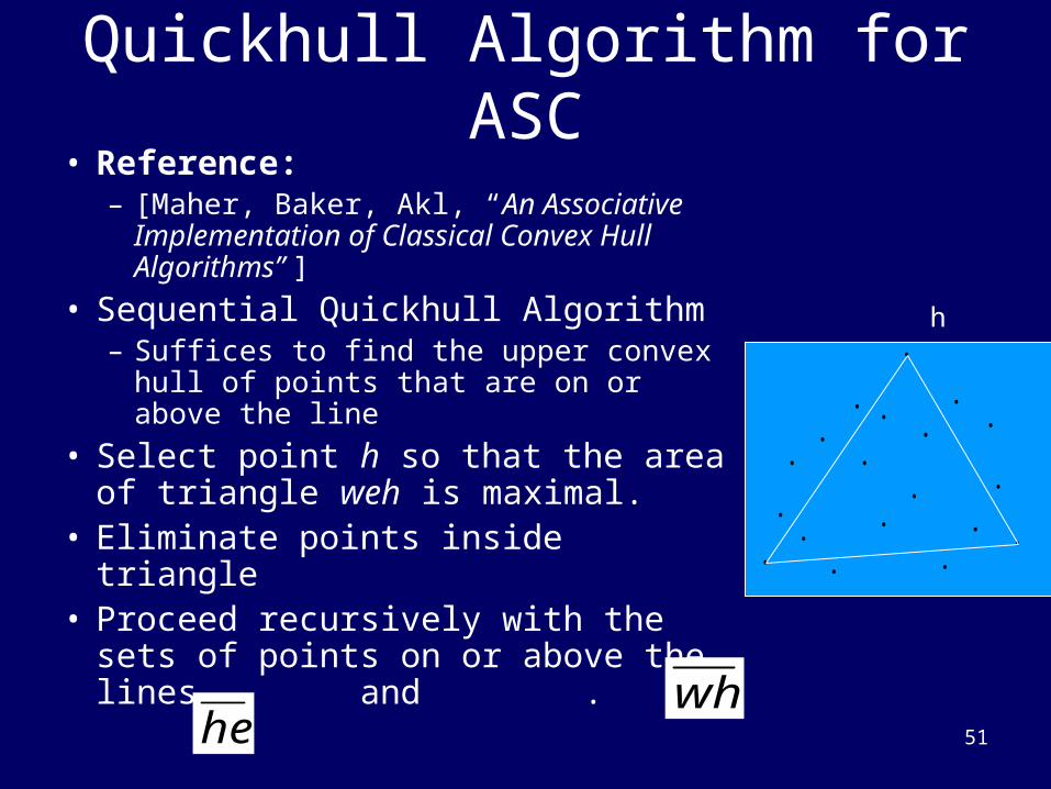
Quickhull Algorithm for ASC• Reference:

– [Maher, Baker, Akl, “An Associative Implementation of Classical Convex Hull Algorithms” ]

• Sequential Quickhull Algorithm– Suffices to find the upper convex hull

of points that are on or above the line

• Select point h so that the area of triangle weh is maximal.

• Eliminate points inside triangle• Proceed recursively with the sets

of points on or above the lines and .

whhe

we

h

52

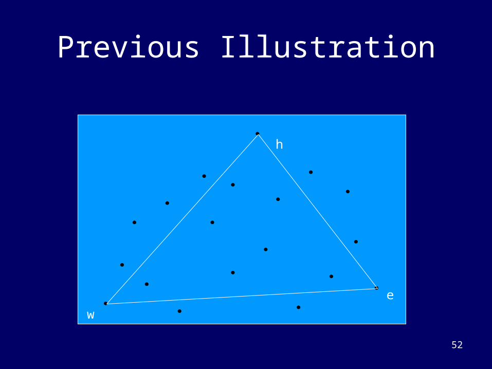
Previous Illustration

w

e

h

53

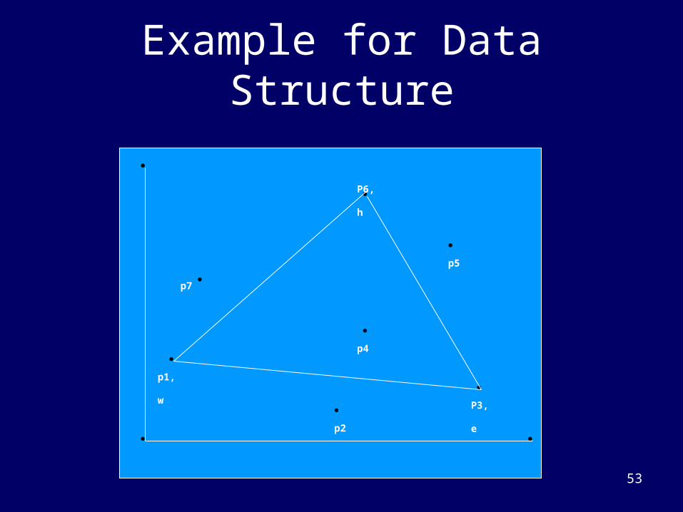
Example for Data Structure

p1, w

p7

p2

P3, e

p4

p5

P6, h

54

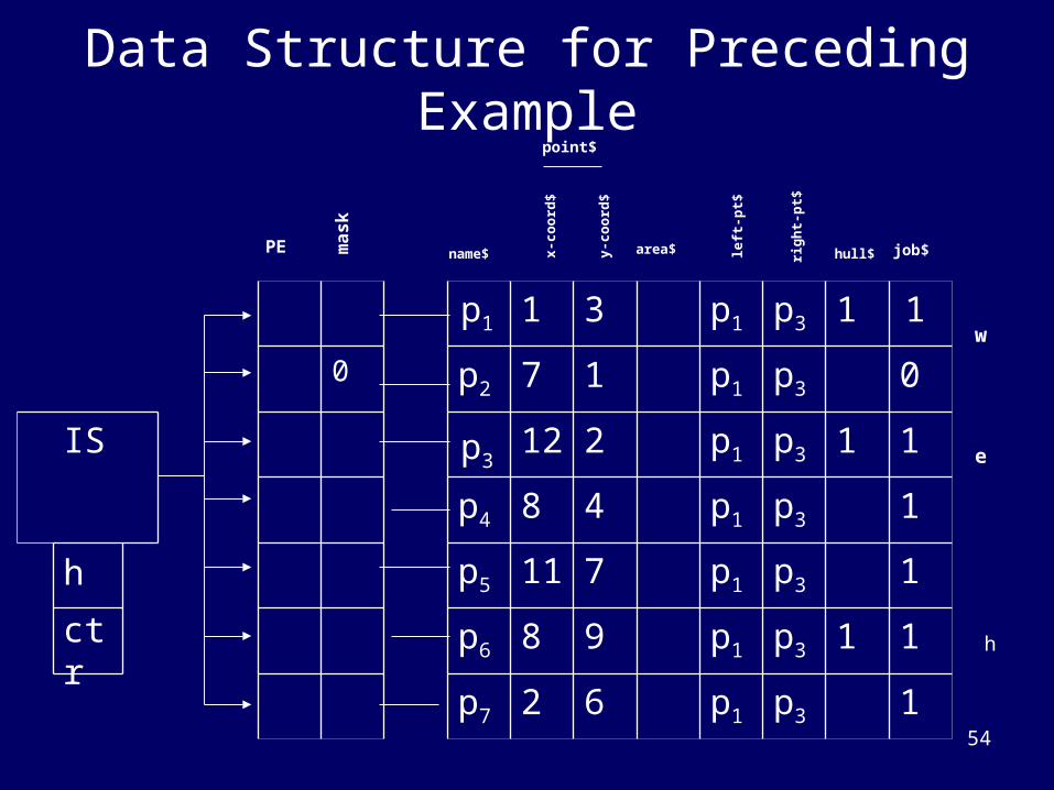
Data Structure for Preceding Example

1p3p162p7

11p3p198p6ctr

1p3p1711p5h

1p3p148p4

11p3p1212IS

0p3p117p20

11p3p131p1

job$hull$righ

t-p

t$

area$name$ left

-pt$

x-co

ord

$

y-co

ord

$

point$

w

ep3

h

PE ma

sk

55

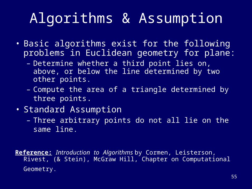
Algorithms & Assumption

• Basic algorithms exist for the following problems in Euclidean geometry for plane:– Determine whether a third point lies on, above, or

below the line determined by two other points.– Compute the area of a triangle determined by three

points.• Standard Assumption

– Three arbitrary points do not all lie on the same line.

Reference: Introduction to Algorithms by Cormen, Leisterson, Rivest,

(& Stein), McGraw Hill, Chapter on Computational Geometry.

56

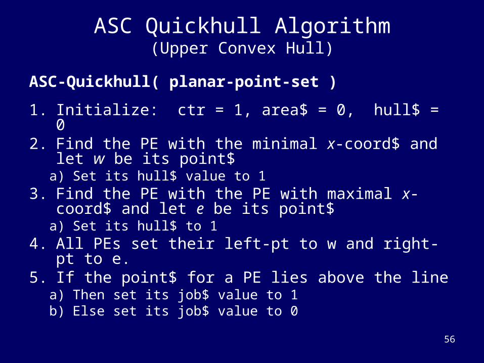
ASC Quickhull Algorithm(Upper Convex Hull)

ASC-Quickhull( planar-point-set )

1. Initialize: ctr = 1, area$ = 0, hull$ = 02. Find the PE with the minimal x-coord$ and let

w be its point$a) Set its hull$ value to 1

3. Find the PE with the PE with maximal x-coord$ and let e be its point$

a) Set its hull$ to 14. All PEs set their left-pt to w and right-pt to e.5. If the point$ for a PE lies above the line

a) Then set its job$ value to 1b) Else set its job$ value to 0

57

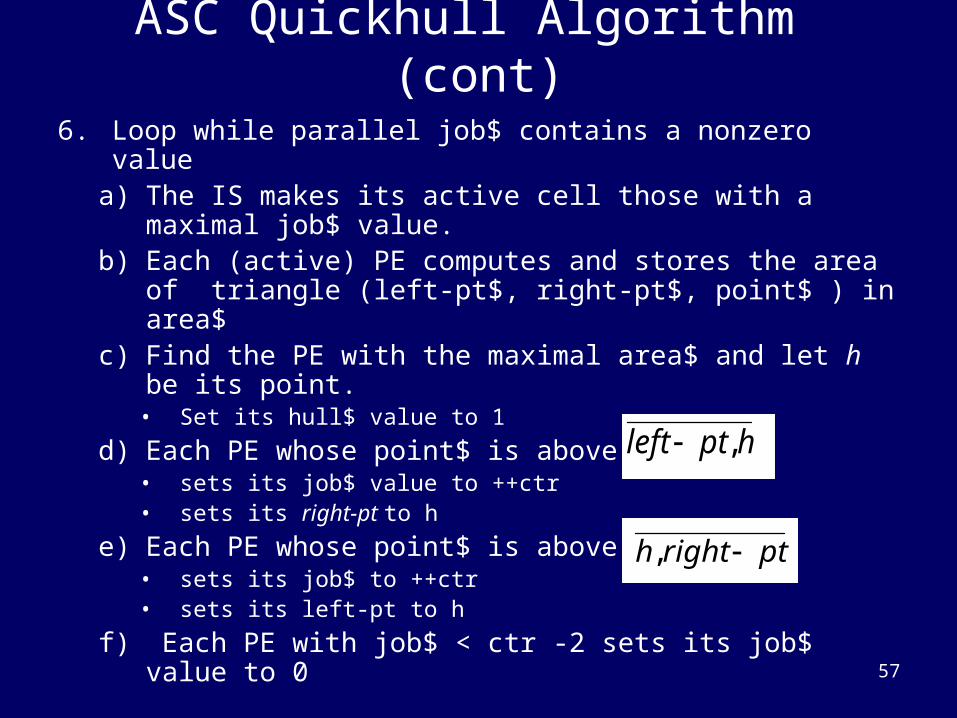
ASC Quickhull Algorithm (cont)

6. Loop while parallel job$ contains a nonzero valuea) The IS makes its active cell those with a maximal

job$ value.b) Each (active) PE computes and stores the area of

triangle (left-pt$, right-pt$, point$ ) in area$c) Find the PE with the maximal area$ and let h be its

point.• Set its hull$ value to 1

d) Each PE whose point$ is above• sets its job$ value to ++ctr• sets its right-pt to h

e) Each PE whose point$ is above• sets its job$ to ++ctr• sets its left-pt to h

f) Each PE with job$ < ctr -2 sets its job$ value to 0

hptleft ,

ptrighth ,

58

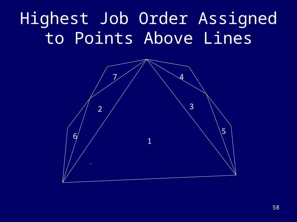
Highest Job Order Assigned to Points Above Lines

1

2

6

7

3

5

4

59

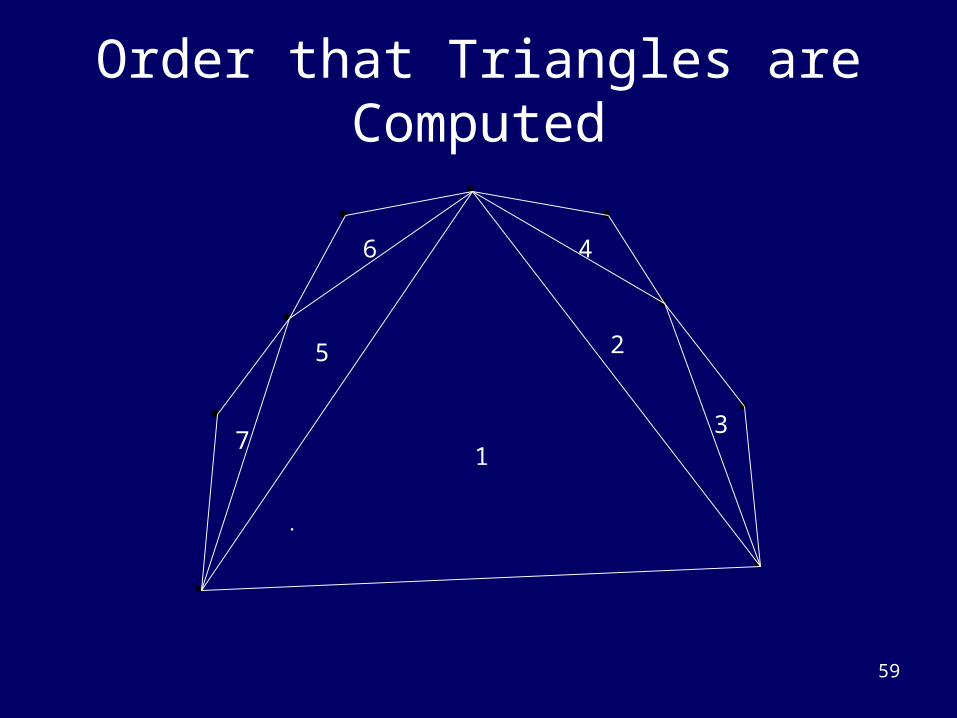
Order that Triangles are Computed

1

5

7

6

2

3

4

60

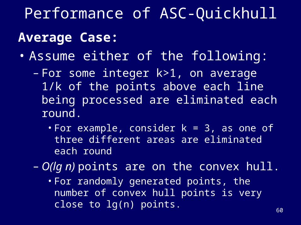
Performance of ASC-Quickhull

Average Case:

• Assume either of the following: – For some integer k>1, on average 1/k of the

points above each line being processed are eliminated each round.

• For example, consider k = 3, as one of three different areas are eliminated each round

– O(lg n) points are on the convex hull.• For randomly generated points, the number of

convex hull points is very close to lg(n) points.

61

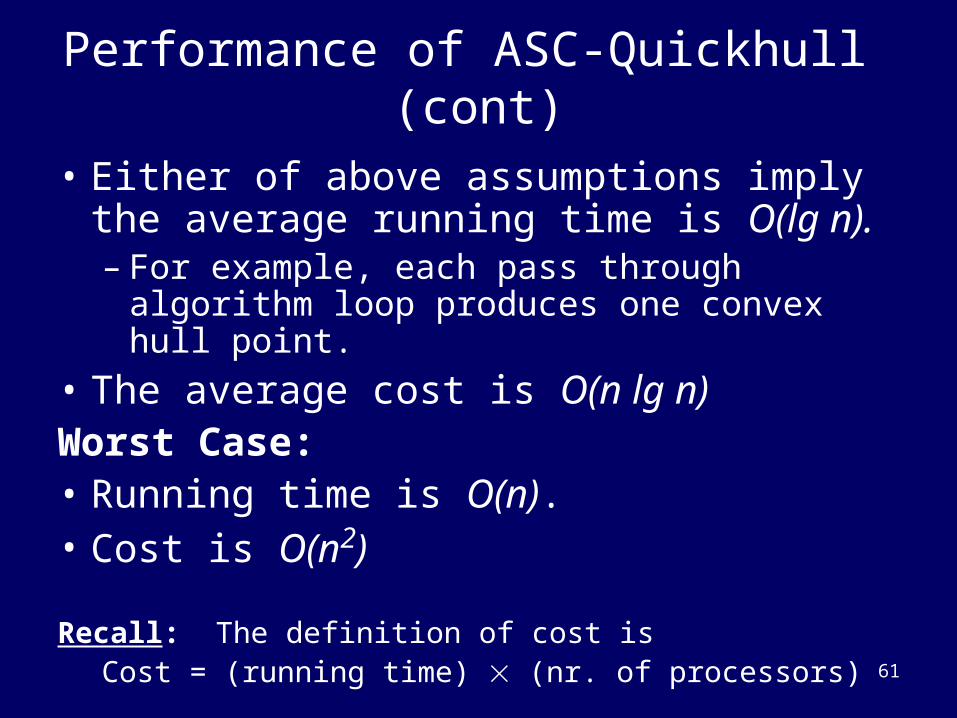
Performance of ASC-Quickhull (cont)

• Either of above assumptions imply the average running time is O(lg n). – For example, each pass through algorithm

loop produces one convex hull point.

• The average cost is O(n lg n)Worst Case:• Running time is O(n).• Cost is O(n2)

Recall: The definition of cost is Cost = (running time) (nr. of processors)

62

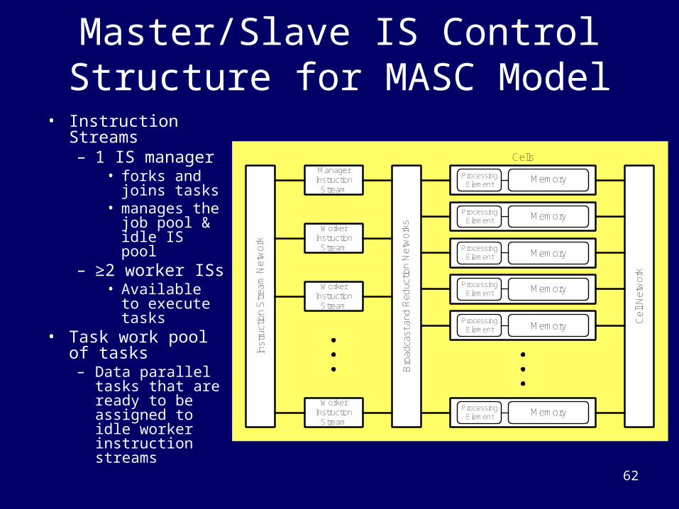
Master/Slave IS Control Structure for MASC Model

• Instruction Streams– 1 IS manager

• forks and joins tasks

• manages the job pool & idle IS pool

– ≥2 worker ISs• Available to

execute tasks

• Task work pool of tasks– Data parallel

tasks that are ready to be assigned to idle worker instruction streams

Inst

ruct

ion

Str

eam

Net

wor

k

Bro

adca

st a

nd R

educ

tion

Net

wor

ks

Cel

l Net

wor

k

ManagerInstruction

Stream

WorkerInstruction

Stream

WorkerInstruction

Stream

WorkerInstruction

Stream

Cells

MemoryProcessingElement

ProcessingElement

ProcessingElement

ProcessingElement

ProcessingElement

ProcessingElement

Memory

Memory

Memory

Memory

Memory

63

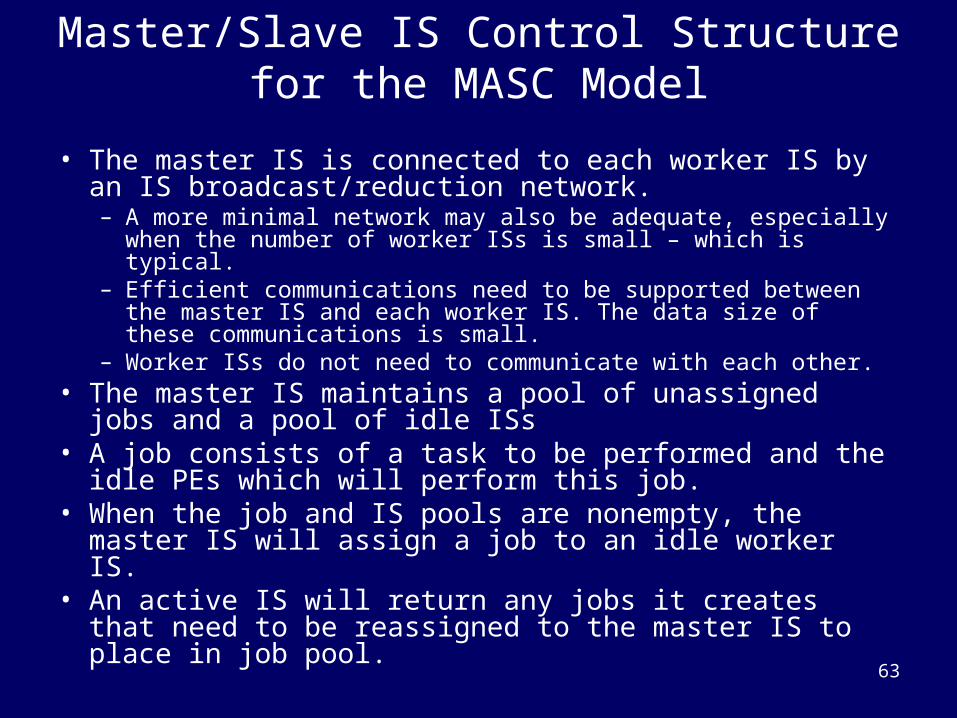
Master/Slave IS Control Structure for the MASC Model

• The master IS is connected to each worker IS by an IS broadcast/reduction network. – A more minimal network may also be adequate, especially when

the number of worker ISs is small – which is typical.– Efficient communications need to be supported between the

master IS and each worker IS. The data size of these communications is small.

– Worker ISs do not need to communicate with each other. • The master IS maintains a pool of unassigned jobs and a

pool of idle ISs• A job consists of a task to be performed and the idle PEs

which will perform this job.• When the job and IS pools are nonempty, the master IS

will assign a job to an idle worker IS.• An active IS will return any jobs it creates that need to be

reassigned to the master IS to place in job pool.

64

MASC Quickhull Algorithm

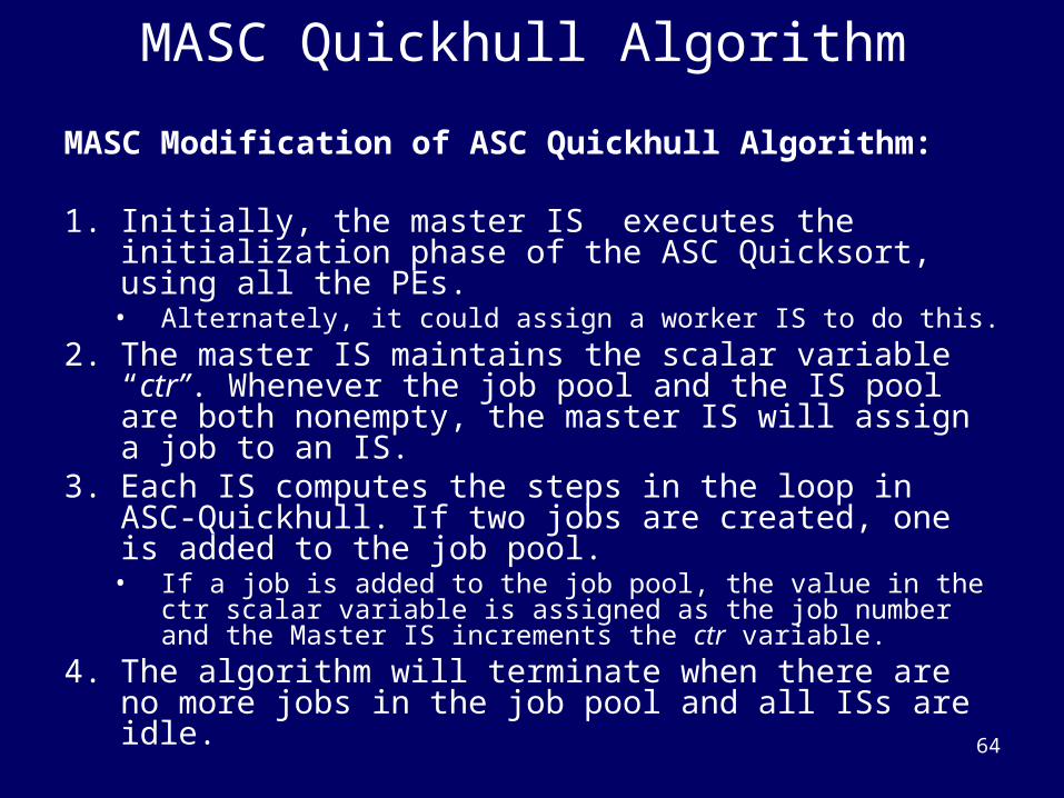
MASC Modification of ASC Quickhull Algorithm:

1. Initially, the master IS executes the initialization phase of the ASC Quicksort, using all the PEs.

• Alternately, it could assign a worker IS to do this.

2. The master IS maintains the scalar variable “ctr”. Whenever the job pool and the IS pool are both nonempty, the master IS will assign a job to an IS.

3. Each IS computes the steps in the loop in ASC-Quickhull. If two jobs are created, one is added to the job pool.

• If a job is added to the job pool, the value in the ctr scalar variable is assigned as the job number and the Master IS increments the ctr variable.

4. The algorithm will terminate when there are no more jobs in the job pool and all ISs are idle.

65

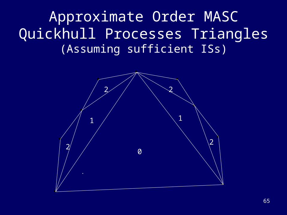
Approximate Order MASC Quickhull Processes Triangles(Assuming sufficient ISs)

0

1

2

2

1

2

2

66

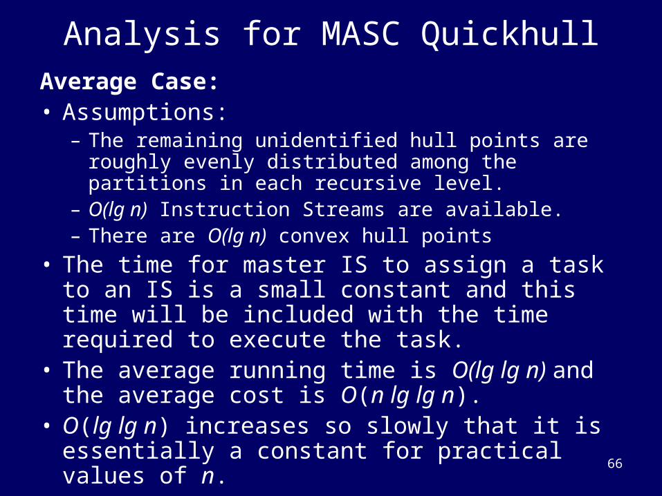
Analysis for MASC Quickhull

Average Case:• Assumptions:

– The remaining unidentified hull points are roughly evenly distributed among the partitions in each recursive level.

– O(lg n) Instruction Streams are available.– There are O(lg n) convex hull points

• The time for master IS to assign a task to an IS is a small constant and this time will be included with the time required to execute the task.

• The average running time is O(lg lg n) and the average cost is O(n lg lg n).

• O(lg lg n) increases so slowly that it is essentially a constant for practical values of n.

67

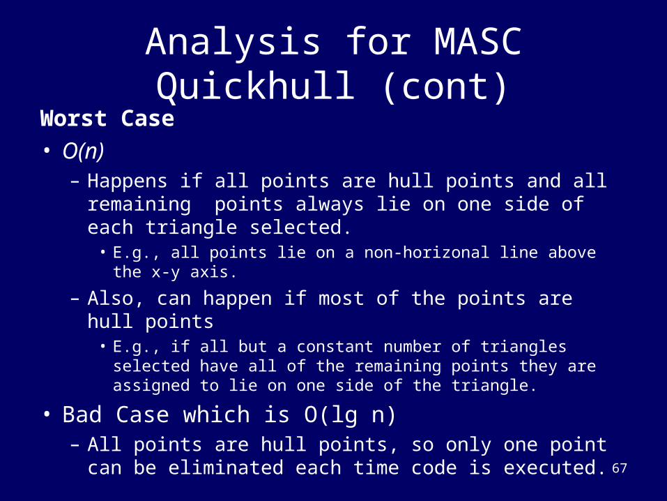
Analysis for MASC Quickhull (cont)

Worst Case• O(n)

– Happens if all points are hull points and all remaining points always lie on one side of each triangle selected.

• E.g., all points lie on a non-horizonal line above the x-y axis.

– Also, can happen if most of the points are hull points• E.g., if all but a constant number of triangles selected have

all of the remaining points they are assigned to lie on one side of the triangle.

• Bad Case which is O(lg n)– All points are hull points, so only one point can be

eliminated each time code is executed.

68

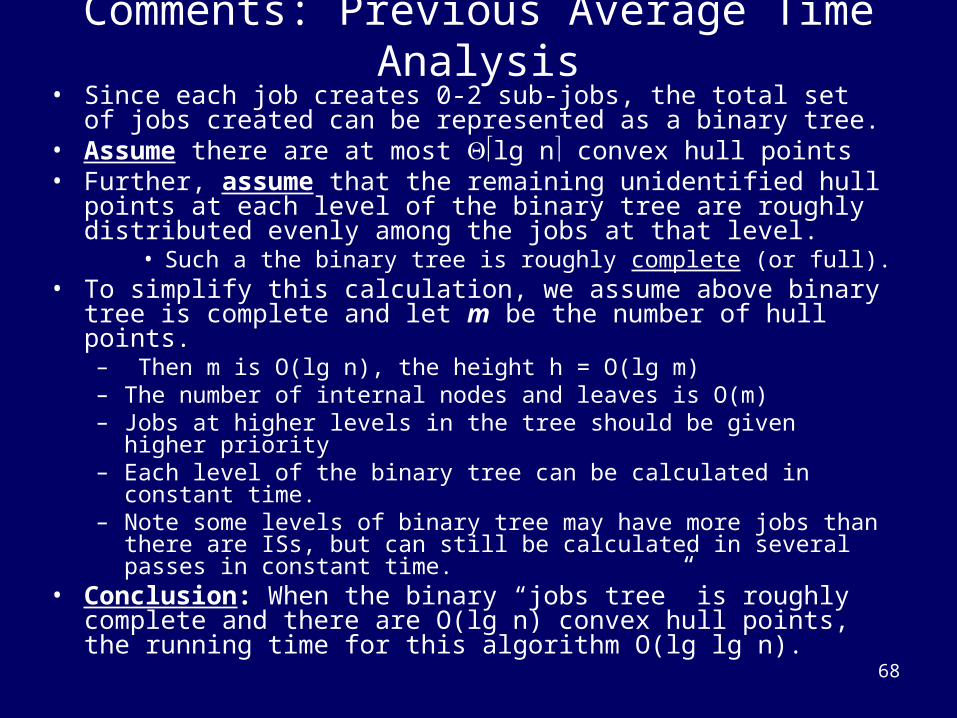
Comments: Previous Average Time Analysis• Since each job creates 0-2 sub-jobs, the total set of jobs created

can be represented as a binary tree.• Assume there are at most lg n convex hull points• Further, assume that the remaining unidentified hull points at each

level of the binary tree are roughly distributed evenly among the jobs at that level.

• Such a the binary tree is roughly complete (or full).• To simplify this calculation, we assume above binary tree is

complete and let m be the number of hull points.– Then m is O(lg n), the height h = O(lg m)– The number of internal nodes and leaves is O(m)– Jobs at higher levels in the tree should be given higher priority– Each level of the binary tree can be calculated in constant time.– Note some levels of binary tree may have more jobs than there are ISs,

but can still be calculated in several passes in constant time. • Conclusion: When the binary “jobs tree” is roughly complete and

there are O(lg n) convex hull points, the running time for this algorithm O(lg lg n).

69

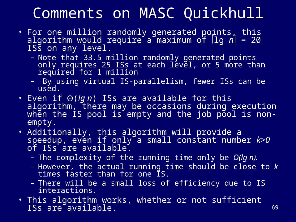
Comments on MASC Quickhull• For one million randomly generated points, this algorithm

would require a maximum of lg n = 20 ISs on any level. – Note that 33.5 million randomly generated points only

requires 25 ISs at each level, or 5 more than required for 1 million

– By using virtual IS-parallelism, fewer ISs can be used.• Even if (lg n) ISs are available for this algorithm, there

may be occasions during execution when the IS pool is empty and the job pool is non-empty.

• Additionally, this algorithm will provide a speedup, even if only a small constant number k>0 of ISs are available. – The complexity of the running time only be O(lg n).– However, the actual running time should be close to k

times faster than for one IS.– There will be a small loss of efficiency due to IS

interactions. • This algorithm works, whether or not sufficient ISs are

available.

70

Additional Comments on ASC and MASC Algorithms

• The full “convex hull” algorithm requires that an order (e.g., clockwise) list of convex hull points be returned.– Preceding algorithms for ASC and MASC can be

extended to handle this.

• This detail is omitted here to keep the algorithms simpler.– More information can be found in the paper “An

Associative Implementation of Classical Convex Hull Algorithms” by Atwah, Baker, and Akl and in Maher Atwah’s master’s thesis at KSU.

END OF SLIDE SET

72

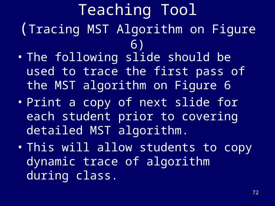
Teaching Tool(Tracing MST Algorithm on Figure 6)

• The following slide should be used to trace the first pass of the MST algorithm on Figure 6

• Print a copy of next slide for each student prior to covering detailed MST algorithm.

• This will allow students to copy dynamic trace of algorithm during class.

73

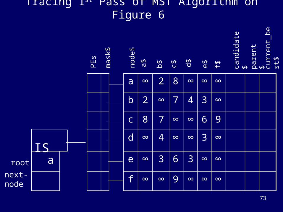
Tracing 1st Pass of MST Algorithm on Figure 6

curr

ent_

best

$

cand

idat

e$

next-node

a

IS

∞∞∞9∞∞f

∞∞363∞e

∞3∞∞4∞d

96∞∞78 c

∞347∞2b

∞∞∞82∞aP

Es

mas

k$

node

$

a$ b$ pare

nt$

rootc$ d$ e$ f$