similar matrices and diagonalization - ucfilespace...
TRANSCRIPT

Similar Matrices and Diagonalization
Linear AlgebraMATH 2076
Section 5.3 Similarity & Diagonalization 24 March 2017 1 / 10

Similar Matrices and Diagonalizable Matrices
Two n× n matrices A and B are similar if and only if there is an invertiblematrix P such that A = PBP−1 (and then we also haveB = P−1AP = QAQ−1 where Q = P−1).
An n × n matrix A is diagonalizable if and only if it is similar to a diagonalmatrix; that is, there are a diagonal matrix D and an invertible matrix Psuch that A = PDP−1.
An n × n matrix A is diagonalizable if and only if there is an eigenbasisassoc’d with A; that is, there is a basis {~v1, ~v2, . . . , ~vn} for Rn such thateach vector ~vi is an eigenvector for A. When this holds, say withA~vi = λi~vi , we have
A = PDP−1 where P =[~v1 ~v2 . . . ~vn
]and D =
λ1 0 . . . 00 λ2 . . . 0...
...... 0
0 0 . . . λn
.
Section 5.3 Similarity & Diagonalization 24 March 2017 2 / 10

Similar Matrices and Diagonalizable Matrices
Two n× n matrices A and B are similar if and only if there is an invertiblematrix P such that A = PBP−1
(and then we also haveB = P−1AP = QAQ−1 where Q = P−1).
An n × n matrix A is diagonalizable if and only if it is similar to a diagonalmatrix; that is, there are a diagonal matrix D and an invertible matrix Psuch that A = PDP−1.
An n × n matrix A is diagonalizable if and only if there is an eigenbasisassoc’d with A; that is, there is a basis {~v1, ~v2, . . . , ~vn} for Rn such thateach vector ~vi is an eigenvector for A. When this holds, say withA~vi = λi~vi , we have
A = PDP−1 where P =[~v1 ~v2 . . . ~vn
]and D =
λ1 0 . . . 00 λ2 . . . 0...
...... 0
0 0 . . . λn
.
Section 5.3 Similarity & Diagonalization 24 March 2017 2 / 10

Similar Matrices and Diagonalizable Matrices
Two n× n matrices A and B are similar if and only if there is an invertiblematrix P such that A = PBP−1 (and then we also haveB = P−1AP = QAQ−1 where Q = P−1).
An n × n matrix A is diagonalizable if and only if it is similar to a diagonalmatrix; that is, there are a diagonal matrix D and an invertible matrix Psuch that A = PDP−1.
An n × n matrix A is diagonalizable if and only if there is an eigenbasisassoc’d with A; that is, there is a basis {~v1, ~v2, . . . , ~vn} for Rn such thateach vector ~vi is an eigenvector for A. When this holds, say withA~vi = λi~vi , we have
A = PDP−1 where P =[~v1 ~v2 . . . ~vn
]and D =
λ1 0 . . . 00 λ2 . . . 0...
...... 0
0 0 . . . λn
.
Section 5.3 Similarity & Diagonalization 24 March 2017 2 / 10

Similar Matrices and Diagonalizable Matrices
Two n× n matrices A and B are similar if and only if there is an invertiblematrix P such that A = PBP−1 (and then we also haveB = P−1AP = QAQ−1 where Q = P−1).
An n × n matrix A is diagonalizable if and only if it is similar to a diagonalmatrix; that is,
there are a diagonal matrix D and an invertible matrix Psuch that A = PDP−1.
An n × n matrix A is diagonalizable if and only if there is an eigenbasisassoc’d with A; that is, there is a basis {~v1, ~v2, . . . , ~vn} for Rn such thateach vector ~vi is an eigenvector for A. When this holds, say withA~vi = λi~vi , we have
A = PDP−1 where P =[~v1 ~v2 . . . ~vn
]and D =
λ1 0 . . . 00 λ2 . . . 0...
...... 0
0 0 . . . λn
.
Section 5.3 Similarity & Diagonalization 24 March 2017 2 / 10

Similar Matrices and Diagonalizable Matrices
Two n× n matrices A and B are similar if and only if there is an invertiblematrix P such that A = PBP−1 (and then we also haveB = P−1AP = QAQ−1 where Q = P−1).
An n × n matrix A is diagonalizable if and only if it is similar to a diagonalmatrix; that is, there are a diagonal matrix D and an invertible matrix Psuch that A = PDP−1.
An n × n matrix A is diagonalizable if and only if there is an eigenbasisassoc’d with A; that is, there is a basis {~v1, ~v2, . . . , ~vn} for Rn such thateach vector ~vi is an eigenvector for A. When this holds, say withA~vi = λi~vi , we have
A = PDP−1 where P =[~v1 ~v2 . . . ~vn
]and D =
λ1 0 . . . 00 λ2 . . . 0...
...... 0
0 0 . . . λn
.
Section 5.3 Similarity & Diagonalization 24 March 2017 2 / 10

Similar Matrices and Diagonalizable Matrices
Two n× n matrices A and B are similar if and only if there is an invertiblematrix P such that A = PBP−1 (and then we also haveB = P−1AP = QAQ−1 where Q = P−1).
An n × n matrix A is diagonalizable if and only if it is similar to a diagonalmatrix; that is, there are a diagonal matrix D and an invertible matrix Psuch that A = PDP−1.
An n × n matrix A is diagonalizable if and only if there is an eigenbasisassoc’d with A; that is,
there is a basis {~v1, ~v2, . . . , ~vn} for Rn such thateach vector ~vi is an eigenvector for A. When this holds, say withA~vi = λi~vi , we have
A = PDP−1 where P =[~v1 ~v2 . . . ~vn
]and D =
λ1 0 . . . 00 λ2 . . . 0...
...... 0
0 0 . . . λn
.
Section 5.3 Similarity & Diagonalization 24 March 2017 2 / 10

Similar Matrices and Diagonalizable Matrices
Two n× n matrices A and B are similar if and only if there is an invertiblematrix P such that A = PBP−1 (and then we also haveB = P−1AP = QAQ−1 where Q = P−1).
An n × n matrix A is diagonalizable if and only if it is similar to a diagonalmatrix; that is, there are a diagonal matrix D and an invertible matrix Psuch that A = PDP−1.
An n × n matrix A is diagonalizable if and only if there is an eigenbasisassoc’d with A; that is, there is a basis {~v1, ~v2, . . . , ~vn} for Rn such thateach vector ~vi is an eigenvector for A.
When this holds, say withA~vi = λi~vi , we have
A = PDP−1 where P =[~v1 ~v2 . . . ~vn
]and D =
λ1 0 . . . 00 λ2 . . . 0...
...... 0
0 0 . . . λn
.
Section 5.3 Similarity & Diagonalization 24 March 2017 2 / 10

Similar Matrices and Diagonalizable Matrices
Two n× n matrices A and B are similar if and only if there is an invertiblematrix P such that A = PBP−1 (and then we also haveB = P−1AP = QAQ−1 where Q = P−1).
An n × n matrix A is diagonalizable if and only if it is similar to a diagonalmatrix; that is, there are a diagonal matrix D and an invertible matrix Psuch that A = PDP−1.
An n × n matrix A is diagonalizable if and only if there is an eigenbasisassoc’d with A; that is, there is a basis {~v1, ~v2, . . . , ~vn} for Rn such thateach vector ~vi is an eigenvector for A. When this holds, say withA~vi = λi~vi , we have
A = PDP−1 where P =[~v1 ~v2 . . . ~vn
]and D =
λ1 0 . . . 00 λ2 . . . 0...
...... 0
0 0 . . . λn
.
Section 5.3 Similarity & Diagonalization 24 March 2017 2 / 10

Similar Matrices and Diagonalizable Matrices
Two n× n matrices A and B are similar if and only if there is an invertiblematrix P such that A = PBP−1 (and then we also haveB = P−1AP = QAQ−1 where Q = P−1).
An n × n matrix A is diagonalizable if and only if it is similar to a diagonalmatrix; that is, there are a diagonal matrix D and an invertible matrix Psuch that A = PDP−1.
An n × n matrix A is diagonalizable if and only if there is an eigenbasisassoc’d with A; that is, there is a basis {~v1, ~v2, . . . , ~vn} for Rn such thateach vector ~vi is an eigenvector for A. When this holds, say withA~vi = λi~vi , we have
A = PDP−1 where P =[~v1 ~v2 . . . ~vn
]and D =
λ1 0 . . . 00 λ2 . . . 0...
...... 0
0 0 . . . λn
.Section 5.3 Similarity & Diagonalization 24 March 2017 2 / 10

A 2× 2 Example
The matrix A =
[1 24 3
]has simple eigenvalues λ1 = 5 and λ2 = −1 with
assoc’d eigenvectors ~v1 =
[12
]and ~v2 =
[1−1
].
Therefore,
A = PDP−1 where P =
[1 12 −1
]and D =
[5 00 −1
].
But what does this mean??
Section 5.3 Similarity & Diagonalization 24 March 2017 3 / 10

A 2× 2 Example
The matrix A =
[1 24 3
]has simple eigenvalues λ1 = 5 and λ2 = −1 with
assoc’d eigenvectors ~v1 =
[12
]and ~v2 =
[1−1
].
Therefore,
A = PDP−1 where P =
[1 12 −1
]and D =
[5 00 −1
].
But what does this mean??
Section 5.3 Similarity & Diagonalization 24 March 2017 3 / 10

A 2× 2 Example
The matrix A =
[1 24 3
]has simple eigenvalues λ1 = 5 and λ2 = −1 with
assoc’d eigenvectors ~v1 =
[12
]and ~v2 =
[1−1
].
Therefore,
A = PDP−1 where P =
[1 12 −1
]and D =
[5 00 −1
].
But what does this mean??
Section 5.3 Similarity & Diagonalization 24 March 2017 3 / 10

A 3× 3 Example
The matrix A =
4 −1 0−1 5 −10 −1 4
has simple eigenvalues 3, 4, 6 with
associated eigenvectors
~v1 =
111
, ~v2 =−10
1
, ~v3 = 1−21
.Therefore,
A = PDP−1 where P =
1 −1 11 0 −21 1 1
and D =
3 0 00 4 00 0 6
.
But what does this mean??
Section 5.3 Similarity & Diagonalization 24 March 2017 4 / 10

A 3× 3 Example
The matrix A =
4 −1 0−1 5 −10 −1 4
has simple eigenvalues 3, 4, 6 with
associated eigenvectors ~v1 =
111
, ~v2 =−10
1
, ~v3 = 1−21
.
Therefore,
A = PDP−1 where P =
1 −1 11 0 −21 1 1
and D =
3 0 00 4 00 0 6
.
But what does this mean??
Section 5.3 Similarity & Diagonalization 24 March 2017 4 / 10

A 3× 3 Example
The matrix A =
4 −1 0−1 5 −10 −1 4
has simple eigenvalues 3, 4, 6 with
associated eigenvectors ~v1 =
111
, ~v2 =−10
1
, ~v3 = 1−21
.Therefore,
A = PDP−1 where P =
1 −1 11 0 −21 1 1
and D =
3 0 00 4 00 0 6
.
But what does this mean??
Section 5.3 Similarity & Diagonalization 24 March 2017 4 / 10

A 3× 3 Example
The matrix A =
4 −1 0−1 5 −10 −1 4
has simple eigenvalues 3, 4, 6 with
associated eigenvectors ~v1 =
111
, ~v2 =−10
1
, ~v3 = 1−21
.Therefore,
A = PDP−1 where P =
1 −1 11 0 −21 1 1
and D =
3 0 00 4 00 0 6
.
But what does this mean??
Section 5.3 Similarity & Diagonalization 24 March 2017 4 / 10

3× 3 Matrices with Simple and Double Eigenvalues
A2 =
1 4 40 3 20 2 3
has one simple eigenvalue 5 and one double eigenvalue 2
with associated eigenvectors ~v1 =
211
, ~v2 =100
, ~v3 = 0
1−1
.{~v1, ~v2, ~v3} is an eigenbasis assoc’d with A2, so A2 is diagonalizable.
A3 =
5 −6 01 −2 04 6 −1
has one simple eigenvalue 4 and one double
eigenvalue −1 with associated eigenvectors ~v1 =
616
, ~v2 =001
.There is no eigenbasis assoc’d with A3, so A3 is not diagonalizable.
Section 5.3 Similarity & Diagonalization 24 March 2017 5 / 10

3× 3 Matrices with Simple and Double Eigenvalues
A2 =
1 4 40 3 20 2 3
has one simple eigenvalue 5 and one double eigenvalue 2
with associated eigenvectors
~v1 =
211
, ~v2 =100
, ~v3 = 0
1−1
.{~v1, ~v2, ~v3} is an eigenbasis assoc’d with A2, so A2 is diagonalizable.
A3 =
5 −6 01 −2 04 6 −1
has one simple eigenvalue 4 and one double
eigenvalue −1 with associated eigenvectors ~v1 =
616
, ~v2 =001
.There is no eigenbasis assoc’d with A3, so A3 is not diagonalizable.
Section 5.3 Similarity & Diagonalization 24 March 2017 5 / 10

3× 3 Matrices with Simple and Double Eigenvalues
A2 =
1 4 40 3 20 2 3
has one simple eigenvalue 5 and one double eigenvalue 2
with associated eigenvectors ~v1 =
211
, ~v2 =100
, ~v3 = 0
1−1
.
{~v1, ~v2, ~v3} is an eigenbasis assoc’d with A2, so A2 is diagonalizable.
A3 =
5 −6 01 −2 04 6 −1
has one simple eigenvalue 4 and one double
eigenvalue −1 with associated eigenvectors ~v1 =
616
, ~v2 =001
.There is no eigenbasis assoc’d with A3, so A3 is not diagonalizable.
Section 5.3 Similarity & Diagonalization 24 March 2017 5 / 10

3× 3 Matrices with Simple and Double Eigenvalues
A2 =
1 4 40 3 20 2 3
has one simple eigenvalue 5 and one double eigenvalue 2
with associated eigenvectors ~v1 =
211
, ~v2 =100
, ~v3 = 0
1−1
.{~v1, ~v2, ~v3} is an eigenbasis assoc’d with A2, so
A2 is diagonalizable.
A3 =
5 −6 01 −2 04 6 −1
has one simple eigenvalue 4 and one double
eigenvalue −1 with associated eigenvectors ~v1 =
616
, ~v2 =001
.There is no eigenbasis assoc’d with A3, so A3 is not diagonalizable.
Section 5.3 Similarity & Diagonalization 24 March 2017 5 / 10

3× 3 Matrices with Simple and Double Eigenvalues
A2 =
1 4 40 3 20 2 3
has one simple eigenvalue 5 and one double eigenvalue 2
with associated eigenvectors ~v1 =
211
, ~v2 =100
, ~v3 = 0
1−1
.{~v1, ~v2, ~v3} is an eigenbasis assoc’d with A2, so A2 is diagonalizable.
A3 =
5 −6 01 −2 04 6 −1
has one simple eigenvalue 4 and one double
eigenvalue −1 with associated eigenvectors ~v1 =
616
, ~v2 =001
.There is no eigenbasis assoc’d with A3, so A3 is not diagonalizable.
Section 5.3 Similarity & Diagonalization 24 March 2017 5 / 10

3× 3 Matrices with Simple and Double Eigenvalues
A2 =
1 4 40 3 20 2 3
has one simple eigenvalue 5 and one double eigenvalue 2
with associated eigenvectors ~v1 =
211
, ~v2 =100
, ~v3 = 0
1−1
.{~v1, ~v2, ~v3} is an eigenbasis assoc’d with A2, so A2 is diagonalizable.
A3 =
5 −6 01 −2 04 6 −1
has one simple eigenvalue 4 and one double
eigenvalue −1 with associated eigenvectors
~v1 =
616
, ~v2 =001
.There is no eigenbasis assoc’d with A3, so A3 is not diagonalizable.
Section 5.3 Similarity & Diagonalization 24 March 2017 5 / 10

3× 3 Matrices with Simple and Double Eigenvalues
A2 =
1 4 40 3 20 2 3
has one simple eigenvalue 5 and one double eigenvalue 2
with associated eigenvectors ~v1 =
211
, ~v2 =100
, ~v3 = 0
1−1
.{~v1, ~v2, ~v3} is an eigenbasis assoc’d with A2, so A2 is diagonalizable.
A3 =
5 −6 01 −2 04 6 −1
has one simple eigenvalue 4 and one double
eigenvalue −1 with associated eigenvectors ~v1 =
616
, ~v2 =001
.
There is no eigenbasis assoc’d with A3, so A3 is not diagonalizable.
Section 5.3 Similarity & Diagonalization 24 March 2017 5 / 10

3× 3 Matrices with Simple and Double Eigenvalues
A2 =
1 4 40 3 20 2 3
has one simple eigenvalue 5 and one double eigenvalue 2
with associated eigenvectors ~v1 =
211
, ~v2 =100
, ~v3 = 0
1−1
.{~v1, ~v2, ~v3} is an eigenbasis assoc’d with A2, so A2 is diagonalizable.
A3 =
5 −6 01 −2 04 6 −1
has one simple eigenvalue 4 and one double
eigenvalue −1 with associated eigenvectors ~v1 =
616
, ~v2 =001
.There is no eigenbasis assoc’d with A3, so
A3 is not diagonalizable.
Section 5.3 Similarity & Diagonalization 24 March 2017 5 / 10

3× 3 Matrices with Simple and Double Eigenvalues
A2 =
1 4 40 3 20 2 3
has one simple eigenvalue 5 and one double eigenvalue 2
with associated eigenvectors ~v1 =
211
, ~v2 =100
, ~v3 = 0
1−1
.{~v1, ~v2, ~v3} is an eigenbasis assoc’d with A2, so A2 is diagonalizable.
A3 =
5 −6 01 −2 04 6 −1
has one simple eigenvalue 4 and one double
eigenvalue −1 with associated eigenvectors ~v1 =
616
, ~v2 =001
.There is no eigenbasis assoc’d with A3, so A3 is not diagonalizable.
Section 5.3 Similarity & Diagonalization 24 March 2017 5 / 10

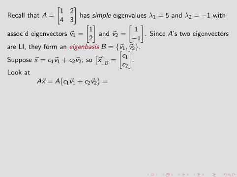
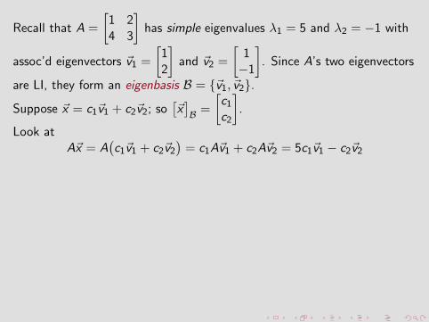
Recall that A =
[1 24 3
]has simple eigenvalues λ1 = 5 and λ2 = −1 with
assoc’d eigenvectors
~v1 =
[12
]and ~v2 =
[1−1
]. Since A’s two eigenvectors
are LI, they form an eigenbasis B = {~v1, ~v2}.
Suppose ~x = c1~v1 + c2~v2; so[~x]B =
[c1c2
].
Look atA~x =
A(c1~v1 + c2~v2
)=
c1A~v1 + c2A~v2 =
5c1~v1 − c2~v2
which says that
[A~x]B=
[5c1−c2
]=
[5 00 −1
] [c1c2
]=
[5 00 −1
] [~x]B.
Thus using B-coordinates, the action of A is just multiplication by thediagonal matrix
D =
[5 00 −1
]=
[λ1 00 λ2
].
But, how do we get A~x?

Recall that A =
[1 24 3
]has simple eigenvalues λ1 = 5 and λ2 = −1 with
assoc’d eigenvectors ~v1 =
[12
]and ~v2 =
[1−1
].
Since A’s two eigenvectors
are LI, they form an eigenbasis B = {~v1, ~v2}.
Suppose ~x = c1~v1 + c2~v2; so[~x]B =
[c1c2
].
Look atA~x =
A(c1~v1 + c2~v2
)=
c1A~v1 + c2A~v2 =
5c1~v1 − c2~v2
which says that
[A~x]B=
[5c1−c2
]=
[5 00 −1
] [c1c2
]=
[5 00 −1
] [~x]B.
Thus using B-coordinates, the action of A is just multiplication by thediagonal matrix
D =
[5 00 −1
]=
[λ1 00 λ2
].
But, how do we get A~x?

Recall that A =
[1 24 3
]has simple eigenvalues λ1 = 5 and λ2 = −1 with
assoc’d eigenvectors ~v1 =
[12
]and ~v2 =
[1−1
]. Since A’s two eigenvectors
are LI, they form an eigenbasis B = {~v1, ~v2}.
Suppose ~x = c1~v1 + c2~v2; so[~x]B =
[c1c2
].
Look atA~x =
A(c1~v1 + c2~v2
)=
c1A~v1 + c2A~v2 =
5c1~v1 − c2~v2
which says that
[A~x]B=
[5c1−c2
]=
[5 00 −1
] [c1c2
]=
[5 00 −1
] [~x]B.
Thus using B-coordinates, the action of A is just multiplication by thediagonal matrix
D =
[5 00 −1
]=
[λ1 00 λ2
].
But, how do we get A~x?

Recall that A =
[1 24 3
]has simple eigenvalues λ1 = 5 and λ2 = −1 with
assoc’d eigenvectors ~v1 =
[12
]and ~v2 =
[1−1
]. Since A’s two eigenvectors
are LI, they form an eigenbasis B = {~v1, ~v2}.
Suppose ~x = c1~v1 + c2~v2; so
[~x]B =
[c1c2
].
Look atA~x =
A(c1~v1 + c2~v2
)=
c1A~v1 + c2A~v2 =
5c1~v1 − c2~v2
which says that
[A~x]B=
[5c1−c2
]=
[5 00 −1
] [c1c2
]=
[5 00 −1
] [~x]B.
Thus using B-coordinates, the action of A is just multiplication by thediagonal matrix
D =
[5 00 −1
]=
[λ1 00 λ2
].
But, how do we get A~x?

Recall that A =
[1 24 3
]has simple eigenvalues λ1 = 5 and λ2 = −1 with
assoc’d eigenvectors ~v1 =
[12
]and ~v2 =
[1−1
]. Since A’s two eigenvectors
are LI, they form an eigenbasis B = {~v1, ~v2}.
Suppose ~x = c1~v1 + c2~v2; so[~x]B =
[c1c2
].
Look atA~x =
A(c1~v1 + c2~v2
)=
c1A~v1 + c2A~v2 =
5c1~v1 − c2~v2
which says that
[A~x]B=
[5c1−c2
]=
[5 00 −1
] [c1c2
]=
[5 00 −1
] [~x]B.
Thus using B-coordinates, the action of A is just multiplication by thediagonal matrix
D =
[5 00 −1
]=
[λ1 00 λ2
].
But, how do we get A~x?

Recall that A =
[1 24 3
]has simple eigenvalues λ1 = 5 and λ2 = −1 with
assoc’d eigenvectors ~v1 =
[12
]and ~v2 =
[1−1
]. Since A’s two eigenvectors
are LI, they form an eigenbasis B = {~v1, ~v2}.
Suppose ~x = c1~v1 + c2~v2; so[~x]B =
[c1c2
].
Look atA~x =
A(c1~v1 + c2~v2
)=
c1A~v1 + c2A~v2 =
5c1~v1 − c2~v2
which says that
[A~x]B=
[5c1−c2
]=
[5 00 −1
] [c1c2
]=
[5 00 −1
] [~x]B.
Thus using B-coordinates, the action of A is just multiplication by thediagonal matrix
D =
[5 00 −1
]=
[λ1 00 λ2
].
But, how do we get A~x?
Recall that A =
[1 24 3
]has simple eigenvalues λ1 = 5 and λ2 = −1 with
assoc’d eigenvectors ~v1 =
[12
]and ~v2 =
[1−1
]. Since A’s two eigenvectors
are LI, they form an eigenbasis B = {~v1, ~v2}.
Suppose ~x = c1~v1 + c2~v2; so[~x]B =
[c1c2
].
Look atA~x = A
(c1~v1 + c2~v2
)=
c1A~v1 + c2A~v2 =
5c1~v1 − c2~v2
which says that
[A~x]B=
[5c1−c2
]=
[5 00 −1
] [c1c2
]=
[5 00 −1
] [~x]B.
Thus using B-coordinates, the action of A is just multiplication by thediagonal matrix
D =
[5 00 −1
]=
[λ1 00 λ2
].
But, how do we get A~x?

Recall that A =
[1 24 3
]has simple eigenvalues λ1 = 5 and λ2 = −1 with
assoc’d eigenvectors ~v1 =
[12
]and ~v2 =
[1−1
]. Since A’s two eigenvectors
are LI, they form an eigenbasis B = {~v1, ~v2}.
Suppose ~x = c1~v1 + c2~v2; so[~x]B =
[c1c2
].
Look atA~x = A
(c1~v1 + c2~v2
)= c1A~v1 + c2A~v2 =
5c1~v1 − c2~v2
which says that
[A~x]B=
[5c1−c2
]=
[5 00 −1
] [c1c2
]=
[5 00 −1
] [~x]B.
Thus using B-coordinates, the action of A is just multiplication by thediagonal matrix
D =
[5 00 −1
]=
[λ1 00 λ2
].
But, how do we get A~x?
Recall that A =
[1 24 3
]has simple eigenvalues λ1 = 5 and λ2 = −1 with
assoc’d eigenvectors ~v1 =
[12
]and ~v2 =
[1−1
]. Since A’s two eigenvectors
are LI, they form an eigenbasis B = {~v1, ~v2}.
Suppose ~x = c1~v1 + c2~v2; so[~x]B =
[c1c2
].
Look atA~x = A
(c1~v1 + c2~v2
)= c1A~v1 + c2A~v2 = 5c1~v1 − c2~v2
which says that
[A~x]B=
[5c1−c2
]=
[5 00 −1
] [c1c2
]=
[5 00 −1
] [~x]B.
Thus using B-coordinates, the action of A is just multiplication by thediagonal matrix
D =
[5 00 −1
]=
[λ1 00 λ2
].
But, how do we get A~x?

Recall that A =
[1 24 3
]has simple eigenvalues λ1 = 5 and λ2 = −1 with
assoc’d eigenvectors ~v1 =
[12
]and ~v2 =
[1−1
]. Since A’s two eigenvectors
are LI, they form an eigenbasis B = {~v1, ~v2}.
Suppose ~x = c1~v1 + c2~v2; so[~x]B =
[c1c2
].
Look atA~x = A
(c1~v1 + c2~v2
)= c1A~v1 + c2A~v2 = 5c1~v1 − c2~v2
which says that[A~x]B=
[5c1−c2
]=
[5 00 −1
] [c1c2
]=
[5 00 −1
] [~x]B.
Thus using B-coordinates, the action of A is just multiplication by thediagonal matrix
D =
[5 00 −1
]=
[λ1 00 λ2
].
But, how do we get A~x?

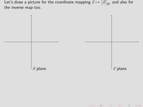
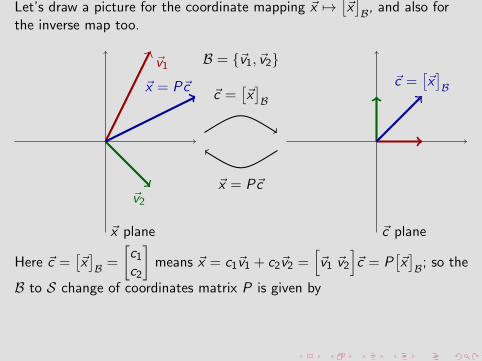
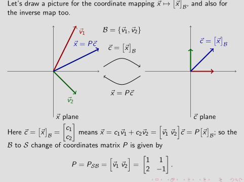
Let’s draw a picture for the coordinate mapping ~x 7→[~x]B, and also for
the inverse map too.
~x plane ~c plane
~c =[~x]B
~x = P~c
~v1
~v2
B = {~v1, ~v2}
~x = P~c ~c =[~x]B
Here ~c =[~x]B =
[c1c2
]means ~x = c1~v1 + c2~v2 =
[~v1 ~v2
]~c = P
[~x]B; so the
B to S change of coordinates matrix P is given by
P = PSB =
[~v1 ~v2
]=
[1 12 −1
].

Let’s draw a picture for the coordinate mapping ~x 7→[~x]B, and also for
the inverse map too.
~x plane ~c plane
~c =[~x]B
~x = P~c
~v1
~v2
B = {~v1, ~v2}
~x = P~c ~c =[~x]B
Here ~c =[~x]B =
[c1c2
]means
~x = c1~v1 + c2~v2 =[~v1 ~v2
]~c = P
[~x]B; so the
B to S change of coordinates matrix P is given by
P = PSB =
[~v1 ~v2
]=
[1 12 −1
].

Let’s draw a picture for the coordinate mapping ~x 7→[~x]B, and also for
the inverse map too.
~x plane ~c plane
~c =[~x]B
~x = P~c
~v1
~v2
B = {~v1, ~v2}
~x = P~c ~c =[~x]B
Here ~c =[~x]B =
[c1c2
]means ~x = c1~v1 + c2~v2 =
[~v1 ~v2
]~c = P
[~x]B; so
the
B to S change of coordinates matrix P is given by
P = PSB =
[~v1 ~v2
]=
[1 12 −1
].
Let’s draw a picture for the coordinate mapping ~x 7→[~x]B, and also for
the inverse map too.
~x plane ~c plane
~c =[~x]B
~x = P~c
~v1
~v2
B = {~v1, ~v2}
~x = P~c ~c =[~x]B
Here ~c =[~x]B =
[c1c2
]means ~x = c1~v1 + c2~v2 =
[~v1 ~v2
]~c = P
[~x]B; so the
B to S change of coordinates matrix P is given by
P = PSB =
[~v1 ~v2
]=
[1 12 −1
].

Let’s draw a picture for the coordinate mapping ~x 7→[~x]B, and also for
the inverse map too.
~x plane ~c plane
~c =[~x]B
~x = P~c
~v1
~v2
B = {~v1, ~v2}
~x = P~c ~c =[~x]B
Here ~c =[~x]B =
[c1c2
]means ~x = c1~v1 + c2~v2 =
[~v1 ~v2
]~c = P
[~x]B; so the
B to S change of coordinates matrix P is given by
P = PSB =[~v1 ~v2
]=
[1 12 −1
].

From an earlier slide: WTF A~x and we know[A~x]B= D
[~x]B where D =
[5 00 −1
]and A =
[1 24 3
]and we have an eigenbasis assoc’d with A given by
B = {~v1, ~v2} where ~v1 =
[12
], ~v2 =
[1−1
].
Recall that for any vector ~w in R2 we have~w = P
[~w]B and
[~w]B = P−1~w
where the B to S change of coordinates matrix P is given by
P = PSB =
[~v1 ~v2
]=
[1 12 −1
].
Thus [~x]B = P−1~x and
A~x =
P[A~x]B=
PD[~x]B =
PDP−1~x .
So,
A = PDP−1 where D =
[5 00 −1
]=
[λ1 00 λ2
], P =
[~v1 ~v2
]=
[1 12 −1
].
Thus A and D are similar matrices. How to “see” the LT ~x 7→ A~x?

From an earlier slide: WTF A~x and we know[A~x]B= D
[~x]B where D =
[5 00 −1
]and A =
[1 24 3
]and we have an eigenbasis assoc’d with A given by
B = {~v1, ~v2} where ~v1 =
[12
], ~v2 =
[1−1
].
Recall that for any vector ~w in R2 we have
~w = P[~w]B and
[~w]B = P−1~w
where the B to S change of coordinates matrix P is given by
P = PSB =
[~v1 ~v2
]=
[1 12 −1
].
Thus [~x]B = P−1~x and
A~x =
P[A~x]B=
PD[~x]B =
PDP−1~x .
So,
A = PDP−1 where D =
[5 00 −1
]=
[λ1 00 λ2
], P =
[~v1 ~v2
]=
[1 12 −1
].
Thus A and D are similar matrices. How to “see” the LT ~x 7→ A~x?

From an earlier slide: WTF A~x and we know[A~x]B= D
[~x]B where D =
[5 00 −1
]and A =
[1 24 3
]and we have an eigenbasis assoc’d with A given by
B = {~v1, ~v2} where ~v1 =
[12
], ~v2 =
[1−1
].
Recall that for any vector ~w in R2 we have~w = P
[~w]B and
[~w]B = P−1~w
where the B to S change of coordinates matrix P is given by
P = PSB =
[~v1 ~v2
]=
[1 12 −1
].
Thus [~x]B = P−1~x and
A~x =
P[A~x]B=
PD[~x]B =
PDP−1~x .
So,
A = PDP−1 where D =
[5 00 −1
]=
[λ1 00 λ2
], P =
[~v1 ~v2
]=
[1 12 −1
].
Thus A and D are similar matrices. How to “see” the LT ~x 7→ A~x?

From an earlier slide: WTF A~x and we know[A~x]B= D
[~x]B where D =
[5 00 −1
]and A =
[1 24 3
]and we have an eigenbasis assoc’d with A given by
B = {~v1, ~v2} where ~v1 =
[12
], ~v2 =
[1−1
].
Recall that for any vector ~w in R2 we have~w = P
[~w]B and
[~w]B = P−1~w
where the B to S change of coordinates matrix P is given by
P = PSB =[~v1 ~v2
]=
[1 12 −1
].
Thus [~x]B = P−1~x and A~x =
P[A~x]B=
PD[~x]B =
PDP−1~x .
So,
A = PDP−1 where D =
[5 00 −1
]=
[λ1 00 λ2
], P =
[~v1 ~v2
]=
[1 12 −1
].
Thus A and D are similar matrices. How to “see” the LT ~x 7→ A~x?

From an earlier slide: WTF A~x and we know[A~x]B= D
[~x]B where D =
[5 00 −1
]and A =
[1 24 3
]and we have an eigenbasis assoc’d with A given by
B = {~v1, ~v2} where ~v1 =
[12
], ~v2 =
[1−1
].
Recall that for any vector ~w in R2 we have~w = P
[~w]B and
[~w]B = P−1~w
where the B to S change of coordinates matrix P is given by
P = PSB =[~v1 ~v2
]=
[1 12 −1
].
Thus [~x]B = P−1~x and A~x = P
[A~x]B=
PD[~x]B =
PDP−1~x .
So,
A = PDP−1 where D =
[5 00 −1
]=
[λ1 00 λ2
], P =
[~v1 ~v2
]=
[1 12 −1
].
Thus A and D are similar matrices. How to “see” the LT ~x 7→ A~x?

From an earlier slide: WTF A~x and we know[A~x]B= D
[~x]B where D =
[5 00 −1
]and A =
[1 24 3
]and we have an eigenbasis assoc’d with A given by
B = {~v1, ~v2} where ~v1 =
[12
], ~v2 =
[1−1
].
Recall that for any vector ~w in R2 we have~w = P
[~w]B and
[~w]B = P−1~w
where the B to S change of coordinates matrix P is given by
P = PSB =[~v1 ~v2
]=
[1 12 −1
].
Thus [~x]B = P−1~x and A~x = P
[A~x]B= PD
[~x]B =
PDP−1~x .
So,
A = PDP−1 where D =
[5 00 −1
]=
[λ1 00 λ2
], P =
[~v1 ~v2
]=
[1 12 −1
].
Thus A and D are similar matrices. How to “see” the LT ~x 7→ A~x?

From an earlier slide: WTF A~x and we know[A~x]B= D
[~x]B where D =
[5 00 −1
]and A =
[1 24 3
]and we have an eigenbasis assoc’d with A given by
B = {~v1, ~v2} where ~v1 =
[12
], ~v2 =
[1−1
].
Recall that for any vector ~w in R2 we have~w = P
[~w]B and
[~w]B = P−1~w
where the B to S change of coordinates matrix P is given by
P = PSB =[~v1 ~v2
]=
[1 12 −1
].
Thus [~x]B = P−1~x and A~x = P
[A~x]B= PD
[~x]B = PDP−1~x .
So,
A = PDP−1 where D =
[5 00 −1
]=
[λ1 00 λ2
], P =
[~v1 ~v2
]=
[1 12 −1
].
Thus A and D are similar matrices.
How to “see” the LT ~x 7→ A~x?

From an earlier slide: WTF A~x and we know[A~x]B= D
[~x]B where D =
[5 00 −1
]and A =
[1 24 3
]and we have an eigenbasis assoc’d with A given by
B = {~v1, ~v2} where ~v1 =
[12
], ~v2 =
[1−1
].
Recall that for any vector ~w in R2 we have~w = P
[~w]B and
[~w]B = P−1~w
where the B to S change of coordinates matrix P is given by
P = PSB =[~v1 ~v2
]=
[1 12 −1
].
Thus [~x]B = P−1~x and A~x = P
[A~x]B= PD
[~x]B = PDP−1~x .
So,
A = PDP−1 where D =
[5 00 −1
]=
[λ1 00 λ2
], P =
[~v1 ~v2
]=
[1 12 −1
].
Thus A and D are similar matrices. How to “see” the LT ~x 7→ A~x?

~c plane
~x plane
~d plane
~y plane
~y = A~x
A =
[1 24 3
]
~d = D~c
D =
[5 00 −1
]
~c =[~x]B ~x = P~c ~d =
[~y]B~y = P ~d
~v1
~v2

Diagonalizable Matrices
An n × n matrix A is diagonalizable if and only if there is an eigenbasisassoc’d with A. This holds if, say, A has n distinct (real) eigenvalues,because then the assoc’d eigenvalues are LI and hence form a basis.
In general, there is an eigenbasis assoc’d with A if and only if thedimensions of the eigenspaces for A add up to n.
Suppose λ is an eigenvalue for A. This means that λ is a zero for thecharacteristic polynomial pA of A. Therefore, we can factor pA as
p(t) = (t − λ)mq(t) for some m.
We call m the algebraic multiplicity of the eigenvalue λ.
We always have 1 ≤ dim E(λ) ≤ m.
We call dim E(λ) the geometric multiplicity of the eigenvalue λ.
There is an eigenbasis assoc’d with A if and only if for every eigenvalue λthe geometric multiplicity of λ equals the algebraic multiplicity of λ.
Section 5.3 Similarity & Diagonalization 24 March 2017 10 / 10

Diagonalizable Matrices
An n × n matrix A is diagonalizable if and only if there is an eigenbasisassoc’d with A.
This holds if, say, A has n distinct (real) eigenvalues,because then the assoc’d eigenvalues are LI and hence form a basis.
In general, there is an eigenbasis assoc’d with A if and only if thedimensions of the eigenspaces for A add up to n.
Suppose λ is an eigenvalue for A. This means that λ is a zero for thecharacteristic polynomial pA of A. Therefore, we can factor pA as
p(t) = (t − λ)mq(t) for some m.
We call m the algebraic multiplicity of the eigenvalue λ.
We always have 1 ≤ dim E(λ) ≤ m.
We call dim E(λ) the geometric multiplicity of the eigenvalue λ.
There is an eigenbasis assoc’d with A if and only if for every eigenvalue λthe geometric multiplicity of λ equals the algebraic multiplicity of λ.
Section 5.3 Similarity & Diagonalization 24 March 2017 10 / 10

Diagonalizable Matrices
An n × n matrix A is diagonalizable if and only if there is an eigenbasisassoc’d with A. This holds if, say, A has n distinct (real) eigenvalues,because
then the assoc’d eigenvalues are LI and hence form a basis.
In general, there is an eigenbasis assoc’d with A if and only if thedimensions of the eigenspaces for A add up to n.
Suppose λ is an eigenvalue for A. This means that λ is a zero for thecharacteristic polynomial pA of A. Therefore, we can factor pA as
p(t) = (t − λ)mq(t) for some m.
We call m the algebraic multiplicity of the eigenvalue λ.
We always have 1 ≤ dim E(λ) ≤ m.
We call dim E(λ) the geometric multiplicity of the eigenvalue λ.
There is an eigenbasis assoc’d with A if and only if for every eigenvalue λthe geometric multiplicity of λ equals the algebraic multiplicity of λ.
Section 5.3 Similarity & Diagonalization 24 March 2017 10 / 10

Diagonalizable Matrices
An n × n matrix A is diagonalizable if and only if there is an eigenbasisassoc’d with A. This holds if, say, A has n distinct (real) eigenvalues,because then the assoc’d eigenvalues are LI and hence form a basis.
In general, there is an eigenbasis assoc’d with A if and only if thedimensions of the eigenspaces for A add up to n.
Suppose λ is an eigenvalue for A. This means that λ is a zero for thecharacteristic polynomial pA of A. Therefore, we can factor pA as
p(t) = (t − λ)mq(t) for some m.
We call m the algebraic multiplicity of the eigenvalue λ.
We always have 1 ≤ dim E(λ) ≤ m.
We call dim E(λ) the geometric multiplicity of the eigenvalue λ.
There is an eigenbasis assoc’d with A if and only if for every eigenvalue λthe geometric multiplicity of λ equals the algebraic multiplicity of λ.
Section 5.3 Similarity & Diagonalization 24 March 2017 10 / 10

Diagonalizable Matrices
An n × n matrix A is diagonalizable if and only if there is an eigenbasisassoc’d with A. This holds if, say, A has n distinct (real) eigenvalues,because then the assoc’d eigenvalues are LI and hence form a basis.
In general, there is an eigenbasis assoc’d with A if and only if thedimensions of the eigenspaces for A add up to n.
Suppose λ is an eigenvalue for A. This means that
λ is a zero for thecharacteristic polynomial pA of A. Therefore, we can factor pA as
p(t) = (t − λ)mq(t) for some m.
We call m the algebraic multiplicity of the eigenvalue λ.
We always have 1 ≤ dim E(λ) ≤ m.
We call dim E(λ) the geometric multiplicity of the eigenvalue λ.
There is an eigenbasis assoc’d with A if and only if for every eigenvalue λthe geometric multiplicity of λ equals the algebraic multiplicity of λ.
Section 5.3 Similarity & Diagonalization 24 March 2017 10 / 10

Diagonalizable Matrices
An n × n matrix A is diagonalizable if and only if there is an eigenbasisassoc’d with A. This holds if, say, A has n distinct (real) eigenvalues,because then the assoc’d eigenvalues are LI and hence form a basis.
In general, there is an eigenbasis assoc’d with A if and only if thedimensions of the eigenspaces for A add up to n.
Suppose λ is an eigenvalue for A. This means that λ is a zero for thecharacteristic polynomial pA of A.
Therefore, we can factor pA as
p(t) = (t − λ)mq(t) for some m.
We call m the algebraic multiplicity of the eigenvalue λ.
We always have 1 ≤ dim E(λ) ≤ m.
We call dim E(λ) the geometric multiplicity of the eigenvalue λ.
There is an eigenbasis assoc’d with A if and only if for every eigenvalue λthe geometric multiplicity of λ equals the algebraic multiplicity of λ.
Section 5.3 Similarity & Diagonalization 24 March 2017 10 / 10

Diagonalizable Matrices
An n × n matrix A is diagonalizable if and only if there is an eigenbasisassoc’d with A. This holds if, say, A has n distinct (real) eigenvalues,because then the assoc’d eigenvalues are LI and hence form a basis.
In general, there is an eigenbasis assoc’d with A if and only if thedimensions of the eigenspaces for A add up to n.
Suppose λ is an eigenvalue for A. This means that λ is a zero for thecharacteristic polynomial pA of A. Therefore, we can factor pA as
p(t) = (t − λ)mq(t) for some m.
We call m the algebraic multiplicity of the eigenvalue λ.
We always have 1 ≤ dim E(λ) ≤ m.
We call dim E(λ) the geometric multiplicity of the eigenvalue λ.
There is an eigenbasis assoc’d with A if and only if for every eigenvalue λthe geometric multiplicity of λ equals the algebraic multiplicity of λ.
Section 5.3 Similarity & Diagonalization 24 March 2017 10 / 10

Diagonalizable Matrices
An n × n matrix A is diagonalizable if and only if there is an eigenbasisassoc’d with A. This holds if, say, A has n distinct (real) eigenvalues,because then the assoc’d eigenvalues are LI and hence form a basis.
In general, there is an eigenbasis assoc’d with A if and only if thedimensions of the eigenspaces for A add up to n.
Suppose λ is an eigenvalue for A. This means that λ is a zero for thecharacteristic polynomial pA of A. Therefore, we can factor pA as
p(t) = (t − λ)mq(t) for some m.
We call m the algebraic multiplicity of the eigenvalue λ.
We always have 1 ≤ dim E(λ) ≤ m.
We call dim E(λ) the geometric multiplicity of the eigenvalue λ.
There is an eigenbasis assoc’d with A if and only if for every eigenvalue λ
the geometric multiplicity of λ equals the algebraic multiplicity of λ.
Section 5.3 Similarity & Diagonalization 24 March 2017 10 / 10

Diagonalizable Matrices
An n × n matrix A is diagonalizable if and only if there is an eigenbasisassoc’d with A. This holds if, say, A has n distinct (real) eigenvalues,because then the assoc’d eigenvalues are LI and hence form a basis.
In general, there is an eigenbasis assoc’d with A if and only if thedimensions of the eigenspaces for A add up to n.
Suppose λ is an eigenvalue for A. This means that λ is a zero for thecharacteristic polynomial pA of A. Therefore, we can factor pA as
p(t) = (t − λ)mq(t) for some m.
We call m the algebraic multiplicity of the eigenvalue λ.
We always have 1 ≤ dim E(λ) ≤ m.
We call dim E(λ) the geometric multiplicity of the eigenvalue λ.
There is an eigenbasis assoc’d with A if and only if for every eigenvalue λthe geometric multiplicity of λ equals the algebraic multiplicity of λ.
Section 5.3 Similarity & Diagonalization 24 March 2017 10 / 10