The VLDB JournalDOI 10.1007/s00778-012-0296-4

REGULAR PAPER

Similarity queries: their conceptual evaluation, transformations,and processing

Yasin N. Silva · Walid G. Aref · Per-Ake Larson ·Spencer S. Pearson · Mohamed H. Ali

Received: 6 August 2011 / Revised: 3 August 2012 / Accepted: 13 September 2012© Springer-Verlag Berlin Heidelberg 2012

Abstract Many application scenarios can significantlybenefit from the identification and processing of similari-ties in the data. Even though some work has been done toextend the semantics of some operators, for example joinand selection, to be aware of data similarities, there hasnot been much study on the role and implementation ofsimilarity-aware operations as first-class database operators.Furthermore, very little work has addressed the problem ofevaluating and optimizing queries that combine several simi-larity operations. The focus of this paper is the study of simi-larity queries that contain one or multiple first-class similaritydatabase operators such as Similarity Selection, SimilarityJoin, and Similarity Group-by. Particularly, we analyze theimplementation techniques of several similarity operators,introduce a consistent and comprehensive conceptual evalu-ation model for similarity queries, and present a rich set of

Electronic supplementary material The online version of thisarticle (doi:10.1007/s00778-012-0296-4) contains supplementarymaterial, which is available to authorized users.

Y. N. Silva (B) · S. S. PearsonArizona State University, Phoenix, AZ, USAe-mail: ysilva@asu.edu

S. S. Pearsone-mail: sspearso@asu.edu

W. G. ArefPurdue University, West Lafayette, IN, USAe-mail: aref@cs.purdue.edu

P.-A. LarsonMicrosoft Research, Redmond, WA, USAe-mail: palarson@microsoft.com

M. H. AliMicrosoft Corporation, Redmond, WA, USAe-mail: mali@microsoft.com

transformation rules to extend cost-based query optimizationto the case of similarity queries.

Keywords Similarity queries · Query processing ·Query transformations · Conceptual evaluation

1 Introduction

It is widely recognized that the move from exact semanticsof data and queries to imprecise and approximate semanticsis one of the key paradigm shifts in data management. Manyapplication scenarios like marketing analysis, sensor net-works, and biological applications can greatly benefit fromthe identification and processing of similarities in data. Sometechniques have been proposed to extend certain data opera-tions, for example join and selection, to make use of data sim-ilarities. However, there has not been much work on the studyof similarity-aware operations as physical database opera-tors. Furthermore, there is very little work on the importantproblem of evaluating and optimizing queries with multiplesimilarity operations (similarity queries). Similarity queriesenable answering more complex and interesting questionslike the following (business scenario):

– Find the closest three suppliers for every customer within100 miles from our Chicago headquarters.

– Considering the customers that are located within 200miles from our Chicago headquarters, cluster the cus-tomers around certain locations of interest, and reportthe size of each cluster.

– For every customer, identify its closest 3 suppliers andfor each such supplier, identify its closest 2 potential newsuppliers.

The focus of this paper is the study of similarity querieswith one or multiple physical similarity database operators.

123

Y. N. Silva et al.

We describe several similarity operators and introduce acomprehensive conceptual evaluation model for similarityqueries. Moreover, we present a rich set of transformationrules that enable cost-based query optimization of similarityqueries.

This paper builds on two other papers [1,2]. The workon these previous papers focuses mainly on the independentstudy of two similarity database operators: Similarity Group-by (SGB) [1] and Similarity Join (SJ) [2]. These operatorswere also presented in two demonstration papers [3,4]. Inthis paper, we consider the fundamental problems of the eval-uation and optimization of similarity queries with multiplesimilarity operators. The main contributions of this paper are:

– We consolidate work on previously proposed first-classsimilarity database operators. We present the Similar-ity Group-by and the Similarity Join operators (Sect.3.1), their generic definitions, and multiple instances.We present the guidelines to implement these operators(Sect. 5) and the results of their performance and scala-bility evaluation.

– We introduce a comprehensive conceptual evaluationorder for similarity queries with multiple similarity oper-ators (Similarity Group-by, Similarity Join, and Similar-ity Selection). This evaluation order specifies a clear andconsistent way to execute a similarity query. It also spec-ifies unambiguously what the result of a similarity queryis, even in the presence of various similarity operators(Sect. 3).

– We present a rich set of equivalence rules to transformquery plans with multiple similarity operators (Sect. 4).The presented rules can be used to transform the concep-tual evaluation plan into more efficient equivalent plans.The presented rules include: (i) rules to combine and sep-arate multiple similarity predicates (Sect. 4.1); (ii) coreequivalence rules, for example, commutativity, distrib-utivity, and associativity of similarity operators (Sect.4.2); and (iii) rules that exploit interesting propertiesof distance functions to generate more efficient plans(Sect. 4.3).

– We identify several key general transformation guide-lines for similarity query optimization and show howmultiple transformation rules can be applied to transformcomplex similarity queries (Sect. 4.5).

– We evaluate experimentally the effectiveness of severalproposed transformation rules and show that they cangenerate plans with execution times that are only 10–70% of the ones of the initial query plans (Sect. 6).

While the examples presented in this paper consider thecase of numeric and vector data, unless otherwise stated, thedefinition of similarity operators, the conceptual evaluationmodel, and the equivalence rules presented in the paper areapplicable to any data type and distance function.

The new material is not only more than 50 % of this paperbut also the focus of it. The rest of the paper is organized asfollows. Section 2 describes related work. Section 3 intro-duces the conceptual evaluation order for similarity queries.Section 4 presents transformation rules for similarity queries.Section 5 presents the implementation guidelines of simi-larity operators. The performance evaluation of the imple-mented operators and the evaluation of the effectiveness oftransformation rules are studied in Sect. 6. Section 7 presentsthe conclusions and future research directions.

2 Related work

Clustering, one of the oldest similarity-aware operations, hasbeen studied extensively, for example, in pattern recogni-tion, biology, statistics, and data mining. Of special interestis the work on clustering of large datasets. CURE [5] andBIRCH [6] are two clustering algorithms based on samplingand summaries, respectively. They use only one pass overthe data and hence reduce notably the execution time of clus-tering. However, their execution times are still significantlyslower than that of the standard group-by. The main differ-ences between these operations and the Similarity Group-byoperators we present are: (i) the execution times of the Sim-ilarity Group-by operators are very close to that of the reg-ular group-by; (ii) Similarity Group-by operators are fullyintegrated with the query engine, allowing the direct use oftheir results in complex query pipelines for further analysis;and (iii) the computation of aggregation functions in Sim-ilarity Group-by is integrated in the grouping process andconsiders all the tuples in each group, not a summary ora subset based on sampling. Several clustering algorithmshave been implemented in data mining systems. In general,the use of clustering is via a complex data mining model,and the implementation is not integrated with the standardquery processing engine. The work by Zhang and Huang [7]proposes some SQL constructs to make clustering facilitiesavailable from SQL in the context of spatial data. Basically,these constructs act as wrappers of conventional clusteringalgorithms, but no further integration with database systemsis studied. Li et al. [8] extend the group-by operator to approx-imately cluster the tuples in a pre-defined number of clusters.Their framework makes use of conventional clustering algo-rithms, for example, K-means; and employs summaries andbitmap indices to integrate clustering and ranking into data-base systems. Our study differs from the work by Li et al.in that (i) we focus on similarity grouping operators with-out the tight coupling to ranking; (ii) our framework doesnot depend on costly conventional clustering algorithms, butrather allows the specification of the desired grouping usingdescriptive properties such as group size and compactness;and (iii) we consider optimization techniques for queries that

123

Similarity queries

combine Similarity Group-by and other operators. Previouswork on data reconciliation proposed SQL extensions to sup-port user-defined similarity functions for grouping purposes[9] and similarity grouping predicates [10]. This previouswork focuses on string similarity and similarity predicatesto reconcile records. Although Similarity Group-by can beused for this purpose, they are more general and are fullyintegrated into the query engine.

Significant work has been carried out on the extensionof certain common operations such as Join and Selection tomake use of similarities in the data. This work introducedthe semantics of the extended operations and proposed tech-niques to implement them primarily as standalone operationsoutside of a Database Management System (DBMS) queryengine rather than as physical database operators. Severaltypes of Similarity Join have been proposed in the literature,for instance, range distance join (retrieves all pairs whosedistances are smaller than a pre-defined threshold ε) [11],k-Distance join (retrieves the k most-similar pairs) [12], andkNN-join (retrieves, for each tuple in one table, the k nearestneighbors in the other table) [13]. Also of importance is thework on Similarity Join techniques that make use of relationaldatabase technology [14,15]. These techniques are applica-ble only to string or set-based data. The general approachpre-processes the data and query, for example, decomposesdata and query strings into sets of grams (substrings of astring that are used as its signature), and stores the results ofthis stage on separate relational tables. Then, the result of theSimilarity Join can be obtained using standard SQL state-ments. A key difference between this work and ours is thatwe focus on studying the properties, optimization techniquessuch as query transformation rules, and implementation tech-niques of several types of Similarity Join as database oper-ators themselves rather than studying the way a SimilarityJoin can be answered using standard operators.

Similarity Selection operations can be seen as specialcases of Similarity Joins with single-tuple inner relations.Among recent contributions on Similarity Selection are thestudy of fast indices and algorithms for set-based SimilaritySelection using semantic properties for search space pruning[16], a quantitative cost-based approach to build high-qualitygrams to support selection queries on strings [17], and dimen-sionality reduction techniques to support similarity searchusing the Earth Mover’s Distance [18].

The work by Adali et al. [19] proposes an algebra for simi-larity queries and presents extensions of simple algebra rulesto the case of similarity operators. A framework for simi-larity query optimization using simple equivalence rules ispresented by Ferreira et al. [20]. These two papers do notconsider Similarity Group-by or all the types of SimilarityJoin we consider. Traina et al. [21] propose an extension tothe relational algebra to support similarity predicates com-bined using Boolean operators. This work, however, does not

consider Similarity Join, Similarity Group-by, and queriesthat combine non-similarity and similarity predicates. Bari-oni et al. [22] propose SQL syntax to express queries thatuse both non-similarity and similarity predicates. Baiocoet al. [23] present a cost model to estimate the number ofI/O accesses and distance calculations to answer similarityqueries over data indexed using metric access methods. Thesetwo papers only consider ε-Join and kNN-joins. The maindifference between the work in [19–22] and our work is thatwe present a comprehensive model to evaluate queries withmultiple similarity operators (Similarity Group-by, Similar-ity Join, and Similarity Selection), and a rich set of trans-formation rules for queries with multiple non-similarity andsimilarity operators.

3 Conceptual evaluation of similarity queries

Many real-world scenarios can benefit from the support ofqueries with multiple similarity operators. One of the coreelements to support generic similarity queries is a conceptualevaluation order that clearly specifies the expected results ofa given query. The conceptual evaluation order presented inthis section specifies a clear and consistent way to evaluatequeries with multiple similarity operators.

3.1 Supported similarity-aware operators

3.1.1 The Similarity Group-by operator (SGB)

Similarity Group-by is a physical database operator thatextends the standard group-by to allow the formation ofgroups based on similarity rather than equality of the data.SGB is a practical similarity grouping operator that can becombined with other operators to efficiently answer similar-ity queries needed in real-world applications.

Generic Definition of Similarity Group-by We define theSimilarity Group-by operator as follows:

(G1,S1),...,(Gn ,Sn)�F1(A1),...,Fm (Am )(E),

where E is a relation, Gi is an attribute of E used to generatethe groups (similarity grouping attribute), Si is a segmenta-tion of the domain of Gi in non-overlapping segments, Fi isan aggregation function, and Ai is an attribute of E . Simi-lar to group-by, each tuple that belongs to the result of SGBrepresents one group.

We present three implementable instances of the genericSGB. They represent a middle ground between the regu-lar group-by and standard clustering algorithms. The SGBinstances are intended to be faster than regular clusteringalgorithms. These instances generate groups that capture sim-ilarities in the data not identified by group-by.

123

Y. N. Silva et al.

Unsupervised Similarity Group-By (SGB-U) This operatorgroups a set of tuples in an unsupervised fashion, that is, withno extra data tuples provided to guide the process. SGB-Uis defined only over 1D numeric data and uses two clauses(group compactness and group size constraints) to form thegroups:1. MAXIMUM_ELEMENT_SEPARATION s: The

distance between each pair of adjacent elements thatbelong to the same group should be at most s.

2. MAXIMUM_GROUP_DIAMETER d: For each group,the distance between the two most separated elements inthe group should be at most d.

The clauses can be combined using the AND operator.Group formation starts from the tuple with the lowest group-ing attribute value. Figure 1a gives an example of using SGB-U with s = 6 and d = 20. Group 1 is composed of the recordswith values 1 and 5. While this group could also contain val-ues 16 and 20 based on d, they form part of the second groupbecause the distance between 5 and 16 is greater than s.

Supervised Similarity Group Around (SGB-A) SGB-A isdefined over data in a Euclidean space. This operator groupstuples based on a set of guiding points, named central points,such that each tuple is assigned to the group of its closestcentral point. Also, the size and compactness of the groupscan be restricted by:

1. MAXIMUM_ELEMENT_SEPARATION s: For eachelement e of a group, it is possible to build a path frome to the group’s central point where the length of everylink is at most s.

2. MAXIMUM_GROUP_DIAMETER 2r : The distancefrom each element to its central point is at most r . rrepresents the maximum radius.

The central points can be specified using a list of pointsor by another select statement. If a tuple is equidistant from

Group 1 Group 2 Group 3 Group 4 Group 5

(c) SELECT Max(Temperature), Avg(Temperature) FROM SensorsReadings GROUP BY Temperature DELIMITED BY (SELECT Value FROM Thresholds)

Group 1 Group 2 Group 3 Group 4

(a) SELECT Max(Temperature), Avg(Temperature) FROM SensorsReadings GROUP BY Temperature MAXIMUM_ELEMENT_SEPARATION 6

MAXIMUM_GROUP_DIAMETER 20

(b) SELECT Max(Temperature), Avg(Temperature) FROM SensorsReadings GROUP BY Temperature AROUND {10,60}MAXIMUM_ELEMENT_SEPARATION 6 MAXIMUM_GROUP_DIAMETER 20

1 5 16 20 24 31 35 38 50 54 59 65 71 74

Group 5

1 5 16 20 24 31 35 38 50 57 63 67 7210 60

Group 1 Group 2

1 5 16 20 23 31 35 38 50 54 57 63 71 7410 25 45 60

Fig. 1 Types of Similarity Group-by

multiple central points, the tuple is assigned to the groupof the central point with the lowest lexicographical order.SGB-A generates at most as many groups as central pointsare provided and all the elements that do not belong to anygroup are not considered in the output. Figure 1b gives anexample of SGB-A with s = 6, r = 10 and central points:10 and 60. Group 1 is composed of values 1, 5, 16, and 20.While this group can contain value 24 based on s, this valuedoes not belong to the group because the distance between24 and the group’s central point (10) is greater than r .

Supervised SGB with Delimiters (SGB-D) SGB-D is definedover data in a Euclidean space. SGB-D forms groups basedon a set of delimiting objects (hyperplanes: points in 1D, linesin 2D, etc.). To ensure a deterministic behavior, if a tuple lieson a delimiting hyperplane specified by a1x1+ a2x2+ · · ·+an xn = b, the tuple belongs to the group that contains pointsin the region a1x1+ a2x2 + · · · + an xn < b. Figure 1c givesan example of SGB-D with delimiting points 10, 25, 45 and60. Group 1 contains values 1 and 5.

An important property of all the presented operators is thatmultiple executions of the operators on the same dataset andsame reference objects (central points or delimiting objects)will generate the same results. In general, a query can havemultiple similarity grouping attributes (SGAs) and the seg-mentation of each SGA can use a different similarity group-ing instance. In this case, the result of SGB is obtained inter-secting the segmentations of all the (independent) SGAs. Thefollowing example applies SGB-A on attribute Pressureand SGB-D on attribute T emperature.

SELECT Avg(Temperature), Avg(Pressure)FROM SensorsReadings GROUP BYPressure AROUND {30,50}MAXIMUM_ELEMENT_SEPARATION 3,

Temperature DELIMITED BY (SELECT ValFROM Thresholds);

3.1.2 The Similarity Join operator (SJ)

Similarity Joins extend regular joins to identify tuples of sim-ilar rather than equal values. SJs have been studied as keyoperations in multiple domains. However, there has not beenmuch study on the role and implementation of SJs as physicaldatabase operators. In this section, we focus on the study ofSimilarity Joins as first-class database operators.

Generic Definition and Four Instances of Similarity Join Thegeneric definition of the Similarity Join (SJ) operator is asfollows:

E ��θS(e, f ) F = {〈e, f 〉|θS(e, f ), e ∈ E, f ∈ F},

123

Similarity queries

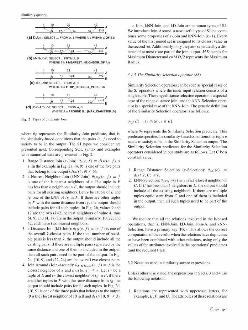
(a) -Join: SELECT … FROM A, B WHERE A.a WITHIN OF B.b

(d) Join-Around: SELECT … FROM A, B WHERE A.a AROUND B.b [MAX_DIAMETER 2r]

(c) kD-Join: SELECT ... FROM A, B WHERE A.a k TOP_CLOSEST_PAIRS B.b

N-Join: SELECT ... FROM A, B WHERE B.b k NEAREST_NEIGHBOR_OF A.a

4 10 22 42

9 17 24 39A

B

4 10 22 42

9 17 24 39A

Bk=2

4 10 22 42

9 17 24 39A

Bk=2

4 10 22 42

9 17 24 39A

Br = 3

=5

(b) kN

Fig. 2 Types of Similarity Join

where θS represents the Similarity Join predicate, that is,the similarity-based conditions that the pairs 〈e, f 〉 need tosatisfy to be in the output. The SJ types we consider arepresented next. Corresponding SQL syntax and exampleswith numerical data are presented in Fig. 2.

1. Range Distance Join (ε-Join): θε(e, f ) ≡ dist (e, f ) ≤ε. In the example in Fig. 2a, 〈4, 9〉 is one of the five pairsthat belong to the output (dist (4, 9) ≤ 5).

2. k Nearest Neighbor Join (kNN-Join): θk N N (e, f ) ≡ fis one of the k nearest neighbors of e. If a tuple in Ehas less than k neighbors in F , the output should includepairs for all existing neighbors. Let tE be a tuple of E andtF one of the kNN of tE in F . If there are other tuplesin F with the same distance from tE , the output shouldinclude pairs for all such tuples. In Fig. 2b, values 9 and17 are the two (k=2) nearest neighbors of value 4, thus〈4, 9〉 and 〈4, 17〉 are in the output. Similarly, 10, 22, and42, each have two nearest neighbors.

3. k-Distance Join (kD-Join): θk D(e, f ) ≡ 〈e, f 〉 is one ofthe overall k-closest pairs. If the total number of possi-ble pairs is less than k, the output should include all theexisting pairs. If there are multiple pairs separated by thesame distance and one of them is included in the output,then all such pairs need to be part of the output. In Fig.2c, 〈10, 9〉 and 〈22, 24〉 are the overall two closest pairs.

4. Join Around (Join-Around): θA,M D=2r (e, f ) ≡ f is theclosest neighbor of e and dist (e, f ) ≤ r . Let tE be atuple of E and tF the closest neighbor of tE in F , if thereare other tuples in F with the same distance from tE , theoutput should include pairs for all such tuples. In Fig. 2d,〈10, 9〉 is one of the three pairs that belongs to the output(9 is the closest neighbor of 10 in B and dist (10, 9) ≤ 3).

ε-Join, kNN-Join, and kD-Join are common types of SJ.We introduce Join-Around, a new useful type of SJ that com-bines some properties of ε-Join and kNN-Join (k=1). Everyvalue of the first joined set is assigned to its closest value inthe second set. Additionally, only the pairs separated by a dis-tance of at most r are part of the join output. M D stands forMaximum Diameter and r=M D/2 represents the MaximumRadius.

3.1.3 The Similarity Selection operator (SS)

Similarity Selection operators can be seen as special cases ofthe SJ operators where the inner input relation consists of asingle tuple. The range distance selection operator is a specialcase of the range distance join, and the kNN-Selection oper-ator is a special case of the kNN-Join. The generic definitionof the Similarity Selection operator is as follows:

σθS (E) = {e|θS(e), e ∈ E},

where θS represents the Similarity Selection predicate. Thispredicate specifies the similarity-based conditions that tuple eneeds to satisfy to be in the Similarity Selection output. TheSimilarity Selection predicates for the Similarity Selectionoperators considered in our study are as follows. Let C be aconstant value.

1. Range Distance Selection (ε-Selection): θε,C (e) ≡dist (e, C) ≤ ε.

2. kNN-Selection: θk N N ,C (e) ≡ e is a k-closest neighbor ofC . If C has less than k neighbors in E , the output shouldinclude all the existing neighbors. If there are multipletuples equidistant from C and one of them is includedin the output, then all such tuples need to be part of theoutput.

We require that all the relations involved in the k-basedoperations, that is, kNN-Join, kD-Join, Join-A, and kNN-Selection, have a primary key (PK). This allows the correctcomputation of the results when the relations have duplicatesor have been combined with other relations, using only thevalues of the attributes involved in the operations’ predicates(and the required PKs).

3.2 Notation used in similarity-aware expressions

Unless otherwise stated, the expressions in Sects. 3 and 4 usethe following notation:

1. Relations are represented with uppercase letters, forexample, E , F , and G. The attributes of these relations are

123

Y. N. Silva et al.

represented using the corresponding lowercase letters, forexample, e, f , and g. When an expression requires mul-tiple attributes of a given relation (E), we use a numbernext to the base name, for example, e1, e2, etc.

2. Similarity and regular (non-similarity) join predicates arespecified using the expression θS(e, f ). e and f are theouter and inner join attributes, respectively. When anexpression is applicable to multiple types of joins, thevalue of S is a general variable, for example, S, S1, orS2. If an expression is applicable to a particular typeof Similarity Join, the value of S can be: ε (ε-Join),k N N (kNN-Join), A (Join-Around), or k D (kD-Join).Regular join uses a similar notation without the compo-nent S. For example, the predicate θε(e, f ) representsan ε-Join between relations E (outer) and F (inner).E .e and F. f are the outer and inner join attributes,respectively.

3. Similarity and regular selection predicates are specifiedusing the expression θS,C (e). e is the selection attributeand C refers to the constant parameter in the case of SS.When an expression is applicable to multiple types ofselection, the value of S is a general variable, for exam-ple, S, S1, or S2. If an expression is applicable to a par-ticular type of Similarity Selection, the value of S can be:ε (ε-Selection) or k N N (kNN-Selection). Regular selec-tion predicates use the same notation without S and C .For example, the predicate θε 1,C1(e) represents anε-Selection operation that selects the tuples where thevalue of attribute E .e is within ε 1 of the constant C1.

4. Some generic rules have predicates that are applicableto both Similarity Selection and Similarity Join opera-tions. In this case, we use the notation θS, that can beinstantiated as θS,C (e) or θS(e, f ). Any constraints onthe operation attributes are directly specified on the rulesusing this notation.

5. As in regular relational algebra (RA), a (similarity) joinpredicate can be used with the selection or join oper-ators in similarity expressions. In regular RA: σθ(e, f )

(E × F) ≡ E ��θ(e, f ) F . Likewise, in similarity-awareRA: σθS(e, f )(E×F) ≡ E ��θS(e, f ) F . We use SimilarityJoin predicates with selection operators in rules that focuson the combination of multiple operations, for example,SS and SJ. The notation using a join operator is used inall other cases.

6. We say that the attributes of an expression have a sin-gle direction when the expression is composed by joinpredicates and their attribute graph is of the form a1 →a2 → · · · → an , for instance, e→ f → g. The attributegraph is built as follows. The vertices of the graph are thejoin attributes, and each join is represented as a directededge from the outer attribute (left attribute of the joinpredicate) to the inner one (right attribute of the joinpredicate).

E

S

S

,C1(e)

C1Output

kNN,C2(e)

C2

E

S,C1(e)

kNN,C2(e)

E

S

S ,C1(e)

C2Output

kNN,C2(e)

C1

kNN=4kNN=4

e ee

C1

C2

Evaluating

-Selection firstEvaluating

kNN-Selection first

kNN=4

Fig. 3 Different ways to combine ε-Selection and kNN-Selection

RegSelPred1 …RegSelPredp

EpsSelPred1 …EpsSelPredq

kNNSelPred1 …kNNSelPredr

RegJoinPred1 …RegJoinPreds

EpsJoinPred1 …EpsJoinPredt

kNNJoinPred1 …kNNJoinPredu

JoinArdPred1 …JoinArdPredv

kDJoinPred1 …kDJoinPredw

S

SGBRegGA1,…,RegGAx

SimGExp1,…,SimGExpy

E1 En...

SELECT [TOP k WITH TIES] ListOfAttributes FROM E1,…,En WHERERegSelPred1 AND…AND RegSelPredp ANDEpsSelPred1 AND…AND EpsSelPredq ANDkNNSelPred1 AND…AND kNNSelPredr ANDRegJoinPred1 AND…AND RegJoinPreds ANDEpsJoinPred1 AND…AND EpsJoinPredt ANDkNNJoinPred1 AND…AND kNNJoinPredu ANDJoinArdPred1 AND…AND JoinArdPredv ANDkDJoinPred1 AND…AND kDJoinPredw

GROUP BYRegGA1,…,RegGAx

SimGExp1,…,SimGExpy

ORDER BY SortExpr

TOP k

Fig. 4 Conceptual evaluation order of similarity queries

3.3 Conceptual evaluation order of similarity queries

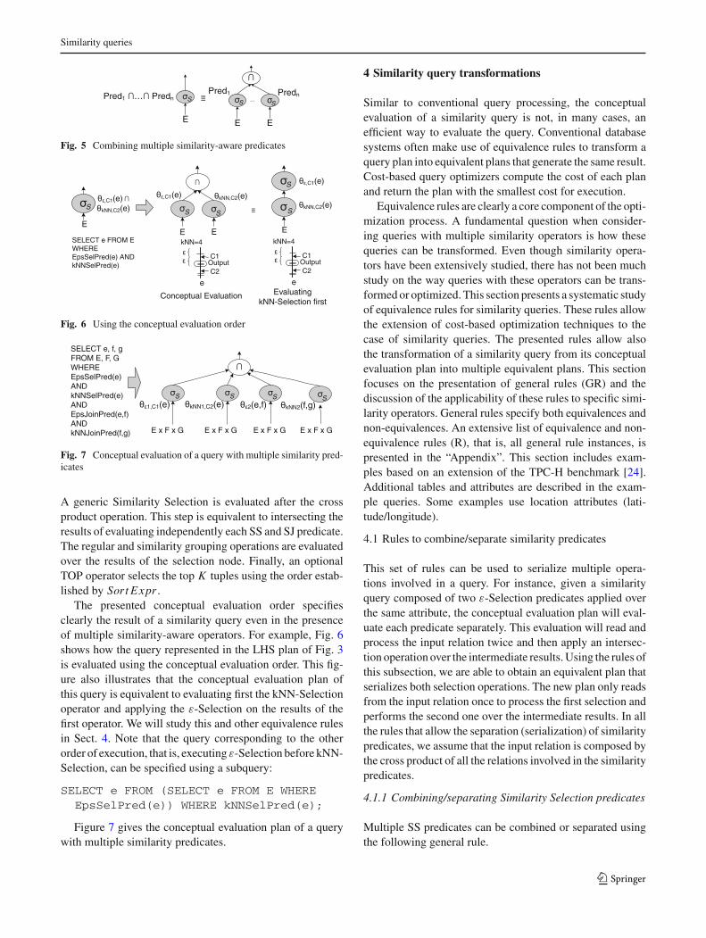
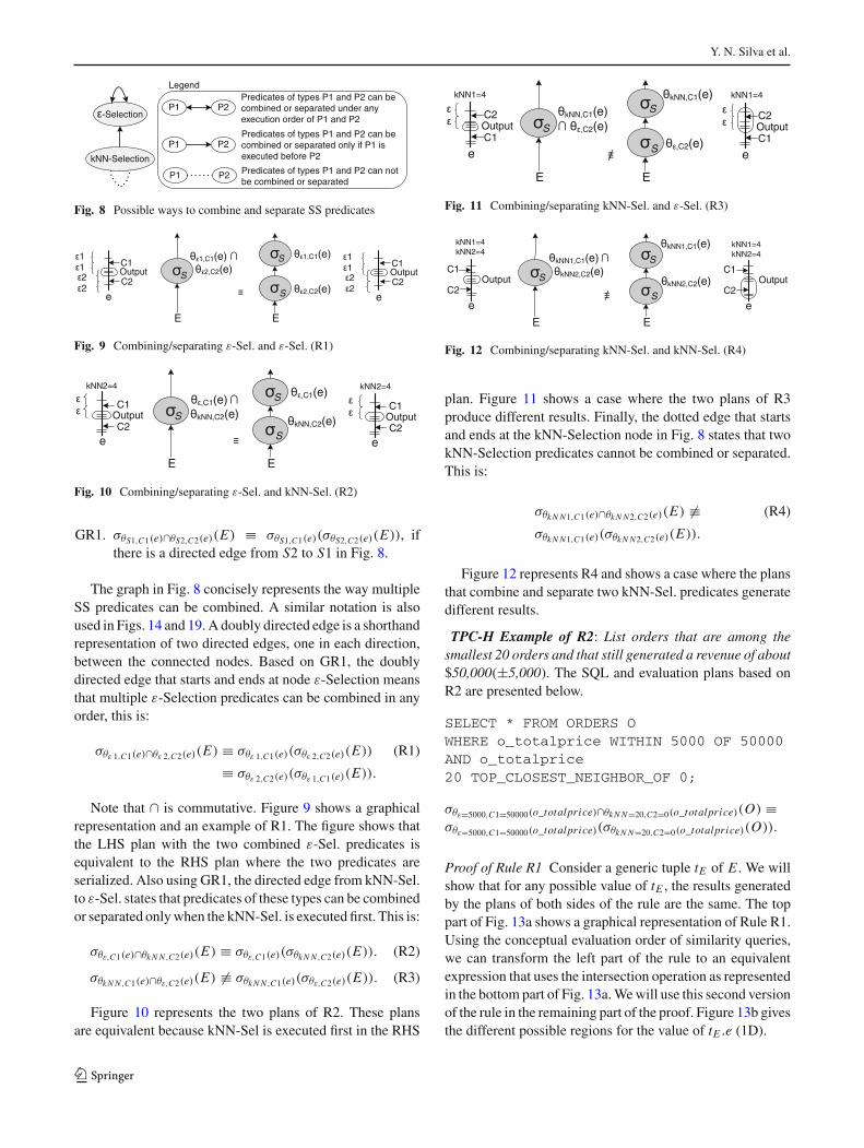
In general, the order in which the operations of a similarityquery are evaluated affects the results of a query. For instance,consider the left hand side (LHS) plan of Fig. 3. This planshows a similarity query with two Similarity Selection pred-icates (ε-Selection and kNN-Selection). Figure 3 illustratestwo ways in which this query could be evaluated and thedifferent results obtained under each evaluation. The middleplan in the figure corresponds to evaluating first the kNN-Selection predicate and applying the ε-Selection over theoutput of the first operator. The right-hand-side (RHS) plancorresponds to evaluating first the ε-Selection predicate andthen the kNN-Selection. It is not clear which way this queryshould be evaluated, and without a clear conceptual evalua-tion order of similarity queries, multiple users may write thesame query expecting different results.

Figure 4 presents the conceptual evaluation order for sim-ilarity queries. The conceptual query plan makes use of ageneric similarity-selection node that combines multiple SSand SJ predicates using the conventional intersection opera-tor as shown in Fig. 5. Based on the conceptual evaluationorder presented in Fig. 4, a generic similarity-aware querycomposed by multiple SGB, SJ, and SS operators is evalu-ated as follows. At the bottom of the plan, all the relationsinvolved in the query get combined using cross product.

123

Similarity queries

Pred1 … Predn S

E

S

E

Pred1...

S

Predn

E

Fig. 5 Combining multiple similarity-aware predicates

C1OutputC2

E

S,C1(e)

kNN,C2(e)

kNN=4

eEvaluating

kNN-Selection first

S S

E E

,C1(e) kNN,C2(e)

E

S

S

,C1(e)

kNN,C2(e)

Conceptual Evaluation

C1OutputC2

kNN=4

e

SELECT e FROM EWHEREEpsSelPred(e) ANDkNNSelPred(e)

Fig. 6 Using the conceptual evaluation order

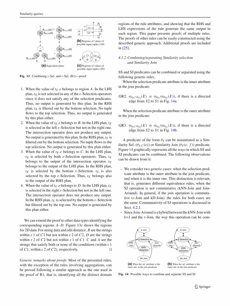
SELECT e, f, g FROM E, F, GWHEREEpsSelPred(e)ANDkNNSelPred(e)ANDEpsJoinPred(e,f)ANDkNNJoinPred(f,g)

S S1,C1(e) kNN1,C2(e)

S S

E x F x G E x F x G E x F x G E x F x G

kNN2(f,g)2(e,f)

Fig. 7 Conceptual evaluation of a query with multiple similarity pred-icates

A generic Similarity Selection is evaluated after the crossproduct operation. This step is equivalent to intersecting theresults of evaluating independently each SS and SJ predicate.The regular and similarity grouping operations are evaluatedover the results of the selection node. Finally, an optionalTOP operator selects the top K tuples using the order estab-lished by Sort Expr .

The presented conceptual evaluation order specifiesclearly the result of a similarity query even in the presenceof multiple similarity-aware operators. For example, Fig. 6shows how the query represented in the LHS plan of Fig. 3is evaluated using the conceptual evaluation order. This fig-ure also illustrates that the conceptual evaluation plan ofthis query is equivalent to evaluating first the kNN-Selectionoperator and applying the ε-Selection on the results of thefirst operator. We will study this and other equivalence rulesin Sect. 4. Note that the query corresponding to the otherorder of execution, that is, executing ε-Selection before kNN-Selection, can be specified using a subquery:

SELECT e FROM (SELECT e FROM E WHEREEpsSelPred(e)) WHERE kNNSelPred(e);

Figure 7 gives the conceptual evaluation plan of a querywith multiple similarity predicates.

4 Similarity query transformations

Similar to conventional query processing, the conceptualevaluation of a similarity query is not, in many cases, anefficient way to evaluate the query. Conventional databasesystems often make use of equivalence rules to transform aquery plan into equivalent plans that generate the same result.Cost-based query optimizers compute the cost of each planand return the plan with the smallest cost for execution.

Equivalence rules are clearly a core component of the opti-mization process. A fundamental question when consider-ing queries with multiple similarity operators is how thesequeries can be transformed. Even though similarity opera-tors have been extensively studied, there has not been muchstudy on the way queries with these operators can be trans-formed or optimized. This section presents a systematic studyof equivalence rules for similarity queries. These rules allowthe extension of cost-based optimization techniques to thecase of similarity queries. The presented rules allow alsothe transformation of a similarity query from its conceptualevaluation plan into multiple equivalent plans. This sectionfocuses on the presentation of general rules (GR) and thediscussion of the applicability of these rules to specific simi-larity operators. General rules specify both equivalences andnon-equivalences. An extensive list of equivalence and non-equivalence rules (R), that is, all general rule instances, ispresented in the “Appendix”. This section includes exam-ples based on an extension of the TPC-H benchmark [24].Additional tables and attributes are described in the exam-ple queries. Some examples use location attributes (lati-tude/longitude).

4.1 Rules to combine/separate similarity predicates

This set of rules can be used to serialize multiple opera-tions involved in a query. For instance, given a similarityquery composed of two ε-Selection predicates applied overthe same attribute, the conceptual evaluation plan will eval-uate each predicate separately. This evaluation will read andprocess the input relation twice and then apply an intersec-tion operation over the intermediate results. Using the rules ofthis subsection, we are able to obtain an equivalent plan thatserializes both selection operations. The new plan only readsfrom the input relation once to process the first selection andperforms the second one over the intermediate results. In allthe rules that allow the separation (serialization) of similaritypredicates, we assume that the input relation is composed bythe cross product of all the relations involved in the similaritypredicates.

4.1.1 Combining/separating Similarity Selection predicates

Multiple SS predicates can be combined or separated usingthe following general rule.

123

Y. N. Silva et al.

-Selection

Legend

P1 P2

P1 P2

P1 P2

Predicates of types P1 and P2 can be combined or separated under any execution order of P1 and P2

Predicates of types P1 and P2 can be combined or separated only if P1 is executed before P2

Predicates of types P1 and P2 can not be combined or separated

kNN-Selection

Fig. 8 Possible ways to combine and separate SS predicates

E

S

S

1,C1(e)C11

1

Output

2,C2(e)C2

22

E

S

1,C1(e)2,C2(e)Output

C1

C2

11

22

e e

Fig. 9 Combining/separating ε-Sel. and ε-Sel. (R1)

E

S

S

,C1(e)C1

OutputkNN,C2(e)

C2

E

S,C1(e)

kNN,C2(e)OutputC1

C2

kNN2=4

e e

kNN2=4

Fig. 10 Combining/separating ε-Sel. and kNN-Sel. (R2)

GR1. σθS1,C1(e)∩θS2,C2(e)(E) ≡ σθS1,C1(e)(σθS2,C2(e)(E)), ifthere is a directed edge from S2 to S1 in Fig. 8.

The graph in Fig. 8 concisely represents the way multipleSS predicates can be combined. A similar notation is alsoused in Figs. 14 and 19. A doubly directed edge is a shorthandrepresentation of two directed edges, one in each direction,between the connected nodes. Based on GR1, the doublydirected edge that starts and ends at node ε-Selection meansthat multiple ε-Selection predicates can be combined in anyorder, this is:

σθε 1,C1(e)∩θε 2,C2(e)(E) ≡ σθε 1,C1(e)(σθε 2,C2(e)(E)) (R1)

≡ σθε 2,C2(e)(σθε 1,C1(e)(E)).

Note that ∩ is commutative. Figure 9 shows a graphicalrepresentation and an example of R1. The figure shows thatthe LHS plan with the two combined ε-Sel. predicates isequivalent to the RHS plan where the two predicates areserialized. Also using GR1, the directed edge from kNN-Sel.to ε-Sel. states that predicates of these types can be combinedor separated only when the kNN-Sel. is executed first. This is:

σθε,C1(e)∩θk N N ,C2(e)(E) ≡ σθε,C1(e)(σθk N N ,C2(e)(E)). (R2)

σθk N N ,C1(e)∩θε,C2(e)(E) �≡ σθk N N ,C1(e)(σθε,C2(e)(E)). (R3)

Figure 10 represents the two plans of R2. These plansare equivalent because kNN-Sel is executed first in the RHS

E

S

S ,C2(e)

C2Output

kNN,C1(e)

C1

E

SkNN,C1(e)

,C2(e)C2OutputC1

kNN1=4

e e

kNN1=4

Fig. 11 Combining/separating kNN-Sel. and ε-Sel. (R3)

E

S

S

C1OutputkNN2,C2(e)

C2

E

S

kNN1,C1(e)kNN2,C2(e)

kNN1,C1(e)

C1Output

C2

kNN1=4kNN2=4

e e

kNN1=4kNN2=4

Fig. 12 Combining/separating kNN-Sel. and kNN-Sel. (R4)

plan. Figure 11 shows a case where the two plans of R3produce different results. Finally, the dotted edge that startsand ends at the kNN-Selection node in Fig. 8 states that twokNN-Selection predicates cannot be combined or separated.This is:

σθk N N1,C1(e)∩θk N N2,C2(e)(E) �≡ (R4)

σθk N N1,C1(e)(σθk N N2,C2(e)(E)).

Figure 12 represents R4 and shows a case where the plansthat combine and separate two kNN-Sel. predicates generatedifferent results.

TPC-H Example of R2: List orders that are among thesmallest 20 orders and that still generated a revenue of about$50,000(±5,000). The SQL and evaluation plans based onR2 are presented below.

SELECT * FROM ORDERS OWHERE o_totalprice WITHIN 5000 OF 50000AND o_totalprice20 TOP_CLOSEST_NEIGHBOR_OF 0;

σθε=5000,C1=50000(o_totalprice)∩θk N N=20,C2=0(o_totalprice)(O) ≡σθε=5000,C1=50000(o_totalprice)(σθk N N=20,C2=0(o_totalprice)(O)).

Proof of Rule R1 Consider a generic tuple tE of E . We willshow that for any possible value of tE , the results generatedby the plans of both sides of the rule are the same. The toppart of Fig. 13a shows a graphical representation of Rule R1.Using the conceptual evaluation order of similarity queries,we can transform the left part of the rule to an equivalentexpression that uses the intersection operation as representedin the bottom part of Fig. 13a. We will use this second versionof the rule in the remaining part of the proof. Figure 13b givesthe different possible regions for the value of tE .e (1D).

123

Similarity queries

e

1

1

A

A

B

S S

E E

C1

C222 D

C

E

S

S

1,C1(e)

2,C2(e)

E

S

1,C1(e)2,C2(e)

E

S

S

1,C1(e)

2,C2(e)1,C1(e) 2,C2(e)

(a) Equivalent plans

(b) Regions of values ofpossible input tuples (1D)

(c) Regions of values ofpossible input tuples (2D)

1 2

A BC

D

C1 C2

Fig. 13 Combining ε-Sel. and ε-Sel. (R1)—proof

1. When the value of tE .e belongs to region A. In the LHSplan, tE is not selected in any of the ε-Selection operatorssince it does not satisfy any of the selection predicates.Thus, no output is generated by this plan. In the RHSplan, tE is filtered out by the bottom selection. No tupleflows to the top selection. Thus, no output is generatedby this plan either.

2. When the value of tE .e belongs to B. In the LHS plan, tE

is selected in the left ε-Selection but not in the right one.The intersection operator does not produce any output.No output is generated by this plan. In the RHS plan, tE isfiltered out by the bottom selection. No tuple flows to thetop selection. No output is generated by this plan either.

3. When the value of tE .e belongs to C . In the LHS plan,tE is selected by both ε-Selection operators. Thus, tE

belongs to the output of the intersection operator. tE

belongs to the output of the LHS plan. In the RHS plan,tE is selected by the bottom ε-Selection. tE is alsoselected by the top ε-Selection. Thus, tE belongs alsoto the output of the RHS plan.

4. When the value of tE .e belongs to D. In the LHS plan, tE

is selected in the right ε-Selection but not in the left one.The intersection operator does not produce any output.In the RHS plan, tE is selected by the bottom ε-Selectionbut filtered out by the top one. No output is generated bythis plan either.

We can extend the proof to other data types identifying thecorresponding regions A–D. Figure 13c shows the regionsfor 2D data. For string data and edit distance, B are the stringswithin ε 1 of C1 but not within ε 2 of C2, D are the stringswithin ε 2 of C2 but not within ε 1 of C1. C and A are thestrings that satisfy both or none of the conditions (within ε 1of C1, within ε 2 of C2), respectively. �

Generic remarks about proofs Most of the presented rules,with the exception of the rules involving aggregations, canbe proved following a similar approach as the one used inthe proof of R1, that is, identifying all the distinct domain

regions of the rule attributes, and showing that the RHS andLHS expressions of the rule generate the same output ineach region. This paper presents proofs of multiple rules.The proofs of other rules can be easily constructed using thedescribed generic approach. Additional proofs are includedin [25].

4.1.2 Combining/separating Similarity selectionand Similarity Join

SS and SJ predicates can be combined or separated using thefollowing generic rules.

When the selection predicate attribute is the inner attributein the join predicate:

GR2. σθS1∩θS2(E) ≡ σθS1(σθS2(E)), if there is a directededge from S2 to S1 in Fig. 14a.

When the selection predicate attribute is the outer attributein the join predicate:

GR3. σθS1∩θS2(E) ≡ σθS1(σθS2(E)), if there is a directededge from S2 to S1 in Fig. 14b.

A predicate of the form θS can be instantiated as a Sim-ilarity Sel. (θS,C (e)) or Similarity Join (θS(e, f )) predicate.Figure 14 graphically represents all the ways in which SS andSJ predicates can be combined. The following observationscan be drawn from it:

– We consider two generic cases: when the selection pred-icate attribute is the outer attribute in the join predicate,and when it is the inner one. This distinction is relevant,that is, generates different equivalence rules, when theSJ operation is not commutative (kNN-Join and Join-Around). In general, if the join operation is commuta-tive (ε-Join and kD-Join), the rules for both cases arethe same. Commutativity of SJ operations is discussed inSect. 4.2.1.

– Since Join-Around is a hybrid between the kNN-Join withk=1 and the ε-Join, the way this operation can be com-

-Join

kNN-Join

Join-Around

kD-Join

-Selection

kNN-Selection

-Join

kNN-Join

Join-Around

kD-Join

-Selection

kNN-Selection

(a) When the sel. attribute is theinner attr. in the join predicate

(b) When the sel. attribute is theouter attr. in the join predicate

Fig. 14 Possible ways to combine and separate SS and SJ

123

Y. N. Silva et al.

E

1(e1,e2)2,C(e2)

S

S

e1 e2

C

E

2,C(e2)S

1(e1,e2)S

E

2,C(e2)

S 1(e1,e2)

22

Output

1e1 e2

C22

Output

1e1 e2

C22

Output

1

Fig. 15 Combining/separating ε-Join and ε-Sel. (R5)

bined with a given SS operator corresponds to the mostrestricted way in which the kNN-Join or the ε-Join can becombined with that SS operator. This observation appliesin fact to any rule that uses Join-Around.

– The rules where the selection attribute is the inner joinattribute (Fig. 14a) are equal to or more restrictive thanthe corresponding rules where the selection attribute isthe outer join attribute (Fig. 14b).

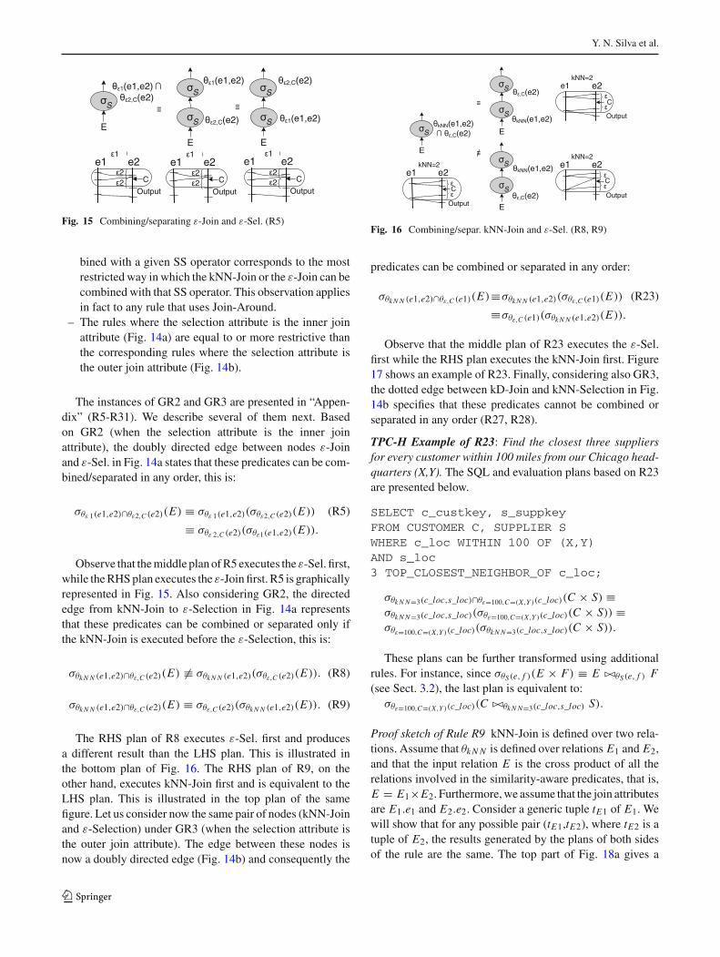
The instances of GR2 and GR3 are presented in “Appen-dix” (R5-R31). We describe several of them next. Basedon GR2 (when the selection attribute is the inner joinattribute), the doubly directed edge between nodes ε-Joinand ε-Sel. in Fig. 14a states that these predicates can be com-bined/separated in any order, this is:

σθε 1(e1,e2)∩θε2,C (e2)(E) ≡ σθε 1(e1,e2)(σθε2,C (e2)(E)) (R5)

≡ σθε 2,C (e2)(σθε1(e1,e2)(E)).

Observe that the middle plan of R5 executes the ε-Sel. first,while the RHS plan executes the ε-Join first. R5 is graphicallyrepresented in Fig. 15. Also considering GR2, the directededge from kNN-Join to ε-Selection in Fig. 14a representsthat these predicates can be combined or separated only ifthe kNN-Join is executed before the ε-Selection, this is:

σθk N N (e1,e2)∩θε,C (e2)(E) �≡ σθk N N (e1,e2)(σθε,C (e2)(E)). (R8)

σθk N N (e1,e2)∩θε,C (e2)(E) ≡ σθε,C (e2)(σθk N N (e1,e2)(E)). (R9)

The RHS plan of R8 executes ε-Sel. first and producesa different result than the LHS plan. This is illustrated inthe bottom plan of Fig. 16. The RHS plan of R9, on theother hand, executes kNN-Join first and is equivalent to theLHS plan. This is illustrated in the top plan of the samefigure. Let us consider now the same pair of nodes (kNN-Joinand ε-Selection) under GR3 (when the selection attribute isthe outer join attribute). The edge between these nodes isnow a doubly directed edge (Fig. 14b) and consequently the

E

kNN(e1,e2),C(e2)S

S

EkNN(e1,e2)

S

,C(e2)

S

E

S

e1 e2

C

Output

kNN=2kNN(e1,e2)

,C(e2)

e1 e2

C

Output

kNN=2

e1 e2

C

Output

kNN=2

Fig. 16 Combining/separ. kNN-Join and ε-Sel. (R8, R9)

predicates can be combined or separated in any order:

σθk N N (e1,e2)∩θε,C (e1)(E)≡σθk N N (e1,e2)(σθε,C (e1)(E)) (R23)

≡σθε,C (e1)(σθk N N (e1,e2)(E)).

Observe that the middle plan of R23 executes the ε-Sel.first while the RHS plan executes the kNN-Join first. Figure17 shows an example of R23. Finally, considering also GR3,the dotted edge between kD-Join and kNN-Selection in Fig.14b specifies that these predicates cannot be combined orseparated in any order (R27, R28).

TPC-H Example of R23: Find the closest three suppliersfor every customer within 100 miles from our Chicago head-quarters (X,Y). The SQL and evaluation plans based on R23are presented below.

SELECT c_custkey, s_suppkeyFROM CUSTOMER C, SUPPLIER SWHERE c_loc WITHIN 100 OF (X,Y)AND s_loc3 TOP_CLOSEST_NEIGHBOR_OF c_loc;

σθk N N=3(c_loc,s_loc)∩θε=100,C=(X,Y )(c_loc)(C × S) ≡σθk N N=3(c_loc,s_loc)(σθε=100,C=(X,Y )(c_loc)(C × S)) ≡σθε=100,C=(X,Y )(c_loc)(σθk N N=3(c_loc,s_loc)(C × S)).

These plans can be further transformed using additionalrules. For instance, since σθS(e, f )(E × F) ≡ E ��θS(e, f ) F(see Sect. 3.2), the last plan is equivalent to:

σθε=100,C=(X,Y )(c_loc)(C ��θk N N=3(c_loc,s_loc) S).

Proof sketch of Rule R9 kNN-Join is defined over two rela-tions. Assume that θk N N is defined over relations E1 and E2,and that the input relation E is the cross product of all therelations involved in the similarity-aware predicates, that is,E = E1×E2. Furthermore, we assume that the join attributesare E1.e1 and E2.e2. Consider a generic tuple tE1 of E1. Wewill show that for any possible pair (tE1,tE2), where tE2 is atuple of E2, the results generated by the plans of both sidesof the rule are the same. The top part of Fig. 18a gives a

123

Similarity queries

E

kNN(e1,e2),C(e1)S

S

E

kNN(e1,e2)

S ,C(e1)

S

E

S

e2e1

COutput

kNN=2

kNN(e1,e2)

,C(e1)

e2e1

COutput

kNN=2e2e1

COutput

kNN=2

Fig. 17 Combining/separating kNN-Join and ε-Sel. (R23)

E

kNN(e1,e2),C(e2) S

S

E

kNN(e1,e2)S

,C(e2)

S

E

kNN(e1,e2)S

,C(e2)

S S

E E

,C(e2)kNN(e1,e2)

e2

C

e1

kNN

A

A

B

D

M

tE1

tE2

(a) Equivalent plans(b) Regions of values of

possible input tuples

Fig. 18 Combining kNN-Join and ε-Sel. (R9)—proof

graphical representation of Rule R9. Using the conceptualevaluation order of similarity queries, we can transform theleft part of the rule to an equivalent expression that uses theintersection operation as represented in the bottom part ofFig. 18a. We will use this version of the rule in the remain-ing part of the proof. Figure 18b gives the different possibleregions for the value of tE2.e2. Note that the region markedas kNN (which comprises regions B and M) represents theregion that contains the kNN closest neighbors of tE1 in E2.

1. When the value of tE2.e2 belongs to A. In the LHS plan,(tE1,tE2) is not selected in any of the operators. No outputis generated by this plan. In the RHS plan, (tE1,tE2) isfiltered out by the bottom selection since tE2 is not one ofthe kNN closest neighbors of tE1 in E2. No tuple flows tothe top operator and no output is generated by this plan.

2. When the value of tE2.e2 belongs to B. In the LHS plan,the pair (tE1,tE2) is selected in the left operator but notin the right one. The intersection operator does not pro-duce any output and consequently no output is generatedby this plan. In the RHS plan, (tE1,tE2) is selected inthe bottom selection since tE2 is one of the kNN closestneighbors of tE1 in E2. However, (tE1,tE2) is filtered outby the top selection because dist (tE2.e2, C) > ε. Thus,no output is generated by this plan either.

3. When the value of tE2.e2 belongs to M . In the LHS plan,(tE1,tE2) is selected in both operators. Consequently,(tE1,tE2) belongs to the output of the intersection andthe LHS plan. In the RHS plan, (tE1,tE2) is selected bythe bottom selection since tE2 is one of the kNN closest

neighbors of tE1 in E2. (tE1,tE2) is also selected by thetop selection since dist (tE2.e2, C) ≤ ε. Thus, (tE1,tE2)belongs also to the output of the RHS plan.

4. When the value of tE2.e2 belongs to D. In the LHS plan,the pair (tE1,tE2) is selected in the right similarity opera-tor but not in the left one. The intersection operator doesnot produce any output and thus no output is generatedby this plan. In the RHS plan, (tE1,tE2) is filtered out bythe bottom selection. No tuple flows to the top operator.Thus, no output is generated by this plan either. �

4.1.3 Combining/separating Similarity Join predicates

Multiple SJ predicates can be combined or separated usingthe following general rules.

When the attributes in the predicates have a single direc-tion (e1→ e2, e2→ e3):

GR4. σθS1(e1,e2)∩θS2(e2,e3)(E) ≡ σθS1(e1,e2)(σθS2(e2,e3)(E)),and σθS1(e1,e2)∩θS2(e2,e3)(E) ≡ σθS2(e2,e3)(σθS1(e1,e2)

(E)), if the graph of Fig. 19a has a doubly directed

edge of the form: S1(e1,e2)←−−−−(e2,e3)−−−−→ S2.

GR5. σθS1(e1,e2)∩θS2(e2,e3)(E) ≡ σθS1(e1,e2)(σθS2(e2,e3)(E)),and σθS1(e1,e2)∩θS2(e2,e3)(E) �≡ σθS2(e2,e3)(σθS1(e1,e2)

(E)), if the graph of Fig. 19a has a directed edge of

the form: S1(e1,e2) (e2,e3)←−−−−−−−− S2.

When the attributes in the predicates do not have a singledirection (e1→ e2, e2← e3):

GR6. σθS1(e1,e2)∩θS2(e3,e2)(E) ≡ σθS1(e1,e2)(σθS2(e3,e2)(E)),and σθS1(e1,e2)∩θS2(e3,e2)(E) ≡ σθS2(e3,e2)(σθS1(e1,e2)

(E)), if the graph of Fig. 19b has a doubly directed

edge of the form: S1(e1,e2)←−−−−(e3,e2)−−−−→ S2.

GR7. σθS1(e1,e2)∩θS2(e3,e2)(E) ≡ σθS1(e1,e2)(σθS2(e3,e2)(E)),and σθS1(e1,e2)∩θS2(e3,e2)(E) �≡ σθS2(e3,e2)(σθS1(e1,e2)

-Join

kNN-Join

Join-Around

kD-Join

(e1,e2)(e1,e2)(e2,e3)

(e2,e3)(e2,

e3)

(e1,

e2)

(e1,e2)

(e2,

e3)(e2,e3)

(e1,

e2)

(e2,e3) (e1,e2)

-Join

kNN-Join

Join-Around

kD-Join

(e1,e2)(e1,e2)(e2,e3)

(e2,e3)(e2,

e3)

(e1,

e2)

(e1,e2)

(e2,

e3)(e2,e3)

(e1,

e2)

(e2,e3) (e1,e2)

(a) When the attributes in the predicates have a single direction: e1 e2, e2 e3

(b) When the attributes in the predicates do not have a single direction: e1 e2, e2 e3

Fig. 19 Possible ways to combine/separate SJ predicates

123

Y. N. Silva et al.

E

1(e1,e2)2(e2,e3)S

S

e1 e2E

2(e2,e3)S

1(e1,e2)S

E

2(e2,e3)

S 1(e1,e2)

Output

e3 e1 e2

Output

e3 e1 e2

Output

e3

Fig. 20 Combining/separating two ε-Join predicates (R32)

(E)), if the graph of Fig. 19b has a directed edge of

the form: S1(e1,e2) (e3,e2)←−−−−−−−− S2.

If the edge between two nodes is dotted in Fig. 19, noneof the equivalences presented in rules GR4 or GR6 hold. Thegraphs in Fig. 19 show the different ways in which two SJpredicates can be combined/separated. Two cases are con-sidered: when the attributes in the predicates have a singledirection, for example, e1→ e2, e2→ e3; and when this isnot the case, for example, e1→ e2, e2← e3. In general, thisclassification generates different equivalence rules when atleast one of the SJ operations is not commutative (kNN-Joinand Join-Around). The “Appendix” presents all the instancesof GR4-GR7 (R32-R65). We describe some of these here.

Under GR4 (predicates’ attributes have a single direction:e1→ e2, e2→ e3), the doubly directed edge that starts andends at the ε-Join node in Fig. 19a specifies that two ε-Joinpredicates can be combined in any order. This is:

σθε 1(e1,e2)∩θε 2(e2,e3)(E)≡σθε 1(e1,e2)(σθε 2(e2,e3)(E)) (R32)

≡σθε 2(e2,e3)(σθε 1(e1,e2)(E)).

Rule R32 is presented graphically in Fig. 20.Under GR7 (predicates’ attributes do not have a single

direction: e1→ e2, e2← e3), the directed edge from kNN-Join to ε-Join in Fig. 19b states that these predicates can be

combined executing kNN-Join first:

σθε(e1,e2)∩θk N N (e3,e2)(E) ≡ σθε(e1,e2)(σθk N N (e3,e2)(E)).

(R52)

σθε(e1,e2)∩θk N N (e3,e2)(E) �≡ σθk N N (e3,e2)(σθε(e1,e2)(E)).

(R53)

kNN-Join is executed first in the RHS plan of R52 whileε-Join is executed first in the RHS plan of R53.

4.2 Other core equivalence rules

4.2.1 Commutativity of Similarity Join operators

Some SJ operations (ε-Join and kD-Join) are commutativeas specified by the following general rule.

GR8. E ��θS(e, f ) F ≡ F ��θS(e, f ) E , when (i) S is ε-Join orkD-Join but not kNN-Join or Join-Around, and (ii) thedistance function used in the operations is symmetric.

4.2.2 Distribution of (similarity or regular) selection over(similarity or regular) join

Pushing selection below join (distributing selection over join)is one of the most useful rules in regular relational algebra.In this section, we extend this rule to the case of SS andSJ. Similarity or regular selection operations can be pushedbelow similarity or regular join operations according to thefollowing general rules.

When the selection predicate attribute is the outer attributein the join predicate:GR9. σθS1(e)(E ��θS2(e, f ) F) ≡ (σθS1(e)(E)) ��θS2(e, f ) F ,

if cell [S1, S2] in Table 1a is checked.

When the selection predicate attribute is the inner attributein the join predicate:GR10. σθS1( f )(E ��θS2(e, f ) F) ≡ E ��θS2(e, f ) (σθS1( f )

(F)), if cell [S1, S2] in Table 1b is checked.

Table 1 Cases where selection can be pushed below join

Reg. Join ε-Join kNN-Join kD-Join Join-Around

(a) When the selection predicate attribute is the outer attribute in the join predicate

Reg. Selection � � � �ε-Selection � � � �kNN-Selection �

(b) When the selection predicate attribute is the inner attribute in the join predicate

Reg. Selection � �ε-Selection � �kNN-Selection

123

Similarity queries

E

S

F E

S

F

(e)

(e,f)

(e,f)

(e)

fA

e

a2

A

B

a1

tE tF

(a) Equivalent plans(b) Regions of values of

possible input tuples

Fig. 21 Distribution of selection over ε-Join (R70)

Table 1 summarizes all the cases where a selection opera-tor (regular or similarity-aware) can be pushed below a join(regular or similarity-aware). This table and general rulesGR9 and GR10 consider two generic cases: when the selec-tion attribute is the outer attribute of the join predicate andwhen it is the inner one. The instances of GR9 and GR10(R70-R101) are included in the “Appendix”. Some of themare presented next.

In some cases, a given selection type can be pushed beloweither input of a join. For instance, this is the case for regularselection and ε-Join. Note that both cells [Regular Selection,ε-Join] in Table 1a and b have a check mark. Using GR9 andGR10 we obtain:

σθ(e)(E ��θε(e, f ) F) ≡ (σθ(e)(E)) ��θε(e, f ) F. (R70)

σθ( f )(E ��θε(e, f ) F) ≡ E ��θε(e, f ) (σθ( f )(F)). (R71)

In R70, selection is pushed below the outer input of ε-Join;in R70, below the inner one. Figure 21a represents Rule R70graphically. Similarly, for the case of ε-Selection and ε-Joinwe have:

σθε 1,C (e)(E ��θε 2(e, f ) F) ≡ (σθε 1,C (e)(E)) ��θε 2(e, f ) F.

(R86)

σθε 1,C ( f )(E ��θε 2(e, f ) F) ≡ E ��θε 2(e, f ) (σθε 1,C ( f )(F)).

(R87)

In other cases, selection can only be pushed below theouter input of a join. This is the case for ε-Join and kNN-Join. Note that the cell [Regular Selection, ε-Join] has a checkmark only in Table 1a. Using GR9 and GR10, we get thefollowing rules:

σθε,C (e)(E ��θk N N (e, f ) F) ≡ (σθε,C (e)(E)) ��θk N N (e, f ) F.

(R88)

σθε,C ( f )(E ��θk N N (e, f ) F) �≡ E ��θk N N (e, f ) (σθε,C ( f )(F)).

(R89)

Figure 22 shows that pushing ε-Sel. below the outer inputof kNN-Join generates the same result as executing kNN-Join first. On the other hand, pushing ε-Sel. below the innerinput of kNN-Join can generate a different result as seen inFig. 23.

E F E F

S

SS

S

C Output OutputC

,C(e)

,C(e)

kNN(e,f)

kNN(e,f)kNN=2 kNN=2

e f e f

Fig. 22 Distribution of ε-Sel. over kNN-Join—when sel. is pushedbelow the outer relation (R88)

E F E F

S

S

SkNN=2

C

Output

S

C

Output,C(f)

,C(f)

kNN(e,f)

kNN(e,f)kNN=2

e f e f

Fig. 23 Distribution of ε-Sel. over kNN-Join—when sel. is pushedbelow the inner relation (R89)

TPC-H Example of R86: Considering the customers thatare located within 200 miles from our Chicago headquarters(X,Y), identify the customers that are located within 10 milesof certain locations of interest (INTER_ LOCATION). TheSQL and evaluation plans based on R86 are presented below.

SELECT c_custkey, il_locNameFROM CUSTOMER C, INTER_LOCATION ILWHERE c_loc WITHIN 10 OF il_loc AND

c_loc WITHIN 200 OF (X,Y);

σθε 1=200,C=(X,Y )(c_loc)(C ��θε 2=10(c_loc,il_loc) I L) ≡(σθε 1=200,C=(X,Y )(c_loc)(C)) ��θε 2=10(c_loc,il_loc) I L .

Proof sketch of Rule R70 The join attributes in θε are E .eand F. f , and θ is defined over E .e. Consider a generic tupletE of E . We will show that for any possible pair (tE ,tF ),where tF is a tuple of F , the results generated by the plansof both sides of the rule are the same. Figure 21b gives thedifferent possible regions for the values of tF . f , and twogeneric values of tE .e. a2 represent a value that satisfies thepredicate θ while a1 represents a value that does not.

1. When the value of tE .e is a1. In the LHS plan, the pair(tE ,tF ) may or may not belong to the output of the ε-Join. However, (tE ,tF ) will be filtered out by the selectionoperator since a1 does not satisfy the predicate θ . Thus,no output is generated by this plan. In the RHS plan, tE

is filtered out by the selection since a1 does not satisfy θ .No tuple flows to the ε-Join operator from its outer input.Thus, no output is generated by this plan either.

2. When the value of tE .e is a2 and the value of tF . f belongsto A. In the LHS plan, the pair (tE ,tF ) does not belong tothe output of the ε-Join since dist (tE .e, tF . f ) > ε. Notuple flows to the selection operator. Thus, no output isgenerated by this plan. In the RHS plan, tE is selected by

123

Y. N. Silva et al.

the regular selection operator since a2 satisfies θ . How-ever, the pair (tE ,tF ) does not belong to the output ofthe ε-Join since dist (tE .e, tF . f ) > ε. Thus, no output isgenerated by this plan either.

3. When tE .e is a2 and the value of tF . f belongs to B.In the LHS plan, the pair (tE ,tF ) belongs to the out-put of the ε-Join since dist (tE .e, tF . f ) ≤ ε. (tE ,tF ) isalso selected by the regular operator since a2 satisfies θ .(tE ,tF ) belongs to the output of this plan. In the RHSplan, tE is selected by the selection operator since a2 sat-isfies θ . (tE ,tF ) belongs to the output of the ε-Join sincedist (tE .e, tF . f ) ≤ ε. Thus, (tE ,tF ) also belongs to theoutput of this plan. �

4.2.3 Associativity of Similarity Join operators

Associativity of join operators is another core transforma-tion rule commonly used in query optimization. This ruleallows re-ordering multiple join operations and can signif-icantly improve the efficiency of a query because differentorders can generate different sizes of the intermediate results.In general, plans with smaller intermediate results are alsomore efficient. SJ operations are associative according to thefollowing general rules.

When the attributes in the predicates have a single direc-tion (e→ f , f → g):GR11. (E ��θS1(e, f ) F) ��θS2( f,g) G ≡ E ��θS1(e, f )

(F ��θS2( f,g) G), when S1 and S2 are both: ε-Join,kNN-Join, or Join-Around but not kD-Join.

When the predicates’ attributes do not have a single direc-tion (e→ f , f ← g):GR12. G ��θS1(g, f ) (E ��θS2(e, f ) F) ≡ E ��θS2(e, f )

(G ��θS1(g, f ) F), when S1 and S2 are both: ε-Joinbut not kNN-Join, kD-Join or Join-Around.

The associativity of multiple SJ operators depends in gen-eral on whether or not the predicates’ attributes have a singledirection. This distinction, however, is not relevant (generatethe same rules) when the join operators are commutative (ε-Join and kD-Join). All the instances of GR11 and GR12 arepresented in the “Appendix” (R102 to R109). We describehere some of them.

In the case of a query with two ε-Join operations, basedon GR11 and GR12, we can re-order the operations whetherthe attributes in the predicates have a single direction or not.The corresponding rule instances are:

(E ��θε 1(e, f ) F) ��θε 2( f,g) G ≡ (R102)

E ��θε 1(e, f ) (F ��θε 2( f,g) G).

G ��θε 1(g, f ) (E ��θε 2(e, f ) F) ≡ (R106)

E ��θε 2(e, f ) (G ��θε 1(g, f ) F).

2(f,g)

Output

e f g E

S

F

S

G F

S

G

S

E

1(e,f)

1(e,f)

2(f,g)

Output

e f g

12

12

Fig. 24 Associativity of ε-Join operators (R102)

E

S

F

S

G F

S

G

S

E

kNN1(e,f)

Output

e f g

kNN1=2kNN2=2 kNN2(f,g)

kNN2(f,g)

kNN1(e,f)

Output

e f g

kNN1=2kNN2=2

Fig. 25 Associativity of kNN-Join—when the attributes in the predi-cates have a single direction: e→ f , f → g (R103)

E

S

F

S

G G

S

F

S

E

kNN1(g,f)

kNN2(e,f)

kNN2(e,f)

kNN1(g,f)Output

e f g

kNN1=2kNN2=2

Outpute f g

kNN1=2kNN2=2

Fig. 26 Associativity of kNN-Join—when the attributes do not have asingle direction: e→ f , f ← g (R107)

The left and right plans of Fig. 24 represent the LHS andLHS plans of R102, respectively. The left plan in the figureperforms first the join on e and f and then the one on f and g.The right plan performs first the join on f and g and then theone on e and f .

GR11 and GR12 also specify that kNN-Join operations areassociative only when the attributes in the predicates have asingle direction. This is:

(E ��θk N N1(e, f ) F) ��θk N N2( f,g) G ≡ (R103)

E ��θk N N1(e, f ) (F ��θk N N2( f,g) G).

G ��θk N N1(g, f ) (E ��θk N N2(e, f ) F) �≡ (R107)

E ��θk N N2(e, f ) (G ��θk N N1(g, f ) F).

Figure 25 shows an example of associativity of kNN-Join operations (R103, single direction). Figure 26 shows anexample where two kNN-Join operations are not associative(R107, not single direction).

TPC-H Example of R103: For every customer, identify itsclosest 3 suppliers, and for each such supplier, identify itsclosest 2 potential new suppliers (POT_SUP-PLIER). TheSQL and evaluation plans based on R103 are presentedbelow.

SELECT c_custkey, s_suppkey,psu_psuppkeyFROM CUSTOMER C, SUPPLIER S,POT_SUPPLIER PSU

123

Similarity queries

E

S

F E

S

F

(e)

(e,f)± (f)

(e,f)

(e)

Fig. 27 Pushing selection predicate to an originally unrelated ε-Joinoperand (GR13)

WHERE s_loc 3 TOP_CLOSEST_NEIGHBOR_OFc_loc AND psu_loc2 TOP_CLOSEST_NEIGHBOR_OF s_loc;

(C ��θk N N1=3(c_loc,s_loc) S) ��θk N N2=2(s_loc,psu_loc) P SU ≡C ��θk N N1=3(c_loc,s_loc) (S ��θk N N2=2(s_loc,psu_loc) P SU ).

4.2.4 Other conventional equivalence rules

We briefly discuss here the extension of less common rulesto the case of similarity operators. Selection and SimilaritySelection on grouping attributes cannot be pushed below anytype of SGB. ε-Selection distributes over set operations in thesame way regular selection does, kNN-Selection does not dis-tribute over any set operation. Finally, projection distributesover SJ operations in the same way it does over non-similarityjoins. Details of these rules are included in [25].

4.3 Rules that take advantage of distance functionproperties

4.3.1 Pushing a selection predicate to an originallyunrelated ε-Join operand

In the rules of Sect. 4.2.2, each selection predicate θ is pushedonly to the join operand that contains the attribute referencedin θ . In the case of ε-Join, the filtering benefits of pushingselection below join can be extended by pushing θ or a variantof it to both ε-Join operands as shown in the following rule(Fig. 27).

GR13. σθ(e)(E ��θε(e, f ) F) ≡ (σθ(e)(E)) ��θε(e, f )

(σθ±ε( f )(F)).

In this rule, (i) the distance function should satisfy theproperties: Triangular Inequality, Symmetry, and Identityof Indiscernibles; and (ii) the selection predicate θ ± ε( f )

represents a modified version of θ where each condition isextended by ε. θ±ε( f ) is applied on f , the join attribute in F ,and uses the same distance function used in θ . For example,if θ(e) is 10 ≤ e ≤ 20, then θ±ε( f ) is 10−ε ≤ f ≤ 20+ε.

TPC-H Example of GR13: For every balance level of inter-est B (BAL_LEVELS), identify the customers with account

balances within 500 of B. Consider only customers withbalances between 2,000 and 50,000. The SQL and eval-uation plans based on GR13 are presented below. In thiscase, θ(c_acctbal) is 2,000 ≤ c_acctbal ≤ 50,000 andθ ± ε(bl_bal) is 1,500 ≤ bl_bal ≤ 50,500.

SELECT c_custkey, bl_balance, c_acctbalFROM CUSTOMER C, BAL_LEVELS BLWHERE c_acctbal WITHIN 500 OF bl_balAND c_acctbal >= 2,000AND c_acctbal <= 50,000;

σθ(c_acctbal)(C ��θε=500(c_acctbal,bl_bal) BL) ≡(σθ(c_acctbal)(C)) ��θε=500(c_acctbal,bl_bal)

(σθ±ε(bl_bal)(BL)).

Proof sketch of Rule GR13 Pushing selection to the outerinput of ε-Join was studied in R70. We focus here on thevalidity of pushing selection to the inner input of the ε-Join.Assume that in the LHS part of Rule GR13, the selectionpredicate θ(e) is e = C and the ε-Join predicate θε(e, f ) isdist (e, f ) ≤ ε.

1. Since dist satisfies Identity of Indiscernibles, we knowthat dist (e, C) = 0.

2. dist also satisfies the Triangular Inequality property, thusdist (C, f ) ≤ dist (C, e)+ dist (e, f ).

3. Due to Commutativity, we have that dist (C, f ) ≤dist (e, C)+ dist (e, f ).

4. Replacing (1) in (3), dist (C, f ) ≤ 0 + dist (e, f ) ≤dist (e, f ).

5. Using in (4) the fact that dist (e, f ) ≤ ε, dist (C, f ) ≤ ε.

The expression in (5) dist (C, f ) ≤ ε represents the selec-tion predicate being applied on f in the inner input of theRHS part of Rule GR13. We could extend this analysis toother types of selection conditions. �

4.3.2 Pushing an ε-selection predicate to an originallyunrelated ε-Join operand

The rules of Sect. 4.2.2 allow pushing an SS predicate θS tothe SJ operand that contains the attribute used in θS . In thecase of ε-Join and ε-Selection, we can further reduce the sizeof the intermediate results by pushing θS to one join operandand a variant of θS to the other one as shown in the followingequivalence rule (Fig. 28).

GR14. σθε 1,C (e)(E ��θε 2(e, f ) F) ≡ (σθε 1,C (e)(E)) ��θε 2(e, f )

(σθ(ε 1+ε 2),C ( f )(F)).

In this rule, (i) all ε-Selection and ε-Join operators usethe same distance function; (ii) the distance function should

123

Y. N. Silva et al.

E F E F

S

SS

S

SC

2

1dist(f,C) 1 + 2

e f1,C(e)

1,C(e)( 1+ 2),C(f)

2(e,f)

2(e,f)

Fig. 28 Pushing ε-Selection predicate to an originally unrelated ε-Joinoperand (GR14)

satisfy the Triangular Inequality and Symmetry properties;and (iii) the selection predicate θ(ε 1+ε 2),C represents anε-Selection predicate with a value of ε equal to ε 1 + ε 2,where ε 1 and ε 2 are the values of epsilon used in the ε-Selection and ε-Join operators, respectively. For example, ifθε 1,C (e) is dist (e, C) ≤ 10, and θε 2(e, f ) is dist (e, f ) ≤ 5,then θ(ε 1+ε 2),C ( f ) is dist ( f, C) ≤ 15.

4.3.3 Associativity rule that enables joining on originallyunrelated attributes

In the associativity rules described in Sect. 4.2.3, each SJpredicate involves the same attributes in both sides of therules. In the case of ε-Join, when the attributes e of E and fof F are joined using ε1 and the result joined with attributeg of G using ε2, there is an implicit relationship between eand g that can be used to generate a potentially more efficientplan as shown in the following equivalence rule.

GR15. (E ��θε 1(e, f ) F) ��θε 2( f,g) G ≡ (E ��θε 1+ε 2(e,g)

G) ��θε 1(e, f )∧θε 2( f,g) F.

In Rule GR15, (i) all the ε-Join operators use the samedistance function; (ii) the distance function should satisfy theTriangular Inequality and Symmetry properties; and (iii) thepredicate θε 1+ε 2(e, g) represents an ε-Join predicate witha value of ε equal to ε 1 + ε 2. For example, if θε 1(e, f )

is dist (e, f ) ≤ 10, and θε 2( f, g) is dist ( f, g) ≤ 5, thenθε 1+ε 2(e, g) is dist (e, g) ≤ 15.

GR13-GR15 can be used with important distance func-tions, for example, p-norm distance, Edit distance (equalweights), Hamming distance, and Jaccard distance.

4.4 Eager and Lazy transformations with SJ and SGB

Another important query optimization approach is the useof pull-up and push-down techniques to move the groupingoperator up and down the query tree. These techniques wereproposed for regular (non-similarity) operators by Chaudhuriet al. [26] and Yan et al. [27]. The main Eager and Lazy aggre-gations theorem [27] enables several pull-up and push-downtechniques for the regular join and group-by operators. Thistheorem allows the pre-aggregation of data before the join

SGB

T1 T2

(G1,J1,S1) (G2,J2,S2)

SUM(S1) , SUM(S2)SGB

T1

T2

(G1,J1,S1)

(G2,J2,S2)

SUM(SS1) , SUM(S2)*CNT

SGB

SUM(S1 ) AS SS1, CNT

G1 around {1,20}, G2 around {1,20}

Eager AggregationLazy Aggregation

5 2

5

1

5

1 2

1

1

SELECT sum(S1), sum(S2) FROM T1, T2 WHERE J1=J2 GROUP BY G1 around {1,20}, G2 around {1,20}

T1

1 10 52 10 103 10 54 10 55 10 5

G1 J1 S1

T2

1 10 52 20 10

G2 J2 S2

J1=J2

G1,G2 around {1,20}

G1 around{1,20}, J1

J1=J2

Fig. 29 Eager/lazy aggregation with SGB and join

operator to reduce its input size. This subsection presents theextension of the main theorem to the case of SJ and SGB. Fig-ures 29, 30, 31 illustrate several cases of the Eager and Lazytransformations that are studied in detail in this section. Ingeneral, the single aggregation operator of the Lazy approachis split into two parts in the Eager approach. The first partpre-evaluates some aggregation functions and calculates thecount before the join. The second part uses the intermediateinformation to calculate the final results after the join. Boththe Eager and Lazy plans should be considered during queryoptimization since neither of them is the best approach in allscenarios. The notation used in this section, given in Table2, allows a direct comparison with analogous theorems forregular operators and uses a convenient representation of theoperators’ arguments that facilitates the presentation of the-orems and proofs. The proofs of the presented theorems areincluded in [25].

4.4.1 Eager and Lazy transformations with SGB and join

Eager and Lazy transformations can be extended to the caseof SGB and regular join as shown in Theorem 1.

Theorem 1 (Eager/Lazy Aggregation Main Theorem forSGB and Join) The following two expressions:

E1. F[AAd , AAu]πA[G Ad, G Au, AAd , AAu]g[G Ad ,

G Au;Seg]σ [Cd ∧ Cu](Rd ��C0 Ru),E2. πD[G Ad , G Au,FAA](Fua[AAu,CNT], Fd2[FAAd ])

πA[G Ad , G Au, AAu,FAAd ,CNT]g[G Ad , G Au;Segu]σ [Cu](((Fd1[AAd ],COUNT)πA[NGAd , G Ad

+, AAd ]g[NGAd;Segd ]σ [Cd ]Rd) ��C0 Ru),

are equivalent if (i) Fd can be decomposed into Fd1 and Fd2,(ii) Fu contains only class C or D aggregation functions [27],(iii) NGAd → G Ad

+ holds in σ [Cd ]Rd, and (iv) α(C0) ∩G Ad = ∅. Expressions E1 and E2 represent the Lazy andEager approaches, respectively.

Figure 29 presents an example of the application of Theo-rem 1. This figure gives the number of tuples that flow to and

123

Similarity queries

Table 2 Notation for eager/lazy transformation theorems

g[GA]R Regular grouping of relation R on grouping attributes GA

g[GA; Seg]R Similarity grouping of relation R on grouping attributes GA using segmentations Seg

F[AA]R Aggregation operation of a previously grouped table R

Fand AA Sets of aggregation functions and columns, respectively

σ , πD , πA, ∪A , ×, ��, and �̃� Selection, projection with and without duplicate elimination, set union without duplicateelimination, cross product, theta-join, and Similarity Join respectively

Rd A table that always contains aggregation attributes

Ru A table that may or may not contain aggregation attributes

G Ad and G Au The grouping columns of Rd and Ru , respectively

AA All the aggregation columns

AAd and AAU The subsets of AA that belong to Rd and Ru , respectively

Cd and Cu The conjunctive predicates on columns of Rd and Ru , respectively

C0 The conjunctive predicates involving columns in both Ru and Rd

α(C0) The columns involved in C0

G A+d = G Ad ∪ α(C0)− Rd , columns of Rd that participate in the join and grouping

F The set of all aggregation functions

Fd and Fu The members of F applied on AAd and AAu , respectively

FAA The resulting columns of the application of F on AA in the first grouping operation of the eagerstrategy

Seg The set of segmentation of the attributes in GA

Segd and Segu The subsets of Seg for the attributes in GAd and G Au , respectively

N G Ad A set of columns in Rd

CNT The column with the result of Count(*) in the first aggregation operation of the eager approach

F AAd The set of columns, other than CNT, produced in the first aggregation operation of the eagerapproach

Fua The duplicated aggregation function of Fu , for example, ifFu(C1, C2, C3)=(SUM(C1), C OU N T (C2), M AX (C3)), thenFua(C1, C2, C3, C N T ) = (SU M(C1) ∗ C N T, C OU N T (C2)*CNT, MAX(C3))

A ∼ B, A !∼ B A ∼ B denote that A and B belong to the same similarity group, and A! ∼ B denote theopposite

from each operator. The join in the Lazy aggregation planprocesses a total of 7 tuples while the SGB node processes5 tuples. In the Eager aggregation plan, all the tuples of T 1get combined into one tuple in the bottom SGB node, andthe join and top SGB only need to process 3 and 1 tuples,respectively.TPC-H Example of Theorem 1: Cluster all the order dis-counts around a set of discount levels of interest (DCNT_LEVELS) and for each cluster report the sum of discountsgiven by each clerk type. SQL queries representing the Lazyand Eager plans are included below.

Lazy:SELECT l_discount as DcntLevel,o_clerkType, sum(l_discount)FROM LINEITEM, ORDERS WHEREl_orderkey=o_orderkeyGROUP BY o_clerkType,l_discount AROUND DCNT_LEVELS;

Eager:SELECT R.DcntLevel, o_clerkType, sum(R.SD)

FROM (SELECT l_discount as DcntLevel,l_orderkey, sum(l_discount) as SDFROM LINEITEMGROUP BY l_orderkey,l_discount AROUND DCNT_LEVELS) AS R,ORDERS OWHERE R.l_orderkey=o_orderkeyGROUP BY o_clerkType, R.DcntLevel;

4.4.2 Eager and Lazy transformations with group-by and SJ

Eager and Lazy aggregation transformations can be extendedto the case of SJ and group-by (Theorem 2).

Theorem 2 (Eager/Lazy Aggregation Main Theorem forGroup-by and SJ) The following two expressions:

E1. F[AAd , AAu]πA[G Ad , G Au, AAd , AAu]g[G Ad ,

G Au]σ [Cd ∧ Cu](Rd �̃�C0 Ru),E2. πD[G Ad , G Au,FAA](Fua[AAu,CNT], Fd2[FAAd ])

πA[G Ad , G Au, AAu,FAAd ,CNT]g[G Ad , G Au]σ [Cu]

123

Y. N. Silva et al.

GB

T1 T2

(G1,J1,S1) (G2,J2,S2)

SUM(S1) , SUM(S2) GB

T1

T2

(G1,J1,S1)

(G2,J2,S2)

SUM(SS1) , SUM(S2)*CNT

GB

SUM(S1 ) AS SS1, CNT

G1 , G2

G1 , G2

Eager Aggregation Lazy Aggregation

G1 , J15 2

5

1

2

5

1

1

1

SELECT sum(S1), sum(S2) FROM T1, T2 WHERE J1 within 5 of J2 GROUP BY G1, G2

T1

1 11 51 11 101 11 51 11 51 11 5

G1 J1 S1

T2

1 11 52 20 10

G2 J2 S2

S

J1 within 5 of J2

S

J1 within 5 of J2

Fig. 30 Eager/Lazy aggregation with group-by and SJ

(((Fd1[AAd ],COUNT)πA[NGAd , G Ad+, AAd ]

g[NGAd ]σ [Cd ]Rd)�̃�C0 Ru),

where �̃�C0 is kNN-Join, ε-Join, or Join-Around, are equiv-alent under the same conditions as in Theorem 1.

Figure 30 illustrates Theorem 2. The SJ of the Lazy aggre-gation plan processes a total of 7 tuples while the groupingnode processes 5 tuples. In the Eager plan, all the tuples ofT 1 get grouped into one tuple in the bottom group-by node,and the SJ and top grouping operators only need to process3 and 1 tuples respectively. In scenarios where T 1 has a sig-nificant number of tuples with the same value of (G1, J1),the optimizer will probably select the Eager plan.

4.4.3 Eager and Lazy transformations with SGB and SJ

The Eager and Lazy Aggregation transformations can beextended to the case of SJ and SGB as shown in the nexttheorem.

Theorem 3 (Eager/Lazy Aggregation Main Theorem forSGB and SJ) The following two expressions:

E1. F[AAd , AAu]πA[G Ad , G Au, AAd , AAu]g[G Ad ,

G Au;Seg]σ [Cd ∧ Cu](Rd �̃�C0 Ru),E2. πD[G Ad , G Au,FAA](Fua[AAu,CNT], Fd2[FAAd ])πA

[G Ad , G Au, AAu,FAAd ,CNT]g[G Ad , G Au;Segu]σ [Cu](((Fd1[AAd ],COUNT)πA[NGAd , G Ad

+, AAd ]g[NGAd;Segd ]σ [Cd ]Rd)�̃�C0 Ru),

where �̃�C0 is kNN-Join, ε-Join, or Join-Around, are equiv-alent under the same conditions as in Theorem 1.

An example of the use of this theorem is presented inFig. 31. The numbers of tuples flowing in the pipelines aresimilar to the ones of Fig. 30. Note that the bottom group-ing node of the Eager approach merges tuples that have: (i)the same value of J1 and (ii) values of G2 that belong tothe same similarity group. In this example, all the tuples of

SGB

T1 T2

(G1,J1,S1) (G2,J2,S2)

SUM(S1) , SUM(S2)SGB

T1

T2

(G1,J1,S1)

SUM(SS1) , SUM(S2)*CNT

SGB

SUM(S1 ) AS SS1, CNT

G1 around {1,20}, G2 around {1,20}

Eager AggregationLazy Aggregation

5 2

5

1

5

1 2

1

1

SELECT sum(S1), sum(S2) FROM T1, T2 WHERE J1 within 5 of J2 GROUP BY G1 around {1,20}, G2 around {1,20}

T1

1 11 52 11 103 11 54 11 55 11 5

G1 J1 S1

T2

1 10 52 20 10

G2 J2 S2

S

S

J1 within 5 of J2

J1 within 5 of J2

G1,G2 around {1,20}

G1 around{1,20}, J1 (G2,

J2,S2)

Fig. 31 Eager/Lazy aggregation with SGB and SJ

SELECT e, f FROM E, FWHERE EpsJoinPred(e,f) AND EpsSelPred(e)

E F

S

EpsSelPred(e)

EpsJoinPred(e,f)

SSS

E x F E x FEpsSelPred(e)EpsJoinPred(e,f)

Fig. 32 Query with ε-Selection and ε-Join predicates

T 1 are merged even though they have different values ofG1.

4.5 Examples of the use of transformation rules

The equivalence rules presented earlier in this section can beused to transform the conceptual evaluation plan of a simi-larity query into more efficient equivalent plans. This sectionpresents examples of this type of query transformations.

Example 1 Figure 32 gives the SQL version of a similarityquery with ε-Selection and ε-Join predicates. The left plan inthis figure gives the conceptual evaluation plan of this query.The right plan shows an equivalent plan with potentially bet-ter execution time (since each relation is read only once andthe Similarity Selection is pushed below the Similarity Join).The following steps show how the query expression of theleft plan can be transformed into the one of the right plan.

1. σθε 1(e, f )∩θε 2,C (e)(E × F).2. ≡ σθε 1(e, f )(σθε 2,C (e)(E × F)), applying Rule R20.3. ≡ σθε 1(e, f )((σθε 2,C (e)E)× F), applying Rule R82.4. ≡ (σθε 2,C (e)E) ��θε 1(e, f ) F , applying Rule R110.

Example 2 Figure 33 gives the SQL expression of a simi-larity query with two ε-Join predicates. The left plan is theconceptual evaluation plan of the query while the right oneis an equivalent plan with potentially better execution time

123

Similarity queries

SELECT e, f, g FROM E, F, GWHERE EpsJoinPred(e,f) AND EpsJoinPred(f,g)

E F

S

S

GEpsJoinPred(e,f)

EpsJoinPred(f,g)

SS

E x F x G E x F x GEpsJoinPred(e,f) EpsJoinPred(f,g)

Fig. 33 Query with multiple ε-Join predicates

SELECT e, f, g, h FROM E, F, G, H WHERE EpsSelPred1(e) AND EpsSelPred2(e) AND kNNSelPred1(f) AND kNNSelPred2(f) ANDEpsSelPred3(g) AND kNNSelPred3(g) AND EpsSelPred4(h) AND EpsSelPred5(h) AND kNNSelPred4(h) AND kNNSelPred5(h)

E H...

S

EpsSelPred1(e) EpsSelPred2(e) kNNSelPred1(f) kNNSelPred2(f) EpsSelPred3(g) kNNSelPred3(g) EpsSelPred4(h) EpsSelPred5(h) kNNSelPred4(h) kNNSelPred5(h)

EpsSelPred1(e)S

S

EpsSelPred2(e)

E kNNSelPred1(f)S S

kNNSelPred2(f)

F F

EpsSelPred3(g) S

S

kNNSelPred3(g)

G

EpsSelPred4(h)S

SEpsSelPred5(h)

kNNSelPred4(h) S SkNNSelPred5(h)

H H

Fig. 34 Query with multiple sim. selection predicates

(each relation is read only once and only the tuples that sat-isfy the bottom SJ flow to the top SJ). The following stepsshow the transformation of the left plan into the right one.

1. σθε 1(e, f )∩θε 2( f,g)((E × F)× G).2. σθε 2( f,g)(σθε 1(e, f )((E × F)× G)), applying Rule R32.3. σθε 2( f,g)((σθε 1(e, f )(E × F))× G), applying Rule R82.4. σθε 2( f,g)((E ��θε 1(e, f ) F)× G), applying Rule R110.5. (E ��θε 1(e, f ) F) ��θε 2( f,g) G, applying Rule R110.

Figures 34, 35, 36, 37 give examples of more complexsimilarity query transformations. These examples also showseveral key general transformation guidelines for similarityquery optimization.

Example 3 Figure 34 gives the transformation of a querywith multiple Similarity Selection predicates. This figureillustrates that multiple ε-Selection operators over the sameattribute can be serialized. Multiple kNN-Selection opera-tors cannot be serialized; they need to be executed inde-pendently and their results combined using the intersectionoperator. ε-Selection and kNN-Selection operations over thesame attribute can be serialized executing the kNN-Selectionoperations first.

Example 4 Figure 35 gives the transformation of a querywith multiple ε-Join and SS predicates. This figure illustrates

SELECT e, f, g FROM E, F, G WHERE EpsJoinPred1(e,f) AND EpsJoinPred2(f,g) AND EpsSelPred1(e) AND EpsSelPred2(e) AND kNNSelPred1(e) AND kNNSelPred2(e) AND EpsSelPred3(f) AND EpsSelPred4(f) AND kNNSelPred3(f) AND kNNSelPred4(f) ANDEpsSelPred5(g) AND EpsSelPred6(g) AND kNNSelPred5(g) AND kNNSelPred6(g)

EpsJoinPred1(e,f) EpsJoinPred2(f,g) EpsSelPred1(e)EpsSelPred2(e) kNNSelPred1(e) kNNSelPred2(e) EpsSelPred3(f) EpsSelPred4(f) kNNSelPred3(f)kNNSelPred4(f) EpsSelPred5(g) EpsSelPred6(g)kNNSelPred5(g) kNNSelPred6(g)

EpsSelPred1(e) S

SEpsSelPred2(e)

kNNSelPred1(e)

S SkNNSelPred2(e)

E

S

EpsSelPred3(f)S

SEpsSelPred4(f)

kNNSelPred3(f)

S S kNNSelPred4(f)

EpsJoinPred1(e,f)

SEpsJoinPred2(f,g)

EpsSelPred5(g)S

SEpsSelPred6(g)

kNNSelPred5(g)S S

kNNSelPred6(g)G G

EF F

E G...

S

Fig. 35 Query with multiple ε-Join and sim. sel. predicates

SELECT e, f FROM E, F WHERE kNNJoinPred(e,f) ANDEpsSelPred1(e) AND EpsSelPred2(e) AND kNNSelPred1(e) ANDkNNSelPred2(e) AND EpsSelPred3(f) AND EpsSelPred4(f) AND kNNSelPred3(f) AND kNNSelPred4(f)

kNNJoinPred(e,f) EpsSelPred1(e) EpsSelPred2(e)kNNSelPred1(e) kNNSelPred2(e) EpsSelPred3(f)EpsSelPred4(f) kNNSelPred3(f) kNNSelPred4(f)

E F...

S

EpsSelPred1(e)S

SEpsSelPred2(e)

kNNSelPred1(e)S S kNNSelPred2(e)

E E

S

F

kNNJoinPred(e,f)kNNSelPred3(f)

S SkNNSelPred4(f)

E x F

EpsSelPred3(f) S

SEpsSelPred4(f)

E x F

Fig. 36 Query with kNN-Join and sim. sel. predicates

that ε-Selection and kNN-Selection can be serialized withε-Join executing the SS first. Multiple ε-Join operations canalso be serialized, that is, the results of a join are sent to thenext one.

Example 5 Figure 36 gives the transformation of a querywith a kNN-Join and multiple SS predicates. This figureillustrates that ε-Selection and kNN-Selection can be seri-alized with the kNN-Join executing the SS first when theyare defined over the outer join attribute. ε-Selection defined

123

Y. N. Silva et al.

SELECT e, f, g, h FROM E, F, G, H WHERE kNNJoinPred1(e,f) ANDkNNJoinPred2(f,g) AND kNNJoinPred3(e,g) AND EpsJoinPred(h,g) ANDEpsSelPred1(e) AND EpsSelPred2(e) AND kNNSelPred1(e) ANDkNNSelPred2(e)

S

F

kNNJoinPred1(e,f) E x F x G x H

kNNJoinPred1(e,f) kNNJoinPred2(f,g) kNNJoinPred3(e,g)EpsJoinPred(h,g) EpsSelPred1(e) EpsSelPred2(e)kNNSelPred1(e) kNNSelPred2(e)

SkNNJoinPred2(f,g)

SEpsJoinPred(h,g)

SkNNJoinPred3(e,g)

G

H

S

SEpsSelPred2(e)

kNNSelPred1(e)S SkNNSelPred2(e)

E E

EpsSelPred1(e)

E H...

S

Fig. 37 Query with multiple sim. join and sel. predicates

over the inner join attribute of a kNN-Join can be serializedwith the join operation executing the kNN-Join first. kNN-Selection defined over the inner join attribute of a kNN-Joincannot be serialized with the join operation. In this case, thekNN-Join and kNN-Selection operations need to be evalu-ated independently and the results combined using the inter-section operation.

Example 6 Figure 37 gives the transformation of a genericquery with multiple Similarity Join and Similarity Selec-tion predicates. This figure illustrates that multiple kNN-Joinoperations can be serialized as long as the attributes of thejoin predicates have a single direction. kNN-Join and ε-Joincan also be serialized executing the kNN-Joins first. MultiplekNN-Join operations whose predicates do not have a singledirection need to be evaluated independently and the resultscombined using the intersection operation.

4.6 Integration of rules into query optimizers

Several elements need to be considered to fully integratethe proposed equivalence rules query optimizers.

Adding Rules to the Enumeration Framework Query opti-mizers generate (enumerate) equivalent plans of a queryand select the one with the lowest estimated cost. Commoncost-based optimizers, for instance, systems based on theCascades [28] and Volcano [29] frameworks, combine twosteps: logical exploration and physical optimization. Logicalexploration applies transformation rules to generate logicallyequivalent plans. Since the transformation rules for similarityoperators are extensions of similar rules for regular database

operators, they can be integrated into query optimizers in asimilar way to their non-similarity counterparts [27–29]. Forinstance, to create an optimizer using the Cascades frame-work, the associativity rule for ε-Join can be integrated asa rule object similar to the one for the associativity rule ofregular join [28]. The physical optimization step transformsthe logical operators, for example, ε-Join, to physical opera-tors associated with specific implementation algorithms, forexample, ε-Join can be implemented using the plane sweepapproach (Sect. 5.2) or the QuickJoin algorithm [11].

Cost Estimation The cost of a query plan is usually computedbased on the cost of individual physical operators. Both CPUand I/O costs are commonly considered. The cost of an oper-ator depends on its implementation algorithm and on prop-erties of its input data, for example, cardinality. The costs ofthe SGB and SJ implementations described in Sect. 5 are dis-cussed in [1,2]. Cost estimation of similarity operators, par-ticularly of range and kNN queries using index-based accessmethods, has also been studied in [23,30].

Derivation of statistics Since the cost of each operatordepends on properties of its input data such as number oftuples, frequency of values, etc., it is important to have for-mulas to propagate these properties at every operator node.The derivation of the number of tuples for the SGB andSJ operators is discussed in [1,2]. The number of groupsof SGB-A and SGB-D can be estimated as the number oftuples of the reference objects query. The number of groupsof SGB-U can be estimated as a fraction of the number ofdifferent values of the grouping attribute. In the case of Join-Around, the number of resulting tuples can be estimated asthe number of tuples in the inner input dataset. In the caseof ε-Join, more complex techniques, for example, employ-ing histograms of the density of elements in metric spaces[23] and using a sampling based algorithm that uses Local-ity Sensitive Hashing [31], can be employed. The num-ber of output tuples of the kNN-Join can be estimated as(num_tuples_outer) × min(k, num_tuples_inner) whilethe one of the kD-Join can be estimated as min(num_tuples_outer × num_tuples_inner, k).

5 Implementing Similarity Operators

This section presents the main guidelines to implementphysical similarity operators in standard DBMSs. Whilethe definition of similarity operators, conceptual evaluation,and transformation rules presented in previous sections areapplicable in general to any data type, the implementationdescribed in this section focuses on similarity operators fornumerical data. The presented implementation fulfills twokey goals: (i) showing that similarity database operators canbe efficiently realized and, more importantly, (ii) enabling the

123

Similarity queries

evaluation of transformation rules for similarity queries. Theimplementation of similarity operators for other data types isa task for future work. While the presentation is intended tobe applicable to any DBMS, some details refer to our imple-mentation in PostgreSQL [1,2].

5.1 Implementing similarity Group-by operators

This subsection describes the implementation of SGBinstances as physical database operators. We present the mainchanges at each stage of the query engine. Additional detailsappear in [1].

The Parser The raw-parsing grammar rules, for instance,the yacc rules in the case of PostgreSQL, are extended torecognize the SQL syntax of the SGB instances. The parse-tree and query-tree data structures are extended to includeinformation about the type and parameters of the similaritygrouping operations.

The Planner The regular aggregation node is extended tosupport SGB. Each extended aggregation node is able toprocess one similarity grouping attribute (SGA) and anynumber of regular grouping attributes. Figure 38a gives thestructure of a plan tree with two SGAs a1 and a2. Sort nodesare added on top of the data input plan trees and the reference-points input plan trees. This order is assumed by the routinesthat form the similarity groups. When multiple SGAs areused, they are processed one at a time. In Fig. 38a, the bot-tom aggregation node applies similarity grouping on a1 andregular aggregation on a2, the result is further aggregated bythe top aggregation node that applies similarity grouping ona2 and regular aggregation on a1.

The Executor The executor routine for the SGB operatorsuses a single plane sweep approach to form the groups. Thetuples to be grouped and the reference points have been pre-viously sorted and are processed simultaneously using a hashtable to maintain information of the formed groups. At anytime, a set of current groups is maintained, and each timethe sweeping plane reaches a tuple, the system evaluates

Agg (a2 around T2, a1), orAgg (a2 delimited by T2, a1)

1. SELECT … FROM (T) GROUP BY a1 AROUND (T1),

a2 AROUND (T2)

Sort (a2)

T2

2. SELECT … FROM (T) GROUP BY a1 DELIMITED BY (T1),

a2 DELIMITED BY (T2)

Sort (T2.col)

Agg (a1 around T1, a2), orAgg (a1 delimited by T1, a2)

Sort (a1)

T T1

Sort (T1.col)

Join-Around (c,d), orEpsilon-Join 2 (c,d)

1. SELECT … FROM T1, T2, T3 WHERE T1.a AROUND T2.b AND

T2.c AROUND T3.d

Sort (c)

T3

2. SELECT … FROM T1, T2, T3 WHERE T1.a WITHIN 1 OF T2.b AND

T2.c WITHIN 1 OF T3.d

Join-Around (a,b), orEpsilon-Join 1 (a,b)

Sort (a)

T1 T2

(b) Similarity Join

Sort (d)

Sort (b)

(a) Similarity Group-by

Fig. 38 Path/Plan trees with SGB and SJ operators

whether this tuple belongs to one of the current groups, doesnot belong to any group, or starts a new set of groups.

5.2 Implementing Similarity Join operators

This subsection presents the main guidelines to implementtwo SJ operators, ε-Join and Join-Around, as first-classdatabase operators. Further details are presented in [2]. Oneof the goals of the implementation is to reuse and extendalready available routines and structures to minimize theeffort needed to realize these operators. The ε-Join and Join-Around operators are implemented as extensions to the SortMerge Join (SMJ) operator and consider the case of multipleSJ predicates over numeric data.

The Parser The raw-parsing grammar rules are extended torecognize the syntax of the SJ predicates. The parse-tree andquery-tree data structures are extended to include the typeand parameters, for example, ε and MD, of SJ predicates.The routines that transform the parse tree into the querytree are updated accordingly to process the new parse treefields.

The Planner Figure 38b gives the structure of the plan treegenerated when two SJ predicates, a∼b and c∼d, are speci-fied. Given that the implementation is based on Sorted MergeJoin, sort nodes that order by the SJ attributes are added ontop of the input plan trees. This order is assumed by the rou-tines that find the similarity matches (links). When multipleSJ predicates are specified, each predicate is processed byone SJ plan node. The results of each node are pipelined tothe next node.

The Executor ε-Join and Join-Around are implementedextending the routines that support the Sort Merge Join opera-tor. This allows a fast and efficient implementation of both SJoperators. The sorted tuples received from the input plans areprocessed synchronously following a plane sweep approach.The algorithms are coded in PostgreSQL in the fashion ofa state machine. Both ε-Join and Join-Around use the sameset of states employed by the Sorted Merge Join. The mainchanges to implement the SJ operators are on the routine thatevaluates if there is a match between two tuples and on theway the inner cursor is restored to a previous tuple to ensurethe correct generation of SJ links.

6 Performance evaluation

This section presents the performance evaluation of theimplemented similarity-aware operators as well as the eval-uation of the effectiveness of several transformation rules.The dataset used in the tests is based on the one specified bythe TPC-H benchmark [24]. The tables of reference points

123

Y. N. Silva et al.

and queries used in the tests are presented in Table 3. Thedefault dataset scale factor (SF) is 5 (5GB). We use an exten-sion of PostgreSQL that supports SGB and SJ implementedas described in Sect. 5. All the experiments are performed onan Intel Dual Core 1.83GHz machine (2GB RAM, Linux).

6.1 Performance evaluation of SGB

Figure 39 gives the execution time of several aggregationqueries for different dataset sizes. The key result is that theexecution times of all the queries that use Similarity Group-by (SGB-X) are very close to the execution time of the regular

aggregation query GB. Even in the worst-case scenario rep-resented by GB(SGB)_X, that is, queries that use SGB toproduce the same result as the regular group-by, the execu-tion time of GB(SGB) is at most only 25 % bigger than thatof GB. Although, in general, it is not possible to produce theoutput of SGB queries using only regular SQL operations,this is feasible in some special cases, for example, SGB-Awithout additional clauses. Figure 40 compares the executiontime of SGB-A with that of SGB(GB), a query that generatesthe same output as SGB-A while using only regular operators.The presented results show that the execution time and scala-bility properties of the SGB query are much better than those

Table 3 Test reference points and queries

Tables of reference points

AccBalLevels1: 110 account balance values in the range of CUSTOMER.C acctbal [0,11000]

AccBalLevels2: 11000 account balance values in the range of CUSTOMER.C_acctbal [0,11000]

AccBalLevels3: All values used by C_acctbal

AccBalLevels4: 50*SF-1 points that partition C_acctbal’s domain in 50*SF segments of equal length. For SF=1: {-780,560,. . .,9780}

AccBalLevels5: 50*SF points that correspond to the center of the segments of RefPoints_1b. For SF=1: {-890,-670,. . .,9890}

RefDiscLevel: 5 discount levels. {0.010, 0.030,. . .,0.090}

Queries to evaluate SGB

GB SELECT c_acctbal count(c_acctbal), min(c_acctbal), max(c acctbal), sum(c acctbal), avg(c acctbal) FROMCUSTOMER GROUP BY c acctbal

GB(SGB) <GB> AROUND AccBalLevels3

SGB-A <GB> AROUND AccBalLevels5

SGB(GB) SELECT count(R2.A), min(R2.A),max(R2.A),sum(R2.A), avg(R2.A) FROM (SELECT c_acctbal as A,min(abs(c_acctbal - refpoint)) as B FROM C, AccBalLevels5 GROUP BY C.c_acctbal) as R1, (SELECTc_acctbal as A, refpoint as C, abs(c_acctbal - refpoint) as B FROM C, AccBalLevels5) as R2 WHERER1.A=R2.A and R1.B=R2.B GROUP BY R2.C

SGB-A_MD SGB-A + ‘MAXIMUM_GROUP_DIAMETER 2r ′.r= 11000/(100*SF)

SGB-A_MS SGB-A + MAXIMUM_ELEMENT_SEPARATION 1

SGB-D <GB> DELIMITED BY AccBalLevels4

SGB-U_MD <GB> MAXIMUM_GROUP_DIAMETER d. d= 11000/(50*SF)

SGB-U_MS SGB-U MR using ‘MAXIMUM ELEMENT SEPARATION 1’ instead of ‘MAXI-MUM_GROUP_DIAMETER d

’

Queries to evaluate SJ

SJ-JoinAround SELECT c custkey, C acctbal, refpoint FROM CUSTOMER, AccBalLevels1 WHERE C_acctbal AROUNDrefpoint;

RegOps-JoinAround SELECT T1.c_custkey, T1.C_acctbal, T2.refpoint FROM (SELECT c_custkey, C_acctbal, min(dist) asmindist FROM (SELECT c_custkey, C_acctbal, refpoint, abs(C_acctbal - refpoint) as dist FROM CUS-TOMER, AccBalLevels1) AS C1 GROUP BY c_custkey, C_acctbal) AS T1, AccBalLevels1 T2 WHERER1.mindist = abs(T1.C_acctbal - T2.refpoint);

SJ-EpsJoin SELECT * FROM CUSTOMER, AccBalLevels1 WHERE C_acctbal WITHIN ε OF refpoint;

RegOps-EpsJoin SELECT * FROM CUSTOMER, AccBalLevels1 WHERE abs(C_acctbal - refpoint) <= ε;

Queries to evaluate transformation rules

AssocRule SELECT * FROM CUSTOMER, AccBalLevels1 R1, AccBalLevels2 R2 WHERE C acctbal WITHIN 11OF R1.refpoint AND R1.refpoint WITHIN 11 OF R2.refpoint;

PushSel SELECT * FROM CUSTOMER, AccBalLevels1 R1 WHERE C acctbal WITHIN 11 OF refpoint AND2200<C acctbal AND C_acctbal<=6600

LazySGB1, EagerSGB1 SELECT L.l discount as DcntLevel, O.o clerkType, sum(L.l_discount) FROM LINEITEM L, ORDERS OWHERE L.l_orderkey=O.o_orderkey GROUP BY O.o_clerkType, L.l_discount AROUND RefDiscLevel

LazySGB2, EagerSGB2 (Lazy1, Eager1)+“AND O.o orderdate between ‘1994-06-17’ and ‘1995-06-17’ ” in WHERE clause

LazySJN, EagerSJN SELECT refpoint, sum(C_acctbal) FROM CUSTOMER Cust, AccBalLevelsN RN WHERE C_acctbalWITHIN 11 OF refpoint GROUP BY refpoint

123

Similarity queries

0

50

100

150

200

2 6 10 14

Exe

cuti

on

Tim

e (s

)

Dataset Size (SF)

GBGB(SGB)_HGB(SGB)_SSGB-A_HSGB-A_SSGB-A_MDSGB-A_MSSGB-DSGB-U_MDSGB-U_MS

Fig. 39 Performance of SGB while increasing dataset size

0

500

1000

1500

2000

2500

3000

0 5 10 15

Exe

cuti

on

Tim

e (s

)

Dataset Size (SF)

SGB-A_H

SGB-A_S

SGB(GB)

Fig. 40 Generating similarity groups with group-by versus SGB

of the query that uses only regular SQL operators. The exe-cution time of SGB(GB) grows from being 500 % bigger thanthat of SGB-A for SF=1 to being 1,300 % bigger for SF=14.

6.2 Performance evaluation of SJ

Figure 41 gives the execution time of the SJ-JoinAroundquery compared to the one of the RegOps-JoinAround querythat produces the same output using only regular operators.The execution time of RegOps-JoinAround grows from beingabout 20 times bigger than that of SJ-JoinAround for SF=1to being about 200 times bigger for SF=8. The poor perfor-mance of RegOps-JoinAround is due to a double nested loopjoin in its execution plan in addition to the use of an aggrega-tion operation. The Join-Around operator sorts each set onceand processes both sets synchronously.

Figure 42 gives the execution time of the SJ-EpsJoin querycompared to the one of the RegOps-EpsJoin query that pro-duces the same output using non-similarity operators. Theresults are presented for various values of ε. The value ofε is a fraction of the domain range (0–11,000). This exper-iment uses SF=1. The key result of this experiment is thatthe SJ-EpsJoin query performs significantly better than theRegOps-EpsJoin query for the important case of small valuesof ε. For instance, when ε=1, the execution time of RegOps-EpsJoin is 4.32 s. while the one of SJ-EpsJoin is 0.96 s. Theadvantage of the ε-Join over the regular query gets reducedas the value of ε increases. The performance of SJ-EpsJoinis better for small values of ε because it generates shorterrestorations of the inner cursor. On the other hand, RegOps-EpsJoin calculates the distance between all the combinationsof outer and inner tuples.

0

500

1000

1500

2000

2500

3000

3500

1 2 3 4 5 6 7 8

Exe

cuti

on

Tim

e (s

)

Dataset Size (SF)

SJ-JoinAround

RegOps-JoinAround

Fig. 41 Perf. of Join-Around while increasing dataset size

0

10

20

30

40

50

0.01 0.1 1 5 10 20

Exe

cuti

on

Tim

e (s

)

% of domain length used as Epsilon

SJ-EpsJoin

RegOps-EpsJoin

Fig. 42 Performance of ε-Join while increasing ε

6.3 Effectiveness of transformation rules

This section demonstrates experimentally that the use of theequivalence rules for similarity queries can produce betterperforming plans. Even though we evaluate a subset of therules, similar results can be obtained for the other presentedrules. Like in regular relational algebra rules, the effective-ness of rules for similarity operators depends on the data. Theresults presented in this section should be seen as examples ofwhat can be achieved using the proposed rules. The transfor-mation rules for similarity operators are a core contributionof this paper. While the tests in this section use numericaldata, the proposed rules could be used with operators thatsupport in general any data type.

Effectiveness of the Associativity TransformationAssocRule_LHS and AssocRule_RHS in Fig. 43 represent thequery AssocRule executed using plans that correspond to theLHS and RHS of Rule R102, respectively. The executiontime of AssocRule_RHS is 9.2% of that of AssocRule_LHS.AssocRule_LHS joins (ε-Join) first Customer (C) and R2generating 17,241,601 intermediate rows. The executiontime of AssocRule_RHS is much smaller because it joinsthe two smaller tables (R1 and R2) first generating 2,519intermediate rows.

Effectiveness of Pushing Selection below SJ PushSel_ LHS,PushSel_RHS1, and PushSel_RHS2 in Fig. 44 represent thequery PushSel executed using plans that correspond to theLHS and RHS of Rule R70, and the RHS of Rule GR13,respectively. PushSel_LHS performs first the join (7,241,601intermediate rows) and then the selection. In PushSel_RHS1

123

Y. N. Silva et al.

0

40

80

120

160

200

AssocRule_LHS AssocRule_RHS

Exe

cuti

on

Tim

e (s

) Cust

S

R2

S

R1 R2

S

R1

S

Cust

Fig. 43 Effectiveness of the associativity transformation

0

40

80

120

160

PushSel_LHS PushSel_RHS1 PushSel_RHS2

Exe

cuti

on

Tim

e (s

)

Cust

S

R2

o o

Cust

S

R2

o

Cust

S

R2

o

Fig. 44 Effectiveness of pushing selection below SJ

0

50

100

150

200

250

LazySGB1 EagerSGB1 LazySGB2 EagerSGB2

Exe

cuti

on

Tim

e (s

)

SGB

L

R3

OL

O

SGB

SGB

R3

SGB

L

R3

O

oL

O

SGB

SGB

R3

o

Fig. 45 Effectiveness of Lazy/Eager aggregations with SGB

the selection operation has been pushed to the outer joininput (300,872 intermediate rows). The execution time ofPushSel_RHS1 is 73% of the one of PushSel_LHS. In Push-Sel_RHS2, the filtering benefit is improved by pushing theselection to both join inputs. The execution time of Push-Sel_RHS2 is 55% of the one of PushSel_LHS.

Effectiveness of Lazy and Eager Aggregation Transforma-tions with SGB Figure 45 illustrates the use of the Eagerand Lazy Aggregation transformations with SGB (Theorem1) using SF=1. LazySGB1 and EagerSGB1 are equivalentqueries. The execution time of EagerSGB1 is 13% smallerthan that of LazySGB1. The reason is that the similarity-based pre-aggregation step of EagerSGB1 reduces signif-icantly the number of tuples to be processed by the joinoperator. LazySGB2 and EagerSGB2 are also equivalentqueries and are similar to LazySGB1 and EagerSGB1, respec-tively, but only consider orders made in the past six months.

0

5

10

15

20

25

LazySJ1 EagerSJ1 LazySJ2 EagerSJ2

Exe

cuti

on

Tim

e (s

)

GB

S

Cust R1

GB

S

Cust R2

GB

GB

S

Cust

R2

GB

GB

S

Cust

R1

Fig. 46 Effectiveness of Lazy/Eager aggregations with SJ

In this case, the execution time of LazySGB2 is 40% smallerthan that of EagerSGB2 because the join is more selective.

Effectiveness of Lazy and Eager Aggregation Transforma-tions with SJ In Fig. 46, LazySJN and EagerSJN representequivalent queries that correspond to the expressions E1and E2 of Theorem 2, respectively. The execution time ofEagerSJ1 is 35% of the one of LazySJ1. The advantage of theEager approach increases when the cardinality of the innerinput grows. EagerSJ2 has an execution time that is only 9%of that of LazySJ2.

7 Conclusions and future work

The focus of this paper is the proposal and analysis of severalsimilarity database operators, and the thorough study of theevaluation and optimization of similarity queries that com-bine multiple similarity operators. We introduce a model forthe conceptual evaluation of similarity queries that clearlyspecifies the way a similarity query should be evaluated evenif it has multiple similarity operations. We present a richset of transformation rules for similarity queries to trans-form the conceptual evaluation plan into more efficient plans.Furthermore, we demonstrate that transformation rules forsimilarity queries can take advantage of special propertiesof the similarity-aware operations and the involved distancefunctions to enable more useful query transformations. Wealso extend the important Eager/Lazy Aggregation transfor-mation rules to the case of SGB and SJ. The experimentalevaluation of the proposed rules shows they are highly effec-tive. We also show that similarity operators can be efficientlyimplemented taking advantage of structures and mechanismsalready available in DBMSs. Paths for future work includethe study of (i) similarity operators for sensor data, (ii) cloud-based similarity operators to analyze large datasets, and (iii)similarity data warehousing operators.

Acknowledgments Walid G. Aref’s research was partially supportedby the National Science Foundation under Grants III-1117766, IIS-0964639, and IIS-0811954.

Appendix: Similarity-aware transformation rules

See Table 4.

123

Similarity queries

Table 4 Transformation rules for similarity-aware operators—instances of generic rules

123

Y. N. Silva et al.

References

1. Silva, Y.N., Aref, W.G, Ali, M.H.: Similarity group-by. In: Proceed-ings of the 2009 IEEE International Conference on Data, Engineer-ing, 2009

2. Silva, Y.N., Aref, W.G., Ali, M.H.: The similarity join databaseoperator. In: Proceedings of the 2010 IEEE International Confer-ence on Data, Engineering, 2010

3. Silva, Y.N., Arshad, M.U., Aref, W.G.: Exploiting similarity-awaregrouping in decision support systems. In: Proceedings of the12th International Conference on Extending Database Technology:Advances in Database Technology, 2009

4. Silva, Y.N., Aly, A.M., Aref, W.G., Larson, P.-A.: Simdb: asimilarity-aware database system. In: Proceedings of the 2010International Conference on Management of data, 2010

5. Guha, S., Rastogi, R., Shim, K.: Cure: an efficient clustering algo-rithm for large databases. In: Proceedings of the 1998 ACM SIG-MOD International Conference on Management of data, 1998

6. Zhang, T., Ramakrishnan, R., Livny, M.: Birch: an efficient dataclustering method for very large databases. In: Proceedings of the1996 ACM SIGMOD International Conference on Management ofdata, 1996

7. Zhang, C., Huang, Y.: Cluster by: a new sql extension for spa-tial data aggregation. In: Proceedings of the 15th Annual ACMInternational Symposium on Advances in Geographic, Informa-tion Systems, 2007

8. Li, C., Wang, M., Lim, L., Wang, H., Chang, K.C.-C.: Supportingranking and clustering as generalized order-by and group-by. In:Proceedings of the 2007 ACM SIGMOD International Conferenceon Management of data, 2007

9. Schallehn, E., Sattler, K.-u., Saake, G.: Extensible grouping andaggregation for data reconciliation. In: In Proceedings of 4th Inter-national Workshop on Engineering Federated, Information Sys-tems, EFIS01, 2001

10. Schallehn, E., Sattler, K.-U., Saake, G.: Efficient similarity-basedoperations for data integration. Data Knowl. Eng. 48, 361–387(2004)

11. Jacox, E.H., Samet, H.: Metric space similarity joins. ACM Trans.Datab. Syst. 33, 7:1–7:38 (2008)

12. Hjaltason, G.R., Samet, H.: Incremental distance join algorithmsfor spatial databases. In: Proceedings of the 1998 ACM SIGMODInternational Conference on Management of data, 1998

13. Böhm, C., Krebs, F.: The k-nearest neighbour join: turbo chargingthe kdd process. Knowl. Inf. Syst. 6, 728–749 (2004)

14. Chaudhuri, S., Ganti, V., Kaushik, R.: A primitive operator forsimilarity joins in data cleaning. In: Proceedings of the 22nd Inter-national Conference on Data, Engineering, 2006

15. Gravano, L., Ipeirotis, P.G., Jagadish, H.V., Koudas, N., Muthukr-ishnan, S., Srivastava, D.: Approximate string joins in a database(almost) for free. In: Proceedings of the 27th International Confer-ence on Very Large Data, Bases, 2001

16. Hadjieleftheriou, M., Chandel, A., Koudas, N., Srivastava, D.: Fastindexes and algorithms for set similarity selection queries. In: Pro-ceedings of the 2008 IEEE 24th International Conference on Data,Engineering, 2008

17. Yang, X., Wang, B., Li, C.: Cost-based variable-length-gram selec-tion for string collections to support approximate queries effi-ciently. In: Proceedings of the 2008 ACM SIGMOD InternationalConference on Management of data, 2008

18. Wichterich, M., Assent, I., Kranen, P., Seidl, T.: Efficient emd-based similarity search in multimedia databases via flexible dimen-sionality reduction. In: Proceedings of the 2008 ACM SIGMODInternational Conference on Management of data, 2008

19. Adali, S., Bonatti, P., Sapino, M.L., Subrahmanian, V.S.: A multi-similarity algebra. In: Proceedings of the 1998 ACM SIGMODInternational Conference on Management of Data, 1998

20. Ferreira, M.R.P., Traina, C., Jr., Traina, A.J.M.: An efficient frame-work for similarity query optimization. In: Proceedings of the15th Annual ACM International Symposium on Advances in Geo-graphic, Information Systems, 2007

21. Traina, C. Jr., Traina, A.J.M., Vieira, M.R., Arantes, A.S., Falout-sos, C.: Efficient processing of complex similarity queries in rdbmsthrough query rewriting, In: Proceedings of the 15th ACM Interna-tional Conference on Information and, Knowledge Management,2006

22. Barioni, M.C.N., Razente, H., Traina, A., Traina, C. Jr.: Siren: asimilarity retrieval engine for complex data. In: Proceedings of the32nd International Conference on Very Large Data Bases, 2006

23. Baioco, G.B., Traina, A.J.M., Traina, C. Jr.: Mamcost: Globaland local estimates leading to robust cost estimation of similar-ity queries. In: Proceedings of the 19th International Conferenceon Scientific and Statistical Database Management, 2007

24. TPC-H version 2.14.3. [Online]. Available: http://www.tpc.org/tpch/

25. Silva, Y.N., Aref, W.G., Larson, P.-A., Pearson, S.S., Ali, M.H.:Similarity queries—transformation rules and proofs. Arizona StateUniversity, Tech. Rep., 2012. [Online]. Available: http://www.public.asu.edu/~ynsilva/tr/SQTRep.pdf

26. Chaudhuri, S., Shim, K.: Including group-by in query optimization.In: Proceedings of the 20th International Conference on Very LargeData, Bases, 1994

27. Yan, W.P., Larson, P.-A.: Eager aggregation and lazy aggregation.In: Proceedings of the 21th International Conference on Very LargeData, Bases, 1995

28. Graefe, G.: The cascades framework for query optimization. IEEEData Eng. Bull. 18(3), 19–29 (1995)

29. Graefe, G., McKenna, W.J.: The volcano optimizer generator:Extensibility and efficient search. In: Proceedings of the NinthInternational Conference on Data Engineering, pp. 209–218. IEEEComputer Society, Washington, DC (1993)

30. Ciaccia, P., Patella, M., Zezula, P.: A cost model for similarityqueries in metric spaces. In Proceedings of the Seventeenth ACMSIGACT-SIGMOD-SIGART Symposium on Principles of Data-base Systems, pp. 59–68. ACM, New York, NY (1998)

31. Lee, H., Ng, R.T., Shim, K.: Similarity join size estimation usinglocality sensitive hashing. Proc. VLDB Endow. 4, 338–349 (2011)

123