similarity quora question
TRANSCRIPT

Quora question similarity

Problem

Data set

Dataset
●●●●●
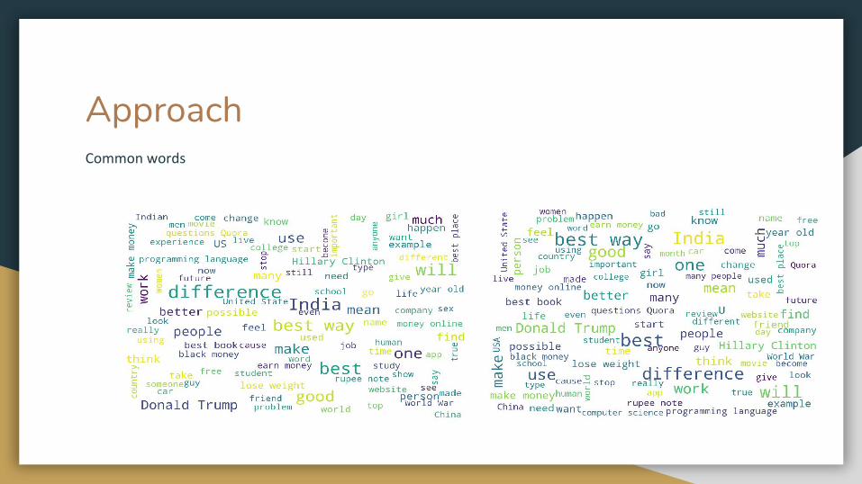
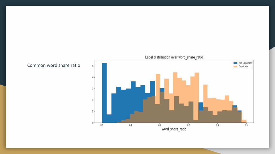
Approach

Supervised learning
●●●●●


Bag Of Words Model
● Convert the raw data into tf-idf features● Ngrams range - 1, 2, 3, 4● Minimum Document Frequency - 0, 10, 100, 200, 400, 600● Classifiers used - Logistic Regression, XGBoost

LSTM with Attention
● 2 layers of biLSTM● Attention layer● GLOVE word embedding● Optimizer - Adam● Loss function - Binary cross entropy

Results
●
●●

Results
●

Conclusion
●
●
●

Deep Clinic
By Ashok Govinda Gowda Saagar Minocha
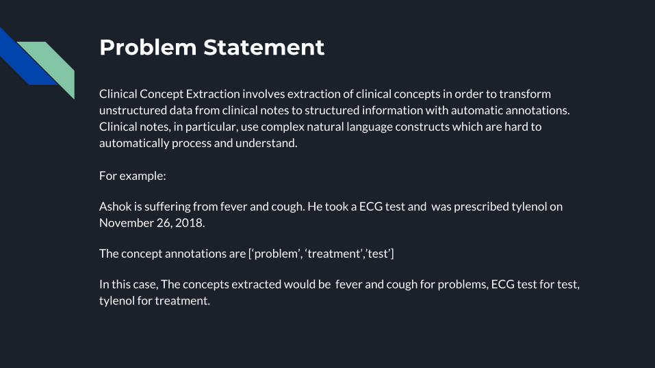
Problem Statement
Clinical Concept Extraction involves extraction of clinical concepts in order to transform
unstructured data from clinical notes to structured information with automatic annotations.
Clinical notes, in particular, use complex natural language constructs which are hard to
automatically process and understand.
For example:
Ashok is suffering from fever and cough. He took a ECG test and was prescribed tylenol on
November 26, 2018.
The concept annotations are [‘problem’, ‘treatment’,’test’]
In this case, The concepts extracted would be fever and cough for problems, ECG test for test,
tylenol for treatment.

Challenges
● Ambiguity of medical terms and concepts,● Use of non-standard acronyms● Out of vocabulary words● Lack of good annotated corpus● Complexity of sentence structures
○ conditional constructs (denoting future events)○ negated constructs (denoting absence of concepts)○ uncertain constructs (denoting uncertain events)○ historical constructs (denoting patient’s history)○ familial constructs (denoting patient’s genetical history)

Proposed Solution Overview
● Data Preprocessing● BIO-Tagging● Baseline Approach (using CRF)● Parameter Tuning● Deep Learning Approach (using CNN-BiLSTM)● Experimenting with Word Embeddings

DataSetInformatics for Integrating Biology and the Bedside (i2b2) 2010 dataset
https://www.i2b2.org/NLP/DataSets/Main.php
i2b2 2010/VA Training Test
Summaries 170 256
Sentences 16,414 27,613
Problems (Annotated Entities) 7,073 12,592
Treatments (Annotated Entities) 4,844 9,344
Test (Annotated Entities) 4,608 9,225

Data Formats

BIO tagging
BIO tagging is a format for tagging tokens in a chunking task . The B- prefix before a tag
indicates that the tag is the beginning of a chunk, and an I- prefix before a tag indicates that the
tag is inside a chunk. The B- tag is used only when a tag is followed by a tag of the same type
without O tokens between them. An O tag indicates that a token belongs to no chunk.
For Example:
Ashok is suffering from fever cough
('Ashok, 'O'), ('is', 'O'), ('sufferning', 'O'), ('from', 'O'), ('fever', 'B-problem'), ('cough, 'I-problem'),

Conditional Random Fields Baseline Approach
As a Baseline Approach, Conditional Random fields was used.
Conditional Random fields are utilized in places where we have to take sequential information
into account. For example: In the previous sentence we had B-problem which would be followed
by any number of I-problems. We are taking this into account with Conditional Random fields.
For this we used the sklearn-crfsuite library to utilize conditional random fields.
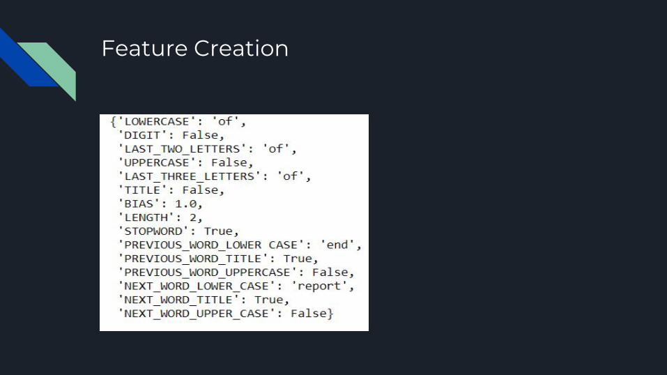
Feature Creation

Training Using L-BFGS Algorithm

Parameter Optimization Using Grid Search
Optimization of the parameters used in the Conditional Random fields was done using Grid
Search.
grid search, or a parameter sweep, which is an exhaustive searching through a manually
specified subset of the hyperparameter space of a learning algorithm. A grid search algorithm
must be guided by some performance metric, typically measured by cross-validation on the
training set or evaluation on a held-out validation set
Here the performance metric used while performing grid search was f1-score

Analysis of Relationships
Most Common Relationships
I-problem I-problem 3.066507
I-treatment I-treatment 2.978982
I-test I-test 2.786419
B-problem I-problem 2.51442
B-test I-test 2.41495
Least Common Relationships
O I-problem -7.86171
O I-test -7.526132
O I-treatment -7.295169
B-treatment I-problem -5.269959
B-treatment I-test -4.928459

Analysis of Word Features
The Most Common Word Features were
LOWERCASE:auscultation B-test
5.774259
LOWERCASE:hypertension B-problem
5.19519
LOWERCASE:apgars B-test 5.110699
LOWERCASE:srom B-problem 4.894952
LOWERCASE:fevers B-problem 4.871558
LOWERCASE:fever B-problem 4.869986
PREVIOUS_WORD_LOWER CASE:a
B-problem -3.738002
PREVIOUS_WORD_LOWER CASE:the
B-problem -3.506919
LOWERCASE:pain O -3.345862
LOWERCASE:sedated O -3.231368
PREVIOUS_WORD_LOWER CASE:# O
-3.131723
PREVIOUS_WORD_LOWER CASE:a B-test
-3.054437
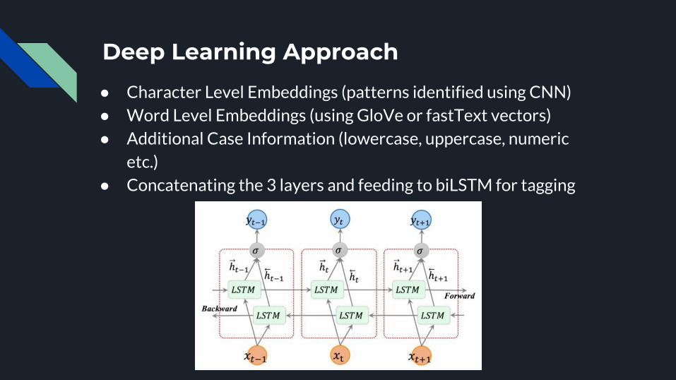
Deep Learning Approach
● Character Level Embeddings (patterns identified using CNN)● Word Level Embeddings (using GloVe or fastText vectors)● Additional Case Information (lowercase, uppercase, numeric
etc.)● Concatenating the 3 layers and feeding to biLSTM for tagging

Model Architecture

Word Embeddings● Stanford’s GloVe Vectors
glove.6B.50d - Wikipedia 2014 + Gigaword 5 (6B tokens, 400K vocab, uncased, 50d
vectors)
GloVe constructs a co-occurrence matrix (words X context) to count how frequently a
word appears in a context in order to learn. Factorization of this big matrix is usually done
to achieve a lower-dimension representation.
● Facebook’s fastText Vectorswiki-news-300d-1M.vec: 1 million word vectors trained on Wikipedia 2017, UMBC
webbase corpus and statmt.org news dataset (16B tokens).
fastText uses n-gram characters as the smallest unit to generate better word embeddings
(array of numbers with predefined dimensions) for rare words and out of vocabulary
words as the n-gram character vectors are shared with other words
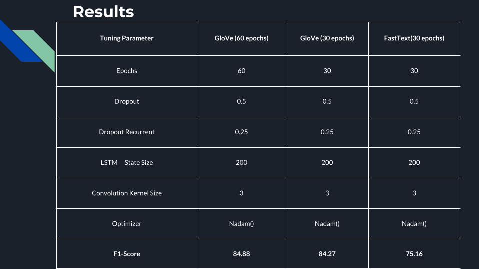
ResultsTuning Parameter GloVe (60 epochs) GloVe (30 epochs) FastText(30 epochs)
Epochs 60 30 30
Dropout 0.5 0.5 0.5
Dropout Recurrent 0.25 0.25 0.25
LSTM State Size 200 200 200
Convolution Kernel Size 3 3 3
Optimizer Nadam() Nadam() Nadam()
F1-Score 84.88 84.27 75.16

Conclusion
● Preprocessed raw data from an i2b2 dataset of clinical summaries
● Converting it to a BIO tagged format.● Established a statistical baseline using Conditional Random
Fields and achieved a fairly good F1-score of around 80%. ● Hyperparameter Tuning● Composed a neural network model using a bi-LSTM and a
character-level CNN achieving an F1-score of around 85% (higher than the baseline results)
● Experimented with fastText Embeddings

Thank You

Questions?

MOTIVATION
• Communication vs Language
• Piaget’s Four stages
1st: Sensorimotor Stage (birth ~ 2yrs)
1st & 2nd: Object permanence & Causality
• Combine Sensorimotor control with Language

BACKGROUND
[1] introduced neural process network.
• Could track common sense attributes through neural simulation of action dynamics.
• Data set: > 120, 000 recipes (JSON).
• No codes released yet.
References:
[1] Simulating Action Dynamics with Neural Process Networks, Antoine Bosselut, Omer Levy, Ari Holtzman, Corin Ennis, Dieter Fox, Yejin Choi, May,
2018, arXiv: 1711.05313.

EXAMPLE
Sausage beef ribs rigatoni (first 3 steps)
Text:
• In a large pan, sauté onions and garlic in oil until tender;
• Remove and set aside;
• Add chuck to pan, brown on all sides, then remove to onion dish;
Action:
• sauté; remove; brown, add, remove.
Ingredients:
• olive oil, onion, cloves garlic; same as previous; onion, chuck cut.

ORIGINAL ARCHITECTUREWORD2VECTOR

TRAINING AND RESULTS
• Each stage train independently
• No information about how accurate the system could achieve except for entity
selector with F1 score (vague) ~55%.
F1 score defined as:
2 ×𝑃𝑟𝑒𝑐𝑖𝑠𝑖𝑜𝑛×𝑅𝑒𝑐𝑎𝑙𝑙
𝑃𝑟𝑒𝑐𝑖𝑠𝑖𝑜𝑛+𝑅𝑒𝑐𝑎𝑙𝑙where 𝑃𝑟𝑒𝑐𝑖𝑠𝑖𝑜𝑛 =
𝑇𝑃
𝑇𝑃+𝐹𝑃, 𝑅𝑒𝑐𝑎𝑙𝑙 =
𝑇𝑃
𝑇𝑃+𝐹𝑁
• My trail: ingredient/action selector accuracy: ((TP+FN))/total 0.5%~1%.

A GLANCE

OTHER PROBLEMS
Four Corpora (high dimensional spaces)
• First three, text (7355), ingredient (2994), action (384)
• Last one, states change (~380)

ARCHITECTURE UPGRADEDWORD2VECTOR
RN
N
Encodin
g w
ith GRU
MLPAction
Selector
MLP with action attention Entity
Selector
MLPState
Predictor
Fig 2
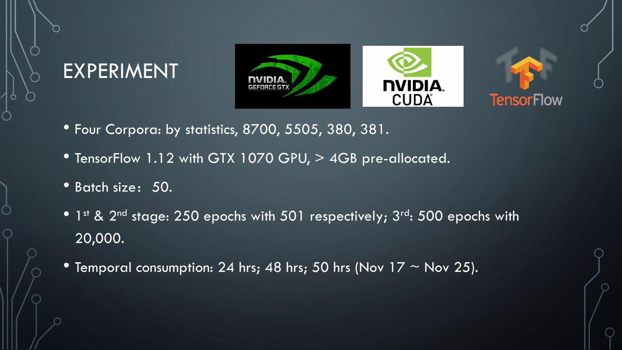
EXPERIMENT
• Four Corpora: by statistics, 8700, 5505, 380, 381.
• TensorFlow 1.12 with GTX 1070 GPU, > 4GB pre-allocated.
• Batch size:50.
• 1st & 2nd stage: 250 epochs with 501 respectively; 3rd: 500 epochs with
20,000.
• Temporal consumption: 24 hrs; 48 hrs; 50 hrs (Nov 17 ~ Nov 25).

RESULTS
• Accuracies for Entity/Action selectors (incredible): 5 starts.
• Accuracy for States change (good): 4 stars.
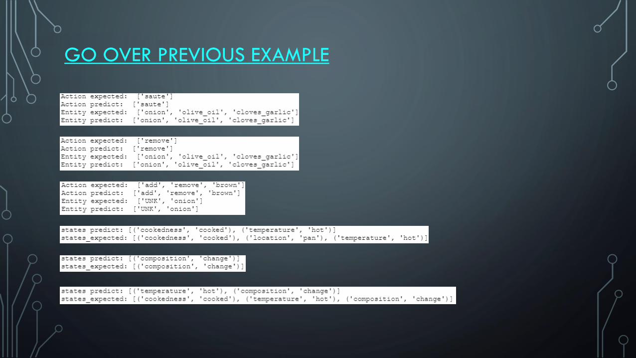
GO OVER PREVIOUS EXAMPLE

THANK YOU!

Q&A for US Pharma Industry
by APOORV KUMAR
Index
u Introduction
u Techniques adopted
u Results and discussion
u Conclusion

Introduction
u Currently, in the US Pharma industry, most of the product companies have the most important promotion channel as ‘physician calls’, which are delivered by sales reps
u Now, these sales reps usually want to access certain information about the doctor they will be meeting OR their own performance in their region.
u ~30-40% of sales rep don’t use the existing systems and rely on their previous understanding and hunch.

Index
u Introduction
u Techniques adopted
u Results and discussion
u Conclusion

Techniques adopted
u Method 1: Stanford SEMPRE Library –
u Stanford NLP group has created a Library called Sempre for the specific task of answering questions.
u Method 2: Using pre-defined question formats –
u Define question formats and then match the incoming requests to one of those questions

Method 1: Sempre library
u Sempre library was adopted because –
u All encompassing: By its design, it looks like one can answer a wide range of questions using a single process
u Scalable: Since Sempre uses a graph database called Virtuoso and a graph querying language calling SPARQL, it should be able to instantly produce answers even with large amount of data.
u Less production time as range of questions grow

Disadvantages of Sempre
u Not for complex questions: It is not specifically built for answering questions from tabular data, such as the one in this project.
u Lambda DCS is not a full-fledged programming language: The authors of this library themselves mention that the intent is not to create a complete programming language.
u One cannot select multiple columns of data. (Ex. in the question 'show address of doctors in zip 77840’, we will expect to see both names and address of doctors, but the current set of tools can only show one thing at a time (address or names)).
u Lack of appropriate documentation: Documentation is limited and there have been instances where some functionality was found but was not documented.
Method 2: Pre-defined question formats
u In this, several question formats are coded and then an incoming request is matched to one of those questions.
u On the implementation side, a question is converted to a set of filters, groupby columns and the columns to be selected.
u These parameters are sent to the server running in Flask in Python.
u MongoDB database is used since it provides the flexibility to incorporate the varied data in the project.
Index
u Introduction
u Techniques adopted
u Results and discussion
u Conclusion

Results and discussion
u Method 1: A sample of results from automated testing are as desired –
u The time is in ‘ms’

Index
u Introduction
u Techniques adopted
u Results and discussion
u Conclusion

Conclusion
u Sempre toolkit looks promising but it needs more functionality to make it useful for a question-answering project from tabular data
u The pre-defined question format method looks naïve but will be able to produce results faster in the beginning. This method will become challenging as the number of questions will grow.

Question Answering with the SQuAD dataset
CSCE 638 Final Project
Question Answering with the SQuAD dataset• Introduction
• Infersent model
• Passage (sentence) retrieval
• Qusestion Processing
• Answer Processing
• Answer Catching
• Accuracy
• Future Work
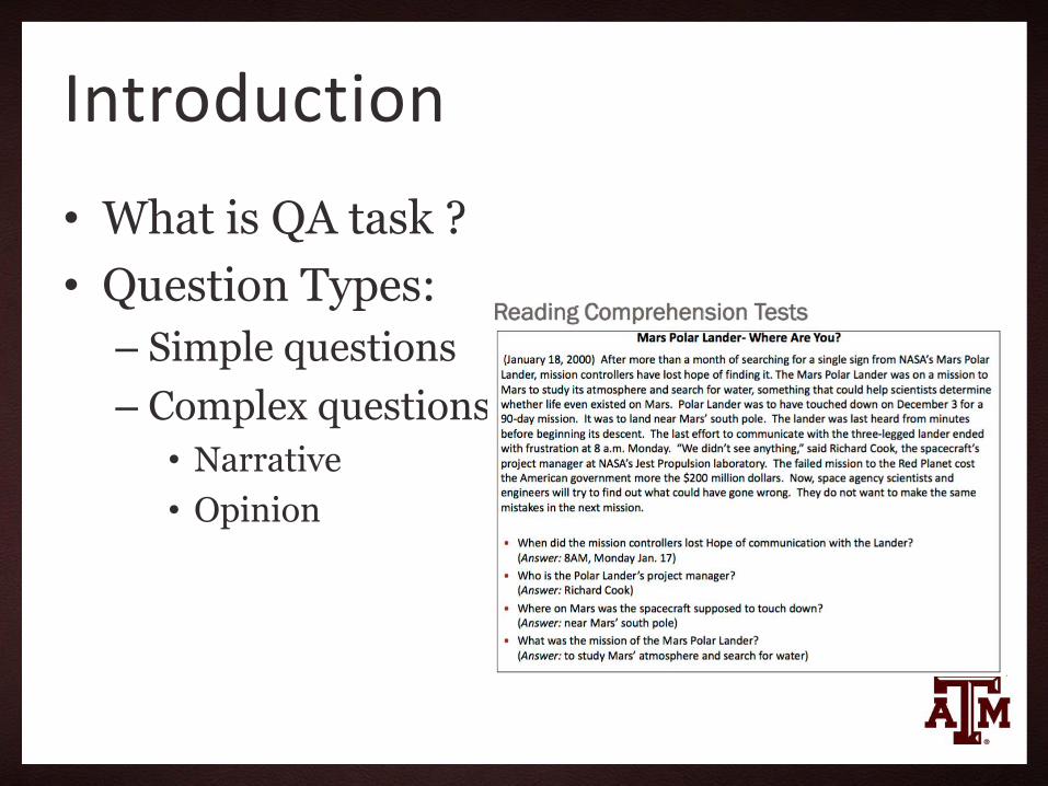
Introduction
• What is QA task ?
• Question Types:
– Simple questions
– Complex questions
• Narrative
• Opinion

Approaches
Qustions
Passage
(sentence)
Retrieval
Qusestion
Processing
Answer
Processing

Infersent model
• InferSent is a sentence embeddings method that provides semantic representations for English sentences
• How is Infersent implemented
• Model selection : trained on
GloVe dataset (discussed later)
Generic NLI training scheme.

Passage (sentence) retrieval on given context
• Split context by TextBlob
• Use Infersent for sentence embedding
• Evaluate similarity by distance like:
– Cosine similarity
– Euclidean Distance
– Manhattan Distance
– …

Passage (sentence) retrieval on given context
• Result:
Distance Metric Accuracy
Cosine similarity 0.6149162861491628
Euclidean distance 0.3995433789954338
Manhattan distance 0.43262481689453125
Chebyshev distance 0.2815829528158295
Accuracy of unsupervised learning base on
different distance

Passage (sentence) retrieval without context
• Get the context from Wikipedia page
• The other part is same as previous one
• Result:
– Question form SQuAD dataset: unsatisfying
– Custom Question: depends largely on the structure of question

Find Passage (sentence) retrieval without context
• Examples of questions from SQuAD dataset
Question 1 The Basilica of the Sacred
heart at Notre Dame is
beside to which structure?
Answer 1 The Basilica of the Sacred
Heart in Notre Dame, Indiana,
USA, is a Roman Catholic
church on the campus of the
University of Notre Dame, also
serving as the mother church
of the Congregation of Holy
Cross (C.S.C.)
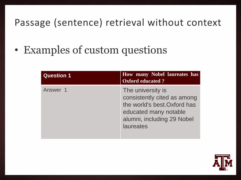
Passage (sentence) retrieval without context
• Examples of custom questions
Question 1 How many Nobel laureates has
Oxford educated ?
Answer 1 The university is
consistently cited as among
the world's best.Oxford has
educated many notable
alumni, including 29 Nobel
laureates

Model Selection : GloVe or fastText?
• Infersent V1 trained with GloVe
• Infersent V2 trained with fastText
• fastText shows poor performance
Distance Metric Accuracy
Cosine similarity 0.24885844748858446
Euclidean distance 0.2929984779299848
Manhattan distance 0.3036529680365297
Chebyshev distance 0.24733637747336376
Accuracy of unsupervised learning base on
different distance with Infersent trained on
fastText

Model Selection : GloVe or fastText?
• Why such difference?
• GloVe treats each word as an atomic entity and generated the corresponding vector.
• fastText treats each word as composed of character n grams
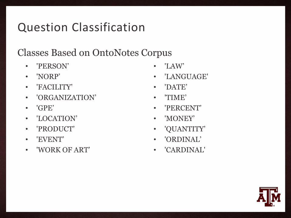
Question Classification
• 'PERSON’
• 'NORP’
• 'FACILITY’
• 'ORGANIZATION’
• 'GPE’
• 'LOCATION’
• 'PRODUCT’
• 'EVENT’
• 'WORK OF ART’
• 'LAW’
• 'LANGUAGE'
• 'DATE’
• 'TIME’
• 'PERCENT’
• 'MONEY’
• 'QUANTITY’
• 'ORDINAL’
• 'CARDINAL'
Classes Based on OntoNotes Corpus

Question Classification
Rules we used:
• Queries starting with “Who” or “Whom” are taken to be of type “PERSON”;
• Queries starting with “Where”, “Whence”, or “Whither” are taken to be of type “LOCATION”;
• Queries starting with “How few”, “How great”, “How little”, “How many” or “How much” are taken to be of type “QUANTITY”;
• Queries string with “Which” or “What”, look up head noun in lexicon to determine answer type.
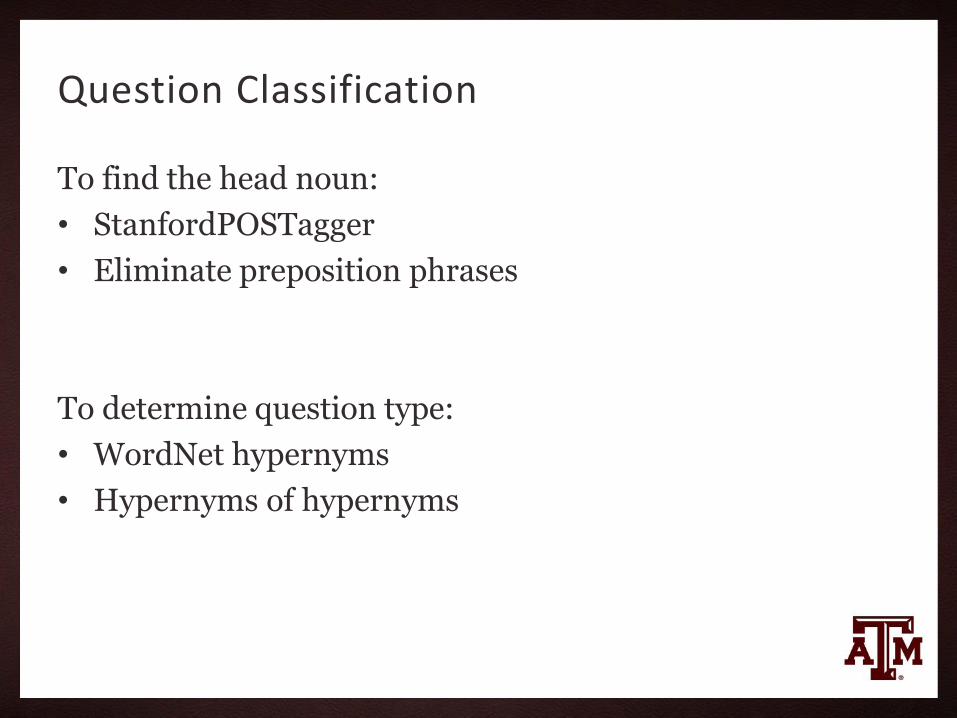
Question Classification
To find the head noun:
• StanfordPOSTagger
• Eliminate preposition phrases
To determine question type:
• WordNet hypernyms
• Hypernyms of hypernyms

Question Classification
# Determined with
Rule 1, 2, 3
# Determined with
Rule 4Others
379 618 317
Classification result:
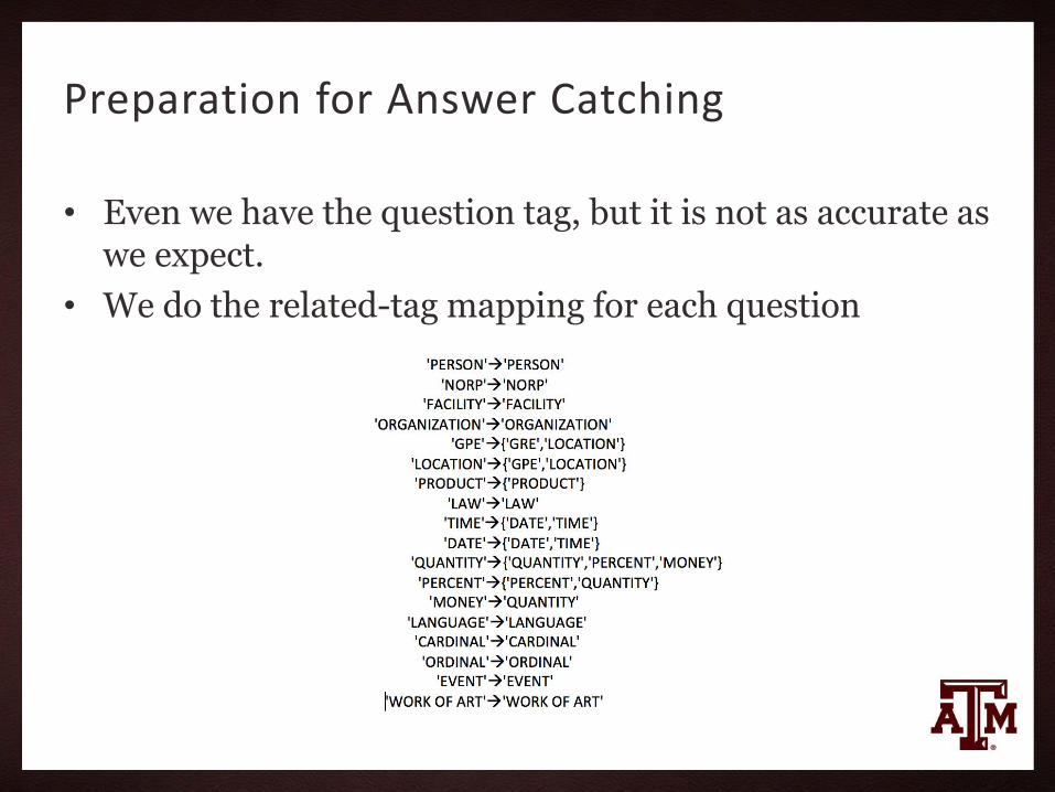
Preparation for Answer Catching
• Even we have the question tag, but it is not as accurate as we expect.
• We do the related-tag mapping for each question

Answer Catching
• tagged each word in target sentence using CogComp-NLP --CogComp-NLP provides a suite of state-of-the-art Natural Language
Processing (NLP) tools that allows you to annotate plain text inputs.
• Save word which hold same tag with question into answer list

Accuracy
• Full-Match Method
--all words in expected answer shown in result
• Partial-March Method
--at least one word in expected answer shown in result

Credits
Add your credits here
Machine Reading ComprehensionStuti Sakhi∗, Yerania Hernandez†
Department of Computer Science and EngineeringTexas A & M University∗Email: [email protected]
† Email: [email protected]
Abstract—Machine Reading Comprehension (MRC) allows theopportunity for a system to understand a given context andprovide an answer based on query on this context. In thispaper, we explore a variety of methods that have been developedto provide high F1 and exact match scorings on the SQuADdata set with the goal of implementing a multi-layer modelthat combines a variety of these features. We provide flexibilityin configuring a number of parmeters in order to analyze thedifferent configurations of networks. Our evaluation and resultsdemonstrate that our best model is a combination of GLoVeembeddings, an LSTM approach to RNN, a BiDAF weightattention, and a smart span method to provide the best answerpossible.
I. INTRODUCTION
Machine Reading Comprehension (MRC) provides the abil-ity for computers to read and understand natural language textand it can be considered as one of the necessary abilitiesfor artificial intelligence [1]. In order to train a system inanswering a query about a given paragraph, the model willneed to be able to create complex interactions and connectionsbetween the context provided and the query. Being able toextract such information definitely has its caveats, but couldbe beneficial for a number of domains, including improvingsearch engines in documents that are domain-specific andproviding support when answering customer service inquiries.Systems from previous works have achieved promising results,but are typically characterized by using attention weights onsummarized context, the attention weights are computed anddependent on previous steps, and attention layers are computedunidirectional, usually from query to context.
In this paper, we focus on exploring and analyzing a varietyof networks in order to find the best model to provide anadequate answer to the query given. The generic idea of ournetwork is to provide an embedding layer, an encoder layer,an attention layer, and the final output layer. Each of theselayers has a variety of features that were evaluated, includingcomparing word and character embeddings, the addition ofhighway layers, comparing Gated Recurrent Units (GRU) andLong Short Term Memory (LSTM) performance, using aunidirectional attention layer versus a Bi-Directional AttentionFlow (BiDAF) layer, and finally using softmax to predict thespan based on maximizing the probability distribution. Each ofthese features has demonstrated promising results individuallyand therefore, we combine a number of these features inorder to develop the best model to solve the MRC challenge.Our final model is able to outperform a number of previous
approaches from the SQuAD test set leader board. The rest ofthe paper is dedicated to describing a few previous approaches,further details on the data set we used and the approach wetook for each layer, the evaluation metrics we used, and thefinal results for the number of models we used along withfuture work for this task.
II. RELATED WORK
In order to tackle the MRC challenge, a major contributorto developing these models has been the number of largedatasets that have been developed and made available. In 2013,MCTest was too small of a dataset in order to be able totrain an end-to-end model [8]. In the recent years, industryhas provided additional attention to artificial intelligence andas result machine comprehension has become a strong factorin understanding natural text, which lead to CNN/DailyMaildataset in 2015 [5]. However, by 2016, the Stanford QuestionAnswering Dataset (SQuAD) was published providing anextensive dataset with a large number of questions, answers,and a wide-ranging of topics [6].
Typical end-to-end architectures have used a variety ofattention mechanisms, one of which depends on the previousstep for attention weights. Bahdanau et al. uses this approachreferred to as dynamically updating the weights [3]. However,Hermann et al. and Chen et al. demonstrate that the accuracyof the model can increase if a bilinear term is used in orderto compute the weights [5]. Furthermore, Kadlec et al. feedsthe attention weights after only computing them once intothe output layer without depending on previous weights [7].Each of these approaches are only unidirectional, where theanswer is derived from the correlation between the query tocontext and consider the answer is a single token, which isnot appropriate for the SQuAD data set. The BiDAF researchpaper describes the ability of performing an attention layerfrom context to question and question to context, whichdemonstrates a better performance than the previous uni-directional approaches [9]. In addition, Wang & Jiang exploredan LSTM architecture for natural language inference (NLI)and demonstrated how the network provides emphasis onword-level matches and relationships between words [12].Inspired from LSTM networks, highway layers have provento overcome the difficulty of training a network the deeperit increases considering deepness is crucial to a network’ssuccess [10]. Based on these features that have demonstratedimprovements to current machine comprehension tasks, we
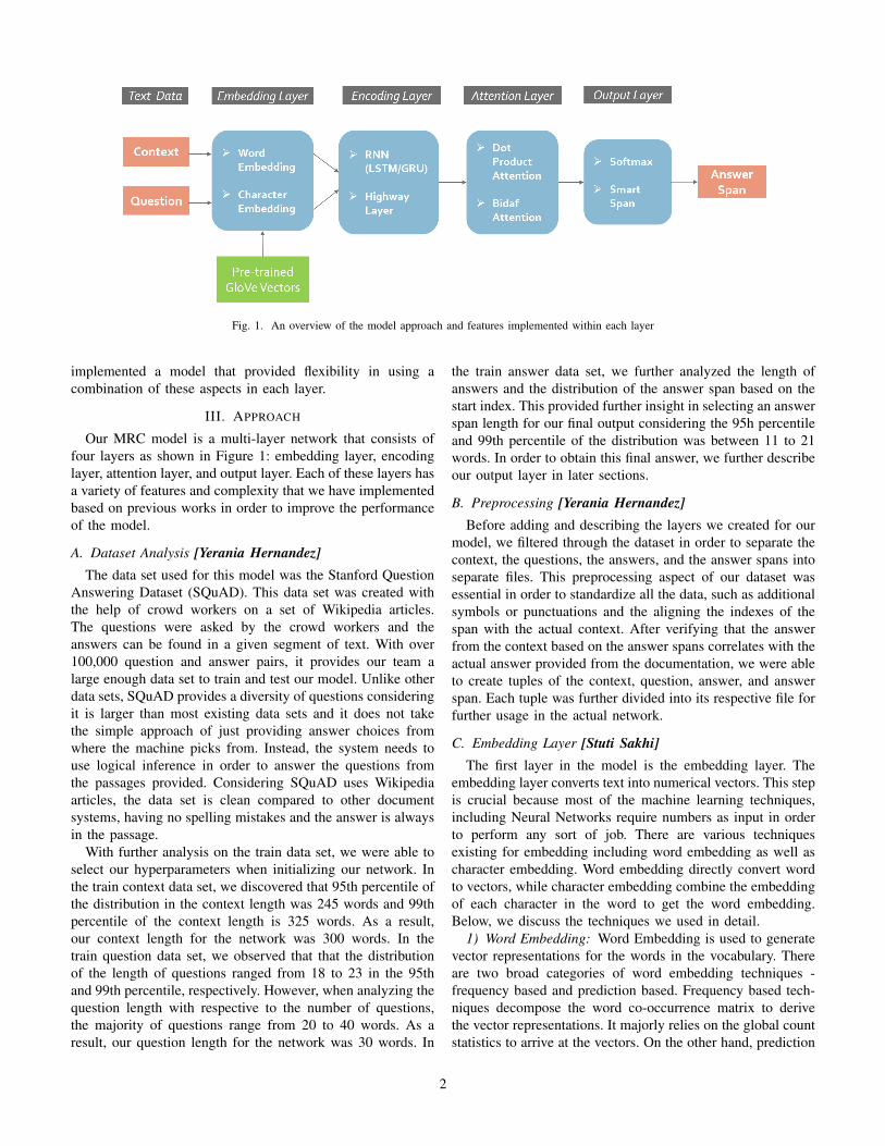
Fig. 1. An overview of the model approach and features implemented within each layer
implemented a model that provided flexibility in using acombination of these aspects in each layer.
III. APPROACH
Our MRC model is a multi-layer network that consists offour layers as shown in Figure 1: embedding layer, encodinglayer, attention layer, and output layer. Each of these layers hasa variety of features and complexity that we have implementedbased on previous works in order to improve the performanceof the model.
A. Dataset Analysis [Yerania Hernandez]The data set used for this model was the Stanford Question
Answering Dataset (SQuAD). This data set was created withthe help of crowd workers on a set of Wikipedia articles.The questions were asked by the crowd workers and theanswers can be found in a given segment of text. With over100,000 question and answer pairs, it provides our team alarge enough data set to train and test our model. Unlike otherdata sets, SQuAD provides a diversity of questions consideringit is larger than most existing data sets and it does not takethe simple approach of just providing answer choices fromwhere the machine picks from. Instead, the system needs touse logical inference in order to answer the questions fromthe passages provided. Considering SQuAD uses Wikipediaarticles, the data set is clean compared to other documentsystems, having no spelling mistakes and the answer is alwaysin the passage.
With further analysis on the train data set, we were able toselect our hyperparameters when initializing our network. Inthe train context data set, we discovered that 95th percentile ofthe distribution in the context length was 245 words and 99thpercentile of the context length is 325 words. As a result,our context length for the network was 300 words. In thetrain question data set, we observed that that the distributionof the length of questions ranged from 18 to 23 in the 95thand 99th percentile, respectively. However, when analyzing thequestion length with respective to the number of questions,the majority of questions range from 20 to 40 words. As aresult, our question length for the network was 30 words. In
the train answer data set, we further analyzed the length ofanswers and the distribution of the answer span based on thestart index. This provided further insight in selecting an answerspan length for our final output considering the 95h percentileand 99th percentile of the distribution was between 11 to 21words. In order to obtain this final answer, we further describeour output layer in later sections.
B. Preprocessing [Yerania Hernandez]Before adding and describing the layers we created for our
model, we filtered through the dataset in order to separate thecontext, the questions, the answers, and the answer spans intoseparate files. This preprocessing aspect of our dataset wasessential in order to standardize all the data, such as additionalsymbols or punctuations and the aligning the indexes of thespan with the actual context. After verifying that the answerfrom the context based on the answer spans correlates with theactual answer provided from the documentation, we were ableto create tuples of the context, question, answer, and answerspan. Each tuple was further divided into its respective file forfurther usage in the actual network.
C. Embedding Layer [Stuti Sakhi]The first layer in the model is the embedding layer. The
embedding layer converts text into numerical vectors. This stepis crucial because most of the machine learning techniques,including Neural Networks require numbers as input in orderto perform any sort of job. There are various techniquesexisting for embedding including word embedding as well ascharacter embedding. Word embedding directly convert wordto vectors, while character embedding combine the embeddingof each character in the word to get the word embedding.Below, we discuss the techniques we used in detail.
1) Word Embedding: Word Embedding is used to generatevector representations for the words in the vocabulary. Thereare two broad categories of word embedding techniques -frequency based and prediction based. Frequency based tech-niques decompose the word co-occurrence matrix to derivethe vector representations. It majorly relies on the global countstatistics to arrive at the vectors. On the other hand, prediction
2

based techniques take only local context into account and learnword embedding which capture meaning in the vector space.Considering the global count statistics and learning dimensionsof meaning both are equally crucial in deriving word embed-ding. Keeping this in mind, we went ahead with using GLoVeVectors for the word embedding as it combines the best of bothworlds. The GloVe vectors are learned by optimising a losswhich uses global count statistics information. We used thepre-trained GloVe vectors of dimension 100 for our project. Soeach word in the dataset(context and question) was convertedto a vector using these pre-trained GLoVe vectors.
2) Character Embedding: Character embedding is anotherway to convert text to vectors. Here we have a vector foreach character in our dataset. To get the word embedding wecombine the character embedding of the constituent characters.Character embeddings have less dimension as the numberof characters are limited. Moreover, character embeddingshelp us to utilise the internal structure of the word and alsohandle out of vocabulary words. We used the character levelConvolutional Neural Network(CNN) [9] to learn the characterembeddings.
For the character level CNN, we start with representing eachcharacter with trainable character embeddings c1, c2, ..,cl. Noweach word can be represented as e1, e2,.., ek using it. Now,these word representations are input into a 1 dimensional CNNto get the hidden state embedding of the words.The idea is that,each hidden vector is a combination of a window of charactersdue to the convolution. Both the embedding and filter for theCNN are learned during the training of this model.
D. Encoding Layer [Stuti Sakhi]Once we had the vector representation of words, our next
step was to make each word aware of the words before it andafter it. This is a very important step as words individuallyonly give partial information. It is the sentence which actuallyholds the complete meaning. To make each word aware of itscontext, we used a bidirectional Recurrent Neural Network.We also used the highway layer as a part of the encodingin some of the cases to model higher complexity. Now, wediscuss each of these in detail
1) Recurrent Neural Network: A recurrent neural net-work(RNN) which is capable of handling sequential data. Thehidden state in the RNN, remembers the previous instances andhence can handle sequential data. Figure 2 shows an unrolledRNN. Here, we can view inputs, X1, X2,.., Xn as the wordembedding of a sentence (context and answer in or case).Each of the hidden state Ht is found using the present inputXt and previous hidden state Ht-1. Equation 1 below showsthis relation. Whh and Wxh are learned during the training.
Ht = tanh(WhhHt−1 +WxhXt) (1)
RNN, in theory can remember information which wasprocessed long back. In reality however, they face an issueof diminishing gradient which does not allow them to do so.For this reason we decided to work with two modifications ofRNN, Long Short Term Memory(LSTM) and Gated Recurrent
Fig. 2. Recurrent Neural Network
Unit(GRU). Both of these add extra gates to the RNN, thusmaking it easier for information from past to pass.
A GRU uses an update gate and a reset gate. The updategate decides on how much of information from the past shouldbe let through and the reset gate decides on how much ofinformation from the past should be discarded. On the otherhand, LSTM has three gates forget gate, update gate andoutput gate. Hidden state is computed using the forget gateand update gate. The output gate determines how much muchrepresentation the hidden state must have in the output. LSTMand GRU are complex models when compared to a vanillaRNN. However, the added computation allows us to captureinformation from long sequences. Generally LSTM capturesmore information from past when compared to GRU. Wecompared the performance of both of these to find a betterfit for out data set.
To make sure words are aware of other words both fromleft as well as right, we used a bidirectional LSTM/GRU.Bidirectional LSTM/GRU just concatenate the the hiddenstates of two LSTM/GRU in opposite directions.
2) Highway Layer: Since this is a complex problem, wedecided to add more non linearity to the model by addingfully connected layers. However, as our model was alreadydeep, a fully connected layer would not perform well and wemight end up losing valuable information from the startinglayers. For this reason we decided to add in a highway layer[4]. A highway layer is inspired by LSTM. It has 2 gatestransform gate and the carry gate. The transform gate decideshow much of the input must be represented by the non lineartransformation while the carry gate decides how much of theinput must be passed as it is to the next layer. Lets supposex is the input to the highway layer, then the output y can bewritten as shown in equation (2). Here, H(tranformed input)is a function of Wh, T(tranform gate) is a function of Wt andC(carry gate) is a function of Wx. All the three Wh, Wt andWx are learned during the training.
y = H(x,Wh).T (x,Wt) + x.C(x,Wx) (2)
We tried out various combination in this layer GRU andLSTM with and without the highway layer.By the end of thislayer, we have the hidden state vectors for both context andthe question.
E. Attention Layer [Stuti Sakhi]Now that we have both the context and question hidden
layers, our next step would be to understand which part of thecontext is relevant to the question. This layer is called attentionas it decides where in the context we need to give attention in
3
order to answer the given question. Intuitively speaking, thislayer will output a vector which assigns weights to each wordin the context according to their relevance with the question.We tried out two attention mechanisms, Dot Product Attentionand Bidirectional Attention flow in our implementation.Wediscuss the two in detail below.
1) Dot Product Attention: Dot Product Attention is one ofthe most primitive attention mechanisms. Lets denote questionencodings as q1,q2,..,qM and context encodings as c1, c2,...cN.We evaluate the attention distribution i for each context stateci as follows.
ei = [cTi q1 cTi q2...c
Ti qM ] (3)
αi = softmax(ei) (4)
Now we take the weighted sum of the question hidden statesqi to get the attention output ai for each context state ci.
ai =
M∑j=1
αijqj (5)
Then finally we concatenate each of these ai to ci to get thefinal attention output hidden state bi
bi = [ci; ai] (6)
There is no learning involved in this Dot product attention.2) Bidirectional Attention Flow Mechanism: Bidirectional
Attention Flow is a high performing attention mechanism [9].It is based on the idea that attention must flow both ways, fromquestion to context as well as context to question. Lets denotequestion encodings as q1,q2,..,qM and context encodings as c1,c2,...cN. We evaluate each element Sij of the similarity matrixS such that
Sij =WTs [ci; qj ; ci · qj ] (7)
Here Ws is learned during the training. Now, first we performContext to Question attention. For each context hidden stateci we evaluate ai according to the following equations.
αi = softmax(Si:) (8)
ai =
M∑j=1
αijqj (9)
Now, for the Question to Context, firstly for each i from 1 toN we find mi. All the mi are concatenated to get m.Then c’,the question to context coefficient is evaluated.
mi = maxj(Sij) (10)
β = max(m) (11)
c′ =
N∑i=1
βici (12)
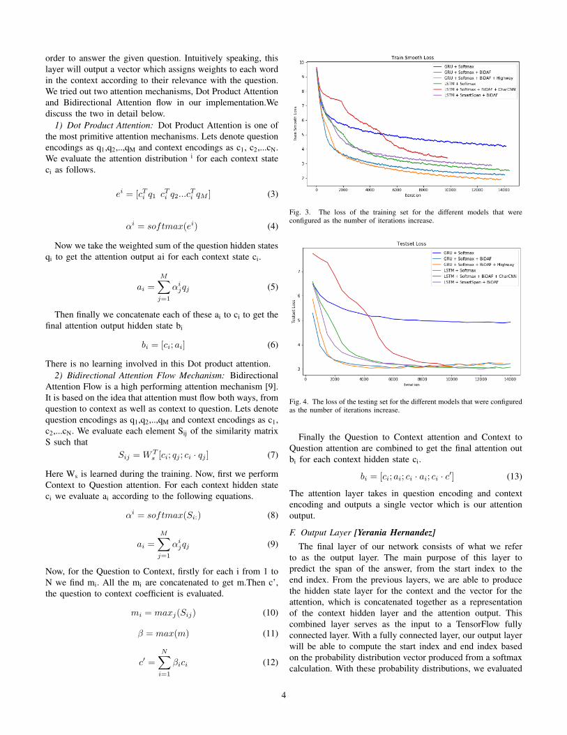
Fig. 3. The loss of the training set for the different models that wereconfigured as the number of iterations increase.
Fig. 4. The loss of the testing set for the different models that were configuredas the number of iterations increase.
Finally the Question to Context attention and Context toQuestion attention are combined to get the final attention outbi for each context hidden state ci.
bi = [ci; ai; ci · ai; ci · c′] (13)
The attention layer takes in question encoding and contextencoding and outputs a single vector which is our attentionoutput.
F. Output Layer [Yerania Hernandez]The final layer of our network consists of what we refer
to as the output layer. The main purpose of this layer topredict the span of the answer, from the start index to theend index. From the previous layers, we are able to producethe hidden state layer for the context and the vector for theattention, which is concatenated together as a representationof the context hidden layer and the attention output. Thiscombined layer serves as the input to a TensorFlow fullyconnected layer. With a fully connected layer, our output layerwill be able to compute the start index and end index basedon the probability distribution vector produced from a softmaxcalculation. With these probability distributions, we evaluated
4

TABLE IRESULTS FOR SQUAD TRAIN AND TEST SET
Embedding Layer EncodingLayer
AttentionLayer
Output Layer Dropout F1 Score EM Score
Train Test Train Test
Glove GRU Dot Product Softmax 0.85 57.41 36.47 45.30 25.95
Glove GRU BiDAF Softmax 0.85 85.01 64.28 72.70 49.11
Glove GRU +Highway
BiDAF Softmax 0.85 89.41 65.47 77.30 50.46
Glove LSTM BiDAF Softmax 0.75 81.29 64.83 66.70 50.18
Glove + Char CNN LSTM BiDAF Softmax 0.70 69.07 61.95 55.50 46.89
Glove LSTM BiDAF Smart Span 0.75 77.66 66.43 64.90 50.56
two different methods in order to obtain the final start andend indexes. The basic method obtains the maximum indexprobability from the start and end distribution vectors andreturns this as the start and end index. The second method,which we refer to as a smart span method, is based on theanalysis we had done on our data set. Considering we knowthat answers span between 11 to 21 words, we selected 15 asthe maximum words that the answer should span. As a result,we are able to maximize the probability through the product ofthe start and end distribution vector in order to obtain the beststart and end index. After all these layers have been initialized,we add a loss layer, which simply computes the cross-entropyloss for the start and end index predictions while also usingthe Adam optimizer in order to minimize the loss across eachbatch.
IV. EVALUATION [STUTI SAKHI]We use two evaluation criteria to evaluate our model.1) Exact Match (EM) : It is a binary measure which
checks if the predicted answer matches exactly the actualanswer.
2) F1 : F1 is a harmonic mean of precision and recall. Pre-cision the percentage of words in the predicted answerwhich are present in the actual answer. Recall is thepercentage of words from the actual answer which arepresent in the predicted answer.
V. RESULTS [YERANIA HERNANDEZ]Our entire network was developed with a variety of param-
eters in order to allow us the flexibility of testing differentconfigurations. These different networks were implementedusing Tensorflow 1.11 and Python 3.6, while training onGoogle Colab due to the available Tesla K80 GPU. The resultsof the different model configurations we experimented withare summarized in Table I. As shown, the model with thebest configuration uses GLoVe vectors, the LSTM networkin the encoding layer, BiDAF attention in the attention layer,and the smart span method in the output layer. The F1 scoreof this model on the test set is 66.43 and the EM score is
50.56, which performs comparable to the scores displayedon the leader board of the SQuAD data set. In addition,Figure 3 demonstrates the loss of the train set of each of theconfigurations as the number of iterations increases. The mostbasic configuration consists of using the GRU network witha softmax as part of the output layer. As the graph displays,the loss is much higher than any of the other configurations.Furthermore, this loss is also replicated in the test set, asshown in Figure 4. All the other configurations demonstratelow losses along with reaching this stage at a much quickerpace. Each of these configurations were run from ten epochs tofifteen epochs, causing them to run for over 14,000 iterations.However, after a certain number of iterations, it is visible thatthe loss converges.
In addition to the different features we explored within eachlayer, we also analyzed the effects of certain hyperparameters.After training a few configurations, we observed that accuracyscoring between the train and test had a difference of overtwenty points. This concerned us due to the fact that it couldbe possible that our network was overfitting the results. As aresult, we began decreasing the dropout ratio in order to reducethis difference between the training and test set. As is shown inTable I, the decrease in dropout reduced the difference betweenthe train and test set to about ten points. This differenceseemed more reasonable considering these results were morecorrelated to each other and therefore we used 0.75 as thedropout ratio for our final model. In addition, we analyzedthe decrease of the learning rate and the effects it had onthe scoring as well. However, we only had the opportunityto configure two different learning rates and although it didincrease the scoring of our configurations, we cannot make acomplete conclusion on the actual effect it had on our results.Our final model used a 0.0008 learning rate instead of theinitial 0.001 used for the base model considering previousworks focused on the importance of having a low learningrate.
5

VI. CONCLUSION
In this paper, we focused on exploring a variety of ap-proaches to develop an MRC model to analyze the SQuADdata set. Our results demonstrate that our best model usesa combination of GLoVe word embedding, LSTM network,BiDAF attention, and smart span to finalize the appropriateanswer based on the query and context provided. The analysison these different configurations provides an insight on thedifferent aspects that have been taken into account to solvethe MRC challenge. As a result, we obtained a model thatperformed similar to some of the methods published onthe SQuAD data set leader board. Future work consists ofexploring hyperparameters and other configurations, whichcould possibly increase the F1 and EM score. In addition,due to the flexibility we add to our model, we could furtherextend this model to implement other types of recurrent neuralnetworks.
REFERENCES
[1] “2018 NLP Challenge on Machine Reading Comprehension.”2018 NLP Challenge on Machine Reading Comprehension, 2018,mrc2018.cipsc.org.cn/.
[2] Dwivedi, and Priya Dwivedi. “NLP - Building a Question AnsweringModel – Towards Data Science.” Towards Data Science, Towards DataScience, 29 Mar. 2018, towardsdatascience.com/nlp-building-a-question-answering-model-ed0529a68c54.
[3] Dzmitry Bahdanau, Kyunghyun Cho, and Yoshua Bengio. Neural machinetranslation by jointly learning to align and translate. ICLR, 2015.
[4] Fleming, Jim. “Highway Networks with TensorFlow – Jim Fleming– Medium.” Medium.com, Medium, 29 Dec. 2015, medium.com/jim-fleming/highway-networks-with-tensorflow-1e6dfa667daa.
[5] Karl Moritz Hermann, Tomas Kocisk y, Edward Grefenstette, LasseEspeholt, Will Kay, Mustafa Suleyman, and Phil Blunsom. Teachingmachines to read and comprehend. In NIPS, 2015.
[6] Pranav Rajpurkar, Jian Zhang, Konstantin Lopyrev, and Percy Liang.Squad: 100,000+ questions for machine comprehension of text. InEMNLP, 2016.
[7] Rudolf Kadlec, Martin Schmid, Ondrej Bajgar, and Jan Kleindienst. Textunderstanding with the attention sum reader network. In ACL, 2016.
[8] Richardson, Matthew, et al. “MCTest: A Challenge Dataset for the Open-Domain Machine Comprehension of Text.” 2013 Conference on EmpiricalMethods in Natural Language Processing, 2013.
[9] Seo, Minjoon, et al. “BI-DIRECTIONAL ATTENTION FLOWFOR MACHINE COMPREHENSION.” ICLR 2017, 2017,doi:https://arxiv.org/pdf/1611.01603.pdf.
[10] Srivastava, Rupesh Kumar, et al. “Training Very Deep Networks.” 2015.[11] Wang, Shuohang, and Jing Jiang. “Learning Natural Language Inference
with LSTM.” Cornell University Lab, American Physical Society, 10 Nov.2016, arxiv.org/abs/1512.08849.
[12] Wang, Shuohang, and Jing Jiang. “MACHINE COMPREHENSIONUSING MATCH-LSTM AND ANSWER POINTER.” ICLR 2017, 2017,doi:https://arxiv.org/pdf/1608.07905.pdf.
6

Math Question AnsweringTao Ni
Kunping Huang
Yiran Huang

Syntactic Parsing
u According to the thesis:
u Backward application of an XTOP (extended top-down tree-to-string) transducer
u Supported by packages like Tiburon (May and Knight, 2006)
u About 140 states, and 550 engineered rules

Syntactic Parsing
u According to the thesis:

Syntactic Parsing
u Our implementation:
u The Tiburon package is not so easy to use
u Instead using nltk.parse.chart.BottomUpLeftCornerChartParser
u This parser can handle left recursions in rules
u About 50 states and 250 rules

Syntactic Parsing
u Sample results:
Q:
If \(a-5=0\), what is
the value of
\(a+5\)?
Syntactic Parsing
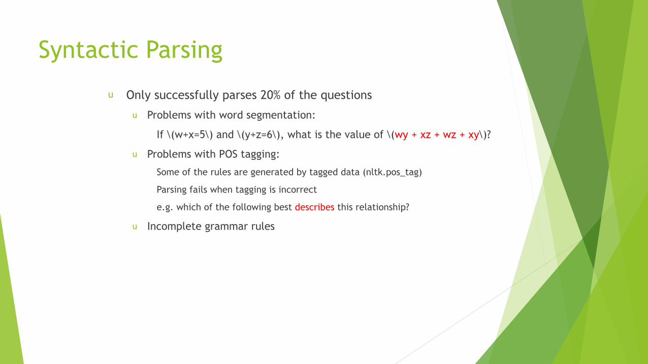
u Only successfully parses 20% of the questions
u Problems with word segmentation:
If \(w+x=5\) and \(y+z=6\), what is the value of \(wy + xz + wz + xy\)?
u Problems with POS tagging:
Some of the rules are generated by tagged data (nltk.pos_tag)
Parsing fails when tagging is incorrect
e.g. which of the following best describes this relationship?
u Incomplete grammar rules

Semantics Parsing
u Multi Bottom-up Tree Transducer
u Semantics Parsing
u Anaphora resolution
u Semantic translation

Multi Bottom up Tree Transducer
u Math Question: ⟨r, s, t⟩ In the sequence above, if each term after the first is x more than the previous term, what is the average of r, s, and t in terms of r and x?
u The term refers to the term in ⟨r, s, t⟩.
u The typical semantic parser does not work.

Multi Bottom up Tree Transducer
S
NP
N
people
VP
V NP PP
N P NP
N
fish tanks with rods
S
ActionAgent Tool
Subj Obj
fish people tanks rods

Initial State
S
NP
N
people
VP
V NP PP
N P NP
N
fish tanks with rods
S
1

Intermedia State
S
NP
N
people
VP
V NP PP
N P NP
N
fish tanks with rods
1
S
ActionAgent Tool
Subj Obj
1
1
2
3
S
NP VP
S
ActionAgent Tool
Subj Obj
1
12
3
Rule:

Intermedia State
S
NP
N
people
VP
V NP PP
N P NP
N
fish tanks with rods
1
1
2
3
Rule:NP
N
people
Subj
people
S
ActionAgent Tool
Subj Obj
people

Intermedia State
S
NP
N
people
VP
V NP PP
N P NP
N
fish tanks with rods
1
2
3
S
ActionAgent Tool
Subj Obj
people

VP
V NP PP
N P NP
N
fish tanks with rods
Action
fish
Obj
tanks
Tool
rods
Rule:

Multi Bottom up Tree Transducer
S
NP
N
people
VP
V NP PP
N P NP
N
fish tanks with rods
S
ActionAgent Tool
Subj Obj
fish people tanks rods

Tree to Tree Rules
EN
EN ENADD
ADD
ENEN
transitions
lhs rhs
Complex Aggregations
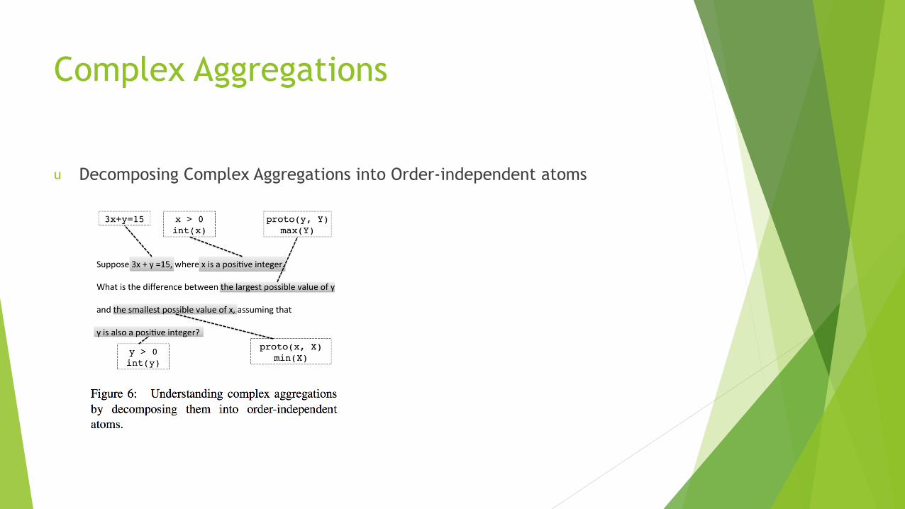
u Decomposing Complex Aggregations into Order-independent atoms

u Z3 solver:
u Z3 is a Satisfiability Modulo Theories (SMT) solver.
u Z3Py: the Z3 API in Python
x, y, z = Reals('x y z')
s = Solver()
s.add(x > 1, y > 1, x + y > 3, z - x < 10)
print s.check()
u Cannot handle output directly
Interpretation
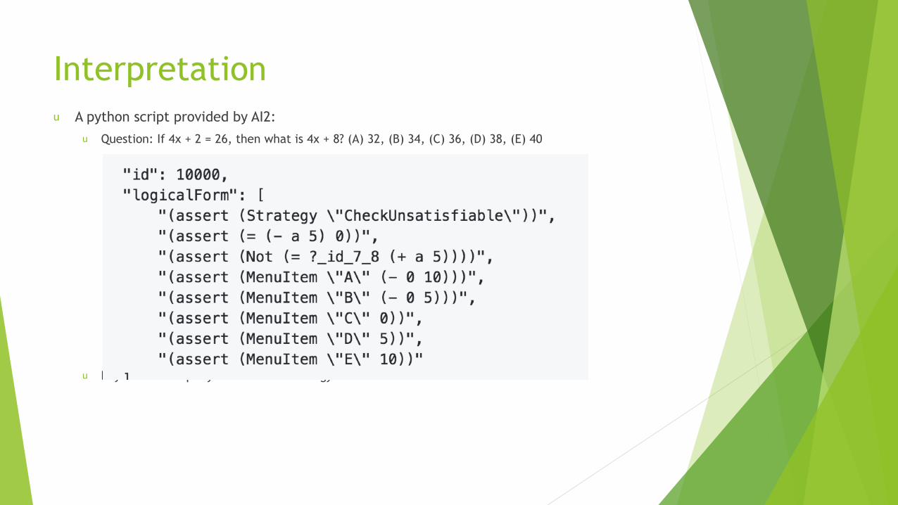
Interpretationu A python script provided by AI2:
u Question: If 4x + 2 = 26, then what is 4x + 8? (A) 32, (B) 34, (C) 36, (D) 38, (E) 40
u Key elements: query variable and strategy.

Result
u It is not easy to find the appropriate rules for semantic parsing. So far we haven't worked out a single logical form.
Conclusion
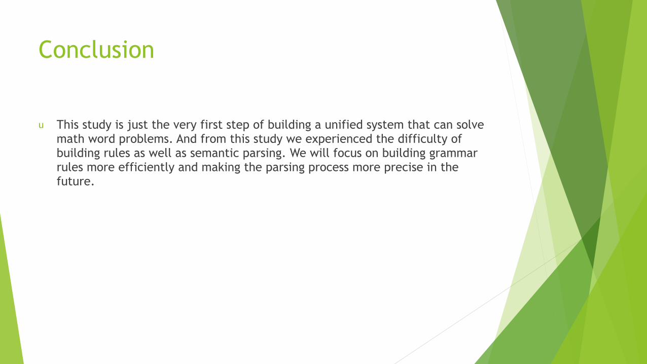
u This study is just the very first step of building a unified system that can solve math word problems. And from this study we experienced the difficulty of building rules as well as semantic parsing. We will focus on building grammar rules more efficiently and making the parsing process more precise in the future.

Q&A

Visual Question AnsweringZhengyang Wang, Yi Liu, Yaochen Xie
CSCE-638: NLP Foundation and Techniques
Dec 4, 2018
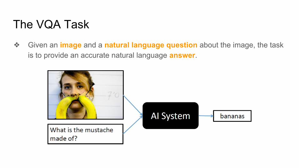
The VQA Task❖ Given an image and a natural language question about the image, the task
is to provide an accurate natural language answer.

Our Approach
Architecture Overview

Our Approach

Our Approach

Our Approach
Word Embedding: word2vec/GloVe/BERT
❖ Euclidean/cosine distance between two vectors measures the similarity of two words
❖ Linear substructures
man - woman city - zip code
comparative - superlative

Our Approach
Word Embedding: word2vec/GloVe/BERT
❖ Bi-directional Transformer (attention-based)❖ Contextual embedding

Our Approach

Our Approach
Convolution & (Multi-head) Self-attention
A weighted sum on Value
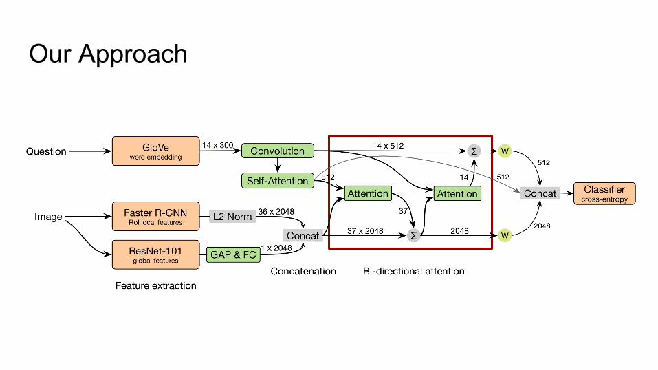
Our Approach

Our Approach
Question-to-image attention
And the Image-to-question attention works similarly.
Why do we use bi-directional attention?
A weighted sum onRoI (& global) features

Our Approach

Dataset & Evaluation❖ Dataset we used: VQA v2.0
❖ Evaluation➢ An evaluation metric that robust to inter-human variability in phrasing the
answers:
Images Questions Annotations
Training 82,783 443,757 4,437,570
Validation 40,504 214,354 2,143,540

Experimental ResultsEarly stopping at 120k-th iteration to avoid overfitting.
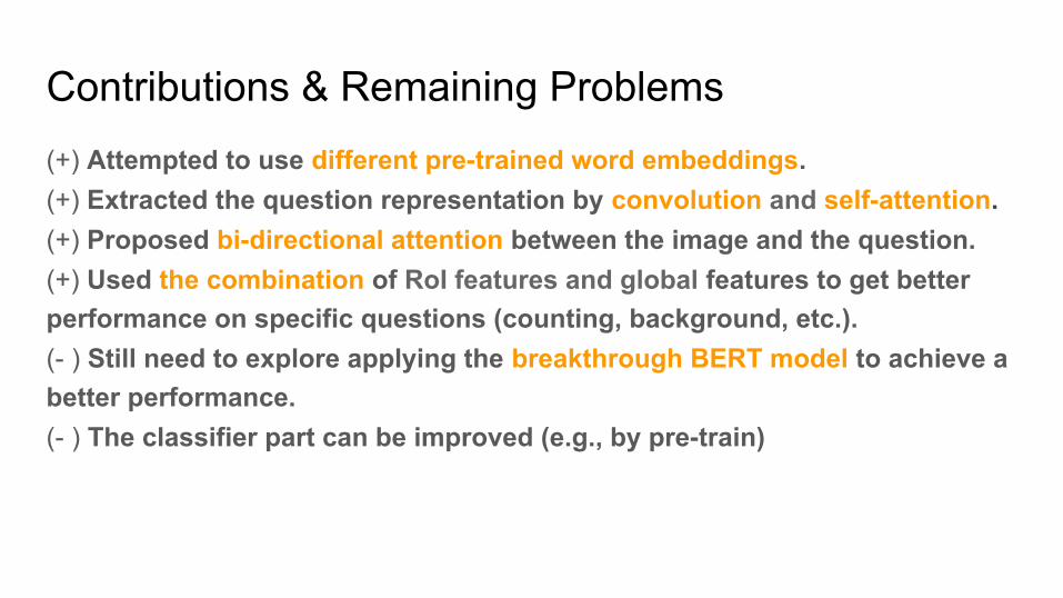
Contributions & Remaining Problems(+) Attempted to use different pre-trained word embeddings.(+) Extracted the question representation by convolution and self-attention.(+) Proposed bi-directional attention between the image and the question.(+) Used the combination of RoI features and global features to get better performance on specific questions (counting, background, etc.).(- ) Still need to explore applying the breakthrough BERT model to achieve a better performance.(- ) The classifier part can be improved (e.g., by pre-train)