1  

Simple and Robust Rules for Monetary Policy

by

John B. Taylor and John C. Williams

Preliminary Draft Prepared for the Handbook of Monetary Economics Edited by Benjamin Friedman and Michael Woodford

October 2009

Economists have been interested in monetary policy rules since the advent of economics.

In this review paper we concentrate on more recent developments, but we begin with a brief

historical summary to motivate the theme and purpose of our paper. We then describe the

development of the modern approach to policy rules and evaluate the approach using experiences

before, during, and after the Great Moderation. We then contrast in detail this policy rule

approach with optimal control methods and discretion. Finally we go on to consider several key

policy issues, including the zero bound on interest rates and issue of bursting bubbles, using the

lens of policy rules.

1. Historical Background

Adam Smith first delved into the subject monetary policy rules in the Wealth of Nations

arguing that “a well-regulated paper-money” could have significant advantages in improving

economic growth and stability compared to a pure commodity standard. By the start of the 19th

century Henry Thornton and then David Ricardo were stressing the importance of rule-guided

monetary policy after they saw the monetary-induced financial crises related to the Napoleonic Wars.

Early in the 20th century Irving Fisher and Knut Wicksell were again proposing monetary policy

rules to avoid monetary excesses of the kinds that led to hyperinflation following World War I or

2  

seemed to be causing the Great Depression. And later, after studying the severe monetary

mistakes of the Great Depression, Milton Friedman proposed his constant growth rate rule with

the aim of avoiding a repeat of those mistakes. Finally, modern-day policy rules, such as the

Taylor Rule, were aimed at ending the severe price and output instability during the Great

Inflation of the late 1960s and 1970s. (See Asso, Kahn, and Leeson (2007) for a detailed

review).

As the history of economic thought makes clear, a common purpose of these reform

proposals was a simple stable monetary policy that would both avoid monetary shocks and

cushion the economy from other shocks, and thereby reduce the chances of recession,

depression, crisis, deflation, inflation, or hyperinflation. There was a presumption in this work

that some such simple rule could improve policy by avoiding monetary excesses, whether related

to money finance of deficits, commodity discoveries, gold outflows, or mistakes by central

bankers with too many objectives. The choice between a monetary standard where the money

supply jumped around randomly versus a simple policy rule with a smoothly growing money and

credit seemed like a no brainer. The choice was both broader and simpler than “rules versus

discretion.” It was “rules versus chaotic monetary policy” whether the chaos was caused by

discretion or simply exogenous shocks like gold discoveries or shortages.

A significant change in economists’ search for simple monetary policy rules occurred in

the 1970s, however, as a new type of macroeconomic model appeared on the scene. The new

models were dynamic, stochastic, and empirically estimated. And because they incorporated both

rational expectations and sticky prices, they were sophisticated enough to serve as a laboratory to

examine how monetary policy rules would work in practice. These were the models that were

used to find new policy rules, such as the Taylor Rule, to compare the new rules with earlier

3  

constant growth rate rules or with actual policy, and to check the rules for robustness. Examples

include the simple three equation model in Taylor (1979), the multi-equation international

models in the comparative studies by Bryant, Hooper, and Mann (1993), and the econometric

models in robustness analyses of Levin, Wieland, and Williams (1999). More or less

simultaneously practical experience was confirming the model simulation results as the

instability of the Great Inflation of the 1970s gave way to the Great Moderation around the same

time that actual monetary policy began to resemble the simple policy rules that were proposed.

While the new rational expectations models with sticky prices further supported the use

of policy rules (because of the Lucas critique and time inconsistency), there was no fundamental

reason why the same models could not be used to study more complex discretionary monetary

policy actions which went well beyond simple rules and used optimal control theory. Indeed,

before long optimal control theory was being applied to the new models, refined with specific

micro-foundations as in Rotemberg and Woodford (1997) and Woodford (2003). The result was

complex paths for the instruments of policy which had the appearances of “fine tuning” as

distinct from simple policy rules.

The idea that optimal policy conducted in real time without the constraint of simple rules

could do better than simple rules thus emerged within the context of the modern modeling

approach. The papers by Mishkin (2007) and Walsh (2009) at recent Jackson Hole Conferences

are illustrative. Mishkin (2007) uses optimal control to compute paths for the federal funds rate

and contrasts the results with simple policy rules, stating that in the optimal discretionary policy

“the federal funds rate is lowered more aggressively and substantially faster than with the

Taylor-rule….This difference is exactly what we would expect because the monetary authority

4  

would not wait to react until output had already fallen.” The implicit recommendation is to

deviate from the simple policy rules.

From a policy perspective, the differences in these approaches are profound and have

important policy implications. At the same Jackson Hole conference where Mishkin (2007) was

emphasizing the advantages of deviating from policy rules, Taylor (2007) was showing that one

such deviation added fuel to the housing boom and thereby helped bring on the severe financial

crisis, the deep recession, and perhaps the end of the Great Moderation. For these reasons we

focus on the differences between these two approaches in this paper. Like all previous studies of

monetary policy rules by economists, our goal is to find ways to avoid such economic maladies.

We start in the next section with a review of the development of policy rules using

quantitative models. We stress the robustness of this approach as did McCallum (1999) in his

paper for the Handbook of Macroeconomics and other papers.

2. Using Models to Evaluate Alternative Rules and Find Simple Robust Rules that Work

The starting point for our review of monetary policy rules is the research that began in the

mid 1970s, took off in the 1980s and 1990s, and is still expanding. As mentioned above, this

research is conceptually different from previous work by economists in that it is based on

quantitative macroeconomic models with rational expectations and frictions/rigidities, usually in

wage and price setting.

We focus on the research based on such models because it seems to have led to an

explosion of practical as well as academic interest in policy rules. As evidence consider, Don

Patinkin’s Money, Interest, and Prices, which was the textbook in monetary theory in many

graduate school in the early 1970s. It has very few references to monetary policy rules. In

5  

contrast, the modern day equivalent, Michael Woodford’s book, Interest and Prices, is jammed

with discussions about monetary policy rules. In the meantime, thousands of papers have been

written on monetary policy rules since the mid 1970s. The staffs of central banks around the

world regularly use policy rules in their research and policy evaluation (see Orphanides (2007)).

So do practitioners in the financial markets.

Such models were originally designed to answer questions about policy rules. The

rational expectations assumption brought attention to the importance of consistency over time

and to predictability, whether about inflation or policy rule responses, and to a host of policy

issues including how to affect long term interest rates and what to do about asset bubbles. The

price and wage rigidity assumption gave a role for monetary policy that was not evident in pure

rational expectations models without price or wage rigidities; the monetary policy rule mattered

in these models even if everyone knew what it was.

The list of such models is now way too long to even tabulate, let alone discuss, in this

review paper, but they include the rational expectations models in the Bryant, Hooper, Mann

(1993) volume, the Taylor (1999) volume, the Woodford (2003) volume, and many more models

now in the growing database maintained by Volker Wieland (see Taylor and Wieland (2009)).

Many of these models go under the name “new Keynesian” or “new neoclassical synthesis” or

sometimes “dynamic stochastic general equilibrium.” Some are estimated and others are

calibrated. Some are based on explicit utility maximization foundations, others more ad hoc.

Some are illustrative three-equation models, which consist of an IS or Euler equation, a

staggered price setting equation, and a monetary policy rule. Others consist of more than 100

equations and include term structure equations, exchange rates and other asset prices.

6  

Dynamic Stochastic Simulations of Simple Policy Rules

The general way that policy rule research originally began in these models was to

experiment with different policy rules, trying them out in the model economies. At a basic level a

monetary policy rule is a contingency plan that lays out how monetary policy decisions should

be made. For research with models, the rules have to be written down mathematically. This does

not mean, of course, that the rules have to be used mechanically. Policy rules, once chosen on

the bases of such research methods, could simply serve as a guideline for practical policy

making.

Policy researchers would try out policy rules with different functional forms, different

instruments, and different variables for the instrument to respond to. They would then search for

the ones that worked well when simulating the model stochastically with a series of realistic

shocks. In simple models one could use optimization methods to improve the efficiency of the

search for good rules (Taylor, 1979). Also once a simple policy rule was found through such

simulations, one could then show that it was exactly optimal in certain simple models, as Ball

(1999) and Woodford (2001) have usefully done with the Taylor Rule, though this was not

generally how the original research on policy rules proceeded. Rather it is more like “reserve

engineering.”

A specific example of this approach to simulating alternative policy rules was the model

comparison project started in the 1980s at the Brookings Institution and organized mainly by

Ralph Bryant. After the model comparison project had gone on for several years, several

participants decided it would be useful to try out monetary policy rules in these models. The

7  

important book by Bryant, Hooper and Mann (1993) was one output of the resulting policy rules

part of the model comparison project. It brought together many rational expectations models,

including the multicountry model later published in Taylor (1993).

No one policy rule obviously emerged from this work and indeed the contributions to the

Bryant, Hooper, and Mann (1993) volume did not recommend any single policy rule. Indeed, as

is so often the case in economic research, critics complained about apparent disagreement about

what was the best monetary policy rule. Nevertheless, if one looked carefully through the

simulation results from the different models, one could see that the better policy rules had three

general characteristics: (1) an interest rate instrument performed better than a money supply

instrument, (2) interest rate rules that reacted to both inflation and real output worked better than

rules which focused on either one, and (3) interest rate rules which reacted to the exchange rate

were inferior to those that did not. The Taylor Rule, which has these characteristics, was one of

the policy rules that emerged from this type of research. It says that the short term interest rate

should equal one-and-a-half times the inflation rate plus one-half times the real GDP gap plus

one.

Robustness

Simulating simple policy rules in a variety of models has the advantage of generating

robust rules, especially in comparison with optimal control approaches which focus on one

model, as explained in Orphanides and Williams (2008). Example policy evaluation studies that

stress robustness are Levin, Wieland, Williams (1999), Williams (2003), and Taylor and Wieland

(2009). To illustrate the robustness properties of simple rules and show how they can be

8  

assessed, we focus on the joint effort of several researchers to compare the effects of policy rules

in different models as reported in Taylor (1999).

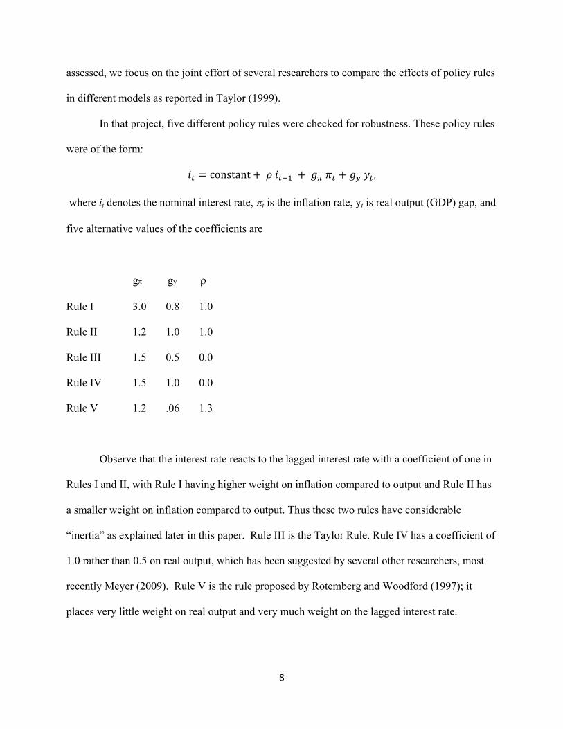
In that project, five different policy rules were checked for robustness. These policy rules

were of the form:

constant               ,

where it denotes the nominal interest rate, tis the inflation rate, yt is real output (GDP) gap, and

five alternative values of the coefficients are

g gy

Rule I 3.0 0.8 1.0

Rule II 1.2 1.0 1.0

Rule III 1.5 0.5 0.0

Rule IV 1.5 1.0 0.0

Rule V 1.2 .06 1.3

Observe that the interest rate reacts to the lagged interest rate with a coefficient of one in

Rules I and II, with Rule I having higher weight on inflation compared to output and Rule II has

a smaller weight on inflation compared to output. Thus these two rules have considerable

“inertia” as explained later in this paper. Rule III is the Taylor Rule. Rule IV has a coefficient of

1.0 rather than 0.5 on real output, which has been suggested by several other researchers, most

recently Meyer (2009). Rule V is the rule proposed by Rotemberg and Woodford (1997); it

places very little weight on real output and very much weight on the lagged interest rate.

9  

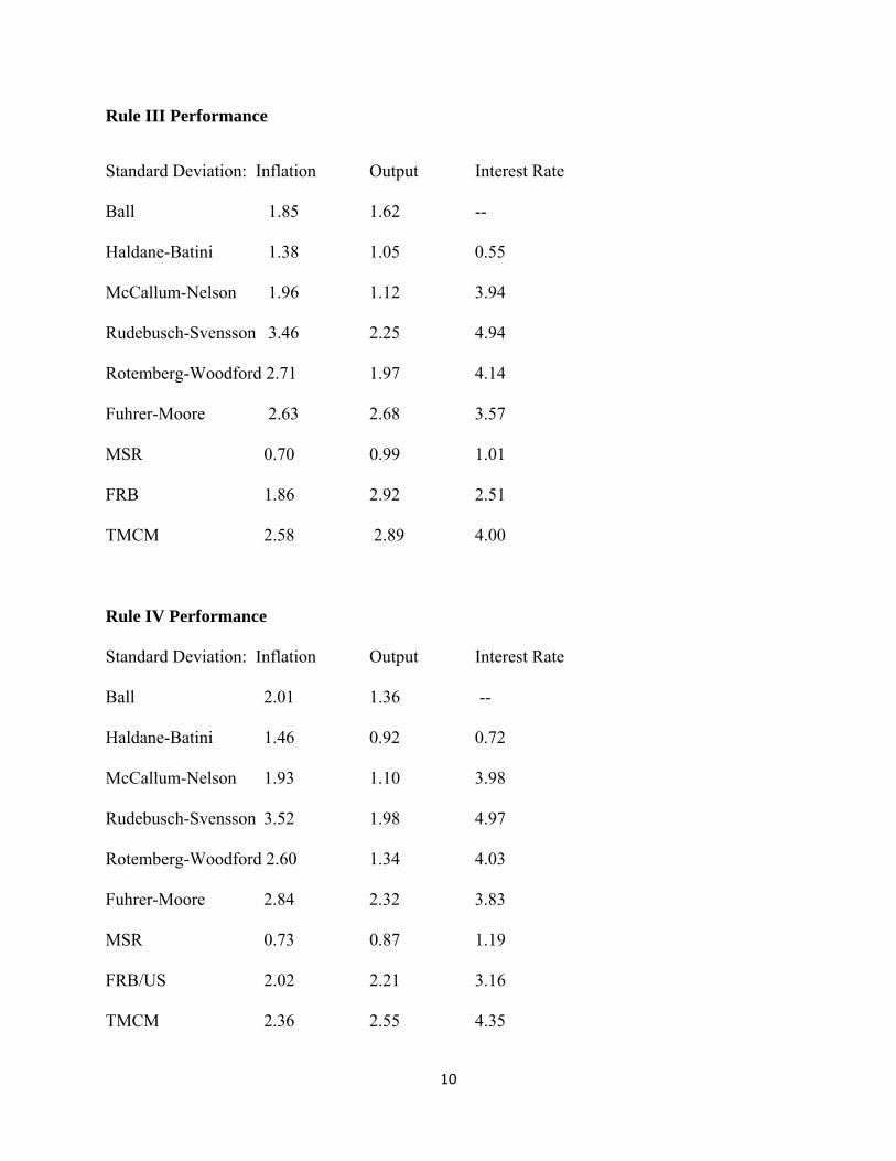
First consider the robustness of Rule III versus Rule IV. Recently several economists

have suggested that Rule IV is better than Rule III arguing that both the variability of inflation

and the variability of real output is lower with Rule IV than with Rule III. Is this finding robust

across models? Nine models were considered. To obtain details about the models see Taylor

(1993). For each of the models, the standard deviation of the inflation rate, of real output, and of

the interest rate for Rule III and Rule IV are shown below. Observe that the finding that Rule IV

dominates Rule III is not robust across models. For six of the nine models, Rule IV gives a

higher variance of inflation.

10  

Rule III Performance

Standard Deviation: Inflation Output Interest Rate

Ball 1.85 1.62 --

Haldane-Batini 1.38 1.05 0.55

McCallum-Nelson 1.96 1.12 3.94

Rudebusch-Svensson 3.46 2.25 4.94

Rotemberg-Woodford 2.71 1.97 4.14

Fuhrer-Moore 2.63 2.68 3.57

MSR 0.70 0.99 1.01

FRB 1.86 2.92 2.51

TMCM 2.58 2.89 4.00

Rule IV Performance

Standard Deviation: Inflation Output Interest Rate

Ball 2.01 1.36 --

Haldane-Batini 1.46 0.92 0.72

McCallum-Nelson 1.93 1.10 3.98

Rudebusch-Svensson 3.52 1.98 4.97

Rotemberg-Woodford 2.60 1.34 4.03

Fuhrer-Moore 2.84 2.32 3.83

MSR 0.73 0.87 1.19

FRB/US 2.02 2.21 3.16

TMCM 2.36 2.55 4.35

11  

Now consider the relative robustness of the three rules that respond to the lagged interest

rate (Rules I, II, and V). Using the same approach, Taylor (1999) reports that the sum of the

ranks of the three rules shows that Rule I is most robust if inflation fluctuations are the sole

measure of performance; it ranks first in terms of inflation variability for all but one model for

which there is a clear ordering. For output, Rule II has the best sum of the ranks, which reflects

its relatively high response to output. However, regardless of the objective function weights,

Rule V has the worst sum of the ranks of these three policy rules, ranking first for only one

model (the Rotemberg-Woodford model) in the case of output. Comparing rules I, II, III with

Rules III and IV) shows that the lagged interest rate rules do not dominate rules without a lagged

interest rate. For a number of models the rules with lagged interest rates are unstable or have

extraordinarily large variances.

The models that give very poor performance for the lagged interest rate rules are the ones

that have more lags and fewer leads. The reason is that they rely less on people’s forward-

looking behavior: if a small increase in the interest rate does not bring inflation down, then

people expect the central bank to raise interest rates by a larger amount in the future. But, in a

model without forward-looking, it is impossible to capture this behavior. Because Rule V has a

lagged interest rate coefficient greater than one, it greatly exploits these expectations effects and

is less robust than the other rules when evaluated without forward looking expectations.

3. Learning from Experience Before, During and After the Great Moderation

Another way to learn about the usefulness of simple policy rules is look at actual

macroeconomic performance when policy operates, or does not operate, close to such rules. The

12  

Great Moderation period is good for this purpose because economic performance was unusually

good in that period compared to the period before or, so far, the period after.

By all accounts the Great Moderation began in the early 1980s when the economy

became more stable. Not only did inflation and interest rates and their volatilities diminish

compared with the experience of the 1970s, but the volatility of real GDP reached lows never

seen before. Economic expansions became longer and stronger while recessions became

shallower and shorter. Many researchers have documented the improved cyclical performance

of the U.S. economy and pinpointed the date as starting sometime in the early 1980s. No matter

what metric you use—the variance of real GDP growth, the variance of the real GDP gap, the

average length of expansions, the frequency of recessions, or the duration of recessions—there

was a huge improvement in economic performance. There was also an improvement in price

stability with the inflation rate much lower and less volatile than the period from the late 1960s

to the early 1980s. This same type of improved performance occurred in other developed

countries. Research by Cecchetti and others (2006) shows this to be true for a broader group of

countries including most developing countries.

An easy way to date the start of the Great Moderation is the first month of expansion

following the 1981-82 recession or November 1982. Similarly one could date the end of the

Great Moderation in December 2007. That was the month of the start of what some call the

Great Recession which has been much more severe and much longer lasting than anything seen

during the Great Moderation. We may, of course, experience another Great Moderation (Great

Moderation II?) following the Great Recession, but for now let us say that Great Moderation I is

over.

13  

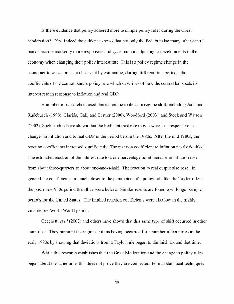
Is there evidence that policy adhered more to simple policy rules during the Great

Moderation? Yes. Indeed the evidence shows that not only the Fed, but also many other central

banks became markedly more responsive and systematic in adjusting to developments in the

economy when changing their policy interest rate. This is a policy regime change in the

econometric sense: one can observe it by estimating, during different time periods, the

coefficients of the central bank’s policy rule which describes of how the central bank sets its

interest rate in response to inflation and real GDP.

A number of researchers used this technique to detect a regime shift, including Judd and

Rudebusch (1998), Clarida, Gali, and Gertler (2000), Woodford (2003), and Stock and Watson

(2002). Such studies have shown that the Fed’s interest rate moves were less responsive to

changes in inflation and to real GDP in the period before the 1980s. After the mid 1980s, the

reaction coefficients increased significantly. The reaction coefficient to inflation nearly doubled.

The estimated reaction of the interest rate to a one percentage point increase in inflation rose

from about three-quarters to about one-and-a-half. The reaction to real output also rose. In

general the coefficients are much closer to the parameters of a policy rule like the Taylor rule in

the post mid-1980s period than they were before. Similar results are found over longer sample

periods for the United States. The implied reaction coefficients were also low in the highly

volatile pre-World War II period.

Cecchetti et al (2007) and others have shown that this same type of shift occurred in other

countries. They pinpoint the regime shift as having occurred for a number of countries in the

early 1980s by showing that deviations from a Taylor rule began to diminish around that time.

While this research establishes that the Great Moderation and the change in policy rules

began about the same time, this does not prove they are connected. Formal statistical techniques

14  

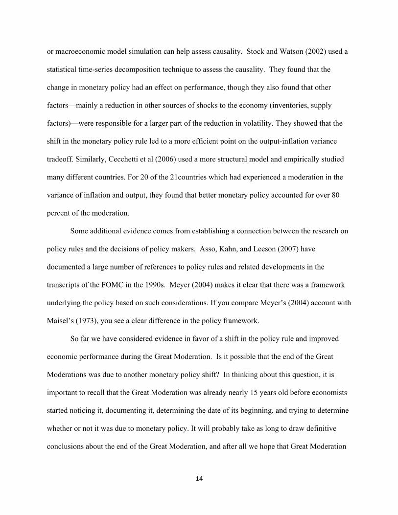
or macroeconomic model simulation can help assess causality. Stock and Watson (2002) used a

statistical time-series decomposition technique to assess the causality. They found that the

change in monetary policy had an effect on performance, though they also found that other

factors—mainly a reduction in other sources of shocks to the economy (inventories, supply

factors)—were responsible for a larger part of the reduction in volatility. They showed that the

shift in the monetary policy rule led to a more efficient point on the output-inflation variance

tradeoff. Similarly, Cecchetti et al (2006) used a more structural model and empirically studied

many different countries. For 20 of the 21countries which had experienced a moderation in the

variance of inflation and output, they found that better monetary policy accounted for over 80

percent of the moderation.

Some additional evidence comes from establishing a connection between the research on

policy rules and the decisions of policy makers. Asso, Kahn, and Leeson (2007) have

documented a large number of references to policy rules and related developments in the

transcripts of the FOMC in the 1990s. Meyer (2004) makes it clear that there was a framework

underlying the policy based on such considerations. If you compare Meyer’s (2004) account with

Maisel’s (1973), you see a clear difference in the policy framework.

So far we have considered evidence in favor of a shift in the policy rule and improved

economic performance during the Great Moderation. Is it possible that the end of the Great

Moderations was due to another monetary policy shift? In thinking about this question, it is

important to recall that the Great Moderation was already nearly 15 years old before economists

started noticing it, documenting it, determining the date of its beginning, and trying to determine

whether or not it was due to monetary policy. It will probably take as long to draw definitive

conclusions about the end of the Great Moderation, and after all we hope that Great Moderation

15  

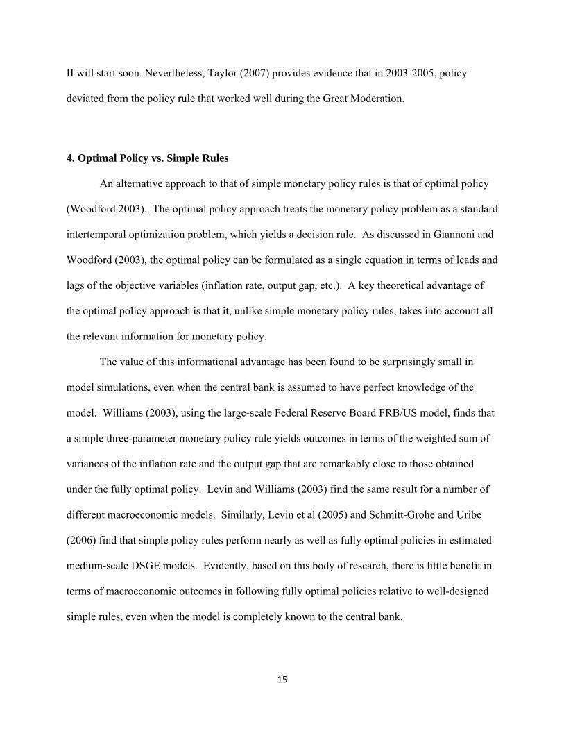
II will start soon. Nevertheless, Taylor (2007) provides evidence that in 2003-2005, policy

deviated from the policy rule that worked well during the Great Moderation.

 

4. Optimal Policy vs. Simple Rules

An alternative approach to that of simple monetary policy rules is that of optimal policy

(Woodford 2003). The optimal policy approach treats the monetary policy problem as a standard

intertemporal optimization problem, which yields a decision rule. As discussed in Giannoni and

Woodford (2003), the optimal policy can be formulated as a single equation in terms of leads and

lags of the objective variables (inflation rate, output gap, etc.). A key theoretical advantage of

the optimal policy approach is that it, unlike simple monetary policy rules, takes into account all

the relevant information for monetary policy.

The value of this informational advantage has been found to be surprisingly small in

model simulations, even when the central bank is assumed to have perfect knowledge of the

model. Williams (2003), using the large-scale Federal Reserve Board FRB/US model, finds that

a simple three-parameter monetary policy rule yields outcomes in terms of the weighted sum of

variances of the inflation rate and the output gap that are remarkably close to those obtained

under the fully optimal policy. Levin and Williams (2003) find the same result for a number of

different macroeconomic models. Similarly, Levin et al (2005) and Schmitt-Grohe and Uribe

(2006) find that simple policy rules perform nearly as well as fully optimal policies in estimated

medium-scale DSGE models. Evidently, based on this body of research, there is little benefit in

terms of macroeconomic outcomes in following fully optimal policies relative to well-designed

simple rules, even when the model is completely known to the central bank.

16  

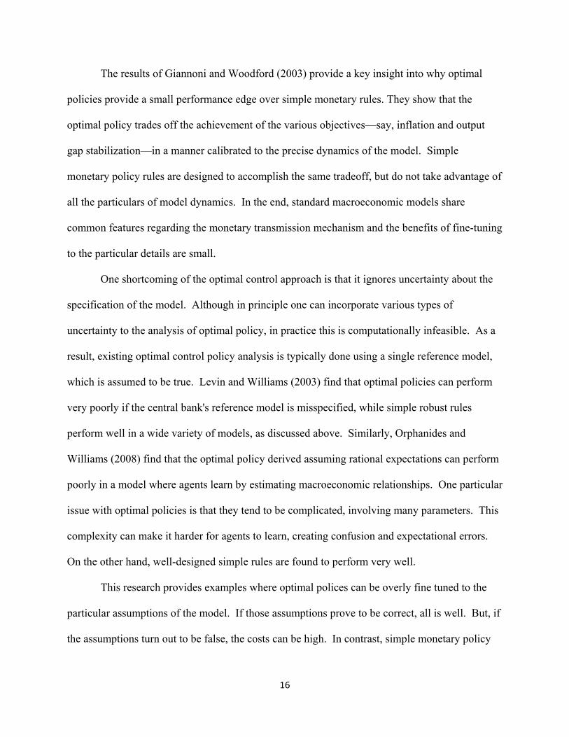
The results of Giannoni and Woodford (2003) provide a key insight into why optimal

policies provide a small performance edge over simple monetary rules. They show that the

optimal policy trades off the achievement of the various objectives—say, inflation and output

gap stabilization—in a manner calibrated to the precise dynamics of the model. Simple

monetary policy rules are designed to accomplish the same tradeoff, but do not take advantage of

all the particulars of model dynamics. In the end, standard macroeconomic models share

common features regarding the monetary transmission mechanism and the benefits of fine-tuning

to the particular details are small.

One shortcoming of the optimal control approach is that it ignores uncertainty about the

specification of the model. Although in principle one can incorporate various types of

uncertainty to the analysis of optimal policy, in practice this is computationally infeasible. As a

result, existing optimal control policy analysis is typically done using a single reference model,

which is assumed to be true. Levin and Williams (2003) find that optimal policies can perform

very poorly if the central bank's reference model is misspecified, while simple robust rules

perform well in a wide variety of models, as discussed above. Similarly, Orphanides and

Williams (2008) find that the optimal policy derived assuming rational expectations can perform

poorly in a model where agents learn by estimating macroeconomic relationships. One particular

issue with optimal policies is that they tend to be complicated, involving many parameters. This

complexity can make it harder for agents to learn, creating confusion and expectational errors.

On the other hand, well-designed simple rules are found to perform very well.

This research provides examples where optimal polices can be overly fine tuned to the

particular assumptions of the model. If those assumptions prove to be correct, all is well. But, if

the assumptions turn out to be false, the costs can be high. In contrast, simple monetary policy

17  

rules are designed to take account of only the most basic principle of monetary policy of leaning

against the wind of inflation and output movements. Because they are not fine tuned to specific

assumptions, they are more robust to mistaken assumptions.

5. Specific Issues

We now take up a number of specific issues related to the implementation of monetary

policy rules in practice. The first is the advantages and disadvantages of policy inertia, or

interest rate smoothing. The second concerns measurement issues. The third examines the

implications of the zero lower bound on interest rates.

Policy Inertia

One issue that has attracted considerable attention in the literature on monetary policy

rules is the role of policy inertia or interest rate smoothing in the rule.1 Inertia is typically

captured by including the lagged interest rate in the policy rule, as in the policy rules discussed

above. In models with forward-looking output and inflation, a high degree of policy inertia

creates a large, sustained movement in output gaps and inflation rates for a given movement in

the short-term interest rate (Levin, Wieland, and Williams 1999, Woodford 2003).2 Indeed, in

purely forward-looking models, the optimal coefficient on the lagged interest rate can exceed

unity.

However, in backward-looking models, a highly inertial rule can be disastrous because it

creates unstable cycles. In addition, “super inertial” rules with a lagged coefficient significantly

                                                            1 There has also been a large literature examining the presence of policy inertia in practice. See Sack and Wieland (2000), English, Nelson and Sack (2003), and Rudebusch (2006). 2 The presence of policy inertia is closely related to the effects of commitment for optimal policies. Dennis and Soderstrom (2006) find that the performance benefits of commitment over discretion are relatively in most empirical models.

18  

greater than unity perform poorly even in some forward-looking models. Levin and Williams

(2003) find that a monetary policy rule robust to a wide set of models is characterized by only a

modest degree of policy inertia. Schmitt-Grohe and Uribe (2006) and Edge et al (2009) find that

non-inertial rules perform very well in terms of household welfare in optimization-based

dynamic stochastic general equilibrium (DSGE) models.

Measurement issues

One practical issue that affects the implementation of monetary policy is the

measurement of variables of interest such as the inflation rate and the output gap (Orphanides

2001). Most macroeconomic data are subject to mismeasurement and revision. However,

measurement problems are particularly acute for the output gap, which depends on highly

uncertain estimates of a latent variable, potential output. This uncertainty encompasses that

resulting from estimating latent variables as well as uncertainty regarding the processes

influencing potential output (Orphanides and van Norden, 2002, Laubach and Williams 2003 and

Edge et al 2009). Similar problems plague estimation of related metrics such as the

unemployment gap or capacity utilization gap. The late 1960s and1970s were a period when

output and unemployment gap mismeasurement were arguably particularly severe. But, such

measurement problems have not been limited to that period, as difficulties in measuring gaps

extend into the present day (Orphanides et al 2002, Orphanides and Williams 2002).

A number of papers have examined the implications of measurement issues for monetary

policy rules (Orphanides et al 2000, Rudebusch 2001). A general finding is that the optimal

coefficient on the output gap declines in the presence of output gap mismeasurment. In these

papers, the level of potential output (of the natural rate of unemployment) is subject to persistent

19  

mismeasurement. When the output gap is mismeasured, a policy rule that responds to the change

in the gap, in addition to the level of the gap, performs better than a standard rule that responds

simply to the level of the output gap (Orphanides and Williams 2002). These policy rules that

respond more to the change in the gap take advantage of observation that the direction of the

change in the gap is generally less subject to mismeasurement than the absolute level of the gap

in the model simulations. In severe cases of mismeasurement, it can be optimal to replace

entirely the response to the output gap with a response to the change in the gap.

The zero lower bound

Up to this point, the discussion of monetary policy rules has abstracted from the zero

lower bound (ZLB) on nominal interest rates. Because there exists an asset, cash, that pays a

zero interest rate, it is not possible to for short-term nominal interest rates to fall significantly

below zero percent.3 In several instances—including the Great Depression in the United States,

Japan during the 1990s and much of the 2000s, and many countries during the most recession of

the late 2000s—the ZLB has constrained the ability of central banks to lower the interest rate in

the face of a weak economy and low inflation. This inability to reduce interest rates as low as

desired can impair the effectiveness of monetary policy to stabilize output and inflation.

The ZLB has three important implications for monetary policy rules. Assume that the

monetary policy rule is modified to account for the zero lower bound as follows:

max   0,       ,

where it is the short-term nominal interest rate, r* is the equilibrium real interest rate, πt is the

inflation rate, π* is the target inflation rate, and yt is the output gap. In the following, we refer to

                                                            3 Because cash is not a perfect substitute for bank reserves, the overnight rate can in principle be somewhat below zero, but there is a limit to how negative nominal interest rates can go as long as cash pays zero interest.

20  

the level of the policy rule that would obtain absent the ZLB (the value implied by the second

term in the bracket in the equation) as the unconstrained interest rate.

First, the ZLB can imply the existence of multiple steady states (Reifschneider and

Williams 2000, Benhabib, Schmitt-Grohe, and Uribe 2001). For a wide set of macroeconomic

models, one steady is characterized by a rate of inflation equal to the negative of the equilibrium

real interest rate, a zero output gap zero, and a zero nominal interest rate. Assuming the target

inflation rate exceeds the negative of the equilibrium real interest rate, a second steady state

exists. It is characterized by a rate of inflation equal to the central bank’s target inflation rate, a

zero output gap, and a nominal interest rate equal to the equilibrium real interest rate plus the

target inflation rate. In standard models, the steady state associated with the target inflation rate

is locally stable in the sense that the economy returns to this steady state following a small

disturbance. But, due to the existence of the ZLB, if a large contractionary shock hits the

economy, monetary policy alone may not be sufficient to bring the inflation rate back to the

target rate. Instead, depending on the nature of the model economy’s dynamics, the inflation rate

will either converge to the deflationary steady state or will diverge to infinitely negative inflation

rate. Fiscal policy can be used to eliminate the deflationary steady state and assure that the

economy returns to the desired steady state inflation rate (Evans, Guse, and Honkapohja, 2008).4

Second, the ZLB has implications for the specification and parameterization of the

monetary policy rule. For example, Reifschneider and Williams (2002) finds that increasing the

response to the output gap (value of α in the policy rule) helps reduce the effects of the ZLB.

Such an aggressive response to output gaps prescribes greater monetary stimulus before and after

episodes when the ZLB constrains policy, which helps lessen the effects when the ZLB

                                                            4 In addition to fiscal policy, researchers have examined the use of alternative monetary policy instruments, such as the quantity of reserves, the exchange rate, and longer-term interest rates. See Svensson (2001) and Bernanke and Reinhart (2004) for discussions of these topics.

21  

constrains policy. However, there are limits to this approach. First, it generally increases the

variability of inflation and interest rates, which may be undesirable. In addition, Williams

(2009) shows that too large a response to the output gap can be counterproductive. The ZLB

creates an asymmetry between the very strong responses to positive output gaps and truncated

responses to negative output gaps that increases output gap variability overall.

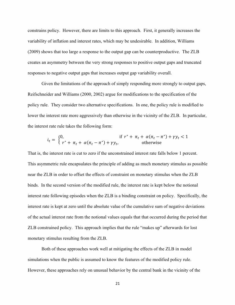
Given the limitations of the approach of simply responding more strongly to output gaps,

Reifschneider and Williams (2000, 2002) argue for modifications to the specification of the

policy rule. They consider two alternative specifications. In one, the policy rule is modified to

lower the interest rate more aggressively than otherwise in the vicinity of the ZLB. In particular,

the interest rate rule takes the following form:

 0,                                                       if       1       ,                       otherwise                          

That is, the interest rate is cut to zero if the unconstrained interest rate falls below 1 percent.

This asymmetric rule encapsulates the principle of adding as much monetary stimulus as possible

near the ZLB in order to offset the effects of constraint on monetary stimulus when the ZLB

binds. In the second version of the modified rule, the interest rate is kept below the notional

interest rate following episodes when the ZLB is a binding constraint on policy. Specifically, the

interest rate is kept at zero until the absolute value of the cumulative sum of negative deviations

of the actual interest rate from the notional values equals that that occurred during the period that

ZLB constrained policy. This approach implies that the rule “makes up” afterwards for lost

monetary stimulus resulting from the ZLB.

Both of these approaches work well at mitigating the effects of the ZLB in model

simulations when the public is assumed to know the features of the modified policy rule.

However, these approaches rely on unusual behavior by the central bank in the vicinity of the

22  

ZLB, which may confuse private agents and thereby entail unintended and potentially

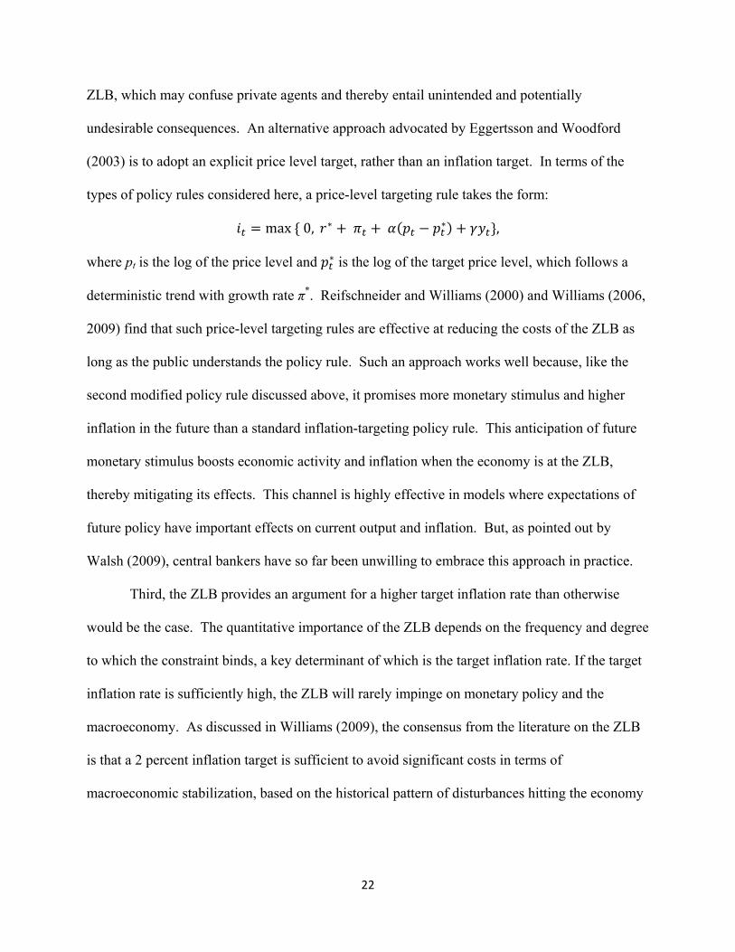
undesirable consequences. An alternative approach advocated by Eggertsson and Woodford

(2003) is to adopt an explicit price level target, rather than an inflation target. In terms of the

types of policy rules considered here, a price-level targeting rule takes the form:

max   0,       ,

where pt is the log of the price level and is the log of the target price level, which follows a

deterministic trend with growth rate π*. Reifschneider and Williams (2000) and Williams (2006,

2009) find that such price-level targeting rules are effective at reducing the costs of the ZLB as

long as the public understands the policy rule. Such an approach works well because, like the

second modified policy rule discussed above, it promises more monetary stimulus and higher

inflation in the future than a standard inflation-targeting policy rule. This anticipation of future

monetary stimulus boosts economic activity and inflation when the economy is at the ZLB,

thereby mitigating its effects. This channel is highly effective in models where expectations of

future policy have important effects on current output and inflation. But, as pointed out by

Walsh (2009), central bankers have so far been unwilling to embrace this approach in practice.

Third, the ZLB provides an argument for a higher target inflation rate than otherwise

would be the case. The quantitative importance of the ZLB depends on the frequency and degree

to which the constraint binds, a key determinant of which is the target inflation rate. If the target

inflation rate is sufficiently high, the ZLB will rarely impinge on monetary policy and the

macroeconomy. As discussed in Williams (2009), the consensus from the literature on the ZLB

is that a 2 percent inflation target is sufficient to avoid significant costs in terms of

macroeconomic stabilization, based on the historical pattern of disturbances hitting the economy

23  

over the past several decades. This figure is close to the inflation targets followed, either

explicitly or implicitly, by many central banks today (Kuttner 2004).

Asset prices and the monetary policy rule

Open economy models

Conclusion

To be written…

24  

References

Asso, Francesco, George Kahn, and Robert Leeson (2007) “Monetary Policy Rules: from Adam

Smith to John Taylor,” presented at Federal Reserve Bank of Dallas Conference, October

2007 http://dallasfed.org/news/research/2007/07taylor_leeson.pdf

Ball, Lawrence (1999) “Efficient Rules for Monetary Policy,” International Finance, Vol. 2, No.

1, pp. 63-83.

Benhabib, Jess, Stephanie Schmitt-Grohe, and Matin Uribe (2001), “The Perils of Taylor Rules,”

Journal of Economic Theory, 96(1-2), January, 40-69.  

Bernanke, Ben S., and Vincent R. Reinhart (2004), “Conducting Monetary Policy at Very Low

Short-Term Interest Rates,” American Economic Review, Papers and Proceedings, 94(2),

85-90.

Bryant, Ralph, Peter Hooper and Catherine Mann (1993), Evaluating Policy Regimes: New

Empirical Research in Empirical Macroeconomics, Brookings Institution, Washington,

D.C.

Cecchetti, Stephen G., Alfonso Flores-Lagunes, and Stefan Krause (2006) “Has Monetary Policy

Become More Efficient? A Cross-country Analysis” Economic Journal, Vol. 116, No.

115, pp. 408-433.

Cecchetti, Stephen G., Peter Hooper, Bruce C. Kasman, Kermit L. Schoenholtz, and Mark W.

Watson (2007), “Understanding the Evolving Inflation Process,” presented at the U.S.

Monetary Policy Forum 2007.

Clarida, Richard, Jordi Gali, and Mark Gertler (2000), “Monetary Policy Rules and

Macroeconomic Stability: Evidence and Some Theory,” Quarterly Journal of Economics

(February), 115, 1, 147-180.

25  

Coenen , Guenter, Athansios Orphanides, and Volker Wieland (2004), “Price Stability and

Monetary Policy Effectiveness when Nominal Interest Rates are Bounded at Zero,”

Advances in Macroeconomics, 4(1).

Dennis, Richard and Ulf Soderstrom (2006), “How Important Is Precommitment for Monetary

Policy?” Journal of Money, Credit, and Banking, 38(4), June, 847-872.

Edge, Rochelle M., Thomas Laubach, and John C. Williams (2009), “Welfare-Maximizing

Monetary Policy under Parameter Uncertainty,” Journal of Applied Econometrics,

forthcoming.

Eggertsson, Gauti B., and Michael Woodford (2003), “The Zero Interest-Rate Bound and

Optimal Monetary Policy,” Brookings Papers on Economic Activity, 1, 139-211.

Eggertsson, Gauti B., and Michael Woodford (2006), ``Optimal Monetary and Fiscal Policy in a

Liquidity Trap,” NBER International Seminar on Macroeconomics 2004, Richard H.

Clarida, Jeffrey Frankel, Francesco Giavazzi and Kenneth D. West, eds., Cambridge,

MA.: MIT Press, 75-131.

English, William B., William R. Nelson, and Brian Sack (2003), “Interpreting the Significance

of the Lagged Interest Rate in Estimated Monetary Policy Rules,” Contributions to

Macroeconomics, 3.

Evans, George W., Eran Guse, and Seppo Honkapohja (2008), “Liquidity Traps, Learning and

Stagnation,” European Economic Review, 52, 1438 – 1463.

26  

Giannoni, Marc P. and Michael Woodford (2005), “Optimal Inflation Targeting Rules,'' In:

Bernanke, B.S., Woodford, M. (Eds.), The Inflation Targeting Debate, Chicago:

University of Chicago Press, 93—162.

Judd, John and Glenn D. Rudebusch (1998). "Taylor's Rule and the Fed: 1970-1997." Federal

Reserve Bank of San Francisco Economic Review 3, pp. 1-16.

Laubach, Thomas and John C. Williams (2003), “Measuring the Natural Rate of Interest,”

Review of Economics and Statistics, 85(4), November, 1063-1070.

Kuttner, Kenneth N. (2004), “A Snapshot of Inflation Targeting in its Adolescence,” in

Christopher Kent and Simon Guttmann (ed.), The Future of Inflation Targeting, Sydney,

Australia: Reserve Bank of Australia, November, 6-42.

Levin, Andrew T., Alexei Onatski, John C. Williams, and Noah Williams (2005), “Monetary

Policy Under Uncertainty in Micro-Founded Macroeconometric Models,” NBER

Macroeconomics Annual 2005, 229-289.

Levin, Andrew, Volker Wieland, and John C. Williams (1999), "Robustness of Simple Monetary

Policy Rules under Model Uncertainty." In Monetary Policy Rules, John B. Taylor (Ed),

pp. 263-299. Chicago: Chicago University Press.

Levin, Andrew T. and John C. Williams (2003), “Robust Monetary Policy with Competing

Reference Models,” Journal of Monetary Economics, 50, 945--975.

Maisel, Sherman J. (1973), Managing the Dollar, W.W. Norton, New York.

27  

McCallum, Bennett (1999) “Issues in the Design of Monetary Policy Rules,” Handbook of

Macroeconomics, John B. Taylor and Michael Woodford (eds).

McCallum, Bennett T., “Theoretical Analysis Regarding a Zero Lower Bound on Nominal

Interest Rates,” Journal of Money, Credit and Banking, 32(4), November 2000.

Meyer, Laurence (2009), “Dueling Taylor Rules,” unpublished paper, August.  

Meyer, Laurence (2004), A Term at the Fed: An Insider’s View, HarperCollins, New York. 

Mishkin, Frederick (2007), “Housing and the Monetary Policy Transmission Mechanism,”

Federal Reserve Bank of Kansas City, Jackson Hole Conference.

Orphanides, Athanasios, and others (2000), “Errors in the Measurement of the Output Gap and

the Design of Monetary Policy,” Journal of Economics and Business, 52(1-2), 117–41.

Orphanides, Athanasios and Simon van Norden (2002), “The Unreliability of Output Gap

Estimates in Real Time,” Review of Economics and Statistics, 84(4), 569-583, November.

Orphanides, Athanasios and John C. Williams (2008) “Learning, Expectations Formation, and

the Pitfalls of Optimal Control Monetary Policy,” Journal of Monetary Economics, Vol.

55S, pp. S80-S96, October.  

Reifschneider, David L. and John C. Williams (2000), “Three Lessons for Monetary Policy in a

Low Inflation Era,” Journal of Money, Credit and Banking, 32(4), November, 936-966. 

Reifschneider, David L. and John C. Williams (2002), “FOMC Briefing,” Board of Governors

of the Federal Reserve System, January.

Romer, Christina D., and David H. Romer (2002), “A Rehabilitation of Monetary Policy in The

1950's,” American Economic Review, 92(2), May, 121-127.

28  

Rotemberg, Julio and Michael Woodford (1997), “An Optimization-Based Econometric

Framework for the Evaluation of Monetary Policy,” NBER Macroeconomics Annual, Ben

S. Bernanke and Julio Rotemberg (Eds.) pp. 297 – 361.  

Rudebusch, Glenn D. (2001), “Is the Fed Too Timid? Monetary Policy in an Uncertain World.”

Review of Economics and Statistics, 83, May, pp. 203-217.

Rudebusch, Glenn D. (2006), “Monetary Policy Inertia: Fact or Fiction?” International Journal

of Central Banking, 2(4), December, 85-135.

Sack, Brian and Volker Wieland (2000), “Interest-Rate Smoothing and Optimal Monetary

Policy: A Review of Recent Empirical Evidence,” Journal of Economics and Business,

January.

Schmitt-Grohe, Stephanie and Martin Uribe (2006), “Optimal Simple and Implementable

Monetary and Fiscal Rules,” Journal of Monetary Economics.

Stock, James and Mark Watson (2002), “Has the Business Cycle Changed,” in Monetary Policy

and Uncertainty: Adapting to a Changing Economy, Jackson Hole Conference, Federal

Reserve Bank of Kansas City, pp 9-56.

Svensson, Lars E.O. (2001), “The Zero Bound in an Open Economy: A Foolproof Way of

Escaping from a Liquidity Trap,” Monetary and Economic Studies, 19(S-1), February,

277-312.

Taylor, John B. (1979), “Estimation and Control of a Macroeconomic Model with Rational

Expectations,” Econometrica, 47, September 1979.

Taylor, John B. (1999), Monetary Policy Rules, (Editor), University of Chicago Press

Taylor, John B. (2007), ``Housing and Monetary Policy,'' In: Housing, Housing Finance, and

Monetary Policy, Kansas City, MO: Federal Reserve Bank of Kansas City, 463-476.

29  

 Tetlow, Robert J. (2006), “Real-time Model Uncertainty in the United States: ‘Robust’ policies

put to the test,” mimeo, Federal Reserve Board, May 22.

Taylor, John B. (2009) “Surprising Comparative Properties of Monetary Models: Results from a

New Monetary Model Database,” Paper presented at the Econometric Society Meetings,

San Francisco, January.

Walsh, Carl (2009), “Using monetary policy to stabilize economic activity,” Federal Reserve

Bank of Kansas City, Jackson Hole Conference.

Williams, John C. (2003), “Simple Rules for Monetary Policy,” Federal Reserve Bank of San

Francisco Economic Review, 2003.

Williams, John C. (2006), “Monetary Policy in a Low Inflation Economy with Learning,” in:

Monetary Policy in an Environment of Low Inflation; Proceedings of the Bank of Korea

International Conference 2006, Seoul: Bank of Korea, 199-228.

Williams, John C. (2009), “Heeding Daedalus: Optimal Inflation and the Zero Lower Bound,”

prepared for Brookings Papers on Economic Activity, September 2009.

Woodford, Michael (2001), “The Taylor Rule and Optimal Monetary Policy,” American

Economic Review, Papers and Proceedings, Vol. 91, No. 2, pp. 232-7.

Woodford, Michael (2003), Interest and Prices, Princeton, NJ: Princeton University Press.