simpliﬁed evaporation method for determining soil ... · pdf fileauthor's personal copy...

Author's personal copy

Simplified evaporation method for determining soil

hydraulic properties

A. Peters *, W. Durner

Institute of GeoEcology, Department of Soil Science and Soil Physics, Braunschweig Technical University, Germany

Received 26 September 2007; received in revised form 4 March 2008; accepted 3 April 2008

KEYWORDS

Hydraulic properties;Evaporation experiment;Soil water flow;Richards equation;Parameter optimization

Summary Evaporation experiments are commonly used to derive hydraulic properties ofsoils. In the simplified evaporation method, as proposed by Schindler [Schindler, U., 1980.Ein Schnellverfahren zur Messung der Wasserleitfahigkeit im teilgesattigten Boden an Ste-chzylinderproben. Arch. Acker- u. Pflanzenbau u. Bodenkd. Berlin 24, 1–7], the weight ofa soil sample and pressure heads at two height levels are recorded at consecutive times.The evaluation of these measurements relies on linearization assumptions with respect totime, space and the water content–pressure head relationship. In this article, we inves-tigate the errors that result from the linearization assumptions, and show how systematicand stochastic measurement errors affect the calculation of water retention and hydraulicconductivity data and the resulting fits of soil hydraulic functions. We find that lineariza-tion errors with respect to time are negligible if cubic Hermite splines are used for datainterpolation. Linearizations in space lead to minor errors, even in the late stage of evap-oration where strongly non-linear pressure head profiles emerge. A bias in the estimatedretention function results from the negligence of a non-linear water content distributionin the sample at the begin of the evaporation process, and affects primarily coarse sandsor soils with structured pore systems. This error can be avoided if an integral evaluation ofthe measurements is used. We introduce an applicable rejection criterion for unreliablehydraulic conductivity data near saturation, based on the error in the hydraulic gradient.Calibration errors of tensiometers lead to biased estimates of hydraulic properties in thewet range, whereas errors in tensiometer installation positions yield biases in the dryrange. Random errors in data cause no significant bias, and parametric hydraulic functionscan be estimated with small uncertainties, if water retention and conductivity functionsare coupled and the underlying model structure is correct.ª 2008 Elsevier B.V. All rights reserved.

0022-1694/$ - see front matter ª 2008 Elsevier B.V. All rights reserved.doi:10.1016/j.jhydrol.2008.04.016

* Corresponding author. Tel.: +49 5315930; fax: +49 5315637.E-mail address: [email protected] (A. Peters).

Journal of Hydrology (2008) 356, 147–162

ava i lab le a t www.sc iencedi rec t . com

journal homepage: www.elsevier .com/ locate / jhydrol


Introduction

Modeling water and solute transport in the unsaturated soilby means of the Richards equation requires an accurateknowledge of the water retention function, hðhÞ, and thehydraulic conductivity function, KðhÞ, where h is the volu-metric water content, K ðcm dÿ1Þ is the hydraulic conduc-tivity and h ðcmÞ is the pressure head. These soil hydraulicproperties may be obtained by a variety of methods (vanGenuchten et al., 1999; Durner and Lipsius, 2005). Mostwidely used are hydrostatic column experiments to derivehðhÞ (Dane and Hopmans, 2002) and the estimation of KðhÞfrom hðhÞ by capillary bundle models like Mualem’s integral(Mualem, 1976). Alternatively, transmission and capacityparameters can be determined simultaneously, e.g., by aseries of steady-state experiments (Bouma et al., 1983;Dirksen, 1991; Durner and Lipsius, 2005), but the time de-mand for this method becomes prohibitively large for lowerwater contents. Most suitable is therefore the evaluation oftransient flow experiments, such as multi-step inflow/out-flow experiments (Durner et al., 1999) or evaporationexperiments (Wind, 1968; Simunek et al., 1998a).

The numerical inversion of transient flow experiments isthemost accurate way to determine soil hydraulic properties(Simunek et al., 1998a; Romano and Santini, 1999; Hopmanset al., 2002), but the numerical inversion has disadvantagessuch as the high computational burden and problems withthe numerical solution of the forward problem in the inverseframework (Durner et al., 1999). Therefore, simplifyingmethods that depend on certain linearizing assumptions areattractive and widely applied. The most popular way to eval-uate evaporation experiments is Wind’s method (Wind,1968), which was later automated (Boels et al., 1978;Halbertsma and Veerman, 1994) and further simplified(Schindler, 1980; Wendroth et al., 1993).

In transient evaporation experiments, both the verticaldistributions of the water contents and pressure heads,and their temporal evolution are in general non-linear. How-ever, they can be linearly approximated (Wind, 1968; Schin-dler, 1980). At the beginning of the experiment the pressurehead profile is linear (Romano and Santini, 1999) and theevaporation rate is given by the atmospheric demand ofthe laboratory air. In this first stage the evaporation rateremains accordingly almost constant because the decreasein unsaturated hydraulic conductivity due to water loss issufficiently compensated by an increase of the hydraulicgradient. In the second stage, the evaporation rate gradu-ally decreases with time (Kutilek and Nielsen, 1994) andboth the pressure head and water content profile in thesample become non-linear. Among the different evaluationmethods for evaporation experiments, the method proposedby Schindler (1980) is particularly attractive due to its sim-plicity, easy computation and small data demand. It relieson pressure head measurements in only two depths andthe total column weights recorded at several times, thusassuming that all non-linearities are small and that the er-rors introduced by the linearizations are negligible.

The aim of this article is to evaluate the accuracy and theuncertainties of the simplified evaporation method bySchindler (1980), for soils of various texture and structureand to improve the method. In a sensitivity analysis we

investigate the type and magnitude of systematic errorsthat are introduced by the linearization assumptions andwe show how errors in the calibration and position of thetensiometers and uncertainties in the measurement affectthe results, similar to Mohrath et al. (1997) and Bertuzziet al. (1999) for the original Wind method. We show howthe temporal linearization errors can be diminished by useof cubic hermite spline interpolation. Furthermore, our sub-sequent parameter estimation procedure accounts for thenon-linear water content distribution in the first stage ofthe experiment and thus eliminates one of the systematicerrors of the classic evaluation close to saturation. This isof particular relevance for structured soils with a secondarypore system due to aggregation (Coppola, 2000; Spohrer etal., 2005) or soils with multiple pore-density maxima (Mal-lants et al., 1997), which require bimodal or multimodalretention functions (Othmer et al., 1991; Durner, 1994) orfree-form functions (Bitterlich et al., 2004; Iden and Dur-ner, 2007). Since the estimation of KðhÞ is very uncertainat low hydraulic gradients (Wendroth et al., 1993; Tamariet al., 1993) we introduce a rejection criterion for KðhÞ datadepending on the error in the hydraulic gradient.

Materials and methods

Simplified evaporation method

In a typical evaporation experiment, pressure heads at mul-tiple heights and column weights are taken at a number oftimes, until either the tensiometers used for pressure headreadings fail, or the weight change becomes negligible (Pla-gge et al., 1999; Halbertsma and Veerman, 1994). UnlikeWind’s approach (Wind, 1968), the simplified method ofSchindler uses pressure head measurements, h1 and h2, atonly two different depths, z1 ðcmÞ and z2 ðcmÞ (Schindler,1980). The mean water content, �hi, derived from the col-umn weight, and the mean pressure head, �hi, are evaluatedat each time step i to get data for the retention function.Since Schindler proposed to place the two tensiometers atheights z1 ¼ 0:25L and z2 ¼ 0:75L, where L ðcmÞ is theheight of the column, �hi is calculated simply as arithmeticmean of the two measured values.

The water flow between two times tiÿ1 and ti through aplane, which is located exactly at the center between thetwo tensiometric measurement levels, is assumed to beequal to qi ¼ zm � Dhi=Dti, where Dhi ¼ �hi ÿ �hiÿ1 is the meanwater content change between the readings, caused by theevaporation loss through the surface, Dti ¼ ti ÿ tiÿ1 is thetime increment between two readings and zm ðcmÞ is the dis-tance from the bottom of the column to the plane betweenthe two tensiometers. The data for the hydraulic conductiv-ity function are derived by inverting Darcy’s law:

K ið��hiÞ ¼ ÿ qi

Dhi=Dzþ 1; ð1Þ

where ��hi is the mean pressure head between time step i andiÿ 1 for the two depths, K i is the hydraulic conductivity cor-responding to ��hi, Dhi is the mean difference between thetensiometer readings and Dz ¼ z2 ÿ z1 is the distance be-tween the tensiometers. In the symmetric experimental set-up of Schindler, ��hi ¼ 0:25 � ðhiÿ1

1 þ hiÿ12 þ h

i1 þ h

i2Þ and Dhi ¼

148 A. Peters, W. Durner


0:5 � ððhiÿ12 ÿ h

iÿ11 Þ þ ðhi

2 ÿ hi1ÞÞ where the subscripts indicate

the spatial position and the superscripts the time steps.

Correcting for non-linearity in hðzÞ

The simplified method assumes that the vertical water con-tent and pressure head distributions are linear over thewhole column, and not only over small sections of the col-umn, as in Wind’s original method. For physical reasons, thisassumption can be only approximately fulfilled. First, thehydraulic gradient must be larger toward the soil surfacesince the water flux density increases and the hydraulicconductivity decreases with increasing distance from theimpermeable bottom boundary. Second, the water contentis usually a non-linear function of the pressure head.

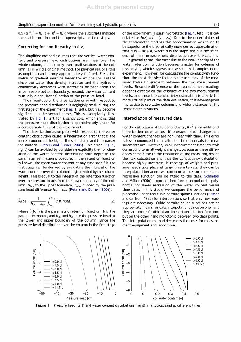
The magnitude of the linearization error with respect tothe pressure head distribution is negligibly small during thefirst stage of the experiment (Fig. 1, left), but may becomesignificant in the second phase. This is exemplarily illus-trated by Fig. 1, left for a sandy soil, which shows thatthe pressure head distribution is approximately linear fora considerable time of the experiment.

The linearization assumption with respect to the watercontent distribution causes a linearization error that is themore pronounced the higher the soil column and the coarserthe material (Peters and Durner, 2006). This error (Fig. 1,right) can be avoided by considering explicitly the non-line-arity of the water content distribution with depth in theparameter estimation procedure. If the retention functionis known, the mean water content at any time step i in thefirst stage can be derived by evaluating the integral of thewater contents over the column height divided by the columnheight. This is equal to the integral of the retention functionover the pressure heads from the lower boundary of the col-umn, hlbi , to the upper boundary, hubi, divided by the pres-sure head difference hlbi ÿ hubi (Peters and Durner, 2006):

�hiðbÞ ¼

1

hlbi ÿ hubi

Z hubi

hlbi

hðb; hÞdh; ð2Þ

where hðb; hÞ is the parametric retention function, b is theparameter vector, and hlbi and hubi are the pressure head atthe lower and upper boundary of the column. Since thepressure head distribution over the column in the first stage

of the experiment is quasi-hydrostatic (Fig. 1, left), it is cal-culated as hðzÞ ¼ �hÿ ðzÿ zmÞ. Due to the uncertainties ofthe tensiometer readings this approximation was found tobe superior to the theoretically more correct approximationthat hðzÞ ¼ azþ b, where a is the slope and b is the inter-cept of linear pressure head distribution over the column.

In general terms, the error due to the non-linearity of thewater retention function becomes smaller for columns ofless height, which suggests to use small soil samples in theexperiment. However, for calculating the conductivity func-tion, the most decisive factor is the accuracy of the mea-sured hydraulic gradient between the two measurementlevels. Since the difference of the hydraulic head readingsdepends directly on the distance of the two measurementlevels, and since the conductivity estimation is clearly themore critical part of the data evaluation, it is advantageousin practice to use taller columns and wider distances for thetensiometer positions.

Interpolation of measured data

For the calculation of the conductivity, K ið��hiÞ, an additionallinearization error arises, if pressure head changes andwater content changes are non-linear with time. This erroris less pronounced the smaller the time intervals for mea-surements are. However, small measurement time intervalscorrespond to small weight changes. As soon as these differ-ences come close to the resolution of the measuring devicethe flux calculation and thus the conductivity calculationbecome highly uncertain. If readings of weights and pres-sure heads take place at large time intervals, they can beinterpolated between two consecutive measurements or aregression function can be fitted to the data. Schindlerand Muller (2006) proposed therefore a second order poly-nomial for linear regression of the water content versustime data. In this study, we compare the performance ofpiecewise linear and cubic hermite spline functions (Fritschand Carlson, 1980) for interpolation, so that only few read-ings are necessary. Cubic hermite spline functions are anappropriate means for data interpolation, since on one handthey are more flexible than linear interpolation functionsbut on the other hand monotonic between two data points.This interpolation method decreases the costs for measure-ment equipment and labor time.

–50 –40 –30 –20 –10 0–6

–5

–4

–3

–2

–1

0

Co

lum

n d

ep

th [

cm

]

Pressure head [cm]

t=0.0 dt=1.5 dt=3.0 dt=4.5 dt=6.0 dt=7.5 dt=9.0 dt=11.5 d

0 0.1 0.2 0.3 0.4 0.5–6

–5

–4

–3

–2

–1

0

Co

lum

n d

ep

th [

cm

]

Vol. water content [–]

t=0.0 dt=1.5 dt=3.0 dt=4.5 dt=6.0 dt=7.5 dt=9.0 dt=11.5 d

Figure 1 Pressure head (left) and water content distributions (right) in a typical sand at different times.

Simplified evaporation method for determining soil hydraulic properties 149


Fit of parametric expressions to the hðhÞ and KðhÞdata

To be used in numerical simulation models of water trans-port, parametric models for hðhÞ and KðhÞ are fitted tothe data by a non-linear regression algorithm by minimizinga measure of misfit. In this work, we fit the coupled K–h–h

model of van Genuchten/Mualem (van Genuchten, 1980)or the bimodal model of Durner/Mualem (Durner, 1994) tothe measured data, by minimizing the sum of weightedsquared residuals between model prediction and data pairs:

UðbÞ ¼ wh

Xr

i¼1

whi ½�hi ÿ hiðbÞ�2 þ wK

Xk

i¼1

wK i½K i ÿ bK iðbÞ�2; ð3Þ

where r and k are the number of data pairs for the retentionfunction and the conductivity function, respectively, wh andwK are the class weights of the water content data and con-ductivity data, whi and wKi

are the weights of the individualdata points, and �hi, hiðbÞ, K i and bK iðbÞ are the measured andmodel predicted values, respectively. In Eq. (3), the pre-dicted water contents, h, are either calculated in a standardmanner as the point water contents at pressure head �hi

(‘‘classic method’’), or as the mean water content of thewhole column, as given by Eq. (2) (‘‘integral method’’).

Since the objective function, UðbÞ, involves data of dif-ferent types with different measurement frequency, theresult of the optimization will likely be affected by theweights of the data (Simunek and Hopmans, 2002). There-fore, we normalized the weights first by a factor for thedata type and second by a factor for the data frequency.To account for the different measurement frequency, theindividual weights, whi and wKi

were chosen such that thecombined data within every log10ðÿhÞ ð� pF) incrementhave the same weight, i.e., the weight for a certain datapoint was proportional to its distance to the neighboringpoint on the pF scale. To account additionally for the differ-ent data types, the weights for the data classes were calcu-lated by wh ¼ 1=ðhmax ÿ hminÞ and wk ¼ 1=ðlog10ðKmaxÞÿlog10ðKminÞÞ, where hmax, hmin, Kmax and Kmin are the maxi-mum and minimum values of the data sets to be fitted.

As fitting procedure we use a robust combination of theshuffled complex evolution (SCE-UA) algorithm with aLevenberg–Marquardt (LM) algorithm. The SCE-UA algo-rithm (Duan et al., 1992), is a global optimizer and con-verges within pre-defined permissible parameter rangestoward the minimum (if that exists), not depending on ini-tial guesses. The Levenberg–Marquardt (LM) algorithm isan efficient local optimizer (Marquardt, 1963). It is usedto speed up the convergence, once the close region of theglobal optimum is identified by the SCE. A similar approach,combining a global with a local optimizer, for the estima-tion of soil hydraulic properties was introduced by Lambotet al. (2002).

Forward modeling of evaporation scenarios

Modeling scenario

To analyze the type and magnitude of errors that are in-duced by the linearization assumptions of the evaporationmethod, and by different types of measurement errors,we performed a sensitivity analysis with synthetic measure-

ments for an evaporation experiment with a constantpotential evaporation rate and four types of soils. The soilhydraulic properties were expressed by the uni- and bimodalconstrained van Genuchten expression for the retentionfunction and Mualem’s predictive model for the conductiv-ity function. The retention function is given by

SeðhÞ ¼Xk

i¼1

wiSei ; ð4Þ

where Se ¼ ðhÿ hrÞ=ðhs ÿ hrÞ is the effective saturation, Seiare weighted sub-functions of the system, wi are theweighting factors for the sub-functions, subject to0 < wi < 1 and

Pwi ¼ 1, and hr and hs are the residual

and the saturated water contents. The effective satura-tions, Sei are given by

SeiðhÞ ¼ ð1þ ðaijhjÞniÞ1=niÿ1; ð5Þwhere ai (cm

ÿ1) and ni are curve-shape parameters of pore-subsystems. For k ¼ 1, Eq. (4) represents the retentioncurve of van Genuchten (1980), for k ¼ 2 the bimodal reten-tion function by Durner (1994).

The relative unsaturated hydraulic conductivity function,KrðhÞ, as used in this study, is calculated from soil waterretention characteristic according to Mualem (1976)

KrðSeðhÞÞ ¼ Sse

R Se

0hÿ1 dSeðhÞR 1

0hÿ1 dSeðhÞ

" #2

; ð6Þ

where s is a factor accounting for tortuosity that has in theoriginal publication of Mualem a value of 0.5. FollowingHoffmann-Riem et al. (1999) and Schaap and Leij (2000),we treat s as a free fitting parameter. To evaluate Eq.(6), the analytical solutions of van Genuchten (1980) andPriesack and Durner (2006) were used.

Evaporation from a vertical soil column was simulated bysolving the Richards equation with the constitutive relation-ships as described by Eqs. (4)–(6) using the finite elementcode HYDRUS-1D (Simunek et al., 1998b). The height ofthe simulated column was 6.0 cm. At the lower boundarya no-flux boundary condition was applied,

ÿKdh

dzþ 1

� �¼ 0: ð7Þ

and at the upper boundary a flux boundary condition waschosen:

ÿKdh

dzþ 1

� �¼ q0; ð8Þ

where q0 was 0:2 cm dÿ1. This flux was maintained until thepressure head at the upper boundary reached a value ofÿ105 cm. After the head met that value, the boundary con-dition was changed toward a Dirichlet condition and thusthe evaporation rate became non-linear, indicating thebeginning of the second stage of the experiment. The massbalance error in the forward simulations was in all casessmaller than 0.5%.

Three unimodal soils, representing a typical sand (S),loam (L) or clay (C) were used. The parameters for thehydraulic properties were obtained with the neural networkprogram ROSETTA (Schaap et al., 1998) assuming typicaltextures and bulk densities for the tested soils. As a fourth



soil, bimodal hydraulic functions that represent a structuredclay (BI) soil were chosen. The soil hydraulic parameters ofthe four cases are listed in Table 1.

Generation of synthetic data

To obtain synthetic pressure head measurements that couldbe used together with the cumulative outflow as input datafor the simplified evaporation method, the pressure headswere read at 1.5 and 4.5 cm underneath the surface. Theresulting data were analyzed either until the matric headat the upper tensiometer position reached ÿ1000 cm, whichis the typical measurement limit for tensiometers, or untilthe weight change became negligible (for the sand after15 d). The ‘‘measurements’’ were taken in different tempo-ral resolutions (0.1–3 d) and were interpolated piecewiselinear (plin) or by cubic hermite spline functions (spline).From the interpolated functions 100 data were selectedthat were equally distributed on a

ffiffit

paxis.

In order to investigate the error caused purely by the lin-earization assumptions, we first created data without anyadditional error. In a second part, we investigated the errorthat results from a bias in the tensiometer calibration. Forthis, constant offsets of ÿ1, 0 and 1 cm in the reading ofthe upper tensiometer were imposed. In the third part theposition of the upper tensiometer was varied to be ÿ0.42,0 and 0.42 cm off from the correct plane to investigatethe effects caused by erroneous tensiometer positions. Ina fourth part, the influence of stochastic measurementerrors was investigated. Thus, the positions and thecalibrations were assumed to be correct, but a normal dis-tributed noise with zero mean and standard deviationrh ¼ 0:2 cm was imposed on the tensiometer readings. Inthese simulations, the weight measurements were also per-turbed with a normal distributed random error with a stan-dard deviation rw ¼ 0:02 g (i.e. 4:8� 10ÿ4 cm for the onedimensional case if the height and volume of the columnare 6 cm and 250 cm3, respectively). Both errors representtypical uncertainties of laboratory measurements. To getreliable results on how this random measurement errors af-fect the calculations, 500 realizations were created andevaluated.

Data evaluation

The synthetically created data were analyzed with the sim-plified evaporation method to derive data pairs for the hðhÞand KðhÞ-functions. Due to limited accuracy of tensiometricmeasurements, the calculation of KðhÞ at small hydraulichead gradients becomes highly uncertain (Wendroth et al.,1993; Tamari et al., 1993). Thus, all calculations of K datafor gradients smaller than a certain threshold value, asspecified in the results section, were rejected in this study.

The remaining data pairs were considered reliable, and thewater retention curve and the related conductivity curvewere fitted by minimizing Eq. (3). All parameters were esti-mated simultaneously. Thus, for the unimodal soils sixparameters (hs, hr, a, n, Ks and s) and for the bimodal casenine parameters (hs, hr, a1, n1, a2, n2, w2, Ks and s) werefitted.

Diagnostic variables

To quantify the maximum error introduced by the lineariza-tion assumptions and the various error sources, the maxi-mum deviations, Dhmax and DKmax, between the watercontents of the fitted and the true retention curve andthe fitted and true conductivity curve were determined:

Dhmax ¼ max jhðhiÞ ÿ hiðhiÞj; hmin < h < hmax ð9Þand

Dlog10ðKmaxÞ¼max jlog10ðK iðhiÞÞÿ log10ðbK iðhiÞÞj; hmin < h< hmax:

ð10Þ

As a measure for the mean error introduced by the variouserror sources we calculated the root-mean-square error(RMSE) between the fitted and true functions (Romano andSantini, 1999):

RMSEh ¼1

np

Xnp

i¼1

½hiðhiÞ ÿ hiðhiÞ�2" #0:5

; hmin < h < hmax ð11Þ

and

RMSElog10ðKÞ

¼ 1np

Pnp

i¼1

½log10ðK iðhiÞÞ ÿ log10ðbK iðhiÞÞ�2� �0:5

; hmin < h < hmax;

ð12Þ

where np ¼ 151 is the number of dependent variable valuesin the investigated moisture range, for which the true andfitted function are evaluated. For Eqs. (9)–(12), hmax wasset to ÿ1 cm, corresponding to pF ¼ 0, and hmin was set toÿ1000 cm ðpF ¼ 3Þ. The range was restricted to avoid mis-leading errors that might occur in the extrapolated rangeof the fitted functions.

Real soils

To test the simplified evaporation method and the subse-quent parameter estimation, we analyzed two typical evap-oration experiments that were described by Minasny andField (2004). The raw data of their soil B (sandy loam) andF (clay) were chosen for this contribution. The experimentswere carried out using the original Schindler setup with a

Table 1 Parameter combinations for the four soils in the sensitivity analysis

Soil hs hr a; a1 ðcmÿ1Þ n; n1 a2 ðcmÿ1Þ n2 w2 Ks ðcm dÿ1Þ s

S 0.43 0.045 0.145 2.68 – – – 720 0.5

L 0.43 0.078 0.036 1.56 – – – 25 0.5

C 0.38 0.068 0.008 1.09 – – – 4.8 0.5

BI 0.38 0.068 0.008 1.09 0.2 4 0.2 100 0.5

S: sand; L: loam; C: clay; BI: bimodal soil.



column height of 6 cm and tensiometers installed 1.5 and4.5 cm above the bottom. See Minasny and Field (2004)for details of the experimental procedure.

The measurement points for the pressure heads in bothdepths and the weights as functions of time were interpo-lated using cubic hermite splines. From the interpolation,200 data points were chosen equidistant on the

ffiffit

paxis.

These data were analysed as described above.

Results

Filter criterion for valid K data

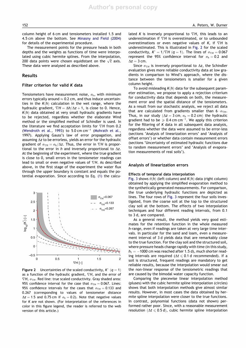
Tensiometers have measurement noise, rh, with minimumerrors typically around � 0:2 cm, and thus induce uncertain-ties in the KðhÞ calculation in the wet range, where thehydraulic gradient, rH ¼ Dh=Dzþ 1, is close to 0. Hence,KðhÞ data obtained at very small hydraulic gradients haveto be rejected, regardless whether the elaborate Windmethod or the simplified method of Schindler is used. Inthe literature we find acceptation limits for rH from 0.2(Wendroth et al., 1993) to 5:0 cm cmÿ1 (Mohrath et al.,1997). Applying Gauss’s law of error propagation, andassuming Dz to be errorless, yields an error for the hydraulicgradient of rrH ¼ rh=Dz. Thus, the error in rH is propor-tional to the error in h and inversely proportional to Dz.At the beginning of the experiment, where the true gradientis close to 0, small errors in the tensiometer readings canlead to small or even negative values of rH. As describedabove, in the first stage of the experiment the water fluxthrough the upper boundary is constant and equals the po-tential evaporation. Since according to Eq. (1) the calcu-

lated K is inversely proportional to rH, this leads to anunderestimation if rH is overestimated, or to unboundedoverestimations or even negative values of K, if rH isunderestimated. This is illustrated in Fig. 2 for the scaledconductivity, K� ¼ 1=rH ðq ¼ 1Þ. The lines of rrH ¼ 0:067represent the 95% confidence interval for rh ¼ 0:2 andDz ¼ 3 cm.

Since rrH is inversely proportional to Dz, the Schindlerevaluation gives more reliable conductivity data at low gra-dients in comparison to Wind’s approach, where the dis-tance between the tensiometers is smaller for a givencolumn height.

To avoid misleading KðhÞ data for the subsequent param-eter estimation, we propose to apply a rejection criteriumfor conductivity data that depends on both, the measure-ment error and the spatial distance of the tensiometers.As a result from our stochastic analysis, we reject all datathat are calculated from gradients smaller than 6 � rrH.Thus, in our study ðDz ¼ 3 cm; rh ¼ 0:2 cmÞ the hydraulicgradient had to be P 0:4 cm cmÿ1. We apply this criterionfor the filtering of K data in all subsequent data analysis,regardless whether the data were assumed to be error-less(sections ‘Analysis of linearization errors’ and ‘Analysis ofoffset errors’) or whether data contain measurement errors(sections ‘Uncertainty of estimated hydraulic functions dueto random measurement errors’ and ‘Analysis of evapora-tion measurements of real soils’).

Analysis of linearization errors

Effects of temporal data interpolation

Fig. 3 shows hðhÞ (left column) and KðhÞ data (right column)obtained by applying the simplified evaporation method tothe synthetically generated measurements. For comparison,the true underlying hydraulic functions are depicted aslines. The four rows of Fig. 3 represent the four soils inves-tigated, from the coarse soil at the top to the structuredclay soil at the bottom. The effects of two interpolationtechniques and four different reading intervals, from 0.1to 3 d, are compared.

As a general result, the method yields very good esti-mates for the retention function in the whole measuredh-range, even if readings are taken at very large time inter-vals. In particular for the sand and loam, even a measure-ment interval of 3 d yields data that are remarkably closeto the true function. For the clay soil and the structured soil,where pressure heads change rapidly with time (in this study,h1 ¼ ÿ1000 cm was reached after 1.5 d), much shorter read-ing intervals are required (Dt 6 0:1 d recommended). If asoil is structured, frequent readings are mandatory to getreliable results, because the interpolation would smear outthe non-linear response of the tensiometric readings thatare caused by the bimodal water capacity function.

Comparing the piecewise linear interpolation method(pluses) with the cubic hermite spline interpolation (circles)shows that both interpolation methods give almost similarresults. However, in most cases the data obtained by her-mite spline interpolation were closer to the true functions.In contrast, polynomial functions (data not shown) per-formed rather poor. Since, with a reasonable measurementresolution ðDt 6 0:5 dÞ, cubic hermite spline interpolation

Figure 2 Uncertainties of the scaled conductivity, K� ðq ¼ 1Þas a function of the hydraulic gradient, rH, and the error of

rH, rrH. Red line: true scaled conductivity. Gray shaded area:

95% confidence interval for the case that rrH ¼ 0:067. Lines:

95% confidence intervals for the cases that rrH ¼ 0:133 and

0.267 (corresponding to values of tensiometer distance

Dz ¼ 1:5 and 0.75 cm if rh ¼ 0:2). Note that negative values

for K are not shown. (For interpretation of the references in

color in this figure legend, the reader is referred to the web

version of this article.)



0 0.5 1 1.5 2 2.5 30

0.05

0.1

0.15

0.2

0.25

0.3

0.35

0.4

pF [–]

vo

l. w

ate

r co

nte

nt

[–]

spline 0.1dspline 1.0dspline 2.0dspline 3.0dplin 0.1dplin 1.0dplin 2.0dplin 3.0dtrue func

0 0.5 1 1.5 2 2.5 3–4

–3

–2

–1

0

1

2

3

pF [–]

log

10 (

K in

cm

d–1)


0 0.5 1 1.5 2 2.5 30

0.05

0.1

0.15

0.2

0.25

0.3

0.35

0.4

pF [–]

vo

l. w

ate

r co

nte

nt

[–]


0 0.5 1 1.5 2 2.5 3–6

–5

–4

–3

–2

–1

0

1

2

pF [–]

log

10 (

K in

cm

d–1)


0 0.5 1 1.5 2 2.5 30.3

0.32

0.34

0.36

0.38

0.4

pF [–]

vo

l. w

ate

r co

nte

nt

[–]


0 0.5 1 1.5 2 2.5 3–4

–3.5

–3

–2.5

–2

–1.5

–1

–0.5

0

pF []

log

10 (

K in

cm

d–1)


0 0.5 1 1.5 2 2.5 30.25

0.3

0.35

0.4

0.45

pF [–]

vo

l. w

ate

r co

nte

nt

[–]


0 0.5 1 1.5 2 2.5 3–5

–4

–3

–2

–1

0

1

2

3

4

pF [–]

log

10 (

K in

cm

d–1)


Figure 3 Output of the simplified evaporation method (without parameter estimation) for the four investigated soils with

different interpolation methods and time resolution in measurements. Left column: retention functions; right column: hydraulic

conductivity functions. First row: sand; second row: loam; third row: clay; fourth row: structured soil.



was in all cases slightly superior to the piecewise linearinterpolation, we always used cubic hermite splines forthe data interpolation in the subsequent analysis.

Effects of spatial linearization assumptions

Closer inspection of the data in Fig. 3 reveals that, even ifthey are obtained with sufficient temporal resolution, theyshow small but significant systematic deviations near satura-tion. This is most distinct for the sand and the structuredsoil, where the spatial linearization leads to an underestima-tion of the water contents in comparison to the true pointwater contents at the wet end of the measurement range.This systematic effect is caused by linearizing the non-linearwater content profile in the column at quasi-hydrostatic con-ditions. The error appears insignificant at a first sight, butsince the retention data are, in a second step, usually fittedwith a parametric model which in turn is used to estimatethe shape of the conductivity function, it can be greatlyamplified in this step (Durner, 1994). We will discuss thishðhÞ linearization error in the next subsection.

Towards the end of an evaporation experiment, the pres-sure head profile and the corresponding water content pro-file become non-linear (Fig. 1). This is most pronouncedclose to the evaporating surface and for coarse soils. Quiteremarkably, our analysis of the Schindler evaporation meth-od showed in no case that the spatial linearization assump-tion at this late stage of the experiment causes significanterrors (Fig. 3).

In contrast to water retention data, conductivity data(Fig. 3, right column) can be reliably determined only upto magnitudes where the soil’s unsaturated conductivity isin the same range as the applied evaporation flux, in ourcase 0:2 cm dÿ1. Therefore, the pressure range where reli-able data are available is rather restricted. As describedabove, this is a known general limitation of the evaporationmethod, and is due to the necessity of measuring a hydraulicgradient which is significantly different from zero. Given thetensiometer distance of 3.0 cm and the accuracy of tensi-ometers in our study ðr ¼ 0:2 cmÞ, a hydraulic gradient of� 0:4 must be present in the sample to get reliable esti-mates of KðhÞ. An improvement in the measurement accu-racy by one order of magnitude reduces the error in thedetermination of the hydraulic gradient also by one orderof magnitude (see above). Accordingly, this enables one tomeasure conductivities that reach one order of magnitudehigher. For the sand, we see that this would expand thepressure range in which reliable conductivity data can beobtained, only slightly. For direct determinations of con-ductivities near saturation, the evaporation method isunsuited (Minasny and Field, 2004; Wendroth et al., 1993).

The errors in the retention data are reflected and ampli-fied in the conductivity data. Large temporal interpolationintervals of the tensiometer data lead in particular for thefine textured clay soil and for the structured soil to signifi-cant and systematic deviations from the true function.Again, the problem is less pronounced for the coarser soils.

Effect of non-linear water content distribution near

saturation

As mentioned in the previous section, the water content dis-tribution with height in the soil column at the initial stage ofthe experiment can be significantly non-linear for coarse or

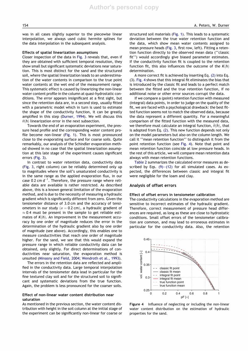
structured soil materials (Fig. 1). This leads to a systematicdeviation between the true water retention function andthe data, which show mean water contents assigned tomean pressure heads (Fig. 3, first row, left). Fitting a reten-tion function directly to the observed mean data (‘‘classicfit’’) would accordingly give biased parameter estimates.If the conductivity function fit is coupled to the retentionfunction fit, this also influences the outcome of the KðhÞdetermination.

A more correct fit is achieved by inserting Eq. (2) into Eq.(3). Fig. 4 shows that this integral fit eliminates the bias thatis introduced by the classic fit and leads to a perfect matchbetween the fitted and the true retention function, if noadditional noise or other error sources corrupt the data.

If we compare a (point) retention function with measured(integral) data points, in order to judge on the quality of thefit, we are faced with a psychological drawback: the best fit-ted function seems not to match the observed data, becausethe data represent a different quantity. For a meaningfulcomparison of the fitted function with the measured data,we therefore must calculate an integral function, �hð�hÞ, thatis adopted from Eq. (2). This new function depends not onlyon the model parameters but also on the column length. Wecall it ‘‘mean retention function’’ to distinguish it from thepoint retention function (see Fig. 4). Note that point andmean retention function coincide at low pressure heads. Inthe rest of this article, we will compare mean retention dataalways with mean retention functions.

Table 2 summarizes the calculated error measures as de-scribed by Eqs. (9)–(12) for all simulated cases. As ex-pected, the differences between classic and integral fitwere negligible for the loam and clay.

Analysis of offset errors

Effect of offset errors in tensiometer calibration

The conductivity calculations in the evaporation method aresensitive to incorrect estimates of the hydraulic gradient.Therefore, correct measurement of pressure head differ-ences are required, as long as these are close to hydrostaticconditions. Small offset errors of the tensiometer calibra-tion are common, and may lead to erroneous estimates inparticular for the conductivity data. Also, the retention

0 0.2 0.4 0.6 0.8 10.25

0.3

0.35

0.4

0.45

pF [–]

vol. w

ate

r conte

nt [–

]

classic fit pointclassic fit meanintegral fit pointintegral fit meantrue function pointtrue function mean

Figure 4 Influence of neglecting or including the non-linear

water content distribution on the estimation of hydraulic

properties for the sand.



function data close to saturation will be affected by errorsin tensiometer calibration but this effect is less pro-nounced, since it relates to the average of two measure-ments, whereas the conductivity estimates depend ondifferences.

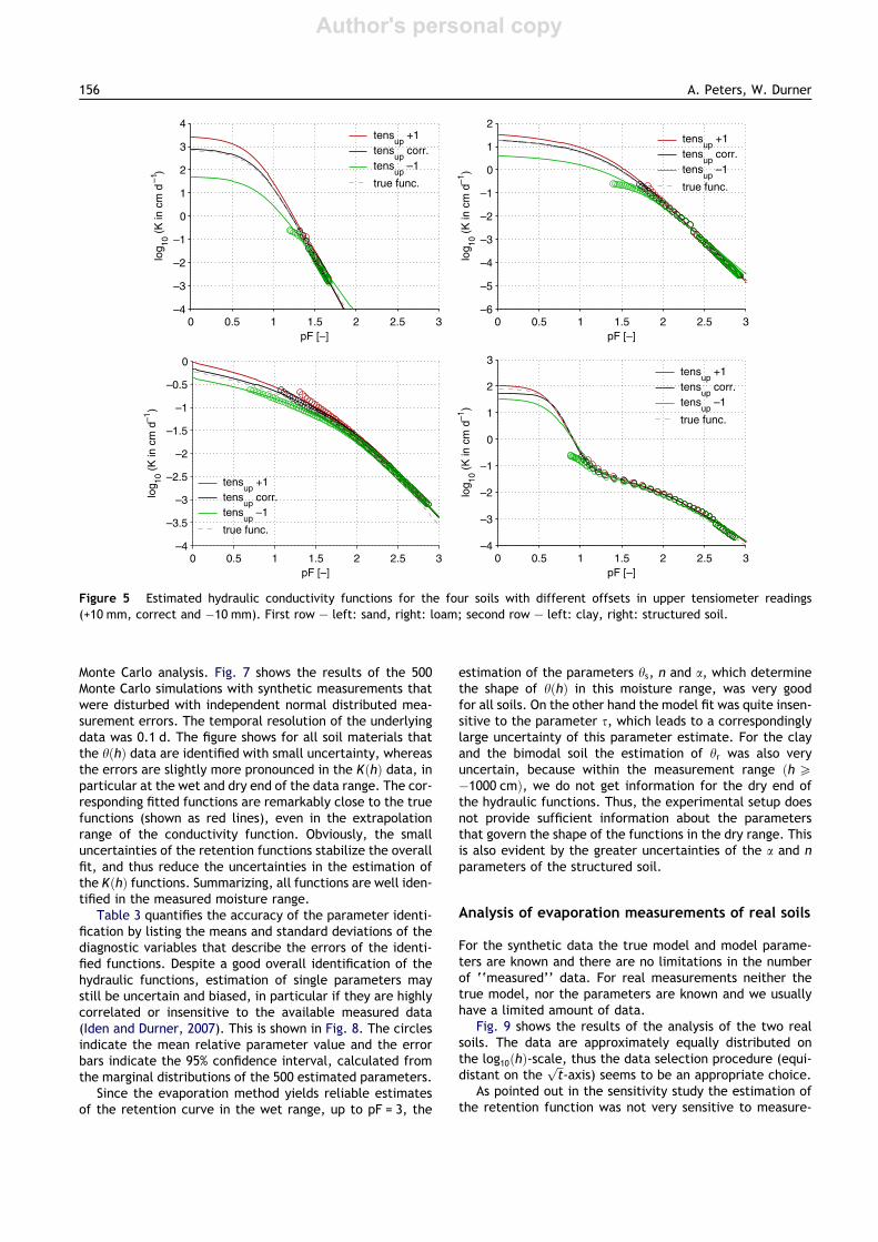
Fig. 5 shows how conductivity data and the fitted para-metric conductivity functions are affected by an offset errorof the upper tensiometer of �1 cm. An offset of ÿ1 cmleads to an underestimation of KðhÞ and vice versa. This iscaused by the corresponding under- and overestimation ofthe hydraulic gradient that is inversely proportional toKðhÞ (Eq. (1)). An overestimation of rH leads to large sys-tematic errors, whereas an underestimation basically leadsto less information in the wet range of the conductivityfunction. This is a result of the filter criterion that discardsdata at too small hydraulic gradients, whereas the overesti-mated gradients lead to biased data. The same result holdsfor corresponding offsets in the calibration of the lower ten-siometer. In the dry range, the influence of biased �hi valuesdue to calibration errors becomes negligible, due to thegreatly increased hydraulic gradients.

The estimated KðhÞ-functions show that the moderatedata errors from the underestimated hydraulic gradients

are amplified in the extrapolation range toward saturation.The errors for the sand are larger than for the finer soils.This is on one hand a result of the wide extrapolation range,where no information about the function is available, but isfurthermore caused by systematic deviations of the reten-tion function, as shown by the relatively high values ofDhmax and RMSEh (Table 2). An offset of �1 cm in the tensi-ometer calibration leads to an offset of �0:5 cm in �hi for acertain �hi. Similar to the previously discussed non-linearwater content distribution, these offset errors affect thecalculation of the water retention data particularly forcoarse sands and structured soils in the wet range. The com-bined effects of a slightly biased retention curve estimateand the biased conductivity data leads to the differencesin the estimated conductivity curve in the interpolatedrange.

Effect of errors in tensiometer position

Slight deviations in the positioning of the installed tensiom-eters are unavoidable in practice. We therefore investi-gated the consequences of placement errors of the uppertensiometer of �0:42 cm, which yielded some interestingaspects. In general, we found only small deviations betweenretention data and the true functions. The estimated reten-tion function for the sand (not shown) has some deviationsin the wet range, whereas the estimation of the retentionfunction for the clay (Fig. 6, first row) and loam (not shown)exhibit the deviations in the dry range. The deviation in thewet range of the sand may be explained in the same way asthe outcome of the offset in the tensiometer calibration. Infact, as long as the hðzÞ distribution is linear the effects ofwrong tensiometer position and wrong tensiometer calibra-tion are identical.

The deviation in the dry range is due to the very strongnon-linearity of the pressure head distribution in the secondstage of the evaporation experiment (Fig. 1). In this stagethe pressure head 0.42 cm above or below the proper uppertensiometer location may be one or two orders of magni-tude lower or higher, leading to lower or higher �hi for a cer-tain hi and thus to an over- or underestimation of theretention function in the dry range. Since the bimodal soilcombines a coarse with a fine pore system, both errorsare coupled in the bimodal soil (Fig. 6, second row).

The calculated conductivities are only slightly affectedby the offset error in tensiometer position. In the rangewhere the data pairs are not rejected due to small hydraulicgradients the errors in the conductivity prediction areacceptable for all soils, although the error is most pro-nounced in the clay soil, where the pressure head distribu-tion becomes non-linear in a very early stage of theexperiment. In the wet range (close to Ks), the deviationsappear greater, which is caused by smaller gradients in thatstage, and thus larger relative errors in the gradient, as out-lined above.

Uncertainty of estimated hydraulic functions due to

random measurement errors

We expected that noise in the measurements will increasethe uncertainty of parameter estimates, but will not inducea systematic bias in the results. This was confirmed by our

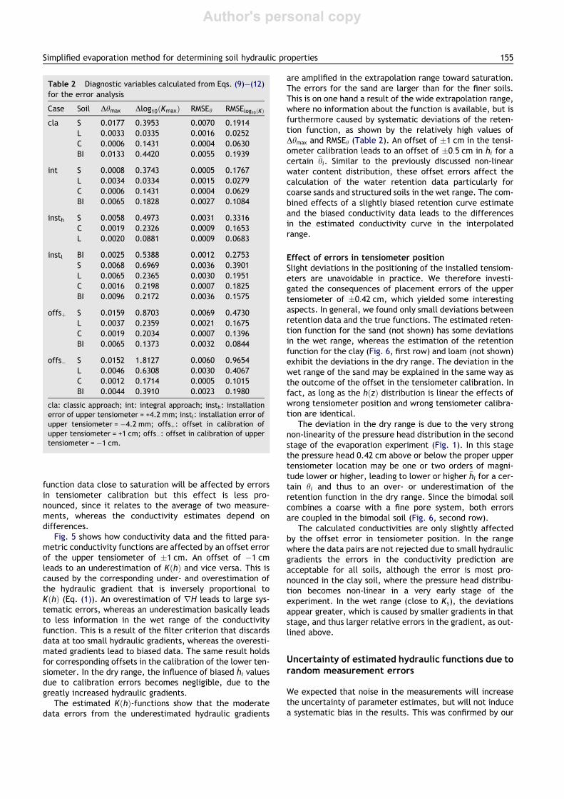
Table 2 Diagnostic variables calculated from Eqs. (9)–(12)

for the error analysis

Case Soil Dhmax Dlog10ðKmaxÞ RMSEh RMSElog10ðKÞ

cla S 0.0177 0.3953 0.0070 0.1914

L 0.0033 0.0335 0.0016 0.0252

C 0.0006 0.1431 0.0004 0.0630

BI 0.0133 0.4420 0.0055 0.1939

int S 0.0008 0.3743 0.0005 0.1767

L 0.0034 0.0334 0.0015 0.0279

C 0.0006 0.1431 0.0004 0.0629

BI 0.0065 0.1828 0.0027 0.1084

insth S 0.0058 0.4973 0.0031 0.3316

C 0.0019 0.2326 0.0009 0.1653

L 0.0020 0.0881 0.0009 0.0683

instl BI 0.0025 0.5388 0.0012 0.2753

S 0.0068 0.6969 0.0036 0.3901

L 0.0065 0.2365 0.0030 0.1951

C 0.0016 0.2198 0.0007 0.1825

BI 0.0096 0.2172 0.0036 0.1575

offsþ S 0.0159 0.8703 0.0069 0.4730

L 0.0037 0.2359 0.0021 0.1675

C 0.0019 0.2034 0.0007 0.1396

BI 0.0065 0.1373 0.0032 0.0844

offsÿ S 0.0152 1.8127 0.0060 0.9654

L 0.0046 0.6308 0.0030 0.4067

C 0.0012 0.1714 0.0005 0.1015

BI 0.0044 0.3910 0.0023 0.1980

cla: classic approach; int: integral approach; insth: installationerror of upper tensiometer = +4.2 mm; instl: installation error ofupper tensiometer = ÿ4.2 mm; offsþ: offset in calibration ofupper tensiometer = +1 cm; offsÿ: offset in calibration of uppertensiometer = ÿ1 cm.



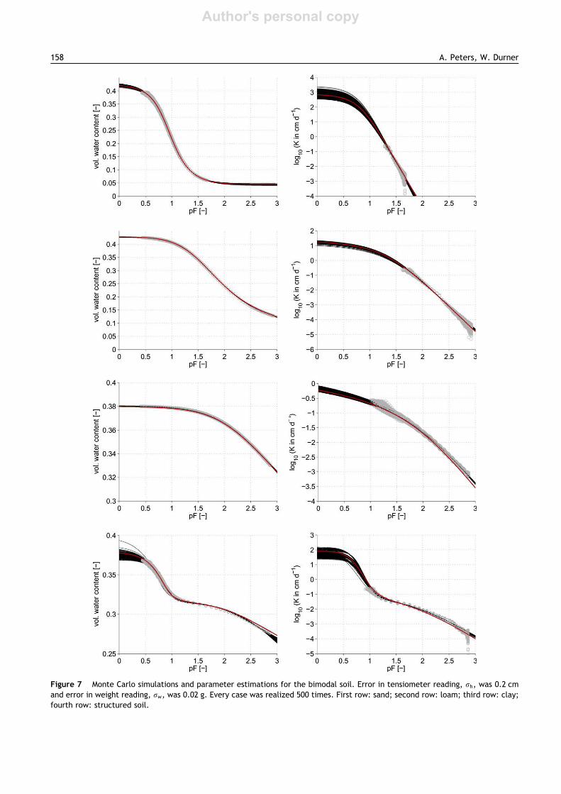
Monte Carlo analysis. Fig. 7 shows the results of the 500Monte Carlo simulations with synthetic measurements thatwere disturbed with independent normal distributed mea-surement errors. The temporal resolution of the underlyingdata was 0.1 d. The figure shows for all soil materials thatthe hðhÞ data are identified with small uncertainty, whereasthe errors are slightly more pronounced in the KðhÞ data, inparticular at the wet and dry end of the data range. The cor-responding fitted functions are remarkably close to the truefunctions (shown as red lines), even in the extrapolationrange of the conductivity function. Obviously, the smalluncertainties of the retention functions stabilize the overallfit, and thus reduce the uncertainties in the estimation ofthe KðhÞ functions. Summarizing, all functions are well iden-tified in the measured moisture range.

Table 3 quantifies the accuracy of the parameter identi-fication by listing the means and standard deviations of thediagnostic variables that describe the errors of the identi-fied functions. Despite a good overall identification of thehydraulic functions, estimation of single parameters maystill be uncertain and biased, in particular if they are highlycorrelated or insensitive to the available measured data(Iden and Durner, 2007). This is shown in Fig. 8. The circlesindicate the mean relative parameter value and the errorbars indicate the 95% confidence interval, calculated fromthe marginal distributions of the 500 estimated parameters.

Since the evaporation method yields reliable estimatesof the retention curve in the wet range, up to pF = 3, the

estimation of the parameters hs, n and a, which determinethe shape of hðhÞ in this moisture range, was very goodfor all soils. On the other hand the model fit was quite insen-sitive to the parameter s, which leads to a correspondinglylarge uncertainty of this parameter estimate. For the clayand the bimodal soil the estimation of hr was also veryuncertain, because within the measurement range ðh P

ÿ1000 cmÞ, we do not get information for the dry end ofthe hydraulic functions. Thus, the experimental setup doesnot provide sufficient information about the parametersthat govern the shape of the functions in the dry range. Thisis also evident by the greater uncertainties of the a and n

parameters of the structured soil.

Analysis of evaporation measurements of real soils

For the synthetic data the true model and model parame-ters are known and there are no limitations in the numberof ‘‘measured’’ data. For real measurements neither thetrue model, nor the parameters are known and we usuallyhave a limited amount of data.

Fig. 9 shows the results of the analysis of the two realsoils. The data are approximately equally distributed onthe log10ðhÞ-scale, thus the data selection procedure (equi-distant on the

ffiffit

p-axis) seems to be an appropriate choice.

As pointed out in the sensitivity study the estimation ofthe retention function was not very sensitive to measure-

0 0.5 1 1.5 2 2.5 3–4

–3

–2

–1

0

1

2

3

4

pF [–]

log

10 (

K in c

m d

–1 )

0 0.5 1 1.5 2 2.5 3–6

–5

–4

–3

–2

–1

0

1

2

pF [–]

log

10 (

K in c

m d

–1)

tensup

+1

tensup

corr.

tensup

–1

true func.

0 0.5 1 1.5 2 2.5 3–4

–3.5

–3

–2.5

–2

–1.5

–1

–0.5

0

pF [–]

log

10 (

K in

cm

d–

1)

tensup

+1

tensup

corr.

tensup

–1

true func.

0 0.5 1 1.5 2 2.5 3–4

–3

–2

–1

0

1

2

3

pF [–]

log

10 (

K in c

m d

–1)

tensup

+1

tensup

corr.

tensup

–1

true func.

tensup

+1

tensup

corr.

tensup

–1

true func.

Figure 5 Estimated hydraulic conductivity functions for the four soils with different offsets in upper tensiometer readings

(+10 mm, correct and ÿ10 mm). First row – left: sand, right: loam; second row – left: clay, right: structured soil.



ment errors. This result can also be seen in the evaluation ofthe two soils, where the retention data are rather smoothand well described by the unimodal van Genuchten func-tion. However, the small but systematic misfit of the sandyloam data (Fig. 9, top) indicates that the van Genuchtenmodel cannot perfectly describe this soil.

Again, the more crucial part was the estimation of thehydraulic conductivity function. Due to low gradients inthe beginning of the experiment, conductivity data for thesandy loam where only available for pressure heads<ÿ100 cm. For the clay, the gradient increased already atlow pressure heads and thus conductivity data were avail-able at higher pressure heads (<ÿ60 cm). The conductivitydata of the sandy loam could be well described with thevan Genuchten/Mualem model, whereas the conductivitydata of the clay show deviations in the wet and in the dryrange, indicating either a bias in the measurements, i.e.an underestimation of the hydraulic gradient in the wetrange (see above) or a wrong model assumption. The latteris observed frequently in the dry range of the conductivityfunction, where the capillary bundle models such as theone of Mualem (1976) do not well describe the flow behav-ior. One possible explanation for this is the negligence ofthe film flow leading to an underestimation of the conduc-tivity in the dry range (Tuller and Or, 2001).

The independently measured saturated hydraulic con-ductivity, Ks, was � 1300 cm dÿ1 for the sandy loam, thatis about two orders of magnitude higher than estimated.

This reflects the uncertainty of the parametric extrapola-tion of KðhÞ in the wet range. For the clay no independentKs measurement was available.

Although the model fits are not perfect the largest devi-ation on the KðhÞ-curve is half an order of magnitude, andthus in most applications still justifiable. Nevertheless themeasurement results show that the model structure (espe-cially the KðhÞ-model) needs to be improved to better de-scribe the natural soils.

Discussion

Quite remarkably, our analysis of the Schindler evaporationmethod showed in no case that the spatial linearizationassumption at the late stage of the experiment causes sig-nificant errors (Fig. 3). In contrast, the non-linearity ofthe retention function turned out to yield small but system-atic errors at the beginning of the experiment. These arenon-negligible for coarse soils or soils with a structural poresystem, in particular, if the retention data are used in aparameter estimation procedure to derive simultaneouslythe coupled retention and conductivity function. We couldshow that this error can be fully avoided by using the inte-gral approach of Peters and Durner (2006) in the parameterestimation. In the early phase of evaporation experiments,the most severe handicap is the uncertainty in determiningthe hydraulic gradient. Since this uncertainty is inversely

0 0.5 1 1.5 2 2.5 30.3

0.32

0.34

0.36

0.38

0.4

pF [–]

vol. w

ate

r conte

nt [–

]

tensup

high

tensup

corr.

tensup

low

true func.

0 0.5 1 1.5 2 2.5 3–4

–3.5

–3

–2.5

–2

–1.5

–1

–0.5

0

pF [–]

log

10 (

K in

cm

d–1 )

tensup

high

tensup

corr.

tensup

low

true func.

0 0.5 1 1.5 2 2.5 30.25

0.3

0.35

0.4

pF [–]

vol. w

ate

r conte

nt [–

]

tensup

high

tensup

corr.

tensup

low

true func.

0 0.5 1 1.5 2 2.5 3–4

–3

–2

–1

0

1

2

3

pF [–]

log

10 (

K in c

m d

–1 )

tensup

high

tensup

corr.

tensup

low

true func.

Figure 6 Estimated hydraulic properties for the clay (first row) and the structured soil (second row) with different offsets in upper

tensiometer installation (4.2 mm high, correct and 4.2 mm low). Left column: retention functions; right column: hydraulic

conductivity functions.



Figure 7 Monte Carlo simulations and parameter estimations for the bimodal soil. Error in tensiometer reading, rh, was 0.2 cm

and error in weight reading, rw, was 0.02 g. Every case was realized 500 times. First row: sand; second row: loam; third row: clay;

fourth row: structured soil.



proportional to the distance between tensiometers, and theWind evaporation method requires smaller distances be-tween tensiometers for a certain column height, we con-clude that the Schindler evaporation method is superior toWind’s method in the wet moisture range. By basing therejection criterion for KðhÞ data in the wet range on the er-ror in the hydraulic gradient we introduced an applicable fil-ter for reliable data ranges.

Errors in the calibration of tensiometers lead to someinteresting effects. A negative offset of the upper tensiom-eter or a positive offset of the lower tensiometer will causea significant underestimation of the conductivity close tosaturation. The opposite offsets, however, do not cause abias but only lead to a lack of information in that pressurehead range, due to the rejection criterion based on the min-imum magnitude of the hydraulic gradient. An offset in thetensiometer installation has principally the same effect asthe offset in the calibration for the wet range. Since theinstallation error in properly performed experiments is onlyin the range of millimeters, whereas an offset in tensiome-ter calibration can easily reach one or more centimeters,the installation error has much less severe impacts in thewet moisture range. In the dry range, we found that aninstallation error can also cause systematic errors in bothhydraulic functions due to the non-linearity of the pressurehead distribution.

The results for the linearization errors in time indicatethat the measuring interval for the tensiometer readingsshould be small ð6 0:1 dÞ for fine textured materials. Thissuggests that tensiometer readings should be recorded byautomatic data logging. Sample weights, on the other hand,can be recorded manually at very large time intervals, be-cause the weight change during the first stage of evapora-tion is linear and the second stage of evaporation is not

Table 3 Distribution of diagnostic variables calculated

from Eqs. (9)–(12) for the Monte Carlo simulations

Case Soil Dhmax Dlog10ðKmaxÞ RMSEh RMSElog10ðKÞ

l S 0.0026 0.4089 0.0014 0.2014

L 0.0034 0.0433 0.0015 0.0318

C 0.0006 0.1479 0.0004 0.0659

BI 0.0065 0.2357 0.0026 0.1282

r S 0.0012 0.2197 0.0006 0.0965

L 0.0002 0.0218 0.0001 0.0155

C 0.0001 0.0162 0.0000 0.0093

BI 0.0016 0.0945 0.0007 0.0412

l is the arithmetic mean and r is the standard deviation of thediagnostic variable.

0

0.5

1

1.5

2

rel. p

ara

me

ter

valu

e [

–]

α n θr

θs τ K

s

0

0.5

1

1.5

2

rel. p

ara

me

ter

valu

e [

–]

α n θr

θs τ K

s

0

0.5

1

1.5

2

rel. p

ara

me

ter

va

lue [

–]

α n θr

θs τ K

s

o.o

.R.

0

0.5

1

1.5

2

rel. p

ara

me

ter

va

lue [

–]

α1

n1

θr

θs τ K

sα

2n

2w

2

Figure 8 Relative estimated parameter values and their 95% confidence interval. Gray dashed line: true relative parameter value;

circles: mean of estimated relative parameter; bars: 95% confidence interval of estimated relative parameter distribution. (A) Sand;

(B) loam; (C) clay; (D) bimodal soil.



reached for these materials (Kutilek and Nielsen, 1994). Incontrast to that, coarse materials do reach the second stageof evaporation, and thus the sample weights decrease non-linear with time. However, even for a coarse sand a mea-surement resolution of 2 d was sufficient. Thus, the lineari-zation errors with respect to time are negligible if a properselection of time intervals and interpolation of the mea-surements is chosen.

Our final analysis of noisy measurement data that werefitted with parametric models showed that most of theretention curve and conductivity curve parameters can beestimated with small uncertainties. Even if finer materialsare investigated, where the dry end of the retention func-tion is not reached in the course of the experiment, onlythe estimation of hr becomes uncertain. Due to lack of con-ductivity data close to saturation, the parameters that de-scribe the KðhÞ function can only be estimated by trustingthe coupling of the retention and conductivity model. Inour investigated cases, the small uncertainties in the reten-tion function lead to relatively small errors in the fits of theconductivity function.

We like to stress at this point that in all cases of our anal-ysis, we assumed that the underlying retention and conduc-tivity models were exactly known and thus the coupling ofboth functions indeed contributed to a reliable parameterestimation. For real soils, this assumption will never be per-fectly met, and the analysis of two real data sets confirmedthat in particular the extrapolation of estimated conductiv-ity curves toward saturation must be interpreted with care.

Conclusions

A comprehensive error analysis of the simplified evapora-tion method showed that it is a fast, accurate and reliablemethod to determine soil hydraulic properties in the mea-sured pressure head range. The method relies on four dif-ferent linearization assumptions in time and space. Byusing the integral approach for parameter estimation weeliminated one of these linearization errors, which im-proves the estimation of hydraulic properties of coarsesoils or soils with a secondary pore system. The remainingthree linearization assumptions are of minor effect for theestimation of the retention function for soils of any tex-ture, if the measurement interval for the pressure headsis reasonable short and a suitable data interpolation, suchas cubic hermite splines, is used. The determination ofhydraulic conductivity data and the subsequent estimationof the conductivity function was also very reliable in thedry range. However, with the evaporation method we donot get data for the KðhÞ-function in the wet range, sothat at least an additional measurement of Ks should beprovided. Also, the shape of the conductivity function inthe wet range must be interpreted with care. To improvethe characterization of the conductivity function near sat-uration, alternative methods, such as multi-step outflowmethods in combination with free-form parameter estima-tion will be required.

In addition to the investigation of the linearization er-rors, we investigated error sources introduced by offsets

0 0.5 1 1.5 2 2.5 30

0.05

0.1

0.15

0.2

0.25

0.3

0.35

0.4

pF [–]

vol. w

ate

r conte

nt [–

]

0 0.5 1 1.5 2 2.5 3–4

–3

–2

–1

0

1

2

pF [–]

log

10 (

K in c

m d

–1 )

0 0.5 1 1.5 2 2.5 30.2

0.25

0.3

0.35

0.4

0.45

0.5

0.55

pF [–]

vol. w

ate

r conte

nt [–

]

0 0.5 1 1.5 2 2.5 3–5

–4

–3

–2

–1

0

1

2

3

pF [–]

log

10 (

K in c

m d

–1 )

Figure 9 Output of the simplified evaporation method and estimated hydraulic properties for the sandy loam (first row) and the

clay (second row).



in the tensiometer calibrations, offsets in tensiometerinstallation or random error in the measurement readings.Altogether, the errors in the estimated data were remark-ably small, in particular for the retention curve. Tensiome-ter calibration errors lead in coarse materials to erroneousestimations of the hydraulic functions in the wet range.Especially, the estimation of the conductivity function closeto saturation becomes severely biased. Errors due to wrongtensiometer position are less severe. Thus, the most crucialpart of applying the method is the use of reliable tensio-meters.

Acknowledgements

We thank Budiman Minasny (University of Sydney) for pro-viding data of evaporation experiments for two soils, andGeorg von Unold (UMS GmbH – Umweltanalytische Mess-Systeme) and Sascha Iden for fruitful discussions.

References

Bertuzzi,P.,Mohrath,D.,Bruckler,L.,Gaudu,J.C.,Bourlet,M.,1999.Wind’s evaporation method: experimental equipment anderror analysis. In: van Genuchten, M.T., Leij, F.J., Wu, L. (Eds.),ProceedingsoftheInternationalWorkshoponCharacterizationandMeasurement of the Hydraulic Properties of Unsaturated PorousMedia, University of California, Riverside, CA, pp. 323–328.

Bitterlich, S., Durner, W., Iden, S.C., Knabner, P., 2004. Inverseestimation of the unsaturated soil hydraulic properties fromcolumn outflow experiments using free-form parameterizations.Vadose Zone J. 3, 971–981.

Boels, D., Gils, J.B.H.M.v., Veerman, G.J., Wit, K.E., 1978. Theoryand system of automatic determination of soil moisture char-acteristics and unsaturated hydraulic conductivities. Soil Sci.126 (4), 191–199.

Bouma, J., Belmans, C., Dekker, L.W., Jeurissen, W.J.M., 1983.Assessing the suitability of soils with macropores for subsurfaceliquid waste disposal. J. Environ. Qual. 12 (3), 305–311.

Coppola, A., 2000. Unimodal and bimodal description of hydraulicproperties for aggregated soils. Soil Sci. Soc. Am. 64, 1252–1262.

Dane, J., Hopmans, J., 2002. Water retention and storage/labora-tory. In: Dane, J., Topp, G. (Eds.), Methods of Soil Analysis. Part4: Physical Methods. SSSA Book Series: 5. Soil Science Society ofAmerica Inc., pp. 675–720.

Dirksen, C., 1991. Unsaturated hydraulic conductivity. In: Smith,K.A., Mullins, C.E., Dekker, M. (Eds.), Soil Analysis PhysicalMethods. New York, pp. 209–270.

Duan, Q., Sorooshian, S., Gupta, V., 1992. Effective and efficientglobal optimization for conceptual rainfall-runoff models. WaterResour. Res. 28, 1015–1031.

Durner, W., 1994. Hydraulic conductivity estimation for soils withheterogeneous pore structure. Water Resour. Res. 30, 211–223.

Durner, W., Lipsius, K., 2005. Chapter 75: determining soil hydraulicproperties. In: Anderson,M.,McDonnell, J.J. (Eds.), Encyclopediaof Hydrological Sciences. John Wiley &Sons Ltd., pp. 1021–1144.

Durner, W., Schultze, B., Zurmuhl, T., 1999. State-of-the-art ininverse modeling of inflow/outflow experiments. In: vanGenuchten, M.T., Leij, F.J., Wu, L. (Eds.), Proceedings of theInternational Workshop on Characterization and Measurement ofthe Hydraulic Properties of Unsaturated PorousMedia, Universityof California, Riverside, CA, pp. 661–681.

Fritsch, F.N., Carlson, R.E., 1980. Monotone piecewise cubicinterpolation. SIAM J. Numer. Anal. 17, 238–246.

Halbertsma, J., Veerman, G., 1994. A new calculation procedureand simple set-up for the evaporation method to determine soilhydraulic functions. Tech. Rep., DLO Winand Staring Centre,Wageningen, The Netherlands.

Hoffmann-Riem, H., van Genuchten, M.T., Fluhler, H., 1999.General model for the hydraulic conductivity of unsaturatedsoils. In: van Genuchten, M.T., Leij, F.J., Wu, L. (Eds.), Pro-ceedings of the International Workshop on Characterization andMeasurement of the Hydraulic Properties of Unsaturated PorousMedia, University of California, Riverside, CA, pp. 31–42.

Hopmans, J.W., Simunek, J., Romano, N., Durner, W., 2002.Simultaneous determination of water transmission and retentionproperties. Inverse methods. In: Dane, J., Topp, G. (Eds.),Methods of Soil Analysis. Part 4: Physical Methods. Soil ScienceSociety of America Inc., pp. 963–1004.

Iden, S., Durner, W., 2007. Free-form estimation of the unsaturatedsoil hydraulic properties by inverse modeling using globaloptimization. Water Resour. Res. 43, w07451. doi:10.1029/2006WR005845.

Kutilek, M., Nielsen, D., 1994. Soil Hydrology. Catena VerlagGeoEcology Publications, Cremlingen-Destedt, pp. 188–189.

Lambot, S., Javaux, M., Hupet, F., Vanclooster, M., 2002. A globalmultilevel coordinate search procedure for estimating theunsaturated soil hydraulic properties. Water Resour. Res. 38(11), 1224. doi:10.1029/2001WR001224.

Mallants, D., Tseng, P.H., Toride, N., Timmerman, A., Feyen, J.,1997. Evaluation of multimodal hydraulic functions in charac-terizing a heterogeneous field soil. J. Hydrol. 195, 172–199.

Marquardt, D., 1963. An algorithm for least-squares estimation ofnonlinear parameters. SIAM J. Appl. Math. 11, 431–441.

Minasny, B., Field, D., 2004. Estimating soil hydraulic propertiesand their uncertainty: the use of stochastic simulation in theinverse modelling of the evaporation experiment. Geoderma126, 277–290.

Mohrath, D., Bruckler, L., Bertuzzi, P., Gaudu, J.C., Bourlet, M.,1997. Error analysis of an evaporation method for determininghydrodynamic properties in unsaturated soil. Soil Sci. Soc. Am.J. 61, 725–735.

Mualem, Y., 1976. A new model for predicting the hydraulicconductivity of unsaturated porous media. Water Resour. Res.12 (3), 513–521.

Othmer, H., Diekkruger, B., Kutilek, M., 1991. Bimodal porosity andunsaturated hydraulic conductivity. Soil Sci. 152 (3), 139–149.

Peters, A., Durner, W., 2006. Improved estimation of soil waterretention characteristics from hydrostatic column experiments.Water Resour. Res. 42, w11401. doi:10.1029/2006WR004952.

Plagge, R., Haeupl, P., Renger, M., 1999. Transient effects on thehydraulic properties of porous media. In: van Genuchten, M.T.,Leij, F.J., Wu, L. (Eds.), Proceedings of the InternationalWorkshop on Characterization and Measurement of the Hydrau-lic Properties of Unsaturated Porous Media, University ofCalifornia, Riverside, CA, pp. 905–912.

Priesack, E., Durner, W., 2006. Closed form expression for themulti-modal unsaturated conductivity function. Vadose Zone J.5, 121–124.

Romano, N., Santini, A., 1999. Determining soil hydraulic functionsfrom evaporation experiments by a parameter estimationapproach: experimental verifications and numerical studies.Water Resour. Res. 35, 3343–3359.

Schaap, M.G., Leij, F.J., 2000. Improved prediction of unsaturatedhydraulic conductivity with the Mualem–van Genuchten model.Soil Sci. Soc. Am. J. 64, 843–851.

Schaap, M.G., Leij, F.J., van Genuchten, M.T., 1998. Neuralnetwork analysis for hierarchical prediction of soil hydraulicproperties. Soil Sci. Soc. Am. J. 62, 847–855.

Schindler, U., 1980. Ein Schnellverfahren zur Messung der Wasser-leitfahigkeit im teilgesattigten Boden an Stechzylinderproben.Arch. Acker-u. Pflanzenbau u. Bodenkd. Berlin 24, 1–7.



Schindler, U., Muller, L., 2006. Simplifying the evaporation methodfor quantifying soil hydraulic properties. J. Plant Nutr. Soil Sci.169, 623–629. doi:10.1002/jpln.200521895.

Simunek, J., Hopmans, J., 2002. Parameter optimization andnonlinear fitting. In: Dane, J.H., Topp, G.C. (Eds.), Methods ofSoil Analysis. Part 4: Physical Methods, vol. 5. Soil ScienceSociety of America Book, Madison, WI, pp. 139–157.

Simunek, J., Wendroth, O., van Genuchten, M.T., 1998a.Parameter estimation analysis of the evaporation methodfor determining soil hydraulic properties. Soil Sci. Soc. Am. J.62, 894–905.

Simunek, L., Huang, K., Sejna, M., van Genuchten, M.T., 1998b.The hydrus-1d software package for simulating the one-dimen-sional movement of water, heat and multiple solutes in variably-saturated media, version 2.02.

Spohrer, K., Herrmann, L., Ingwersen, J., Stahr, K., 2005. Appli-cability of uni- and bimodal retention functions for water flowmodeling in a tropical acrisol. Vadose Zone J. 5, 48–58.

Tamari, S., Bruckler, L., Halbertsma, J., Chadoeuf, J., 1993. Asimple method for determining soil hydraulic properties in thelaboratory. Soil Sci. Soc. Am. J. 57, 642–651.

Tuller, M., Or, D., 2001. Hydraulic conductivity of variablysaturated porous media: film and corner flow in angular porespace. Water Resour. Res. 31 (5), 1257–1276.

van Genuchten, M.T., 1980. A closed-form equation for predictingthe hydraulic conductivity of unsaturated soils. Soil Sci. Soc.Am. J. 44, 892–898.

van Genuchten, M.T., Leij, F.J., Wu, L., 1999. Characterization andmeasurement of the hydraulic properties of unsaturated porousmedia. In: van Genuchten, M.T., Leij, F.J., Wu, L. (Eds.),Proceedings of the International Workshop on Characterizationand Measurement of the Hydraulic Properties of UnsaturatedPorous Media, University of California, Riverside, CA, pp. 1–12.

Wendroth, O., Ehlers, W., Hopmans, J.W., Klage, H., Halbertsma,J., Wosten, J.H.M., 1993. Reevaluation of the evaporationmethod for determining hydraulic functions in unsaturated soils.Soil Sci. Soc. Am. J. 57, 1436–1443.

Wind, G.P., 1968. Capillary conductivity data estimated by a simplemethod. In: Rijtema, P.E., Wassink, H. (Eds.), Water in theUnsaturated Zone, vol. 1. Proceedings of the WageningenSymposium, 19–23 June 1966. Int. Assoc. Sci. Hydrol. Publ.(IASH), Gentbrugge, The Netherlands and UNESCO, Paris.


simpliﬁed evaporation method for determining soil ... · pdf fileauthor's personal copy...

Documents