simplified methods for electronic structure calculations jorge kohanoff queen’s university belfast...

SIMPLIFIED METHODS FOR ELECTRONIC STRUCTURE

CALCULATIONS

Jorge KohanoffQueen’s University Belfast

United Kingdom

[email protected]

CCMS Summer InstituteLLNL 23 July 2012

QUEEN’S UNIVERSITY BELFASTNORTHERN IRELAND, UK

THE PROBLEM: NUCLEI AND ELECTRONS INTERACTING VIA COULOMB FORCES

Hamiltonian of the universe

neeeennn VVTVTH

2

1

2 1

2 I

P

I In MT

P

I

P

IJ JI

JInn

ZZeV

1

2

||2 RR

N

iie m

T1

22

2

N

i

N

ij jiee

eV

1

2

||

1

2 rr

N

i

P

I Ii

Ine

ZeV

1 1

2

||2 Rr

);,();,(

tHt

ti Rr

Rr

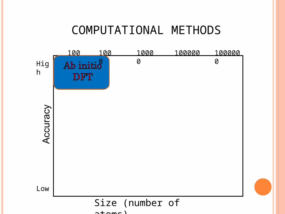
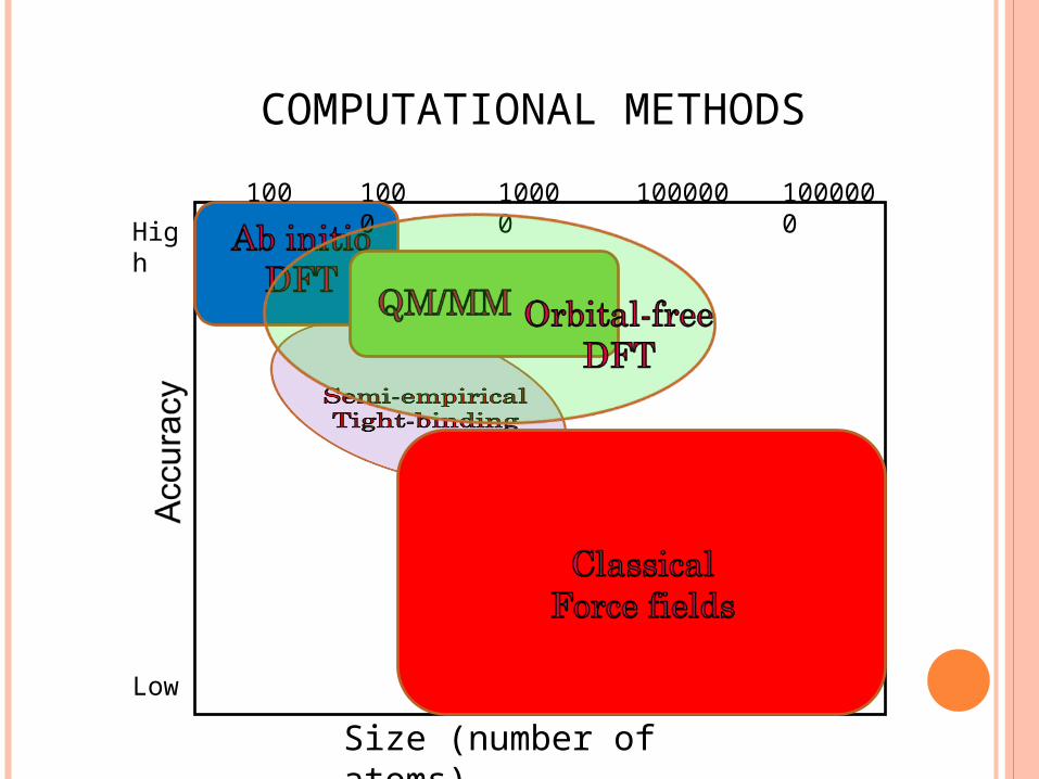
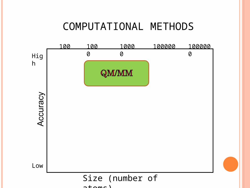
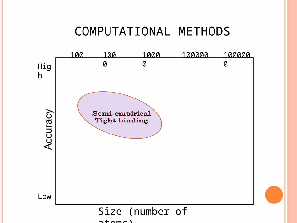
COMPUTATIONAL METHODS

Size (number of atoms)

1000

10000

1000000

100000100

High

Low

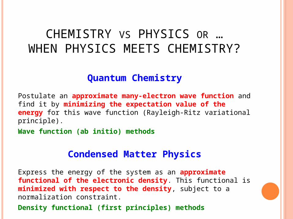
Quantum Chemistry

Postulate an approximate many-electron wave function and find it by minimizing the expectation value of the energy for this wave function (Rayleigh-Ritz variational principle).

Wave function (ab initio) methods

Condensed Matter Physics

Express the energy of the system as an approximate functional of the electronic density. This functional is minimized with respect to the density, subject to a normalization constraint.

Density functional (first principles) methods

CHEMISTRY VS PHYSICS OR …WHEN PHYSICS MEETS CHEMISTRY?

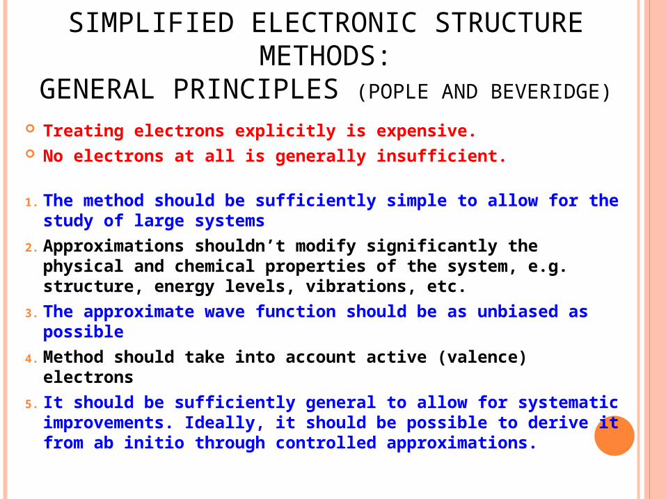
Treating electrons explicitly is expensive. No electrons at all is generally insufficient.

1. The method should be sufficiently simple to allow for the study of large systems

2. Approximations shouldn’t modify significantly the physical and chemical properties of the system, e.g. structure, energy levels, vibrations, etc.

3. The approximate wave function should be as unbiased as possible

4. Method should take into account active (valence) electrons

5. It should be sufficiently general to allow for systematic improvements. Ideally, it should be possible to derive it from ab initio through controlled approximations.

SIMPLIFIED ELECTRONIC STRUCTURE METHODS:

GENERAL PRINCIPLES (POPLE AND BEVERIDGE)



1000

10000

1000000

100000100

High

Low

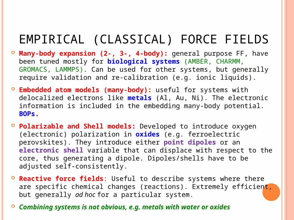
Many-body expansion (2-, 3-, 4-body): general purpose FF, have been tuned mostly for biological systems (AMBER, CHARMM, GROMACS, LAMMPS). Can be used for other systems, but generally require validation and re-calibration (e.g. ionic liquids).

Embedded atom models (many-body): useful for systems with delocalized electrons like metals (Al, Au, Ni). The electronic information is included in the embedding many-body potential. BOPs.

Polarizable and Shell models: Developed to introduce oxygen (electronic) polarization in oxides (e.g. ferroelectric perovskites). They introduce either point dipoles or an electronic shell variable that can displace with respect to the core, thus generating a dipole. Dipoles/shells have to be adjusted self-consistently.

Reactive force fields: Useful to describe systems where there are specific chemical changes (reactions). Extremely efficient, but generally ad hoc for a particular system.

Combining systems is not obvious, e.g. metals with water or oxides

EMPIRICAL (CLASSICAL) FORCE FIELDS



1000

10000

1000000

100000100

High

Low

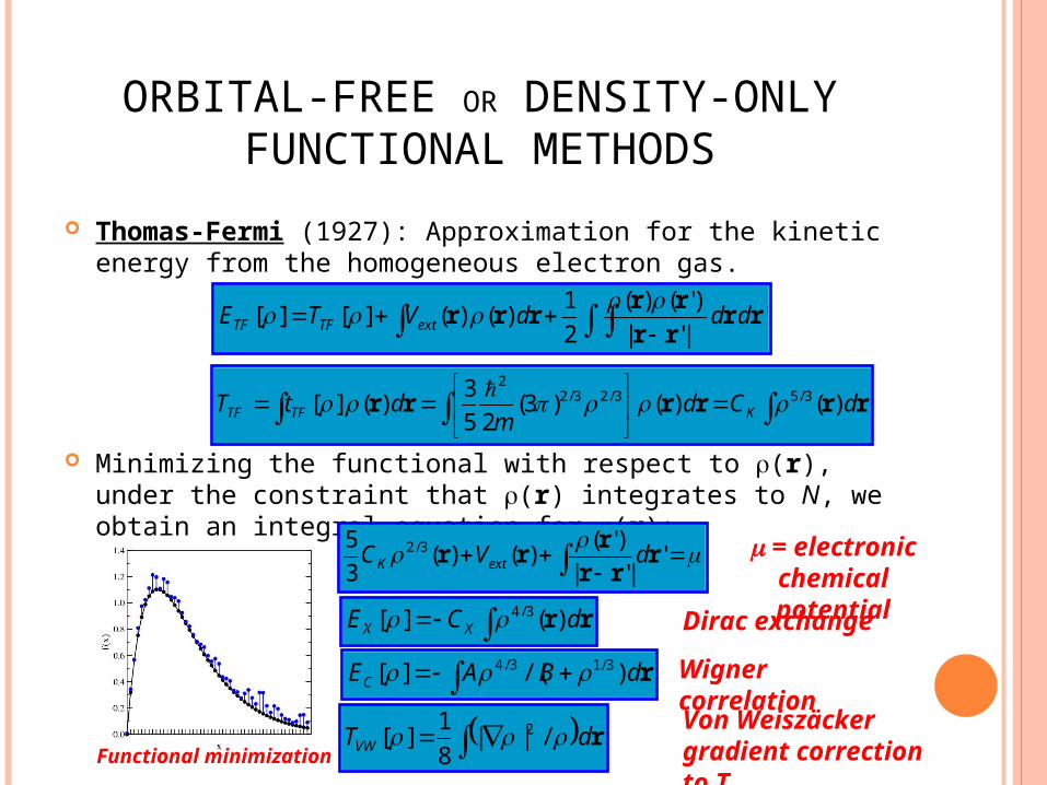
Functional minimization

Thomas-Fermi (1927): Approximation for the kinetic energy from the homogeneous electron gas.

Minimizing the functional with respect to (r), under the constraint that (r) integrates to N, we obtain an integral equation for (r):

'

|'|

)'()(

2

1)()(][][ rr

rr

rrrrr dddVTE extTFTF

'|'|

)'()()(

3

5 3/2 rrr

rrr dVC extK

= electronic chemical potential

rr dCE XX )(][ 3/4

rdBAEC )/(][ 3/13/4

rdTVW /||8

1][ 2

Dirac exchange

Wigner correlation

Von Weiszäcker gradient correction to T

rrrrrr dCd

mdtT KTFTF )()()3(

25

3)(][ 3/53/23/2

2

ORBITAL-FREE OR DENSITY-ONLY FUNCTIONAL METHODS

Based on Thomas-Fermi idea, these methods require solving a single integro-differential equation.

Need kinetic energy as explicit functional of the density. It’s an unsolved problem. Otherwise, we would all be using OF-DFT.

Inspired in the homogeneous electron gas, they tend to work quite well for simple metals: Na, K (alkaline).

For “less-simple” (sp) metals, e.g. Al, the TF-vW kinetic functional is not good enough. Non-local versions that impose linear response improves a lot (Smargiassi and Madden 1994, Wang et al, 1999).


)('

|'|

)'()(

)(

][rr

rr

rr

r XCext dVT

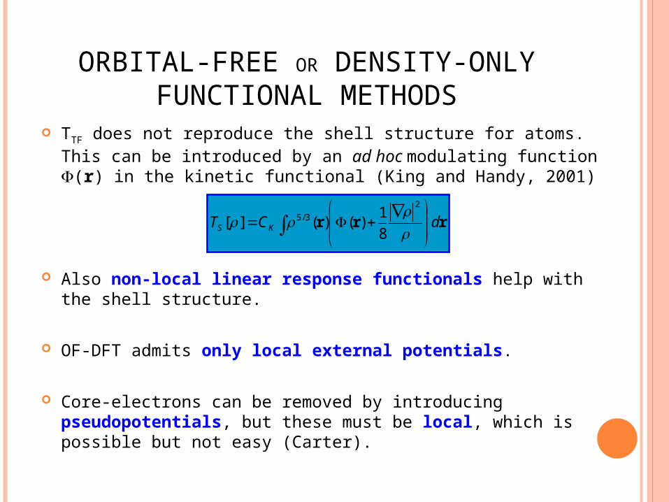
TTF does not reproduce the shell structure for atoms. This can be introduced by an ad hoc modulating function (r) in the kinetic functional (King and Handy, 2001)

Also non-local linear response functionals help with the shell structure.

OF-DFT admits only local external potentials.

Core-electrons can be removed by introducing

pseudopotentials, but these must be local, which is possible but not easy (Carter).


rrr dCT KS

2

3/5

8

1)()(][



1000

10000

1000000

100000100

High

Low

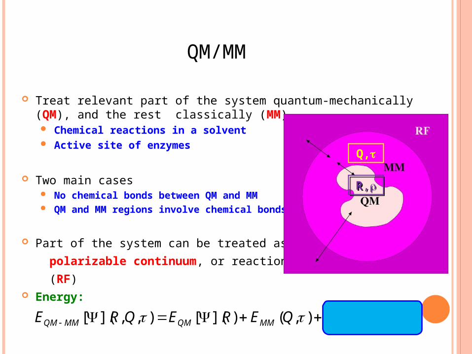
Treat relevant part of the system quantum-mechanically (QM), and the rest classically (MM). Chemical reactions in a solvent Active site of enzymes

Two main cases No chemical bonds between QM and MM QM and MM regions involve chemical bonds

Part of the system can be treated as a

polarizable continuum, or reaction field

(RF) Energy:

QM/MM

),,]([),()]([),,]([ int QREQEREQRE MMQMMMQM

R,R,

Q,

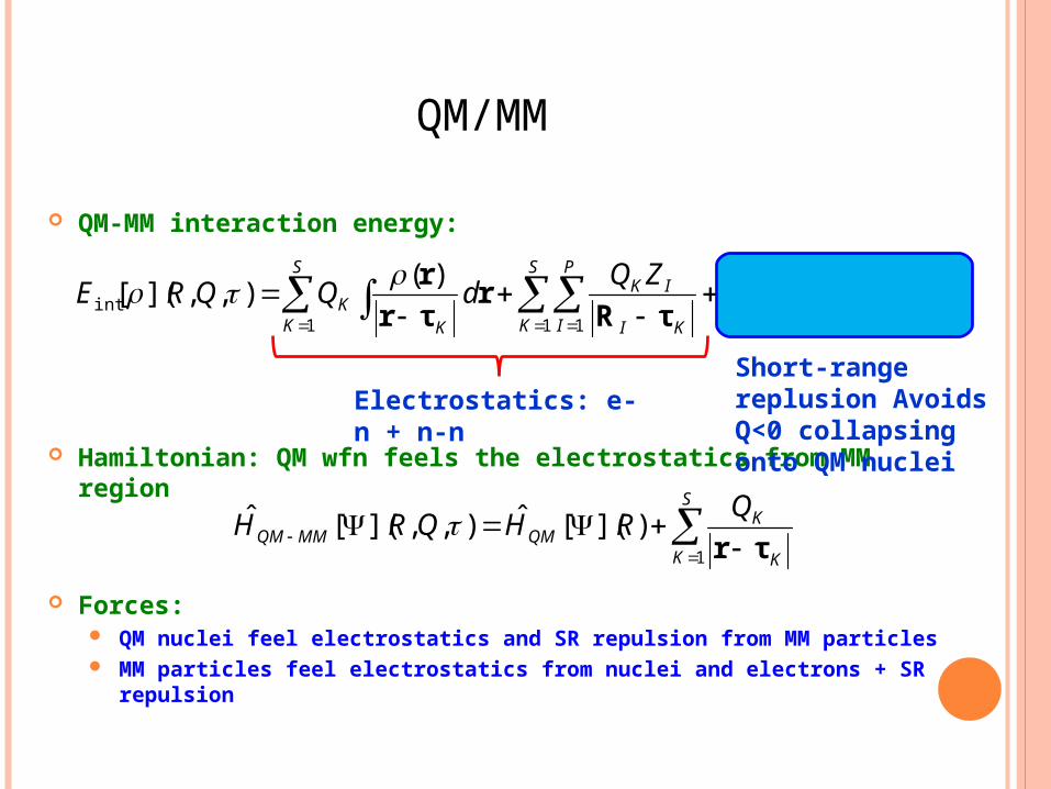
QM-MM interaction energy:

Hamiltonian: QM wfn feels the electrostatics from MM region

Forces: QM nuclei feel electrostatics and SR repulsion from MM particles MM particles feel electrostatics from nuclei and electrons + SR

repulsion

QM/MM

S

K

P

IKISR

S

K

P

I KI

IKS

K KK V

ZQdQQRE

1 11 11int

)(),,]([ τR

τRr

τr

r

Electrostatics: e-n + n-nShort-range replusion Avoids Q<0 collapsing onto QM nuclei

S

K K

KQMMMQM

QRHQRH

1

)]([ˆ),,]([ˆτr

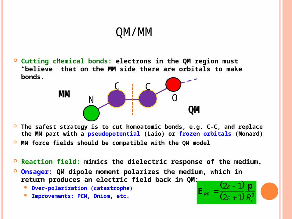
Cutting chemical bonds: electrons in the QM region must “believe” that on the MM side there are orbitals to make bonds.

The safest strategy is to cut homoatomic bonds, e.g. C-C, and replace the MM part with a pseudopotential (Laio) or frozen orbitals (Monard)

MM force fields should be compatible with the QM model

Reaction field: mimics the dielectric response of the medium. Onsager: QM dipole moment polarizes the medium, which in

return produces an electric field back in QM: Over-polarization (catastrophe) Improvements: PCM, Oniom, etc.

QM/MM

C CN O

QM

MM

312

12

cRF R

pE



1000

10000

1000000

100000100

High

Low

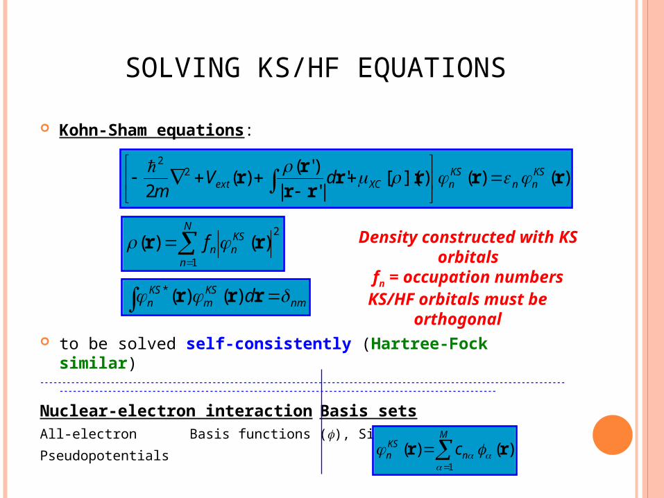
Kohn-Sham equations:

to be solved self-consistently (Hartree-Fock similar)--------------------------------------------------------------------------------------------------------------------------------------------------------------------------

------------------------------------------------

Nuclear-electron interaction Basis setsAll-electron Basis functions (), Size (M)

Pseudopotentials

)()()](['|'|

)'()(

22

2

rrrrrr

rr KS

nnKSnXCext dV

m

N

n

KSnnf

1

2)()( rr

nmKSm

KSn d rrr )()(*

Density constructed with KS orbitalsfn = occupation numbers

KS/HF orbitals must be orthogonal

)()(1

rr

M

nKSn c

SOLVING KS/HF EQUATIONS

BASIS SETS

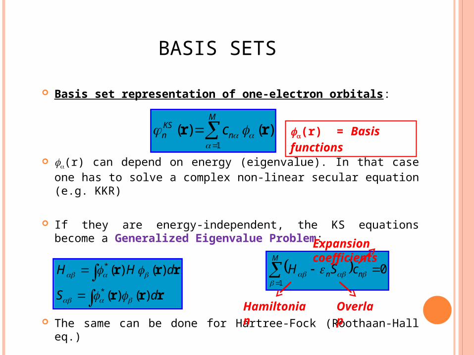
Basis set representation of one-electron orbitals:

(r) can depend on energy (eigenvalue). In that case one has to solve a complex non-linear secular equation (e.g. KKR)

If they are energy-independent, the KS equations become a Generalized Eigenvalue Problem:

The same can be done for Hartree-Fock (Roothaan-Hall eq.)

)()(1

rr

M

nKSn c

rrr

rrr

dS

dHH

)()(

)()(

*

*

01

n

M

n cSH

Hamiltonian Overlap

Expansion coefficients

(r) = Basis functions

LOCAL ORBITALS

Atom-centered basis functions:

Types: Atomic orbitals (AO) Slater-type orbitals (STO): exp(- r) Gaussian-type orbitals (GTO): exp(- r2) Numerical

Generally these are non-orthogonal

Löwdin orthogonalization:

Standard Eigenvalue Problem:

)()( II Rrr

0''1

n

M

n cIH

RI = atomic positions (can use other positions)

)( IRr )( JRr

)()('1

2/1 rr

M

S

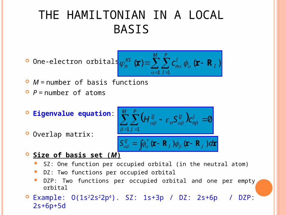
THE HAMILTONIAN IN A LOCAL BASIS

One-electron orbitals:

M = number of basis functions P = number of atoms

Eigenvalue equation:

Overlap matrix:

Size of basis set (M) SZ: One function per occupied orbital (in the neutral atom) DZ: Two functions per occupied orbital DZP: Two functions per occupied orbital and one per empty orbital

Example: O(1s22s22p4). SZ: 1s+3p / DZ: 2s+6p / DZP: 2s+6p+5d

)()(1 1

I

M P

I

In

KSn c Rrr

rRrRr dS JIIJ )()(*

01 1

Jn

M P

J

IJn

IJ cSH

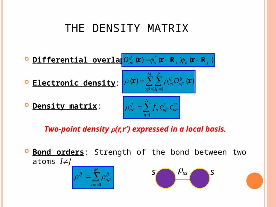
THE DENSITY MATRIX

Differential overlaps:

Electronic density:

Density matrix:

Two-point density (r,r’) expressed in a local basis.

Bond orders: Strength of the bond between two atoms IJ

)()()( *JI

IJO RrRrr

)()(1 1

rr IJM P

IJ

IJO

*

1

In

N

n

Jnn

IJ ccf

M

IJIJ

1 s sss

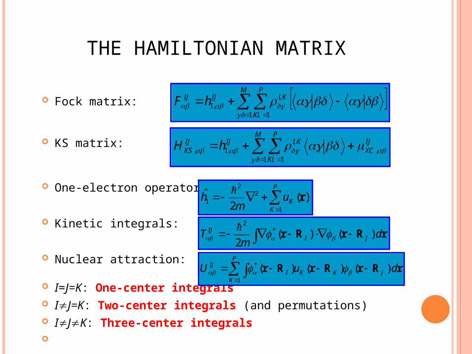
THE HAMILTONIAN MATRIX

Fock matrix:

KS matrix:

One-electron operator:

Kinetic integrals:

Nuclear attraction:

I=J=K: One-center integrals IJ=K: Two-center integrals (and permutations) IJK: Three-center integrals

M P

KL

LKIJIJ hF1 1

,1

P

KKum

h1

22

1 )(2

ˆ r

IJXC

M P

KL

LKIJIJKS hH

,

1 1,1,

rRrRr dm

T JIIJ )()(

2*

2

rRrRrRr duU JK

P

KKI

IJ )()()(1

*

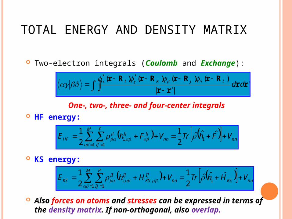
TOTAL ENERGY AND DENSITY MATRIX

Two-electron integrals (Coulomb and Exchange):

One-, two-, three- and four-center integrals HF energy:

KS energy:

Also forces on atoms and stresses can be expressed in terms of the density matrix. If non-orthogonal, also overlap.

'|'|

)()()()( **

rrrr

RrRrRrRrddLJKI

nnnnIJIJ

M P

IJ

JIHF VFhTrVFhE

ˆˆˆ2

1

2

11,1

1 1

nnKSnnIJKS

IJM P

IJ

JIKS VHhTrVHhE

ˆˆˆ2

1

2

11,,1

1 1

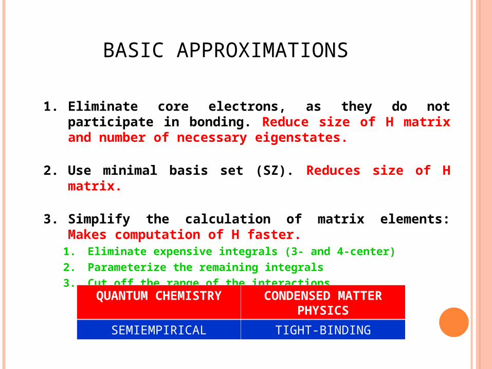
BASIC APPROXIMATIONS

1. Eliminate core electrons, as they do not participate in bonding. Reduce size of H matrix and number of necessary eigenstates.

2. Use minimal basis set (SZ). Reduces size of H matrix.

3. Simplify the calculation of matrix elements: Makes computation of H faster.

1. Eliminate expensive integrals (3- and 4-center)2. Parameterize the remaining integrals3. Cut off the range of the interactions.

QUANTUM CHEMISTRY

CONDENSED MATTER PHYSICS

SEMIEMPIRICAL TIGHT-BINDING

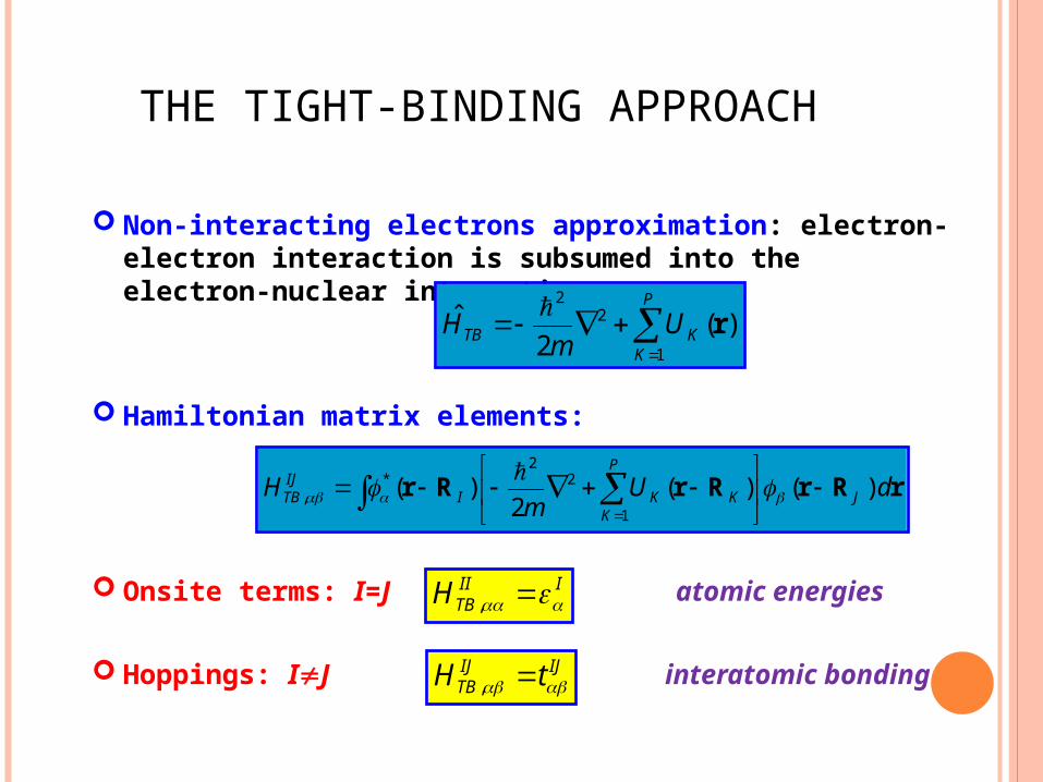
THE TIGHT-BINDING APPROACH

Non-interacting electrons approximation: electron-electron interaction is subsumed into the electron-nuclear interaction:

Hamiltonian matrix elements:

Onsite terms: I=J atomic energies

Hoppings: IJ interatomic bonding

P

KKTB U

mH

1

22

)(2

ˆ r

rRrRrRr dUm

H J

P

KKKI

IJTB )()(

2)(

1

22

*,

IIITBH ,

IJIJTB tH ,

TIGHT-BINDING: INTERPRETATION

Two-center hopping integrals:The electron feels the attraction of both nuclei

Three-center hopping integrals:The hopping between I and J is influenced by

the presence of another atom K

Onsite terms:Also influenced by the presence of neighboring atoms

)( IRr )( JRr )( IIU Rr

)( JJU Rr I J

)( IRr )( JRr

)( KKU Rr JI

K

rRrRrRr dUH IKK

P

IKI

IIITB )()()(*)0(,

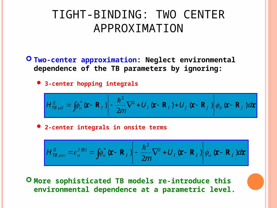
TIGHT-BINDING: TWO CENTER APPROXIMATION

Two-center approximation: Neglect environmental dependence of the TB parameters by ignoring:

3-center hopping integrals

2-center integrals in onsite terms

More sophisticated TB models re-introduce this environmental dependence at a parametric level.

rRrRrRrRr dUUm

H JJJIIIIJTB )()()(

2)( 2

2*

,

rRrRrRr dU

mH IIII

IIITB )()(

2)( 2

2*)0(

,

TIGHT-BINDING: PARAMETERIZATION

Two-center integrals are not calculated explicitly. It wouldn’t make sense, as neglected 3- and 4-center integrals have been incorporated into 2-center ones.

Instead, onsite energies and hoppings are treated as fitting parameters.

Hence, basis functions (r) become symbolic objects. Can’t reconstruct electronic density from eigenvectors.

Fitting TB parameters is a craft. A set of target properties to reproduce is selected from experiment, from ab initio or DFT calculations, or a combination of both.

Initially, it is good practice to try and fit by hand to get a feeling of the role of the various parameters. Then, since parameters interact, it is better to refine them using some automatic procedure (e.g. non-linear fitting, genetic, etc.)

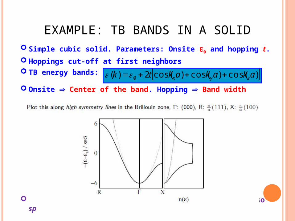
EXAMPLE: TB BANDS IN A SOLID Simple cubic solid. Parameters: Onsite 0 and hopping t.

Hoppings cut-off at first neighbors TB energy bands:

Onsite Center of the band. Hopping Band width

TB works when atomic picture is a good start: TM, also sp

)cos()cos()cos(2)( 0 akakaktk zyx

TIGHT-BINDING: ENERGY

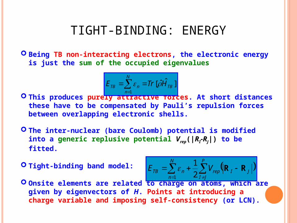
Being TB non-interacting electrons, the electronic energy is just the sum of the occupied eigenvalues

This produces purely attractive forces. At short distances these have to be compensated by Pauli’s repulsion forces between overlapping electronic shells.

The inter-nuclear (bare Coulomb) potential is modified into a generic replusive potential Vrep(|RI-RJ|) to be fitted.

Tight-binding band model:

Onsite elements are related to charge on atoms, which are given by eigenvectors of H. Points at introducing a charge variable and imposing self-consistency (or LCN).

]ˆˆ[1

TB

N

nnTB HTrE

P

JIJIrep

N

nnTB VE RR2

1

1

SELF-CONSISTENT TIGHT-BINDING

Introduce charge inbalance for each atom, defined as:

= Mulliken charge

A functional of second order in the charge inbalance can be written as (Finnis):

Lowest level of self-consistency: self-consistent charge transfer (SCCT) model.

M

III inqoutqq1

)()(

J

P

IIIJ

P

III

N

nnSCCT qqUqUE

11

2

1 2

1

2

1

Onsite Coulomb (Hubbard U)

Resists charge accumulation

ScreeningUIJ = 1/|RI-RJ|

SELF-CONSISTENT TIGHT-BINDING

Self-consistency in the entire charge distribution can be achieved by generalizing the second-order functional to multipole moments (up to some reasonable order).

Terminating the multipolar expansion at l=1 gives a polarizable tight-binding model (dipole polarizability)

SCTB Hamiltonian:

)()(2

1

2

1

2

1''

''

''

1

2

1Jml

P

JI lm ml

mllmIlmJ

P

JIIIJ

P

III

N

nnSCTB qBqqqUqUE RR

IJlm

lIlmIJIIIJTB

IJ VqUHSCTBH )(ˆ)(ˆ, R

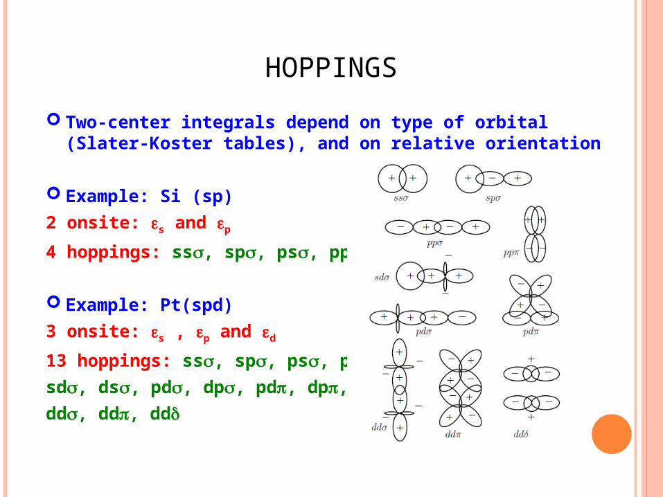
HOPPINGS

Two-center integrals depend on type of orbital (Slater-Koster tables), and on relative orientation

Example: Si (sp)

2 onsite: s and p

4 hoppings: ss, sp, ps, pp

Example: Pt(spd)

3 onsite: s , p and d

13 hoppings: ss, sp, ps, pp,

sd, ds, pd, dp, pd, dp,

dd, dd, dd

HOPPINGS AND PAIR POTENTIAL Distance dependence: hoppings decay with distance in

a way that depends on the type of orbitals

Ducastelle: exponential Harrison: Power-law

Cut-off: Decay too slow. Apply cutoff to try and retain only relevant neighbors (preferably only nearest).

Additive Multiplicative: Goodwin-Skinner-Pettifor (GSP) Multiplicative: exponential

Repulsive pair potential: Should increase faster than hoppings at small R to avoid potential collapse. Should be cut-off at similar radius of hoppings.

Attractive PP: dispersion (VDW) forces not present in electronic part. Can be added as an attractive R-6 PP.

simplified methods for electronic structure calculations jorge kohanoff queen’s university belfast...

Documents

high low slide

p slide

simplified methods

b everidge slide

electronic density

approximate wave function

electronic information

electron wave function