simplified runtime analysis of estimation of distribution algorithms

Simplified Runtime Analysis ofEstimation of Distribution Algorithms

Duc-Cuong Dang Per Kristian Lehre

University of NottinghamUnited Kingdom

Madrid, SpainJuly, 11-15th 2015

Outline

BackgroundPrevious Runtime Analyses of EDAsUnivariate Marginal Distribution Algorithm (UMDA)

Our Tool - Level-based AnalysisNon-elitist ProcessesLevel-based Theorem

Our ResultsWarm up: LeadingOnesOnemax and Feige’s Inequality

Conclusion

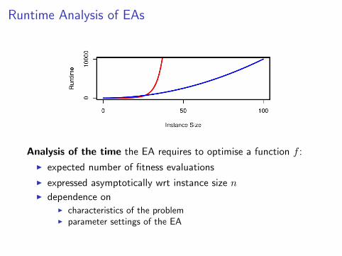
Runtime Analysis of EAs

Analysis of the time the EA requires to optimise a function f :

I expected number of fitness evaluations

I expressed asymptotically wrt instance size nI dependence on

I characteristics of the problemI parameter settings of the EA

Previous Work

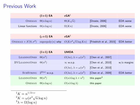
(1+1) EA cGA1

Onemax Θ(n log n) Θ(K√n) [Droste, 2006] EDA worse

Linear functions Θ(n log n) Ω(Kn) [Droste, 2006] EDA worse

(µ+1) EA cGA2

Onemax +N (0, σ2) superpoly(n) whp O(Kσ2√n logKn) [Friedrich et al., 2015] EDA better

(1+1) EA UMDA

LeadingOnes Θ(n2) O(λn), λ = ω(n2) [Chen et al., 2007]

BVLeadingOnes Θ(n2) ∞ w.o.p. [Chen et al., 2010] w/o margins

O(λn), λ = ω(n2) [Chen et al., 2010]

SubString 2Ω(n) w.o.p. O(λn), λ = ω(n2) [Chen et al., 2009] EDA better

LeadingOnes Θ(n2) O(nλ log λ+ n2) this paper3

Onemax Θ(n log n) O(nλ log λ) this paper

1K = n1/2+ε

2K = ω(σ2√n logn)3λ = Ω(logn)

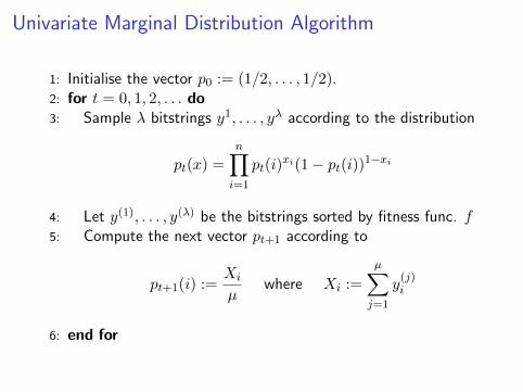
Univariate Marginal Distribution Algorithm

1: Initialise the vector p0 := (1/2, . . . , 1/2).2: for t = 0, 1, 2, . . . do3: Sample λ bitstrings y1, . . . , yλ according to the distribution

pt(x) =

n∏i=1

pt(i)xi(1− pt(i))1−xi

4: Let y(1), . . . , y(λ) be the bitstrings sorted by fitness func. f5: Compute the next vector pt+1 according to

pt+1(i) :=Xi

µwhere Xi :=

µ∑j=1

y(j)i

6: end for

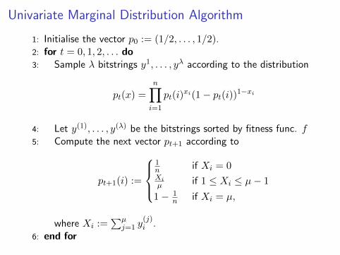
Univariate Marginal Distribution Algorithm

1: Initialise the vector p0 := (1/2, . . . , 1/2).2: for t = 0, 1, 2, . . . do3: Sample λ bitstrings y1, . . . , yλ according to the distribution

pt(x) =

n∏i=1

pt(i)xi(1− pt(i))1−xi

4: Let y(1), . . . , y(λ) be the bitstrings sorted by fitness func. f5: Compute the next vector pt+1 according to

pt+1(i) :=

1n if Xi = 0Xiµ if 1 ≤ Xi ≤ µ− 1

1− 1n if Xi = µ,

where Xi :=∑µ

j=1 y(j)i .

6: end for

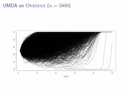
UMDA on Onemax (n = 5000)

0 10 20 30 40 50

0.0

0.2

0.4

0.6

0.8

1.0

iteration

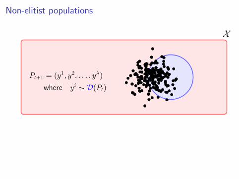
Non-elitist populations

X

Pt+1 = (y1, y2, . . . , yλ)

where yi ∼ D(Pt)

Example (UMDA)

D(P )(x) :=n∏i=1

pxii (1− pi)1−xi

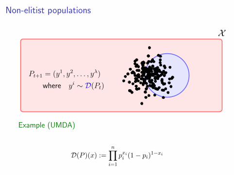
Non-elitist populations

X

Pt+1 = (y1, y2, . . . , yλ)

where yi ∼ D(Pt)

Example (UMDA)

D(P )(x) :=

n∏i=1

pxii (1− pi)1−xi

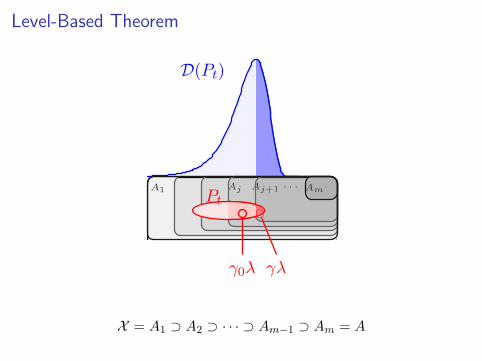
Level-Based Theorem

D(Pt)

AmA1 Aj Aj+1 · · ·Pt

γ0λ γλ

X = A1 ⊃ A2 ⊃ · · · ⊃ Am−1 ⊃ Am = A

Level-Based Theorem

≥ γ(1 + δ)

≥ zjD(Pt)

A+mA+

1A+

j A+j+1 · · ·

Pt

γ0λ γλ

Theorem (Corus, Dang, Ereemeev, Lehre (2014))

If for any level j < m and population P where

|P ∩Aj | ≥ γ0λ > |P ∩Aj+1| =: γλ

an individual y ∼ D(P ) is in Aj+1 with

Pr (y ∈ Aj+1) ≥γ(1 + δ) if γ > 0

zj if γ = 0

and the population size λ is at least

λ = Ω(ln(m/(δzj))/δ2

)then level Am is reached in expected time

O

1

δ5

m lnλ+m∑

j=1

1

λzj

.

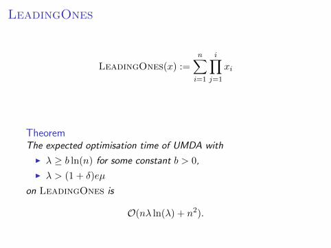
LeadingOnes

LeadingOnes(x) :=

n∑i=1

i∏j=1

xi

TheoremThe expected optimisation time of UMDA with

I λ ≥ b ln(n) for some constant b > 0,

I λ > (1 + δ)eµ

on LeadingOnes is

O(nλ ln(λ) + n2).

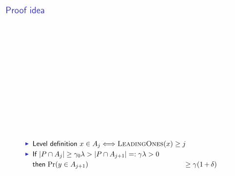
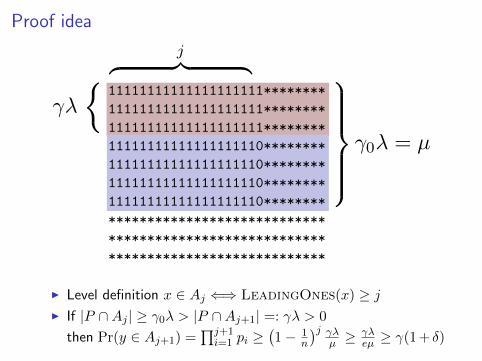
Proof idea

11111111111111111111********11111111111111111111********11111111111111111111********11111111111111111110********11111111111111111110********11111111111111111110********11111111111111111110********************************************************************************************

I Level definition x ∈ Aj ⇐⇒ LeadingOnes(x) ≥ jI If |P ∩Aj | ≥ γ0λ > |P ∩Aj+1| =: γλ > 0

then Pr(y ∈ Aj+1)

=∏j+1i=1 pi ≥

(1− 1

n

)j γλµ ≥

γλeµ

≥ γ(1 + δ)

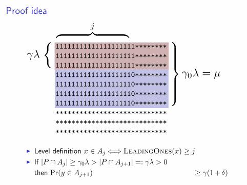
Proof idea

11111111111111111111********11111111111111111111********11111111111111111111********11111111111111111110********11111111111111111110********11111111111111111110********11111111111111111110********************************************************************************************

I Level definition x ∈ Aj ⇐⇒ LeadingOnes(x) ≥ jI If |P ∩Aj | ≥ γ0λ > |P ∩Aj+1| =: γλ > 0

then Pr(y ∈ Aj+1) =∏j+1i=1 pi ≥

(1− 1

n

)j γλµ ≥

γλeµ ≥ γ(1 + δ)

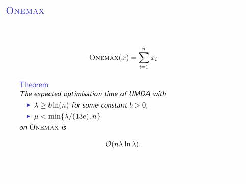
Onemax

Onemax(x) =

n∑i=1

xi

TheoremThe expected optimisation time of UMDA with

I λ ≥ b ln(n) for some constant b > 0,

I µ < minλ/(13e), non Onemax is

O(nλ lnλ).

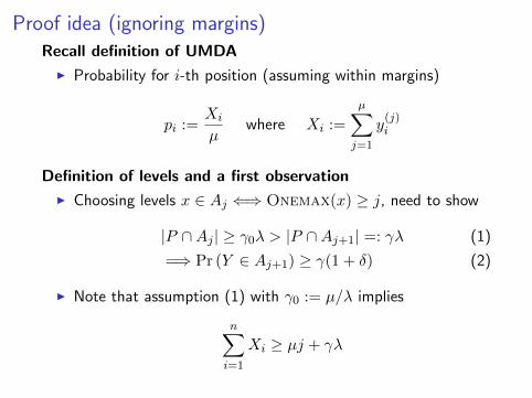
Proof idea (ignoring margins)Recall definition of UMDA

I Probability for i-th position (assuming within margins)

pi :=Xi

µwhere Xi :=

µ∑j=1

y(j)i

Definition of levels and a first observation

I Choosing levels x ∈ Aj ⇐⇒ Onemax(x) ≥ j, need to show

|P ∩Aj | ≥ γ0λ > |P ∩Aj+1| =: γλ (1)

=⇒ Pr (Y ∈ Aj+1) ≥ γ(1 + δ) (2)

I Note that assumption (1) with γ0 := µ/λ implies

n∑i=1

Xi ≥ µj + γλ

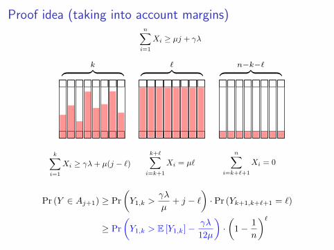
Proof idea (taking into account margins)

Pr (Y ∈ Aj+1) ≥ Pr

(Y1,k >

γλ

µ+ j − `

)· Pr (Yk+1,k+`+1 = `)

≥ Pr

(Y1,k > E [Y1,k]− γλ

12µ

)·(

1− 1

n

)`

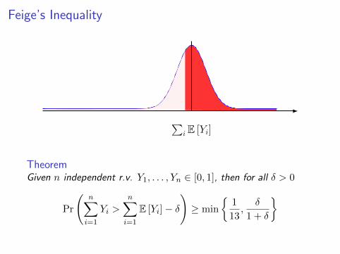
Feige’s Inequality

∑i E [Yi]

TheoremGiven n independent r.v. Y1, . . . , Yn ∈ [0, 1], then for all δ > 0

Pr

(n∑i=1

Yi >

n∑i=1

E [Yi]− δ

)≥ min

1

13,

δ

1 + δ

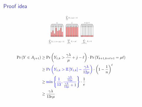
Proof idea

Pr (Y ∈ Aj+1) ≥ Pr

(Y1,k >

γλ

µ+ j − `

)· Pr (Yk+1,k+`+1 = µ`)

≥ Pr

(Y1,k > E [Y1,k]− γλ

12µ

)·(

1− 1

n

)`≥ min

1

13,

γλ12µ

γλ12µ + 1

· 1

e

≥ γλ

13eµ

≥ γ(1 + δ) if λ ≥ 13e(1 + δ)µ

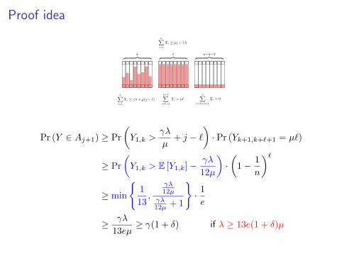
Proof idea

Pr (Y ∈ Aj+1) ≥ Pr

(Y1,k >

γλ

µ+ j − `

)· Pr (Yk+1,k+`+1 = µ`)

≥ Pr

(Y1,k > E [Y1,k]− γλ

12µ

)·(

1− 1

n

)`≥ min

1

13,

γλ12µ

γλ12µ + 1

· 1

e

≥ γλ

13eµ≥ γ(1 + δ) if λ ≥ 13e(1 + δ)µ

Conclusion and Future Work

I The recent level-based method seems well suited for EDAsI Straightforward runtime analysis of the UMDA

I Trivial analysis of LeadingOnes,smaller populations suffice, i.e., O(lnn) vs ω(n2)

I First upper bound on Onemax

I How tight are the upper bounds?I o(n lnn) on Onemax?

I Other problems and algorithmsI linear functionsI multi-variate EDAs

Thank you

The research leading to these results has received funding from theEuropean Union Seventh Framework Programme (FP7/2007-2013)under grant agreement no. 618091 (SAGE).

References

Chen, T., Lehre, P. K., Tang, K., and Yao, X. (2009).When is an estimation of distribution algorithm better than an evolutionaryalgorithm?In Proceedings of the 10th IEEE Congress on Evolutionary Computation(CEC 2009), pages 1470–1477. IEEE.

Chen, T., Tang, K., Chen, G., and Yao, X. (2007).On the analysis of average time complexity of estimation of distributionalgorithms.In Proceedings of 2007 IEEE Congress on Evolutionary Computation (CEC’07),pages 453–460.

Chen, T., Tang, K., Chen, G., and Yao, X. (2010).Analysis of computational time of simple estimation of distribution algorithms.IEEE Trans. Evolutionary Computation, 14(1):1–22.

Droste, S. (2006).A rigorous analysis of the compact genetic algorithm for linear functions.Natural Computing, 5(3):257–283.

Friedrich, T., Kotzing, T., Krejca, M. S., and Sutton, A. M. (2015).The benefit of sex in noisy evolutionary search.CoRR, abs/1502.02793.

simplified runtime analysis of estimation of distribution algorithms

Science