simulating and compiling code for the sequential quantum ... · simulating and compiling code for...

Simulating and Compiling Code for the

Sequential Quantum Random Access Machine

Rajagopal Nagarajan2 ,4 Nikolaos Papanikolaou3 ,4

Department of Computer ScienceUniversity of WarwickCoventry CV4 7ALUnited Kingdom

David Williams1

School of InformaticsCity University

London EC1V 0HBUnited Kingdom

Abstract

We present the SQRAM architecture for quantum computing, which is based on Knill’s QRAMmodel. We detail a suitable instruction set, which implements a universal set of quantum gates, anddemonstrate the operation of the SQRAM with Deutsch’s quantum algorithm. The compilationof high-level quantum programs for the SQRAM machine is considered; we present templates forquantum assembly code and a method for decomposing matrices for complex quantum operations.The SQRAM simulator and compiler are discussed, along with directions for future work.

Keywords: Quantum computation, quantum programming, quantum simulators, QRAM,compilers.

1 Email: [email protected] Email: [email protected] Email: [email protected] R. Nagarajan and N. Papanikolaou are partially supported by EPSRC grant GR/S34090and the EU Sixth Framework Programme (Project SecoQC).

Electronic Notes in Theoretical Computer Science 170 (2007) 101–124www.elsevier.com/locate/entcs

doi:10.1016/j.entcs.2006.12.0141571-0661 © 2007 Elsevier B.V. Open access under CC BY-NC-ND license.

mailto:[email protected]



http://www.elsevier.com/locate/entcs

http://creativecommons.org/licenses/by-nc-nd/3.0/

1 Introduction

The rapidly growing field of quantum computation and quantum informationis still in its infancy, largely due to the lack of a substantial, practical quan-tum computing device. However, the theoretical potential of such devices iswidely acknowledged. Presently, the only realistic avenue of investigation foran interested computer scientist is the use of quantum computer simulators.

Owing to the large state spaces of quantum–mechanical systems, a com-plete simulator of subatomic phenomena cannot be implemented efficiently ona classical computer. Nobel laureate Richard Feynman observed in 1985 that:

“. . . if a description of an isolated part of Nature with N particles requires ageneral function of N variables and if a computer simulates this by actuallycomputing or storing this function then doubling the size of Nature (N →2N) would require an exponentially explosive growth in the size of thesimulating computer.” (excerpt from [7])

Focusing on quantum mechanics in particular, Feynman points out that:

“. . . the full description of quantum mechanics for a large system with Rparticles is given by a function ψ(x1, x2, . . . , xR, t) which we call the am-plitude to find the particles at x1, x2, . . . , xR and therefore, because it hastoo many variables, it cannot be simulated with a normal computer with anumber of elements proportional to R [. . . ].”

Our goals in this paper are substantially more modest; we are interestedin local quantum computation on a finite number of quantum bits (qubits). Inparticular, we will discuss the design of a hybrid classical–quantum computerarchitecture, which we will call the Sequential Quantum Random Access Mem-ory machine, or SQRAM for short. The SQRAM design is based on Knill’sQRAM model [9]. In addition, we will define an instruction set for a hypo-thetical implementation of the SQRAM, and illustrate the operation of sucha device when running Deutsch’s algorithm for determining the balancednessof a boolean function [11]. We have implemented a simulator of the SQRAMmachine using the OpenQubit library [14]; this is described in detail in D.Williams’ M.Sc. thesis [18].

In light of recent proposals for quantum languages, including, e.g., QPL [15],QCL [12], CQP [8] and qSpec [13], we feel it is in order to consider compilationof high–level quantum programs; we discuss techniques for this and present acompiler we have developed for a subset of QPL.

We begin with a summary of basic quantum computing concepts. We willthen proceed to describe the proposed SQRAM architecture and instructionset; to illustrate the instruction set, we show how Deutsch’s algorithm would

R. Nagarajan et al. / Electronic Notes in Theoretical Computer Science 170 (2007) 101–124102

be implemented in assembly language for the SQRAM. Finally, we will turnto compilation of high–level quantum programs in QPL, a functional quantumprogramming language.

2 Related Work

Currently several quantum simulators are available, including tools for an-alyzing quantum circuits and interpreters for quantum programming lan-guages [3,12]. The work presented here is also closely related to that describedin [2,12,15], which deals with the issues involved with the design of quantumprogramming languages. Our work develops a more complete suite of toolsconsisting of separate (but interacting) parts for compilation and simulation;it also allows compiled code to be stored.

In [16], a multi-layer framework is defined, which models different levels ofabstraction for a quantum computer simulator; however, the authors accountfor specific aspects of physical implementation; on the contrary, we simply relyon the hypothesis that the proposed system architecture may be implementedwith present–day hardware, and do not concern ourselves with details of thephysics.

3 Quantum Computing Fundamentals

A few preliminaries are in order; we are assuming no prior knowledge of quan-tum computing.

A quantum bit or qubit is a physical system which has two basis states,conventionally written |0〉 and |1〉, corresponding to one-bit classical values.These could be, for example, spin states of an electron or polarization statesof a photon, but we do not consider physical details. According to quan-tum theory, a general state of a quantum system is a superposition or linearcombination of basis states. A qubit has state α|0〉 + β|1〉, where α and βare complex numbers such that |α|2 + |β|2 = 1; states which differ only by a(complex) scalar factor with modulus 1 are indistinguishable. States can berepresented by column vectors:

[αβ

]= α|0〉 + β|1〉 Formally, a quantum state

is a unit vector in a Hilbert space, i.e. a complex vector space equipped withan inner product satisfying certain axioms.

The basis {|0〉, |1〉} is known as the standard basis. Other bases are some-times of interest, especially the diagonal (or dual, or Hadamard) basis con-sisting of the vectors

|+〉 =1√2(|0〉 + |1〉) and |−〉 =

1√2(|0〉 − |1〉)

R. Nagarajan et al. / Electronic Notes in Theoretical Computer Science 170 (2007) 101–124 103

Evolution of a closed quantum system can be described by a unitary trans-formation. If the state of a qubit is represented by a column vector then aunitary transformation U can be represented by a complex-valued matrix (uij)such that U−1 = U∗, where U∗ is the conjugate-transpose of U (i.e. elementij of U∗ is uji). U acts by matrix multiplication:

⎡⎣α′

β ′

⎤⎦ =

⎡⎣u00 u01

u10 u11

⎤⎦

⎡⎣α

β

⎤⎦

A unitary transformation can also be defined by its effect on basis states,which is extended linearly to the whole space. For example, the Hadamardoperator is defined by

|0〉 �→ |+〉 = 1√2|0〉 + 1√

2|1〉

|1〉 �→ |−〉 = 1√2|0〉 − 1√

2|1〉

which corresponds to the matrix H = 1√2

⎡⎣1 1

1 −1

⎤⎦. The Pauli operators,

denoted by σ0, σ1, σ2, σ3, are defined by

σ0 =

⎡⎣1 0

0 1

⎤⎦ σ1 =

⎡⎣0 1

1 0

⎤⎦

σ2 =

⎡⎣0 −i

i 0

⎤⎦ σ3 =

⎡⎣1 0

0 −1

⎤⎦

Measurement plays a key role in quantum physics. If a qubit is in stateα|0〉 + β|1〉 then measuring its value gives the result 0 with probability |α|2(leaving it in state |0〉) and the result 1 with probability |β|2 (leaving it instate |1〉).

For example, if a qubit is in state |+〉 then a measurement (with respectto the standard basis) gives result 0 (and state |0〉) with probability 1

2, and

result 1 (and state |1〉) with probability 12. If a qubit is in state |0〉 then a

measurement gives result 0 (and state |0〉) with probability 1.

To go beyond single-qubit systems, we consider tensor products of spaces(in contrast to the Cartesian products used in classical systems). If spacesU and V have bases {ui} and {vj} then U ⊗ V has basis {ui ⊗ vj}. Inparticular, a system consisting of n qubits has a 2n-dimensional space whose


standard basis is |00 . . . 0〉 . . . |11 . . . 1〉. We can now consider measurementsof single qubits or collective measurements of multiple qubits. For example,a 2-qubit system has basis |00〉, |01〉, |10〉, |11〉 and a general state is α|00〉 +β|01〉 + γ|10〉 + δ|11〉 with |α|2 + |β|2 + |γ|2 + |δ|2 = 1. Measuring the firstqubit gives result 0 with probability |α|2 + |β|2 (leaving the system in state

1√|α|2+|β|2 (α|00〉 + β|01〉)) and result 1 with probability |γ|2 + |δ|2 (leaving

the system in state 1√|γ|2+|δ|2 (γ|10〉 + δ|11〉)); in each case we renormalize

the state by multiplying by a suitable scalar factor. Measuring both qubitssimultaneously gives result 0 with probability |α|2 (leaving the system in state|00〉), result 1 with probability |β|2 (leaving the system in state |01〉) and so on;the association of basis states |00〉, |01〉, |10〉, |11〉 with results 0, 1, 2, 3 is justa conventional choice. The power of quantum computing, in an algorithmicsense, results from calculating with superpositions of states; all of the states inthe superposition are transformed simultaneously (quantum parallelism) andthe effect increases exponentially with the dimension of the state space. Thechallenge in quantum algorithm design is to make measurements which enablethis parallelism to be exploited; in general this is very difficult.

The controlled not (CNOT) operator on pairs of qubits performs the map-ping:

|00〉 �→ |00〉|01〉 �→ |01〉|10〉 �→ |11〉|11〉 �→ |10〉

which can be understood as inverting the second qubit (the target) if and onlyif the first qubit (the control) is set. The action on general states is obtainedby linearity.

Systems of two or more qubits may be in entangled states, meaning thatthe states of the qubits are correlated. For example, consider a measurementof the first qubit of the state 1√

2(|00〉+ |11〉). The result is 0 (and the resulting

state is |00〉) with probability 12, or 1 (and the resulting state is |11〉) with

probability 12. In either case, a subsequent measurement of the second qubit

gives a definite, non–probabilistic result which is identical to the result of thefirst measurement. This is true even if the entangled qubits are physicallyseparated. Entanglement illustrates the key difference between the use of thetensor product (in quantum systems) and the Cartesian product (in classicalsystems): an entangled state of two qubits is one which cannot be expressed asa tensor product of single-qubit states. The Hadamard and CNOT operators


can be combined to create entangled states:

CNOT((H ⊗ I)|00〉) =1√2(|00〉 + |11〉)

4 The SQRAM Machine

In this section we propose a system architecture for a hybrid classical–quantumcomputer, consisting of a classical computing machine with control over apurely quantum–mechanical component. Such a device, termed a QRAMmachine, was proposed by Knill in [9].

The classical component comprises a Central Processing Unit (CPU), aclassical data store (DS) and a program store (PS). The quantum–mechanicalcomponent is divided into a Quantum Hardware Interface (QHI), a quantummemory register, and a means of manipulating its contents; note that ourdiscussion remains independent of particular hardware implementations andassociated physical details.

Figure 1 illustrates the overall design of the SQRAM machine, includingboth the classical component and the quantum component. We will nowdescribe the details of this design, including its operating cycle and instructionset.

4.1 The Classical Component

The classical component has two distinct memory locations, one for programsand one for data. We have chosen to deviate slightly from the conventionalVon Neumann model, where programs are treated in the same way, and inthe same location, as the data they manipulate. The CPU keeps track of thecurrent instruction in a program through the program counter, which indexesa location in the program store.

The CPU also contains an Arithmetic–Logic Unit, for evaluating classicalexpressions, and a control unit, for other operations. The CPU does notcontain any registers, since all operations are performed within the data store.

The data store operates a stack–based model for evaluation of expressionsand the allocation of variables; this fits well with the functional programmingparadigm and simplifies code generation for the compiler. Global data (ifapplicable) is stored from the address 0x0000 while the local base points tothe the beginning of the data local to the current function (this is modifiedas functions are entered and left). Stack top points just after the end of thevalid data area.

Table 1 details the principal instructions used to control the classical com-


ponent of the SQRAM and describes the effect of each instruction in an al-gorithmic notation. The notation includes the symbols st (the Stack Top), lb(the Local Base), pc (the value of the Program Counter), DS[i] (the contentsof location i in the Data Store), and PS[i] (the contents of location i in theProgram Store).

The operating cycle of the SQRAM is as follows. Program execution be-gins with the program counter, local base, and stack top all initialized to 0.An instruction is retrieved from the location given by the program counter andexecuted, the process is then repeated. Most instructions cause the programcounter to be incremented but some (such as jumping and halting instruc-tions) have different effects for a listing of the available classical instructions).Program execution is finished once the program counter goes past the end ofthe program store.

Logic UnitArithmetic

UnitControl

CounterProgram

Central Processing Unit

Key: Data store out of scope

Data store not yet allocated

Data store in use

Quantum

Register

Local

Stack

0x0F

Top

Base

0x00

Read/Write

ProgramStore

Instructions

Quantum Component

Results Of Measurements

Operations

Quantum StateInteraction With

Classical Component

QuantumHardwareInterface

0x000F

0xFFF0

Local Base

StackTop

0x0000

0xFFFF

Data Store

Fig. 1. Design of the SQRAM machine


Instruction Effect

ADD

st ← st − 1

DS[st − 1] ← DS[st − 1] + DS[st]

pc ← pc + 1

HALT pc ← size(PS)

JUMPZ address

st ← st − 1

if(DS[st − 1] = 0) :

pc ← address

else :

pc ← pc + 1

LOAD offset

DS[st] ← DS[lb + offset ]

st ← st + 1

pc ← pc + 1

LOADLvalue

DS[st] ← value

st ← st + 1

pc ← pc + 1

SAVE offset

st ← st − 1

DS[lb + offset ] ← DS[st]

pc ← pc + 1

SUBTRACT

st ← st − 1

DS[st − 1] ← DS[st − 1] − DS[st]

pc ← pc + 1

Table 1SQRAM Machine Classical Instruction Set

4.2 The Quantum Component

The quantum component of the SQRAM consists of a quantum register anda Quantum Hardware Interface (QHI), which receives instructions from theCPU and manipulates qubits accordingly. Figure 2 illustrates the stages of a


Repeat if Necessary

and LoadingInitialisation Quantum State

EvolutionMeasurement

of StateChecking

Fig. 2. SQRAM Operating Cycle

typical quantum algorithm.

In the first stage of Figure 2, the hardware resets the qubits to the |0〉state and then applies some transformation to place them in the desired ini-tial state. The second stage is where the manipulation of the quantum stateactually takes place. After the computation is complete, the result is mea-sured; each measured qubit yields a binary value {0, 1} which is passed to theCPU and can then be used for conditional control purposes. The final stagechecks the validity of the result and repeats the computation if necessary.Incorrect results may occur, either due to hardware problems such as deco-herence, which damages quantum states, or due to the probabilistic nature ofquantum algorithms.

As was explained in Section 3, the state is transformed by applying asequence of operations to it; these may operate on an arbitrary number ofqubits and the only restriction is that they must be unitary. While this isaccurate from a theoretical point of view it is at the present time very difficultto implement arbitrary operations on arbitrary numbers of qubits. Fortunatelyit is known that there is a small set of operations (actually an infinite numberof such sets) which is universal in that it is able to approximate an arbitraryoperation to any given accuracy [11].

We now introduce the operations which make up one of these universalsets (known as the standard set). The first operation is the Controlled–NOT(CNOT), which we described previously. This operation can be combined witharbitrary single qubit operations to exactly implement any quantum operationon an arbitrary number of qubits.

To complete the standard set it is necessary to approximate arbitrary singlequbit operations. Within the standard set this is done with the HadamardOperator (denoted by H), the Phase Operator (S) and the π/8 operator.We use the standard set as the basis for the instruction set of the SQRAM,along with instructions for measurement and initialisation, and a classicalset of instructions for control purposes. We also include an instruction forperforming arbitrary operations on single qubits. The ‘quantum instructions’for the SQRAM are summarized in Table 2. Special notation used in this tableincludes the symbols target (for target qubit), control (for control qubit), andinvert (indicates the CNOT is active when the control is in the state |0〉 rather


Instruction Effect

AQBIT

QR[qst] ← |0〉qst ← qst + 1

pc ← pc + 1

CNOT target

control invert

QR[target] ← target × cnot(control, invert, . . .)

pc ← pc + 1

GATE target

a b c d

QR[target] ← target × gate(a, b, c, d)

pc ← pc + 1

HDMD targetQR[target] ← target × gate( 1√

2, 1√

2, 1√

2,− 1√

2)

pc ← pc + 1

MSRE target

DS[st] ← measure(target)

st ← st + 1

pc ← pc + 1

PHASE targetQR[target] ← target × gate(1, 0, 0, i)

pc ← pc + 1

PI targetQR[target] ← target × gate(1, 0, 0, eiπ/4)

pc ← pc + 1

Table 2SQRAM Machine Quantum Instruction Set

than |1〉); otherwise, the notation is mostly self–explanatory.

4.3 Deutsch’s Algorithm on the SQRAM Machine

We now present an example of a program written for the SQRAM machine.We will be using Deutsch’s algorithm as given in [5]; that reference should beconsulted for further details of the algorithm, as the description given herewill be necessarily brief.

We are presented with a black–box which performs some function f(x) ona single bit x. There are four possible functions which f(x) could perform,these being f(x) = 0, f(x) = 1, f(x) = NOT (x), and f(x) = x. Of these thefirst two are called constant because they always give the same result, whilethe second two are called balanced because half the inputs result in 0 and half


result in 1. The problem is to determine, using as few function evaluations aspossible, whether f(x) is constant or balanced.

If done classically, this requires two function evaluations, one with an inputof 0 and the other with an input of 1, and a comparison of the results. However,using Deutsch’s algorithm on a quantum computer it is possible to use just onefunction evaluation. Note that if the function is constant then f(0)⊕f(1) = 0,while if it is balanced then f(0)⊕ f(1) = 1. Using the circuit in Figure 3 it ispossible to evaluate f(0) ⊕ f(1) with out ever finding out the values of f(0)and f(1).

H

H

Uf

|0>

|1>

H x

y

Fig. 3. A Circuit Implementing Deutsch’s Algorithm.

An implementation, for the SQRAM machine, of Deutsch’s algorithm fortesting the balancedness of the NOT gate is given in Figure 4. The NOT gateis balanced, so the result of evaluating f(0) ⊕ f(1) should be 1.

Compared to the circuit representation, this code involves additional ini-tializations as all qubits are automatically placed in state |0〉. The secondqubit actually needs to be placed in state |1〉; this is achieved using the NOToperation. Note that the NOT operation has been realized using the GATE

instruction; it could have been implemented just as well using a CNOT withno controls. The operation Uf is a reversible form of an f(x)–controlled–NOT ;it performs the mapping |x〉|y〉 → |x, y ⊕ f(x)〉. The f(x)–controlled–NOToperation is, in our example, a NOT–controlled–NOT which in turn is im-plemented as a CNOT with its control inverted to trigger when in the state|0〉.

The example mostly illustrates quantum instructions; the functions per-formed by classical instructions should be familiar to most readers. The onlyclassical instruction used in this example is SAVE, which stores the result ofthe measurement at the top of the classical stack. Further code could condi-tionally jump based on this value to give feedback to the user.

4.4 Simulating the SQRAM

In order to evaluate and analyze the design of the SQRAM, we have developeda software simulator. Simulation of quantum mechanical systems is knownto be a highly complex problem (as discussed in the Introduction), and soour simulator handles only a relatively small number of qubits. There are,of course, several known quantum algorithms which only make use of a few


AQBIT ;allocate initial qubits

AQBIT

GATE 0x01 0.0 0.0 1.0 0.0 1.0 0.0 0.0 0.0 ;initialise second qubit to 1

HDMD 0x00 ;apply Hadamards

HDMD 0x01

CNOT 0x01 1 0 1 ;apply the CNOT gate

HDMD 0x00 ;the last Hadamard

MSRE 0x00 ;measure the result

SAVE 0x00 ;save to address 0x00 for later

Fig. 4. SQRAM Assembly Program Implementing Deutsch’s Algorithm for the NOT gate

qubits; these we have already succeeded in modelling.

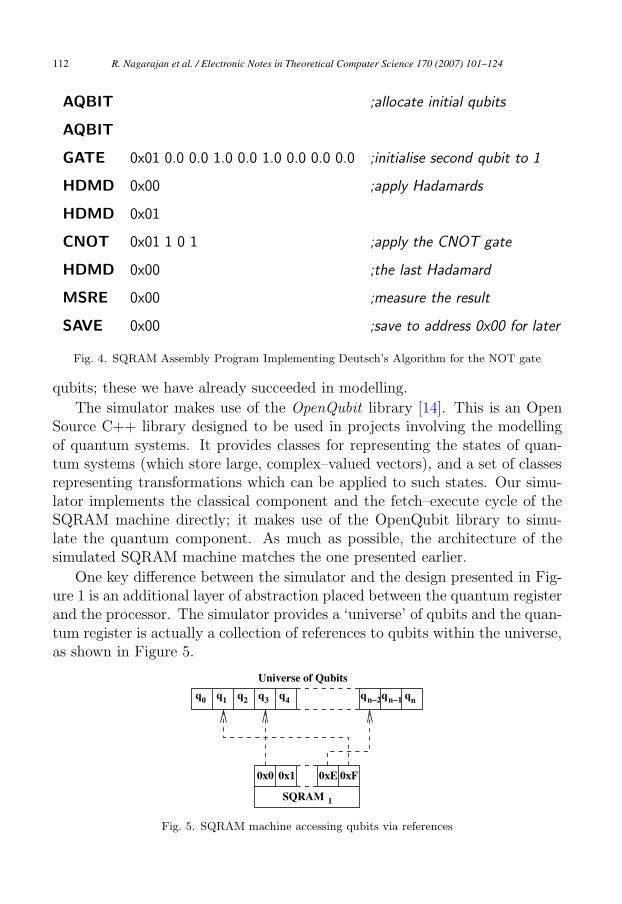
The simulator makes use of the OpenQubit library [14]. This is an OpenSource C++ library designed to be used in projects involving the modellingof quantum systems. It provides classes for representing the states of quan-tum systems (which store large, complex–valued vectors), and a set of classesrepresenting transformations which can be applied to such states. Our simu-lator implements the classical component and the fetch–execute cycle of theSQRAM machine directly; it makes use of the OpenQubit library to simu-late the quantum component. As much as possible, the architecture of thesimulated SQRAM machine matches the one presented earlier.

One key difference between the simulator and the design presented in Fig-ure 1 is an additional layer of abstraction placed between the quantum registerand the processor. The simulator provides a ‘universe’ of qubits and the quan-tum register is actually a collection of references to qubits within the universe,as shown in Figure 5.

q4q3q2q1q0 qnn−1qn−2q

Universe of Qubits

0x0 0xF0x1 0xE

SQRAM 1

Fig. 5. SQRAM machine accessing qubits via references


5 Compiling High-Level Languages for the SQRAM

It is impractical to write large programs by hand using the assembly languageinstructions presented in the previous section; this is time consuming anderror prone. The emergence of quantum programming languages, which canautomatically be compiled into corresponding machine code, facilitates thetask of ‘quantum programming’ significantly.

A quantum programming language provides an elegant mixture of classicalcontrol structures and quantum operations; this is something which is verydifficult, if not impossible, to implement in the standard quantum circuitmodel. The use of quantum programming languages fits in well with themodel of computation used by our SQRAM machine (and by most quantumalgorithms). This computational model is more familiar to computer scientiststhan the circuit model, and we expect it to greatly ease the development ofnew quantum algorithms.

In this section, we consider high–level quantum programming languagesand how programs written in such languages may be translated into assemblycode for the SQRAM machine. We begin by identifying certain desirablecharacteristics and particularities of such languages, and then we proceed todiscuss Selinger’s QPL [15], a functional quantum programming language. Wehave implemented a translation from a subset of QPL to SQRAM assemblycode, which is also described briefly.

5.1 Quantum Programming Language Requirements

According to [2,9,15], the desired features of high–level quantum programminglanguages are:

Classical Characteristics: Many years of research on classical languageshave identified properties such as a clean syntax and intuitive set of key-words as being important for high–level languages.

Completeness: A quantum programming language should be universal, sothat it can represent all quantum algorithms. This gives it the same expres-sive power as the quantum circuit model.

Expressivity: The language should present the programmer with a suffi-cient set of primitives and constructs to allow quantum programs to beconstructed easily.

Separability: It should be simple to separate those parts of the programwhich are quantum–mechanical in nature from those parts which are clas-sical, as this can simplify compilation and execution of a given program.

Hardware Independence: A quantum programming language should be


portable, i.e., independent of a particular hardware platform. A languageshould be kept as general as possible, perhaps even using the QuantumTuring machine as its target platform.

Extension of Classical Languages: Quantum programming languages whichextend known classical languages are likely to find a wider user base thancompletely new languages.

5.2 Particularities of Quantum Systems Affecting Language Designs

The inability to clone an unknown quantum state has a direct effect on thebehavior of statements which involve assignment; these include direct assign-ment and passing values to functions. Because it is not possible to actuallycopy the value many languages make use of references and hence have manyvariables pointing to the same qubit. Other languages may forbid the directassignment of quantum variables.

Although, as noted previously, it is not possible to assign one qubit toanother, it is possible to assign a qubit to a classical bit; this involves animplicit measurement. Unlike classical programming, this will modify thevariable on the right hand side of the assignment, and it is not possible torestore the previous value.

It is possible for two qubits identified by separate variable names to becomeentangled, so that the manipulation of one variable has an effect on the other.There is no analogy to this in classical programming, but this is more of anissue for the programmer than it is for the language designer.

5.3 A Functional Quantum Programming Language: QPL

There are several languages which meet the requirements set out previouslyto varying degrees [2,9,12]. Our work focuses on one in particular, PeterSelinger’s QPL [15], due to its elegant design and its suitability for implemen-tation on the SQRAM machine.

Selinger identifies the static type system as being one of the key features ofQPL; this allows the syntax to enforce certain requirements of quantum theory,such as the no–cloning theorem. As well as the usual control constructs, suchas loops and conditional statements, QPL allows the definition of recursivefunctions. This is useful when operating on lists and trees, which in QPL, maycontain quantum as well as classical data. The syntax of QPL is reproducedfrom [15] in Figure 6.


QPLTerms P, Q :: = new bit b := 0

| new qbit q := 0

| discard x | b := 0 | b := 1

| q1, . . . , qn∗ = S | skip | P ; Q

| if b then P else Q

| measure q then P else Q

| while b do P

| proc X : Γ → Γ′{P} in Q

| y1, . . . , ym = X(x1, . . . , xn)

Fig. 6. The syntax of Peter Selinger’s QPL, reproduced from [15].

5.4 Code Templates for Quantum Operations

Code generation, for our purposes, is the process of producing machine in-structions for each of the nodes in the abstract syntax tree corresponding to ahigh–level program. We have designed code templates for the quantum con-structs in the QPL language, and we have also considered the decompositionof large operations, so they may be implemented directly using the limitednumber of instructions available.

Code templates are used in compilers to provide a set of assembly instruc-tions which correspond to a particular construct in the source program, suchas an expression, a loop, or a variable declaration. We will now define codetemplates for those constructs which are quantum in nature; we will not givedetails of classical constructs here. Specifically, we will cover the declarationof quantum data, its manipulation and eventual measurement. The mappingof a high–level QPL construct to the corresponding SQRAM assembly code isexpressed as a function

Translation : QPLTerms �→ SQRAMTerms

In QPL, a new qubit is declared using the statement:

(new qbit q := 0)

This allocates a new qubit, referred to by the variable name q, and initializesit to the state |0〉. To implement this we simply use the AQBIT instruction:

Translation[(new qbit q:=0)] = AQBIT


A transformation is applied to a quantum data type using the ∗ = operator.For example, the built-in unitary transformation U could be applied to q asfollows: (q∗ = U). There are two situations to consider here. Firstly U mightbe a single qubit operation which we wish to implement directly using theGATE instruction. This becomes:

Translation[(q∗ = U)] = GATE q U

Alternatively U might be a multi–qubit operation (in which case q wouldneed to be a multi–qubit data type), or it might be a single qubit operationwhich we wish to decompose into gates from the universal set of operations.Either way, we move into the decomposition process which is discussed inSection 5.5.

Measurement is the most complex of the code templates (assuming wedon’t get involved with decomposition when manipulating quantum types).QPL performs measurement by the following statement:

measure q then P else Q

A measurement is performed on the qubit q. If the result of the measure-ment is |1〉 then the command corresponding to P is executed, otherwise thecommand corresponding to Q is executed. The code template for this looksas follows:

Translation[measure q then P else Q]=

MSRE q ; Perform the measurement

JUMPZ else ; If result is 0, jump to else

P ; Execute command P if result is not 0.

LOADL 0 ; Unconditionally jump to end,

JUMPZ end ; by loading 0 and jumping to 0.

else: Q ; Execute command Q.

end: ; End.

If the measurement of q gives a value of 1 then the JUMPZ instruction isignored and the program proceeds to execute P before unconditionally jump-ing over the code to execute Q. On the other hand, if q is measured as 0 thefirst JUMPZ jumps over the execution of P straight to the point where Q isexecuted.


U11 U12 U1n

U21

Un1

U22 U2n

Un2 Unn

Generate aset of two

level unitarymatrices

implementation by controlled

Generate sequenceof CNOT gates to allow

single qubit operation

Implement controlled unitary operation withsingle qubit operations

and CNOT’s

X

Stage 1Input Stage 2

Stage 3 Stage 4 Output

Generate primitiveoperations to

approximate singlequbit operation.

Fig. 7. Decomposition of an Arbitrary Unitary Matrix

5.5 Decomposition of Operator Matrices

In Section 4.2 we discussed the principle of universality, stating that any quan-tum operation can be broken down and implemented in terms of a small set ofuniversal gates. Hence our SQRAM machine only provides operations corre-sponding to these universal gates and it is the job of the compiler to performthe decomposition. This decomposition is a complex process and work hasbeen done on it by a variety of different people and research groups. We bringthis work together to form a complete compilation process and provide ananalysis of its efficiency.

5.5.1 Overview

Decomposing a matrix into primitive operations is a multistage process (out-lined in Figure 7); each of the stages shown is described in the followingsections. The mathematical proofs for the validity of each stage of the processare well established and work has previously been done looking at the optimalnumber of gates which can be used to approximate a given unitary matrix[11]. Therefore this work focuses on designing algorithms to implement theprocess and performing classical efficiency analysis on these algorithms. It isto our knowledge the first system to implement the complete process fromarbitrary operations to quantum byte–code within a compiler.

A working compiler has been implemented to test the concepts presented inthe following sections but we will not discuss its implementation here. For de-tails of this including design approaches, examples, and sample output pleaserefer to [18].


5.5.2 Generating Two-Level Unitary Matrices

Two-level unitary matrices are those which act non-trivially on only 2 vectorcomponents of the system state; that is ,when the vector is multiplied by thematrix only two elements are changed as most elements in the matrix areidentity. Such a matrix has a structure as follows:

Rk =

⎡⎢⎢⎢⎢⎢⎢⎢⎢⎢⎢⎢⎢⎢⎢⎢⎢⎢⎢⎢⎢⎢⎣

. . ....

......

......

...

· · · 1 0 0 · · · 0 0 0 · · ·· · · 0 α 0 · · · 0 γ 0 · · ·· · · 0 0 1 · · · 0 0 0 · · ·

......

.... . .

......

...

· · · 0 0 0 · · · 1 0 0 · · ·· · · 0 β 0 · · · 0 δ 0 · · ·· · · 0 0 0 · · · 0 0 1 · · ·

......

......

......

. . .

⎤⎥⎥⎥⎥⎥⎥⎥⎥⎥⎥⎥⎥⎥⎥⎥⎥⎥⎥⎥⎥⎥⎦

(1)

The initial step is to decompose the original matrix U of side length s intoa sequence of two-level unitary matrices (also of side length s). The productof the matrices in this sequence must be equal to the input matrix U , sothat applying them to the system in the correct order has the same effect asapplying U .

Performing this decomposition is not only necessary for the next stage, itis also a result in its own right. A description of a technique for implementingsuch transformations with beam–splitter devices is presented in [20], with theresult that simply performing this stage could bring arbitrary operations closerto being realizable.

We will not go deeply into the mathematics involved as it can becomereasonably complicated; for a coverage of this see [20,18,11]. It has beenobserved [11] that such a process will decompose the original matrix into at

most s(s−1)2

two level matrices. However, no analysis of the efficiency of suchan algorithm was provided and it is a useful result to determine this. In [18]we make some assumptions about the efficiency of variations and show thecomplexity to be approximately Θ(n5). This is clearly not a fast algorithm,and it should be noted that the previous analysis was with respect to thesize of the matrix (which is exponential in the size of the system). Hence thealgorithm requires exponential time overall, but it should also be remembered


that it will typically be operating on small values of n, corresponding to asmall number of qubits. Also, the difficulty in performing this decompositionmakes it clear that it is necessary to have a quantum byte–code which can bestored as it too difficult to generate in real time.

5.5.3 Generating Controlled Unitary and CNOT Gates

We obtain from the previous stage a set of two level unitary matrices, forexample a matrix of the form:

U =

⎡⎢⎢⎢⎢⎢⎢⎣

α 0 0 γ

0 1 0 0

0 0 1 0

β 0 0 δ

⎤⎥⎥⎥⎥⎥⎥⎦

(2)

A matrix such as this acts on two components of the system (in this partic-ular case it acts on |00〉and |11〉), and leaves the other components unaffectedas follows:

⎡⎢⎢⎢⎢⎢⎢⎣

|00〉|01〉|10〉|11〉

⎤⎥⎥⎥⎥⎥⎥⎦

U−→

⎡⎢⎢⎢⎢⎢⎢⎣

α |00〉 + γ |11〉|01〉|10〉β |00〉 + δ |11〉

⎤⎥⎥⎥⎥⎥⎥⎦

(3)

We wish to implement this matrix in terms of a controlled single qubitoperation, or Controlled–U gate, but note that a single qubit operation cannotact on both |00〉 and |11〉 as they differ by more than one bit. Therefore weuse a series of CNOT gates (in this simple case the series contains just onegate) to swap states around such that the target states are adjacent to eachother. The Controlled-U is then applied to the one bit which still differs, andthe reverse series of CNOT gates is used to arrange the states back to theiroriginal position.

To clarify this procedure, the operation given by Equation 2 is implementedby the circuit in Figure 8, where T is the sub–matrix of U given by:

T =

⎡⎣α γ

β δ

⎤⎦ (4)


T

Fig. 8. Circuit implementing Equation 2.

Note that the CNOT gates are active when the control qubit is |0〉, ratherthan the more conventional |1〉. The problem then is how to generate the seriesof CNOT gates which rearrange the computational states in the appropriateway. A solution involving the use of Gray codes is covered by [11] and adescription within the context of our compiler is provided by [18].

5.5.4 Implementing Controlled Unitary Gates

The output from the procedure described in Section 5.5.3 consists of two typesof gates; Controlled–NOT gates and Controlled–U gates. Our SQRAM ma-chine is able to directly implement Controlled–NOT gates through the CNOTinstruction, but Controlled–U gates require further decomposition. This sec-tion shows briefly how this is done, building on work presented by Barenco etal. in [1]. Note that we will only consider Controlled–U gates with a singlecontrol; for details of how the techniques apply to more controls please consult[18].

Barenco et al. make the observation that for any unitary matrix U of sidelength 2 (i.e. operating on a single qubit) it is possible to find 3 more unitarymatrices A, B, and C such that:

A × B × C = I

and:

S × A × NOT × B × NOT × C = U

where S is defined as:

S =

⎡⎣ eiδ 0

0 eiδ

⎤⎦

A controlled–S gate can be simulated by a unitary operator E acting on thecontrol bit, hence it is possible to produce an implementation of an arbitraryoperator U using a circuit such as the one shown in Figure 9. For unitary gatescontrolled by multiple qubits the procedure is similar; we find a set of unitarieswhich can either implement the original unitary matrix or can implement theidentity matrix, depending on the use of CNOT gates in between. However


the actual process of generating both the gates and the sequence of CNOTsis considerably more complex (see [1,18]).

U A B C

E=

Fig. 9. Implementation of an Arbitrary Unitary

The problem then becomes determining suitable values for the operatorsA, B, C, and E, expressions for doing so are established in [1] though we willnot re–iterate them here.

6 Conclusions and Future Work

We have presented a simple machine architecture for practical quantum com-putation, and shown, in broad terms, how high–level quantum programminglanguages may be compiled to assembly language targeted at this architecture.

We began by presenting a machine design based on the QRAM modeldue to Knill. We discussed the instruction set and method of operation forthe classical component so that it could be used as a standalone processoror as a control mechanism for a quantum component. We then discussed thequantum component and its instruction set, which is universal for quantumcomputation.

We entered into the issue of generating instructions for the SQRAM ma-chine from a QPL program. Part of this involves creating ‘code templates’ forthe various constructs in the QPL language, and part of it involves decompos-ing complex operations into those suitable for our SQRAM model.

There is potential for many improvements and refinements of the workpresented herein. Sections 6.1—6.3 present in detail several possibilities forfurther work.

6.1 SQRAM Model and Simulator

We stated that the instruction set provided was universal for quantum com-puting; that is not to say it cannot be improved. There are different universalsets available and there are also advantages to having a certain amount of re-dundancy (as with the GATE instruction). An analysis of the advantages anddisadvantages of different instruction sets could yield a more efficient SQRAMarchitecture. There is also scope for expanding the classical instruction set asthe current one is just a proof–of–concept allowing us to focus on the quan-tum work. More sophisticated conditional control statements (as opposed to


simply using the JUMPZ instruction) would ease the development of com-plex control structures and a greater range of instructions for manipulatingclassical data would also be desirable.

A discussion of the actual physics involved in building a quantum computerhas been avoided in this paper and, as far as possible, in the SQRAM model.In practice there are many physical matters which would affect the behavior ofa real SQRAM device. For example, when using the ion trap technique [4] itis easier to perform operations on multiple qubits if they are adjacent to eachother. It would be interesting to integrate such constraints into our design.

A related idea is to model the effects of ‘quantum decoherence’ on theSQRAM machine. Quantum decoherence is the process of errors arising dueto undesirable interaction with an external system (something which is im-possible to avoid in practice). The QPL language was designed for ‘perfect’hardware in which such interactions do not occur but, given the impossibil-ity of building such hardware, it would be useful to introduce errors into theresults of the simulation so that techniques for combating them can be devel-oped. Existing methods can also be tested and their effectiveness determinedwithin the context of the QPL/SQRAM system.

6.2 The QPL Compiler

One of the distinguishing features of the QPL language is a static type checkingsystem which allows certain errors to be detected at compile time rather thanrun time. For example, the static type system is able to enforce the no–cloning principle of quantum mechanics within QPL programs. We have notyet implemented such static type checking within our compiler but aim todo so in the near future. This should look at type checking issues whenworking with more complex quantum structures (lists, trees, etc.) and couldalso consider type checking within the higher–order version of QPL currentlybeing developed by Peter Selinger.

The QPL compiler implements only a subset of QPL, the focus being onthose parts which were necessary to test ideas presented in this paper. Morework on the classical control structures would enable a wider range of programsto be implemented and better data structures (currently only limited supportfor lists is available) would allow more interesting algorithms. We also planto extend the compiler with features for concurrency and communication.

6.3 Communication and Concurrency

Williams’ thesis [18] describes a preliminary effort to integrate constructs forcommunication and concurrency into the QPL language and SQRAM simu-


lator. Such constructs are available in the language CQP due to Gay andNagarajan [8], which allows the description of quantum protocols, such asquantum key distribution and quantum teleportation. We aim to incorporatesupport for CQP in the QPL compiler; the simulator has already had suchsupport added.

Acknowledgements

We gratefully acknowledge the feedback provided by the anonymous reviewers.

References

[1] Barenco, D., C. H. Bennett, R. Cleve, D. P. DiVincenzo, N. Margolus, P. Shor, T. Sleator,J. Smolin and H. Weinfurter, Elementary gates for quantum computation, Phys. Rev. A 52

(1995), p. 3457.

[2] Bettelli, S., T. Calarco and L. Serafini, Toward an architecture for quantum programming, TheEuropean Physical Journal 25 (2003), pp. 181–200.

[3] Black, P. E. and A. W. Lane, Modeling quantum information systems (2004), unpublished.

[4] Cirac, J. and P. Zoller, Quantum computations with cold trapped ions, Physical Review Letters74:4091 (1995).

[5] Cleve, R., A. Ekert, C. Macchiavello and M. Mosca, Quantum algorithms revisited, Proc. RoyalSoc. London, Series A 454:1969 (1998), pp. 339–354.

[6] Dirac, P., “Principles of Quantum Mechanics,” Oxford Science Publications, 1958, fourthedition.

[7] Feynman, R., Simulating physics with computers, International Journal of Theoretical Physics21 (1982), pp. 467–488.

[8] Gay, S. and R. Nagarajan, Communicating quantum processes, in: POPL ’05: Proceedings ofthe 32nd ACM Symposium on Principles of Programming Languages, Long Beach, California,2005.

[9] Knill, E., Conventions for quantum pseudocode (1996), Technical Report LAUR-96-2724, LosAlamos National Laboratory, http://citeseer.ist.psu.edu/knill96conventions.html.

[10] Moore, G., Cramming more components onto integrated circuits, Electronics 38 (1965).

[11] Nielsen, M. and I. Chuang, “Quantum Computation and Quantum Information,” CambridgeUniversity Press, 2000.

[12] Omer, B., “A Procedural Formalism for Quantum Computing,” Master’s thesis, Departmentof Theoretical Physics, Technical University of Vienna (1998).

[13] Papanikolaou, N., qSpec: A programming language for quantum communication systemsdesign, in: Proceedings of PREP2004 Postgraduate Research Conference in Electronics,Photonics, Communications & Networks, and Computing Science (2004).

[14] Pritzker, Y., Simulation of quantum computation on Intel-based architectures, available fromhttp://citeseer.ist.psu.edu/217822.html.

[15] Selinger, P., Towards a quantum programming language, Mathematical Structures in ComputerScience 14 (2004), pp. 527–586.


http://citeseer.ist.psu.edu/knill96conventions.html

http://citeseer.ist.psu.edu/217822.html

[16] Svore, K., A. Cross, A. Aho, I. Chuang and I. Markov, Toward a software architecture forquantum computing design tools, Proceedings of the 2nd International Conference on QuantumProgramming Languages (2004), pp. 145–162.

[17] Turing, A., On computable numbers, with an application to the Entscheidungsproblem, Proc.London Math. Soc 2 (1936), pp. 230–265.

[18] Williams, D., “Quantum Computer Architecture, Assembly Language and Compilation,”Master’s thesis, Department of Computer Science, University of Warwick (2004).

[19] Wootters, W. and W. Zurek, A single quantum cannot be cloned, Nature 299 (1982).

[20] Zeilinger, A., M. Reck, H. Bernstein and P. Bertani, Experimental realization of any discreteunitary operator, Physical Review Letters 73 (1994), pp. 58–61.


simulating and compiling code for the sequential quantum ... · simulating and compiling code for...

Documents