Simulating quantum mechanicswith quantum computers

Andrew ChildsUniversity of Maryland

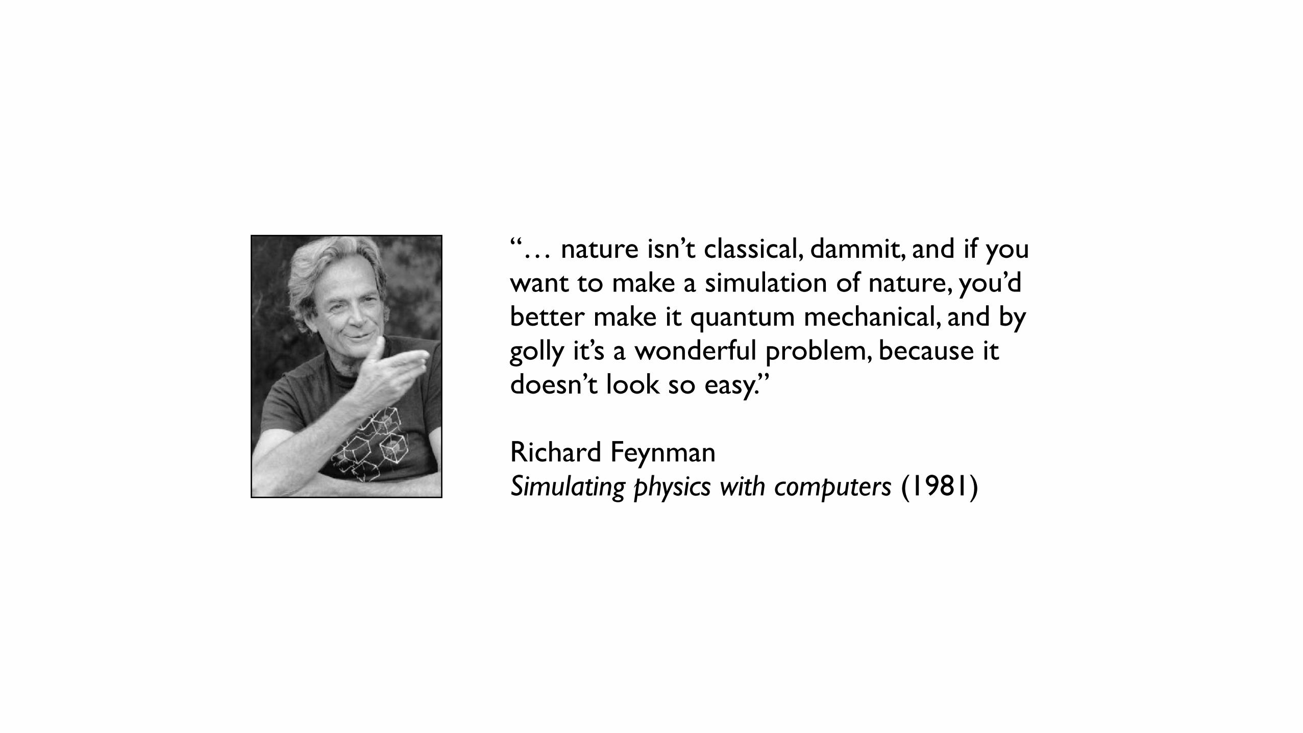
“… nature isn’t classical, dammit, and if you want to make a simulation of nature, you’d better make it quantum mechanical, and by golly it’s a wonderful problem, because it doesn’t look so easy.”

Richard FeynmanSimulating physics with computers (1981)

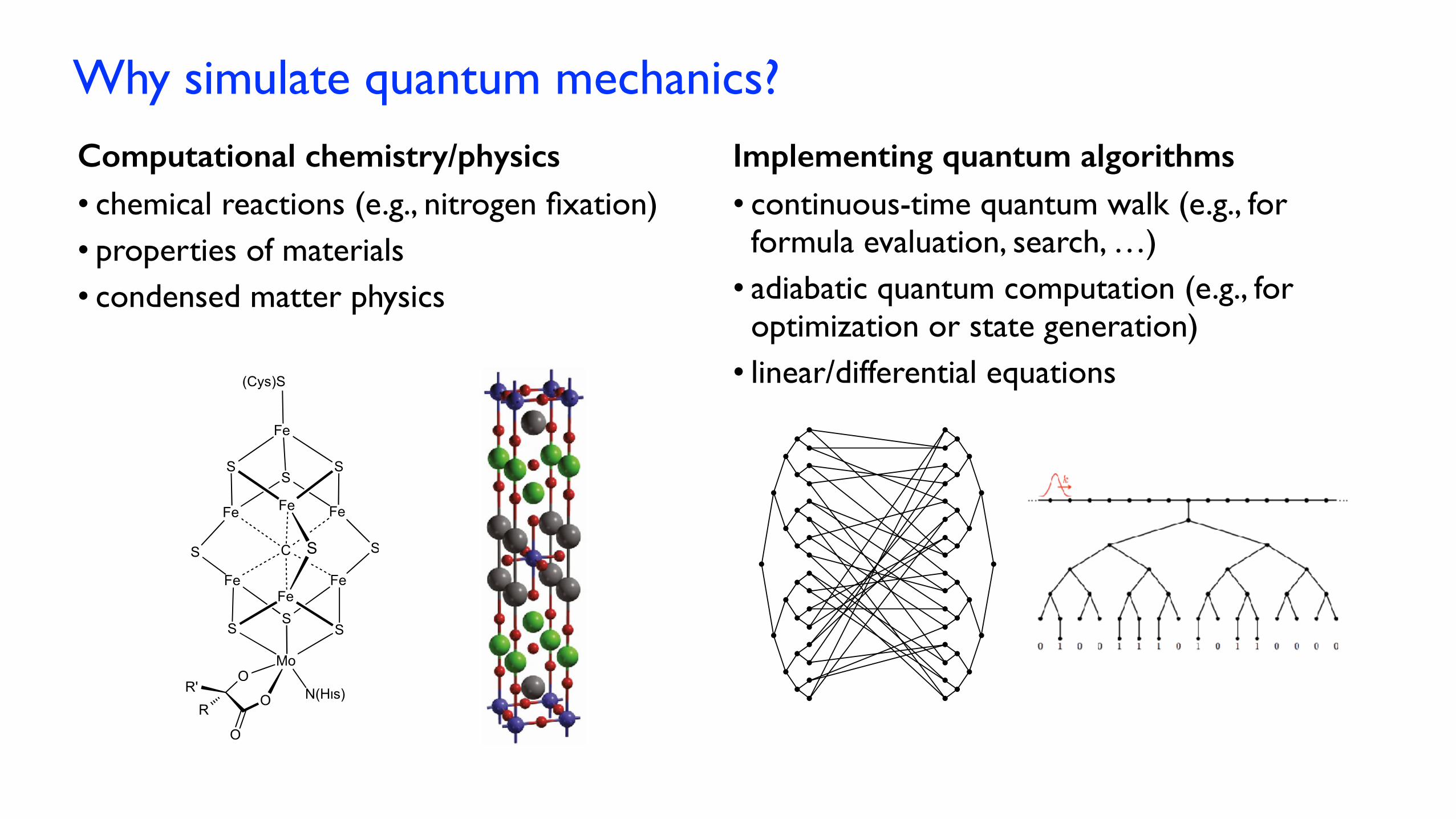
Why simulate quantum mechanics?

Computational chemistry/physics • chemical reactions (e.g., nitrogen fixation)• properties of materials• condensed matter physics

Implementing quantum algorithms • continuous-time quantum walk (e.g., for formula evaluation, search, …)

• adiabatic quantum computation (e.g., for optimization or state generation)

• linear/differential equations

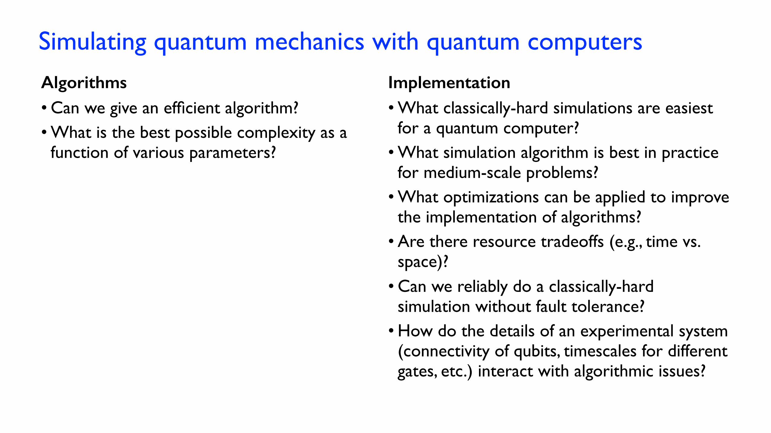
Simulating quantum mechanics with quantum computers

Implementation • What classically-hard simulations are easiest for a quantum computer?

• What simulation algorithm is best in practice for medium-scale problems?

• What optimizations can be applied to improve the implementation of algorithms?

• Are there resource tradeoffs (e.g., time vs. space)?

• Can we reliably do a classically-hard simulation without fault tolerance?

• How do the details of an experimental system (connectivity of qubits, timescales for different gates, etc.) interact with algorithmic issues?

Algorithms • Can we give an efficient algorithm?• What is the best possible complexity as a function of various parameters?

Algorithms

Quantum dynamics

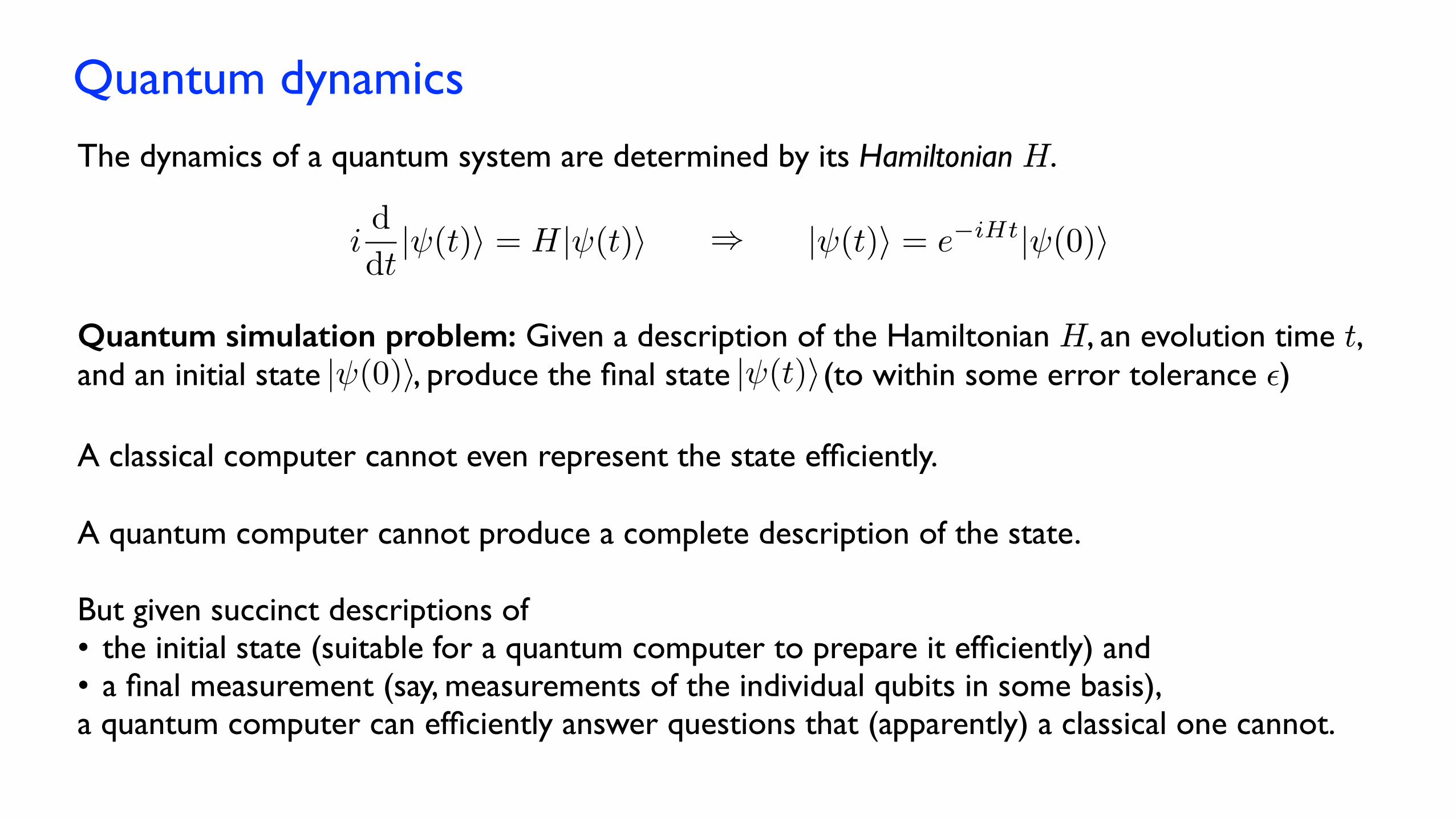
The dynamics of a quantum system are determined by its Hamiltonian H.

A classical computer cannot even represent the state efficiently.

A quantum computer cannot produce a complete description of the state.

id

dt| (t)i = H| (t)i | (t)i = e�iHt| (0)i)

Quantum simulation problem: Given a description of the Hamiltonian H, an evolution time t, and an initial state , produce the final state (to within some error tolerance ²)| (0)i | (t)i

But given succinct descriptions of• the initial state (suitable for a quantum computer to prepare it efficiently) and• a final measurement (say, measurements of the individual qubits in some basis),a quantum computer can efficiently answer questions that (apparently) a classical one cannot.

Local and sparse Hamiltonians

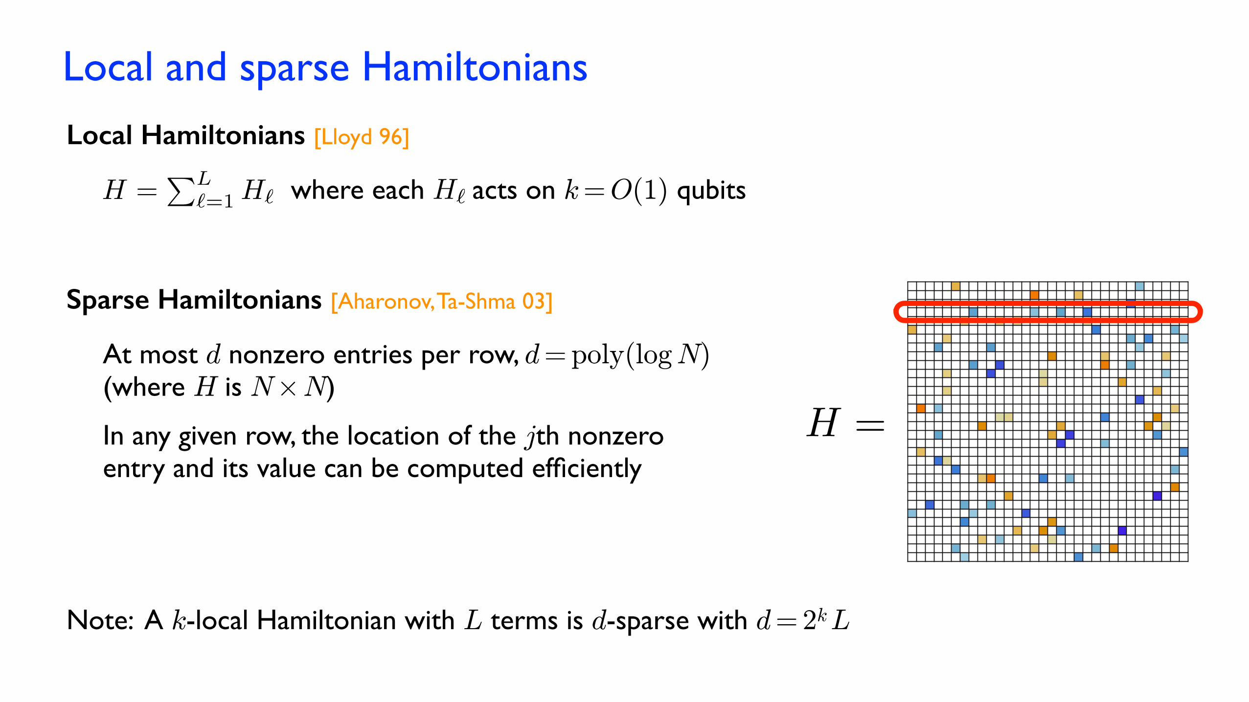
Note: A k-local Hamiltonian with L terms is d-sparse with d = 2k L

Local Hamiltonians [Lloyd 96]

Sparse Hamiltonians [Aharonov, Ta-Shma 03]

At most d nonzero entries per row, d = poly(log N) (where H is N £ N)

H =In any given row, the location of the jth nonzero entry and its value can be computed efficiently

where each acts on k = O(1) qubitsH =PL

`=1 H` H`

Product formula simulation

[Lloyd 96]

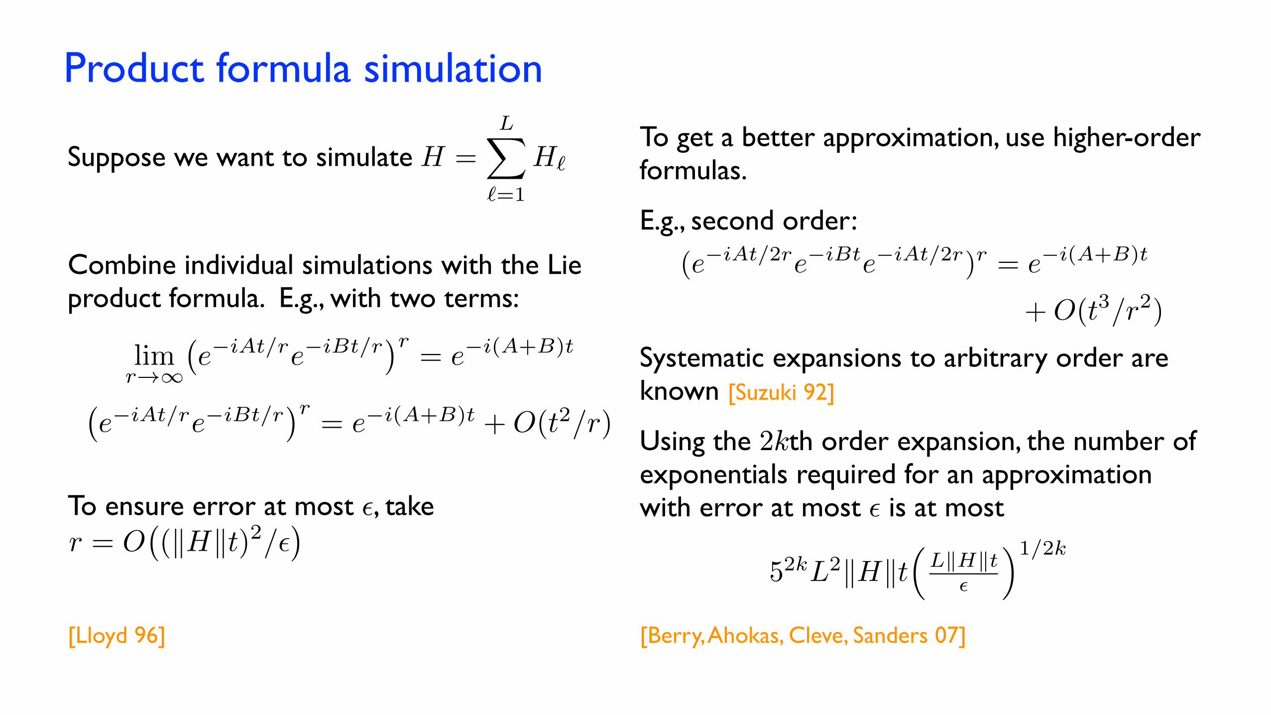
�e�iAt/re�iBt/r

�r= e�i(A+B)t +O(t2/r)

Combine individual simulations with the Lie product formula. E.g., with two terms:

limr!1

�e�iAt/re�iBt/r

�r= e�i(A+B)t

To ensure error at most ², take r = O

�(kHkt)2/✏

�

To get a better approximation, use higher-order formulas.

[Berry, Ahokas, Cleve, Sanders 07]

E.g., second order:

(e�iAt/2re�iBte�iAt/2r)r = e�i(A+B)t

+O(t3/r2)

Suppose we want to simulate H =LX

`=1

H`

Systematic expansions to arbitrary order are known [Suzuki 92]

Using the 2kth order expansion, the number of exponentials required for an approximation with error at most ² is at most

52kL2kHkt⇣

LkHkt✏

⌘1/2k

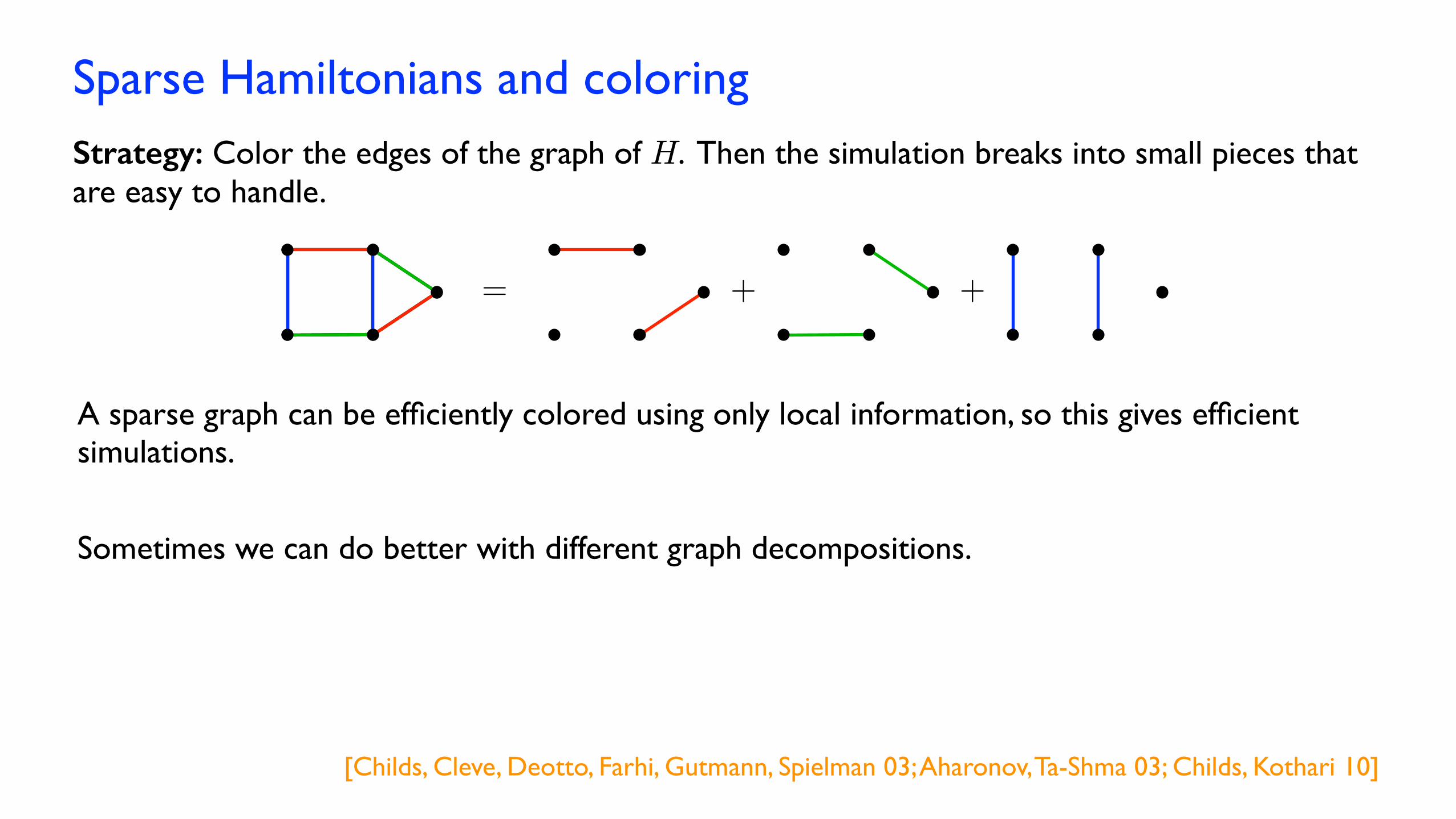
Sparse Hamiltonians and coloringStrategy: Color the edges of the graph of H. Then the simulation breaks into small pieces that are easy to handle.

= + +

[Childs, Cleve, Deotto, Farhi, Gutmann, Spielman 03; Aharonov, Ta-Shma 03; Childs, Kothari 10]

A sparse graph can be efficiently colored using only local information, so this gives efficient simulations.

Sometimes we can do better with different graph decompositions.

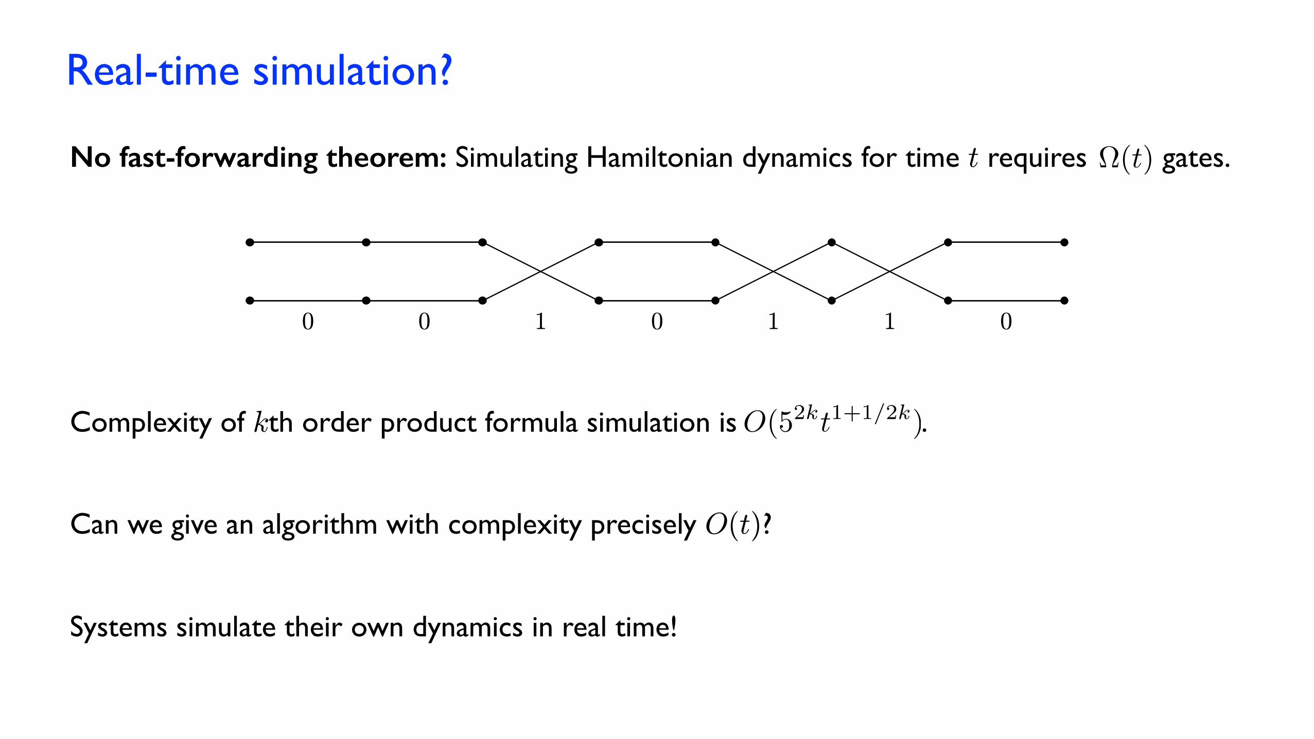
Real-time simulation?

0 0 1 0 1 1 0

Systems simulate their own dynamics in real time!

Can we give an algorithm with complexity precisely O(t)?

No fast-forwarding theorem: Simulating Hamiltonian dynamics for time t requires gates.⌦(t)

Complexity of kth order product formula simulation is .O(52kt1+1/2k)

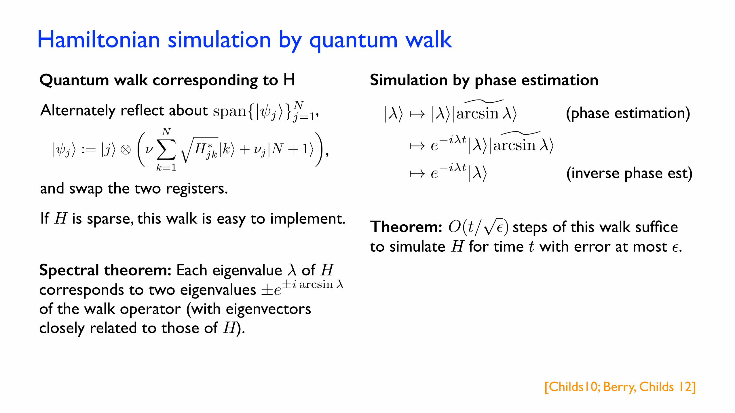
Hamiltonian simulation by quantum walk

[Childs10; Berry, Childs 12]

Spectral theorem: Each eigenvalue ¸ of H corresponds to two eigenvaluesof the walk operator (with eigenvectors closely related to those of H).

±e±i arcsin�

Quantum walk corresponding to H

span{| ji}Nj=1Alternately reflect about ,

| ji := |ji ⌦✓⌫

NX

k=1

qH⇤

jk|ki+ ⌫j |N + 1i◆

and swap the two registers.

,

Simulation by phase estimation

|�i 7! |�i| ^arcsin�i

7! e�i�t|�i| ^arcsin�i7! e�i�t|�i

(phase estimation)

(inverse phase est)

If H is sparse, this walk is easy to implement. Theorem: steps of this walk suffice to simulate H for time t with error at most ².

O(t/p✏)

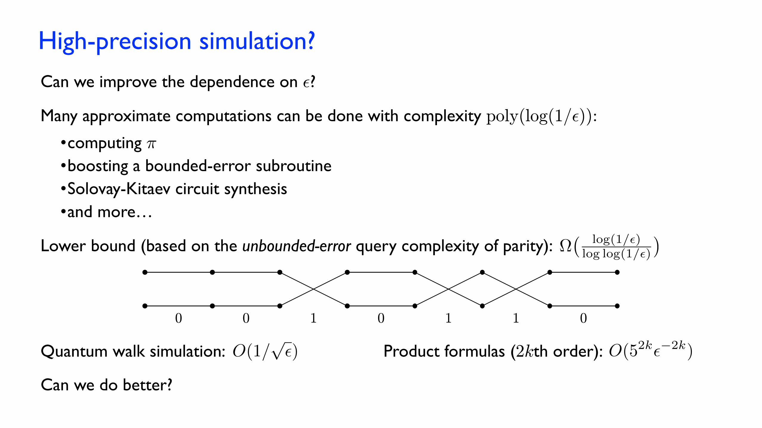
High-precision simulation?

Can we improve the dependence on ²?

Many approximate computations can be done with complexity poly(log(1/²)):

•computing ¼ •boosting a bounded-error subroutine•Solovay-Kitaev circuit synthesis•and more…

Quantum walk simulation: O(1/p✏)

Can we do better?

Product formulas (2kth order): O(52k✏�2k)

Lower bound (based on the unbounded-error query complexity of parity): ⌦�

log(1/✏)log log(1/✏)

�

0 0 1 0 1 1 0

Hamiltonian simulation by linear combinations of unitaries

[Berry, Childs, Cleve, Kothari, Somma 14 & 15]

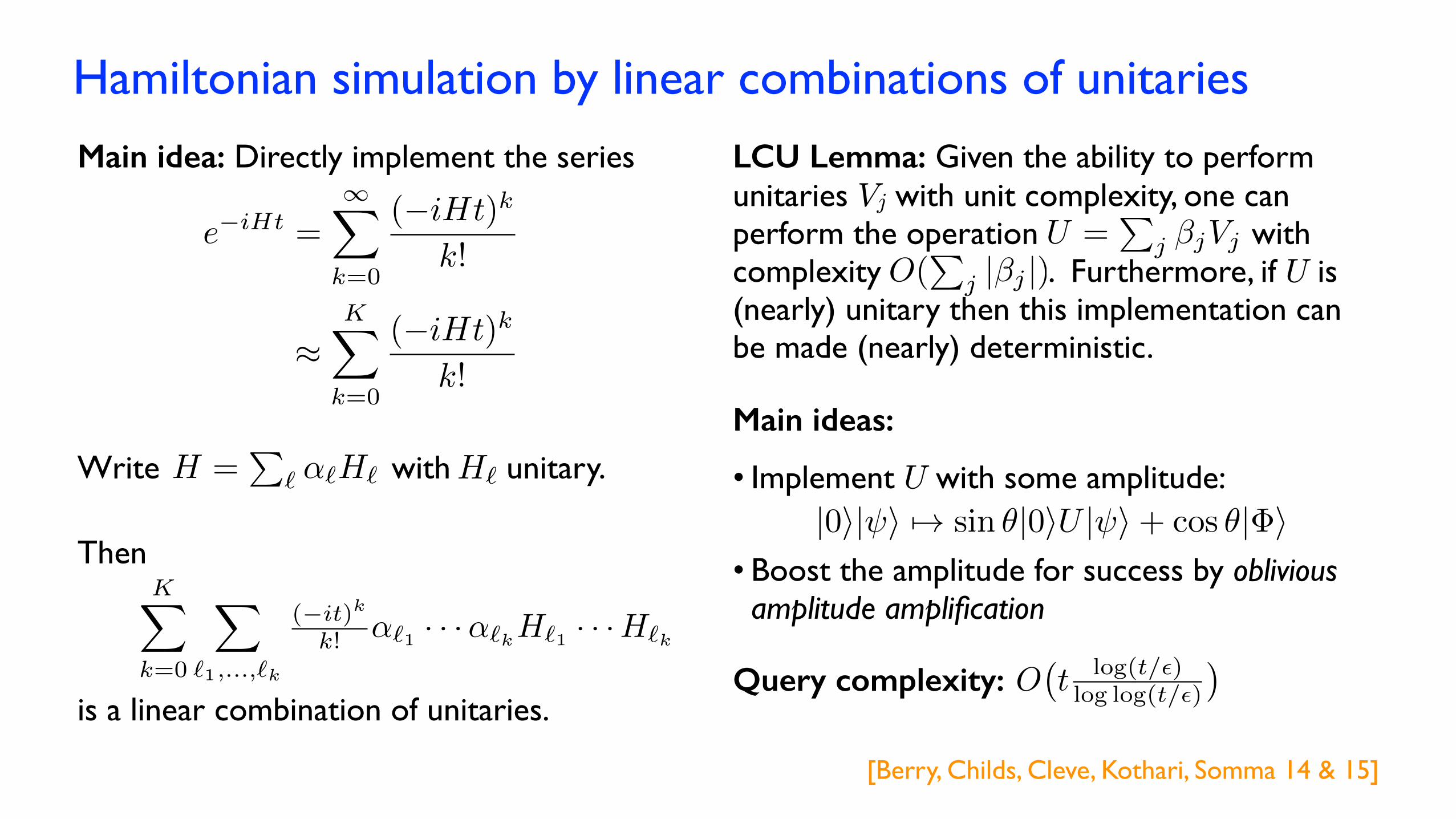
e�iHt =1X

k=0

(�iHt)k

k!

⇡KX

k=0

(�iHt)k

k!

Write with unitary.H =P

` ↵`H` H`

LCU Lemma: Given the ability to perform unitaries Vj with unit complexity, one can perform the operation with complexity . Furthermore, if U is (nearly) unitary then this implementation can be made (nearly) deterministic.

U =P

j �jVj

O(P

j |�j |)

Main idea: Directly implement the series

Then

is a linear combination of unitaries.

KX

k=0

X

`1,...,`k

(�it)k

k! ↵`1 · · ·↵`kH`1 · · ·H`k

Query complexity: O�t log(t/✏)log log(t/✏)

�

Main ideas:

• Boost the amplitude for success by oblivious amplitude amplification

|0i| i 7! sin ✓|0iU | i+ cos ✓|�i• Implement U with some amplitude:

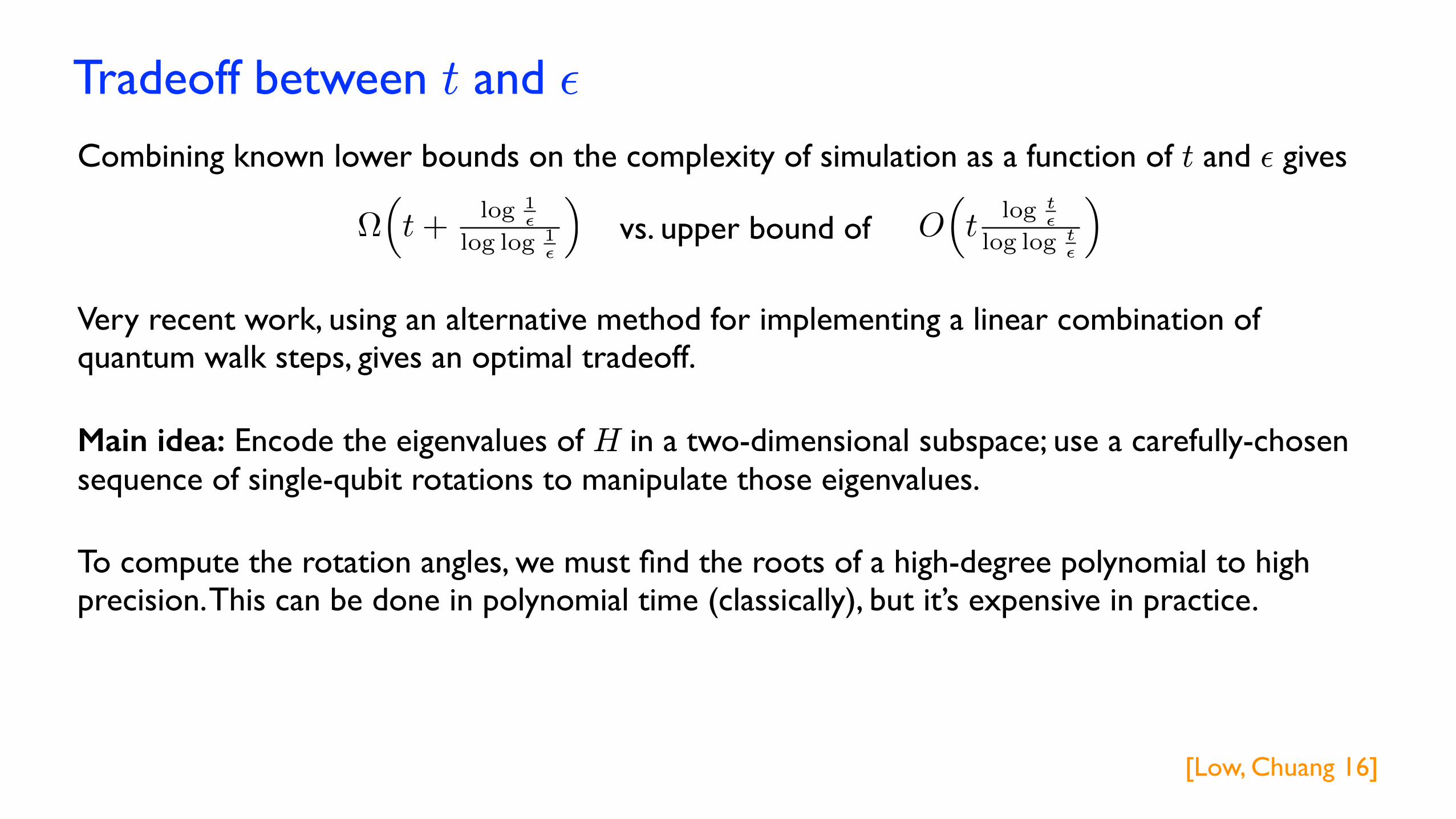
Tradeoff between t and ²

Combining known lower bounds on the complexity of simulation as a function of t and ² gives

⌦⇣t+

log

1✏

log log

1✏

⌘O⇣t

log

t✏

log log

t✏

⌘vs. upper bound of

Very recent work, using an alternative method for implementing a linear combination of quantum walk steps, gives an optimal tradeoff.

[Low, Chuang 16]

Main idea: Encode the eigenvalues of H in a two-dimensional subspace; use a carefully-chosen sequence of single-qubit rotations to manipulate those eigenvalues.

To compute the rotation angles, we must find the roots of a high-degree polynomial to high precision. This can be done in polynomial time (classically), but it’s expensive in practice.

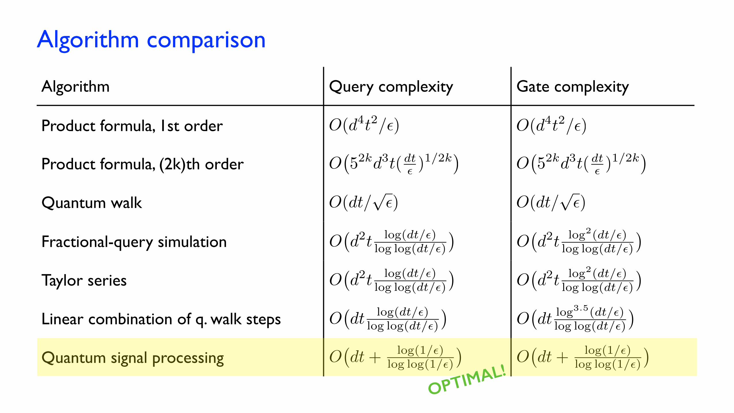
Algorithm comparison

Algorithm Query complexity Gate complexity

Product formula, 1st order

Product formula, (2k)th order

Quantum walk

Fractional-query simulation

Taylor series

Linear combination of q. walk steps

Quantum signal processing

O�d2t log(dt/✏)

log log(dt/✏)

�O�d2t log

2(dt/✏)

log log(dt/✏)

�

O(d4t2/✏) O(d4t2/✏)

O�52kd3t(dt✏ )

1/2k�

O�52kd3t(dt✏ )

1/2k�

O�d2t log(dt/✏)

log log(dt/✏)

�O�d2t log

2(dt/✏)

log log(dt/✏)

�

O(dt/p✏)

O�dt log

3.5(dt/✏)

log log(dt/✏)

�

O(dt/p✏)

O�dt+ log(1/✏)

log log(1/✏)

�O�dt+ log(1/✏)

log log(1/✏)

�O�dt log(dt/✏)

log log(dt/✏)

�

OPTIMAL!

Implementation

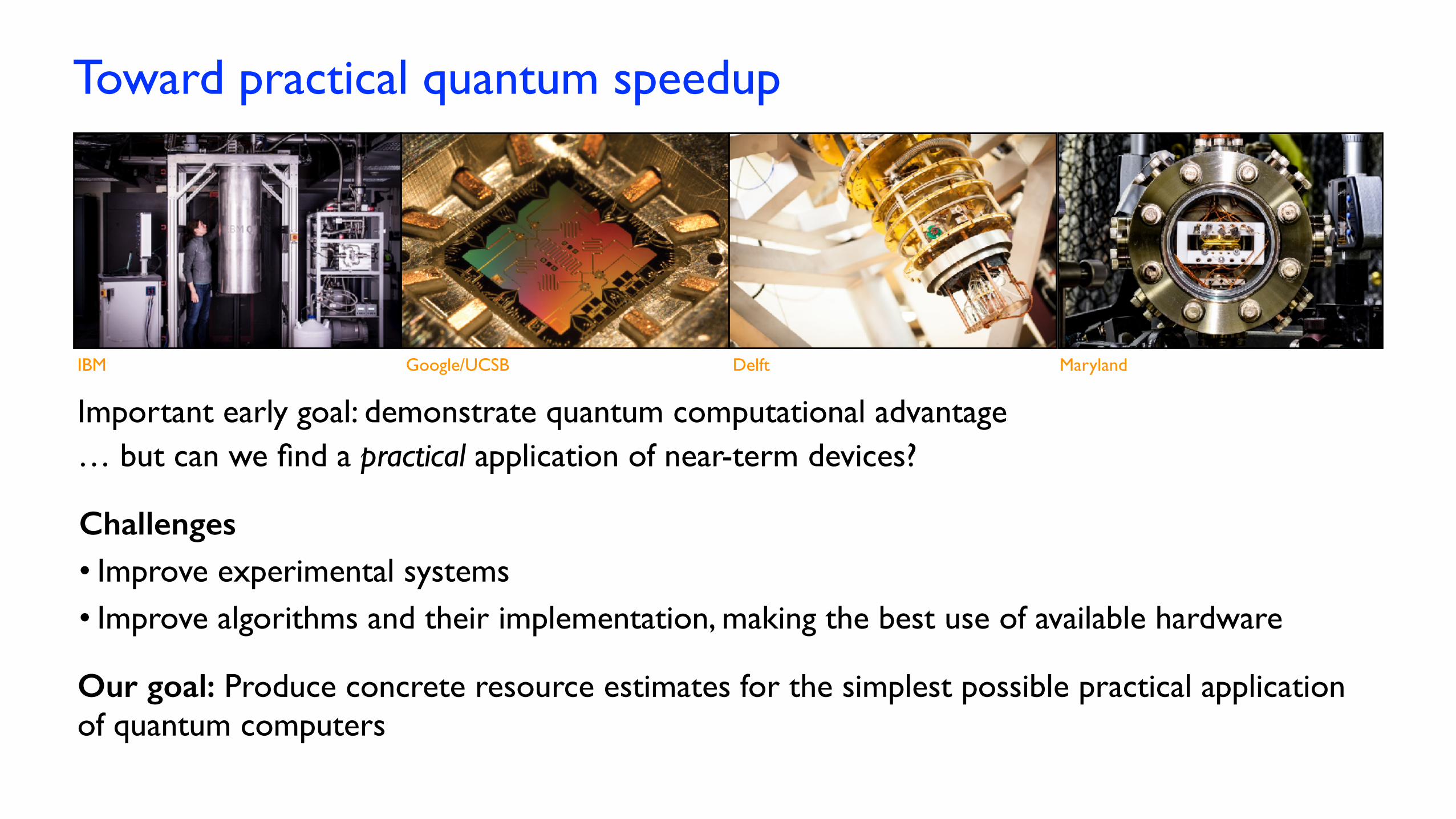
Toward practical quantum speedup

IBM Google/UCSB MarylandDelft

Important early goal: demonstrate quantum computational advantage… but can we find a practical application of near-term devices?

Challenges • Improve experimental systems• Improve algorithms and their implementation, making the best use of available hardware

Our goal: Produce concrete resource estimates for the simplest possible practical application of quantum computers

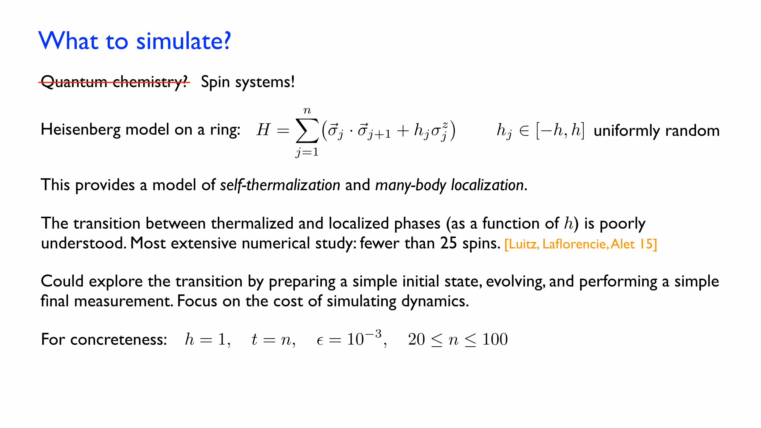
What to simulate?

Quantum chemistry? Spin systems!

Heisenberg model on a ring: H =nX

j=1

�~�j · ~�j+1 + hj�

zj

�hj 2 [�h, h] uniformly random

This provides a model of self-thermalization and many-body localization.

The transition between thermalized and localized phases (as a function of h) is poorly understood. Most extensive numerical study: fewer than 25 spins. [Luitz, Laflorencie, Alet 15]

Could explore the transition by preparing a simple initial state, evolving, and performing a simple final measurement. Focus on the cost of simulating dynamics.

For concreteness: h = 1, t = n, ✏ = 10�3, 20 n 100

Algorithms

Algorithm Gate complexity (t, ²) Gate complexity (n)

Product formula (PF), 1st order

Product formula (PF), (2k)th order

Quantum walk

Fractional-query simulation

Taylor series (TS)

Linear combination of q. walk steps

Quantum signal processing (QSP)

Segmented QSP, q iterates per segment

O(t2/✏)

O(52kt1+1/2k/✏1/2k)

O(t/p✏)

O(n5)

O(52kn3+1/k)

O(n4log n)

O�t log

2(t/✏)

log log(t/✏)

�O�n4

log

2 nlog logn

�

O�t log

2(t/✏)

log log(t/✏)

�O�n3

log

2 nlog logn

�

O�t log

3.5(t/✏)

log log(t/✏)

�O�n4

log

2 nlog logn

�

O(t+ log(1/✏)) O(n3)

O(t1+2/q/✏2/q) O�n3+4/q

�

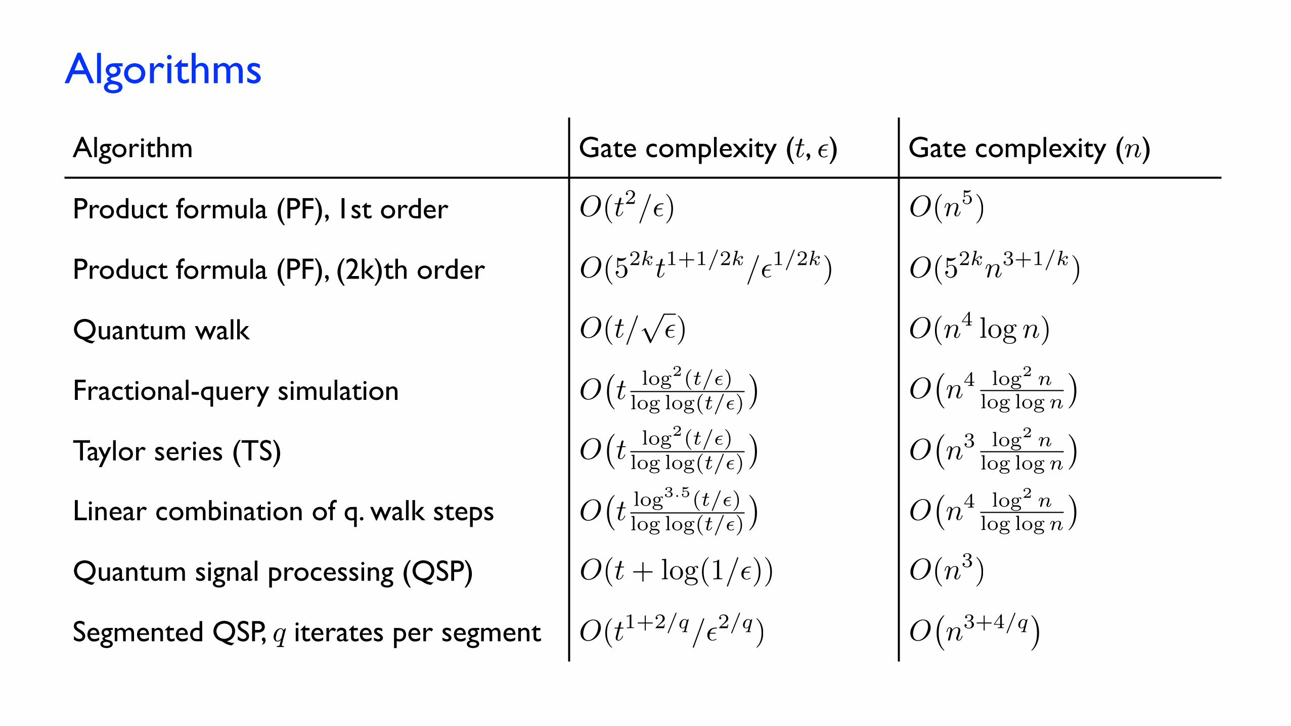
Algorithms

Algorithm Gate complexity (t, ²) Gate complexity (n)

Product formula (PF), 1st order

Product formula (PF), (2k)th order

Quantum walk

Fractional-query simulation

Taylor series (TS)

Linear combination of q. walk steps

Quantum signal processing (QSP)

Segmented QSP, q iterates per segment

O(t2/✏)

O(52kt1+1/2k/✏1/2k)

O(t/p✏)

O(n5)

O(52kn3+1/k)

O(n4log n)

O�t log

2(t/✏)

log log(t/✏)

�O�n4

log

2 nlog logn

�

O�t log

2(t/✏)

log log(t/✏)

�O�n3

log

2 nlog logn

�

O�t log

3.5(t/✏)

log log(t/✏)

�O�n4

log

2 nlog logn

�

O(t+ log(1/✏)) O(n3)

O(t1+2/q/✏2/q) O�n3+4/q

�

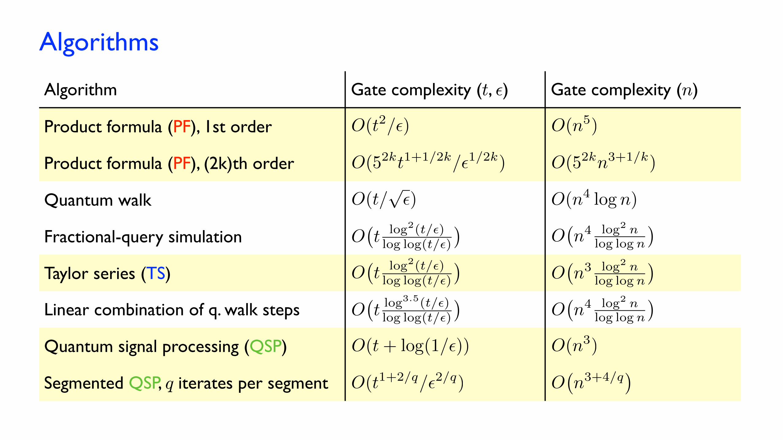
Circuit synthesismultiplexor :: [Double] -> [Qubit] -> Qubit -> Circ ([Qubit], Qubit)multiplexor as controls target = case controls of -- No controls. [] -> do let angle = as !! 0 expYt (- angle) target return ([], target) -- One control. [q0] -> do let (as0, as1) = split_angles as ([], target) <- multiplexor as0 [] target target <- qnot target `controlled` q0 ([], target) <- multiplexor as1 [] target target <- qnot target `controlled` q0 return ([q0], target) -- Two controls. [q0,q1] -> do let (as0, as1) = split_angles as ([q1], target) <- multiplexor as0 [q1] target target <- qnot target `controlled` q0 ([q1], target) <- multiplexor as1 [q1] target target <- qnot target `controlled` q0 return ([q0,q1], target)

-- Three controls. [q0,q1,q2] -> do let (as0, as1, as2, as3) = split_angles_3 as ([q2], target) <- multiplexor as0 [q2] target target <- qnot target `controlled` q1 ([q2], target) <- multiplexor as1 [q2] target target <- qnot target `controlled` q0 ([q2], target) <- multiplexor as3 [q2] target target <- qnot target `controlled` q1 ([q2], target) <- multiplexor as2 [q2] target target <- qnot target `controlled` q0 return ([q0,q1,q2], target)

-- Four or more controls. qs -> do let (as0, as1) = split_angles as let (qhead:qtail) = qs (qtail, target) <- multiplexor as0 qtail target target <- qnot target `controlled` qhead (qtail, target) <- multiplexor as1 qtail target target <- qnot target `controlled` qhead return (qs, target)

where -- Compute angles for recursive decomposition of a multiplexor. split_angles :: [Double] -> ([Double], [Double]) split_angles l = let (l1, l2) = splitIn2 l in let p w x = (w + x) / 2 in let m w x = (w - x) / 2 in (zipWith p l1 l2, zipWith m l1 l2)

-- Compute the angles for recursive decomposition of a multiplexor -- with three controls, saving 2 CNOT gates, as in the -- optimization in Fig. 2 of Shende et.al. split_angles_3 :: [Double] -> ([Double],[Double],[Double],[Double]) split_angles_3 l = let (l1, l2, l3, l4) = splitIn4 l in let pp w x y z = (w + x + y + z) / 4 in let pm w x y z = (w + x - y - z) / 4 in let mp w x y z = (w - x - y + z) / 4 in let mm w x y z = (w - x + y - z) / 4 in let lpp = zipWith4 pp l1 l2 l3 l4 in let lpm = zipWith4 pm l1 l2 l3 l4 in let lmp = zipWith4 mp l1 l2 l3 l4 in let lmm = zipWith4 mm l1 l2 l3 l4 in (lpp, lmm, lpm, lmp)

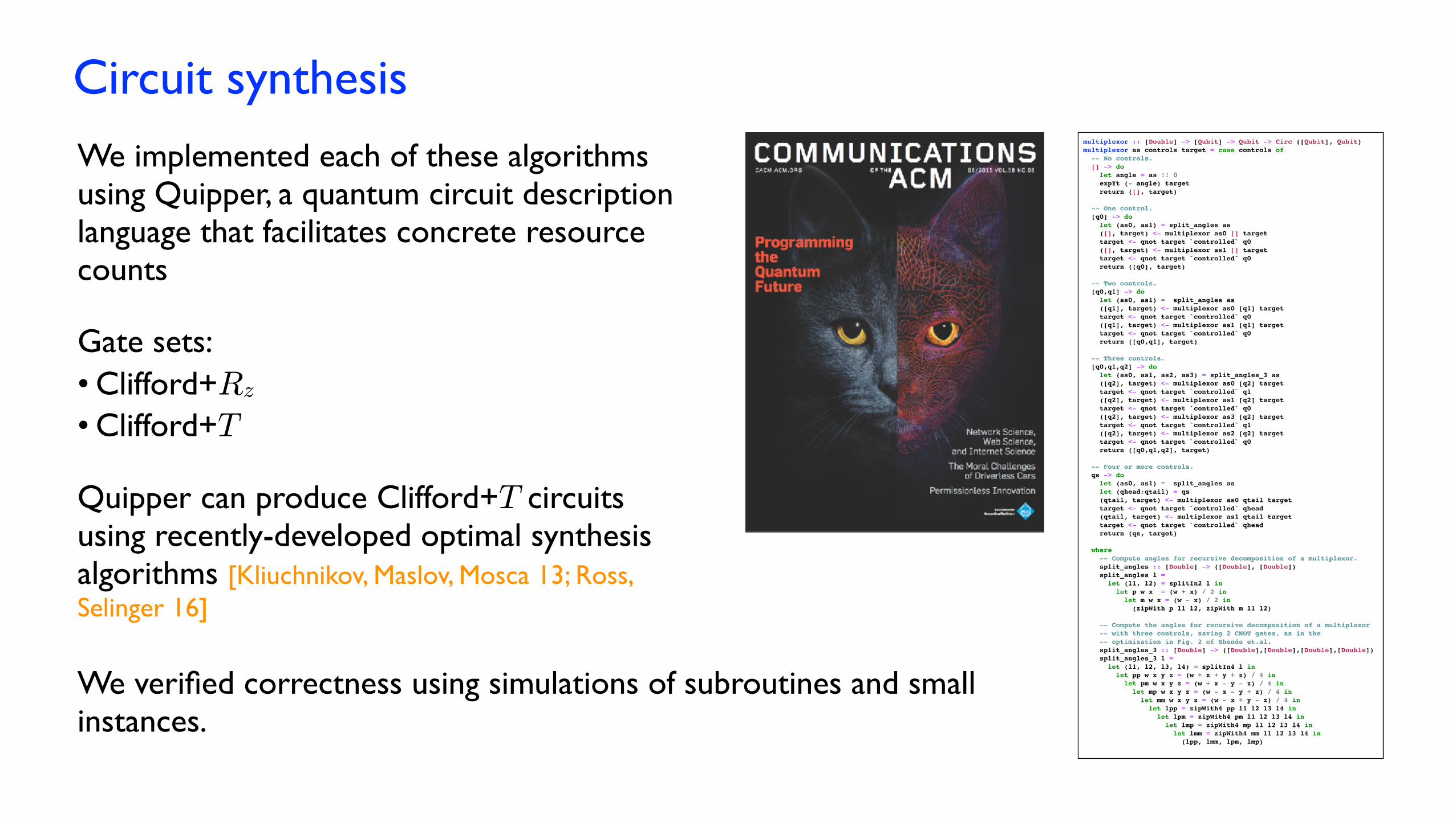
We implemented each of these algorithms using Quipper, a quantum circuit description language that facilitates concrete resource counts

Gate sets:• Clifford+Rz

• Clifford+T

Quipper can produce Clifford+T circuits using recently-developed optimal synthesis algorithms [Kliuchnikov, Maslov, Mosca 13; Ross, Selinger 16]

We verified correctness using simulations of subroutines and small instances.

q0

q1

q2

q3

q4

*

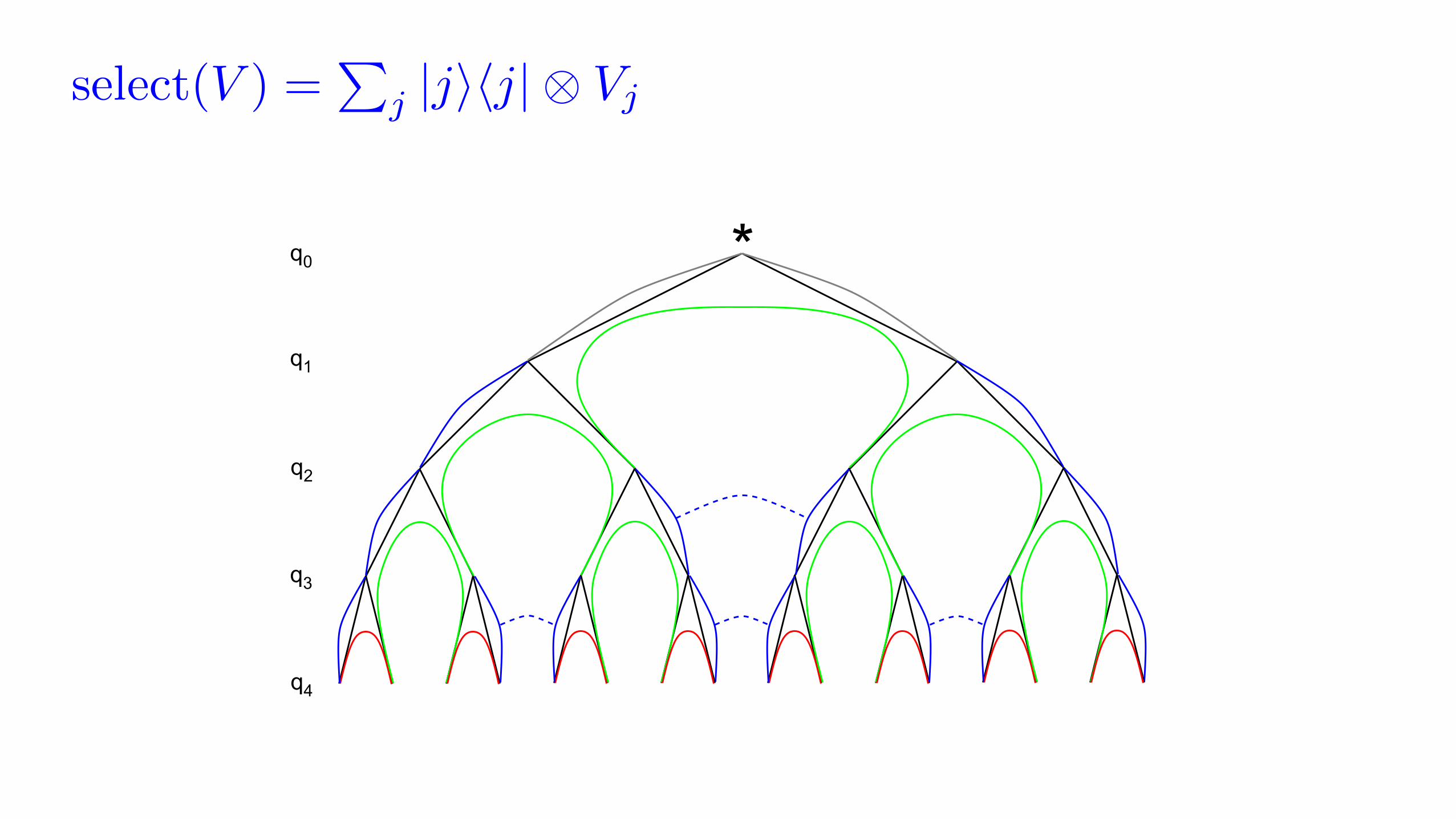
select(V ) =P

j |jihj|⌦ Vj

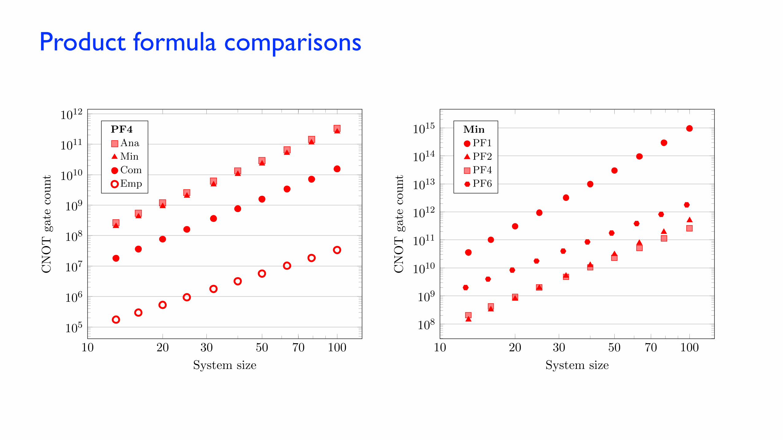
Product formula comparisons

10 100

105

106

107

108

109

1010

1011

1012

20 30 50 70

System size

CNOT

gate

count

PF4Ana

Min

Com

Emp

10 100

108

109

1010

1011

1012

1013

1014

1015

20 30 50 70

System size

CNOT

gate

count

MinPF1PF2PF4PF6

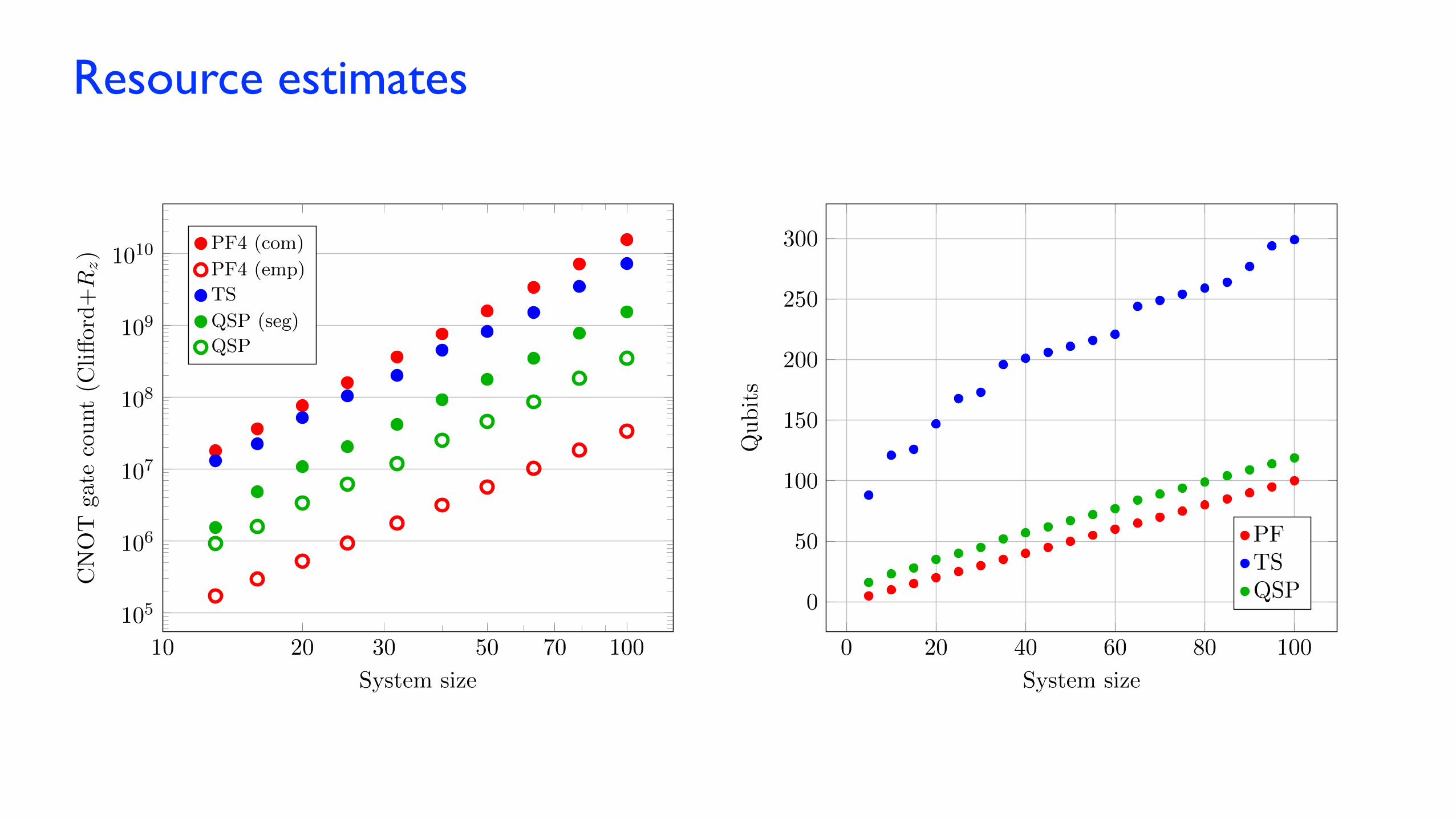
Resource estimates

0 20 40 60 80 100

0

50

100

150

200

250

300

System size

Qubits

PFTSQSP

10 100

105

106

107

108

109

1010

20 30 50 70

System size

CNOT

gate

count(C

li↵ord+R

z) PF4 (com)

TS

QSP (seg)

10 100

105

106

107

108

109

1010

20 30 50 70

System size

CNOT

gate

count(C

li↵ord+R

z) PF4 (com)

PF4 (emp)

TS

QSP (seg)

QSP

Resource estimates

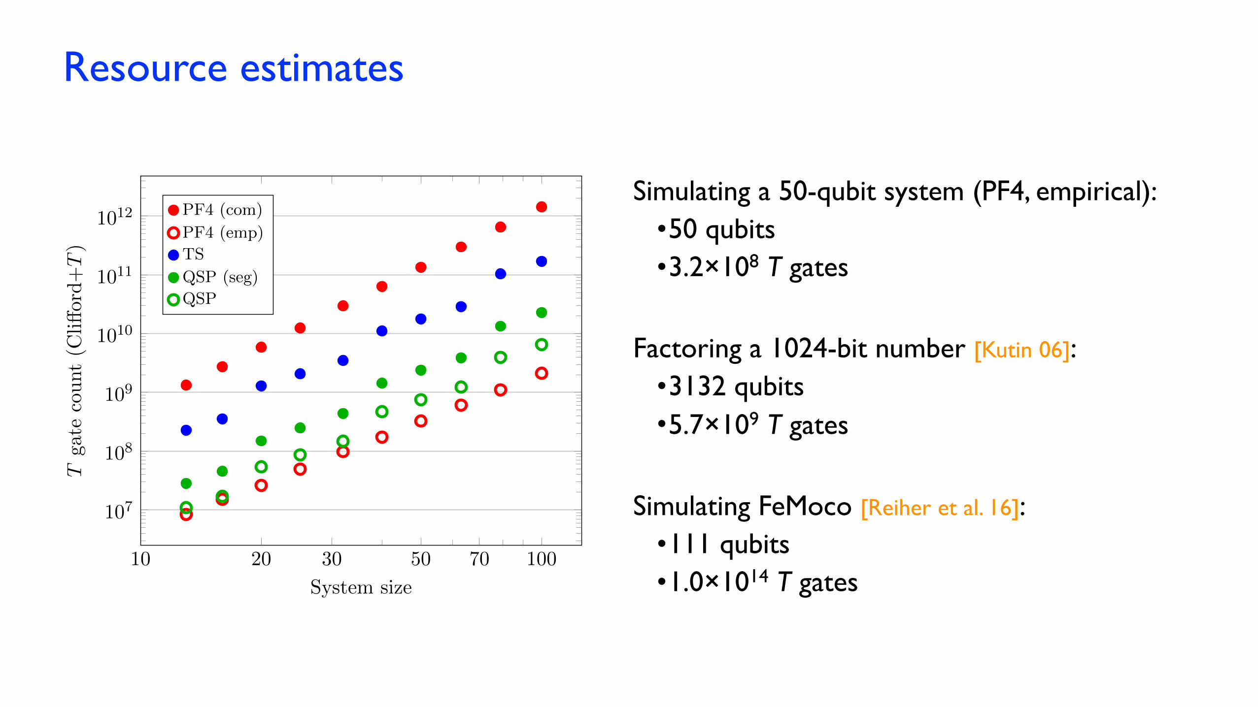
Simulating a 50-qubit system (PF4, empirical):•50 qubits•3.2×108 T gates

Factoring a 1024-bit number [Kutin 06]:•3132 qubits•5.7×109 T gates

Simulating FeMoco [Reiher et al. 16]:•111 qubits•1.0×1014 T gates

10 100

10

7

10

8

10

9

10

10

10

11

10

12

20 30 50 70

System size

Tgatecount(Cli↵ord+T)

PF4 (com)

PF4 (emp)

TS

QSP (seg)

QSP

Outlook

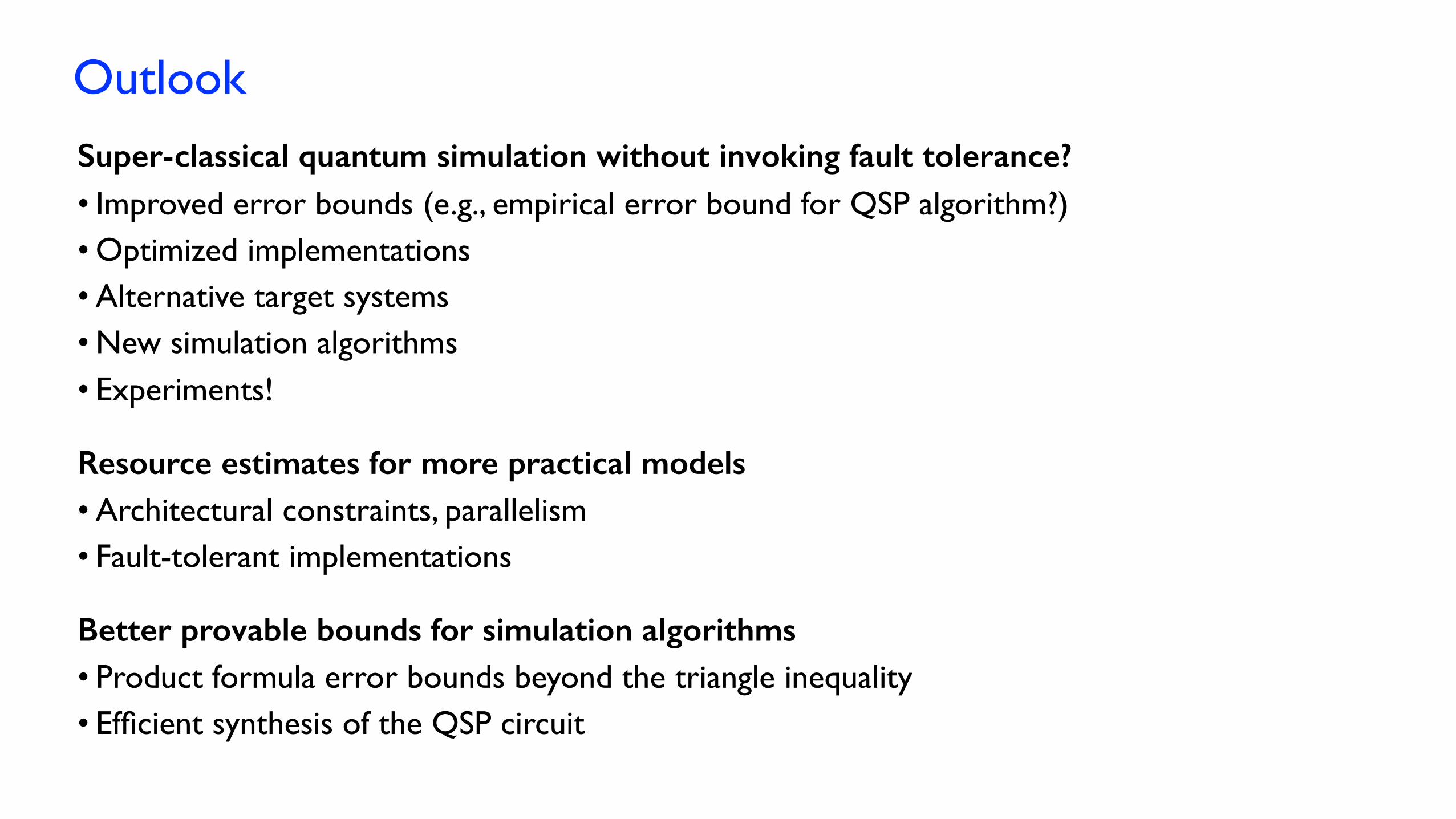
Super-classical quantum simulation without invoking fault tolerance? • Improved error bounds (e.g., empirical error bound for QSP algorithm?)• Optimized implementations• Alternative target systems• New simulation algorithms• Experiments!

Better provable bounds for simulation algorithms • Product formula error bounds beyond the triangle inequality• Efficient synthesis of the QSP circuit

Resource estimates for more practical models • Architectural constraints, parallelism• Fault-tolerant implementations

Algorithms

Dominic Berry Richard Cleve Robin Kothari Rolando Somma

Dmitri Maslov Yunseong Nam Neil Julien Ross Yuan Su

Implementation

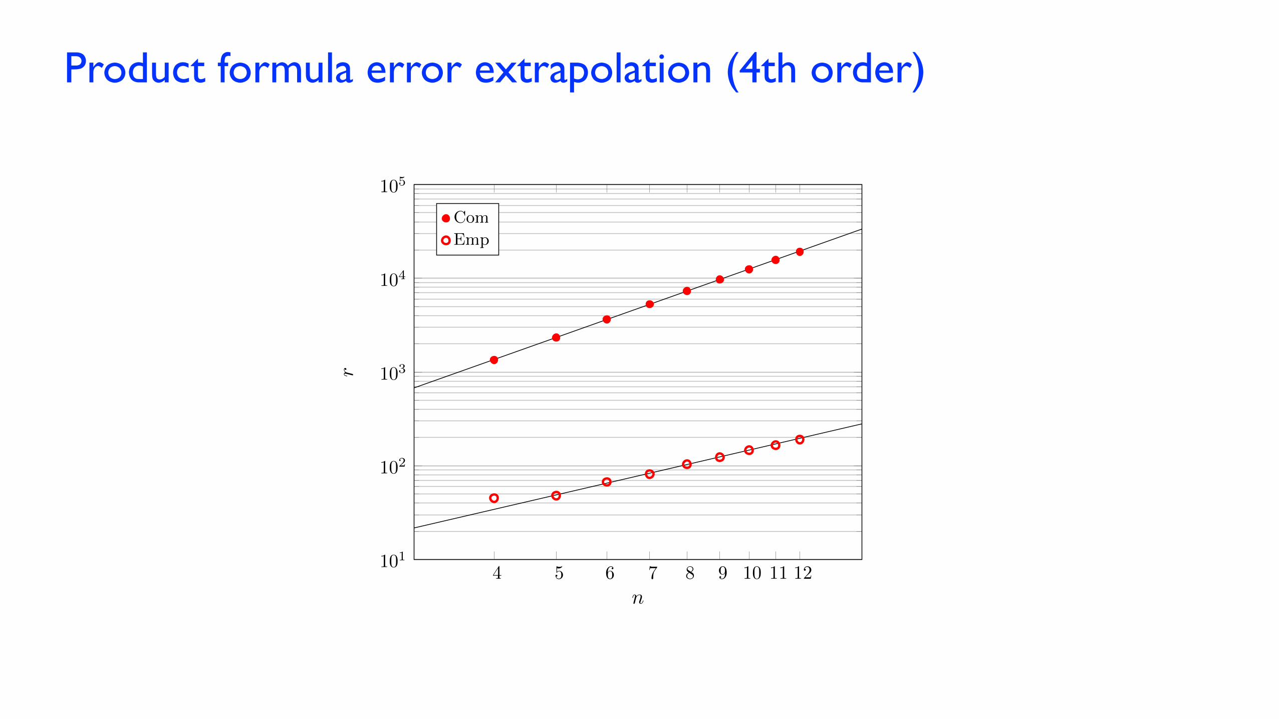
Product formula error extrapolation (4th order)

4 5 6 7 8 9 10 11 12101

102

103

104

105

n

r

Com

Emp