simulating quantum systems on classical computers with
TRANSCRIPT

Simulating Quantum Systems on
Classical Computers with
Matrix Product States
Von der Fakultat fur Mathematik, Informatik undNaturwissenschaften der RWTH Aachen University
zur Erlangung des akademischen Grades eines Doktorsder Naturwissenschaften genehmigte Dissertation
vorgelegt von
Diplom - Physiker
Adrian Kleine
aus Aachen
Berichter: Universitatsprofessor Dr. Ulrich Schollwock
Universitatsprofessorin Dr. Sabine Andergassen
Tag der mundlichen Prufung: 8. November 2010
Diese Dissertation ist auf den Internetseiten derHochschulbibliothek online verfugbar


Abstract
In this thesis, the numerical simulation of strongly-interacting many-body quantum-mechanical
systems using matrix product states (MPS) is considered. Compared to classical systems,
quantum many-body systems possess an exponentially enlarged number of degrees of free-
dom, significantly complicating a simulation on a classical computer.
Matrix-Product-States are a novel representation of arbitrary quantum many-body states.
Using quantum information theory, it is possible to show that Matrix-Product-States pro-
vide a polynomial-sized representation of one-dimensional quantum systems, thus allowing
an efficient simulation of one-dimensional quantum system on classical computers. Matrix-
Product-States form the conceptual framework of the density-matrix renormalization group
(DMRG). Based upon this connection, deeper understanding of the density matrix renormal-
ization group can be obtained.
After a general introduction in the first chapter of this thesis, the second chapter deals with
Matrix-Product-States, focusing on the development of fast and stable algorithms. It is
possible to extend the Matrix-Product-States approach to be able to represent arbitrary op-
erators, the so-called Matrix-Product-Operators, which allows a fast and flexible calculation
of arbitrary expectation values. To obtain algorithms to efficiently calculate groundstates,
the density-matrix renormalization group is reformulated using the Matrix-Product-States
framework. Further, time-dependent problems are considered. Two different algorithms are
presented, one based on a Trotter decomposition of the time-evolution operator, the other
one on Krylov subspaces. Finally, the evaluation of dynamical spectral functions is discussed,
and a correction vector-based method is presented.
3

4
In the following chapters, the methods presented in the second chapter, are applied to a
number of different physical problems. The third chapter deals with the existence of chi-
ral phases in isotropic one-dimensional quantum spin systems. A preceding analytical study
based on a mean-field approach indicated the possible existence of those phases in an isotopic
Heisenberg model with a frustrating zig-zag interaction and a magnetic field. In this thesis,
the existence of the chiral phases will be shown numerically by using Matrix-Product-States-
based algorithms.
A key effect of interacting one-dimensional quantum-mechanical many-body systems is the
spin-charge separation. However, up to now only signs of the spin-charge separation have been
observed in experiments. In the fourth chapter, we propose an experiment using ultracold
atomic gases in optical lattices, which allows a well controlled observation of the spin-charge
separation (of different hyperfine states of the ultracold atoms) with current state of the art
experimental techniques. Ultracold atoms in optical lattices are well described by (Bose)-
Hubbard models. In order to support this proposal, we present numerical results for realistic
system parameters.
Matrix-Product-States are an excellent tool for the simulation of one-dimensional quantum
systems, however, they are not well suited for the simulation of higher dimensional systems.
For strongly-correlated systems, for instance cuprates-based high-temperature superconduc-
tors, quantum fluctuations play an essential role. Classical mean-field theories neglect any
kind of fluctuations, thus they are not suitable to describe strongly-correlated systems. The
dynamical mean-field theory (DMFT) fully takes local quantum fluctuations into account
but neglects any kind of spatial fluctuations. The many-body problem on the lattice is
mapped onto an impurity problem, which needs to be solved self-consistently. In the last
chapter of this thesis, Matrix-Product-States-based algorithms are used to solve the impurity
problem of the dynamical mean-field theory. We present results for a Hubbard model on a
one-dimensional lattice and on a Bethe lattice obtained by the dynamical mean-field and
compare them with exact results.

Kurzzusammenfassung
In der vorliegenden Dissertation wird die numerische Simulation von stark-wechselwirkenden
quantenmechanischen Vielteilchensystem mit Matrix-Produkt-Zustanden (MPS) untersucht.
Quantenmechanische Vielteilchensysteme besitzen im Allgemeinen eine im Vergleich zu klas-
sischen Systemen exponentiell vergroßerte Anzahl Freiheitsgrade, was eine Simulation auf
klassischen Computern signifikant erschwert.
Matrix-Produkt-Zustande sind eine neue Darstellung quantenmechanischer Vielteilchen Zustande.
Basierend auf quanteninformationstheoretischen Uberlegungen kann gezeigt werden, dass
Matrix-Produkt-Zustande Grundzustande von eindimensionalen Quantensystemen mit poly-
nomialem Aufwand darstellen konnen, sie ermoglichen daher eine effiziente numerische Simu-
lation von eindimensionalen Quantensystemen auf klassischen Computern. Matrix-Produkt-
Zustande bilden die theoretische Grundlage der Dichte-Matrix Renormalisierungsgruppe (DMRG),
durch die Formulierung mit Matrix-Produkt-Zustanden kann ein vertieftes Verstandnis der
Dichte-Matrix Renormalisierungsgruppe erhalten werden.
Nach einer allgemeinen Einleitung im ersten Kapitel werden im zweiten Kapitel Matrix-
Produkt-Zustande umfassend diskutiert. Ein Fokus wird auf die Entwicklung von effizien-
ten und stabilen Algorithmen zur Manipulation von Matrix-Produkt-Zustanden gelegt. Es
ist moglich, beliebige Operatoren durch Matrix-Produkt-Operatoren darzustellen, welche ei-
ne schnelle Evaluierung von beliebigen Erwartungswerten ermoglichen. Zur effizienten Be-
rechnung von Grundzustanden wird die Dichte-Matrix Renormalisierungsgruppe im Rahmen
von Matrix-Produkt-Zustanden reformuliert. Im Weiteren werden verschiedene Algorithmen
zur Behandlung von zeitabhangigen Problemen, basierend auf einem Krylov-Unterraum-
Verfahren sowie einer Trotterzerlegung des Zeitentwicklungsoperatorexponentials, vorgestellt
und verglichen. Den Abschluss des Kapitels bildet eine Diskussion uber die Berechnung von
dynamischen Spektralfunktionen mit Matrix-Produkt-Zustanden.
5

6
In den folgenden Kapiteln werden die vorgestellten Methoden auf eine Vielzahl physikalischer
Fragestellungen angewendet. Im dritten Kapitel wird die Existenz von langreichweitigen chi-
ralen Phasen in eindimensionalen isotropen Quantenspinsystemen diskutiert. Eine vorherge-
hende analytische Untersuchung mit einer Molekularfeldnaherung deutete die Existenz dieser
Phasen in einem isotropen Heisenbergmodel mit einer frustrierenden Zickzackwechselwirkung
im Magnetfeld an, in der vorliegenden Arbeit wird die Existenz solcher Phasen mittels auf
Matrix-Produkt-Zustanden basierenden Methoden numerisch gezeigt.
Ein wesentlicher Effekt eindimensionaler wechselwirkender quantenmechanischer Vielteil-
chensysteme ist die Spin-Ladungs-Trennung. Mit heutigen experimentellen Methoden ist es
jedoch schwierig die Spin-Ladungs-Trennung experimentell zu beobachten bzw. zu kontrol-
lieren. Ultrakalte Atomgase in optischen Gittern sind hochreine quantenmechanische Viel-
teilchensysteme, bei denen eine hochprazise Kontrolle aller Systemparameter moglich ist. Im
vierten Kapitel wird ein Experiment vorgeschlagen, das mit heutigen experimentellen Techni-
ken eine Spin-Ladungs-Trennung von unterschiedlichen Hyperfeinzustanden eines Atomgases
beobachtbar machen sollte. Um dies zu uberprufen, werden fur realistische Systemparameter
in diesem Kapitel Simulationen durchgefuhrt.
Matrix-Produkt-Zustande sind ein hervorragendes Werkzeug zur Beschreibung von eindimen-
sionalen Systemen, sie sind fur hoherdimensionale Systeme jedoch nicht geeignet. Klassische
Molekularfeldnaherungen vernachlassigen jede Art von Fluktuationen. In stark-korrelierten
Systemen, wie zum Beispiel Hochtemperatursupraleitern (Cuprate), spielen Quantenfluktua-
tionen eine wesentliche Rolle. Die dynamische Molekularfeldnaherung (DMFT) behandelt lo-
kale quantenmechanische Fluktuationen exakt, vernachlassigt aber raumliche Fluktuationen.
Ein quantenmechanisches Vielteilchenproblem auf einem Gitter wird durch die dynamische
Molekularfeldnaherung auf ein selbstkonsistent zu losendes Storstellenproblem abgebildet. Im
letzten Kapitel wird dieses Storstellenproblem der dynamischen Molekularfeldnaherung mit
den im zweiten Kapitel vorgestellten Algorithmen gelost, und Ergebnisse fur ein Hubbard
Modell auf einem Bethe Gitter sowie einem eindimensionalen Hubbard Modell vorgestellt
und mit exakten Ergebnissen verglichen.

Contents
1 Introduction 13
2 Matrix Product States 19
2.1 Introduction . . . . . . . . . . . . . . . . . . . . . . . . . . . . . . . . . . . . . 19
2.2 Matrix Product States . . . . . . . . . . . . . . . . . . . . . . . . . . . . . . . 24
2.2.1 Matrix Product Wavefunctions . . . . . . . . . . . . . . . . . . . . . . 24
2.2.2 Matrix Product Operators . . . . . . . . . . . . . . . . . . . . . . . . . 27
2.2.3 Symmetries . . . . . . . . . . . . . . . . . . . . . . . . . . . . . . . . . 30
2.3 DMRG . . . . . . . . . . . . . . . . . . . . . . . . . . . . . . . . . . . . . . . . 32
2.3.1 Local Optimization . . . . . . . . . . . . . . . . . . . . . . . . . . . . . 32
2.3.2 Truncation . . . . . . . . . . . . . . . . . . . . . . . . . . . . . . . . . 33
2.3.3 Application of the Algorithms . . . . . . . . . . . . . . . . . . . . . . . 35
2.4 Time-Dependent Problems . . . . . . . . . . . . . . . . . . . . . . . . . . . . . 38
2.4.1 Trotter Decomposition . . . . . . . . . . . . . . . . . . . . . . . . . . . 38
2.4.2 Krylov Subspace Methods . . . . . . . . . . . . . . . . . . . . . . . . . 40
2.4.3 Comparison . . . . . . . . . . . . . . . . . . . . . . . . . . . . . . . . . 42
2.5 Frequency Space Algorithms . . . . . . . . . . . . . . . . . . . . . . . . . . . . 46
2.5.1 Introduction . . . . . . . . . . . . . . . . . . . . . . . . . . . . . . . . 46
2.5.2 GMRES . . . . . . . . . . . . . . . . . . . . . . . . . . . . . . . . . . . 47
2.5.3 Analysis . . . . . . . . . . . . . . . . . . . . . . . . . . . . . . . . . . . 48
2.6 Conclusion . . . . . . . . . . . . . . . . . . . . . . . . . . . . . . . . . . . . . 51
7

8 CONTENTS
3 Vector Chiral Order in 1D Spin Chains 53
3.1 Introduction . . . . . . . . . . . . . . . . . . . . . . . . . . . . . . . . . . . . . 53
3.2 Model and Analytical Predictions . . . . . . . . . . . . . . . . . . . . . . . . . 55
3.3 DMRG results . . . . . . . . . . . . . . . . . . . . . . . . . . . . . . . . . . . 59
3.3.1 S = 1 . . . . . . . . . . . . . . . . . . . . . . . . . . . . . . . . . . . . 60
3.3.2 S = 1/2 . . . . . . . . . . . . . . . . . . . . . . . . . . . . . . . . . . . 64
3.4 Conclusions and Outlook . . . . . . . . . . . . . . . . . . . . . . . . . . . . . 65
4 Bosonic Spin Charge Separation 69
4.1 Introduction . . . . . . . . . . . . . . . . . . . . . . . . . . . . . . . . . . . . . 69
4.2 Bose-Hubbard Model . . . . . . . . . . . . . . . . . . . . . . . . . . . . . . . . 73
4.2.1 Single-Component Bose-Hubbard Model . . . . . . . . . . . . . . . . . 73
4.2.2 Two-Component Bose-Hubbard Model . . . . . . . . . . . . . . . . . . 77
4.3 Numerical Results . . . . . . . . . . . . . . . . . . . . . . . . . . . . . . . . . 80
4.3.1 Velocities and Luttinger Parameter . . . . . . . . . . . . . . . . . . . . 80
4.3.2 Single Particle Excitations . . . . . . . . . . . . . . . . . . . . . . . . . 85
4.3.3 Spectral Functions . . . . . . . . . . . . . . . . . . . . . . . . . . . . . 87
4.3.4 Entropy of Entanglement . . . . . . . . . . . . . . . . . . . . . . . . . 89
4.3.5 Experimental Constraints . . . . . . . . . . . . . . . . . . . . . . . . . 90
4.4 Conclusion . . . . . . . . . . . . . . . . . . . . . . . . . . . . . . . . . . . . . 91
5 Dynamical Mean-Field Theory 95
5.1 Introduction . . . . . . . . . . . . . . . . . . . . . . . . . . . . . . . . . . . . . 95
5.2 Dynamical Mean Field Theory . . . . . . . . . . . . . . . . . . . . . . . . . . 97
5.2.1 Derivation of the DMFT Equations . . . . . . . . . . . . . . . . . . . . 97
5.2.2 Solving the DMFT Equation . . . . . . . . . . . . . . . . . . . . . . . 102
5.3 Results . . . . . . . . . . . . . . . . . . . . . . . . . . . . . . . . . . . . . . . . 110
5.3.1 Bethe Lattice . . . . . . . . . . . . . . . . . . . . . . . . . . . . . . . . 110
5.3.2 One-dimensional Hubbard model . . . . . . . . . . . . . . . . . . . . . 115
5.4 Conclusion . . . . . . . . . . . . . . . . . . . . . . . . . . . . . . . . . . . . . 117

CONTENTS 9
A Deconvolution 119
A.1 Introduction . . . . . . . . . . . . . . . . . . . . . . . . . . . . . . . . . . . . . 119
A.2 Methods . . . . . . . . . . . . . . . . . . . . . . . . . . . . . . . . . . . . . . . 122
A.2.1 Linear Schemes . . . . . . . . . . . . . . . . . . . . . . . . . . . . . . . 122
A.2.2 Maximum Entropy Methods . . . . . . . . . . . . . . . . . . . . . . . . 127
A.3 Comparison and Conclusion . . . . . . . . . . . . . . . . . . . . . . . . . . . . 133
Bibliography 137
Publications 144
Curriculum Vitae 146
Acknowledgements 148
Eidesstattliche Erklarung 150

“There is a theory which states that if ever
anyone discovers exactly what the Universe is
for and why it is here, it will instantly disappear
and be replaced by something even more bizarre
and inexplicable.”
Douglas Adams, The Restaurant at the End of the Universe, Hitchhiker’s Guide to the Galaxy

“There is another theory which states that this
has already happened.”
Ibid.


Chapter 1
Introduction
Let us start by considering a simple quantum-mechanical particle. The state of the systemis completely described by the complex-valued wavefunction Ψ(~x1; t) which is a function ofthe spatial coordinate of the particle ~x1 and the time t. All possible states form an infinite-dimensional Hilbert space, H0. However, it is also possible to restrict oneself to a finitenumber of particle orbitals, yielding a Hilbert space with a finite dimension, given by dimH0.
Prominent examples are simple quantum spin models, where one only considers the spindegrees of freedom of a single localized spin. In the case of a spin-1/2 system one obtains atwo-dimensional local Hilbert space spanned by |↑〉 and |↓〉.
What happens when considering N particles? The wavefunction is now a function of allspatial coordinates ~xi, i.e. Ψ(~x1, ~x2, . . . ~xN ; t). The Hilbert space of the many-particle wave-functions, H, can now be written as product space of N single particle Hilbert spaces H0,yielding
H =
N⊗
i=1
H0. (1.1)
It is important to note that the dimension of the Hilbert space scales exponentially in thenumber of particles,
dimH = (dimH0)N
. (1.2)
This scaling is fundamentally different in a classical system. The state of a classical systemwith N particles is given by the 3N -dimensional vector, x(t) = (~x1(t), . . . , ~xN (t)) ∈ R
3N ,thus a linear scaling can be observed.
The inherent complexity of a quantum-mechanical system is both a boon and a bane at thesame time. It can be exploited in a quantum computer, allowing for instance factorization ofan integer by using Shor’s algorithm [5, 6], which is polynominally bounded in time. However,on the other side, the exponential complexity prevents an efficient simulation of an arbitrary
13

14 CHAPTER 1. INTRODUCTION
quantum system on a classical computer, [9].
However, for physical systems whose correlations are weak, one can set up an effective singleparticle description of the problem. The many-particle interactions, like for instance theelectrostatic electro-electron repulsion, are treated on a mean-field level. There are a numberof different methods available, for example the Hartree-Fock method, and the more advanceddensity functional theory (DFT) combined with a local density approximation (LDA) [13–15], to name two important methods. For weakly-correlated systems these methods yieldexcellent results.
This changes when considering strongly-correlated systems. A number of interesting sys-tems like transition metal oxides (for instance NiO, where a Mott-insulating phase can beobserved), or high-temperature superconductors possess strong electronic correlations, hencemethods like LDA or HF are not able to describe these systems.
In general metal-insulator transitions of strongly correlated electronic systems, for instanceof the Hubbard model [7], are of great interest. These systems possess a number of effectswhich can be attributed to the strong correlations present. For instance the high-temperaturesupraconductivity in cuprate compounds [8], is believed to be described by a two-dimensionalunderdoped Hubbard model, but, however, up to now this model eluded all analytical andnumerical attempts.
A simple brute-force solution of the general problem can be obtained by (numerically) di-agonalizing to full Hilbert space H. However, this approach is limited to only small systemsizes, as the occurring matrices scale exponentially with the system size.
Now, the question arouses whether this exponential complexity is inherent to the problem,or whether there are faster algorithms for simulating a quantum-mechanical system possible.I.e. is the full treatment always necessary, or are there efficient algorithms available for sim-ulating specific strongly-correlated systems.
Focusing on the exponential growths of the Hilbert space one may resort to Monte-Carlomethods which tries to sample the full Hilbert space. One randomly draws states xi fromthe Hilbert which contribute to the desired physical state with the probability pi. Theexpectation value of an operator A can now be written as
〈A〉 ≈
N∑
i=1
piA(xi)
N∑
i=1
pi
. (1.3)
However, in general it is not possible to set a Monte-Carlo scheme for a quantum system forwhich pi is always positive. As long as the expectation value of pi is non-zero, i.e.
〈p〉 =1
N
N∑
i=1
pi 6= 0, (1.4)

15
it is still possible to evaluate Eq. 1.3 faithfully. When 〈p〉 becomes small,∣∣ 〈p〉
∣∣ ≪ 1, the
numerical condition of this approach deteriorates, thus introducing (possibly large) errors tothe sums. This effect is known as sign-problem. When the sign-problem is not present, how-ever, Quantum Monte-Carlo methods provide an efficient simulation of strongly-correlatedsystems.
It turns out that for bosonic and spin models, which do not possess any frustrated inter-actions, Quantum Monte-Carlo methods exists, where 〈p〉 stays finite. However, addingfrustrations to the system introduces a sign problem, which becomes arbitrarily strong inthe limit of small temperatures, β → ∞. The sign problem is also present when consideringfermionic systems. In this case, one can show that the sign problem is NP-complete[10], thusa difficult problem to solve.
A different approach uses quantum information theory to determine the relevant parts of theHilbert space to describe a given state. Consider a system in the pure state |Ψ〉, and dividethe system into two parts, subsystem A and B. The density matrices ρA,B for both subsystemscan now be obtained by simply tracing out the other subsystem, i.e. ρA = TrB |Ψ〉 〈Ψ|, andρB = TrA |Ψ〉 〈Ψ|. The entanglement entropy
S = −TrB (ρA log ρA) = −TrA (ρB log ρB) (1.5)
provides a measure of the (quantum) information contained in the entanglement betweenboth subsystems. Schuhmacher’s noiseless channel coding theorem [6] now states that Squbits are needed to represent the information faithfully. This result is the quantum ver-sion of the well-known Shannon’s source coding theorem of the classical information theory,which states that Shannon entropy, S = −∑
i pi log pi, measures how many classical bits areneeded to store the information of a message. In the classical information theory, one cannow use this theorem as starting point to construct efficient quantum compression algorithms.
Consider a system with L sites and the local Hilbert space of site i is spanned by |αi〉. Ageneral state can now be written down,
|Ψ〉 =∑
α1
∑
α2
· · ·∑
αL
Aα1,α2,...αL |α1〉 ⊗ |α2〉 ⊗ . . . ⊗ |αL〉 , (1.6)
where Aα1,α2,...αL is a rank-L tensor. It is always possible to decompose an arbitrary rank-ktensor Aαβ into a product of a rank-(kα + 1), Bγ
α, and a rank-(kβ + 1) tensor Cγβ,
Aαβ = BγαCγ
β. (1.7)
α is a rank-kα superindex, β a rank-kβ one, i.e. k = kα + kβ . Now one can write the tensorAα1,α2,...αL as product of rank-3 tensors,
Aα1,α2,...αL = A1(α1)γ1
A2(α2)γ1γ2
· · · AL−1(αL−1)γL−2γL−1
AL(αL)γL−1
, (1.8)
as sketched in Fig. 1.1. One can split the system into two subsystems by considering oneindex γi; now it can be shown by using the Schmidt decomposition that the entanglement

16 CHAPTER 1. INTRODUCTION
a)
b)
|α1〉
|α1〉
|α2〉
|α2〉
|α3〉
|α3〉
|αL−2〉
|αL−2〉
|αL−1〉
|αL−1〉
|αL〉
|αL〉
Aα1,...,αL
A1 A2 A3 AL−2 AL−1AL
Figure 1.1: A general state of the Hilbert space (a), and the construction of Matrix ProductStates (b).
entropy, Eq. 1.5, provides a measurement of the dimension of this index needed to faithfully
represent the state |Φ〉. Ai(αi)γi−1γi
≡(
Ai(αi)
)
γi−1γi
can be interpreted as matrix with the
additional index αi. Now one can write down a general state,
|Ψ〉 =∑
α1
∑
α2
· · ·∑
αL
A1(α1)A2
(α2) · · ·AL(αL) |α1〉 ⊗ |α2〉 ⊗ . . . ⊗ |αL〉 , (1.9)
using the matrix product. Therefore this representation of the Hilbert space is called matrixproduct states (MPS). These states form the theoretical framework of the density matrixrenormalization group (DMRG) algorithm[11, 12].
In the next chapter, we will discuss matrix product states in great detail, and especiallyconsider a number of algorithms which are able to efficiently handle MPS numerically. Itwill turn out that MPS are only a good ansatz for one-dimensional systems, however, forsystems with higher dimensions, MPS does not provide an efficient scheme to simulate thesequantum systems on a classical computer. There are extensions of the MPS available, whichare based on other tensor decompositions of Eq. 1.6, [35–37], but, albeit being polynominallybounded, the computational cost makes a numerical treatment unfeasible.
Now, in general one could ask, which types of quantum systems can be simulated on a classi-cal computer, or in terms of complexity theory, what is the relation between the complexityclass P (polynomial bounded in time on a classical computer) and BQP (polynominallybounded on a quantum computer). Up to now, no answers to these questions are known.
However, one may also follow a proposal made by Feynman [9]. It is always possible to sim-ulate a quantum system with another quantum system. Experimental setups using ultracoldatomic gases with optical lattices [16] provide well-controlled quantum systems with a goodtunablity, in particular these systems could be used to simulate a two-dimensional Hubbardmodel.

17
In this thesis, algorithms based on matrix products states are applied to a number of dif-ferent physical problems. In chapter 2, matrix product states are introduced and severalalgorithms are presented, which for instance can be used to calculate groundstates, generaltime-evolutions and dynamical spectral functions. In the following chapter, chapter 3, theexistence of chiral phases in isotropic quantum spin chains is shown.
The spin-charge separation is a key feature of interacting one-dimensional systems[17], how-ever, an experimental observation of this effect has been up to now a difficult task. Only afew experiments have shown signs of this effect. In chapter 4, we propose a new experimentalsetup for which it should be possible to observe and to control the spin-charge separation,by using ultracold atomic gases with optical lattices.
Finally, we want to consider the dynamical mean-field theory (DMFT) [18], which, comparedto a simple mean-field theory, fully takes local quantum fluctuations into account, making itwell-suited to handle strongly correlated systems. The full lattice problem is mapped ontoan impurity problem, which is, however, still a quantum many-body problem. In chapter 5,MPS-algorithms are used as impurity solver for the DMFT.

18 CHAPTER 1. INTRODUCTION

Chapter 2
Matrix Product States
2.1 Introduction
In this chapter, we first want to introduce matrix product states (MPS), which can be used tosimulate one-dimensional quantum systems. Based on quantum information theory, we willshow that matrix product states yield an efficient representation of one-dimensional wave-functions, allowing to save the quantum mechanical information on a classical computer.After the introduction of matrix product states and the basic nomenclature, we will presenta number of algorithms, which enable a fast and stable handling of these states. In section2.2, we will focus on basic algorithms, which are for instance needed to calculate overlapsand expectation values and to represent operators in the matrix product states framework.
In section 2.3, we will formulate the DMRG algorithm in the MPS language, which can beseen as variational method on the MPS giving rise to a local update scheme which allows tooptimize each matrix of a MPS. The next section 2.4 deals with calculating the time-evolutionof arbitrary wavefunctions. Two algorithms will be discussed, one based on the Trotter de-composition and another one based on a Krylov subspace expansion. Finally, in section 2.5dynamical spectral functions are considered and in section 2.6 a conclusion is drawn.
Let us start with a short introduction to matrix product states.
Consider a generic quantum system in a pure state |Ψ〉, and divide the system into two parts,A and B, as depicted in Fig. 2.1. By using the singular value decomposition, one can writedown the Schmidt decomposition of the state, i.e.
BA
Figure 2.1: A bipartite quantum system.
19

20 CHAPTER 2. MATRIX PRODUCT STATES
|Ψ〉 =∑
i
√pi |Ai〉 ⊗ |Bi〉 (2.1)
where both |Ai〉 and |Bi〉 form an orthonormalized basis set of the Hilbert space of subsystemA and B respectively. pi are real, non-negative numbers, i.e. pi ≥ 0. For each subsystem,one can trace out the other subsystem to obtain the density matrices ρA and ρB . By usingthe Schmidt decomposition, Eq. 2.1, one obtains the following density matrices,
ρA = TrB |Ψ〉 〈Ψ| =∑
i
pi |Ai〉 〈Ai| , (2.2)
ρB = TrA |Ψ〉 〈Ψ| =∑
i
pi |Bi〉 〈Bi| .
The von-Neumann entropy of a density matrix is defined as S(ρ) = −Tr (ρ log ρ). Theentropies of each subsystem density matrix are equal,
S = −TrA (ρA log ρA) = −TrB (ρB log ρB) = −∑
i
pi log pi. (2.3)
The entropy can now be used as a measure of the entanglement between the two subsystems.If both systems are not entangled, each density matrix is just a pure state, i.e. ρi = |Ψi〉 〈Ψi|,i ∈ {A, B}, and the entropy is thus zero.
Motivated by the Schmidt decomposition, one can set up a truncation scheme, which keepsthe first M terms of the Schmidt decomposition with the highest coefficients pi, |Ψ〉 =∑M
i=1
√pi |Ai〉 ⊗ |Bi〉. It turns out that the number of terms needed to faithfully approxi-
mate the wavefunction |Ψ〉, M , can be related to the entanglement between both systems.M scales roughly with the exponential of the entropy S, i.e. M ∼ exp S.
Motivated by this analysis, it is possible to write down a class of states which allows anefficient representation of physical states of the Hilbert space. Consider a quantum systemconsisting of L sites, for instance a spin 1/2 site with two possible local states, |↑〉 and |↓〉,or more general |αi〉. The sites can be enumerated by some index i (for a one-dimensionalsystem one can use the spatial coordinate with the lattice spacing a ≡ 1). Now cut the systeminto three parts at some site i: the site i itself, a “left” part (sites 1, . . . , i−1), and a “right”one (sites i+1, . . . , N). Let |Lβ〉 be a basis set of the left Hilbert space, |Rγ〉 of the right one.
The most general state (of the full system) can be written as a linear combination of thetensor product of the different basis sets
|Ψ〉 =∑
αβγ
(Ai)αβγ |Lβ〉 ⊗ |αi〉 ⊗ |Rγ〉 . (2.4)
Ai is an arbitrary rank-3 tensor and is sketched in Fig. 2.2. One can extend this approachto be able to write down the full wavefunction. A state as defined in Eq. 2.4 cuts the systemat site i. Now, we want to consider a new state, but one which is now cut at the site (i− 1).

2.1. INTRODUCTION 21
|αi〉
|Lβ〉 |Rγ〉(Ai)
αi
βγ
Figure 2.2: Sketch of a A matrix used as defined by Eq. 2.4.
|α1〉 |α2〉 |α3〉 |αL−2〉 |αL−1〉 |αL〉
A1 A2 A3 AL−2 AL−1 AL
Figure 2.3: Sketch of a matrix product state given by Eq. 2.6. The circles represent therank-3 tensors Ai, |αi〉 are the local states of the site i. Connected lines represent contractedindices.
∣∣R′
γ′
⟩=
∑
αγ(Ai)αγ′γ |αi〉 ⊗ |Rγ〉 forms a new right basis set for the right half of the system
which is now enlarged by one site. Together with a new left basis∣∣∣L′
β
⟩
, one can write down
the new state,
|Ψ〉 =∑
βγ
∑
αiαi−1
∑
δ
(Ai−1)αi−1
βδ (Ai)αi
δγ
( ∣∣L′
β
⟩⊗ |αi−1〉 ⊗ |αi〉 ⊗ |Rγ〉
)
. (2.5)
This scheme can be extended up to the borders of the system, yielding a general form of thestate,
|Ψ〉 =∑
α1
∑
α2
· · ·∑
αL
A1(α1)A2
(α2) · · ·AL(αL) |α1〉 ⊗ |α2〉 ⊗ . . . ⊗ |αL〉 , (2.6)
which is depicted in Fig. 2.3. αi is a physical index which runs over the local states of sitei (for instance αi ∈ {↑, ↓} in case of a spin-1/2 site). Ai are rank-3 tensors, thus Ai
(αi) arematrices, which are connected via the usual matrix product1, since one write the contractionof the index δ in Eq. 2.5 as matrix product, i.e.
∑
δ
(Ai−1)αi−1
βδ (Ai)αi
δγ ≡(
Ai−1(αi−1)Ai
(αi))
βγ. (2.7)
Therefore this class of states are called matrix product states. They form the foundation ofthe algorithms presented in this chapter. Applications of the Matrix Product States basedalgorithm to physical problems will be performed in the following chapters of this thesis.
1In order to take the boundaries into account, the first and the last tensor are only rank-2 tensors, i.e.A1
(α1)∈ C1×M and AL
(αL)∈ CM×1.

22 CHAPTER 2. MATRIX PRODUCT STATES
First, let us note that every possible state of the full Hilbert space of the system can bewritten as a Matrix Product State, provided one uses a sufficiently large matrix dimensionM . In the (numerically not always affordable) limit M → ∞, it would be possible to exactlyrepresent any state of the system. For a finite M , the matrix product states can be used asansatz wavefunction for a variation method, for instance to calculate the groundstate of aquantum system. The entanglement entropy S, defined by using the Schmidt decomposition,Eq. 2.3, yields an estimate of the needed matrix dimensions, which are roughly given by theexponential of the entanglement entropy, M ∼ exp S.
The entanglement entropy of a state is a measure of the efforts needed to write down a MatrixProduct State representation, therefore it is the main performance indicator of MPS-basedalgorithm. We now want to consider the entanglement for different system types, i.e. differ-ent dimensions, and both gapped and critical systems.
Let us start with a gapped system. The correlation length is finite in this case, and thus therange of the entanglement is limited. For parts of the system which are significantly furtheraway than this distance, the entanglement can be neglected. Hence, if the system is split intotwo parts, the entanglement entropy is proportional to the area of the intersection surfaceof both systems. With increasing system size the entropy thus scales as surface property ofthe system, i.e. is proportional to LD−1. This is only changed slightly if a critical systemis considered. A critical system exhibits long-range correlations decaying with a power-law,introducing logarithmic corrections to the entropy scaling of the gapped case.
Consider now a one-dimensional system. In the gapped case, the entropy stays constant withrespect to the size of the system, especially in the limit L → ∞. Thus the matrix dimensionsof the MPS stay constant, and the system can be well described by a matrix product statewith a finite matrix dimension M ∼ expS = const. A critical system introduces logarithmiccorrections to the entanglement, i.e. S ∼ log L, therefore the matrix dimensions neededto describe a groundstate of a critical system are roughly given by M ∼ L. In both casesM is polynomially bounded in the size of the system, and since the algorithms needed tohandle matrix product states (which will be introduced in the subsequent sections) are alsopolynomially bounded, one can simulate a one-dimensional system with polynomial costs inthe system size, hence MPS-based algorithms allow to efficiently simulate a one-dimensionalquantum system. This is a vast improvement to the exact diagonalization of the system asdiscussed in the introduction of this thesis, which scales exponentially with the size.
What happens in the case of higher dimensions? In a two-dimensional system, the entropy isroughly linear to the system size, thus the matrix dimensions needed scale exponentially withthe size. This limits the use of Matrix Product States algorithms to either one-dimensionalsystems or two-dimensional systems where the system in one spatial direction is small, i.e.ladder geometries.
Matrix product states form the theoretical framework of a number of different numericalalgorithms. In [27] the density matrix renormalization group (DMRG) [11, 12] is formulatedin the MPS-framework. This will be discussed in more detail in section 2.3. The numericalrenormalization group (NRG) method [28, 29] can also be formulate in this framework, asdiscussed in [30].

2.1. INTRODUCTION 23
|α〉
|α〉
|α〉|α〉 |α〉
|α〉|α〉
|α〉|α〉
A A
A
AAA
A A
A
Figure 2.4: A PEPS[35, 36] state, an example of a two-dimensional tensor product state.
In this thesis, we only want to consider systems with a open boundary conditions and finitesystem sizes. However, it also possible to extend the MPS-approach to incorporate periodicboundary conditions. This has been discussed in [31, 32]. Finally, there exists algorithms forinfinite system sizes, introduced in [33, 34].
Matrix product states are a special case of tensor product states, given by arbitrary tensordecompositions of the rank-L tensor Aα1,α2,...αL which characterizes the general state,
|Ψ〉 =∑
α1
∑
α2
· · ·∑
αL
Aα1,α2,...αL |α1〉 ⊗ |α2〉 ⊗ . . . ⊗ |αL〉 . (2.8)
Fig. 2.4 shows a two-dimensional PEPS-state[35, 36], which uses rank-5 tensors with onephysical index and four further indices (left, right, up, down) connecting to nearest-neighboringsites. However, dealing with such an ansatz state is exponentially expensive in the matrixdimensions, thus not feasible. It is possible to set up approximative algorithms which haveonly polynomial costs, but the actual scaling possesses rather high powers in the matrix di-mensions, i.e. Mα, where α is of the order of 10 - 20. There are other approaches available,for instance the MERA algorithm[37], but the scaling is even worse, making it unfeasibleto efficiently handle these algorithms numerically. However, the construction of new tensorproduct states-based algorithms is an emerging and hot field of research, but still, up to now,no effective algorithm for simulating two-dimensional quantum systems2 is known.
2Including fermionic and frustrated systems.
24 CHAPTER 2. MATRIX PRODUCT STATES
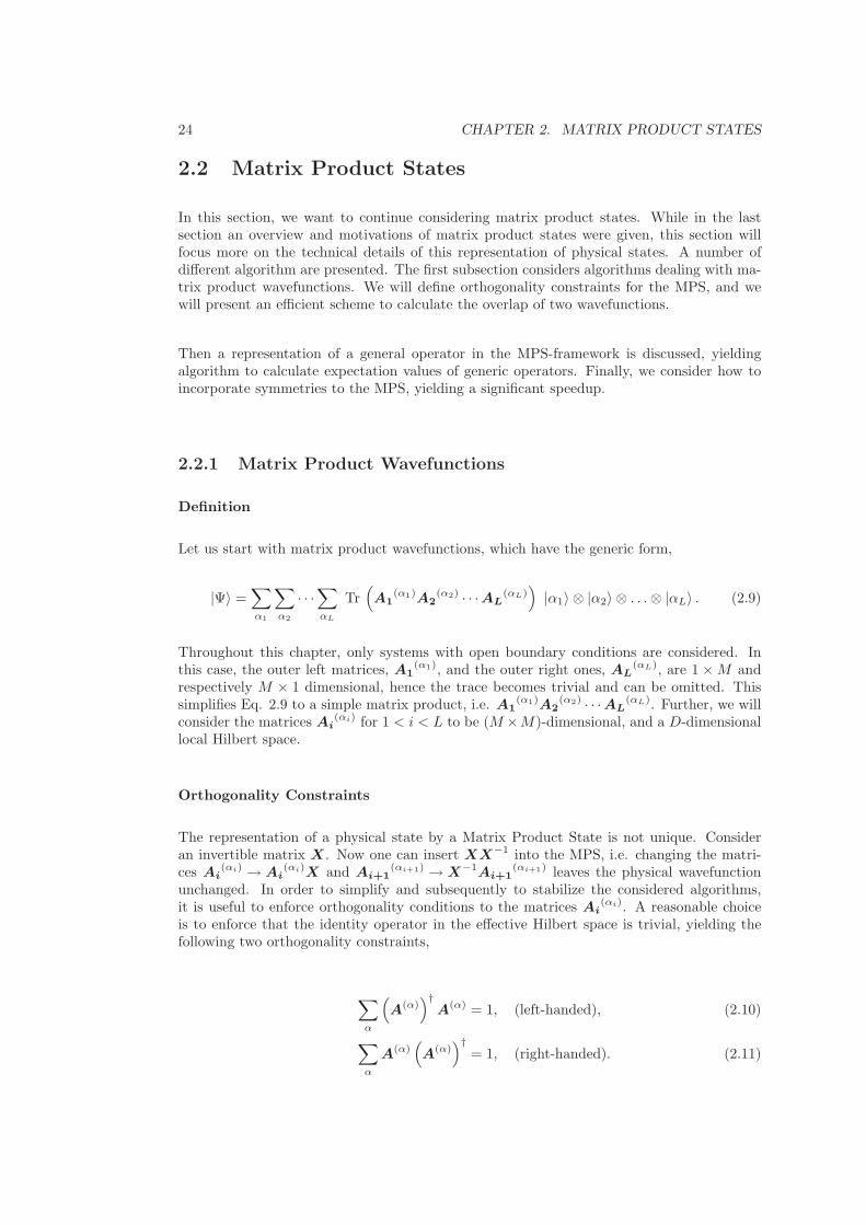
2.2 Matrix Product States
In this section, we want to continue considering matrix product states. While in the lastsection an overview and motivations of matrix product states were given, this section willfocus more on the technical details of this representation of physical states. A number ofdifferent algorithm are presented. The first subsection considers algorithms dealing with ma-trix product wavefunctions. We will define orthogonality constraints for the MPS, and wewill present an efficient scheme to calculate the overlap of two wavefunctions.
Then a representation of a general operator in the MPS-framework is discussed, yieldingalgorithm to calculate expectation values of generic operators. Finally, we consider how toincorporate symmetries to the MPS, yielding a significant speedup.
2.2.1 Matrix Product Wavefunctions
Definition
Let us start with matrix product wavefunctions, which have the generic form,
|Ψ〉 =∑
α1
∑
α2
· · ·∑
αL
Tr(
A1(α1)A2
(α2) · · ·AL(αL)
)
|α1〉 ⊗ |α2〉 ⊗ . . . ⊗ |αL〉 . (2.9)
Throughout this chapter, only systems with open boundary conditions are considered. Inthis case, the outer left matrices, A1
(α1), and the outer right ones, AL(αL), are 1 × M and
respectively M × 1 dimensional, hence the trace becomes trivial and can be omitted. Thissimplifies Eq. 2.9 to a simple matrix product, i.e. A1
(α1)A2(α2) · · ·AL
(αL). Further, we willconsider the matrices Ai
(αi) for 1 < i < L to be (M ×M)-dimensional, and a D-dimensionallocal Hilbert space.
Orthogonality Constraints
The representation of a physical state by a Matrix Product State is not unique. Consideran invertible matrix X. Now one can insert XX−1 into the MPS, i.e. changing the matri-ces Ai
(αi) → Ai(αi)X and Ai+1
(αi+1) → X−1Ai+1(αi+1) leaves the physical wavefunction
unchanged. In order to simplify and subsequently to stabilize the considered algorithms,it is useful to enforce orthogonality conditions to the matrices Ai
(αi). A reasonable choiceis to enforce that the identity operator in the effective Hilbert space is trivial, yielding thefollowing two orthogonality constraints,
∑
α
(
A(α))†
A(α) = 1, (left-handed), (2.10)
∑
α
A(α)(
A(α))†
= 1, (right-handed). (2.11)

2.2. MATRIX PRODUCT STATES 25
c)
d)
a)
b)
A1
∗
A2
∗
A2
∗
A3
∗
A3
∗A3
∗
A4
∗
A4
∗
A4
∗
A4
∗
B1
B2
B2
B3
B3B3
B4
B4
B4
B4
E1
E2
E3
Figure 2.5: Sketch of the scheme used to calculate overlaps. The lines depict the contractionof the indices. The overlap is given by Eq. 2.14, (a). Now, we can sum up the first physicalindex α1, yielding the M ×M matrix E1, shown in (b). The second site can be included, byusing Eq. 2.17, one obtains the new M × M matrix E2, (c). This scheme can be repeatediteratively, (d), E4 (not shown) finally contains the value of the overlap. The costs of thisscheme are cubic in the matrix dimensions and linear in the system size, i.e. O
(LM3
).
Consider a site i. When all matrices left of this site, i.e. all Aj for 1 ≤ j < i, fulfill theleft-handed constraint, the effective left basis set given by
∣∣∣l(i−1)
γ
⟩
=∑
α1
· · ·∑
αi−1
(
A1(α1) · · ·Ai−1
(αi−1))
γ|α1〉 ⊗ . . . ⊗ |αi−1〉 , (2.12)
is orthonormalized. Subsequently, when all matrices right of this site (i < j ≤ L) obey theright-handed condition, the effective right basis set, given by
∣∣∣r(i+1)
γ
⟩
=∑
αi+1
· · ·∑
αL
(
Ai+1(αi+1) · · ·AL
(αL))
γ|αi+1〉 ⊗ . . . ⊗ |αL〉 , (2.13)
is also orthonormalized.
Overlaps
Consider now two wavefunctions |ΨA〉 and |ΨB〉, given by the matrices Ai(αi) and Bi
(αi).The overlap 〈ΨA|ΨB〉 is now given by
〈ΨA|ΨB〉 =∑
{αi}
(
A1(α1)∗A2
(α2)∗ · · ·AL(αL)∗
)(
B1(α1)B2
(α2) · · ·BL(αL)
)
. (2.14)
This expression, however, involves a sum over a complete basis of the full Hilbert space, i.e.DL terms, making it unfeasible to evaluate numerically. Fig. 2.5 (a) sketches index contrac-tions needed to evaluate Eq. 2.14. By using the direct tensor product, (A ⊗ B)ii′jj′ = AijBi′j′ ,
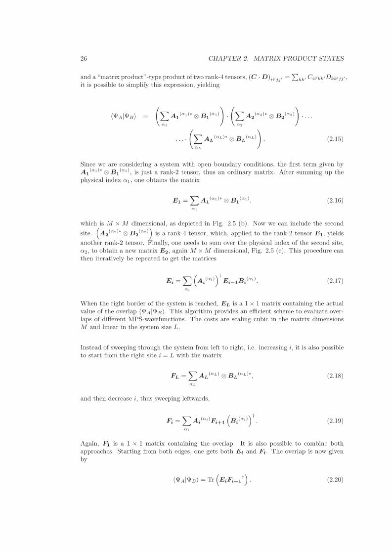
26 CHAPTER 2. MATRIX PRODUCT STATES
and a “matrix product”-type product of two rank-4 tensors, (C · D)ii′jj′ =∑
kk′ Cii′kk′Dkk′jj′ ,it is possible to simplify this expression, yielding
〈ΨA|ΨB〉 =
(∑
α1
A1(α1)∗ ⊗ B1
(α1)
)
·(
∑
α2
A2(α2)∗ ⊗ B2
(α2)
)
· . . .
. . . ·(
∑
αL
AL(αL)∗ ⊗ BL
(αL)
)
. (2.15)
Since we are considering a system with open boundary conditions, the first term given byA1
(α1)∗ ⊗ B1(α1), is just a rank-2 tensor, thus an ordinary matrix. After summing up the
physical index α1, one obtains the matrix
E1 =∑
α1
A1(α1)∗ ⊗ B1
(α1), (2.16)
which is M × M dimensional, as depicted in Fig. 2.5 (b). Now we can include the second
site.(
A2(α2)∗ ⊗ B2
(α2))
is a rank-4 tensor, which, applied to the rank-2 tensor E1, yields
another rank-2 tensor. Finally, one needs to sum over the physical index of the second site,α2, to obtain a new matrix E2, again M ×M dimensional, Fig. 2.5 (c). This procedure canthen iteratively be repeated to get the matrices
Ei =∑
αi
(
Ai(αi)
)†Ei−1Bi
(αi). (2.17)
When the right border of the system is reached, EL is a 1 × 1 matrix containing the actualvalue of the overlap 〈ΨA|ΨB〉. This algorithm provides an efficient scheme to evaluate over-laps of different MPS-wavefunctions. The costs are scaling cubic in the matrix dimensionsM and linear in the system size L.
Instead of sweeping through the system from left to right, i.e. increasing i, it is also possibleto start from the right site i = L with the matrix
FL =∑
αL
AL(αL) ⊗ BL
(αL)∗, (2.18)
and then decrease i, thus sweeping leftwards,
Fi =∑
αi
Ai(αi)Fi+1
(
Bi(αi)
)†. (2.19)
Again, F1 is a 1 × 1 matrix containing the overlap. It is also possible to combine bothapproaches. Starting from both edges, one gets both Ei and Fi. The overlap is now givenby
〈ΨA|ΨB〉 = Tr(
EiFi+1†)
. (2.20)

2.2. MATRIX PRODUCT STATES 27
|α1〉 |α2〉 |α3〉 |αL−2〉 |αL−1〉 |αL〉
|β1〉 |β2〉 |β3〉 |βL−2〉 |βL−1〉 |βL〉
C1 C2 C3 CL−2 CL−1 CL
Figure 2.6: Sketch of a matrix product operator.
In order to increase the stability of the algorithms, it is useful to enforce the orthogonalityconstraints just discussed, which are given by Eq. 2.10 and Eq. 2.11. The matrices Ai used tocalculate Ei should be left-orthonormalized, while the ones used for Fi right-orthonormalized.
MPS arithmetic
Finally, we want to consider the addition of two MPS wavefunctions, |ΨA〉 and |ΨB〉, given
by the matrices Ai(αi) and Bi
(αi). A new matrix product wavefunction for which |ΨC〉 =
|ΨA〉 + |ΨB〉 holds can be constructed by using the direct sum3 of the matrices Ai(αi) and
Bi(αi),
Ci(αi) = Ai
(αi) ⊕ Bi(αi). (2.21)
The matrix dimension of the new state is the sum of the dimensions of |ΨA〉 and |ΨB〉, i.e.MC = MA + MB , thus the space of matrix product states with a fixed maximal matrixdimension is not closed under the addition.
2.2.2 Matrix Product Operators
Introduction
In the last subsection, matrix product wavefunctions have been considered. However, it ispossible to extend the concepts of matrix product states to represent general operators. Ageneral matrix product operator is given by
C =∑
{αi},{βi}C1
(α1,β1)C2(α2,β2) · · ·CL
(αL,βL) |α1〉 〈β1| ⊗ |α2〉 〈β2| ⊗ . . .⊗ |αL〉 〈βL| , (2.22)
where Ci are rank-4 tensors, each physical index (αi and βi) is D-dimensional, and Ci(αi,βi)
are m × m dimensional matrices. Fig. 2.6 shows a sketch of a matrix product operator.
3The direct sum of two matrices A and B is given by A⊕ B =
»
A 00 B
–
.

28 CHAPTER 2. MATRIX PRODUCT STATES
Consider now an operator which can be written as a sum of local operator acting only on asingle site,
C =
L∑
i=1
Xi, (2.23)
where each local operator is given by Xi =∑
αiβi(Xi)αiβi
|αi〉 〈βi|. The operator C caneasily be written as a matrix product operator with the following matrices,
Ci(αi,βi) =
(δαi,βi
0(Xi)αi,βi
δαi,βi
)
, for 1 < i < L, (2.24)
C1(α1,β1) =
((X1)α1,β1
, δα1,β1
), and CL
(αL,βL) =(δαL,βL
, (XL)αL,βL
)T. Thus every oper-
ator which is a sum of local operators can always be represented as a 2 × 2 matrix productoperator. This scheme can be extended to operators containing next-nearest interactions ofthe form,
C =
L−1∑
i=1
XiYi+1, (2.25)
where both Xi and Yi are single site operators. The matrix product operator representationof C is now given by
Ci(αi,βi) =
δαi,βi0 0
(Yi)αi,βi0 0
0 (Xi)αi,βiδαi,βi
, for 1 < i < L, (2.26)
C1(α1,β1) =
(0, (X1)α1,β1
, δα1,β1
), and CL
(αL,βL) =(δαL,βL
, (YL)αL,βL, 0
)T. This can eas-
ily be generalized to arbitrary finite-range operators. Now, one can express the HamiltonianH of a system by a Matrix Product Operator. For commonly used one-dimensional Hamil-tonians the resulting matrix dimensions are small, for instance m = 3 for an Ising model ina transverse field or m = 6 for a fermionic Hubbard model, [38].
Operator Arithmetic
It is possible to calculate the sum of two matrix product operators (A and B, with the
matrices Ai(αi,βi) and Bi
(αi,βi)) directly by using the direct sum of the occurring matrices,similar to the sum of two wavefunctions considered in the last subsection,
Ci(αi,βi) = Ai
(αi,βi) ⊕ Bi(αi,βi). (2.27)
The matrix dimensions of the resulting operator (C = A+ B) are just the sum of the dimen-sions of each initial operator, i.e. mC = mA + mB .

2.2. MATRIX PRODUCT STATES 29
a) b)
A1
∗ A2
∗ A3
∗A3
∗ A4
∗ A5
∗
B1 B2 B3B3 B4 B5
C1 C2
C3
C3 C4 C5E2 F4
∗
Figure 2.7: Scheme to calculate expectation values: (a) expression to evaluate and (b) ex-pression after applying both Eq. 2.30 and Eq. 2.31 twice.
The product of the two operators C = AB) can also be calculated, the matrices of theresulting matrix product operator are given by a sum of direct products,
Ci(αi,βi) =
∑
γi
Ai(αi,γi) ⊗ Bi
(γi,βi), (2.28)
with the matrix dimensions mC = mAmB .
Applying an Operator
It is possible to apply a matrix product operator exactly on a matrix product wavefunction.Given the wavefunction |ΨA〉 with the matrices Ai
(αi) and the operator C, represented byEq. 2.22, one can write down a new wavefunction |ΨB〉 ≡ C |ΨA〉 with the mM × mMdimensional matrices
Bi(αi) =
∑
γi
Ci(αi,γi) ⊗ Ai
(γi). (2.29)
Expectation Values
One can use this algorithm to calculate expectation values of arbitrary operators by firstapplying the operator to one wavefunction and then calculating the overlap as described inthe last section. However, one can construct a more efficient scheme for evaluating expressionsof the type 〈ΨA| C |ΨB〉. The scheme is similar to the one used to calculate overlaps asdiscussed in the last subsection. Starting from the left one obtains the following matrices,
Ei(ηi) =
∑
αiβiηi−1
(
Ci(αi,βi)
)
ηiηi−1
(
Ai(αi)
)†Ei−1
(ηi−1)Bi(βi). (2.30)
If starting from the right, one gets
Fi(ηi−1) =
∑
αiβiηi
(
Ci(αi,βi)
)
ηiηi−1
Ai(αi)Fi+1
(ηi)(
Bi(βi)
)†. (2.31)

30 CHAPTER 2. MATRIX PRODUCT STATES
Note the additional index ηi which is introduced by matrix products of the matrix productoperator. The final value of the expectation value is then given by
〈ΨA| C |ΨB〉 =∑
ηi
Tr
(
Ei(ηi)
(
Fi+1(ηi)
)†)
. (2.32)
The overlap scheme is sketched in Fig. 2.7.
Conclusion
In this section, matrix product operators were introduced. Compared with the naıve formu-lation of the DMRG algorithm, the MPS approach offers great flexibility. Any expectationvalue or correlator can directly be calculated, one does not need to keep track of the repre-sentations of the operators in the effective basis set as in the naıve formulation, it sufficesto know the current wavefunction and MPO representation of the operator. Further, it ispossible to calculate operators like H2, since the matrix dimensions m of the Hamiltonianare usually small and thus H2 with the dimensions m2 is easy to handle. This can be used
to evaluate the variance of a state, i.e. σ2 =⟨
H2⟩
−⟨
H⟩2
, which gives a bound of error of
a calculated wavefunction (this will be discussed in more detail in the next section).
2.2.3 Symmetries
Now, we want to also include symmetries of the Hamiltonian in the MPS framework. Considera Heisenberg model
H =
N−1∑
i=1
[JxSx
i Sxi+1 + JySy
i Syi+1 + JzS
zi Sz
i+1
], (2.33)
where ~Si ≡ (Sxi , Sy
i , Szi )
Tare the usual spin-S operators.
If all interaction strengths are unequal, i.e. Jx 6= Jy 6= Jz the system does not possess anyglobal symmetry. However, if two interactions are equal, i.e. Jx = Jy 6= Jz, a rotation sym-
metry along the z-axis emerges, given by the unitary symmetry operator T (α) = exp(
iαSz
)
,
where Sz ≡ ∑
i Szi is the total spin in z-direction, and the symmetry group U(1). This yields
a conserved quantity⟨
Sz
⟩
, as Sz commutes with the Hamiltonian.
Now, we want to consider general Abelian symmetries, for example the Sz, U(1) spin symme-try or the U(1) particle number conservation symmetry, for instance present in the Hubbardmodel (both fermionic and bosonic). Any Abelian group has a one-dimensional irreduciblerepresentation, yielding a conserved quantum number q.
This allows us to represent the A-matrices as irreducible tensors, for which Akqlqr
is onlynon-vanishing if qr = ql + k holds. Here ql and qr are the quantum numbers associatedwith the left and the right effective basis states, and k is the quantum number of the local

2.2. MATRIX PRODUCT STATES 31
states. This scheme differs from the scheme used in the usual DMRG algorithm, where oneconstructs the superblock wavefunction (see section 2.3 for more details)
|Ψ〉 =∑
uv
Cuv |u〉 ⊗ |v〉 , such that (u + v = target) holds. (2.34)
However, the scheme used here is different. The left vacuum state has the quantum number0, and the right vacuum state the target quantum number. Therefore, it is only possible totarget one quantum number using one MPS state, while the DMRG allows to simultaneouslytarget multiple quantum numbers. Nevertheless, due to the great flexibility of the MPS ap-proach, which allows to deal with more than one MPS state simultaneously, this does notimpose any restrictions.
Let us now consider the case where all three interaction strengths of the Heisenberg modelare equal, Jx = Jy = Jz. Then one obtains a full rotation symmetry which is parametrized
by T (α, β, γ) = exp(
iαSx
)
exp(
iβSz
)
exp(
iγSx
)
, and the symmetry group SU(2). This
group is no longer Abelian, however, using the Wigner - Eckert theorem, [40],
〈j,m|T [k]M |j′,m′〉 = 〈j‖T [k] ‖j′〉Cj k j′
mMm′ , (2.35)
it is again possible to construct the A-matrices as irreducible tensors, for more details see[41], and [42, 43].
Making use of the symmetries yields significantly faster algorithms. The matrices becomeblock-diagonal, and as the computational costs of the MPS algorithm scale roughly cubic inthe matrix sizes, one gains a considerably speedup. Including non-abelian symmetries usuallyreduces the computational costs by another order of magnitude, see section 2.3.3 and [41].

32 CHAPTER 2. MATRIX PRODUCT STATES
Figure 2.8: Sweeping scheme used in DMRG. One performs local optimizations, starting fromthe left end of the system and moving to the right. When the end is reached, the directionis changed and one moves back to the left end.
2.3 DMRG
In this section, we want to formulate the density matrix renormalization group (DMRG)algorithm [11, 12] with matrix product states. The general goal of this section is to calculategroundstates, but the presented concepts can also be used to create a variety of other algo-rithms, like the solution of time-dependent problems, which will be discussed in section 2.4,and the calculation of dynamical spectral functions, discussed in section 2.5.
2.3.1 Local Optimization
A key ingredient of all considered algorithms are local optimizations. Instead of performingglobal updates (which would in general be an intractable problem), one only locally opti-mizes the wavefunction by changing only one (or a few) A-matrices at once. This naturallyintroduces a sweeping procedure, i.e. the optimization of the state starts for example fromthe left edge of the system and goes towards the right end. When one reaches the right end,the direction is switched and one goes back to the left end, and so forth. Fig. 2.8 sketchesthe described sweeping scheme. This procedure is repeated until the state is sufficiently con-verged.
A convenient approach to perform local optimization is based on the so-called center matrix.Consider a matrix product state where between the matrices Ai
(αi) and Ai+1(αi+1) a center
matrix C is inserted,
|Ψ〉 =∑
{αi}A1
(α1)A2(α2) · · ·Ai
(αi)CAi+1(αi+1) · · ·AL
(αL)∣∣∣{αi}
⟩
. (2.36)
It is always possible to insert or remove a center matrix to a matrix product state withoutchanging the physical state, Now, one can enforce the orthogonalization constraints con-sidered in section 2.2.1 for all A-matrices. All matrices left of the bond, where the centermatrix is located, i.e. Aj for 1 ≤ j ≤ i, are left-orthogonalized, all others right of the bond(i + 1 ≤ j ≤ L) are right-orthogonalized. Thus, both effective basis sets (given by Eq. 2.12and Eq. 2.13) are orthonormalized, and the wavefunction is given by

2.3. DMRG 33
|Ψ〉 =∑
γγ′
Cγγ′
∣∣∣l(i)γ
⟩
⊗∣∣∣r
(i+1)γ′
⟩
. (2.37)
This form of the wavefunction corresponds to the so-called superblock wavefunction in DMRGlanguage. By using the E(η) and F (η) matrices, given by considering 〈Ψ| H |Ψ〉, one gets a
representation of the Hamiltonian in the effective basis∣∣∣l
(i)γ
⟩
⊗∣∣∣r
(i+1)γ′
⟩
.
Now, we need to calculate the groundstate of this effective Hilbert space. It turns outthat Krylov subspace-based algorithms are well suited to solve this problem. The old centermatrix can be used as an initial guess vector, as it is a reasonable approximation to the correctsolution. This enhances the speed of convergence of the Krylov subspace-based method. TheHamiltonian H is Hermitian, hence a Lanczos iteration scheme, similar to the one used insection 2.4.2, can be applied to get an orthonormalized Krylov basis. For more details onthe Lanczos iteration and Krylov subspace methods in general see [44].
2.3.2 Truncation
In the algorithm presented in the last subsection, a M×M center matrix is locally optimized.However, a significant improvement can be gained if the effective Hilbert space is enlarged.
Instead of considering only the effective Hilbert space spanned by∣∣∣l
(i)γ
⟩
⊗∣∣∣r
(i+1)γ′
⟩
, one can
enlarge the effective Hilbert space by fully taking the local physical Hilbert space into account,
i.e. by considering the space spanned by∣∣∣l
(i−1)γ
⟩
⊗ |αi〉 ⊗∣∣∣r
(i+1)γ′
⟩
, when the left site is
expanded, or spanned by∣∣∣l
(i)γ
⟩
⊗ |αi+1〉 ⊗∣∣∣r
(i+2)γ′
⟩
for the right site. Both expansions can be
incorporated into the center matrix approach. Let us only consider an expansion of the left
site. Transform Ai(αi) into a M ×DM dimensional identity matrix A′
i
(αi), in the sense that
A′
i
(αi)
γi−1γ′ = δγ′,(γi−1+Dαi) (2.38)
and add a DM × M dimensional center matrix matrix given by
C(γi−1+Dαi),γi= Ai
(αi)γi−1γi
, (2.39)
introducing the new index γ′ ≡ γi−1 +Dαi. This transformation leaves the state unchanged.
By using the algorithm described in the last subsection, 2.3.1, one can now locally optimizethe DM ×M -dimensional center matrix (in the case when the left site is expanded, otherwiseit is M ×DM -dimensional). These schemes are commonly referred as one site algorithm [45].It is also possible to expand both sites, yielding a DM × DM dimensional center matrix,which is the scheme used in traditional DMRG and referred as two site algorithm.
However, these schemes increase the matrix dimensions of the MPS. As the computationalcosts scale roughly cubic with the matrix dimensions, a truncation of the matrix dimensions

34 CHAPTER 2. MATRIX PRODUCT STATES
at some point of the algorithm is required.
Let us first consider the two-site algorithm. The center matrix is (DM ×DM)-dimensional.Now it is possible to write down the density matrix of the left (and right) subsystem
ρL =∑
γγ′η
CγηC∗γ′η
∣∣∣l(i)γ
⟩ ⟨
l(i)γ′
∣∣∣ , and (2.40)
ρR =∑
γγ′η
CηγC∗ηγ′
∣∣∣r(i+1)
γ
⟩ ⟨
r(i+1)γ′
∣∣∣ . (2.41)
By using the Schmidt-decomposition (given by Eq. 2.2) of the density matrix, which diago-nalizes the density matrix,
ρ =
DM∑
i=1
pi |i〉 〈i| , (2.42)
and keeping only M terms with the highest coefficients pi, one can set up a truncation scheme.This truncation scheme keeps only the terms with the highest entropy.
This scheme is closely related to the singular value decomposition of the center matrix,given by C = U †DV , where U and V are DM × DM dimensional unitary matrices, andD a DM × DM dimensional diagonal matrix with the non-negative diagonal entries
√pi,√
p1 ≥ √p2 ≥ . . . ≥ √
pr > 0. Again, one can truncate this decomposition such that only Mterms with the highest weights are kept.
The sum of the discarded weights is usually referred as truncation error,
r =
DM∑
i=M+1
pi. (2.43)
What happens when considering the one-site algorithm? The center matrix becomes M ×DM dimensional, thus the matrix rank of the center matrix cannot be bigger than M .Therefore, the truncation scheme just discussed does not alter the wavefunction at all, hencethe truncation error always vanishes. This increases the chance that the algorithm getstrapped in a metastable state. It is possible to circumvent this problem by adding a smallperturbation term to the density matrix,
ρL =∑
γγ′
(
CC† + f∑
αi
Ei(αi)CC†
(
Ei(αi)
)†)
γγ′
∣∣∣l(i)γ
⟩ ⟨
l(i)γ′
∣∣∣ , and (2.44)
ρR =∑
γγ′
(
C†C + f∑
αi
Fi+1(αi)C†C
(
Fi+1(αi)
)†)
γγ′
∣∣∣r(i+1)
γ
⟩ ⟨
r(i+1)γ′
∣∣∣ . (2.45)

2.3. DMRG 35
10-4
10-3
10-2
10-1
100
0 25 50 75
(wav
efun
ctio
n di
ffere
nce)
2
sweep number
Figure 2.9: The convergence of the DMRG sweeping scheme: the change of the wavefunctionafter one sweep squared is plotted against the number of performed sweeps. After approxi-mately 50 sweeps, the DMRG algorithm converges.
f is the mixing factor. This disturbed density matrix prevents the trapping in the metastablestates.
Since the one-site algorithm only operates with M ×DM dimensional matrices instead of theDM ×DM dimensional matrices of the two-site approach, it is usually the faster algorithm.Further, the speed of convergence is also better. However, the two-site algorithm has a betterstability when considering frustrated systems[46].
2.3.3 Application of the Algorithms
In this subsection we want to present some illustrative results for an isotropic spin-1/2 Heisen-berg model, given by Eq. 2.33, with a system size of L = 256.
Starting from a random matrix product state with small matrix dimensions (usually M < 10),it is useful to perform a reasonable number of DMRG sweeps with a small number of stateskept (of the order of 20 – 50) until the wavefunction is converged. A good convergence testis given by considering the norm of change of the wavefunction before and after a DMRG
sweep, i.e.∥∥∥ |Ψi+1〉−|Ψi〉
∥∥∥
2
. While this quantity is not available in the old DMRG language,
it can easily be calculated in the MPS framework. Fig. 2.9 shows this quantity as functionof the number of performed sweeps. After approximately 50 sweeps a convergence can beobserved in this example.
When the DMRG is converged with a small number of states, one can increase M to thefinal number of states. Starting directly with the final number of states is not efficient, as

36 CHAPTER 2. MATRIX PRODUCT STATES
10-8
10-7
10-6
10-5
10-4
10-3
10-8 10-7 10-6 10-5 10-4 10-3
E-E
0
(H - E)2
DMRGfit
Figure 2.10: Energy error(⟨
H⟩
− E0
)
as function of the variance σ2 ≡⟨
(H − E)2⟩
for
a S = 1/2 Heisenberg model, L = 256, one site algorithm, mixing factor f = 0.01,and different number of states are kept, M = 50 − 350. The fitted function is given by(0.86 ± 0.04) x1.04±0.01 + O
(10−12
).
the number of sweeps needed to transform the initial random state to the converged stateis roughly independent of the number of states kept. However, as the computational costsscale cubic with the number of states kept, a significant efficiency gain can be obtained if onestarts with a small number of states.
After the state is converged, one can calculate the desired physical observables, for instancecorrelation functions. Using matrix product states the calculation of the groundstate is avariational procedure[46]. The quality of this approximation is related to the variance of
the obtained state, given by⟨
H2⟩
−⟨
H⟩2
. The variance of an eigenstate is zero and for
non-eigenstate it measures the distance of the state from the next eigenstate. Now we canperform an extrapolation in the variance of the obtained physical quantities. In Fig. 2.10 anextrapolation of the groundstate energy is shown. The difference of the obtained groundstateenergy and the exact groundstate energy4 as a function of the variance is plotted. The errorscales roughly linear in the variance, as indicated by the fit.
To conclude the discussion of the DMRG algorithm, we want to discus the effects of using thenon-abelian symmetries, as discussed in section 2.2.3. Table 2.1 shows the variance as functionof the number of states. Each non-abelian symmetry reduces the variance significantly,illustrating that keeping M SU(2) invariant states is rather different from keeping M Abelianstates. The algorithm which handles the non-abelian symmetries requires slightly highercomputational effort for a fixed number of states, but, however, an overall speedup of morethan one order of magnitude is gained by each considered non-abelian symmetry.
4obtained by further increasing M and making use of the non-abelian SU(2) symmetry such that the erroris of the order of the machine precision, i.e. ∼ 10−16.

2.3. DMRG 37
(a)
M U(1) SU(2)
20 1.29 · 10−2 2.18 · 10−4
50 7.29 · 10−4 1.88 · 10−6
100 4.33 · 10−5 1.52 · 10−8
200 9.61 · 10−7 ∼ 10−10
(b)
M U(1) × U(1) U(1) × SU(2) SU(2) × SU(2)
50 2.29 · 10−2 1.54 · 10−3 4.33 · 10−6
100 3.32 · 10−3 7.60 · 10−5 3.85 · 10−8
200 2.50 · 10−4 2.02 · 10−7 1.92 · 10−10
400 1.23 · 10−5 2.93 · 10−8 ∼ 10−12
Table 2.1: Variance⟨
(H − E)2⟩
for different number of kept states M , and making use
of different symmetries. In (a) a spin-1/2 Heisenberg model with the length L = 256 isconsidered, and in (b) a half-filled Hubbard model with the system parameter L = 32,U = 4, and t = 1 is considered.

38 CHAPTER 2. MATRIX PRODUCT STATES
2.4 Time-Dependent Problems
In this section we want to present algorithms which calculate the time-evolution of a state|Ψ(t = 0)〉 for a given Hamiltonian H by using Matrix Product states. In general the time-evolution of a Hamiltonian, which does not depend on the time itself, can be written by usingthe operator exponential, i.e.
|Ψ(t)〉 = exp(
iHt)
|Ψ(t = 0)〉 . (2.46)
In a number of physical situations the calculation of the time-evolution is desirable. Con-sider an ultracold atomic gas in an optical lattice. Due to the good control over the systemparameter and especially the good tunability, it is possible to observe out-of-equilibrium ef-fects. In [98], a sudden increase of the onsite interaction (induced by increasing the latticedepth) quenched the system. While the system is initially in a superfluid phase, the phaseis destroyed by the quench. A Mott insulator-like state appears, followed by a revival of thesuperfluid phase. In order to fully understand this and similar effects, an exact treatment ofthe time-evolution is necessary.
Dynamic response functions, i.e. G(t) = 〈gs| A(0) A(t) |gs〉, are a key tool for the understand-ing of condensed matter systems. While algorithms for calculating the Fourier transform ofthe Green function, i.e. G(ω) =
∫dt exp (iωt) G(t), will be discussed in the next section,
2.5, one can use the algorithm presented in this section to obtain the real-time Green function.
Let us now come back to the MPS algorithm. It is useful to discretize the time and to calculateeach timestep separately. Hence for a timestep ∆t, we want to consider the wavefunction|Ψj〉 ≡ |Ψ(tj)〉 at the times tj = j ∆t. Thus, for each timestep one exponential needs to beapplied to the wavefunction,
|Ψj+1〉 = exp(
iH∆t)
|Ψj〉 . (2.47)
In the following subsections we first want to introduce two different algorithms for calculat-ing the time-evolution. One algorithm is based on a Trotter decomposition of the matrixexponential. The second algorithm is based on a Krylov subspace expansion of the matrixexponential. Finally both algorithms will be compared in the last subsection 2.4.3.
2.4.1 Trotter Decomposition
The first algorithm we want to discuss is based on the Trotter decomposition of the operatorexponential. Let us start with considering the usual Trotter decomposition of a matrixexponential. Let A and B be two square matrices. The first order Trotter decomposition of
exp(
δ(A + B))
is given by
exp(
δ(A + B))
= exp(
δA)
exp(
δB)
+ O(δ2
). (2.48)
Higher orders of the Trotter decomposition can easily be constructed,

2.4. TIME-DEPENDENT PROBLEMS 39
exp(
δ(A + B))
= exp(δ
2A
)
exp(
δB)
exp(δ
2A
)
︸ ︷︷ ︸
≡S2th(δ)
+O(δ3
), (2.49)
is a second order decomposition, a fourth order one is given by (ϑ−1 ≡ 2 − 3√
2),
exp(
δ(A + B))
= S2th
(
ϑδ)
· S2th
(
(1 − 2ϑ)δ)
· S2th
(
ϑδ)
+ O(δ5
). (2.50)
It is also possible to construct decomposition with higher orders, for more details see [47].
Consider now a system where the Hamiltonian can be decomposed in two parts, one whichonly acts on even bonds, the other only on odd bonds. This is always possible for a one-dimensional system where interaction only couples next-nearest neighbors. The Hamiltonianis now given by the sum of both parts, i.e.
H = Heven + Hodd. (2.51)
A local part of the interaction can also be included, it is convenient to split this part suchthat it contributes in either parts to both the even and the odd Hamiltonian. Consider aBose-Hubbard model (which will be discussed in section 4.2.1) to illustrate this procedure.The Hamiltonian is given by
H = −J
L−1∑
i=1
(
b†i bi+1 + b†i+1bi
)
+U
2
L∑
i=1
ni (ni − 1) . (2.52)
Now, one can split the Hamiltonian into (L− 1) terms acting only on a single bond (L shallbe even). Each part can now be written down,
Hi = −J(
b†i bi+1 + b†i+1bi
)
+U
4
(
ni (ni − 1) + ni+1 (ni+1 − 1))
+ Hborderi , (2.53)
where Hborderi is an additional term5 reflecting the open boundary conditions, being only
non-zero for i = 1 and i = (L− 1). The even and the odd part of the Hamiltonian are givenby,
Heven =
L/2−1∑
i=1
H2i, Hodd =
L/2∑
i=1
H2i−1. (2.54)
Now we can apply the Trotter decomposition to the operator exponential of the time-evolution, given by Eq. 2.47. For the sake of simplicity, let us consider only a first orderTrotter decomposition here, for higher orders the described scheme can be performed inexactly the same manner. The first order decomposition is given by,
5The exact form of this term is given by, Hborderi
=
8
<
:
U/4 n1(n1 − 1), i = 1U/4 nL(nL − 1), i = (L − 1)0, else

40 CHAPTER 2. MATRIX PRODUCT STATES
exp(
iH∆t)
= exp(
iHeven∆t)
exp(
iHodd∆t)
+ O(∆t2
). (2.55)
Each even bond Hamiltonian commutes with every other even bond Hamiltonian, and every
odd with every other odd bond Hamiltonian,[
H2i, H2j
]
= 0, and[
H2i−1, H2j−1
]
= 0.
Thus, we can decompose the exponential into products of operator exponentials which onlyact on single bonds,
exp
i
L/2−1∑
i=1
H2i∆t
=
L/2−1∏
j=1
exp(
iH2j∆t)
, (2.56)
exp
i
L/2∑
i=1
H2i−1∆t
=
L/2∏
j=1
exp(
iH2j−1∆t)
. (2.57)
It is possible to evaluate the action of such operators on a Matrix Product State exactly.Starting from the left border of the system one can apply the odd bond evolution operators,while sweeping towards the right end. Then the even evolution operators can be applied inthe other direction. One timestep is finally given by,
|Ψj+1〉 ≈ exp(
iH2∆t)
× exp(
iH4∆t)
× · · · × exp(
iHL−2∆t)
×
exp(
iHL−1∆t)
× exp(
iHL−3∆t)
× · · · × exp(
iH1∆t)
|Ψj〉 . (2.58)
While sweeping through the system it is useful to truncate the MPS, either by limiting thenumber of states used or by using a fixed truncation error.
Two sources of errors are present in the presented algorithm. First, the Trotter decompositionintroduces an error, for the first order Trotter decomposition this error is proportional to ∆t2.By considering higher order Trotter decomposition, like the second (Eq 2.49) and the fourthorder decomposition (Eq. 2.50), this error can be reduced. A further source of error stemsfrom the truncation of the MPS states. These errors will be discussed in more detail in thesection 2.4.3.
2.4.2 Krylov Subspace Methods
Now, we want to consider another algorithm which can be used to calculate the time-evolutionbased on a Krylov subspace expansion of the evolution operator. Let us start with a def-inition of the Krylov subspace. Consider a wavefunction |Ψ〉 and an operator H (i.e. theHamiltonian). The N-dimensional Krylov space is then spanned by the wavefunctions Hi |Ψ〉,i = 0, . . . , (N − 1), i.e. given by
KN
(
|Ψ〉 , H)
= span(
|Ψ〉 , H |Ψ〉 , H2 |Ψ〉 , . . . , HN−1 |Ψ〉)
. (2.59)
Since the Hamiltonian is a Hermitian operator, the Lanczos algorithm can be used to generatean orthonormal basis set of KN . Define the zeroth Krylov vector as |k0〉 ≡ |Ψj〉. The higher

2.4. TIME-DEPENDENT PROBLEMS 41
Krylov vectors are calculated by iteratively applying H. In order to obtain an orthonormalbasis set, one can use the following scheme (Lanczos iteration),
βi+1 |ki+1〉 = H |ki〉 − αi |ki〉 − βi |ki−1〉 , (2.60)
where αi and βi are chosen such that the orthonormality condition 〈ki|kj〉 = δij is fulfilled.
Now, the Hamiltonian of the system can be approximated using the Krylov vectors,
H ≈N−1∑
i,j=0
Hij |ki〉 〈kj | , Hij = 〈ki| H |kj〉 . (2.61)
With this approximation, it is now possible to exactly calculate the time-evolution given byEq. 2.47,
|Ψj+1〉 = exp(
iH∆t)
|Ψj〉 ≈N−1∑
n=0
cn |kn〉 , (2.62)
where the cn are given by the matrix exponential (H denotes the Hamiltonian in the Krylovspace, i.e. a N × N matrix),
cn =(
exp(iH∆t
))
n,0. (2.63)
The generated time-evolution operator is always unitary, thus the normalization of the wave-function is preserved.
The Krylov method can easily be adapted to matrix product states. Applying a (matrixproduct) operator to a MPS is straight-forward and can easily be performed exactly, as dis-cussed in the last section. A big advantage of the MPS formulation of the Krylov algorithm,is that it is possible to use a new MPS for each Krylov vector, hence one can exploit the fulllocal Hilbert space to represent each vector. However, when using old DMRG formulationwhere the local Hilbert space needs to be split among all Krylov vector, the number of neededstates is significantly increased. As the numerical cost of the used algorithms scales cubicwith the number of states, one obtains a large speedup of the algorithm when using separatematrix product states for each Krylov vector.
The matrix product operators introduced in the last section can be used to calculate theKrylov vectors exactly. However, the matrix dimensions for each Krylov vector |ki〉 will be-come rather large, especially for higher Krylov vectors (i.e. large i), thus a truncation of thestates is required, limiting the accuracy of the calculated Krylov vectors.
A further error is induced by limiting the Hamiltonian to the Krylov subspace. It can beshown that for sufficiently small timesteps the coefficients of the higher Krylov vectors areexponentially suppressed. This gives an estimate of the error made by considering only afinite number of Krylov vectors, which is roughly proportional to the coefficient of the last

42 CHAPTER 2. MATRIX PRODUCT STATES
Krylov vector |kN−1〉, i.e. cN−1 of Eq. 2.62.
Hochbruck and Lubrich [52] performed an error analysis for Krylov subspaces based algo-rithms for calculating matrix exponentials. Their main result is a strict error bound for the
calculated result, here |Ψj+1〉. Given the numerical obtained⟨
ki
∣∣∣kj
⟩
(which should be δij
without numerical errors) and further⟨
ki
∣∣∣ H
∣∣∣kj
⟩
and⟨
ki
∣∣∣ H2
∣∣∣kj
⟩
, they give a bound on
the error of∣∣∣ki
⟩
(induced by the truncation of the MPS). Together with the error induced
by the finite dimension of the Krylov subspace, one gets a bound ε for the total error of theresulting wavefunction given by
∥∥∥|Ψj+1〉 − exp
(
iH∆t)
|Ψj〉∥∥∥
2
< ε2. (2.64)
Thus, it is possible to set a fixed error bound ε for each timestep. Subsequently, the numberof Krylov vectors are iteratively increased, while the truncation error of each Krylov vector|ki〉 is adapted (starting from a big truncation error, which is iteratively decreased) such thatfinally the error bound given by Eq. 2.64 is fulfilled.
The presented algorithm allows a precise control over both the numerical errors and requiredprecision of each Krylov vector. This enables us to perform an efficient simulation of thetime-dependent problems (in terms of the computational costs) while having a strict boundon the numerical errors.
In the next subsection both algorithms, i.e. the Trotter decomposition and the Krylovalgorithm, are applied to a physical test case in order to assess both the accuracy and thecomputational costs of the algorithms.
2.4.3 Comparison
In this subsection, both algorithms are applied to a physical model, a spin-1/2 XXZ modeldescribed by the following Hamiltonian
H =
N−1∑
i=1
[1
2
(S+
i S−i+1 + S−
i S+i+1
)+ ∆Sz
i Szi+1
]
. (2.65)
~Si are spin-1/2 operators, and ∆ controls the anisotropy of the system. For ∆ > 1 thesystem favors a gapped anti-ferromagnetic phase, while for −1 < ∆ < 1 a critical phase canbe observed. At both ∆ = −1 and ∆ = 1, the system is at a quantum critical point. Formore details see [56].
Here we want to consider the time-evolution after a single particle (magnon) excitation astest case in order to assess the algorithms discussed in the subsections before. We choose∆ = 0.2 and a system size of L = 64. Similar to the single particle excitations which willbe considered in section 4.3.2, the spin ladder operator S+
L/2 is applied to the groundstate,

2.4. TIME-DEPENDENT PROBLEMS 43
10-8
10-6
10-4
10-2
100
0 2 4 6 8 10
erro
r2
t
Krylov, ε2 = 10-4, ∆t = 0.25Krylov, ε2 = 10-7, ∆t = 0.25ST2, ∆t = 0.125ST4, ∆t = 0.125ST2, ∆t = 0.05ST4, ∆t = 0.05
Figure 2.11: The absolute error squared of the time-evolution obtained by the Krylov time-evolution and different Trotter algorithms, as function of the time.
i.e. |Ψ(t = 0)〉 = S+1 |gs〉. The groundstate is first calculated by using DMRG, and the time-
evolution of the excited state is calculated.
In order to compare the different algorithms, we first calculated a quasiexact time-evolutionby the Krylov algorithm using a timestep of ∆t = 0.25 and an error bound per timestep ofε2 = 10−12. Based upon the analysis given in this subsection and with considering a forward-backward time-evolution, one can conclude that a reasonable error bound of the calculated
wavefunctions∣∣∣Ψ(t)
⟩
is given by
∥∥∥∥∥
∣∣∣Ψ(t)
⟩
−∣∣∣Ψ(t)
⟩∥∥∥∥∥
2
< 10−10. (2.66)
This quasiexact result can now be used as a reference result to assess the quality of thetime-evolution using a limited precision. Fig. 2.11 shows the squared wavefunction error asa function of time. Let us start with considering the Trotter algorithm, discussed in section2.4.1.
As discussed before, there are two different sources of errors present in the Trotter time-evolution. On the one hand, the Trotter decomposition is only an approximation to thematrix exponential. This error can be diminished by reducing the timestep and by con-sidering higher orders of the Trotter decomposition. On the other hand, the unavoidabletruncations of the MPS are the other source of errors. While keeping more states, i.e. in-creasing M , reduces the truncation error, one can also increase the timestep and thus reducethe overall number of truncations needed. Both sources of errors limit the possible timestepof the algorithm. If the timestep is too big, the Trotter errors are dominating, while if thetimestep is too small, the truncation errors are the main source of errors..

44 CHAPTER 2. MATRIX PRODUCT STATES
The Trotter decomposition, which was first considered in section 2.4.1, is the first order de-composition given by Eq. 2.48. However, the Trotter error is dominant and much biggerthan errors of the higher order decompositions, hence the first order decomposition is notuseful in this context. The second order decomposition reduces the Trotter error by a sig-nificant amount. Let us now consider the second order results shown in Fig. 2.11. Notethat all time-evolutions based on Trotter decompositions have been calculated with the sametruncation error of r = 10−10. Reducing the timestep of the second order Trotter algorithmreduces the errors by a considerable amount. Thus in this case the errors stem mainly fromthe Trotter error. This changes when considering the fourth order decomposition, given byEq. 2.50. The errors do not change much if the timestep is altered. Hence in this case, theerror is mainly introduced by the truncations.
Now we want to consider the Krylov-subspace based algorithms. A typical timestep used isof the order of 0.25 in the considered case, much bigger than the timesteps of the Trotteralgorithm. The timestep controls the number of Krylov vectors needed to faithfully representthe time-evolution exponential, Eq. 2.47. A reasonable number of Krylov vectors are 5- 8 vectors. If the timestep is further increased, and thus the number or Krylov vectors,it becomes more and more complicated to calculate the higher Krylov vectors involvinghigh powers of the Hamiltonian. This severely deteriorates the algorithm, good results areonly achievable by excessive consumption of computer resources. A threshold where theseproblems start to arise can be estimated by the inverse square root of variance of the state,
i.e. ∆t <
(⟨
H2⟩
−⟨
H⟩2
)− 12
. On the other hand, if the timestep is too small, the change
of the wavefunction by the time-evolution is too small, and will be truncated, thus againlimiting the precision of the algorithm.
Let us now consider the numerical results obtained by the Krylov algorithm. Fig. 2.11 showsthe errors of the Krylov time-evolution for different error bounds per timestep. First, notethat the error bound given by 2.64 is fulfilled for each timestep.
For the Krylov algorithm, there are two sources of errors present. Due to the finite precisionof the MPS states introduced by the truncation, the calculated Krylov vectors are containingnumerical errors. This yields non-unitary errors, which can be assessed by considering aforward-backward time-evolution. The state is first evolved up to a time t, and then oneperforms a backward time-evolution to get back to the initial state at t = 0. The differenceof the initial state and the state obtained by the forward-backward evolution measures nowthe non-unitary errors of the Krylov algorithm. On the other hand, since we are consideringonly a finite number of Krylov vectors, another error source is introduced.
In Fig. 2.12 we compare the exact error of the Krylov algorithm with the error obtainedby the forward-backward evolution. For small times up the order of t ∼ 3, one observes alinear dependence of the error with respect to the time6. For these times, the error is mainlygiven by the non-unitary errors, as both the exact error and the forward-backward errorare approximately the same. This changes for bigger times where the exact error increasesquadratically with respect to the time. However, one can note a big difference between theforward-backward error and the exact error, which is introduced by unitary errors of theKrylov algorithm. These unitary errors can be assessed by considering higher moments of
the Hamiltonian, i.e.⟨
Hn(t)⟩
, which should be, in principle, constant for all times. How-
ever, as soon as they start to deviate, unitary errors are emerging, which can not be taken
6Note, that the squared error is plotted.

2.4. TIME-DEPENDENT PROBLEMS 45
0
0.001
0.002
0 2 4 6 8 10
erro
r2
t
forward-backward errorexact error
Figure 2.12: A forward-backward time-evolution, measuring the non-unitary errors of theKrylov algorithm, is compared to the absolute error of the time-evolution. The timestep isδt = 0.25 and an error bound of ε2 = 10−4 is used.
into account by a forward-backward time-evolution.
Let us now conclude the section dealing with algorithms for time-dependent problems. Wehave presented two algorithms able to calculate the time-dependence of a general one-dimensional system. The Trotter algorithm is based on the Trotter decomposition of amatrix exponential. This is a fast algorithm and especially simple to implement. However,the Trotter algorithm is limited to Hamiltonians which couple only nearest neighboring sites.
The other algorithm discussed is based on a Krylov expansion of the exponential, thus al-lowing to use generic Hamiltonians which are for instance present in ladder geometries andin the two-component Bose-Hubbard model considered in the next chapter (if the sites ofboth species are split). It is possible to fix an error bound for each timestep, thus the errorsare well-controlled. However, in cases where the Trotter algorithm can be used, it mightbe faster as the Krylov vectors often need a considerably bigger number of states than thewavefunction |Ψ(t)〉 itself, increasing the numerical costs.

46 CHAPTER 2. MATRIX PRODUCT STATES
2.5 Frequency Space Algorithms
2.5.1 Introduction
In this section we now want to consider dynamical spectral functions. Consider a genericoperator A. The real-time Green’s function of this operator is then defined as
GA(t) = 〈gs|TA†(0)A(t) |gs〉 , (2.67)
where T is the item order operator and |gs〉 the groundstate of the system. One can calculatethe Fourier transform of the Green’s function, obtaining a Green’s function in frequencyspace,
GA(ω + iη) = 〈gs| A† 1
ω + iη + E0 − HA |gs〉 , (2.68)
where η is infinitesimal but positive (i.e. η = 0+). To gain more insight into this definition,diagonalize the Hamiltonian of the system which then can be written as
H =∑
k
(
εk + E0
)
|k〉 〈k| , (2.69)
where E0 is the groundstate energy (thus εk ≥ 0), and |k〉 is an eigenbasis of the Hamiltonian.Now, the Green function (Eq. 2.68) can be expressed by (z ≡ ω + iη)
G(z) =∑
k
∣∣∣ 〈k| A |gs〉
∣∣∣
2 1
z − εk. (2.70)
It is useful to introduce a spectral function C(ω), which allows to express the Green’s functionas a convolution,
G(z) =
∫
dωC(ω)
z − ω, where C(ω) ≡
∑
k
δ(ω − εk)∣∣∣ 〈k| A |gs〉
∣∣∣
2
. (2.71)
The spectral function C(ω) can be interpreted as energy-resolved density of states of theexcited state A |gs〉 and is thus a probe of the excitation spectrum of the system. In solid-state systems it is possible to access different Green’s functions experimentally, for instanceby performing a spectroscopy. Many important properties of solid-state systems, like thedielectric function ε(ω) and the conductivity σ(ω) can be expressed via Green’s functions,thus making Green’s functions one of the most important tools for understanding thesesystems.

2.5. FREQUENCY SPACE ALGORITHMS 47
2.5.2 GMRES
Albeit possible to calculate the Green’s function in time space by using the time-dependentmethods discussed in the last section, we now want to consider an algorithm which is ableto directly access the frequency-space.
For sake of simplicity of the notation, we will call the excited state the Lanczos vector|lv〉 ≡ A |gs〉. By introducing a correction vector |cv(z)〉, depending on the complex frequencyz, it is possible to directly evaluate the Green function. The correction vector is defined asthe solution of the following linear equation,
|lv〉 =(
z + E0 − H)
|cv(z)〉 . (2.72)
Given the correction vector, one can easily calculate the Green’s function. Using the definitionof the Green’s function, Eq. 2.68, and of the correction vector, Eq. 2.72, it follows that theGreen’s function is given by the overlap of the correction vector and the lanczos vector,
G(z) =⟨
lv∣∣∣
(
z + E0 − H)−1 ∣
∣∣lv
⟩
= 〈lv|cv(z)〉 . (2.73)
Thus, calculating the correction vector is sufficient to obtain G(z). Further, one can also getthe derivative of the Green’s function (with nearly no further computational cost),
d
dzG(z) = −
⟨
lv∣∣∣
(
z + E0 − H)−2 ∣
∣∣lv
⟩
=⟨
cv(z∗)∣∣∣cv(z)
⟩
=⟨
cv(z)∣∣∣cv(z)
⟩
, 7 (2.74)
where∣∣Ψ
⟩denotes the complex conjugate of the wavefunction |Ψ〉.
Similar to the DMRG algorithm, it is possible to solve Eq. 2.72 by local updates as consid-ered in 2.3.1. The representation of the operator (z + E0 − H) in the effective Hilbert space
can be calculated by the Ei(ηi) and Fi
(ηi−1) matrices (defined in section 2.2.2). However,since the operator is non-Hermitian (due to a non-zero η), the Lanczos algorithm can not beapplied here. Thus, another Krylov subspace based algorithm is used to solve this complexsystem of linear equations. The GMRES [44] algorithm generates a stable Krylov basis fornon-hermitian matrices and minimizes the residual inside the Krylov subspace to solve theset of equations. Instead of targeting only the correction vector |cv〉 when truncating thesystem, one targets both the correction vector |cv〉 and the Lanczos vector |lv〉 simultaneously.
The described algorithm requires a finite η due to a number of reasons. On the one hand, thenumerical stability deteriorates with decreasing η, the condition number of Eq. 2.72 divergesin the limit η → 0. This increases the number of states needed dramatically. On the otherhand, having a finite η smears out the spectral density, thus helping to reduce the effects ofthe finite size of the system. Finally, the finite broadening introduces a finite lifetime of the
7The last equal sign of Eq. 2.74 holds only if the lanczos vector is real, i.e.˛
˛
˛lv
E
=˛
˛
˛lv
E
. Then,˛
˛
˛cv(z∗)
E
=˛
˛
˛cv(z)
E
holds and thus the last part of the equation. However, this holds for all lanczos vec-
tors considered in this thesis.

48 CHAPTER 2. MATRIX PRODUCT STATES
excitations which further helps to remove boundary effects.
One can define a finite-η spectral density as
Cη(ω) ≡ − 1
πIm G(ω + iη), (2.75)
which is connected to the spectral function C(ω) by convolution with a Lorentzian Lη(ω),
Cη(ω) =
∫
dω′ C(ω′) Lη(ω − ω′), Lη(ω) =η
π
1
ω2 + η2. (2.76)
In the limit of vanishing η, this Lorentzian kernel reduces to a delta function, Lη(ω)η→0−−−→ δ(ω).
However, as η cannot be arbitrarily reduced, one needs to invert the convolution given byEq. 2.76 in order to obtain the spectral function. In appendix A, a number of numericalalgorithms are presented which perform a numerical inversion of convolution equations.
2.5.3 Analysis
Now, we want to apply the considered algorithm to a physical problem again. Here once morean isotropic S = 1/2 Heisenberg model is considered and the onsite single particle/magnonspectral function is calculated. The lanczos vector is here given by |lv〉 = S+
L/2 |gs〉.
The frequencies are discretized, i.e. only a finite number of frequencies ωi are considered,and the corresponding correction vector is calculated. The value of the Green’s function andits derivative at each frequency can now be calculated by Eq. 2.73 and Eq. 2.74. Finally, athird order spline interpolation gives the complete Green’s function for the finite η. Now, onecan calculate the broadened spectral function Cη(ω) and apply a deconvolution algorithm tofinally get C(ω).
Fig. 2.13 shows the broadened Cη and deconvolved8 C onsite spectral function of a spin-1/2Heisenberg model. The system size is L = 128 and the broadening is given by η = 0.1. Onecan identify diverging peaks at ω = 0, and ω = π/2. The spectral function is non-zero onlyfor ω = 0 up to ω = π, as discussed in [17].
Let us now take a closer look at the scaling of the results as a function of the number of stateskept. Like the variance in the groundstate calculations, the squared norm of the residual ofEq. 2.72,
|r〉 =(
z + E0 − H)
|cv(z)〉 − |lv〉 , (2.77)
i.e. r2 = 〈r|r〉, acts as a main measure of the accuracy of a correction vector. There aredifferent ways to obtain the value of the spectral function. On the one hand, one can use
8The deconvolution is done by using a Jackson filter and σ = 10−7, as discussed in section A.2.1 of theappendix.

2.5. FREQUENCY SPACE ALGORITHMS 49
0
0.2
0.4
0.6
0.8
1
-0.5 0 0.5 1 1.5
C(ω
)
ω / π
CηC
Figure 2.13: Onsite spectral function of the spin-operator S of a S = 1/2 Heisenberg model,L = 128, η = 0.1.
the overlap, defined by Eq. 2.73. On the other hand, one can study the DDMRG functionalconsidered in [55] which also converges to the actual value of the spectral function for r2 → 0.The DDMRG functional is given by
W(ω, |cv〉
)= 〈cv| (E0 + ω − H)2 + η2 |cv〉 + η
(〈lv|cv〉 + 〈cv|lv〉
). (2.78)
In Fig. 2.14 the scaling of both the overlap and the DDMRG functional as function of r2 isplotted. The slope of the overlap results is vanishing at r2 = 0, thus even for a finite r2 onegets a good approximation to the actual value. However, this is considerably different forthe DDMRG functional where the slope is of the order of one. Thus, when considering theDDMRG functional, one needs to perform a finite r2 extrapolation to get useful results.
For both schemes, the scaling is not optimal. The overlap exhibits higher order dependencein r2 (which is barely visible in the shown plots). However, the “noise” of the overlap data isslightly bigger than the “noise” of the DDMRG functional data, maybe given by a factor of2-3. Hence, the DDMRG functional data is better suited to extrapolate the results, as shownin Fig. 2.15.

50 CHAPTER 2. MATRIX PRODUCT STATES
-1.2
-1
-0.8
-0.6
0 0.05 0.1
Im G
r2
DDMRG functionaloverlapfit
Figure 2.14: Comparison of the different schemes which evaluate the spectral functions,based on the overlap (Eq. 2.73) and on the DDMRG functional (Eq. 2.78). The value of thespectral function is plotted against the residual squared, r2.
10-3
10-2
10-1
100
10-4 10-3 10-2 10-1
Im G
- Im
G0
r2
DDMRG functionalfit
Figure 2.15: Linear fit of the spectral function obtained by DDMRG functional as functionof the residual.

2.6. CONCLUSION 51
2.6 Conclusion
Now, let us conclude this chapter. In the first section of this chapter, section 2.1, matrixproduct states have been introduced and motivated. The next section, section 2.2, dealswith a number of small algorithms, which can be for instance used to calculate expectationvalues of arbitrary operators. Using matrix product operators introduces a great flexibilitycompared to the usual DMRG formalism. Section 2.3 formulates the DMRG-algorithm in theMPS-language. In section 2.4 algorithms which are able to consider time-dependent prob-lems are presented and discussed. Finally, in section 2.5, methods for calculating dynamicalspectral functions are considered.
Matrix product states can be used to create efficient algorithms for simulating strongly-correlated one-dimensional systems. In the following chapters of this thesis, we will applythe discussed MPS-algorithm to a number of physical problems.

52 CHAPTER 2. MATRIX PRODUCT STATES

Chapter 3
Vector Chiral Order in 1D SpinChains
3.1 Introduction
In this chapter (and also in the following ones), we want to apply the algorithms describedin the last chapter to physical problems. Here, we start with considering chiral phases in 1Dspin chains. Parts of this chapter have been published in [2].
Let us start by considering a classical one-dimensional spin chain consisting of localizedmagnetic moments. The spins are coupled by an antiferromagnetic nearest-neighbor (givenby J1 > 0) and a next to nearest - neighbor antiferromagnetic interaction (given by J2 > 0),and an external magnetic field h. Both interactions compete. The Hamilton function for thissetup is then given by
H = J1
∑
i
~Si · ~Si+1 + J2
∑
i
~Si · ~Si+2 − h∑
i
Szi . (3.1)
As the system is a classical spin system, the spin operators are represented as simple R3
vectors with a fixed length set to S. For a vanishing magnetic field, the Hamiltonian obeys aSO(3) rotation symmetry, which is doubly covered by the usual SU(2) spin symmetry group.It is convenient to use spherical coordinates with inclination angles ϑi, and azimuthal anglesϕi. Thus, the spin operators can be written as (where both ϑi and ϕi are just real numbers)
~Si = S
sin ϑi cos ϕi
sin ϑi sin ϕi
cos ϑi
. (3.2)
The groundstate of this system can be easily calculated. When the magnetic field is above asaturation field hs (given by Eq. 3.4), the system is in a fully polarized ferromagnetic state,where ϑi = 0 holds for the spins. For magnetic fields below the saturation field hs (givenby Eq. 3.4), the spins are canted towards the field. The inclinational angles ϑi are given bycos ϑi = h
hs. Depending on the ratio of the two interactions, J2/J1 ≡ α, one can define
53

54 CHAPTER 3. VECTOR CHIRAL ORDER IN 1D SPIN CHAINS
(a)
(b)
Figure 3.1: Sketch of (a) canted Neel order and (b) helical order.
λ =
{0, α < 1/4arccos(1/4α), α > 1/4
. (3.3)
Then the azimuthal angles are given by ϕi = i (π ± λ), and the saturation field by
hs = 4S(J1 cos2 λ/2 + J2 sin2 λ
). (3.4)
For α < 1/4, the groundstate is an usual canted Neel state with a rotation symmetry alongthe axis of the magnetic field, J1 is the dominant interaction. The SU(2) spin symmetryis broken by the magnetic field, and remaining symmetry is as expected a U(1) symmetry.When α is above 1/4, the situation changes qualitatively. Eq. 3.3 yields a non-vanishing λin this case. The system then exhibits a helical order, the spins form a rotating spiral, asdepicted in Fig. 3.1. One can distinguish between left and right rotating spirals, yieldingan additional Z2 symmetry. So, the total symmetry of the helical ordered state is givenby U(1) × Z2. In order to identify both rotation orientations, it is useful to introduce theso-called vector chirality operator,
~κi = ~Si × ~Si+1. (3.5)
The z-component of the chirality is then just
κz = ±S2 sin λ(1 − h2/h2s), (3.6)
where + and − differentiate between left and right spirals. Additionally to the helical order,the system also possesses a long-range chiral order. This is a trivial statement for a classicalspin system, but this will not be valid for quantum systems.
Let us now consider a quantum spin model. Again the system should be one-dimensional,thus the Mermin - Wagner theorem prohibits the breaking of any continuous symmetry;strong quantum fluctuations destroy any ordering. A helical order involves the breaking ofthe U(1) × Z2 symmetry, so it is not possible to obtain a helical order in 1D quantum spinsystems.

3.2. MODEL AND ANALYTICAL PREDICTIONS 55
But what remains for a quantum system? Besides the helical order, the classical systemalso possesses a long-range chiral order, which involves only a breaking of the Z2 symmetry(i.e. the left and right spirals in the classical case, so the system has a preferred rotationdirection). Since this is only a discrete symmetry, the Mermin-Wagner theorem can not beapplied here, and in principle it is possible to have vector chiral order also in 1D quantumspin systems, see [57] and [58].
Chiral phase attracted considerable interest recently, for instance see [59–64]. It has beenshown that vector chiral order can be observed in spin systems with an easy - plane anisotropy.In [63], an anisotropic Heisenberg model has been studied numerically using the DMRG,yielding a chiral order, which disappears in the isotropic limit. Kolezhuk and Vekua [64]presented some analytical arguments that the quantum version of the model given by Eq.3.1 can indeed exhibit a finite chiral order. By this, the question aroused if one couldnumerically verify the existence of such a phase.
3.2 Model and Analytical Predictions
In this section, we would like to summarize the known results for the quantum version of theclassical model considered in the last section and perform a Bosonization analysis. We willpresent arguments similar to [64] to explain, why chiral phases may exists in this model.
The system is described by the same Hamiltonian (Eq. 3.1) as in the classical case, only
the spin operators ~Si are now the usual quantum spin-S operators and no longer simple realnumbers. The interaction is not changed, both next neighbor and next to nearest neighborscouple antiferromagnetically (J1 and J2 respectively, J1,2 > 0), and the magnetic field isagain h. Here, we want to focus on the S = 1/2 and the S = 1 case. Both cases have beenextensively studied in the literature, [69, 70].
Let us begin with the S = 1/2 chain. Fig. 3.2 shows the phase diagram taken from [69].The system exhibits a very rich phase diagram. Above the saturation field hs, the systemis in a fully polarized ferromagnetic state, like in the classical case. For small α and belowthe saturation field, the system is in a gapless phase, well described by a one-componentLuttinger liquid (TL1 phase)[74, 75]. With increasing α, a number of additional phases ap-pear, namely a gapped dimer phase for small magnetic fields (D phase), [76], and a gapped1/3 plateau phase (P). In [67–69, 84], the two phases called TL2 in Fig. 3.2 are identifiedas two-component Luttinger liquid phases. This implies that the system does not possessa chiral order in this phase. However, in [64] a different scenario is proposed. Only thesymmetric sector is in a gapless Luttinger liquid phase, the antisymmetric sector becomesgapped. A consequence of this scenario is a long-range chiral order. This will be explainedin more detail at the end of this section, as this is the main result of [64]. Finally, whenfurther increasing α, the system will be in an even - odd phase (EO) (for H < Hs), witha spin-nematic ordering [85, 86]. A key feature of this phase are the ∆Sz = 2 steps in themagnetization curve, see [69] for more details.
Let us now consider a spin-one chain. The phase diagram (taken from [70]) for this case isshown in Fig. 3.3. As in the S = 1/2 and the classical case, there exists a saturation fieldabove which a ferromagnetic phase can be observed. Below the critical field hc, the system isin the gapped Haldane phase for small α < 0.75. Above α > 0.75, the string order becomes

56 CHAPTER 3. VECTOR CHIRAL ORDER IN 1D SPIN CHAINS
00
0.5
1
H/H
s
J2/J1(α) J1/J2(α−1)
01
TL1
TL2
EOP
TL2
D
Figure 3.2: Magnetic phase diagram for a zigzag S = 1/2 chain, figure taken from [69].
0 0.2 0.4 0.6 0.8 1J
2
0
2
4
6
h/S
Spin 1Spin 3/2Eq. (7)
J1=1, ∆=1
Ferromagnet
M=1/3 plateau
Haldane
Double-Haldane
kink
incommensurate
J2,t
Figure 3.3: Magnetic phase diagram for a zigzag S = 1 chain, figure taken from [70]. The linedenoted by Eq. 7 is the saturation magnetization, above which the system is fully polarized.

3.2. MODEL AND ANALYTICAL PREDICTIONS 57
x2=x+1/2
x1=x−1/21
2
x
Figure 3.4: A zigzag spin chain, and the notation used for Eq. 3.8.
more complicated, a double Haldane phase emerges [73]. Additionally, a 1/3 plateau phaseand a gapless Luttinger liquid phase exist.
In order to proceed, we want to summarize the analytical analysis performed in [64], whichespecially addresses the existence of a state with a long-range chiral order. Consider apartially magnetized system in the limit of two weakly coupled chains, i.e. the limit α ≫ 1.The magnetic field h is then above the critical field hc (equal to the gap at h = 0) and belowhs, above which the system is in a ferromagnetic phase. It is well known that in this regimeboth single chains are well described by a TTL model,
HTL,a =v
2
∫
dx
{1
K(∂xϕa)
2+ K (∂xϑa)
2
}
, a = 1, 2 (3.7)
with the Luttinger parameter K, ϕa are the bosonic fields, ϑa their dual fields satisfying thecommutation relation, [ϕa(x), ϑa(y)] = iΘ(x − y), and the bandwidth v ∝ J2. The spinoperators (in the continuum limit) can be written down by using the bosonic fields,
Sza(xa) = M +
2√π
∂xϕa(xa) + A3 sin{kF xa +
√4πϕa(xa)
}+ (· · · )
S+a (xa) = eiπx/2ei
√πϑa(xa)
{A1 + A2 sin
(kF xa +
√4πϕa(xa)
)}+ (· · · ), (3.8)
where the spatial coordinates are defined in a slightly unusual way, i.e. x1,2 = x∓ 12 in order to
reflect the zigzag lattice geometry. This definition is depicted in Fig. 3.4. M is the magneti-zation per site, which here plays the role of the filling factor of the Luttinger liquid, kF = πMfor (S = 1), respectively kF = π(1 + M)/2 for (S = 1
2 ). The dots denote contributions fromthe massive fields for S = 1 (given by the Sz = 0, −1 magnon branches of the Haldane chain).
The Luttinger parameter K (and also the bandwidth v and the magnetization M) are knownfor a single chain, see [77–79] for S = 1/2 and [80–83] for S = 1. They can be obtained byusing a Bethe ansatz solution for S = 1/2 or by a numerical simulation (e.g. by using DMRG)for S = 1. For S = 1, the Luttinger parameter is always K > 1, only when the magnetizationis equal either to Hs or Hc, K = 1 holds. In contrast, for S = 1/2 the Luttinger parameteris smaller than 1, and a monotonically increasing function of the magnetic field.
Let us now consider the interaction (J1
∑
i~Si · ~Si+1) between the two chains. It is useful to
introduce symmetric and antisymmetric combinations of the fields,

58 CHAPTER 3. VECTOR CHIRAL ORDER IN 1D SPIN CHAINS
ϕ± = (ϕ1 ± ϕ2)/√
2, ϑ± = (ϑ1 ± ϑ2)/√
2. (3.9)
The longitudinal coupling (i.e. J1
∑Sz
i Szi+1) yields then a splitting of the Luttinger param-
eter K and v,
K± ≈ K[1 ± 2K/(πvα))
]−1/2,
v± ≈ v[1 ± 2K/(πvα))
]1/2. (3.10)
The Hamiltonian of the full system is now given by
H = HTL+ + HTL− + g1 cos(√
8πϕ− − kF ) + g2 sin(√
2πϑ−) (∂xϑ+) . (3.11)
Besides the splitting of the Luttinger parameter K and the velocity v, the longitudinal cou-pling also introduces a further relevant contribution to the Hamiltonian, the g1 term of Eq.3.11. On the other hand, the transversal interaction (∝ J1
∑S+
i S−i+1+h.c) yields the g2 term.
For S = 1, the only relevant perturbation is the g2 term, as the g1 term becomes an irrelevantoperator, since K− < 1. This perturbation favors a chiral phase. This is different in the caseof S = 1/2, where both terms compete, and depending on K one contribution will win. ForK above some Kc, the g2 term will also win, while for small K the g1 term wins, favoringa spin-nematic type ordering (even - odd phase). In [64], a mean field decoupling has beenperformed, indicating that both
⟨sin(
√2πϑ−)
⟩and 〈∂xϑ+〉 become non-zero. Thus the an-
tisymmetric sector becomes gapped. This result is in contrast with the old results [67–69],where a two-component Luttinger liquid phase is proposed. This analysis is only valid if His not too close to Hc and Hs, as there the effective bandwidth of the Luttinger liquid goesto zero.
It is also possible to express the vector chiral operator by the bosonic fields, similar to usualspin operators as done in Eq. 3.8,
κz(x) = sin(√
2πϑ−){
A21 −
(πA1)2
4(∂xϑ+)2 +
A22
2cos
(√8πϕ+ + 2kF x
)}
+ (· · · ),
κ+(x) = 2A1M sin(√
π/2ϑ−)exp
{ iπx
2+ i
√π
2ϑ+
}
+ (· · · ), (3.12)
where the dots denote again contributions from the massive fields. With these expressionsmexpectation values of the correlators of the chiral operators can be calculated. The longitu-dinal correlator is given by
〈κz(x)κz(0)〉 → κ20
(
1 +C1
x4+
C2 cos(2kF x)
x4K+
)
, (3.13)
where contributions of the massive fields have been neglected. Thus, this result is validfor distances x bigger than the correlation length of the massive fields. When sin(
√2πϑ−)

3.3. DMRG RESULTS 59
has a non-vanishing expectation value, the antisymmetric sector becomes gapped and thesystem exhibit a long-range chiral order, indicated by a non-zero order parameter κ2
0. Atwo-component Luttinger description is in contradiction with this result. Hencem the modelexhibit a chiral order, the antisymmetric sector must be gapped. One can also evaluate thetransversal correlator, yielding
〈κ+(x)κ−(0)〉 ∝ A21
M2
x1/(4K+)exp{iQx}, (3.14)
which is again only valid for large distances, and where the wave vector Q is given by
Q =π
2+
√π
2〈∂xϑ+〉. (3.15)
In this section, we have shown that an isotropic zigzag spin chain with an external magneticfield should possess a phase with a broken vector chirality by using an α−1 perturbationexpansion combined with Bosonization. For S = 1, the only relevant perturbation favors achiral phase, while for S = 1/2 the chiral phase must compete with the even - odd phase.There, the only phases which may possess a chiral order are the phases called TL2 in Fig.3.2. Finding a chiral order for these phases indicates a gapped antisymmetric sector andconfutes a two-component Luttinger liquid description. In the following section, the questionwhether chiral phases exists is going to be analyzed numerically by using the DMRG.
3.3 DMRG results
In the following, the numerical results obtained by using the DMRG are presented. The fullHamiltonian (given by Eq. 3.1) only possesses a U(1) symmetry, as the full SU(2) is brokenby the Zeemann term due to the external magnetic field. However as the Zeemann term com-mutes with the SU(2) symmetric Hamiltonian without the field, one can still utilize the fullspin SU(2) symmetry, which is discussed in section 2.2.3. Using the non-Abelian symmetryreduces the number of states needed by a considerable amount. For S = 1/2, the numberof states are reduced by a factor ∼ 3, for S = 1, by a factor ∼ 4 in case of a system withvanishing total spin. When increasing the total spin, the advantage decreases (as expected),but is still reasonable.
One drawback of using the SU(2) symmetry is that it is only possible to evaluate SU(2)invariant operators like 〈~κi · ~κj〉, since we have only access to the reduced matrix elements(in terms of the Wigner - Eckert theorem). However, it is in principle possible to apply ~κ tothe groundstate and then project to a specific symmetry sector. This should enable us to alsocalculate longitudinal and transversal correlators (
⟨κz
i κzj
⟩and
⟨κ+
i κ−j
⟩), but unfortunately
this is a quite painful task1 yielding very complicated expressions. Here, we only evaluatedthe scalar product
F (x − x′) = 〈~κ(x) · ~κ(x′)〉 , (3.16)
which is of course a mixture between longitudinal and transversal correlators. This com-plicates the analysis; the slow decaying transversal correlator superimposes the long-ranged
1This problem is left as an exercise to the interested reader.

60 CHAPTER 3. VECTOR CHIRAL ORDER IN 1D SPIN CHAINS
longitudinal one. This has two implications, firstly the considered system sizes need to beincreased and secondly we are only able to get the critical exponent of the transversal decay,ηxy, since the longitudinal components are decaying much faster than the transversal ones.Combining both Eq. 3.13 and Eq. 3.14 and neglecting the decaying longitudinal terms, oneobtains the following general form of the correlator,
F (x) = κ20 +
A cos [q(x + δ)]
xη. (3.17)
Here the critical exponent η only describes the transversal decay, thus η ≡ ηxy. The shiftparameter δ is introduced to take the open boundary conditions in account.
Due to the finite system sizes and especially due to the open boundary conditions, consider-able finite size effects are present in the correlators. It is useful to average the correlators
⟨
A0Aδ
⟩
∼∑
∆<i<L−∆∆<j<L−∆
i−j=δ
⟨
AiAj
⟩
. (3.18)
At both ends of the system, ∆ sites are neglected, and the correlator is averaged over theremaining sites.
3.3.1 S = 1
Let us start with the S = 1 case. We considered different values of α starting from α = 0.76and up to α = 1. Using a system length of L = 128, finite size effects are negligible (exceptclose to a fully polarized system), as one can see when comparing the results with largersystem lengths. Depending on the system size and the magnetization, 400 up to 2000 SU(2)-states were used corresponding to up to 8000 Abelian states.
We first consider only α = 1. The magnetization curve of the system for L = 128 is shownin Fig. 3.5. As expected, no kinks, plateau phases or ∆S = 2 steps (which would indicate aneven-odd phase) can be observed, so for all 0 < m < 1 the system is in a gapless Luttingerliquid phase.
Fig. 3.6 shows typical results for the correlator 〈~κ(0) · ~κ(x)〉. For small distances one observesa mixture of the fast decaying transversal component (Eq. 3.14) and the slowly decaying lon-gitudinal one (Eq. 3.13), while for larger distances only the slowly decaying longitudinaloscillations are visible. The obtained correlator is then fitted to Eq. 3.17. As discussedbefore the long distance decay is dominated by the longitudinal component, thus the fit pa-rameter η correspond to the longitudinal exponent, i.e. η ≡ ηxy.
Fig. 3.7 shows the order parameter κ20 for α = 1 as a function of the total magnetization.
One can clearly identify a non-zero chirality, thus the system exhibit a long range vectorchiral order. Besides being close to the saturation magnetization, using a system size ofL = 128 is sufficient. Further increasing of L does not change the results significantly. Fora system with L = 128, the chirality vanishes for magnetizations above m > mc ≈ 0.95, seeFig. 3.8(a). With increasing system size, the threshold mc also increases and will eventually

3.3. DMRG RESULTS 61
0
32
64
96
128
0 1 2 3 4 5 6 7
Sto
t
H
Figure 3.5: Magnetization profile for S = 1, α = 1, and L = 128.
0.4
0.5
0.6
0.7
0.8
0.9
1
0 20 40 60
< κ
(x)
. κ(0
) >
x
(a)DMRG data
fit
-0.2
0
0.2
0.4
0.6
0.8
0 20 40 60 80 100
< κ
(x)
. κ(0
) >
x
(b)DMRG data
fit
Figure 3.6: Plots of the chiral correlator 〈~κ(x) · ~κ(0)〉 and fit (Eq. 3.17) for S = 1, α = 1,(a) m = 30/128, L = 128, and (b) m = 100/168, and L = 168.

62 CHAPTER 3. VECTOR CHIRAL ORDER IN 1D SPIN CHAINS
0
0.1
0.2
0.3
0.4
0.5
0.6
0 0.2 0.4 0.6 0.8 1
κ 02
m
L = 128L = 160L = 192
Figure 3.7: Plot of the chiral order parameter κ20 as function of the magnetization m (S = 1,
α = 1).
go to mc = 1 in the limit of L → ∞, see Fig. 3.8(b). The effective number of parti-cles in this parameter region is given by the number of magnons, here ∼ L(1 − m), and ishere in the limit m → 1 simply too small to observe the chiral ordering for a finite system size.
Both the shift parameter δ and the wavevector q are almost independent of the magnetiza-tion. δ is given by δ = 1.00±0.05, while q lies approximately between q ≈ 1.78 and 1.84. Theclassical wavevector is determined by Eq. 3.3, here qcl ≈ 1.82, which is a good agreementbetween the numerical and classical results. Eq. 3.14 suggests a scaling A ∝ m2 for smallmagnetizations. This can be observed, see Fig. 3.9(a), for m2 > 0.3 deviations are visible.Fig. 3.9(b) shows the obtained critical exponents η, which is the transversal critical exponentηxy, as discussed before. For small magnetizations, the amplitude of the oscillations is thusquite small, and further the longitudinal component of the correlator (the decaying part)is quite strong here, for instance see Fig. 3.6(a). This complicates especially the fitting ofthe critical exponent ηxy in this region, and thus increases the errors of the fit. One cancompare the obtained critical exponents with result obtained by the Bosonization analysis,ηxy = (4K+)
−1, compare Eq. 3.14. This yields ηxy ≈ 0.25 − 0.5, which is slightly below the
obtained values varying from 0.4 to 0.65. Since we are considering α = 1, α−1 is no longera small parameter, and thus a quantitative analysis based on a α−1 perturbation analysis israther difficult.
A further increment of α beyond 1 is numerically difficult, since then the system consistsof two only weakly interacting chains, which yields a significant increase in the number ofneeded states. In the limit of α → ∞, the number of needed states is squared compared tothe α = 0 case.

3.3. DMRG RESULTS 63
0
0.01
0.02
0.03
0.04
0.9 0.92 0.94 0.96 0.98 1
κ 02
m
(a)
L = 128L = 160L = 192
0.94
0.96
0.98
1
0.004 0.006 0.008
mc
1/L
(b)
Figure 3.8: (a) Plot of the chiral order parameter κ20 as function of the magnetization m
close to saturation magnetization (S = 1, α = 1), and (b) the finite size scaling of the criticalmagnetization mc.
0
0.2
0.4
0.6
0.8
0 0.2 0.4 0.6 0.8 1
η =
ηxy
m
(a)L = 128L = 160L = 192 0
0.2
0.4
0.6
0.8
1
1.2
1.4
0 0.2 0.4 0.6 0.8 1
A
m2
(b) L = 128L = 160
Figure 3.9: (a) The critical transversal exponent ηxy as function of the magnetization m,and (b) the amplitude of the oscillations of the correlator as function of m2 compared to afit A ∝ m2 (both plots for S = 1, α = 1).

64 CHAPTER 3. VECTOR CHIRAL ORDER IN 1D SPIN CHAINS
0
0.2
0.4
0.6
0 0.2 0.4 0.6 0.8 1
κ 02
m
α = 1α = 0.84α = 0.76
Figure 3.10: The chiral order parameter κ20 as function of the magnetization m for different
values of α. At m = 1/3 one observes a plateau phase.
Finally, we also want to consider α < 1. As shown in [70] by Heidrich-Meisner et al., andas discussed in the last section (see Fig. 3.3), the system exhibits a 1/3 plateau phase for0.35 . α . 0.85. For a partially magnetized system, i.e. 0 < m < 1, the system is in agapless Luttinger liquid phase for all magnetization besides m = 1/3. The 1/3 plateau phaseis non-chiral, while the Luttinger phase may possess a chiral order.
Fig. 3.10 shows the fitted chiralities for α = 0.76 and α = 0.84 with a system length ofL = 256 and L = 258 respectively. For α = 0.84, the system has a finite vector chiral orderfor all magnetizations, only the 1/3 plateau phase is as expected non-chiral. For α = 0.76,the situation is slightly changed. Again, as expected, the plateau phase is non-chiral, but form < 1/3 no chiral phase is visible. Furthermore, for m > 1/3 the chirality vanishes beforethe plateau phase, i.e. here for m < 0.45. This may be a finite size effect, but could also bea different non-chiral phase.
3.3.2 S = 1/2
Now we want to continue by considering the S = 1/2 case. Again we choose the parameterα = 1. For these values, the system exhibits a number of different phases, as shown in Fig.3.2 and as discussed in section 3.2. At m = 0, one gets a gapped dimer phase. Above thispoint in range 0 < m < 0.1, one can describe the system with a two-component Luttinger liq-uid (lower TL2 phase). Then for 0.1 < m < 0.45, we get an even-odd phase, only interruptedat m = 1/3, where a gapped plateau phase is observed. Above the even-odd phase, anothertwo-component Luttinger phase appears (upper TL2 phase), and finally at m = 1 the systemis fully polarized. The only phases, which may possess a chiral order, are the two TL2 phases.

3.4. CONCLUSIONS AND OUTLOOK 65
-0.02
0
0.02
0.04
0.06
0 20 40 60 80
< κ
(x)
. κ(0
) >
x
(a)DMRG data
fit
0
0.05
0.1
0 20 40 60 80
< κ
(x)
. κ(0
) >
x
(b)DMRG data
Figure 3.11: Pplots of the chiral correlator 〈~κ(x) · ~κ(0)〉 and fit (Eq. 3.17) for S = 1/2, α = 1,(a) m = 50/168, L = 168, and (b) m = 20/168, and L = 168.
In the S = 1/2 case, larger systems sizes are needed since the gaps are smaller, and thus thecorrelators are more polluted by slowly decaying exponential contributions. Therefore, weneed to consider larger sizes, here L = 168 and L = 256. For these lengths, 300 - 400 SU(2)states were used, which is a significantly smaller number than in the S = 1 case.
Fig. 3.11 shows the obtained correlators for two different magnetizations. As discussed be-fore for m ≈ 0.60, the system is within the upper TL2 phase where a chiral order can beobserved, while for m ≈ 0.24 a even-odd phase exists without any chiral order.
We used the same fitting procedure as in the S = 1 case. The chiral order parameterκ2
0 is shown in Fig. 3.12. Note that the observed chiralities are one order of magnitudesmaller than the ones in the S = 1 case. As expected, the lower TL2 phase clearly showsa chiral ordering. The upper TL2 phase also exhibits a chiral ordering, but only for themagnetizations m below mc ≈ 0.75. Above mc, no chiral order can be observed. Fig. 3.13(a)shows the critical exponent within the upper TL2 phase as function of the magnetization.Theoretically, one would expect ηxy → 1
2 in the limit m → mc. Further, one can explore thefinite size dependence of mc, but even for L = 168 and L = 256, the upper boundary mc
shows no finite size dependence, as shown in Fig. 3.12. Further evidence is provided by thefact that even the correlators at a magnetization of m ≈ 0.787 and L = 516, depicted in Fig.3.13(b), shows no chiral order. Thus, one can conclude that having a mc < 1 is likely to beno finite size effect. Hence the upper TL2 phase likely separates into two different phases, achiral one below mc and one without a chiral order for m > mc.
3.4 Conclusions and Outlook
We performed a numerical analysis of a zigzag spin chain in order to observe phases with along-range chiral order predicted by analytical calculations. For both S = 1/2 and S = 1chiral phases have been found, indicating a gapped antisymmetric sector, as proposed in [64]and in contrast with a TL2 scenario [67–69].
For S = 1 and α = 1, one can observe a chiral phase for all m, as expected from theanalytical analysis summarized in section 3.2. We also considered α below 1. There, one can

66 CHAPTER 3. VECTOR CHIRAL ORDER IN 1D SPIN CHAINS
0
0.01
0.02
0 0.2 0.4 0.6 0.8 1
κ 02
m
L = 168L = 256
Figure 3.12: the chiral order parameter κ20 as function of the magnetization m (S = 1/2,
α = 1)
0
1
2
0.5 0.55 0.6 0.65 0.7 0.75
η =
ηxy
m
(a)L = 168L = 256
-0.01
-0.005
0
0.005
0.01
50 100 150 200 250
< κ
(x)
. κ(0
) >
x
(b)DMRG data
Figure 3.13: (a) the critical exponent ηxy as function of m, and (b) the chiral correlator forL = 516 and S = 203 (both plots for S = 1/2, α = 1)

3.4. CONCLUSIONS AND OUTLOOK 67
also observe the non-chiral 1/3 plateau phase.
In the case of a S = 1/2, we also found chiral ordering in both TL2 phases. Interestingly theupper TL2 phase exhibits chiral order for m < mc ≈ 0.75 only. Above this magnetizationthe chirality vanishes. Thus the TL2 needs to be splitted into a chiral and a non-chiral phase.
It would also be interesting for both S = 1/2 and S = 1 to consider different values of αto get a full phase diagram of the systems. Especially for the S = 1/2 case it would beinteresting to gain more insight into the phases of the system.
Similar work has been done for systems with higher spins, see [87]. There the same Hamil-tonian has been studied for α = 1, and both S = 3/2 and S = 2. In both cases chiral phaseshave been observed.

68 CHAPTER 3. VECTOR CHIRAL ORDER IN 1D SPIN CHAINS

Chapter 4
Bosonic Spin Charge Separation
4.1 Introduction
In this chapter, we want to continue applying the MPS based algorithms to physical prob-lems. Here we want to propose an experimental setup, which should make the observation ofthe spin charge separation possible by using ultracold bosonic atoms in an optical lattice withcurrent state of the art experimental techniques. Parts of this chapter have been published,[1] and [3].
Let us begin with a short introduction to the spin charge separation. A key feature ofinteracting one-dimensional quantum systems is the absence of single particle excitations,[17]. In higher dimensional systems, single particle excitations exist and can be described bya Fermi liquid. In contrast, the low-energy physics of a (gapless) one-dimensional system isgenerically described by a Luttinger liquid model,
HLL =1
2π
∫
dx(
vK (∂ϑ)2
+v
K(∂ϕ)
2)
, (4.1)
where ϕ(x) is a bosonic field, and ϑ(x) its canonical conjugated field, fulfilling the (bosonic)commutation relation [ϕ(x), ϑ(y)] = iΘ(x − y). The only free parameter of the system arethe sound velocity v and the so-called Luttinger parameter K. The excitations described bythis model are collective excitations, as there are no single particle excitations possible inone-dimensional systems.
Consider now a one-dimensional system which also possesses a spin degree of freedom. Foreach spin state, i.e. up and down spins, the low-energy physics is well described by a Lut-tinger liquid, as long as there is no interaction between the different spin states. Turningon the interaction term changes the situation qualitatively. By considering symmetric andantisymmetric combinations of the fields it is possible to diagonalize the interaction. Thissplits the system into a charge (symmetric) and spin sector (antisymmetric excitations). Thiseffect is a generic effect of one-dimensional systems, and does not depend on the precise formof the interaction, for instance see [17]. A simple picture of this effect is shown in Fig. 4.1.Consider a system with a Neel ordering. Removing a particle creates an excitation. For a
69

70 CHAPTER 4. BOSONIC SPIN CHARGE SEPARATION
a)
b)
c)
charge spin
Figure 4.1: Spin - Charge Separation in a fermionic model. (a) and (b) shows the one-dimensional case. After removing a particle (a), it is possible to separate charge and spinexcitations (b). However, this is not possible in the two-dimensional case, as an interfaceenergy proportional to distance of the spin and the charge excitation arises (c).

4.1. INTRODUCTION 71
one-dimensional system, it is then possible to separate the charge excitation from the spinone, as shown in Fig. 4.1 (a) and (b). In contrast, in a two-dimensional system a separationof the charge and spin excitation is not possible, as the excitation energy is proportional tothe distance of both excitations. Thus, a separation of spin and charge excitations is notpossible in higher dimensional systems (at least in this simples picture), while for an one-dimensional system single particle excitations fractionalize into spin and charge excitation.
The spin charge separation is a key feature of interacting one-dimensional quantum systems.Up to now, an experimental observation of this effect has turned out to be a difficult problem,only a few experiments have shown signs of the spin charge separation, [88–91]. In the nextpart of the introduction, we first want to summarize an experimental proposal discussed in[92–95], namely to use a fermionic ultracold atoms setup with optical lattices to observe theseparation. However, using Fermions introduces a number of difficulties to the experimentalsetup when comparing it with bosons (mainly due to the more efficient cooling techniquesavailable for bosons), so our proposal is using a bosonic setup where a spin charge separationalso exists and should be observable with current state of the art experiments.
Let us start with describing the ultracold atomic experiments. In the last two decades bettercooling techniques have become available, offering the possibility to trap atoms and thencool them down to temperatures of the order of a few nanokelvin. These techniques allow todirectly observe a Bose-Einstein condensation, see [96] and [97] for a summary.
A significant step in the experiments was adding optical lattices, [16, 98]. Two counterprop-agating laser beams are pointed to the cloud of ultracold atoms, forming a standing wave inthe system. Then the atoms couple via the AC Stark effect to the oscillating electric field,forming a well-controlled lattice structure. By using additional counterpropagating beams,it is possible to form a three-dimensional lattice structure where the strength of the latticein each spatial direction can be controlled separately.
We now want to set up a Hamiltonian of this system. Consider free bosons described by thebosonic field operator Ψ(~x). The kinetic energy is then given by
∫d3~x 1
2M |∂~xΨ(~x)|2. Therelevant scattering process between the atoms is mainly given by s-wave scattering. Thus,the interaction can be described by a contact interaction of the form g[Ψ†(~x)]2[Ψ(~x)]2. Boththe trap and the optical lattices can be modeled by an external potential of the general formV (~x) =
∑
α Vα cos(~kα · ~x) + Vtrap(~x), coupling to the boson density, therefore the completeHamiltonian is given by
H =
∫
d3~x
(1
2M|∂~xΨ(~x)|2 +
g
2[Ψ†(~x)]2[Ψ(~x)]2 + V (~x)Ψ†(~x)Ψ(~x)
)
. (4.2)
Since we are considering a dilute system (i.e. with a low density) and small temperatures, itis sufficient to take only the lowest Bloch band into account. Using the (localized) Wannierfunctions as a basis set, one can write down a tight-binding Hamiltonian for this system,
H =∑
ij
Jij
(
b†i bj + h.c.)
+1
2
∑
ijkl
Uijkl
(
b†i b†j bk bl + h.c.
)
. (4.3)
The hopping integral Jij and the interaction energy Uijkl of the Hamiltonian can then becalculated for the given system parameter, i.e. the mass M , the interaction strength g, and

72 CHAPTER 4. BOSONIC SPIN CHARGE SEPARATION
the depth Vα and the wavelength ~kα of the optical lattice. When considering the deep latticelimit, the interaction becomes local in space, i.e. Uijkl = δijδikδilU , and the hopping integralcouples only nearest-neighbor sites, Jij = δ<ij>J . The explicit form of J and U is given in[102]. The system is thus well described by a (Bose-) Hubbard model, which will be discussedin some detail in the next section. By changing the intensity of the laser beams of the opticallattice, the depth of the optical lattice is changed, and thus it is possible to adjust the quo-tient U/J . Depending on this quotient, the Bose-Hubbard model either exhibits a superfluidphase or a Mott insulating phase. The phase transition has been observed in [98]. Finallylet us note that the s-wave scattering length can also be changed by a Feshbach resonance[103].
Let us now come back to the spin charge separation. A one-dimensional fermionic Hubbardmodel is known to exhibit a separation of spin and charge excitations. Kollath et al., [94],proposed an experimental setup, where it should in principle be possible to observe this effectin ultracold atoms with optical lattices. When considering Fermions, one can perform thesame derivation as the one just discussed, starting from free fermionic atoms with an externalpotential and a contact interaction, and yielding a fermionic Hubbard model. Since it is pos-sible to use different depths of the optical lattice for the different spatial directions, one cancreate a system, where the atoms can only hop along one direction, and where the hoppingalong the other directions is sufficiently suppressed. Thus, an ensemble of one-dimensionalsystems is created, each well described by a one-dimensional Hubbard model, [107, 108]. Thesystem then exhibits a spin charge separation. A major problem remaining for Fermions asthat the Pauli principle suppresses the s-wave scattering of the fermionic atoms, thereforecooling fermionic atoms is much more involved. Up to now, the achievable temperatures forFermions are still far too high to observe the spin charge separation by using the consideredsetup.
In this chapter, we want to propose a different setup, [101]. For bosons much better coolingtechniques are available, paving the way for much lower temperatures. One can trap andcool more than one hyperfine state of bosonic atoms simultaneously, here we want to consider87Rb and the hyperfine states |F = 2,mF = −1〉 and |F = 1,mF = 1〉, [104–106]. In the deeplattice limit, the system is then described by a two-component Bose-Hubbard model, [102].This model will be discussed in section 4.2.2, and it will be shown that it also exhibits aspin-charge separation. The two intraspecies scattering lengths are approximately given bya1 = 100.4aB and a2 = 91.28aB , where aB is the Bohr radius. The interspecies scatteringlength is of the same order of magnitude and can be tuned by about 20% by a Feshbachresonance.
It is possible to create single particle excitations by outcoupling single particles using amagnetic field gradient (for spatial addressibility) and a microwave field, [109–111]. Theexcitations fractionalize into charge and spin excitations. Again, by using the magnetic fieldgradient and a microwave field, one can measure spin-resolved localized densities resolvedover a region of approximate 10 lattice sites, and thus follow the time-evolution of the den-sities to observe the spin-charge separation.
In the next section, a theoretical analysis of the Bose-Hubbard model is performed. It willbe shown that a two-component Bose-Hubbard model exhibits a spin-charge separation.

4.2. BOSE-HUBBARD MODEL 73
4.2 Bose-Hubbard Model
Ultracold atomic gases with optical lattices are well described by a (multi-component) Bose-Hubbard model, as discussed in the last section. In this section, we want to summarizesome basic analytical results for the Bose-Hubbard model, starting with the discussion of thesingle-component Bose-Hubbard model. Then, the two-component case is considered, withspecial focus on the spin charge separation.
4.2.1 Single-Component Bose-Hubbard Model
Analytical Analysis
Let us start with a single-component one-dimensional Bose-Hubbard model. The Hamilto-nian of this model is given by
H = −J∑
j
(
b†j+1bj + h.c.)
+U
2
∑
j
nj (nj − 1) +∑
j
εjnj . (4.4)
The first term describes the hopping of the bosons between next-neighboring sites, the hop-ping strength is given by J . Then, there is an onsite interaction, the U - term, which isconsidered to be repulsive (U > 0), and finally a local chemical potential, which models botha global chemical potential µ and an external trapping potential for the atoms. Since theratio between kinetic energy J and the interaction strength U is the relevant scale in thesystem (ignoring εj for the moment), it is useful to consider scaled parameter, define u = U
J ,or alternatively set J ≡ 1.
Without a trap, i.e. εj ≡ −µ, two phases of this system can be observed. As long as theinteraction strength u is small, the bosons are in a gapless superfluid state. With increasinginteraction, the system will eventually undergo a transition to a Mott-insulation phase (fora fixed chemical potential). In this work, we only want to consider the superfluid phase.
For small densities n, such that we are reasonably far away from any integer filling (n ≪1), and small interactions u, one can transform the Bose-Hubbard model (Eq. 4.4) to acontinuum model1,
Hc =
∫
dx
(1
2M|∂xΨ(x)|2 +
g
2[Ψ†(x)]2[Ψ(x)]2 + V (x)Ψ†(x)Ψ(x)
)
. (4.5)
This model is called Lieb-Liniger model, [112, 113]. A possible way to explicitly carry outthis transformation is given by taking the continuum limit where the lattice constant of theBose-Hubbard model a goes to zero, but keeping density ρ = n
a fixed. The mass M of thebosons is then given by Ja2 = 1
2M , and interaction parameter g = Ua. Comparing bothmodels, one can introduce an ’interaction’ strength of the lattice model, γ = u
2n .
1Note that the potential V (x) is only given by trapping potential; the effects of the optical lattices areincorporated into the other system parameters.

74 CHAPTER 4. BOSONIC SPIN CHARGE SEPARATION
It is possible to apply a hydrodynamic approximation to the continuum model. The soundvelocity of this approximation is given by v =
√gρM , [97].
In order to improve the hydrodynamic approximation, one can also perform a Bosonizationanalysis, [17]. Introducing the bosonic field ϕ(x) and its canonical conjugate field ϑ(x),which shall fulfill the commutation relation [ϕ(x), ϑ(y)] = iΘ(x − y), one can then expressthe creation operator Ψ(x) and the density operator ρ(x) by the bosonic fields,
ρ(x) ≈ (ρ0 −1
π∂xϕ(x))
∞∑
m=−∞exp (2im[ϕ(x) + πρ0x]) (4.6)
Ψ(x) ∝ exp (iϑ(x))√
ρ(x). (4.7)
The low - energy part of the Hamiltonian (Eq. 4.5) is given by a Luttinger liquid,
HLL =1
2π
∫
dx
(
v0K0 (∂ϑ)2
+v0
K0(∂ϕ)
2
)
, (4.8)
where the Luttinger parameter K0 and velocity v0 can be obtained by simply comparingEq. 4.5 and Eq. 4.8. One can express both parameters as a function of the lattice modelparameter,
v0 = 2n√
γ, (4.9)
K0 =π√γ
. (4.10)
Note that the velocity obtained by the Bosonization and the one by the hydrodynamic ap-proximation are exactly equal.
The continuum model defined in Eq. 4.5 can also be solved exactly by a Bethe ansatz.The solution has been performed by Lieb and Liniger, [112, 113]. One gets two excitationbranches, the Lieb particle mode given by ε1(q), and the hole branch, ε2(q). For small mo-menta q, both branches have a linear dispersion relation εi(q) ∼ v0q, with the same velocityv0. With increasing momenta, both branches separate.
It is possible to obtain the Luttinger parameter and the velocity of the Luttinger liquid fromthe Bethe ansatz results, i.e. describing the low-energy physics by a Luttinger liquid withrenormalized parameter v0 and K0. One can perform an expansion in the interaction strengthγ, the first order is given by
v0 = 2n√
γ(
1 −√γ/(2π)
)− 12
, (4.11)
K0 =π√γ
(
1 −√γ/(2π)
) 12
. (4.12)

4.2. BOSE-HUBBARD MODEL 75
In the limit of γ → 0, the Lieb-Liniger result recovers the Bosonization result, Eqs. 4.9 and4.10.
Up to now, our analysis neglects lattice effects, which are present in a Bose-Hubbard model.As long as the system is in a superfluid phase, its low-energy part will stay to be faithfullyrepresented by a Luttinger liquid, only the velocity and the Luttinger parameter have to beadjusted. It is difficult to consider the effects of the lattice analytically, but simulating thesystems with numerical methods like the DMRG provides the possibility to study the effectsof the underlying lattice structure.
Numerical Analysis
The one-dimensional Bose-Hubbard model has been studied extensively by using numericalmethods, for instance see [114]. In this subsection, we want to focus on two different points.First, both the effects of the lattice on the velocity v0 and the Luttinger parameter K0 arediscussed. Then, the single particle spectral function is calculated, with a special focus onthe finite size effects. The results presented in this subsection will be used to discuss ournumerical results for the two-component Bose-Hubbard model in section 4.3.
Kollath et al. considered the time-evolution of small density perturbations to obtain thesound velocity v0 for a Bose-Hubbard model, see [114]. The system is initially prepared byapplying a small localized chemical potential, then the time-evolution is calculated by usingtime-dependent DMRG algorithms, similar to the one discussed in section 2.4.
Their results showed, that for densities up to 1 and interaction parameter γ up to 1, thevelocities are well described by the Bosonization result, Eq. 4.9. With increasing γ, the devi-ation from Eq. 4.9 also increases. The Lieb-Liniger result improves the Bosonization result,even for interaction strength up to 4, the numerically obtained results are well-described byEq. 4.11.
The Luttinger parameter K0 can also be calculated by using the DMRG. One can express
the Luttinger parameter by the velocity and the compressibility (given by κ0 =(
∂2
∂n2E0
L
)−1
),
K0 = πκ0v0. (4.13)
E0/L is the groundstate energy per site, which can easily be calculated by using the DMRG.Fig. 4.2 compares the compressibility of a single-component Bose-Hubbard model with thecompressibility obtained by the exact Lieb-Liniger solution of the continuum model. Forsmall densities, the compressibility is well described by the Lieb-Liniger result, even thoughthe interaction strength γ is in this region of the order of 12. The limit interaction strength upto which the Lieb-Liniger result is applicable is thus much bigger for the compressibility thanin the case of the velocity where the deviations set in much earlier. On the other side, latticeeffects are more strongly visible in the compressibility. For both considered values of u, abovea density of n = 0.5 significant deviations are observable, albeit the interaction strength isonly γ = 1 and γ = 1.5 for u = 2 and u = 3, respectively. Note that even for n = 1, the system

76 CHAPTER 4. BOSONIC SPIN CHARGE SEPARATION
0.2
0.4
0.6
0.8
1
0.2 0.4 0.6 0.8 1
κ
n
DMRG, u = 2DMRG, u = 3
Lieb - Linniger
Figure 4.2: Compressibility κ0 for a single-component Bose - Hubbard model as function ofthe density n.
Figure 4.3: Density plot of the single-particle spectral function of a Bose-Hubbard model,U = 3, n = 0.625, L = 64, and η = 0.1.

4.2. BOSE-HUBBARD MODEL 77
is still in a superfluid phase. This result can be used to calculate the Luttinger parameter K0.
For the considered system, parameter the low-energy Bose-Hubbard model is well describedby Luttinger liquid with the (renormalized) parameters v0 and K0. Depending on the den-sity n and the interaction strength γ, both parameters exhibit lattice effects, which can behandled quantitatively by calculating both v0 and K0 using the DMRG. The Luttinger liquiddescription predicts a linear dispersion relation. This can be seen by a (diverging) peak in thesingle particle spectral function, where the position of the peak is given by ω = v0q. The Lut-tinger liquid description is only valid for small momenta (hence the considered energies oughtto be small), with increasing momenta deviations of the Luttinger liquid pictures will emerge.
To test these effects, we calculated the single particle excitation spectral function, shown inFig. 4.3. The GMRES algorithm (see section 2.5.2), and the quasimomentum definition ofthe Fourier transform have been used, which is given by
bq =
√
2
L + 1
∑
j
sin
(qjπ
L + 1
)
bj . (4.14)
Further technical details and a discussion of the quasimomenta will be given in section 4.3.3.
As expected, one can observe a linear dispersion relation for small momenta q, supporting aLuttinger liquid description. With increasing momentum, effects of the band curvature be-come visible. Eventually, the excitation splits into two different branches, which correspondsto two branches of the Bethe ansatz solution.
Finally, we want to discuss finite size effects of the spectral functions. Fig. 4.3 shows thespectral function A(q, ω) as function of ω/q and for different system lengths, L = 64 andL = 128, using a broadening η = 0.1. Due to the linear dispersion relation, one expects apeak at the v0, [115–118]. This is well fulfilled for small momenta, with increasing momentaeffects of band curvature become visible. The L = 64 spectral function exhibits a number offinite size effects. One can observe an additional peak at ω ≈ 0, the main peak is shifted tolower frequencies, and an additional shoulder above the main peak appears. The finite sizeeffects become less severe with increasing momenta q.
In section 4.3.3, the spectral function of a two-component Bose-Hubbard model will be cal-culated. Using the results of this section, it is possible to understand the finite size effectsof the two-component case as there we are only able to calculate the spectral function forL = 64.
4.2.2 Two-Component Bose-Hubbard Model
As the single-component case has just been discussed in some detail in the last section, wewant to continue now and discuss the two-component case. The Hamiltonian of the two-component Bose-Hubbard model is given by

78 CHAPTER 4. BOSONIC SPIN CHARGE SEPARATION
0
1
2
0 1 2 3
A(q
,ω)
ω q-1
q = 0.08 π, L = 64q = 0.08 π, L = 128q = 0.15 π, L = 64q = 0.15 π, L = 128q = 0.31 π, L = 64q = 0.31 π, L = 128
Figure 4.4: Finite size scaling of the single-particle spectral function of a Bose-Hubbardmodel, U = 3, n = 0.625, and η = 0.1.
H = −J∑
j,ν
(
b†j,ν bj,ν + h.c.)
+∑
j,ν
Uν
2nj,ν (nj,ν − 1) + U12
∑
j
nj,1nj,2 +∑
j,ν
εj,ν nj,ν , (4.15)
where ν = 1, 2 labels the two different bosonic species, the U12 term models the local inter-species interaction (density - density), and Uν both intraspecies interactions. All interactionsshall be repulsive, U12 > 0, Uν > 0. As for 87Rb, the hopping strength is roughly equal forboth hyperfine states, J is set to be constant for both species. Here we want to consideronly equal densities, i.e. n1 = n2 ≡ n, which are below one (n < 1), and equal intraspeciesinteractions, i.e. U1 = U2 ≡ U . Again, one can introduce rescaled parameters, i.e. u = U
J ,
u12 = U12
J .
For u12 below u(c)12 , both species are mixing, above this point a spatial phase separation of the
two species occurs. The critical u(c)12 is approximately given by the intraspecies interaction
strength u for the considered system parameters, [119–121]
In the low-density limit and for small interactions strength, γ ≡ u2nc
≪ 1 and γ12 ≡ u12
2nc≪ 1,
one can transform the lattice model to a continuous model given by the following Hamiltonian,
HLL =
∫
dx∑
ν
(1
2M|∂xΨν(x)|2 + Vν(x)Ψ†
ν(x)Ψν(x) +g
2[Ψ†
ν(x)]2[Ψν(x)]2)
+g12
2
∫
dx[
Ψ†1(x)Ψ1(x)
] [
Ψ†2(x)Ψ2(x)
]
, (4.16)
where, as in the single component case, the parameters are defined such that Ja2 = 12M ,
Ua = g, U12a = g12, and ρa = n hold. For this model, it is also possible to perform ahydrodynamic approximation. This yields two different sound velocities, v± = 2n(U ± U12),

4.2. BOSE-HUBBARD MODEL 79
for symmetric and antisymmetric perturbations, [97].
For u12 = u, this model is Bethe ansatz integrable, [123, 124]. One obtains a gapless symmet-ric sector with a linear dispersion relation (for small energies), and a gapped antisymmetricsector.
Now, we want to consider a Bosonization analysis of this model, [122]. Starting from twoseparate Bose-Hubbard models, either well described by a Luttinger liquid with the veloc-ity v0 and the Luttinger parameter K0, one can introduce the density-density interactionbetween both species with the strength g12. By introducing symmetric and antisymmetriccombinations of the bosonic field, i.e. ϕc,s = 1√
2(ϕ1 ± ϕ2) and ϑc,s = 1√
2(ϑ1 ± ϑ2), where
the index c stands for charge and the upper + sign, and s for spin and the lower - one, onecan separate the full Hamiltonian of the system into a “charge” and a “spin” part,
H = Hc + Hs (4.17)
where the charge Hamiltonian is given by a Luttinger liquid with the velocity vc and theLuttinger parameter Kc
Hc =1
2π
∫
dx
(
vcKc (∂ϑc)2
+vc
Kc(∂ϕc)
2
)
, (4.18)
and the spin part also by Luttinger liquid, but with the parameter vs and KS , and with anadditional contribution
Hs =1
2π
∫
dx
(
vsKs (∂ϑs)2
+vs
Ks(∂ϕs)
2
)
+g12
[πρ−1]2
∫
dx cos(√
8ψs
)
. (4.19)
Both velocities vc,s and Luttinger parameter Kc,s are different for the charge and spin sector,and are given by
vc,s = v0
[
1 ± g12K0
πv0
] 12
(4.20)
Kc,s = K0
[
1 ± g12K0
πv0
]− 12
. (4.21)
Thus, the two-component Bose-Hubbard model exhibits a spin-charge separation, when iden-tifying the charge density with nc = n1 + n2 and the spin density with ns = n1 − n2.

80 CHAPTER 4. BOSONIC SPIN CHARGE SEPARATION
4.3 Numerical Results
In this section, the two-component Bose-Hubbard model is treated numerically by using ma-trix product states based algorithms. The experimental setup proposed in the introductionof this chapter introduces a number of complications to the theoretical analysis, which needto be treated numerically. In this section we want to restrict ourselves to densities up to1, and intraspecies interactions below u < uv ≈ 3.3, such that we are always consideringthe superfluid phase. Further the density of both species should be equal, and unless notedotherwise u1 = u2 ≡ u.
The interspecies scattering length is of the same order of magnitude as the intraspecies ones,and can by tuned by approximately 20% by using a Feshbach resonance, [106]. Hence allinteraction strengths are of the same order of magnitude. As soon as the interspecies inter-action strength u12 is bigger than the intraspecies one u, a phase separation occurs. TheBosonization analysis presented in the last section is only valid if u12 ≪ u holds. For u12
being of the same order of u, the perturbation analysis becomes questionable, and when thephase separation occurs, the Bosonization is no longer applicable. In the first part of thissection, 4.3.1, the velocities and Luttinger parameter are calculated and compared to theBosonization results, Eq. 4.20 and Eq. 4.21.
In the proposed experimental setup, a single particle excitation is performed on the system,and then the time-evolution of the densities is measured. The physics of small perturbationsis given by the Luttinger liquid picture, but a single particle excitation is a high-energy ex-citation. In section 4.3.2, the time-evolution of single particle excitations is calculated, andanalyzed whether the spin charge separation is observable by using single particle excitations.
Single particle excitations spectral functions provide a different test of the spin-charge separa-tion. In section 4.3.3, we calculate the spectral functions, and discuss the applicability of theLuttinger liquid picture for the two-component Bose-Hubbard model. Then in section 4.3.4,the time-evolution of the entanglement entropy is considered, and finally we take further ex-perimental complications into account. For the considered hyperfine states, both intraspeciesscattering lengths are not equal, yielding different intraspecies interacting strength, and thusintroduce a coupling between the spin and the charge sector. Additionally, the atoms areconfined by a trapping potential. Both effects are considered in section 4.3.5.
4.3.1 Velocities and Luttinger Parameter
In this subsection, the velocities of small density perturbations and Luttinger parameterare calculated for a two-component Bose-Hubbard model with equal densities (n = n1 = n2)and equal intraspecies interactions (u = u1 = u2). Let us start with considering the velocities.
The velocities were calculated by following the time-evolution of small density perturbations,similar to the approach described in [114]. First the system is perturbed by a change in
the local chemical potential of the generic form εj,ν = ε0 exp(
− (j−j0)2
2σ2j
)
for t < 0. At
t = 0 the perturbation is switched off, and the time-evolution of the state, i.e. |ψ(t)〉 =exp(−iH0t) |ψ(t = 0)〉 is calculated by using a Krylov based algorithm, as discussed in section

4.3. NUMERICAL RESULTS 81
1.26
1.28
1.3
8 16 24
n c
site
(a)t = 0
t = 1.6t = 3.2
1.26
1.28
1.3
8 16 24
n c
site
(b)t = 0
t = 1.6t = 3.2
Figure 4.5: Time evolution of small charge density perturbations for different intraspeciesinteraction strength, (a) u12 = 2.1, and (b) u12 = 2.9. The other system parameters areu = 3, n = 0.625, L = 32.
0
0.05
0.1
0 8 16 24 32
n s
site
(a)t = 0
t = 3.2t = 8
-0.05
0
0.05
0.1
0 8 16 24 32
n s
site
(b)t = 0
t = 3.2t = 8
t = 14
Figure 4.6: Time evolution of small spin density perturbations for different intraspeciesinteraction strength, (a) u12 = 2.1, and (b) u12 = 2.9. The other system parameters areu = 3, n = 0.625, L = 32.
2.4.2. One of the main advantages of this algorithm is the possibility to bound the error ofthe evolution per timestep, here, we used an error bound of the order of
∥∥∥|Ψ(t + ∆t)〉 − exp(−iH∆t) |Ψ(t)〉
∥∥∥
2
< 10−5. (4.22)
Combined with a timestep in the range ∆t ≈ 0.1 − 0.2, 6 to 10 Krylov vectors were used,and in the case of small density perturbations up to 2000 MPS-states were needed.
Both Fig. 4.5 and Fig. 4.6 show the time-evolution of densities for charge and respectivespin density perturbations. In both cases, the localized density perturbation splits into twocounterpropagating density waves. As the perturbations do not smear out (for small times,as soon as the perturbation reaches the boundary of the system, boundary effects occur, forinstance see Fig. 4.6 (b)), it is easy to extract the position of the excitation as function ofthe time. One observes a linear dependence of the position with respect to the time, hencethe corresponding velocity can be obtained by a linear fit. We are interested in the velocities

82 CHAPTER 4. BOSONIC SPIN CHARGE SEPARATION
0
1
2
3
0 0.5 1 1.5 2
v
u12
(a)
DMRG: chargeDMRG: spin
Bosonization 0
1
2
3
0 1 2 3
v
u12
(b)
DMRG: chargeDMRG: spin
Bosonization
Figure 4.7: Velocities of small density perturbations as function of the interspecies interactionstrength u12, for (a) u = 2, n = 0.875, and (b) u = 3, n = 0.625, compared with theBosonization result, Eq. 4.20.
0
1
2
3
4
0 0.25 0.5 0.75 1
v
n
u12 = 2.7, chargeu12 = 2.7, spinu12 = 1.2, chargeu12 = 1.2, spinBosonization
Figure 4.8: Velocities of small density perturbations as function of the density n, for u = 3.The Bosonization result is given by Eq. 4.20.
in the limit of vanishing perturbation strengths ε0, therefore we calculated the velocities fora number of different perturbation strengths (and especially signs of ε0) and performed anextrapolation to ε0 → 0. The errors of resulting velocities are of the order of 0.01 for smallu12 and increase with increasing u12.
Fig. 4.7 shows the obtained velocities as function of the interspecies interaction strength u12
for two different values of the parameter γ, here for (a) γ = 1.1 and for (b) γ = 2.4. Thevelocities are compared to the Bosonization results, Eq. 4.20, where both one-componentparameters, i.e. the velocity v0 and the Luttinger parameter K0, have been determined nu-merically. Thus as expected, at u12 = 0 we exactly recover the single component result.For both values of γ and for small interspecies interaction u12, only minor deviations occur.Close to the phase separation at u12 ≈ u, the spin velocity exhibits significant deviations,while the charge velocity is still reasonably described by the Bosonization result, even closeto the phase separation.
In Fig. 4.8, the velocities are shown as function of the density where both inter- and in-traspecies interaction are fixed. The numerical results are well described by the Bosonization
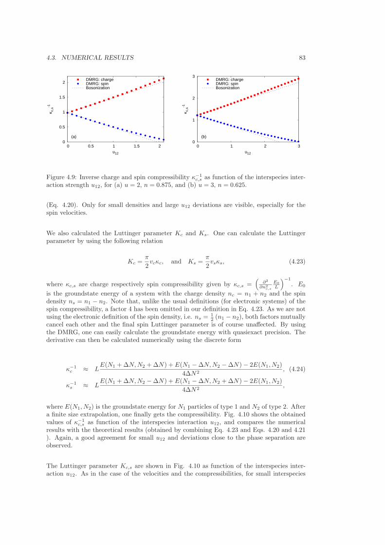
4.3. NUMERICAL RESULTS 83
0
0.5
1
1.5
2
0 0.5 1 1.5 2
κ c,s
-1
u12
(a)
DMRG: chargeDMRG: spinBosonization
0
1
2
3
0 1 2 3
κ c,s
-1
u12
(b)
DMRG: chargeDMRG: spinBosonization
Figure 4.9: Inverse charge and spin compressibility κ−1c,s as function of the interspecies inter-
action strength u12, for (a) u = 2, n = 0.875, and (b) u = 3, n = 0.625.
(Eq. 4.20). Only for small densities and large u12 deviations are visible, especially for thespin velocities.
We also calculated the Luttinger parameter Kc and Ks. One can calculate the Luttingerparameter by using the following relation
Kc =π
2vcκc, and Ks =
π
2vsκs, (4.23)
where κc,s are charge respectively spin compressibility given by κc,s =(
∂2
∂n2c,s
E0
L
)−1
. E0
is the groundstate energy of a system with the charge density nc = n1 + n2 and the spindensity ns = n1 − n2. Note that, unlike the usual definitions (for electronic systems) of thespin compressibility, a factor 4 has been omitted in our definition in Eq. 4.23. As we are notusing the electronic definition of the spin density, i.e. ns = 1
2 (n1 − n2), both factors mutuallycancel each other and the final spin Luttinger parameter is of course unaffected. By usingthe DMRG, one can easily calculate the groundstate energy with quasiexact precision. Thederivative can then be calculated numerically using the discrete form
κ−1c ≈ L
E(N1 + ∆N,N2 + ∆N) + E(N1 − ∆N,N2 − ∆N) − 2E(N1, N2)
4∆N2, (4.24)
κ−1s ≈ L
E(N1 + ∆N,N2 − ∆N) + E(N1 − ∆N,N2 + ∆N) − 2E(N1, N2)
4∆N2,
where E(N1, N2) is the groundstate energy for N1 particles of type 1 and N2 of type 2. Aftera finite size extrapolation, one finally gets the compressibility. Fig. 4.10 shows the obtainedvalues of κ−1
c,s as function of the interspecies interaction u12, and compares the numericalresults with the theoretical results (obtained by combining Eq. 4.23 and Eqs. 4.20 and 4.21). Again, a good agreement for small u12 and deviations close to the phase separation areobserved.
The Luttinger parameter Kc,s are shown in Fig. 4.10 as function of the interspecies inter-action u12. As in the case of the velocities and the compressibilities, for small interspecies

84 CHAPTER 4. BOSONIC SPIN CHARGE SEPARATION
0
2
4
6
8
0 0.5 1 1.5 2
Kc,
s
u12
(a)
DMRG: chargeDMRG: spin
Bosonization
0
2
4
6
0 1 2 3
Kc,
s
u12
(b)
DMRG: chargeDMRG: spin
Bosonization
Figure 4.10: Charge and spin Luttinger parameter Kc,s as function of the interspecies inter-action strength u12, for (a) u = 2, n = 0.875, and (b) u = 3, n = 0.625. The Bosonizationresult is given by Eq. 4.21.
0
2
4
6
8
0 0.25 0.5 0.75 1
Kc,
s
n
u12 = 1.2, chargeu12 = 1.2, spinu12 = 2.7, chargeu12 = 2.7, spinBosonization
Figure 4.11: Charge and spin Luttinger parameter Kc,s as function of the density n for u = 3.

4.3. NUMERICAL RESULTS 85
interaction the agreement is good, while especially the spin Luttinger parameter shows sig-nificant deviations starting at rather small values of u12. Fig. 4.11 shows the Luttingerparameter as function of the density n. Here, stronger deviations are visible, which increasewith increasing density. A similar effect can be observed for an one-component Bose-Hubbardmodel, where for densities above n ∼ 0.5 significant lattice effects can be observed, as previ-ously discussed in section 4.2.1.
In this section, we calculated numerical values for the Bosonization parameter vc,s and Kc,s.In section 4.2.2, we performed a Bosonization analysis of the two-component Bose-Hubbardmodel, where we started from an effective description of both component in terms of aLuttinger liquid. While one also can obtain the single component parameter, v0 and K0, byusing a Bosonization analysis or by comparison with the Lieb-Liniger solution (as discussedin section 4.2.1), the accuracy of Eqs. 4.20 & 4.21 increases significantly if both v0 andK0 are determined numerically. As expected, for small interspecies interactions u12 bothresults fit well, with increasing the interaction u12 the deviations also increase. Only for thespin parameters close to the phase separation significant deviations can be observed. In allother cases we can conclude that using the Bosonization result, Eqs. 4.20 & 4.21, providesan accurate description of both the velocities and the Luttinger parameter, as long as oneobtains the single-component parameter numerically.
4.3.2 Single Particle Excitations
Now we want to consider single particle excitations, as this correspond to the proposed ex-perimental setup. The Bosonization analysis of section 4.2.2 is only valid for low energyexcitations. Hence to test whether the spin-charge separation can be observed by using sin-gle particle excitations, a numerical treatment is necessary.
The time-evolution of single particle excitations of the groundstate is calculated. First, thegroundstate |gs〉 is generated by using the DMRG, then a bosonic creation or annihilation
operator is applied. The initial state is thus |ψ(t = 0)〉 = b†L/2,1 |gs〉. As in the last section, we
also used a Krylov subspace based algorithm to calculate the evolution, but here the numberof states needed is significantly higher. For the results presented in this section, up to 7500states were used.
Fig. 4.12 shows the densities at different times t, for n1 = n2 = 0.625, u = 3, u12 = 2.1,and after applying both b†L/2,1 and bL/2,1. In both cases, the excitation splits first into two
counterpropagating density waves, a left-moving and a right-moving one. Further spin andcharge excitations separate, and are moving with different velocities. Thus, the proposed(section 4.2.2) and for low-energy excitations observed (section 4.3.1) spin-charge separationcan also be seen when considering single particle excitations. The spin-charge separation is arobust effect, even visible for excitations energies beyond the low-energy regime. Therefore,it should be possible to observe this effect by using ultracold atomic gases, as discussed insection 4.1.
In Fig. 4.12 we also plotted the entanglement entropy. When comparing both the evolutionafter applying a creation b† and a annihilation operator b, one can see a substantial differencebetween both cases. For the creation operator, a strong increase in the entropy in the middleof the system can be observed, while for the annihilation operator the entropy does not

86 CHAPTER 4. BOSONIC SPIN CHARGE SEPARATION
0
0.5
1
0 8 16 24 32
1.5
2
2.5
3
n S
site
(a)Entropy
nc - 1.25ns
-0.6
-0.4
-0.2
0
0.2
0 8 16 24 32
1.5
2
2.5
n S
site
(d)Entropy
nc - 1.25ns
-0.2
0
0.2
0.4
0.6
0 8 16 24 32
1.5
2
2.5
3
n S
site
(b)Entropy
nc - 1.25ns
-0.3
-0.2
-0.1
0
0.1
0 8 16 24 32
1.5
2
2.5
n S
site
(e)Entropy
nc - 1.25ns
-0.2
0
0.2
0.4
0.6
0 8 16 24 32
1.5
2
2.5
3
n S
site
(c)Entropy
nc - 1.25ns
-0.3
-0.2
-0.1
0
0.1
0 8 16 24 32
1.5
2
2.5
n S
site
(f)Entropy
nc - 1.25ns
Figure 4.12: Time evolution of the densities after a single particle excitation at t = 0. Thecharge density is shifted by 1.25 for better visibility. The parameters used were L = 32,n = 0.625, u = 3, and u12 = 2.1. (a) - (c) shows the densities after applying the creation
operator b† and at the following times (a) t = 0, (b) t = 1.5, and (c) t = 2.5, (d) - (f) after
applying an annihilation operator b and at (d) t = 0, (e) t = 1.5, and (f) t = 2.5. Onecan clearly see a separation of spin and charge excitations. Additionally, the entanglemententropy of the system is also plotted. Note the big difference of the evolution of the entropyfor the two different cases (b† and b).

4.3. NUMERICAL RESULTS 87
change much (besides some small fluctuations). This interesting effect will be discussed inmore detail in section 4.3.4.
4.3.3 Spectral Functions
In this section, dynamical spectral functions of the two-component Bose-Hubbard model arecalculated. The Green’s function G(z) for an operator A can be defined as
G(z) = 〈gs| A† 1
z + E0 − HA |gs〉 . (4.25)
and the dynamical spectral function as limit
A(ω) = − 1
πIm lim
ηց0G(ω + iη). (4.26)
Section 2.5 deals with the calculation of spectral functions by using matrix product statesin great detail. Here, the GMRES algorithm (section 2.5.2) is used, for L = 64 and η = 0.1approximately 2000 states are needed for the correction vectors.
As usual, MPS algorithms are performing much better for open boundary conditions thanfor periodic boundary conditions. One drawback of open boundary conditions are strongerfinite size effects. In order to reduce the finite size effects, the quasimomentum definition ofthe Fourier transform can be used. The usual Fourier transform can be defined by using theeigenstates of a non-interacting system with periodic boundary conditions. An alternativetransform can be obtained by considering the eigenstates of the non-interacting system, butnow including the open boundaries. Then the transform is given by
bq,ν =
√
2
L + 1
∑
j
sin
(qjπ
L + 1
)
bj,ν , (4.27)
with the momenta |k| = qπL+1 . These eigenstates have nodes at the edges of the system, and
therefore the finite effects are smaller than when the usual Fourier transform is used. In thissection, we only calculate the single particle spectral function, i.e. for b†q.
By using the Bosonization analysis, one can calculate the single particle spectral functionas well. The dispersion relation is linear, ωc,s ≈ vc,sq, where vc,s are the two differentvelocities. Thus one expects divergent peaks at both vc,sq, similar to the single-componentcase discussed in section 4.2.1.
Fig. 4.13 shows the calculated spectral function for u21 = 2.1, u = 3, n = 0.625, L = 64, andη = 0.1. No deconvolution has been performed, and the resulting spectral function has beennormalized for each q, so
∫Aq(ω+ iη) dω = 1 holds for all q and η. For q < 0.25, the spectral
function is not plotted, there finite size effects dominate and would distract attention fromthe physically relevant effects. One can clearly identify both spin and charge excitations.Both branches exhibit a linear dispersion relation for small q up to the order of 1, for biggermomenta effects of the finite band curvature are visible.

88 CHAPTER 4. BOSONIC SPIN CHARGE SEPARATION
Figure 4.13: Density plot of single particle spectral function A(q, ω), u12 = 2.1, u = 3,n = 0.625, η = 0.1, and L = 64. One can clearly identify the linear dispersion relations ofboth charge and spin excitations with different velocities.
0
0.5
1
0 1 2 3 4
A(q
,ω)
ω q-1
k = 10k = 15k = 20k = 25k = 30k = 40
Figure 4.14: Single particle spectral function A(q, ω) for different momenta q ≡ qπL+1 as
function of ωq−1. The two vertical lines correspond the spin and respective charge velocities.The used system parameters are u12 = 2.1, u = 3, n = 0.625, η = 0.1, and L = 64.

4.3. NUMERICAL RESULTS 89
A more detailed view of the spectral function is given in Fig. 4.14, where the spectral functionAq(ω+iη) is plotted as function of w/q. Due to the linear dispersion relation, one expects twopeaks at vs and at vc. The same system parameters as in Fig. 4.13 have been used. A numberof different finite size effects can be observed. For small momenta q, an additional peak atω ≈ 0 appears. Further the peaks are shifted to smaller frequencies, and additional shouldersabove the peak are visible, for instance see the k = 10 spectral function of Fig. 4.14. Similarfinite size effects can be seen in the single-component case, as discussed in section 4.2.1. As inthe single case, the strength of the finite size effects decreases when increasing the momenta q.
Finally, one can also observe effects of the non-vanishing band curvature, which yields a shiftof the peaks to higher frequencies with increasing momenta, as the dispersion relations startsto exhibit deviations from the linear relation. Another interesting effect is the splitting of thecharge peak for high momenta. A similar effect can be seen in the single-component case.The Bethe ansatz solution predicts two different branches. In section 4.2.1, this effect hasbeen shown by a spectral density plot of the Bose-Hubbard model, see Fig. 4.3.
To conclude this section, let us summarize our numerical results. The single particle spectralfunction also shows a clear spin charge separation. Further, one can observe a linear dispersionrelation, even up to considerable big momenta, so the low-energy physics is well describedby a two-component Luttinger liquid (TL2).
4.3.4 Entropy of Entanglement
Entanglement is a key quantity to describe a quantum system. For the algorithm discussedin this thesis, the entanglement entropy acts as main measurement of the complexity of thenumerical treatment. The number of states needed to accurately represent a state of theHilbert space by a matrix product state is roughly proportional to the exponential of theentropy.
In this chapter, we calculate the time-evolution for different setups. In general, by usingthe Lieb-Robinson bound [125], one can show that increase of the entanglement entropy withincreasing time has an upper bound, which is a linear function of the time, [126]. For a globalquench, i.e. a sudden change of the global Hamiltonian, a linear growth can be observed,[127–129]. In contrast, when the quench is only local, i.e. the Hamiltonian is only changedat one position, one observes a logarithmic growth, [130–132].
All setups considered in this chapter are only local quenches, so one can expect a logarithmicincrease for all cases. However, significant differences occur for the different setups. Let usstart with considering small density perturbations, which are used in section 4.3.1 to calcu-late the velocities. Fig. 4.15 shows the time-evolution of a small density perturbation. Theentanglement entropy is basically constant with respect to the time. The perturbation isonly weak, and moves the initial state only slightly away from the groundstate. Hence, theentanglement does not change with respect to time.
This is different when single particle excitations are considered, as done in section 4.3.2. Fig.4.12 shows the time-evolution after a single particle excitation. Applying a creation operatoryields a strong increase in the entanglement entropy, while a destruction operator yields an

90 CHAPTER 4. BOSONIC SPIN CHARGE SEPARATION
2.2
2.3
2.4
8 16 24S
site
1.26
1.28
1.3
n c
t = 0t = 2t = 4
Figure 4.15: Time evolution of the entanglement entropy after a small density perturbation.(u12 = 2.1, u = 3, n = 0.625, and L = 32.)
2.4
2.6
2.8
3
3.2
0 1 2 3
S
t
single particle excitation (b)single particle excitation (b+)small density perturbationgroundstate
Figure 4.16: Time-evolution of the entanglement entropy after single particle excitationsand small density perturbations. Note the enormous difference between the evolution afterapplying a creation and an annihilation operator. The system parameters are u12 = 2.1,u = 3, n = 0.625, and L = 32.
almost constant entropy. To illustrate this effect, the entropy (measured at the middle of thesystem) is plotted as function of the time in Fig. 4.16.
Although the Bose-Hubbard model does not possess any particle-hole symmetry, the differ-ence between the two cases is remarkable. Fig. 4.17 shows the time-evolution of the entropyafter single particle excitations of a single-component Bose-Hubbard model, where one canobserve a qualitatively similar effect.
4.3.5 Experimental Constraints
Up to now, only the case of symmetric intraspecies interaction has been considered. Thetwo species of the Bose-Hubbard model are realized by different hyperfine states of 87Rb.Since the s-wave scattering lengths differ for the two species, one get different intraspeciesinteraction strengths. Having non-equal intraspecies strength couples the spin and the chargesector, hence the spin-charge separation might be destroyed.

4.4. CONCLUSION 91
1
1.2
1.4
1.6
1.8
2
0 1 2 3
S
t
single particle excitation (b)single particle excitation (b+)
Figure 4.17: Time-evolution of the entanglement entropy after single particle excitations fora single-component Bose-Hubbard model, U = 3, n = 0.625, L = 32.
In our setup, the intraspecies scattering lengths are approximately given by a1 = 100.4aB
and a2 = 91.28aB , where aB is the Bohr radius. The interspecies s-wave scattering lengthcan be tuned by a Feshbach resonance. In the following we choose a12 = 80aB and a latticedepth of V0 = 4.3ER, where ER is the recoil energy of the optical lattice. This yields thefollowing Bose-Hubbard parameter, U1/J = 2.983, U2/J = 2.712, and U12/J = 2.377, whichdescribe the experimental setup more accurately.
Fig. 4.18 shows the time-evolution of the densities after a single particle excitation, wherethe system parameter are chosen as just discussed, i.e. with unequal intraspecies interactionstrength. One can still observe a separation of both excitations, so even a small mismatch ofthe interspecies interactions does not destroy the spin charge separation.
Finally, the ultracold atoms have to be confined by a trapping potential, which is heremodelled by a change of the local chemical potential, i.e. εj,ν = ε0(j − j0)
2. Fig. 4.19 showsthe time-evolution of single particle excitations for a system with a trap. Again, the spincharge separation can still be observed.
4.4 Conclusion
The spin-charge separation is a key feature of interacting one-dimensional systems. Up tonow, an experimental test of the separation is a difficult task, only a few experiments haveseen signs of it, [91]. In this chapter, an experimental setup was proposed where it should inprinciple be possible to observe the separation of spin and charge excitations.
Bosonic ultracold atomic gases inside an optical lattice are well described by a BosonicHubbard model. Using two different hyperfine states of the trapped gas, one can realize atwo-component Bose-Hubbard model. This model is known to exhibit a spin-charge separa-tion. It is possible to create single particle excitations in the experiment. By using localizeddensity measurement, one can follow the time-evolution of these excitations, for which thespin-charge separation should also be visible.

92 CHAPTER 4. BOSONIC SPIN CHARGE SEPARATION
0
0.5
1
0 8 16 24 32
site
(a) nc - 1.25ns
-0.2
0
0.2
0.4
0.6
0 8 16 24 32
site
(b) nc - 1.25ns
-0.2
0
0.2
0.4
0.6
0 8 16 24 32
site
(c) nc - 1.25ns
Figure 4.18: Time-evolution of the density after single-particle excitations with realisticparameters, U1/J = 2.983, U2/J = 2.712, U12/J = 2.377, and n = 0.625. The chargedensity is shifted by 1.25 for better visibility.

4.4. CONCLUSION 93
-0.4
0
0.4
0.8
1.2
0 8 16 24 32
n
site
(a)nc - 1.25
ns
-0.4
0
0 8 16 24 32n
site
(d)nc - 1.25
ns
-0.4
0
0.4
0 8 16 24 32
n
site
(b)nc - 1.25
ns
-0.4
0
0 8 16 24 32
n
site
(e)nc - 1.25
ns
-0.4
0
0.4
0 8 16 24 32
n
site
(c)nc - 1.25
ns
-0.4
0
0 8 16 24 32
n
site
(f)nc - 1.25
ns
Figure 4.19: Time evolution of the densities after a single particle excitation at t = 0 with anexternal trapping potential. The charge density is shifted by 1.25 for better visibility. Theparameter used were L = 32, n = 0.625, u = 3, and u12 = 2.1. (a) - (c) shows the densities
after applying of a creation operator b† and at the following times (a) t = 0, (b) t = 1.5, and
(c) t = 2.5, (d) - (f) after applying an annihilation operator b and at (d) t = 0, (e) t = 1.5,and (f) t = 2.5. Again one can clearly see a separation of spin and charge excitations.

94 CHAPTER 4. BOSONIC SPIN CHARGE SEPARATION
In this chapter, it was shown that the spin-charge separation can indeed be observed by theproposed experimental setup. A number of possible complications were discussed. First,both intra- and interspecies scattering lengths are of the same order of magnitude. As soonas the interspecies interaction becomes larger than the intraspecies one, a phase separation ofthe two different species occurs. Hence the experiment is always in the vicinity of the phaseseparation. This limits the Bosonization analysis, which is only valid for small interspeciesinteractions. Our result indicates that even close to the phase separation, the low energyphysics is well described by a two-component Luttinger liquid. A further problem is stemsfrom the considered type of excitation in the experiment. A single particle excitation is not alow-energy perturbation, so it is difficult to use the Bosonization results in this regime. How-ever, the numerical treatment shows that, even beyond the low-energy limit, the spin-chargeseparation can be observed.
Finally, two further experimental complications were considered. The intraspecies scatteringlengths of the two hyperfine states are not equal, yielding non-equal intraspecies interactions.This introduces a coupling between the spin and the charge sector, but it turned out, thatthe spin-charge separation is not destroyed by this coupling. The effects of the trap were alsoconsidered. Again, the spin-charge separation can also be seen with a trap.
The spin-charge separation should be visible in the proposed experimental setup, as it is arobust effect of a two-component Bose-Hubbard model with realistic parameter.

Chapter 5
Dynamical Mean-Field Theory
5.1 Introduction
In this chapter, we want to consider the dynamical mean-field theory(DMFT) and use MPS-based algorithms as impurity solver for the DMFT.
As discussed in chapter 2, matrix product states based algorithm only provide an efficienttool for one-dimensional quantum systems, for systems in higher dimensions the approachquickly becomes unfeasible, since an exponentially large number of states is required to faith-fully represent the states. However, strongly correlated systems in higher dimensions are aninteresting problem. The most prominent example is high-Tc superconductivity, for which itis assumed that it can be described by a two-dimensional Hubbard model. Up to now, dealingwith a two-dimensional Hubbard model is still a difficult problem, no reliable methods areknown to simulate sufficient large systems.
The dynamical mean-field theory [18, 133, 134] (especially its cluster extensions) is maybethe most promising candidate to give an approximation that captures the essential featuresof a two-dimensional Hubbard model. Mean-field theories usually neglect all kind of fluctua-tions in the system. For a number of models, mean-field approximations yield useful results,however, for strongly correlated quantum systems, quantum fluctuations play an essentialrole in the physics of these systems. It is possible to extend the mean-field approach tohandle also local quantum fluctuations exactly, while still neglecting all kinds of spatial ones.This approach is known as dynamical mean-field theory, and will be discussed in this chapter.
Let us now start with discussing classical mean-field theories. Consider a classical Ising modelin a field, given by the following Hamiltonian
H = −∑
ij
JijSiSj − h∑
i
Si, (5.1)
where Si are the Ising spin variables, Si = ±1.
95
96 CHAPTER 5. DYNAMICAL MEAN-FIELD THEORY
We now want to construct a mean-field theory for this model. Consider a single site, theimpurity site S0. By neglecting fluctuations, i.e. (Si − 〈Si〉), for all other sites except theimpurity, one can obtain effective Hamiltonian
Heff = −heffS0, (5.2)
which only acts on the impurity site. heff is an effective field given by
heff = h +∑
i
Ji0 〈Si〉 = h + zJm. (5.3)
z denotes the lattice coordination number. Due to the translational symmetry one cannow conclude that 〈Si〉 is equal for all sites; thus define m ≡ 〈Si〉. The partition functionof the effective Hamiltonian can easily be calculated, yielding the expectation value of themagnetization
m = 〈S0〉Heff= tanh (βh + βzJm) . (5.4)
The magnetization can now be calculated by solving this equation self-consistently.
In the next section it will be shown that this mean-field treatment will be become exactin the limit of infinite dimensions. However, for finite dimensions, it still yields the correctphase diagram and order of the phase transition, but the critical exponents are incorrect.
The mean-field approach neglects any kind of fluctuations. While for a classical model onlyspatial fluctuations are present, quantum models also exhibits another type of fluctuations,quantum fluctuations. This simple mean-field approach, however, cannot take these quantumfluctuations into account. Especially for strongly-correlated systems, quantum fluctuationsplay a crucial role in the understanding of these systems. It is possible to set up a mean-fieldtheory which takes local quantum fluctuations into account, the dynamical mean-field theory(DMFT).
Quantum fluctuations cannot be represented by a simple static effective field (e.g. like heff asjust considered) in general, thus preventing the use of a simple mean-field theory. Considera single site (i.e. the impurity site) embedded in an effective bath. This bath now needsto be represented by a dynamical Green’s function G0(τ), which needs to have an explicittime/energy dependence, in order to take quantum fluctuations into account. The actioninduced by the bath has now the general form
Seff = S0 +∑
σ
∫ β
0
dτ
∫ β
0
dτ ′ c†0σ(τ) G−10 (τ − τ ′) c0σ(τ ′). (5.5)
The magnetization of the mean-field theory, i.e. m = 〈S0〉Heff, is now replaced by the local
impurity Green’s function G(τ −τ ′) =⟨
T c†0,σ(τ) c0,σ(τ ′)⟩
Seff
. Similar to the classical mean-
field theory, the bath Green’s function G0(τ) and the impurity Green’s function G(τ) needs tofulfil a self-consistency equation. The precise form of this equation and a detailed derivationof the DMFT method will be presented in the next section.

5.2. DYNAMICAL MEAN FIELD THEORY 97
Figure 5.1: The Cavity method. The system is split into three parts, the impurity (blue),the bonds connecting the impurity with rest of the system (red), and the rest of the system,the cavity (depicted in black).
5.2 Dynamical Mean Field Theory
5.2.1 Derivation of the DMFT Equations
We would like to start this section with a derivation of the dynamical mean-field theory. Inthe introduction a simple mean-field theory of an Ising model was considered. It is useful toreconsider this approach in order to introduce the so-called cavity method, which can simplybe generalized to the quantum case including quantum fluctuations.
Let us start with considering a single impurity site, similar to the scheme discussed in theintroduction. We want to obtain an effective single-site Hamiltonian. In principle, theeffective Hamiltonian can be calculated exactly by integrating out all other sites,
∑
Si, i 6=0
e−βH ≡ e−βHeff , (5.6)
yielding the effective Hamiltonian which only acts on the single site. The cavity methodprovides an elegant scheme to calculate the effective Hamiltonian. As depicted in Fig. 5.1,one splits the system into three different parts, firstly the impurity site, secondly all bondconnecting the impurity with the rest of the system, and finally the rest of the system, theso-called cavity. This scheme splits the Hamiltonian into three parts, the local part actingonly on the impurity site, H0, the interaction between the impurity and the cavity ∆H, andHamiltonian of the cavity, H(c),
H = H0 + ∆H + H(c). (5.7)
For the Ising model the local part is simply given by H0 = −hS0 and the interaction partby ∆H = −
∑
i Ji0S0Si. The key concept of the cavity method is to perform now a seriesexpansion in the interaction term ∆H to obtain the effective impurity Hamiltonian. Theseries expansion is given by
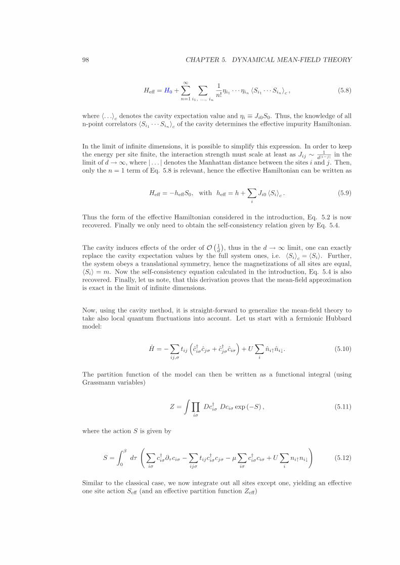
98 CHAPTER 5. DYNAMICAL MEAN-FIELD THEORY
Heff = H0 +∞∑
n=1
∑
i1, ..., in
1
n!ηi1 · · · ηin
〈Si1 · · ·Sin〉c , (5.8)
where 〈. . .〉c denotes the cavity expectation value and ηi ≡ Ji0S0. Thus, the knowledge of alln-point correlators 〈Si1 · · ·Sin
〉c of the cavity determines the effective impurity Hamiltonian.
In the limit of infinite dimensions, it is possible to simplify this expression. In order to keepthe energy per site finite, the interaction strength must scale at least as Jij ∼ 1
d|i−j| in thelimit of d → ∞, where | . . . | denotes the Manhattan distance between the sites i and j. Then,only the n = 1 term of Eq. 5.8 is relevant, hence the effective Hamiltonian can be written as
Heff = −heffS0, with heff = h +∑
i
Ji0 〈Si〉c . (5.9)
Thus the form of the effective Hamiltonian considered in the introduction, Eq. 5.2 is nowrecovered. Finally we only need to obtain the self-consistency relation given by Eq. 5.4.
The cavity induces effects of the order of O(
1d
), thus in the d → ∞ limit, one can exactly
replace the cavity expectation values by the full system ones, i.e. 〈Si〉c = 〈Si〉. Further,the system obeys a translational symmetry, hence the magnetizations of all sites are equal,〈Si〉 = m. Now the self-consistency equation calculated in the introduction, Eq. 5.4 is alsorecovered. Finally, let us note, that this derivation proves that the mean-field approximationis exact in the limit of infinite dimensions.
Now, using the cavity method, it is straight-forward to generalize the mean-field theory totake also local quantum fluctuations into account. Let us start with a fermionic Hubbardmodel:
H = −∑
ij,σ
tij
(
c†iσ cjσ + c†jσ ciσ
)
+ U∑
i
ni↑ni↓. (5.10)
The partition function of the model can then be written as a functional integral (usingGrassmann variables)
Z =
∫∏
iσ
Dc†iσ Dciσ exp (−S) , (5.11)
where the action S is given by
S =
∫ β
0
dτ
(∑
iσ
c†iσ∂τ ciσ −∑
ijσ
tijc†iσcjσ − µ
∑
iσ
c†iσciσ + U∑
i
ni↑ni↓
)
(5.12)
Similar to the classical case, we now integrate out all sites except one, yielding an effectiveone site action Seff (and an effective partition function Zeff)

5.2. DYNAMICAL MEAN FIELD THEORY 99
1
Zeffe−Seff[c
†0σ, c0σ] ≡ 1
Z
∫∏
i6=0,σ
Dc†iσ Dciσe−S (5.13)
Again, we can use the cavity method. The action is split into three parts, one part, S0, onlyacting on the impurity site, another ∆S describing the interaction between the impurity andthe rest of the system, and finally the action for the rest of the system S(c) (cavity).
S0 =
∫ β
0
dτ∑
σ
c†0σ (∂τ − µ) c0σ + Un0↑n0↓ (5.14)
∆S =
∫ β
0
dτ∑
iσ
c†iσ ti0c0σ︸ ︷︷ ︸
≡ηi
+ ti0c†0σ
︸ ︷︷ ︸
≡η†i
ciσ (5.15)
Similar to the classical case (Eq. 5.8), the effective one site action can now be written as aseries expansion in the action ∆S
Seff =
∞∑
n=1
∑
i1,..., in
∑
j1, ..., jn∫
dτi1 · · · dτjnG
(c)i1···in,j1···jn
(τi1 · · · τin, τj1 · · · τjn
)
η†i1
(τi1) · · · η†in
(τin) ηj1(τj1) · · · ηjn
(τjn)
+S0 + const (5.16)
where G(c) denotes the cavity Green’s function given by
G(c)i1···in,j1···jn
(τi1 · · · τin, τj1 · · · τjn
) =⟨
Tc†j1(τj1) · · · c†jn(τj1) ci1(τi1) · · · cin
(τin)⟩
S(c). (5.17)
Consider now again the d → ∞ limit. In order to keep the local energy finite the hopping
needs to scale like tij ∼(
1√d
)|i−j|(where |i − j| is again the Manhattan distance between
the sites i and j.) The only relevant term in Eq. (5.16) is the first term with n = 1. Theeffective action thus has the general form,
Seff = −∫ β
0
dτ
∫ β
0
dτ ′∑
σ
c†0σ(τ)G−10 (τ − τ ′)c0σ(τ ′)
+U
∫ β
0
dτ n0↑(τ) n0↓(τ), (5.18)
with some, at this point arbitrary, Green’s function G0(τ). This Green’s function now takesthe role of the effective Weiss field heff of the classical mean field as discussed in the intro-

100 CHAPTER 5. DYNAMICAL MEAN-FIELD THEORY
Figure 5.2: Sketch of a Bethe lattice with the lattice coordination number z = 3.
duction. However, G0(τ) is not a simple number anymore, in order to take local quantumfluctuations into account G0(τ) needs to be a function of τ . Comparing Eq. (5.16) and Eq.(5.18) yields the self-consistency relation
G−10 (z) = z + µ −
∑
ij
ti0tj0G(c)ij (z), (5.19)
where we used the Fourier transform of the Green’s functions
G(z) =
∫ β
0
dτ exp (zτ) G(τ). (5.20)
Let us now consider a Bethe lattice, as depicted in Fig. 5.2. Due to the lattice geometry,i.e. since S(c) splits the system into z non-connected parts, the non-local Green’s function
G(c)ij (z) is vanishing for i 6= j. As we are considering the limit of infinite lattice dimensions,
the effects induced by considering the cavity construction (instead of the full lattice) areagain of the order O
(1d
). Thus, we can safely replace the cavity Green’s function with the
full impurity Green’s function,
G(c)ii (z) = δijGii(z). (5.21)
Using the translational invariance of the lattice, the local Green’s function Gii(z) is given bythe local Green’s function of the impurity G(z), which enables us to simplify Eq. (5.19),
G−10 (z) = z + µ − D2
4G(z). (5.22)

5.2. DYNAMICAL MEAN FIELD THEORY 101
where we have introduced the bandwidth of the model given by D ≡ 2zt (with z being thelattice coordination number), and
G(τ − τ ′) = −⟨
Tc†0σ(τ)c0σ(τ ′)⟩
Seff
. (5.23)
This defines the self-consistency equations. G0(z) needs to be determined such that the im-purity Green’s function G(z) of the effective action Seff fulfills Eq. 5.22.
Finally, we want to present another derivation of the dynamical mean-field equations whichis not limited to the Bethe lattice. The main ingredient of the dynamical mean-field theoryis that the self-energy function Σ(z) is purely local in space,
Σij(z) = δijΣ(z), (5.24)
or correspondingly, constant in momentum space,
Σ(k, z) = Σ(z). (5.25)
Now we can write down the Dyson equation for the impurity
Σ(z) = G−10 (z) − G−1(z), (5.26)
and express the local lattice Green’s function Gii(z) by the self-energy,
Gii(z) =1
N
∑
k
Gk(z) =1
N
∑
k
(G−1
0 (k, z) − Σ(z))−1
. (5.27)
The non-interacting Green’s function is given by G0(k, z) = (z + µ − εk)−1
, where εk are theenergies of the momentum eigenstates of the non-interacting Hamiltonian. Eq. 5.27 can besimplified by considering the density of states D(z) given by
D(z) =1
N
∑
k
(z − εk)−1
, and its inverse, R[D(ξ)] = ξ. (5.28)
The self-energy of the lattice is now given by
Σ(z) = z + µ − R[Gii(z)]. (5.29)
Finally, by comparing Eq. 5.29 and 5.26, and since the impurity Green’s function G(z) shallbe equal to the (local) lattice Green’s function Gii(z), we obtain the self-consistency equation
G−10 (z) = z + µ + G−1(z) − R [G(z)] . (5.30)
This completes the DMFT algorithm. A general lattice model (given by Eq. 5.10) is mappedto an impurity model, described by the action Seff, for which the self-consistency condition

102 CHAPTER 5. DYNAMICAL MEAN-FIELD THEORY
Eq. 5.30 needs to be fulfilled.
The density of states of a Bethe lattice is semicircular, i.e. given by D(z) =√
D2
4 − z2. Now,
one can calculate R[x] for a Bethe lattice, yielding R[x] = x−1 + D2
4 x. Using this result, Eq.5.30 yields the same self-consistency relation as the one discussed before, Eq. 5.22.
The dynamical mean-field theory approach neglects spatial fluctuations while keeping the fulllocal (quantum) fluctuations. Like the classical mean-field, the DMFT also becomes exactin the limit of infinite dimensions. For vanishing onsite interaction strength, i.e. U = 0, theself-energy Σ(z) vanishes. This simplifies the DMFT, the solution is now given by the non-interacting Green’s function, G0(z) = D(z + µ), which is the exact solution. DMFT is alsoexact in the opposite limit, U → ∞. In this limit the hopping can be neglected, thus εk = 0for all momenta. One can now show, that in this limit the impurity problem is decoupled1,and the DMFT solution recovers the exact Green’s function.
This result is useful when considering the Hubbard model, as the DMFT is able to recover theexact result in both solvable limits. Hence, both phases, the metallic and the Mott-insulationphase are included on the same footing in this approximation.
5.2.2 Solving the DMFT Equation
Overview
The impurity problem described by the effective action Seff (Eq. 5.18) is still an interact-ing many-body problem, for which no general analytic solution is available. Therefore oneusually relies on numerical methods to calculate the Green’s function G(z) of the effectiveimpurity problem, as defined in Eq. 5.23.
In order to numerically solve the self-consistency condition, Eq. 5.30, one can identify theproblem as a fixed point problem for the Green’s functions G(z). Starting with some initialG(z), one first constructs (using Eq. 5.30) the non-interacting Green’s function of the im-purity, G0. This defines a new impurity problem, Eq. 5.18, for which finally a new Green’sfunction G(z) is calculated. One can repeat this loop until convergence is reached, whichimplies the solution of the DMFT equations.
There are a number of different methods available to solve the impurity problem. Most ofthem use a discretization of the bath at some point of the algorithm, which will be discussedin more detail in the next subsection.
Let us start with the simplest method: an exact (numerical) diagonalization of the impurityproblem. The general impurity problem is mapped to a single impurity Anderson model(SIAM) with a finite bath dimension. As the dimension of the Hilbert space scales exponen-tially in the size of the bath, this method is limited to very small bath sizes, only bath sizes up
1i.e. the hybridization function is given by ∆ ≡ 0.

5.2. DYNAMICAL MEAN FIELD THEORY 103
to the order of 20 sites are feasible. This is a severe limitation of this method, however, the ex-act diagonalization is the method with the greatest flexibility of all considered methods, [135].
The second class of algorithms is based on quantum Monte-Carlo methods. A well-knownmethod is given by the Hirsch-Fye algorithm [137], which performs an expansion of theoperator exponential
exp(
−βH)
=N∏
i=1
exp
(
− β
NH
)
≈N∏
i=1
exp
(
− β
NH0
)
exp
(
− β
NHint
)
, (5.31)
which can now be evaluated using a Monte-Carlo scheme. However, one is always restrictedto a finite stepsize ∆β, and thus the limit ∆β → 0 needs to be considered. A big improvementare the continuous-time quantum Monte-Carlo algorithms, which perform a diagrammaticexpansion of either the self-energy Σ(z), [138], or the Hybridization function ∆(z), [139, 140].Further details can be found in [141, 142].
Quantum Monte-Carlo algorithms have two major drawbacks. First of all, as we are con-sidering fermions [10], the sign problem is always present. However, usually one can reachreasonably low temperatures such that it is possible to obtain useful results. The secondproblem is stemming from the fact that these algorithms only allow to access the imaginaryfrequency Green’s functions, G(iω). While it is possible to close the DMFT loop on theimaginary axis, much more insight is gained by considering the Green’s function on the realfrequency axis, i.e. G(ω + i0+). It is possible to perform an analytical continuation to thereal axis by using a deconvolution (which will be discussed in detail in appendix A), butnumerical condition of this problem is even worse than condition of the deconvolution ofDMRG spectral functions.
By using matrix product state-based algorithms (see chapter 2), it is possible to calculate thespectral function for frequencies close to the real axis such that the analytic continuation issimpler than for the QMC data. The numerical renormalization group (NRG) [28–30] uses alogarithmic bath discretization. This yields an optimal resolution at the fermi edge, allowingto resolve the Kondo effect. However, the resolution is deteriorated for all other frequencies.
Another algorithm able to handle the impurity problem is the density matrix renormalizationgroup (DMRG), as considered in chapter 2. Using the DMRG has a number of advantages.First of all, one is not limited to logarithmic discretizations, in the following we will show thatone can use arbitrary discretization schemes. Further it is possible to calculate the spectralfunction for all frequencies with a fixed broadening, thus enabling us to get a good resolutionindependent of the frequency.
DMFT loop
In the following, we want to to present and discuss an algorithm which allows us to use theDMRG as impurity solver for the DMFT. In this subsection, we consider the general DMFTloop in more detail with a special focus on the DMRG as impurity solver.

104 CHAPTER 5. DYNAMICAL MEAN-FIELD THEORY
DMFT
DM
RG
Bath discretization
Eq. 5.34
Eq. 5.30
∆(z)
G(z) G0(z)
HAM
Figure 5.3: Sketch of the DMFT loop.
First let us note, that there are different options to close the DMFT loop. Since all theGreen’s functions G(z), G0(z), and G0(z), and the hybridization function ∆(z) are analyticalfunctions in the upper halfplane, it is sufficient to know these functions only on either the realaxis, the imaginary axis, or for a fixed broadening η, i.e. for all z = ω+iη (and all frequenciesω), since it is possible to perform an analytical continuation to obtain the complete function.This allows us to close the DMFT loop on arbitrary axes. When using the DMRG as solver,one always needs a finite broadening η due to numerical reasons of the MPS-algorithms (asdiscussed in section 2.5).
The Green’s function G(ω + iη) is first calculated with a finite broadening η. Then, Eq. 5.30gives a new G0(ω + iη), which finally gives a new hybridization function ∆(ω + iη), by usingEq. 5.34. Note, that the loop is closed at finite η. This scheme is sketched in Fig. 5.3.
The DMFT loop is repeated until the Green’s function G(ω + iη) is converged. In order tostabilize the convergence, it is sometimes useful to damp the iteration scheme, i.e. instead ofusing the Green’s function obtained by the i-th step, G(i)(z), as input for the next iteration,one can combine the result of the last and the second last step to get a new input Green’sfunction of the next iteration,
(1 − λ) G(i)(z) + λG(i−1)(z). (5.32)
Mapping to Anderson model
The calculation of the Green’s function defined by Seff is the most time consuming part ofthe DMFT algorithm. Dealing with Seff itself is rather cumbersome, since in general there isno Hamiltonian description possible for this form of action. A convenient way to circumventthis problem is to add some auxiliary fermionic bath sites to the system. When the auxiliarysites are integrated out, the remaining action for the impurity should be the same, but thisprocedure enables us to use a Hamiltonian description.
There are many choices onto which model the impurity problem can be mapped, a commonone is the Anderson model
HAM =∑
lσ
Elnlσ +∑
lσ
Fl
(
a†lσ c0σ + h.c.
)
− µ∑
σ
n0σ + Un0↑n0↓, (5.33)

5.2. DYNAMICAL MEAN FIELD THEORY 105
(a) (b)
Figure 5.4: (a) Anderson model with a star geometry, and (b) the transformation to a Wilsonchain.
with a suitable set of parameters Ei and Fi. The lattice geometry is sketched in Fig. 5.4(a). In order to get a system with the same effective one site action, it is useful to define thehybridization function
∆(z) = z + µ − G−10 (z). (5.34)
This function can easily be calculated for the Anderson model (using the non-interactingimpurity Green’s function) [136],
∆AM (z) =∑
i
F 2i
z − Ei. (5.35)
For a given number of bath sites one minimizes the total difference ‖∆ − ∆AM‖ by optimiz-ing the parameters Ei and Fi.
Now, the parameters Ei and Fi of the Anderson model need to be determined such that‖∆ − ∆AM‖ is minimized. This can be achieved by directly solving the (non-linear) opti-mization problem. However, one can write down a more convenient algorithm. Consider thespectral function D∆(ω) of the hybridization function ∆(z),
∆(z) =
∫
dεD∆(ε)
z − ε. (5.36)
By using the deconvolution algorithms which will be discussed in the appendix A, one cannow get an approximation to the spectral function. One can now discretize the bath, i.e.using a given set of intervals [ωi, ωi+1]. The parameters of the Anderson model (Eq. 5.33)are now given by,
F 2i =
∫ ωi+1
ωi
D∆(ω) dω, (5.37)
Ei = F−2i
∫ ωi+1
ωi
ω D∆(ω) dω. (5.38)

106 CHAPTER 5. DYNAMICAL MEAN-FIELD THEORY
0
0.05
0.1
-2 -1 0 1 2
C∆(
ω+
iη)
ω
L = 59L = 99
L = 199input
Figure 5.5: ∆ of Anderson model (input hybridization obtained from converged result, U/D =2.4, half-filled Bethe lattice, broadening η = 0.05, deconvolution parameter σ = 10−7, resultshown in Fig. 5.9).
Fig. 5.5 shows the hybridization ∆AM (ω + iη) of the Anderson model whose parametersare obtained by the scheme just considered. The input hybridization function ∆(ω + iη)is obtained by a converged DMFT loop for a half-filled Bethe lattice, U/D = 2.4, and thebroadening η = 0.05. The deconvolution inside the loop (in order to map the hybridizationto the Anderson model) is performed by the Jackson filter with the parameter σ = 10−7 (seesection A.2.1 for more details).
The hybridization function of the Anderson model, i.e. ∆AM (ω + iη), is plotted at a finitebroadening η = 0.05 for different bath sizes L. The bath discretization is always linear. ForL = 59 one can observe severe finite bath effects, the difference between the input hybridiza-tion and the hybridization of the AM is big. Thus, for this broadening, a bigger bath size isneeded. L = 99 exhibits only small oscillations, which disappears for L = 199.
This scheme is well-controlled. It is possible to directly assess the quality of the bath dis-cretization by considering both the input hybridization ∆(ω+iη) and the resulting hybridiza-tion of the AM, ∆AM (ω + iη). While the deconvolution problem is in general an ill-posedproblem, i.e. the condition number is diverging and thus even small errors are exponentiallyamplified, considering ‖∆ − ∆AM‖ provides an accurate test of the quality of the discretiza-tion scheme.
Furthermore, one always needs to perform both a deconvolution2 and a bath discretization
2The deconvolution is needed, since otherwise the results are really poor. Even a η = 0.5 loop with amodest deconvolution performs much better than η = 0.05 without deconvolution. Further the computationalcosts for a η = 0.5 loop are only a small fraction of the cost of a η = 0.05 loop. Hence a deconvolution isabsolutely necessary to obtain results as accurate as possible while not wasting computational resources.

5.2. DYNAMICAL MEAN FIELD THEORY 107
inside the loop. Combining both approximations in one step allows a much better control.Finally, let us note that is also possible to minimize ‖∆ − ∆AM‖ (at finite η) directly.
DMRG as impurity solver
When using the DMRG as impurity solver, it is useful to transform the Hamiltonian (5.33) toa one dimensional chain (5.39), as depicted in Fig. 5.4 (b). One way to achieve this is givenby using a Lanczos iteration scheme [44], similar to those used for the bath discretization ofthe NRG algorithm [29], to tridiagonalize the bath Hamiltonian. The Lanczos iteration is alsoused in the groundstate DMRG, section 2.3, and for the Krylov time-evolution algorithm,section 2.4.2. Note that the tridiagonalization scheme is a numerical unstable algorithm. Asimple way to circumvent this problem is to increase the accuracy of the used floating pointnumbers, here a precision of several hundreds decimal places ensures the stability.
H =∑
lσ
εlnlσ +∑
lσ
τl
(
a†lσa†
l+1,σ + h.c.)
+ τ0
(
a†1σ c0σ + h.c.
)
−µ∑
σ
n0σ +Un0↑n0↓. (5.39)
After mapping the star geometry to a Wilson chain, the Anderson model given by Eq. 5.39can now easily be handled by the DMRG. First the groundstate |gs〉 is calculated, then boththe single particle and the hole excitation Green’s functions are calculated.
The calculation of these Green’s functions was discussed in section 2.5, here we are using acorrection vector approach and the GMRES algorithm (described in section 2.5.2). For theDMFT the sum of the impurity particle and the hole branch are needed, i.e.
G(z) = Gc†0(z) + Gc0
(−z). (5.40)
It is important to note that the finite broadening η is required, i.e. the Green’s function isevaluated at z = ω + iη. On the one hand, using a finite η smears out effects of the un-avoidable finite bath size. On the other hand, the condition number of the correction vectorequation (Eq. 2.72) diverges for vanishing η, so using a finite η limits the condition numberof the correction vector method, thus limiting the number of states needed.
Fig. 5.6 shows the obtained spectral functions for different broadenings η. The initial hy-bridization function is the one considered in the last subsection, and is shown in Fig. 5.5.For both values of η, the deconvolution using the Jackson filter is performed, a fixed cutofftc is used such that one can compare both deconvolved results. Both deconvolved functionsare almost equal, proving the stability of the deconvolution algorithm.
Finally, in Fig. 5.7 the dependence of the Green’s function on the size of the bath is analyzed.Even a rather small bath size of L = 39 sites yields remarkably good results, especially whencomparing the finite size behavior of the Green’s function to the one of the hybridizationfunction ∆. L = 99 and L = 199 shows virtually no difference, hence for these bath sizes,the results are basically converged.

108 CHAPTER 5. DYNAMICAL MEAN-FIELD THEORY
0
0.2
0.4
0.6
-3 -2 -1 0 1 2 3
C(ω
)
ω
η = 0.1η = 0.2Cη=0.1Cη=0.2
Figure 5.6: Convolved spectral function Cη(ω) and the deconvolution result C(ω) for differentbroadenings η = 0.1 and η = 0.2. The other parameters are L = 99, tc = 0.02, and thehybridization ∆ the same like as the previous plots.
0
0.2
0.4
0.6
-3 -2 -1 0 1 2 3
C(ω
)
ω
L = 39L = 59L = 99
L = 199
Figure 5.7: L scaling, η = 0.1, tc = 0.02, ∆ like in Fig. 5.5

5.2. DYNAMICAL MEAN FIELD THEORY 109
There are a number of parameters which control the quality of the obtained spectral func-tions. On the one hand, the bath must be reasonably large such that the essential physicsof the system is faithfully represented. In the following, we always choose a reasonable bathsize such that the results are basically converged in the size. On the other hand, the cutoffparameter of the deconvolution, tc, directly controls the resolution of the spectral functions.Note that the required bath size depends on this resolution. The cutoff parameter itself isfunction of the accuracy of the DMRG Green’s function (given by σ) and the broadening η,as discussed in the appendix.
The performance of the MPS-algorithm strongly depends on the broadening. When η isreduced by a factor of two, the number of MPS-states needed to faithfully represent thecorrection vector is roughly doubled (in order to keep the accuracy constant), thus the com-putation costs increases by a factor of 8. However, it is also possible to enhance the resolutionby simply increasing the accuracy of the DMRG data, which can be achieved by increasingthe number of states kept. Thus, finding an optimal broadening is always a tradeoff betweenthe increased resolution on the one hand and the increased computational efforts on the otherhand.
In order to conclude this section let us summarize the used algorithm. Starting with aGreen’s function G(ω + iη), one uses the DMFT self-consistency equation, Eq. 5.30, and thedefinition of the hybridization, Eq. 5.34, to obtain a new hybridization ∆(ω + iη). Now weneed to construct an Anderson model, given by the Hamiltonian HAM defined by Eq. 5.33,whose hybridization function ∆AM (ω + iη) equals to the input function, ∆(ω + iη). Thenew model parameter are then used as input for the DMRG, which finally calculates a newGreen’s function.
Using the DMRG as impurity solver provides a well-controlled algorithm to calculate the im-purity Green’s function. The effective action, Seff, needs to be mapped on a Anderson modelinvolves a discretization of the bath, thus introducing an approximation to the scheme. How-ever, by using the algorithms just considered, these approximations can be well-controlled,yielding a stable scheme to solve the DMFT equations.

110 CHAPTER 5. DYNAMICAL MEAN-FIELD THEORY
5.3 Results
5.3.1 Bethe Lattice
We now want to present a number of numerical results. Let us start with considering theHubbard model on a infinite-dimensional Bethe lattice. As we are considering an infinite-dimensional system, the DMFT becomes exact in this limit. For a Bethe lattice, the self-
consistency equation take the simple form ∆(z) = D2
4 G(z), as discussed in the last section.
Half-Filled
Let us start with a half-filled lattice. As discussed in [145], two phases are present in thismodel. For small onsite interactions U , the system favors a metallic phase, for which thespectral function C(ω) exhibits a finite peak at zero frequency. Fig. 5.8 (a) shows the spectralfunction inside the metallic phase; for this plot the interaction strength is set to U/D = 1. Itcan be shown, that the so-called Luttinger sum rule holds for this phase, which states thatthe value of the spectral function at zero frequency, C(0), is pinned to its non-interactingvalue C0(0), for the Bethe lattice C(0) is thus given by 2/π.
On the other side, for big onsite interactions U , one obtains a Mott-insulator, characterizedby a gap in the onsite spectral function, as shown in Fig. 5.8 (c). Finally, there exists acoexistence region, where both phases occur, shown in Fig. 5.8 (b). Therefore two differentcritical onsite interactions are present in this model, Uc1 and Uc2. Above Uc2 the system isalways in the Mott phase, while below Uc1 one can always observe the metallic phase. Thecoexistence region is given by Uc1 < U < Uc2. The phase boundaries Uc1 and Uc2 can becalculated numerically [143, 146], and are given by Uc1/D ≈ 2.39 and Uc2/D ≈ 2.95.
The spectral functions shown in Fig. 5.8 are converged DMFT results obtained by usingthe DMFT as impurity solver. The broadening is set to η = 0.2, a bath size of L = 99 forthe metallic and L = 100 for the Mott-insulating solutions is used, the deconvolution is per-formed by the Jackson filter with σ = 10−7 (see appendix A for more details), and M = 200MPS-states are used. Both the U/D = 1 and the U/D = 4 are virtually converged in theresolution of the impurity solver (which is controlled by the broadening η and the precision ofthe DMRG spectral function, described by the deconvolution parameter σ). For U/D = 2.4,as shown in Fig. 5.8 (b), the Mott gap of the insulating solution is quite small, but, how-ever, by simply increasing the resolution of the DMRG, it is possible to resolve the gap better.
Let us now consider the metallic solution inside the coexistence region. For all other cases,the spectral functions shown in Fig. 5.8 are basically converged in the resolution of theimpurity solver, however, this is not true for the metallic solution for U/D = 2.4. In [143],additional peaks at the inner Hubbard band edges are reported. Using a broadening η = 0.2and the deconvolution parameter σ = 10−7 is not sufficient to resolve this structure.

5.3. RESULTS 111
0
0.2
0.4
0.6
-4 -2 0 2 4
C(ω
)
ω / D
(a)
0
0.2
0.4
0.6
-4 -2 0 2 4
C(ω
)
ω / D
(b)
metallic phaseMott-insulator
0
0.2
0.4
0.6
-4 -2 0 2 4
C(ω
)
ω / D
(c)
Figure 5.8: Converged DMFT spectral functions for a half-filled Hubbard model on a Bethelattice for different onsite interactions U , (a) U/D = 1, (b) U/D = 2.4, and (c) U/D = 4.For all plots, a broadening of η = 0.2 is used and the deconvolution is performed with theJackson filter with σ = 10−7 as discussed in the appendix. L = 99 bath sites are used forthe metallic and L = 100 for the Mott-insulating solutions.

112 CHAPTER 5. DYNAMICAL MEAN-FIELD THEORY
0
0.2
0.4
0.6
-2 0 2
C(ω
)
ω / D
η = 0.05, L = 199η = 0.1, L = 99η = 0.2, L = 79
Figure 5.9: Converged DMFT spectral functions for a half-filled Hubbard model on a Bethelattice for different bath sizes L and broadenings η. The onsite interaction is given byU/D = 2.4, σ = 10−7, and the system is inside the metallic phase.
In Fig. 5.9, the resolution is subsequently increased in order to able to resolve these “satel-lite” peaks. This can achieved by reducing the broadening η while keeping the deconvolutionparameter σ = 10−7 constant. Note, that the bath size needs to be adjusted appropriately.The required number of states kept increases dramatically with decreasing η. Roughly speak-ing, a decrease of the broadening by a factor of two doubles the needed number of states tofaithfully represent the correction vectors. For η = 0.05, M = 1000 states are used.
Our results strongly supports the findings of [143], with increasing resolution the satellitepeaks are enhanced.
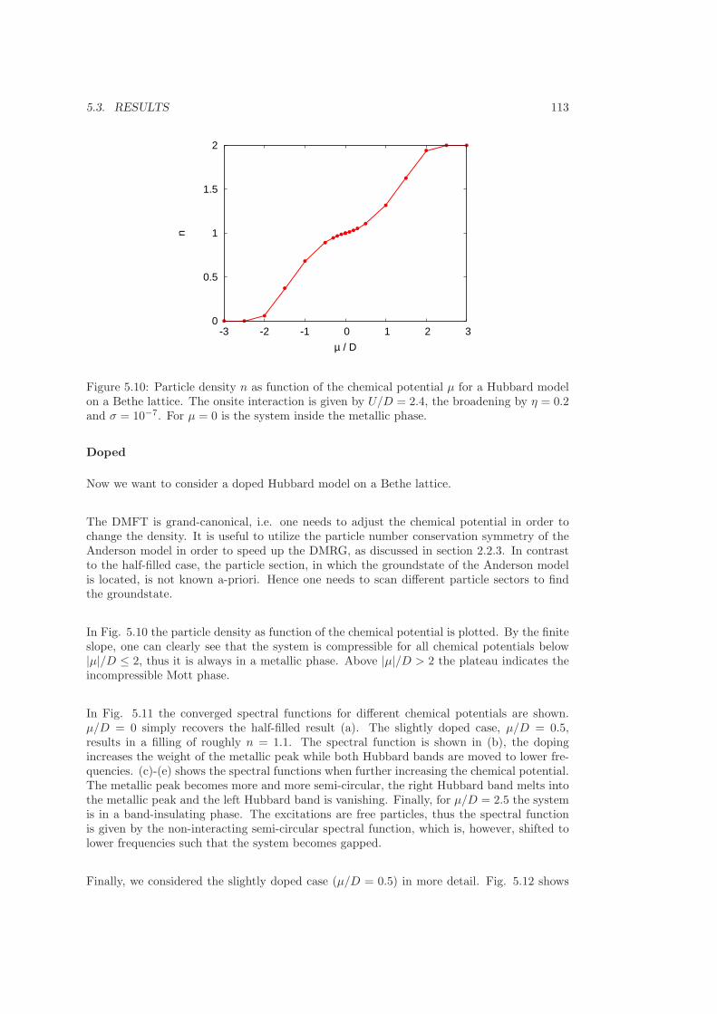
5.3. RESULTS 113
0
0.5
1
1.5
2
-3 -2 -1 0 1 2 3
n
µ / D
Figure 5.10: Particle density n as function of the chemical potential µ for a Hubbard modelon a Bethe lattice. The onsite interaction is given by U/D = 2.4, the broadening by η = 0.2and σ = 10−7. For µ = 0 is the system inside the metallic phase.
Doped
Now we want to consider a doped Hubbard model on a Bethe lattice.
The DMFT is grand-canonical, i.e. one needs to adjust the chemical potential in order tochange the density. It is useful to utilize the particle number conservation symmetry of theAnderson model in order to speed up the DMRG, as discussed in section 2.2.3. In contrastto the half-filled case, the particle section, in which the groundstate of the Anderson modelis located, is not known a-priori. Hence one needs to scan different particle sectors to findthe groundstate.
In Fig. 5.10 the particle density as function of the chemical potential is plotted. By the finiteslope, one can clearly see that the system is compressible for all chemical potentials below|µ|/D ≤ 2, thus it is always in a metallic phase. Above |µ|/D > 2 the plateau indicates theincompressible Mott phase.
In Fig. 5.11 the converged spectral functions for different chemical potentials are shown.µ/D = 0 simply recovers the half-filled result (a). The slightly doped case, µ/D = 0.5,results in a filling of roughly n = 1.1. The spectral function is shown in (b), the dopingincreases the weight of the metallic peak while both Hubbard bands are moved to lower fre-quencies. (c)-(e) shows the spectral functions when further increasing the chemical potential.The metallic peak becomes more and more semi-circular, the right Hubbard band melts intothe metallic peak and the left Hubbard band is vanishing. Finally, for µ/D = 2.5 the systemis in a band-insulating phase. The excitations are free particles, thus the spectral functionis given by the non-interacting semi-circular spectral function, which is, however, shifted tolower frequencies such that the system becomes gapped.
Finally, we considered the slightly doped case (µ/D = 0.5) in more detail. Fig. 5.12 shows

114 CHAPTER 5. DYNAMICAL MEAN-FIELD THEORY
0
0.2
0.4
0.6
-4 -2 0 2
C(ω
)
ω / D
(a)
0
0.2
0.4
0.6
-4 -2 0 2
C(ω
)ω / D
(d)
0
0.2
0.4
0.6
-4 -2 0 2
C(ω
)
ω / D
(b)
0
0.2
0.4
0.6
-4 -2 0 2
C(ω
)
ω / D
(e)
0
0.2
0.4
0.6
-4 -2 0 2
C(ω
)
ω / D
(c)
0
0.2
0.4
0.6
-4 -2 0 2
C(ω
)
ω / D
(f)
Figure 5.11: DMFT spectral functions for a Hubbard model on a Bethe lattice as function ofthe applied chemical potential µ, (a) µ/D = 0, (b) µ/D = 0.5, (c) µ/D = 1, (d) µ/D = 1.5,(e) µ/D = 2, and (f) µ/D = 2.5.

5.3. RESULTS 115
0
0.2
0.4
0.6
-4 -2 0 2
C(ω
)
ω / D
η = 0.1, L = 99η = 0.2, L = 79
Figure 5.12: DMFT spectral functions for a slightly doped Hubbard model on a Bethelattice for different bath sizes L and broadenings η. The system parameter are µ/D = 0.5and U/D = 2.4.
the obtained spectral function for different resolutions. As in the half-filled case, one canclearly observe the satellite peaks.
5.3.2 One-dimensional Hubbard model
Let us now consider a finite dimensional system. Since the DMRG is able to calculate to quasi-exact spectral functions for one-dimensional systems, a one-dimensional half-filled Hubbardmodel is considered. A one-dimensional system is the most difficult case for any mean-fieldtheory, the error induced by considering a finite dimensional system is of the order of O
(d−1
).
The density of the one-dimensional Hubbard model with a bandwidth D is given by
D(z) =(D2 − z2
)− 12 . (5.41)
This result can now be used to calculate R[x], needed in Eq. 5.30 to close the DMFT loop.
In Fig. 5.13 both the quasi-exact spectral functions obtained by the DMRG and the con-verged DMFT results are plotted for different onsite interactions. The one-dimensional Hub-bard model is known to exhibit a Mott phase for any finite interaction strength U , [17].However, the DMFT spectral functions shows significant deviations. Even for onsite inter-actions up to U/D = 3, the DMFT spectral function indicates a metallic phase, as shown inFig. 5.13(a-c). For a small onsite interaction, U/D = 1, the DMFT result agrees, except bythe missing Mott gap, well with the (exact) DMRG spectral function; the DMFT is exactin the non-interacting limit (i.e. U = 0). With increasing U , the deviations become moresevere, however, for U/D = 4, where the Mott-insulating phase is correctly predicted by theDMFT, the deviations starts to become smaller again, as the DMFT is also exact in the

116 CHAPTER 5. DYNAMICAL MEAN-FIELD THEORY
0
0.2
0.4
0.6
0.8
-4 -2 0 2 4
D C
(ω)
ω / D
(a)DMFTDMRG
0
0.2
0.4
0.6
0.8
-4 -2 0 2 4
D C
(ω)
ω / D
(b)DMFTDMRG
0
0.2
0.4
0.6
0.8
-4 -2 0 2 4
D C
(ω)
ω / D
(c)DMFTDMRG
0
0.2
0.4
0.6
0.8
-4 -2 0 2 4D
C(ω
)
ω / D
(d)DMFTDMRG
Figure 5.13: Converged DMFT spectral functions for a half-filled one-dimensional Hubbardmodel with different onsite interactions: (a) U/D = 1, (b) U/D = 2, (c) U/D = 3, and (d)U/D = 4, compared to quasi-exact DMRG spectral functions. The other system parameterare η = 0.2, L = 99, M = 600, and σ = 10−7.
atomic limit (i.e. U → ∞).

5.4. CONCLUSION 117
5.4 Conclusion
Let us now conclude this chapter. The DMRG algorithm has been used as impurity solverfor the dynamical mean-field theory. By using the algorithms considered in section 2.5, it ispossible to calculate the spectral function for real frequencies (and only a small broadeningη), making a physical interpretation of the resulting spectral functions easy. This is a majorconceptual advantage compared to the quantum Monte-Carlo solvers, which are only ableto calculate the Green’s function on the imaginary frequency axis. While it is in princi-ple possible to perform an analytic continuation to obtain the spectral function on the realaxis, the condition of this deconvolution problem is significantly bigger than the conditionnumber of the DMRG deconvolution problem, thus making it numerically even more difficult.
The calculation of the spectral functions by using the GMRES algorithm is the most time-consuming part of the presented algorithm. In order to obtain high-resolution spectral func-tions, big bath sizes on the one hand and small broadenings η on the other hand need to beconsidered. However, this considerably increases the numerical costs. For one iteration witha broadening of η = 0.05 and L = 199 bath sites (for instance as shown in Fig. 5.9), approx-imately a quarter CPU-year on a single-core AMD-K10 is required. It is useful to store thecalculated corrections vectors, they can be used as a starting point for the GMRES algorithmof the next iteration. 500 GB hard-disk space is required to save one set of correction vectors(η = 0.05, L = 199).
The scaling of the required computational time as function of the broadening η is quite bad, adecrease of η by a factor of two doubles the required size of the bath. Additionally, due to thedeteriorated condition number of the correction vector equation (i.e. Eq. 2.72) the numberof needed states is roughly doubled as well. Finally, since the spectral function contains morevisible details, one needs to calculate approximately twice as many correction vectors. So,decreasing the broadening by a factor of two yields a 32-fold (25) increase of the requiredCPU time. Using a broadening of η = 0.025 thus requires 8 CPU-years, η = 0.01 1500 CPU-years per DMFT iteration. The high computational costs substantially limit the usability ofthe DMRG as impurity solver for the DMFT. As discussed in section 5.2.2, continuous-timeQMC algorithms provide efficient solvers which require much less computational resources.
As discussed in section 5.2.1, the errors of the DMFT for finite dimensional systems are givenby O
(1d
). Thus, when considering low-dimensional systems, the DMFT approximation intro-
duces large errors, as observed in section 5.3.2. It is possible to extend the DMFT approach;instead of considering a single impurity site, one can consider a bigger number of sites asimpurity. A review of these cluster extensions can be found in [147].
We have refrained from studying cluster extensions by using the DMRG as impurity solver,as the computational requirements greatly increase for multi-impurity Anderson models. Fora two impurity Anderson model, even for L = 99 bath sites and a (big) broadening of η = 0.2,more than M = 1000 states are needed for the correction vectors, requiring large computa-tional resources.
Again, the computational costs of the DMRG algorithm are significantly higher than forcontinuous-time QMC algorithms. In recent times, these algorithms have successfully beenapplied to two-dimensional Hubbard models, [148–150].

118 CHAPTER 5. DYNAMICAL MEAN-FIELD THEORY
To finally conclude this chapter, we would like to give an outlook. At the present day, theuse of the DMRG algorithm as impurity solver for the dynamical mean-field theory is mainlyrestricted by the limited available computational power. However, according to Moore’s law,the speed of the computing facilities will further be increased. By the end of 2010, the clustersof the Rechenzentrum of RWTH Aachen will provide an accumulative power of 200 TFlops,the 20000-fold of a single core K10. Most of the simulations of this chapter were done on a100 cores in parallel, thus, using the whole extended cluster3 would provide a speedup by afactor of 100, allowing an η = 0.025 iteration to finish within four hours, an η = 0.01 onewithin 25 days.
Another completely different brute-force approach to obtain more computing power is givenby using the GPU (graphics processing unit) of modern video cards. At the moment, thefastest available video cards on the market offer 5 TFlops raw power, the next generationproviding 12 TFlops will be available within this year (by the end of 2010). It is possible toequip a system with up to 8 video cards for less than 10000 e, thus providing approximately100 TFlops with only modest costs.
Finally, let us note that instead of using matrix product states, it is also possible to use othertensor product states. In [151], star-like geometries which employ tensors with higher ranksat the impurity have been considered. This may yield a considerable speedup, and hencemaking cluster extension of the DMFT feasible. In my opinon, it is worthwhile to spendfurther research efforts on this topic, especially regarding cluster extensions of the dynamicalmean-field theory.
3Which is, of course, not possible with the RWTH Rechenzentrums-cluster.

Appendix A
Deconvolution
A.1 Introduction
In section 2.5, the calculation of Green’s functions G(z), z ≡ ω + iη, by using matrix productstates is considered. Physically more interesting is the spectral function D(ω) of a Green’sfunction, which can be related to the Green’s function by a convolution,
G(z) =
∫
dωC(ω)
z − ω. (A.1)
It is also possible to consider only the imaginary part of the Green’s function. Then, theconvolution can be written as
Cη(ω) =
∫
dω′ C(ω′) Lη(ω − ω′), (A.2)
where Lη(ω) = ηπ
1ω2+η2 is a Lorentz function. The deconvolution is a crucial part of the
DMFT, as discussed in chapter 5.
We want to consider different numerical algorithms which can be used to perform a decon-volution of a convolved function. Let us start with considering a general deconvolution. Ageneral convolution of the function f(ω) with a kernel K(ω) is given by
g(ω) =
∫
dω′ f(ω′) K(ω′ − ω). (A.3)
The calculation of g for a given f is rather straight-forward, as one just needs to (numerically)evaluate the integral. There are number of numerical methods available which are able todeal with this problem. However, the inverse case is much more complicated. For a givenfunction g(ω) and a kernel K(ω), one needs to find a function f(ω) such that Eq. A.3 holds.
By using the Fourier transform one can easily write down a solution to this problem. Let usstart with defining the Fourier transform of f(ω) as
119

120 APPENDIX A. DECONVOLUTION
f(t) =
√
1
2π
∫
dω f(ω) eiωt. (A.4)
The convolution becomes diagonal in the time domain,
g(t) =√
2π f(t) K(t). (A.5)
This result is also known as convolution theorem. Now the convolution can easily be inverted,
f(t) =1√2π
g(t)
K(t). (A.6)
Finally we need to transform f(t) back to the frequency domain, i.e.
f(ω) =
√
1
2π
∫
dω f(t) e−iωt. (A.7)
This solves the deconvolution problem in general. However, depending on the kernel K(ω),the condition number of this problem can be very large, even a diverging condition numbercan often be observed, as we will show below, signaling an ill-posed problem.
In order to illustrate this, let us now consider the example of dynamical spectral functions,as just discussed. Due to numerical reasons of MPS algorithms, a finite broadening η isalways needed, and thus the obtained spectral function is broadened by a Lorentzian kernel,K(ω) ≡ Lη(ω). The Fourier transform of this kernel is given by
K(t) = exp (−η|t|) . (A.8)
As we are considering numerical algorithms there are always errors present in the input data,g(ω), for instance induced by the finite floating point precision. This can be interpreted asnoise in the input data, allowing to define a signal-to-noise ratio of g(ω). The SNR (in thetime-domain) of a general noisy function h(ω) is given by
Sh(t) =h(t)2
σh(t)2, (A.9)
where σh(t)2 is variance of the noise (i.e. the squared error of h). When the signal-to-noiseratio is significantly smaller than one, the noise is much stronger than the actual signal, henceit is difficult to obtain the correct underlying signal as the result is dominated by randomnoise. However, if the SNR is much bigger than one, the noise disturbing the signal is muchsmaller than the signal itself, thus it is easy to get the correct signal.
Consider now a noisy input function g(ω) with the SNR Sg(t) and a Lorentzian kernel asinput of the deconvolution problem, Eq. A.3. After performing a simple error propagationanalysis one obtains the signal-to-noise ratio of the result f(ω) which is given by

A.1. INTRODUCTION 121
Sf (t) = Sg(t) exp (−2η|t|) . (A.10)
Even for arbitrary small noise of the input signal g (for instance induced by the finite float-ing point precision), the noise of the output signal diverges for |t| → ∞. Thus any directnumerical solution of deconvolution problem with a Lorentzian kernel will always be spoiledby diverging errors, preventing any solution of this problem. The condition number of theproblem is not finite, hence the problem is ill-posed. However, there are a number of differ-ent approaches available which transform an ill-posed problem into a well-posed one, usuallydone by enforcing additional constraints like the continuity of the solution. This procedureis also known as regularization.
In the following section we want to present a number of different algorithm which regularizethe deconvolution problem, thus make a stable numerical solution possible. We would like tostart with the consideration of a class of algorithms based upon simple linear filters designedto keep the overall signal-to-noise ratio finite, for more details see section A.2.1. The nextapproach is based on statistics, i.e. by maximizing an entropy measure, one can find themost probable solution. This approach will be discussed in section A.2.2. Finally we wantto compare both approaches and draw a conclusion in section A.3.

122 APPENDIX A. DECONVOLUTION
A.2 Methods
A.2.1 Linear Schemes
In this section we want to present two different algorithm which regularize the deconvolutionproblem. In the first subsection simple linear filters are constructed.
Let us first sketch the general algorithm used in this section. First a Fourier transformof the input data function g(ω) is performed. Now we can use Eq. A.6 to obtain thedeconvolved result f(t) in the time-domain. However, due to the bad condition number ofthe deconvolution problem, there might be regions where the signal-to-noise ratio is vanishing,thus introducing arbitrary large errors in the result. By using a linear filter given by C(t) inthe time domain,
f(t) = f(t) · C(t), (A.11)
one can filter out the regions with a bad signal-to-noise ratio. This prevents the amplificationof small errors present in the input data, which would otherwise spoil the result. Finally,we need to perform another Fourier transformation to obtain the final result f(ω). Sincethe input data is usually given on a equidistant grid, it is possible to use a Fast FourierTransform, which scales linear in the number of data points (up to logarithmic corrections),thus allowing a much faster computation of the transform than the simple straight-forwardalgorithms.
In this chapter we only consider Gaussian white noise, this assumption/restriction will bediscussed in more detail in section A.3. Consider now a function fexact. Adding noise yieldsa noisy new function fnoisy with a finite signal-to-noise ration Sf (t). Now we can apply afilter (given by C(t)) to (partially) reconstruct the original function fexact.
fexactnoise−−−→ fnoisy
filter−−−→ freconstructed
In order to assess a filter, one usually considers expectation value of 2-norm of the difference
⟨∥∥∥fexact − freconstructed
∥∥∥
2⟩
. (A.12)
In [152] the so-called Wiener filter is proposed, which minimizes the error given by Eq. A.12.The filter is given by
C(t) =Sf (t)
Sf (t) + 1. (A.13)
For regions where the signal-to-noise ratio is large, the filter is approximately unity, andthus it does not alter the result. However, when the signal-to-noise ratio is small, C(t) isexponentially small, thus these regions in the time domain are suppressed.
By using the convolution theorem one can write down these filter as convolutions in thefrequency space,

A.2. METHODS 123
0
0.5
1
0 1 2
C(t
)
t / tc
(a)
boxWiener
0
0.1
0.2
0.3
-20 -10 0 10 20
C(ω
) / t
c
ω tc
(b) boxWiener
Figure A.1: The Wiener filter (given by Eq. A.15)) and a box filter plotted (a) in the timedomain and (b) in the frequency domain. Note that the Wiener filter does not possess anycutoff frequency. In order to be able to compare both filter tc of the box filter is chosen suchthat for the Wiener filter C(tc) = 1
2 holds.
f(ω) =
∫
dω′ f(ω′) C(ω′ − ω). (A.14)
Consider now a delta function δ(ω) with the signal-to-noise ratio Sδ(t) = S0 exp (−2η|t|).which is a typical SNR after performing deconvolution of a Lorentzian kernel, Eq. A.10, anda constant SNR S0 of initial data (i.e. the convolution of the delta function). Now the filteris given by
C(t) =S0
S0 + exp (2η|t|) . (A.15)
In Fig. A.1 a Wiener filter, given by Eq. A.15, and a simple box filter are plotted as functionof both time and frequency. In the frequency domain both filter exhibit strong oscillations,which is known as the Gibbs phenomenon[153–155], discovered more than hundred years ago.
The only deconvolution problem considered in this thesis is the deconvolution of spectralfunctions (see section 2.5). However, groundstate spectral functions (for zero temperature)do not need to be analytic functions, the Gibbs oscillations will always spoil the deconvolu-tion results.
This problem has been intensively discussed in the beginning of the last century. Nowadaysthere are well-established solutions available. Let us consider filter with a hard cutoff time tc
C(t) =
{
C(
ttc
)
, |t| < tc
0, else(A.16)
A simple box filter is then given by the constant function
Cbox(x) = 1. (A.17)

124 APPENDIX A. DECONVOLUTION
0
0.2
0.4
0.6
0.8
1
0 0.5 1
C(t
)
t / tc
boxFejerJacksonBlackman
Figure A.2: Different linear filter in the time-domain.
As seen in Fig. A.1 (b), the box filter exhibits severe Gibbs oscillations. In [156] Fejerproposed a different filter which removes the first order of the Gibbs oscillations. Instead ofconsidering a box filter, a smooth filter is used, given by
CFejer(x) = 1 − x. (A.18)
Fig. A.2 shows the different considered filter as in the time domain and Fig. A.3 in thefrequency domain. As discussed before, the box filter exhibits a severe Gibbs problem. TheFejer filter significantly reduces the oscillations, however, oscillations with a smaller amplituderemain. It is possible to further suppress theses oscillations. For the Jackson filter [157], givenby
CJackson(x) = (1 − x) cos (πx) +1
πsin (πx) , (A.19)
almost no oscillations are visible anymore. Fig. A.4 shows a log-log plot of the filter inthe frequency domain. Both the Fejer and the Jackson filter are positive in the sense thatC(ω) ≥ 0 holds for all ω. Since C(t = 0) = 1 holds for all the considered filters (exceptthe Wiener filter where this only approximately holds), the filters preserve the norm. Bothproperties are useful when considering dynamical spectral functions, since spectral functionsare usually both positive and normalized.
Besides the positivity there are a number of other points which can be used to assess thequality of a filter. When considering the limit ω → ±∞ the envelop of the oscillations isgiven by a power-law, C(ω) ∼ |ω|−α, with an integer exponent α. For the box filter theexponent is given by α = 1, thus the oscillations are only weakly damped. The Fejer filterhas α = 2, the Jackson α = 4, hence the Gibbs oscillations are much weaker for these filters.

A.2. METHODS 125
0
0.1
0.2
0.3
-20 -10 0 10 20
C(ω
) / t
c
ω tc
boxFejer
JacksonBlackman
Figure A.3: Different linear filter in the frequency-domain.
However, the width of the main lobe, i.e. the peak at zero frequency, becomes smaller for thehigher order filter, thus the resolution is reduced. For the filters with higher orders, i.e. theFejer and the Jackson filter, the most important side lobe besides the main lobe is the secondpeak, its height is effectively measuring the strength of the Gibbs problem (the other peaksare even more damped and thus the first side lobe is the relevant one). One can construct afilter where the first side lobes are suppressed while the resolution is kept comparable to theJackson filter. This filter is the Blackman filter and given by
CBlackman(x) = a0 + a1 cos (πx) + a2 cos (2πx) , (A.20)
with the parameters
a0 =3969
9304≈ 0.42, a1 =
2310
4651≈ 0.50, a2 =
1430
18608≈ 0.08. (A.21)
As one can see in Fig. A.4, the weight of the first four side lobes is much smaller than theone of the Jackson filter. However, the envelope of the tail of the Blackman filter is given byα = 1 (since C(1) 6= 0 for the Blackman filter), thus the Jackson filter is much more localized.Further the Blackman filter is not positive. There are a big number of other filters available,extensive reviews can be found in [158–160].
Let us now summarize the described schemes which regularize the general deconvolutionproblem. Given a (noisy) input function g(ω), first the Fourier transform g(t) is calculatedby using a Fast Fourier Transform (FFT). In the time domain, the (de)convolution becomesdiagonal, thus one can easily perform the deconvolution in the time domain, yielding f(t).Now given the signal to noise ratio of the input data, one can use a error propagation analysisto get the SNR Sf (t). A reasonable choice of the cutoff time tc is the time, where the SNR

126 APPENDIX A. DECONVOLUTION
10-6
10-4
10-2
100
1 10 100
C(ω
) / t
c
ω tc
boxFejer
JacksonBlackman
Figure A.4: Different linear filter in the frequency-domain. The dotted lines represent nega-tive values of C(ω).
drops below 1, i.e. Sf (tc) ≡ 1. Then the discussed filters can be applied in order to improve
the signal to noise ratio of the result. Finally f(ω) is obtained by another FFT. Thus thegeneral algorithm is schematically given by
g(ω)FFT−−−→ g(t)
deconvolution−−−−−−−−−→ f(t)filter−−−→ f(t)
FFT−−−→ f(ω). (A.22)
In order to estimate the SNR of the input data, a useful assumption is that the variance ofthe noise is constant in the frequency domain, i.e. the errors are assumed to be a constant σfor all frequencies. Then the SNR is given by
Sg(t) =|g(t)|2
σ2. (A.23)
By using this SNR one can now obtain the cutoff time tc. Finally we want to present someresults obtained by these algorithms.
The dynamical mean-field theory, as discussed in chapter 5, requires a deconvolution insidethe DMFT loop. Here we want to consider the deconvolution of a converged spectral function.The broadening is given by η = 0.05 and we are considering a half-filled Bethe lattice withU/D = 2.4. The deconvolved spectral function is shown in Fig. 5.9.
Fig. A.5 shows the resulting spectral functions obtained by the Jackson filter with differentvalue of σ. With decreasing σ the cutoff time tc is increased, which increases the resolution.For big σ a number of details of the spectral function are smeared out. When, however, σ istoo small the errors of the initial data becomes visible. In this case σ = 10−7 is a reasonablechoice, while suppressing the error sufficiently the resolution is maximized. Note that no

A.2. METHODS 127
0
0.2
0.4
0.6
-2 0 2
D C
(ω)
ω / D
σ = 10-10
σ = 10-7
σ = 10-3
Cη
Figure A.5: Deconvolution of a converged DMFT/DMRG spectral function using a Jacksonfilter with different σ. The spectral function was calculated for a half-filled Bethe lattice,U/D = 2.4 and by using a broadening of η/D = 0.05, as shown in Fig. 5.9.
Gibbs oscillations are visible.
Finally, we want to consider the effects of the different filters, see A.6. For this data wechoose σ = 10−2 such that basically no noise of the input data is affecting the results. Asexpected, strong Gibbs oscillations are visible when using the box filter. These oscillationscan be reduced by using better filters, which, however, decrease the resolution. For the Fejerfilter one can still observe small oscillations (at ω ≈ 1.1) Both the Jackson and the Blackmanfilter finally remove this oscillation, thus with respect to the Gibbs problem both filter yieldthe best results.
A.2.2 Maximum Entropy Methods
Now, we want to consider a different approach to regularize the deconvolution problem.Based on a statistical analysis, we derive a likelihood of spectral functions solving the de-convolution problem. Then the most probable spectral function is taken as the deconvolvedspectral function. This approach is known as Maximum Entropy Methods(MaxEnt), for anintroduction see [161–163].
A physical spectral function n(ω) fulfills a number of conditions: first, it can be normalized(∫
dω n(ω) = 1) and it is positive (n(ω) ≥ 0), thus it can interpreted as a probability density.
Bayes theory gives us the likelihood of a spectral function n(ω) (without any further knowl-edge about the function) with respect to a so-called default model D(ω) as L1 ∼ exp
(α1S[n]
),
where S is the usual von Neumann entropy,

128 APPENDIX A. DECONVOLUTION
0
0.2
0.4
0.6
0 1 2
D C
(ω)
ω / D
JacksonBlackman
Fejerbox
"exact"
Figure A.6: Plot of the deconvolved spectral function obtained by using different linear filtersfor σ = 10−2. As in Fig. A.5, a DMFT/DMRG spectral function is used as input spectralfunction. The “exact” result is obtained by using a Jackson filter with σ = 10−7.
S[n] = −∫
dω n(ω) log
(n(ω)
D(ω)
)
, (A.24)
and some constant α1 > 0. One can show that S[n] ≤ S[D] = 0, so the most probablespectral function is given by the default model. The default model can be used to includea-priori known information of the result. It is useful not to restrict ourselves to normalizedspectral functions. In this case a reasonable definition of the entropy is given by a generalizedShannon - Jaynes entropy (which simplifies to the usual von Neumann entropy when bothn(ω) and D(ω) share the same norm, see [162]),
S[n] =
∫
dω
(
n(ω) − D(ω) − n(ω) log
(n(ω)
D(ω)
))
. (A.25)
Since we want to find a spectral function n which fulfills the convolution equation, g(ω) =∫
dω′ K(ω − ω′)n(ω′), one can consider the squared norm of the residual of the convolutionwhich is given by
H[n] =
∫
dω1
σ(ω)2
∣∣∣∣g(ω) −
∫
dω′ K(ω − ω′) n(ω′)
∣∣∣∣
2
. (A.26)
where σ(ω) is a measure of the errors of the input function g(ω). Again one can use Bayestheory to obtain a likelihood of a test function n which shall fulfill the convolution equation,namely L2 ∼ exp (−α2H[n]). Combining both L1 and L2 one obtains the most probablespectral function, which on the one hand minimizes the residual of the convolution equation

A.2. METHODS 129
and on the other hand also minimizes the contained information. The overall likelihood isgiven by
L ∼ exp(
− α (H[n] − β−1S[n])︸ ︷︷ ︸
≡F [n]
)
, (A.27)
so the most probable spectral function is the one which minimize the free energy F [n] for agiven parameter β. Consider a variation of the test function n(ω) → n(ω)+ δn(ω). Then thevariation of both H[n] and S[n] can be calculated,
δH[n] = −∫
dω δn(ω)
∫
dω′ K(ω − ω′) A(ω′), (A.28)
δS[n] = −∫
dω δn(ω) logn(ω)
D(ω). (A.29)
where
A(ω) ≡ 2
(
g(ω) −∫
dω′ K(ω − ω′) n(ω′)
)
. (A.30)
We are looking for the spectral function n(ω) which minimizes the free energy F [n]. F [n]is then stationary, i.e. the variation of the free energy is vanishing, δF [n] = 0. Now, sincethis holds for arbitrary variations δn(ω), it is straight-forward to write down the MaxEntequations
n(ω) = D(ω) exp
(
β
∫
dω′ K(ω − ω′) A(ω′)
)
,
A(ω) = 2
(
g(ω) −∫
dω′ K(ω − ω′) n(ω′)
)
, (A.31)
which form a set of non-linear equations. In order to obtain the most probable spectralfunctions, these equations need to be fulfilled self-consistently. As we want to solve theseequation numerically, one needs to discretize them at some point. There are different optionsavailable. Let us start with considering a discretization of n(ω), which is represented as
n(ω) =∑
i
cini(ω), (A.32)
where ni(ω) are some functions forming a basis. Inserted into the MaxEnt equations, Eq.A.31, this yields a set of non-linear equations for the parameter ci. These equations cannow be solved by using a Newton algorithm. However, this discretization scheme exhibits afundamental instability. A prerequisite for the Maximum Entropy approach is the positivityof the test function n(ω). This requirement needs to be additionally imposed here, yieldinga serious loss of stability of the algorithm. This can be prevented by considering anotherdiscretization scheme, which discretizes

130 APPENDIX A. DECONVOLUTION
10-8
10-6
10-4
10-2
100 102 104 106 108 0
0.5
1
1.5
2
H[n
]
-S[n
]
β
H[n]-S[n]
Figure A.7: Energy H[n] and Entropy S[n] of the most probable spectral function as functionof the inverse temperature β.
A(ω) =∑
i
ciAi(ω). (A.33)
We again obtain a set of non-linear equations for the parameter ci, which can be solved by aNewton algorithm. This approach, however, does not have any positivity problems as n(ω)is, per definition, always positive. There exists an elegant derivation of this scheme, whichis based on test functions for the functional H[n]. Consider some functions Ai(ω). Now, wecan reformulate the functional H[n]
H[n] =∑
i
1
σ2i
∫
dω
∣∣∣∣Ai(ω)
(
g(ω) −∫
dω′ K(ω − ω′) n(ω′)
)∣∣∣∣
2
. (A.34)
When the Ai(ω) form a complete orthonormalized basis set of the full Hilbert space thereformulated functional is equal to the original functional H[n] given by equation Eq. A.26.Now one can again perform the derivation of the MaxEnt equations, however, this formula-tion yields directly the discretization scheme given by Eq. A.33. This derivation was firstperformed in [164].
We have considered different ansatz functions Ai(ω). Simple choices are for instance equidis-tant delta peaks, stepfunctions, splines, Wavelets, or Chebyshev polynomials. However, aslong as one considers a reasonable number of ansatz functions, the resulting spectral func-tions do not change (significantly).
The MaxEnt approach has still a free parameter left, the “inverse temperature” β. For smallβ the dominant term in the free energy F [n] is the entropy term, thus the resulting spectralis basically given by the default model. In the limit β → ∞, or correspondingly T → 0,

A.2. METHODS 131
0
0.2
0.4
0.6
0.8
-1 0 1
n(ω
)
ω
β = 104
β = 106
β = 109
exact
Figure A.8: Most probable spectral function n(ω) for different inverse temperatures β.
the dominant term is given by the energy H[n]. Then, the result is the spectral functionwhich minimizes the energy, corresponding to the straight-forward solution considered in thebeginning of this chapter and is thus fully affected by the exponentially large errors.
Now we want to consider a test case, given by a semicircular spectral function,
C(ω) =
{
2π−1√
1 − ω2, for |ω| < 1,0, else.
(A.35)
First, the convolution with a Lorentzian kernel (η = 0.1) is performed, then some noise isadded to the convolved spectral function. The resulting function is then used as input datafor the MaxEnt deconvolution.
Fig. A.7 shows the value of the functional H[n] for the most probable spectral function asfunction of the inverse temperature β. One can distinguish three different regions: for smallβ (maybe up to β ≈ 102) the energy is virtually constant with respect to β. In this region thespectral function is basically given by the default model, for which the entropy is vanishing.This changes when further increasing β. From β ≈ 102 up to β ≈ 2 · 106 the energy andthe entropy are decreasing with increasing β. At both β ≈ 102 and β ≈ 2 · 106, one canobserve a kink in energy H[n]. Beyond the second kink the energy is again a constant. Inthis region, the most probable spectral function is basically the one which minimizes theenergy functional, the entropy term of the free energy is not relevant anymore.
In Fig. A.8 the resulting spectral functions n(ω) for different inverse temperatures are shown.For β = 109 the obtained spectral function exhibits severe artificial oscillations. As in thisparameter region the obtained spectral function minimizes the energy functional, the di-verging condition number of the deconvolution problem reappears, thus small errors of the

132 APPENDIX A. DECONVOLUTION
input data will be exponentially amplified. With decreasing β, the oscillations disappear. Atβ = 106, close to the second kink, the errors vanish. When further decreasing the inversetemperature, the default model D(ω) (here a simple flat spectral function) becomes visible.
Based on this analysis, we can conclude that the optimal inverse temperature is at the secondkink, at the point where the oscillation, due to errors of the input data, are not yet present,while the optimization of the spectral function has carried out best possible.
Finally, we like to mention another similar approach. One can interpret the energy functionH[n] given by Eq. A.26 as the Hamiltonian of a classical field theory with the field n(ω).Now we can calculate the partition function
Z =
∫
Dn exp (−βH[n]) , (A.36)
and the expectation value of the field n(ω) at a finite temperature,
〈n(ω)〉β =1
Z
∫
Dn n(ω) exp (−βH[n]) , (A.37)
where∫
Dn denotes the functional integral over all possible realization of n. The calculationof the expectation values can, in general, not be performed analytically, however, it is possibleto evaluate the integrals by using a Monte Carlo algorithm [165]. Beach has shown in [166],that the maximum entropy approach can be interpreted as mean-field solution of this fieldtheory (with a flat default model). However, we have refrained to study this approach inmore detail, as the needed CPU time to evaluate the functional integrals is large. Even thesimplest problems need more than one day on a 16core AMD-K10 running at 2.3 GHz, whichis considerably more time than for the needed time of the other algorithms1.
1The runtimes are less than one second for the linear schemes and of the order of several minutes for theMaxEnt algorithms on a single core AMD-K10.

A.3. COMPARISON AND CONCLUSION 133
0
0.5
1
-1 -0.5 0 0.5 1
C(ω
)
ω
box filterJackson filterMaxEntexact
Figure A.9: Deconvolution of a box function by using two linear filters, a simple box filterand a Jackson filter, and by the MaxEnt algorithm. The broadening is given by η = 0.1.
A.3 Comparison and Conclusion
In this section we want to compare the different algorithms. Let us start with some generalconsiderations about spectral functions. Usually, the spectral functions obtained by DMRGare for system with zero temperature, thus in general they do not need to be an analyticfunction of the frequency. For instance, a simple band edge yields a discontinuity of the spec-tral function. Further there may be sharp resonances present, represented by delta functions.When the simple linear filters (like a box cutoff filter) are applied to these spectral functions,severe Gibbs oscillations are emerging which dramatically deteriorate the use of these filters.
The situation is considerably different when calculating finite temperature spectral functions.A finite temperature always smears out the spectral function, thus there one only needs toconsider analytic functions which simplifies the deconvolution problem significantly. Whenusing quantum Monte-Carlo algorithms as impurity solver for the DMFT, the simulation willbe performed at a finite temperature (since otherwise the sign problem prevents to get anyuseful results).
In order to assess the quality of the different algorithm, we want to consider the deconvolutionof a box function. First a convolution with a Lorentzian kernel with η = 0.1 is performed, andthen small random errors are added to the convolved spectral function. Now, the differentalgorithms are applied to this problem and the results are compared.
Let us start with considering the MaxEnt deconvolution. Fig. A.9 shows the resulting func-tions. The MaxEnt result exhibits severe Gibbs oscillations. This is a general effect of theMaxEnt approach and does not depend on any technical details of the used algorithms. There
134 APPENDIX A. DECONVOLUTION
are a number of technical points which can be adjusted. We tried changing the discretizationscheme of the MaxEnt equations, i.e. using either Eq. A.32 or Eq. A.33. For both ap-proaches one can use a vast number of test functions like delta functions, piece-wise constantfunctions, splines, wavelets, trigonometric functions, Chebyshev or other polynomials, or anumber of other functions. Finally, it is possible to use different default models. However,independently of these technical details, the Gibbs problem is always present and is thus ageneral property of the MaxEnt approach.
One minor note about the result shown in Fig. A.9. For |ω| > 12 the box spectral function is
vanishing. Due to the representation of the spectral function used in the MaxEnt approach,i.e. C(ω) = D(ω) exp (βAη(ω)), where Aη(ω) is the convolution of A(ω), Aη(ω) needs tobe reasonably small to represent the vanishing spectral function, thus allowing C(ω) to beexponentially small. However, changing Aη(ω) in this region yields only an exponentiallysmall change of C(ω). Therefore, one cannot observe the Gibbs oscillation for |ω| > 0.5,albeit visible in Aη(ω).
In the terms of the filters considered in section A.2.1 the MaxEnt approach can be interpretedas a low-pass filter, however, with a complex, non-linear filter characteristic. As discussedin this section, a simple low-pass filter inherits the Gibbs phenomenons. Due to the non-linearity of the MaxEnt approach, constructing improved additional filters which suppressthe Gibbs oscillations is not an easy task. The derivation, particularly the construction ofthe residual functional H[n] and the entropy functional S[n], is only valid when consideringanalytical functions. For the residual H[n] it may be possible to use some Hausdorff metrics(a similar approach can be used to construct linear filters for which the Gibbs oscillationsare reduced, for instance like the Jackson filter considered in the last section). While thisextension of the energy might be possible to handle, it cannot be used for constructing aentropy functional S[n] which does not break down for non-analytical functions. I am notaware of any other approaches which might solve this problem.
Let us now consider the simple linear filters. As discussed in the last section, using a boxfilter introduces the Gibbs problems. Unlike for the MaxEnt approach, it is now possible toconstruct improved filters for which the Gibbs oscillations are reasonably suppressed, like theJackson filter, which is also shown in Fig. A.9. This, however, reduces the resolution of thedeconvolved result.
Finally, we want to apply the discussed algorithms to a high-precision spectral function ob-tained by the DMFT algorithm, as shown in Fig. 5.9. We consider only the η = 0.05 spectralfunction. Fig. A.10 shows the resulting spectral functions obtained by the different decon-volution algorithms.
Here we only considered the Jackson, the Blackman filter and the MaxEnt deconvolution.Two sources of errors are present in the results, first the unavoidable errors due to the limitednumerical precision of the input data. Both classes of deconvolution algorithms are able totake these errors into account, for the linear filter a finite tc is needed, while for the MaxEntthe inverse temperature β needs to be finite. However, these regularization schemes inducesanother type of errors, the well-known Gibbs problem.
The linear filters provide a robust scheme to handle the Gibbs problem. By considering thekernel of the filter, i.e. C(ω) as defined in Eq. A.14, and by comparing the results of the

A.3. COMPARISON AND CONCLUSION 135
0
0.2
0.4
0.6
-2 0 2
D C
(ω)
ω / D
MaxEntJackson
BlackmanCη
Figure A.10: Deconvolution of a high-precision DMFT/DMRG spectral function using theMaxEnt algorithm (β = 106) and a Jackson filter (σ = 10−7).
different filters, it is possible to control the strength of the Gibbs problem. For both theJackson and the Blackman filter, the Gibbs problem is sufficiently suppressed such that itis not visible when deconvolving spectral functions (albeit the oscillations are always present).
This is different when considering the MaxEnt algorithm. For this approach, the Gibbsproblem is completely uncontrolled, one always needs to make sure that it is not present inthe results. However, when the results are sufficiently smooth (or even analytic), the Gibbsproblem does not occur in general. This case occurs in Fig. A.10, where the DMRG datais precise enough to recover the (in this case) smooth spectral function. When the spectralfunction is sufficiently smooth, the MaxEnt algorithm produces better results as no additionalfilter is involved.
Finally, we would like to mention another deconvolution approach used in [148]. The Green’sfunction is an analytic function is the upper half-plane, thus one can try to approximate thefunction by a rational function. This is known as Pade approximation, the Green’s functionis approximated by
GPade(z) =a0 + a1z + a2z
2 + . . . aNzN
1 + b1z + b2z2 + . . . bNzN. (A.38)
N is the order of the Pade approximation. Given some G(zi) for some zi, the coefficients ofthe Pade approximation of a given order can now calculated in a straight-forward fashion.The spectral function can then be obtained by considering the limit η → 0.
This approach requires the spectral function to be analytic even for η → 0. When this re-quirement does not hold, the Gibbs problem is also present, limiting the use of this algorithm,

136 APPENDIX A. DECONVOLUTION
0
0.5
1
1.5
-1 -0.5 0 0.5 1
C(ω
)
ω
6th order Pade10th order Padeexact
Figure A.11: Deconvolution of a box spectral function using a Pade approximation, η = 0.1.
especially when considering DMRG spectral functions. This is a well-known problem of Padeapproximations [167]. Fig. A.11 shows some results for a box function which exhibits severeGibbs oscillations, which are even stronger than the one present when using a simple boxfilter.
Let us now conclude this appendix. A number of different algorithms have been consideredwhich are able to numerically solve the deconvolution problem. The algorithms have beenconstructed by two different approaches. On the one hand, we have considered simple linearfilters, and on the other hand a more complex approach based on statistics, the MaximumEntropy approach.
When the input functions are smooth, the MaxEnt algorithm yields better results than thelinear filter. However, this changes considerably when considering non-analytic functions.The Gibbs problem emerges and is always spoiling the results. Only for the algorithmsbased on linear filters, it is possible to control and especially suppress the Gibbs problem.Therefore, the linear filter are the best available method to perform the deconvolution ofDMRG spectral functions. They are robust towards the Gibbs problem, generally stablealgorithm and by using the FFT the computational costs are very moderate.

Bibliography
[1] A. Kleine, C. Kollath, I. McCulloch, T. Giamarchi and U. Schollwock, Phys. Rev. A77, 013607 (2008).
[2] I. McCulloch, R. Kube, M. Kurz, A. Kleine, U. Schollwock and A. K. Kolezhuk, Phys.Rev. B 77, 094404 (2008).
[3] A. Kleine, C. Kollath, I. McCulloch, T. Giamarchi and U. Schollwock, New J. Phys.10, 045025 (2008).
[4] P. Corboz, M. Troyer, A. Kleine, I. McCulloch, U. Schollwock and F. F. Assaad, Phys.Rev. B 77, 085108 (2008).
[5] P. W. Shor, SIAM J.Sci.Statist.Comput. 26, 1484 (1997).
[6] Michael A. Nielsen and Isaac L. Chuang: Quantum Computation and Quantum Infor-mation, Cambridge University Press, 2000.
[7] M. Imada, A.Fujimori, and Y. Tokura, Rev. Mod. Phys. 70, 1039 (1998).
[8] J. G. Bednorz and K. A. Muller, Z. Phys. B64, 189 (1986).
[9] R. Feynman, Internat. J. Theoret. Phys., 21, 467 (1982).
[10] M. Troyer and U.-J. Wiese, Phys.Rev.Lett. 94, 170201 (2005).
[11] S. R. White, Phys. Rev. Lett. 69, 2863 (1992); Phys. Rev. B 48, 345 (1993).
[12] U. Schollwock, Rev. Mod. Phys. 77, 259 (2005).
[13] P. Hohenberg and W. Kohn, Phys. Rev. 136, B864 (1964).
[14] W. Kohn and L. J. Sham, Phys. Rev. 140, A1133 (1965).
[15] S. Lundqvist and S. H. March (eds.), Theory of the Inhomogeneous Electron Gas,Plenum Press, New York (1983).
[16] I. Bloch, J. Dalibard and W. Zwerger, Rev. Mod. Phys. 80, 885 (2008).
[17] T. Giamarchi, Quantum Physics in One Dimension, Oxford University Press (2004).
[18] W. Metzner and D. Vollhardt, Phys. Rev. Lett. 62, 324 (1989).
[19] A. Klumper, A. Schadschneider and J. Zittartz, J. Phys. A 24, L955 (1991).
[20] M. Fannes, B. Nachtergaele, and R. F. Werner, Commun. Math. Phys. 144, 443 (1992).
[21] A. Klumper, A. Schadschneider and J. Zittartz, Z. Phys. B 87, 281 (1992).
137
138 BIBLIOGRAPHY
[22] B. Derrida, M. R. Evans, V. Hakim and V. Pasquier, J. Phys. A 26, 1493 (1993).
[23] M. C. Chung and I. Peschel, Phys. Rev. B 64, 064412 (2001).
[24] G. Vidal, J. I. Latorre, E. Rico, and A. Kitaev, Phys. Rev. Lett. 90, 227902 (2003).
[25] N. Schuch, M. M. Wolf, F. Verstraete and J. I. Cirac, Phys. Rev. Lett. 100, 030504(2008).
[26] V. E. Korepin, Phys. Rev. Lett. 92, 096402 (2004).
[27] S. Ostlund and S. Rommer, Phys. Rev. Lett. 75, 3537 (1995).
[28] K.G. Wilson, Rev. Mod. Phys. 47, 773 (1975).
[29] C. Gonzalez-Buxton and K. Ingersent, Phys. Rev. B 57, 14254 (1998).
[30] F. Verstraete, A. Weichselbaum, U. Schollwock, J. I. Cirac, and J. von Delft, Phys.Rev. B 80, 165117 (2009).
[31] F. Verstraete, D. Porras, and J. I. Cirac, Phys. Rev. Lett.93, 227205 (2004).
[32] Ors Legeza, Florian Gebhard, and Jorg Rissler, Phys. Rev. B 74, 195112 (2006).
[33] G. Vidal, Phys. Rev. Lett. 98, 070201 (2007).
[34] I. P. McCulloch, preprint: arXiv:0804.2509.
[35] F. Verstraete and J. I. Cirac, preprint: arXiv:cond-mat/0407066.
[36] J. Jordan, R. Orus, G. Vidal, F. Verstraete, and J. I. Cirac, Phys. Rev. Lett. 101,250602 (2008).
[37] G. Vidal, Phys. Rev. Lett. 99, 220405 (2007); G. Vidal, Phys. Rev. Lett. 101, 110501(2008).
[38] I. P. McCulloch, J. Stat. Mech.: Theor. Exp. P10014 (2007).
[39] Michael Zwolak and G. Vidal, Phys. Rev. Lett. 93, 207205 (2004).
[40] E. P. Wigner: Group Theory and Its Applications to the Quantum Mechanics of AtomicSpectra, Academic Press, New York, 1959.
[41] I. P. McCulloch and M. Gulacsi, Europhys. Lett. 57, 852 (2002).
[42] L. C. Biedenharn and J. D. Louck: Angular Momentum in Quantum Physics, Addison-Wesley, Massachusetts (1981).
[43] D. A. Varshalovich, A. N. Moskalev and V. K. Khersonskii: Quantum Theory of An-gular Momentum, World Scientific, Singapore, (1988).
[44] Y. Saad: Iterative Methods for Sparse Linear Systems, SIAM (2003).
[45] S. R. White, Phys. Rev. B 72, 180403(R) (2005).
[46] J. Dukelsky, M. A. Martin-Delgado, T. Nishino and G. Sierra, Europhys. Lett. 43, 457(1998).
[47] H. Yoshida, Phys. Lett. A 150, 262 (1990); I. P. Omelyan, I. M. Mryglod and R. Folk,Comp. Phys. Comm. 146, 188 (2002).

BIBLIOGRAPHY 139
[48] G. Vidal, Phys. Rev. Lett. 93, 040502 (2004)
[49] A. J. Daley, C. Kollath, U. Schollwock, and G. Vidal, J. Stat. Mech.: Theor. Exp.,P04005 (2004)
[50] S. R. White and A. E. Feiguin, Phys. Rev. Lett. 93, 076401 (2004)
[51] A. E. Feiguin and S. R. White, Phys. Rev. B 72, 020404 (2005)
[52] M. Hochbruck and C. Lubich, SIAM J. Numer. Anal. 34, 1911 (1997)
[53] J. J. Garcia-Ripoll, New J. Phys. 8, 305 (2006).
[54] T. D. Kuhner and S. R. White, Phys. Rev. B 60, 335 (1999).
[55] E. Jeckelmann, Phys. Rev. B 66, 045114 (2002)
[56] H.-J. Mikeska and A. K. Kolezhuk, Lect. Notes Phys. 645, 1 (2004).
[57] J. Villain, Ann. Isr. Phys. Soc. 2, 565 (1978).
[58] A. V. Chubukov, Phys. Rev. B 44, R4693 (1991).
[59] A. A. Nersesyan, A. O. Gogolin, and F. H. L. Eßler, Phys. Rev. Lett. 81, 910 (1998).
[60] M. Kaburagi, H. Kawamura, and T. Hikihara, J. Phys. Soc. Jpn. 68, 3185 (1999).
[61] A. K. Kolezhuk, Phys. Rev. B 62, R6057 (2000).
[62] P. Lecheminant, T. Jolicoeur, and P. Azaria, Phys. Rev. B 63, 174426 (2001).
[63] T. Hikihara, M. Kaburagi, and H. Kawamura, Phys. Rev. B 63, 174430 (2001).
[64] A. Kolezhuk and T. Vekua, Phys. Rev. B 72, 094424 (2005).
[65] M. Affronte, A. Caneschi, C. Cucci, D. Gatteschi, J. C. Lasjaunias, C. Paulsen, M. G.Pini, A. Rettori, and R. Sessoli, Phys. Rev. B 59, 6282 (1999).
[66] S. V. Maleyev, V. V. Plakhty, O. P. Smirnov, J. Wosnitza, D. Visser, R. K. Kremer,and J. Kulda, J. Phys.: Condens. Matter 10, 951 (1998); S. V. Maleyev, Phys. Rev.Lett. 75, 4682 (1995).
[67] G. Fath and P. B. Littlewood, Phys. Rev. B 58 R14709, (1998).
[68] K. Okunishi, Y. Hieida, and Y. Akutsu, Phys. Rev. B 60, R6953 (1999).
[69] K. Okunishi and T. Tonegawa, J. Phys. Soc. Jpn.72, 479 (2003).
[70] F. Heidrich-Meisner, I. A. Sergienko, A. E. Feiguin, and E. R. Dagotto, Phys. Rev. B75, 064413 (2007).
[71] S. Yoshikawa, K. Okunishi, M. Senda, and S. Miyashita, J. Phys. Soc. Jpn. 73, 1798(2004).
[72] M. Hase, H. Kuroe, K. Ozawa, O. Suzuki, H. Kitazawa, G. Kido, and T. Sekine, Phys.Rev. B 70, 104426 (2004).
[73] A. Kolezhuk, R. Roth, and U. Schollwock, Phys. Rev. Lett. 77, 5142 (1996); A. K.Kolezhuk and U. Schollwock, Phys. Rev. B 65, 100401(R) (2002).
[74] K. Okamoto and K. Nomura, Phys. Lett. A 169, 433 (1992).

140 BIBLIOGRAPHY
[75] T. Tonegawa, I. Harada, and M. Kaburagi, J. Phys. Soc. Japan 61, 4665 (1992).
[76] F. D. M. Haldane, Phys. Rev. B 25, 4925 (1982); ibid., 26, 5257 (1982).
[77] N. M. Bogoliubov, A. G. Izergin, and V. E. Korepin, Nucl. Phys. B 275, 687 (1986).
[78] I. Affleck and M. Oshikawa, Phys. Rev. B 60, 1038 (1999).
[79] F. H. L. Essler, A. Furusaki, and T. Hikihara, Phys. Rev. B 68, 064410 (2003); T.Hikihara and A. Furusaki, ibid. 69, 064427 (2004).
[80] R. M. Konik and P. Fendley Phys. Rev. B 66, 144416 (2002).
[81] L. Campos Venuti, E. Ercolessi, G. Morandi, P. Pieri, and M. Roncaglia, Int. J. Mod.Phys. B 16, 1363 (2002).
[82] Masahiro Sato, J. Stat. Mech. P09001 (2006).
[83] A. Friedrich, A. K. Kolezhuk, I. P. McCulloch, and U. Schollwock, Phys. Rev. B 75,094414 (2007).
[84] G. Fath, Phys. Rev. B 68, 134445 (2003).
[85] H. J. Schulz: Phys. Rev. B 34, 6372 (1986).
[86] T. Vekua, A. Honecker, H.-J. Mikeska, and F. Heidrich-Meisner, Phys. Rev. B 76,174420 (2007).
[87] A. K. Kolezhuk, and I. P. McCulloch, Condens. Matter Phys. 12, 429 (2009).
[88] P. Segovia, D. Purdie, M. Hengsberger, and Y. Baer, Nature 402, 504 (1999).
[89] T. Lorenz, M. Hofmann, M. Gruninger, A. Freimuth, G. S. Uhrig, M. Dumm, and M.Dressel, Nature 418, 614 (2002).
[90] C. Kim, A. Y. Matsuura, Z.-X. Shen, N. Motoyama, H. Eisaki, S. Uchida, T. Tohyama,and S. Maekawa, Phys. Rev. Lett. 77, 4054 (1996).
[91] O. M. Auslaender, H. Steinberg, A. Yacoby, Y. Tserkovnyak, B. I. Halperin, K. W.Baldwin, L. N. Pfeiffer, and K. W. West, Science 308, 88 (2005).
[92] A. Recati, P. O. Fedichev, W. Zwerger, and P. Zoller, Phys. Rev. Lett. 90, 020401(2003).
[93] L. Kecke, H. Grabert, and W. Hausler, Phys. Rev. Lett. 94, 176802 (2005).
[94] C. Kollath, U. Schollwock, and W. Zwerger, Phys. Rev. Lett. 95, 176401 (2005).
[95] C. Kollath and U. Schollwock, New. J. Phys. 8, 220 (2006).
[96] C. J. Pethick and H. Smith, Bose-Einstein Condensation in Dilute Gases, CambridgeUniversity Press (2002).
[97] L. Pitaevskii and S. Stringari, Bose-Einstein Condensation, Oxford University Press(2003).
[98] M. Greiner, O. Mandel, T. Esslinger, T. W. Hansch, and I. Bloch, Nature 415, 39(2002).
[99] B. Paredes, A. Widera, V. Murg, O. Mandel. S. Folling, I. Cirac, G. V. Shlyapnikov,T.W. Hansch, and I. Bloch I, Nature 429, 277 (2004).

BIBLIOGRAPHY 141
[100] T. Kinoshita, T. Wenger, and D. S. Weiss, Science 305, 1125 (2004).
[101] B. Paredes and J. I. Cirac, Phys. Rev. Lett. 90, 150402 (2003).
[102] D. Jaksch, C. Bruder, I. Cirac, C. W. Gardiner, and P. Zoller, Phys. Rev. Lett. 81 ,3108 (1998).
[103] H. Feshbach, Ann. Phys. (N.Y.) 5, 357 (1958)
[104] M. Erhard, H. Schmaljohann, J. Kronjager, K. Bongs, and K. Sengstock, Phys. Rev.A 69, 032705 (2004).
[105] A. Widera, O. Mandel, M. Greiner, S. Kreim, T. W. Hansch, and I. Bloch, Phys. Rev.Lett. 92, 160406 (2004).
[106] A. Widera, F. Gerbier, S. Folling, T. Gericke, O. Mandel, and I. Bloch, New J. Phys.8, 152 (2006).
[107] H. Moritz, T. Stoferle, M. Kohl, and T. Esslinger, Phys. Rev. Lett. 91, 250402 (2003).
[108] B. L. Tolra, K. M. O’Hara, J. H. Huckans, W. D. Phillips, S. L. Rolston, and J. V.Porto, Phys. Rev. Lett. 92, 190401 (2004).
[109] I. Bloch, T. Hansch, and T. Esslinger, Nature 403, 166 (2000).
[110] A. Ottl, S. Ritter, M. Kohl, and T. Esslinger, Phys. Rev. Lett. 95, 090404 (2005).
[111] S. Folling, A. Widera, T. Muller, F. Gerbier, and I.Bloch, Phys. Rev. Lett. 97, 060403(2006).
[112] E. H. Lieb and W. Liniger, Phys. Rev. 130, 1605 (1963).
[113] E. H. Lieb, Phys. Rev. 130, 1616 (1963).
[114] C. Kollath, U. Schollwock, J. von Delft, and W. Zwerger, Phys. Rev. A 71, 053606(2005).
[115] V. Meden and K. Schonhammer, Phys. Rev. B 46, 15753 (1992).
[116] J. Voit, Phys. Rev. B 47, 6740 (1993).
[117] F. D. M. Haldane, Phys. Rev. Lett. 47, 1840 (1981).
[118] J.-S. Caux and P. Calabrese, Phys. Rev. A 74, 031605 (2006).
[119] M.A. Cazalilla and A.F. Ho, Phys. Rev. Lett. 91, 150403 (2003).
[120] T. Mishra, R. V. Pai, and B. P. Das, Phys. Rev. A 76, 013604 (2007).
[121] A. K. Kolezhuk, preprint: arXiv:0903.1647.
[122] E. Orignac and T. Giamarchi, Phys. Rev. B 57, 11713 (1998).
[123] J.N. Fuchs et al., Phys. Rev. Lett. 95, 150402 (2005).
[124] M. T. Batchelor et al., J. Stat. Mech.: Theor. Exp., P03016 (2006).
[125] E. H. Lieb and D. W. Robinson, Commun. Math. Phys. 28, 251 (1972).
[126] T. J. Osborne, Phys. Rev. Lett. 97, 157202 (2006).
[127] P. Calabrese and J. Cardy, J. Stat. Mech.: Theor. Exp. P06002 (2004).

142 BIBLIOGRAPHY
[128] P. Calabrese and J. Cardy, J. Stat. Mech.: Theor. Exp. P04010 (2005).
[129] G. de Chiara, S. Montangero, P. Calabrese, and R. Fazio, J. Stat. Mech.: Theor. Exp.P03001 (2006).
[130] P. Calabrese and J. Cardy, J. Stat. Mech.: Theor. Exp. P10004 (2007).
[131] V. Eisler and I. Peschel, J. Stat. Mech.: Theor. Exp. P06005 (2007).
[132] A. Perales and G. Vidal, Phys. Rev A 78, 042337 (2008).
[133] A. Georges, G. Kotliar, W. Krauth, and M. J. Rozenberg, Rev. Mod. Phys. 68, 13(1996).
[134] G. Kotliar, S. Y. Savrasov, K. Haule, V. S. Oudovenko, O. Parcollet, and C. A. Mari-anetti, Rev. Mod. Phys. 78, 865 (2006).
[135] M. Caffarel and W. Krauth, Phys. Rev. Lett. 72, 1545 (1994)
[136] A. C. Hewson, The Kondo Problem to Heavy Fermions, Cambridge University Press(1993).
[137] J. E. Hirsch and R. M. Fye, Phys. Rev. Lett. 56, 2521 (1986).
[138] A. N. Rubtsov, V. V. Savkin, and A. I. Lichtenstein, Phys. Rev. B 72, 035122 (2005).
[139] P. Werner, A. Comanac, L. De Medici, M. Troyer, and A. J. Millis,Phys. Rev. Lett. 97, 076405 (2006).
[140] P .Werner and A. J. Millis, Phys. Rev. B 74, 155107 (2006).
[141] E. Gull, P. Werner, A. J. Millis, and M. Troyer, Phys. Rev. B 76, 235123 (2007).
[142] E. Gull, P. Werner, O. Parcollet, and M. Troyer, Europhys. Lett. 82, 57003 (2008).
[143] M. Karski, C. Raas, and G. S. Uhrig, Phys. Rev. B 72, 113110 (2005).
[144] C. Raas, G. S. Uhrig, and F. B. Anders, Phys. Rev. B 69, 041102(R) (2004).
[145] X. Y. Zhang, M. J. Rozenberg, and G. Kotliar, Phys. Rev. Lett. 70, 1666 (1993).
[146] R. Bulla, T. A. Costi, and D. Vollhardt, Phys. Rev. B 64, 045103 (2001).
[147] T. Maier, M. Jarrell, T. Pruschke, and M. H. Hettler, Rev. Mod. Phys. 77, 1027(2005).
[148] M. Ferrero, P. S. Cornaglia, L. De Leo, O. Parcollet, G. Kotliar, and A. Georges,Phys. Rev. B 80, 064501 (2009)
[149] P. Werner, E. Gull, O. Parcollet, and A. J. Millis, Phys. Rev. B 80, 045120 (2009).
[150] E. Gull, O. Parcollet, P. Werner, and A. J. Millis, Phys. Rev. B 80, 245102 (2009).
[151] A. Holzner, A. Weichselbaum, and J. von Delft, arXiv:0804.0550.
[152] N. Wiener: Extrapolation, Interpolation, and Smoothing of Stationary Time Series.Wiley, New York (1949).
[153] J. W. Gibbs, Nature 59, 200 (1898).
[154] J. W. Gibbs, Nature 59, 606 (1899).

BIBLIOGRAPHY 143
[155] D. Gottlieb and C.-W. Shu, SIAM Rev. 39, 644 (1997).
[156] L. Fejer, Math. Ann. 58, 51 (1904).
[157] D. Jackson, Trans. Amer. Math. Soc. 13, 491 (1912).
[158] F. J. Harris, IEEE Proc. 66, 51 (1978).
[159] A. H. Nuttall, Albert H., IEEE Trans Acoust Speech Signal Process 29, 84 (1981).
[160] A. Weisse, G. Wellein, A. Alvermann, and H. Fehske, Rev. Mod. Phys. 78, 275 (2006).
[161] R. N. Silver, D. S. Sivia, and J. E. Gubernatis, Phys. Rev. B 41, 2380 (1990).
[162] J. E. Gubernatis, M. Jarell, R. N. Silver, and D. S. Sivia, Phys. Rev. B 44, 6011 (1991).
[163] S. F. Gull and J. Skilling, IEEE Proc. 131, 646 (1984).
[164] C. Raas, and G. S. Uhrig, Eur. Phys. J. B 45, 293 (2005).
[165] A. W. Sandvik, Phys. Rev. B 57, 10287 (1998).
[166] K. S. D. Beach, arXiv:cond-mat/0403055.
[167] G. Nemeth and G. Paris, J. Math. Phys. 26, 1175 (1985).

144 BIBLIOGRAPHY

Publications
A. Kleine, C. Kollath, I. McCulloch, T. Giamarchi and U. Schollwock,Spin-charge separation in two-component Bose gases,Phys. Rev. A 77, 013607 (2008)
I. McCulloch, R. Kube, M. Kurz, A. Kleine, U. Schollwock and A. K. Kolezhuk,Vector chiral order in frustrated spin chains,Phys. Rev. B 77, 094404 (2008)
A. Kleine, C. Kollath, I. McCulloch, T. Giamarchi and U. Schollwock,Excitations in two-component Bose gases,New J. Phys. 10, 045025 (2008)
P. Corboz, M. Troyer, A. Kleine, I. McCulloch, U. Schollwock and F. F. Assaad,Recent results from the Gaussian Quantum Monte Carlo method for fermions with symmetryprojection,Phys. Rev. B 77, 085108 (2008)
145

146 APPENDIX

Curriculum Vitae
Personal Data
Name Adrian Kleine
Date of Birth January 29, 1982
Place of Birth Aachen
Nationality German
School Education
1988-1992 Grundschule auf der Horn, Aachen (Primary School)
1992-1999 Rhein-Maas-Gymnasium, Aachen
1999-2001 Couven-Gymnasium, Aachen
June 2001 Allgemeine Hochschulreife(general qualification for university entrance)
147

148 APPENDIX
University Education
2001-2006 Diploma studies of physics at RWTH Aachen
2004-2005 ERASMUS studies at University of Sheffield
August 2006 Diploma in physics
since September 2006 PhD studies at RWTH Aachen
Employment
September 2006 Research and teaching assistant at the- December 2009 Institute for Theoretical Physics C, RWTH Aachen
since January 2010 Physicist / Software Developer for numerical Simulationsat Schlumberger (Integrated Exploration Systems GmbH, Aachen)

Acknowledgements
A number of people were, either directly or indirectly, involved in the creation of this thesis.They all deserve acknowledgement.
First of all, I would like thank Ulrich Schollwock for giving me the opportunity to work inhis group on a number of exciting topics, for supervising my thesis, for reviewing it and forthe useful discussions. I have learned quite a bit during my time in his group.
Further, I would like to thank Sabine Andergassen for co-refereeing my thesis.
Thanks to Ian McCulloch for allowing me to use his MP-Toolkit, for a number of usefuldiscussions and for the nice collaborations.
David Peters deserves special thanks. He proof-read the complete thesis, I spent quite sometime discussing with him both physical and general topics. During the time, he became avery good friend of mine. Many thanks.
The chapter dealing with the chiral phase is a result of a nice collaboration with AlexeiKolezhuk. I would further like to thank him for a number of helpful discussions which pro-vided me (some) insight into Bosonization and other analytical techniques.
During the creation of thesis, I had a number of nice cooperations. The Bosonic Spin-ChargeSeparation chapter is based on a very nice and fruitful collaboration with Corinna Kollathand Thierry Giamarchi, the Dynamical Mean-Field chapter with Olivier Parcollet. Albeitnot discussed in this thesis, the paper dealing with the Gaussian Quantum Monte-Carlo algo-rithm is the result of a nice cooperation with Phillipe Corboz, Matthias Troyer, and FakherAssaad. Finally, the chiral chapter is also based on a cooperation with Markus Kurz andRalph Kube. I would like to thank all collaborators.
Further proofreading was done by Joachim Schapers, Andreas Flesch, Georg Harder, andDaniela Dreymuller. Thanks for all your helpful comments.
Thanks to Thomas Barthel and Andreas Holzner for a number of helpful discussions, to UweKahlert and Michael Bontenackels for keeping the computer systems running and to GabyKramp-Salecker for the administration.
149

150 APPENDIX
The working atmosphere inside our group was quite a pleasant one, thanks to all of youguys, including those I did not mention before, Andreas Friedrich, Fabian Guttge, FabianHeidrich-Meissner, Haibo Ma, Guilliaume Roux, Krystian Kasztelan, Ming Chiang Chung,Sebastian Smerat, Stefan Depenbrock and Stephan Langer, and also the rest of the institute,Alexei Brener, Andre Kriner, Boris Kastening, Christoph Karrasch, Daniel Cremer, DavidRoosen, Dirk Schuricht, Felix Reckermann, Frank Reininghaus, Georg Bannasch, Guido Bur-ckhart, Hugo Ribeiro, Jacob Schmiedt, Janine Splettstoßer, Karl Waninger, Kerstin Lorenz,Kurt Schuller, Luca Chirolli, Martin Holtschneider, Martin Leijnse, Matthias Braun, MikhailPletyukhov, Natascha Witt genannt Witte, Nikolaos Konstantinidis, Oliver Kaleske, PatrickGonzalez, Radin Dardashti, Roman Riwar, Rudi Schmitz, Sarah Muller, Severin Jakobs, SiljaBrensing, Stephan Grap, Thomas Korb, and all whom I might have forgotten.
Finally, I would like to thank my family, Hermann, Christiane, Elena, Joachim, Wolfgangand especially my girlfriend Leonie Paar.

Eidesstattliche Erklarung
Hiermit erklare ich eidesstattlich, dass ich die vorliegende Arbeit selbstandig verfasst unddabei nur die angegebenen Quellen verwendet habe. Ferner erklare ich, dass durch dieVeroffentlichung der Arbeit keine Urheberschutzrechte verletzt werden und dass ich bisherkeine Promotionsantrage gestellt habe.
Aachen, den 12. Mai 2010
151