SIMULATING THE BEHAVIOR OF AN INTEGRATE-AND-FIRE NEURON

REGARDING DIFFERENT TYPES OF INPUT

Asem Saleh

15.11.2012

Outline

Overview Artificial Neuron vs. Biological Neuron The Integrate-and-fire Neuron Model Simulation Aspects Response to Constant Currents Response to alternating Currents Response to Video-Image Data Summary

Overview

Neural networks are among the methods that are widely used for image processing, pattern recognition in specific.

While the human brain can efficiently accomplish several tasks very easy, such as pattern recognition and attention-based activates, the computer systems still suffer with these tasks.

The biologically-inspired models were invented as an attempt to fill the gab between the artificial systems and the human ones.

Several neuron models emerged.

Artificial Neuron Model

Artificial Neuron vs. Biological Neuron

One of major differences between the artificial neurons and biological ones is that the concept of synaptic connections in the artificial models is somewhat absent and it is replaced by the use of weights.

These weights are initialized then modified through the learning process.

Activation through sigmoid or threshold elements. In the bio neurons, the synaptic connections are more

explicit. These connections are either excitatory or inhibitory.

Biological Models

Alan Hodgkin ( biophysicist) and Andrew Huxley (physiologist) studied the giant axon of the squid (~0.5 mm).

In 1952, they published a series of five papers, that proposed a detailed mathematical model called Hodgkin-Huxley model.

The model describes the electrical excitability of neurons in terms of discrete Na+ and K+ currents.

Biological Models

Other models based on Hudgkin-Huxel models appeared:

FitzHugh-Nagumo (1961 and 1962) Morris-Lecar (1981) Hindmarsh-Rose (1984)

Overview

The Main research being conducted is hardware-based, particularly FPGA-based.

The goal is to exploit the inherited parallelism in FPGAs to speed up the process.

As a preparational step toward the hardware-implementation, a simulation of an integrate-and-fire neuron is done.

The neuron’s behavior will be depicted in response to inputs passed as an injected current.

A Simulation software was developed to demonstrate the neuron’s response.

Different types of input are included.

• Constant Currents1

• Alternating Currents following a sigmoid function 2

• The intensity values of the pixels forming a constant image or a captured video-frame

3

Input Types

Integrate-and-Fire Neuron

In 1907 (long before the mechanisms that generate action potentials were understood), Louis Lapicque (a neuroscientist) proposed the so-called integrate-and-fire model.

Although it is one of the earliest models, the integrate-and-fire is still one of the most favorable models in the fields of computational and mathematical neuro-science.

Integrate-and-Fire Neuron

The response comes as the result of the ion-flow through the cells’ membrane.

The response of the neuron takes the form of a spike.

Spiking Neuron Networks (SNNs) outperform the neural networks made of threshold or sigmoid processing units.

Many spiking models serve to reduce the cost and space needed to implement the traditional threshold neuron

Integrate-and-fire Model

The neuron will fire a spike when its membrane potential reaches a threshold value Vth (usually -

50 to -55 mV) following a stereotyped trajectory.

After firing the spike, the membrane potential returns to its reset value Vreset, where Vreset < Vth.

tref = tRefactory is the refactory periodIn our simulation, tref=0 ; We are stimulating the neuron using an injected current.

Integrate-and-fire Model

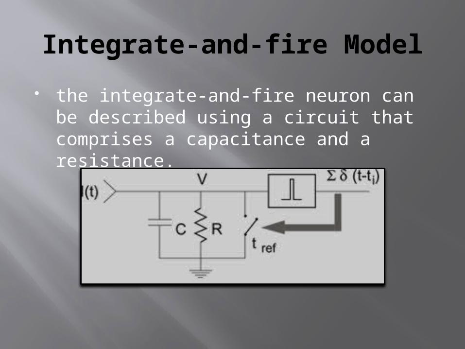
the integrate-and-fire neuron can be described using a circuit that comprises a capacitance and a resistance.

Integrate-and-fire Model

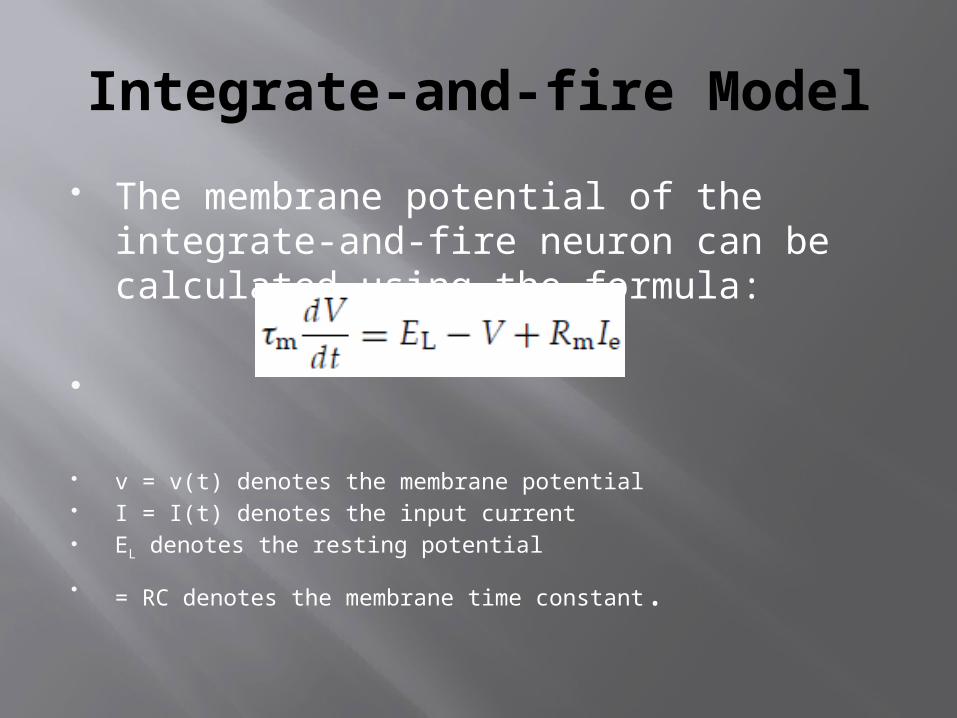
The membrane potential of the integrate-and-fire neuron can be calculated using the formula:

v = v(t) denotes the membrane potential I = I(t) denotes the input current EL denotes the resting potential

= RC denotes the membrane time constant.

Integrate-and-Fire Neuron

The membrane potential in response to a constant injected

current is given by the following equation

v = v(t) denotes the membrane potential I = I(t) denotes the input current R denotes the membrane resistance, C denotes the capacitance, v0 denotes the potential at time t=0,

EL denotes the resting potential = RC denotes the membrane time constant.

Simulation-Software

A simulation-application was developed to demonstrate the behavior of the neuron.

Qt from NOKIA was used in the development.

Software-Snapshots

Neuron Parameters

I/OPlayback functionsTransformations

Image/Video

Simulation

The pre-synaptic activity was ignored, i.e., the spikes delivered by the predecessor neurons were discarded, so the injected current is the only external driving-force of the neuron.

Only one simulation incorporated the pre-synaptic activity, and it was expressed in the form of spike-times included in the injected current’s equation.

Constant Current

The injected current is time-independent and the neuron will fire at fixed time intervals, if its action potentials exceeds the threshold.

The spikes of the neuron in response to a constant current I =0.1 mA. no pre-synaptic activity. C= 2.0 R= 12.0 vreset= -0.5 v0= 0 vth= 1.0. Simulation-Period = 100 seconds.

Alternating Current

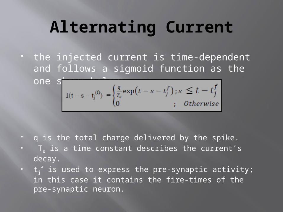
the injected current is time-dependent and follows a sigmoid function as the one shown below:

q is the total charge delivered by the spike. Ts is a time constant describes the current’s decay.

tjf is used to express the pre-synaptic activity; in this case it contains the

fire-times of the pre-synaptic neuron.

Alternating Current

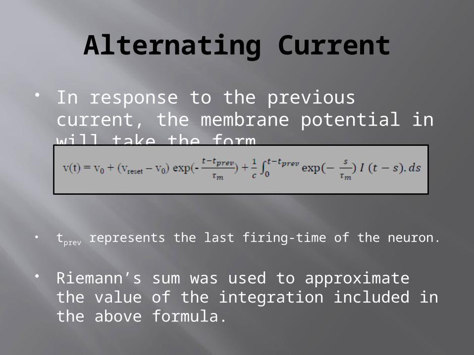
In response to the previous current, the membrane potential in will take the form

tprev represents the last firing-time of the neuron.

Riemann’s sum was used to approximate the value of the integration included in the above formula.

Alternating Current

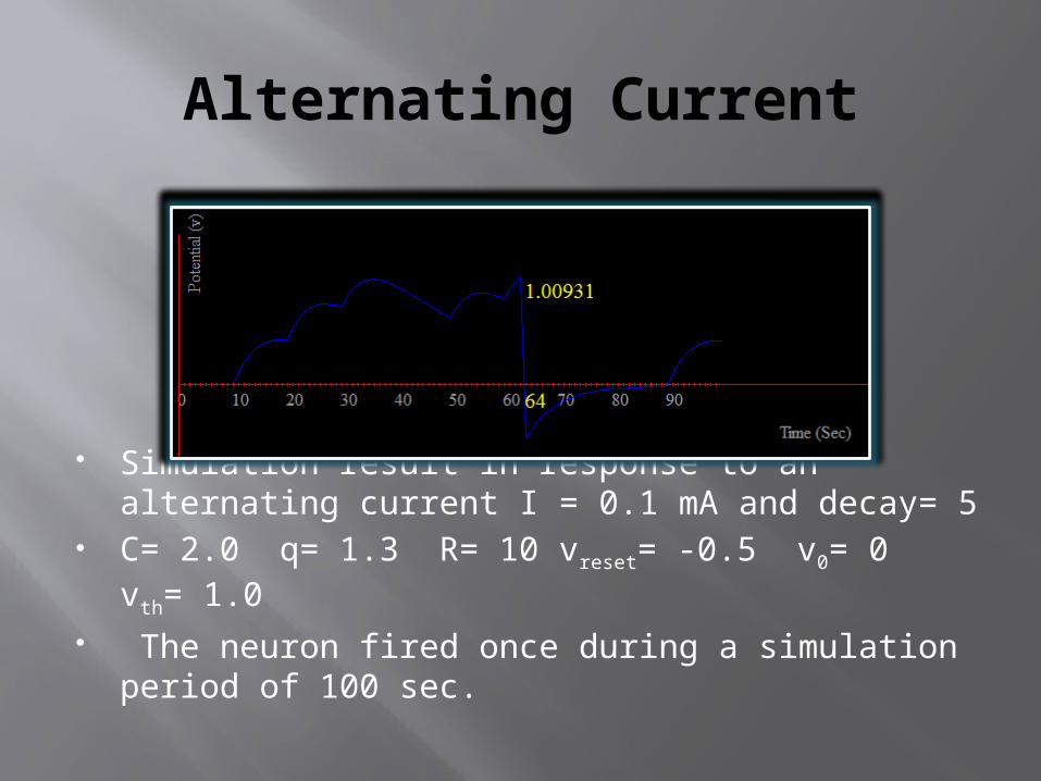
Simulation result in response to an alternating current I = 0.1 mA and decay= 5

C= 2.0 q= 1.3 R= 10 vreset= -0.5 v0= 0 vth= 1.0 The neuron fired once during a simulation period of 100

sec.

Alternating Current

Simulation result in response to an alternating current I = 0.1 mA and decay= 5

C= 2.0 q= 2.0 R= 10 vreset= -0.5 v0= 0 vth= 1.0 The neuron fired twice during a simulation period of 100

sec.

Image-Video Input

The input current in this case will be the intensity value of a pixel in a constant image or a captured video-frame.

The intensity of an RGB pixel is the average of its color components I = (R+G+B)/3

The application provides a grid of 64 neurons arranged in eight rows.

When loading an image or capturing a video-frame, 64 pixels will be taken to form the input currents of the 64 neurons in the grid.

Each neuron is assigned with one pixel and it operates completely independent from all other neurons.

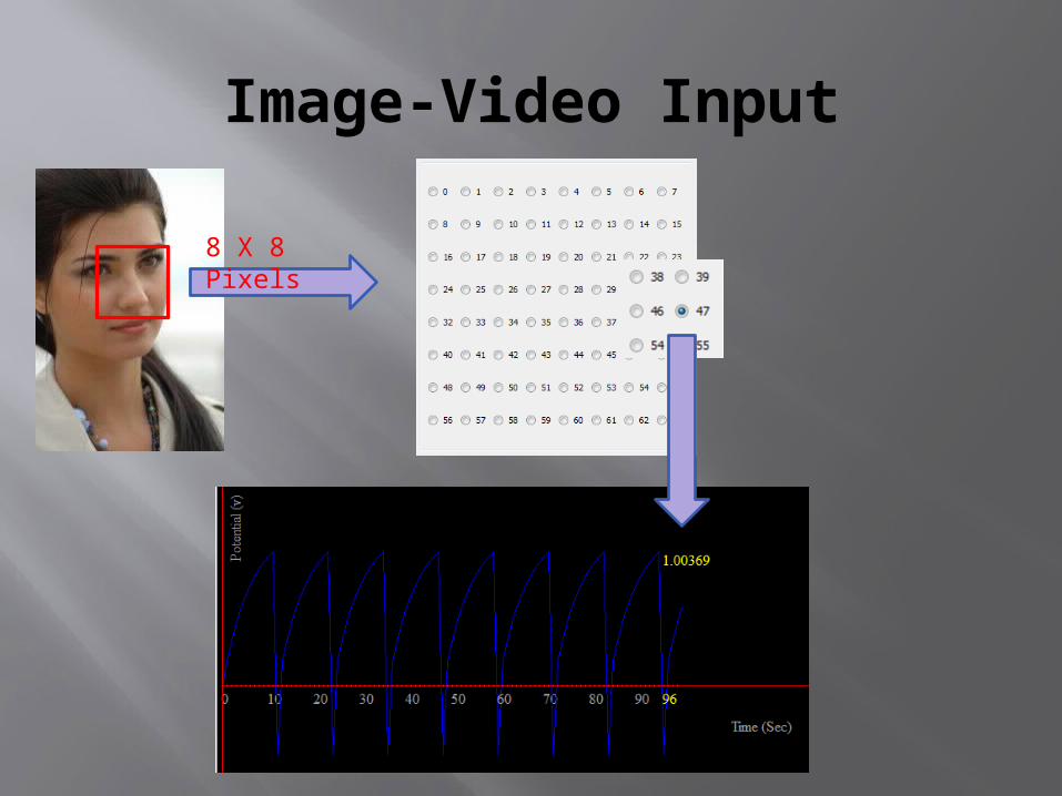
Image-Video Input

8 X 8 Pixels

Transformations - Grayscale

The grayscale value of an RGB pixel is computed using the formula:

grayscale = 0.299 * R + 0.587 * G + 0.114 * B ; R=Red, G= Green, B= Blue

A grayscale transformation reduces the intensity value of the pixel, i.e. , the value of the input current will also be reduced, and a new threshold will be calculated based on the above formula.

Transformations - Grayscale

The spikes the 47th neuron fired in response to the grayscale value of the pixel, the same pixel considered above.

Transformations – Pixel Inverting

Inverting an RGB pixel means to subtract each one of its color components from 255, and then construct a new color from the resulted values.

InvColor= RGB(255 – R, 255 - G, 255 - B); R,G,B represent the color components of the original pixel.

In this case, the neurons that fired when fed with the original pixel, will not fire in response to the pixel-invert and vice versa.

Mappings

Since the value of each color component in a pixel exists in the range of 0..255, so will be the intensity value.

The value of the injected current should also exist in a reasonable range.

For the simulation done here, the range 0..0.5 was chosen to represent the current values.

A mapping is required to map each intensity value to a corresponding value in the range of 0..0.5

CurrValue = (IValue )*0.5 / 255 Vth= (IAVG * 0.5/255 )* Resistance

Video-Frames

Since the first Cathode-Ray-Tube monitor was invented, televisions have been running at 30 frames per second.

This means that the maximum interval for capturing the video frames is ≈ 33.3 ms

In our simulation , a value of 25 ms was chosen. The spike times along with the neurons that fired at these

times were saved in a text file. Each neuron was described using its order in the grid. The contents of the spikes-file were organized in two

columns; the right one contains one spike-time whereas the left contains a number of one neuron that fired at that time.

Video-Frames

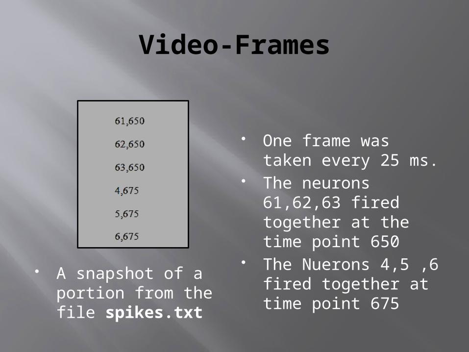
A snapshot of a portion from the file spikes.txt

One frame was taken every 25 ms.

The neurons 61,62,63 fired together at the time point 650

The Nuerons 4,5 ,6 fired together at time point 675

Summary

The integrate-and-fire-neuron is high-sensitive to the changes in the intensity of pixels if its parameters are properly set.

In many applications, such as “Saliency Maps”, that highly depend on the intensity values of a set of pixels, a neural network made of this neuron will perfectly fit.