simulating wave reflection using radiation boundary

Journal of Coastal Research 24 1A 40–48 West Palm Beach, Florida January 2008

Simulating Wave Reflection Using Radiation BoundaryMark J. Clyne and Thomas P. Mullarkey

Civil Engineering DepartmentNational University of IrelandGalway, [email protected]

ABSTRACT

CLYNE, M.J. and MULLARKEY, T.P., 2008. Simulating wave reflection using radiation boundary. Journal of CoastalResearch, 24(1A), 40–48. West Palm Beach (Florida), ISSN 0749-0208.

A finite element wave propagation model for linear periodic waves in a coastal sea region is developed. The modelincludes refraction, diffraction, and reflection of gravity waves on water over arbitrary bathymetry. The authorsdiscuss the use of the computer model in simulating waves using a number of classical examples involving a circularpile, submerged shoal, and breakwater. The method of solution involves complex potential theory. The equation usedby BERKHOFF (1976; Mathematical Models for Simple Harmonic Linear Water Waves—Wave Diffraction and Refrac-tion. Delft: Delft Hydraulics Laboratory, Delft University of Technology, p. 111) and the authors within the domainis elliptic in type allowing wave trains to cross, thereby producing amphidromic points. An amphidromic point is thetwo-dimensional version of a node in a one-dimensional standing wave caused by imperfect reflection or wave traininterference. Radiating and partially reflecting boundaries are modelled by the authors, using a parabolic equationdeveloped in different ways by RADDER (1979; On the parabolic equation method for water-wave propagation, Journalof Fluid Mechanics, 95, 159–176) and BOOIJ (1981; Gravity waves on water with non-uniform depth and current. Delft:Delft Hydraulics Laboratory, Delft University of Technology, p. 127), allowing the passage of energy through a bound-ary over arbitrary bathymetry. RADDER (1979) and BOOIJ (1981) develop this equation in the domain as an alternativeto the elliptic equation. BERKHOFF (1976) uses a downstream radiation boundary condition based on Hankel functionsfor the shoal problem, valid only in constant depth. The upstream boundary condition of BERKHOFF (1976) for thesame shoal problem is derived using the wave ray method. The limitation of the wave ray method is that for generalpurposes the rays frequently cross, resulting in no solution. The method used by the authors has the advantage ofsimplicity in that the boundary conditions are very simple to implement but none of the physical features are lost.

ADDITIONAL INDEX WORDS: Finite element, wave model, refraction, diffraction, reflection, amphidromic points.

INTRODUCTION

In this paper the authors develop a wave propagation mod-el capable of simulating refraction, diffraction, and total re-flection using complex potential theory with an elliptic equa-tion in the domain and a parabolic equation for the absorbingand radiating boundary conditions. Propagation of waterwaves is a phenomenon of great importance to coastal engi-neering practice. It is very difficult to develop a numericalmodel that describes all the physical processes involved inwave propagation; therefore, some simplifications must bemade and only predominant processes are modelled. Fullythree-dimensional solutions would be too complex to developand are not practical to solve, since they are computationallyexpensive; hence, the dimension of the problem is reduced totwo. BERKHOFF (1976) develops an elliptic-type mathemati-cal equation, known as the mild-slope equation, to simulatediffraction, refraction, combined diffraction–refraction, andreflection of water waves around obstacles and over varyingbathymetry. BOOIJ (1981) develops additional terms in orderto include the effects of currents in the elliptic form of themild-slope equation and then simplifies the model into a par-

DOI:10.2112/04-0381.1 received 6 January 2005; accepted in revision2 December 2005.

abolic form, useful when modelling large domains because ofits computational efficiency.

In this paper the authors develop an elliptic wave equationbased on the mild-slope equation for use as the domain equa-tion. Given the elliptic nature of the domain equation, energyis capable of travelling in all directions within the domain;therefore, an absorbing boundary condition is required. Theauthors develop such a boundary condition from the parabolicequations of RADDER (1979) and BOOIJ (1981). For certainmodel configurations wave reflections and backscattering ofwave energy may occur; in this instance open boundaries re-quire a radiation boundary condition. BERKHOFF (1976), aswell as ISAACSON and QU (1989), uses Hankel functions toproduce a radiation condition; however, Hankel functions areonly valid in constant depth. THOMPSON, CHEN. and HADLEY

(1996) and OLIVEIRA and ANASTASIOU (1998) develop a sim-ple form of the radiation boundary condition that doesn’t in-volve Hankel functions. XU et al. (1996) develops a parabolicradiation condition in polar coordinates with an elliptic do-main equation, whereas the authors develop a radiationboundary condition from the parabolic equation of BOOIJ

(1981) in Cartesian coordinates that is valid in arbitrarydepth and can also include such physical features as energydissipation and nonuniform currents. Comparisons are madebetween the results of the authors and those of BERKHOFF

41Simulating Wave Reflection Using Radiation Boundary

Journal of Coastal Research, Vol. 24, No. 1A (Supplement), 2008

Figure 1. Layout of reflecting pile numerical model.Figure 3. The solution of Berkhoff (1976) for normalised wave height(0.1 unit intervals).

Figure 2. Authors’ solution for normalised wave height (0.1 unit inter-vals). Figure 4. Authors’ solution for wave phase (�/4 radian intervals).

42 Clyne and Mullarkey


Figure 5. The solution of Berkhoff (1976) for wave phase (�/4 radianintervals).

Figure 7. Parabolic profile of circular shoal.

Figure 6. Layout of circular shoal numerical model. Figure 8. Authors’ solution for wave phase (�/4 radian intervals).

(1976) for three classical problems. Harbour resonance is in-vestigated using the analytical solution of MEI (1994), whichis also solved numerically by BELLOTTI, BELTRAMI, and GI-ROLAMO (2003); finally, concluding remarks are made.

FUNDAMENTAL EQUATIONS

The mild-slope equation developed by BERKHOFF (1976) isapplied here:

�(a��) � �2a� � 0 (1)

where a � ccg is the product of celerity and group velocity, �is the local wave number, � � (�/�x)i � (�/�y)j is a two-di-mensional differential operator, and � is the two-dimensionalcomplex velocity potential independent of time. Equation 1 isthe result of the vertical integration of an original equationgoverning , the three-dimensional potential including time,where a hyperbolic function is used to represent the verticaldimension. A periodic function is also included to eliminatethe dependence of the potential on time t as shown in Equa-tion 2:

cosh �(z � d) ˜(x, z, t) � �, (2)cosh �d

where � Re{ z is the vertical dimension mea-i� t0�̃ e }�(x),sured upward from the still water level, d is the local waterdepth, t is time, x is the two-dimensional space of x and y,and �0 is frequency observed from a fixed point. Calculationof the wave number is carried out at every node in the do-main by finding the root of the dispersion equation shown inEquation 3.

� g� tanh(�d)2�0 (3)

where g is the acceleration due to gravity.The absorbing boundary condition, using the parabolic

equation of BOOIJ (1981) in the absence of current, is substi-tuted into the boundary integrals of the domain equation con-taining ��1/�n and ��2/�n. The parabolic equation of BOOIJ

(1981) contains two constants P1 and P2. The constants are



Figure 9. The solution of Berkhoff (1976) for wave phase (�/4 radian intervals).

related as follows: P2 � P1 � 0.5, resulting from a binomialexpansion of wave number terms. P1 and P2 do not approxi-mate Equation 1 if the difference between P1 and P2 is some-thing other than 0.5, which was confirmed to the authors byBOOIJ (personal communication). The authors use P1 � 0.0and P2 � 0.5, reducing the equation to the same one as thatof RADDER (1979). RADDER (1979) uses a matrix splittingmethod to produce his parabolic equation, whereas BOOIJ

(1981) uses the pseudo-operator method. The parabolic equa-tion of RADDER (1979) and BOOIJ (1981) is as follows (termscontaining P1 are omitted since P1 � 0.0),

�� 1 �(a�) iP � �2� i� � a � � f (�) (4)� �[ ]�n 2a� �n a� �s �s

where s is tangential to the boundary and perpendicular ton the outward normal and i is the imaginary operator wherei � �1. An extension of the absorbing boundary conditionis the radiation boundary condition, which uses the parabolicabsorbing equation to allow backscattered wave energy topass through a boundary while containing the incident waveinformation. In order to develop the radiation condition, thefull potential must be separated into its incident and scat-tered components shown in Equation 5, the scattered poten-tial obeying Equation 4.

I S S I� � � � � � � � �

S�� S I I� f (� ) (� � ) � f (� � )

�n �n

I�� I� f (�) f (� ) �

�n �n(5)

where f(�) is the right-hand side of Equation 4, �S is theunknown scattered potential, and �I is the known incidentpotential developed from one-dimensional solutions along therequired boundaries. After the solution is completed the com-plex potential � � �1 � i�2 is converted into the complexwater surface elevation:

�0� � i �, (6)g

where � � �1 � i�2.The complex water surface elevation � in Equation 6 is

combined with a periodic function to produce the real watersurface for an arbitrary value of time t, as seen in Equation 7.

i� t0�̃(x, t) � Re{e �(x)} � � cos � t � � sin � t. (7)1 0 2 0

RESULTS

The authors will verify their solutions below using three ofthe classical problems of BERKHOFF (1976): the circular re-flecting pile, the semi-infinite breakwater, and the circularshoal. And the authors verify their simulation of harbour res-onance by means of the analytical solution of MEI (1994).

Reflecting Pile

To simulate wave propagation around a perfectly reflectingcylinder of a circular cross section, a finite element model isgenerated using triangular elements as per the configurationin Figure 1. A wave of period 1.1868 seconds propagates fromthe top to the bottom of the domain over a constant waterdepth of 4.0 m, with an upstream boundary wave height of0.1 m.



Figure 10. Authors’ solution for normalised wave height (0.25 unit intervals).

Following the authors’ numerical solution, a plot for nor-malised wave height, i.e., height divided by incident height,is produced as seen in Figure 2, which illustrates the varia-tion in wave height due to reflection and diffraction of waveenergy.

Boundaries have been placed away from the area of inter-est to prevent them from adversely affecting the solution.Large wave heights occur upstream of the pile, where an an-tinode occurs at the perfectly reflecting boundary of the pile.Wave energy travels around the pile due to diffraction, thesheltering effect of the pile leads to low wave height on thedownstream boundary of the pile. The authors’ numerical so-lution in Figure 2 compares well with the analytical solutionof BERKHOFF (1976) shown in Figure 3.

Figure 4 shows the pattern of wave crests, or phase lines,formed when waves propagate around a reflecting pile.Downstream of the pile a diffraction pattern is observedwhere the phase lines maintain an angle of 90 with the sur-face of the pile. Upstream of the pile the reflection field caus-es wavelengths to change because of the interaction of inci-dent waves with scattered ones.

Very good agreement can be seen between the authors’ nu-merical solution in Figure 4 and the analytical solution ofBERKHOFF (1976) in Figure 5.

Circular Shoal

To demonstrate the behaviour of gravity waves propagat-ing over a circular shoal, the numerical model shown in Fig-ure 6 is developed. Boundaries have been placed away fromthe area of interest to prevent them from adversely affectingthe solution.

Wave refraction, diffraction, and backscattering occur fromthe raised portion of the seabed whose parabolic profile isillustrated in Figure 7.

Phase lines form the pattern in Figure 8 over the shoal.Upstream of the shoal the phase lines are distinct and varyslowly as they refract over the reducing depths, in contrastto the complicated pattern of wave diffraction and interac-tions occurring downstream of the crest of the shoal, whichcauses the occurrence of amphidromic points where wavetrains overlap.

Very good agreement is observed between the plots of theauthors’ numerical solution in Figure 8 and that of BER-KHOFF (1976) in Figure 9. The location and number of am-phidromic points or nodes compare very well also.

Wave energy focusing occurs just downstream of the crestof the shoal, with a magnitude of three times that of the in-cident wave energy illustrated by the maximum in Figure 10.It can be seen from comparison of Figure 8 with Figure 10that at amphidromic points the wave height approaches zero.

Figure 11 shows that the solution of BERKHOFF (1976) fornormalised wave height produces a larger maximum thanthat of the authors in Figure 10. This is due to differences inthe boundary conditions used. BERKHOFF (1976) uses a con-strained upstream boundary with incident wave data takenfrom a ray solution, while the authors use a radiation bound-ary condition upstream and on the two sides to allow thebackscattering of wave energy out of the domain.

Semi-Infinite Breakwater

To investigate the behaviour of waves that propagate to-ward a reflecting semi-infinite breakwater, the numerical



Figure 11. The solution of Berkhoff (1976) for normalised wave height (0.25 unit intervals).

Figure 12. Layout of semi-infinite breakwater numerical model.

model in Figure 12 is used. Waves propagate in a directionnormal to the breakwater and reflect from it, causing stand-ing waves to occur while wave energy also diffracts aroundthe tip of the breakwater and downstream of the breakwater.Boundaries have been placed away from the area of interestto prevent them from adversely affecting the solution. Wavesincident on a reflecting breakwater exhibit the phase patternshown in Figure 13, whereby the interaction of incident andreflected waves produces nodes or amphidromic points illus-trated by the points of intersection of wave phase in Figure13.

As waves diffract around the breakwater they maintain anangle of 90 with the downstream face of the breakwater. Thecomplicated phase line pattern upstream of the breakwateris illustrated by the use of a small contour interval of 2.5 compared with the 20 intervals elsewhere.

The authors’ numerical solution in Figure 13 is similar tothe analytical solution of BERKHOFF (1976) in Figure 14. Theauthors’ plot of normalised wave height in Figure 15 showsthat there is a significant sheltering effect downstream of thebreakwater as the wave height reduces to less than 25% ofthe incident value. Upstream of the breakwater wave heightsvary rapidly from maximums to minimums. Positions wherewave heights approach zero coincide with locations of phase



Figure 13. Authors’ solution for wave phase (2.5 and 20 degree inter-vals).

Figure 14. The solution of Berkhoff (1976) for wave phase (2.5 and 20degree intervals).

Figure 15. Authors’ solution for normalised wave height (0.1 and 0.05unit intervals).

line intersections known as amphidromic points, this is evi-dent when comparing Figure 13 with Figure 15.

The analytical solution of BERKHOFF (1976) in Figure 16is similar to the authors’ numerical solution in Figure 15.

Harbour Resonance

A narrow bay of finite length shown in Figure 17 illustratesmany common features of harbour resonance. The nodal den-sity of the mesh in Figure 17 is such that for the smallestperiod there are approximately 30 nodes per wavelength. Inorder to model the waves for this type of harbour configura-tion the solution is separated into two parts. First an analyt-ical solution of the standing wave against the straight coast-line is calculated. Second waves are simulated with the har-bour present, which causes scattered waves to propagate outfrom the harbour mouth. Open boundaries are subject to theradiation boundary condition, which contains incident wavedata in the form of the analytical standing wave calculatedprior to solution.

Separating the solution into two parts allows the two setsof scattered waves, namely, the reflected waves from an in-finitely long cliff and the scattered waves from the harbour,to be modelled independently. Modelling the problem as oneset of scattered waves causes the reflected wave from thestraight boundary to be distorted as a result of the superpo-sition of this wave with the scattered wave from the mouthof the harbour. The analytical solution of MEI (1994), Equa-



Figure 16. The solution of Berkhoff (1976) for normalised wave height(0.1 and 0.05 unit intervals).

Figure 17. Layout of harbour resonance numerical model.

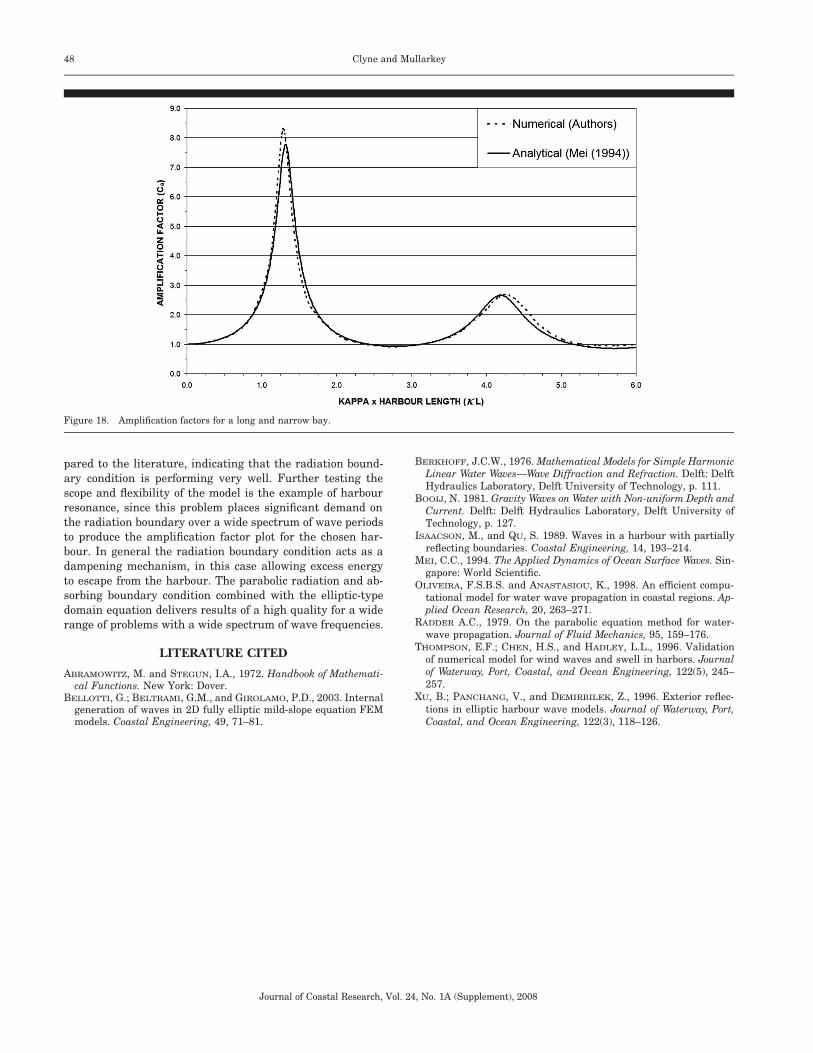
tion 8 for the amplification factor due to harbour resonancein this type of bay, is illustrated in Figure 18.

1C � (8)a cos �L � (2�a/�)sin �L ln(2��a/�e) i�a sin �L

where L is the length of the harbour, a is half the width ofthe harbour, e is the base of the natural logarithm (e �2.71828. . .), and � is Euler’s constant; however, in this in-stance MEI (1994) redefines Euler’s constant to be ln � �0.5772157, for tidier notation. As part of the derivation ofEquation 8 by MEI (1994), an inner approximation using theABRAMOWITZ and STEGUN (1972) expansion of the far-fieldsolution for a standing and radiating wave in the vicinity ofthe harbour entrance reduces the term containing a H Han-(1)

0

kel function in the far-field solution to two terms in the ap-proximation, one of which contains �. The ABRAMOWITZ andSTEGUN (1972) expansion is based on an ascending series forsmall values of the general complex independent variable; inthis case MEI (1994) uses the real form of the independentvariable. The authors calculate the numerical amplificationfactor using Equation 9, where Hincident is the incident waveheight and Hrecorded is the recorded height at the end of thechannel at the centre of the back wall.

1 HrecordedC � . (9)a 2 Hincident

Derivation of the analytical solution of MEI (1994) consistsof this technique of separating the scattered wave into its twocomponents, the reflected wave from the straight coastlineplus the scattered wave from the harbour. Good agreementis found when comparing the authors’ numerical solution

with the analytical solution of MEI (1994) in Figure 18. InFigure 18 the harbour length is 0.3 m. Some relevant valuesextracted from Figure 18 are as follows: at the larger peakthe wavelength is just less than five times the harbourlength, and at the smaller peak it is just less than 1.5 timesthe harbour length. Numerical simulation generates an am-plification factor of somewhat greater magnitude than theanalytical solution at the larger peak; this may be due in partto the size of the domain, since at the larger peak the lengthof the wave is much greater than the harbour length for thisresonance event. The amplification factor at the second peakis in better agreement.

CONCLUSIONS

The examples in the results section are chosen to test theperformance of the radiation boundary condition by subject-ing it to various forms of radiated and scattered wave energyfrom different shaped reflecting obstacles, boundaries, andseabed features. In all the examples presented the resultshave been very favourable for the authors’ model when com-



Figure 18. Amplification factors for a long and narrow bay.

pared to the literature, indicating that the radiation bound-ary condition is performing very well. Further testing thescope and flexibility of the model is the example of harbourresonance, since this problem places significant demand onthe radiation boundary over a wide spectrum of wave periodsto produce the amplification factor plot for the chosen har-bour. In general the radiation boundary condition acts as adampening mechanism, in this case allowing excess energyto escape from the harbour. The parabolic radiation and ab-sorbing boundary condition combined with the elliptic-typedomain equation delivers results of a high quality for a widerange of problems with a wide spectrum of wave frequencies.

LITERATURE CITED

ABRAMOWITZ, M. and STEGUN, I.A., 1972. Handbook of Mathemati-cal Functions. New York: Dover.

BELLOTTI, G.; BELTRAMI, G.M., and GIROLAMO, P.D., 2003. Internalgeneration of waves in 2D fully elliptic mild-slope equation FEMmodels. Coastal Engineering, 49, 71–81.

BERKHOFF, J.C.W., 1976. Mathematical Models for Simple HarmonicLinear Water Waves—Wave Diffraction and Refraction. Delft: DelftHydraulics Laboratory, Delft University of Technology, p. 111.

BOOIJ, N. 1981. Gravity Waves on Water with Non-uniform Depth andCurrent. Delft: Delft Hydraulics Laboratory, Delft University ofTechnology, p. 127.

ISAACSON, M., and QU, S. 1989. Waves in a harbour with partiallyreflecting boundaries. Coastal Engineering, 14, 193–214.

MEI, C.C., 1994. The Applied Dynamics of Ocean Surface Waves. Sin-gapore: World Scientific.

OLIVEIRA, F.S.B.S. and ANASTASIOU, K., 1998. An efficient compu-tational model for water wave propagation in coastal regions. Ap-plied Ocean Research, 20, 263–271.

RADDER A.C., 1979. On the parabolic equation method for water-wave propagation. Journal of Fluid Mechanics, 95, 159–176.

THOMPSON, E.F.; CHEN, H.S., and HADLEY, L.L., 1996. Validationof numerical model for wind waves and swell in harbors. Journalof Waterway, Port, Coastal, and Ocean Engineering, 122(5), 245–257.

XU, B.; PANCHANG, V., and DEMIRBILEK, Z., 1996. Exterior reflec-tions in elliptic harbour wave models. Journal of Waterway, Port,Coastal, and Ocean Engineering, 122(3), 118–126.

simulating wave reflection using radiation boundary

Documents