Simulation and Health Economics

Introduction Recent research publications are recognizing that economic modeling which does not take into account waiting times and delays and their impact on the effect of treatment and costs can be erroneous. Discrete event simulation is being increasingly recommended as an economic evaluation technique.

Economic evaluations take place when a new drug or device is being taken to market and is also used by healthcare payers and providers when considering whether to adopt any innovation.

Clinicians and administrators need to understand not just whether the new intervention is cost effective when applied to theoretical cohorts of patients, but also what it would mean when implemented in their own organization or health economy.

Will it require increased staff capacity, or will it free up time?

Will it reduce patient waiting times for a service?

How will it impact on the patients seen in our clinic or hospital?

Using discrete event simulation allows modelers to simulate both the transition between disease states and their likely costs and QALYs as well as to understand how the individual patient will now use services and resources. Decision-makers will need to be assured on all these points prior to approving a business case for implementation of a new way of working or the adoption of a drug or device.

Ron Shannon from GHE lists the following reasons to use discrete event simulation, it:

represents clinical reality

presents the course of disease naturally with few restrictions

is flexible: no mutually exclusive branches or states required

follows the natural concept of time, the simulation clock keeps track of the passage of time (no fixed cycles)

offers flexibility for handling perspectives and sensitivity analyses

permits transparency

allows queuing (e.g., if a health resource is not available at a given time)

enables modeling of limited resources, bottlenecks, if applicable to the problem

defines patients as explicit elements with specific attributes (e.g., sex, age, event history) that can be

modified over time

provides the option of updating variables continuously or at specific time periods

and, in economic evaluations, discrete event simulation has the flexibility to accommodate a richer structure

without making it unmanageable in size

While many health economists are using discrete event simulation, others prefer Monte Carlo and Markov

models. SIMUL8 Professional combines state transition modeling with discrete event simulation to allow users to

have the full flexibility to model key healthcare questions.

Getting Started Guide We have developed this guide to enable health economists and decision-makers new to SIMUL8 to

learn how to use the software for this purpose. It takes you through the key features via a case study

and explains how to use them to get you up and running quickly.

The guide will cover the following material:

What are State Charts

Building a disease model

Defining Transitions

Sub States

Creating custom results

Recording Utility Values

Calculating QALY’s

Combining a Disease Model with a Discrete Process

Costs

Graphics

SIMUL8 Case Study - Disease Model The most important part of your simulation will be modeling the disease/condition as the different

stages of the disease will determine what treatments, costs or resource are required by the

patient. The simplest way to do this in SIMUL8 is to use State Charts.

State Charts

State charts allow you describe what is happening to the patient in a supplemental way to a

typical discrete process. This significant benefit of using the method is that it removes the need

for complicated logic. They describe a series of states (conditions) through which patients will

flow. Typically the flow through a series of states is not related to the physical position of the

patient. Instead we can link the physical position of the patient by triggering events in a discrete

process which depend on which state (condition) the patient is in.

State charts are made up of States, Decisions and Transitions;

- States are used to describe the various condition which the disease can progress

through. These could be Low, Moderate or Severe stages of a disease.

- Decisions are used when a patient transitions from the state but a decision as to what

state they will transition too happens. Such as from the state Low 50% of patients will

transition to Moderate and 50% to High.

- Transition arrows allow you to control how a patient transitions from one state to

another. There are various options to how patient can transition such as chance per day or a

distribution of time spent in state.

Building the Disease Model

To build your disease model simply

drag and drop states and/or decision

points from the building blocks tab at

the left hand side. Once all the required

states are on screen these can be

connected up with transition arrows. To

connect states with transition arrows

hold down the Shift key and click and

drag from state to state to create an

arrow. Transition arrows can go both to

and from states.

For this guide we will be using an

example model to talk through the

concepts, the example model is based

on a project looking at the cost

effectiveness of different treatments for

Chronic Venus Leg Ulcers. The disease

pathway is outlined in Figure 1. Figure 1 : Leg Ulcer Disease Pathway

State Properties Once you have dropped your required states on screen we can then populate these with

properties. State properties are accessed in the same way as any other SIMUL8 object, by

selecting the object and using the ribbon menus or by

double clicking on the object.

Under the state preferences tab, the first box is where

you can name the state. By doing so SIMUL8 will

automatically create a label also with this name as States

require labels to work. Alternatively you can select a pre

defined label and SIMUL8 will automatically set the name

of this state to the label.

Also within this tab we can define start up values for the states, in the example model in Figure 1

this is used to define the patient cohort that will be run through the model. All patients will start in

the state Uncomplicated Ulcer, to do this enter a value in the box named ‘Initial Content’.

State Transitions The next step is to define how patients will transition from state to state, to enter these properties

double click on a transition arrow.

Select a transition type from the drop down menu, a short description of each transition type is

provided below;

Transition Type Description

Chance each per time unit Enter the chance each patient has of transitioning

per time unit.

Percent of all per time unit Enter the percentage of patients that will transition

per time unit.

Elapsed time in state Enter the time it will take for a patient to transition.

Rate (number per time unit) Enter the number of patients that will transition per

time unit.

Time of day

One every N time units Enter the time at which one patient will transition.

All every N time units Enter a time unit in which all patients will transition.

Always Patients entering this state will always transition.

When selecting a transition type it is important to remember that the transitions are based on the

simulation time units. By default SIMUL8 sets the simulation time units to minutes, to change these

settings go to the Data and Rules Tab and select clock properties and select from the required unit

from the top. For the ulcer example model select the setting “Days”.

In the ulcer example model there are three transition types used, the first is Chance each per time unit. The table

below outlines the values and states that use these transitions.

The transitions Clinical Infection and Skin Disorder back to Uncomplicated and Severe Infection to Very Ill are based

on a distribution, meaning that patients are likely to spend a certain amount of time in that state before transitioning.

To create distributions select the data and rules tab and distributions, use the data below to create the distributions

required for the ulcer example.

From State To State Chance per day

Uncomplicated Death 0.000131

Uncomplicated Clinical Infection 0.000548

Uncomplicated Skin Disorder 0.0000224

Clinical Infection Severe Infection 0.0000167

Severe Infection Death 0.000141

Distribu on Name Time in State (days)

Clinical Infec on 9

Severe Infec on 9

Skin Disorder 8

Distribu on Type

Average

Average

Average

Once the distributions have been created apply them to correct transition arrow. To so this first

select the transition type Elapsed time in state, use the (…) to open the formula editor and select the

correct distribution. Distributions can be found by selection the ‘Object’ option at the left hand side. The

table below shows which distributions should be applied to each transition.

The final transition is that from Uncomplicated to Healed Wound, this is based on a percentage chance of

healing which changes each week the patient is receiving treatment. To set up this transition the heal time data

needs to be entered into an internal spreadsheet. To do this select the data and rules tab then the information

store and create a new spreadsheet, next copy and paste the heal time data into it. The heal time data can be

found at the end of this guide.

The next step is to set the Healed Wound transition, double click the arrow and select the transition type

percent of all per time unit. Like with the distributions use the (…) button to reference the spreadsheet. All

spreadsheets are found in ‘Information’

After selecting the spreadsheet the column and row from which to read the data needs to specified. The column

will always be 2 and the row will be based on the week. There is a MATH function WEEK to control this which

will automatically increment the row depending on what week the simulation is running by using the reserved

SIMUL8 variable ‘Simulation Time’. The images below outline how this should be populated.

From State To State Distribution Name

Clinical Infection Uncomplicated Clinical Infection (9,Average)

Skin Disorder Uncomplicated Skin Disorder (8, Average)

Severe Infection Very Ill Severe Infection (9, Average)

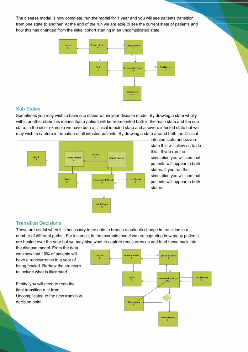
The disease model is now complete, run the model for 1 year and you will see patients transition

from one state to another. At the end of the run we are able to see the current state of patients and

how this has changed from the initial cohort starting in an uncomplicated state.

Sub States Sometimes you may wish to have sub states within your disease model. By drawing a state wholly

within another state this means that a patient will be represented both in the main state and the sub

state. In the ulcer example we have both a clinical infected state and a severe infected state but we

may wish to capture information of all infected patients. By drawing a state around both the Clinical

infected state and severe

state this will allow us to do

this. If you run the

simulation you will see that

patients will appear in both

states. If you run the

simulation you will see that

patients will appear in both

states.

Transition Decisions These are useful when it is necessary to be able to branch a patients change in transition in a

number of different paths. For instance, in the example model we are capturing how many patients

are healed over the year but we may also want to capture reoccurrences and feed these back into

the disease model. From the data

we know that 10% of patients will

have a reoccurrence in a year of

being healed. Redraw the structure

to include what is illustrated.

Firstly, you will need to redo the

final transition rule from

Uncomplicated to the new transition

decision point.

By double clicking on the transition decision you can select from 3 routing options. Select percentage

and enter 90% to Healed Wound and 10% to Reoccurrence. Lastly define the transition between

Reoccurrence and uncomplicated wound, as this can happen at any point in the year select the “Elapsed

Time” option and use a uniform distribution between 1 and 365 days.

State Actions/Events State events are a useful feature in being able to produce your own custom results or attaching information to

individual patients. State actions/events can be accessed on the ribbon or by double clicking a state. For the

ulcer example the total number of Severe Infections, Clinical Infections and Skin Disorders over the year

needs to be displayed.

For this global number variables for each result need to be created , these are created in the information store,

the same way as the spreadsheet was created.

Once these have been created, select the State Action “On Join” and chose the option “Change Anything”.

Now select the appropriate variable using the formula editor, global variables can be found in “Information”.

Next chose the Action “Increment” form the right hand side, this will then automatically increment the variable

by 1 each time a patient enters the particular state.

You can also utilize SIMUL8’s visual data feature so that you can see these results onscreen. To do so, go to

the insert tab and select visual data. Next click the area on the screen where you wish the data to be displayed

and then select from the drop down the appropriate variable.

Now run the simulation and you will be able to see on screen the total amount of patients who have

entered that state.

The same principal can be applied if you are wanting to attach information to individual patients, for instance if

you were wanting to record utility values in order to calculate QALY’s. In SIMUL8, labels are used to do this, to

create a label go to Data and Rules Tab and select Labels. Once you have created a label select a state and

then as with the global variables you can select either “Actions on Join” or “Actions on Leave”, the value of the

label can then be changed to store particular information about that patient. For example in the ulcer example we

can set the utility value for each patient depending on what state they are. In the image below we are setting the

utility label to 0.4 to represent the value associated with being the state “Severe Infection”.

In calculating QALY’s the amount of time spent in that state also needs to be recorded, using another label

called “Time In” the time at which a patient enters this state can be recorded using “Action on Join”.

Then on using “Actions on Leave” we can then calculate the QALY for that individual patient. First

create a label named “QALY”. Select the “Set to” option and chose fixed, you can then use the (…)

button to open the formula editor. This allows you to enter a calculation, the below image shows the

calculation used in this example.

It takes the current simulation time and subtracts the label value that contains the time that the

patient entered the state. This is then multiplied by the utility value and this information is then stored

in the label “QALY”.

Combining the Disease Model with a Discrete Process State charts are useful for modeling the disease pathway and how patients transition from different

states but it is also useful to be able to combine these with traditional discrete process. For instance

in the ulcer example we want to simulate that the patient will have a hospital stay should they

transition into Clinical Infection. To do this first create the process outlined below using the traditional

SIMUL8 building blocks.

Once this is created the next step is to trigger a patient arrival to this process, this can be done by

selecting the Clinical Infection state and choosing the Events tabs. Here you can select from all start

points in your model and this will cause the patient in the state to arrive at the discrete process.

Before running the simulation make sure that the check box

“Remove from all states” is unchecked. This is found by double

clicking the End object in the process.

If this is checked then when patients have gone through the

treatment then they will also be removed from the state charts. This

is a useful feature if an outcome of the process would result in the

patient being removed from the disease model. However in this

example, after treatment the patient will continue to transition in the

disease model

If you run the simulation as is you will get the results shown below,

you will notice that the number of arrivals does not match the total

number of clinical infections recorded in our results. This is because

current we only have the capacity to treat 1 patient at a time in our

discrete process. As you can see from the queue we have a large build up of patients waiting for a

bed, patients are waiting so long for a bed that they have transitioned out of the clinical infection

state. At some point over the year they have transitioned back to an infected state but this time an

arrival will not be triggered as in reality they are still waiting on a bed.

This is one of the key benefits of using simulation as you can now start to explore the effect of

capacity on your outcomes. By selecting the Activity “Treatment for Severe Infection” we can

increase the capacity by using the replicate function found on the activity’s “Additional” tab.

If you increase this to 10 and run the simulation this problem no longer occurs as we have sufficient

capacity to deal with all infections. However in reality it may be that we don't have the capacity to

To do this reduce the replications to 5 and add the additional objects shown below to the process.

Next set the Shelf life of the queue to 3 and the routing in of “Treatment for Severe Infection” to

Expired Only. Set the Treatment for severe Infection to a dummy activity by making the activity timing

a fixed 0 and ensure the end point has the remove from all states unchecked.

The aim of this process is to simulate what happens to patients if they cannot get a bed for treatment

of an infection. By setting a shelf life this means that any patient that has to wait longer than 3 days

will move down a different path. We now want the simulation to escalate the patients condition,

essentially over riding the traditional state transitions, should patients not get a bed within 3 days. As

states are controlled via label values we can do this by using label actions on “Treatment for Severe

Infection”. Set the label Clinical Infection to 0 and the label Severe Infection to 1.

Now run the simulation again and we can see that as a result of lack of capacity we have an

increased amount of Severe Infections. By modeling this it allows you to think about the effects of

capacity on patient outcomes and how this may differ with treatment options.

As well as being able to trigger arrivals and control the state charts, the time spent in activities can

also be linked to the disease model. In the ulcer example patients will require a bed whenever they

have a clinical or severe infection. The disease model controls when they will transition back to an

uncomplicated state so in the discrete process we want to ensure that the patient will remain in a bed

until they transition back to a healthy state.

Select the object Treatment for Infection and on the Ribbon select Addition and then Timing.

Choose the bottom option and select Uncomplicated Wound from the list. This will now ensure

that the patient will stay in the activity until they transition back to an uncomplicated state.

Costs If you have connected your disease model to a discrete process you can use the traditional building blocks to

apply costs to your simulation. On each tradition simulation

object there is a costs option which is accessed by selecting the

object , Properties and Finance. In the ulcer example we can

apply a cost per day that would be incurred due to the patient

being in a hospital bed.

Cost results are displayed in the income statement which is

found on the home tab. This will give you a breakdown of where

all the costs incurred in the model are. Like all results in

SIMUL8 you can add these to the results summary by hovering

over the result and right clicking. This is helpful when

comparing runs.

Costs can also be applied using the method discussed in State

Actions, where you can increment variables or spreadsheets

when a patient enters or exits a state. If you require more

complicated cost functions which require rules then you can

also access Visual Logic. Each state has a number of events

where you can code conditional statements in the visual logic

editor. Select a state and on the properties tab on the ribbon

chose Events, after selecting an event this will then open the Visual Logic editor.

Graphics Making your simulation visibly compelling can really help when telling the simulation story. Each

simulation object and state chart has the ability to easily change the graphics to help you do this. For

state chart graphics you can change the object shape and fill color as well as adding in your own image

to represent the state.

To change a states graphics first select a state and then the graphics tab on the ribbon, the image

below gives an example of what is possible with state chart graphics.

Heal Time Data

Week 1 0

Week 2 0

Week 3 0

Week 4 0

Week 5 0.04

Week 6 0.06

Week 7 0.12

Week 8 0.16

Week 9 0.23

Week 10 0.25

Week 11 0.29

Week 12 0.29

Week 13 0.41

Week 14 0.41

Week 15 0.41

Week 16 0.41

Week 17 0.43

Week 18 0.43

Week 19 0.55

Week 20 0.55

Week 21 0.62

Week 22 0.64

Week 23 0.69

Week 24 0.69

Week 25 0.72

Week 26 0.72

Week 27 0.72

Week 28 0.72

Week 29 0.73

Week 30 0.73

Week 31 0.74

Week 32 0.75

Week 33 0.75

Week 34 0.76

Week 35 0.76

Week 36 0.76

Week 37 0.76

Week 38 0.76

Week 39 0.77

Week 40 0.77

Week 41 0.77

Week 42 0.78

Week 43 0.79

Week 44 0.8

Week 45 0.81

Week 46 0.82

Week 47 0.83

Week 48 0.84

Week 49 0.84

Week 50 0.84

Week 51 0.84

Week 52 0.84

Week 53 0.84